Fundamentals of Multimedia, Chapter 8 Chapter 8 Lossy Compression Algorithms 8.1 Introduction 8.2 Distortion Measures 8.3 The Rate-Distortion Theory 8.4 Quantization 8.5 Transform Coding 8.6 Wavelet-Based Coding 8.7 Wavelet Packets 8.8 Embedded Zerotree of Wavelet Coe cients ffi 8.9 Set Partitioning in Hierarchical Trees (SPIHT) 8.10 Further Exploration 1 Li & Drew c Prentice Hall 2003
Transcript
Fundamentals of Multimedia, Chapter 8
Chapter 8
Lossy Compression Algorithms
8.1 Introduction8.2 Distortion Measures
8.3 The Rate-Distortion Theory
8.4 Quantization
8.5 Transform Coding
8.6 Wavelet-Based Coding
8.7 Wavelet Packets
8.8 Embedded Zerotree of Wavelet Coefficients
8.9 Set Partitioning in Hierarchical Trees (SPIHT)
8.10 Further Exploration
1 Li & Drew c Prentice Hall 2003
Fundamentals of Multimedia, Chapter 8
8.1 Introduction
• Lossless compression algorithms do not deliver compressionratios that are high enough. Hence, most multimedia com-pression algorithms are lossy.
• What is lossy compression ?
– The compressed data is not the same as the original data,but a close approximation of it.
– Yields a much higher compression ratio than that of loss-less compression.
2 Li & Drew c Prentice Hall 2003
SN R = 10 log10 2
Fundamentals of Multimedia, Chapter 8
8.2 Distortion Measures
• The three most commonly used distortion measures in imagecompression are:
– mean square error (MSE) σ 2,
σ 2 =1
N
N
(xn − yn)2
n=1
(8.1)
where xn, yn, and N are the input data sequence, reconstructed datasequence, and length of the data sequence respectively.
– signal to noise ratio (SNR), in decibel units (dB),
σx2
σd(8.2)
where σx2 is the average square value of the original data sequenceand σd2 is the MSE.
– peak signal to noise ratio (PSNR),
P SN R = 10 log10x2peak
σd2(8.3)
3 Li & Drew c Prentice Hall 2003
0
Fundamentals of Multimedia, Chapter 8
8.3 The Rate-Distortion Theory
• Provides a framework for the study of tradeoffs between Rateand Distortion.
R(D)
H
D
D max
Fig. 8.1: Typical Rate Distortion Function.
4 Li & Drew c Prentice Hall 2003
Fundamentals of Multimedia, Chapter 8
8.4 Quantization
• Reduce the number of distinct output values to a muchsmaller set.
• Main source of the “loss” in lossy compression.
• Three different forms of quantization.
– Uniform: midrise and midtread quantizers.
– Nonuniform: companded quantizer.
– Vector Quantization.
5 Li & Drew c Prentice Hall 2003
Fundamentals of Multimedia, Chapter 8
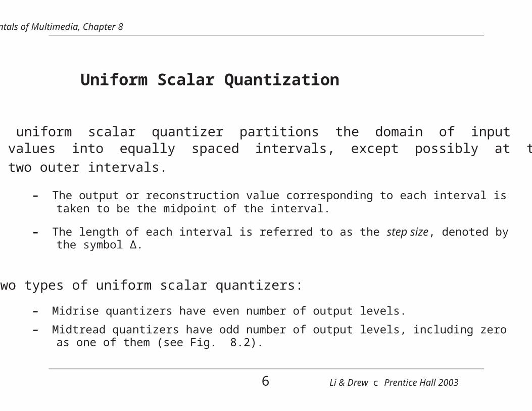
Uniform Scalar Quantization
• A uniform scalar quantizer partitions the domain of inputvalues into equally spaced intervals, except possibly at thetwo outer intervals.
– The output or reconstruction value corresponding to each interval istaken to be the midpoint of the interval.
– The length of each interval is referred to as the step size, denoted bythe symbol ∆.
• Two types of uniform scalar quantizers:
– Midrise quantizers have even number of output levels.
– Midtread quantizers have odd number of output levels, including zeroas one of them (see Fig. 8.2).
6 Li & Drew c Prentice Hall 2003
Fundamentals of Multimedia, Chapter 8
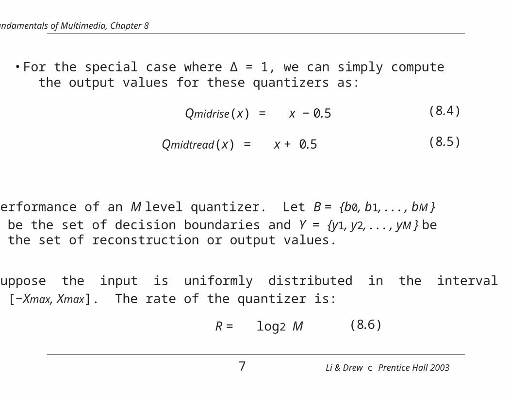
• For the special case where ∆ = 1, we can simply computethe output values for these quantizers as:
Qmidrise(x) = x − 0.5
Qmidtread(x) = x + 0.5
(8.4)
(8.5)
• Performance of an M level quantizer. Let B = {b0, b1, . . . , bM }be the set of decision boundaries and Y = {y1, y2, . . . , yM } bethe set of reconstruction or output values.
• Suppose the input is uniformly distributed in the interval[−Xmax, Xmax]. The rate of the quantizer is:
• Granular distortion: quantization error caused by the quan-tizer for bounded input.
– To get an overall figure for granular distortion, notice that decisionboundaries bi for a midrise quantizer are [(i − 1)∆, i∆], i = 1..M/2,covering positive data X (and another half for negative X values).
– Output values yi are the midpoints i∆ − ∆/2, i = 1..M/2, again justconsidering the positive data. The total distortion is twice the sumover the positive data, or
Dgran = 2
M
2
i=1
i∆
(i−1)∆x −
2i − 12∆
2 1
2Xmaxdx (8.8)
2 2
• Since the reconstruction values yi are the midpoints of eachinterval, the quantization error must lie within the values[− ∆ , ∆ ]. For a uniformly distributed source, the graph ofthe quantization error is shown in Fig. 8.3.
9 Li & Drew c Prentice Hall 2003
Fundamentals of Multimedia, Chapter 8
Error
∆/2
∆
0 x
−∆/2
Fig. 8.3: Quantization error of a uniformly distributed source.
10 Li & Drew c Prentice Hall 2003
Fundamentals of Multimedia, Chapter 8
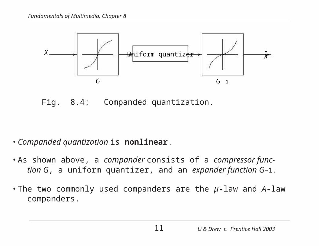
G −1
Uniform quantizerX^
X
G
Fig. 8.4: Companded quantization.
• Companded quantization is nonlinear.
• As shown above, a compander consists of a compressor func-tion G, a uniform quantizer, and an expander function G−1.
• The two commonly used companders are the µ-law and A-lawcompanders.
11 Li & Drew c Prentice Hall 2003
Fundamentals of Multimedia, Chapter 8
Vector Quantization (VQ)
• According to Shannon’s original work on information theory,any compression system performs better if it operates onvectors or groups of samples rather than individual symbolsor samples.
• Form vectors of input samples by simply concatenating anumber of consecutive samples into a single vector.
• Instead of single reconstruction values as in scalar quantiza-tion, in VQ code vectors with n components are used. Acollection of these code vectors form the codebook.
12 Li & Drew c Prentice Hall 2003
... ...
Fundamentals of Multimedia, Chapter 8
Index
Encoder
Find closestcode vector
Decoder
Table Lookup
X^X...
1
2
3
4
5
6
1
2
3
4
5
6
7
8
9
10
N
7
8
9
10
N
Fig. 8.5: Basic vector quantization procedure.
13 Li & Drew c Prentice Hall 2003
Fundamentals of Multimedia, Chapter 8
8.5 Transform Coding
• The rationale behind transform coding:
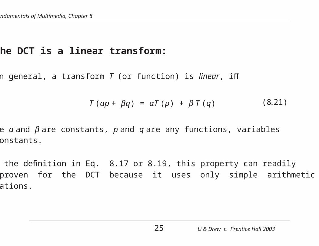
If Y is the result of a linear transform T of the input vectorX in such a way that the components of Y are much lesscorrelated, then Y can be coded more efficiently than X.
• If most information is accurately described by the first fewcomponents of a transformed vector, then the remainingcomponents can be coarsely quantized, or even set to zero,with little signal distortion.
• Discrete Cosine Transform (DCT) will be studied first. Inaddition, we will examine the Karhunen-Lo`eve Transform(KLT) which optimally decorrelates the components of the
input X.
14 Li & Drew c Prentice Hall 2003
Fundamentals of Multimedia, Chapter 8
Spatial Frequency and DCT
• Spatial frequency indicates how many times pixel valueschange across an image block.
• The DCT formalizes this notion with a measure of how muchthe image contents change in correspondence to the numberof cycles of a cosine wave per block.
• The role of the DCT is to decompose the original signalinto its DC and AC components; the role of the IDCT is toreconstruct (re-compose) the signal.
15 Li & Drew c Prentice Hall 2003
√
Fundamentals of Multimedia, Chapter 8
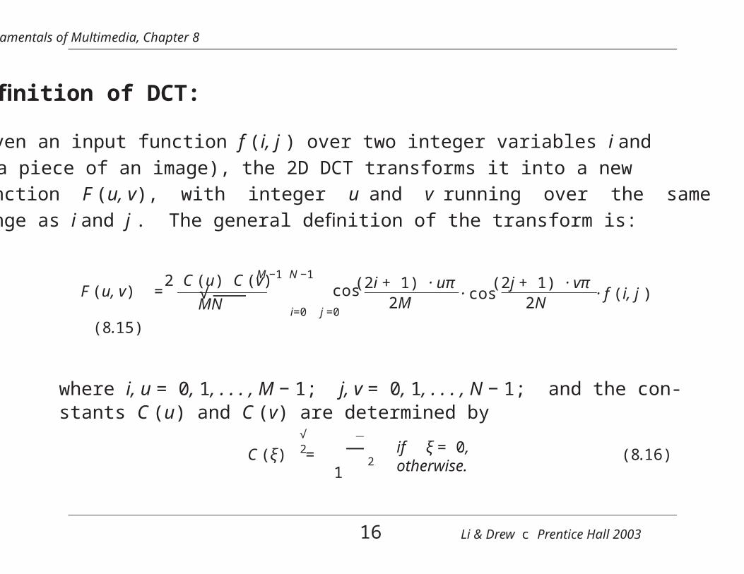
Definition of DCT:
Given an input function f (i, j ) over two integer variables i andj (a piece of an image), the 2D DCT transforms it into a newfunction F (u, v), with integer u and v running over the samerange as i and j . The general definition of the transform is:
F (u, v) =2 C (u) C (v)
MN
M −1 N −1
i=0 j =0
cos(2i + 1) · uπ2M
· cos(2j + 1) · vπ
2N· f (i, j )
(8.15)
where i, u = 0, 1, . . . , M − 1; j, v = 0, 1, . . . , N − 1; and the con-stants C (u) and C (v) are determined by
C (ξ) =√
22
1if ξ = 0,otherwise.
(8.16)
16 Li & Drew c Prentice Hall 2003
Fundamentals of Multimedia, Chapter 8
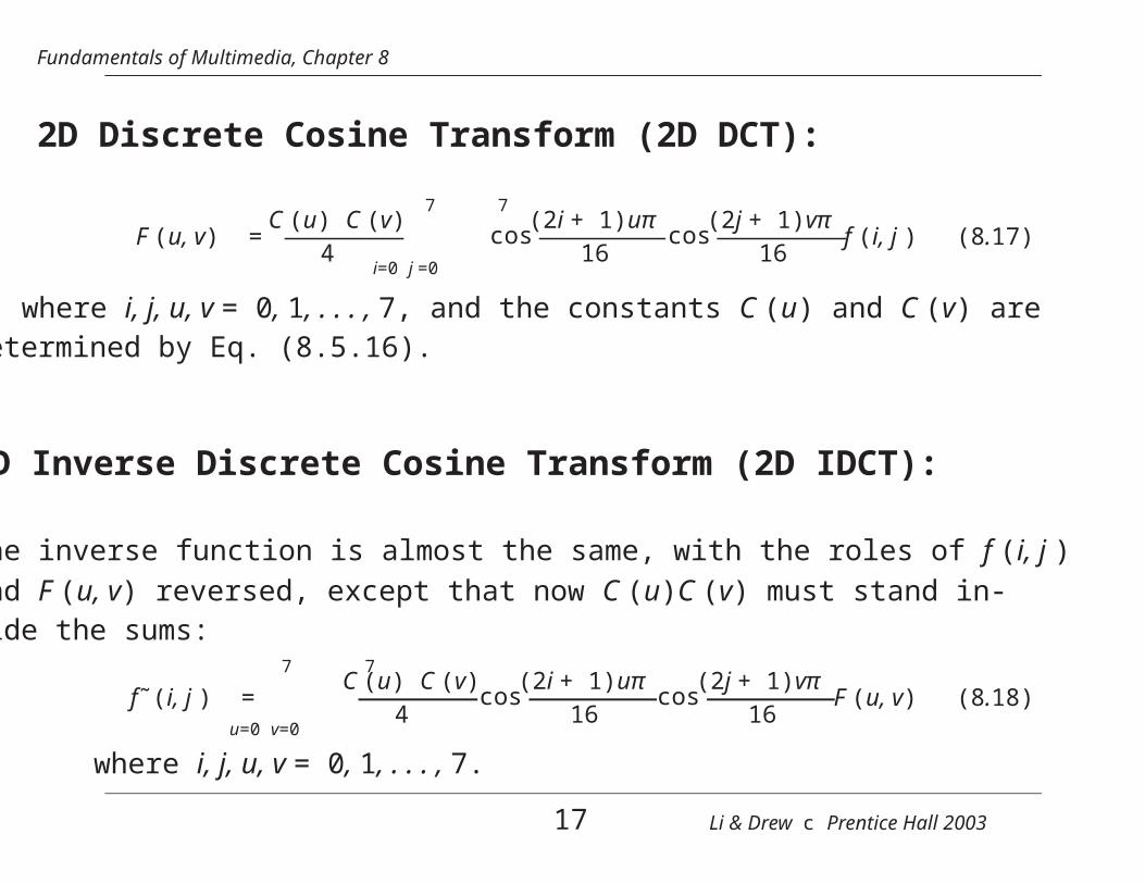
2D Discrete Cosine Transform (2D DCT):
F (u, v) =C (u) C (v)
4
7 7
i=0 j =0
cos(2i + 1)uπ
16cos
(2j + 1)vπ16
f (i, j ) (8.17)
where i, j, u, v = 0, 1, . . . , 7, and the constants C (u) and C (v) aredetermined by Eq. (8.5.16).
2D Inverse Discrete Cosine Transform (2D IDCT):
The inverse function is almost the same, with the roles of f (i, j )and F (u, v) reversed, except that now C (u)C (v) must stand in-side the sums:
f˜(i, j ) =7 7
u=0 v=0
C (u) C (v)4
cos(2i + 1)uπ
16cos
(2j + 1)vπ16
F (u, v) (8.18)
where i, j, u, v = 0, 1, . . . , 7.
17 Li & Drew c Prentice Hall 2003
Fundamentals of Multimedia, Chapter 8
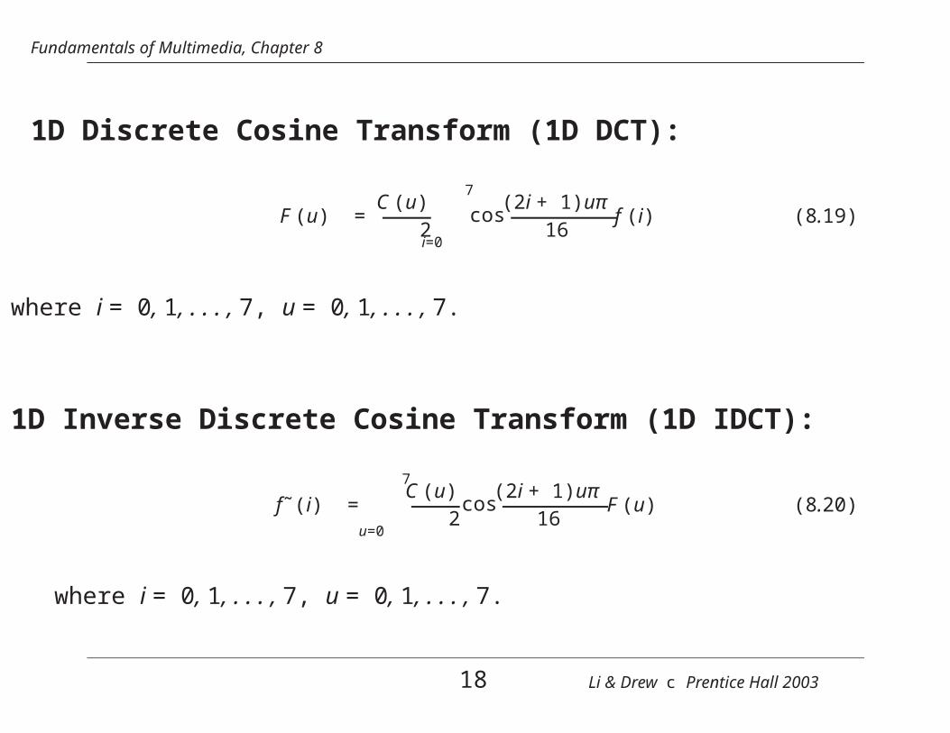
1D Discrete Cosine Transform (1D DCT):
F (u) =C (u)
2
7
i=0
cos(2i + 1)uπ
16f (i) (8.19)
where i = 0, 1, . . . , 7, u = 0, 1, . . . , 7.
1D Inverse Discrete Cosine Transform (1D IDCT):
f˜(i) =7
u=0
C (u)2
cos(2i + 1)uπ
16F (u) (8.20)
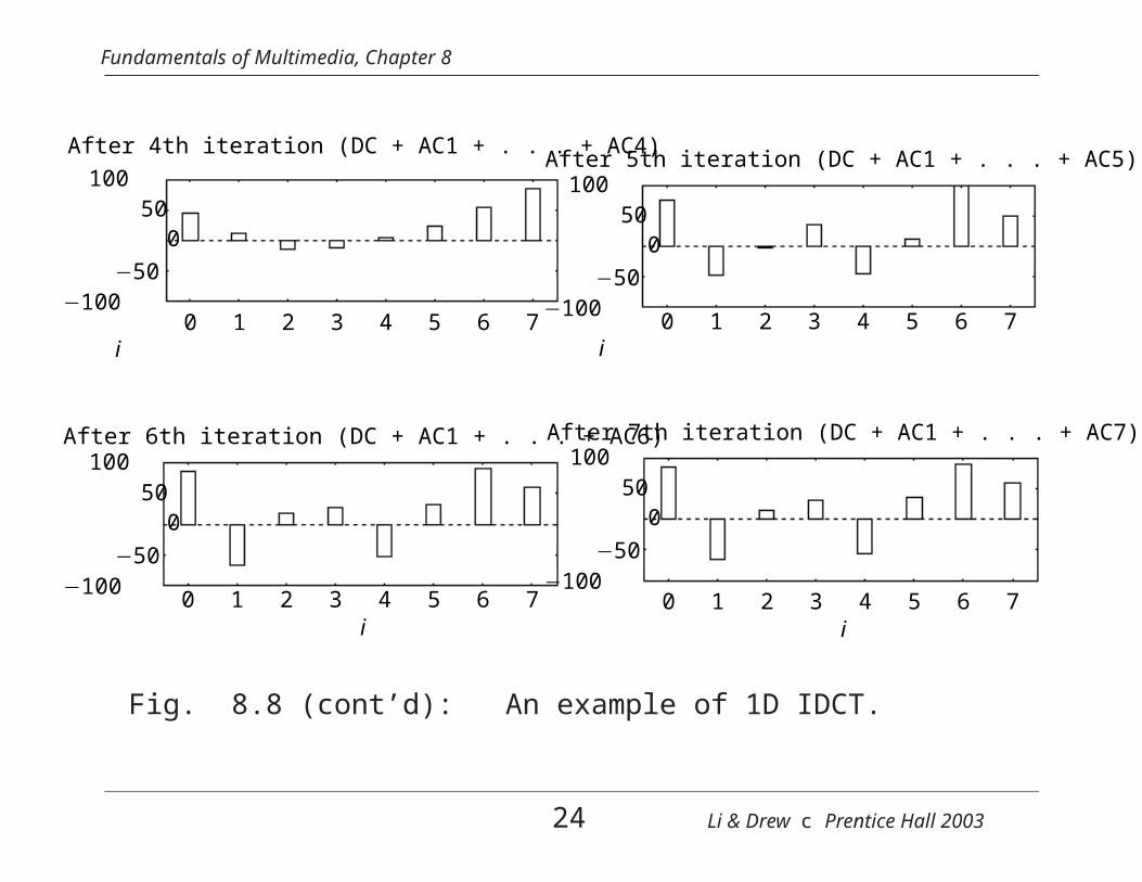
where i = 0, 1, . . . , 7, u = 0, 1, . . . , 7.
18 Li & Drew c Prentice Hall 2003
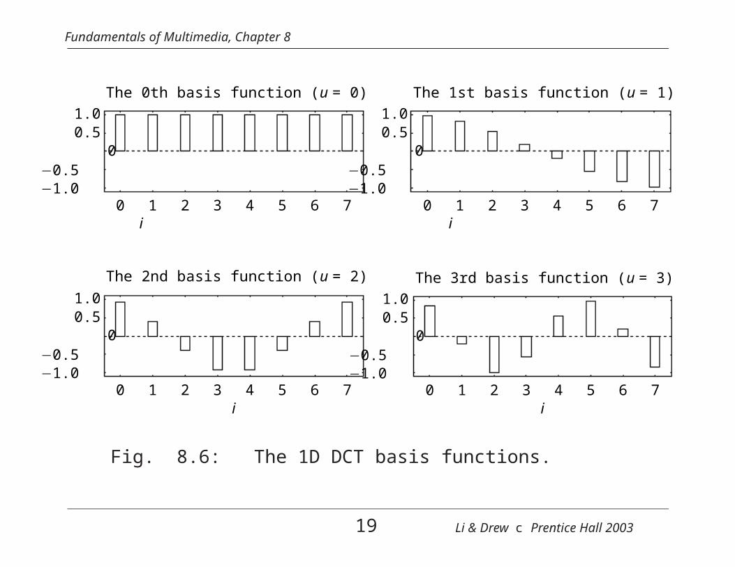
Fundamentals of Multimedia, Chapter 8
The 0th basis function (u = 0)
1.00.5
0−0.5−1.0
0 1 2 3 4 5 6 7
The 1st basis function (u = 1)
1.00.5
0−0.5−1.0
0 1 2 3 4 5 6 7i
The 2nd basis function (u = 2)
1.00.5
0−0.5−1.0
0 1 2 3 4 5 6 7i
i
The 3rd basis function (u = 3)
1.00.5
0−0.5−1.0
0 1 2 3 4 5 6 7i
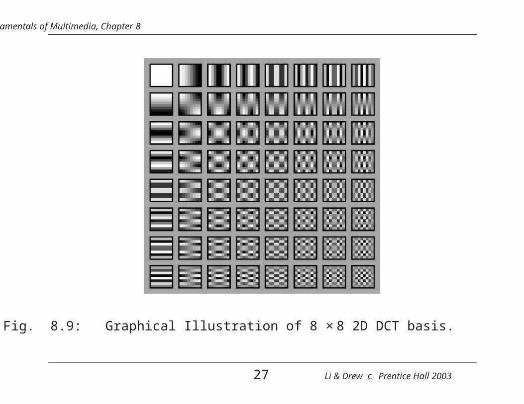
Fig. 8.6: The 1D DCT basis functions.
19 Li & Drew c Prentice Hall 2003
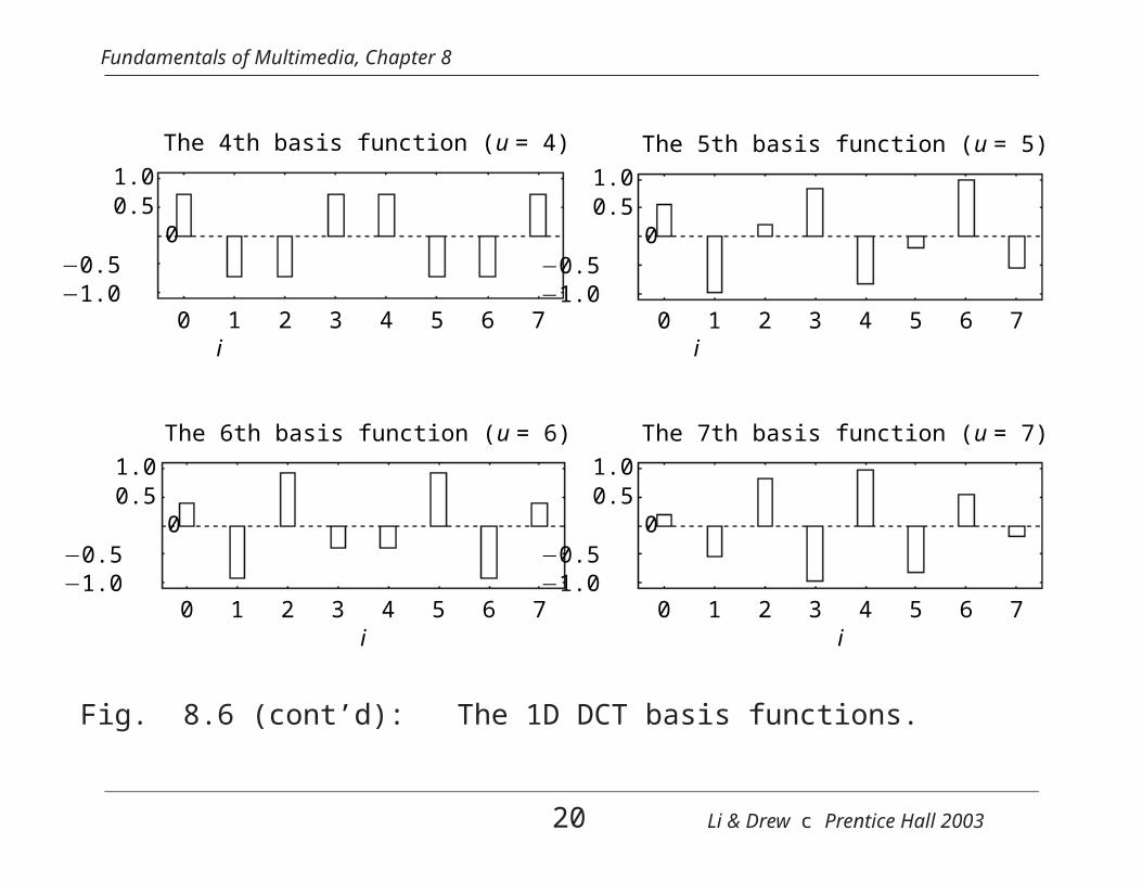
Fundamentals of Multimedia, Chapter 8
The 4th basis function (u = 4)
1.00.5
0−0.5−1.0
0 1 2 3 4 5 6 7
The 5th basis function (u = 5)
1.00.5
0−0.5−1.0
0 1 2 3 4 5 6 7i
The 6th basis function (u = 6)
1.00.5
0−0.5−1.0
0 1 2 3 4 5 6 7i
i
The 7th basis function (u = 7)
1.00.5
0−0.5−1.0
0 1 2 3 4 5 6 7i
Fig. 8.6 (cont’d): The 1D DCT basis functions.
20 Li & Drew c Prentice Hall 2003
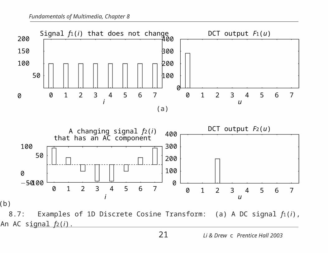
Fundamentals of Multimedia, Chapter 8
200
150
100
50
00 1 2 3 4 5 6 7
i
Signal f1(i) that does not change400
300
200
100
00 1 2 3 4 5 6 7
u
DCT output F1(u)
(a)
−100
10050
0
−50
0 1 2 3 4 5 6 7i
A changing signal f2(i)that has an AC component
0
400
300
200
100
0 1 2 3 4 5 6 7u
DCT output F2(u)
(b)
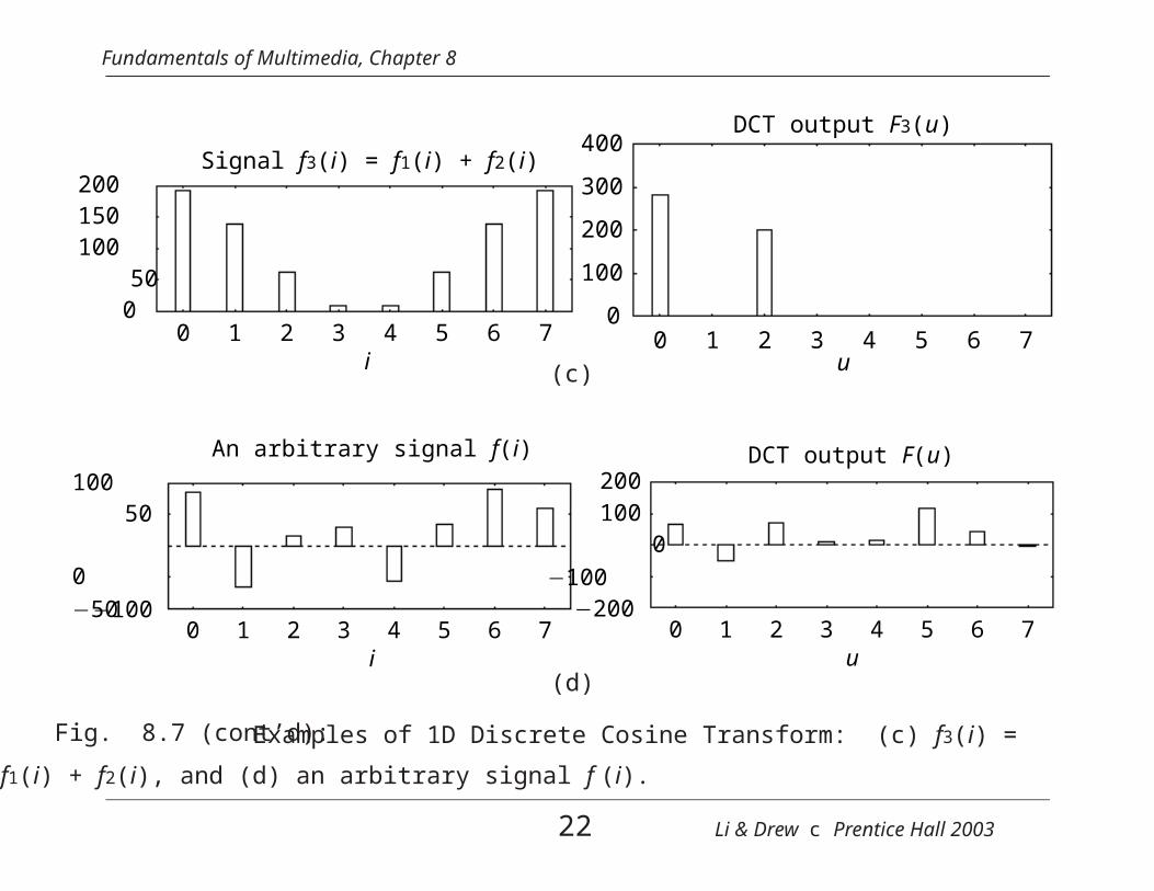
Fig. 8.7: Examples of 1D Discrete Cosine Transform: (a) A DC signal f1(i),(b) An AC signal f2(i).
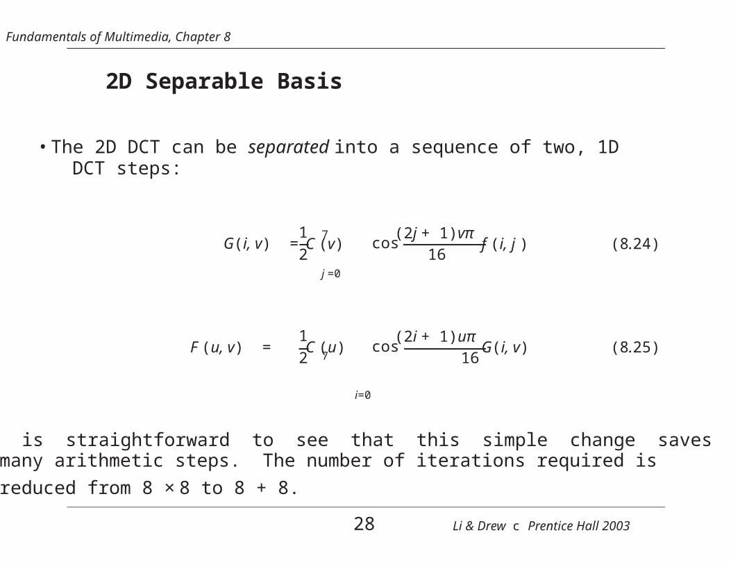
• The 2D DCT can be separated into a sequence of two, 1DDCT steps:
G(i, v) =
F (u, v) =
12
12
C (v)
C (u)
7
j =0
7
i=0
cos
cos
(2j + 1)vπ16
(2i + 1)uπ16
f (i, j )
G(i, v)
(8.24)
(8.25)
• It is straightforward to see that this simple change savesmany arithmetic steps. The number of iterations required is
reduced from 8 × 8 to 8 + 8.
28 Li & Drew c Prentice Hall 2003
fx · e
Fundamentals of Multimedia, Chapter 8
Comparison of DCT and DFT
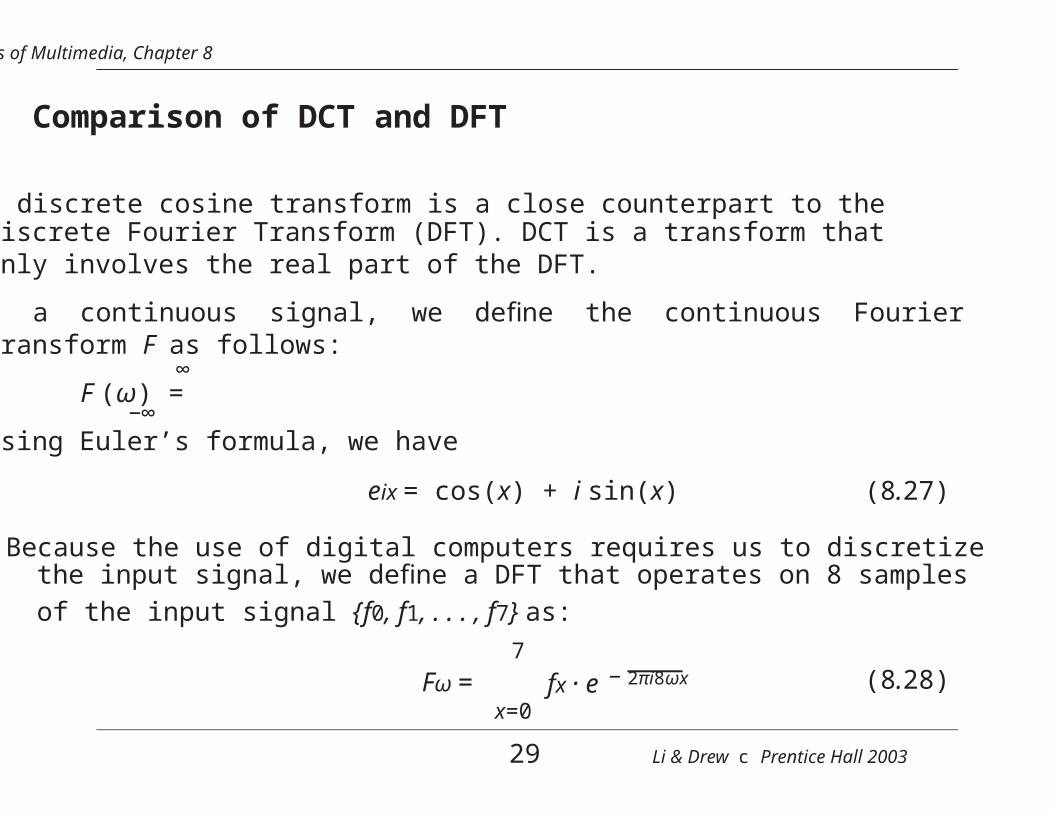
• The discrete cosine transform is a close counterpart to theDiscrete Fourier Transform (DFT). DCT is a transform thatonly involves the real part of the DFT.
• For a continuous signal, we define the continuous Fouriertransform F as follows:
∞F (ω) = (8.26)
−∞Using Euler’s formula, we have
eix = cos(x) + i sin(x) (8.27)
• Because the use of digital computers requires us to discretizethe input signal, we define a DFT that operates on 8 samplesof the input signal {f0, f1, . . . , f7} as:
Fω =7
x=0
− 2πi8ωx (8.28)
29 Li & Drew c Prentice Hall 2003
Fundamentals of Multimedia, Chapter 8
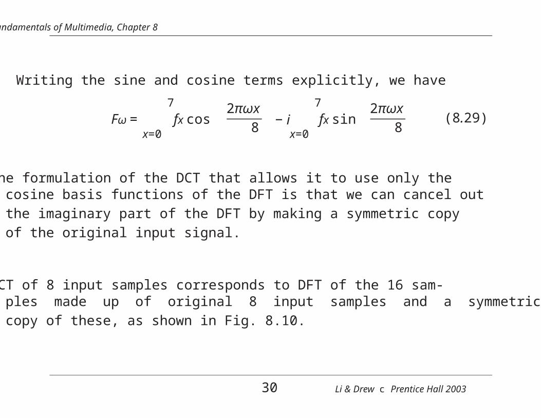
Writing the sine and cosine terms explicitly, we have
Fω =7
x=0fx cos
2πωx8− i
7
x=0fx sin
2πωx8
(8.29)
• The formulation of the DCT that allows it to use only thecosine basis functions of the DFT is that we can cancel outthe imaginary part of the DFT by making a symmetric copyof the original input signal.
• DCT of 8 input samples corresponds to DFT of the 16 sam-ples made up of original 8 input samples and a symmetriccopy of these, as shown in Fig. 8.10.
30 Li & Drew c Prentice Hall 2003
1 2 3 4 5 6 7 8 9 10 11 12 13 14 150
Fundamentals of Multimedia, Chapter 8
y
7
6
5
4
3
2
1
x
Fig. 8.10 Symmetric extension of the ramp function.
31 Li & Drew c Prentice Hall 2003
Fundamentals of Multimedia, Chapter 8
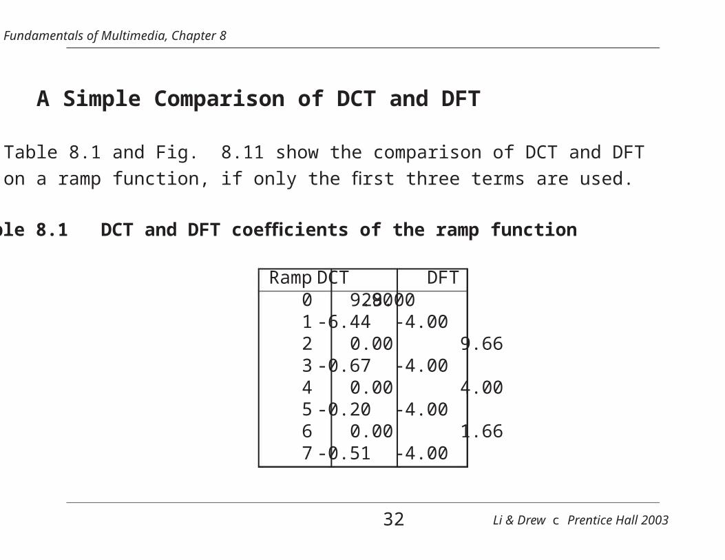
A Simple Comparison of DCT and DFT
Table 8.1 and Fig. 8.11 show the comparison of DCT and DFTon a ramp function, if only the first three terms are used.
Table 8.1 DCT and DFT coefficients of the ramp function
Ramp01234567
DCT9.90
-6.440.00
-0.670.00
-0.200.00
-0.51
32
DFT28.00
-4.009.66
-4.004.00
-4.001.66
-4.00
Li & Drew c Prentice Hall 2003
Fundamentals of Multimedia, Chapter 8
0
7
6
5
4
3
2
1
y
1 2 3 4 5 6 70
7
6
5
4
3
2
1
y
1 2 3 4 5 6 7x
(a)
x
(b)
Fig. 8.11: Approximation of the ramp function: (a) 3 TermDCT Approximation, (b) 3 Term DFT Approximation.
33 Li & Drew c Prentice Hall 2003
Fundamentals of Multimedia, Chapter 8
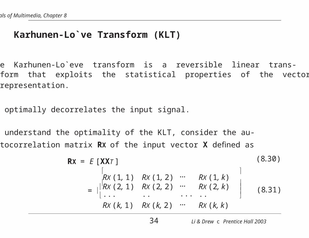
Karhunen-Lo`ve Transform (KLT)
• The Karhunen-Lo`eve transform is a reversible linear trans-form that exploits the statistical properties of the vectorrepresentation.
• It optimally decorrelates the input signal.
• To understand the optimality of the KLT, consider the au-
tocorrelation matrix RX of the input vector X defined as
RX = E [XXT ] (8.30)
=
RX (1, 1)RX (2, 1)...RX (k, 1)
RX (1, 2)RX (2, 2)..RX (k, 2)
······...···
RX (1, k)RX (2, k)..RX (k, k)
(8.31)
34 Li & Drew c Prentice Hall 2003
··· 0 ··· =
Fundamentals of Multimedia, Chapter 8
• Our goal is to find a transform T such that the componentsof the output Y are uncorrelated, i.e E [YtYs] = 0, if t = s.Thus, the autocorrelation matrix of Y takes on the form ofa positive diagonal matrix.
• Since any autocorrelation matrix is symmetric and non-negativedefinite, there are k orthogonal eigenvectors u1, u2, . . . , uk andk corresponding real and nonnegative eigenvalues λ1 ≥ λ2 ≥· · · ≥ λk ≥ 0.
• If we define the Karhunen-Lo`ve transform as
T = [u1, u2, · · · , uk ]T
• Then, the autocorrelation matrix of Y becomes
RY = E [YYT ] = E [TXXT T] = TRXTT
λ1 0 0λ2 0
0 ... ... 0 0 0 ··· λk
(8.32)
(8.35)
(8.36)
35 Li & Drew c Prentice Hall 2003
1 20 23
1
Fundamentals of Multimedia, Chapter 8
KLT Example
To illustrate the mechanics of the KLT, consider the four 3D
• Estimate the autocorrelation matrix of the input:
RX =
n
M i=1xixTi − mxmTx (8.37)
1.25 2.25 0.88
0.88 1.50 0.69
36 Li & Drew c Prentice Hall 2003
−0.4952 0.7456 = 0.4460
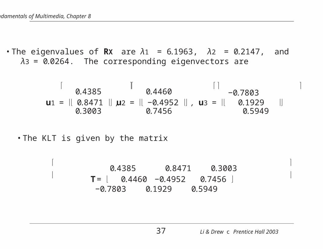
Fundamentals of Multimedia, Chapter 8
• The eigenvalues of RX are λ1 = 6.1963, λ2 = 0.2147, andλ3 = 0.0264. The corresponding eigenvectors are
0.4385
u1 = 0.8471 ,0.3003
0.4460
u2 = −0.4952 ,0.7456
−0.7803
u3 = 0.1929 0.5949
• The KLT is given by the matrix
T0.4385 0.8471 0.3003
−0.7803 0.1929 0.5949
37 Li & Drew c Prentice Hall 2003
Fundamentals of Multimedia, Chapter 8
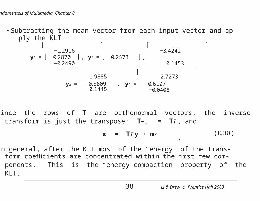
• Subtracting the mean vector from each input vector and ap-ply the KLT
−1.2916 −3.4242
y1 = −0.2870 , y2 = 0.2573 ,−0.2490 0.1453
1.9885
y3 = −0.5809 ,0.1445
2.7273
y4 = 0.6107 −0.0408
• Since the rows of T are orthonormal vectors, the inversetransform is just the transpose: T−1 = TT , and
x = TT y + mx (8.38)
• In general, after the KLT most of the “energy” of the trans-form coefficients are concentrated within the first few com-ponents. This is the “energy compaction” property of theKLT.
38 Li & Drew c Prentice Hall 2003
Fundamentals of Multimedia, Chapter 8
8.6 Wavelet-Based Coding
• The objective of the wavelet transform is to decompose theinput signal into components that are easier to deal with,have special interpretations, or have some components thatcan be thresholded away, for compression purposes.
• We want to be able to at least approximately reconstruct theoriginal signal given these components.
• The basis functions of the wavelet transform are localized inboth time and frequency.
• There are two types of wavelet transforms: the continuouswavelet transform (CWT) and the discrete wavelet transform(DWT).
39 Li & Drew c Prentice Hall 2003
ψs,u(t) = √ ψ
Fundamentals of Multimedia, Chapter 8
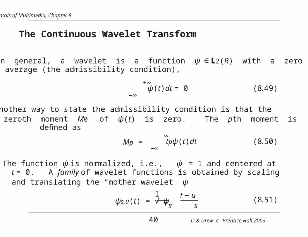
The Continuous Wavelet Transform
• In general, a wavelet is a function ψ ∈ L2(R) with a zeroaverage (the admissibility condition),
+∞
−∞ψ(t)dt = 0 (8.49)
• Another way to state the admissibility condition is that thezeroth moment M0 of ψ(t) is zero. The pth moment isdefined as
Mp =∞
−∞tpψ(t)dt (8.50)
• The function ψ is normalized, i.e., ψ = 1 and centered att = 0. A family of wavelet functions is obtained by scalingand translating the “mother wavelet” ψ
1
st − u
s(8.51)
40 Li & Drew c Prentice Hall 2003
W (f, s, u) √ ψ s
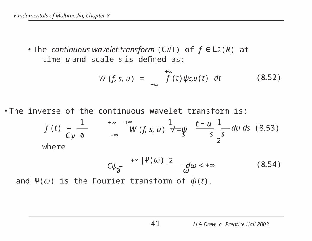
Fundamentals of Multimedia, Chapter 8
• The continuous wavelet transform (CWT) of f ∈ L2(R) attime u and scale s is defined as:
W (f, s, u) =+∞
−∞f (t)ψs,u(t) dt (8.52)
• The inverse of the continuous wavelet transform is:
f (t) =1 +∞
Cψ 0
+∞
−∞
1
st − u
s
12du ds (8.53)
where
Cψ =+∞ |Ψ(ω)|2
0 ωdω < +∞ (8.54)
and Ψ(ω) is the Fourier transform of ψ(t).
41 Li & Drew c Prentice Hall 2003
ψj,n(t) = √2
Fundamentals of Multimedia, Chapter 8
The Discrete Wavelet Transform
• Discrete wavelets are again formed from a mother wavelet,but with scale and shift in discrete steps.
• The DWT makes the connection between wavelets in thecontinuous time domain and “filter banks” in the discretetime domain in a multiresolution analysis framework.
• It is possible to show that the dilated and translated familyof wavelets ψ
1j
ψ t − 2j n2j (j,n)∈Z2
(8.55)
form an orthonormal basis of L2(R).
42 Li & Drew c Prentice Hall 2003
Fundamentals of Multimedia, Chapter 8
Multiresolution Analysis in the Wavelet Domain
• Multiresolution analysis provides the tool to adapt signal res-olution to only relevant details for a particular task.
The approximation component is then recursively decom-posed into approximation and detail at successively coarserscales.
• Wavelet functions ψ(t) are used to characterize detail infor-mation. The averaging (approximation) information is for-mally determined by a kind of dual to the mother wavelet,
called the “scaling function” φ(t).
• Wavelets are set up such that the approximation at resolution2−j contains all the necessary information to compute anapproximation at coarser resolution 2−(j +1).
43 Li & Drew c Prentice Hall 2003
Fundamentals of Multimedia, Chapter 8
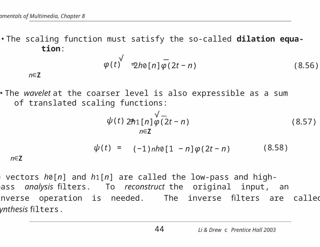
• The scaling function must satisfy the so-called dilation equa-tion:
φ(t) =√
2h0[n]φ(2t − n) (8.56)n∈Z
• The wavelet at the coarser level is also expressible as a sumof translated scaling functions:
ψ(t) =n∈Z
√2h1[n]φ(2t − n) (8.57)
ψ(t) = (−1)nh0[1 − n]φ(2t − n) (8.58)n∈Z
• The vectors h0[n] and h1[n] are called the low-pass and high-pass analysis filters. To reconstruct the original input, aninverse operation is needed. The inverse filters are calledsynthesis filters.
44 Li & Drew c Prentice Hall 2003
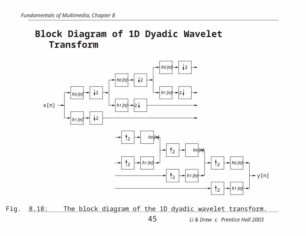
Fundamentals of Multimedia, Chapter 8
Block Diagram of 1D Dyadic WaveletTransform
x[n]
h1 [n]
h1 [n]
h0 [n]
h0 [n]
h0 [n]
h1 [n]
2
2
2
2
y[n]
2
h0 [n]
2
2
2
2
2
2
2
h0 [n]
h1 [n]
h1 [n] h0 [n]
h1 [n]
Fig. 8.18: The block diagram of the 1D dyadic wavelet transform.
45 Li & Drew c Prentice Hall 2003
Fundamentals of Multimedia, Chapter 8
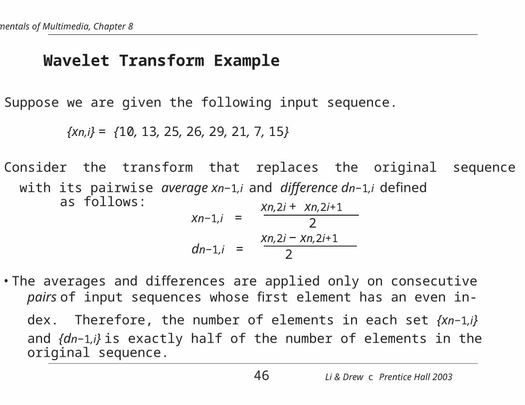
Wavelet Transform Example
• Suppose we are given the following input sequence.
{xn,i} = {10, 13, 25, 26, 29, 21, 7, 15}
• Consider the transform that replaces the original sequence
with its pairwise average xn−1,i and difference dn−1,i definedas follows:
xn−1,i =
dn−1,i =
xn,2i + xn,2i+1
2xn,2i − xn,2i+1
2
• The averages and differences are applied only on consecutivepairs of input sequences whose first element has an even in-
dex. Therefore, the number of elements in each set {xn−1,i}and {dn−1,i} is exactly half of the number of elements in theoriginal sequence.
46 Li & Drew c Prentice Hall 2003
Fundamentals of Multimedia, Chapter 8
• Form a new sequence having length equal to that of the orig-
inal sequence by concatenating the two sequences {xn−1,i}and {dn−1,i}. The resulting sequence is
• This sequence has exactly the same number of elements asthe input sequence — the transform did not increase theamount of data.
• Since the first half of the above sequence contain averagesfrom the original sequence, we can view it as a coarser ap-proximation to the original signal. The second half of thissequence can be viewed as the details or approximation errorsof the first half.
47 Li & Drew c Prentice Hall 2003
Fundamentals of Multimedia, Chapter 8
• It is easily verified that the original sequence can be recon-structed from the transformed sequence using the relations
xn,2i = xn−1,i + dn−1,i
xn,2i+1 = xn−1,i − dn−1,i
• This transform is the discrete Haar wavelet transform.
(b)
1.510
2
1
0
−1
2
1
0
−1
−2−0.5 1.510
−2−0.5
(a)
0.50.5
Fig. 8.12: Haar Transform: (a) scaling function, (b) wavelet function.
48 Li & Drew c Prentice Hall 2003
0 0 0 0 0 0 0 0
0 0 0 0 0 0 0 0
0 0 63 127 127 63 0 0
0 0 127 255 255 127 0 0
0 0 127 255 255 127 0 0
0 0 63 127 127 63 0 0
0 0 0 0 0 0 0 0
0 0 0 0 0 0 0 0
Fundamentals of Multimedia, Chapter 8
(a) (b)
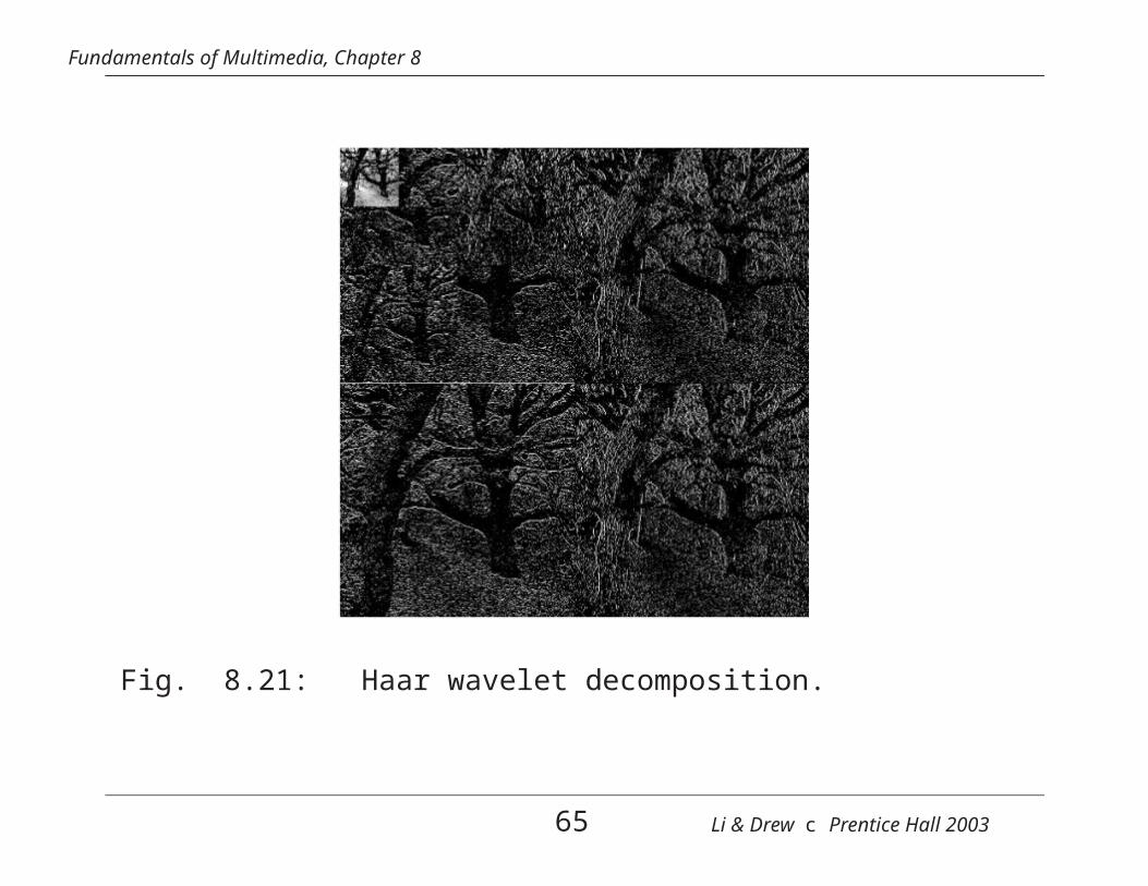
Fig. 8.13: Input image for the 2D Haar Wavelet Transform.
(a) The pixel values. (b) Shown as an 8 × 8 image.
49 Li & Drew c Prentice Hall 2003
0 0 0 0 0 0 0 0
0 0 0 0 0 0 0 0
0 95 95 0 0 −32 32 0
0 191 191 0 0 −64 64 0
0 191 191 0 0 −64 64 0
0 95 95 0 0 −32 32 0
0 0 0 0 0 0 0 0
0 0 0 0 0 0 0 0
Fundamentals of Multimedia, Chapter 8
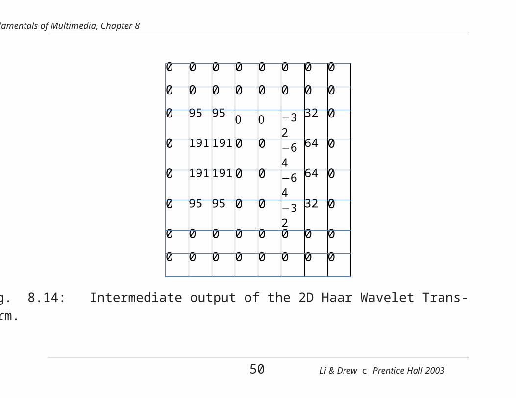
Fig. 8.14: Intermediate output of the 2D Haar Wavelet Trans-form.
50 Li & Drew c Prentice Hall 2003
0 0 0 0 0 0 0 0
0 143 143 0 0 −48 48 0
0 143 143 0 0 −48 48 0
0 0 0 0 0 0 0 0
0 0 0 0 0 0 0 0
0 −48 −48 0 0 16 −16 0
0 48 48 0 0 −16 16 0
0 0 0 0 0 0 0 0
Fundamentals of Multimedia, Chapter 8
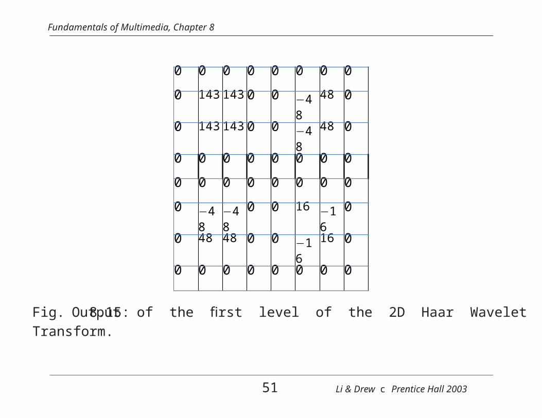
Output of the first level of the 2D Haar WaveletFig. 8.15:Transform.
51 Li & Drew c Prentice Hall 2003
Fundamentals of Multimedia, Chapter 8
Fig. 8.16: A simple graphical illustration of Wavelet Transform.
52 Li & Drew c Prentice Hall 2003
(t)
F(w
)
Fundamentals of Multimedia, Chapter 8
−10 −5 10
−1
3
2
1
0
0 5 −10 −5 100.0
3.0
2.0
1.0
0 5
Time
(a)
(a)
Frequency
(b)
(b)
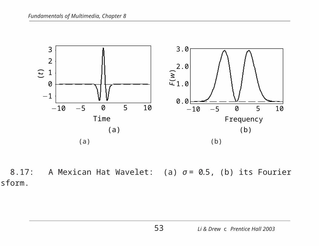
Fig. 8.17: A Mexican Hat Wavelet: (a) σ = 0.5, (b) its Fouriertransform.
53 Li & Drew c Prentice Hall 2003
Fundamentals of Multimedia, Chapter 8
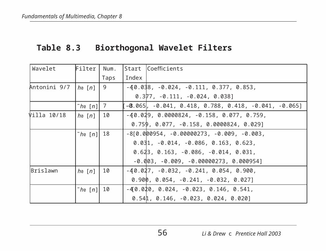
Biorthogonal Wavelets
• For orthonormal wavelets, the forward transform and its in-verse are transposes of each other and the analysis filters areidentical to the synthesis filters.
• Without orthogonality, the wavelets for analysis and synthe-sis are called “biorthogonal”. The synthesis filters are not
identical to the analysis filters. We denote them as ˜h0[n] and˜h1[n].
• To specify a biorthogonal wavelet transform, we require bothh0[n] and ˜h0[n].
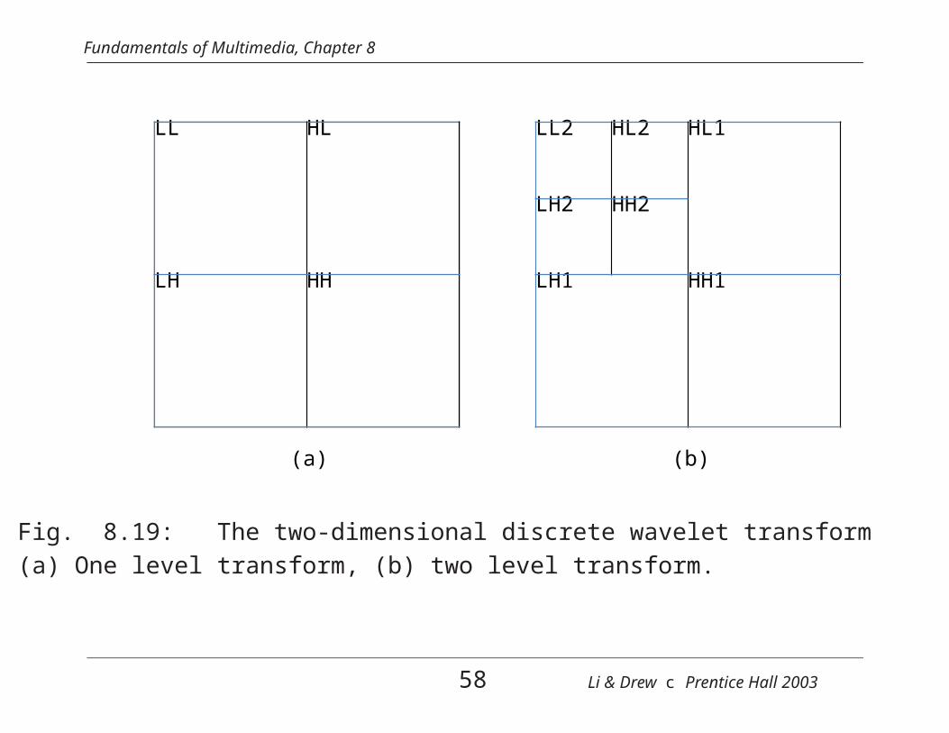
• For an N by N input image, the two-dimensional DWT pro-ceeds as follows:
– Convolve each row of the image with h0[n] and h1[n], discard the oddnumbered columns of the resulting arrays, and concatenate them toform a transformed row.
– After all rows have been transformed, convolve each column of theresult with h0[n] and h1[n]. Again discard the odd numbered rowsand concatenate the result.
• After the above two steps, one stage of the DWT is com-plete. The transformed image now contains four subbandsLL, HL, LH, and HH, standing for low-low, high-low, etc.
• The LL subband can be further decomposed to yield yet an-other level of decomposition. This process can be continueduntil the desired number of decomposition levels is reached.
57 Li & Drew c Prentice Hall 2003
LL HL
LH HH
LL2 HL2 HL1
LH2 HH2
LH1 HH1
Fundamentals of Multimedia, Chapter 8
(a) (b)
Fig. 8.19: The two-dimensional discrete wavelet transform(a) One level transform, (b) two level transform.
58 Li & Drew c Prentice Hall 2003
Fundamentals of Multimedia, Chapter 8
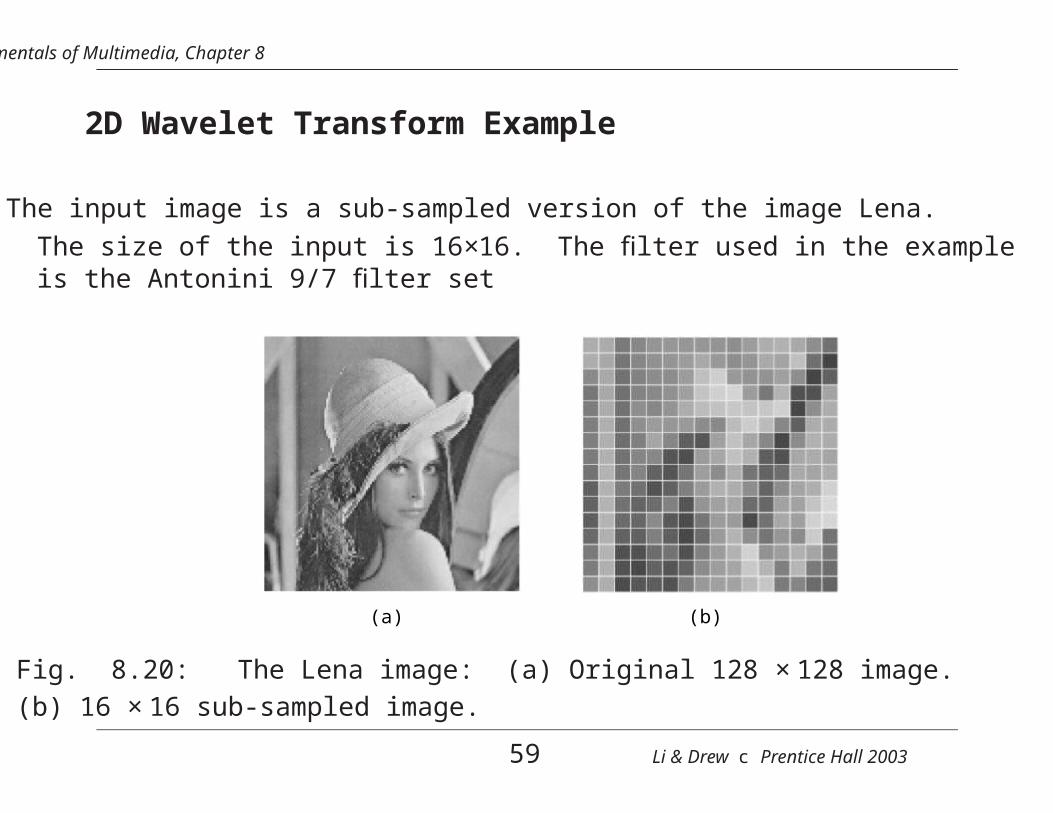
2D Wavelet Transform Example
• The input image is a sub-sampled version of the image Lena.The size of the input is 16×16. The filter used in the exampleis the Antonini 9/7 filter set
(b)(a)
Fig. 8.20: The Lena image: (a) Original 128 × 128 image.(b) 16 × 16 sub-sampled image.
59 Li & Drew c Prentice Hall 2003
Fundamentals of Multimedia, Chapter 8
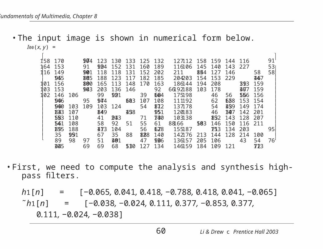
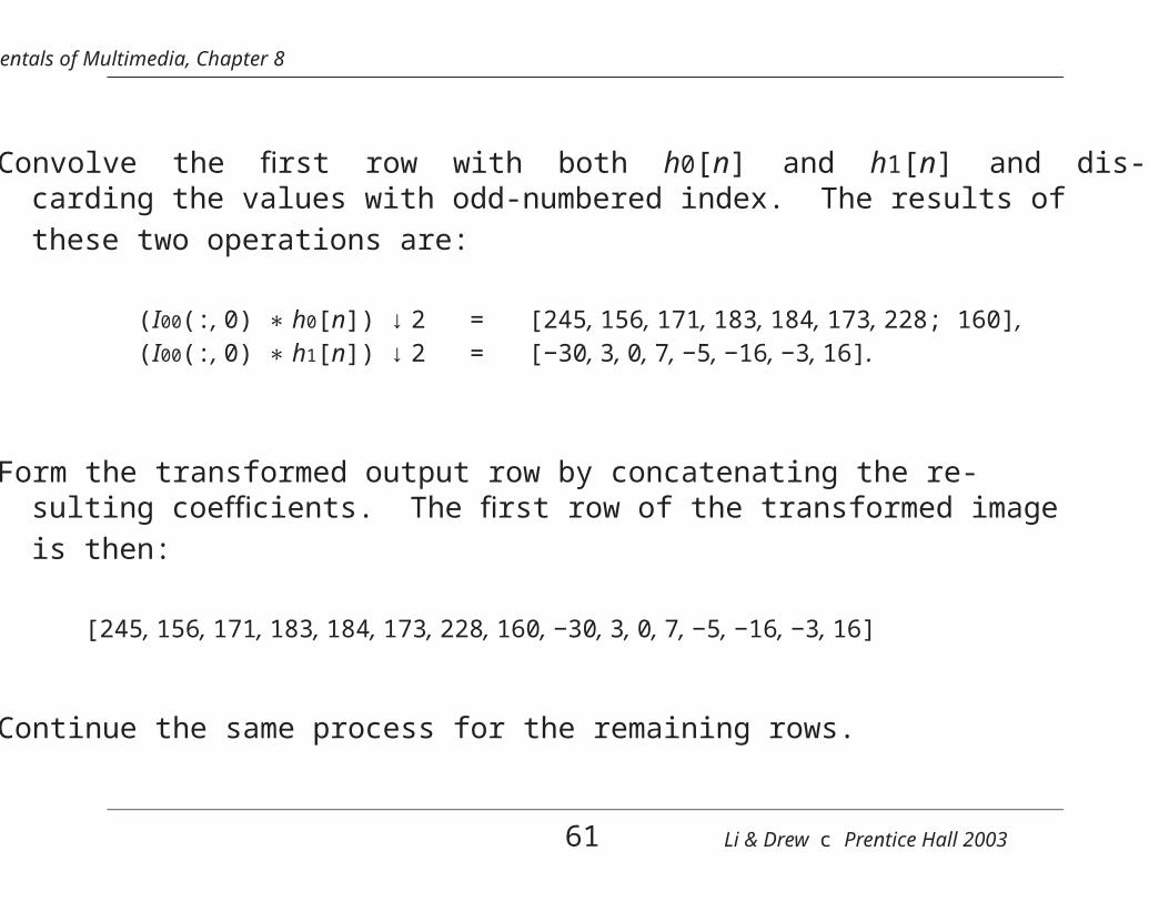
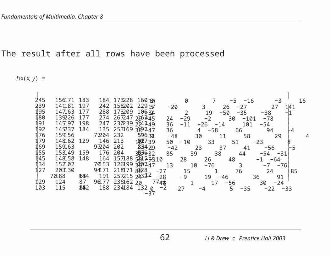
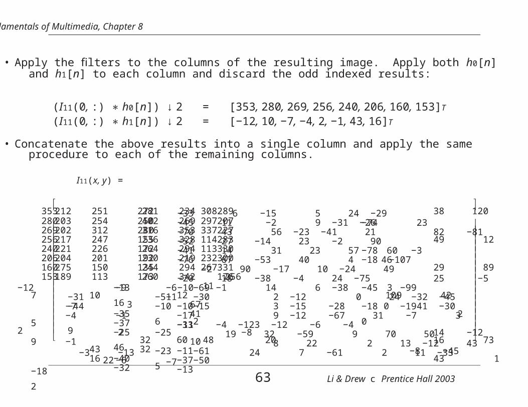
• The input image is shown in numerical form below.I00(x, y) =
158164116
95101103102
999984585689358944
170153149145156153146146140133153141115
9998
105
979190888994
10695
103107110108188151
9769
10499
101105100103
9997
10984415847675169
123124118188165203
99144103149
9492
113354968
130152118123113136121
61124
43213
51104
88101
53
133131131117148146
39103
54158
7155568847
110
125160152182170
9260
1078195736167
12890
127
132189202185163
66164108172151140
88128140136134
127116211204186192175111137120103166155142136146
112106
84203144188198192178183138
58187176157159
158145154154194103
4662544683
10371
213205184
159140127153208178
56654330
152146153144106109
144143146229
394756
128159147143150134128
43121
116227
5846
113167156153149142128116203214
5472
915358
147159159156154174201207211
95100
76113
• First, we need to compute the analysis and synthesis high-pass filters.
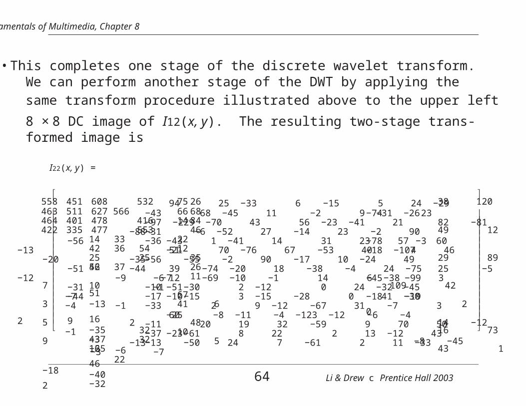
• This completes one stage of the discrete wavelet transform.We can perform another stage of the DWT by applying thesame transform procedure illustrated above to the upper left
8 × 8 DC image of I12(x, y). The resulting two-stage trans-formed image is
• In the usual dyadic wavelet decomposition, only the low-passfiltered subband is recursively decomposed and thus can berepresented by a logarithmic tree structure.
• A wavelet packet decomposition allows the decomposition tobe represented by any pruned subtree of the full tree topol-ogy.
• The wavelet packet decomposition is very flexible since abest wavelet basis in the sense of some cost metric can befound within a large library of permissible bases.
• The computational requirement for wavelet packet decom-position is relatively low as each decomposition can be com-puted in the order of N log N using fast filter banks.
66 Li & Drew c Prentice Hall 2003
Fundamentals of Multimedia, Chapter 8
8.8 Embedded Zerotree of Wavelet Coefficients
• Effective and computationally efficient for image coding.
• The EZW algorithm addresses two problems:
1. obtaining the best image quality for a given bit-rate, and
2. accomplishing this task in an embedded fashion.
• Using an embedded code allows the encoder to terminate theencoding at any point. Hence, the encoder is able to meetany target bit-rate exactly.
• Similarly, a decoder can cease to decode at any point andcan produce reconstructions corresponding to all lower-rateencodings.
67 Li & Drew c Prentice Hall 2003
Fundamentals of Multimedia, Chapter 8
The Zerotree Data Structure
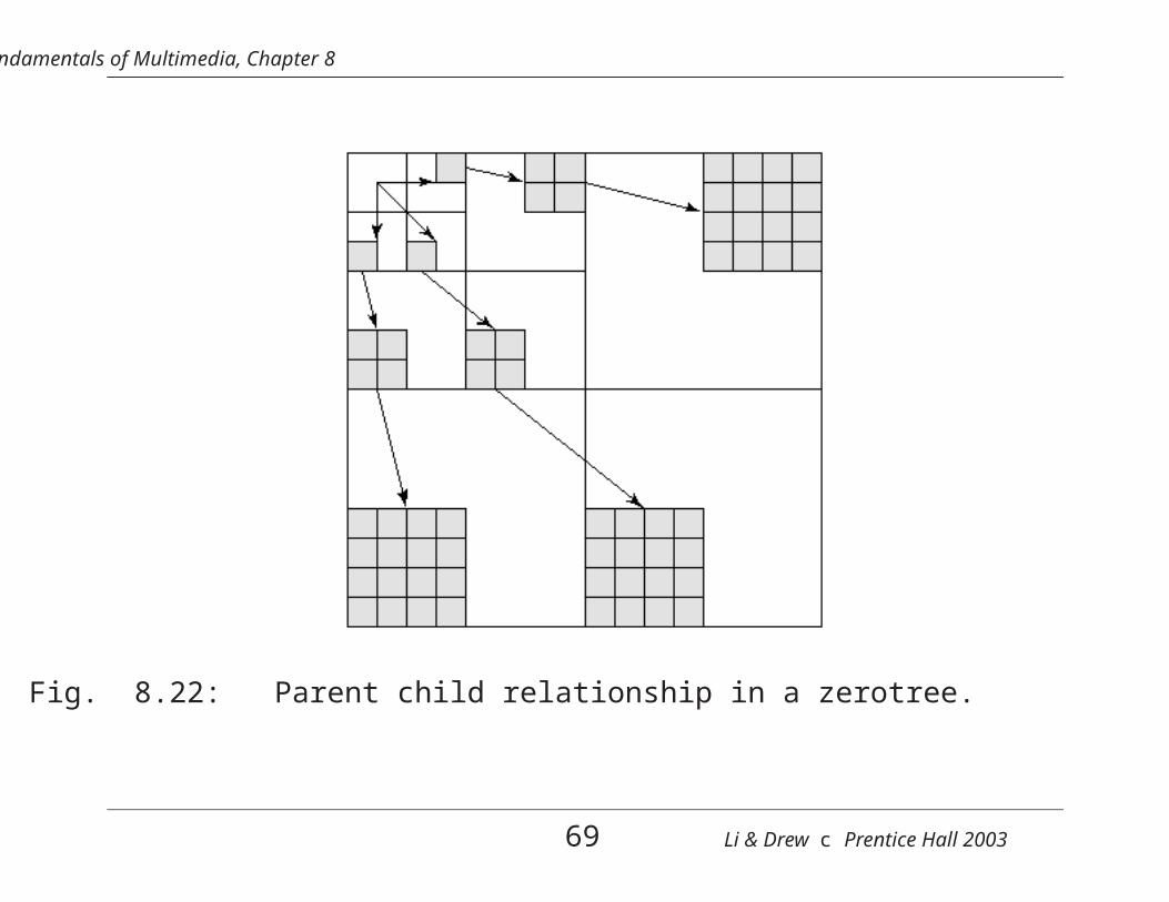
• The EZW algorithm efficiently codes the “significance map”which indicates the locations of nonzero quantized waveletcoefficients.
This is is achieved using a new data structure called thezerotree.
• Using the hierarchical wavelet decomposition presented ear-lier, we can relate every coefficient at a given scale to a setof coefficients at the next finer scale of similar orientation.
• The coefficient at the coarse scale is called the “parent”while all corresponding coefficients are the next finer scale ofthe same spatial location and similar orientation are called“children”.
68 Li & Drew c Prentice Hall 2003
Fundamentals of Multimedia, Chapter 8
Fig. 8.22: Parent child relationship in a zerotree.
69 Li & Drew c Prentice Hall 2003
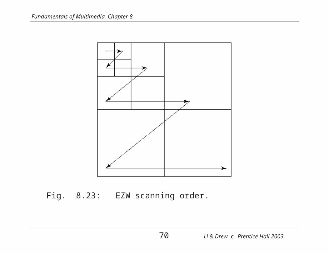
Fundamentals of Multimedia, Chapter 8
Fig. 8.23: EZW scanning order.
70 Li & Drew c Prentice Hall 2003
Fundamentals of Multimedia, Chapter 8
• Given a threshold T , a coefficient x is an element of thezerotree if it is insignificant and all of its descendants areinsignificant as well.
• The significance map is coded using the zerotree with a four-symbol alphabet:
– The zerotree root: The root of the zerotree is encodedwith a special symbol indicating that the insignificance ofthe coefficients at finer scales is completely predictable.
– Isolated zero: The coefficient is insignificant but hassome significant descendants.
– Positive significance: The coefficient is significant witha positive value.
– Negative significance: The coefficient is significant witha negative value.
71 Li & Drew c Prentice Hall 2003
Fundamentals of Multimedia, Chapter 8
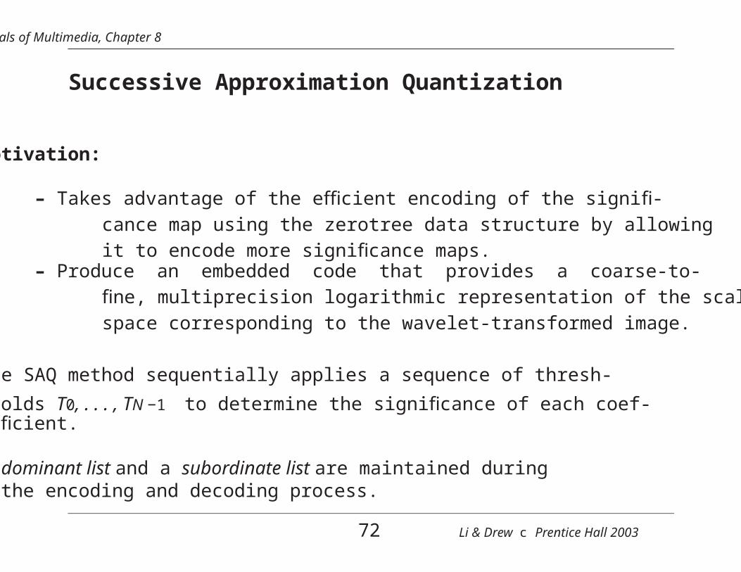
Successive Approximation Quantization
• Motivation:
– Takes advantage of the efficient encoding of the signifi-cance map using the zerotree data structure by allowingit to encode more significance maps.
– Produce an embedded code that provides a coarse-to-fine, multiprecision logarithmic representation of the scalespace corresponding to the wavelet-transformed image.
• The SAQ method sequentially applies a sequence of thresh-
olds T0, . . . , TN −1 to determine the significance of each coef-ficient.
• A dominant list and a subordinate list are maintained duringthe encoding and decoding process.
72 Li & Drew c Prentice Hall 2003
Fundamentals of Multimedia, Chapter 8
Dominant Pass
• Coefficients having their coordinates on the dominant listimplies that they are not yet significant.
• Coefficients are compared to the threshold Ti to determinetheir significance. If a coefficient is found to be significant,its magnitude is appended to the subordinate list and thecoefficient in the wavelet transform array is set to 0 to en-able the possibility of the occurrence of a zerotree on futuredominant passes at smaller thresholds.
• The resulting significance map is zerotree coded.
73 Li & Drew c Prentice Hall 2003
Fundamentals of Multimedia, Chapter 8
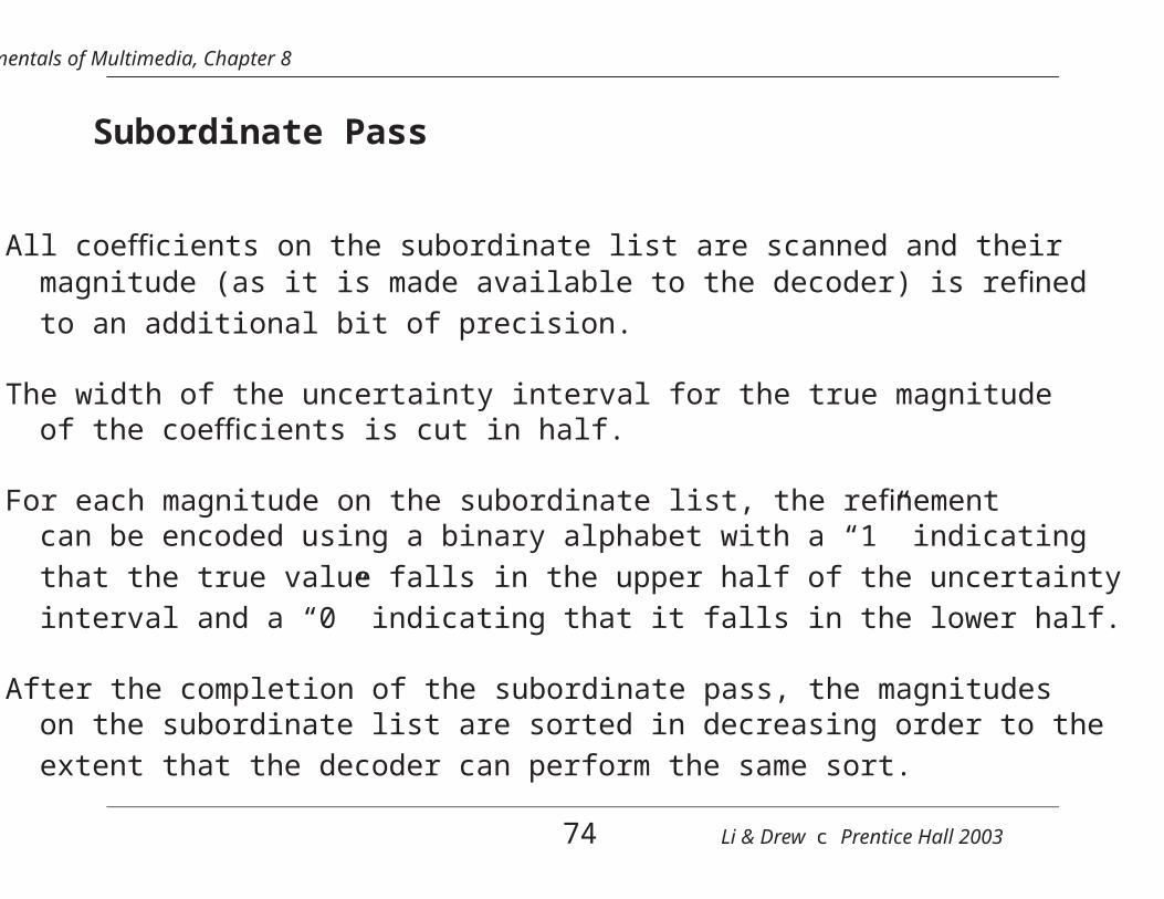
Subordinate Pass
• All coefficients on the subordinate list are scanned and theirmagnitude (as it is made available to the decoder) is refinedto an additional bit of precision.
• The width of the uncertainty interval for the true magnitudeof the coefficients is cut in half.
• For each magnitude on the subordinate list, the refinementcan be encoded using a binary alphabet with a “1” indicatingthat the true value falls in the upper half of the uncertaintyinterval and a “0” indicating that it falls in the lower half.
• After the completion of the subordinate pass, the magnitudeson the subordinate list are sorted in decreasing order to theextent that the decoder can perform the same sort.
74 Li & Drew c Prentice Hall 2003
57 −37
39 −20
17 33
3 7 9 10
8 2 1 6
9 −4 2 3
−7 14 12 −9
−29
30
14 6
10 19
15 13
−7 9
12 15 33 20
0 7 2 4
4 1 10 3
5 6 0 0
−2 3 1 0
4
−1 1 1
2 0 1 0
3 1 2 1
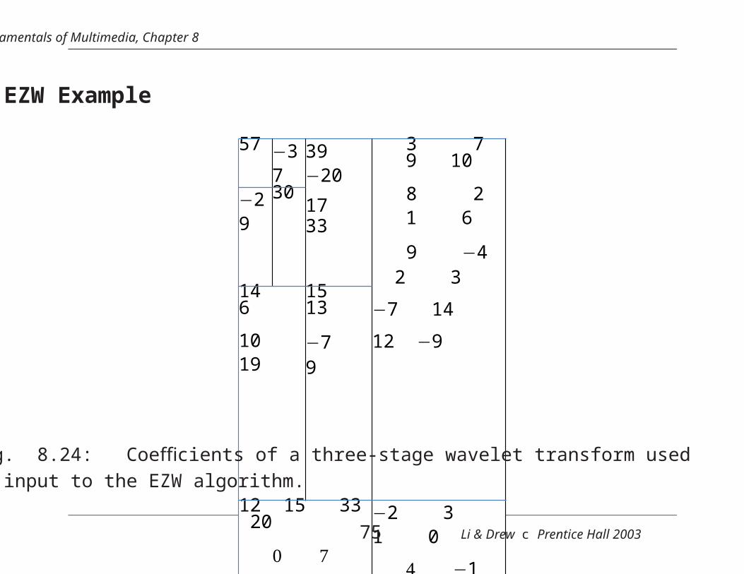
Fundamentals of Multimedia, Chapter 8
EZW Example
Fig. 8.24: Coefficients of a three-stage wavelet transform usedas input to the EZW algorithm.
75 Li & Drew c Prentice Hall 2003
Fundamentals of Multimedia, Chapter 8
Encoding
• Since the largest coefficient is 57, the initial threshold T0 is32.
• At the beginning, the dominant list contains the coordinatesof all the coefficients.
• The following is the list of coefficients visited in the order ofthe scan:
{57, −37, −29, 30, 39, −20, 17, 33, 14, 6, 10,
19, 3, 7, 8, 2, 2, 3, 12, −9, 33, 20, 2, 4}
• With respect to the threshold T0 = 32, it is easy to see thatthe coefficients 57 and -37 are significant. Thus, we output
a p and a n to represent them.
76 Li & Drew c Prentice Hall 2003
Fundamentals of Multimedia, Chapter 8
• The coefficient −29 is insignificant, but contains a significantdescendant 33 in LH1. Therefore, it is coded as z.
• Continuing in this manner, the dominant pass outputs thefollowing symbols:
D0 : pnztpttptzttttttttttpttt
• There are five coefficients found to be significant: 57, -37,39, 33, and another 33. Since we know that no coefficients
are greater than 2T0 = 64 and the threshold used in the firstdominant pass is 32, the uncertainty interval is thus [32, 64).
• The subordinate pass following the dominant pass refines themagnitude of these coefficients by indicating whether they liein the first half or the second half of the uncertainty interval.
S0 : 10000
77 Li & Drew c Prentice Hall 2003
Fundamentals of Multimedia, Chapter 8
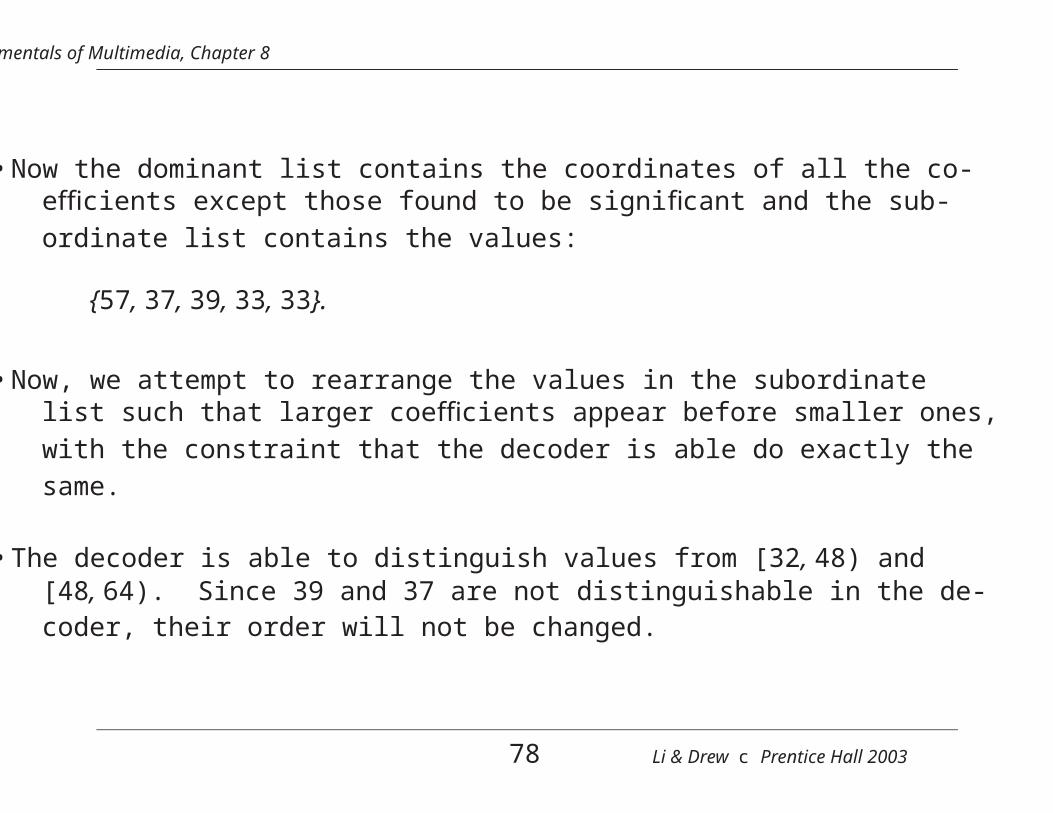
• Now the dominant list contains the coordinates of all the co-efficients except those found to be significant and the sub-ordinate list contains the values:
{57, 37, 39, 33, 33}.
• Now, we attempt to rearrange the values in the subordinatelist such that larger coefficients appear before smaller ones,with the constraint that the decoder is able do exactly thesame.
• The decoder is able to distinguish values from [32, 48) and[48, 64). Since 39 and 37 are not distinguishable in the de-coder, their order will not be changed.
78 Li & Drew c Prentice Hall 2003
Fundamentals of Multimedia, Chapter 8
• Before we move on to the second round of dominant andsubordinate passes, we need to set the values of the signifi-cant coefficients to 0 in the wavelet transform array so thatthey do not prevent the emergence of a new zerotree.
• The new threshold for second dominant pass is T1 = 16. Us-ing the same procedure as above, the dominant pass outputsthe following symbols
(8.65)D1 : zznptnpttztptttttttttttttptttttt
• The subordinate list is now:
{57, 37, 39, 33, 33, 29, 30, 20, 17, 19, 20}
79 Li & Drew c Prentice Hall 2003
Fundamentals of Multimedia, Chapter 8
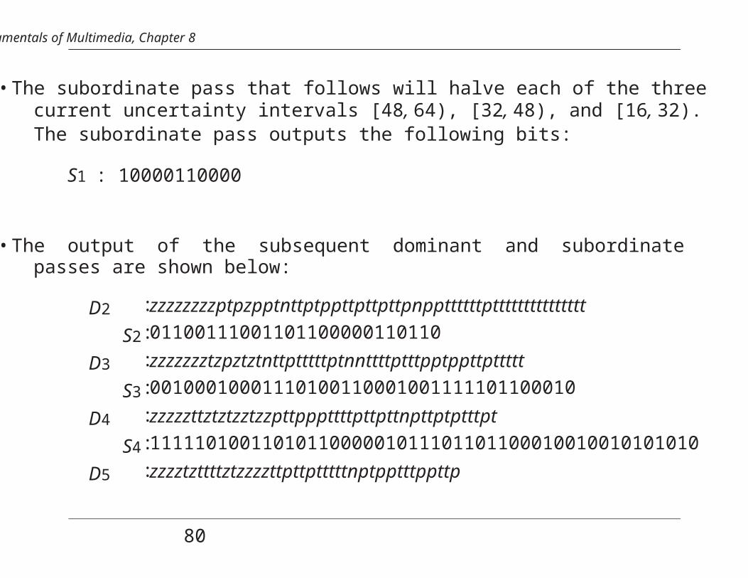
• The subordinate pass that follows will halve each of the threecurrent uncertainty intervals [48, 64), [32, 48), and [16, 32).The subordinate pass outputs the following bits:
S1 : 10000110000
• The output of the subsequent dominant and subordinatepasses are shown below:
• Suppose we only received information from the first dominantand subordinate pass. From the symbols in D0 we can obtainthe position of the significant coefficients. Then, using the
bits decoded from S0, we can reconstruct the value of thesecoefficients using the center of the uncertainty interval.
Fig. 8.25: Reconstructed transform coefficients from the first pass.
81 Li & Drew c Prentice Hall 2003
58
12
-38
0
38
12
-22
12
0 0 12 12
0 0 0
12 0 0 012 20 0 12 0 12 12 -12
12 12 34 22 0 0 0 0
0 0 0 0
0 0 0 0
0 0 0 0
0 0 0 0
0 0 12 0
0 0 0 0
Fundamentals of Multimedia, Chapter 8
• If the decoder received only D0, S0, D1, S1, D2, and only thefirst 10 bits of S2, then the reconstruction is
Fig. 8.26: Reconstructed transform coefficients from D0,S0, D1, S1, D2, and the first 10 bits of S2 .
82 Li & Drew c Prentice Hall 2003
Fundamentals of Multimedia, Chapter 8
8.9 Set Partitioning in Hierarchical Trees(SPIHT)
• The SPIHT algorithm is an extension of the EZW algorithm.
• The SPIHT algorithm significantly improved the performanceof its predecessor by changing the way subsets of coefficientsare partitioned and how refinement information is conveyed.
• A unique property of the SPIHT bitstream is its compact-ness. The resulting bitstream from the SPIHT algorithm isso compact that passing it through an entropy coder wouldonly produce very marginal gain in compression.
• No ordering information is explicitly transmitted to the de-coder. Instead, the decoder reproduces the execution pathof the encoder and recovers the ordering information.
83 Li & Drew c Prentice Hall 2003
Fundamentals of Multimedia, Chapter 8
8.10 Further Explorations
• Text books:
– Introduction to Data Compression by Khalid Sayood
– Vector Quantization and Signal Compression by Allen Gersho andRobert M. Gray
– Digital Image Processing by Rafael C. Gonzales and Richard E. Woods
– Probability and Random Processes with Applications to Signal Pro-cessing by Henry Stark and John W. Woods
– A Wavelet Tour of Signal Processing by Stephane G. Mallat
• Web sites:−→ Link to Further Exploration for Chapter 8.. including:
– An online graphics-based demonstration of the wavelet transform.
– Links to documents and source code related to quantization, Theoryof Data Compression webpage, FAQ for comp.compression, etc.
– A link to an excellent article Image Compression – from DCT toWavelets : A Review.


![Successive Lossy Compression for Laplacian Sourcesyoungsuk/papers/report_lossycompression.pdf · Gaussian source. For a Laplacian source, MCMC based compressor [7] in high distortion](https://static.documents.pub/doc/80x56/5c8ca33b09d3f236358c32ae/successive-lossy-compression-for-laplacian-sources-youngsukpapersreportlossycompressionpdf.jpg)


