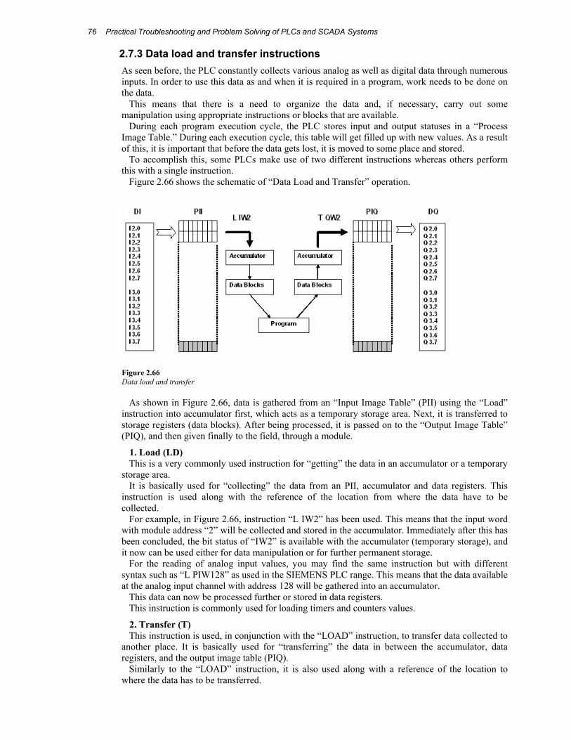
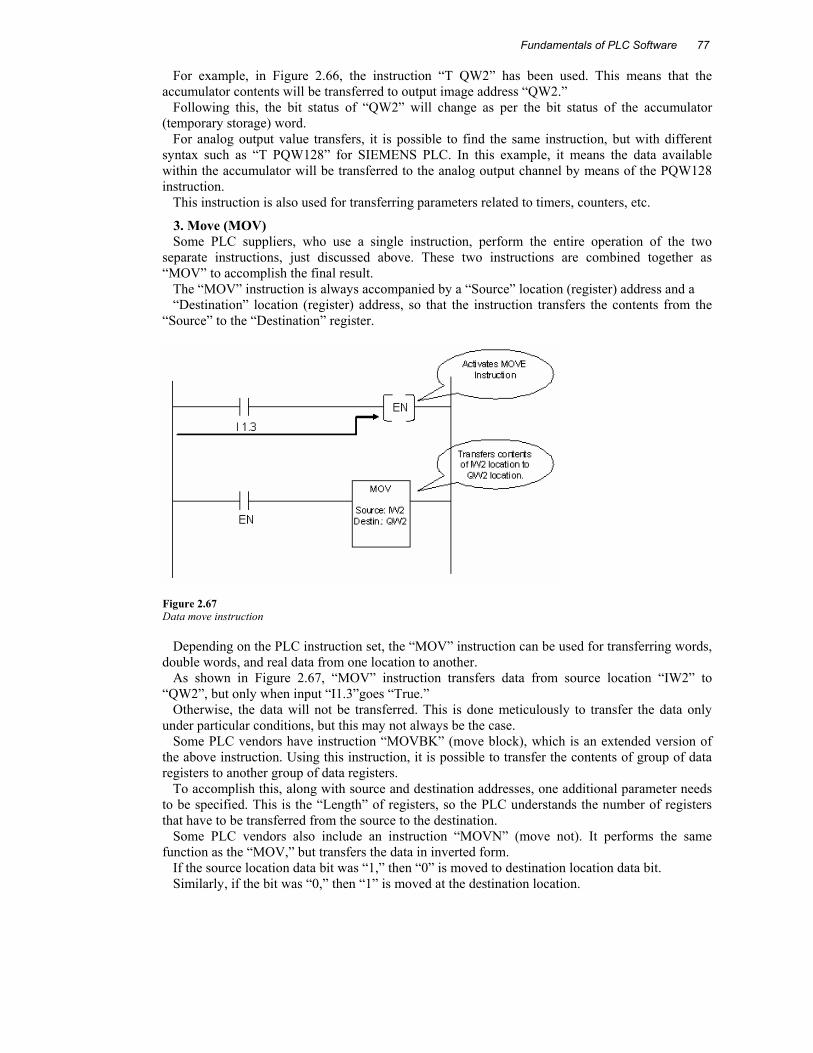
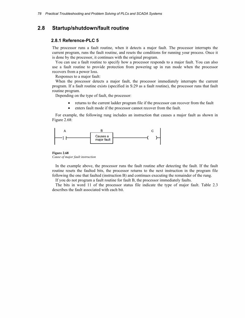
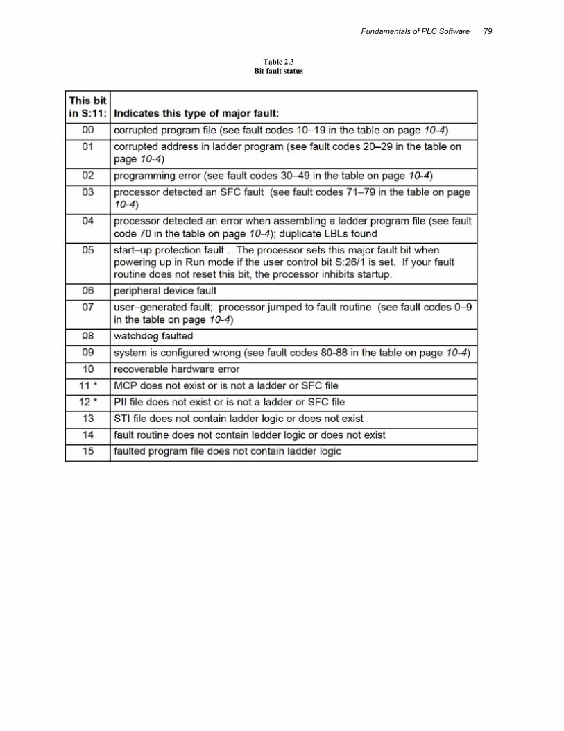
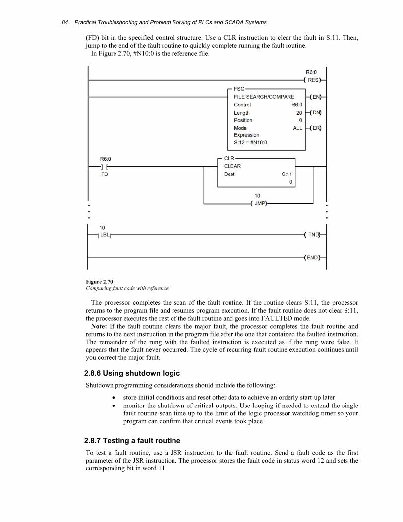
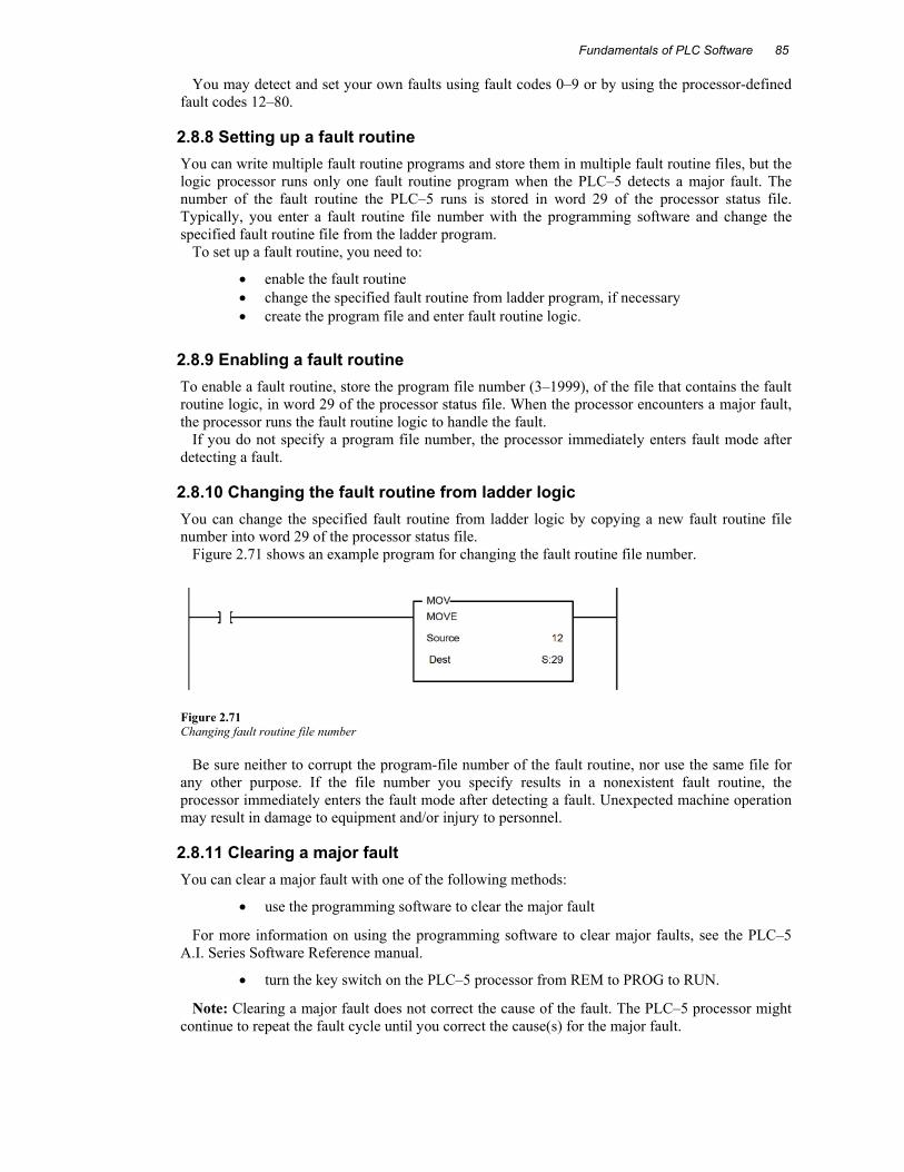
Fundamentals of PLC Software · Fundamentals of PLC Software 37 The “L1” and “L2”...

2

Fundamentals of PLC Software

2.1 Introduction A programmable logic controller (PLC) is a device that was invented to replace the necessary sequential electrical relay circuits for machine control. The PLC works by looking at its inputs and depending upon their state, turning on/off its outputs. The user enters a program, usually via software, that gives the desired results.

For example, a switch turns on a solenoid for 5 s and then turns it off. We can do this with a simple external timer. But what if the process included 10 switches and 10 solenoids? We would need 10 external timers.

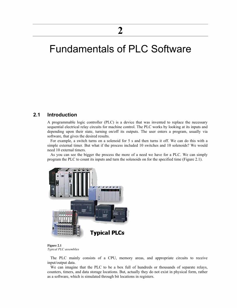
As you can see the bigger the process the more of a need we have for a PLC. We can simply program the PLC to count its inputs and turn the solenoids on for the specified time (Figure 2.1).

Figure 2.1 Typical PLC assemblies

The PLC mainly consists of a CPU, memory areas, and appropriate circuits to receive input/output data.

We can imagine that the PLC to be a box full of hundreds or thousands of separate relays, counters, timers, and data storage locations. But, actually they do not exist in physical form, rather as a software, which is simulated through bit locations in registers.

Practical Troubleshooting and Problem Solving of PLCs and SCADA Systems 36

What is inside the PLC?

• Input relays – (contacts) These are connected to the outside world. They physically exist and receive signals from switches, sensors, etc. Typically they are not relays but rather they are transistors.

• Internal utility relays – (contacts) These do not receive signals neither from the outside world nor do they physically exist. They are simulated relays and are what enables a PLC to eliminate external relays. There are also some special relays that are dedicated to performing only one task. Some are always switched on while some are always switched off. Some are on only once during the power is on and are typically used for initializing data that were stored.

• Counters – These again do not physically exist. They are simulated counters and they can be programmed to count pulses. Typically, these counters can count up, down, or both up and down. Since they are simulated, they are limited in their counting speed. Some manufacturers also include high-speed counters that are hardware based. We can think of these as physically existing. Most times, these counters can count up, down, or up and down.

• Timers – These also do not physically exist. They come in many varieties and increments. The most common type is an on-delay type. Others include off-delay and both retentive and non-retentive types. Increments vary from 1 ms to 1 s.

• Output relays – (coils) These are connected to the outside world. They physically exist and send on/off signals to solenoids, lights, etc. They can be transistors, relays, or triacs depending upon the model chosen.

• Data storage – Typically, there are registers assigned to simply store data. They are usually used as temporary storage for math or data manipulation. They can also typically be used to store data when power is removed from the PLC. Upon power-up, they will still have the same contents as before power was removed. They are very convenient and necessary.

2.2 Methods of representing logic The PLC system can be represented with the following:

(a) Word Description (b) Relay Logic Ladder Diagram (c) PLC Logic Ladder Diagram (d) PLC Functional Chart Diagram (e) PLC Statement List (f) Digital Logic Diagram (g) Flowcharting Method

(A) The word description – involves Boolean expressions in word description. Sometimes, a PLC program is written in Boolean algebra system, which is a shorthand method of writing gate diagrams. The complex gate diagrams can be analyzed easily when they are written in Boolean form.

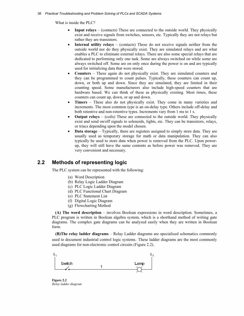
(B)The relay ladder diagrams – Relay Ladder diagrams are specialized schematics commonly used to document industrial control logic systems. These ladder diagrams are the most commonly used diagrams for non-electronic control circuits (Figure 2.2).

Figure 2.2 Relay ladder diagram


37

The “L1” and “L2” designations refer to the two poles of a 120 V AC supply, unless otherwise noted. L1 is the “hot” conductor, and L2 is the grounded (“neutral”) conductor. The symbols used in ladder diagrams are mostly electrical symbols.

The relay logic program can be useful if you create your own programs, modify programs, or if you doubt the validity of the program you have. The relay logic for a process control is represented by ladder diagram and sequence listings. The ladder diagram can be further classified as control ladder diagram and power ladder diagram.

(C) The PLC ladder diagram A ladder diagram is one of the simplest methods used to program a PLC (Figure 2.3).

• It is a graphical programming language evolved from electrical relay circuits. • Each program statement is represented with a line, called the rung that has all

relevant inputs to the left and the output to the right. • The output device of a rung is energized if electric power can conceptually flow from

the left side of the rung to the right side. Input devices are assumed to block the flow of power if they are not activated.

• During the execution of a ladder diagram, the PLC reads the states of all inputs, then determines the states of all outputs starting from the rung at the top side, going down to the last rung, and finally updates the state of the output devices.

Figure 2.3 PLC ladder diagram

(D) PLC function chart The function chart (FCH) may be used for both simple scanning programs and for the

representation of sequence programs (SFC). The logic elements are shown by a basic rectangular symbol and a function designation; negated inputs are indicated by a circle in front of the basic symbol (Figure 2.4).

Figure 2.4 PLC functional chart

Sequential function charts (SFCs) have long been established as a means of designing and implementing sequential control systems utilizing the programmable controllers.

The programming standard IEC 61131-3 includes a graphical implementation of SFCs in its suite of programming languages. Many manufacturers offer programming environments that allow engineers to program controllers using graphical methods to implement the SFCs.


Many systems have sequential operation requirements and SFCs have become a popular method of accurately specifying sequential control requirements. Sequential function charts have many advantages for software development both in the design stage as well as the implementation and testing, maintaining, and fault-finding stages.

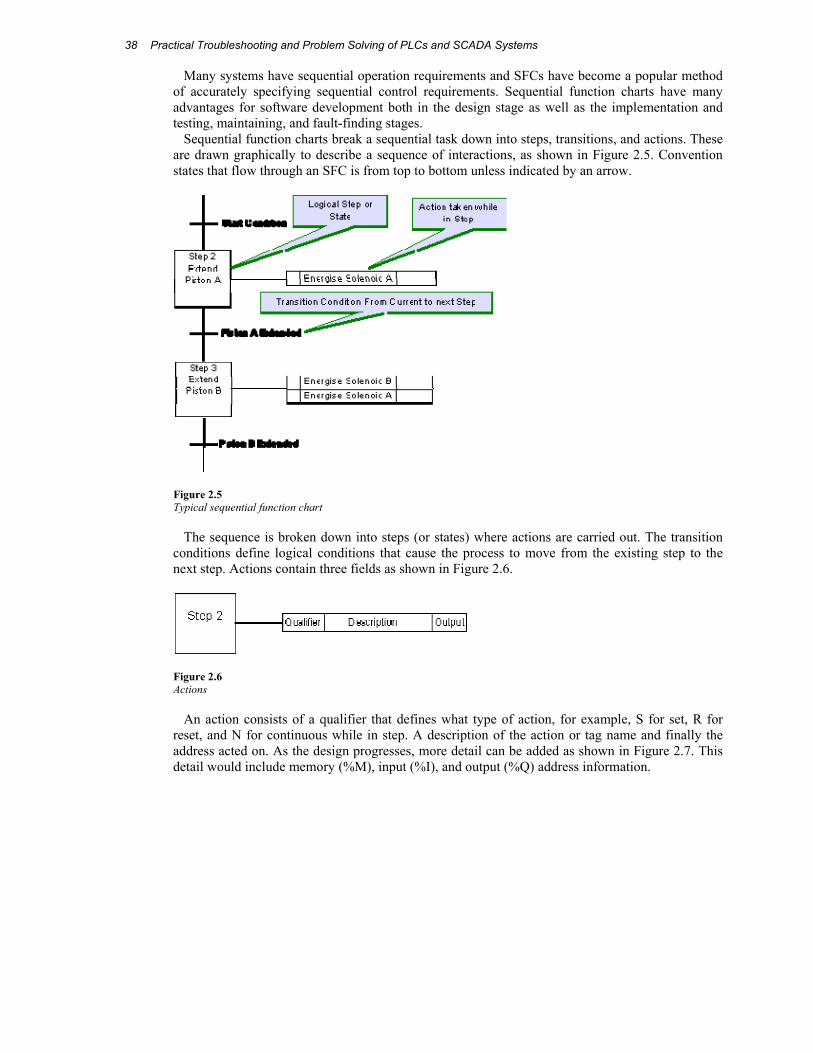
Sequential function charts break a sequential task down into steps, transitions, and actions. These are drawn graphically to describe a sequence of interactions, as shown in Figure 2.5. Convention states that flow through an SFC is from top to bottom unless indicated by an arrow.

Figure 2.5 Typical sequential function chart

The sequence is broken down into steps (or states) where actions are carried out. The transition conditions define logical conditions that cause the process to move from the existing step to the next step. Actions contain three fields as shown in Figure 2.6.

Figure 2.6 Actions

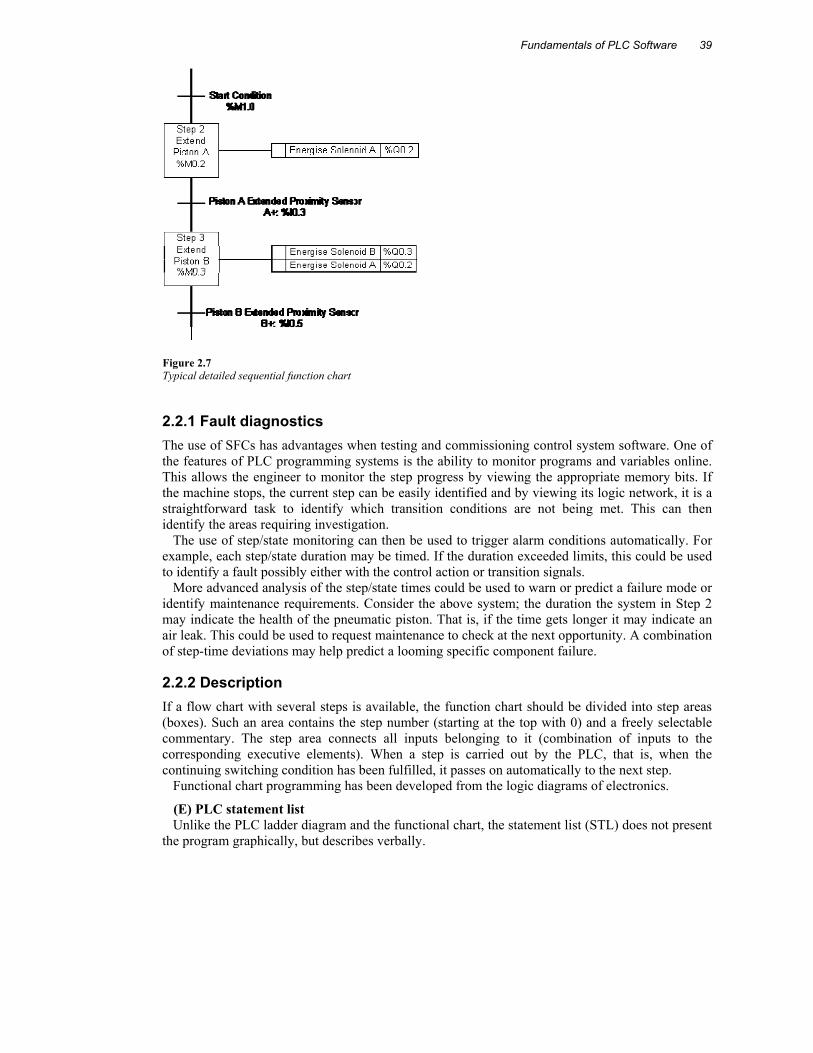
An action consists of a qualifier that defines what type of action, for example, S for set, R for reset, and N for continuous while in step. A description of the action or tag name and finally the address acted on. As the design progresses, more detail can be added as shown in Figure 2.7. This detail would include memory (%M), input (%I), and output (%Q) address information.


39

Figure 2.7 Typical detailed sequential function chart

2.2.1 Fault diagnostics The use of SFCs has advantages when testing and commissioning control system software. One of the features of PLC programming systems is the ability to monitor programs and variables online. This allows the engineer to monitor the step progress by viewing the appropriate memory bits. If the machine stops, the current step can be easily identified and by viewing its logic network, it is a straightforward task to identify which transition conditions are not being met. This can then identify the areas requiring investigation.

The use of step/state monitoring can then be used to trigger alarm conditions automatically. For example, each step/state duration may be timed. If the duration exceeded limits, this could be used to identify a fault possibly either with the control action or transition signals.

More advanced analysis of the step/state times could be used to warn or predict a failure mode or identify maintenance requirements. Consider the above system; the duration the system in Step 2 may indicate the health of the pneumatic piston. That is, if the time gets longer it may indicate an air leak. This could be used to request maintenance to check at the next opportunity. A combination of step-time deviations may help predict a looming specific component failure.

2.2.2 Description If a flow chart with several steps is available, the function chart should be divided into step areas (boxes). Such an area contains the step number (starting at the top with 0) and a freely selectable commentary. The step area connects all inputs belonging to it (combination of inputs to the corresponding executive elements). When a step is carried out by the PLC, that is, when the continuing switching condition has been fulfilled, it passes on automatically to the next step.

Functional chart programming has been developed from the logic diagrams of electronics.

(E) PLC statement list Unlike the PLC ladder diagram and the functional chart, the statement list (STL) does not present

the program graphically, but describes verbally.


The statement list is made up of individual instruction lines. It is possible to write a comment to the right of each instruction line, giving a more precise description of the switching elements. The instruction lines in the statement list are numbered consecutively. The set of instructions (statement) comprises various conditional and executive instructions.

STL program (DIN) L 11 A N 12 = O6 L 13 O 14 = O7 The instructions (Commands) listed in abbreviated form are as follows: L = Load (start of an instruction) A = AND logic element O = OR logic element N = NOT logic element = Set otherwise reset Example: Statement List (Sequence Program)

(F) Digital logic diagram There are many kinds of gates used to implement logical functions. All of them can be

constructed from just three kinds: the AND Gate, the OR Gate, and the NOT Gate.

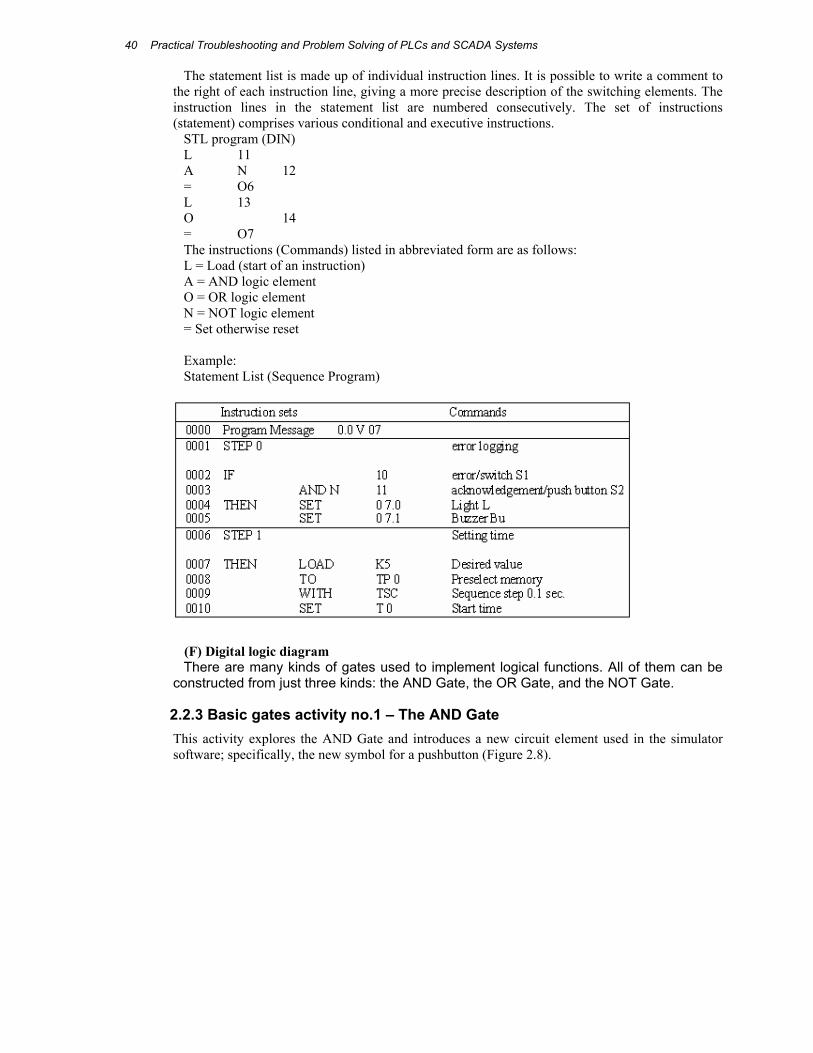
2.2.3 Basic gates activity no.1 – The AND Gate This activity explores the AND Gate and introduces a new circuit element used in the simulator software; specifically, the new symbol for a pushbutton (Figure 2.8).


41

AND Gate menu button AND Gate along with an output LED and two pushbutton inputs

Figure 2.8 AND Gate

A function involving two inputs in which both inputs must be “TRUE” to yield a “TRUE” output, otherwise the output is “FALSE.”

When speaking of gates, we generally refer to the inputs as A and B and the output as Y.

Two symbols for pushbuttons serve as inputs instead of switches (Figure 2.9).

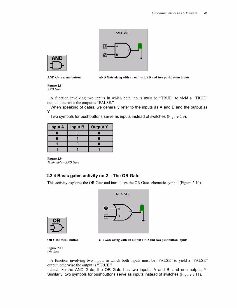
Figure 2.9 Truth table – AND Gate

2.2.4 Basic gates activity no.2 – The OR Gate This activity explores the OR Gate and introduces the OR Gate schematic symbol (Figure 2.10).

OR Gate menu button OR Gate along with an output LED and two pushbutton inputs

Figure 2.10 OR Gate

A function involving two inputs in which both inputs must be “FALSE” to yield a “FALSE” output, otherwise the output is “TRUE.”

Just like the AND Gate, the OR Gate has two inputs, A and B, and one output, Y. Similarly, two symbols for pushbuttons serve as inputs instead of switches (Figure 2.11).


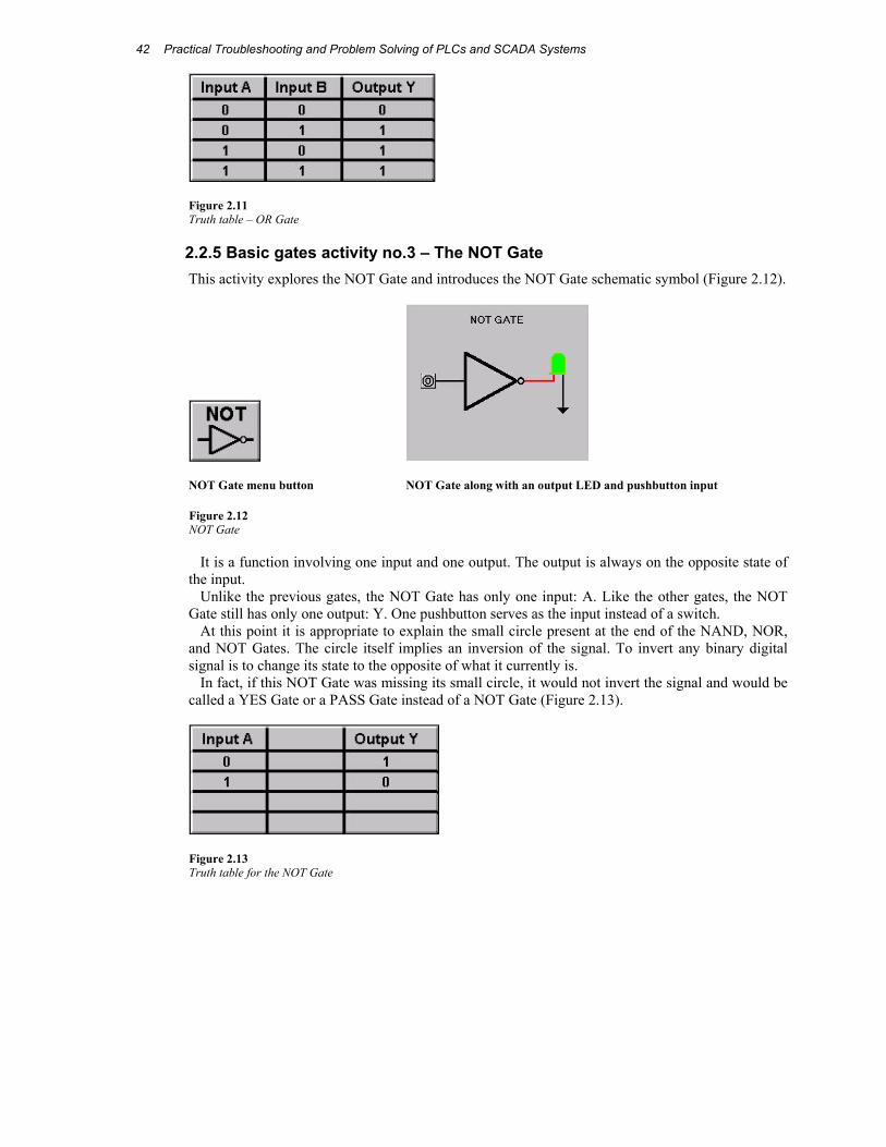
Figure 2.11 Truth table – OR Gate

2.2.5 Basic gates activity no.3 – The NOT Gate This activity explores the NOT Gate and introduces the NOT Gate schematic symbol (Figure 2.12).

NOT Gate menu button NOT Gate along with an output LED and pushbutton input

Figure 2.12 NOT Gate

It is a function involving one input and one output. The output is always on the opposite state of the input.

Unlike the previous gates, the NOT Gate has only one input: A. Like the other gates, the NOT Gate still has only one output: Y. One pushbutton serves as the input instead of a switch.

At this point it is appropriate to explain the small circle present at the end of the NAND, NOR, and NOT Gates. The circle itself implies an inversion of the signal. To invert any binary digital signal is to change its state to the opposite of what it currently is.

In fact, if this NOT Gate was missing its small circle, it would not invert the signal and would be called a YES Gate or a PASS Gate instead of a NOT Gate (Figure 2.13).

Figure 2.13 Truth table for the NOT Gate


43

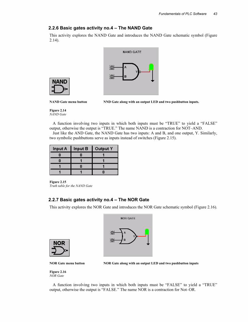
2.2.6 Basic gates activity no.4 – The NAND Gate This activity explores the NAND Gate and introduces the NAND Gate schematic symbol (Figure 2.14).

NAND Gate menu button NND Gate along with an output LED and two pushbutton inputs.

Figure 2.14 NAND Gate

A function involving two inputs in which both inputs must be “TRUE” to yield a “FALSE” output, otherwise the output is “TRUE.” The name NAND is a contraction for NOT–AND.

Just like the AND Gate, the NAND Gate has two inputs: A and B, and one output, Y. Similarly, two symbolic pushbuttons serve as inputs instead of switches (Figure 2.15).

Figure 2.15 Truth table for the NAND Gate

2.2.7 Basic gates activity no.4 – The NOR Gate This activity explores the NOR Gate and introduces the NOR Gate schematic symbol (Figure 2.16).

NOR Gate menu button NOR Gate along with an output LED and two pushbutton inputs

Figure 2.16 NOR Gate

A function involving two inputs in which both inputs must be “FALSE” to yield a “TRUE” output, otherwise the output is “FALSE.” The name NOR is a contraction for Not–OR.


Just like the NAND Gate, the NOR Gate has two inputs, A and B, and one output, Y. Similarly, two symbolic pushbuttons serve as inputs instead of switches (Figure 2.17).

Figure 2.17 Truth table for the NOR Gate

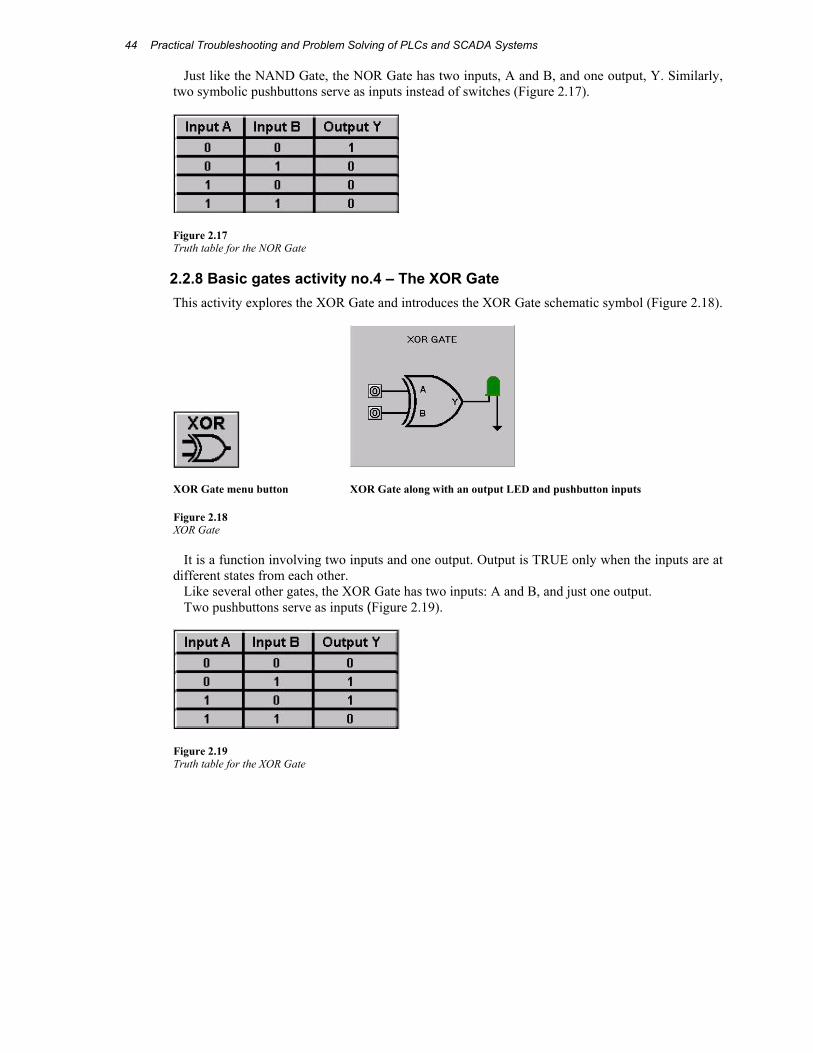
2.2.8 Basic gates activity no.4 – The XOR Gate This activity explores the XOR Gate and introduces the XOR Gate schematic symbol (Figure 2.18).

XOR Gate menu button XOR Gate along with an output LED and pushbutton inputs

Figure 2.18 XOR Gate

It is a function involving two inputs and one output. Output is TRUE only when the inputs are at different states from each other.

Like several other gates, the XOR Gate has two inputs: A and B, and just one output. Two pushbuttons serve as inputs (Figure 2.19).

Figure 2.19 Truth table for the XOR Gate


45

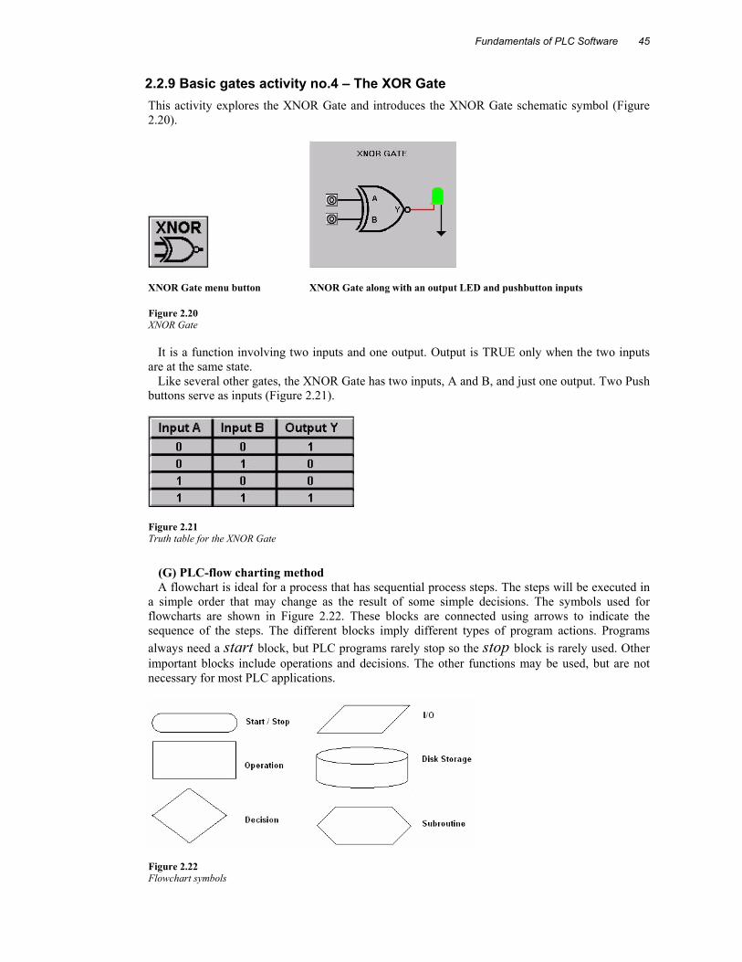
2.2.9 Basic gates activity no.4 – The XOR Gate This activity explores the XNOR Gate and introduces the XNOR Gate schematic symbol (Figure 2.20).

XNOR Gate menu button XNOR Gate along with an output LED and pushbutton inputs

Figure 2.20 XNOR Gate

It is a function involving two inputs and one output. Output is TRUE only when the two inputs are at the same state.

Like several other gates, the XNOR Gate has two inputs, A and B, and just one output. Two Push buttons serve as inputs (Figure 2.21).

Figure 2.21 Truth table for the XNOR Gate

(G) PLC-flow charting method A flowchart is ideal for a process that has sequential process steps. The steps will be executed in

a simple order that may change as the result of some simple decisions. The symbols used for flowcharts are shown in Figure 2.22. These blocks are connected using arrows to indicate the sequence of the steps. The different blocks imply different types of program actions. Programs always need a start block, but PLC programs rarely stop so the stop block is rarely used. Other important blocks include operations and decisions. The other functions may be used, but are not necessary for most PLC applications.

Figure 2.22 Flowchart symbols


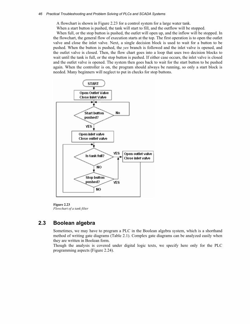
A flowchart is shown in Figure 2.23 for a control system for a large water tank. When a start button is pushed, the tank will start to fill, and the outflow will be stopped. When full, or the stop button is pushed, the outlet will open up, and the inflow will be stopped. In

the flowchart, the general flow of execution starts at the top. The first operation is to open the outlet valve and close the inlet valve. Next, a single decision block is used to wait for a button to be pushed. When the button is pushed, the yes branch is followed and the inlet valve is opened, and the outlet valve is closed. Then, the flow chart goes into a loop that uses two decision blocks to wait until the tank is full, or the stop button is pushed. If either case occurs, the inlet valve is closed and the outlet valve is opened. The system then goes back to wait for the start button to be pushed again. When the controller is on, the program should always be running, so only a start block is needed. Many beginners will neglect to put in checks for stop buttons.

Figure 2.23 Flowchart of a tank filter

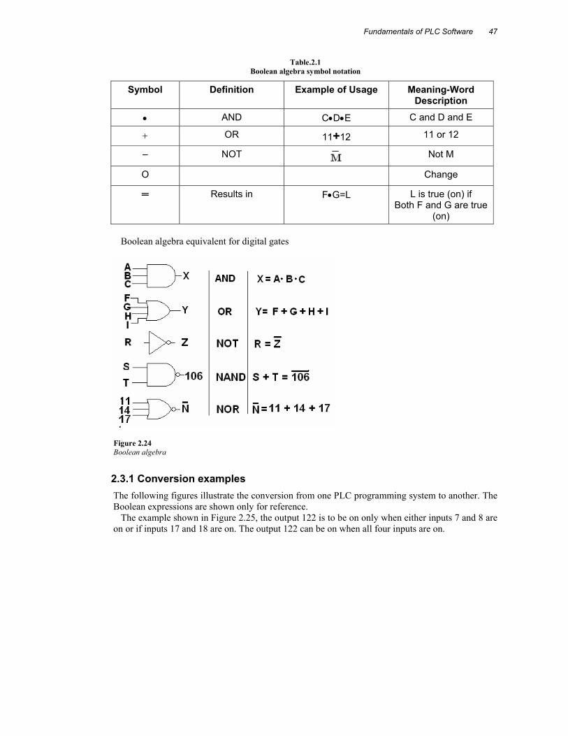
2.3 Boolean algebra Sometimes, we may have to program a PLC in the Boolean algebra system, which is a shorthand method of writing gate diagrams (Table 2.1). Complex gate diagrams can be analyzed easily when they are written in Boolean form. Though the analysis is covered under digital logic texts, we specify here only for the PLC programming aspects (Figure 2.24).


47

Table.2.1 Boolean algebra symbol notation

Symbol Definition Example of Usage Meaning-Word Description

• AND C•D•E C and D and E

+ OR 11+12 11 or 12

– NOT Not M

O Change

═ Results in F•G=L L is true (on) if Both F and G are true

(on) Boolean algebra equivalent for digital gates

Figure 2.24 Boolean algebra

2.3.1 Conversion examples The following figures illustrate the conversion from one PLC programming system to another. The Boolean expressions are shown only for reference.

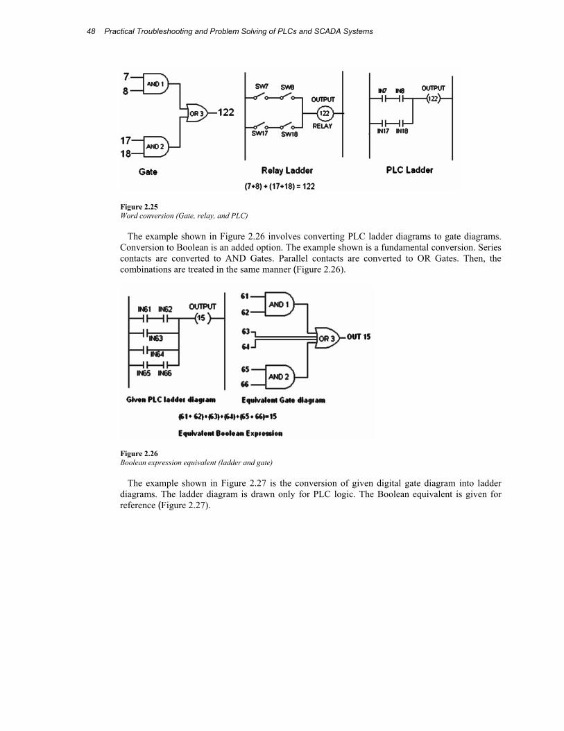
The example shown in Figure 2.25, the output 122 is to be on only when either inputs 7 and 8 are on or if inputs 17 and 18 are on. The output 122 can be on when all four inputs are on.


Figure 2.25 Word conversion (Gate, relay, and PLC)

The example shown in Figure 2.26 involves converting PLC ladder diagrams to gate diagrams. Conversion to Boolean is an added option. The example shown is a fundamental conversion. Series contacts are converted to AND Gates. Parallel contacts are converted to OR Gates. Then, the combinations are treated in the same manner (Figure 2.26).

Figure 2.26 Boolean expression equivalent (ladder and gate)

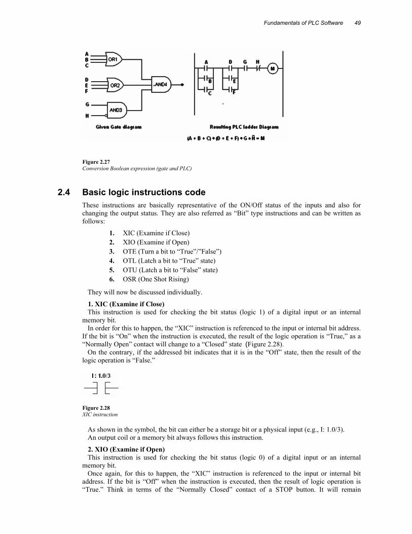
The example shown in Figure 2.27 is the conversion of given digital gate diagram into ladder diagrams. The ladder diagram is drawn only for PLC logic. The Boolean equivalent is given for reference (Figure 2.27).


49

Figure 2.27 Conversion Boolean expression (gate and PLC)

2.4 Basic logic instructions code These instructions are basically representative of the ON/Off status of the inputs and also for changing the output status. They are also referred as “Bit” type instructions and can be written as follows:

1. XIC (Examine if Close) 2. XIO (Examine if Open) 3. OTE (Turn a bit to “True”/”False”) 4. OTL (Latch a bit to “True” state) 5. OTU (Latch a bit to “False” state) 6. OSR (One Shot Rising)

They will now be discussed individually.

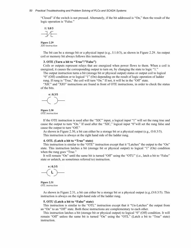
1. XIC (Examine if Close) This instruction is used for checking the bit status (logic 1) of a digital input or an internal

memory bit. In order for this to happen, the “XIC” instruction is referenced to the input or internal bit address.

If the bit is “On” when the instruction is executed, the result of the logic operation is “True,” as a “Normally Open” contact will change to a “Closed” state (Figure 2.28).

On the contrary, if the addressed bit indicates that it is in the “Off” state, then the result of the logic operation is “False.”

Figure 2.28 XIC instruction

As shown in the symbol, the bit can either be a storage bit or a physical input (e.g., I: 1.0/3). An output coil or a memory bit always follows this instruction.

2. XIO (Examine if Open) This instruction is used for checking the bit status (logic 0) of a digital input or an internal

memory bit. Once again, for this to happen, the “XIC” instruction is referenced to the input or internal bit

address. If the bit is “Off” when the instruction is executed, then the result of logic operation is “True.” Think in terms of the “Normally Closed” contact of a STOP button. It will remain


“Closed” if the switch is not pressed. Alternately, if the bit addressed is “On,” then the result of the logic operation is “False.”

Figure 2.29 XIO instruction

The bit can be a storage bit or a physical input (e.g., I:1.0/3), as shown in Figure 2.29. An output coil or memory bit always follows this instruction.

3. OTE (Turn a bit to “True”/”False”) Coils or outputs represent relays that are energized when power flows to them. When a coil is

energized, it causes the corresponding output to turn on, by changing the state to logic “1.” The output instruction turns a bit (storage bit or physical output) status or output coil to logical “0” (Off) condition or to logical “1” (On) depending on the result of logic operation of ladder rung. If rung is “True,” the coil will turn “On.” If not, it will be in the “Off” state. “XIC” and “XIO” instructions are found in front of OTE instructions, in order to check the status

of the bits.

Figure 2.30 OTE instruction

If the OTE instruction is used after the “XIC” input, a logical input “1” will set the rung true and cause the output to turn “On.” If used after the “XIC,” logical input “0”will set the rung false and cause the output to turn “Off.”

As shown in Figure 2.30, a bit can either be a storage bit or a physical output (e.g., O:0.3/5). This instruction is always at the right hand side of the ladder rung.

4. OTL (Latch a bit to “True” state) This instruction is similar to the “OTE” instruction except that it “Latches” the output to the “On”

state. This instruction latches a bit (storage bit or physical output) to logical “1” (On) condition when the rung goes “True.”

It will remain “On” until the same bit is turned “Off” using the “OTU” (i.e., latch a bit to “False” state or unlatch, as sometimes referred to) instruction.

Figure 2.31 OTL instruction

As shown in Figure 2.31, a bit can either be a storage bit or a physical output (e.g.,O:0.3/5). This instruction is always on the right-hand side of the ladder rung.

5. OTU (Latch a bit to “False” state) This instruction is similar to the “OTL” instruction except that it “Un-Latches” the output from

an “On” to an “Off” state. Both these instructions are complementary to each other. This instruction latches a bit (storage bit or physical output) to logical “0” (Off) condition. It will

remain “Off” unless the same bit is turned “On” using the “OTL” (Latch a bit to “True” state) instruction.


51

Figure 2.32 OTU instruction

As shown in the Figure 2.32, a bit can either be a storage bit or a physical output (e.g., O:0.3/5). This instruction is found at the right-hand side of the ladder rung.

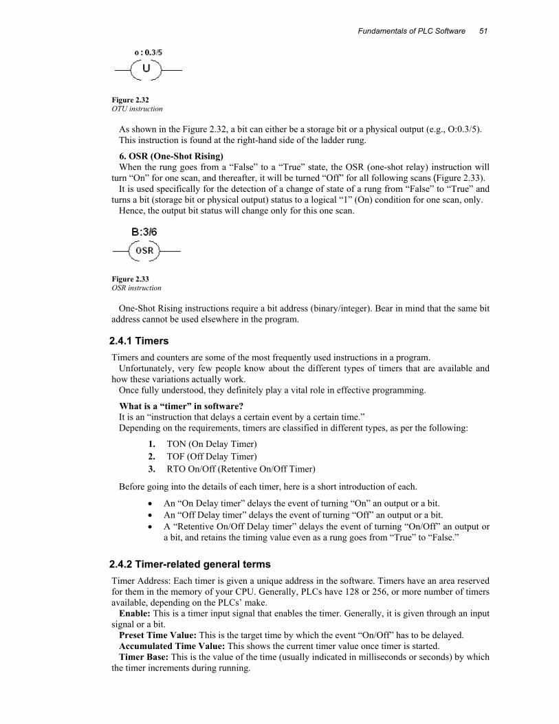
6. OSR (One-Shot Rising) When the rung goes from a “False” to a “True” state, the OSR (one-shot relay) instruction will

turn “On” for one scan, and thereafter, it will be turned “Off” for all following scans (Figure 2.33). It is used specifically for the detection of a change of state of a rung from “False” to “True” and

turns a bit (storage bit or physical output) status to a logical “1” (On) condition for one scan, only. Hence, the output bit status will change only for this one scan.

Figure 2.33 OSR instruction

One-Shot Rising instructions require a bit address (binary/integer). Bear in mind that the same bit address cannot be used elsewhere in the program.

2.4.1 Timers Timers and counters are some of the most frequently used instructions in a program.

Unfortunately, very few people know about the different types of timers that are available and how these variations actually work.

Once fully understood, they definitely play a vital role in effective programming.

What is a “timer” in software? It is an “instruction that delays a certain event by a certain time.” Depending on the requirements, timers are classified in different types, as per the following:

1. TON (On Delay Timer) 2. TOF (Off Delay Timer) 3. RTO On/Off (Retentive On/Off Timer)

Before going into the details of each timer, here is a short introduction of each.

• An “On Delay timer” delays the event of turning “On” an output or a bit. • An “Off Delay timer” delays the event of turning “Off” an output or a bit. • A “Retentive On/Off Delay timer” delays the event of turning “On/Off” an output or

a bit, and retains the timing value even as a rung goes from “True” to “False.”

2.4.2 Timer-related general terms Timer Address: Each timer is given a unique address in the software. Timers have an area reserved for them in the memory of your CPU. Generally, PLCs have 128 or 256, or more number of timers available, depending on the PLCs’ make.

Enable: This is a timer input signal that enables the timer. Generally, it is given through an input signal or a bit.

Preset Time Value: This is the target time by which the event “On/Off” has to be delayed. Accumulated Time Value: This shows the current timer value once timer is started. Timer Base: This is the value of the time (usually indicated in milliseconds or seconds) by which

the timer increments during running.


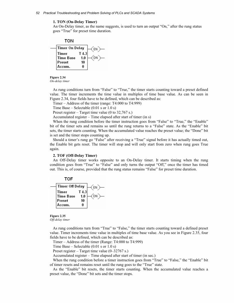
1. TON (On-Delay Timer) An On-Delay timer, as the name suggests, is used to turn an output “On,” after the rung status goes “True” for preset time duration.

Figure 2.34 On-delay timer

As rung conditions turn from “False” to “True,” the timer starts counting toward a preset defined value. The timer increments the time value in multiples of time base value. As can be seen in Figure 2.34, four fields have to be defined, which can be described as:

Timer – Address of the timer (range: T4:000 to T4:999) Time Base – Selectable (0.01 s or 1.0 s) Preset register – Target time value (0 to 32,767 s.) Accumulated register – Time elapsed after start of timer (in s) When the rung condition before the timer instruction goes from “False” to “True,” the “Enable”

bit of the timer sets and remains so until the rung returns to a “False” state. As the “Enable” bit sets, the timer starts counting. When the accumulated value reaches the preset value; the “Done” bit is set and the timer stops counting up.

Should a timer’s rung go “False” after receiving a “True” signal before it has actually timed out, the Enable bit gets reset. The timer will stop and will only start from zero when rung goes True again.

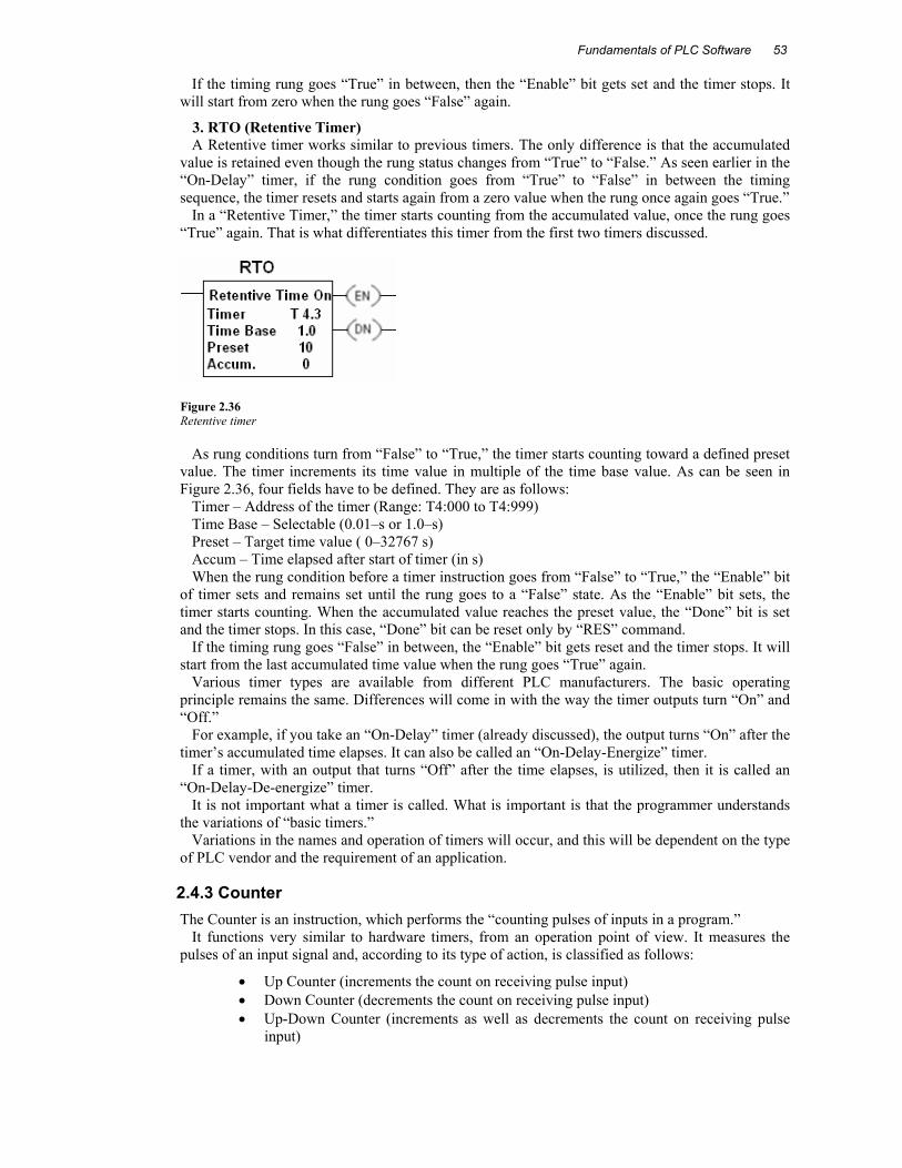
2. TOF (Off-Delay Timer) An Off-Delay timer works opposite to an On-Delay timer. It starts timing when the rung

condition goes from “True” to “False” and only turns the output “Off,” once the timer has timed out. This is, of course, provided that the rung status remains “False” for preset time duration.

Figure 2.35 Off-delay timer

As rung conditions turn from “True” to “False,” the timer starts counting toward a defined preset value. Timer increments time value in multiples of time base value. As you see in Figure 2.35, four fields have to be defined, which can be described as:

Timer – Address of the timer (Range: T4:000 to T4:999) Time Base – Selectable (0.01 s or 1.0 s) Preset register – Target time value (0–32767 s.) Accumulated register – Time elapsed after start of timer (in sec.) When the rung condition before a timer instruction goes from “True” to “False,” the “Enable” bit

of timer resets and remains reset until the rung goes to the “True” state. As the “Enable” bit resets, the timer starts counting. When the accumulated value reaches a

preset value, the “Done” bit sets and the timer stops.


53

If the timing rung goes “True” in between, then the “Enable” bit gets set and the timer stops. It will start from zero when the rung goes “False” again.

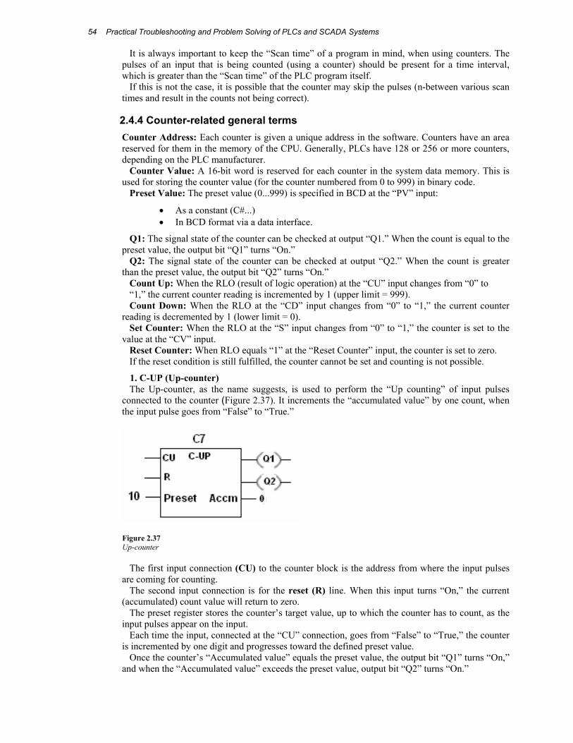
3. RTO (Retentive Timer) A Retentive timer works similar to previous timers. The only difference is that the accumulated

value is retained even though the rung status changes from “True” to “False.” As seen earlier in the “On-Delay” timer, if the rung condition goes from “True” to “False” in between the timing sequence, the timer resets and starts again from a zero value when the rung once again goes “True.”

In a “Retentive Timer,” the timer starts counting from the accumulated value, once the rung goes “True” again. That is what differentiates this timer from the first two timers discussed.

Figure 2.36 Retentive timer

As rung conditions turn from “False” to “True,” the timer starts counting toward a defined preset value. The timer increments its time value in multiple of the time base value. As can be seen in Figure 2.36, four fields have to be defined. They are as follows:

Timer – Address of the timer (Range: T4:000 to T4:999) Time Base – Selectable (0.01–s or 1.0–s) Preset – Target time value ( 0–32767 s) Accum – Time elapsed after start of timer (in s) When the rung condition before a timer instruction goes from “False” to “True,” the “Enable” bit

of timer sets and remains set until the rung goes to a “False” state. As the “Enable” bit sets, the timer starts counting. When the accumulated value reaches the preset value, the “Done” bit is set and the timer stops. In this case, “Done” bit can be reset only by “RES” command.

If the timing rung goes “False” in between, the “Enable” bit gets reset and the timer stops. It will start from the last accumulated time value when the rung goes “True” again.

Various timer types are available from different PLC manufacturers. The basic operating principle remains the same. Differences will come in with the way the timer outputs turn “On” and “Off.”

For example, if you take an “On-Delay” timer (already discussed), the output turns “On” after the timer’s accumulated time elapses. It can also be called an “On-Delay-Energize” timer.

If a timer, with an output that turns “Off” after the time elapses, is utilized, then it is called an “On-Delay-De-energize” timer.

It is not important what a timer is called. What is important is that the programmer understands the variations of “basic timers.”

Variations in the names and operation of timers will occur, and this will be dependent on the type of PLC vendor and the requirement of an application.

2.4.3 Counter The Counter is an instruction, which performs the “counting pulses of inputs in a program.”

It functions very similar to hardware timers, from an operation point of view. It measures the pulses of an input signal and, according to its type of action, is classified as follows:

• Up Counter (increments the count on receiving pulse input) • Down Counter (decrements the count on receiving pulse input) • Up-Down Counter (increments as well as decrements the count on receiving pulse

input)


It is always important to keep the “Scan time” of a program in mind, when using counters. The pulses of an input that is being counted (using a counter) should be present for a time interval, which is greater than the “Scan time” of the PLC program itself.

If this is not the case, it is possible that the counter may skip the pulses (n-between various scan times and result in the counts not being correct).

2.4.4 Counter-related general terms Counter Address: Each counter is given a unique address in the software. Counters have an area reserved for them in the memory of the CPU. Generally, PLCs have 128 or 256 or more counters, depending on the PLC manufacturer.

Counter Value: A 16-bit word is reserved for each counter in the system data memory. This is used for storing the counter value (for the counter numbered from 0 to 999) in binary code.

Preset Value: The preset value (0...999) is specified in BCD at the “PV” input:

• As a constant (C#...) • In BCD format via a data interface.

Q1: The signal state of the counter can be checked at output “Q1.” When the count is equal to the preset value, the output bit “Q1” turns “On.”

Q2: The signal state of the counter can be checked at output “Q2.” When the count is greater than the preset value, the output bit “Q2” turns “On.”

Count Up: When the RLO (result of logic operation) at the “CU” input changes from “0” to “1,” the current counter reading is incremented by 1 (upper limit = 999). Count Down: When the RLO at the “CD” input changes from “0” to “1,” the current counter

reading is decremented by 1 (lower limit = 0). Set Counter: When the RLO at the “S” input changes from “0” to “1,” the counter is set to the

value at the “CV” input. Reset Counter: When RLO equals “1” at the “Reset Counter” input, the counter is set to zero. If the reset condition is still fulfilled, the counter cannot be set and counting is not possible.

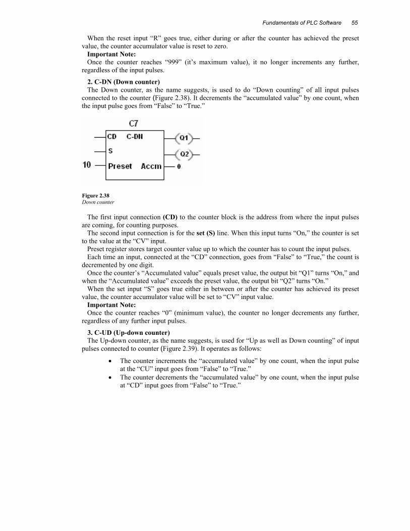
1. C-UP (Up-counter) The Up-counter, as the name suggests, is used to perform the “Up counting” of input pulses

connected to the counter (Figure 2.37). It increments the “accumulated value” by one count, when the input pulse goes from “False” to “True.”

Figure 2.37 Up-counter

The first input connection (CU) to the counter block is the address from where the input pulses are coming for counting.

The second input connection is for the reset (R) line. When this input turns “On,” the current (accumulated) count value will return to zero.

The preset register stores the counter’s target value, up to which the counter has to count, as the input pulses appear on the input.

Each time the input, connected at the “CU” connection, goes from “False” to “True,” the counter is incremented by one digit and progresses toward the defined preset value.

Once the counter’s “Accumulated value” equals the preset value, the output bit “Q1” turns “On,” and when the “Accumulated value” exceeds the preset value, output bit “Q2” turns “On.”


55

When the reset input “R” goes true, either during or after the counter has achieved the preset value, the counter accumulator value is reset to zero.

Important Note: Once the counter reaches “999” (it’s maximum value), it no longer increments any further,

regardless of the input pulses.

2. C-DN (Down counter) The Down counter, as the name suggests, is used to do “Down counting” of all input pulses

connected to the counter (Figure 2.38). It decrements the “accumulated value” by one count, when the input pulse goes from “False” to “True.”

Figure 2.38 Down counter

The first input connection (CD) to the counter block is the address from where the input pulses are coming, for counting purposes.

The second input connection is for the set (S) line. When this input turns “On,” the counter is set to the value at the “CV” input.

Preset register stores target counter value up to which the counter has to count the input pulses. Each time an input, connected at the “CD” connection, goes from “False” to “True,” the count is

decremented by one digit. Once the counter’s “Accumulated value” equals preset value, the output bit “Q1” turns “On,” and

when the “Accumulated value” exceeds the preset value, the output bit “Q2” turns “On.” When the set input “S” goes true either in between or after the counter has achieved its preset

value, the counter accumulator value will be set to “CV” input value. Important Note: Once the counter reaches “0” (minimum value), the counter no longer decrements any further,

regardless of any further input pulses.

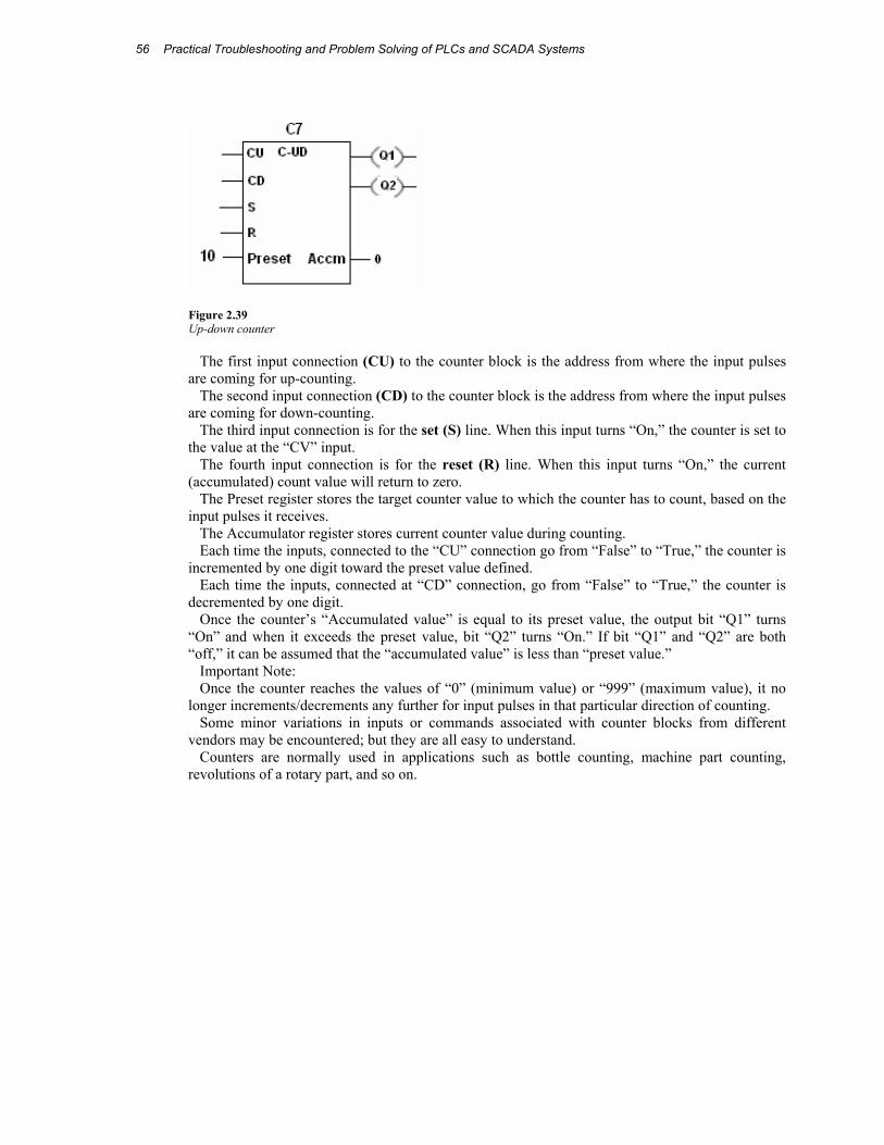
3. C-UD (Up-down counter) The Up-down counter, as the name suggests, is used for “Up as well as Down counting” of input

pulses connected to counter (Figure 2.39). It operates as follows:

• The counter increments the “accumulated value” by one count, when the input pulse at the “CU” input goes from “False” to “True.”

• The counter decrements the “accumulated value” by one count, when the input pulse at “CD” input goes from “False” to “True.”


Figure 2.39 Up-down counter

The first input connection (CU) to the counter block is the address from where the input pulses are coming for up-counting.

The second input connection (CD) to the counter block is the address from where the input pulses are coming for down-counting.

The third input connection is for the set (S) line. When this input turns “On,” the counter is set to the value at the “CV” input.

The fourth input connection is for the reset (R) line. When this input turns “On,” the current (accumulated) count value will return to zero.

The Preset register stores the target counter value to which the counter has to count, based on the input pulses it receives.

The Accumulator register stores current counter value during counting. Each time the inputs, connected to the “CU” connection go from “False” to “True,” the counter is

incremented by one digit toward the preset value defined. Each time the inputs, connected at “CD” connection, go from “False” to “True,” the counter is

decremented by one digit. Once the counter’s “Accumulated value” is equal to its preset value, the output bit “Q1” turns

“On” and when it exceeds the preset value, bit “Q2” turns “On.” If bit “Q1” and “Q2” are both “off,” it can be assumed that the “accumulated value” is less than “preset value.”

Important Note: Once the counter reaches the values of “0” (minimum value) or “999” (maximum value), it no

longer increments/decrements any further for input pulses in that particular direction of counting. Some minor variations in inputs or commands associated with counter blocks from different

vendors may be encountered; but they are all easy to understand. Counters are normally used in applications such as bottle counting, machine part counting,

revolutions of a rotary part, and so on.


57

2.5 Graphical representation-functional logic diagram

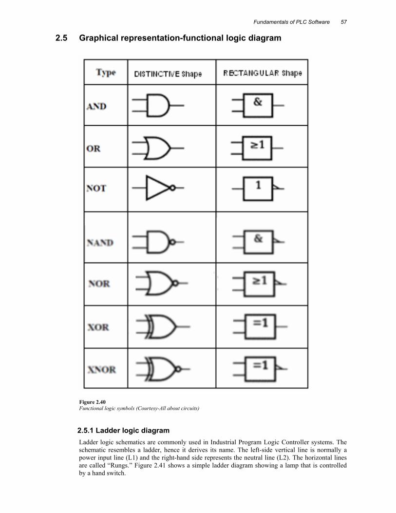
Figure 2.40 Functional logic symbols (Courtesy-All about circuits)

2.5.1 Ladder logic diagram Ladder logic schematics are commonly used in Industrial Program Logic Controller systems. The schematic resembles a ladder, hence it derives its name. The left-side vertical line is normally a power input line (L1) and the right-hand side represents the neutral line (L2). The horizontal lines are called “Rungs.” Figure 2.41 shows a simple ladder diagram showing a lamp that is controlled by a hand switch.


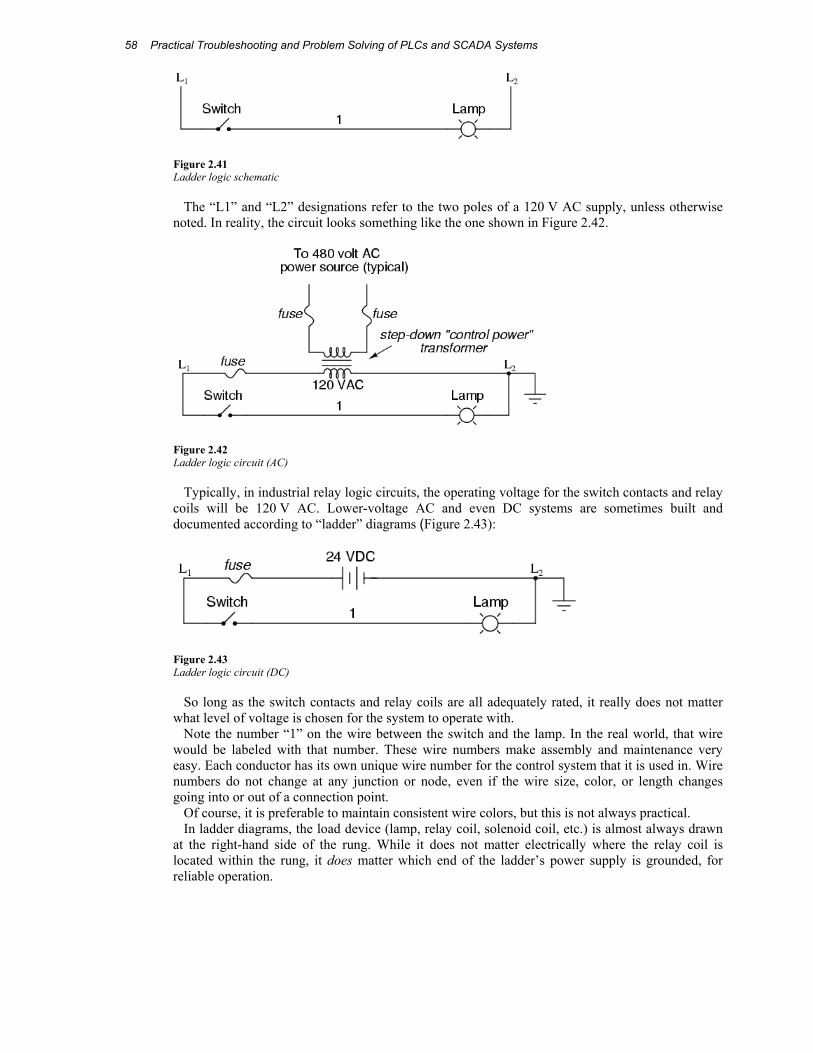
Figure 2.41 Ladder logic schematic

The “L1” and “L2” designations refer to the two poles of a 120 V AC supply, unless otherwise noted. In reality, the circuit looks something like the one shown in Figure 2.42.

Figure 2.42 Ladder logic circuit (AC)

Typically, in industrial relay logic circuits, the operating voltage for the switch contacts and relay coils will be 120 V AC. Lower-voltage AC and even DC systems are sometimes built and documented according to “ladder” diagrams (Figure 2.43):

Figure 2.43 Ladder logic circuit (DC)

So long as the switch contacts and relay coils are all adequately rated, it really does not matter what level of voltage is chosen for the system to operate with.

Note the number “1” on the wire between the switch and the lamp. In the real world, that wire would be labeled with that number. These wire numbers make assembly and maintenance very easy. Each conductor has its own unique wire number for the control system that it is used in. Wire numbers do not change at any junction or node, even if the wire size, color, or length changes going into or out of a connection point.

Of course, it is preferable to maintain consistent wire colors, but this is not always practical. In ladder diagrams, the load device (lamp, relay coil, solenoid coil, etc.) is almost always drawn

at the right-hand side of the rung. While it does not matter electrically where the relay coil is located within the rung, it does matter which end of the ladder’s power supply is grounded, for reliable operation.


59

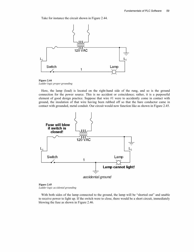
Take for instance the circuit shown in Figure 2.44.

Figure 2.44 Ladder logic proper grounding

Here, the lamp (load) is located on the right-hand side of the rung, and so is the ground connection for the power source. This is no accident or coincidence; rather, it is a purposeful element of good design practice. Suppose that wire #1 were to accidently come in contact with ground, the insulation of that wire having been rubbed off so that the bare conductor came in contact with grounded, metal conduit. Our circuit would now function like as shown in Figure 2.45.

Figure 2.45 Ladder logic accidental grounding

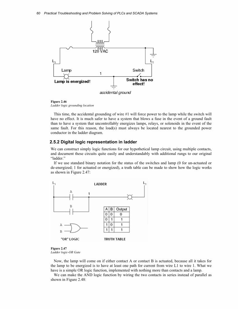
With both sides of the lamp connected to the ground, the lamp will be “shorted out” and unable to receive power to light up. If the switch were to close, there would be a short circuit, immediately blowing the fuse as shown in Figure 2.46.


Figure 2.46 Ladder logic grounding location

This time, the accidental grounding of wire #1 will force power to the lamp while the switch will have no effect. It is much safer to have a system that blows a fuse in the event of a ground fault than to have a system that uncontrollably energizes lamps, relays, or solenoids in the event of the same fault. For this reason, the load(s) must always be located nearest to the grounded power conductor in the ladder diagram.

2.5.2 Digital logic representation in ladder We can construct simply logic functions for our hypothetical lamp circuit, using multiple contacts, and document these circuits quite easily and understandably with additional rungs to our original “ladder.”

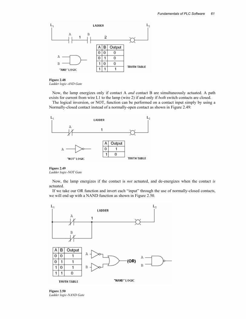
If we use standard binary notation for the status of the switches and lamp (0 for un-actuated or de-energized; 1 for actuated or energized), a truth table can be made to show how the logic works as shown in Figure 2.47:

Figure 2.47 Ladder logic-OR Gate

Now, the lamp will come on if either contact A or contact B is actuated, because all it takes for the lamp to be energized is to have at least one path for current from wire L1 to wire 1. What we have is a simple OR logic function, implemented with nothing more than contacts and a lamp.

We can make the AND logic function by wiring the two contacts in series instead of parallel as shown in Figure 2.48:


61

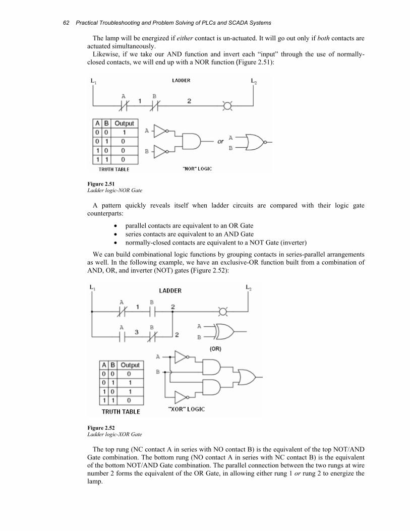
Figure 2.48 Ladder logic-AND Gate

Now, the lamp energizes only if contact A and contact B are simultaneously actuated. A path exists for current from wire L1 to the lamp (wire 2) if and only if both switch contacts are closed.

The logical inversion, or NOT, function can be performed on a contact input simply by using a Normally-closed contact instead of a normally-open contact as shown in Figure 2.49:

Figure 2.49 Ladder logic-NOT Gate

Now, the lamp energizes if the contact is not actuated, and de-energizes when the contact is actuated.

If we take our OR function and invert each “input” through the use of normally-closed contacts, we will end up with a NAND function as shown in Figure 2.50.

Figure 2.50 Ladder logic-NAND Gate


The lamp will be energized if either contact is un-actuated. It will go out only if both contacts are actuated simultaneously.

Likewise, if we take our AND function and invert each “input” through the use of normally-closed contacts, we will end up with a NOR function (Figure 2.51):

Figure 2.51 Ladder logic-NOR Gate

A pattern quickly reveals itself when ladder circuits are compared with their logic gate counterparts:

• parallel contacts are equivalent to an OR Gate • series contacts are equivalent to an AND Gate • normally-closed contacts are equivalent to a NOT Gate (inverter)

We can build combinational logic functions by grouping contacts in series-parallel arrangements as well. In the following example, we have an exclusive-OR function built from a combination of AND, OR, and inverter (NOT) gates (Figure 2.52):

Figure 2.52 Ladder logic-XOR Gate

The top rung (NC contact A in series with NO contact B) is the equivalent of the top NOT/AND Gate combination. The bottom rung (NO contact A in series with NC contact B) is the equivalent of the bottom NOT/AND Gate combination. The parallel connection between the two rungs at wire number 2 forms the equivalent of the OR Gate, in allowing either rung 1 or rung 2 to energize the lamp.


63

To make the exclusive-OR function, we had to use two contacts per input: one for direct input and the other for “inverted” input. The two “A” contacts are physically actuated by the same mechanism, as are the two “B” contacts. The common association between the contacts is denoted by the label of the contact. There is no limit to how many contacts per switch can be represented in a ladder diagram, as each new contact on any switch or relay (either normally-open or normally-closed) used in the diagram is simply marked with the same label.

Sometimes, multiple contacts on a single switch (or relay) are designated by compound labels, such as “A-1” and “A-2” instead of two “A” labels. This may be especially useful if you want to specifically designate which set of contacts on each switch or relay is being used for which part of a circuit. For simplicity’s sake, I’ll refrain from such elaborate labeling in this lesson. If you see a common label for multiple contacts, you know those contacts are all actuated by the same mechanism.

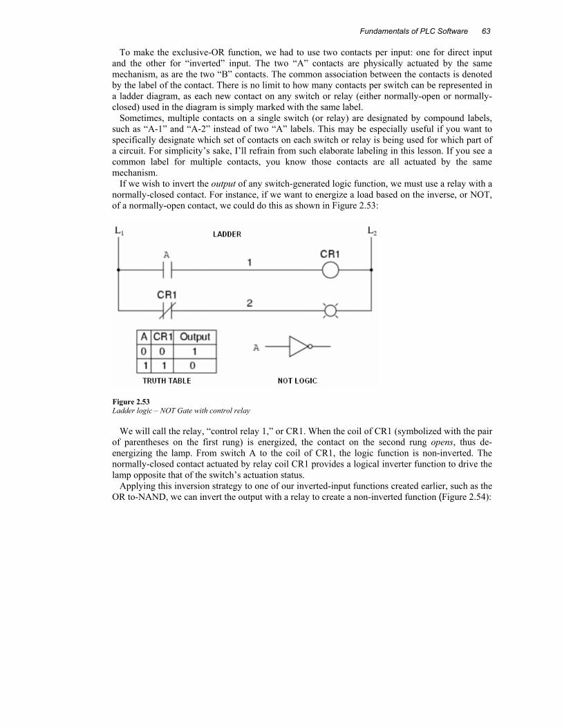
If we wish to invert the output of any switch-generated logic function, we must use a relay with a normally-closed contact. For instance, if we want to energize a load based on the inverse, or NOT, of a normally-open contact, we could do this as shown in Figure 2.53:

Figure 2.53 Ladder logic – NOT Gate with control relay

We will call the relay, “control relay 1,” or CR1. When the coil of CR1 (symbolized with the pair of parentheses on the first rung) is energized, the contact on the second rung opens, thus de-energizing the lamp. From switch A to the coil of CR1, the logic function is non-inverted. The normally-closed contact actuated by relay coil CR1 provides a logical inverter function to drive the lamp opposite that of the switch’s actuation status.

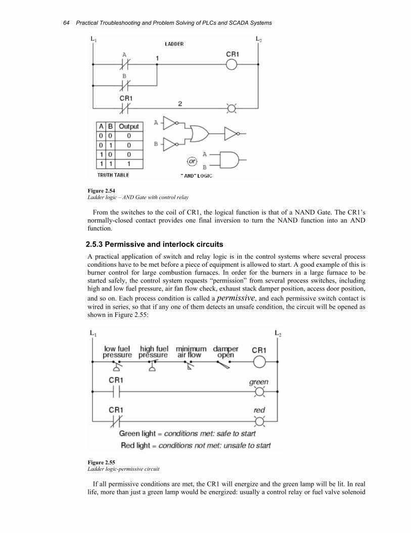
Applying this inversion strategy to one of our inverted-input functions created earlier, such as the OR to-NAND, we can invert the output with a relay to create a non-inverted function (Figure 2.54):


Figure 2.54 Ladder logic – AND Gate with control relay

From the switches to the coil of CR1, the logical function is that of a NAND Gate. The CR1’s normally-closed contact provides one final inversion to turn the NAND function into an AND function.

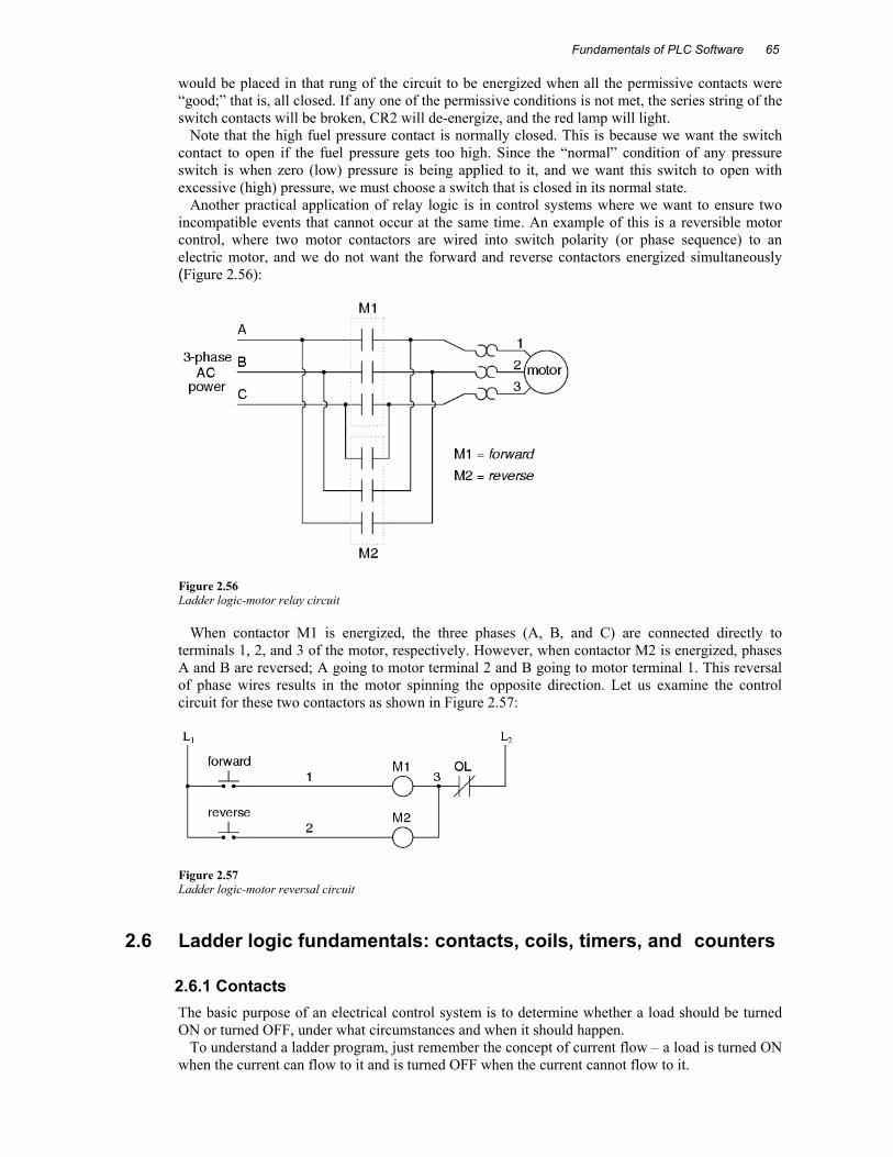
2.5.3 Permissive and interlock circuits A practical application of switch and relay logic is in the control systems where several process conditions have to be met before a piece of equipment is allowed to start. A good example of this is burner control for large combustion furnaces. In order for the burners in a large furnace to be started safely, the control system requests “permission” from several process switches, including high and low fuel pressure, air fan flow check, exhaust stack damper position, access door position, and so on. Each process condition is called a permissive, and each permissive switch contact is wired in series, so that if any one of them detects an unsafe condition, the circuit will be opened as shown in Figure 2.55:

Figure 2.55 Ladder logic-permissive circuit

If all permissive conditions are met, the CR1 will energize and the green lamp will be lit. In real life, more than just a green lamp would be energized: usually a control relay or fuel valve solenoid


65

would be placed in that rung of the circuit to be energized when all the permissive contacts were “good;” that is, all closed. If any one of the permissive conditions is not met, the series string of the switch contacts will be broken, CR2 will de-energize, and the red lamp will light.

Note that the high fuel pressure contact is normally closed. This is because we want the switch contact to open if the fuel pressure gets too high. Since the “normal” condition of any pressure switch is when zero (low) pressure is being applied to it, and we want this switch to open with excessive (high) pressure, we must choose a switch that is closed in its normal state.

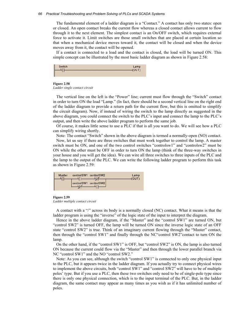
Another practical application of relay logic is in control systems where we want to ensure two incompatible events that cannot occur at the same time. An example of this is a reversible motor control, where two motor contactors are wired into switch polarity (or phase sequence) to an electric motor, and we do not want the forward and reverse contactors energized simultaneously (Figure 2.56):

Figure 2.56 Ladder logic-motor relay circuit

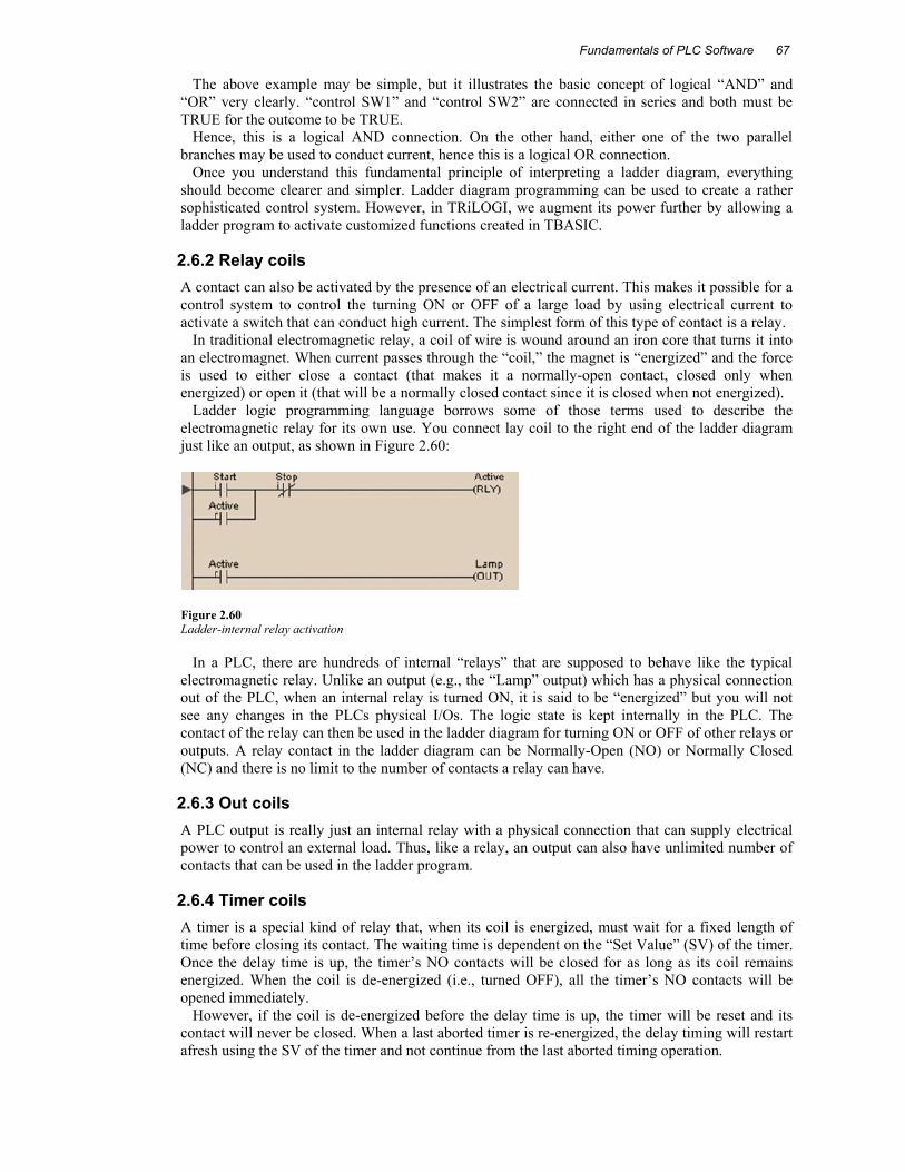
When contactor M1 is energized, the three phases (A, B, and C) are connected directly to terminals 1, 2, and 3 of the motor, respectively. However, when contactor M2 is energized, phases A and B are reversed; A going to motor terminal 2 and B going to motor terminal 1. This reversal of phase wires results in the motor spinning the opposite direction. Let us examine the control circuit for these two contactors as shown in Figure 2.57:

Figure 2.57 Ladder logic-motor reversal circuit

2.6 Ladder logic fundamentals: contacts, coils, timers, and counters

2.6.1 Contacts The basic purpose of an electrical control system is to determine whether a load should be turned ON or turned OFF, under what circumstances and when it should happen.

To understand a ladder program, just remember the concept of current flow – a load is turned ON when the current can flow to it and is turned OFF when the current cannot flow to it.


The fundamental element of a ladder diagram is a “Contact.” A contact has only two states: open or closed. An open contact breaks the current flow whereas a closed contact allows current to flow through it to the next element. The simplest contact is an On/OFF switch, which requires external force to activate it. Limit switches are those small switches that are placed at certain location so that when a mechanical device moves toward it, the contact will be closed and when the device moves away from it, the contact will be opened.

If a contact is connected to a load and the contact is closed, the load will be turned ON. This simple concept can be illustrated by the most basic ladder diagram as shown in Figure 2.58:

Figure 2.58 Ladder single contact circuit

The vertical line on the left is the “Power” line; current must flow through the “Switch” contact in order to turn ON the load “Lamp.” (In fact, there should be a second vertical line on the right end of the ladder diagram to provide a return path for the current flow, but this is omitted to simplify the circuit diagram). Now, if instead of wiring the switch to the lamp directly as suggested in the above diagram, you could connect the switch to the PLC’s input and connect the lamp to the PLC’s output, and then write the above ladder program to perform the same job.

Of course, it makes little sense to use a PLC if that is all you want to do. We will see how a PLC can simplify wiring shortly.

Note: The contact “Switch” shown in the above diagram is termed a normally-open (NO) contact. Now, let us say if there are three switches that must work together to control the lamp. A master

switch must be ON, and one of the two control switches “controlsw1” and “controlsw2” must be ON while the other must be OFF in order to turn ON the lamp (think of the three-way switches in your house and you will get the idea). We can wire all three switches to three inputs of the PLC and the lamp to the output of the PLC. We can write the following ladder program to perform this task as shown in Figure 2.59:

Figure 2.59 Ladder multiple contact circuit

A contact with a “/” across its body is a normally closed (NC) contact. What it means is that the ladder program is using the “inverse” of the logic state of the input to interpret the diagram.

Hence in the above ladder diagram, if the “Master” and the “control SW1” are turned ON, but “control SW2” is turned OFF, the lamp will be turned ON since the inverse logic state of an OFF state “control SW2” is true. Think of an imaginary current flowing through the “Master” contact, then through the “control SW1” and finally through the NC“control SW2”contact to turn ON the lamp.

On the other hand, if the “control SW1” is OFF, but “control SW2” is ON, the lamp is also turned ON because the current could flow via the “Master” and then through the lower parallel branch via NC “control SW1” and the NO “control SW2.”

Note: As you can see, although the switch “control SW1” is connected to only one physical input to the PLC, but it appears twice in the ladder diagram. If you actually try to connect physical wires to implement the above circuits, both “control SW1” and “control SW2” will have to be of multiple poles’ type. But if you use a PLC, then these two switches only need to be of single-pole type since there is only one physical connection, which is to the input terminal of the PLC. But, in the ladder diagram, the same contact may appear as many times as you wish as if it has unlimited number of poles.


67

The above example may be simple, but it illustrates the basic concept of logical “AND” and “OR” very clearly. “control SW1” and “control SW2” are connected in series and both must be TRUE for the outcome to be TRUE.

Hence, this is a logical AND connection. On the other hand, either one of the two parallel branches may be used to conduct current, hence this is a logical OR connection.

Once you understand this fundamental principle of interpreting a ladder diagram, everything should become clearer and simpler. Ladder diagram programming can be used to create a rather sophisticated control system. However, in TRiLOGI, we augment its power further by allowing a ladder program to activate customized functions created in TBASIC.

2.6.2 Relay coils A contact can also be activated by the presence of an electrical current. This makes it possible for a control system to control the turning ON or OFF of a large load by using electrical current to activate a switch that can conduct high current. The simplest form of this type of contact is a relay.

In traditional electromagnetic relay, a coil of wire is wound around an iron core that turns it into an electromagnet. When current passes through the “coil,” the magnet is “energized” and the force is used to either close a contact (that makes it a normally-open contact, closed only when energized) or open it (that will be a normally closed contact since it is closed when not energized).

Ladder logic programming language borrows some of those terms used to describe the electromagnetic relay for its own use. You connect lay coil to the right end of the ladder diagram just like an output, as shown in Figure 2.60:

Figure 2.60 Ladder-internal relay activation

In a PLC, there are hundreds of internal “relays” that are supposed to behave like the typical electromagnetic relay. Unlike an output (e.g., the “Lamp” output) which has a physical connection out of the PLC, when an internal relay is turned ON, it is said to be “energized” but you will not see any changes in the PLCs physical I/Os. The logic state is kept internally in the PLC. The contact of the relay can then be used in the ladder diagram for turning ON or OFF of other relays or outputs. A relay contact in the ladder diagram can be Normally-Open (NO) or Normally Closed (NC) and there is no limit to the number of contacts a relay can have.

2.6.3 Out coils A PLC output is really just an internal relay with a physical connection that can supply electrical power to control an external load. Thus, like a relay, an output can also have unlimited number of contacts that can be used in the ladder program.

2.6.4 Timer coils A timer is a special kind of relay that, when its coil is energized, must wait for a fixed length of time before closing its contact. The waiting time is dependent on the “Set Value” (SV) of the timer. Once the delay time is up, the timer’s NO contacts will be closed for as long as its coil remains energized. When the coil is de-energized (i.e., turned OFF), all the timer’s NO contacts will be opened immediately.

However, if the coil is de-energized before the delay time is up, the timer will be reset and its contact will never be closed. When a last aborted timer is re-energized, the delay timing will restart afresh using the SV of the timer and not continue from the last aborted timing operation.


2.6.5 Counter coils A counter is also a special kind of relay that has a programmable SV. When a counter coil is energized for the first time after a reset, it will load the value of SV-1 into its count register. From there on, every time the counter coil is energized from OFF to ON, the counter decrements its count register value by 1. Note that the coil must go through OFF to ON cycle in order to decrement the counter. If the coil remains energized all the time, the counter will not decrement. Hence, the counter is suitable for counting the number of cycles an operation has gone through.

When the count register hits zero, all the counter’s NO contacts will be turned ON. These counter contacts will remain ON regardless of whether the counter’s coil is energized or not. To turn OFF these contacts, you have to reset the counter using a special counter reset function [RSctr].

2.7 Advanced instructions

2.7.1 Program flow This contains general information about the program flow instructions and explains how they function in your application program. Each of the instructions includes information on:

• What the instruction symbol looks like? • How to use the instruction?

Use these instructions to control the sequence in which your program is executed. Control instructions allow you to change the order in which the processor scans a ladder program. Typically, these instructions are used to minimize scan time, create a more efficient program, and troubleshoot a ladder program.

There are always going to be sub-routines in a program. The sub-routines will be executed, based on some logical conditions.

The further we dwell into a program segment, the more likely it is that we may need to execute an instruction (or a group of instructions) based on certain condition.

That purpose is solved by “Program Flow Control” instructions. These instructions can be classified broadly as per the following function:

• To control execution of sub-routines within the main program. • To control execution of instructions within sub-routines.

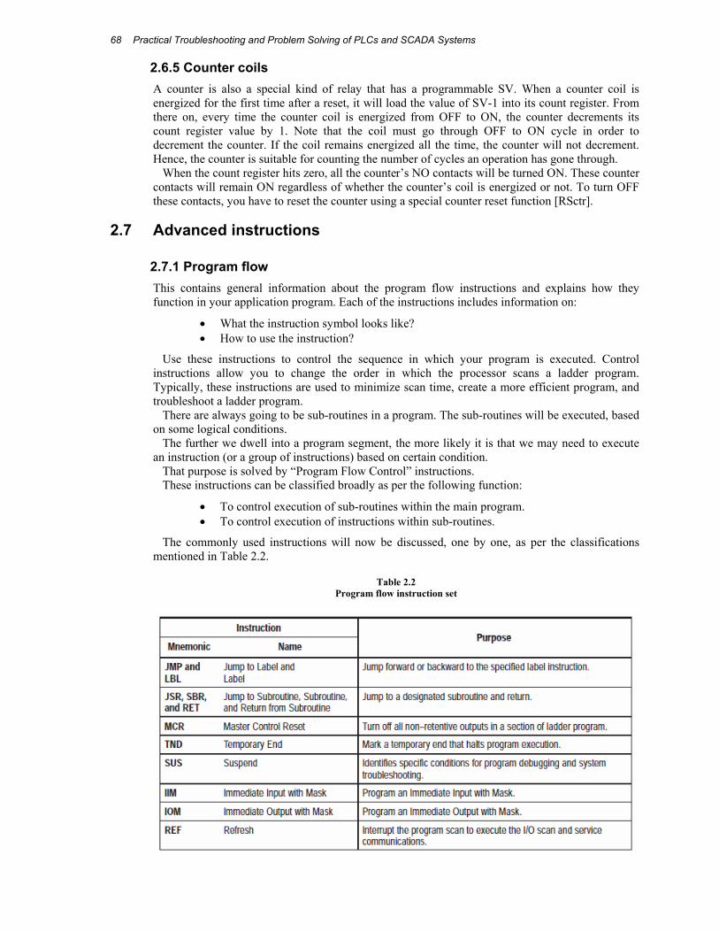
The commonly used instructions will now be discussed, one by one, as per the classifications mentioned in Table 2.2.

Table 2.2 Program flow instruction set


69

Usage of JMP The JMP instruction causes the controller to skip rungs. You can jump to the same label from one or more JMP instruction.

Jumping forward to a label saves program scan time by omitting a program segment until needed. Jumping backward lets the controller execute program segments repeatedly.

Be careful not to jump backward an excessive number of times. The watchdog timer could time out and fault the controller. Use a counter, timer, or the “program scan” register to limit the amount of time you spend looping inside of JMP/LBL instructions.

Usage of LBL This input instruction is the target of JMP instructions having the same label number. You must program this instruction as the first instruction of a rung. This instruction has no control bits.

You can program multiple jumps to the same label by assigning the same label number to multiple JMP instructions. However, label numbers must be unique.

Be careful not to jump (JMP) into an MCR zone. Instructions that are programmed within the MCR zone starting at the LBL instruction and ending at the “END MCR” instruction are always evaluated as though the MCR zone is true, regardless of the true state of the “Start MCR” instruction.

Usage of JSR, SBR, and RET The JSR, SBR, and RET instructions are used to direct the controller to execute a separate sub-routine file within the ladder program and return to the instruction following the JSR instruction.

If you use the SBR instruction, the SBR instruction must be the first instruction on the first rung in the program file that contains the subroutine.

Use a sub-routine to store recurring sections of program logic that must be executed from several points within your application program. A sub-routine saves memory because you program it only once.

Update critical I/O within sub-routines using immediate input and/or output instructions (IIM, IOM), especially if your application calls for nested or relatively long sub-routines. Otherwise, the controller does not update I/O until it reaches the end of the main program (after executing all sub-routines).

Outputs controlled within a sub-routine remain in their last state until the sub-routine is executed again.

Usage of MCR

Master Control (MC) This is one of the “Program flow control” instructions, but with a difference. It is used inside a program block or segment to control the execution of a group of instructions. The “Master control” (MC) instruction is typically used in pairs with a “Master control reset” (MCR) as shown in Figure 2.61.


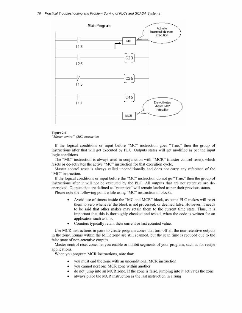
Figure 2.61 “Master control” (MC) instruction

If the logical conditions or input before “MC” instruction goes “True,” then the group of instructions after that will get executed by PLC. Outputs states will get modified as per the input logic conditions.

The “MC” instruction is always used in conjunction with “MCR” (master control reset), which resets or de-activates the active “MC” instruction for that execution cycle.

Master control reset is always called unconditionally and does not carry any reference of the “MC” instruction.

If the logical conditions or input before the “MC” instruction do not go “True,” then the group of instructions after it will not be executed by the PLC. All outputs that are not retentive are de-energized. Outputs that are defined as “retentive” will remain latched as per their previous status.

Please note the following point while using “MC” instruction in blocks:

• Avoid use of timers inside the “MC and MCR” block, as some PLC makes will reset them to zero whenever the block is not processed, or deemed false. However, it needs to be said that other makes may retain them to the current time state. Thus, it is important that this is thoroughly checked and tested, when the code is written for an application such as this.

• Counters typically retain their current or last counted value.

Use MCR instructions in pairs to create program zones that turn off all the non-retentive outputs in the zone. Rungs within the MCR zone are still scanned, but the scan time is reduced due to the false state of non-retentive outputs.

Master control reset zones let you enable or inhibit segments of your program, such as for recipe applications.

When you program MCR instructions, note that:

• you must end the zone with an unconditional MCR instruction • you cannot nest one MCR zone within another • do not jump into an MCR zone. If the zone is false, jumping into it activates the zone • always place the MCR instruction as the last instruction in a rung


71

The MCR instruction is not a substitute for a hard–wired master control relay that provides emergency stop capability. You still must install a hard-wired master control relay to provide emergency I/O power shutdown.

If you start instructions such as timers or counters in an MCR zone, instruction operation ceases when the zone is disabled. Re-program critical operations outside the zone if necessary.

Do not jump (JMP) into an MCR zone. Instructions that are programmed within the MCR zone starting at the LBL instruction and ending at the “END MCR” instruction are always evaluated as though the MCR zone is true, regardless of the true state of the “Start MCR” instruction. If the zone is false, jumping into it activates the zone from the LBL to the end of the zone.

The TOF timer activates when placed inside of a false MCR zone. The MCR instruction is not a substitute for a hard-wired master control relay. We recommend that your programmable controller system include a hard-wired master control

relay and emergency stop switches to provide I/O power shut down. Emergency stop switches can be monitored, but should not be controlled by the ladder program. Wire these devices as described in the installation manual.

SLC 5/03 and higher processors – When an online and an unmatched MCR instruction exists in your program, the END instruction acts as the second unconditional MCR instruction and all of the rungs following the first MCR instruction execute via the current MCR instruction state.

You can save the program while online if unattended MCR instructions exist. However, if you are offline and unattended MCR instructions exist, an error will occur.

Usage of TND This instruction, when its rung is true, stops the processor from scanning the rest of the program file, updates the I/O, and resumes scanning at rung 0 of the main program (file 2). If this instruction’s rung is false, the processor continues the scan until the next TND instruction or the END statement. Use this instruction to progressively debug a program, or conditionally omit the balance of your current program file or sub-routines.

If you use this instruction inside a nested sub-routine, execution of all nested subroutines is terminated.

Micro Logix 1000 controllers – Do not execute this instruction from the user error fault routine (file 3), high-speed counter interrupt routine (file 4), or selectable timed interrupt routine (file 5) because a fault will occur.

Usage of SUS When this instruction is executed, it causes the processor to enter the Suspend Idle mode and stores the Suspend ID in word 7 (S:7) of the status file. All outputs are de-energized.

Use this instruction to trap and identify specific conditions for program debugging and system troubleshooting.

When the SUS instruction is executed, the programmed ID as well as the program file ID from which the SUS instruction executed is placed in the system status file.

Usage of IIM This instruction allows you to update data prior to the normal input scan. When the IIM instruction is enabled, the program scan is interrupted. Data from a specified I/O slot is transferred through a mask to the input data file, making the data available to instructions following the IIM instruction in the ladder program.

For the mask, a 1 in an input’s bit position passes data from the source to the destination. A 0 inhibits data from passing from the source to the destination.

Usage of IOM This instruction allows you to update the outputs prior to the normal output scan. When the IOM

instruction is enabled, the program scan is interrupted to transfer data to a specified I/O slot through a mask. The program scan then resumes.

For the mask, a 1 in the output bit position passes data from the source to the destination. A 0 inhibits the data from passing from the source to the destination.


Usage of REF The REF instruction has no programming parameters. When it is evaluated as true, the program scan is interrupted to execute the I/O scan and service communication portions of the operating cycle (write outputs, service communications, and read inputs). The scan then resumes at the instruction following the REF instruction.

You are not allowed to place a REF instruction in a DII subroutine, STI subroutine, I/O subroutine, or user fault subroutine.

The watchdog and scan timers are reset when executing the REF instruction. You must insure that an REF instruction is not placed inside a non-terminating program loop. Do

not place an REF instruction inside a program loop unless the program is thoroughly analyzed.

2.7.2 Arithmetic or math instructions While performing manipulation of data, it is most likely that it may be necessary to perform some mathematical functions on data. Very rarely will the actual data be in the format that you require.

In some cases, “Math functions” are required to implement scientific formulae, which also happen to be one of the integral parts of any process control logic.

While using these instructions, it is very important that the programmer is well aware of all the number systems and the PCL storage register formats. Math functions operations are much easier to understand than the various types of formats used.

In general, it will be found that all PLC makes always include the following Math functions:

• Addition – The capability to add one data register to another. It is commonly called the “ADD” instruction.

• Subtraction – The capability to subtract one data register from another. It is commonly called the “SUB” instruction.

• Multiplication – The capability to multiply one data register with another. It is commonly called the “MUL” instruction.

• Division – The capability to divide one data register into another. It is commonly called the “DIV” instruction.

In addition to these basic instructions, advanced instructions are also available in programming languages.

For example, advanced functions that are commonly used in most PLC vendor programming languages are as follows:

• Sine • Cosine • Square root • Scaling • Absolute value • Tangent • Natural logarithm • Base 10 logarithm • X^Y (X to the power of Y)

Before going into the details of the instructions, it is necessary to first get acquainted with some important concepts. Any common math instruction will have the following:

Operand A – This is the first operand register, which contains value of the first operand. It may have a memory address of the operand (e.g., DB10.DW100) or a constant value (e.g., # 2100).

Operand B – This is the second operand register, which contains the value of the second operand. It may have a memory address of the operand (e.g., DB10.DW110) or a constant value (e.g., # 2200).

Destination register – This is the register where the result of the math operation will be stored. Since the result is to be stored, it will always need to be a register.

Once the basic components of a common math instruction have been fully understood, it is important to start thinking about registers. What exactly are the registers in the PLC?


73

Register: A register is simply a storage location in the PLC memory with a unique address. It has 16 bits, so it can hold a maximum value of “65535” (2^16=65536), provided all 16 bits are used. If one bit is assigned as a “sign” bit, then the value that can be held will be from “–32767 to +32767” (2^15=32767).

Suppose the numbers that need to be used in the math operation are larger than the above-mentioned limits, what will happen? That instruction will generate an “overflow” bit, and that bit will be set within PLC.

For handling larger numbers, a greater number of registers are provided. These are referred to as “Double Precision” math instructions.

Single-precision math instruction: It uses one register for each… That is, operand 1, operand 2, and destination register. A total of

three registers are used for a single math instruction. Double-precision math instructions: It uses two registers for each… That is, operand 1, operand 2, and Destination register. A total of

six registers are used for a single math instruction. Nowadays, all PLCs make use of floating-point math instructions as well. Floating-point math

instructions simply use decimal points in addition to “Double-precision Math” instructions. The floating or decimal value for operands can be specified. Similarly, the obtained result will

also be in decimal format. All larger PLC systems have floating-point math instructions, since this is required in most

formulae. Contrary to this, most micro/mini PLC systems do not have floating-point math instructions.

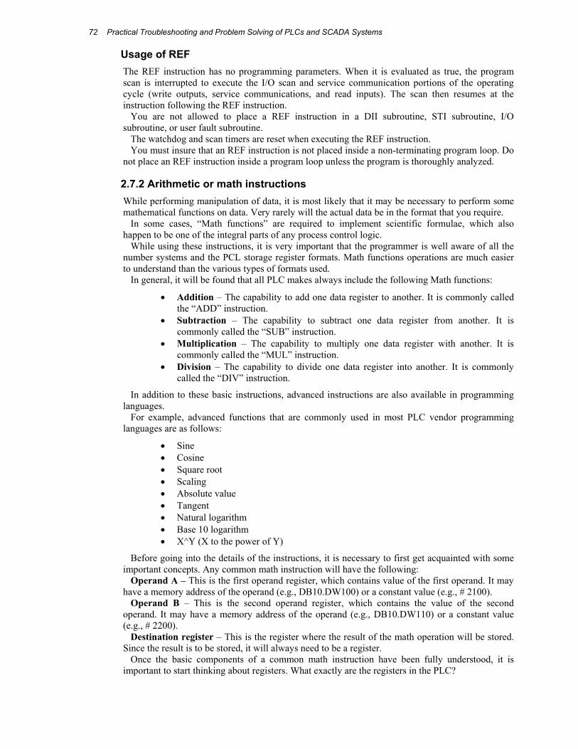
1. Addition (ADD) This is one of the most commonly used math instructions in program logic. In the following

example, operand 1 register value (DW100) is added with that of operand 2 register (DW110), and the result is stored in destination register DW220.

An “Enable” bit in previous rung decides whether to execute “ADD” instruction or not. Only if the “Enable” bit rung goes “True,” the addition instruction will be executed.

As seen before, if the “Enable” bit is not used, the formula would be executed on each and every scan.

In the following example, when input I3.3 goes “True,” only then “ADD” instruction will be executed as shown in Figure 2.62.

If the DW 100 location contains a value of “#2100”and DW110 contains “#2200,” then (after the addition) the result “#4300” will be stored in the DW220 register.

Figure 2.62 ADD instruction

If the result exceeds the destination register’s maximum limit as discussed earlier, then the “Overflow” bit will be set.

In some cases it may be found that, instead of specifying memory locations (DW100/DW110) in operand fields, direct constant values are specified.

For example, in operand 1 field, you may define value “#2100” immediately. Similarly, “#2200” can be defined in operand 2 field. In double precision “ADD” instructions, it will be found that


operand 1 and 2 are specified with two registers, each instead of one. Similarly, the result will also be stored in two registers.

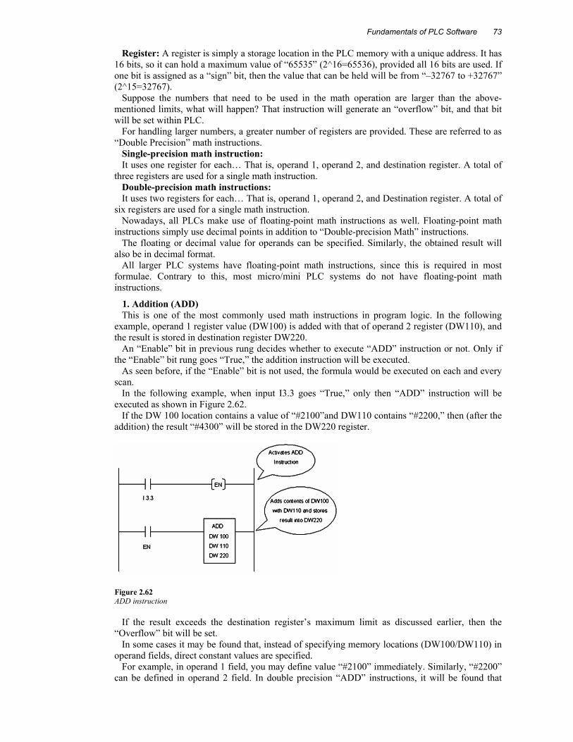
2. Subtraction (SUB) This is one of the commonly used math instructions in program logic for data manipulation. In

the following example, operand 1 register (DW210) value is subtracted from operand 2 register (DW200) and the result is stored in destination register DW220.

Figure 2.63 Subtraction instruction

Similar to the “ADD” instruction example, when input I3.3 goes “True” for “SUB” instruction then only it executes (Figure 2.63).

If DW 200 location contains value “#2200”and DW210 contains “#2100,” then after subtraction, the result “#100” will be stored in DW220 register. In the above case, “OP1>OP2” bit will get set and other two bits will remain false.

If the result were to have been negative, then the last bit “OP1<OP2” would have been set. Due to this feature of this instruction, it is often used both for the subtraction of two values as

well as for comparing them, at the same time. There is one very simple, but very important thing to note. In the “SUB” instruction, operand 2 is

always subtracted from operand 1. The logic should always be written, keeping this in mind.

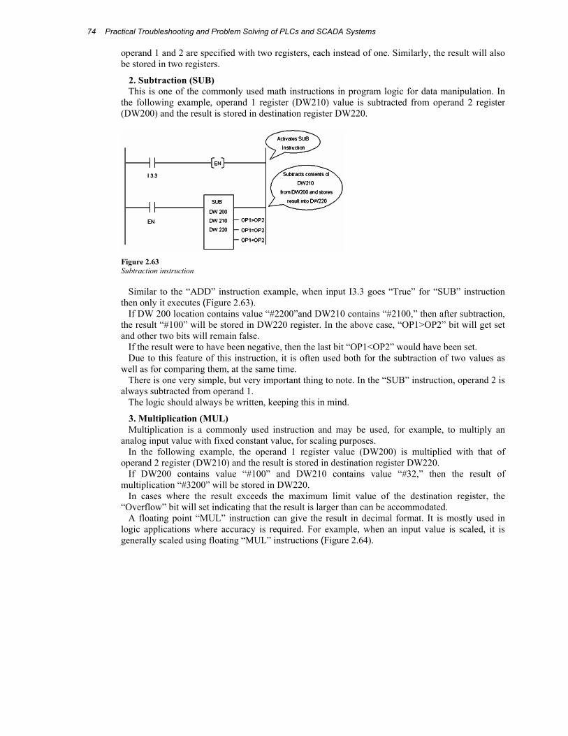
3. Multiplication (MUL) Multiplication is a commonly used instruction and may be used, for example, to multiply an

analog input value with fixed constant value, for scaling purposes. In the following example, the operand 1 register value (DW200) is multiplied with that of

operand 2 register (DW210) and the result is stored in destination register DW220. If DW200 contains value “#100” and DW210 contains value “#32,” then the result of

multiplication “#3200” will be stored in DW220. In cases where the result exceeds the maximum limit value of the destination register, the

“Overflow” bit will set indicating that the result is larger than can be accommodated. A floating point “MUL” instruction can give the result in decimal format. It is mostly used in

logic applications where accuracy is required. For example, when an input value is scaled, it is generally scaled using floating “MUL” instructions (Figure 2.64).


75

Figure 2.64 Multiplication instruction

4. Division (DIV) The division instruction is often used in conjunction with “MUL” instruction, for executing a

formula or dividing an analog input value by a fixed constant value, for scaling. In the following example, Operand 1 register value (DW200) is divided by operand 2 register

(DW210) and the result is stored in destination register DW220. If DW200 contains value “#100” and DW210 contains value “#5,” then the result of

multiplication “#20” will be stored in DW220. In case the result exceeds the maximum limit value of the destination register, the “Overflow” bit

will be set, indicating that the result is larger than that can be accommodated. At the same time, this bit also acts as an Error bit, if the Operand 1 is divided by zero.

If the remainder value is produced, then the “Remainder bit” will get set and the remainder will be stored in a register next to the destination register.

Figure 2.65 Division instruction

Depending on the make of the PLC, the storage location of the remainder value may differ. It is generally given clearly in the instruction set as shown in Figure 2.65.

There is one very simple, but very important thing to note with the “DIV” instruction. Operand 1 is always divided by operand 2.

Using these basic instructions, most logic functions, related to input/output access, data transfer, timers, counters, arithmetic formulae, and other common logic functions can be implemented easily and effectively.

When used frequently, they become easy to understand, and PLC programming takes on a whole new meaning.


2.7.3 Data load and transfer instructions As seen before, the PLC constantly collects various analog as well as digital data through numerous inputs. In order to use this data as and when it is required in a program, work needs to be done on the data.

This means that there is a need to organize the data and, if necessary, carry out some manipulation using appropriate instructions or blocks that are available.

During each program execution cycle, the PLC stores input and output statuses in a “Process Image Table.” During each execution cycle, this table will get filled up with new values. As a result of this, it is important that before the data gets lost, it is moved to some place and stored.

To accomplish this, some PLCs make use of two different instructions whereas others perform this with a single instruction.

Figure 2.66 shows the schematic of “Data Load and Transfer” operation.

Figure 2.66 Data load and transfer

As shown in Figure 2.66, data is gathered from an “Input Image Table” (PII) using the “Load” instruction into accumulator first, which acts as a temporary storage area. Next, it is transferred to storage registers (data blocks). After being processed, it is passed on to the “Output Image Table” (PIQ), and then given finally to the field, through a module.

1. Load (LD) This is a very commonly used instruction for “getting” the data in an accumulator or a temporary

storage area. It is basically used for “collecting” the data from an PII, accumulator and data registers. This

instruction is used along with the reference of the location from where the data have to be collected.

For example, in Figure 2.66, instruction “L IW2” has been used. This means that the input word with module address “2” will be collected and stored in the accumulator. Immediately after this has been concluded, the bit status of “IW2” is available with the accumulator (temporary storage), and it now can be used either for data manipulation or for further permanent storage.

For the reading of analog input values, you may find the same instruction but with different syntax such as “L PIW128” as used in the SIEMENS PLC range. This means that the data available at the analog input channel with address 128 will be gathered into an accumulator.

This data can now be processed further or stored in data registers. This instruction is commonly used for loading timers and counters values.

2. Transfer (T) This instruction is used, in conjunction with the “LOAD” instruction, to transfer data collected to

another place. It is basically used for “transferring” the data in between the accumulator, data registers, and the output image table (PIQ).

Similarly to the “LOAD” instruction, it is also used along with a reference of the location to where the data has to be transferred.


77

For example, in Figure 2.66, the instruction “T QW2” has been used. This means that the accumulator contents will be transferred to output image address “QW2.”

Following this, the bit status of “QW2” will change as per the bit status of the accumulator (temporary storage) word.

For analog output value transfers, it is possible to find the same instruction, but with different syntax such as “T PQW128” for SIEMENS PLC. In this example, it means the data available within the accumulator will be transferred to the analog output channel by means of the PQW128 instruction.

This instruction is also used for transferring parameters related to timers, counters, etc.

3. Move (MOV) Some PLC suppliers, who use a single instruction, perform the entire operation of the two

separate instructions, just discussed above. These two instructions are combined together as “MOV” to accomplish the final result.

The “MOV” instruction is always accompanied by a “Source” location (register) address and a “Destination” location (register) address, so that the instruction transfers the contents from the

“Source” to the “Destination” register.

Figure 2.67 Data move instruction

Depending on the PLC instruction set, the “MOV” instruction can be used for transferring words, double words, and real data from one location to another.

As shown in Figure 2.67, “MOV” instruction transfers data from source location “IW2” to “QW2”, but only when input “I1.3”goes “True.”

Otherwise, the data will not be transferred. This is done meticulously to transfer the data only under particular conditions, but this may not always be the case.

Some PLC vendors have instruction “MOVBK” (move block), which is an extended version of the above instruction. Using this instruction, it is possible to transfer the contents of group of data registers to another group of data registers.

To accomplish this, along with source and destination addresses, one additional parameter needs to be specified. This is the “Length” of registers, so the PLC understands the number of registers that have to be transferred from the source to the destination.

Some PLC vendors also include an instruction “MOVN” (move not). It performs the same function as the “MOV,” but transfers the data in inverted form.

If the source location data bit was “1,” then “0” is moved to destination location data bit. Similarly, if the bit was “0,” then “1” is moved at the destination location.


2.8 Startup/shutdown/fault routine

2.8.1 Reference-PLC 5 The processor runs a fault routine, when it detects a major fault. The processor interrupts the current program, runs the fault routine, and resets the conditions for running your process. Once it is done by the processor, it continues with the original program.

You can use a fault routine to specify how a processor responds to a major fault. You can also use a fault routine to provide protection from powering up in run mode when the processor recovers from a power loss.

Responses to a major fault: When the processor detects a major fault, the processor immediately interrupts the current

program. If a fault routine exists (specified in S:29 as a fault routine), the processor runs that fault routine program.

Depending on the type of fault, the processor:

• returns to the current ladder program file if the processor can recover from the fault • enters fault mode if the processor cannot recover from the fault.

For example, the following rung includes an instruction that causes a major fault as shown in Figure 2.68:

Figure 2.68 Cause of major fault instruction

In the example above, the processor runs the fault routine after detecting the fault. If the fault routine resets the faulted bits, the processor returns to the next instruction in the program file following the one that faulted (instruction B) and continues executing the remainder of the rung.

If you do not program a fault routine for fault B, the processor immediately faults. The bits in word 11 of the processor status file indicate the type of major fault. Table 2.3

describes the fault associated with each bit.


79

Table 2.3 Bit fault status


2.8.2 Major fault codes Table 2.4 lists major fault codes. The processor stores the fault code in word 12 of the processor status file.

Table 2.4 Major faults


81

Table 2.4 Major faults-continued




83


2.8.3 Programming a fault routine If you choose to program a fault routine, first examine the major fault information recorded by the PLC–5 and decide whether to do the following before the PLC–5 processor automatically goes to the fault mode:

• set an alarm • clear the fault • shutdown in an orderly manner

Upon detecting a major fault, the processor immediately suspends the program file it was running and, if programmed, runs the fault routine file once to completion. If the processor does not run a fault routine, or the fault routine does not clear the fault, the processor automatically switches to fault mode.

2.8.4 Set an alarm You may need an alarm to signal when a major fault occurs. Put this rung first in your fault routine program and combine it with a counter as shown in Figure 2.69.

Figure 2.69 Alarm-fault routine

You can also set an alarm in your fault routine to signal when the fault routine clears a major fault.

2.8.5 Clearing the fault If you decide to clear the fault in the fault routine, place the ladder logic for clearing the fault at the beginning of the fault routine. You can compare the fault code with a reference.

2.8.6 Compare the fault code with a reference Identify the possible major faults and then select only those your application will let you safely clear. These are your reference fault codes.

From the fault routine, examine the major fault code that the processor stores in S:12. Use an FSC instruction to compare the fault code with the reference file that contains “acceptable” fault codes (word-to-file comparison). If the processor finds a match, the FSC instruction sets the found


(FD) bit in the specified control structure. Use a CLR instruction to clear the fault in S:11. Then, jump to the end of the fault routine to quickly complete running the fault routine.

In Figure 2.70, #N10:0 is the reference file.

Figure 2.70 Comparing fault code with reference

The processor completes the scan of the fault routine. If the routine clears S:11, the processor returns to the program file and resumes program execution. If the fault routine does not clear S:11, the processor executes the rest of the fault routine and goes into FAULTED mode.

Note: If the fault routine clears the major fault, the processor completes the fault routine and returns to the next instruction in the program file after the one that contained the faulted instruction. The remainder of the rung with the faulted instruction is executed as if the rung were false. It appears that the fault never occurred. The cycle of recurring fault routine execution continues until you correct the major fault.

2.8.6 Using shutdown logic Shutdown programming considerations should include the following:

• store initial conditions and reset other data to achieve an orderly start-up later • monitor the shutdown of critical outputs. Use looping if needed to extend the single

fault routine scan time up to the limit of the logic processor watchdog timer so your program can confirm that critical events took place

2.8.7 Testing a fault routine To test a fault routine, use a JSR instruction to the fault routine. Send a fault code as the first parameter of the JSR instruction. The processor stores the fault code in status word 12 and sets the corresponding bit in word 11.


85

You may detect and set your own faults using fault codes 0–9 or by using the processor-defined fault codes 12–80.

2.8.8 Setting up a fault routine You can write multiple fault routine programs and store them in multiple fault routine files, but the logic processor runs only one fault routine program when the PLC–5 detects a major fault. The number of the fault routine the PLC–5 runs is stored in word 29 of the processor status file. Typically, you enter a fault routine file number with the programming software and change the specified fault routine file from the ladder program.

To set up a fault routine, you need to:

• enable the fault routine • change the specified fault routine from ladder program, if necessary • create the program file and enter fault routine logic.

2.8.9 Enabling a fault routine To enable a fault routine, store the program file number (3–1999), of the file that contains the fault routine logic, in word 29 of the processor status file. When the processor encounters a major fault, the processor runs the fault routine logic to handle the fault.

If you do not specify a program file number, the processor immediately enters fault mode after detecting a fault.

2.8.10 Changing the fault routine from ladder logic You can change the specified fault routine from ladder logic by copying a new fault routine file number into word 29 of the processor status file.

Figure 2.71 shows an example program for changing the fault routine file number.

Figure 2.71 Changing fault routine file number

Be sure neither to corrupt the program-file number of the fault routine, nor use the same file for any other purpose. If the file number you specify results in a nonexistent fault routine, the processor immediately enters the fault mode after detecting a fault. Unexpected machine operation may result in damage to equipment and/or injury to personnel.

2.8.11 Clearing a major fault You can clear a major fault with one of the following methods:

• use the programming software to clear the major fault

For more information on using the programming software to clear major faults, see the PLC–5 A.I. Series Software Reference manual.

• turn the key switch on the PLC–5 processor from REM to PROG to RUN.

Note: Clearing a major fault does not correct the cause of the fault. The PLC–5 processor might continue to repeat the fault cycle until you correct the cause(s) for the major fault.


2.8.12 Setting power-up protection You can set your processor so that after a power loss the processor does not come up in run mode. Bit 1 in word 26 of the processor status file sets power-up protection. Table 2.5 shows the states for this bit.

Table 2.5 Power-up protection status

Set word 26, bit 1 manually from the processor status screen (see the PLC–5 A.I. Series Software Reference manual), or you can latch this bit through ladder logic. When set, the processor scans the fault routine once to completion after the processor recovers from a power loss.

You can program the fault routine to determine whether the processor’s status will let the processor respond correctly to ladder logic and whether to allow or inhibit the startup of the processor.

2.8.13 Allowing or inhibiting startup Bit 5 of status word 11 controls whether the processor can start up after a power loss. After a power loss, the processor automatically sets this bit. Table 2.6 shows how you can change this bit from your fault routine.

Table 2.6 Startup status after power loss

Note you can use JMP and LBL instructions to scan only the portion of the fault routine associated with a particular fault or power-up condition.

2.9 The seven good habits of PLC programming 4. Write your code in Ladder Logic all the time unless you have to write long

mathematical formulae. Ladder Logic is easy on the eyes and following the flow of logic is a quick process. While monitoring the Ladder Logic, you can simply use a red or green color to see if a rung in the ladder is continuous or broken. You will be amazed how fast you can go through the ladder logic code and troubleshoot the program; something that is almost impossible to do with STL code. A well-written PLC code can save lots of money for a company, not only when the production line is running perfectly, but also when the line is down.

5. Keep the group of the related code as short as possible. The longer it gets the harder it will be to troubleshoot it later. We all read the newspaper every morning and listen to the news on the radio. Which one do you prefer, the short radio news or the longer newspaper?


87

6. Comment, comment, and comment. Write comments as much as you can. Because you know what you are doing, it does not mean that everybody else should understand it easily and quickly. Programmers mainly live with their PLC code during the stage of writing and implementing it, which is the big killer for writing comments. A programmer always has the whole picture in his/her mind, which probably encourages him/her not to write comments. Even a few words are better than no words. A year from now you will be asked to look back at the same code to re-use it. You will appreciate any comments in the code especially for the tricky parts.

7. Make it hard on yourself and easy on the rest. Programming is like writing instructions for operating a new tool or know how for troubleshooting a new machine. Prevent writing complicated or complex code. Most of the time, the machine’s operation is complex. Please do not make it worse.

8. Plan any code writing on paper first. Resist the tempting desire of writing the code on the fly and hope that it comes together eventually. Believe me that this won’t go well eventually. Programming is like writing a report, a thesis, or a book. You lay out the body first, then you proceed to the main functions and sub-functions after that. If you have a map for what you are doing, you will make it easy not only on yourself but also on whoever looks at that code later. Having a good foundation in place will always make any addition or deletion easily and everyone can follow it.

9. Before writing PLC code, prepare a list of all functions that will be necessary to get the project done. Leave spares here and there, so you stay organized later when you are adding new functions. Assign space to flags and keep the related flags together as a group. This will help a lot when you have to use one function five times with five different groups of flags. You will be amazed at how fast and clean you will be able to put the code together.

10. Back up the files. Add a revision and date to the PLC code. Document all the changes. You should make a backup of the online code all the time before applying any changes to the code. That is called “establishing your point of return.” You can always go back to where you were in case your changes do not go as planned. After you are done with the PLC code make a backup, add a revision, add comments, and add date. This way you can always tell what this file is for and when the changes have happened. Create a log of whatever happened and what you did to fix it in case you are troubleshooting the PLC code. Not only you are keeping a good record, but also you can use this log for your service report to your manager or customer instead of wondering later what you did or what you should write in your report.


Date post:	20-Apr-2020
Category:	Documents
Upload:	others
View:	32 times
Download:	0 times

Fundamentals of PLC Software · Fundamentals of PLC Software 37 The “L1” and “L2”...

Documents