1All instruments are designed to take advantage of some molecular property or behavior. For example, chromatography is based on the different strength of intermolecular interac-tions that molecules have with mobile and stationary phases. Electrochemistry is based on the ability of molecules to gain or lose electrons. In this book, we focus on the fact that atoms and molecules absorb and emit electromagnetic radiation (EMR). By measuring the amount and the characteristics of the EMR absorbed and emitted, we can measure the concentration of particular molecules present in a sample or gain structural information about them. You may already be familiar with several of the instrumental methods used to measure the absorption and emission of electromagnetic radiation, such as UV‐visible, infrared (IR), and fluorescence spectroscopy.
In order to better understand the fundamental basis of these techniques, in this chapter we examine the properties of electromagnetic radiation and its effects on atoms and molecules. In subsequent chapters, we examine specific spectroscopic techniques. While all the techniques share common features, the specific instruments required and the information we gain from each are quite different and therefore require individual examination.
1.1. PROPERTIES OF ELECTROMAGNETIC RADIATION
Spectroscopic methods ultimately rely on measuring characteristics of electromagnetic radiation, which travels through space as a wave, as shown in Figure 1.1. As the name implies, it has two components, an electric field and a magnetic field, which are at right angles to one another. Figure 1.1 shows only a single wave with its electric field oriented along the x‐axis, but in reality, most sources of electromagnetic radiation, like light bulbs and car headlights, emit radiation in which the electric field of the waves are randomly distributed around the x‐axis. For now, however, we take a simplified view by focusing on only a single electromagnetic wave.
FUNDAMENTALS OF SPECTROSCOPY
0003959059.INDD 1 09/03/2018 8:16:56 AM
COPYRIG
HTED M
ATERIAL
2 SPECTROSCOPY
All electromagnetic waves have the properties of:
1. Speed2. Amplitude3. Frequency4. Wavelength5. Energy
Each of these characteristics is described below.
1.1.1. Speed, c
Electromagnetic radiation in a vacuum travels at 2.998 × 10⁸ m/s, commonly referred to as the speed of light, c. This speed only pertains to light traveling in a vacuum, though, because EMR slows down when it travels through matter such as air and water. We dis-cuss the speed of light when it travels through matter in a later section.
1.1.2. Amplitude, A
The amplitude, A, of a wave is the maximum length of the electric field vector, as shown in Figure 1.2. We seldom consider the amplitude of the wave because detectors are not fast enough to measure the magnitude of the electric field vector. Instead, we measure the radiant power, P, of a beam, which is proportional to the square of the amplitude. Radiant power is the amount of energy transmitted per unit time and is given by Eq. (1.1), where E is the energy of a photon and ϕ is the flux (i.e., the number of photons per unit time) [1]:
P E (1.1)
Electromagnetic wave
Magnetic field (B)
Electric
field (E)
Propagationdirection
Wavelength (λ)
⇀
⇀
FIGURE 1.1 Diagram of a single electromagnetic wave propagating through space. The diagram indicates that an electromagnetic wave has both an electric field (E) and magnetic field (B) associated with it and that they are oriented at right angles to each other. It also indicates that the wavelength (λ) is the distance the wave travels during one oscillation of the electric and magnetic fields. Source: Reproduced with permission of Eric Clarke.
0003959059.INDD 2 09/03/2018 8:16:57 AM
FUNDAMENTALS OF SPECTROSCOPY 3
Although radiant power is commonly referred to as intensity, I, intensity is strictly defined as the radiant power from a point source per unit solid angle, usually measured in watts per steradian [1, 2].
1.1.3. Frequency, υ
Frequency, υ, is the number of oscillations a wave makes per unit time and is typically measured in hertz, Hz, with units of reciprocal seconds, 1/s or s−1. To visualize the physical meaning of frequency, imagine sitting on a rock out in the ocean with a stop-watch and counting waves that pass the rock. If you count, say, 120 waves in a minute, the frequency is
1201
160
12060
2 0 1wavesminute
minuteseconds
wavesseconds
s o. rr Hz2 0.
In other words, two waves pass the rock every second. If more waves pass every second, the frequency is higher, and fewer waves per second are associated with a lower frequency.
The speed and wavelength of electromagnetic radiation change as it passes through different media, but the frequency remains the same. As described below, the frequency of EMR is closely related to the energy of the EMR. Therefore, the frequency is the characteristic that truly differentiates one wave from another.
1.1.4. Wavelength, λ
The wavelength, λ, is the peak‐to‐peak distance of the wave, as shown in Figure 1.2. Because it is a distance, wavelengths are typically measured in meters. For example, EMR in the visible portion of the electromagnetic spectrum has wavelengths between 380 and 760 nanometers (nm).
1.1.5. Energy, E
As we will see in all of the subsequent chapters, energy is really the fundamental wave characteristic that matters most in terms of the impact electromagnetic radiation has on matter. We often talk about EMR in terms of wavelengths, frequencies, and wavenumbers,
Amplitu
de
Wavelength
FIGURE 1.2 A side view of the electric field component of an electromagnetic wave as it propa-gates from left to right across the page. The amplitude is the displacement along the y‐axis and the wavelength is the peak‐to‐peak distance between a single oscillation of the wave.
0003959059.INDD 3 09/03/2018 8:16:57 AM
4 SPECTROSCOPY
but these ultimately relate to energy. In order to understand the energy of radiation, we must consider the wave/particle duality of light. When EMR propagates through space, it is convenient to focus on its wave properties (frequency, wavelength, amplitude). However, when it interacts with matter, it is useful to think of EMR as a discrete particle that contains a fixed amount of energy that can be transferred to an atom or molecule. That discrete particle is called a photon.
The energy that a photon contains is directly related to its frequency and wavelength, as shown in the two relationships in Eqs. (1.2) and (1.3):
E h (1.2)
Ehc
(1.3)
where h is Planck’s constant (6.626 × 10⁻³⁴ Js) and c is the speed of light (2.998 × 10⁸ m/s). These equations are fundamental to the study of spectroscopy. They also clearly show that photons with higher frequencies (i.e., faster oscillations) and shorter wavelengths are higher in energy than those with slower oscillations and longer wavelengths (see Figure 1.3). To help make a mental association between these relationships, consider the two waves shown in Figure 1.3. Imagine trying to draw a wave of each frequency across the entire length of a chalkboard or white board, and that you only have 15 seconds to go from one end of the board to the other. You have the same amount of time in each case because light propagates through space at the same velocity regardless of wavelength. Clearly, the higher frequency wave – the one with little space between peaks and therefore
Long wavelength
Low frequencyLow energy
High frequencyHigh energy
Short wavelength
FIGURE 1.3 Depiction of the reciprocal relationships between wavelength and frequency. Longer wavelengths are associated with lower frequencies and lower energies, while shorter wavelengths are associated with higher frequencies and higher energies.
0003959059.INDD 4 09/03/2018 8:16:58 AM
FUNDAMENTALS OF SPECTROSCOPY 5
shorter wavelength – will require you to expend a greater amount of energy to fill the board, whereas you can take a leisurely stroll (i.e., exert low energy) along the board when drawing the low‐frequency, long‐wavelength wave.
From the fact that Eqs. (1.2) and (1.3) are equal to each other, we can see that
c (1.4)
This relationship has implications for the speed and wavelength of EMR as it travels through different media such as air, water, benzene, etc. As radiation passes through matter, its electric field interacts with the electrons in the matter, slowing its propagation, meaning that the speed of light is different in different media. In a vacuum, the speed is 2.998 × 10⁸ m/s, but in everything else, including air, it is slower. However, as the EMR propagates through matter, its frequency is unaffected, so υ remains the same. In order to maintain the equality in Eq. (1.4), when the speed, c, decreases, then the wavelength must also decrease in order to maintain a constant frequency, υ.
The change in the speed of EMR in matter is measured by the refractive index of a substance, η, where
ccv
i (1.5)
in which cv is the speed in a vacuum and ci is the speed in the substance of interest. Because EMR is slower in matter than it is in a vacuum, such that ci < cv, refractive indices are greater than 1.00. The velocity of radiation in air is within 1% of the velocity in a vacuum such that using c = 2.998 × 10⁸ m/s does not generally lead to significant bias in calcula-tions for many of the situations in which we are interested.
It should be noted that the measurement of η depends on the frequency of the EMR used and the temperature. In order to standardize the measurement, the frequency of 5.09 × 10¹⁴ Hz (equivalent to 589 nm wavelength light), which is a frequency emitted by excited sodium atoms, is typically used, and values are often measured at 20 °C [3]. The symbol D
20 (or D25 if values are measure at 25 °C) is often used to denote refractive
indices, with the superscript specifying the temperature at which the measurement was made, and the subscript indicating that the sodium D line was used. Some values for common materials are given in Table 1.1 [4–7]. Notice that substances with π‐electrons such as toluene, and those with highly polarizable atoms like diiodometh-ane, have higher refractive indices, meaning that they slow the propagation of EMR more than other substances. Ultimately, the decrease in speed is due to polarization of the atoms and molecules in the material caused by the incoming electric field. The result is a temporary deformation of the electron clouds associated with the atoms or molecules. The energy of the light is then re‐emitted by the atoms or molecules with the same frequency, but its progress (i.e., speed) has been slowed by the temporary retention by the material. It is interesting to note that scientists have slowed the speed of light down to a mere 38 miles‐per‐hour – a typical speed for a car – using Bose–Einstein condensates [8].
0003959059.INDD 5 09/03/2018 8:16:58 AM
6 SPECTROSCOPY
1.1.6. Wavenumber,
While frequency and wavelength are commonly used to describe EMR, the wavenumber, , is also used, particularly when dealing with infrared spectra. The wavenumber is
related to energy as shown in the first relationship in Eq. (1.6):
E hc hhc (1.6)
TABLE 1.1 Refractive Indices of Some Common Materials
a A polymer film made with a pattern of thin aluminum shapes (see Ref. [4]); measured at 0.3 THz.
Calculate the speed of EMR in diamond.
Answer:
cc
c
c
v
i
diamond
diamond
m/s
m/s
2 4172 998 10
2 998 102 417
8
8
..
..
1 240 108. m/s
Another question:Calculate the speed of EMR in the metamaterial listed in the table.
Answer:7.77 × 10⁶ m/s.
EXAMPLE 1.1
0003959059.INDD 6 09/03/2018 8:16:59 AM
FUNDAMENTALS OF SPECTROSCOPY 7
Wavenumbers are typically measured in units of reciprocal centimeters, cm−1, meaning that they express the number of oscillations that occur per centimeter. Equation (1.7) shows how wavenumbers are related to frequency and wavelength:
c1 (1.7)
While it may seem unnecessary to have three different parameters to describe EMR – frequency, wavelength, and wavenumber – different fields of spectroscopy, for reasons of convenience and historical legacy, use different measures. For example, in UV‐visible spectroscopy we usually deal in wavelengths, whereas wavenumbers are commonly used in IR spectroscopy. Of course they are all interchangeable, but to work in any of these fields requires fluency in all three parameters.
1.2. THE ELECTROMAGNETIC SPECTRUM
In this section, we explore how atoms and molecules interact with incoming EMR. Specifically, we look at the range of energy carried by electromagnetic radiation of different frequencies and the effects that photons with different energy have on matter.
Calculate the energy, frequency, and wavenumber of EMR that has a wavelength of 1.234 μm.
Answers:
Ehc 6 626 10 2 998 10
1 234 101 610 10
34 8
619
. .
..
Js m/s
mJJ
m/sm
s Hzc 2 998 10
1 234 102 429 10 2 29 10
8
614 1 14.
.. .4
1 11 234 10
8 104 1065 1
..
mm
Another question:Calculate the energy, wavelength, and frequency associated with EMR with a wavenumber of 543.2 cm−1. Be careful with units.
Answers:
E 1 079 10
1 841 10 18 41
1 628 10 16 28
20
5
13 1
.
. .
. .
J
m
s TH
m
zz
EXAMPLE 1.2
0003959059.INDD 7 09/03/2018 8:16:59 AM
8 SPECTROSCOPY
By measuring these various effects, we learn about the properties of the matter we are analyzing. This is critical, as the different regions of the spectrum ultimately relate to the different spectroscopic techniques described in the coming chapters. The different energies also require significantly different types of detectors, optical components, and mathematical treatment of data in order to make the measurements from which we ultimately gain chemical information.
The electromagnetic spectrum is shown in Figure 1.4.One of the ways atoms and molecules interact with electromagnetic radiation is to
absorb it. This occurs because atoms and molecules can exist in different states that have different, but quantized, energy levels (see Figure 1.5). If the energy of incoming EMR matches the energy difference (ΔE) between two quantum states, then the radiation can be absorbed. This process forms the basis for all common forms of spectroscopy, including UV‐visible, IR, and NMR spectroscopy, and is discussed in greater detail later in this chapter and in Chapters 2 and 3.
Figure 1.5 depicts a quantized, electronic transition [9]. In this case, an electron is promoted from a bonding to an antibonding orbital, denoted as π and π*‐orbitals, respec-tively. Many other types of quantized transitions involving different types of orbitals (e.g., σ‐, σ*‐, and n‐orbitals) can occur. What is common to each is that the ground and excited states are separated by a fixed energy difference, ΔE. An atom or molecule can absorb an incoming photon if the energy of the photon matches ΔE. In the process, the absorbed energy changes the molecule, for example, by causing a nuclear spin flip as occurs in NMR spectroscopy, an increase in the amplitude of bond vibrations as occurs in IR spectroscopy, or a change in the electron distribution as depicted here for UV-visible spectroscopy.
When thinking about the energy range associated with each region, it is helpful to consider the energy required to break a typical carbon–carbon (C─C) bond, which is approximately 5.8 × 10⁻¹⁹ J (based on the bond energy of approximately 350 kJ/mol). Comparing the photon energies to this bond strength gives some sense of the energy being carried by different photons. Photons with less energy cannot break bonds but can cause other lower energy phenomenon to occur, while those with higher energy can break bonds, which causes significant molecular rearrangements or ionizes atoms and molecules.
1.2.1. Radio-Frequency Radiation (10−27 to 10−21 J/photon)
The low‐frequency, long‐wavelength end of the spectrum is known as the radio‐ frequency range. The waves here are on the order of 0.1 mm to 100 meters in length (i.e., a tiny fraction of an inch to approximately 1 football field) or longer according to the ISO (International Organization for Standardization) definitions of the regions of the electromagnetic spectrum (although we note that the ranges specified seem to allow for some overlap between regions) [10–13]. Recalling the reciprocal relationship between wavelength and energy means that this long‐wavelength radiation has exceptionally low energy, which is fortunate for us as radio waves fill the environment and are constantly passing through and around us. There is nothing in our bodies that absorbs this radia-tion, so it does not have any physiological effect, and we can therefore use it to broadcast radio and television signals.
0003959059.INDD 8 09/03/2018 8:16:59 AM
Mic
row
aves
Infr
ared
Ultr
avio
let
X-r
ays
α-, β
-, a
nd γ
-ra
diat
ion
Low
ene
rgy
(10–2
7 J)
Long
wav
elen
gth
(100
m)
Low
freq
uenc
y (1
06 H
z)
Hig
h en
ergy
(10
–11
J)
Sho
rt w
avel
engt
h (1
0–14
m)
Hig
h fr
eque
ncy
(1022
Hz)
Ele
ctro
n vi
brat
ions
that
ar
e re
spon
sibl
e fo
r ra
dio
and
TV
tran
smis
sion
Nuc
lear
spi
n fli
psin
NM
R s
pect
rosc
opy
Ele
ctro
n sp
in fl
ips
in
elec
tron
spi
n re
sona
nce
sp
ectr
osco
py
Incr
ease
s in
mol
ecul
ar
rota
tiona
l ene
rgy
Incr
ease
d am
plitu
de o
fm
olec
ular
str
etch
ing
and
bond
vib
ratio
n m
otio
ns Red
istr
ibut
ion
of
vale
nce
elec
tron
s in
to h
ighe
r en
ergy
orbi
tals
Red
istr
ibut
ion
of
vale
nce
elec
tron
s in
to h
ighe
r en
ergy
or
bita
ls
Pos
sibl
e bo
nd
brea
king
Pos
sibl
e bo
nd b
reak
ing
and/
orej
ectio
n of
ele
ctro
ns fr
om
atom
s or
mol
ecul
esIo
nizi
ng a
nd p
enet
ratin
gra
diat
ion
asso
ciat
ed
with
nuc
lear
pro
cess
es
Vis
ible
Rad
io w
aves
FIG
UR
E 1.
4
The
reg
ions
of t
he e
lect
rom
agne
tic s
pec
trum
and
the
eff
ect
that
rad
iatio
n in
eac
h re
gio
n ha
s on
mat
ter.
Not
e th
e la
bels
on
the
top
left
an
d r
ight
ind
icat
ing
tha
t th
e d
iag
ram
goe
s fr
om lo
w e
nerg
y el
ectr
omag
netic
rad
iatio
n (E
MR)
on
the
left
to
hig
h en
erg
y el
ectr
omag
netic
rad
iatio
n on
th
e rig
ht.
Als
o no
te t
he r
ecip
roca
l re
latio
nshi
p b
etw
een
ener
gy
and
wav
elen
gth
. Lo
ng (
i.e.,
hig
h va
lue)
wav
elen
gth
pho
tons
on
the
far
left
of
the
dia
gra
m h
ave
very
low
ene
rgy,
and
sho
rt w
avel
eng
ths
pho
tons
(far
rig
ht o
n th
e d
iag
ram
) hav
e ve
ry h
igh
ener
gy.
The
hig
h en
erg
y as
soci
ated
with
sho
rt
wav
elen
gth
pho
tons
mak
es t
hem
cap
able
of s
igni
fican
t d
amag
e to
mol
ecul
es a
nd t
hus
sig
nific
ant
neg
ativ
e he
alth
eff
ects
.
0003959059.INDD 9 09/03/2018 8:17:00 AM
10 SPECTROSCOPY
The EMR used in nuclear magnetic resonance (NMR) spectroscopy is in the radio‐fre-quency range, toward the shorter wavelengths (~0.3 to 0.8 m). Molecules are made of atoms, and atoms contain nuclei, some of which behave as if they are spinning. When placed in a magnetic field, the spins orient with or against the field, known as “spin‐up” or “spin‐down” orientations. The spin states have slightly different energies. Therefore, when EMR in the low energy, radio‐frequency range interacts with nuclei, the nuclei can absorb it. The energy of the EMR is used to change the spin of a nucleus from spin‐up (lower energy state) to spin‐down (higher energy state). The energy required to do this is almost trivial: approximately 2 × 10⁻²⁵ Joules per nucleus, six orders of magnitude (one million times) less than that of a C─C bond. Yet, as you may already know, NMR spectros-copy provides valuable information about molecular structures. It is hard to imagine modern chemistry without this technique. So while the energy of the radiation is quite low and the effect it has on matter – a mere nuclear spin flip – is almost imperceptible, this is an important region of the spectrum for chemists.
1.2.2. Microwave Radiation (10−23 to 10−22 J/photon)
The microwave region overlaps with the higher frequency portion of the radio wave region, but the two regions are generally distinguished by the technologies used to measure them. The microwave region is associated with two types of spectroscopy: (1) electron spin resonance (ESR) and (2) microwave spectroscopy. The basis of ESR
Ground state
Excited state
Energy ΔE
R R
R R
C
C C
CR R
R R
π-orbital
π*-orbital
π* transitionπ
FIGURE 1.5 Depiction of a π–π* transition (left) and the associated energy change, ΔE (right). Note that in the ground state, the electrons in the π‐orbital connect both carbon atoms above and below the plane of the bond. The electrons in the π‐bond are thus delocalized and shared between both carbon atoms. In the excited state, the π*‐orbitals, and thus the electrons in them, are localized on a specific carbon atom. Shared electrons like those in the ground state lower the energy of a molecule compared to localized electron density like that seen in the excited state. In order to transition from the ground state to the excited state, the molecule must absorb a photon that has an energy that exactly matches the energy difference (ΔE) between the ground and excited states.
0003959059.INDD 10 09/03/2018 8:17:02 AM
FUNDAMENTALS OF SPECTROSCOPY 11
spectroscopy is that electrons, like nuclei, have the property of spin‐up or spin‐down, which have slightly different energies when samples are placed in a magnetic field. By absorbing EMR in this region, the electron spin is flipped. Just as in NMR, ESR spectra provide structural information by providing insight into the environment of electrons within molecules.
In microwave spectroscopy, the frequency of EMR is such that molecules, which are rotating at their natural rotational frequency, can absorb the radiation and transition to a higher rotational state. This is particularly noticeable for molecules in the gas phase where rotation is not hindered.
1.2.3. Infrared Radiation (10−22 to 10−19 J/photon)
Progressing through the EMR spectrum toward higher frequency and energy leads to the infrared (IR) region of the spectrum, which can be divided into the far‐IR (lowest energy infrared), mid‐IR, and near‐IR (highest energy infrared) regions.
The bonds in molecules vibrate and stretch with characteristic frequencies. EMR in the IR range of the spectrum coincides with the frequency of bond stretching and bending, so molecules can absorb radiation in this region. IR spectra inform chemists about the bonds that are present in molecules, which couples nicely with NMR information when determining the structure of molecules. IR spectra can also be used to measure concentra-tions of molecules present in a sample by measuring the amount of EMR absorbed.
The portion of the IR region of the spectrum that is exploited to yield valuable chemical information has grown in the past few decades. Traditionally, most IR spectroscopy was concerned with the range from 4000 to 650 cm−1 (2.5–15.38 μm), known as the mid‐IR region, which you may have already studied when discussing organic structural analysis. Compared to our reference point of the energy required to break a C─C bond, photons in this region of the spectrum have about one‐tenth the energy required to break the C─C bond.
EMR that is slightly higher in energy than mid‐IR is known as near‐IR radiation. The near‐IR (NIR) region, from about 12 500 to 4 000 cm−1 (0.8–2.5 μm), provides chemical information resulting from the overlap of the fundamental frequencies present in the mid‐IR. Scientists use NIR spectroscopy to measure the water content of samples, which is important in agricultural studies, as well as to determine protein, fat, sugar, and oil content, which are important to the food and grain industries [14, 15].
Electromagnetic radiation in the far‐IR region of the spectrum is lower than that in the mid‐IR. The far‐IR region therefore falls between the mid‐IR and microwave regions. In this region, radiation with wavelengths from 1 cm to 1 mm is often referred to as milli-meter wave (MMW) radiation, and from 1 to 0.3 mm is called submillimeter (sub‐MMW or sub‐mm) radiation. Radiation with shorter wavelengths and therefore higher energy is called terahertz (THz) radiation because the frequency of these waves is on the order of 1012 Hz (extending from 30 THz down to about 200 GHz). Spectroscopies that deal in these ranges of the spectrum are used to study biomolecules, semiconductors, polymers, and nanomaterials [16–18]. Most notably, some airport body scanners are based on MMW radiation because such radiation passes through clothing and can detect material – both
0003959059.INDD 11 09/03/2018 8:17:02 AM
12 SPECTROSCOPY
metals and nonmetals – hidden beneath it. Terahertz techniques are also being explored in the realm of homeland security to detect explosives and chemical agents from long distances [19]. IR radiation is also the radiation used by remote controls, detected by night vision goggles, and used to keep fries warm at fast food restaurants. Again, the energy of the radiation in the infrared region generally causes bonds to vibrate. Much like nuclear spin flips, bond vibrations are generally low energy and do not cause serious disruptions to molecules.
1.2.4. Ultraviolet and Visible Radiation (10−19 to 10−18 J/photon)
The next highest energy regions of the spectrum are the visible (760–380 nm, red to blue, respectively) and ultraviolet (400–100 nm) regions. The energy of radiation in these regions is approximately 2 000 000 times greater in magnitude than that used in NMR spectroscopy! In that region, the only perturbation to matter is a mere spin flip of the nucleus. In the IR region, the radiation simply causes bonds to vibrate with greater amplitude. A more dramatic effect is observed in the UV and visible regions: The electron distribution within the molecule is altered. In atoms and molecules, electrons are distrib-uted in orbitals, with the highest energy orbitals (i.e., valence orbitals) being populated by π‐electrons, bonding (σ) electrons, and lone pair electrons (n‐orbitals), all of which are far away from the nuclei relative to the localized core electrons. While valence electrons are those that are furthest away from the nuclei and in the highest occupied energy orbitals, higher, unoccupied orbitals also exist in atoms and molecules. When an atom or molecule absorbs visible or ultraviolet radiation, the energy from the radiation causes a redistribu-tion of electrons from the lowest energy state to a higher energy arrangement of electrons. In other words, the atoms and molecules are temporarily destabilized by the energy they absorb. This does not necessarily mean that the molecule falls apart, but absorption of UV‐visible radiation is a higher energy process than those considered thus far and, in some cases, can break bonds, particularly when the radiation absorbed by a molecule is in the UV region of the spectrum.
We have treated the UV and visible portions of the spectrum together because radia-tion in both regions generally has the same effect on matter – namely, causing electron promotion to higher energy orbitals. Furthermore, UV‐visible spectrophotometers typically cover both regions of the spectrum. The two regions are differentiated, however, by the fact that humans can perceive electromagnetic radiation in the visible region, but not in the UV region (or any other region for that matter). They are also differentiated by the fact that in the UV region, the energy of photons is equivalent to or greater than that required to break a C─C bond (see Example 1.3)
Radiation within the UV region is subdivided into the UVA (315–400 nm), UVB (280–315 nm), and UVC (100–280 nm) ranges [10, 11]. These regions are important because of their associations with skin cancer. UVA penetrates the most deeply into the skin, reaching the dermis. UVB does not penetrate as deeply, but affects the epidermis and is responsible for sunburns and blistering. More importantly, UVB also causes the skin can-cers that result from UV radiation by causing the dimerization of adjacent base pairs in DNA, making it unreadable by replication enzymes [20]. Sunscreen, which absorbs the UV radiation before it can reach the skin, helps prevent such damage. Even though UVC
0003959059.INDD 12 09/03/2018 8:17:02 AM
FUNDAMENTALS OF SPECTROSCOPY 13
radiation is more energetic than UVB, it does not cause significant health effects because it is absorbed efficiently by the atmosphere and therefore does not reach us.
1.2.5. X-Ray Radiation (10−15 to 10−13 J/photon)
UV‐visible spectroscopy focuses on exciting the valence or highest energy electrons. X‐rays have enough energy that they entirely eject core electrons from the nuclei, leaving the atom in an ionized state. For this reason, X‐ray radiation and all higher energy radiation are referred to as “ionizing radiation.” The energy required to eject electrons is different for each atom and thus X‐ray spectroscopy can be used to determine the elemental makeup of materials. This is quite commonly used, for instance, to study the materials and pigments used in sculptures, vases, paintings, and other works of art.
X‐rays cover the region from approximately 0.10 nm to 1 pm in wavelength. These wavelengths are roughly 10–12 orders of magnitude smaller than the radiation used in NMR spectroscopy, and therefore 10–12 orders of magnitude greater in energy (at least 10 000 000 000–1 000 000 000 000 times greater!). When you get an X‐ray at the hospital, the technician typically leaves the room and stands behind a lead‐lined wall that shields them from the radiation. This is because continuous or prolonged exposure to X‐rays creates reactive, ionized species that can lead to cancer. However, at the doses (or photon fluxes) used in medical X‐ray instrumentation, the risks of damage are quite low, and the benefits of revealing health problems, like broken bones, lung tumors, and heart problems, outweigh the risks.
1.2.6. Alpha, Beta, and Gamma Radiation (10−13 to 10−11 J/photon and Higher)
Alpha (α)‐, beta (β)‐, and gamma (γ)‐radiation are high energy, ionizing radiation created by nuclear processes such as radioactive decay and nuclear fission, with γ‐radiation acting much like X‐ray radiation but of higher energy. Beta radiation, unlike the other radiation described so far, is not electromagnetic radiation, but rather is composed of high energy electrons that can penetrate more deeply into matter than other types of radiation (e.g., it can penetrate a few millimeters into a block of aluminum) [21–23]. This can be beneficial when trying to analyze materials to different depths. It can also be biologically quite harmful as it can affect the inner layer of skin where new cells form [24]. Alpha radiation, like beta radiation, is also composed of high energy particles. In this case, the particles are composed of two protons and two neutrons (no electrons) and thus are really a helium nuclei bearing a +2 charge.
Alpha, beta, gamma, and X‐ray radiation are responsible for the effects that were observed after the nuclear bombing of Hiroshima and Nagasaki, as well as after nuclear acci-dents such as those at Chernobyl, Three Mile Island, and Fukushima (although some reports assert that no adverse health effects resulted from the accident at Three Mile Island and only very low potential for long‐term health effects from the Fukushima accident) [25–27].
Table 1.2 summarizes the approximate energies, wavelengths, frequencies, and atomic and molecular phenomena associated with each region of the electromagnetic spectrum. Figure 1.6 is a graphical representation of the regions of the electromagnetic spectrum and also shows some of the subcategories within each region.
FIGURE 1.6 Graphical depiction of approximate ranges within the electromagnetic spectrum. Wavelengths increase and energy decreases from left to right. Vertical displacement has no meaning other than to allow for easier reading. Source: Reproduced with permission of ANSI (American National Standards Institute).
TABLE 1.2 Summary of the Approximate Energy, Wavelength, and Frequency Regions of the Electromagnetic Spectrum
Region Energy (J/photon)
Wavelength (m) Frequency (Hz) Phenomena
Radio 10−27 to 10−21 0.000 1 to 100 m 106 to 1012 Spin flipsMicrowave 10−23 to 10−22 0.001 to 0.01 1010 to 1011 Molecular rotationInfrared 10−22 to 10−19 1.0 × 10⁻³ to 7.6 × 10⁻⁷ 1011 to 1014 Bond stretching and bendingUV‐visible 10−19 to 10−18 7.6 × 10⁻⁷ to 1.0 × 10⁻⁷ 1014 to 1015 Valence electron excitation
and bond breaking at high energy end
X‐ray 10−15 to 10−13 1.0 × 10⁻¹⁰ to 1.0 × 10⁻¹² 1018 to 1020 Core electron excitation or ejection and bond breaking
Gamma 10−13 to 10−11 1.0 × 10⁻¹² to 1.0 × 10⁻¹⁴ 1020 to 1022 Electron ejection, bond breaking
Sources: From Refs. [10] and [11].
1. Calculate the wavelength of a photon with an energy equivalent to that of a C─C bond (i.e., approximately 5.8 × 10⁻¹⁹ J).
2. In what region of the electromagnetic spectrum does this wavelength fall?3. In each pair, identify which process has a higher energy associated with it: (a) a
nuclear spin flip or ionizing a molecule? (b) Rearranging the electron distribution in a molecule or bond vibrations?
4. What region of the spectrum is associated with each of the four processes identi-fied in question 3?
EXAMPLE 1.3
0003959059.INDD 14 09/03/2018 8:17:02 AM
FUNDAMENTALS OF SPECTROSCOPY 15
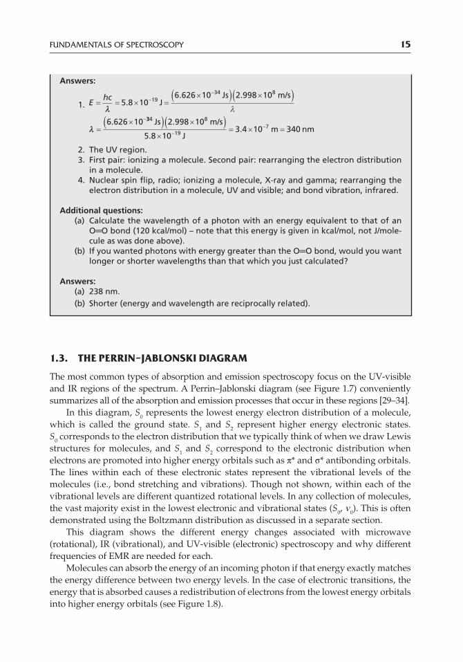
1.3. THE PERRIN–JABLONSKI DIAGRAM
The most common types of absorption and emission spectroscopy focus on the UV‐visible and IR regions of the spectrum. A Perrin–Jablonski diagram (see Figure 1.7) conveniently summarizes all of the absorption and emission processes that occur in these regions [29–34].
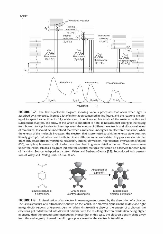
In this diagram, S0 represents the lowest energy electron distribution of a molecule, which is called the ground state. S1 and S2 represent higher energy electronic states. S0 corresponds to the electron distribution that we typically think of when we draw Lewis structures for molecules, and S1 and S2 correspond to the electronic distribution when electrons are promoted into higher energy orbitals such as π* and σ* antibonding orbitals. The lines within each of these electronic states represent the vibrational levels of the molecules (i.e., bond stretching and vibrations). Though not shown, within each of the vibrational levels are different quantized rotational levels. In any collection of molecules, the vast majority exist in the lowest electronic and vibrational states (S0, v0). This is often demonstrated using the Boltzmann distribution as discussed in a separate section.
This diagram shows the different energy changes associated with microwave ( rotational), IR (vibrational), and UV‐visible (electronic) spectroscopy and why different frequencies of EMR are needed for each.
Molecules can absorb the energy of an incoming photon if that energy exactly matches the energy difference between two energy levels. In the case of electronic transitions, the energy that is absorbed causes a redistribution of electrons from the lowest energy orbitals into higher energy orbitals (see Figure 1.8).
Answers:
1. Ehc
5 8 106 626 10 2 998 10
6 626 10
1934 8
.. .
.
JJs m/s
334 8
197
2 998 10
5 8 103 4 10 340
Js m/s
Jm nm
.
..
2. The UV region.3. First pair: ionizing a molecule. Second pair: rearranging the electron distribution
in a molecule.4. Nuclear spin flip, radio; ionizing a molecule, X‐ray and gamma; rearranging the
electron distribution in a molecule, UV and visible; and bond vibration, infrared.
Additional questions:(a) Calculate the wavelength of a photon with an energy equivalent to that of an
O═O bond (120 kcal/mol) – note that this energy is given in kcal/mol, not J/mole-cule as was done above).
(b) If you wanted photons with energy greater than the O═O bond, would you want longer or shorter wavelengths than that which you just calculated?
Answers:(a) 238 nm.(b) Shorter (energy and wavelength are reciprocally related).
0003959059.INDD 15 09/03/2018 8:17:02 AM
(S0 S1)(S0 S2)
(S1 S0)
(S2 S1)
(S1 S0)
(S1 T1)
(T1 S0)
(T1 S0)
S2
S0
S1
T1
vvvv
vvvv
vvvv
vvvv
Internal conversion
Intersystemcrossing
Internal conversion
Vibrational relaxation
ISC hυin hυin
hυout hυoutAbsorbance Absorbance
Fluorescence
Energy
Phosphorescence
Absorbance
Wavelength
Fluorescence Phosphorescence
S0 S2 S0 S1 S1 S0 T1 S0
FIGURE 1.7 The Perrin–Jablonski diagram showing various processes that occur when light is absorbed by a molecule. There is a lot of information contained in this figure, and the reader is encour-aged to spend some time to fully understand it as it underpins much of the material in this and subsequent chapters. The arrow at the far left is important to note. It indicates that energy is increasing from bottom to top. Horizontal lines represent the energy of different electronic and vibrational levels of molecules. It should be understood that when a molecule undergoes an electronic transition, while the energy of the molecule increases, the electron that is promoted to a higher energy state does not literally go “up”, but rather is redistributed into a different molecular orbital. Key processes in this dia-gram include absorption, vibrational relaxation, internal conversion, fluorescence, intersystem crossing (ISC), and phosphorescence, all of which are described in greater detail in the text. The curves shown under the Perrin–Jablonski diagram indicate the spectral features that could be observed for each type of transition. Source: Adapted in part from Valeur and Berberan‐Santos [28]. Reproduced with permis-sion of Wiley‐VCH Verlag BmbH & Co. KGaA.
N
N
O O
HH
Absorption ofa photon
Ground state electron distribution
Excited state electron distribution
Lewis structure of4-nitroaniline
FIGURE 1.8 A visualization of an electronic rearrangement caused by the absorption of a photon. The Lewis structure of 4‐nitroaniline is shown on the far left. The electron clouds in the middle and right image depict regions of electron density. When 4‐nitroaniline absorbs the energy of a photon, the electrons get redistributed into different orbitals, with the resulting electron distribution being higher in energy than the ground state distribution. Notice that in this case, the electron density shifts away from the amine group toward the nitro group as a result of the electronic transition.
0003959059.INDD 16 09/03/2018 8:17:03 AM
FUNDAMENTALS OF SPECTROSCOPY 17
For our discussion, we consider what happens when a molecule transitions from the ground state (S0/v0) into the fourth vibrational level of the second excited state (S2/v4). In order to go from S0/v0 to S2/v4, the molecule has to absorb the energy of a photon. So immediately upon absorption, the energy of the molecule increases by exactly the amount of energy the photon had. After being promoted to this new level, the molecule rapidly begins to shed the energy it absorbed. This process is called vibrational relaxation. Vibrational energy is lost through collisions between the excited state molecule and sur-rounding solvent molecules, with the energy being converted to a miniscule amount of increased kinetic energy of the solvent [35].
After relaxing to the lowest vibrational level within S2, most molecules undergo a process called internal conversion, which occurs when the lowest vibrational level of S2 overlaps with higher vibrational levels in S1. The energy within the molecule is redistrib-uted into a new electronic distribution and different vibrational modes. After this conversion from one excited state to another, additional vibrational relaxation within S1 occurs, and the molecule quickly relaxes into the ground vibrational level (v0) of S1 [35]. Several different processes can take place once an excited molecule is in this state: fluores-cence, external conversion, internal conversion, or intersystem crossing.
Fluorescence is the emission of a photon from a singlet excited state molecule, return-ing the molecule to the singlet ground state. “Singlet state” simply means that all electron spins are paired (one spin‐up for every one spin‐down). The emitted photon carries away the specific amount of energy required to return the molecule from the ground vibra-tional state in S1 back to any of the vibrational levels within S0. A few molecules also exhibit fluorescence directly from S2 to S0, but fluorescence from the S1 state is much more common [35].
External conversion is a radiationless relaxation process, meaning that no photon is emitted as the molecule loses energy to return to the ground state. It occurs through collisions of the excited state with surrounding solvent molecules, during which the sol-vent gains energy, while the excited molecule loses it, resulting in a very slight increase in the temperature of the solvent. Nonradiative decay also occurs via internal conversion from the ground vibrational state in S1 to a high vibrational state in S0 followed by vibra-tional relation.
Intersystem crossing involves the redistribution of the energy of the singlet S1 state into a triplet state, symbolized as T1 (see Figure 1.7). A triplet state is one in which all of the electrons in a molecule are paired except for two, which both have the same spin. The pro-cess of going from a singlet to a triplet state is known as a “spin‐forbidden transition.” While we use the term “forbidden,” in reality some molecules can undergo this process, but the probability of its occurrence is low. Once in the triplet state, molecules undergo vibrational relaxation to the lowest vibrational level. Molecules can then either relax to S0 via external conversion (i.e., radiationless collisional deactivation) or emit a photon with an energy that matches the energy difference between the lowest vibrational state in T1 and any of the vibrational states in S0. Again, this is a quantized transition in that only photons with specific energy matching the energy level gaps are emitted. Emission of this type is referred to as phosphorescence (see Figure 1.7). Like the S1 → T1 transition, the T1 → S0 transition is also spin forbidden and of low probability. This has implications about the timescale on which it occurs as discussed in the next section.
0003959059.INDD 17 09/03/2018 8:17:03 AM
18 SPECTROSCOPY
You have observed phosphorescence if you have seen glow‐in‐the‐dark stickers or bracelets. To activate them, they are exposed to light and the molecules absorb that light, promoting the molecules into excited states that ultimately transition into the excited triplet state. When the lights are turned off, you can see the light they emit as they return from the excited triplet state to the ground singlet state. Because this transition is also of low probability, it can take minutes or hours for all of the molecules to eventually return to the ground state, which is why the stickers and bracelets continue to glow even after the light is turned off. The intensity of the glow fades over time as more of the molecules return to the ground state, and fewer are left in the excited state.
1.3.1. Timescales of Events
Besides depicting the different energy scales involved in the various types of spectroscopy and the quantum transitions involved in each, the Perrin–Jablonski diagram also allows for a discussion of lifetimes of the molecules in the various states associated with the different processes (see Table 1.3 for the approximate timescales) [28].
Absorption occurs on a femtosecond (10−15 s) timescale. In this short period of time, the electrons are rearranged within the molecule, but the much more massive nuclei do not have time to move. The fact that the nuclei can be viewed as essentially motionless during absorption is known as the Franck–Condon principle and also relates to the Born–Oppenheimer approximation [36, 37].
Vibrational relaxation takes picoseconds to fractions of a nanosecond (10−12 to 10−10 s), during which time solvent molecules begin to reorient themselves to better interact with the new electronic distribution of the excited state molecule. Internal conversion also occurs on the picosecond timescale.
Fluorescing molecules typically remain in the lowest excited singlet state from 10−10 to 10−7 seconds before emitting a photon. If nonradiative processes occur faster, then little or no fluorescence is observed. Structural effects and thermal effects play a big role here. Most molecules are not fluorescent because they can lose energy through vibrations and rotations that transfer energy to other molecules. These nonradiative decay mechanisms decrease the likelihood of the molecule relaxing to the ground state via fluorescence. Structurally rigid molecules, however, like polyaromatic hydrocarbons with electron donating and accepting groups on them, tend to be fluorescent. This is simply because relaxation via fluorescence competes on the same timescale as nonradiative decay for
TABLE 1.3 Approximate Timescales for Processes Associated with Spectroscopy
Transition Timescale
Absorption 10−15 s (femtoseconds)Vibrational relaxation 10−12 to 10−10 s (picoseconds to subnanoseconds)Internal conversion 10−11 to 10−9 s (tens of picoseconds to nanoseconds)Fluorescence 10−10 to 10−7 s (subnano‐ to submicroseconds)Intersystem crossing 10−10 to 10−8 s (around a nanosecond)Phosphorescence 10−6 to 10 s (milliseconds to seconds)
Source: From Valeur and Berberan‐Santos [28]. Reproduced with permission of John Wiley & Sons.
0003959059.INDD 18 09/03/2018 8:17:03 AM
FUNDAMENTALS OF SPECTROSCOPY 19
these molecules. Similarly, fluorescence tends to increase as the temperature of a sample decreases because the molecules are moving more slowly, meaning they bump into one another less frequently and with less energy, thereby increasing their likelihood of fluorescing rather than undergoing nonradiative decay.
As noted above, phosphorescence is spin forbidden. It is therefore an unlikely process and takes a long time, with triplet state lifetimes ranging from milliseconds to minutes. Thus, phosphorescence, when it occurs, is a long‐lived phenomenon, as discussed above in the context of glow‐in‐the‐dark stickers and bracelets. As with fluorescence, colder tem-peratures reduce the nonradiative mechanism of relaxation, increasing the probability that an excited state molecule phosphoresces. It is for this reason that glow‐in‐the‐dark bracelets last longer if stored in a refrigerator or freezer after being exposed to the sun.
1.3.2. Summary of Radiative and Nonradiative Processes
The section above covered a lot of ground. It is an important section as it encapsulates much of modern spectroscopy. Absorption has to occur in order for fluorescence or phosphorescence to occur. Therefore, only molecules that tend to absorb a lot of radiation in the UV‐visible region are fluorescent or phosphorescent. There are many pathways by which molecules that have absorbed energy can relax back down to the ground state, with phosphorescence being the slowest and therefore least likely, as other relaxation events usually occur before phosphorescence does. Structure, solvent, and temperature all affect the likelihood of absorption, fluorescence, and phosphorescence. Temperature effects are discussed below, and the effects of the other factors are described in greater detail in subsequent chapters.
1.4. TEMPERATURE EFFECTS ON GROUND AND EXCITED STATE POPULATIONS
Virtually all spectroscopic techniques that are based on absorbance rely on the fact that the population of molecules in the ground state exceeds that in the excited state. The extent of this population difference depends on the energy gap between the ground and excited states and on the temperature. High temperatures mean that molecules have more energy, and this energy can be used to populate higher energy states. The ratio of molecules in a low energy state to that in a high energy state is given by the Boltzmann distribution:
NN
PP
eE
kT* * (1.8)
where N* and N° represent the number of atoms in a sample in the higher and lower states, respectively; P* and P° are statistical parameters related to the number of states of equivalent energy for the higher and lower states, respectively; ΔE is the difference in energy between the two states in Joules; T is the sample temperature in Kelvin; and k is the Boltzmann constant, 1.3806 × 10⁻²³ J/K. For atomic transitions such as for an s‐orbital → p‐orbital excitation, P° is 2, as there are two ways an electron can occupy a single s‐orbital (either spin‐up or spin‐down), and P* is 6 because there are three p‐orbitals, each with spin‐up/spin‐down possibilities, all of which are equivalent in energy.
0003959059.INDD 19 09/03/2018 8:17:03 AM
20 SPECTROSCOPY
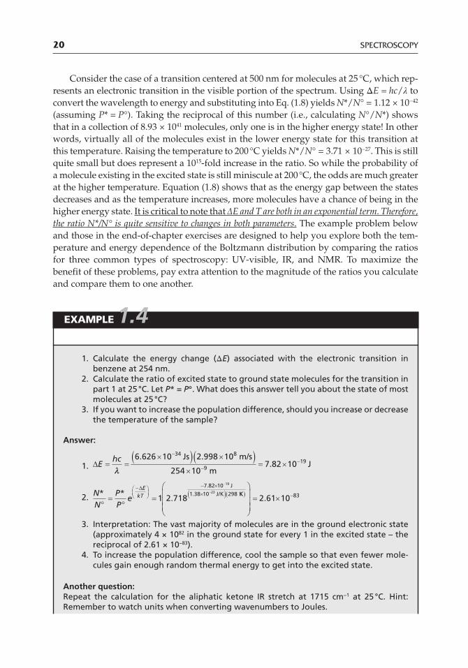
Consider the case of a transition centered at 500 nm for molecules at 25 °C, which rep-resents an electronic transition in the visible portion of the spectrum. Using ΔE = hc/λ to convert the wavelength to energy and substituting into Eq. (1.8) yields N*/N° = 1.12 × 10−42 (assuming P* = P°). Taking the reciprocal of this number (i.e., calculating N°/N*) shows that in a collection of 8.93 × 1041 molecules, only one is in the higher energy state! In other words, virtually all of the molecules exist in the lower energy state for this transition at this temperature. Raising the temperature to 200 °C yields N*/N° = 3.71 × 10⁻²⁷. This is still quite small but does represent a 1015‐fold increase in the ratio. So while the probability of a molecule existing in the excited state is still miniscule at 200 °C, the odds are much greater at the higher temperature. Equation (1.8) shows that as the energy gap between the states decreases and as the temperature increases, more molecules have a chance of being in the higher energy state. It is critical to note that ΔE and T are both in an exponential term. Therefore, the ratio N*/N° is quite sensitive to changes in both parameters. The example problem below and those in the end‐of‐chapter exercises are designed to help you explore both the tem-perature and energy dependence of the Boltzmann distribution by comparing the ratios for three common types of spectroscopy: UV‐visible, IR, and NMR. To maximize the benefit of these problems, pay extra attention to the magnitude of the ratios you calculate and compare them to one another.
1. Calculate the energy change (ΔE) associated with the electronic transition in benzene at 254 nm.
2. Calculate the ratio of excited state to ground state molecules for the transition in part 1 at 25 °C. Let P* = P°. What does this answer tell you about the state of most molecules at 25 °C?
3. If you want to increase the population difference, should you increase or decrease the temperature of the sample?
Answer:
1. Ehc 6 626 10 2 998 10
254 107 82 10
34 8
919
. ..
Js m/s
mJ
2. NN
PP
eE
kT* *.
.
. /1 2 718
7 82 10
1 38 10 298
19
23
J
J K KK2 61 10 83.
3. Interpretation: The vast majority of molecules are in the ground electronic state (approximately 4 × 1082 in the ground state for every 1 in the excited state – the reciprocal of 2.61 × 10−83).
4. To increase the population difference, cool the sample so that even fewer mole-cules gain enough random thermal energy to get into the excited state.
Another question:Repeat the calculation for the aliphatic ketone IR stretch at 1715 cm−1 at 25 °C. Hint: Remember to watch units when converting wavenumbers to Joules.
EXAMPLE 1.4
0003959059.INDD 20 09/03/2018 8:17:03 AM
FUNDAMENTALS OF SPECTROSCOPY 21
1.5. MORE WAVE CHARACTERISTICS
In the previous section we saw a range of effects that EMR has on atoms and molecules. To take advantage of these effects to measure chemical properties, we need to examine additional characteristics and processes associated with EMR.
1.5.1. Adding Waves Together
An electromagnetic wave propagating through space and time can be described using a sine function as shown in Eq. (1.9):
y A tsin 2 (1.9)
where y is the magnitude of the electric field, A is the maximum amplitude of the electric field, t is time, υ is the frequency of the EMR, and ϕ is the phase angle.
Two or more waves traveling through the same space add together to create one resulting wave as shown in Figure 1.9. When the individual waves reinforce one another and create a wave of greater amplitude, the waves are said to constructively interfere. In contrast, destructive interference occurs when two waves cancel each other. For perfect constructive interference, the two waves must have the same frequency and the same phase as one another. Perfect destructive interference occurs when the two waves have the same frequency and are 180° out of phase, as shown in Figure 1.10.
Adding together any number of waves results in a new wave that has its own unique periodicity or beat pattern as shown in Figure 1.9d. What is critical about this is that the reverse process is also true, meaning that any regularly repeating pattern can be decon-volved into the original component waves. This process, depicted in Figure 1.11, is known as Fourier transformation (FT) and lies at the heart of FTIR and FT‐NMR spectroscopy. In these techniques, a single signal is recorded in time, and the Fourier transformation is used to determine the frequencies and intensities of the EMR making up the signal. This information is translated into structural and quantitative information about the molecules in the sample.
1.5.2. Diffraction
Diffraction is a process that occurs when EMR propagating through space encounters obstacles, slits, or small holes that are roughly comparable in size to the wavelength of the radiation. It ultimately results from the interference phenomena described above.
Answer:
NN
*. .2 53 10 4
Interpretation: About 1 out of every 3950 molecules is in the excited vibrational state at this temperature, so most are still in the ground state, but this ratio is not nearly as skewed as that calculated above for a UV‐visible electronic transition. As above, cooling the sample further increases this difference.
0003959059.INDD 21 09/03/2018 8:17:04 AM
22 SPECTROSCOPY
Beams of light that travel different distances can constructively or destructively inter-fere depending on the exact difference in the path lengths and the wavelengths of the EMR. Consider the example in Figure 1.12 [38, 39] in which two beams of X‐rays are reflected off of two atoms separated by a distance, d, in a crystal. Assuming that the X‐rays are emitted by the same source, beam 2 travels an extra distance, ABC, compared to beam 1 before striking the detector surface. If the extra distance is a multiple of the wavelength of the light, then constructive interference occurs and the two beams reinforce one another. The requirement for the extra length traveled to be a multiple of the wavelength of the EMR can be likened to two people who start out marching in step with one another, each
–8
–4
0
4
8
0 20 40 60
–8
–4
0
4
8
0 20 40 60
–8
–4
0
4
8
0 20 40 60
–8
–4
0
4
8
(a)
(b)
(c)
(d)
0 20 40 60
FIGURE 1.9 Three waves (a, b, and c) added together to create a fourth wave (d). Note that each of the waves has a different frequency and amplitude. The amplitudes (y‐axis values) at each x‐axis value of the first three waves are added to yield the wave in (d). The sum (d) itself has a characteristic pattern. When the process is run in reverse, the single wave in (d) can be deconvolved to yield the frequencies and amplitudes of the three waves that constitute it. This is the basis of Fourier transforma-tion and is depicted in a subsequent figure.
0003959059.INDD 22 09/03/2018 8:17:04 AM
FUNDAMENTALS OF SPECTROSCOPY 23
covering 6 feet of ground for every left/right cycle. If one of the two walks an extra 6 feet, then they are still in step, and the same is true for 12, 18, 24 feet, etc. But if one of them only travels, say, 4 extra feet, then they would no longer be in stride with one another.
Referring back to Figure 1.12, it can be shown using rules of trigonometry that con-structive interference occurs when
n d2 sin (1.10)
where n is any integer (1, 2, 3, etc.), λ is the wavelength of the electromagnetic radiation, d is the spacing between layers of atoms, and θ is the angle of incidence and reflection.
You have likely already observed the effects of diffraction if you have looked at the back of a CD or DVD and seen the rainbow. The tiny pits on the back of CDs and DVDs that encode the information onto the discs diffract light. So when you look at the disc, you
–2
–1
0
1
2
–2
–1
0
1
2
–2
–1
0
1
2
–2
–1
0
1
2
–2
–1
0
1
2
–2
–1
0
1
2
Constructive interference(a) (b)
Destructive interference
FIGURE 1.10 An illustration of constructive and destructive interference. In both (a) and (b), the top two graphs are added together and create the bottom graph. So the graph on the bottom is the result of adding the y‐value of the top two graphs at every point along the x‐axis. So in (a), when both curves have a y‐value of 1.00 at the same x‐value, the result is a y‐value of 2.0 at the corresponding x‐value. In (b), which represents perfect destructive interference, the value of y in the top curve is always offset by the same value in the negative direction in the second curve. The result is zero amplitude at all x‐values.
0003959059.INDD 23 09/03/2018 8:17:05 AM
24 SPECTROSCOPY
–1.5
–0.5
0.5
1.5
–1
0
1
–4–2024
–1.5
–0.5
0.5
1.5
–8–4048
–8–4048
–3–1.5
01.5
3
–10
0
10
–20
–15
–10
–5
0
5
10
15
20
25
Sig
nal
Time
Fourier transformation
FIGURE 1.11 Depiction of the Fourier transformation during which a single complex signal versus time input (left) gets deconvolved into the constituent frequencies and their associated amplitudes that make up the signal (right). Note that the y‐axis scales (i.e., amplitudes) are different for the individual waves on the right. The frequency information contained in spectra provides clues about molecular structure (i.e., qualitative information), and the amplitude (i.e., intensity) provides quantitative information related to concentration.
1
2
3
Distance betweenlayers of atomsin crystal, d
Extra distance traveled by rays 2 and 3
θ θ
A
B
C
FIGURE 1.12 Schematic of diffraction of electromagnetic radiation from atoms in a crystal. Constructive interference occurs when the extra distance traveled by rays 2 and 3 is a multiple of the wavelength of incoming radiation. Source: Reproduced with kind permission of A. Vantomme, KU Leuven.
0003959059.INDD 24 09/03/2018 8:17:05 AM
FUNDAMENTALS OF SPECTROSCOPY 25
are seeing the white light that is broken into its constituent wavelengths. Different wavelengths of light (λ) are constructively reinforced at different angles (θ). This same phenomenon of diffraction is also the basis for components in spectrophotometers called diffraction gratings, which we discuss in more detail in Chapter 2.
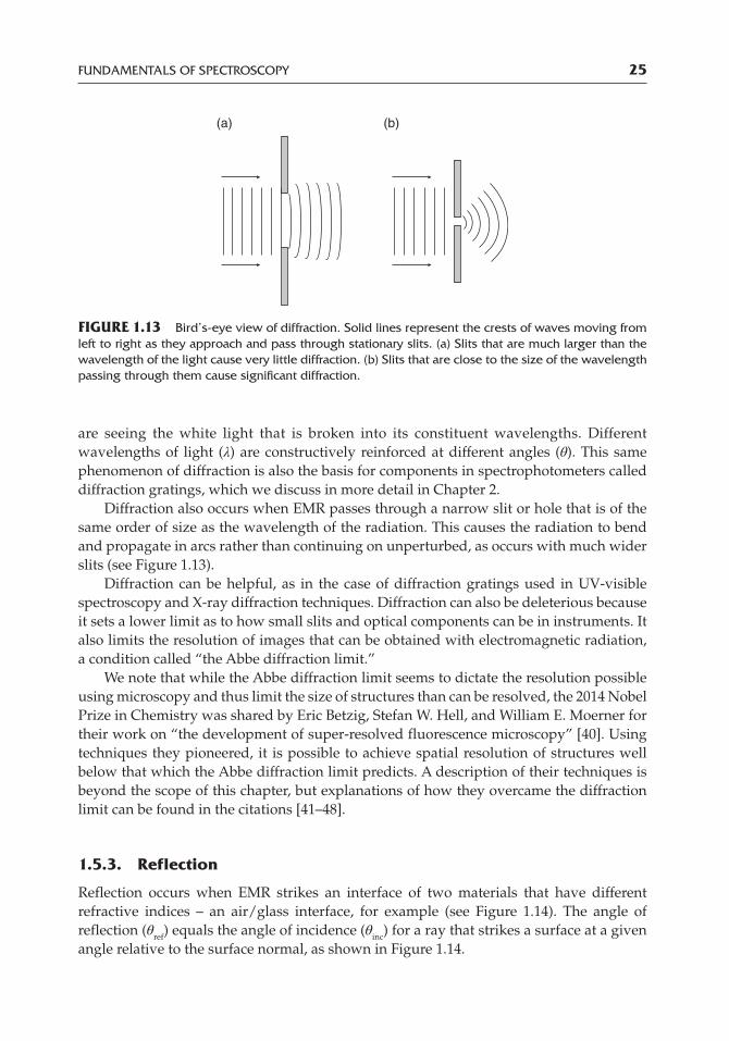
Diffraction also occurs when EMR passes through a narrow slit or hole that is of the same order of size as the wavelength of the radiation. This causes the radiation to bend and propagate in arcs rather than continuing on unperturbed, as occurs with much wider slits (see Figure 1.13).
Diffraction can be helpful, as in the case of diffraction gratings used in UV‐visible spectroscopy and X‐ray diffraction techniques. Diffraction can also be deleterious because it sets a lower limit as to how small slits and optical components can be in instruments. It also limits the resolution of images that can be obtained with electromagnetic radiation, a condition called “the Abbe diffraction limit.”
We note that while the Abbe diffraction limit seems to dictate the resolution possible using microscopy and thus limit the size of structures than can be resolved, the 2014 Nobel Prize in Chemistry was shared by Eric Betzig, Stefan W. Hell, and William E. Moerner for their work on “the development of super‐resolved fluorescence microscopy” [40]. Using techniques they pioneered, it is possible to achieve spatial resolution of structures well below that which the Abbe diffraction limit predicts. A description of their techniques is beyond the scope of this chapter, but explanations of how they overcame the diffraction limit can be found in the citations [41–48].
1.5.3. Reflection
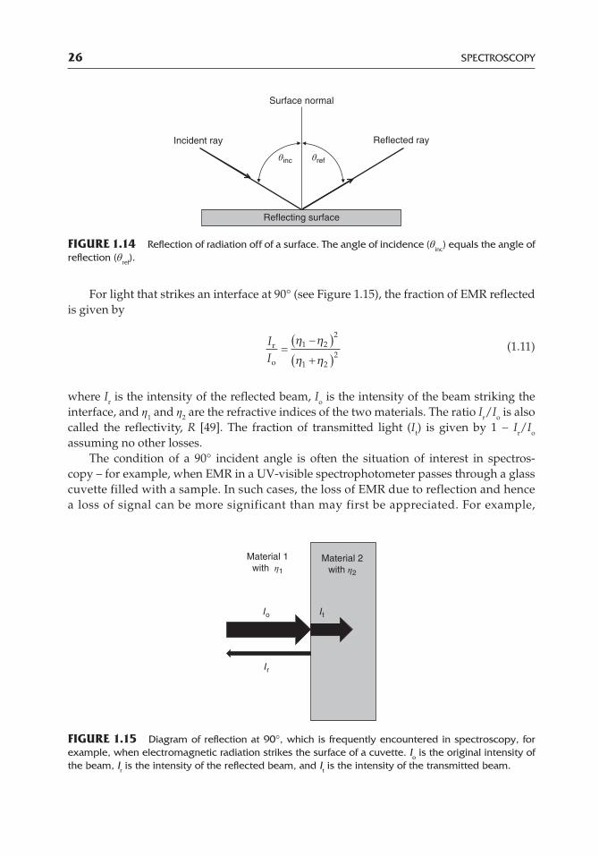
Reflection occurs when EMR strikes an interface of two materials that have different refractive indices – an air/glass interface, for example (see Figure 1.14). The angle of reflection (θref) equals the angle of incidence (θinc) for a ray that strikes a surface at a given angle relative to the surface normal, as shown in Figure 1.14.
(b)(a)
FIGURE 1.13 Bird’s‐eye view of diffraction. Solid lines represent the crests of waves moving from left to right as they approach and pass through stationary slits. (a) Slits that are much larger than the wavelength of the light cause very little diffraction. (b) Slits that are close to the size of the wavelength passing through them cause significant diffraction.
0003959059.INDD 25 09/03/2018 8:17:06 AM
26 SPECTROSCOPY
For light that strikes an interface at 90° (see Figure 1.15), the fraction of EMR reflected is given by
II
r
o
1 22
1 22
(1.11)
where Ir is the intensity of the reflected beam, Io is the intensity of the beam striking the interface, and η1 and η2 are the refractive indices of the two materials. The ratio Ir/Io is also called the reflectivity, R [49]. The fraction of transmitted light (It) is given by 1 − Ir/Io assuming no other losses.
The condition of a 90° incident angle is often the situation of interest in spectros-copy – for example, when EMR in a UV‐visible spectrophotometer passes through a glass cuvette filled with a sample. In such cases, the loss of EMR due to reflection and hence a loss of signal can be more significant than may first be appreciated. For example,
Reflecting surface
θinc θref
Surface normal
Incident ray Reflected ray
FIGURE 1.14 Reflection of radiation off of a surface. The angle of incidence (θinc
) equals the angle of reflection (θ
ref).
Io
Ir
It
Material 2with η2
Material 1with η1
FIGURE 1.15 Diagram of reflection at 90°, which is frequently encountered in spectroscopy, for example, when electromagnetic radiation strikes the surface of a cuvette. I
o is the original intensity of
the beam, Ir is the intensity of the reflected beam, and I
t is the intensity of the transmitted beam.
0003959059.INDD 26 09/03/2018 8:17:06 AM
FUNDAMENTALS OF SPECTROSCOPY 27
as shown in Figure 1.16, EMR passing through a filled cuvette encounters four interfaces, with EMR being reflected at each one, such that the intensity being passed on to interface 2 is less than that which strikes interface 1, and that striking interface 4 is less than that at 3, 2, and 1. As you will see when performing the calculation in Example 1.5, the beam that eventually emerges from the cuvette has been reduced in strength by nearly 10%. Keep in mind that in optical systems, many such interfaces can exist with the concomitant reduction in the intensity of the beam. For this reason, many instrument designs try to minimize the number of interfaces in order to maximize the throughput of electromagnetic radiation.
Equation (1.11) shows that the percent of reflected radiation increases as the difference in the refractive indices of the two materials creating the interface increases. It also shows that when the two materials have identical refractive indices (i.e., η1 = η2), no EMR is reflected and it all passes through the interface. For this reason, in some applications optical components are bathed in liquids that have refractive indices that match that of glass or the sample to reduce reflections [50, 51]. This is known as refractive index match-ing and is used in applications where minimizing the loss of EMR, and hence the loss of signal, is required.
???photons
10 000photons
FIGURE 1.16 Diagram of light from a source passing through a quartz cell filled with an aqueous sample.
1. In a typical UV‐visible experiment, an aqueous sample is contained in a quartz cuvette. Assuming 10 000 photons strike the surface of the cuvette, calculate how many actually make it through the cuvette and the sample and emerge out the other side.
2. What percentage is this? Assume that the sample is aqueous, that the light is striking at a 90° angle at each interface, and that the refractive index of air is 1.00. Use the table presented earlier in this chapter to find refractive indices, assuming that the refractive index of an aqueous solution is equal to that of water.
Answer:The diagram in Figure 1.16 shows that there are four interfaces to consider when answering the question: air/quartz, quartz/water, water/quartz, and quartz/air.
EXAMPLE 1.5
0003959059.INDD 27 09/03/2018 8:17:06 AM
28 SPECTROSCOPY
1.5.4. Refraction
Refraction is the apparent bending of a beam of EMR as it propagates through an interface at an angle. The extent of refraction depends on the angle at which the radiation enters the interface and on the refractive indices of the materials that comprise it. The effect is depicted in Figure 1.17, and the angle to which the beam is bent is given by Snell’s law, shown in Eq. (1.12):
sinsin
1
2
2
1
(1.12)
where θ1 and θ2 are the angles at which the radiation enters and leaves the interface, respectively, both relative to the normal of the interface as shown in the figure and where η1 and η2 are the refractive indices of the two materials.
The effect ultimately arises from the fact that the velocity of the EMR is slower in the material with the higher refractive index. The bending of the beam mimics a marching band pivoting to turn a corner [52, 53]. The person on one end must slow down or essen-tially march in place, while the person on the other end must continue to march rapidly in order to maintain formation while turning the corner. Similarly, the first rays of a beam that enter the higher refractive index material slow down, while the part of the beam that has yet to encounter the interface continues to travel more rapidly until it too encounters the interface and slows down, at which point all parts of the beam are proceeding with the same velocity through the second medium. We commonly observe this effect when objects such as straws or plant stems appear to be bent when placed in a glass or vase filled with water.
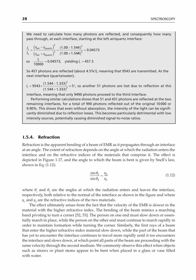
We need to calculate how many photons are reflected, and consequently how many pass through, at each interface, starting at the left air/quartz interface:
IIr
o
air quartz
air quartz
2
2
21 00 1 544
1 00 1 54
. .
. . 440 04573
100000 04573 457 3
2 .
. , .so yieldingrr
II
So 457 photons are reflected (about 4.5%!), meaning that 9543 are transmitted. At the next interface (quartz/water),
Ir 95431 544 1 333
1 544 1 33351
2
2
. .
. ., so another 51 photons are lost due to reflection at this
interface, meaning that only 9490 photons proceed to the third interface.Performing similar calculations shows that 51 and 431 photons are reflected at the two
remaining interfaces, for a total of 990 photons reflected out of the original 10 000 or 9.90%. This shows that even without absorption, the intensity of the light can be signifi-cantly diminished due to reflection losses. This becomes particularly detrimental with low intensity sources, potentially causing diminished signal‐to‐noise ratios.
0003959059.INDD 28 09/03/2018 8:17:07 AM
FUNDAMENTALS OF SPECTROSCOPY 29
1.5.5. Scattering
In addition to the above phenomena of diffraction, reflection, and refraction, when EMR interacts with matter, it can also be scattered. This occurs in several ways, including Rayleigh and Raman scattering and through the Tyndall effect.
1.5.5.1. Rayleigh Scattering. Rayleigh scattering is scattering of EMR due to mol-ecules that are much smaller than the wavelength of radiation being scattered. As EMR interacts with a molecule, like N2 or O2, the oscillating electric field of the radiation dis-torts the electron cloud of the molecule and causes the electrons to oscillate at the same frequency as the radiation. The oscillating electrons then radiate electromagnetic radiation [54]. The wavelength of this scattered radiation is the same as that which induced the elec-tron oscillation. In other words, Rayleigh scattering is an elastic process, meaning that the energy of the scattered photons is the same as that of the incoming photons. The scattering occurs in all directions, but the intensity depends on the angle at which the scattering is being observed.
The intensity of Rayleigh scattering is given by [55]
II N
r
o 8 14 2 2
4 2
cos (1.13)
where Io is the intensity of the light striking the scatterers, α is the polarizability of the scat-terers, N is the number of scatterers per cm3, θ is the angle of the scattered radiation, r is the distance between the scatterers and the observer, and λ is the wavelength of the scat-tered radiation. Notice that the intensity of scattering depends on 1/λ4. Thus, there is a strong dependence on the wavelength of light. This, in fact, is why the sky is blue. The sun essentially emits all wavelengths of visible light. The beams encounter particles that scatter the light as they propagate through space. Blue light, having the smallest wave-lengths, is scattered the most, and it is scattered at all angles, so when we look at areas of the sky away from the sun, they appear blue. When we look directly at the sun, it appears
θ1
θ2
Medium 1with η1
Ray
Wavefront
Medium 2with η2
FIGURE 1.17 Refraction of a beam of light as it transitions from one medium to another, such as the transition from air to water. The degree to which the beam is bent is given by Snell’s law and depends on the refractive indices of the two media. In this diagram, η
1 < η
2.
0003959059.INDD 29 09/03/2018 8:17:07 AM
30 SPECTROSCOPY
yellow because the red, orange, and yellow light is scattered less and therefore reaches our eyes, whereas the blues, greens, and violets are removed by the scattering. One might think that the sun should look red because these wavelengths are least scattered, but there are visual perception and intensity issues regarding the sun’s output at different wave-lengths that ultimately make it appear yellow during the day. The sun does appear to be orange or red at sunrise and sunset, especially when there are a lot of particles in the sky from forest fires, volcanic eruptions, or pollution, because at sunrise and sunset the light from the sun must travel through more of the atmosphere, and thus it encounters more scattering particles, causing additional scattering of even some of the orange and yellow light relative to when the sun is directly above us at noon (see Figure 1.18). This additional scattering leaves only the orange and red wavelengths behind when we look directly at the sun (i.e., θ = 0).
Rayleigh scattering is also responsible for the line in America the Beautiful about “purple mountain majesty.” When we look at distant objects, like mountains, our eyes see the blue scattered radiation from the sky, which veils the object. The further away the object is, the more blue radiation is between us and the object, so distant mountains appear bluish or purplish. Artists are aware of this fact and paint objects that they want to seem far away in their scenes with a blue or purple hue – a technique known as “atmospheric perspective” or “aerial perspective.” Paintings such as Leonardo da Vinci’s Mona Lisa and Albert Bierstadt’s Looking up the Yosemite Valley are examples of works where atmospheric perspective is used.
Noon
Sunset
Afternoon
Earth’satmosphere
Earth
CB
A
FIGURE 1.18 Rayleigh scattering creates red sunsets because the light from the sun has to travel further through the atmosphere at sunset than at noon, as seen by comparing the distance labeled “A” (sunset) to the one labeled “C” (noon). At noon, the light passes through the least amount of atmosphere and thus encounters the fewest number of scattering particles. In this case, it is mostly the short wave-length blue light that is scattered. Light with intermediate wavelengths associated with orange, yellow, and green are not scattered much and the result is that the sun looks yellow when we look directly at it, while the sky looks blue due to it having been scattered at all angles by the atmosphere. The light at sunset travels through more atmosphere and thus encounters more scattering particles. Because of the extended path, yellows and greens also get scattered to some extent, creating the reddish orange colors in the sky around the sun that we are accustomed to seeing at sunset.
0003959059.INDD 30 09/03/2018 8:17:08 AM
FUNDAMENTALS OF SPECTROSCOPY 31
1.5.5.2. Tyndall Effect/Mie Scattering. The Tyndall effect refers to scattering that occurs off of larger particles (approximately 10% of the wavelength of light striking the particle). A common instance of this is a red laser beam propagating through a beaker of water. If we try to observe the beam from above the beaker (i.e., bird’s‐eye view) and the water is completely free of particles, we do not see it because none of the light is reflected toward our eyes. When colloidal particles are added to the water (imagine very dilute milk that has globules of protein and fat in it), the beam can be seen going through the solution. We are really seeing the part of the beam that has been scattered by the particles. The amount of radiation scattered varies with the size of the scatterers. Thus, this kind of scattering, which is also known as Mie scattering [56], is used to measure the size of polymers, large biomolecules, and colloids. It is also responsible for the fact that clouds appear white due to the scattering of radiation off of water droplets. As in Rayleigh scattering, the frequency of the scattered radiation is the same as that which originally interacted with the particles. Only its direction of propagation has changed.
1.5.5.3. Raman Scattering. In Raman scattering, unlike Rayleigh and Mie scattering, the frequency of the scattered radiation is different than that of the incoming radiation. This effect arises when a molecule in a given vibrational state (say, vo) temporarily absorbs a photon and subsequently reemits it at a different frequency as it relaxes to a different vibrational level than where it started. Two possibilities are depicted in Figure 1.19. In one, the molecule ultimately ends up in a higher vibrational level by emitting a photon of lower energy (longer wavelength) than the original photon. This is called a Stokes shift. In the other, the molecule ends up in a lower vibrational level by emitting a higher energy (shorter wavelength) photon than the original. This is called an anti‐Stokes shift. The first situation is much more probable as more molecules are in the lowest vibrational level when the radiation encounters them as was shown in the example problems related to the Boltzmann distribution. Raman spectroscopy has grown to be an important analytical technique and is discussed in much more detail in Chapter 5.
1.5.6. Polarized Radiation
Thus far we have considered nonpolarized electromagnetic radiation, or radiation in which the electric fields of the waves are tilted along any plane centered on the beam path. Figure 1.20 [57] shows four such beams, though more waves at other angles are certainly possible. If we take the perspective of viewing the electric field vectors of the beam com-ing directly at us, it can be depicted as shown in Figure 1.21a, where again only a limited number of all the possible angles are shown. For any individual wave, however, the electric field vector at any moment can be deconvolved into x‐ and y‐components as shown in Figure 1.21b.
To create polarized radiation, a beam of nonpolarized radiation is passed through a crystal or polarizing filter that selectively removes one component of the radiation. If the x‐component is selectively removed, then the beam that emerges from the material is polarized along the y‐axis. In the case of complete removal of one component over the other, the radiation is referred to as linearly polarized or plane polarized radiation because the resulting electric component oscillates in a single plane.
0003959059.INDD 31 09/03/2018 8:17:08 AM
32 SPECTROSCOPY
Ground vibrational state, v = 0
First vibrational excited state, v = 1
Energy
hυin
hυin
hυout
hυout
Virtual state
Virtual state
Stokes shifthυout < hυin
Anti-Stokes shifthυout > hυin
FIGURE 1.19 Depiction of Raman scattering. As with the Perrin–Jablonski diagram, the increasing energy scale from bottom to top is important. Raman scattering involves the temporary uptake of a photon with some energy, and the subsequent reemission of a photon or either lower (Stokes) or higher (anti‐Stokes) energy. The former leaves the molecule in a higher vibrational state than it was in prior to absorbing the incoming radiation, and the latter results in the molecule being in a lower vibra-tional state after emission. In Raman scattering, unlike Rayleigh scattering, the energy of the emitted radiation is different than that of the incoming radiation, and therefore also has a different frequency and wavelength because E = h = hc/λ.
FIGURE 1.20 An illustration of multiple electromagnetic waves propagating through space, each oriented at a different angle relative to one another. Unpolarized light such as this has electric and magnetic components in planes at all angles. Source: Adapted from https://en.wikipedia.org/wiki/File:Wire‐grid‐polarizer.svg under GNU Free Documentation License. Created by B. Mellish for the English Wikipedia.
0003959059.INDD 32 09/03/2018 8:17:08 AM
FUNDAMENTALS OF SPECTROSCOPY 33
Circularly polarized radiation can also be created. In this case, the resultant electric field vector continuously rotates clockwise or counterclockwise as depicted in Figure 1.22 such that when viewed end on as if the beam were propagating straight at you, the resul-tant electric field vector appears to rotate in a circle as it comes toward you [58]. Some very helpful diagrams, animations, and videos can be found by searching the terms “linearly polarized light” and “circularly polarized light” on the Internet.
Plane polarized and circularly polarized EMR are used in many areas of spectroscopy. For example, the r‐ and s‐forms of stereoisomers absorb left and right circularly polarized
x
y
y-component
x-component
Electric field
(b)(a)
FIGURE 1.21 (a) A view of a few of the electric field components of unpolarized radiation propa-gating directly at the viewer. Note that the distribution would be random in all directions around the axis of propagation and varying in amplitude over time for each individual wave. (b) An individual electric field vector broken into x‐ and y‐components. The same deconstruction into x‐ and y‐compo-nents can be done for all of the waves in part (a).
FIGURE 1.22 Depiction of circularly polarized light. The electric field vector (arrows) rotates around the axis as it propagates through space in the direction indicated by the arrow on the right. Source: https://en.wikipedia.org/wiki/Circular_polarization. Licenced under CC BY SA 3.0.
0003959059.INDD 33 09/03/2018 8:17:09 AM
34 SPECTROSCOPY
radiation differently from one another, so circularly polarized light can be used to mea-sure the enantiomeric excess of one form of a molecule over another using a technique known as circular dichroism spectroscopy. Secondary structures like alpha helices and beta sheets in biomolecules like proteins and nucleic acids also impart a differential absorption of left‐ and right‐handed circularly polarized radiation. Therefore, circular dichroism spectroscopy is also used to study the structures of biomolecules and how they change with temperature, pH, and other environmental variables.
1.6. SPECTROSCOPY APPLICATIONS
Spectroscopy is one of the most universal and important analytical methods, and as we have indicated throughout this chapter, a wide range of applications exist. For example, NMR and IR spectroscopy are used to determine the structures of molecules. They can also be used in a quantitative manner to determine the concentration of specific substances in mixtures. UV‐visible spectroscopy is also commonly used for quantitative analyses. Techniques based on X‐ray spectroscopy are used to determine crystal structures and the elemental composition of a wide range of substances. In all of these instrumental methods of analysis, the properties of electromagnetic radiation, how it propagates through space, how it interacts with matter, and the effects it has on matter are important. Specific exam-ples of spectroscopic applications and how they take advantage of the interaction of electromagnetic radiation with matter are described in detail in the following chapters.
1.7. SUMMARY
In this chapter, we focused on the fact that molecules can absorb, reflect, refract, polarize, and scatter electromagnetic radiation. Measurements of these effects underlie a variety of spectroscopic techniques that yield qualitative and quantitative information about atoms and molecules. The next several chapters focus on specific types of spectroscopy, because each different wavelength range of the spectrum dictates instrument design, data collec-tion methods, and the analysis of results that are particular to each mode.
PROBLEMS
1.1 (a) When is it most helpful to think of electromagnetic radiation as a wave? (b) As a particle?
1.2 (a) Calculate the energy of a single photon with a frequency of 1.73 × 10¹⁷ Hz. (b) Calculate the wavelength and wavenumber of the photon in part (a). (c) What physical effects could such a photon cause in a molecule or atom? (d) Calculate the energy of a mole of these photons.
1.3 Calculate the wavelength of photons having 100.0 kcal/mol of energy (the approxi-mate energy of a mole of C─H bonds). Watch units carefully. What region of the electromagnetic spectrum is this in?
1.4 Consider two photons, one in the visible region of the spectrum with a 700.0 nm wavelength corresponding to red light and the other in the microwave region with a
0003959059.INDD 34 09/03/2018 8:17:09 AM
FUNDAMENTALS OF SPECTROSCOPY 35
wavelength of 2.000 × 10⁻² m. How many times more energetic is the red photon compared to the microwave photon?
1.5 The speed of 516.6 nm light (green light) in germanium is 6.503 × 10⁷ m/s (http://www.filmetrics.com/refractive‐index‐database/Ge/Germanium). What is the refractive index of germanium at this wavelength?
1.6 Calculate the refractive index of a Bose–Einstein condensate in which the speed of light was found to be 38 miles per hour.
1.7 Why do molecules typically fluoresce from the lowest energy vibrational state of the lowest energy excited state and not from higher energy states?
1.8 What is the difference between fluorescence and phosphorescence?
1.9 (a) NMR spectroscopy probes the difference between spin‐up (lower energy) and spin‐down states (higher energy) of nuclei in a magnetic field. Common NMR spectrometers operate around 400.0 MHz. Convert this frequency into an energy and then calculate the ratio of spin‐up to spin‐down states using the Boltzmann distribution equation at 25 °C. Let P* = P°.
(b) What does your answer tell you about the population difference of these two states?
1.10 Complete the table below. For simplicity, assume P* = P°.
Type Typical radiation
Temperature (°C) N*N°
N*/N°
N*/N°
UV‐visible 400 nm 25300
IR 1600 cm−1 25300
NMR 400 MHz 25300
1.11 This problem is designed to use the Boltzmann distribution to provide another way to compare the relative magnitudes of energy in the various regions of the spec-trum. This will be done through a critical comparison of the UV‐vis, IR, and NMR regions by calculating Boltzmann distribution ratios: (a) Calculate (N*/N°)NMR/(N*/N°)UV‐vis (i.e., calculate the ratio of the ratios) at 25 °C using values you calcu-lated in Problem 1.10, (b) Calculate (N*/N°)NMR/(N*/N°)IR at 25 °C using values you calculated in Problem 1.10. (c) Why is the ratio of N*/N° so much larger for NMR than it is for UV‐vis and IR spectroscopy?
1.12 (a) What wavelength of light produces constructive interference at a 30° angle when impinging on atoms separated by 1.5 Å (a typical C─C bond distance) assuming first order diffraction?
(b) At a 45° angle? (c) What region of the spectrum are these in?
1.13 What percent of electromagnetic radiation is reflected at a benzene/diamond inter-face assuming that the EMR is striking the interface at a 90° angle?
0003959059.INDD 35 09/03/2018 8:17:09 AM
36 SPECTROSCOPY
1.14 Which interface will produce more reflected light, water/heptane or water/benzene?
1.15 Consider radiation entering a water/diiodomethane interface at a 10° angle normal to the interface. At what angle will the radiation leave the interface?
1.16 What type of scattering occurs off of molecules that are much smaller than the wavelength of radiation being scattered?
1.17 What kind of scattering is used to measure the size of polymers and larger molecular clusters?
REFERENCES
1. Willard, H.H., Merritt, L.L. Jr., Dean, J.A., and Settle, F.A. Jr. (1988). Instrumental Methods of Analysis, 7e, 99. Belmont: Wadsworth Publishing Co.
2. Williamson, S.J. and Cummins, H.Z. (1983). Light and Color in Nature and Art, 180. New York: Wiley.
3. Pavia, D.L., Lampman, G.M., Kriz, G.S., and Engle, R.G. (2005). Introduction to Organic Laboratory Techniques: A Small Scale Approach, 2e. Salt Lake City: Brooks Cole Publishing Co.
4. Choi, M., Lee, S.H., Kim, Y. et al. (2011). Nature 470: 369–373.
5. http://www.engineeringtoolbox.com/refractive‐index‐d_1264.html (accessed 2 August 2017).
6. Haynes, W.M. (ed.‐in‐chief); Lide, D.R. and Bruno, T.J. (assoc. eds.) (2014). CRC Handbook of Chemistry and Physics, 95e. Boca Raton: CRC Press.
7. Riddick, J.A., Bunger, W.B., and Sakano, T.K. (1986). Organic Solvents: Physical Properties and Methods of Purification, Techniques of Chemistry, 4e, vol. II. New York: Wiley.
8. http://news.harvard.edu/gazette/1999/02.18/light.html (accessed 2 August 2017).
9. Pavia, D.L., Lampman, G.M., and Kriz, G.S. (2001). Introduction to Spectroscopy, 3e, 360. Pacific Grove: Brooks/Cole.
10. International Standard (2007). Space environment (natural and artificial) – process for determining solar irradiances. ISO 21348.
11. http://www.spacewx.com/pdf/SET_21348_2004.pdf (accessed 3 August 2017).
12. https://science.nasa.gov/ems/05_radiowaves (accessed 3 August 2017).
13. http://www.livescience.com/50399‐radio‐waves.html (accessed 3 August 2017).
14. Williams, P. and Norris, K. (eds.) (2001). Near‐infrared Technology: In the Agricultural and Food Industries, 2e. St. Paul: American Association of Cereal Chemists.
49. Strobel, H.A. and Heineman, W.R. (1989). Chemical Instrumentation: A Systematic Approach, 3e, 205. New York: Wiley.
50. Barcelo, D. (2005). Comprehensive Analytical Chemistry, volume 45, Analysis and Detection by Capillary Electrophoresis (ed. M.L. Marina, A. Rios and M. Valcarcel), 343. Amsterdam: Elsevier.
51. Poole, C.F. (2003). The Essence of Chromatography, 699. Amsterdam: Elsevier.
52. Donnelly, J. and Massa, N. (2007). Light: Introduction to Optics and Photonics. Boston: The New England Board of Higher Education.
53. DeValois, K.K. (2000). Seeing. New York: Academic Press.
55. Perkampus, H.H. (1993). Encyclopedia of Spectroscopy (trans. H.C. Grinter and R. Grinter), 508. Weinheim: Wiley‐VCH.
56. Parker, S.P. (ed.‐in‐chief) (1987). Optics Source Book, 223–224. New York: McGraw‐Hill Book Company.
57. https://en.wikipedia.org/wiki/File:Wire‐grid‐polarizer.svg (accessed 3 August 2017).
58. https://en.wikipedia.org/wiki/Circular_polarization (accessed 3 August 2017).
FURTHER READING
1. Avram, M. and Mateescu, G.D. (1970). Infrared Spectroscopy: Applications in Organic Chemistry (trans. L. Birladeanu). New York: Wiley.
2. Colthrup, N.B., Daly, L.H., and Wiberley, S.E. (1990). Introduction to Infrared and Raman Spectroscopy, 3e. San Diego: Academic Press, Inc.
3. Hercules, D. (ed.) (1966). Fluorescence and Phosphorescence Analysis: Principles and Applications. New York: Wiley.
4. Hollas, J.M. (2004). Modern Spectroscopy, 4e. Chichester: Wiley.
5. Ingle, J.D. Jr. and Crouch, S.R. (1988). Spectrochemical Analysis. Englewood Cliffs: Prentice Hall, Inc.
6. Jaffe, H.H. and Orchin, M. (1962). Theory and Applications of Ultraviolet Spectroscopy. New York: Wiley.
7. Lakowicz, J.R. (2006). Principles of Fluorescence Spectroscopy, 3e. New York: Springer.
8. Parker, S.P. (ed.‐in‐chief) (1987). Optics Source Book. New York: McGraw‐Hill Book Company.
9. Pavia, D.L., Lampman, G.M., and Kriz, G.S. (2008). Introduction to Spectroscopy, 4e. Pacific Grove: Brooks/Cole.
10. Perkampus, H.H. (1993). Encyclopedia of Spectroscopy (trans. H.C. Grinter and R. Grinter). Weinheim: Wiley‐VCH.
11. Rao, C.N.R. (1967). Ultra‐Violet and Visible Spectroscopy: Chemical Applications. New York: Plenum Press.
12. Smith, E. and Dent, G. (2005). Modern Raman Spectroscopy: A Practical Approach. Chichester: Wiley.
13. Tasumi, M. and Sakamoto, A. (eds.) (2015). Introduction to Experimental Infrared Spectroscopy: Fundamentals and Practical Methods. Chichester: Wiley.
14. Valeur, B. and Berberan‐Santos, M.N. (2013). Molecular Fluorescence: Principles and Applications, 2e. Weinheim: Wiley‐VCH.
15. Williamson, S.J. and Cummins, H.Z. (1983). Light and Color in Nature and Art. New York: Wiley.