Funding Value Adjustment and Valuing Interest Rate Swaps Msc Thesis Financial Econometrics Author: Hidde Schwietert Supervisor: Cees Diks Friday 26 th September, 2014 Abstract This thesis deals with the incorporation of both credit and funding risk in derivative valuation. The focus is on interest rate swaps for which an innovative framework is provided for modelling funding value adjustment (FVA) along with bilateral credit value adjustment (BCVA). In doing so, a case study is examined where a bank and a corporate enter into a plain vanilla interest rate swap. Underlying risk factors such as interest rates and credit spreads are modelled by stochastic processes while FVA is evaluated according to a Monte Carlo integration. In addition, we analyse the impact of wrong-way risk, credit spread levels and credit spread volatilities on FVA. FVA is find to have significant impact on derivatives valuation. Besides, FVA is found to be quite sensitive to changes in credit spread levels and volatilities. Hence, it is important to model thoroughly such dynamic features. Keywords: Counterparty Credit Risk, Funding Risk, Bilateral Credit Value Adjustment, Funding Value Adjustment, Interest Rate Swaps.
Transcript
Funding Value Adjustment and Valuing Interest Rate
Swaps
Msc Thesis Financial Econometrics
Author: Hidde SchwietertSupervisor: Cees Diks
Friday 26th September, 2014
Abstract
This thesis deals with the incorporation of both credit and funding risk in derivativevaluation. The focus is on interest rate swaps for which an innovative framework isprovided for modelling funding value adjustment (FVA) along with bilateral credit valueadjustment (BCVA). In doing so, a case study is examined where a bank and a corporateenter into a plain vanilla interest rate swap. Underlying risk factors such as interest ratesand credit spreads are modelled by stochastic processes while FVA is evaluated accordingto a Monte Carlo integration. In addition, we analyse the impact of wrong-way risk,credit spread levels and credit spread volatilities on FVA. FVA is find to have significantimpact on derivatives valuation. Besides, FVA is found to be quite sensitive to changesin credit spread levels and volatilities. Hence, it is important to model thoroughly suchdynamic features.
This thesis is the result of a graduation internship at Deloitte Financial Risk Management and rep-resents the completion of my MSc Financial Econometrics at the University of Amsterdam. First ofall, I gratefully acknowlegde the support of my supervisors prof. dr. Cees Diks (University of Ams-terdam) and Bastiaan Verhoef (Deloitte). Without their expertise, proper guidance and legitimateremarks I would not have been able to achieve this result. Furthermore, I would like to thank MichielLodewijk for the helpful discussions and steady encouragement along the project. Consequently, Iwould like to express my sincere gratitude to Deloitte for giving me the opportunity to do an in-ternship. Moreover, I am thankful to all my colleagues for supporting me throughout my internshipperiod. Special thanks go to Melissa Faizurachmi for her initial guidance, Martijn Westra for helpingme with some of my programming issues and Bas Hendriks for the calibration collaboration.
The global credit crisis resulted in regulatory and accounting changes regarding derivative valuation.
In January 2013, International Financial Reporting Standards 13 became effective, forcing banks and
other derivative dealers to incorporate credit value adjustment (CVA) and debt value adjustment
(DVA) in their fair derivative valuations. While the incorporation of CVA and DVA has been widely
studied and accepted by both practitioners and academics, the focus is now on the calculation and
relevance of funding value adjustment (FVA). The occurrence of FVA is highly linked with the
financial crisis. Prior to the crisis, LIBOR was often regarded as a suitable proxy for the risk-free
rate. Hence, collateral rates were commonly LIBOR based (Hull & White, 2013) and so funding
costs were offset. Through this, there was no need for a FVA. However, post crisis banks’ are not
considered as default free any more, hence the overnight indexed swap rate (OIS rate) has become
benchmark for risk-free rates. As a result, collateral rates have become mostly OIS based. Thus, as
funding has become relatively more costly and the interest received on collateral no longer offsets
the funding cost, the FVA has become non-negligible. Reflecting funding cost into the valuation of
derivatives has become a paramount topic in the financial industry. And yet, the literature is still
limited. At the moment there is no standard procedure involving both counterparty credit risk, own
default risk and funding cost into the valuation of a derivative contract.
Hull & White (2012), show in a Black-Scholes framework that implementing FVA conflicts with
fundamental derivative pricing theory and believe FVA should not be taken into account when pric-
ing derivatives. However, many practitioners criticize the approach taken by Hull & White (2012),
claiming funding costs are real and can dramatically impact banks profit and loss statements. Fur-
thermore, they argue that fundamental assumptions made in the Black-Scholes model do not hold in
reality, hence funding cost should be taken into account. Recently some attempts have been made to
implement CVA, DVA and FVA into the valuation of derivatives. Morini & Prampolini (2010), show
in a simple modeling setting involving a lender and a borrower, that the crucial variable determining
the lender’s net funding cost is the bond-CDS basis, leaving extensions to general derivative payouts
for future research. Other more comprehensive attempts have been made by Brigo et al. (2014) and
Crepey et al. (2013), both showing that the incorporation of FVA leads to a non-linear recursive
pricing problem. In this thesis we provide an innovative framework for modeling funding value ad-
justment, extending the current literature by modeling the relevant funding spread separately with a
5
stochastic model. Besides, the focus in this thesis will be on interest rate swaps. Interest rate swaps
are popular, highly liquid derivatives and therefore interesting cases to examine the implementation
of FVA. The purpose of this thesis is to investigate the incorporation of credit risk and funding cost
in the valuation of (plain vanilla) interest rate swaps. Hence, the research question investigated in
this thesis is how can FVA be included in the fair valuation of plain vanilla interest rate swaps along
with CVA and DVA? Furthermore, the impact of wrong-way risk, credit spread levels and credit
spread volatilities will be examined and discussed in the form of an impact analysis.
In order to analyze FVA in the fair valuation of interest rate swaps, we examine a case study
where Deutsche Bank AG and Koninklijke Ahold NV enter into a plain vanilla interest rate swap,
exchanging a fixed rate for the Euribor rate. Moreover, we want to adjust the price of this swap for
counterparty credit risk and funding risk by calculating CVA, DVA and FVA. In order to calculate
these value adjustments we need to model all underlying risk factors regarding the interest rate
swap. To start with, we model the Euribor rate according to G2++ model. This enables us to
calculate exposure profiles regarding the swap used to evaluate the value adjustments. Thereby, we
use Cox-Ingersoll-Ross (CIR) dynamics to model the Euribor-OIS spread. In this way we model
the OIS rate, i.e. the Eonia rate, which is used for discounting. Besides, default intensities of both
Deutsche Bank and Ahold are modelled according to a CIR++ model. Lastly, the net funding costs of
Deutsche Bank are also modelled according to a CIR process and used to calculate FVA. We use real
market data to calibrate our models. The data are obtained from Bloomberg, observed on April 30,
2014. Furthermore, Euler discretization and Hypersphere decomposition are used for the numerical
simulation of our stochastic processes. The CVA, DVA and FVA are finally calculated by Monte
Carlo integration. Thereby, as the calculations of BCVA and FVA are highly model dependent, we
perform an impact analysis. In particular, we analyse the impact of wrong-way risk, credit spread
levels and credit spread volatilities on BCVA and FVA.
The thesis is structured as follows. In Chapter 2 basic relevant theory is discussed, including short
rates, discount factors, forward rates and interest rate swaps. Thereby, we describe the occurrence
and usage of credit, debt and bilateral credit value adjustment, while the chapter ends with an
extensive review of the FVA debate. Chapter 3 gives an overview of the methodology used in this
thesis. This includes model specifications with the corresponding calibration and simulation methods.
Besides, the framework for modelling FVA is discussed in Section 3.5. In Chapter 4 we illustrate a
case study, specifying the conditions regarding the swap, the relevant market data and the research
approach. The results of both the case study and the impact analysis are presented in Chapter 5.
Finally, Chapter 6 concludes.
6
Chapter 2
Theory
In this chapter, basic relevant theory is discussed, with the aim to help the reader to understand
the remaining of this thesis. We begin by describing basic interest rate theory including short rates,
discount factors, interest rate swaps and forward rates. Thereafter, we describe the occurrence and
usage of credit, debt and bilateral credit value adjustment. Lastly, we focus on FVA and provide an
extensive overview of the FVA debate.
2.1 Fundamentals
In this section, basic building blocks regarding financial instruments are defined. To start with,
define a risk-free bank account B(t) at time t ≥ 0, representing a risk-less investment where profit is
accrued at a stochastic continuously compounded interest rate rt. We will call rt the instantaneous
rate or short rate. Thereby, we assume that B(0) = 1 and that the dynamics of the bank account
correspond to
dB(t) = rtB(t)dt. (2.1)
As a consequence, the value of a unit amount invested in the bank account at time t = 0 equals
B(t) = exp
(∫ t
0rudu
), (2.2)
at time t. For discounting a unit amount at T back to t we use the stochastic discount factor D(t, T ),
which is given by
D(t, T ) =B(t)
B(T )= exp
(−∫ T
trudu
). (2.3)
The discount factor can be seen as a random variable at time t, hence it is referred to as stochastic.
Furthermore, we denote by τ(t, T ) the year fraction, which is the chosen time measure between t
and T . Which can in general vary for different day-count conventions, i.e. the particular choice to
measure the time between two dates. In our calculations, we use τ(t, T ) = T − t.
A zero coupon bond with maturity date T , is a contract that guarantees its holder the payment of a
unit amount of currency at time T , in absence of any intermediate (coupon) payments. The value of
7
the zero coupon bond at time t < T is denoted by P (t, T ). Furthermore, we denote by L(t, T ) the
simply-compounded spot interest rate, prevailing at time t for the maturity T . Starting from P (t, T )
units of currency at time t, the simply-compounded spot interest rate is the constant rate at which
a unit amount of currency is produced at maturity. In formulas:
P (t, T )(1 + L(t, T )τ(t, T )) = 1, (2.4)
hence a zero coupon bond price can be expressed as
P (t, T ) =1
1 + L(t, T )τ(t, T ). (2.5)
The market LIBOR rate (Londen Interbank Offered Rate) is a simply-compounded interest rate
at which a selection of leading banks in Londen can borrow in interbank transactions. Pre-crisis,
these LIBOR panel banks were commonly assumed to be default-free. Hence, LIBOR rates were an
important benchmark for risk-free rates.
2.2 Interest Rate Swaps
The derivative examined in this thesis is the interest-rate swap (IRS). Interest rate swaps are com-
monly used for both hedging and speculating. In this section we explain basic concepts regarding
interest-rate swaps by introducing forward rates, giving the definition of IRSs, deriving the pricing
formula and introduce swap rates.
2.2.1 Forward Rates
Forward rates can be defined through forward-rate agreements (FRAs). Basically, a FRA is a contract
to fix a future uncertain (floating) rate and is characterized by three time instants: the valuation
time t, time T > t and tenor S > T . The holder of the contract is allowed to exchange a floating spot
rate L(T, S) for a fixed interest rate K between T and S. Consequently, per unit amount of currency
at time t one receives Kτ(T, S) units of currency and pays τ(T, S)L(T, S) at time S. Assuming both
rates have the same day-count convention, the total pay-off at time S equals:
τ(T, S)(K − L(T, S)). (2.6)
The FRA is a fair contract at time t when its present value equals zero. The value of K such that
the present value of the FRA contract equals zero is called the simply-compounded forward interest
rate, which we denote by F . In Section 2.1.3 of Brigo & Mercurio (2006) it is shown that the
simply-compounded forward interest rate is
F (t;T, S) =1
τ(T, S)
(P (t, T )
P (t, S)− 1
). (2.7)
8
2.2.2 Interest Rate Swap Valuation and Swap Rates
A more extensive form of a FRA (considered in Section 2.2.1) is the IRS. Basically, the IRS is an
agreement in which two parties exchange interest rate cash flows over an agreed period of time.
Parties may exchange different floating rates, as well as floating for fixed rates (or vice versa).
Consider a plain vanilla interest rate swap, which is an agreement to exchange fixed interest rate
payments for floating interest rate payments. The fixed rate is specified in the contract, whereas
the floating rate is an varying interest rate such as the LIBOR rate. The fixed leg is the collection
of fixed payments, whereas the floating leg is the collection of floating payments. A payer swap is
an IRS in which the fixed leg is paid and the floating leg is received. Contrariwise, the holder of a
receiver swap pays the floating leg and receives the fixed leg.
To ease the notation, we consider fixed-rate payments and floating-rate payments occur at the same
dates and with the same year fraction (generalizations to different payment dates and day-count
conventions are trivial). Assume a payer IRS pre specifies a set of payment dates T exchanging fixed
for floating payments at times T = {Ta, ..., Tb}. Denote by τi the year fraction between Ti−1 and Ti
and set τ = {τa+1, ..., τb}. We take a unit national on the swap. In this case, at every time instant
Ti the fixed leg pays out −τiK, whereas the floating leg pays τiL(Ti−1, Ti). The discounted pay-off
for a payer IRS at a time t < Ta is
b∑i=a+1
D(t, Ti)τi(L(Ti−1, Ti)−K). (2.8)
Trivially, the discounted pay-off for a receiver IRS at time t < Ta equals
b∑i=a+1
D(t, Ti)τi(K − L(Ti−1, Ti)). (2.9)
One may recognize this last pay-off as a portfolio of FRAs. Hence, the value of a receiver IRS (RFS)
can be written as
RFS(t,T, τ,K) =b∑
i=a+1
FRA(t, Ti−1, Ti, τi,K)
=
b∑i=a+1
τiD(t, Ti)(K − F (t;Ti−1, Ti)) (2.10)
Where the symbol RFS originates from the fact that a receiver swap is more formally a receiver
forward-starting swap. In the same way, a payer swap is denoted by PFS. Furthermore, we call the
particular value of K for which RFS(t, T, τ,K) = 0 the forward swap rate Sa,b(t) and obtain
Sa,b(t) =
∑bi=a+1 τiD(t, Ti)F (t;Ti−1, Ti)∑b
i=a+1 τiD(t, Ti). (2.11)
Note that in the above derivation no Libor rate derived products are used to represent the term
structure of risk-free rates. This relates to the post-crisis view, in which Libor banks are not assumed
9
to be default-free anymore. Indeed, the OIS rate has become the benchmark for risk-free rates (Hull
& White, 2013). Therefore, the forward rates and discount rates in Eq. 2.11 should be bootstrapped
from multiple distinct yield curves as in Bianchetti (2010).
2.3 Counterparty Credit Risk
In Basel II counterparty credit risk is defined as: the risk that the counterparty to a transaction
could default before the final settlement of the transactions cash flows. An economic loss would occur
if the transactions or portfolio of transactions with the counterparty has a positive economic value
at the time of default. Therefore, over-the-counter (OTC) derivatives are subject to counterparty
credit risk, since there is no party that guarantees the cash flows agreed on the contract. Due to the
global credit crisis, scenarios in which large counterparties may default have become considered to be
more realistic. Hence, the necessity to reflect counter party credit risk in the valuation of derivatives
materialized.
2.3.1 Unilateral Credit Value Adjustment
Unilateral credit value adjustment considers transactions seen from the point of view of a pricing
counterparty, facing a default risky counterparty. The pricing default-free counterparty (A) incorpo-
rates the credit risk of the default risky counterparty (B), by introducing a credit value adjustment
(CVA). This adjustment should be subtracted from the value of the derivative contract assuming
no default risk for both counterparties. Let us denote by VA the adjusted value of the derivative,
subject to counterparty default risk. The subscript A denotes that the value is derived from the
point of view of A. We denote by VA the analogous quantity when counterparty risk is not con-
sidered. Then, VA = VA − CV AA. On the contrary, if counterparty B would price the derivative
VB = VB − CV AB, where we assume VA = VB. Commonly, the two counterparties have different
credibility CV AA 6= CV AB, hence VA 6= VB (Brigo et al., 2011). In this case, the counterparty risk
valuation problem is said to be asymmetric for two parties A and B (Brigo et al., 2013). Hence, the
two parties do not agree on the price of a derivative contract including credit risk.
2.3.2 Bilateral Credit Value Adjustment
A trend that has become more relevant and popular, particularly since the global credit crisis,
has been to integrate the bilateral nature of counterparty credit risk. This involves that a pricing
counterparty would consider a CVA calculated under the assumption that they, as well as their
counterparty, may default. Hence, to make the counterparty risk valuation problem in Section 2.3.1
symmetric both counterparties have to incorporate a debt value adjustment (DVA) term to adjust
for their own risk of default. Understandably, the DVA term calculated by A has to equal the
CVA term calculated by B and vice versa. So, DV AA = CV AB and DV AB = CV AA, has to hold
consistently. Incorporating this DVA term leads to a bilateral credit value adjustment (BCVA). Both
counterparties will mark a positive CVA to be subtracted and a positive DVA to be added to the
10
value of the derivative assuming no default risk for both counterparties. Hence, VA = VA+BCV AA,
where BCV AA = DV AA−CV AA. Since by consistency BCV AB = DV AB −CV AB, we can write
the following chain of equalities:
VB = VB +BCV AB
= −VA − CV AB +DV AB
= −VA + CV AA −DV AA= −(VA +BCV AA)
= −VA. (2.12)
Hence, price symmetry is obtained and the two parties agree on the price of a derivative contract
including credit risk.
2.4 the FVA Debate
2.4.1 Funding Costs
Funding costs are interest rate payments, paid by financial institutions for the financial resources
(funds) that they deploy in their business. For example, consider a trader who needs to manage a
trading position. The trader needs cash to hedge his position, post collateral etcetera. To acquire
cash for these operations from either the money market or an internal treasury department, interest
payments have to be made. As borrowing cash has a cost, we refer to these interest payments as
funding costs. On the other hand, the trader may receive cash in the form of close-out payments,
coupons or collateral received. These benefits will generate interest, since a trader would not lend
capital for free. In this case, the trader has a funding benefit. Funding value adjustment (FVA)
is, in line with CVA and DVA, an adjustment to the value of a derivative contract to incorporate
funding costs or benefits. In our example, FVA reflects the excess or shortfall of cash arising from the
traders’ derivatives operations. In formulas: FV A = FBA − FCA, where FCA and FBA denote
funding cost and funding benefit adjustment respectively.
The occurrence of FVA is highly linked with the global financial crisis. As already mentioned,
prior to the crisis, LIBOR (or Euribor) was often regarded as the risk-free interest rate and banks
were generally regarded as ’to big to fail’. Therefore, interest received on posted collateral was com-
monly LIBOR and so funding costs were offset. Nowadays, banks are not considered as default-free
any more. As a consequence, the overnight indexed swap rate (OIS rate), which is typically the rate
for overnight unsecured lending between banks (for example the Federal funds rate for US dollars
and Eonia for euros), has become the benchmark rate for crediting interest on posted collateral (Hull
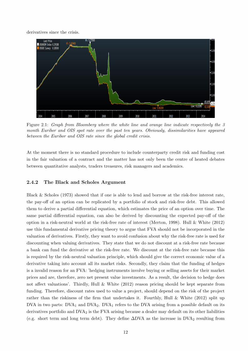
& White, 2013). Indeed, as illustrated in Figure 2.1, pre-crisis Euribor-OIS spread levels were very
small compared to post-crisis Euribor-OIS spread levels. So, as funding has become relatively more
costly and the interest received on collateral no longer offsets the funding cost, the FVA has become
non-negligible. This explains why FVA has been taking an increasingly important role in valuing
11
derivatives since the crisis.
Figure 2.1: Graph from Bloomberg where the white line and orange line indicate respectively the 3month Euribor and OIS spot rate over the past ten years. Obviously, dissimilarities have appearedbetween the Euribor and OIS rate since the global credit crisis.
At the moment there is no standard procedure to include counterparty credit risk and funding cost
in the fair valuation of a contract and the matter has not only been the centre of heated debates
between quantitative analysts, traders treasures, risk managers and academics.
2.4.2 The Black and Scholes Argument
Black & Scholes (1973) showed that if one is able to lend and borrow at the risk-free interest rate,
the pay-off of an option can be replicated by a portfolio of stock and risk-free debt. This allowed
them to derive a partial differential equation, which estimates the price of an option over time. The
same partial differential equation, can also be derived by discounting the expected pay-off of the
option in a risk-neutral world at the risk-free rate of interest (Merton, 1998). Hull & White (2012)
use this fundamental derivative pricing theory to argue that FVA should not be incorporated in the
valuation of derivatives. Firstly, they want to avoid confusion about why the risk-free rate is used for
discounting when valuing derivatives. They state that we do not discount at a risk-free rate because
a bank can fund the derivative at the risk-free rate. We discount at the risk-free rate because this
is required by the risk-neutral valuation principle, which should give the correct economic value of a
derivative taking into account all its market risks. Secondly, they claim that the funding of hedges
is a invalid reason for an FVA: ’hedging instruments involve buying or selling assets for their market
prices and are, therefore, zero net present value investments. As a result, the decision to hedge does
not affect valuations’. Thirdly, Hull & White (2012) reason pricing should be kept separate from
funding. Therefore, discount rates used to value a project, should depend on the risk of the project
rather than the riskiness of the firm that undertakes it. Fourthly, Hull & White (2012) split up
DVA in two parts: DVA1 and DVA2. DVA1 refers to the DVA arising from a possible default on its
derivatives portfolio and DVA2 is the FVA arising because a dealer may default on its other liabilities
(e.g. short term and long term debt). They define ∆DVA as the increase in DVA2 resulting from
12
the funding requirement of a derivatives portfolio with a particular counterparty. Assuming that the
CDS-bond basis is zero implies FVA = ∆DVA2. Lastly, Hull & White (2012) argue DVA2 does not
need to be calculated for most liabilities at inception because it is already reflected in the market
prices and hence FVA should be ignored.
2.4.3 Criticism on the Black and Scholes Argument
FVA has been the centre of intense debate between quantitative analysts, traders, treasurers and risk
managers. One controversial aspect of including FVA is that the law of one price is violated, which
is intolerable to some traditional quantitative analysts (Laughton & Vaisbrot, 2012). The banks
funding policy is an internal aspect, prices would become subjective, reflecting different funding
spreads of different banks Hull & White (2012). Nevertheless, many practitioners state this has been
a key factor driving bid-ask spreads and claim there is no way back to the pre-crisis world of unique
prices (Carver, 2012). As professor Damiano Brigo formulates it: ’In finance we’ve been trained to
think there is a Platonic price, one lesson of this crisis is that this law of one price is gone’ (Carver,
2012).
Furthermore, the Black and Scholes argument is less relevant since the global credit crisis Castagna
(2012). Pre crisis, many financial institutions were able to borrow (close to) the risk-free rate and
since the Black and Scholes argument hinges upon agents who are able to borrow at the risk-free
rate, the Black and Scholes PDE was valid. Nowadays, in practice banks typically borrow at a
higher rate than the risk-free rate. To illustrate this analytically, consider the classical Black and
Scholes argument, which is a consequence of replicating a derivative contract P by a portfolio of the
underlying S and bonds B. Following Castagna (2012):
Pt = αtSt + βtBt. (2.13)
Where, αt equals ∆t, the first derivative of the contract with respect to S and βt is chosen as
βt =Pt −∆tSt
Bt. (2.14)
S is assumed to to pay no dividend, so that
dPt = ∆tdSt + (Pt −∆tSt)rtdt, (2.15)
with rt = rt1{β>0} + rFt 1{β<0}. We denote with r the risk-free rate and with rF the funding rate
the bank has to pay on its debt. In the Black and Scholes argument it is assumed that, r = rF and
Eq. 2.15 equals the standard Black and Scholes PDE. However, in an economy where a bank pays a
higher interest rate than the risk-free rate when borrowing (β < 0), the Black and Scholes PDE in
Eq. 2.15 may contain the funding rate rF . Hence, always discounting by the same risk-free rate may
produce incorrect results, since it may not produce risk-neutral values corresponding to the costs of
the replication strategy. The Black and Scholes PDE can also be derived by discounting the expected
pay-off of a derivative in a risk-neutral world at the risk-free rate of interest (i.e. the fundamental
theorem of asset pricing). However, a necessary assumption to obtain the Black and Scholes PDE
13
is completeness, which means that every claim can be perfectly hedged. Nevertheless, in reality
markets are incomplete, portfolios cannot be perfectly hedged (Laughton & Vaisbrot, 2012).
Another important assumption in the reasoning of Hull & White (2012) is that the effect of a new
deal on the funding costs of a bank is linear (i.e. the linear funding feedback assumption). To
illustrate this assumption, consider a company that is worth 1 billion and has a credit spread or
funding spread of 100 basis points. Assume the company invests an additional 1 billion into a new
project which is risk-free. The linear funding feedback assumption implies that the company is now
worth 2 billion dollar and that its funding spread dropped to 50 basis point. Morini (2014) questions
this assumption, claiming the market funding feedback is highly non-linear. Consider for example
a firm in a distressed country that is very exposed to its sovereign. In the case that the credibility
of the sovereign stays the same, undertaking risk-free projects would merely decrease the funding
spread of the firms.
Lastly, many practitioners argue funding cost are real costs that can dramatically impact a banks
profit and loss statement. Hence, many big investment banks already implemented FVA. However,
there is still lots of controversy and all these bank calculate FVA in a different way (Cameron,
2014).
2.4.4 Double Counting and the Bond-CDS Basis
A very influential paper on the incorporation of FVA has been written by Morini & Prampolini
(2010). In this paper it is showed that the important variable determining the cost of liquidity is
neither the bond spread nor the credit default swap (CDS) spread, but the bond-CDS basis. In this
subsection the findings of Morini & Prampolini (2010) are briefly discussed.
Morini & Prampolini (2010) use a simple modeling setting, considering a deal involving a borrower
B and a lender L, where B commits to pay a fixed amount K to L at time T . Assume that party
X ∈ {B,L}, has a recovery rate RX . This means that in case of a default of party X, RX is the
percentage of the exposure that is recovered to creditors. The risk-free rate is denoted by r and is
assumed to be deterministic. Furthermore, X funds itself in the bond market and is the reference
entity in the CDS market. More generally, the CDS spread πX is assumed to be deterministic and
paid continuously. In Section 3.3.2 of Brigo et al. (2013) it is showed that in this case:
πX = λXLGDX . (2.16)
Where, λX denotes the deterministic default intensity and the loss given default LGDX equals 1−RX .
Recovery is assumed to be zero (LGDX = 1), thus πX = λX . From the exponential distribution
assumption for default time τ , it follows that P(τX > T ) = e−πXT (see section 3.3 of Brigo et al.
(2013)).
Like πX , the funding spread sX is also assumed to be instantaneous and deterministic. The cost
of funding is commonly measured in the secondary bond market as the spread over a risk-free rate.
The difference between the funding spread and the CDS spread of a party X is called the liquidity
basis and is denoted by γX , hence sX = πX + γX .
14
First, the net present value (NPV) for the lender VL of the above deal is described without includ-
ing funding cost. If P denotes the premium paid by L at inception, the NPV of the above deal
equals
VL = e−rTK − CV AL − P. (2.17)
Where CV AL is given by
CV AL = E[e−rTK1{τB≤T}]
= erTKP(τB ≤ T )
= e−rTK[1− e−πBT ]. (2.18)
To make the value of the contract fair we equate Eq. 2.17 to zero. Therefore, we have P = e−rTK −CV AL. From the perspective of the borrower, the NPV of the deal is
VB = −e−rTK +DV AB + P, (2.19)
with CV AL = DV AB. To make the value of the contract fair we set VB to zero, thus P = e−rTK −DV AB. Therefore, price symmetry is satisfied VB = VL = 0 and both parties may agree on the
premium of the deal:
P = e−rT e−πBK. (2.20)
Obviously, funding costs are not implemented in the above derivation. While L needs to finance the
claim P until the maturity of the deal at its funding spread sX , party B can reduce its funding by P .
Therefore, B has a funding benefit and party L needs to pay its financing cost and thus has funding
costs. Hence, party L should reduce the value of the claim by its financing costs. Besides, we cannot
assume both parties having negligible funding cost since we are dealing with possible default risk. To
introduce liquidity in the valuation of the deal, Morini & Prampolini (2010) describe the problem of
double counting. In this case, we implement liquidity costs by (only) changing the discount factor.
Moreover, the value to the lender is
VL = E[e−(r+sL)TK1{τB>T}]− P
= E[e−rT e−γLT e−πLTK1{τB>T}]− P
= e−rT e−γLT e−πLTKe−πBT − P, (2.21)
and the value to the borrower is
VB = −E[e−(r+sB)TK1{τB>T}] + P
= −E[e−rT e−γBT e−πBTK1{τB>T}] + P
= e−rT e−γBT e−2πBTK + P. (2.22)
To discuss this finding, we assume for simplicity that sL = 0, so the lender L is default-free and
has no liquidity basis. On the other hand, the borrower B may default, thus sB = πB > 0. In this
case we obtain PL = e−rT e−πBTK and PB = e−rT e−2πBTK, which is a remarkable finding. Firstly,
the two parties disagree on the premium of this simple deal. Borrowers can account an immediate
15
profit in all transaction with CVA. And secondly, pricing this deal at fair value to the borrower
would involve multiplying the NPV of K twice with its survival probabilities, which is called the
problem of double counting in Morini & Prampolini (2010). Both of these aspects belie years of
market reality.
In order to solve this puzzle, Morini & Prampolini (2010) model the funding strategy explicitly.
Following this approach, the deal is split up into two legs. From the lender’s perspective, the NPV
of the ‘deal leg’ is given by
E[−P + e−rTΠ], (2.23)
where Π denotes the pay-off at T with a potential default indicator. The other leg is called the
‘funding leg’ and NPV
E[P − e−rTF ], (2.24)
where F is the funding payment at T , also including a potential default indicator. Therefore, the
total NPV equals
VL = E[e−rTΠ− e−rTF ]. (2.25)
Morini & Prampolini (2010) make the assumption funding is made by issuing bonds and excess funds
are used to reduce or avoid increasing the stock of bonds. Therefore, the outflow F at T is
PerT esLT1{τL>T}. (2.26)
In the ’deal leg’, the lender inflow Π at T is K1{τB>T}. Thus, the total pay-off at T is
− PerT eγLT eπLT1{τL>T} +K1{τB>T}. (2.27)
Taking the discounted expectation of Eq. 2.27 yields
VL = −PeγLT +Ke−rT e−πBT . (2.28)
Analogously, it can be shown that the NPV of the deal for the borrower is
VB = PeγBT −Ke−rT e−πBT , (2.29)
where the double counting problem vanished. It can easily be shown that the break-even premium
for the lender is PL = Ke−rT e−πBT e−γLT and for the borrower PB = Ke−rT e−πBT e−γBT . To reach
an agreement: VL ≥ 0, VB ≥ 0, has to be satisfied, this implies PL ≥ P ≥ PB. Thus an agreement
can be found whenever, Ke−rT e−πBT e−γLT ≥ P ≥ Ke−rT e−πBT e−γBT , which holds when:
γB ≥ γL. (2.30)
This shows that, in order to have a positive NPV for both counterparties, the funding cost that
needs to be charged in this simplified transaction is just the liquidity basis. The lender’s funding
cost contains a part that is associated with the lender’s probability of default. This part cancels out
with the probability of default in the lender’s funding strategy, hence the only spread that contributes
as a net funding cost to the lender is the liquidity basis.
16
Chapter 3
Methodology
3.1 Interest Rate Model: G2++
To model the evolution of the Euribor rate (i.e. the underlying risk factor) we use a Gaussian shifted
two-factor process (hereafter G2++). This model is equivalent to the renowned Hull-White 2-factor
short rate model (Hull & White, 1994), only parametrized differently. To introduce this model we will
first show the single factor Hull-White process and discuss its limitations. Thereafter, we describe
the G2++ model and the associated calibration to market instruments. For basic theory regarding
interest rate modelling we refer to Chapters 3 and 4 of Brigo & Mercurio (2006).
3.1.1 Single Factor Hull-White Model
The single factor Hull-White model (Hull & White, 1990) is the forerunner of the G2++ model
and historically one of the most important interest rate models. The instantaneous short-rate r(t)
evolves according to the following stochastic differential equation:
dr(t) = (θ(t)− ar(t))dt+ σdW (t), (3.1)
where a indicates the rate of mean reversion to time-varying mean θ(t), σ is a volatility parameter
and W (t) a Brownian motion under the risk neutral measure Q. The model implies many convenient
features such as closed-form bond prices and a Gaussian distribution for the short-rate r. Though,
the model has an important disadvantage. To illustrate this disadvantage, consider the continuously
compounded spot interest rate R(t, T ) = − lnP (t,T )τ(t,T ) , which depends through P (t, T ) on the dynamics
of the short rate r(t). Moreover, consider a pay-off depending on the joint distribution of R(t, T1)
and R(t, T2), with T1, T2 > t and T1 6= T2. In the single factor Hull-White model the correlation
between R(t, T1) and R(t, T2) is 1, while in reality these rates are not perfectly correlated. The
model implies that shocks to the interest rate curve at time t are conveyed identically for different
maturities, which may be an unagreeable feature. Clearly, the pay-off of an IRS will depend on the
correlation between rates of different maturities. To overcome this problem of perfect correlation we
move to the G2++ model.
17
3.1.2 The G2++ Model
The G2++ model (Brigo & Mercurio, 2006) extends the single factor Hull-White model by assuming
the following stochastic differential equation for short-rate r(t):
dr(t) = x(t) + y(t) + ϕ(t), r(0) = r0, (3.2)
dx(t) = −ax(t)dt+ σdW1(t), x(0) = 0, (3.3)
dy(t) = −by(t)dt+ ηdW2(t), y(0) = 0. (3.4)
Where, r0, a, b, σ, η ≥ 0. Furthermore, W1,W2 are two correlated Brownian motions under Q with
dW1(t)dW2(t) = ρdt and ρ denoting the instantaneous correlation between these Brownian motions.
We use the G2++ model to model the instantaneous Euribor rates. The model enables analytical
formulae for various interest rate derivatives e.g. bond prices and swaptions, implies a Gaussian
distribution for short-rate r and allows for a non-perfect correlation structure between rates of
different maturities. A disadvantage of the G2++ model (and the single factor Hull-White model)
is the possibility of negative rates. Even so, the probability of negative interest rates is small
and as negative interest rates might occur in the current market environment we consider this
acceptable.
3.1.3 Calibration of the G2++ Model
To calibrate the G2++ model we first choose ϕ such that the model implied zero coupon bond prices
P (0, T ) equals the market observed term structure of discount factors PM (0, T ). In Section 4.2 of
Brigo & Mercurio (2006) it is showed that the G2++ model is fitted to the market observed term
structure of discount factor if and only if, for each T ,
ϕ(T ) = fM (0, T ) +σ2
2a2
(1− e−aT
)2+
η2
2b2
(1− e−bT
)2+ ρ
ση
ab
(1− e−aT
) (1− e−bT
), (3.5)
where fM (0, T ) = −∂ lnPM (0,T )∂T , i.e. the current market implied instantaneous forward rate for a
maturity T . Thence, we choose ϕ according to Eq. 3.5.
The model parameters a, b, σ, η and ρ are calibrated to market prices of at-the-money swaptions. A
swaption is (typically) an option on an interest rate swap, i.e. a swaption holder has the right, but
not the obligation to enter into an IRS at a pre-specified future date. A swaption is said to be at-the-
money when the fixed rate of the swaption (i.e. the strike of the swaption) equals the current swap
rate in the market. Given a strike rate X, strike date T , a nominal value N and payment schedule
T = {t1, ..., tn}, t1 > T , the G2++ model implies a arbitrage-free price for European swaptions. In
Brigo & Mercurio (2006) it is shown that this price, which we denote by ES, equals
ES(0, T, T , N,X, ω) = NP (0, T )ω
∫ ∞−∞
(1−
n∑i=1
ciA(T, ti)e−B(a,T,ti)x−B(b,T,ti)y
)+
f(x, y)dydx,
18
where ci = Xτi for i = 1, ..., n−1 and cn = 1+Xτn, ω = 1 (ω = −1) for a payer (receiver) swaption,
the density f of (x(T ), y(T )) is given by
f(x, y) =e− 1
2(1−ρ2xy)
[(x−µxσx
)2−2ρxy
(x−µx)(y−µy)σxσy
+(y−µyσy
)2]
2πσxσy√
1− ρ2xy
, (3.6)
and
µx = −MTx (0, T )
µy = −MTy (0, T )
σx = σ
√1− e−2aT
2a
σy = η
√1− e−2bT
2b
ρxy =ρση
(a+ b)σxσy
[1− e−(a+b)T
].
In order to calibrate the model, we choose the model parameters a, b, σ, η and ρ such that the sum
of the squared percentage differences between the model implied swaption volatilities and market
implied swaption volatilities are minimized. The implied swaption volatilities are calculated using
the Black formula for swaptions (Brigo & Mercurio, 2006).
3.2 Euribor-OIS Spread Model
Modelling the OIS rates with the G2++ model described in the previous section is troublesome, since
the calibration would be inaccessible. For example, there are no overnight index swaptions available
in the market. Instead of modelling the OIS rates themselves, OIS rates are obtained by modelling
the Euribor-OIS spread s. We have, s(t) = r(t) − c(t), where r(t) indicates the Euribor rate and
c(t) the OIS rate at time t. Theoretically, the Euribor-OIS spread should be a positive quantity as
the OIS rate should be lower than the associated Euribor rate. To model such an always-positive
process we adopt a CIR process, introduced by Cox et al. (1985), where we wish to simulate s(t) under
the risk-neutral measure Q. To do so, we first derive the Euribor-OIS spread dynamics under the
real-world measure P and subsequently account for the market price of risk to obtain the dynamics
under Q. We assume that the stochastic differential equation for the Euribor-OIS spread under the
real-world measure P is given by
ds(t) = κ(µ− s(t))dt+ ν√s(t)dW (t), (3.7)
where W is a standard Brownian motion under P and κ, µ, ν > 0. Moreover, κ corresponds to the
speed of mean reversion, µ to the mean and ν is a volatility parameter. We impose 2κµ > ν2 to keep
s(t) positive. Likewise, we assume that the dynamics under Q are given by
ds(t) = κ(µ− s(t))dt+ ν√s(t)dW (t), (3.8)
19
where W is a standard Brownian motion under Q and κ, µ, ν > 0. We adopt a similar methodology
as in Cox et al. (1985), and set κ = κ+ λ, µ = (κµ)κ+λ and ν = ν, where λ denotes the market price of
risk.
3.2.1 Calibration of the Euribor-OIS Spread Model
In order to calibrate the Euribor-OIS spread model, we first calibrate the model parameters κ, µ, ν
to historical market data of Eonia and Euribor spot rates. Consider the Euler discretization of Eq.
3.7:
s(t+ δt) = s(t) + κ(µ− s(t))δt+ ν√s(t)Z(t), (3.9)
where Z is a standard-normal random variable. Equivalently,
s(t+ δt)− s(t)√s(t)
=κµδt√s(t)− κ√s(t)δt+ νZ(t). (3.10)
Note that the above equation can be seen as a linear regression model with dependent variables(t+δt)−s(t)√
s(t)and explanatory variables δt√
s(t)and δt
√s(t). Therefore, κµ, κ and ν can be estimated
consistently by Ordinary Least Squares.
Thereafter, we estimate the market price of risk λ by minimizing the sum of squared differences
between a set of model implied bond prices and market implied bond prices. As in Hull (2009), the
bond price PCIR(t, T ) implied by the CIR model, is given by
PCIR(t, T ) = A(t, T )e−B(t,T )s(t), (3.11)
where,
A(t, T ) =2he
12
(κ+h)(T−t)
2h+ (κ+ h)(eh(T−t) − 1)
2kµ
ν2
, (3.12)
B(t, T ) =2(eh(T−t) − 1)
2h+ (κ+ h)(eh(T−t) − 1)(3.13)
and h =√κ2 + 2ν2. Since we are modelling the spread between the two instantaneous interest rates
r(t) and c(t), the relevant market implied bond prices are given by
PMKT (t, T ) = EQ[e−∫ Tt (r(u)−c(u))du]. (3.14)
Note that theoretically, a bond prices is just the risk neutral expectations of the relevant discount
factors. Moreover, we can write Eq. 3.14 as the risk neutral expectation of a quotient of two stochastic
discount factors
PMKT (t, T ) = EQ
[e−∫ Tt r(u)du
e−∫ Tt c(u)du
]= EQ
[Deur(t, T )
Dois(t, T )
], (3.15)
where Deur and Dois are the stochastic discount factors of the instantaneous Euribor and OIS rate
20
respectively. Equivalently, we can write Eq. 3.15 as
PMKT (t, T ) =EQ [Deur(t, T )]
EQ [Dois(t, T )]+ cov
[Deur(t, T ),
1
Dois(t, T )
]. (3.16)
Using historical data, we can estimate the latter covariance term, which we find to be negligible
in magnitude. Nevertheless, we do include the term in the calculation. Note that we can view
the former term of Eq. 3.16 as a quotient of two bond prices as Peur(t, T ) = EQ [Deur(t, T )] and
Pois(t, T ) = EQ [Dois(t, T )], which are market observable.
To estimate the market price of risk, we vary λ to minimize the sum of squared differences be-
tween the current model implied bond prices PCIR(0, T ) and the current market implied bond prices
PMKT (0, T ), for a set of different maturities. When we have estimated λ we can determine κ and µ
by κ = κ+ λ and µ = (κµ)κ+λ .
3.3 Credit Spread Model
3.3.1 Stochastic Intensity
Possible default events are modelled by a stochastic intensity model called the CIR++ model.
Stochastic intensity models describe default time τ as the first jump time of a Cox process, that
is a Poisson process with stochastic intensity. The basic idea behind these models is that default
has an exogenous element, which is independent of market observables. Indeed, market data does
not give complete information on the default process. Therefore, intensity λt is assumed to be
time-varying and stochastic. More explicit, having not defaulted before time t, the probability of
defaulting in the next time instant dt is λtdt. Thereby, we will often use the cumulated intensity
Λ =∫ t
0 λ(u)du. This sort of default models are well-suited to model credit spreads and calibration
to Credit Default Swap (CDS) data is well-to-do (Brigo & Mercurio, 2006).
To show why these models are well suited for credit spreads, suppose for simplicity deterministic
intensity λ. An peculiarity of Poisson processes is a result of the transformation of jump time τ
according to its own cumulated intensity Λ (Brigo & Mercurio, 2006). Hence, Λ(t) = ξ ∼ exponential
standard random variable. Inverting this result yields τ = Λ−1(ξ). By recalling Q(ξ ≤ x) = 1− e−x,
i.e. the cumulative distribution function of an exponential standard random variable, we have
Simulating the (correlated) stochastic processes used to calculate BCVA and FVA involves sampling
random shocks from a multivariate normal distribution. A requirement for the covariance matrix
of this multivariate normal distribution is positive-semidefiniteness. Unfortunately, performing the
methodologies described, we may obtain a covariance matrix which fails to be positive-semidefinite.
For example, in cases of strong wrong-way risk the covariance matrix may fail to meet the requirement
of positive-semidefiniteness. To overcome this undesirable aspect, we use Hypersphere decomposition
described by Rebonato & Jackel (1999). This method transforms the original matrix to a similar
positive-semidefinite one, insuring unit diagonals and symmetry, which is required for simulating
Brownian motions. Rebonato & Jackel (1999) also show that Hypersphere decomposition almost
26
always leads to very small differences between the original and transformed matrix.
3.4.4 The Equation for Bilateral Credit Value Adjustment
Consider a transaction involving two default risky entities: a bank bnk and a corporate cpt. The NPV
of the transaction at time t with maturity date T (without taking into account corporate default
risk) is V (t, T ) and we wish to find V (t, T ), the adjusted value of the derivative, subject to corporate
default risk. Besides, the BCV A(t, T ) is the difference between V (t, T ) and V (t, T ). We will address
valuations from the perspective of the bank, hence cash flows received by bnk (and paid by cpt) will
be positive whereas cash flows paid by bnk (and received by cpt) will be negative. Furthermore,
τbnk and τcpt indicate the default times of respectively bnk and cpt. In the same way, RECbnk and
RECcpt denote their recovery fractions (i.e. the percentage of the claim that is recovered in case the
associated entity defaults). Lastly, denote the first-to-default time as τ1 = min(τbnk, τcpt). To find
V (t, T ), we may distinguish three cases:
1. Neither bank nor corporate defaults before T ,
2. The corporate defaults first and before T ,
3. The bank defaults first and before T .
In the first case, the corresponding (risky) payoff is
1{τ1>T}V (t, T ), (3.31)
where 1{τ1>T} equals 1 if τ1 > T and 0 otherwise. In the second case, the cash flows paid up to the
default time are paid plus the pay-off at default. Hence, the payoff equals
1{τcpt≤T}V (t, τcpt) + 1{τ1≤T}1{τcpt=τ1}(RECcptV (τ1, T )+ + V (τ1, T )−), (3.32)
where V − = min(V, 0) and V + = max(V, 0). Note that in this case bnk pays the risk-free value of the
derivative to cpt if it is negative, i.e. when bnk is a debtor and cpt is a creditor. On the other hand,
when the risk-free value of the derivative is positive at τcpt, bnk only receives a recovery fraction
of the risk-free value of the derivative from the defaulted corporate cpt. Likewise, the payoff in the
third case equals
1{τbnk≤T}V (t, τbnk) + 1{τ1≤T}1{τbnk=τ1}(RECbnkV (τ1, T )− + V (τ1, T )+). (3.33)
By summing the above payoffs the adjusted value of the derivative, subject to corporate default risk
is
V (t, T ) = EQ[1{τ1>T}V (t, T )
+ 1{τ1≤T}V (t, τ1)
+ 1{τ1≤T}1{τcpt=τ1}(RECcptV (τ1, T )+ + V (τ1, T )−)
+ 1{τ1≤T}1{τbnk=τ1}(RECbnkV (τ1, T )− + V (τ1, T )+)],
27
where EQ denotes the expectation under the risk-neutral probability measure. The above expression
can be written as
V (t, T ) = EQ[1{τ1≤T}V (t, T )
+ 1{τ1≤T}V (t, τ1) + 1{τcpt=τ1}V (τ1, T ) + 1{τbnk=τ1}V (τ1, T )
+ 1{τ1≤T}1{τcpt=τ1}(RECcptV (τ1, T )+ − V (τ1, T )+)
+ 1{τ1≤T}1{τbnk=τ1}(RECbnkV (τ1, T )− + V (τ1, T )−)].
Thence, we can write
V (t, T ) = V (t, T )− EQ[1{τ1≤T}1{τcpt=τ1}(1−RECcpt)V (τ1, T )+
+ 1{τ1≤T}1{τbnk=τ1}(1−RECbnk)V (τ1, T )−].
Recall from Subsection 2.3.2, that V = V + BCV A and notice that the latter term in the above
equation expresses BCVA. Thus, the equation for BCVA is
BCV A(t, T ) = −EQ[1{τ1≤T}1{τcpt=τ1}(1−RECcpt)V (τ1, T )+ (3.34)
+ 1{τ1≤T}1{τbnk=τ1}(1−RECbnk)V (τ1, T )−].
Throughout this thesis, we assume deterministic recovery fractions and no simultaneous defaults.
Hence,
BCV A(t, T ) = −(1−RECcpt)EQ[1{τ1≤T}1{τcpt=τ1}V (τ1, T )+] (3.35)
− (1−RECbnk)EQ[1{τ1≤T}1{τbnk=τ1}V (τ1, T )−].
To simplify the above expression furthermore, we need to make assumptions regarding the depen-
dence structure of default events and exposure. When credit quality and exposure are assumed to be
independent, the terms in Eq. 3.35 can be split up in different expectations, which can be multiplied
to calculate BCVA. In this case, we obtain,
BCV A(t, T ) = −(1−RECcpt)EQ[1{τ1≤T}1{τcpt=τ1}]EQ[V (τ1, T )+] (3.36)
− (1−RECbnk)EQ[1{τ1≤T}1{τbnk=τ1}]EQ[V (τ1, T )−].
In general, we will refer to Expected Exposure as EE(t, T ) = EQ[V (t, T )+], whilst Negative Expected
Exposure is given by NEE(t, T ) = EQ[V (t, T )−]. Besides, the risk-neutral survival probability
of entity i in the interval [t, T ] is given by S(t, T )i = EQ[τi > T ]. Note that the risk-neutral
default probability in this interval is 1 − S(t, T ). Furthermore, recall from Subsection 2.3.2, that
BCV A = DV A − CV A. Indeed, as in Gregory (2013), in case of no wrong-way risk (which is
28
discussed in the next subsection), CVA is given by
CV A(t, T ) = (1−RECcpt)EQ[1{τ1≤T}1{τcpt=τ1}]EQ[V (τ1, T )+], (3.37)
and DVA is given by
DV A(t, T ) = −(1−RECbnk)EQ[1{τ1≤T}1{τbnk=τ1}]EQ[V (τ1, T )−].
3.4.5 Wrong- and Right-way Risk
Wrong-way risk and right-way risk are phrases that are generally used to indicate dependence between
exposure and counterparty credit quality (Gregory, 2013). In case this dependence is unpropitious,
we speak of wrong-way risk. Whereas, in the case of a propitious dependence structure between
exposure and counterparty credit quality, we spreak of right-way risk. For interest rate swaps, one
should consider a relation between interest rates and counterparty credit quality. High interest rates
might cause (leveraged) firms to default, while low interest rates could indicate a recession where
default events are more common. We analyse this effect by correlating the short rate factors of the
G2++ model with the intensity process embedded in the CIR++ model. Moreover, we allow for
an instantaneous correlation between the associated driving Brownian motions W1, W2 and Z as in
Brigo & Mercurio (2006), hence d〈Wi, Z〉t = ρidt, i ∈ {1, 2}. In this case, the resulting correlation
between interest rates and credit spreads becomes
ρi =d〈r, λ〉t√
d〈r, r〉td〈λ, λ〉t=
σρ1 + ηρ2√σ2 + η2 + 2σηρ12
, (3.38)
where ρ12 denotes the instantaneous correlation between W1 and W2. To limit the number of free
parameters we always set ρ1 = ρ2. Finally, by varying ρi we may allow for wrong- and right-way
risk.
3.5 Modelling Funding Value Adjustment
The occurrence of and the reasons why there is so much dissension surrounding FVA are discussed in
Section 2.4. As a matter of fact, all banks that have incorporated FVA calculate it in different ways
(Cameron, 2014). Meanwhile, some banks choose to ignore FVA, while other banks just do not know
how to handle FVA. It may be clear that there is a great need for a market practice regarding the
implementation of FVA. In this section we propose and motivate a method to implement FVA for an
uncollaterlized plain vanilla interest rate swap. We assume stochastic net funding cost, modelled by
a CIR process. To avoid the problem of double counting we define net funding cost as the Bond-CDS
basis plus a fixed premium representing the internal treasury’s lending rate. In order to describe
these aspects, we use the same setting and notation as in Subsection 3.4.4.
29
3.5.1 The Equation for Funding Value Adjustment
The purpose of the incorporation of FVA is to include the funding cost related to the ’production’ of
a derivative’s transaction, i.e. the cost of funding the corresponding hedge over the maturity of the
deal. Consider the bank bnk and the corporate cpt enter in an uncollaterlized plain vanilla interest
rate swap. The bank perfectly hedges the uncollaterlized transaction by entering in a secured trans-
action with an underlying CSA in the interbank market. We name the counterparty in this ’hedge
deal’ Bank B. Note that this is a typical situation, as the corporate generally requests the bank for
an uncollaterlized transaction and not vice versa. As a matter of fact, the operational implications
of CSA’s are often unmanageable for corporates (Cameron, 2014). Therefore, we do not consider a
bilateral FVA, as proposed by Gunnesson & Moreles (2014). To limit complexity, we suppose the
CSA specifies that cash is the only valid collateral and that the Euro is the only valid currency
in which this cash can be posted. Besides, we assume that the collateral rate is the Eonia rate.
Moreover, we suppose that in order to trade collateral the bank’s trading desk needs to borrow funds
from the bank’s treasury desk. The associated internal treasury’s lending rate is the cost of funding
for the bank’s trading desk and includes (for example) internal labor, system and administration
costs. Lastly, we assume that the bank’s treasury desk funds itself by issuing bonds in the (money)
market.
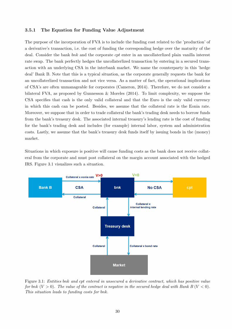
Situations in which exposure is positive will cause funding costs as the bank does not receive collat-
eral from the corporate and must post collateral on the margin account associated with the hedged
IRS. Figure 3.1 visualizes such a situation.
Figure 3.1: Entities bnk and cpt entered in unsecured a derivative contract, which has positive valuefor bnk (V > 0). The value of the contract is negative in the secured hedge deal with Bank B (V < 0).This situation leads to funding costs for bnk.
30
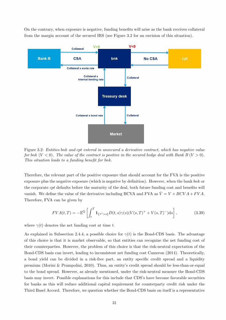
On the contrary, when exposure is negative, funding benefits will arise as the bank receives collateral
from the margin account of the secured IRS (see Figure 3.2 for an envision of this situation).
Figure 3.2: Entities bnk and cpt entered in unsecured a derivative contract, which has negative valuefor bnk (V < 0). The value of the contract is positive in the secured hedge deal with Bank B (V > 0).This situation leads to a funding benefit for bnk.
Therefore, the relevant part of the positive exposure that should account for the FVA is the positive
exposure plus the negative exposure (which is negative by definition). However, when the bank bnk or
the corporate cpt defaults before the maturity of the deal, both future funding cost and benefits will
vanish. We define the value of the derivative including BCVA and FVA as V = V +BCV A+FV A.
Therefore, FVA can be given by
FV A(t, T ) = −EQ[∫ T
t1{τ1>s}D(t, s)γ(s)(V (s, T )+ + V (s, T )−)ds
], (3.39)
where γ(t) denotes the net funding cost at time t.
As explained in Subsection 2.4.4, a possible choice for γ(t) is the Bond-CDS basis. The advantage
of this choice is that it is market observable, so that entities can recognize the net funding cost of
their counterparties. However, the problem of this choice is that the risk-neutral expectation of the
Bond-CDS basis can invert, leading to inconsistent net funding cost Cameron (2014). Theoretically,
a bond yield can be divided in a risk-free part, an entity specific credit spread and a liquidity
premium (Morini & Prampolini, 2010). Thus, an entity’s credit spread should be less-than-or-equal
to the bond spread. However, as already mentioned, under the risk-neutral measure the Bond-CDS
basis may invert. Possible explanations for this include that CDS’s have become favorable securities
for banks as this will reduce additional capital requirement for counterparty credit risk under the
Third Basel Accord. Therefore, we question whether the Bond-CDS basis on itself is a representative
31
quantity of a bank’s funding cost. In fact, internal lending rates also affect funding cost. From a
bank’s internal perspective the treasury desk typically lends money to the trading desks. Hence, the
bank’s treasury desk acquires funds in the market, while the trading desks obtains funds from the
treasury desk. The internal treasury’s lending rate is the cost of funding for the derivatives desk. For
example labour, system and administration costs may be included in the internal treasury’s lending
rate. Obviously, this rate affects FVA, but as it is not market observable other entities might not
recognize a FVA based on this rate.
In order to model FVA we take the internal treasury’s lending rate F fixed and specify the net
funding cost at time t as
γ(t) = b(t)− c(t)− π(t) + F, (3.40)
where b denotes the banks bond yield, c the collateral rate and π the banks credit spread. Note that
the credit spread π enters the equation to avoid double counting.
3.5.2 Net Funding Cost Model: CIR Process
In Section 3.2 we described how a CIR process can be used to model the Euribor-OIS spread. To
model the net funding cost γ(t) we use a similar approach. This approach is suitable in the sense
that net funding cost are assured to stay positive. Moreover, net funding costs are assumed to be
time-varying and the model can be calibrated in a convenient way to market data. We assume the
net funding cost γ(t) evolve according to the CIR process
dγ(t) = κ(µ− γ(t))dt+ ν√γ(t)dW (t), (3.41)
where W is a standard Brownian motion under P and κ, µ, ν > 0. Moreover, κ corresponds to the
speed of mean reversion, µ to the mean and ν is a volatility parameter. We impose 2κµ > ν2 to keep
γ(t) positive. Likewise, we assume that the dynamics under Q are given by
dγ(t) = κ(µ− γ(t))dt+ ν√γ(t)dW (t), (3.42)
where W a standard Brownian motion under Q and κ, µ, ν > 0. We adopt a similar methodology as
in Section 3.2, and set κ = κ+λ, µ = (κµ)κ+λand ν = ν, where λ denotes the market price of risk.
3.5.3 Calibration of the Net Funding Cost Model
In order to calibrate the net funding cost model, we first calibrate the model parameters κ, µ, ν
to historical market data of bond yields, Eonia spot rates and credit spreads. Consider the Euler
where Z a standard-normal random variable. Equivalently,
γ(t+ δt)− γ(t)√γ(t)
=κµδt√γ(t)
− κ√γ(t)δt+ νZ(t). (3.44)
Note that the above equation can be seen as a linear regression model with dependent variableγ(t+δt)−γ(t)√
γ(t)and explanatory variables δt√
γ(t)and δt
√γ(t). Therefore, κµ, κ and ν can be estimated
consistently by Ordinary Least Squares.
Thereafter, we estimate the market price of risk λ by minimizing the sum of squared differences
between a set of model implied bond prices and market implied bond prices. The model implied
bond price PCIR(t, T ) model, is given by Eq. 3.11 with s(t) replaced by γ(t). The relevant market
implied bond price is given by
PMKT (t, T ) = EQ[e−∫ Tt γ(u)du
]= EQ
[e−∫ Tt (b(u)−c(u)−π(u)+F )du
]. (3.45)
Note that theoretically, a bond price is just the risk-neutral expectation of the relevant discount
factors. We assumed that the internal treasury’s lending rate F is fixed, thus independent of the
credit spread π. Nevertheless, we want to note that there might be a relation between internal
lending rates and credit spreads, as the treasury desk of a distressed bank might ask higher interest
from the relevant derivative desks. However, this aspect is beyond the scope of this thesis, hence we
leave it for future research. Furthermore, we can rewrite Eq. 3.45 as
PMKT (t, T ) = e−F (T−t)EQ
[e−∫ Tt b(u)−c(u)du
e−∫ Tt π(u)du
]
= e−F (T−t)EQ[e−∫ Tt b(u)−c(u)du
]EQ[e−∫ Tt π(u)du
] + cov
[e−∫ Tt b(u)−c(u)du,
1
e−∫ Tt π(u)du
]. (3.46)
Using historical data, we can estimate the latter covariance term. The two risk-neutral expectations
in the former term can be calculated using current bond yields, Eonia spot rates and credit spread
data. In more detail, by definition the zero coupon bond curve at time t is EQ[∫ Tt b(u)du
], the Eonia
yield curve at time t equals EQ[∫ Tt c(u)du
]and the market CDS curve at time t is EQ
[∫ Tt π(u)du
],
where T corresponds to the associated (market observable) maturities.
To estimate the market price of risk, we vary λ to minimize the sum of squares differences between
the current model implied bond prices PCIR(0, T ) and the current market implied bond prices
PMKT (0, T ), for a set of different maturities. After estimating λ we can determine κ and µ by
κ = κ+ λ and µ = (κµ)κ+λ . Hence, Monte Carlo integration can be used to calculate the expected net
funding cost under the risk-neutral measure, which is needed to calculate FVA.
33
Chapter 4
A Case Study
To analyze FVA in the fair valuation of interest rate swaps, we examine a common situation, where
a bank and a corporate enter into a plain vanilla interest rate swap. Moreover, we want to adjust
the price of this swap for counterparty credit risk and funding risk by calculating BCVA and FVA.
We question what the total value adjustment (TVA) should be, where TV A = BCV A + FV A.
Hence, by applying the described methodology we calculate BCVA and FVA. Thereby, we perform
an impact analysis as the calculations of BCVA and FVA are highly model dependent. Hence, we
analyse the impact of wrong-way risk, credit spread levels and credit spread volatilities on BCVA
and FVA.
4.1 Case Description
Suppose Koninklijke Ahold NV (AH) wants to hedge its interest rate risk by entering into a plain
vanilla interest rate swap with Deutsche Bank AG (DB). AH proposes the following conditions
regarding the swap:
• AH pays a fixed interest rate of 1.76% and receives 3 month Euribor (this makes the initial
value of the swap zero)
• DB pays 3 month Euribor and receives a fixed rate of 1.76%
• Both fixed rate and floating rate payments occur quarterly
• The principal amount is 10,000,000 euro
• The maturity of the swap is 10 years
• All payments are made in euros
April 30, 2014 is both the valuation date and the start date of the swap, hence the first payments
associated with the swap will be made on 30 July 2014. Note that no CSA underlying the swap
is proposed, which means the swap would be uncollateralized. The bank and the corporate enter
into negotiations to discuss the fair price of the swap. Both parties agree that the price of the swap
involves discounting the floating leg payments and the fixed leg payments using the Eonia curve.
34
Besides, both parties recognize that since there is no CSA involved in the deal, both parties will
have significant credit risk towards each other, hence a CVA and DVA will be incorporated in the
fair price of the swap. Thereby, DB argues that funding cost may arise when it hedges the trade
in the interbank market via a collateralized swap, as these cost are part of the construction of the
deal, they should be incorporated in the price. Hence, the bank proposes the incorporation of a FVA
for the expected funding costs the bank will have over the maturity of the swap. The bank would
calculate the FVA along with BCVA, by modelling the CDS-bond basis, which should avoid double
counting. Thereby, the bank will add a mark up to FVA for the internal transfer cost of the bank
(F = 0.005). The case questions are, what should be the total value adjustment (TVA)? Where,
TV A = BCV A+FV A, and how sensitive are BCVA, FVA and TVA to changes in wrong-way risk,
credit spread levels and credit spread volatilities?
4.2 Data
We obtained all needed market data from Bloomberg, observed on April 30, 2014. To start with, we
obtained the Eonia curve, which represents the market discount curve and the 3 month Euribor curve,
which is used to calculate the floating leg of our swap. Thereby, we use historical Eonia spot rates
and 3 month Euribor spot rates to model the Euribor-OIS spread. The historical rates are observed
between April 30, 2010 and April 30, 2014. Furthermore, we obtained market euro at-the-money
swaption volatilities to calibrate the G2++ model. Besides, to bootstrap market implied survival
and default probabilities, we obtained the euro senior CDS curve for both Koninklijke Ahold NV
and Deutsche Bank AG. Lastly, we also obtained current and historical (zero-coupon) bond yields
of Deutsche Bank to calculate FVA. More detailed information regarding the market data can be
found in Appendix A.
4.3 Research Approach
Firstly, we calibrate the model parameters of the G2++ model, the Euribor-OIS spread model,
the CIR++ model and net funding cost model to our market data, according to the methodology
described in respectively Subsections 3.1.3, 3.2.1, 3.3.2 and 3.5.3. Subsequently, we simultaneously
simulate the relevant stochastic processes 1000 times. For each generated scenario, we calculate
exposures, default probabilities and survival probabilities. By doing this, we can calculate the BCVA
according to Eq. 3.35], where the expectations are approximated using Monte Carlo integration.
Likewise, the FVA is calculated according to Eq. 3.39.
35
Chapter 5
Results
In this chapter we document the results of the case study by applying the described methodology. We
provide calibration results including parameter estimations, relevant graphs and ratios to indicate
the goodness of fit. Thereby, we provide the results of the impact analysis in the form of tables and
graphs.
Without taking wrong- and right-way risk into account, we estimate a FVA of 40,661 euro and a
BCVA of 26,126 euro adding up to a TVA of 66,787. Hence, by incorporating FVA and BCVA the
fair value of the swap becomes 0+66, 787 = 66, 787 euro. Thus, by incorporating counterparty credit
risk and funding risk, Deutsche Bank can see the swap as an asset rather than a liability. On the
contrary, Ahold can regard the swap as a liability. To explain this finding, we report the exposure
profiles plotted in Figure 5.1.
Figure 5.1: Expected Exposure (EE(0, T )) and Negative Expected Exposure (NEE(0, T )) for DeutscheBank corresponding with the receiver IRS described in the case study. Expected Positive Exposure(EPE) and Expected Negative Exposure (ENE) are the averages of respectively EE and NEE.
36
Clearly the NEE is on average higher in absolute value than the EE. This indicates that on average
Ahold has more exposure to Deutsche Bank than vice versa. Thus, given that the two entities have
similar survival probabilities (see Figure 5.6), the DVA term will be greater than the CVA term
and so BCVA will be positive (26,126 euro). Likewise, the fact that ENE is higher than EPE in
absolute value implies that it is more likely for Deutsche Bank to have a funding benefit than funding
costs. Hence, there is an expected funding benefit, indicating a similar scenario as in Figure 3.2 will
occur. This reasoning follows from the formula for FVA in Eq. 3.39. Therefore, we observe a positive
FVA (40,661 euro). Recall that we defined: Fair Value = NPV + BCVA + FVA, so that both the
positive BCVA term and the positive FVA will contribute to a higher Fair Value, i.e. the value of
the swap taking into account both funding and credit risk.
5.1 Calibration
In this section the calibration results of our stochastic models are documented. We provide inter alia
parameter estimations, relevant graphs and ratios to indicate the goodness of fit.
5.1.1 G2++ Model Parameters
In order to perform the calibration of the G2++ model parameters we use the methodology described
in Subsection 3.1.3. We use the current market observed Euribor curve and euro at-the-money swap-
tion volatilities to calibrate the G2++ model. Moreover, by varying the model parameters (a, b, σ, η
and ρ), we minimize the sum of squares of the percentage differences between the model and market
implied swaption volatilities. The calibration produces the following parameter estimates:
a = 0.351447 b = 0.001812 σ = 0.010573 η = 0.008802 ρ = −0.988529. (5.1)
To give an indication of the goodness of fit, we report in Figure 5.2 the calibration errors in the form
of percentage differences between the model and market implied swaption volatilities.
37
Figure 5.2: Calibration errors associated with the G2++ model, the calibration errors are percentagedifferences between model and market implied swaption volatilities.
The standard deviation of the calibration errors is 2,82%. Moreover, the absolute average mispricing
regarding the calibration is 2,28%, which we consider fairly small.
5.1.2 Euribor-OIS Spread Model Parameters
We calibrate the Euribor-OIS spread model parameters according to the methodology described in
Subsection 3.2.1. We use historical daily market data of Euribor and OIS bond prices over the past
4 years (1027 observations) to obtain the model parameters under P. Afterwards, we use current
Euribor and OIS bond prices to determine the market price of risk λ. By doing this, we may adjust
the real-world parameter estimates to risk-neutral parameter estimates. The resulting risk-neutral
parameter estimates are
κ = 2.0771 µ = 0.0022 ν = 0.0464, (5.2)
and for the market price of risk we obtain λ = 1.3292. To give an indication of the magnitude of
the estimation error of λ we also report the root mean squared error (RMSE), which equals 0.0081.
Although, the RMSE is not negligibly small, we consider this estimation error to be acceptable.
Moreover, we provide the model and market implied bond prices stemming from the calibration
procedure in Figure 5.3.
38
Figure 5.3: The market implied bond price PMKT and the (fitted) model implied bond price PCIR
(evaluated at λ = 1.3292).
5.1.3 CIR++ Model Parameters
To calibrate the CIR++ model, we first bootstrap market implied default intensities and survival
probabilities from CDS data of Deutsche Bank AG and Koninklijke Ahold NV as described in
Subsection 3.3.2. In Figures 5.4 and 5.5 we show the resulting market implied default intensities of
respectively Deutsche Bank and Ahold.
Figure 5.4: Market implied piecewise constant default intensity γ of Deutsche Bank, stripped fromCDS data on April 30, 2014.
39
Figure 5.5: Market implied piecewise constant default intensity γ of Ahold, stripped from CDS dataon April 30, 2014.
From these graphs we may construct risk-neutral survival probabilities which we report in Figure
5.6. Note that the market regards Ahold slightly default riskier than Deutsche Bank over the long
term (10 years). Next we use Eq. 3.24 to fit the term structure of credit spreads of both Deutsche
Bank and Ahold to the CIR++ model.
Finally, we are left with the CIR parameter vector β which can be calibrated to other securities.
However, this is tricky since the current market for CDS options is lacking liquidity. Therefore, we
choose reasonable values for β, in accordance with the estimates of Brigo & Mercurio (2006), which
uses a hypothetical implied volatility surface of CDS options. We set
κ = 0.354201 µ = 0.001219 ν = 0.023819, (5.3)
for both Ahold and Deutsche Bank. In Section 5.2 we vary µ and ν to analyse the impact of,
respectively, credit spread levels and credit spread volatilities on BCVA and FVA. Calibrating the
CIR++ model parameters to real market data is left for future research.
Figure 5.6: Risk-neutral survival probabilities of Deutsche Bank (DB) and Ahold (AH)
40
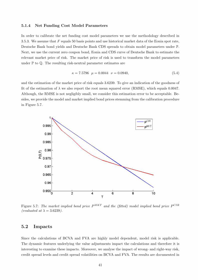
5.1.4 Net Funding Cost Model Parameters
In order to calibrate the net funding cost model parameters we use the methodology described in
3.5.3. We assume that F equals 50 basis points and use historical market data of the Eonia spot rate,
Deutsche Bank bond yields and Deutsche Bank CDS spreads to obtain model parameters under P.
Next, we use the current zero coupon bond, Eonia and CDS curve of Deutsche Bank to estimate the
relevant market price of risk. The market price of risk is used to transform the model parameters
under P to Q. The resulting risk-neutral parameter estimates are
κ = 7.5796 µ = 0.0044 ν = 0.0940, (5.4)
and the estimation of the market price of risk equals 3.6239. To give an indication of the goodness of
fit of the estimation of λ we also report the root mean squared error (RMSE), which equals 0.0047.
Although, the RMSE is not negligibly small, we consider this estimation error to be acceptable. Be-
sides, we provide the model and market implied bond prices stemming from the calibration procedure
in Figure 5.7.
Figure 5.7: The market implied bond price PMKT and the (fitted) model implied bond price PCIR
(evaluated at λ = 3.6239).
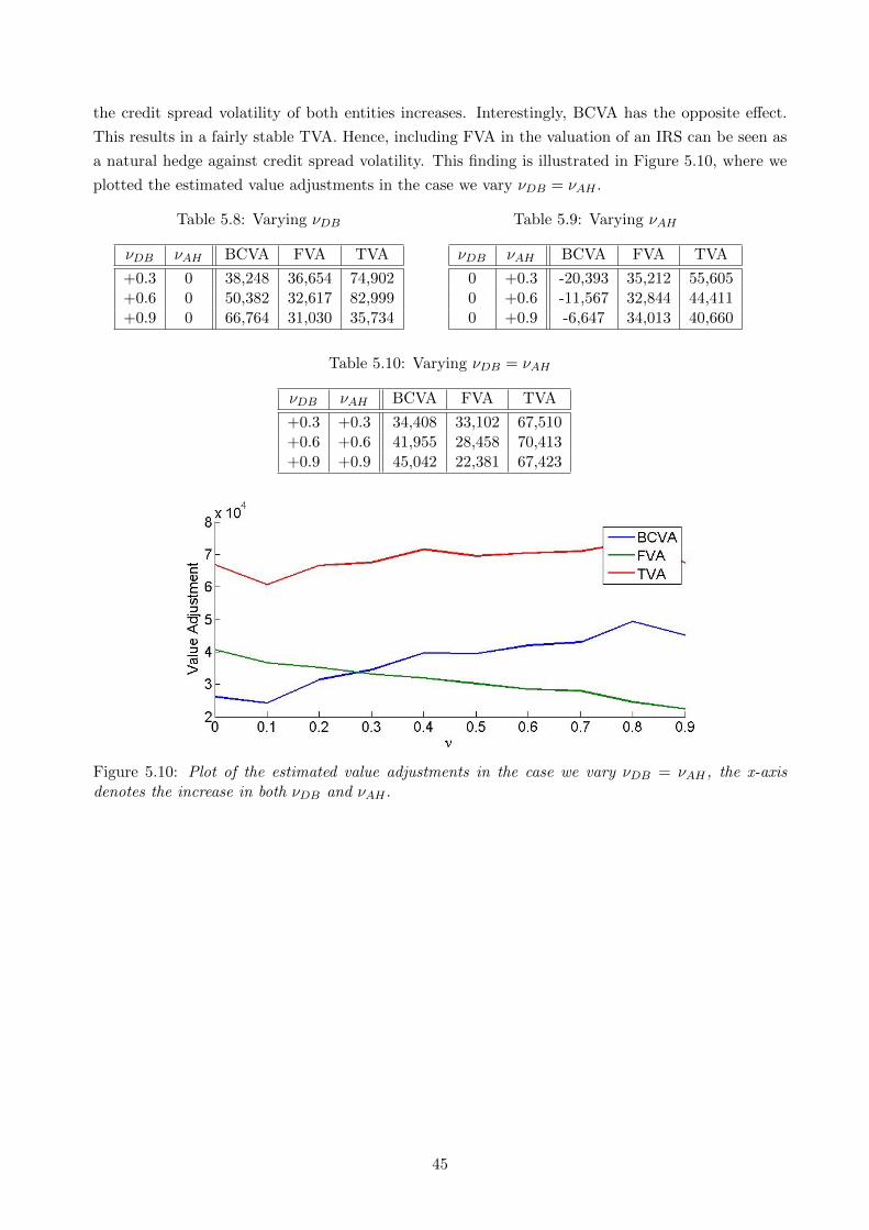
5.2 Impacts
Since the calculations of BCVA and FVA are highly model dependent, model risk is applicable.
The dynamic features underlying the value adjustments impact the calculations and therefore it is
interesting to examine these impacts. Moreover, we analyse the impact of wrong- and right-way risk,
credit spread levels and credit spread volatilities on BCVA and FVA. The results are documented in
41
the form of tables and graphs.
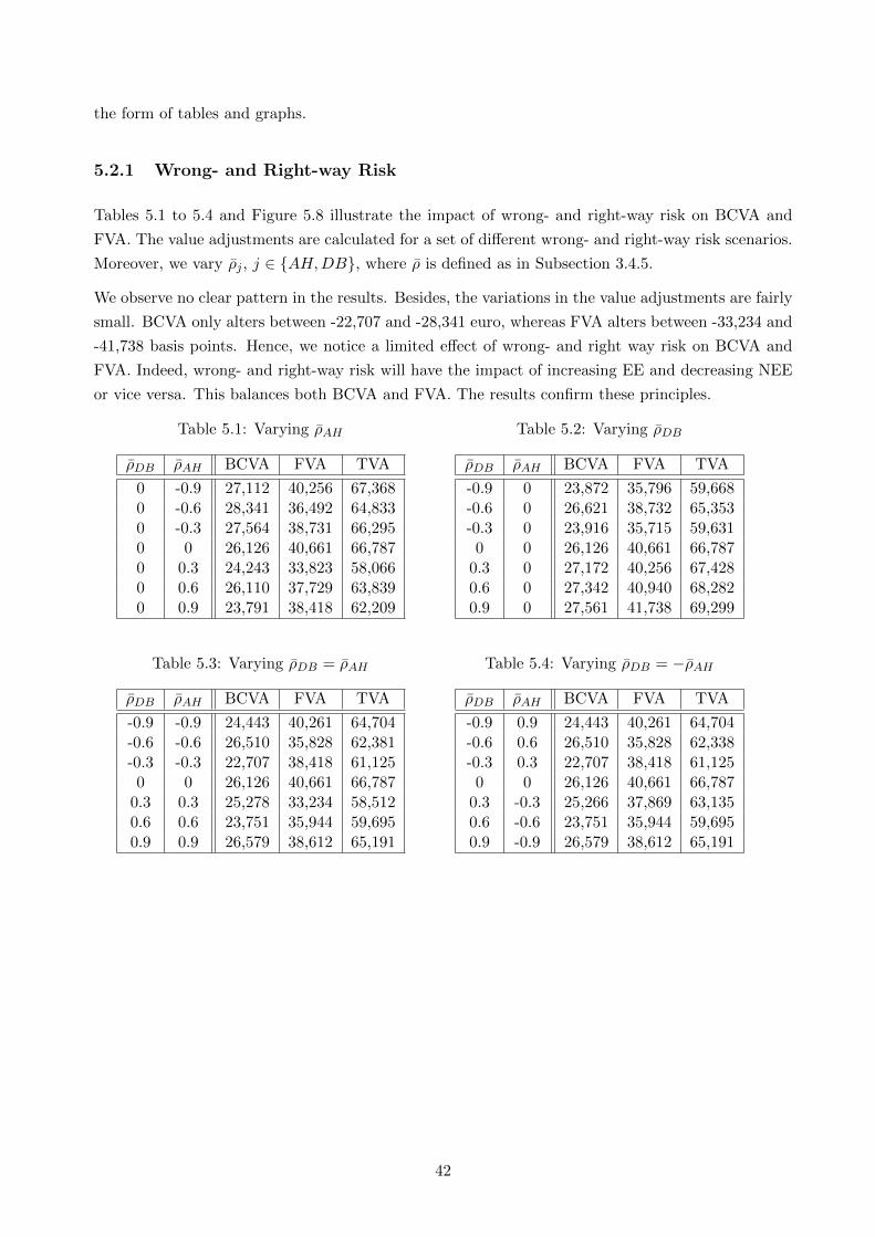
5.2.1 Wrong- and Right-way Risk
Tables 5.1 to 5.4 and Figure 5.8 illustrate the impact of wrong- and right-way risk on BCVA and
FVA. The value adjustments are calculated for a set of different wrong- and right-way risk scenarios.
Moreover, we vary ρj , j ∈ {AH,DB}, where ρ is defined as in Subsection 3.4.5.
We observe no clear pattern in the results. Besides, the variations in the value adjustments are fairly
small. BCVA only alters between -22,707 and -28,341 euro, whereas FVA alters between -33,234 and
-41,738 basis points. Hence, we notice a limited effect of wrong- and right way risk on BCVA and
FVA. Indeed, wrong- and right-way risk will have the impact of increasing EE and decreasing NEE
or vice versa. This balances both BCVA and FVA. The results confirm these principles.
Figure 5.10: Plot of the estimated value adjustments in the case we vary νDB = νAH , the x-axisdenotes the increase in both νDB and νAH .
45
Chapter 6
Conclusion
The main result of this thesis is an innovative framework for modelling funding value adjustment.
We motivated and examined this framework in the form of a case study considering a plain vanilla
interest rate swap. Nevertheless, the proposed framework for modelling funding value adjustment
can be applied to many different derivative products.
In general our FVA estimates are significant and quite sensitive to parameter dynamics. Moreover,
the impact of wrong- and right-way risk is found to be limited, whereas credit spread levels have
a structured effect on both BCVA and FVA. Besides, the often neglected impact of credit spread
volatility is found to be non negligible. Therefore there is a need to rigorously model these dynamical
features. We have chosen a G2++ model for interest rates, a CIR model for the Euribor-OIS spread,
a CIR++ model for credit spreads and a CIR model for net funding cost. We document our findings
in the form of tables and graphs.
Still, there are great opportunities to extent the modelling framework in future research. The aca-
demic field of FVA is far from discovered, hence plenty of extensions are possible. To start with,
one can model the dependence structure between funding spreads and credit spreads (i.e. wrong-way
funding risk). For example, a correlation between the treasury’s internal lending rate and the bank’s
credit spread can be considered: does the treasury’s internal lending rate rises as the creditworthiness
of the bank weakens? Besides, one can extend the modelling framework in order to calculate FVA
for netting sets or investigate the effect of different funding policies on FVA. Likewise, the impact on
FVA of different credit spread and interest rate models can be examined. Another extension would
be to implement discretization schemes that diminish districtization errors and give more accurate
estimations of BCVA and FVA. Lastly, one can introduce default correlation between entities by
making use of copulas.
It may be clear that the implementation of FVA is complex and that there is a great need for a
market practice regarding FVA. Indeed, the price of a derivative including FVA is different for each
entity since each entity has its own funding policy. Therefore, there is no law of one price regarding
derivatives pricing including funding risk and deals will be made through negotiations. Thus, FVA
cannot be estimated correctly based on market observable quantities.
International Financial Reporting Standards 13 already forces banks and other derivative dealers to
46
incorporate CVA and DVA. However, it may be clear that similar obligatory accounting practices
are inapplicable to FVA in the current market environment. The Basel Committee on Banking
Supervision can consider to force (big) bank to make their internal lending rates public. This could
be a first step towards a market observable FVA and may foster the commencement of a market
practice regarding FVA. Likewise, the origination of an industry average of the relevant treasury’s
internal lending rate of big banks could also be a possibility.
This thesis confirms the tremendous impact of the global credit crisis on the key concepts underlying
the valuation of derivatives contracts. As a result, the valuation of derivatives contracts is much
debated today making even the valuation of the simplest derivatives contracts a challenging task.
This shows how significant the effect of post-crisis realities such as the Libor-OIS spread can be.
47
Appendix A
Market Data
Figure A.1: Market data of the 3 month Euribor and Eonia rate in respectively the right and leftfigure (obtained from Bloomberg on April 30, 2014) .
48
Figure A.2: Market at-the-money swaption volatilities, obtained from Bloomberg on April 30, 2014.Each column indicates the tenor of the swaption, whereas each row denotes the maturity of theswaption.
Figure A.3: Market CDS curves of Deutsche Bank AG and Koninklijke Ahold NV in respectively theleft and right figure (CDS spreads are in basispoints). The data is obtained from Bloomberg on April30, 2014.
Figure A.4: Bond yield curve of Deutsche Bank AG, built with senior unsecured fixed rate bondsissued by Deutsche Bank AG (obtained from Bloomberg on April 30, 2014).
49
References
Bianchetti, M. (2010). Two curves , one price. Risk , 74–80.
Black, F., & Scholes, M. (1973). The Pricing of Options and Corporate Liabilities (Vol. 81). doi:
10.1086/260062
Brigo, D., Buescu, C., & Morini, M. (2011). arXiv : 1106 . 3496v1 [ q-fin . PR ] 17 Jun 2011. , 1–14.
Brigo, D., Liu, Q., Pallavicini, A., & Sloth, D. (2014). Nonlinear Valuation Under Collateral, Credit
Risk and Funding Costs: A Numerical Case Study Extending Black-Scholes. Handbook in Fixed-
Income Securities. Retrieved from http://papers.ssrn.com/sol3/papers.cfm?abstract id=
2430696
Brigo, D., & Mercurio, F. (2006). Interest rate models-theory and practice: with smile, inflation and
credit (Vol. 82).
Brigo, D., Morini, M., & Pallavicini, A. (2013). Counterparty Credit Risk, Collateral and Funding:
With Pricing Cases for All Asset Classes.
Cameron, M. (2014). The black art of FVA, part II: Conditioning chaos. Risk magazine. Re-
trieved from http://www.risk.net/risk-magazine/feature/2335564/the-black-art-of-fva
-part-ii-conditioning-chaos
Carver, L. (2012). Quant Congress Europe: FVA ends Platonic price, says Brigo. Risk, (October).
Retrieved from http://www.risk.net/risk-magazine/news/2216253/quant-congress-europe
-fva-ends-platonic-price-says-brigo
Castagna, A. (2012). Yes, FVA is a Cost for Derivatives Desks. iasonltd.com, 1–15. Retrieved from