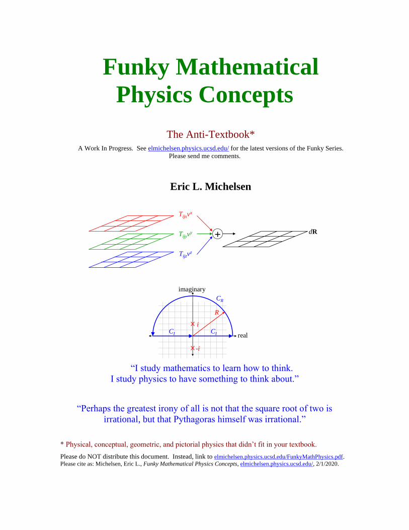
Page 1
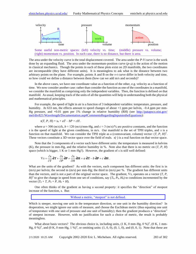
Funky Mathematical
Physics Concepts
The Anti-Textbook*
A Work In Progress. See elmichelsen.physics.ucsd.edu/ for the latest versions of the Funky Series.
Please send me comments.
Eric L. Michelsen
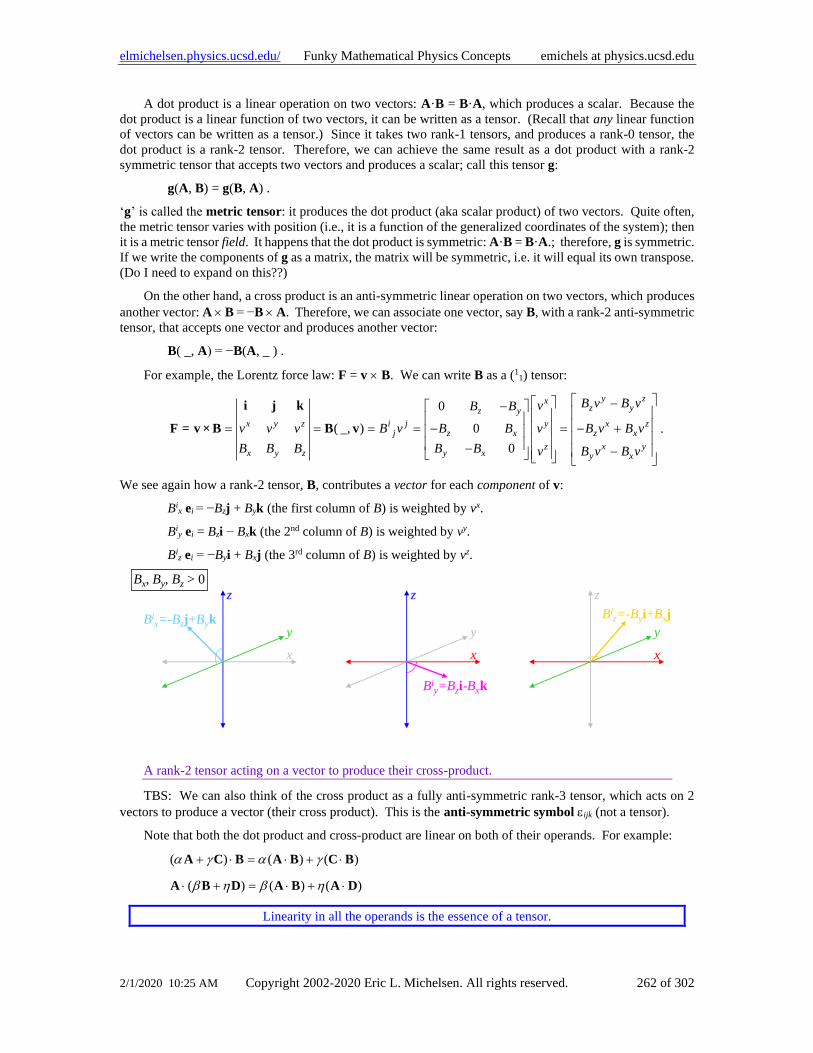
Tijxvx
Tijyvy
Tijzvz
+ dR
real
imaginary
CI
CR
i
-i
R
CI
“I study mathematics to learn how to think.
I study physics to have something to think about.”
“Perhaps the greatest irony of all is not that the square root of two is
irrational, but that Pythagoras himself was irrational.”
* Physical, conceptual, geometric, and pictorial physics that didn’t fit in your textbook.
Please do NOT distribute this document. Instead, link to elmichelsen.physics.ucsd.edu/FunkyMathPhysics.pdf. Please cite as: Michelsen, Eric L., Funky Mathematical Physics Concepts, elmichelsen.physics.ucsd.edu/, 2/1/2020.
Page 2
elmichelsen.physics.ucsd.edu/ Funky Mathematical Physics Concepts emichels at physics.ucsd.edu
2/1/2020 10:25 AM Copyright 2002-2020 Eric L. Michelsen. All rights reserved. 2 of 302
2006 values from NIST. For more physical constants, see http://physics.nist.gov/cuu/Constants/ .
Speed of light in vacuum c = 299 792 458 m s–1 (exact)
Boltzmann constant k = 1.380 6504(24) x 10–23 J K–1
Stefan-Boltzmann constant σ = 5.670 400(40) x 10–8 W m–2 K–4
Relative standard uncertainty ±7.0 x 10⁻⁶
Avogadro constant NA, L = 6.022 141 79(30) x 1023 mol–1
Relative standard uncertainty ±5.0 x 10⁻⁸
Molar gas constant R = 8.314 472(15) J mol-1 K-1
Electron mass me = 9.109 382 15(45) x 10–31 kg
Proton mass mp = 1.672 621 637(83) x 10–27 kg
Proton/electron mass ratio mp/me = 1836.152 672 47(80)
Elementary charge e = 1.602 176 487(40) x 10–19 C
Electron g-factor ge = –2.002 319 304 3622(15)
Proton g-factor gp = 5.585 694 713(46)
Neutron g-factor gN = –3.826 085 45(90)
Muon mass mμ = 1.883 531 30(11) x 10–28 kg
Inverse fine structure constant –1 = 137.035 999 679(94)
Planck constant h = 6.626 068 96(33) x 10–34 J s
Planck constant over 2π ħ = 1.054 571 628(53) x 10–34 J s
Bohr radius a0 = 0.529 177 208 59(36) x 10–10 m
Bohr magneton μB = 927.400 915(23) x 10–26 J T–1
Reviews
“... most excellent tensor paper.... I feel I have come to a deep and abiding understanding of relativistic
tensors.... The best explanation of tensors seen anywhere!” -- physics graduate student
Page 3
elmichelsen.physics.ucsd.edu/ Funky Mathematical Physics Concepts emichels at physics.ucsd.edu
2/1/2020 10:25 AM Copyright 2002-2020 Eric L. Michelsen. All rights reserved. 3 of 302
Contents
1 Introduction ........................................................................................................................................... 9 Mathematical Physics, or Physical Mathematics? ............................................................................ 9 Why Physicists and Mathematicians Argue ..................................................................................... 9 Why Funky? ..................................................................................................................................... 9 How to Use This Document ............................................................................................................. 9 Thank You .......................................................................................................................................10 Scope ...............................................................................................................................................10 Notation ...........................................................................................................................................10
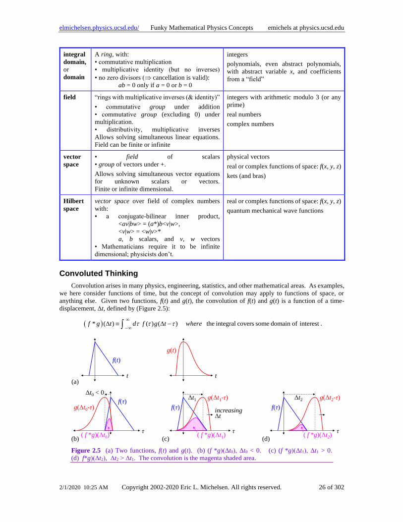
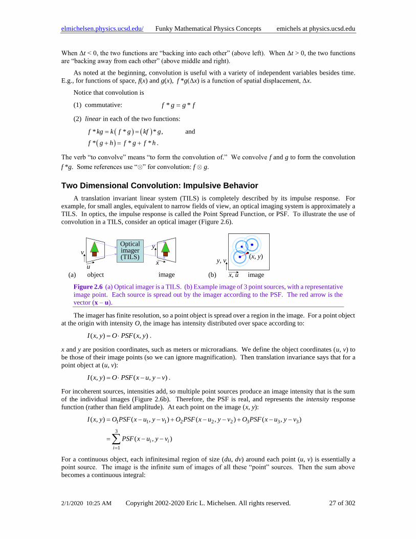
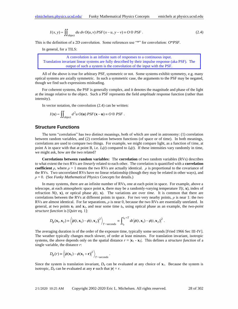
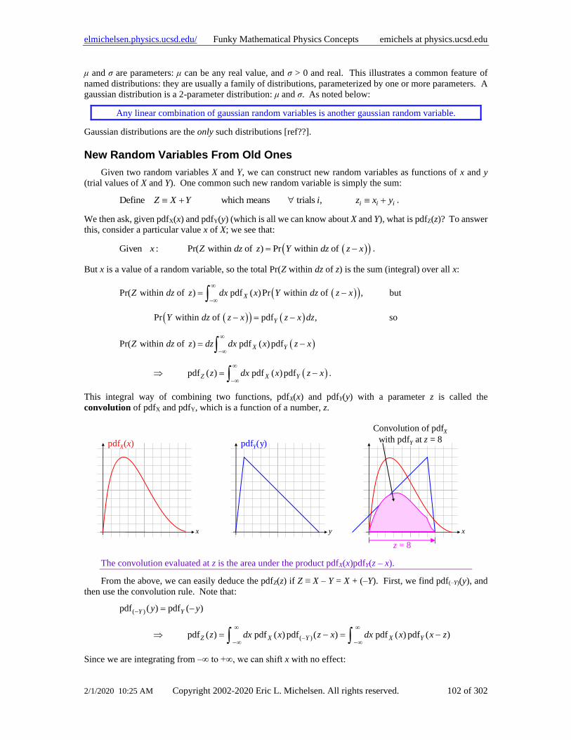
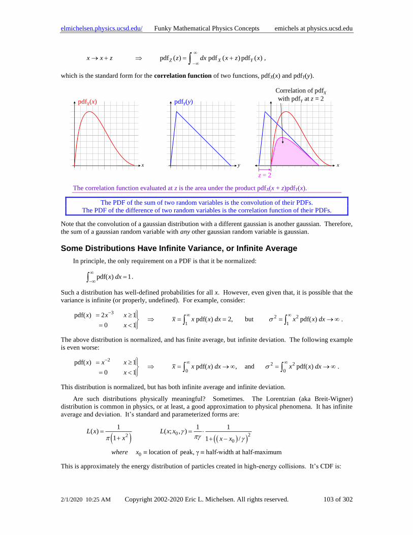
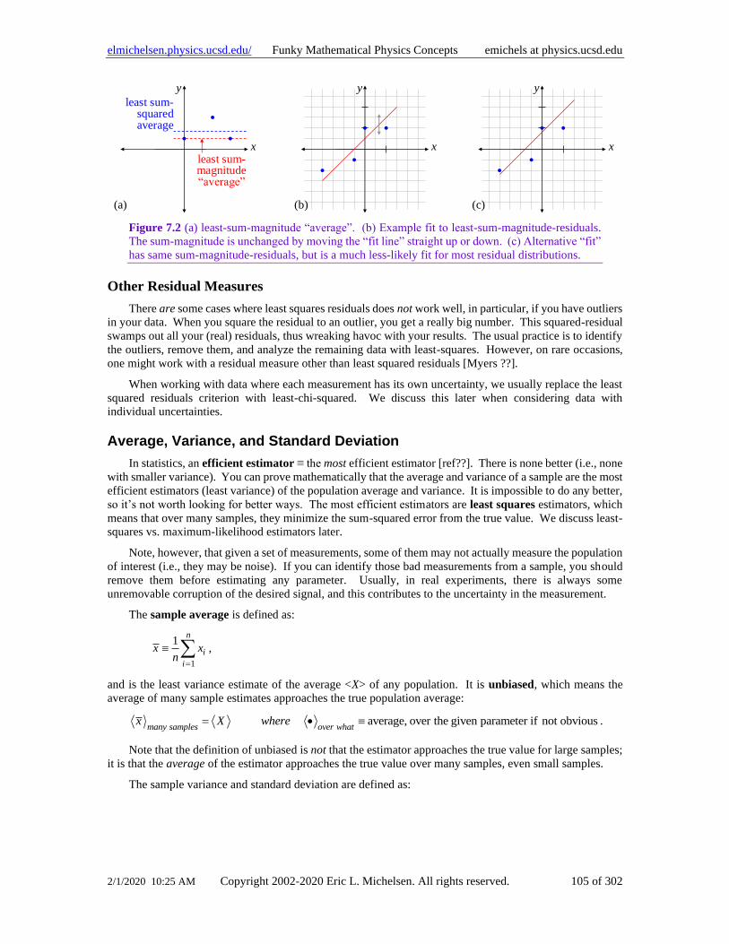
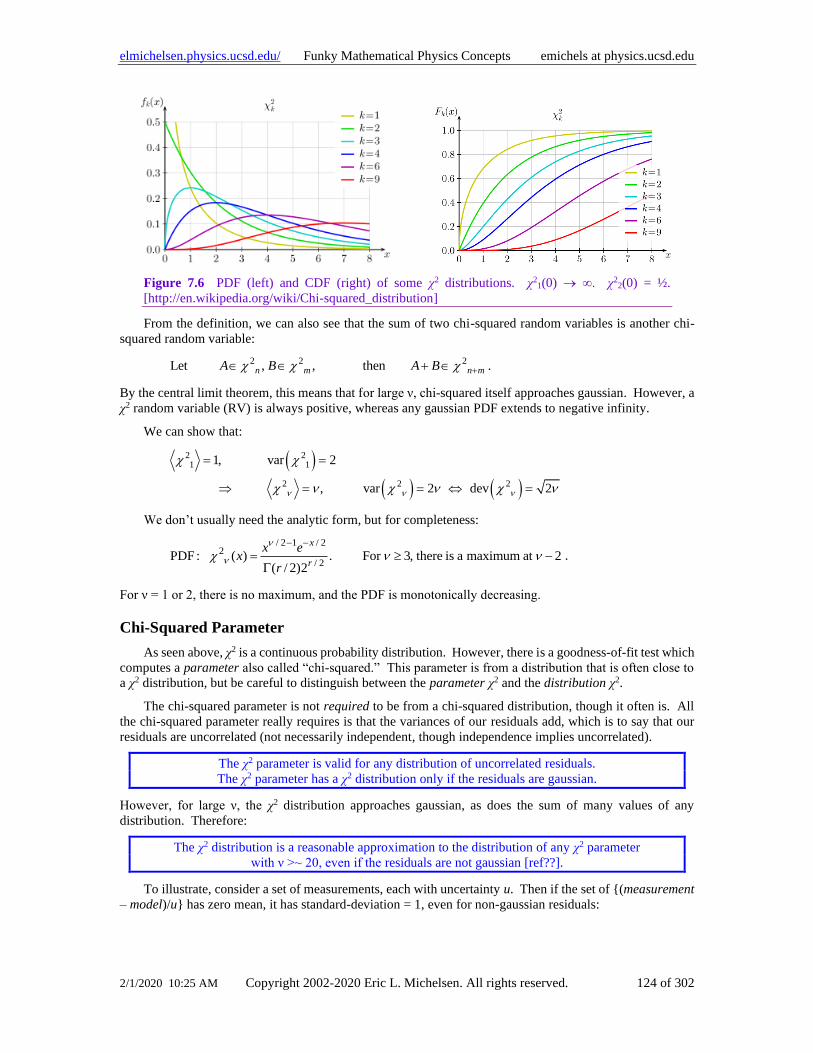
2 Random Short Topics ..........................................................................................................................13 I Always Lie ....................................................................................................................................13 What’s Hyperbolic About Hyperbolic Sine? ...................................................................................13 Basic Calculus You May Not Know ...............................................................................................15 The Product Rule.............................................................................................................................16 Integration By Pictures ....................................................................................................................16 Theoretical Importance of IBP ........................................................................................................20 Delta Function Surprise: Coordinates Matter ..................................................................................20 Spherical Harmonics Are Not Harmonics .......................................................................................22 The Binomial Theorem for Negative and Fractional Exponents .....................................................23 When Does a Divergent Series Converge? .....................................................................................24 Algebra Family Tree .......................................................................................................................25 Convoluted Thinking ......................................................................................................................26 Two Dimensional Convolution: Impulsive Behavior ......................................................................27 Structure Functions .........................................................................................................................28 Correlation Functions ......................................................................................................................29
3 Vectors ...................................................................................................................................................30 Small Changes to Vectors ...............................................................................................................30 Why (r, θ, ) Are Not the Components of a Vector ........................................................................30 Laplacian’s Place ............................................................................................................................31 Vector Dot Grad Vector ..................................................................................................................39
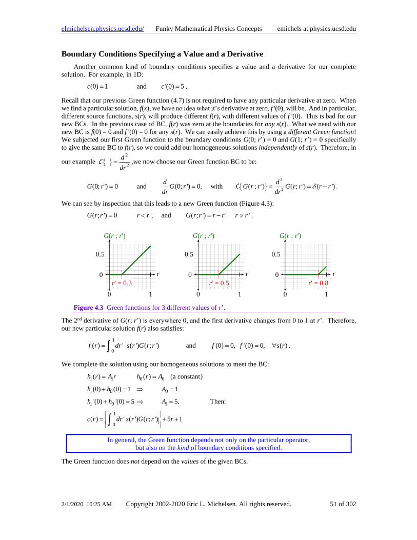
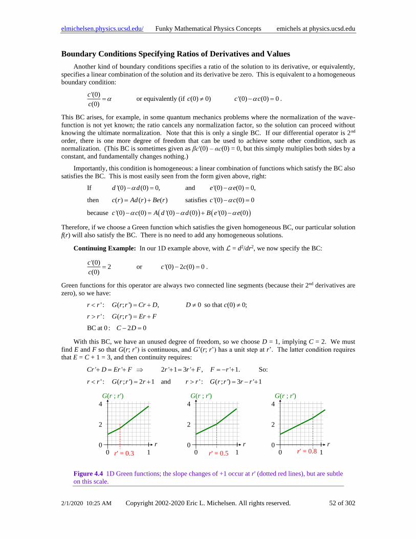
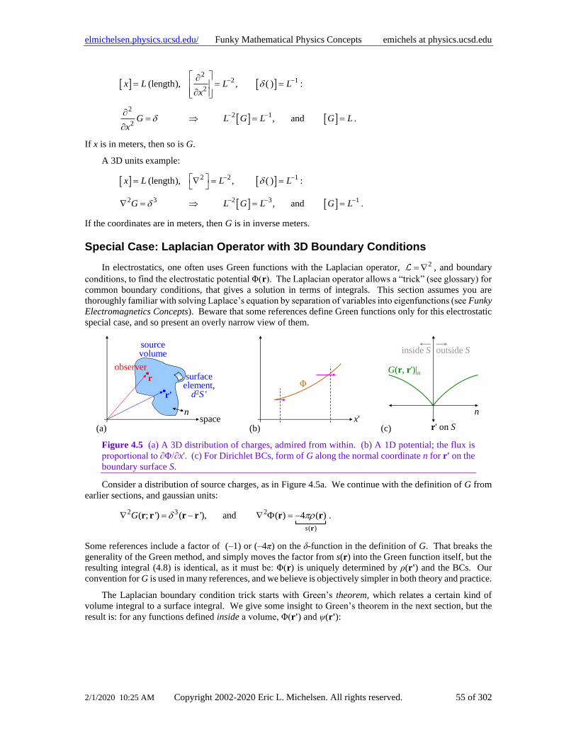
4 Green Functions ...................................................................................................................................41 The Big Idea ....................................................................................................................................41 Boundary Conditions on Green Functions ......................................................................................46 Introduction to Boundary Conditions ..............................................................................................46 One Dimensional Boundary Conditions ..........................................................................................47 2D?? and 3D Green Functions ........................................................................................................53 Green Functions Don’t Separate .....................................................................................................53 Green Units .....................................................................................................................................54 Special Case: Laplacian Operator with 3D Boundary Conditions ..................................................55 Desultory Green Topics ..................................................................................................................58 Fourier Series Method for Green Functions ....................................................................................58 Green-Like Methods: The Born Approximation .............................................................................61
5 Complex Analytic Functions ...............................................................................................................63 Residues ..........................................................................................................................................64 Contour Integrals .............................................................................................................................65 Evaluating Integrals ........................................................................................................................65 Choosing the Right Path: Which Contour? .....................................................................................68 Evaluating Infinite Sums .................................................................................................................73 Multi-valued Functions ...................................................................................................................75
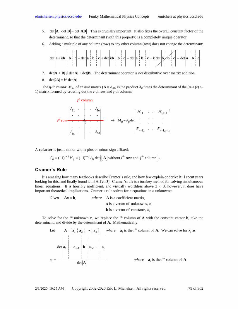
6 Conceptual Linear Algebra .................................................................................................................77 Matrix Multiplication ......................................................................................................................77 Determinants ...................................................................................................................................78
Page 4
elmichelsen.physics.ucsd.edu/ Funky Mathematical Physics Concepts emichels at physics.ucsd.edu
2/1/2020 10:25 AM Copyright 2002-2020 Eric L. Michelsen. All rights reserved. 4 of 302
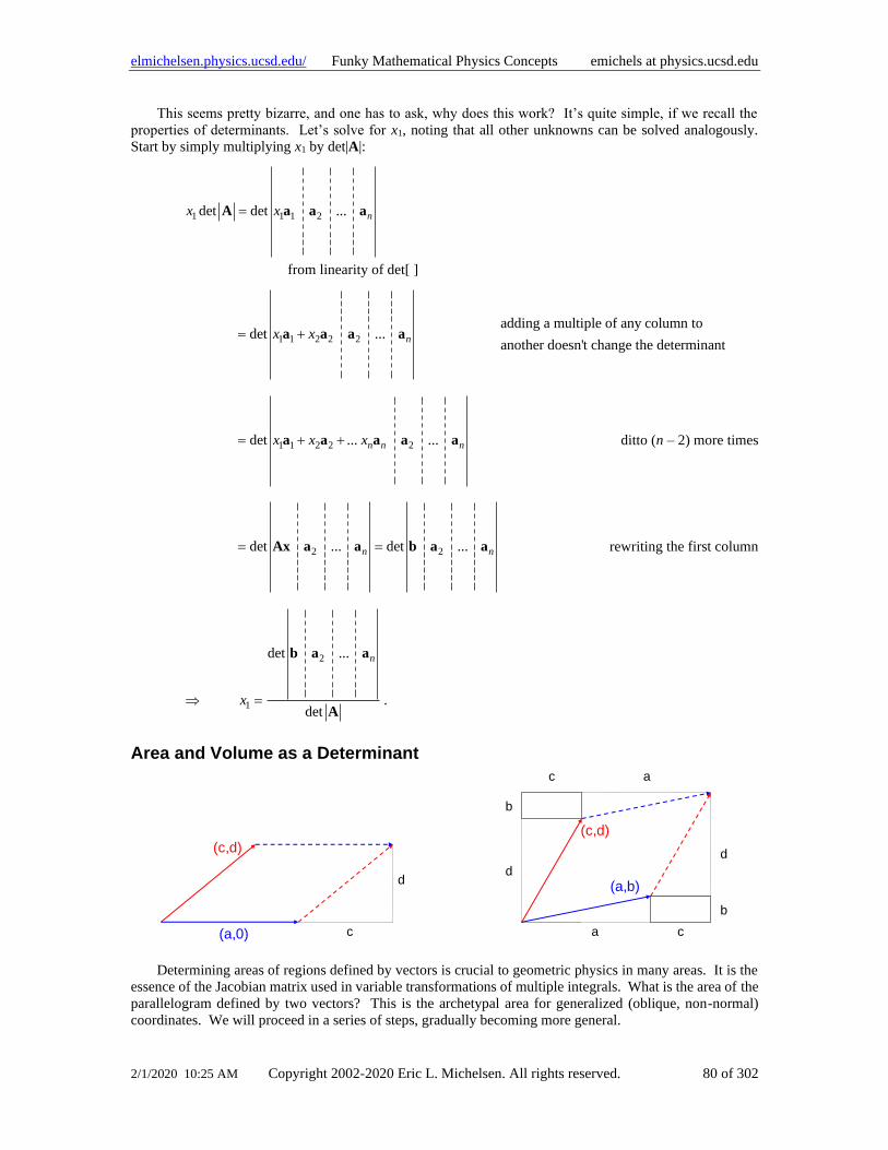
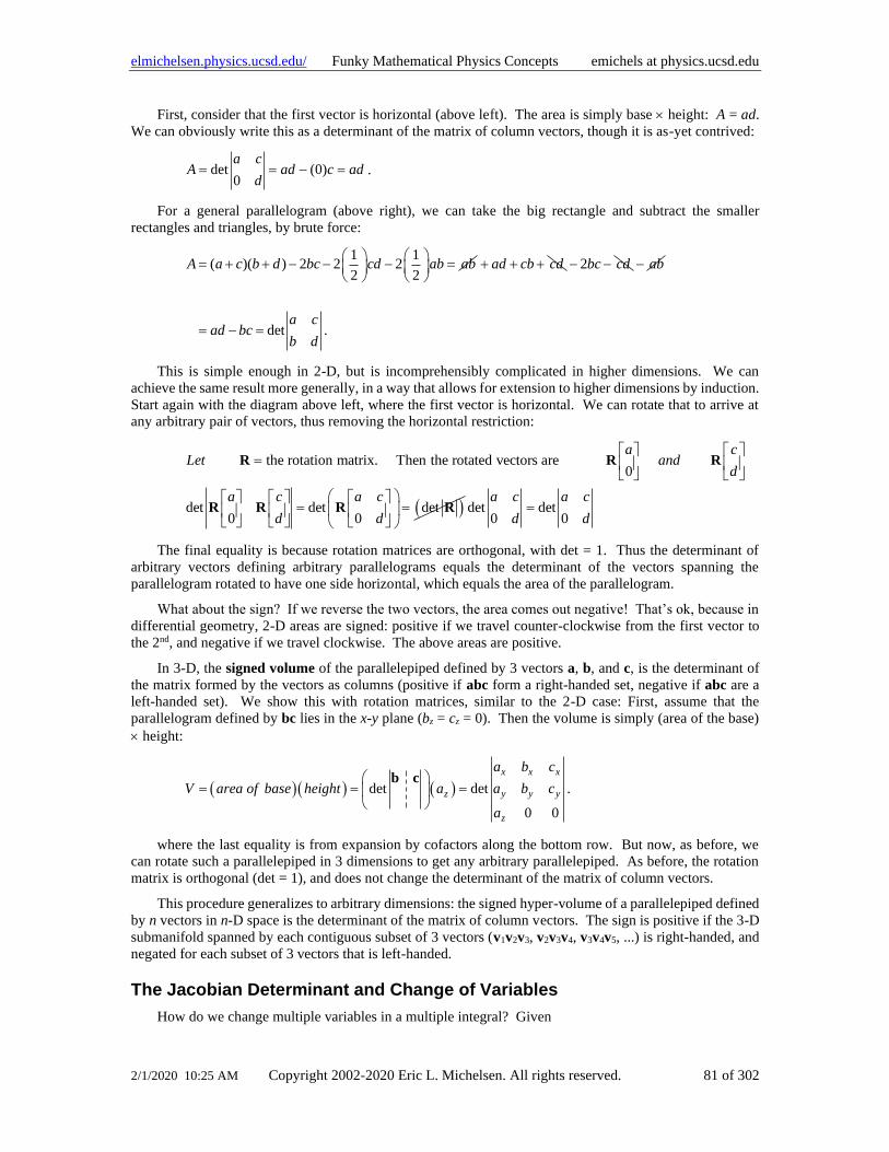
Cramer’s Rule .................................................................................................................................79 Area and Volume as a Determinant ................................................................................................80 The Jacobian Determinant and Change of Variables ......................................................................81 Expansion by Cofactors ..................................................................................................................83 Proof That the Determinant Is Unique ............................................................................................85 Getting Determined .........................................................................................................................86 Advanced Matrices ..........................................................................................................................87 Getting to Home Basis ....................................................................................................................87 Diagonalizing a Self-Adjoint Matrix ...............................................................................................88 Contraction of Matrices ...................................................................................................................90 Trace of a Product of Matrices ........................................................................................................90 Linear Algebra Briefs ......................................................................................................................91
7 Probability, Statistics, and Data Analysis ..........................................................................................92 Probability and Random Variables .....................................................................................................92
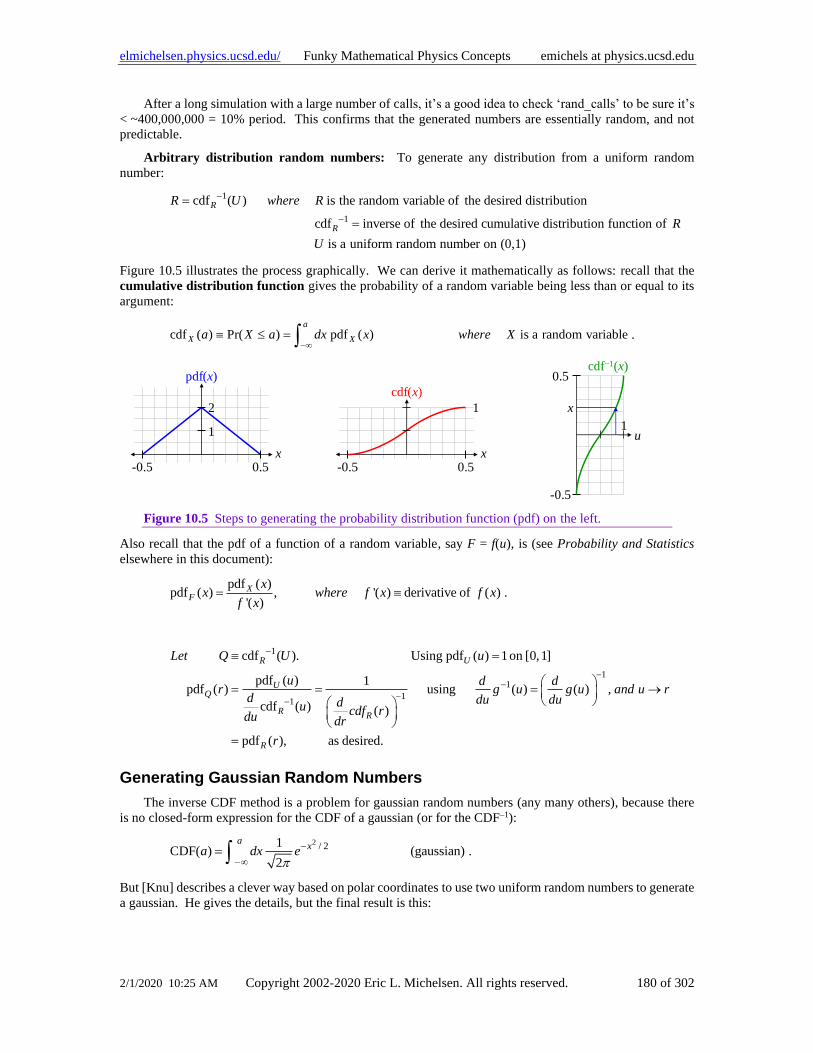
Precise Statement of the Question Is Critical ..................................................................................93 How to Lie With Statistics ..............................................................................................................94 Choosing Wisely: An Informative Puzzle .......................................................................................94 Multiple Events ...............................................................................................................................95 Combining Probabilities ..................................................................................................................96 To B, or To Not B? .........................................................................................................................98 Continuous Random Variables and Distributions ...........................................................................99
Populations .......................................................................................................................................100 Population Variance ......................................................................................................................101 Population Standard Deviation ......................................................................................................101 New Random Variables From Old Ones .......................................................................................102 Some Distributions Have Infinite Variance, or Infinite Average ..................................................103
Samples and Parameter Estimation ...................................................................................................104 Why Do We Use Least Squares, and Least Chi-Squared (χ2)? .....................................................104 Average, Variance, and Standard Deviation .................................................................................105 Functions of Random Variables ....................................................................................................108 Statistically Speaking: What Is The Significance of This? ...........................................................109 Predictive Power: Another Way to Be Significant, but Not Important .........................................112 Unbiased vs. Maximum-Likelihood Estimators ............................................................................112 Correlation and Dependence .........................................................................................................114 Independent Random Variables are Uncorrelated .........................................................................115 r You Serious? ..............................................................................................................................116
Statistical Analysis Algebra ..............................................................................................................117 The Average of a Sum: Easy? .......................................................................................................117 The Average of a Product..............................................................................................................117 Variance of a Sum .........................................................................................................................118 Covariance Revisited ....................................................................................................................118 Capabilities and Limits of the Sample Variance ...........................................................................118 How to Do Statistical Analysis Wrong, and How to Fix It ...........................................................121
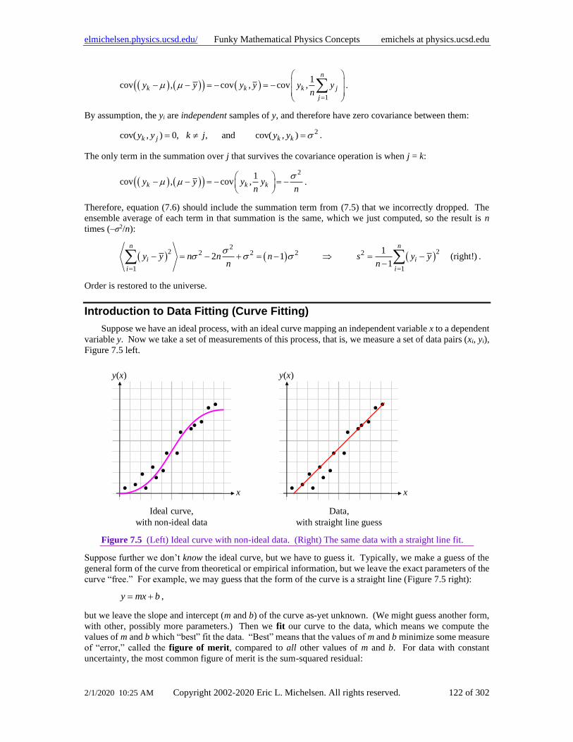
Introduction to Data Fitting (Curve Fitting) .....................................................................................122 Goodness of Fit .............................................................................................................................123
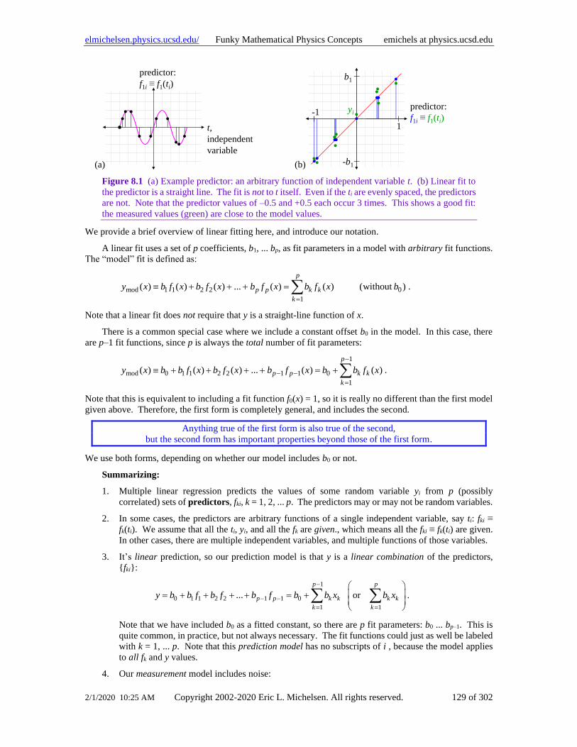
8 Linear Regression ...............................................................................................................................128 Review of Multiple Linear Regression .........................................................................................128 We Fit to the Predictors, Not the Independent Variable ................................................................128
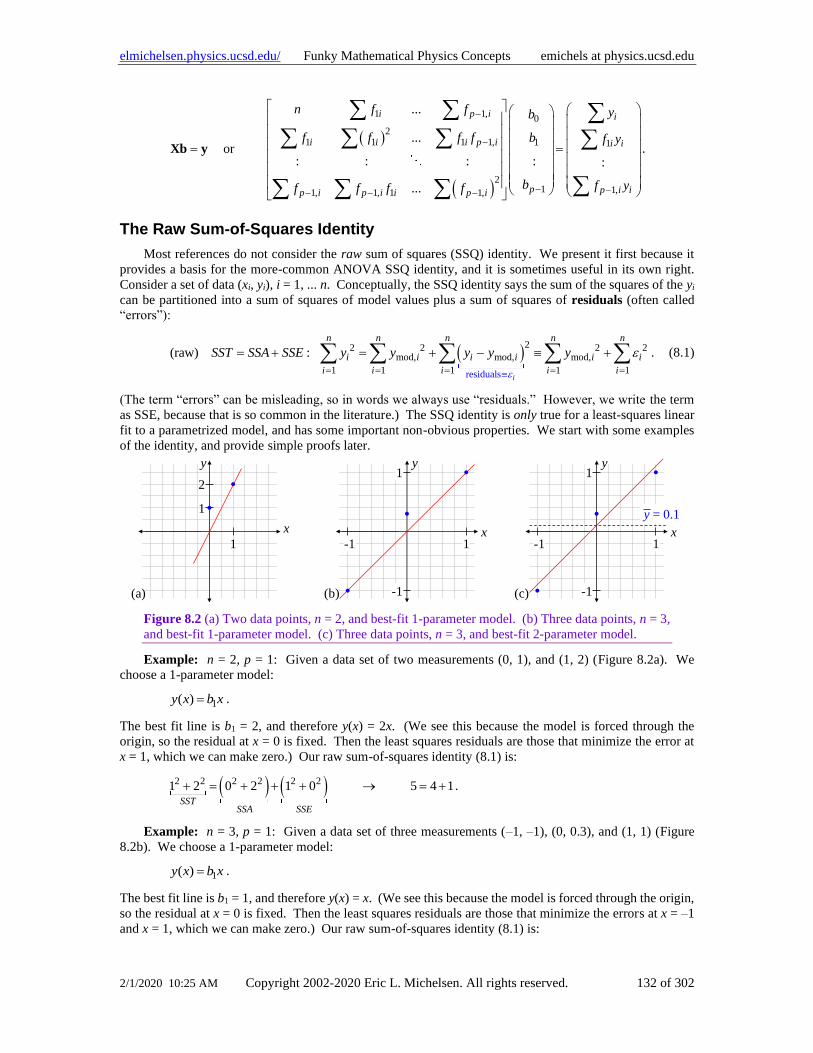
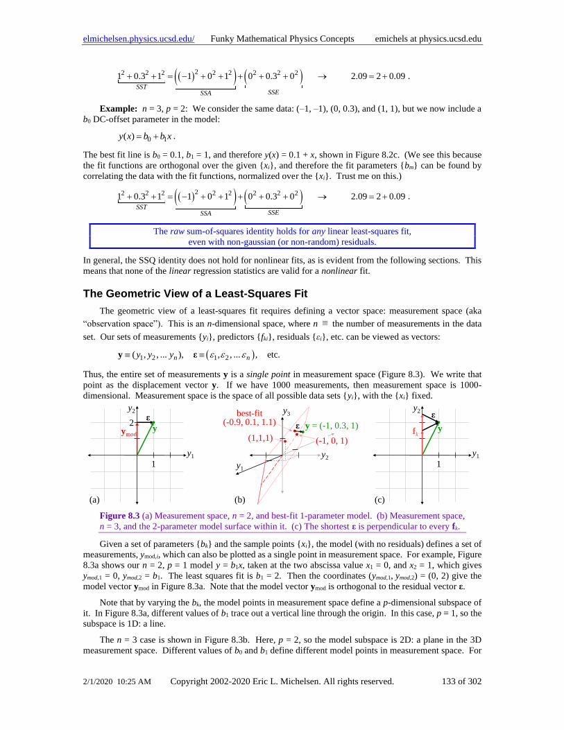
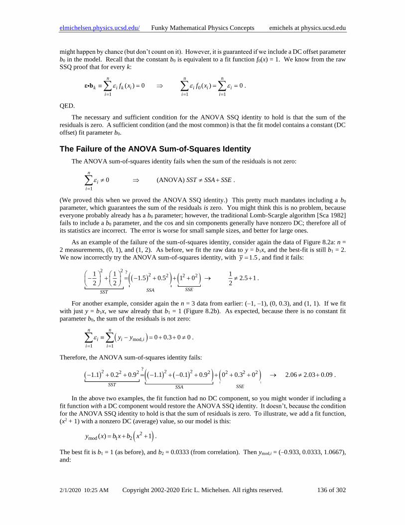
The Sum-of-Squares Identity ............................................................................................................131 Homoskedastic Case: All Measurements Have the Same Uncertainty .........................................131 The Raw Sum-of-Squares Identity ................................................................................................132 The Geometric View of a Least-Squares Fit .................................................................................133 Algebra and Geometry of the Sum-of-Squares Identity ................................................................134 The ANOVA Sum-of-Squares Identity .........................................................................................135 The Failure of the ANOVA Sum-of-Squares Identity ...................................................................136
Page 5
elmichelsen.physics.ucsd.edu/ Funky Mathematical Physics Concepts emichels at physics.ucsd.edu
2/1/2020 10:25 AM Copyright 2002-2020 Eric L. Michelsen. All rights reserved. 5 of 302
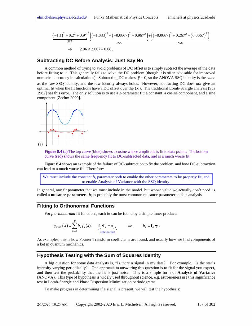
Subtracting DC Before Analysis: Just Say No ..............................................................................137 Fitting to Orthonormal Functions .....................................................................................................137 Hypothesis Testing with the Sum of Squares Identity ......................................................................137
Introduction to Analysis of Variance (ANOVA) ..........................................................................138 The Temperature of Liberty ..........................................................................................................139 The F-test: The Decider for Zero Mean Gaussian Noise ...............................................................142 Coefficient of Determination and Correlation Coefficient ............................................................143
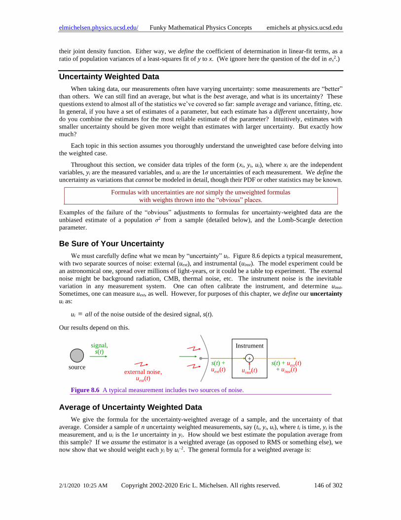
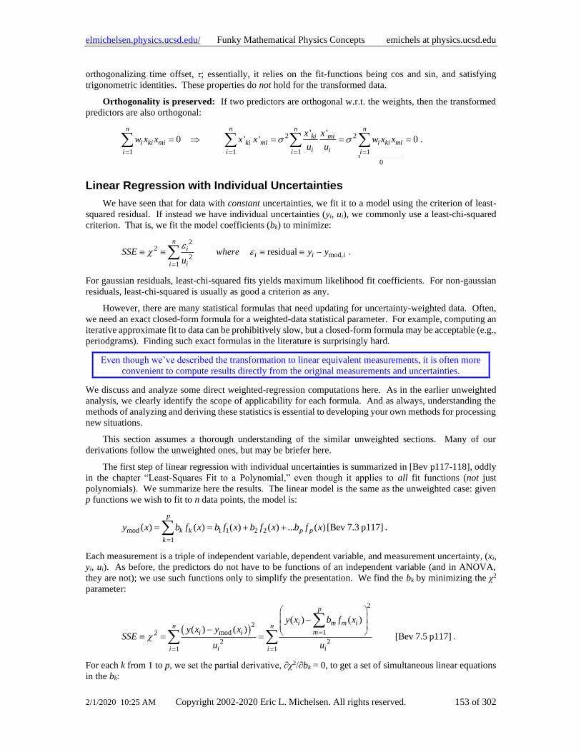
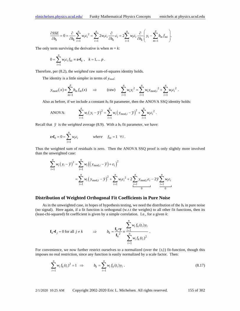
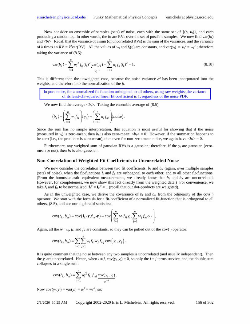
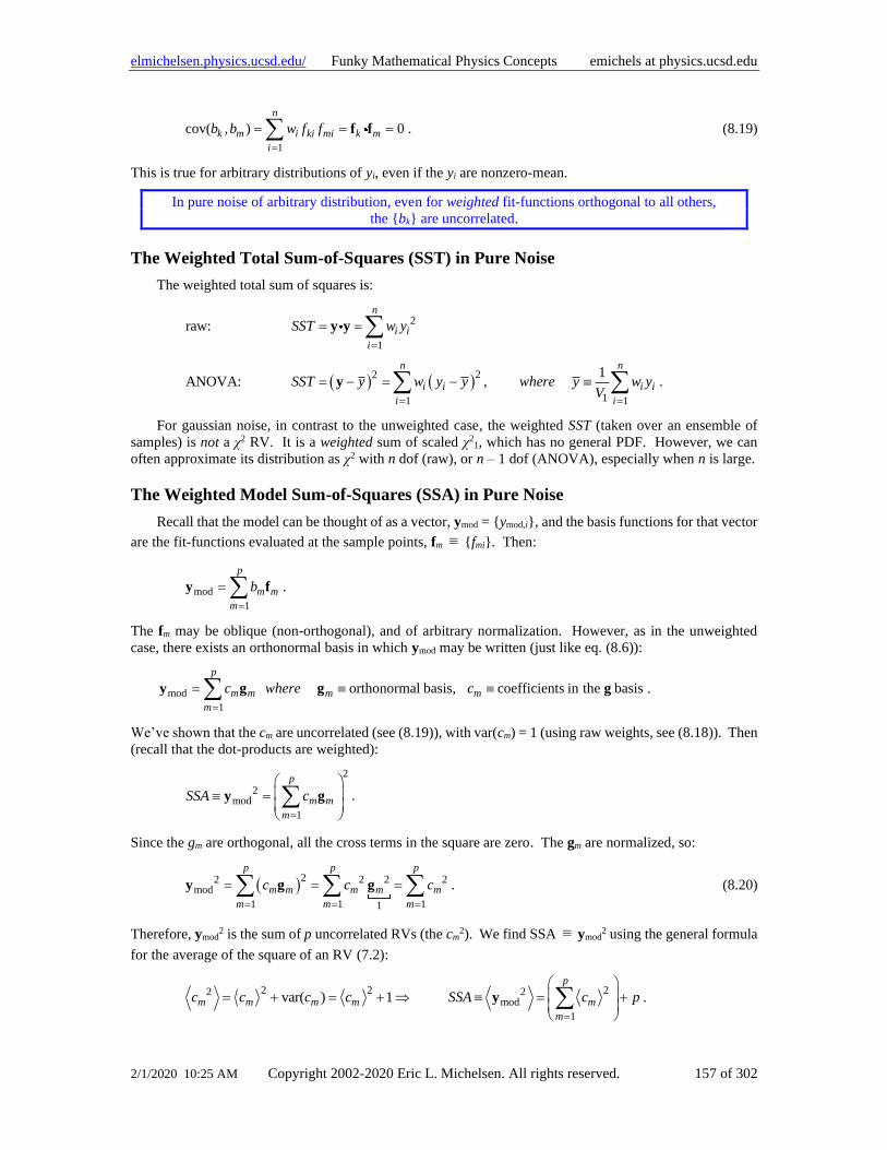
Uncertainty Weighted Data ..............................................................................................................146 Be Sure of Your Uncertainty .........................................................................................................146 Average of Uncertainty Weighted Data ........................................................................................146 Variance and Standard Deviation of Uncertainty Weighted Data .................................................148 Normalized weights ......................................................................................................................150 Numerically Convenient Weights .................................................................................................151 Transformation to Equivalent Homoskedastic Measurements ......................................................151 Linear Regression with Individual Uncertainties ..........................................................................153 Linear Regression With Uncertainties and the Sum-of-Squares Identity ......................................154 Hypothesis Testing a Model in Linear Regression with Uncertainties .........................................158
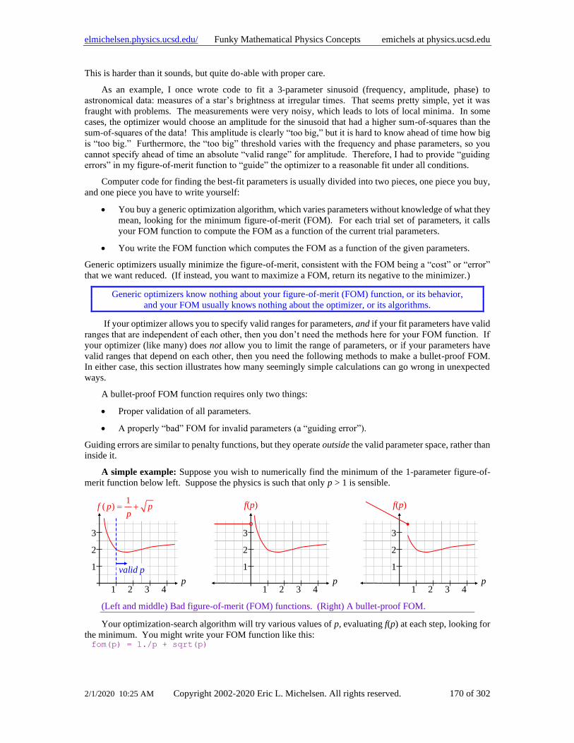
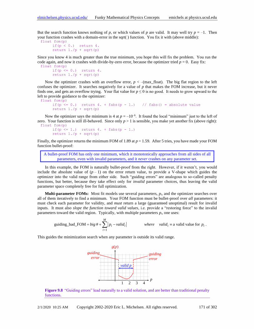
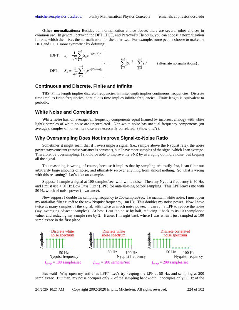
9 Practical Considerations for Data Analysis .....................................................................................159 Rules of Thumb .............................................................................................................................159 Signal to Noise Ratio (SNR) .........................................................................................................159 Computing SNR From Data ..........................................................................................................160 Spectral Method of Estimating SNR .............................................................................................161 Fitting Models To Histograms (Binned Data) ...............................................................................162 Reducing the Effect of Noise ........................................................................................................165 Data With a Hard Cutoff: When Zero Just Isn’t Enough ..............................................................167 Filtering and Data Processing for Equally Spaced Samples ..........................................................168 Finite Impulse Response Filters (aka Rolling Filters) and Boxcars ..............................................168 Use Smooth Filters (not Boxcars) .................................................................................................169 Guidance Counselor: Computer Code to Fit Data .........................................................................169
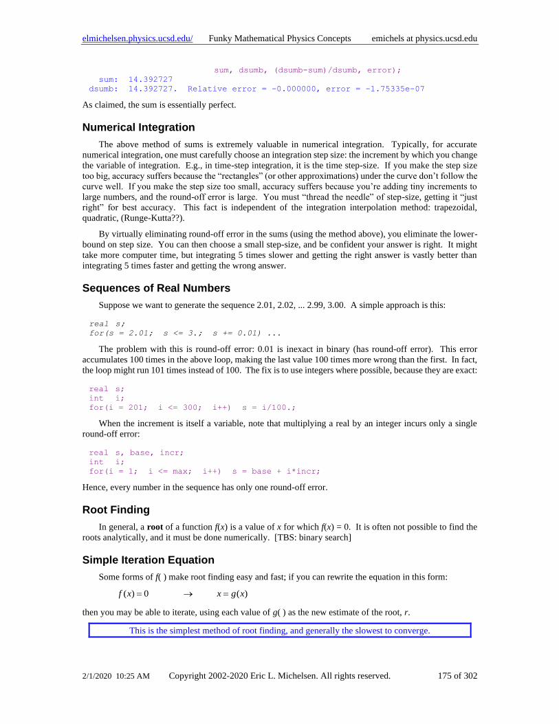
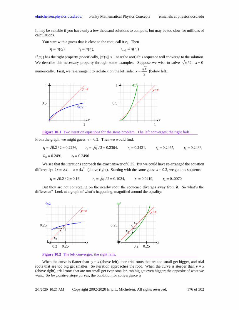
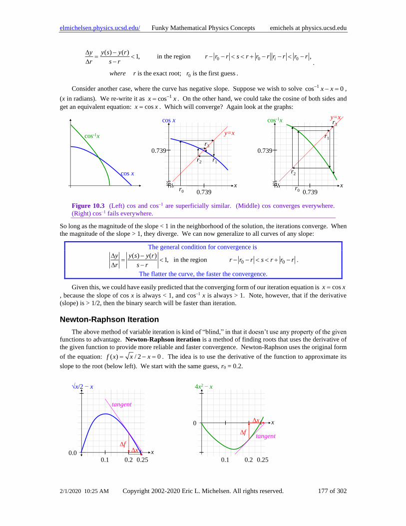
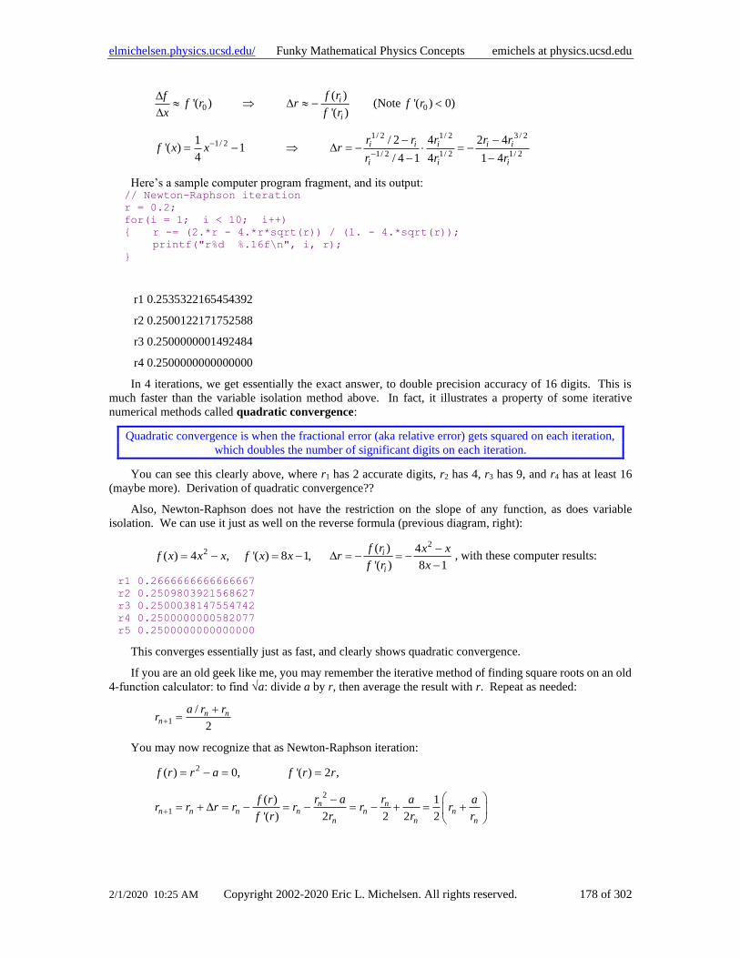
10 Numerical Analysis ............................................................................................................................173 Round-Off Error, And How to Reduce It ......................................................................................173 How To Extend Precision In Sums Without Using Higher Precision Variables ...........................174 Numerical Integration ...................................................................................................................175 Sequences of Real Numbers ..........................................................................................................175 Root Finding .................................................................................................................................175 Simple Iteration Equation..............................................................................................................175 Newton-Raphson Iteration ............................................................................................................177 Pseudo-Random Numbers .............................................................................................................179 Generating Gaussian Random Numbers .......................................................................................180 Generating Poisson Random Numbers..........................................................................................181 Generating Weirder Random Numbers .........................................................................................182 Exact Polynomial Fits ...................................................................................................................182 Two’s Complement Arithmetic .....................................................................................................184 How Many Digits Do I Get, 6 or 9? ..............................................................................................185 How many digits do I need? ..........................................................................................................186 How Far Can I Go? .......................................................................................................................186 IEEE Floating Point Formats And Concepts .................................................................................186 Precision in Decimal Representation ............................................................................................194 Underflow .....................................................................................................................................195
11 Scientific Programming: Discovering Efficiency .............................................................................201 Software Development Efficiency ................................................................................................201 Some Do s and Don’t s ..................................................................................................................201 Considerations on Development Efficiency and Languages .........................................................202 Sophistication Follows Function ...................................................................................................202
Page 6
elmichelsen.physics.ucsd.edu/ Funky Mathematical Physics Concepts emichels at physics.ucsd.edu
2/1/2020 10:25 AM Copyright 2002-2020 Eric L. Michelsen. All rights reserved. 6 of 302
Engineering vs. Programming .......................................................................................................202 Object Oriented Programming ......................................................................................................203 The Best of Times, the Worst of Times: Run-time Efficiency ......................................................204 Example Using Matrix Addition ...................................................................................................205 Memory Consumption vs. Run Time ............................................................................................209 Cache Withdrawal: Making the Most of Reference Locality ........................................................211 Data Structures for Efficient Cache Use .......................................................................................212 Algorithms for Efficient Cache Use ..............................................................................................212 Cache Optimization Summary ......................................................................................................213 Page Locality .................................................................................................................................213 Considerations on Run-Time Efficiency and Languages ..............................................................214
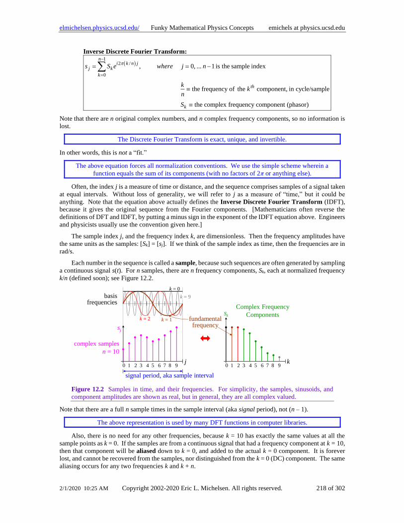
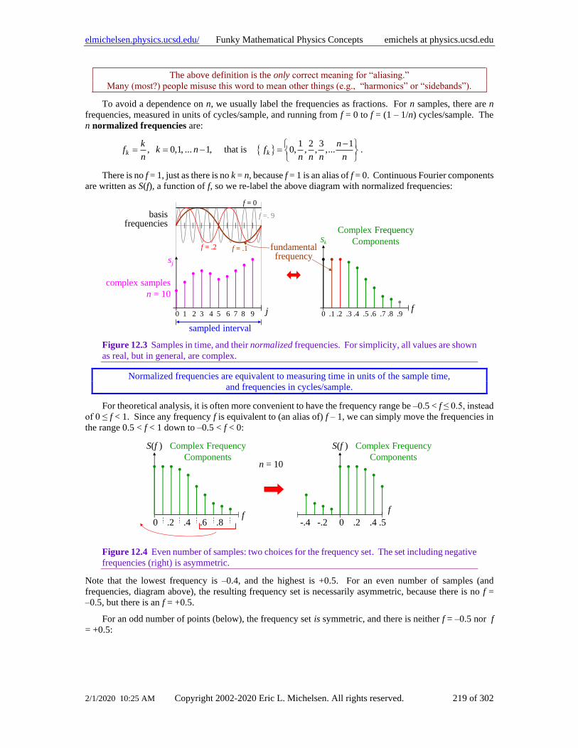
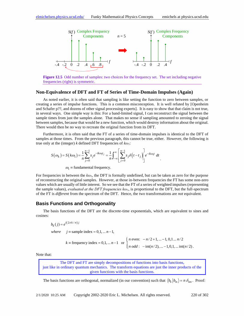
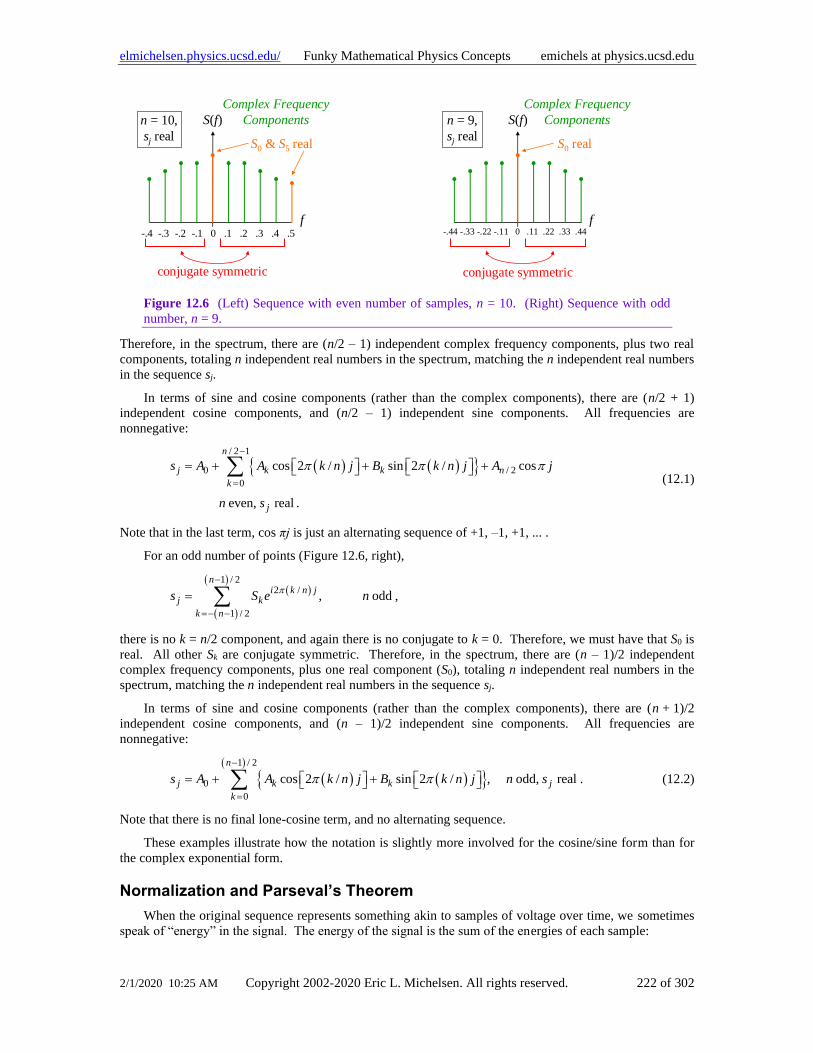
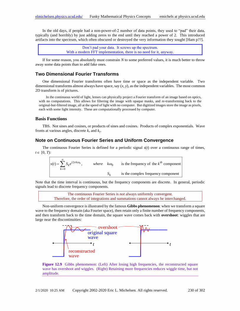
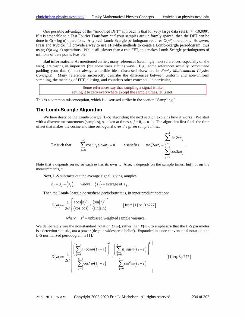
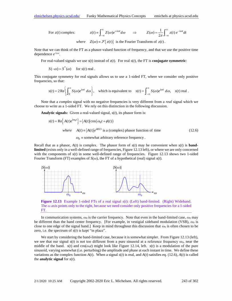
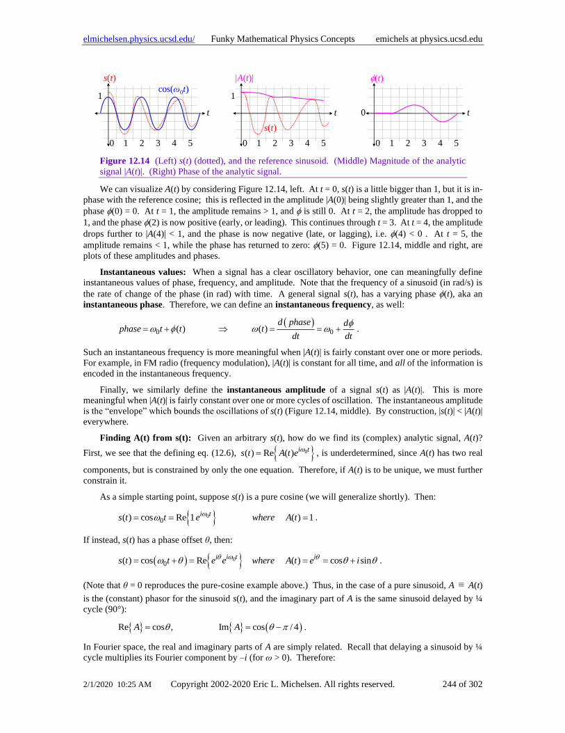
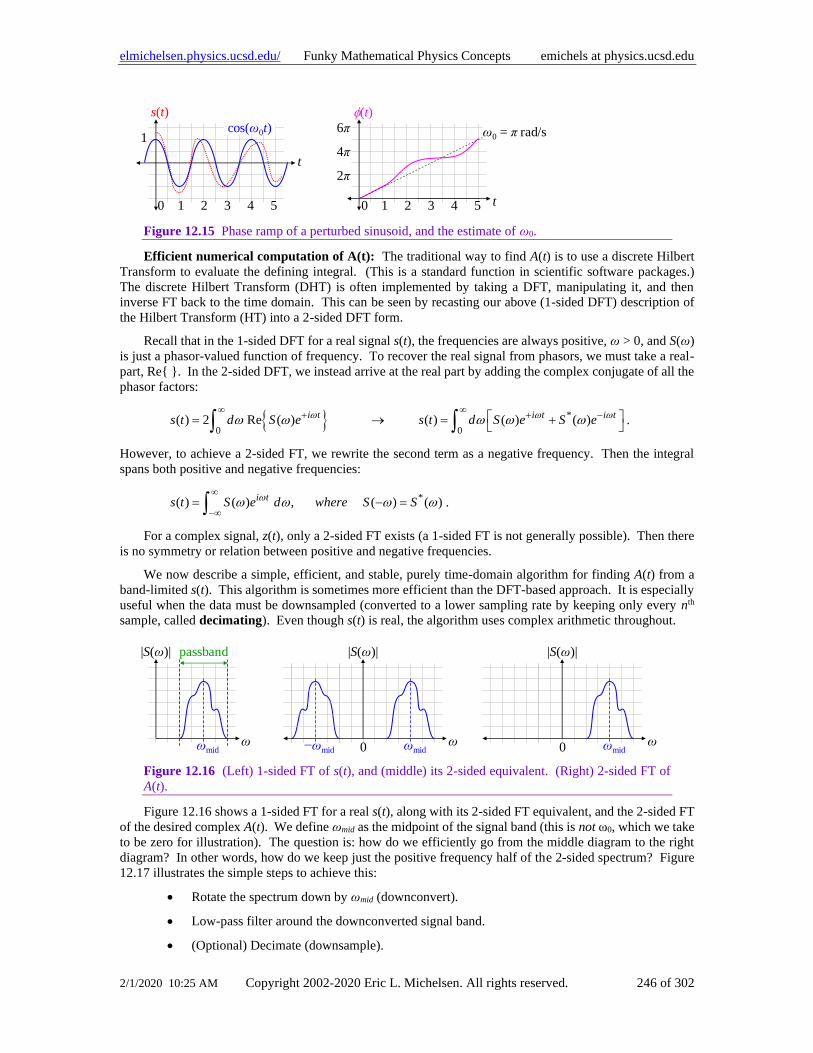
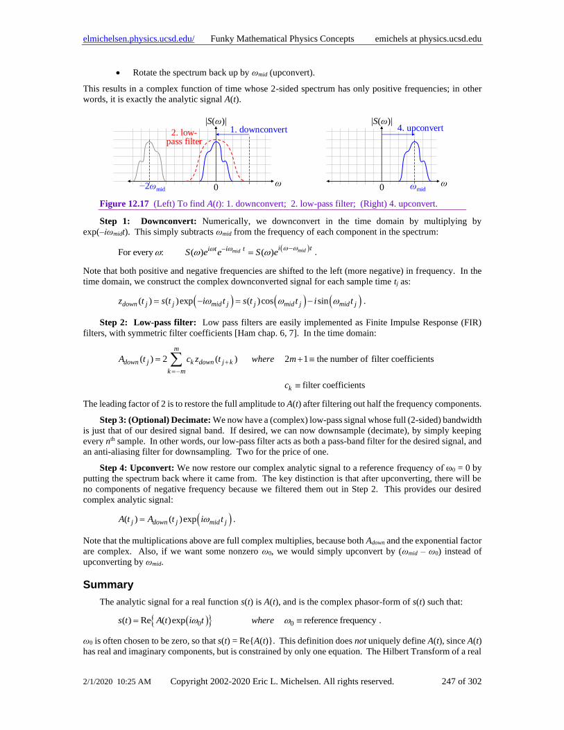
12 Fourier Transforms and Digital Signal Processing .........................................................................216 Model of Digitization and Sampling .............................................................................................217 Complex Sequences and Complex Fourier Transform ..................................................................217 Basis Functions and Orthogonality ...............................................................................................220 Real Sequences..............................................................................................................................221 Normalization and Parseval’s Theorem ........................................................................................222 Continuous and Discrete, Finite and Infinite .................................................................................224 White Noise and Correlation .........................................................................................................224 Why Oversampling Does Not Improve Signal-to-Noise Ratio .....................................................224 Filters TBS?? .................................................................................................................................225 What Happens to a Sine Wave Deferred? .....................................................................................225 Nonuniform Sampling and Arbitrary Basis Functions ..................................................................227 Don’t Pad Your Data, Even for FFTs............................................................................................229 Two Dimensional Fourier Transforms ..........................................................................................230 Note on Continuous Fourier Series and Uniform Convergence ....................................................230 Fourier Transforms, Periodograms, and Lomb-Scargle ................................................................231 The Discrete Fourier Transform vs. the Periodogram ...................................................................232 Practical Considerations ................................................................................................................233 The Lomb-Scargle Algorithm .......................................................................................................234 The Meaning Behind the Math ......................................................................................................235 Bandwidth Correction (aka Bandwidth Penalty) ...........................................................................239 Analytic Signals and Hilbert Transforms ......................................................................................242 Summary .......................................................................................................................................247
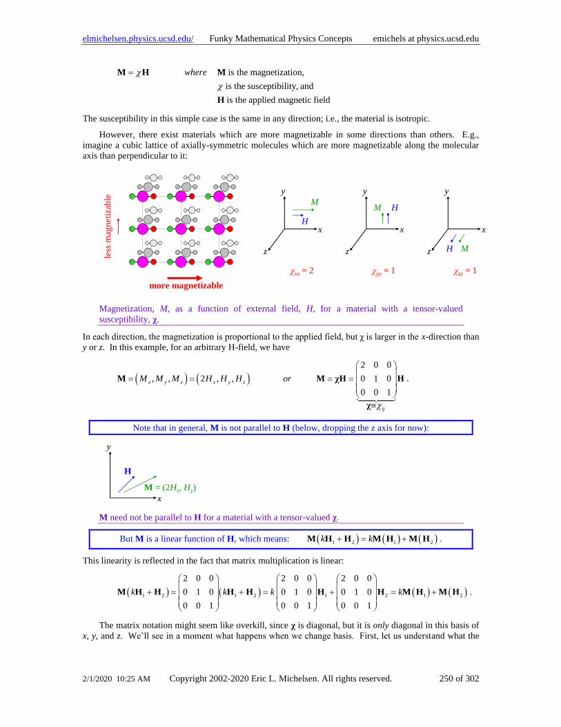
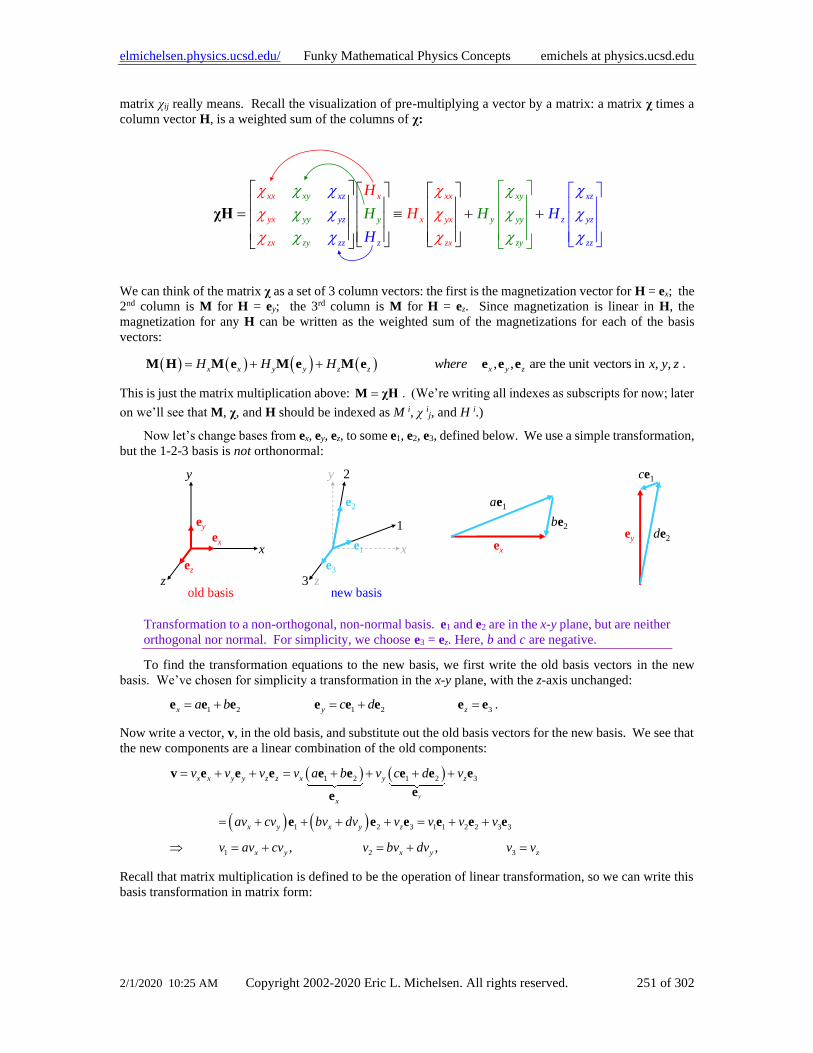
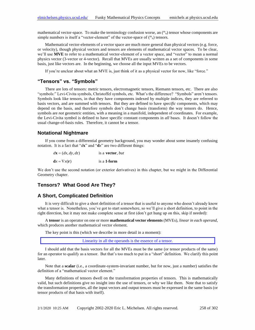
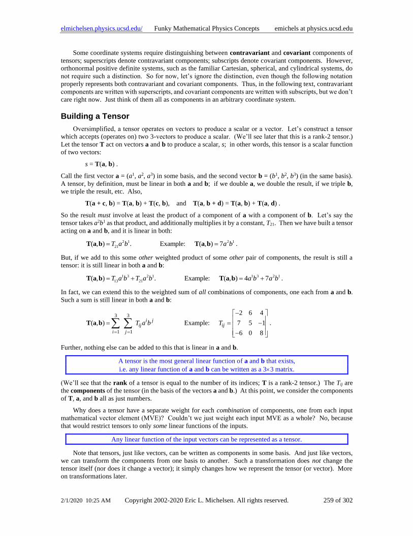
13 Tensors, Without the Tension ...........................................................................................................249 Approach .......................................................................................................................................249 Two Physical Examples ................................................................................................................249 Magnetic Susceptibility .................................................................................................................249 Mechanical Strain..........................................................................................................................253 When Is a Matrix Not a Tensor? ...................................................................................................255 Heading In the Right Direction .....................................................................................................255 Some Definitions and Review .......................................................................................................255 Vector Space Summary .................................................................................................................256 When Vectors Collide ...................................................................................................................257 “Tensors” vs. “Symbols”...............................................................................................................258 Notational Nightmare ....................................................................................................................258 Tensors? What Good Are They? ..................................................................................................258 A Short, Complicated Definition...................................................................................................258 Building a Tensor ..........................................................................................................................259 Tensors in Action ..........................................................................................................................260 Tensor Fields .................................................................................................................................261 Dot Products and Cross Products as Tensors ................................................................................261 The Danger of Matrices.................................................................................................................263 Reading Tensor Component Equations .........................................................................................263 Adding, Subtracting, Differentiating Tensors ...............................................................................264
Page 7
elmichelsen.physics.ucsd.edu/ Funky Mathematical Physics Concepts emichels at physics.ucsd.edu
2/1/2020 10:25 AM Copyright 2002-2020 Eric L. Michelsen. All rights reserved. 7 of 302
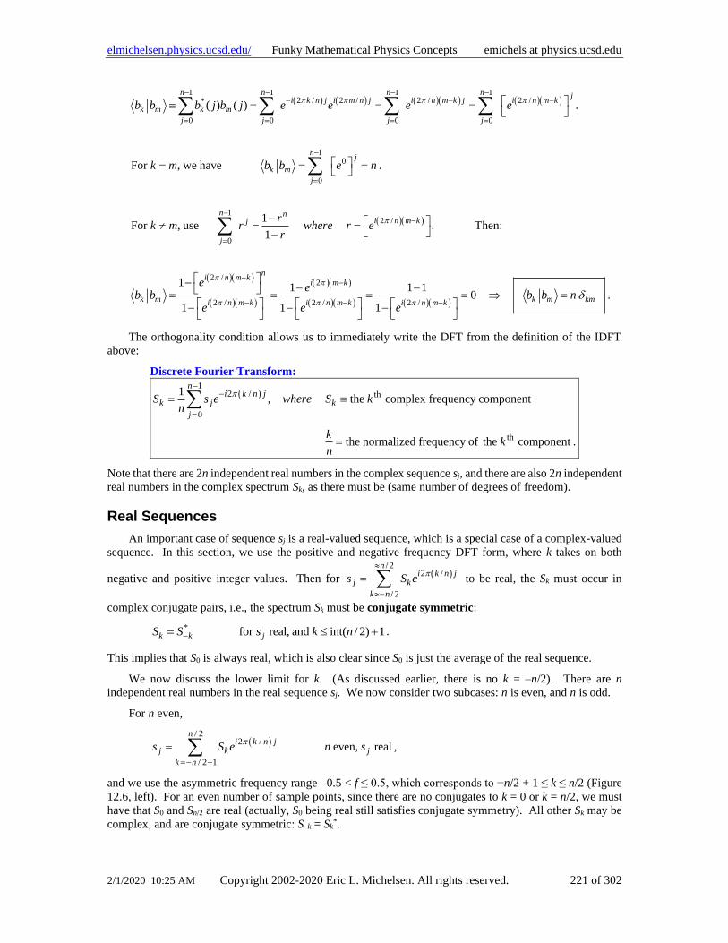
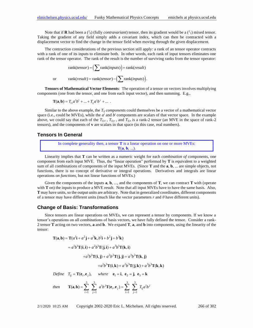
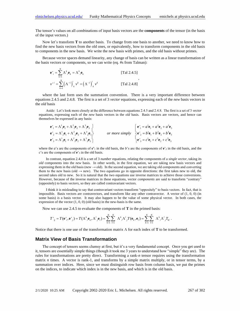
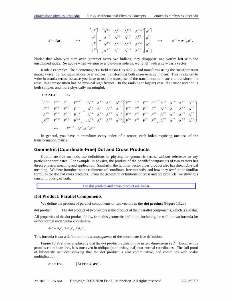
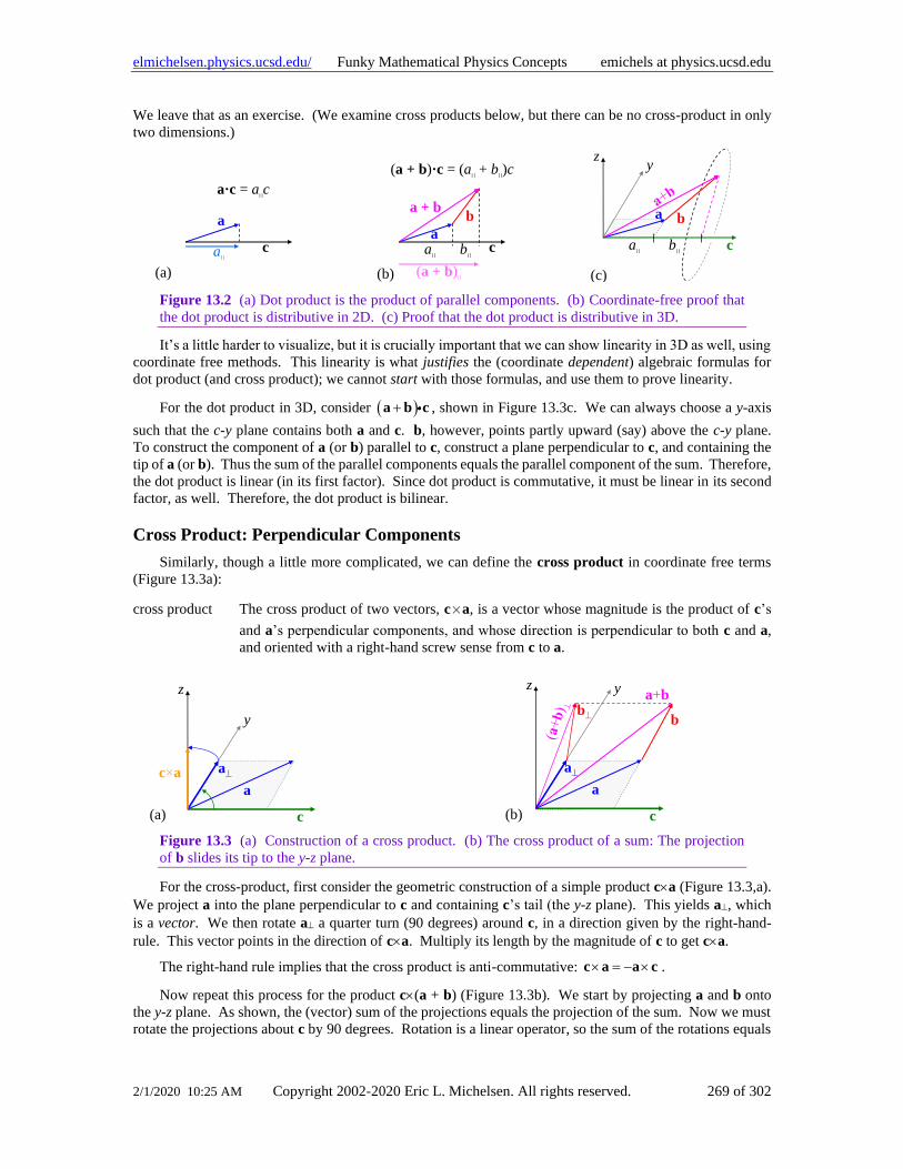
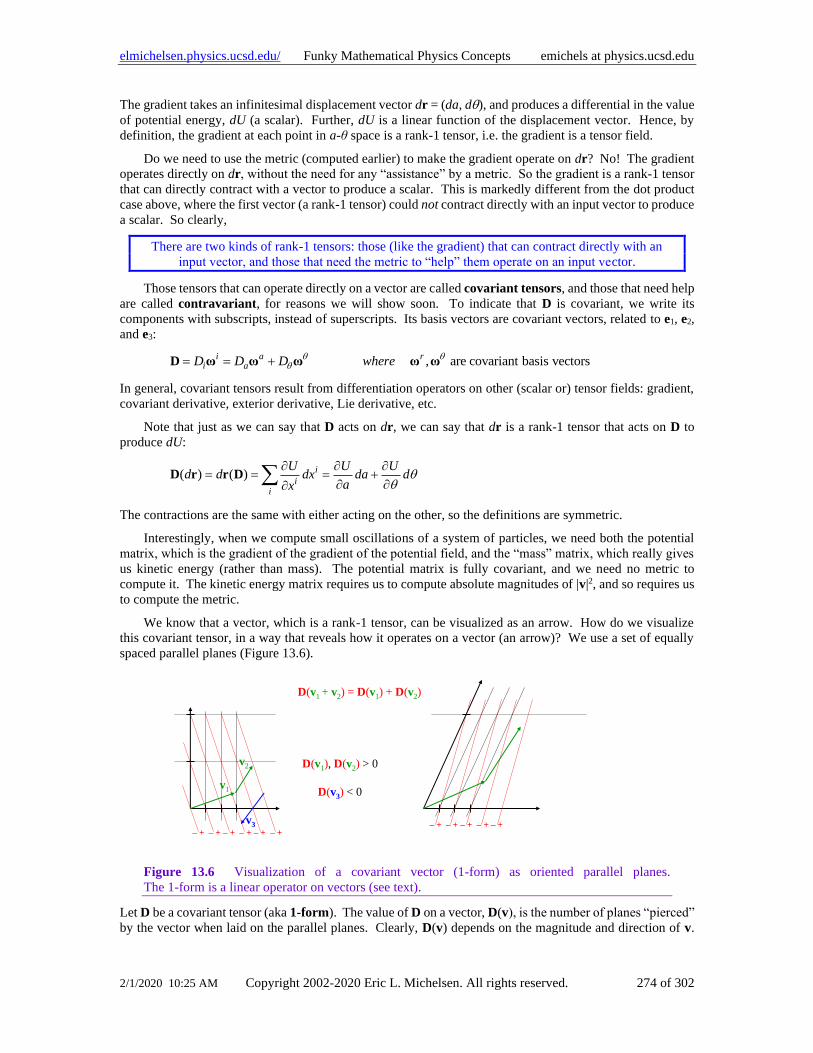
Higher Rank Tensors .....................................................................................................................264 Tensors In General ........................................................................................................................266 Change of Basis: Transformations ................................................................................................266 Matrix View of Basis Transformation ...........................................................................................267 Geometric (Coordinate-Free) Dot and Cross Products ..................................................................268 Non-Orthonormal Systems: Contravariance and Covariance........................................................270 Dot Products in Oblique Coordinates ............................................................................................270 Covariant Components of a Vector ...............................................................................................271 Example: Classical Mechanics with Oblique Generalized Coordinates ........................................272 What Goes Up Can Go Down: Duality of Contravariant and Covariant Vectors .........................275 The Real Summation Convention .................................................................................................276 Transformation of Covariant Indexes ............................................................................................276 Indefinite Metrics: Relativity ........................................................................................................277 Is a Transformation Matrix a Tensor? ...........................................................................................277 How About the Pauli Vector? .......................................................................................................278 Cartesian Tensors ..........................................................................................................................278 The Real Reason Why the Kronecker Delta Is Symmetric ...........................................................279 Tensor Appendices ........................................................................................................................279 Pythagorean Relation for 1-forms .................................................................................................279 Geometric Construction Of The Sum Of Two 1-Forms: ...............................................................281 “Fully Anti-symmetric” Symbols Expanded .................................................................................281 Metric? We Don’t Need No Stinking Metric! ..............................................................................282 References: ....................................................................................................................................284
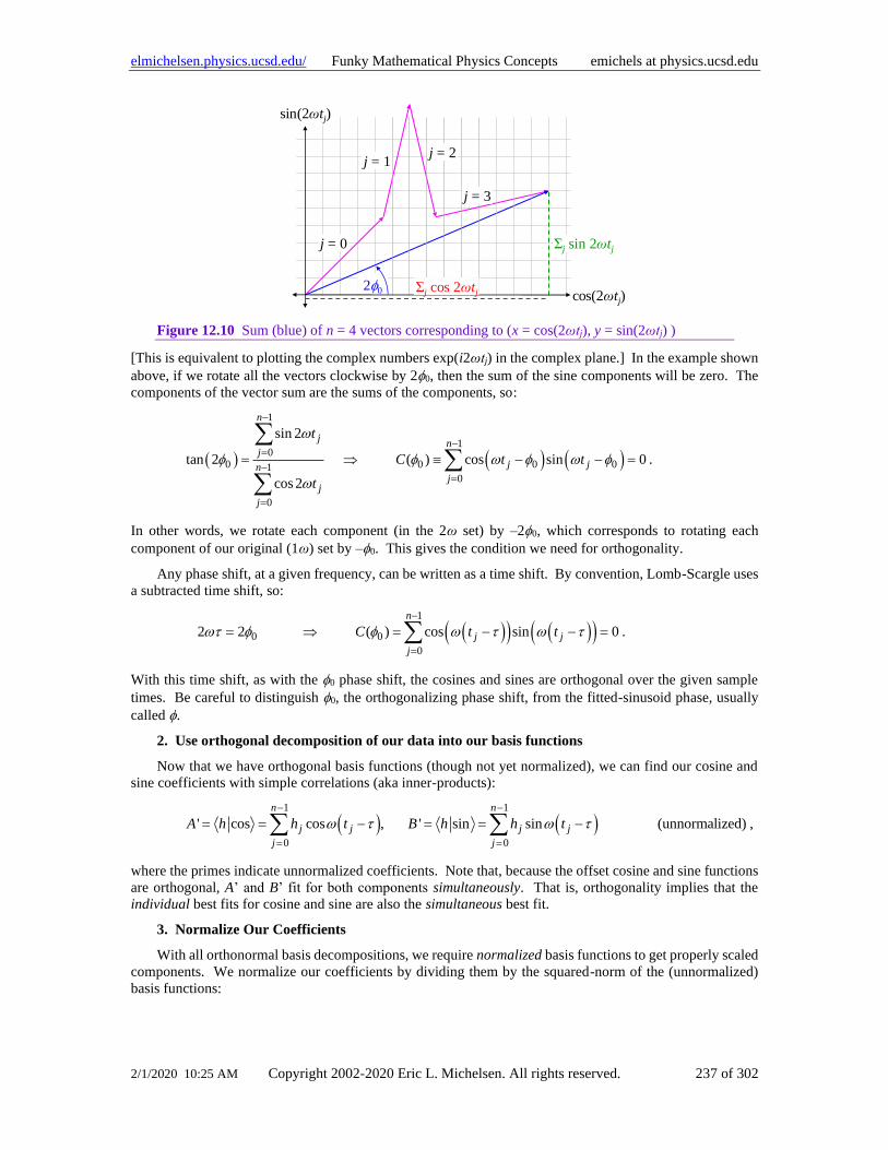
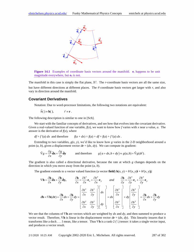
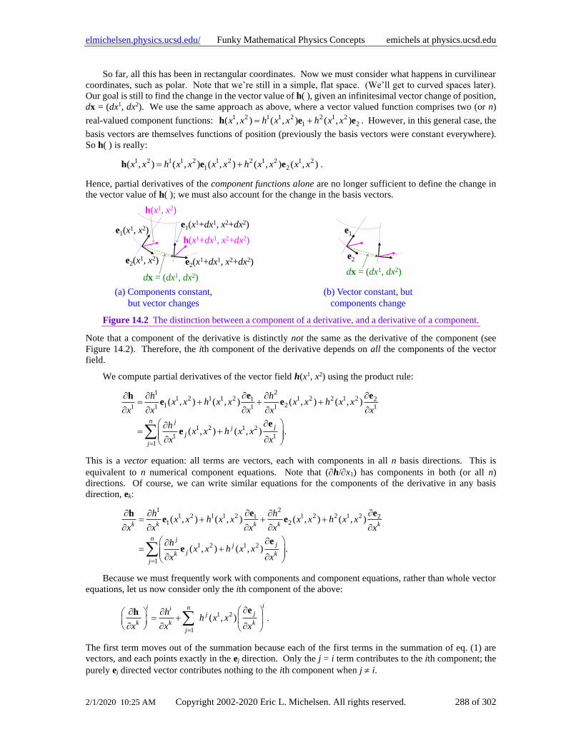
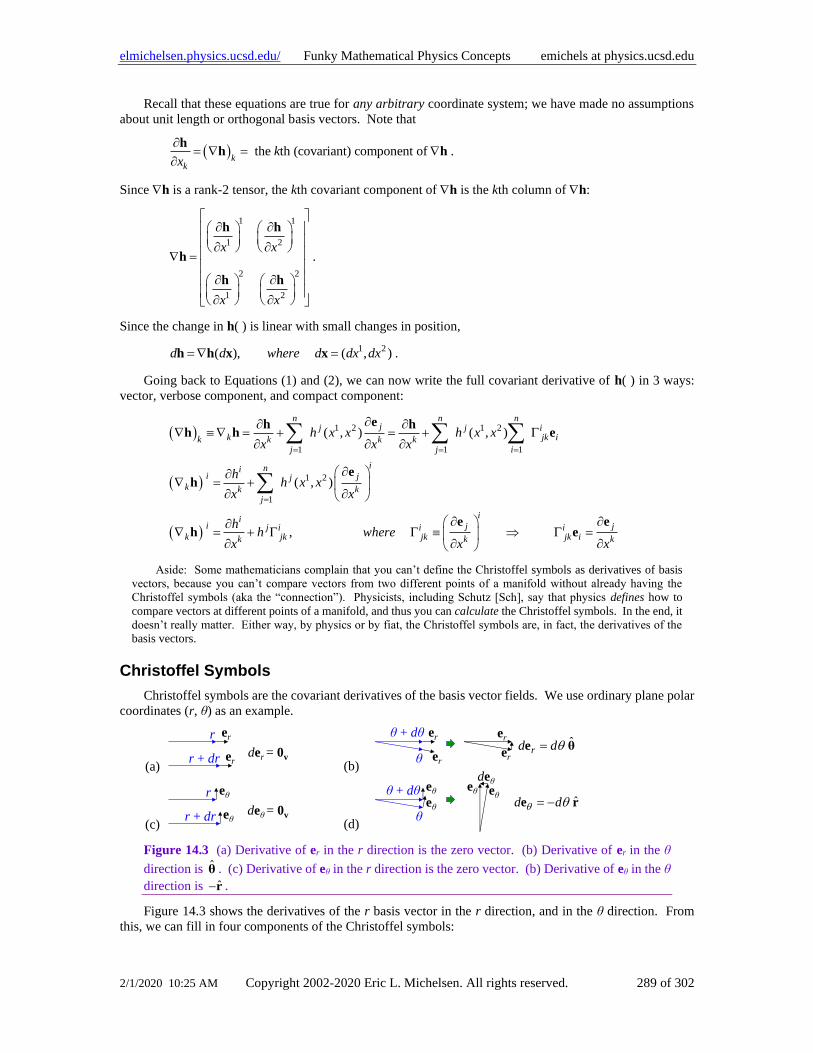
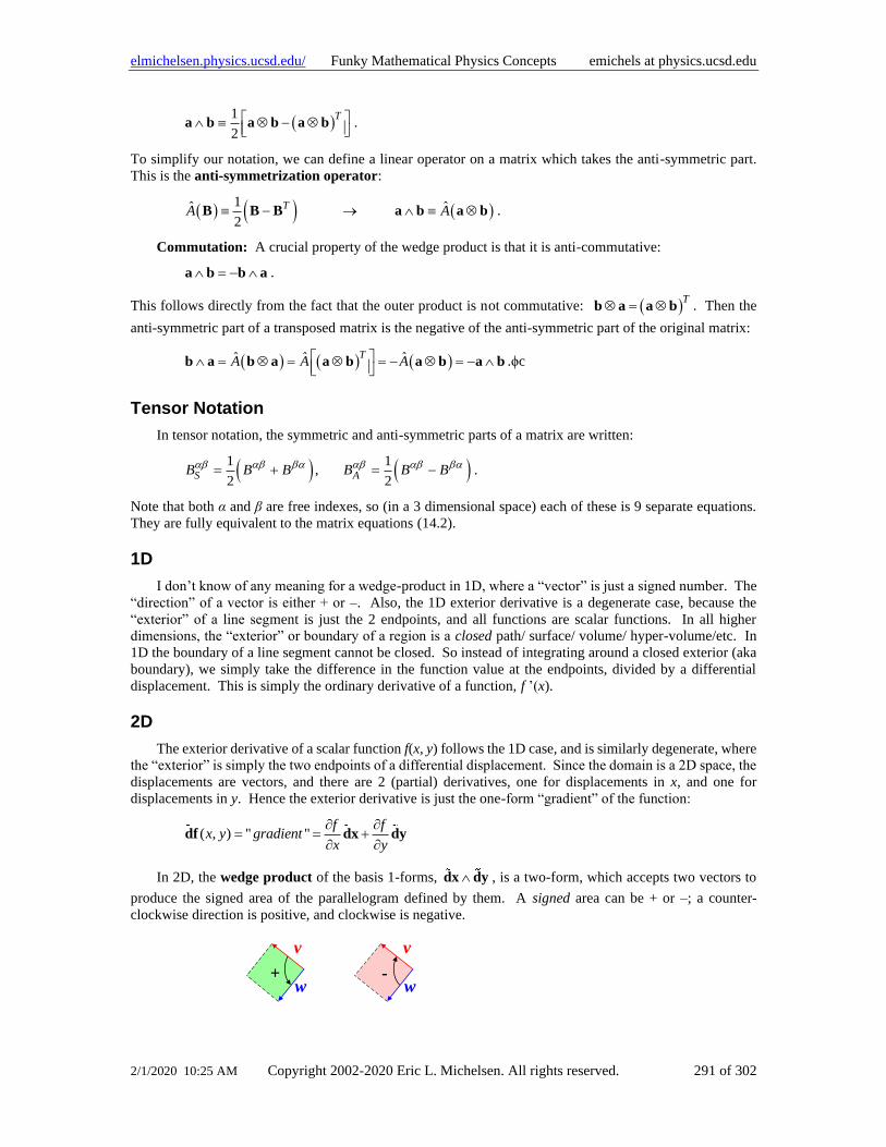
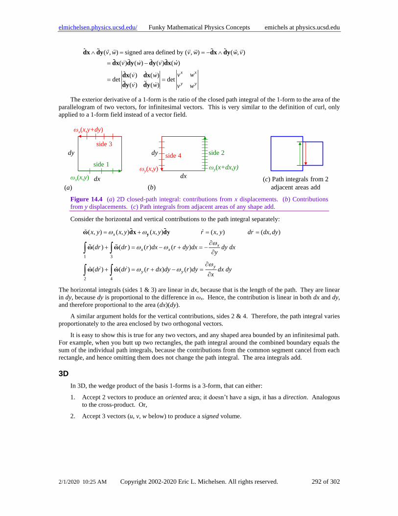
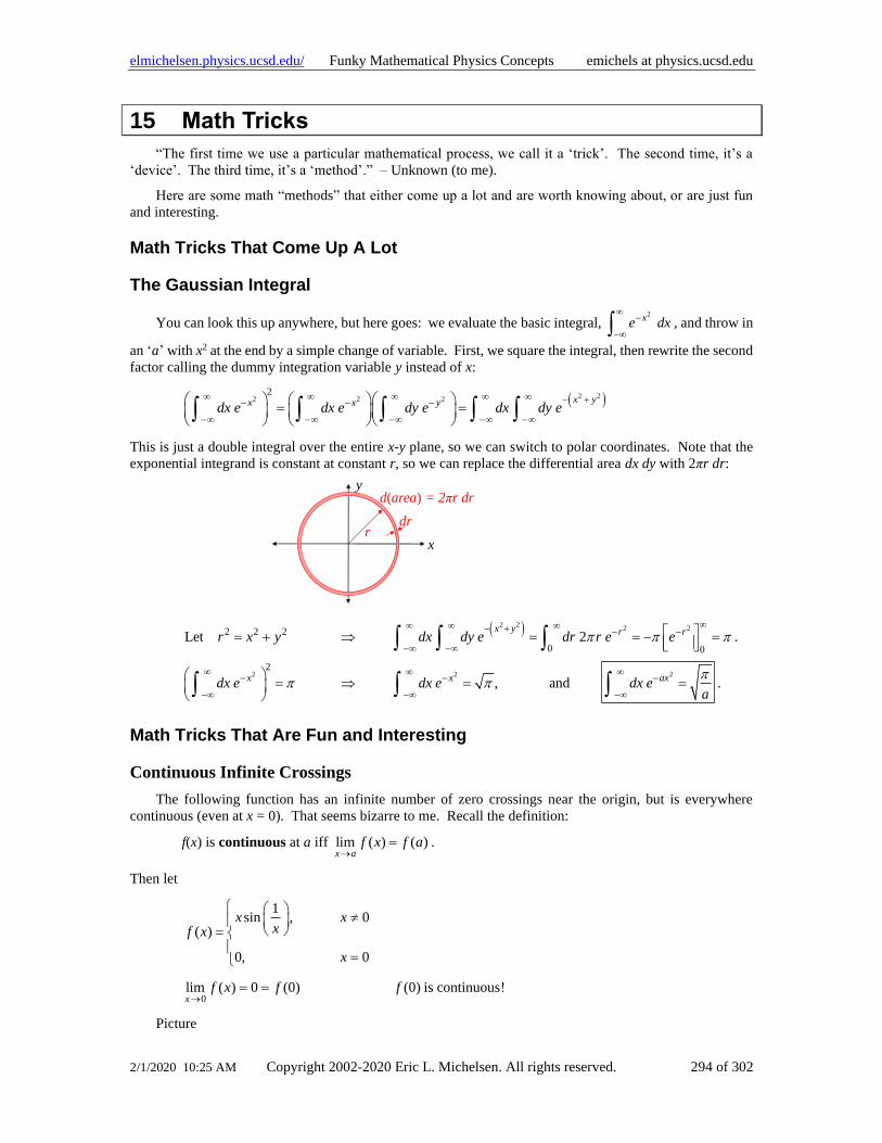
14 Differential Geometry ........................................................................................................................285 Manifolds ......................................................................................................................................285 Coordinate Bases ...........................................................................................................................285 Covariant Derivatives ....................................................................................................................287 Christoffel Symbols ......................................................................................................................289 Visualization of n-Forms ...............................................................................................................290 Review of Wedge Products and Exterior Derivative.....................................................................290 Wedge Products ............................................................................................................................290 Tensor Notation .............................................................................................................................291 1D ..................................................................................................................................................291 2D ..................................................................................................................................................291 3D ..................................................................................................................................................292
15 Math Tricks ........................................................................................................................................294 Math Tricks That Come Up A Lot ................................................................................................294 The Gaussian Integral ...................................................................................................................294 Math Tricks That Are Fun and Interesting ....................................................................................294 Phasors ..........................................................................................................................................295 Future Funky Mathematical Physics Topics .................................................................................295
16 Appendices ..........................................................................................................................................296 References .....................................................................................................................................296 Glossary ........................................................................................................................................296 Formulas........................................................................................................................................301 Index .............................................................................................................................................302
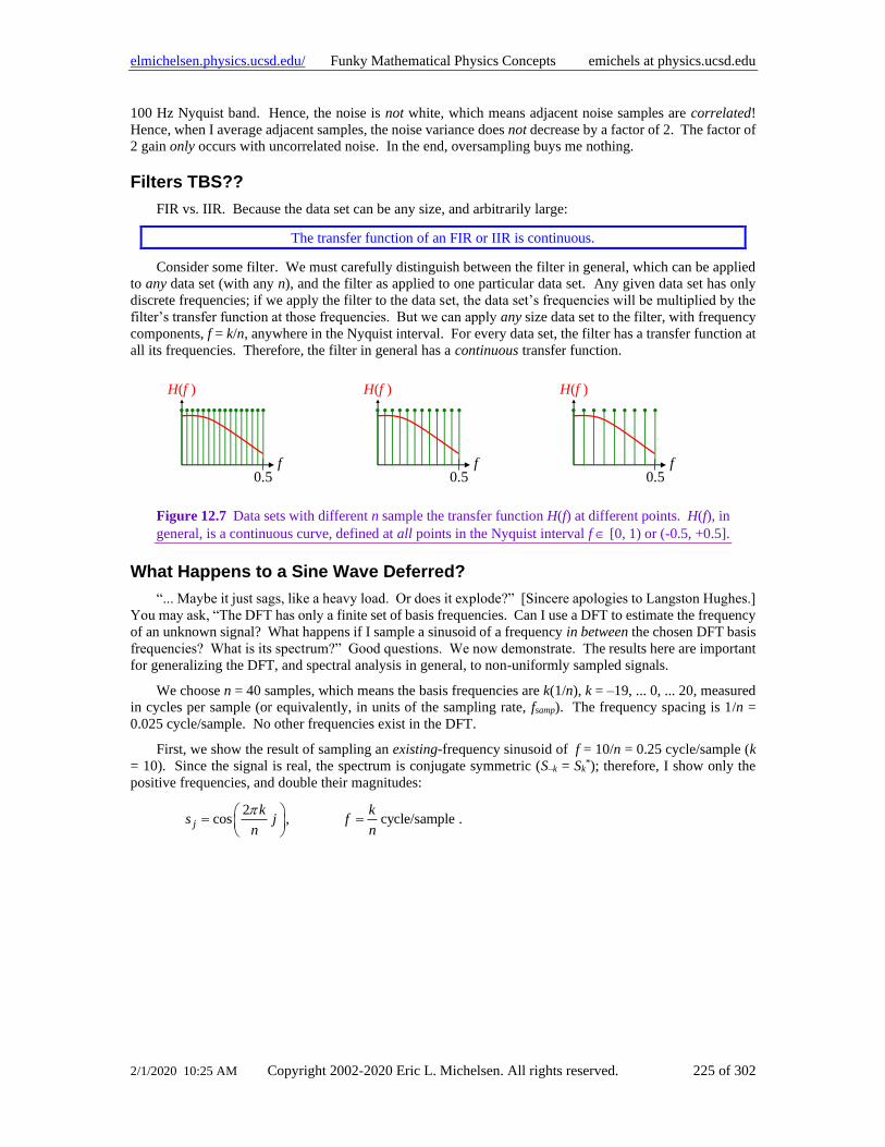
Page 8
elmichelsen.physics.ucsd.edu/ Funky Mathematical Physics Concepts emichels at physics.ucsd.edu
2/1/2020 10:25 AM Copyright 2002-2020 Eric L. Michelsen. All rights reserved. 8 of 302
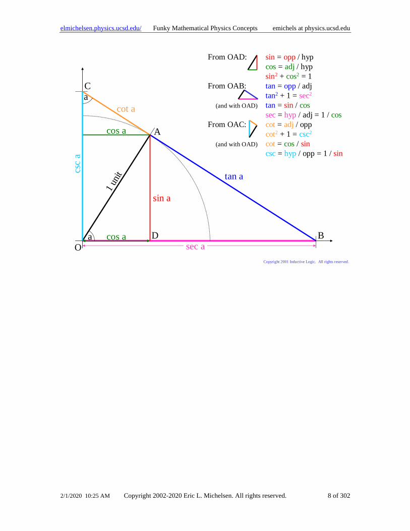
a cos a
sin a
1 un
it tan a
cot a
sec a
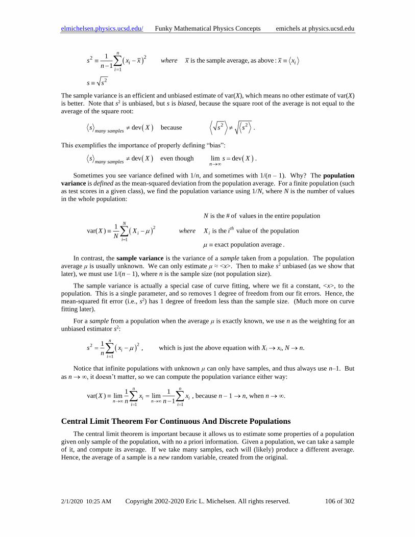
csc
a
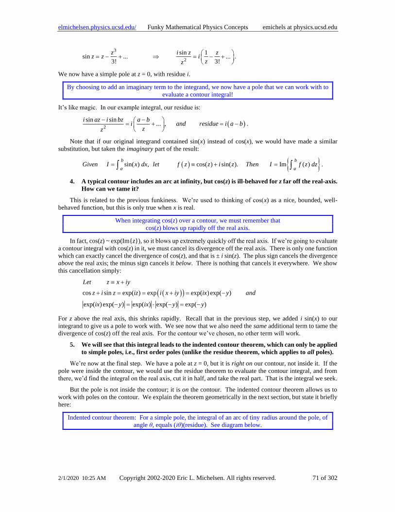
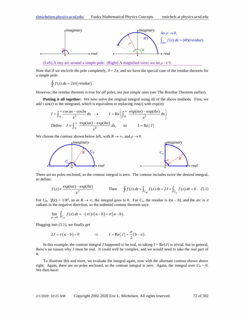
O
A
B
C
D
a
Copyright 2001 Inductive Logic. All rights reserved.
cos a
From OAD: sin = opp / hyp
cos = adj / hyp
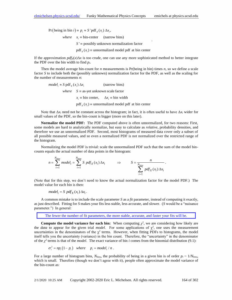
sin2 + cos2 = 1
From OAB: tan = opp / adj
tan2 + 1 = sec2
(and with OAD) tan = sin / cos
sec = hyp / adj = 1 / cos
From OAC: cot = adj / opp
cot2 + 1 = csc2
(and with OAD) cot = cos / sin
csc = hyp / opp = 1 / sin
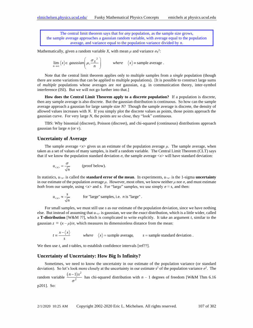
Page 9
elmichelsen.physics.ucsd.edu/ Funky Mathematical Physics Concepts emichels at physics.ucsd.edu
2/1/2020 10:25 AM Copyright 2002-2020 Eric L. Michelsen. All rights reserved. 9 of 302
1 Introduction
Mathematical Physics, or Physical Mathematics?
Is There Another Kind of Physics? Mathematical Physics is devoted to the natural emergence of
mathematics from our curiosity about the universe around us. All physics is mathematical, but Mathematical
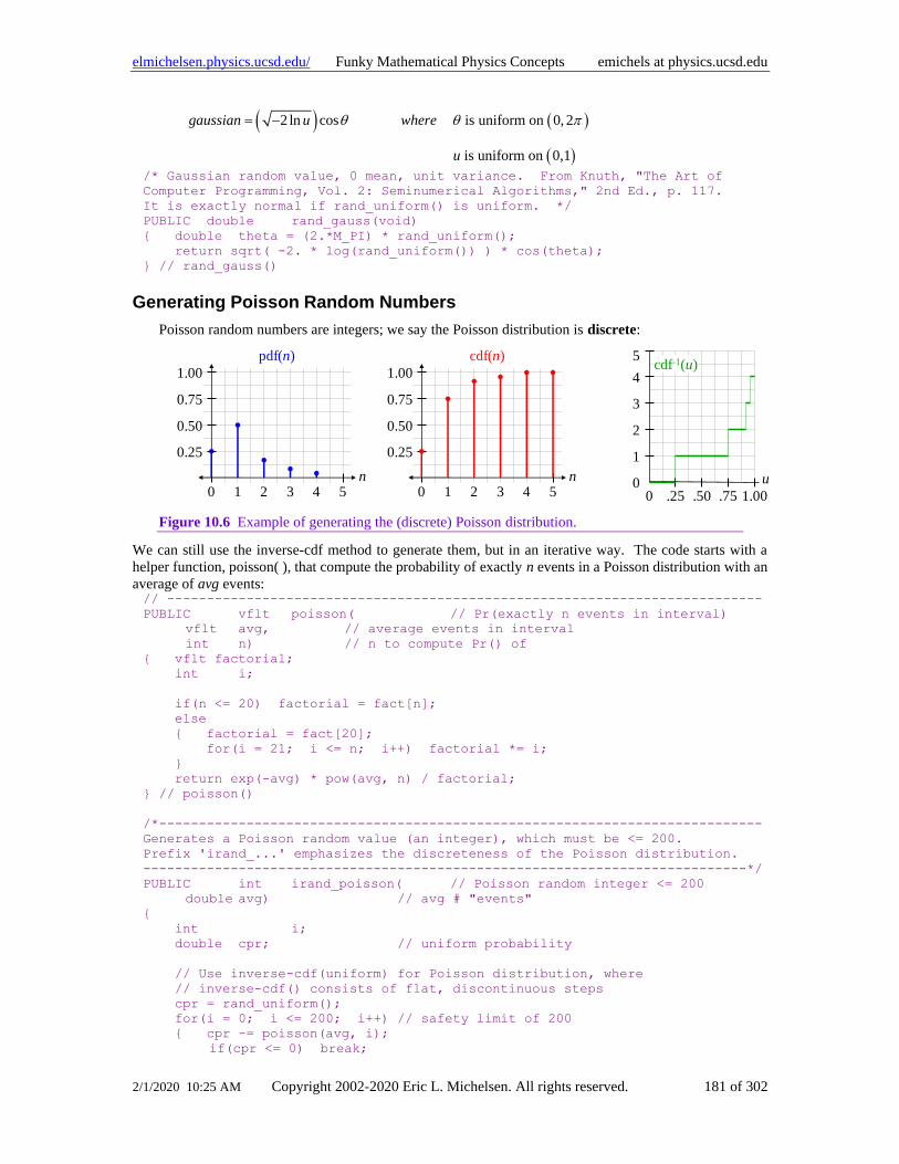
Physics illustrates that math is not abstract, or capricious, but an inescapable part of the natural world.
Despite its humble beginnings rooted in conceptual understanding and the practice of science, many find that
Mathematical Physics holds a beauty and fascination all its own.
As with all “Funky” notes, we emphasize the physical meaning of the underlying concepts. For example,
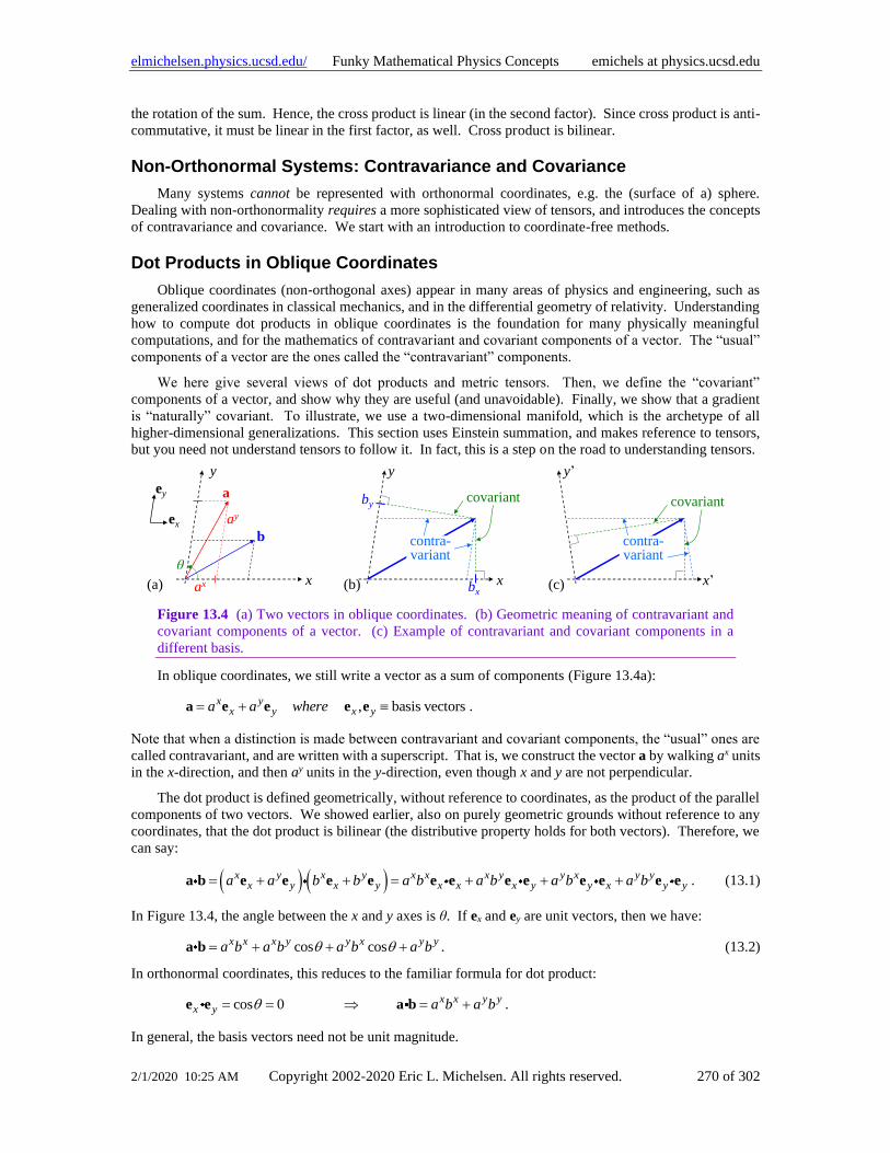
we stress a coordinate-free, geometric approach to vector operations.
Why Physicists and Mathematicians Argue
Physics goals and mathematics goals are antithetical. Physics seeks to ascribe meaning to mathematics
that describe the world, to “understand” it, physically. Mathematics seeks to strip the equations of all physical
meaning, and view them in purely abstract terms. These divergent goals set up a natural conflict between the
two camps. Each goal has its merits: the value of physics is (or should be) self-evident; the value of
mathematical abstraction, separate from any single application, is generality: the results can be used on a
wide range of applications.
Why Funky?
The purpose of the “Funky” series of documents is to help develop an accurate physical, conceptual,
geometric, and pictorial understanding of important physics topics. We focus on areas that don’t seem to be
covered well in most texts. The Funky series attempts to clarify those neglected concepts, and others that
seem likely to be challenging and unexpected (funky?). The Funky documents are intended for serious
students of physics; they are not “popularizations” or oversimplifications.
Physics includes math, and we’re not shy about it, but we also don’t hide behind it.
Without a conceptual understanding, math is gibberish.
This work is one of several aimed at graduate and advanced-undergraduate physics students. Go to our
web page (in the page header) for the latest versions of the Funky Series, and for contact information. We’re
looking for feedback, so please let us know what you think.
How to Use This Document
This work is not a text book.
There are plenty of those, and they cover most of the topics quite well. This work is meant to be used
with a standard text, to help emphasize those things that are most confusing for new students. When standard
presentations don’t make sense, come here.
You should read all of this introduction to familiarize yourself with the notation and contents. After that,
this work is meant to be read in the order that most suits you. Each section stands largely alone, though the
sections are ordered logically. Simpler material generally appears before more advanced topics. You may
read it from beginning to end, or skip around to whatever topic is most interesting. The “Shorts” chapter is
a diverse set of very short topics, meant for quick reading.
If you don’t understand something, read it again once, then keep reading.
Don’t get stuck on one thing. Often, the following discussion will clarify things.
The index is not yet developed, so go to the web page on the front cover, and text-search in this document.
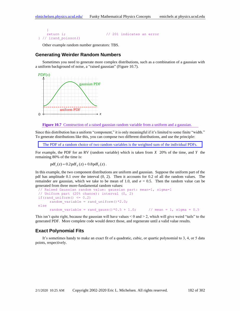
Page 10
elmichelsen.physics.ucsd.edu/ Funky Mathematical Physics Concepts emichels at physics.ucsd.edu
2/1/2020 10:25 AM Copyright 2002-2020 Eric L. Michelsen. All rights reserved. 10 of 302
Thank You
I owe a big thank you to many professors at both SDSU and UCSD, for their generosity even when I
wasn’t a real student: Dr. Herbert Shore, Dr. Peter Salamon, Dr. Arlette Baljon , Dr. Andrew Cooksy, Dr.
George Fuller, Dr. Tom O’Neil, Dr. Terry Hwa, and others.
Scope
What This Text Covers
This text covers some of the unusual or challenging concepts in graduate mathematical physics. It is
also very suitable for upper-division undergraduate level, as well. We expect that you are taking or have
taken such a course, and have a good text book. Funky Mathematical Physics Concepts supplements those
other sources.
What This Text Doesn’t Cover
This text is not a mathematical physics course in itself, nor a review of such a course. We do not cover
all basic mathematical concepts; only those that are very important, unusual, or especially challenging
(funky?).
What You Already Know
This text assumes you understand basic integral and differential calculus, and partial differential
equations. Further, it assumes you have a mathematical physics text for the bulk of your studies, and are
using Funky Mathematical Physics Concepts to supplement it.
Notation
Sometimes the variables are inadvertently not written in italics, but I hope the meanings are clear.
?? refers to places that need more work.
TBS To be supplied (one hopes) in the future.
Interesting points that you may skip are “asides,” shown in smaller font and narrowed margins. Notes to myself
may also be included as asides.
Common misconceptions are sometimes written in dark red dashed-line boxes.
Formulas: We write the integral over the entire domain as a subscript “∞”, for any number of
dimensions:
31-D: 3-D:dx d x
Evaluation between limits: we use the notation [function]ab to denote the evaluation of the function
between a and b, i.e.,
[f(x)]ab ≡ f(b) – f(a). For example, ∫ 01 3x2 dx = [x3]0
1 = 13 - 03 = 1.
We write the probability of an event as “Pr(event).”
Column vectors: Since it takes a lot of room to write column vectors, but it is often important to
distinguish between column and row vectors, I sometimes save vertical space by using the fact that a column
vector is the transpose of a row vector:
Page 11
elmichelsen.physics.ucsd.edu/ Funky Mathematical Physics Concepts emichels at physics.ucsd.edu
2/1/2020 10:25 AM Copyright 2002-2020 Eric L. Michelsen. All rights reserved. 11 of 302
( ), , ,T
a
ba b c d
c
d
=
Random variables: We use a capital letter, e.g. X, to represent the population from which instances of
a random variable, x (lower case), are observed. In a sense, X is a representation of the PDF of the random
variable, pdfX(x).
We denote that a random variable X comes from a population PDF as: X pdfX, e.g.: X χ2n. To denote
that X is a constant times a random variable from pdfY, we write: X k pdfY, e.g. X k χ2n.
For Greek letters, pronunciations, and use, see Quirky Quantum Concepts. Other math symbols:
Symbol Definition
for all
there exists
such that
iff if and only if
proportional to. E.g., a b means “a is proportional to b”
⊥ perpendicular to
therefore
of the order of (sometimes used imprecisely as “approximately equals”)
is defined as; identically equal to (i.e., equal in all cases)
implies
→ leads to
tensor product, aka outer product
direct sum
In mostly older texts, German type (font: Fraktur) is used to provide still more variable names:
Latin
German
Capital
German
Lowercase Notes
A A a Distinguish capital from U, V
B B b
C C c Distinguish capital from E, G
D D d Distinguish capital from O, Q
E E e Distinguish capital from C, G
F F f
G G g Distinguish capital from C, E
H H h
I I i Capital almost identical to J
J J j Capital almost identical to I
Page 12
elmichelsen.physics.ucsd.edu/ Funky Mathematical Physics Concepts emichels at physics.ucsd.edu
2/1/2020 10:25 AM Copyright 2002-2020 Eric L. Michelsen. All rights reserved. 12 of 302
K K k
L L l
M M m Distinguish capital from W
N N n
O O o Distinguish capital from D, Q
P P p
Q Q q Distinguish capital from D, O
R R r Distinguish lowercase from x
S S s Distinguish capital from C, G, E
T T t Distinguish capital from I
U U u Distinguish capital from A, V
V V v Distinguish capital from A, U
W W w Distinguish capital from M
X X x Distinguish lowercase from r
Y Y y
Z Z z
Page 13
elmichelsen.physics.ucsd.edu/ Funky Mathematical Physics Concepts emichels at physics.ucsd.edu
2/1/2020 10:25 AM Copyright 2002-2020 Eric L. Michelsen. All rights reserved. 13 of 302
2 Random Short Topics
I Always Lie
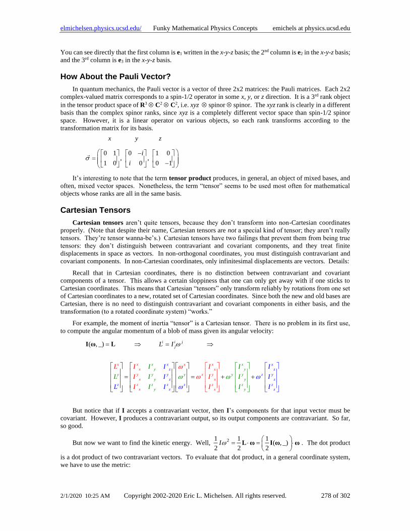
Logic, and logical deduction, are essential elements of all science. Too many of us acquire our logical
reasoning abilities only through osmosis, without any concrete foundation. Unfortunately, two of the most
commonly given examples of logical reasoning are both wrong. I found one in a book about Kurt Gödel (!),
the famous logician.
Fallacy #1: Consider the statement, “I always lie.” Wrong claim: this is a contradiction, and cannot be
either true or false. Right answer: this is simply false. The negation of “I always lie” is not “I always tell the
truth;” it is “I don’t always lie,” equivalent to “I at least sometimes tell the truth.” Since “I always lie” cannot
be true, it must be false, and it must be one of my (exceedingly rare) lies.
Fallacy #2: Consider the statement, “The barber shaves everyone who doesn’t shave himself. Who
shaves the barber?” Wrong answer: it’s a contradiction, and has no solution. Right answer: the barber shaves
himself. The original statement is about people who don’t shave themselves; it says nothing about people
who do shave themselves. If A then B; but if not A, then we know nothing about B. The barber does shave
everyone who does not shave himself, and he also shaves one person who does shave himself: himself. To
be a contradiction, the claim would need to be something like, “The barber shaves all and only those who
don’t shave themselves.”
Logic matters.
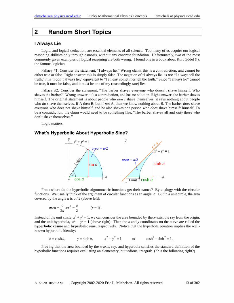
What’s Hyperbolic About Hyperbolic Sine?
x
sinh aarea = a/2
y
y = x
x2 – y2 = 1
cos a
sin a
x2 + y2 = 1
x
y
area = a/2
1 un
it
cosh a1 unit
a
From where do the hyperbolic trigonometric functions get their names? By analogy with the circular
functions. We usually think of the argument of circular functions as an angle, a. But in a unit circle, the area
covered by the angle a is a / 2 (above left):
2 ( 1)2 2
a aarea r r
= = = .
Instead of the unit circle, x2 + y2 = 1, we can consider the area bounded by the x-axis, the ray from the origin,
and the unit hyperbola, x2 – y2 = 1 (above right). Then the x and y coordinates on the curve are called the
hyperbolic cosine and hyperbolic sine, respectively. Notice that the hyperbola equation implies the well-
known hyperbolic identity:
2 2 2 2cosh , sinh , 1 cosh sinh 1x a y a x y= = − = − = .
Proving that the area bounded by the x-axis, ray, and hyperbola satisfies the standard definition of the
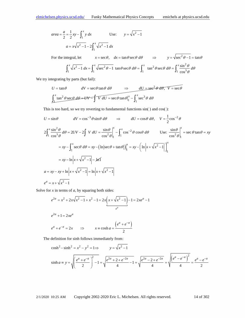
hyperbolic functions requires evaluating an elementary, but tedious, integral: (?? is the following right?)
Page 14
elmichelsen.physics.ucsd.edu/ Funky Mathematical Physics Concepts emichels at physics.ucsd.edu
2/1/2020 10:25 AM Copyright 2002-2020 Eric L. Michelsen. All rights reserved. 14 of 302
2
1
2 2
1
2
22 2 2
31 1 1 1
1Use: 1
2 2
1 2 1
For the integral, let sec , tan sec sec 1 tan
sin1 sec 1 tan sec tan sec
cos
x
x
x x x x
aarea xy y dx y x
a x x x dx
x dx d y
x dx d d d
= = − = −
= − − −
= = = − =
− = − = =
We try integrating by parts (but fail):
2
2 3
11 1
tan sec tan sec , sec
tan sec sec tan secx xx
U dV d dU d V
d UV V dU d
= = = =
= − = −
This is too hard, so we try reverting to fundamental functions sin( ) and cos( ):
( )
3 2
22
3 2 21 11 1
2
11 1
2
1sin cos sin cos , cos
2
sin sin sin2 2 2 cos cos Use: sec tan
cos cos cos
sec ln sec tan ln 1
ln 1 ln1
x xx x
xx x
U dV d dU d V
d UV V dU d xy
xy d xy xy x x
xy x x
− −
−
= = = =
= − = − = =
= − = − + = − + −
= − + − −
2 2
2
ln 1 ln 1
1a
a xy xy x x x x
e x x
= − + + − = + −
= + −
Solve for x in terms of a, by squaring both sides:
( )
( )
2 2 2 2 2
2
2 1 1 2 1 1 2 1
1 2
2 cosh2
a
a a
e
a a
a a
a a
e x x x x x x x xe
e xe
e ee e x x a
−
−
= + − + − = + − − = −
+ =
++ = =
The definition for sinh follows immediately from:
( )
2 2 2 2 2
22
2 2 2 2
cosh sinh 1 1
2 2sinh 1 1
2 4 4 4 2
a aa a a a a a a a
x y y x
e ee e e e e e e ea y
−− − − −
− = − = = −
− + + + − + − = − = − = = =
Page 15
elmichelsen.physics.ucsd.edu/ Funky Mathematical Physics Concepts emichels at physics.ucsd.edu
2/1/2020 10:25 AM Copyright 2002-2020 Eric L. Michelsen. All rights reserved. 15 of 302
Basic Calculus You May Not Know
Amazingly, many calculus courses never provide a precise definition of a “limit,” despite the fact that
both of the fundamental concepts of calculus, derivatives and integrals, are defined as limits! So here we go:
Basic calculus relies on 4 major concepts:
1. Functions
2. Limits
3. Derivatives
4. Integrals
1. Functions: Briefly, (in real analysis) a function takes one or more real values as inputs, and produces
one or more real values as outputs. The inputs to a function are called the arguments. The simplest case is
a real-valued function of a real-valued argument e.g., f(x) = sin x. Mathematicians would write (f : R1 →
R1), read “f is a map (or function) from the real numbers to the real numbers.” A function which produces
more than one output may be considered a vector-valued function.
2. Limits: Definition of “limit” (for a real-valued function of a single argument, f : R1 → R1):
L is the limit of f(x) as x approaches a, iff for every ε > 0, there exists a δ (> 0) such that |f(x) – L| < ε whenever
0 < |x – a| < δ. In symbols:
lim ( ) iff 0, such that ( ) whenever 0x a
L f x f x L x a →
= − − .
This says that the value of the function at a doesn’t matter; in fact, most often the function is not defined at
a. However, the behavior of the function near a is important. If you can make the function arbitrarily close
to some number, L, by restricting the function’s argument to a small neighborhood around a, then L is the
limit of f as x approaches a.
Surprisingly, this definition also applies to complex functions of complex variables, where the absolute
value is the usual complex magnitude.
Example: Show that 2
1
2 2lim 4
1x
x
x→
−=
−.
Solution: We prove the existence of δ given any ε by computing the necessary δ from ε. Note that for 22 2
1, 2( 1)1
xx x
x
− = +
−. The definition of a limit requires that
22 24 whenever 0 1
1
xx
x
−− −
−.
We solve for x in terms of ε, which will then define δ in terms of ε. Since we don’t care what the function is
at x = 1, we can use the simplified form, 2(x + 1). When x = 1, this is 4, so we suspect the limit = 4. Proof:
2( 1) 4 2 ( 1) 2 1 1 12 2 2
x x x or x
+ − + − − − + .
So by setting δ = ε/2, we construct the required δ for any given ε. Hence, for every ε, there exists a δ satisfying
the definition of a limit.
3. Derivatives: Only now that we have defined a limit, can we define a derivative:
0
( ) ( )'( ) lim
x
f x x f xf x
x →
+ −
.
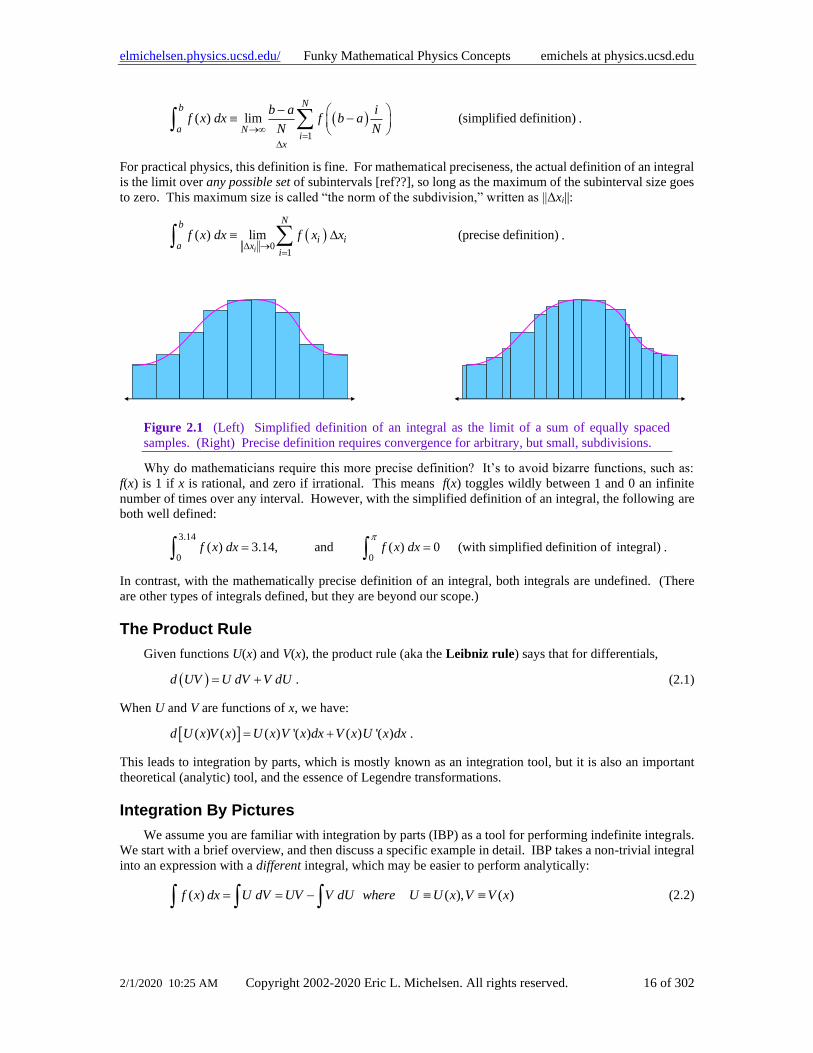
4. Integrals: A simplified definition of an integral is an infinite sum of areas under a function divided
into equal subintervals (Figure 2.1, left):
Page 16
elmichelsen.physics.ucsd.edu/ Funky Mathematical Physics Concepts emichels at physics.ucsd.edu
2/1/2020 10:25 AM Copyright 2002-2020 Eric L. Michelsen. All rights reserved. 16 of 302
( )1
( ) lim (simplified definition)
Nb
a Ni
x
b a if x dx f b a
N N→=
− −
.
For practical physics, this definition is fine. For mathematical preciseness, the actual definition of an integral
is the limit over any possible set of subintervals [ref??], so long as the maximum of the subinterval size goes
to zero. This maximum size is called “the norm of the subdivision,” written as ||Δxi||:
( )0
1
( ) lim (precise definition)i
Nb
i ia x
i
f x dx f x x →
=
.
Figure 2.1 (Left) Simplified definition of an integral as the limit of a sum of equally spaced
samples. (Right) Precise definition requires convergence for arbitrary, but small, subdivisions.
Why do mathematicians require this more precise definition? It’s to avoid bizarre functions, such as:
f(x) is 1 if x is rational, and zero if irrational. This means f(x) toggles wildly between 1 and 0 an infinite
number of times over any interval. However, with the simplified definition of an integral, the following are
both well defined:
3.14
0 0( ) 3.14, and ( ) 0 (with simplified definition of integral)f x dx f x dx
= = .
In contrast, with the mathematically precise definition of an integral, both integrals are undefined. (There
are other types of integrals defined, but they are beyond our scope.)
The Product Rule
Given functions U(x) and V(x), the product rule (aka the Leibniz rule) says that for differentials,
( )d UV U dV V dU= + . (2.1)
When U and V are functions of x, we have:
( ) ( ) ( ) '( ) ( ) '( )d U x V x U x V x dx V x U x dx= + .
This leads to integration by parts, which is mostly known as an integration tool, but it is also an important
theoretical (analytic) tool, and the essence of Legendre transformations.
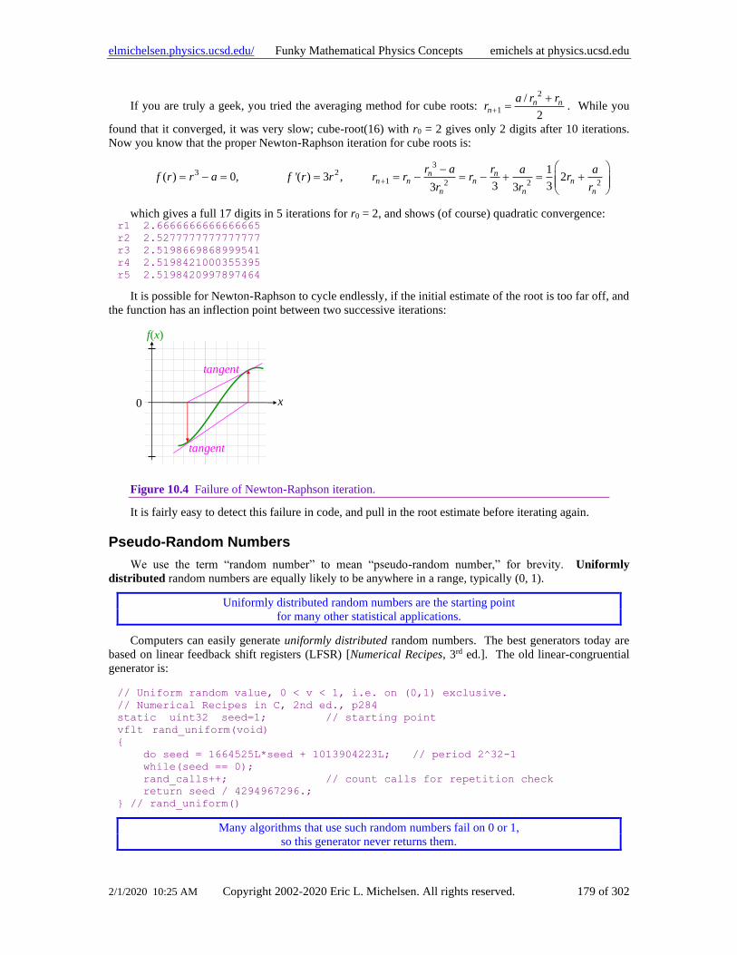
Integration By Pictures
We assume you are familiar with integration by parts (IBP) as a tool for performing indefinite integrals.
We start with a brief overview, and then discuss a specific example in detail. IBP takes a non-trivial integral
into an expression with a different integral, which may be easier to perform analytically:
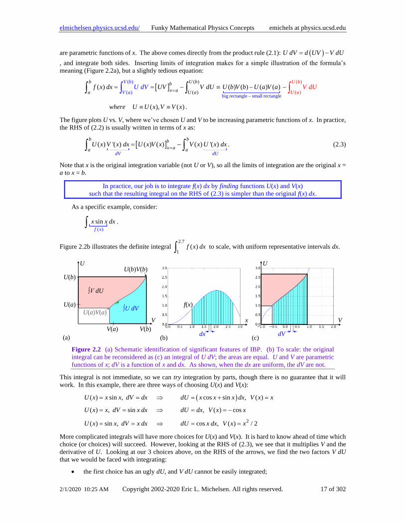
( ) ( ), ( )f x dx U dV UV V dU where U U x V V x = = − (2.2)
Page 17
elmichelsen.physics.ucsd.edu/ Funky Mathematical Physics Concepts emichels at physics.ucsd.edu
2/1/2020 10:25 AM Copyright 2002-2020 Eric L. Michelsen. All rights reserved. 17 of 302
are parametric functions of x. The above comes directly from the product rule (2.1): ( )U dV d UV V dU= −
, and integrate both sides. Inserting limits of integration makes for a simple illustration of the formula’s
meaning (Figure 2.2a), but a slightly tedious equation:
( )
( )big rectangle sma
)
ll rect
( ( )
angle( )( )
( ) ( ) ( ) ( ) ( )
( ), ( ) .
bV b U b
U axV a
b U b
aa U af x dx UV V dU U b V b U a V a
where U U x V V x
V dU V Ud
−
= = = − − −
The figure plots U vs. V, where we’ve chosen U and V to be increasing parametric functions of x. In practice,
the RHS of (2.2) is usually written in terms of x as:
( ) '( ) ( ) ( ) ( ) '( ) .b
dV d
b
aU
b
x a aU x V x dx U x V x V x U x dx
== − (2.3)
Note that x is the original integration variable (not U or V), so all the limits of integration are the original x =
a to x = b.
In practice, our job is to integrate f(x) dx by finding functions U(x) and V(x)
such that the resulting integral on the RHS of (2.3) is simpler than the original f(x) dx.
As a specific example, consider:
( )
sinf x
x x dx .
Figure 2.2b illustrates the definite integral 2.7
1( )f x dx to scale, with uniform representative intervals dx.
U
(a) (b) (c)
f(x)
Vx
dx dV
V
U
V(a) V(b)
U(a)
U(b)
U(b)V(b)
∫U dVU(a)V(a)
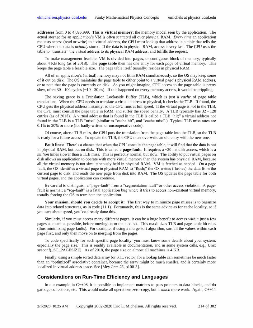
∫V dU
Figure 2.2 (a) Schematic identification of significant features of IBP. (b) To scale: the original
integral can be reconsidered as (c) an integral of U dV; the areas are equal. U and V are parametric
functions of x; dV is a function of x and dx. As shown, when the dx are uniform, the dV are not.
This integral is not immediate, so we can try integration by parts, though there is no guarantee that it will
work. In this example, there are three ways of choosing U(x) and V(x):
( )
2
( ) sin , cos sin , ( )
( ) , sin , ( ) cos
( ) sin , cos , ( ) / 2
U x x x dV dx dU x x x dx V x x
U x x dV x dx dU dx V x x
U x x dV x dx dU x dx V x x
= = = + =
= = = = −
= = = =
More complicated integrals will have more choices for U(x) and V(x). It is hard to know ahead of time which
choice (or choices) will succeed. However, looking at the RHS of (2.3), we see that it multiplies V and the
derivative of U. Looking at our 3 choices above, on the RHS of the arrows, we find the two factors V dU
that we would be faced with integrating:
• the first choice has an ugly dU, and V dU cannot be easily integrated;
Page 18
elmichelsen.physics.ucsd.edu/ Funky Mathematical Physics Concepts emichels at physics.ucsd.edu
2/1/2020 10:25 AM Copyright 2002-2020 Eric L. Michelsen. All rights reserved. 18 of 302
• the second choice has dU = dx, which literally could not be simpler, and V dU integrates easily;
• the last choice has dU = cos x dx, which isn’t bad, but V dU cannot be easily integrated.
Thus our best guess is the second choice (often, the simplest dU is a good choice). Figure 2.2c illustrates
U dV to scale; U and V are parametric functions of x; dV is a function of x and dx. Then:
sin cos cos cos sinUV V dU
x x dx x x x dx x x x = − − − = − + .
We check by differentiating the RHS above, which yields the original integrand.
Note that when the dx in Figure 2.2b are uniform, the dV in Figure 2.2c are not. However, all the dV go
to zero when the dx do, so the integral of U dV is still valid.
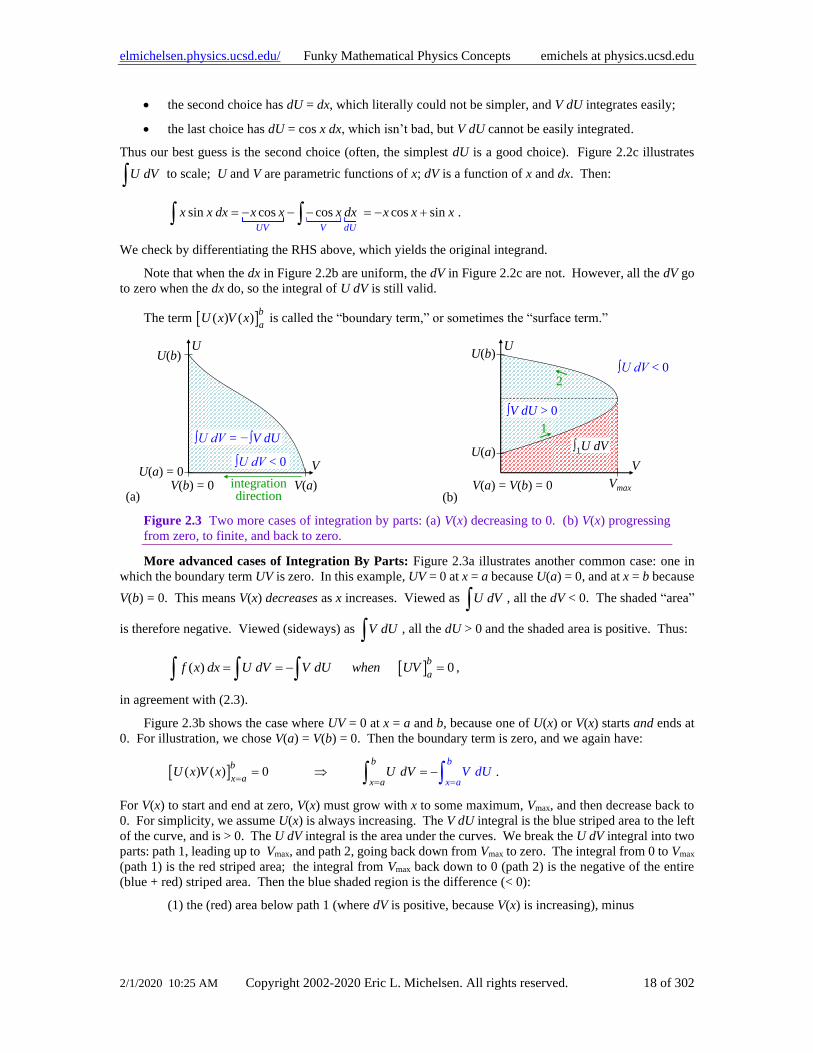
The term ( ) ( )b
aU x V x is called the “boundary term,” or sometimes the “surface term.”
U
U(a) = 0
U(b)
V(a)
∫U dV = −∫V dU
integrationdirection
V(b) = 0
VU(a)
U(b)
VmaxV(a) = V(b) = 0
∫V dU > 0
∫1U dV
1
2
U
V
(a) (b)
∫U dV < 0
∫U dV < 0
Figure 2.3 Two more cases of integration by parts: (a) V(x) decreasing to 0. (b) V(x) progressing
from zero, to finite, and back to zero.
More advanced cases of Integration By Parts: Figure 2.3a illustrates another common case: one in
which the boundary term UV is zero. In this example, UV = 0 at x = a because U(a) = 0, and at x = b because
V(b) = 0. This means V(x) decreases as x increases. Viewed as U dV , all the dV < 0. The shaded “area”
is therefore negative. Viewed (sideways) as V dU , all the dU > 0 and the shaded area is positive. Thus:
( ) 0b
af x dx U dV V dU when UV = = − = ,
in agreement with (2.3).
Figure 2.3b shows the case where UV = 0 at x = a and b, because one of U(x) or V(x) starts and ends at
0. For illustration, we chose V(a) = V(b) = 0. Then the boundary term is zero, and we again have:
( ) ( ) 0bb
x a x
b
x aaU x V x U d V dV U
= = == = − .
For V(x) to start and end at zero, V(x) must grow with x to some maximum, Vmax, and then decrease back to
0. For simplicity, we assume U(x) is always increasing. The V dU integral is the blue striped area to the left
of the curve, and is > 0. The U dV integral is the area under the curves. We break the U dV integral into two
parts: path 1, leading up to Vmax, and path 2, going back down from Vmax to zero. The integral from 0 to Vmax
(path 1) is the red striped area; the integral from Vmax back down to 0 (path 2) is the negative of the entire
(blue + red) striped area. Then the blue shaded region is the difference (< 0):
(1) the (red) area below path 1 (where dV is positive, because V(x) is increasing), minus
Page 19
elmichelsen.physics.ucsd.edu/ Funky Mathematical Physics Concepts emichels at physics.ucsd.edu
2/1/2020 10:25 AM Copyright 2002-2020 Eric L. Michelsen. All rights reserved. 19 of 302
(2) the (blue + red) area below path 2, where dV is negative because V(x) is decreasing. Thus
0U dV :
max max max
max
0
0
1 2
0 0
1 1 22
.
V
V V V
path path pathp
V V
V V
p p
b
x
t
a
a h athath
U dV U dVU
V dU
ddV U d U VV= ==
+
=
=
= + = −
= −
Page 20
elmichelsen.physics.ucsd.edu/ Funky Mathematical Physics Concepts emichels at physics.ucsd.edu
2/1/2020 10:25 AM Copyright 2002-2020 Eric L. Michelsen. All rights reserved. 20 of 302
Theoretical Importance of IBP
Besides being an integration tool, an important theoretical consequence of IBP is that the variable of
integration is changed, from dV to dU. Many times, one differential is unknown, but the other is known:
Given an integral, integration by parts allows you to exchange a differential
that cannot be directly evaluated, even in principle, in favor of one that can.
The classic example of this is deriving the Euler-Lagrange equations of motion from the principle of
stationary action. The action of a dynamic system is defined by:
( ( ), ( ))S L q t q t dt ,
where the lagrangian is a given function of the trajectory q(t). Stationary action means that the action does
not change (to first order) for small changes in the trajectory. I.e., given a small variation in the trajectory,
δq(t):
0 ( , )L L
S L q q q q dt S q q dtq q
= = + + − = +
.
The quantity in brackets involves both δq(t) and its time derivative, ( )q t . We are free to vary δq(t)
arbitrarily, but that fully determines ( )q t . We cannot vary both δq and q separately. We also know that
δq(t) = 0 at its endpoints, but ( )q t is unconstrained at its endpoints. Therefore, it would be simpler if the
quantity in brackets were written entirely in terms of δq(t), and not in terms of q . This is easy:
Use : 0d L L d
q q S q q dtdt q q dt
= = = +
.
Now in the second term, IBP allows us to eliminate the time derivative of δq(t) (which is unconstrained)
in favor of the time derivative of /L q (which we can easily find, since ( , )L q q is given). Therefore, this
is a good trade. Integrating the 2nd term in brackets by parts gives:
0'
Let , . ,
( )
t f
VU
t
L d L dU dU dt dV q dt V q
q
d
dt q
dL
dt
Lt UV V d
dU q t
qtqq
=
=
= = = =
= − =
'
.
UV
d L
dtd
qtq
−
The boundary term is zero because δq(t) is zero at both endpoints. The variation in action δS is now:
0 ( )L d L
S q dt q tq dt q
= − =
.
The only way δS = 0 can be satisfied for any δq(t) is if the quantity in brackets is identically 0. Thus IBP has
led us to an important theoretical conclusion: the Euler-Lagrange equation of motion.
This fundamental result has nothing to do with evaluating a specific difficult integral. IBP: it’s not just
for hard integrals any more.
Delta Function Surprise: Coordinates Matter
Rarely, one needs to consider the 3D δ-function in coordinates other than rectangular. The coordinate-
free 3D δ-function is written δ3(r – r’). For example, in 3D Green functions, whose definition depends on a
δ3-function, it may be convenient to use cylindrical or spherical coordinates. In these cases, there are some
unexpected consequences [Wyl p280]. This section assumes you understand the basic principle of a 1D and
3D δ-function. (See the introduction to the delta function in Quirky Quantum Concepts.)
Page 21
elmichelsen.physics.ucsd.edu/ Funky Mathematical Physics Concepts emichels at physics.ucsd.edu
2/1/2020 10:25 AM Copyright 2002-2020 Eric L. Michelsen. All rights reserved. 21 of 302
Recall the defining property of δ3(r - r’):
3 3 3 3( ') 1 ' ( " ") ( ') ( ) ( ')d for all d f f
− = − = r r r r r r r r r .
The above definition is “coordinate free,” i.e. it makes no reference to any choice of coordinates, and is true
in every coordinate system. As with Green functions, it is often helpful to think of the δ-function as a function
of r, which is zero everywhere except for an impulse located at r’. As we will see, this means that it is
properly a function of r and r’ separately, and should be written as δ3(r, r’) (like Green functions are).
Rectangular coordinates: In rectangular coordinates, however, we now show that we can simply break
up δ3(x, y, z) into 3 components. By writing (r – r’) in rectangular coordinates, and using the defining integral
above, we get:
3
3
' ( ', ', ') ( ', ', ') 1
( ', ', ') ( ') ( ') ( ') .
x x y y z z dx dy dz x x y y z z
x x y y z z x x y y z z
− − −− − − − − − − =
− − − = − − −
r r
In rectangular coordinates, the above shows that we do have translation invariance, so we can simply write:
3( , , ) ( ) ( ) ( )x y z x y z = .
In other coordinates, we do not have translation invariance. Recall the 3D infinitesimal volume element
in 4 different systems: coordinate-free, rectangular, cylindrical, and spherical coordinates:
3 2 sind dx dy dz r dr d dz r dr d d = = =r .
The presence of r and θ imply that when writing the 3D δ-function in non-rectangular coordinates, we must
include a pre-factor to maintain the defining integral = 1. We now show this explicitly.
Cylindrical coordinates: In cylindrical coordinates, for r > 0, we have (using the imprecise notation of
[Wyl p280]):
23
0 0
3
' ( ', ', ')
( ', ', ') 1
1( ', ', ') ( ') ( ') ( '), ' 0
'
r r z z
dr d dz r r r z z
r r z z r r z z rr
−
− = − − −
− − − =
− − − = − − −
r r
Note the 1/r' pre-factor on the RHS. This may seem unexpected, because the pre-factor depends on the
location of δ3( ) in space (hence, no radial translation invariance). The rectangular coordinate version of δ3( )
has no such pre-factor. Properly speaking, δ3( ) isn’t a function of r – r'; it is a function of r and r' separately.
In non-rectangular coordinates, δ3( ) does not have translation invariance,
and includes a pre-factor which depends on the position of δ3( ) in space, i.e. depends on r’.
At r' = 0, the pre-factor blows up, so we need a different pre-factor. We’d like the defining integral to
be 1, regardless of , since all values of are equivalent at the origin. This means we must drop the
δ( – ’), and replace the pre-factor to cancel the constant we get when we integrate out :
23
0 0
3
0
( ', ', ') 1, ' 0
1( ', ', ') ( ) ( '), ' 0,
2
assuming that ( ) 1.
dr d dz r r r z z r
r r z z r z z rr
dr r
−
− − − = =
− − − = − =
=
Page 22
elmichelsen.physics.ucsd.edu/ Funky Mathematical Physics Concepts emichels at physics.ucsd.edu
2/1/2020 10:25 AM Copyright 2002-2020 Eric L. Michelsen. All rights reserved. 22 of 302
This last assumption is somewhat unusual, because the δ-function is usually thought of as symmetric about
0, where the above radial integral would only be ½. The assumption implies a “right-sided” δ-function,
whose entire non-zero part is located at 0+. Furthermore, notice the factor of 1/r in
δ(r – 0, z – z’). This factor blows up at r = 0, and has no effect when r ≠ 0. Nonetheless, it is needed because
the volume element r dr d dz goes to zero as r → 0, and the 1/r in δ(r – 0, z – z’) compensates for that.
Spherical coordinates: In spherical coordinates, we have similar considerations. First, away from the
origin, r’ > 0:
22 3
0 0 0
3
2
sin ( ', ', ') 1
1( ', ', ') ( ') ( ') ( '), ' 0 . [Wyl 8.9.2 p280]
' sin '
dr d d r r r
r r r r rr
− − − =
− − − = − − −
Again, the pre-factor depends on the position in space, and properly speaking, δ3( ) is a function of r, r’, θ,
and θ’ separately, not simply a function of r – r’ and θ – θ’. At the origin, we’d like the defining integral to
be 1, regardless of or θ. So we drop the δ( – ’) δ(θ – θ’), and replace the pre-factor to cancel the constant
we get when we integrate out and θ:
22 3
0 0 0
3
2
0
sin ( 0, ', ') 1, ' 0
1( 0, ', ') ( ), ' 0,
4
assuming that ( ) 1.
dr d d r r r
r r rr
dr r
− − − = =
− − − = =
=
Again, this definition uses the modified δ(r), whose entire non-zero part is located at 0+. And similar to the
cylindrical case, this includes the 1/r2 factor to preserve the integral at r = 0.
2D angular coordinates: For 2D angular coordinates θ and , we have:
22
0 0
2
sin ( ', ') 1, ' 0
1( ', ') ( ') ( '), ' 0 .
sin '
d d
− − =
− − = − −
Once again, we have a special case when θ’ = 0: we must have the defining integral be 1 for any value of .
Hence, we again compensate for the 2π from the integral:
22
0 0
2
sin ( ', ') 1, ' 0
1( 0, ') ( ), ' 0 .
2 sin
d d
− − = =
− − = =
Similar to the cylindrical and spherical cases, this includes a 1/(sin θ) factor to preserve the integral at θ = 0.
Spherical Harmonics Are Not Harmonics
See Funky Electromagnetic Concepts for a full discussion of harmonics, Laplace’s equation, and its
solutions in 1, 2, and 3 dimensions. Here is a brief overview.
Spherical harmonics are the angular parts of solid harmonics, but we will show that they are not truly
“harmonics.” A harmonic is a function which satisfies Laplace’s equation:
2( ) 0 =r , with r typically in 2 or 3 dimensions.
Page 23
elmichelsen.physics.ucsd.edu/ Funky Mathematical Physics Concepts emichels at physics.ucsd.edu
2/1/2020 10:25 AM Copyright 2002-2020 Eric L. Michelsen. All rights reserved. 23 of 302
Solid harmonics are 3D harmonics: they solve Laplace’s equation in 3 dimensions. For example, one
form of solid harmonics separates into a product of 3 functions in spherical coordinates:
( )( ) ( )
( )
( )
1
1
( , , ) ( ) ( ) ( ) (cos ) sin cos
( ) is the radial part,
( ) (cos ) is the polar angle part, the associated Legendre functions,
( ) sin cos is the azimuthal part .
lll l l l l
lll l
lm
l l
r R r P Q A r B r Pm C m D m
where R r A r B r
P P
Q C m D m
− +
− +
= = + +
= +
=
= +
The spherical harmonics are just the angular (θ, ) parts of these solid harmonics. But notice that the
angular part alone does not satisfy the 2D Laplace equation (i.e., on a sphere of fixed radius):
22 2
2 2 2 2 2
2
2 2 2
1 1 1sin , but for fixed :
sin sin
1 1 1sin .
sin sin
r rr rr r r
r
= + +
= +
However, direct substitution of spherical harmonics into the above Laplace operator shows that the result is
not 0 (we let r = 1). We proceed in small steps:
22
2( ) sin cos ( ) ( )Q C m D m Q m Q
= + = −
.
For integer m, the associated Legendre functions, Plm(cos θ), satisfy, for given l and m:
( ) 2
2 2
11sin (cos ) (cos )
sinlm lm
l lP m P
r r
+ = − +
.
Combining these 2 results (r = 1):
( ) ( )
( )( )
( )
22
2 2
2 2
1 1( ) ( ) sin ( ) ( )
sin sin
1 (cos ) ( ) (cos ) ( )
1 (cos ) ( )
lm lm
lm
P Q P Q
l l m P Q m P Q
l l P Q
= +
= − + + −
= − +
Hence, the spherical harmonics are not solutions of Laplace’s equation,
i.e. they are not “harmonics.”
The Binomial Theorem for Negative and Fractional Exponents
You may be familiar with the binomial theorem for positive integer exponents, but it is very useful to
know that the binomial theorem also works for negative and fractional exponents. We can use this fact to
easily find series expansions for things like ( )1/ 21
and 1 11
x xx
+ = +−
.
First, let’s review the simple case of positive integer exponents:
( )( ) ( )( )0 1 1 2 2 3 3 01 1 2 !
...1 1 2 1 2 3 !
n n n n n nn n n n nn na b a b a b a b a b a b
n
− − −− − −+ = + + + +
.
[For completeness, we note that we can write the general form of the mth term:
Page 24
elmichelsen.physics.ucsd.edu/ Funky Mathematical Physics Concepts emichels at physics.ucsd.edu
2/1/2020 10:25 AM Copyright 2002-2020 Eric L. Michelsen. All rights reserved. 24 of 302
( )!
term , integer 0; integer, 0! !
th n m mnm a b n m m n
n m m
−= −
.]
But we’re much more interested in the iterative procedure (recursion relation) for finding the (m + 1)th term
from the mth term, because we use that to generate a power series expansion. The process is this:
1. The first term (m = 0) is always anb0 = an , with an implicit coefficient C0 = 1.
2. To find Cm+1, multiply Cm by the power of a in the mth term, (n – m),
3. divide it by (m + 1), [the number of the new term we’re finding]: 1
( )
1m m
n mC C
m+
−=
+
4. lower the power of a by 1 (to n – m), and
5. raise the power of b by 1 to (m + 1).
This procedure is valid for all n, even negative and fractional n. A simple way to remember this is:
For any real n, we generate the (m + 1)th term from the mth term
by differentiating with respect to a, and integrating with respect to b.
The general expansion, for any n, is then:
( )( )1 2 ...( 1), real; integer 0
!
th n m mn n n n mm term a b n m
m
−− − − +=
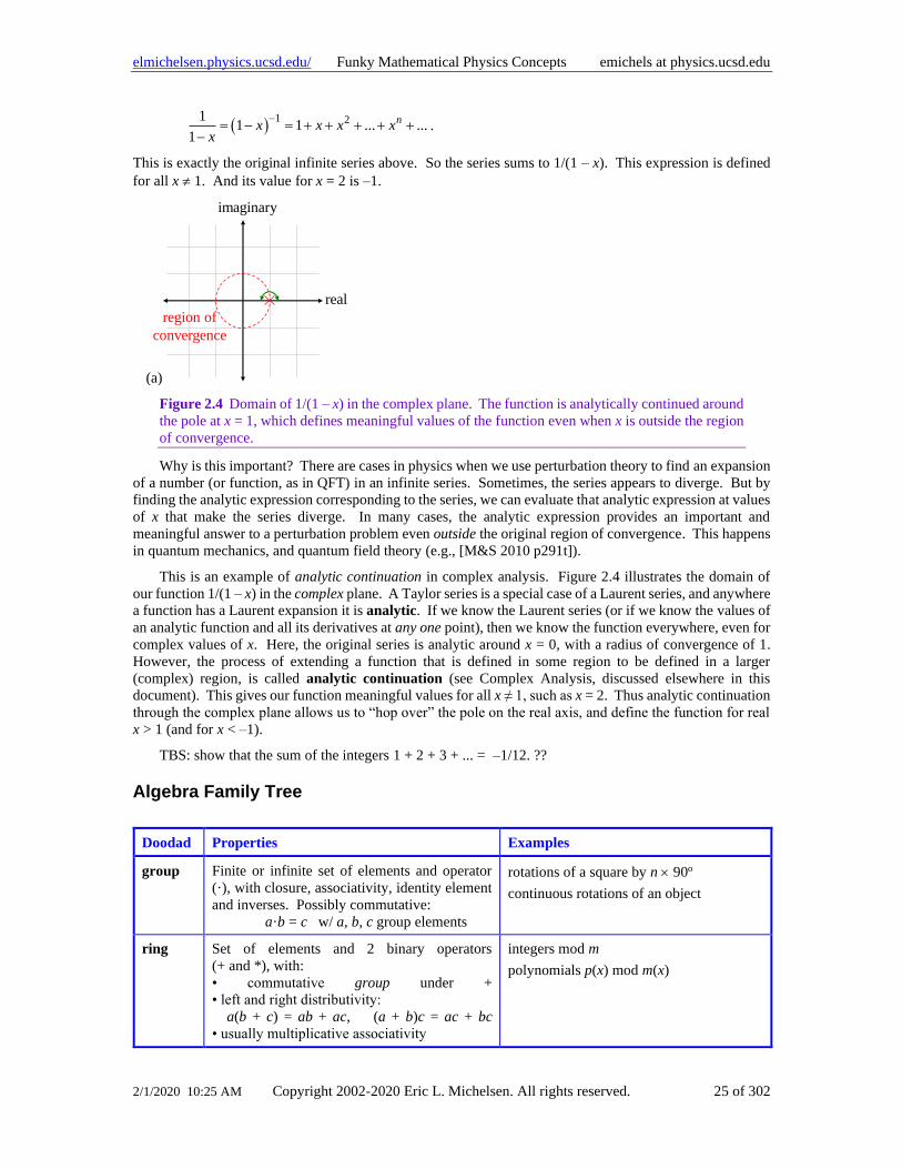
Notice that for integer n > 0, there are n+1 terms. For fractional or negative n, we get an infinite series.
Example 1: Find the Taylor series expansion of 1
1 x−. Since the Taylor series is unique, any method
we use to find a power series expansion will give us the Taylor series. So we can use the binomial theorem,
and apply the rules above, with a = 1, b = (–x):
( )( )( )
( )( )( )
( )( )( )( )
( )1 1 2 31 2 3 4
2
1 1 2 1 2 311 1 1 1 1 ...
1 1 1 2 1 2 3
1 ... ...m
x x x xx
x x x
− − − − −− − − − − −= + − = + − + − + − +
−
= + + + + +
Notice that all the fractions, all the powers of 1, and all the minus signs cancel.
Example 2: Find the Taylor series expansion of ( )1/ 2
1 1x x+ = + . The first term is a1/2 = 11/2:
( )( ) ( ) ( )
( )( )
( )( ) ( )
1/ 2 1/ 2 1/ 2 1 3/ 2 2 5/ 2 3
12 3
1 1 1 1 1 1 1 3 11 1 1 1 1 ...
2 1 2 2 1 2 2 2 2 1 2 3
2 3 !!1 1 31 ... 1
2 8 48 2 !
!! 2 4 ... 2 1
m m
m
x x x x
mx x x x
m
where p p p p or
− − −
+
+ = + + − + − − +
−= + − + − + −
− −
When Does a Divergent Series Converge?
Sometimes, a divergent series “converges.” Consider the infinite series:
21 ... ...
nx x x+ + + + + .
When is it convergent? Apparently, when |x| < 1. What is the value of the series when x = 2 ? “Undefined!”
you say. But there is a very important sense in which the series does converge for x = 2, and it’s value is –
1! How so?
Recall the Taylor expansion around x = 0 (you can use the binomial theorem, see earlier section):
Page 25
elmichelsen.physics.ucsd.edu/ Funky Mathematical Physics Concepts emichels at physics.ucsd.edu
2/1/2020 10:25 AM Copyright 2002-2020 Eric L. Michelsen. All rights reserved. 25 of 302
( )1 21
1 1 ... ...1
nx x x xx
−= − = + + + + +
−.
This is exactly the original infinite series above. So the series sums to 1/(1 – x). This expression is defined
for all x 1. And its value for x = 2 is –1.
real
(a)
imaginary
region of
convergence
Figure 2.4 Domain of 1/(1 – x) in the complex plane. The function is analytically continued around
the pole at x = 1, which defines meaningful values of the function even when x is outside the region
of convergence.
Why is this important? There are cases in physics when we use perturbation theory to find an expansion
of a number (or function, as in QFT) in an infinite series. Sometimes, the series appears to diverge. But by
finding the analytic expression corresponding to the series, we can evaluate that analytic expression at values
of x that make the series diverge. In many cases, the analytic expression provides an important and
meaningful answer to a perturbation problem even outside the original region of convergence. This happens
in quantum mechanics, and quantum field theory (e.g., [M&S 2010 p291t]).
This is an example of analytic continuation in complex analysis. Figure 2.4 illustrates the domain of
our function 1/(1 – x) in the complex plane. A Taylor series is a special case of a Laurent series, and anywhere
a function has a Laurent expansion it is analytic. If we know the Laurent series (or if we know the values of
an analytic function and all its derivatives at any one point), then we know the function everywhere, even for
complex values of x. Here, the original series is analytic around x = 0, with a radius of convergence of 1.
However, the process of extending a function that is defined in some region to be defined in a larger
(complex) region, is called analytic continuation (see Complex Analysis, discussed elsewhere in this
document). This gives our function meaningful values for all x ≠ 1, such as x = 2. Thus analytic continuation
through the complex plane allows us to “hop over” the pole on the real axis, and define the function for real
x > 1 (and for x < –1).
TBS: show that the sum of the integers 1 + 2 + 3 + ... = –1/12. ??
Algebra Family Tree
Doodad Properties Examples
group Finite or infinite set of elements and operator
(·), with closure, associativity, identity element
and inverses. Possibly commutative:
a·b = c w/ a, b, c group elements
rotations of a square by n 90o
continuous rotations of an object
ring Set of elements and 2 binary operators
(+ and *), with:
• commutative group under +
• left and right distributivity:
a(b + c) = ab + ac, (a + b)c = ac + bc
• usually multiplicative associativity
integers mod m
polynomials p(x) mod m(x)
Page 26
elmichelsen.physics.ucsd.edu/ Funky Mathematical Physics Concepts emichels at physics.ucsd.edu
2/1/2020 10:25 AM Copyright 2002-2020 Eric L. Michelsen. All rights reserved. 26 of 302
integral
domain,
or
domain
A ring, with:
• commutative multiplication
• multiplicative identity (but no inverses)
• no zero divisors ( cancellation is valid):
ab = 0 only if a = 0 or b = 0
integers
polynomials, even abstract polynomials,
with abstract variable x, and coefficients
from a “field”
field “rings with multiplicative inverses (& identity)”
• commutative group under addition
• commutative group (excluding 0) under
multiplication.
• distributivity, multiplicative inverses
Allows solving simultaneous linear equations.
Field can be finite or infinite
integers with arithmetic modulo 3 (or any
prime)
real numbers
complex numbers
vector
space
• field of scalars
• group of vectors under +.
Allows solving simultaneous vector equations
for unknown scalars or vectors.
Finite or infinite dimensional.
physical vectors
real or complex functions of space: f(x, y, z)
kets (and bras)
Hilbert
space
vector space over field of complex numbers
with:
• a conjugate-bilinear inner product,
<av|bw> = (a*)b<v|w>,
<v|w> = <w|v>*
a, b scalars, and v, w vectors
• Mathematicians require it to be infinite
dimensional; physicists don’t.
real or complex functions of space: f(x, y, z)
quantum mechanical wave functions
Convoluted Thinking
Convolution arises in many physics, engineering, statistics, and other mathematical areas. As examples,
we here consider functions of time, but the concept of convolution may apply to functions of space, or
anything else. Given two functions, f(t) and g(t), the convolution of f(t) and g(t) is a function of a time-
displacement, Δt, defined by (Figure 2.5):
( )* ( ) ( ) ( ) the integral covers some domain of interestf g t d f g t where
− − .
f(t)
t t
g(t)
τ
increasing Δt
g(Δt1-τ)
f(τ)
Δt1
( f *g)(Δt1)τ
g(Δt2-τ)
f(τ)
Δt2
( f *g)(Δt2)τ
g(Δt0-τ)f(τ)
Δt0 < 0
( f *g)(Δt0)
(a)
(b) (c) (d)
Figure 2.5 (a) Two functions, f(t) and g(t). (b) (f *g)(Δt0), Δt0 < 0. (c) (f *g)(Δt1), Δt1 > 0.
(d) f*g)(Δt2), Δt2 > Δt1. The convolution is the magenta shaded area.
Page 27
elmichelsen.physics.ucsd.edu/ Funky Mathematical Physics Concepts emichels at physics.ucsd.edu
2/1/2020 10:25 AM Copyright 2002-2020 Eric L. Michelsen. All rights reserved. 27 of 302
When Δt < 0, the two functions are “backing into each other” (above left). When Δt > 0, the two functions
are “backing away from each other” (above middle and right).
As noted at the beginning, convolution is useful with a variety of independent variables besides time.
E.g., for functions of space, f(x) and g(x), f *g(Δx) is a function of spatial displacement, Δx.
Notice that convolution is
(1) commutative: * *f g g f=
(2) linear in each of the two functions:
( ) ( )
( )
* * * , and
* * * .
f kg k f g kf g
f g h f g f h
= =
+ = +
The verb “to convolve” means “to form the convolution of.” We convolve f and g to form the convolution
f *g. Some references use “” for convolution: f g.
Two Dimensional Convolution: Impulsive Behavior
A translation invariant linear system (TILS) is completely described by its impulse response. For
example, for small angles, equivalent to narrow fields of view, an optical imaging system is approximately a
TILS. In optics, the impulse response is called the Point Spread Function, or PSF. To illustrate the use of
convolution in a TILS, consider an optical imager (Figure 2.6).
Optical imager (TILS)
u
v
object image x, u
y
(a) (b) image
(x, y)y, vx
Figure 2.6 (a) Optical imager is a TILS. (b) Example image of 3 point sources, with a representative
image point. Each source is spread out by the imager according to the PSF. The red arrow is the
vector (x – u).
The imager has finite resolution, so a point object is spread over a region in the image. For a point object
at the origin with intensity O, the image has intensity distributed over space according to:
( , ) ( , )I x y O PSF x y= .
x and y are position coordinates, such as meters or microradians. We define the object coordinates (u, v) to
be those of their image points (so we can ignore magnification). Then translation invariance says that for a
point object at (u, v):
( , ) ( , )I x y O PSF x u y v= − − .
For incoherent sources, intensities add, so multiple point sources produce an image intensity that is the sum
of the individual images (Figure 2.6b). Therefore, the PSF is real, and represents the intensity response
function (rather than field amplitude). At each point on the image (x, y):
1 1 1 2 2 2 3 3 3
3
1
( , ) ( , ) ( , ) ( , )
( , )i i
i
I x y O PSF x u y v O PSF x u y v O PSF x u y v
PSF x u y v
=
= − − + − − + − −
= − −
For a continuous object, each infinitesimal region of size (du, dv) around each point (u, v) is essentially a
point source. The image is the infinite sum of images of all these “point” sources. Then the sum above
becomes a continuous integral:
Page 28
elmichelsen.physics.ucsd.edu/ Funky Mathematical Physics Concepts emichels at physics.ucsd.edu
2/1/2020 10:25 AM Copyright 2002-2020 Eric L. Michelsen. All rights reserved. 28 of 302
object( , ) ( , ) ( , )I x y du dv O u v PSF x u y v O PSF= − − . (2.4)
This is the definition of a 2D convolution. Some references use “*” for convolution: O*PSF.
In general, for a TILS:
A convolution is an infinite sum of responses to a continuous input.
Translation invariant linear systems are fully described by their impulse response (aka PSF). The
output of such a system is the convolution of the input with the PSF.
All of the above is true for arbitrary PSF, symmetric or not. Some systems exhibit symmetry, e.g. many
optical systems are axially symmetric. In such a symmetric case, the arguments to the PSF may be negated,
though we find such expressions misleading.
For coherent systems, the PSF is generally complex, and it denotes the magnitude and phase of the light
at the image relative to the object. Such a PSF represents the field amplitude response function (rather than
intensity).
In vector notation, the convolution (2.4) can be written:
2
object( ) ( ) ( )I d u O PSF O PSF= − x u x u .
Structure Functions
The term “correlation” has two distinct meanings, both of which are used in astronomy: (1) correlation
between random variables, and (2) correlation between functions (of space or of time). In both meanings,
correlations are used to compare two things. For example, we might compare light, as a function of time, at
point A in space with that at point B, i.e. IA(t) compared to IB(t). If these intensities vary randomly in time,
we might ask, how are the two related?
Correlations between random variables: The correlation of two random variables (RVs) describes
to what extent the two RVs are linearly related to each other. The correlation is quantified with a correlation
coefficient ρ, where ρ = 1 means the two RVs are actually identical. ρ is proportional to the covariance of
the RVs. Two uncorrelated RVs have no linear relationship (though they may be related in other ways), and
ρ = 0. (See Funky Mathematical Physics Concepts for details.)
In many systems, there are an infinite number of RVs, one at each point in space. For example, above a
telescope, at each atmospheric space point x, there may be a randomly-varying temperature T(t, x), index of
refraction N(t, x), or optical phase ϕ(t, x). The variations are over time. It is common that there are
correlations between the RVs at different points in space. For two very nearby points, ρ is near 1: the two
RVs are almost identical. For far separations, ρ is near 0, because the two RVs are essentially unrelated. In
general, at two points x1 and x2, and near some time t0, using optical phase as an example, the two-point
structure function is [Quirr eq. 1]:
0
0
2 21 2 1 2 1 2
~seconds( , ) ( , ) ( , ) ( , ) ( , )
t T
tTD t t dt t t
+
− −x x x x x x .
The averaging duration is of the order of the exposure time, typically some seconds [Fried 1966 Sec III-IV].
The weather typically changes much slower, of order at least minutes. For translation invariant, isotropic
systems, the above depends only on the spatial distance r ≡ |x1 - x2|. This defines a structure function of a
single variable, the distance r:
21 1
~seconds( ) ( ) ( )
TD r − +x x r .
Since the system is translation invariant, Dϕ can be evaluated at any choice of x1. Because the system is
isotropic, Dϕ can be evaluated at any r such that |r| = r.
Page 29
elmichelsen.physics.ucsd.edu/ Funky Mathematical Physics Concepts emichels at physics.ucsd.edu
2/1/2020 10:25 AM Copyright 2002-2020 Eric L. Michelsen. All rights reserved. 29 of 302
A structure function D(r) gives the correlation (linear relationship) for a time-varying physical
quantity between two space points separated by a distance r.
Correlation Functions
The correlation between two functions is a measure of how linearly related they are. The functions are
often functions of time, or functions of space. A measure of their linear relationship is given by the integral
of their product:
3
volume
( ) ( ) or
( ) ( ) or ( ) ( ) .
fg
fg fg
C dt f t g t
C dx f x g x C d f g
−
−
x x x
It is often useful to compare the two function with some offset in one of them. Then the correlation is a
function of this offset:
3
volume( ) ( ) ( ) or ( ) ( ) ( )fg fgC dt f t g t C d x f g
− + + r x r x .
For two unrelated zero-mean functions, the correlation function is zero.
It is frequently useful to compute the correlation of a function with an offset version of itself, called the
autocorrelation function. For example, at a fixed instant in time, consider the temperature variations
throughout the 3D atmosphere, T(x). Then:
3
volume( ) ( ) ( )TTC d x T T +r x r x .
We expect that nearby temperatures are similar, and that distant temperatures are unrelated. Since T(x) is
zero-mean, we expect the autocorrelation function to be large for small offset, and small for large offset. The
distance at which the autocorrelation becomes small is a measure of the size of atmospheric volumes with
similar temperature. A 2D or higher autocorrelation function is not necessarily isotropic. For example, the
temperature may vary differently in the vertical direction than in horizontal ones.
References
[Fried 1966] D. L. Fried, “Optical Resolution Through a Randomly Inhomogeneous Medium for Very
Long and Very Short Exposures,” Journal of the Optical Society of America, Volume 56,
Number 10 October 1966, p1372.
[Quirr] Andreas Quirrenbach, “The Effects of Atmospheric Turbulence on Astronomical
Observations,” unpublished,
https://pdfs.semanticscholar.org/d6bc/66a77fdabd708e06c6c61fc96f6647101920.pdf,
retrieved 2020-01-25.
Page 30
elmichelsen.physics.ucsd.edu/ Funky Mathematical Physics Concepts emichels at physics.ucsd.edu
2/1/2020 10:25 AM Copyright 2002-2020 Eric L. Michelsen. All rights reserved. 30 of 302
3 Vectors
Small Changes to Vectors
Projection of a Small Change to a Vector Onto the Vector
rdr
dr
dr ≡ d|r|
r'r
ˆ' 'r− − r r r r
r − r'
ˆ'r r
r ≡ |r|
(Left) A small change to a vector, and its projection onto the vector.
(Right) Approximate magnitude of the difference between a big and small vector.
It is sometimes useful (in orbital mechanics, for example) to relate the change in a vector to the change
in the vector’s magnitude. The diagram above (left) leads to a somewhat unexpected result:
ˆ ˆ(multiplying both sides by and using )d dr or r r
d r dr
= =
=
r r r r
r r
And since this is true for any small change, it is also true for any rate of change (just divide by dt):
r r =r r
Vector Difference Approximation
It is sometimes useful to approximate the magnitude of a large vector minus a small one. (In
electromagnetics, for example, this is used to compute the far-field from a small charge or current
distribution.) The diagram above (right) shows that:
ˆ' ' , '− − r r r r r r r
Why (r, θ, ) Are Not the Components of a Vector
(r, θ, ) are parameters of a vector, but not components. That is, the parameters (r, θ, ) uniquely define
the vector, but they are not components, because you can’t add them. This is important in much physics, e.g.
involving magnetic dipoles (ref Jac problem on mag dipole field). Components of a vector are defined as
coefficients of basis vectors. For example, the components v = (x, y, z) can multiply the basis vectors to
construct v:
ˆ ˆ ˆx y z= + +v x y z
There is no similar equation we can write to construct v from it’s spherical components (r, θ, ). Position
vectors are displacements from the origin, and there are no ˆˆ ˆ, ,r θ φ defined at the origin.
Put another way, you can always add the components of two vectors to get the vector sum:
( ) ( ) ( )ˆ ˆ ˆ( , , ) rectangular components.Let a b c Then a x b y c z= + = + + + + +w v w x y z
We can’t do this in spherical coordinates:
( )( , , ) spherical components. , ,w w w v w v w v wLet r Then r r = + + + +w v w
However, at a point off the origin, the basis vectors ˆˆ ˆ, ,r θ φ are well defined, and can be used as a basis
for general vectors. [In differential geometry, vectors referenced to a point in space are called tangent
Page 31
elmichelsen.physics.ucsd.edu/ Funky Mathematical Physics Concepts emichels at physics.ucsd.edu
2/1/2020 10:25 AM Copyright 2002-2020 Eric L. Michelsen. All rights reserved. 31 of 302
vectors, because they are “tangent” to the space, in a higher dimensional sense. See Differential Geometry
elsewhere in this document.]
Laplacian’s Place
What is the physical meaning of the Laplacian operator? And how can I remember the Laplacian
operator in any coordinates? These questions are related because understanding the physical meaning allows
you to quickly derive in your head the Laplacian operator in any of the common coordinates.
Let’s take a step-by-step look at the action of the Laplacian, first in 1D, then on a 3D differential volume
element, with physical examples at each step. After rectangular, we go to spherical coordinates, because they
illustrate all the principles involved. Finally, we apply the concepts to cylindrical coordinates, as well. We
follow this outline:
1. Overview of the Laplacian operator
2. 1D examples of heat flow
3. 3D heat flow in rectangular coordinates
4. Examples of physical scalar fields [temperature, pressure, electric potential (2 ways)]
5. 3D differential volume elements in other coordinates
6. Description of the physical meaning of Laplacian operator terms, such as
2 2 2 2, , , ,
T T T TT r r r r
r r r r r r
.
Overview of Laplacian operator: Let the Laplacian act on a scalar field T(r), a physical function of
space, e.g. temperature. Usually, the Laplacian represents the net outflow per unit volume of some physical
quantity: something/volume, e.g., something/m3. The Laplacian operator itself involves spatial second-
derivatives, and so carries units of inverse area, say m–2.
1D Example: Heat Flow: Consider a temperature gradient along a line. It could be a perpendicular
wire through the wall of a refrigerator (Figure 3.1a). It is a 1D system, i.e. only the gradient along the wire
matters.
tem
per
ature
x
metal wire
refrigerator warmer room
tem
per
atu
re
x
current carrying wire
heat flow
heat flow
refrigerator warmer room
(a) (b)
wall wall
Figure 3.1 Heat condition (a) in a passive wire, and (b) in a heat-generating wire.
Let the left and right sides of the wire be in thermal equilibrium with the refrigerator and room, at 2 C
and 27 C, respectively. The wire is passive, and can neither generate nor dissipate heat; it can only conduct
it. Let the 1D thermal conductivity be k = 100 mW-cm/C. Consider the part of the wire inside the insulated
wall, 4 cm thick. How much heat (power, J/s or W) flows through the wire?
( )25
100 mW-cm/C 625 mW4 cm
dT CP k
dx= = = .
Page 32
elmichelsen.physics.ucsd.edu/ Funky Mathematical Physics Concepts emichels at physics.ucsd.edu
2/1/2020 10:25 AM Copyright 2002-2020 Eric L. Michelsen. All rights reserved. 32 of 302
There is no heat generated or dissipated in the wire, so the heat that flows into the right side of any
segment of the wire (differential or finite) must later flow out the left side. Thus, the heat flow must be
constant along the wire. Since heat flow is proportional to dT/dx, dT/dx must be constant, and the temperature
profile is linear. In other words, (1) since no heat is created or lost in the wire, heat-in = heat-out; (2) but
heat flow ~ dT/dx; so (3) the change in the temperature gradient is zero:
2
20
d dT d T
dx dx dx
= =
.
(At the edges of the wall, the 1D approximation breaks down, and the inevitable nonlinearity of the
temperature profile in the x direction is offset by heat flow out the sides of the wire.)
Now consider a current carrying wire which generates heat all along its length from its resistance (Figure
3.1b). The heat that flows into the wire from the room is added to the heat generated in the wire, and the sum
of the two flows into the refrigerator. The heat generated in a length dx of wire is
2 2resistance per unit length, andgenP I dx where I const = = .
In steady state, the net outflow of heat from a segment of wire must equal the heat generated in that segment.
In an infinitesimal segment of length dx, we have heat-out = heat-in + heat-generated:
2
2
22 2
2
out in gena a dx
a dx a
dT dTP P P I dx
dx dx
dT dTI dx
dx dx
d dT d Tdx I dx I
dx dx dx
+
+
= + = +
− = −
= − = −
The negative sign means that when the temperature gradient is positive (increasing to the right), the heat
flow is negative (to the left), i.e. the heat flow is opposite the gradient. Many physical systems have a similar
negative sign. Thus the 2nd derivative of the temperature is the negative of heat outflow (net inflow) from a
segment, per unit length of the segment. Longer segments have more net outflow (generate more heat).
3D Rectangular Volume Element
Now consider a 3D bulk resistive material, carrying some current. The current generates heat in each
volume element of material. Consider the heat flow in the x direction, with this volume element:
dxx
y
z
Outflow surface area
is the same as inflow flow
The temperature gradient normal to the y-z face drives a heat flow per unit area, in W/m2. For a net flow to
the right, the temperature gradient must be increasing in magnitude (becoming more negative) as we move
to the right. The change in gradient is proportional to dx, and the heat outflow flow is proportional to the
area, and the change in gradient:
2
2
out inout in
P Pd dT d TP P k dx dy dz k
dx dx dx dy dz dx
− − = − = −
.
Thus the net heat outflow per unit volume, due to the x contribution, goes like the 2nd derivative of T.
Clearly, a similar argument applies to the y and z directions, each also contributing net heat outflow per unit
Page 33
elmichelsen.physics.ucsd.edu/ Funky Mathematical Physics Concepts emichels at physics.ucsd.edu
2/1/2020 10:25 AM Copyright 2002-2020 Eric L. Michelsen. All rights reserved. 33 of 302
volume. Therefore, the total heat outflow per unit volume from all 3 directions is simply the sum of the heat
flows in each direction:
2 2 2
2 2 2
out inP P T T Tk
dx dy dz x y z
− = − + +
.
We see that in all cases, the
net outflow of flux per unit volume = change in (flux per unit area), per unit distance
We will use this fact to derive the Laplacian operator in spherical and cylindrical coordinates.
General Laplacian
We now generalize. For the Laplacian to mean anything, it must act on a scalar field whose gradient
drives a flow of some physical thing.
Example 1: My favorite is T(r) = temperature. Then T(r) drives heat (energy) flow, heat per unit
time, per unit area:
/( )
heat tk T where k thermal conductivity
area
heat flow vector
= −
q r
q
Then ~ r
Tq radial component of heat flow
r
=
Example 2: T(r) = pressure of an incompressible viscous fluid (e.g. honey). Then T(r) drives fluid
mass (or volume) flow, mass per unit time, per unit area:
/( )
mass tk T where k some viscous friction coefficient
areamass flow density vector
= −
j r
j
Then ~ r
Tj radial component of mass flow
r
=
Example 3: T(r) = electric potential in a resistive material. Then T(r) drives charge flow, charge per
unit time, per unit area:
charge /( )
tT where electrical conductivity
areacurrent density vector
= −
j r
j
Then ~ r
Tj radial component of current density
r
=
.
Example 4: Here we abstract a little more, to add meaning to the common equations of
electromagnetics. Let T(r) = electric potential in a vacuum. Then T(r) measures the energy per unit
distance, per unit area, required to push a fixed charge density ρ through a surface, by a distance of dn, normal
to the surface:
energy/distance( ) electric charge volume densityT where
area r .
Then ∂T/∂r ~ net energy per unit radius, per unit area, to push charges of density ρ out the same distance
through both surfaces.
Page 34
elmichelsen.physics.ucsd.edu/ Funky Mathematical Physics Concepts emichels at physics.ucsd.edu
2/1/2020 10:25 AM Copyright 2002-2020 Eric L. Michelsen. All rights reserved. 34 of 302
In the first 3 examples, we use the word “flow” to mean the flow in time of some physical quantity, per
unit area. In the last example, the “flow” is energy expenditure per unit distance, per unit area. The
requirement of “per unit area” is essential, as we soon show.
Laplacian In Spherical Coordinates
To understand the Laplacian operator terms in other coordinates, we need to take into account two
effects:
1. The outflow surface area may be different than the inflow surface area
2. The derivatives with respect to angles (θ or ) need to be converted to rate-of-change per unit
distance.
We’ll see how these two effects come into play as we develop the spherical terms of the Laplacian operator.
The cylindrical terms are simplifications of the spherical terms.
Spherical radial contribution: We first consider the radial contribution to the spherical Laplacian
operator, from this volume element:
drx
y
z
θ
Outflow surface area
is differentially
larger than inflow
flow
dΩ
sin θ ddθ
dΩ = sin θ d dθ
The differential volume element has thickness dr, which can be made arbitrarily small compared to the
lengths of the sides. The inner surface of the element has area r2 d. The outer surface has infinitesimally
more area. Thus the radial contribution includes both the “surface-area” effect, but not the “converting-
derivatives” effect.
The increased area of the outflow surface means that for the same flux-density (flow) on inner and outer
surfaces, there would be a net outflow of flux, since flux = (flux-density)(area). Therefore, we must take the
derivative of the flux itself, not the flux density, and then convert the result back to per-unit-volume. We do
this in 3 steps:
( )( ) ( )
( )( )
( )
( )( ) ( )
2
2
2 2
2 2
flux area flux-density ~
flux
fluxoutflow 1 1
volume area
r dr
dr d
dr r r
dr d r
dr r r r rr d r
=
=
= = =
The constant d factor from the area cancels when converting to flux, and back to flux-density. In other
words, we can think of the fluxes as per-steradian.
We summarize the stages of the spherical radial Laplacian operator as follows:
Page 35
elmichelsen.physics.ucsd.edu/ Funky Mathematical Physics Concepts emichels at physics.ucsd.edu
2/1/2020 10:25 AM Copyright 2002-2020 Eric L. Michelsen. All rights reserved. 35 of 302
2 2
2
2
2
2
1( ) ( )
radial flux per unit area
( )( )radial flux, per unit solid-angle
change in radial flux per unit length, per unit solid-angle; positive is increasing flux
1
r T r Tr rr
Tr
area flow per unit arear T
r d
r Tr r
r
=
=
= =
=
r r
2
2
2
radial flowper unit area
radial fluxper steradian
change in radial flux perunit length per steradian
change in radial flux per unit length, per unit area
net outflow of flux per unit volume
1
r Tr r
r Tr rr
=
=
change in radial flux perunit length, per unit area
Following the steps in the example of heat flow, let T(r) = temperature. Then
2
2
2
2
2
radial heat flow per unit area, W/m
Wattsradial heat flux, W/solid-angle =
steradian
change in radial heat flux per unit length, per unit solid-angle
1net outflow of heat flux per unit volume
Tr
r Tr
r Tr r
r Tr rr
=
=
=
=
Spherical azimuthal contribution: The spherical contribution to the Laplacian has no area-change,
but does require converting derivatives. Consider the volume element:
d
Outflow surface area
is identical to inflow
x
y
z
θ
flow
The inflow and outflow surface areas are the same, and therefore area-change contributes nothing to the
derivatives.
However, we must convert the derivatives with respect to into rates-of-change with respect to distance,
because physically, the flow is driven by a derivative with respect to distance. In the spherical case, the
effective radius for the arc-length along the flow is r sin θ, because we must project the position vector into
the plane of rotation. Thus, (∂/∂) is the rate-of-change per (r sin θ) meters. Therefore,
1rate-of-change-per-meter
sinr
=
Page 36
elmichelsen.physics.ucsd.edu/ Funky Mathematical Physics Concepts emichels at physics.ucsd.edu
2/1/2020 10:25 AM Copyright 2002-2020 Eric L. Michelsen. All rights reserved. 36 of 302
Performing the two derivative conversions, we get
2 1 1( ) ( )
sin sin
1azimuthal flux per unit area
sin
1change in (azimuthal flux per unit area) per radian
sin
1 1change in (azimuthal flux per unit area) per unit distance
sin sin
net azimu
T Tr r
Tr
Tr
Tr r
=
=
=
=
=
r r
azimuthal fluxper unit area
change in (azimuthal fluxper unit area) per radian
change in (azimuthal flux perunit area) per unit distance
thal outflow of flux per unit volume
1 1
sin sinT
r r
2
2 2 2
1
sinT
r
=
Notice that the r2 sin2 θ in the denominator is not a physical area; it comes from two derivative
conversions.
Spherical polar angle contribution:
dθ
Outflow surface area
is differentially
larger than inflow
x
y
z
θ
flow
The volume element is like a wedge of an orange: it gets wider (in the northern hemisphere) as θ
increases. Therefore the outflow area is differentially larger than the inflow area (in the northern
hemisphere). In particular, ( )sinarea r dr= , but we only need to keep the θ dependence, because the
factors of r cancel, just like d did in the spherical radial contribution. So we have
sinarea .
In addition, we must convert the ∂/∂θ to a rate-of-change with distance. Thus the spherical polar angle
contribution has both area-change and derivative-conversion.
Following the steps of converting to flux, taking the derivative, then converting back to flux-density, we
get
Page 37
elmichelsen.physics.ucsd.edu/ Funky Mathematical Physics Concepts emichels at physics.ucsd.edu
2/1/2020 10:25 AM Copyright 2002-2020 Eric L. Michelsen. All rights reserved. 37 of 302
( )
2 1 1 1( ) sin ( )
sin
1 ˆ-flux per unit area
( )( )1 ˆsin -flux, per unit radius
1 ˆsin change in -flux per unit radius , per radian
1 1 ˆsin change in -flux per
T Tr r
Tr
area flux per unit areaT
r dr
Tr
Tr r
=
=
= =
=
=
r r
( )
ˆ-flux perunit area
ˆ-flux, perunit radius
change
unit radius , per unit distance
1 1 1 ˆsin change in ( -flux per unit area), per unit distancesin
net outflow of flux per unit volume
1 1 1sin
sin
Tr r
Tr r
=
=
2
ˆin ( -flux perunit radius), per radian
ˆchange in ( -flux per unitradius), per unit distance
ˆchange in ( -flux per unitarea), per unit distance
1sin
sinT
r
=
Notice that the r2 in the denominator is not a physical area; it comes from two derivative conversions.
Cylindrical Coordinates
The cylindrical terms are simplifications of the spherical terms.
drx
y
z
Radial outflow
surface area is
differentially larger
than inflow
flow
r
d
flow
and z outflow
surface areas are
identical to
inflow dz
flow
Cylindrical radial contribution: The picture of the cylindrical radial contribution is essentially the
same as the spherical, but the “height” of the slab is exactly constant. We still face the issues of varying
inflow and outflow surface areas, and converting derivatives to rate of change per unit distance. The change
in area is due only to the arc length r d, with the z (height) fixed. Thus we write the radial result directly:
Page 38
elmichelsen.physics.ucsd.edu/ Funky Mathematical Physics Concepts emichels at physics.ucsd.edu
2/1/2020 10:25 AM Copyright 2002-2020 Eric L. Michelsen. All rights reserved. 38 of 302
2 1( ) ( ) (Cylindrical Coordinates)
radial flow per unit area
(flow per unit area)(area)radial flux per unit angle
change in (radial flux per unit angle), per unit radius
1change i
r T r Tr r r
Tr
r Tr d dz
r Tr r
r Tr r r
=
=
= =
=
=
r r
radial flowper unit area
radial fluxper radian
change in radial flux perunit length per radian
change in (radial flux pe
n (radial flux per unit area), per unit radius
net outflow of flux per unit volume
1r T
r r r
=
runit area), per unit radius
Cylindrical azimuthal contribution: Like the spherical case, the inflow and outflow surfaces have
identical areas. Therefore, the contribution is similar to the spherical case, except there is no sin θ factor;
r contributes directly to the arc-length and rate-of-change per unit distance:
( )
2 1 1( ) ( )
1azimuthal flux per unit area
1change in azimuthal flux per unit area per radian
1 1change in (azimuthal flux per unit area) per unit distance
net azimuthal outflow of flux per unit vo
T Tr r
Tr
Tr
Tr r
=
=
=
=
=
r r
2
2 2
change in (azimuthal flux perunit area) per unit distance
lume
1 1 1
azimuthal flowper unit area
change in azimuthalflow per radian
T Tr r r
=
Cylindrical z contribution: This is identical to the rectangular case: the inflow and outflow areas are
the same, and the derivative is already per unit distance, ergo: (add cylindrical volume element picture??)
Page 39
elmichelsen.physics.ucsd.edu/ Funky Mathematical Physics Concepts emichels at physics.ucsd.edu
2/1/2020 10:25 AM Copyright 2002-2020 Eric L. Michelsen. All rights reserved. 39 of 302
2
vertical fluxper unit area
change in (vertical flux perunit area) pe
( ) ( )
vertical flux per unit area
change in (vertical flux per unit area) per unit distance
net outflow of flux per unit volume
zT Tz z
Tz
Tz z
Tz z
=
=
=
=
r r
2
2
r unit distance
Tz
=
Laplacian of a Vector Field
It gets worse: there’s a vector form of 2. If E(x, y, z) is a vector field, then in rectangular coordinates:
2 2 2 2x y zE E E = + + E E i j k .
This arises in E&M propagation, and not much in QM. However, the above equality is only true in
rectangular coordinates [I have a ref for this, but lost it??]. This is the divergence of the gradient of a vector
field, which is a vector. In oblique or non-normal coordinates, the gradient and divergence must be covariant,
and include the Christoffel symbols.
Vector Dot Grad Vector
In electromagnetic propagation, and elsewhere, one encounters the “dot product” of a vector field with
the gradient operator, acting on a vector field. What is this v · operator? Here, v(r) is a given vector field.
The simple view is that v(r) · is just a notational shorthand for
( )
( ) ,
ˆ ˆ ˆ ˆ ˆ ˆ( )
x y z
x y z x y z
v v vx y z
because v v v v v vx y z x y z
+ +
= + + + + = + +
v r
v r x y z x y z
by the usual rules for a dot product in rectangular coordinates.
There is a deeper meaning, though, which is an important bridge to the topics of tensors and differential
geometry.
We can view the v · operator as simply the dot product of the vector field v(r)
with the gradient of a vector field.
You may think of the gradient operator as acting on a scalar field, to produce a vector field. But the
gradient operator can also act on a vector field, to produce a tensor field. Here’s how it works: You are
probably familiar with derivatives of a vector field:
Page 40
elmichelsen.physics.ucsd.edu/ Funky Mathematical Physics Concepts emichels at physics.ucsd.edu
2/1/2020 10:25 AM Copyright 2002-2020 Eric L. Michelsen. All rights reserved. 40 of 302
ˆ ˆ ˆ( , , ) be a vector field. Then is a vector field.
Writing spatial vectors as column vectors, ,
Similarly, are
yx z
x
xy
y
zz
AA ALet x y z
x x x x
A
xA
AA A and
x xA A
x
andy z
= + +
= =
AA x y z
A
A Aalso vector fields.
By the rule for total derivatives, for a small displacement (dx, dy, dz),
x x
y
x x
xy y
z
x
y y
zz zz
z
y
A
z
A
dxA A
x xdA
A Adx dx
x x
A
A A
y y
A AdydA dy
y y
A AA
y xx
dzy
dAA dz
z y
dx y z
= + + = = +
A A AA
x
y
z
A
z
Adz
y
A
z
dy
+
.
This says that the vector dA is a linear combination of 3 column vectors ∂A/∂x, ∂A/∂y, and ∂A/∂z, weighted
respectively by the displacements dx, dy, and dz. The 3 x 3 matrix above is the gradient of the vector field
A(r). It is the natural extension of the gradient (of a scalar field) to a vector field. It is a rank-2 tensor, which
means that given a vector (dx, dy, dz), it produces a vector (dA) which is a linear combination of 3 (column)
vectors (A), each weighted by the components of the given vector (dx, dy, dz).
Note that A and ·A are very different: the former is a rank-2 tensor field, the latter is a scalar field.
This concept extends further to derivatives of rank-2 tensors, which are rank-3 tensors: 3 x 3 x 3 cubes
of numbers, producing a linear combination of 3 x 3 arrays, weighted by the components of a given vector
(dx, dy, dz). And so on.
Note that in other coordinates (e.g., cylindrical or spherical), A is not given by the derivative of its
components with respect to the 3 coordinates. The components interact, because the basis vectors also change
through space. That leads to the subject of differential geometry, discussed elsewhere in this document.
Page 41
elmichelsen.physics.ucsd.edu/ Funky Mathematical Physics Concepts emichels at physics.ucsd.edu
2/1/2020 10:25 AM Copyright 2002-2020 Eric L. Michelsen. All rights reserved. 41 of 302
4 Green Functions
We follow [Jac p??] and [Bra] in using the term “Green function,” rather than “Green’s function.”
Though we agree with Jackson’s logic, we do it mostly because it’s easier to say and type.
Green functions are a big topic, with lots of subtopics. Many references describe only a subset, but use
words that imply they are covering all of Green functions. If you are looking for a specific application of
Green functions, such as electrostatics, you may want to skip right to that section, but the “big idea” applies
to all Green functions.
Though Green functions are used to solve linear operator equations (such as differential equations), the
concepts involved apply to other applications, such as the Born approximation, impulse response analysis,
and quantum propagators.
The Big Idea
Green functions are a method of solving linear operator equations (such as inhomogeneous linear
differential equations) of the form:
source
( ) ( ) is a linear operatorf x s x where=L L . (4.1)
s(x) is called the “source” function. We use Green functions when other methods are hard, or to make a
useful approximation (the Born approximation). The big idea is to break up the source s(x) into infinitesimal
pieces (δ-functions), solve each piece separately, and add up the solutions. Since the is linear, the sum of
solutions is also a solution, and is the solution to the original problem.
Sometimes, the Green function itself can be given physical meaning, as in E&M where it is essentially
Huygen’s Principle, but with accurate phase information, or in Quantum Field Theory where it is the
propagator of a quantized field. Green functions can generate particular (i.e. inhomogeneous) solutions, and
solutions matching boundary conditions. They don’t generate homogeneous solutions (i.e., where the right
hand side is zero). We explore Green functions through the following steps:
1. Extremely brief review of the δ-function.
2. The tired, but inevitable, electromagnetic example.
3. Linear differential equations of one variable (1-dimensional), with sources.
4. Delta function expansions.
5. Green functions of two variables (but 1 dimension).
6. When you can collapse a Green function to one variable (“portable Green functions”: translational
invariance)
7. Dealing with boundary conditions: at least 5 (6??) kinds of BC
8. Green-like methods: the Born approximation
You will find no references to “Green’s Theorem” or “self-adjoint” until we get to non-homogeneous
boundary conditions, because until then, those topics are unnecessary and confusing. We will see that:
The biggest hurdle in understanding Green functions is the boundary conditions.
Some references derive Green functions from Green’s Theorem, which derives from Gauss’ Law.
That is only a special case. In general, Green functions do not rely on Green’s Theorem.
We return to this point later, after discussing general boundary conditions.
Dirac Delta Function
Recall that the Dirac δ-function is an “impulse,” an infinitely narrow, tall spike function, defined as:
Page 42
elmichelsen.physics.ucsd.edu/ Funky Mathematical Physics Concepts emichels at physics.ucsd.edu
2/1/2020 10:25 AM Copyright 2002-2020 Eric L. Michelsen. All rights reserved. 42 of 302
( ) 0, 0, and ( ) 1, 0 (the area under the -function is 1)a
ax for x x dx a
−= = .
(This also implies (0) → , but we don’t focus on that here.) The linearity of integration implies the delta
function can be offset, and weighted, so that:
( ) 0b a
b aw x b dx w a
+
−− = .
Since the δ-function is infinitely narrow, it can “pick out” a single value from a function:
( ) ( ) ( ) 0b a
b ax b f x dx f b a
+
−− = . (4.2)
This is called the “filtering property” of the δ-function. See Quirky Quantum Concepts for more on the delta
function. The units of δ( ) are [x]–1.
The Tired, But Inevitable, Electromagnetic Example
You probably have seen Poisson’s equation relating the electrostatic potential at a point to the charge
distribution creating the potential (in gaussian units):
2 ( ) 4 ( ) electrostatic potential, charge densitywhere − = r r . (4.3)
We solved this by noting three things: (1a) electrostatic potential, , obeys “superposition:” the potential due to multiple charges is the sum of the potentials of the individual charges; (1b) the potential is proportional to
the source charge; and (2) if we take the potential at infinity to be zero, the potential due to a point charge is:
1( ) (point charge at ')
'q =
−r r
r r. (4.4)
(We say much more about boundary conditions later.) The properties (1a) and (1b) above, taken together,
define a linear relationship:
1 1 2 2
1 2 1 2
Given: ( ') ( ), and ( ') ( ),
then: ( ') ( ') ( ) ( ) ( ) .totala a
→ →
+ → = +
r r r r
r r r r r
To solve (4.3), we break up the source charge distribution ρ(r) into an infinite number of little point
charges. The set of points is spread out over space, each of charge ρ(r) d3r. The solution for is the sum of
potentials from all the point charges, and the infinite sum is an integral, so we find as:
3
# points3 3
' 01
1 1( ) lim ( ' ) ' ( ') '
' 'i
d r ii
d r d r
→=
= =− −
r r rr r r r
.
Note that the charge “distribution” for a point charge is a δ-function: infinite charge density, but finite total
charge. Also, ϕ(r) for a point charge at r’ is translationally invariant: it has the same form for all r’. We will
remove this restriction later.
All of this followed from simple mathematical properties of Eq (1) that have nothing to do with
electromagnetics. All we used to solve for was that the left-hand side is a linear operator on (so
superposition applies), and we have a known solution when the right-hand side is a delta function at r’:
linear linearunknown given "source" given pointoperator operatorfunction function "source" at 'known
solutio
2
n
2 1( ) ( ) and ( ')
' − = − = −
−
r
r r r rr r
.
Page 43
elmichelsen.physics.ucsd.edu/ Funky Mathematical Physics Concepts emichels at physics.ucsd.edu
2/1/2020 10:25 AM Copyright 2002-2020 Eric L. Michelsen. All rights reserved. 43 of 302
Since any given ρ can be written as a sum of weighted δ-functions, the solution for that given ρ is a sum of
delta-function solutions. Now we generalize this electromagnetic example to arbitrary (for now, 1D) linear
operator equations by letting r → x, → f, –2 → , ρ → s, and call the known δ-function solution G(x):
2 2
( ) ( ) given point"source" at '( ')
1( ) ( ) and ( ')
'
Given ( ) ( ) and ( ') ( '),
then ( ) ' ( ') ( ') .
f x s x
G
f x s x G x x x x
f x dx s x G x x
−
−
− = − = − →−
= − = −
= −
rr r
r r r rr r
This assumes, as above, that our linear operator, and any boundary conditions, are translationally invariant.
A Fresh, New Signal Processing Example
If the following example doesn’t make sense to you, just skip it. Signal processing and control theory
folk have long used a Green function-like concept, but with different words. A time-invariant linear system
(TILS) produces an output which is a linear operation on its input:
( ) ( ) is a linear operation taking input to outputo t i t where= .
In this case, we aren’t given {}, and we don’t solve for it (also it’s on the right-, rather than the left-side
of the equation). However, we are given a measurement (or computation) of the system’s impulse response,
called h(t). If you poke the system with a very short spike (i.e., if you feed an impulse into the system, i(t) =
δ(t) ), the system responds with h(t):
( ) ( ) ( ) is the system's impulse responseh t t where h t= .
h(t) acts like a Green function, giving the system response at time t to a delta function at t = 0. Note that h(t)
is spread out over time, and usually of (theoretically) infinite duration. h(t) fully characterizes the system,
because we can express any input function as a series of impulses (with the delta-function expansion below),
and sum up all the responses. Therefore, we find the output for any input, i(t), with:
( ) ( ') ( ') 'o t i t h t t dt
−= − .
Caution: many references do not distinguish between a Green function G(x) and an impulse response
h(x). The two are similar, but they differ because:
( ) ( ), but ( ) ( )G x x h x x = = .
The δ-function is in a different place for a Green function vs. an impulse response. For example, in
electromagnetics, sources (charges and currents) are the stimulus that result in fields (E and B). Maxwell’s
equations have linear operators acting on the result (fields) to give you the stimulus. A TILS does the reverse:
it produces a result which is a linear operation on its input (stimulus).
We can see a relationship between a Green function and an impulse response by taking –1 (if it exists)
of both sides of the second equation:
1 ( ) ( )h x x− = .
Thus the impulse response for an operator is the Green function for the operator –1. In particular,
quantum field theory calls the field “propagator” a Green function, but it is more directly thought-of as an
impulse response.
Page 44
elmichelsen.physics.ucsd.edu/ Funky Mathematical Physics Concepts emichels at physics.ucsd.edu
2/1/2020 10:25 AM Copyright 2002-2020 Eric L. Michelsen. All rights reserved. 44 of 302
Linear differential equations of one variable, with sources
We wish to solve for f(x), given s(x):
2 22 2
2 2
( ) ( ), is a linear operator .
( ) is called the "source," or forcing function .
E.g., ( ) ( ) ( ) ( ) .
f x s x where
s x
d df x f x f x s x
dx dx
=
+ + =
We ignore boundary conditions for now (to be dealt with later). The differential equations often have 3D
space as their domain. Note that we are not differentiating s(x), which will be important when we get to the
delta function expansion of s(x).
Green functions solve the above equation by first solving a related equation: if we can find a function
(i.e., a “Green function”) such that:
22
2
( ) ( ), ( ) is the Dirac delta function,
e.g., ( ) ( ) ,
G x x where x
dG x x
dx
=
+ =
then we can use that Green function to solve our original equation. This might seem weird, because δ(0) →
∞, but it just means that Green functions often have discontinuities in them or their derivatives. For example,
suppose G(x) is a step function:
( ) 0, 0( ) ( )
1, 0Then
G x x dG x x
x dx
= =
= .
Now suppose our source isn’t centered at the origin, i.e., ( ) ( )s x x a= − . If L is translation invariant
[along with any boundary conditions], then G( ) can still solve the equation by translation:
( ) ( ) ( ), ( ) ( ) is a solution.f x s x x a f x G x a= = − = −L
If s(x) is a weighted sum of delta functions at different places, then because L is linear, the solution is
immediate: we just add up the solutions from all the δ-functions:
( ) ( ) ( ) ( ) ( )i i i i
i i
f x s x w x x f x w G x x= = − = − .
Usually the source s(x) is continuous. Then we can break up s(x) into infinitesimally small pieces (i.e.,
expand it as an infinite sum of delta functions, described in a moment), and sum the solutions for the pieces.
The summation goes over to an integral, and a solution is:
'( ') '
1
source source
( ) ( ) ( )
( ) ( ) ( ') ' ( ') and ( ) ' ( ') ( ')
i
i
x xw s x dx
i i
i
f x s x w x x
f x s x s x dx x x f x dx s x G x x
→ →
=
= = − →
= = − = −
We can show directly that f(x) is a solution of the original equation by plugging it in, and noting that
L acts in the x domain, and “goes through” (i.e., commutes with) any operation in x’:
Page 45
elmichelsen.physics.ucsd.edu/ Funky Mathematical Physics Concepts emichels at physics.ucsd.edu
2/1/2020 10:25 AM Copyright 2002-2020 Eric L. Michelsen. All rights reserved. 45 of 302
( ) ' ( ') ( ')
' ( ') ( ') moving inside the integral
' ( ') ( ') ( ) ( ) picks out the value of ( ). .
f x dx s x G x x
dx s x G x x
dx s x x x s x s x QED
= −
= −
= − =
L L
L L
We now digress for a moment to understand the δ-function expansion.
Delta Function Expansion
As in the EM example, it is frequently quite useful to expand a given function s(x) as a sum of δ-
functions:
1
( ) ( ), are the weights of the basis delta functions
N
i i i
i
s x w x x where w
=
− .
[This same expansion is used to characterize the response of linear systems to input i(t).]
x(a)
s(x)
N = 8
x
s(x)
Δxxi
wi = area
≈ s(xi)Δx
N = 16
(b)
Figure 4.1 (a) Approximating a function with δ-functions. (b) The weight of each δ-function is
such that its integral approximates the integral of the given function, s(x), over the interval “covered”
by the δ-function.
In Figure 4.1a, we approximate s(x) first with N = 8 δ-functions (green), then with N = 16 δ-functions (red).
As we double N, the weight of each δ-function is roughly cut in half, but there are twice as many of them.
Hence, the integral of the δ-function approximation remains about the same. Of course, the approximation
gets better as N increases. As usual, we let the number of δ-functions go to infinity: N → ∞.
In Figure 4.1b, we show how to choose the weight of each δ-function: its weight is such that its integral
approximates the integral of the given function, s(x), over the interval “covered” by the δ-function. In the
limit of N → ∞, the approximation becomes arbitrarily good.
In what sense is the δ-function series an approximation to s(x)? Certainly, if we need the derivative s'(x),
the delta function expansion seems to be terrible. However, if we want the integral of s(x), or any integral
operator, such as an inner product or a convolution, then the delta function series is a good approximation.
Examples:
1
For ( ) or ( ) ( ) , or ( ' ) ( ) ,
then ( ) ( ) ( ) .
N
i i i i
i
s x dx f x s x dx f x x s x dx
s x w x x where w s x x
=
−
− =
As N → ∞, we expand s(x) in an infinite sum (an integral) of δ-functions:
Page 46
elmichelsen.physics.ucsd.edu/ Funky Mathematical Physics Concepts emichels at physics.ucsd.edu
2/1/2020 10:25 AM Copyright 2002-2020 Eric L. Michelsen. All rights reserved. 46 of 302
''
( ') '
( ) ( ) ( ) ' ( ') ( ')
i
i
x xx dx
w s x dx
i i
i
s x w x x s x dx s x x x
→ →
→
= − → = − ,
which if you think about it, follows directly from the definition of δ(x), per (4.2).
[Aside: Delta functions are a continuous set of orthonormal basis functions, much like sinusoids from quantum
mechanics and Fourier transforms. They satisfy all the usual orthonormal conditions for a continuous basis, i.e. they
are orthogonal and normalized:
( ) ( ) ( )dx x a x b a b
−− − = − .]
Note that in the final solution of the prior section, we integrate s(x) times other stuff:
( ) ' ( ') ( ')f x dx s x G x x= − ,
and integrating over s(x) is what makes the δ-function expansion of s(x) valid.
[Aside: It turns out that even systems that differentiate s(x) can use the δ-function expansion, but we need not
bother with that here.]
Boundary Conditions on Green Functions
Most problems require boundary conditions on the solution to an equation.
Introduction to Boundary Conditions
We now impose a simple boundary condition on an equation we seek to solve. Consider a 2D problem
in the plane:
( , ) ( , ) inside the boundary;
(boundary) 0, where the boundary is given.
f x y s x y
f
=
=
L
We define the vectors r ≡ (x, y) and r’ = (x’, y’), and recall that:
2 2( ) ( ) ( ), so that ( ') ( ') ( ')x y x x y y − = − −r r r .
The boundary condition removes the translation invariance of the problem (Figure 4.2). The delta function
response of ( )G r translates, but the boundary condition does not. I.e., a solution of:
( ) ( ), and (boundary) 0 ( ') ( ')
BUT does NOT ( ') 0 .
G G G
G boundary
= = − = −
− =
r r r r r r
r
L L
x
Domain
of f(x, y)
f(boundary) = 0boundary
y
x
y
δ2(r)
δ2(r − r')
boundary condition does
not translate with r’boundary condition
remains fixed
(a) (b)
Figure 4.2 (a) The domain of interest (blue), and its boundary (red). (b) A solution meeting the
BC for the source at (0, 0) does not translate to another point r’ and still meet the BC.
Page 47
elmichelsen.physics.ucsd.edu/ Funky Mathematical Physics Concepts emichels at physics.ucsd.edu
2/1/2020 10:25 AM Copyright 2002-2020 Eric L. Michelsen. All rights reserved. 47 of 302
With boundary conditions, for each source point r', we need a different Green function!
The Green function for a source point r', call it Gr’(r), must satisfy both:
' '( ) ( ') and (boundary) 0G G= − =r rr r rL .
We can think of this as a Green function of two arguments, r and r', but really, r is the argument, and r' is a
parameter. In other words, we have a family of Green functions, Gr’(r), each labeled by the location of the
source point, r'.
Note that finding 1D Green functions is an important prerequisite for 3D Green functions, because a 3D
problem sometimes separates into a 2D and a 1D problem. We give such an example in the section on 3D
Laplacian operator boundary conditions.
One Dimensional Boundary Conditions
Example: Returning to a 1D example in r: Find the Green function for the equation:
2
2( ) ( ), on the interval [0,1], subject to BC: (0) (1) 0.
df r s r f f
dr= = =
Solution: The Green function equation replaces the source s(r) with δ(r – r'):
2
'2( ) ( ')r
dG r r r
dr= − .
Note that Gr’(r) satisfies the homogeneous equation on either side of r’:
2
'2( ') 0r
dG r r
dr = .
The full Green function simply matches two homogeneous solutions, one to the left of r’, and another to the
right of r’, such that the discontinuity at r’ creates the required δ-function there. First we find the
homogeneous solutions h(r) (not an impulse response):
2
2( ) 0 Integrate both sides:
( ) C is an integration constant. Integrate again:
( ) , are arbitrary constants .
dh r
dr
dh r C where
dr
h r Cr D where C D
=
=
= +
(4.5)
There are now 2 cases: (left) r < r', and (right) r > r'. Each solution requires its own set of integration
constants.
'
'
'
'
Left case: ' ( )
Only the left boundary condition applies to ' : (0) 0 0
Right case: ' ( )
Only the right boundary condition applies to ' : (1) 0 0, .
r
r
r
r
r r G r Cr D
r r G D
r r G r Er F
r r G E F F E
= +
= =
= +
= + = = −
So far, we have:
Left case: ( ') Right case: ( ')G r r Cr G r r Er E = = − .
The integration constants C and E are as-yet unknown. Now we must match the two solutions at r = r',
and introduce a delta function there. The δ-function must come from the highest derivative in L{ }, in this
case the 2nd derivative, because if dG/dr had a delta function, then the 2nd derivative d2G/dr2 would have the
derivative of a δ-function, which cannot be canceled by any other term in L{ }. Since the derivative of a step
Page 48
elmichelsen.physics.ucsd.edu/ Funky Mathematical Physics Concepts emichels at physics.ucsd.edu
2/1/2020 10:25 AM Copyright 2002-2020 Eric L. Michelsen. All rights reserved. 48 of 302
(discontinuity) is a δ-function, dG/dr must have a step, so that d2G/dr2 has a δ-function. And finally, if dG/dr
has a step, then G(r) has a cusp (aka “kink” or sharp point).
We can find G(r) to satisfy all this by matching G(r) and dG/dr of the left and right Green functions, at
the point where they meet, r = r’:
' 'Left: ( ') Right: ( ')r r
d dG r r C G r r E
dr dr = = .
There must be a unit step in the derivative across r = r’:
' '
1 1r r
G GC E
r r− +
+ = + =
. (4.6)
So we eliminate E in favor of C. Also, G(r) must be continuous (or else dG/dr would have a δ-function),
which means:
' '( ' ) ( ' ) ' ( 1) ' 1, ' 1r rG r r G r r Cr C r C C r− += = = = + − − = − ,
yielding the final Green function for the given differential equation and boundary conditions:
( ) ( )' '( ') ' 1 , ( ') ' ' ' 1r rG r r r r G r r r r r r r = − = − = − .
Here’s a plot of these Green functions for different values of r':
rr' = 0.3
Gr' (r)
0
0.5
-0.5
r0
0.5
-0.5
r0
0.5
-0.50 1
r' = 0.5 r' = 0.8
Gr' (r) Gr' (r)
0 1 0 1
Normalization is important, because the δ-function in ( ) ( )G r r= must have unit magnitude.
To find the solution f(r), we need to integrate over r'; therefore, it is convenient to write the Green
function as a true function of two variables:
'( ; ') ( ) ( ; ' ( '), and (boundary ; ') 0rG r r G r G r r r r G r = − = ,
where the “;” between r and r' emphasizes that G(r ; r') is a function of r, parameterized by r'. I.e., we can
still think of G(r; r') as a family of functions of r, where each family member is labeled by r’, and each family
member satisfies the homogeneous boundary condition.
It is important here that the boundary condition is G = 0, so that
any sum of Green functions still satisfies the boundary condition.
Finally, the particular solution to the original equation, which now satisfies the homogeneous boundary
conditions, is:
( ) ( )1 1
0 0( ; '), ' ( ; '), '
( ) ' ( ') ( ; ') ' ( ') ' 1 ' ( ') ' 1
which satisfies (boundar ) 0
r
rG r r r r G r r r r
f r dr s r G r r dr s r r r dr s r r r
f y
= = − + −
=
.
Summary: To solve ' ( ) ( ')rG r r r= − in one dimension:
Page 49
elmichelsen.physics.ucsd.edu/ Funky Mathematical Physics Concepts emichels at physics.ucsd.edu
2/1/2020 10:25 AM Copyright 2002-2020 Eric L. Michelsen. All rights reserved. 49 of 302
• We break G(r) into left- and right- sides of r'. Each side satisfies the homogeneous equation,
' ( ) 0rG r = , with arbitrary integration constants.
• We establish a first matching condition on G(r), which is usually that it must be continuous at
r'.
• We establish another matching condition to achieve the δ-function at r'. This establishes a set
of simultaneous equations for the integration constants in the homogeneous solutions.
• We solve for the constants, yielding the left-of-r' and right-of-r' pieces of the complete Green
function, G(r; r’).
Aside: It is amusing to notice that we use solutions to the homogeneous equation to construct the Green
function. We then use the Green function to construct the particular solution to the given (inhomogeneous)
equation. So we are ultimately constructing a particular solution from a homogeneous solution. That’s not like
anything we learned in undergraduate differential equations.
When Can You Collapse a Green Function to One Variable?
“Portable” Green Functions: When we first introduced the Green function, we ignored boundary
conditions, and our Green function was a function of one variable, r. If our source wasn’t at the origin, we
just shifted our Green function, and it was a function of just (r – r’). Then we saw that with (certain) boundary
conditions, shifting doesn’t work, and the Green function is a function of two variables, r and r’. In general,
then, under what conditions can we write a Green function in the simpler form, as a function of just (r – r’)?
When both the linear operator and the boundary conditions are translation-invariant,
the Green function is also translation-invariant.
We can say it’s “portable.”
This is fairly common: differential operators are translation-invariant (i.e., they do not explicitly depend
on position), and BCs at infinity are translation-invariant. For example, in E&M it is common to have
equations such as:
2( ) ( ), with boundary condition ( ) 0 − = =r r .
Because both the operator –2 and the boundary conditions are translation invariant, we don’t need to
introduce r' explicitly as a parameter in G(r). As we did in (4.4) when introducing Green functions, we can
take the origin as the location of the delta function to find G(r), and use translation invariance to “move
around” the delta function:
'( ; ') ( ) ( ') and ( ') ( ')
with BC: ( ) 0
rG r r G r G r r G r r r r
G
= − − = −
=
L
Non-homogeneous Boundary Conditions
So far, we’ve dealt with homogeneous boundary conditions by requiring '( ) ( ; ')rG r G r r to be zero on
the boundary (which may be at infinity). But there are different kinds of boundary conditions, and different
ways of dealing with each kind.
[Note that in general, constraint conditions don’t have to be specified at the boundary of anything. They are
really just “constraints” or “conditions.” For example, one constraint is often that the solution be a “normalized”
function, which is not a statement about any boundaries. But in most physical problems, at least one condition does
occur at a boundary, so we defer to common usage, and limit ourselves here to boundary conditions.]
Boundary Conditions Specifying Only Values of the Solution
In one common case, we are given a general (inhomogeneous) boundary condition, m(r) along the
boundary of the region of interest. Our problem is now to find the complete solution c(r) such that
Page 50
elmichelsen.physics.ucsd.edu/ Funky Mathematical Physics Concepts emichels at physics.ucsd.edu
2/1/2020 10:25 AM Copyright 2002-2020 Eric L. Michelsen. All rights reserved. 50 of 302
( ) ( ), and (boundary) (boundary)c r s r c m= =L .
One approach to find c(r) is from elementary differential equations: we find a particular solution f(x) to the
given equation, that doesn’t necessarily meet the boundary conditions. Then we add a linear combination of
homogeneous solutions to achieve the boundary conditions, while preserving the solution of the non-
homogeneous equation. There are 3 steps:
(1) First solve for f(r), as above, such that:
( ) ( ), and (boundary) 0,
using a Green function satisfying:
( ; ') ( ') and (boundary; ') 0 .
f r s r f
G r r r r G r
= =
= − =
L
L
(2) Find homogeneous solutions hi(r) which are non-zero on the boundary, using ordinary methods (see
any differential equations text):
( ) 0, and (boundary) 0i ih r h= L .
Recall that in finding the Green function, we already had to find homogeneous solutions, since every Green
function is a homogeneous solution everywhere except at the δ-function position, r'.
(3) Finally, we add a linear combination of homogeneous solutions to the particular solution to yield a
complete solution which satisfies both the differential equation and the boundary conditions. Thus we find
coefficients Aj such that:
1 1 2 2 1 1 2 2( ) ( ) ... ( ), and ( ) ( ) ... 0 by superpositionA h r A h r m r A h r A h r+ + = + + = .
Then our solution is c(r):
1 1 2 2
1 1 2 2
( ) ( ) ( ) ( ) ... , because,
( ) ( ) ( ) ( ) ...
( ) ( ) and (boundary) (boundary)
c r f r A h r A h r
c r f r A h r A h r
f r s r c m
= + + +
= + + +
= = =
Continuing Example: In our 1D example above, we have:
( ) ( )2
' '2
' '
and ( ') ' 1 , ( ') ' 1 ,
satisfying BC: (0) (1) 0 (0) (1) 0, ( ) .
r r
r r
G r r r r G r r r rr
G G f f s r
= = − = −
= = = =
We now add boundary conditions to the original problem: c(0) = 2, and c(1) = 3, in addition to the original
problem. Our linearly independent homogeneous solutions are, from (4.5):
1 1 0 0( ) ( ) (a constant)h r A r h r A= = .
To satisfy the BC, we need
1 0 0
1 0 1
(0) (0) 2 2
(1) (1) 3 1
h h A
h h A
+ = =
+ = =
Thus our complete solution, satisfying the given BCs, is:
1
0( ) ' ( ') ( ; ') 2c r dr s r G r r r
= + +
. (4.7)
Page 51
elmichelsen.physics.ucsd.edu/ Funky Mathematical Physics Concepts emichels at physics.ucsd.edu
2/1/2020 10:25 AM Copyright 2002-2020 Eric L. Michelsen. All rights reserved. 51 of 302
Boundary Conditions Specifying a Value and a Derivative
Another common kind of boundary conditions specifies a value and a derivative for our complete
solution. For example, in 1D:
(0) 1 and '(0) 5c c= = .
Recall that our previous Green function (4.7) is not required to have any particular derivative at zero. When
we find a particular solution, f(x), we have no idea what it’s derivative at zero, f '(0), will be. And in particular,
different source functions, s(r), will produce different f(r), with different values of f '(0). This is bad for our
new BCs. In the previous case of BC, f(r) was zero at the boundaries for any s(r). What we need with our
new BC is f(0) = 0 and f '(0) = 0 for any s(r). We can easily achieve this by using a different Green function!
We subjected our first Green function to the boundary conditions G(0; r’) = 0 and G(1; r’) = 0 specifically
to give the same BC to f(r), so we could add our homogeneous solutions independently of s(r). Therefore, in
our example 2
2
d
dr= ,we now choose our Green function BC to be:
2
2(0; ') 0 and (0; ') 0, with ( ; ') ( ; ') ( ')
d dG r G r G r r G r r r r
dr dr = = = − .
We can see by inspection that this leads to a new Green function (Figure 4.3):
( ; ') 0 ', and ( ; ') ' 'G r r r r G r r r r r r= = − .
r
r' = 0.3
G(r ; r')
0
0.5
r0
0.5
r0
0.5
0 1 0 10 1
r' = 0.5 r' = 0.8
G(r ; r') G(r ; r')
Figure 4.3 Green functions for 3 different values of r’.
The 2nd derivative of G(r; r’) is everywhere 0, and the first derivative changes from 0 to 1 at r’. Therefore,
our new particular solution f(r) also satisfies:
1
0( ) ' ( ') ( ; ') and (0) 0, '(0) 0, ( )f r dr s r G r r f f s r= = = .
We complete the solution using our homogeneous solutions to meet the BC:
1 1 0 0
1 0 0
1 0 1
1
0
( ) ( ) (a constant)
(0) (0) 1 1
'(0) '(0) 5 5. Then:
( ) ' ( ') ( ; ') 5 1
h r A r h r A
h h A
h h A
c r dr s r G r r r
= =
+ = =
+ = =
= + +
In general, the Green function depends not only on the particular operator,
but also on the kind of boundary conditions specified.
The Green function does not depend on the values of the given BCs.
Page 52
elmichelsen.physics.ucsd.edu/ Funky Mathematical Physics Concepts emichels at physics.ucsd.edu
2/1/2020 10:25 AM Copyright 2002-2020 Eric L. Michelsen. All rights reserved. 52 of 302
Boundary Conditions Specifying Ratios of Derivatives and Values
Another kind of boundary conditions specifies a ratio of the solution to its derivative, or equivalently,
specifies a linear combination of the solution and its derivative be zero. This is equivalent to a homogeneous
boundary condition:
'(0)or equivalently (if (0) 0) '(0) (0) 0
(0)
cc c c
c = − = .
This BC arises, for example, in some quantum mechanics problems where the normalization of the wave-
function is not yet known; the ratio cancels any normalization factor, so the solution can proceed without
knowing the ultimate normalization. Note that this is only a single BC. If our differential operator is 2nd
order, there is one more degree of freedom that can be used to achieve some other condition, such as
normalization. (This BC is sometimes given as βc'(0) – αc(0) = 0, but this simply multiplies both sides by a
constant, and fundamentally changes nothing.)
Importantly, this condition is homogeneous: a linear combination of functions which satisfy the BC also
satisfies the BC. This is most easily seen from the form given above, right:
( ) ( )
If '(0) (0) 0, and '(0) (0) 0,
then ( ) ( ) ( ) satisfies '(0) (0) 0
because '(0) (0) '(0) (0) '(0) (0)
d d e e
c r Ad r Be r c c
c c A d d B e e
− = − =
= + − =
− = − + −
Therefore, if we choose a Green function which satisfies the given homogeneous BC, our particular solution
f(r) will also satisfy the BC. There is no need to add any homogeneous solutions.
Continuing Example: In our 1D example above, with = d2/dr2, we now specify the BC:
'(0)2 or '(0) 2 (0) 0
(0)
cc c
c= − = .
Green functions for this operator are always two connected line segments (because their 2nd derivatives are
zero), so we have:
' : ( ; ') , 0 so that (0) 0;
' : ( ; ')
BC at 0 : 2 0
r r G r r Cr D D c
r r G r r Er F
C D
= +
= +
− =
With this BC, we have an unused degree of freedom, so we choose D = 1, implying C = 2. We must
find E and F so that G(r; r’) is continuous, and G’(r; r’) has a unit step at r’. The latter condition requires
that E = C + 1 = 3, and then continuity requires:
' ' 2 ' 1 3 ' , ' 1. So:
' : ( ; ') 2 1 and ' : ( ; ') 3 ' 1
Cr D Er F r r F F r
r r G r r r r r G r r r r
+ = + + = + = − +
= + = − +
r
r' = 0.3
G(r ; r')
00 1
4
r
r' = 0.5
G(r ; r')
0 1
rr' = 0.8
G(r ; r')
0 1
2
0
4
2
0
4
2
Figure 4.4 1D Green functions; the slope changes of +1 occur at r' (dotted red lines), but are subtle
on this scale.
Page 53
elmichelsen.physics.ucsd.edu/ Funky Mathematical Physics Concepts emichels at physics.ucsd.edu
2/1/2020 10:25 AM Copyright 2002-2020 Eric L. Michelsen. All rights reserved. 53 of 302
Then our complete solution is just:
1
0( ) ( ) ' ( ') ( ; ')c r f r dr s r G r r= = .
Boundary Conditions Specifying Only Derivatives (Neumann BC)
Another common kind of BC specifies derivatives at points of the solution. For example, we might
have:
'(0) 0 and '(1) 1c c= = .
Then, analogous to the BC specifying two values for c( ), we find a Green function which has zeros for its
derivatives at 0 and 1:
( 0 ; ') 0 and ( 1; ') 0d d
G r r G r rdr dr
= = = = .
Then the sum (or integral) of any number of such Green functions also satisfies the zero BCs:
1
0( ) ' ( ') ( ; ') satisfie '(0) 0 and '(1) 0f r dr s r G r r s f f= = = .
We can now form the complete solution, by adding homogeneous solutions that satisfy the given BC:
1 1 2 2 1 1 2 2
1 1 2 2
( ) ( ) '( ) '( ) '(0) '(0) 0
'(1) '(1) 1
c r f r A h r A h r where A h A h
and A h A h
= + + + =
+ =
Example: We cannot use our previous example where L{ } = d2/dr2, because there is no solution to:
2
2( ; ') ( ') with ( 0 ; ') ( 1; ') 0
d d dG r r r r G r r G r r
dr drdr= − = = = = .
This is because the homogenous solutions are straight line segments; therefore, any solution with a zero
derivative at any point must be a flat line. So we must choose another operator as our example: TBS.
2D?? and 3D Green Functions
Green Functions Don’t Separate
In previous sections, we described 1D Green functions, which satisfy:
( ; ') ( ')G x x x x = − .
(We must change notation slightly from earlier, since in higher dimensions, “r” now has the conventional
meaning: distance from the origin.) A 3D Green function satisfies:
( )3( ; ') ( ') coordinate freeG = − r r r r .
Note that δ3 is a (coordinate-free) spherically symmetric function, with no preferred direction. We can choose
to write it as a product of three coordinate functions. For example:
( )( , , ; ', ', ') ( ') ( ') ( ') rectangular coordinatesG x y z x y z x x y y z z = − − − .
To generalize Green functions to 3D in rectangular coordinates, you might guess that we could multiply
three separate 1D Green functions together. For example, if separates into x, y, and z parts, does the
following hold?
Page 54
elmichelsen.physics.ucsd.edu/ Funky Mathematical Physics Concepts emichels at physics.ucsd.edu
2/1/2020 10:25 AM Copyright 2002-2020 Eric L. Michelsen. All rights reserved. 54 of 302
( ) ( )
?
?3
Let ( ; ') ( '), and similar for ( ; ') and ( ; ') .
Does ( , , ; ', ', ') ( ; ') ( ; ') ( ; ') ? I.e.,
( ; ') ( ; ') ( ; ') ' ?
x y z
x y z
X x x x x Y y y Z z z
G x y z z y z X x z Y y y Z z z
X x z Y y y Z z z
= −
=
+ + = − r r
We now show that does not work. As a concrete counter-example, consider the Laplacian operator, 2. In
1D, it is simply ∂2/∂x2. Applying our guess to 3D, we would have:
( ) ( )
2
2
2 2 22
2 2 2
( ; ') ( '), and similar for ( ; ') and ( ; ') .
( ') ( ') ( ')
( ') ( ') ( ') .
X x x x x Y y y Z z zx
XYZ XYZ x x YZ y y XZ z z XYx y z
x x y y z z
= −
= + + = − + − + −
− − −
Green functions do not separate the way solutions to Laplace’s equation do.
Let us explore some properties of an actual 3D Green function. A well-known 3D Green function for
the Laplacian, with BC of zero at infinity, is:
1( ; ')
4 'G
= −
−r r
r r.
For simplicity, we fix r' = 0v and drop the prefactor. For insight, we write it in rectangular coordinates:
2 2 2
1 1( ; )G
r x y z
=
+ +vr 0 .
This is spherically symmetric, as required by the spherical symmetry of 2 and the BCs, but has no other
obvious structure. It does not seem to factor into X(x)Y(y)Z(z). Nonetheless, we have:
2 2 23
2 2 2 2 2 2
1 1( )
4r
x y z x y z
− + + = + +
.
By symmetry, the three directions each contribute the same amount to the sum, which is 1/3 of the total, so:
( ) ( ) ( )2 2 2
3
2 2 2
1( )
12r
x y z
−= = =
.
This means the 2nd derivative in a single direction is immediately a 3rd-order delta function; this δ3( ) does
not result from the product of one δ( ) in each direction.
3D Green functions are hard to understand. We give some examples in the following sections.
Green Units
Coordinates have units, operators have units, Green functions have units, and delta functions have units.
As always, we can use dimensional analysis to sanity-check results, which we do later. As a 1D example:
Page 55
elmichelsen.physics.ucsd.edu/ Funky Mathematical Physics Concepts emichels at physics.ucsd.edu
2/1/2020 10:25 AM Copyright 2002-2020 Eric L. Michelsen. All rights reserved. 55 of 302
22 1
2
22 1
2
(length), , ( ) :
, and .
x L L Lx
G L G L G Lx
− −
− −
= = =
= = =
If x is in meters, then so is G.
A 3D units example:
2 2 1
2 3 2 3 1
(length), , ( ) :
, and .
x L L L
G L G L G L
− −
− − −
= = =
= = =
If the coordinates are in meters, then G is in inverse meters.
Special Case: Laplacian Operator with 3D Boundary Conditions
In electrostatics, one often uses Green functions with the Laplacian operator, 2= , and boundary
conditions, to find the electrostatic potential Φ(r). The Laplacian operator allows a “trick” (see glossary) for
common boundary conditions, that gives a solution in terms of integrals. This section assumes you are
thoroughly familiar with solving Laplace’s equation by separation of variables into eigenfunctions (see Funky
Electromagnetics Concepts). Beware that some references define Green functions only for this electrostatic
special case, and so present an overly narrow view of them.
inside S outside S
r'
space
source volume
surface element,
d2S '
r
observer
(a) (b)x'
Φ
(c)
G(r, r')|n
r' on S
nn
Figure 4.5 (a) A 3D distribution of charges, admired from within. (b) A 1D potential; the flux is
proportional to ∂Φ/∂x'. (c) For Dirichlet BCs, form of G along the normal coordinate n for r' on the
boundary surface S.
Consider a distribution of source charges, as in Figure 4.5a. We continue with the definition of G from
earlier sections, and gaussian units:
2 3 2
( )
( ; ') ( '), and ( ) 4 ( )
s
G = − = −
r
r r r r r r .
Some references include a factor of (–1) or (–4π) on the δ-function in the definition of G. That breaks the
generality of the Green method, and simply moves the factor from s(r) into the Green function itself, but the
resulting integral (4.8) is identical, as it must be: Φ(r) is uniquely determined by ρ(r') and the BCs. Our
convention for G is used in many references, and we believe is objectively simpler in both theory and practice.
The Laplacian boundary condition trick starts with Green’s theorem, which relates a certain kind of
volume integral to a surface integral. We give some insight to Green’s theorem in the next section, but the
result is: for any functions defined inside a volume, Φ(r') and ψ(r'):
Page 56
elmichelsen.physics.ucsd.edu/ Funky Mathematical Physics Concepts emichels at physics.ucsd.edu
2/1/2020 10:25 AM Copyright 2002-2020 Eric L. Michelsen. All rights reserved. 56 of 302
2 2 3 2( ') ' ( ') ( ') ' ( ') ' ( ') ( ') '' '
ˆ' normal coordinate, so, e.g., ' ''
Vol Vold r d S
n n
where nn
− = −
=
r r r r r r
n
Note that the primes denote source coordinates. In electrostatics, we let Φ(r') be the electrostatic potential
inside the volume, and ψ(r') → G(r, r’), taking r as fixed. The operator ' tells us how a function changes
as we move around the source coordinate r', with r held fixed. Then Φ is explicitly given by (gaussian units):
( )(
3
inside )volume
2( ) ( ; ') 4 ( ') ' ( ') ( , ') '' '
boundary of the volume .
sVol Vol
GG d r G d S
n n
where Vol
= − + −
r r
r r r r r r r
(4.8)
If r is outside the volume, it violates the terms of Green’s Theorem, the volume integral is zero, and the result
is meaningless. At this point, we have not given any BCs for G, so as with all Green functions, there are
many G that satisfy the defining equation 2 3 ( ')G = −r r . We must find BCs for G to make it unique.
Dirichlet BCs: There are 2 terms in the surface integral of (4.8). For Dirichlet BCs, Φ(boundary) is
given. Therefore, we make G unique by choosing G(boundary; r’) = 0, so the second surface term vanishes.
Figure 4.5c illustrates G(n, r') along n, the normal coordinate to the boundary surface. This BC for G
guarantees that Φ(r) from (4.8) meets the given Φ(boundary).
Neumann BCs: dΦ/dn' = En' is given everywhere on the boundary. This is equivalent to specifying E
or the surface charge density σ everywhere on the boundary, because:
4 (gaussian units)'
dE
dn⊥
= − = − .
You might think we choose dG/dn' = 0 everywhere on the boundary, so the first term in the surface integral
would vanish. This turns out to be a contradiction, so it fails to give a solution ( [Jac 1999 p39] or [Bra p174],
but note they use different δ-function conventions from each other, and from us). The contradiction appears
from Gauss’ Law applied to the definition of the Green function, for r inside the volume:
2 3 2 3 3
2
ˆ( ; ') ( ') ' ' ( ') or
' 1.'
Vol Vol
Vol
G G G d S d r
dGd S
dn
= − = −
=
r r r r n r r
So dG/dn' cannot be 0 everywhere. The simplest requirement to state (not necessarily to solve) is dG/dn' =
constant = 1/S, where S ≡ surface area, which satisfies the above surface integral. However, if the system is
infinitely large, as is commonly approximated, this reduce to the simple dG/dn' = 0.
The final solution then comes from the fact that Φ(r') is defined by Neumann BCs only up to an additive
constant. Therefore, there exists some Φ(r') such that the first term in the surface integral of (4.8) is zero.
Then that Φ satisfies:
( ) 3 2
inside ( )volume
( ) ( ; ') 4 ( ') ' ( , ') ''Vol Vol
s
G d r G d Sn
= − −
r r
r r r r r r .
This gives the solution Φ(r) inside the volume as an integral of the given Neumann BCs.
The BCs we choose for the Green function depends only on the type of BCs for Φ
(Dirichlet or Neumann), but not on the boundary values themselves.
Page 57
elmichelsen.physics.ucsd.edu/ Funky Mathematical Physics Concepts emichels at physics.ucsd.edu
2/1/2020 10:25 AM Copyright 2002-2020 Eric L. Michelsen. All rights reserved. 57 of 302
Derivation of Green’s Theorem
This section is optional. Green’s theorem relates a certain kind of volume integral to a surface integral.
We start with a one-dimensional section of 3D space, which may be easier to think about (Figure 4.5).
Consider any two functions Φ(x’) and ψ(x’); we use primes to indicate coordinates of source charges. From
simple integration by parts, we have:
2
2' '
' ''
bb b
a aa
d d d ddx dx
dx dx dxdx
= −
.
We could just as well swap the roles of Φ and ψ, and have:
2
2' '
' ' ''
bb b
a aa
d d d ddx dx
dx dx dxdx
= −
.
Subtracting the latter from the former cancels the integral on the RHS:
2 2
2 2
2 2
2 2
chargedensity
' or' '' '
' '' '' '
bb
aa
bb b
a aa
d d d ddx
dx dxdx dx
d d d ddx dx
dx dxdx dx
− = −
= + −
(4.9)
We recognize the charge density in the first integral on the right. We can isolate Φ on the left, at a specific
point x (not x') in the volume, by choosing ψ such that d2ψ/dx'2 = δ3(x – x'); in other words, by choosing ψ(x')
to be a Green function:
2
2( ') ( ; ') such that: ( ')
'
Gx G x x x x
x
→ = −
.
For purposes of Green’s Theorem, ‘x’ is a constant; x' is the variable. Green’s Theorem holds for any
functions Φ(x') and ψ(x'), so it holds for this choice of ψ. Then the LHS of (4.9) becomes:
2
2' ( ) ( ') ' ( )
'
b b
a a
ddx x x x dx x
dx = − = . (4.10)
So (4.9) becomes an explicit integral for Φ(x), x inside the volume:
( )( ) ( ; ') 4 ' ( ') ( ; ')' '
bb
aa
dG dx G x x dx x G x x
dx dx
= − + −
. (4.11)
To generalize this to 3D, we throw in the requisite vector identities, and upgrade each term in our
development by two additional dimensions. Start by deriving a kind-of 3D version of integration by parts:
( )
3 2
scalar
3 2
ˆ ˆ' ( ') ' ( ') ' ' ' unit vector pointing outward .
Let ( ') ( ') ' ( ')
' ' ' ( ') ''
Vol Vol
Vol Vol
d r d S where
d r d Sn
=
=
=
A r A r n n
A r r r
r
Use a vector identity for divergence:
Page 58
elmichelsen.physics.ucsd.edu/ Funky Mathematical Physics Concepts emichels at physics.ucsd.edu
2/1/2020 10:25 AM Copyright 2002-2020 Eric L. Michelsen. All rights reserved. 58 of 302
( )
( )
2
2 3 2
' ' ' ' '
' ' ' ' ( ') ''Vol Vol
d r d Sn
= +
+ =
r
As in our 1D warmup, we can swap the roles of Φ and ψ, and subtract the result from the above. The first
term on the LHS cancels, leaving:
2 2 3 2( ') ' ( ') ( ') ' ( ') ' ( ') ( ') '
' 'Vol Vold r d S
n n
− = − r r r r r r .
Now choose ψ(r') → G(r; r'), where r is a constant inside the volume, and:
( )
2 3
3 2
inside ( )volume
' ( ; ') ( ')
( ) ( ; ') 4 ( ') ' ( ') ( , ') '' 'Vol Vol
s
G
GG d r G d S
n n
= −
= − + −
r r
r r r r
r r r r r r r .
The particular G we use depends on the BCs given in the original problem for Φ(r), as shown in the previous
section.
Desultory Green Topics
Fourier Series Method for Green Functions
In some cases, we cannot find the Green function in closed form, but we can find a Fourier series for it.
This section assumes you are familiar with Fourier Series, and Green functions without Fourier Series. The
example below constructs a Green function from a 2D Fourier Series for the x-y parts, and for each Fourier
component, uses a variant of 1D left-right construction (introduced in an earlier section) for the z part of that
component.
To illustrate the Fourier method for Green functions, we expound on the question [Jac Q2.23 and p128-
9]. There are many solutions for Q2.23 (which has no source charge) posted on the internet; most use
separation of variables and eigenfunctions. (We describe such a method generally in Funky Electromagnetic
Concepts.) We here derive one form of the Green function for such a problem [Jac 3.168 p129m]. In
principle, this solves for the potential Φ(r) for arbitrary charge density by using (4.8).
(a) x
y
z
a
z = constant (b)
a
z'
Gz(z; z ')
z
Figure 4.6 (a) A cube with specified boundary potentials. (b) Green function for the z-direction,
requiring sinh functions.
The system is a cube of side a, with one corner at the origin, extending to (a, a, a) (Figure 4.6). The
cube has arbitrary charge density ρ(r) inside. The two faces of z = 0 and z = a are at fixed potential Φ = V,
and the other 4 faces are at Φ = 0. Find the potential inside the cube. As with many such problems, it is
slightly ill-posed: the potential along the x and y axes, and 6 other similar edges, are specified as both 0 and
V. We can ignore this by saying that the faces with Φ = V are separated by a tiny distance from the rest of
the cube, so the edges don’t quite touch.
The geometry favors rectangular coordinates. The BCs on Φ are Dirichlet (Φ is given everywhere on
the surface of the cube), so the BCs on G are all zero. This means the three coordinate directions are all
equivalent for G, and we could find G as a 3D Fourier series [Jac 3.167 p129]. However, the original problem
is given with z chosen as having different BCs than x and y, so we choose to treat z differently than x and y.
Page 59
elmichelsen.physics.ucsd.edu/ Funky Mathematical Physics Concepts emichels at physics.ucsd.edu
2/1/2020 10:25 AM Copyright 2002-2020 Eric L. Michelsen. All rights reserved. 59 of 302
We will Fourier expand the x-y surfaces (2D), but write the z-dependence of each Fourier component (of G)
directly. This is desirable, because lower dimensional series usually converge faster than higher dimension.
2D Fourier Series: Recall that a well-behaved 2D function of a rectangular region of space
0, , 0,x a y b can be written as a series of sinusoids:
, 1basis function
( , ) sin sin other cos( ) terms we won't need herelm
l m
l mf x y A x y
a b
=
= +
.
We justify the lack of cos( ) shortly. Given the function f(x, y), we can find the coefficients Alm of its series
expansion from orthogonality of the Fourier basis functions:
0 0
4( , ) sin sin
b a
lm
l mA dy dx f x y x x
ab a b
=
. (4.12)
The leading coefficient above is the inverse of the normalization of the basis function:
2
0 0sin sin
4
b a abdy dx lx my
a b
=
.
3D Green function: For the potential of the cube, Φ(x, y, z), we seek the Green function, which looks
like this in rectangular coordinates:
( ) ( ) ( ) ( )2 3, , ; ', ', ' ( ') ' ' 'G x y z x y z x x y y z z = − = − − −r r . (4.13)
In our parlance, we say G( ) is the piece of Φ at (x, y, z) due to the piece of source at (x’, y’, z’). As described
in a previous section, G (as a whole) does not separate into X(x)Y(y)Z(z). However, each Fourier component
of G is a solution to Laplace’s equation everywhere except at r’, so each component can be separated into
X(x)Y(y)Z(z), while still including a discontinuity. In such a separation for the 2 operator in rectangular
coordinates, at least one function is sin/cos, and at least one is sinh/cosh. Because we chose to Fourier expand
x-y, they must be sin/cos, and therefore Z(z) must be sinh/cosh. Thus G can be written:
, 1 sinh/cosh
( , , ; ' ' ') ( ', ')sin sin ( ; ')lm lm
l m
l mG x y z x y z A x y x y Z z z
a a
=
=
. (4.14)
Note that each pair of values (x', y') has its own distinct Fourier series. We call the z part of each component
of the Green function Zlm(z; z'). Note that each lm component has a different Zlm, which is why there is no
global Z(z) that can be separated from the rest of G. The units of the coordinates are [x] = [y] = [z] = distance,
and [AlmZlm] are [x]–1.
As noted earlier, the BCs for Φ given in the problem define the BCs for G( ), which then makes G( )
unique. We must impose G( ) = 0 everywhere on the boundary (all 6 faces):
(boundary; ', ', ') 0, ', ', 'G x y z x y z = .
Each Fourier component satisfies Laplace’s equation everywhere except at (x', y', z'), and is zero on the
boundaries. The BC on G demands a square slice of z = constant has G = 0 around its perimeter. This can
be satisfied with X and Y = sin( ), but not cos( ). Thus:
( ) sin , ( ) sin , , integerlm lm
l mX x x Y y y l m
a a
= =
.
The infinite Fourier sum in X and Y compose a δ(x – x')δ(y – y'), leaving only δ(z – z') to be constructed in
Zlm. In rectangular coordinates, Xlm depends only on l, and Ylm depends only on m. We retain the “lm” on
both because other coordinate systems don’t separate so cleanly. (Ylm here is not a spherical harmonic.)
Page 60
elmichelsen.physics.ucsd.edu/ Funky Mathematical Physics Concepts emichels at physics.ucsd.edu
2/1/2020 10:25 AM Copyright 2002-2020 Eric L. Michelsen. All rights reserved. 60 of 302
Now to find G, “all” we must do is find the Zlm and Alm. Zlm must provide the δ(z – z') in (4.13), so we
start there. The Zlm must look like Figure 4.6b, because they are zero at z = 0 and z = a, and each must have
a positive step in its derivative at z = z'. We already know that Zlm(z) comprises only sinh/cosh, but because
G(boundary) = 0, it must be made of only sinh. From Figure 4.6b:
( )
( ) 2 2
For ' : ; ' sinh( )
' : ( ; ') sinh ( ) .
lm lm
lm lm lm
z z Z z z A k z
For z z Z z z B k a z where k l ma
=
= − +
klm is chosen to cancel the sum of the eigenvalues from X(x) and Y(y), as described in the section on boundary
value problems. Since klm depends on the component “lm”, each Zlm is a different function.
It is customary to combine these two pieces of Zlm into a single form:
( )( ) ( ) ( )( ; ') sinh( )sinh min , ' , max , 'lm lm lmZ z z C k z k a z where z z z z z z = − .
Remember that for purposes of derivatives, z' is a given constant, so in the above form, one factor is a function
of z, and the other is just a constant that depends on z'. (This combined form looks clumsy, but is helpful
with deeper concepts of self-adjointness which we do not pursue here.) The coefficient C could be absorbed
into the Fourier coefficients Alm, but we have to do the work sooner or later. Therefore, we opt to keep all
the z-dependence tidily in Zlm, so we find C now:
( ) ( )' '
cosh( ) sinh ( ') , sinh( ') cosh ( )lm lmlm lm lm lm lm lm
z z z z
dZ dZCk k z k a z Ck k z k a z
dz dz
= − = − − .
The unit step in derivative at z' gives:
( ) ( )
( )( )( )
' '
1 sinh( ') cosh ( ') cosh( ') sinh ( ')
Use: sinh( ) sinh cosh cosh sinh :
11 sinh ' '
sinh
lm lmlm lm lm lm lm
z z
lm lmlm lm
dZ dZCk k z k a z k z k a z
dz dz
u v u v u v
Ck k z a z Ck k a
+ −
= − = − − + −
+ = +
−= − + − =
Note that C depends on the source point z', and is negative, as shown in Figure 4.6b. The complete Zlm is:
( )( )( )
1( ; ') sinh( )sinh
sinhlm lm lm
lm lm
Z z z k z k a zk k a
− = − . (4.15)
As expected, Zlm is not a 1D Green function, because it is non-zero everywhere inside the boundary.
However, it does provide the discontinuity required in G. In fact:
2 2 2'2
2 2 2'( '; ') , ( '; ') ( ') 1
z
lm lm lm lm lmz
Z z z z k Z Z z z z z z Z dzz z z
+
−
= = = − =
.
(We could say, in general 2
2
2( ; ') ( ')lm lm lmZ z z k Z z z
z
= + −
. ) [klm] = [z]–1, so the scaling of Zlm gives it
units of distance, [z].
For Alm(x', y') we have:
2 2 22
2 2 2, 1
2 2 2 2 2
2 2 2, 1
( ', ')sin sin ( ') ( ') ( ')
sin sin ( ') ( ') ( ') .
lm lm
l m
lm lm
l m
G A x y lx my Z x x y y z za ax y z
l m l mA x y Z x x y y z z
a aa a z
=
=
= + + = − − −
− − + = − − −
Page 61
elmichelsen.physics.ucsd.edu/ Funky Mathematical Physics Concepts emichels at physics.ucsd.edu
2/1/2020 10:25 AM Copyright 2002-2020 Eric L. Michelsen. All rights reserved. 61 of 302
This means the Alm have units of [x]–2. To pick out a single coefficient Al 'm', we multiply both sides by the
Fourier basis function, and integrate over the x-y region, recalling the basis function normalization is a2/4:
2 2 2 2 2 2
' ' 2 2 2 0 0
' 'sin sin ( ') ( ') ( ')
4
' 'sin ' sin ' ( ')
a a
l m lm
l m a l mA Z dx dy x y x x y y z z
a aa a z
l mx y z z
a a
− − + = − − −
= −
The only term that survives on the left is from 2
2( ') ( ')lmZ z z z z
z
= = −
, which cancels the δ( ) on the right:
' ' ( ', ') ( ')l mA x y z z −2
4 ' 'sin ' sin ' ( ')
l mx y z z
a aa
= −
.
(Equivalently, we could integrate both sides with '
'( )
z
zdz
+
−
.) We drop the primes from l' and m', yielding:
2
4( ', ') sin ' sin 'lm
l mA x y x y
a aa
=
.
The final Green function combines these Alm with Zlm from (4.15):
( )( )( )2
, 1
sinh( )sinh4( , , ; ' ' ') sin ' sin ' sin sin
sinh
lm lm
lm lml m
k z k a zl m l mG x y z z y z x y x y
a a a a k k aa
=
−− =
.
Using (4.8), this G gives Φ(r) in integral form for arbitrary ρ(r) and Dirichlet BCs.
Green-Like Methods: The Born Approximation
In the Born approximation, and similar problems, we have our unknown function, now called ψ(x), on
both sides of the equation. So both our unknown function f(x) → ψ(x), and our source s(x) → ψ(x):
(1) ( ) ( )x x =L .
The theory of Green functions still works, so that:
( ) ( ') ( ; ') 'x x G x x dx = ,
but this doesn’t solve the equation, because we still have ψ on both sides of the equation. We could try
rearranging Eq (1):
( ) ( ) 0 which is the same as
( ) 0, with ( ) ( ) ( ) .
x x
x x x x
− =
= − ' '
But recall that Green functions require a nonzero source function s(x) on the right-hand side. The method of
Green functions can’t solve homogeneous equations, because s(x) = 0 yields:
( ) ( ) 0 ( ) ( ') ( ; ') ' 0 ' 0x s x x s x G x x dx dx = = → = = = L .
Technically, this is a solution, but it’s not very useful. So Green functions don’t work when ψ(x) appears on
both sides. However, under the right conditions, we can make a useful approximation. If we have an
approximate solution,
(0) (0)( ) ( )x x ,
Page 62
elmichelsen.physics.ucsd.edu/ Funky Mathematical Physics Concepts emichels at physics.ucsd.edu
2/1/2020 10:25 AM Copyright 2002-2020 Eric L. Michelsen. All rights reserved. 62 of 302
then we can expand ψ in a perturbation series of corrections:
(0) (1) (2)
(1) st (2) nd
( ) ( ) ( ) ( ) ...
is 1 order perturbation, is 2 order, ... .
x x x x
where
= + + +.
Now we can use ψ(0)(x) as the source term, and use a method like Green functions, to get a better
approximation to ψ(x):
(0) (1) (0)( ) ( ) ( ) ( ') ( ; ') '
( ; ') is the Green's function for , . . ( ; ') ( ') .
x x x x G x x dx
where G x x i e G x x x x
= + =
= −
(4.16)
ψ(0)(x) + ψ(1)(x) is called the first Born approximation of ψ(x). This process can be extended to arbitrarily
high accuracy.
In QM, is the perturbed hamiltonian:
0ˆ ( )H V= + r ,
where V(r) is “small” compared to 0H . ψ(0) is an exact solution to the unperturbed Schrodinger equation, so
it can be shown that the Born approximation (4.16) reduces to:
(1) (0)
(2) (1) ( 1) ( )
( ) ( ') ( ; ') '
( ) ( ') ( ; ') ' . . . ( ) ( ') ( ; ') 'n n
x x G x x dx
x x G x x dx x x G x x dx
+
=
= =
.
This process assumes that the Green function is “small” enough to produce a converging sequence. The first
Born approximation is valid when ψ(1)(x) << ψ(0)(x) everywhere, and in many other, less stringent but harder
to quantify, conditions. The extension to higher order approximations is straightforward: the Born
approximation is valid when ψ(n)(x) << ψ(0)(x). See Quirky Quantum Concepts for detailed information.
TBS: a real QM example?
Green function as inverse operator??
Page 63
elmichelsen.physics.ucsd.edu/ Funky Mathematical Physics Concepts emichels at physics.ucsd.edu
2/1/2020 10:25 AM Copyright 2002-2020 Eric L. Michelsen. All rights reserved. 63 of 302
5 Complex Analytic Functions
For a review of complex numbers and arithmetic, see Quirky Quantum Concepts.
Notation: In this chapter, z, w are always complex variables; x, y, r, θ are always real variables. Other
variables are defined as used.
A complex function of a complex variable f(z) is analytic over some domain if it has an infinite number
of continuous derivatives in that domain. It turns out, if f(z) is once differentiable on a domain, then it is
infinitely differentiable, and therefore analytic on that domain.
A necessary condition for analyticity of f(z) = u(x, y) + iv(x, y) near z0 is that the Cauchy-Riemann
equations hold, to wit:
,f f u v u v u v u v v u
i i i i i andx y x x y y y y x y x y
= − + = − + = − + = = −
.
A sufficient condition for analyticity of f(z) = u(x, y) + iv(x, y) near z0 is that the Cauchy-Riemann
equations hold, and the first partial derivatives of f exist and are continuous in a neighborhood of z0. Note
that if the first derivative of a complex function is continuous, then all derivatives are continuous, and the
function is analytic. This condition implies
2
1
2 2 0
0 " "
( ) is countour independent if ( ) is single-valuedz
z
u v
u v level lines are perpendicular
f z dz f z
= =
=
Note that a function can be analytic in some regions, but not others. Singular points, or singularities,
are not in the domain of analyticity of the function, but border the domain [Det def 4.5.2 p156]. E.g., z is
singular at 0, because it is not differentiable, but it is continuous at 0. Poles are singularities near which the
function is unbounded (infinite), but can be made finite by multiplication by (z – z0)k for some finite k [Det
p165]. This implies f(z) can be written as:
1 1 10 1 0 1 0 0 1 0( ) ( ) ( ) ... ( ) ( ) ...k k
k kf z a z z a z z a z z a a z z− − + −− −= − + − + + − + + − + .
The value k is called the order of the pole. All poles are singularities. Some singularities are like “poles”
of infinite order, because the function is unbounded near the singularity, but it is not a pole because it cannot
be made finite by multiplication by any (z – z0)k , for example e1/z. Such a singularity is called an essential
singularity.
A Laurent series expansion of a function is similar to a Taylor series expansion, but the sum runs from
−∞ to +∞, instead of from 1 to ∞. In both cases, an expansion is about some point, z0:
( )
( )( )0
( )0
0 0
1
0 10
( )Taylor series: ( ) ( )
!
1 ( )Laurent series: ( ) ,
2
nn
n n
n
nn n karound z
n
f zf z f z b z z where b
n
f zf z a z z where a dz
i z z
=
+=−
= + − =
= − =−
[Det thm 4.6.1 p163] Analytic functions have Taylor series expansions about every point in the domain.
Taylor series can be thought of as special cases of Laurent series. But analytic functions also have Laurent
expansions about isolated singular points, i.e. the expansion point is not even in the domain of analyticity!
The Laurent series is valid in some annulus around the singularity, but not across branch cuts. Note that in
general, the ak and bk could be complex, but in practice, they are often real.
Properties of analytic functions:
Page 64
elmichelsen.physics.ucsd.edu/ Funky Mathematical Physics Concepts emichels at physics.ucsd.edu
2/1/2020 10:25 AM Copyright 2002-2020 Eric L. Michelsen. All rights reserved. 64 of 302
1. If it is differentiable once, it is infinitely differentiable.
2. The Taylor and Laurent expansions are unique. This means you may use any of several methods to
find them for a given function.
3. If you know a function and all its derivatives at any point, then you know the function everywhere
in its domain of analyticity. This follows from the fact that every analytic function has a Laurent
power series expansion. It implies that the value throughout a region is completely determined by
its values at a boundary.
4. An analytic function cannot have a local extremum of absolute value. (Why not??)
Residues
Mostly, we use complex contour integrals to evaluate difficult real integrals, and to sum infinite series.
To evaluate contour integrals, we need to evaluate residues. Here, we introduce residues. The residue of a
complex function at a complex point z0 is the a–1 coefficient of the Laurent expansion about the point z0.
Residues of singular points are the only ones that interest us. (In fact, residues of branch points are not
defined [Sea sec 13.1].)
Common ways to evaluate residues
1. The residue of a removable singularity is zero. This is because the function is bounded near the
singularity, and thus a–1 must be zero (or else the function would blow up at z0):
1 0 1 10
1For 0, as , 0a z z a a
z z− − − → → =
−.
2. The residue of a simple pole at z0 (i.e., a pole of order 1) is
( )0
1 0lim ( )z z
a z z f z−→
= − .
3. Extending the previous method: the residue of a pole at z0 of order k is
( )
( )0
1
1 01
1lim ( )
1 !
kk
kz z
da z z f z
k dz
−
− −→= −
− ,
which follows by substitution of the Laurent series for f(z), and direct differentiation. We show it
here, noting that poles of order m imply that ak = 0 for k < –m, so we get:
( ) ( )( )
1 1 10 1 0 1 0 0 1 0
1 1 10 1 0 1 0 0 0 1 0
11 1
0 1 0 0 0 1 01
( ) ( ) ( ) ... ( ) ( ) ...
( ) ( ) ( ) ... ( ) ( ) ( ) ...
1 !!( ) 1 ! ( ) ( ) ( )
1! 2!
k kk k
k k k kk k
kk k k k
k
f z a z z a z z a z z a a z z
z z f z a a z z a z z a z z a z z
kd kz z f z k a z z a z z a z z
dz
− − + −− −
− +− −
−− +
−−
= − + − + + − + + − +
− = + − + + − + − + − +
+− = − − + − + − +
( ) ( )
( )( )
0
0
1
0 11
1
1 01
...
lim ( ) 1 !
1lim ( )
1 !
kk
kz z
kk
kz z
dz z f z k a
dz
da z z f z
k dz
−
−−→
−
− −→
− = −
= −−
4. If f(z) can be written as ( )
( )( )
P zf z
Q z= , where P is continuous at z0, and Q’(z0) 0 (and is continuous
at z0), then f(z) has a simple pole at z0, and
Page 65
elmichelsen.physics.ucsd.edu/ Funky Mathematical Physics Concepts emichels at physics.ucsd.edu
2/1/2020 10:25 AM Copyright 2002-2020 Eric L. Michelsen. All rights reserved. 65 of 302
( )
( ) ( )( )
0
0
0 00
0 00 0 0
0
0 00 0
0 0 0
( ) ( )Res ( ) . Why? Near , ( ) '( ).
'( )( )
( ) ( )Then: Res ( ) lim ( ) lim .
'( ) '( )
z z
z
z z z zz z
P z P zf z z Q z z z Q z
d Q zQ z
dz
P z P zf z z z f z z z
z z Q z Q z
=
→ →=
= −
= − = − =−
5. Find the Laurent series, and hence its coefficient of (z – z0)–1. This is sometimes easy if f(z) is given
in terms of functions with well-known power series expansions. See the sum of series example
later.
We will include real-life examples of most of these as we go.
Contour Integrals
Contour integration is an invaluable tool for evaluating both real and complex-valued integrals. Contour
integrals are used all over advanced physics, and we could not do physics as we know it today without them.
Contour integrals are mostly useful for evaluating difficult ordinary (real-valued) integrals, and sums of
series. In many cases, a function is analytic except at a set of distinct points. In this case, a contour integral
may enclose, or pass near, some points of non-analyticity, i.e. singular points. It is these singular points that
allow us to evaluate the integral.
You often let the radius of the contour integral go to ∞ for some part of the contour:
real
imaginary
CR
R
Any arc where
1
1lim ( ) ~ , 0
Rf z
z
+→
→
has an integral of 0 over the arc.
Beware that this is often stated incorrectly as “any function which goes to zero faster than 1/|z| has a
contour integral of 0.” The problem is that it has to have an exponent < –1; it is not sufficient to be
simply smaller than 1/|z|. E.g. 1 1
1z z
+, but the contour integral still diverges.
Jordan’s lemma: ??.
Evaluating Integrals
Surprisingly, we can use complex contour integrals to evaluate difficult real integrals. The main idea is
to find a contour which:
(a) includes some known (possibly complex) multiple of the desired (real) integral,
(b) includes other segments whose values are zero, and
(c) includes a known set of poles whose residues can be found.
Then you simply plug into the residue theorem:
Page 66
elmichelsen.physics.ucsd.edu/ Funky Mathematical Physics Concepts emichels at physics.ucsd.edu
2/1/2020 10:25 AM Copyright 2002-2020 Eric L. Michelsen. All rights reserved. 66 of 302
( ) 2 Res ( ), are the finite set of isolated singularitiesn
nC z
n residues
f z dz i f z where z= .
We can see this by considering the contour integral around the unit circle for each term in the Laurent series
expanded about 0. First, consider the z0 term (the constant term). We seek the value of O
dz . dz is a small
complex number, representable as a vector in the complex plane. Figure 5.1a shows the geometric meaning
of dz. Figure 5.1b shows the geometric approximation to the desired integral.
real
imaginary
θ
dθ
unit circle
dz = ei(+π/4) d
dz1
dz2
dzi
dzN
(a) (b)
Figure 5.1 (a) Geometric description of dz. (b) Approximation of O
dz as a sum of 32 small
complex terms (vectors).
We see that all the tiny dz elements add up to zero: the vectors add head-to-tail, and circle back to the starting
point. The sum vector (displacement from start) is zero. This is true for any large number of dz, so we have:
0O
dz = .
Next, consider the z−1 term, 1
Odz
z
, and a change of integration variable to θ:
2 2
0 0
1Let , : 2
i i i i
Oz e dz ie d dz e ie d id i
z
−
= = = = = .
The change of variable maps the complex contour and z into an ordinary integral of a real variable.
Geometrically, as z goes positively (counter-clockwise) around the unit circle (below left), z–1 goes around
the unit circle in the negative (clockwise) direction (below middle). Its complex angle, arg(1/z) = –θ, where
z = eiθ. As z goes around the unit circle, dz has infinitesimal magnitude = dθ, and argument θ + /4. Hence,
the product of (1/z) dz always has argument of –θ + θ + /4 = /4; it is always purely imaginary.
Page 67
elmichelsen.physics.ucsd.edu/ Funky Mathematical Physics Concepts emichels at physics.ucsd.edu
2/1/2020 10:25 AM Copyright 2002-2020 Eric L. Michelsen. All rights reserved. 67 of 302
real
Imaginary
A
B
C
D
E
Path of z = eiθ
around unit
circle
real
Imaginary
A
B
C
D
E
Path of z =
e–iθ around
unit circle
real
Imaginary
A
B
C
D
E
Path of dz =
εieiθ around
unit circle
Paths of z, 1/z, and dz in the complex plane
The magnitude of (1/z) dz = d; thus the integral around the circle is 2i. Multiplying the integrand by some
constant, a–1 (the residue), just multiplies the integral by that constant. And any contour integral that encloses
the pole 1/z and no other singularity has the same value. Hence, for any contour around the origin
( )
11
11 1 12
2
O
O
a z dz
a z dz i a ai
−−
−− − −= =
.
Now consider the other terms of the Laurent expansion of f(z). We already showed that the a0 z0 term,
which on integration gives the product a0 dz, rotates uniformly about all directions, in the positive (counter-
clockwise) sense, and sums to zero. Hence the a0 term contributes nothing to the contour integral.
The a1z1 dz product rotates uniformly twice around all directions in the positive sense, and of course, still
sums to zero. Higher powers of z simply rotate more times, but always an integer number of times around
the circle, and hence always sum to zero.
Similarly, a–2z–2, and all more negative powers, rotate uniformly about all directions, but in the negative
(clockwise) sense. Hence, all these terms contribute nothing to the contour integral.
So in the end:
The only term of the Laurent expansion about 0 that contributes to the contour integral is the residue
term, a–1 z–1.
The simplest contour integral: Evaluate 20
1
1I dx
x
=+ .
We know from elementary calculus (let x = tan u) that I = π/2. We can find this easily from the residue
theorem, using the following contour:
real
imaginary
CI
CR
i
-i
R
CI
“C” denotes a contour, and “I” denotes the integral over that contour. We let the radius of the arc go to
infinity, and we see that the closed contour integral IC = I + I + IR. But IR = 0, because f(R → ∞) < 1/R2. Then
I = IC / 2. f(z) has poles at ± i. The contour encloses one pole at i. Its residue is
Page 68
elmichelsen.physics.ucsd.edu/ Funky Mathematical Physics Concepts emichels at physics.ucsd.edu
2/1/2020 10:25 AM Copyright 2002-2020 Eric L. Michelsen. All rights reserved. 68 of 302
( )2
1 1 1 1Res ( ) . 2 Res ( ) 2
2 2 21
2 2
C n
z i n
z i
C
f i I i f z id z i i
zdz
II
=
=
= = = = = =
+
= =
Note that when evaluating a real integral with complex functions and contour integrals, the i’s always
cancel, and you get a real result, as you must. It’s a good check to make sure this happens.
Choosing the Right Path: Which Contour?
The path of integration is fraught with perils. How will I know which path to choose? There is no
universal answer. Often, many paths lead to the same truth. Still, many paths lead nowhere. All we can do
is use wisdom as our guide, and take one step in a new direction. If we end up where we started, we are
grateful for what we learned, and we start anew.
We here examine several useful and general, but oft neglected, methods of contour integration. We use
a some sample problems to illustrate these tools. This section assumes a familiarity with contour integration,
and its use in evaluating definite integrals, including the residue theorem.
Example: Evaluate 2
2
sin xI dx
x
−
=
.
The integrand is everywhere nonnegative, and somewhere positive, and it is in the positive direction, so
I must be positive. We observe that the given integrand has no poles. It has only a removable singularity at
x = 0. If we are to use contour integrals, we must somehow create a pole (or a few), to use the residue
theorem. Simple poles (i.e. 1st-order) are sometimes best, because then we can also use the indented contour
theorem.
real
Imaginary
IR = 0
Ir
real
Imaginary
IR = 0
Ir
Contours for the two exponential integrals: (left) positive (counter-clockwise) exp(2z);
(right) negative (clockwise) exp(–2z)
To use a contour integral (which, a priori, may or may not be a good idea), we must do two things: (1)
create a pole; and (2) close the contour. The same method does both: expand the sin( ) in terms of
exponentials:
( )( )
22 2 2
2 2 2 2 22
sin 1 2
42
iz izi z i ze ex e e
I dx dz dz dz dzx z z zi z
−−
− − − − −
− = = = − − +
.
All three integrals have poles at z = 0. If we indent the contour underneath the origin, then since the
function is bounded near there, the limit as r → 0 leaves the original integral unchanged (above left). The
first integral must be closed in the upper half-plane, to keep the exponential small. The second integral can
Page 69
elmichelsen.physics.ucsd.edu/ Funky Mathematical Physics Concepts emichels at physics.ucsd.edu
2/1/2020 10:25 AM Copyright 2002-2020 Eric L. Michelsen. All rights reserved. 69 of 302
be closed in either half-plane, since it ~ 1/z2. The third integral must be closed in the lower half-plane, again
to keep the exponential small (above right). Note that all three contours must use an indentation that preserves
the value of the original integral. An easy way to insure this is to use the same indentation on all three.
Now the third integral encloses no poles, so is zero. The 2nd integral, by inspection of its Laurent series,
has a residue of zero, so is also zero. Only the first integral contributes. By expanding the exponential in a
Taylor series, and dividing by z2, we find its residue is 2i. Using the residue theorem, we have:
( )2
2
sin 12 2
4
xI dx i i
x
−= = − = .
Example: Evaluate 20
cos( ) cos( )ax bxI dx
x
−= [B&C p?? Q1].
This innocent looking problem has a number of funky aspects:
• The integrand is two terms. Separately, each term diverges. Together, they converge.
• The integrand is even, so if we choose a contour that includes the whole real line, the contour integral
includes twice the integral we seek (twice I).
• The integrand has no poles. How can we use any residue theorems if there are no poles? Amazingly,
we can create a useful pole.
• A typical contour includes an arc at infinity, but cos(z) is ill-behaved for z far off the real-axis. How
can we tame it?
• We will see that this integral leads to the indented contour theorem, which can only be applied to
simple poles, i.e., first order poles (unlike the residue theorem, which applies to all poles).
Each of these funky features is important, and each arises in practical real-world integrals. Let us
consider each funkiness in turn.
1. The integrand is two terms. Separately, each term diverges. Together, they converge.
Near zero, cos(x) ≈ 1. Therefore, the zero endpoint of either term of the integral looks like
2 20 00
cos 1 1~
anywhereanywhere anywhereax
dx dxxx x
= − → + .
Thus each term, separately, diverges. However, the difference is finite. We see this by power series
expanding cos(x):
( )
( ) ( )
2 4 2 2 2 24
2 2 2 22 2
2
2 2
20
cos( ) 1 ... cos( ) cos( )2! 4! 2 2
cos( ) cos( )
2 2 2
cos( ) cos( )~ which is to say, is finite.
2
anywhere
x x a x b xx ax bx O x and
ax bx a b b aO x O x
x
ax bx b adx
x
= − + − − = − + +
− −= − + + = +
− −
2. The integrand is even, so if we choose a contour that includes the whole real line, the contour
integral includes twice the integral we seek (twice I).
Perhaps the most common integration contour (below left) covers the real line, and an infinitely distant
arc from +∞ back to –∞. When our real integral (I in this case) is only from 0 to ∞, the contour integral
includes more than we want on the real axis. If our integrand is even, the contour integral includes twice the
integral we seek (twice I). This may seem trivial, but the point to notice is that when integrating from
–∞ to 0, dx is still positive (below middle).
Page 70
elmichelsen.physics.ucsd.edu/ Funky Mathematical Physics Concepts emichels at physics.ucsd.edu
2/1/2020 10:25 AM Copyright 2002-2020 Eric L. Michelsen. All rights reserved. 70 of 302
real
R
x
imaginary f(x) even
dx > 0
(Left) A common contour.
(Right) An even function has integral over the real-line twice that of 0 to infinity.
Note that if the integrand is odd (below left), choosing this contour cancels out the original (real) integral
from our contour integral, and the contour is of no use. Or if the integrand has no even/odd symmetry (below
middle), then this contour tells us nothing about our desired integral. In these cases, a different contour may
work, for example, one which only includes the positive real axis (below right).
real
R
imaginary
x
f(x) asymmetric
x
f(x) odd
dx > 0
(Left) An odd function has zero integral over the real line. (Middle) An asymmetric function has
unknown integral over the real line. (Right) A contour containing only the desired real integral.
3. The integrand has no poles. How can we use any residue theorems if there are no poles?
Amazingly, we can create a useful pole.
This is the funkiest aspect of this problem, but illustrates a standard tool. We are given a real-valued
integral with no poles. Contour integration is usually useless without a pole, and a residue, to help us evaluate
the contour integral. Our integrand contains cos(x), and that is related to exp(ix). We could try replacing
cosines with exponentials,
( ) ( )exp expcos (does no good)
2
iz izz
+ −= .
but this only rearranges the algebra; fundamentally, it buys us nothing. The trick here is to notice that we
can often add a made-up imaginary term to our original integrand, perform a contour integration, and then
simply take the real part of our result:
( ) ( ) , ( ) ( ). Re ( )b b
a aGiven I g x dx let f z g z ih z Then I f z dz= + = .
For this trick to work, ih(z) must have no real-valued contribution over the contour we choose, so it
doesn’t mess up the integral we seek. Often, we satisfy this requirement by choosing ih(z) to be purely
imaginary on the real axis, and having zero contribution elsewhere on the contour. Given an integrand
containing cos(x), as in our example, a natural choice for ih(z) is i sin(z), because then we can write the new
integrand as a simple exponential:
cos( ) ( ) cos( ) sin( ) exp( )x f z z i z iz→ = + = .
In our example, the corresponding substitution yields
2 20 0
cos cos exp( ) exp( )Re
ax bx iax ibxI dx I dx
x x
− − = → =
.
Examining this substitution more closely, we find a wonderful consequence: this substitution introduced
a pole! Recall that
Page 71
elmichelsen.physics.ucsd.edu/ Funky Mathematical Physics Concepts emichels at physics.ucsd.edu
2/1/2020 10:25 AM Copyright 2002-2020 Eric L. Michelsen. All rights reserved. 71 of 302
3
2
sin 1sin ... ...
3! 3!
z i z zz z i
zz
= − + = − +
.
We now have a simple pole at z = 0, with residue i.
By choosing to add an imaginary term to the integrand, we now have a pole that we can work with to
evaluate a contour integral!
It’s like magic. In our example integral, our residue is:
( )2
sin sin... ,
i az i bz a bi and residue i a b
zz
− − = + = −
.
Note that if our original integrand contained sin(x) instead of cos(x), we would have made a similar
substitution, but taken the imaginary part of the result:
( ) sin( ) , cos( ) sin( ). Im ( )b b
a aGiven I x dx let f z z i z Then I f z dz= + = .
4. A typical contour includes an arc at infinity, but cos(z) is ill-behaved for z far off the real-axis.
How can we tame it?
This is related to the previous funkiness. We’re used to thinking of cos(x) as a nice, bounded, well-
behaved function, but this is only true when x is real.
When integrating cos(z) over a contour, we must remember that
cos(z) blows up rapidly off the real axis.
In fact, cos(z) ~ exp(Im{z}), so it blows up extremely quickly off the real axis. If we’re going to evaluate
a contour integral with cos(z) in it, we must cancel its divergence off the real axis. There is only one function
which can exactly cancel the divergence of cos(z), and that is ± i sin(z). The plus sign cancels the divergence
above the real axis; the minus sign cancels it below. There is nothing that cancels it everywhere. We show
this cancellation simply:
( )( )cos sin exp( ) exp exp( ) exp( )
exp( ) exp( ) exp( ) exp( ) exp( )
Let z x iy
z i z iz i x iy ix y and
ix y ix y y
+
+ = = + = −
− = − = −
For z above the real axis, this shrinks rapidly. Recall that in the previous step, we added i sin(x) to our
integrand to give us a pole to work with. We see now that we also need the same additional term to tame the
divergence of cos(z) off the real axis. For the contour we’ve chosen, no other term will work.
5. We will see that this integral leads to the indented contour theorem, which can only be applied
to simple poles, i.e., first order poles (unlike the residue theorem, which applies to all poles).
We’re now at the final step. We have a pole at z = 0, but it is right on our contour, not inside it. If the
pole were inside the contour, we would use the residue theorem to evaluate the contour integral, and from
there, we’d find the integral on the real axis, cut it in half, and take the real part. That is the integral we seek.
But the pole is not inside the contour; it is on the contour. The indented contour theorem allows us to
work with poles on the contour. We explain the theorem geometrically in the next section, but state it briefly
here:
Indented contour theorem: For a simple pole, the integral of an arc of tiny radius around the pole, of
angle θ, equals (iθ)(residue). See diagram below.
Page 72
elmichelsen.physics.ucsd.edu/ Funky Mathematical Physics Concepts emichels at physics.ucsd.edu
2/1/2020 10:25 AM Copyright 2002-2020 Eric L. Michelsen. All rights reserved. 72 of 302
real
ρ
imaginary
real
ρ
imaginary
θ
As 0,
( ) ( )( )arc
f z dz i residue
→
=arc
(Left) A tiny arc around a simple pole. (Right) A magnified view; we let ρ → 0.
Note that if we encircle the pole completely, θ = 2, and we have the special case of the residue theorem for
a simple pole:
( )( ) 2f z dz i residue= .
However, the residue theorem is true for all poles, not just simple ones (see The Residue Theorem earlier).
Putting it all together: We now solve the original integral using all of the above methods. First, we
add i sin(z) to the integrand, which is equivalent to replacing cos(z) with exp(iz):
2 20 0
20
cos cos exp( ) exp( )Re
exp( ) exp( ), Re
ax bx iax ibxI dx I dx
x x
iax ibxDefine J dx so I J
x
− − = → =
− =
We choose the contour shown below left, with R → ∞, and ρ → 0.
real
imaginary
R
real
imaginary
Rρ
C2CR
Cρ
There are no poles enclosed, so the contour integral is zero. The contour includes twice the desired integral,
so define:
2
exp( ) exp( )( ) . Then ( ) ( ) 2 ( ) 0
RC C
iaz ibzf z f z dz f z dz J f z dz
z
− = + + = . (5.1)
For CR, |f(z)| < 1/R2, so as R → ∞, the integral goes to 0. For Cρ, the residue is i(a – b), and the arc is
radians in the negative direction, so the indented contour theorem says:
( ) ( ) ( )0
lim ( )C
f z dz i i a b a b
→
= − − = − .
Plugging into (5.1), we finally get
( ) ( )2 0 Re2
J a b I J b a
+ − = = = − .
In this example, the contour integral J happened to be real, so taking I = Re{J} is trivial, but in general,
there’s no reason why J must be real. It could well be complex, and we would need to take the real part of
it.
To illustrate this and more, we evaluate the integral again, now with the alternate contour shown above
right. Again, there are no poles enclosed, so the contour integral is zero. Again, the integral over CR = 0.
We then have:
Page 73
elmichelsen.physics.ucsd.edu/ Funky Mathematical Physics Concepts emichels at physics.ucsd.edu
2/1/2020 10:25 AM Copyright 2002-2020 Eric L. Michelsen. All rights reserved. 73 of 302
( ) ( )RC
f z dz f z dz=
( ) ( ) ( )
2
0
( ) ( ) 0
lim ( ) / 22
C C
C
f z dz J f z dz
And f z dz i i a b a b
→
+ + + =
= − − = −
The integral over C2 is down the imaginary axis:
( ) ( ) ( ) ( )2 2
0
2 2
0 ,
exp exp exp exp( )
C C
Let z x iy iy iy then dz i dy
iaz ibz ay byf z dz dz i dy
z y
= + = + = =
− − − −= =
−
We don’t know what this integral is, but we don’t care! In fact, it is divergent, but we see that it is purely
imaginary, so will contribute only to the imaginary part of J. But we seek I = Re{J}, and therefore
0
lim Re is well-defined.I J →
=
Therefore we ignore the divergent imaginary contribution from C2. We then have
( ) ( ) ( )0 Re2 2
i something J a b I J b a
+ + − = = = − .
as before.
Evaluating Infinite Sums
Perhaps the simplest infinite sum in the world is 2
1
1
n
Sn
=
= . The general method for using contour
integrals is to find an countably infinite set of residues whose values are the terms of the sum, and whose
contour integral can be evaluated by other means. Then
1
2 Res ( ) 22
CC n
n
II i f z iS S
i
=
= = = .
The hard part is finding the function f(z) that has the right residues. Such a function must first have poles at
all the integers, and then also have residues at those poles equal to the terms of the series.
To find such a function, consider the complex function π cot(πz). Clearly, this has poles at all real integer
z, due to the sin(πz) function in the denominator of cot(z). Hence,
( )( )( )
( )( )
cos cosFor (integer), Res cot Res 1
sin cos
n nn n
n n
z zz n z
z z
= = = =
,
where in the last step we used 0 0
( ) ( )if ( ) 0 then Re
( ) '( )z z
P z P zQ z s
Q z Q z== = , if this is defined.
Thus cot(z) can be used to generate lots of infinite sums, by simply multiplying it by a continuous
function of z that equals the terms of the infinite series when z is integer. For example, for the sum above,
21
1
n
Sn
=
= , we simply define:
( )2 2
1 1( ) cot , and its residues are Res ( ) , 0nf z z f z n
z n = = .
Page 74
elmichelsen.physics.ucsd.edu/ Funky Mathematical Physics Concepts emichels at physics.ucsd.edu
2/1/2020 10:25 AM Copyright 2002-2020 Eric L. Michelsen. All rights reserved. 74 of 302
[In general, to find
1
( )
n
s n
=
, define
( )( ) ( ) cot , and its residues are Res ( ) ( )z n
f z s z z f z s n =
= = .
However, now you may have to deal with the residues for n 0.]
Continuing our example, now we need the residue at n = 0. Since cot(z) has a simple pole at zero,
cot(z)/z2 has a 3rd order pole at zero. We optimistically try tedious brute force for an mth order pole with m =
3, only to find that it fails:
Use 2
U VdU UdVd
V V
−= :
( )
( )
2
2 400
30
1sin cos 2 sin 2 2 sin cos
cot 2Res lim
2 sin
1sin cos 2 sin 2 2 cos
2lim
2 sin
zz
z
z z z z z zz
z z
z z z z z
z
→=
→
− − −
=
− − −
=
Use L’hopital’s rule:
( ) ( )
( )
( ) ( )
2 200
2
2 2
20
cot 1Res lim cos cos 2 sin 2 sin 2 1
2 3 sin cos
1cos 2 2 cos sin 2 2 sin
2
1cos cos 2 1 sin 2 sin 2 1 2 sin 2 sin
2lim
2 3 sin cos
zz
z
zz z z z
z z z
z z z z z
z z z z z z z
z z
→=
→
= − + − −
− − − −
− − + − − − −
=
At this point, we give up on brute force, because we see from the denominator that we’ll have to use
L’Hopital’s rule twice more to eliminate the zero there, and the derivatives will get untenably complicated.
But in 2 lines, we can find the a–1 term of the Laurent series from the series expansions of sin and cos.
The z1 coefficient of cot(z) becomes the z-1 coefficient of f(z) = cot(z)/z2:
( ) ( ) ( )2 2
2 2 2
3 2
2
20
cos 1 / 2 ... 1 1 / 2 1 1 1cot 1 / 2 1 / 6 1 / 3
sin 3/ 6 ... 1 / 6
1 cotcot Res
3 3z
z z z zz z z z
z z z z zz z z
z zz
z z
=
− + − = = − + − = −
− + −
− = −
Now we take a contour integral over a circle centered at the origin: (no good, because cot(πz) blows up
every integer ! ??)
2 23
2 2 2 20 00
2
2 20 0 0
cot 1 cot 1Res lim lim cot
2! 2!
1sin 2
cos sin 2lim cot csc lim lim2 2 2sin sin
z zz
z z z
z d z dz z z
z dz z dz
z zd d z z z d
z z zdz dz dzz z
→ →=
→ → →
= =
− − = − = =
Page 75
elmichelsen.physics.ucsd.edu/ Funky Mathematical Physics Concepts emichels at physics.ucsd.edu
2/1/2020 10:25 AM Copyright 2002-2020 Eric L. Michelsen. All rights reserved. 75 of 302
real
imaginaryIC
As R → ∞, IC → 0. Hence:
20
0 02 2 2 21 1 1 1
1 1 1 10 2 2 0,
2 6C
n n n n
KI i K K
n n n n
−
=− = = =
−= = + + + = = =
.
Multi-valued Functions
Many functions are multi-valued (despite the apparent oxymoron), i.e. for a single point in the domain,
the function can have multiple values. An obvious example is a square-root function: given a complex
number, there are two complex square roots of it. Thus, the square root function is two-valued. Another
example is arc-tangent: given any complex number, there are an infinite number of complex numbers whose
tangent is the given complex number.
[picture??]
We refer now to “nice” functions, which are locally (i.e., within any small finite region) analytic, but
multi-valued. If you’re not careful, such “multi-valuedness” can violate the assumptions of analyticity, by
introducing discontinuities in the function. Without analyticity, all our developments break down: no contour
integrals, no sums of series. But, you can avoid such a breakdown, and preserve the tools we’ve developed,
by treating multi-valued functions in a slightly special way to insure continuity, and therefore analyticity.
A regular function, or region, is analytic and single valued. (You can get a regular function from a
multi-valued one by choosing a Riemann sheet. More below.)
A branch point is a point in the domain of a function f(z) with this property: when you traverse a closed
path around the branch point, following continuous values of f(z), f(z) has a different value at the end point
of the path than at the beginning point, even though the beginning and end point are the same point in the
domain. Example TBS: square root around the origin. Sometimes branch points are also singularities.
A branch cut is an arbitrary (possibly curved) path connecting branch points, or running from a branch
point to infinity (“connecting” the branch point to infinity). If you now evaluate integrals of contours that
never cross the branch cuts, you insure that the function remains continuous (and thus analytic) over the
domain of the integral.
When the contour of integration is entirely in the domain of analyticity of the integrand, “ordinary”
contour integration, and the residue theorem, are valid.
This solves the problem of integrating across discontinuities. Branch cuts are like fences in the domain
of the function: your contour integral can’t cross them. Note that you’re free to choose your branch cuts
wherever you like, so long as the function remains continuous when you don’t cross the branch cuts.
Connecting branch points is one way to insure this.
A Riemann sheet is the complex plane plus a choice of branch cuts, and a choice of branch. This defines
a domain on which a function is regular.
Page 76
elmichelsen.physics.ucsd.edu/ Funky Mathematical Physics Concepts emichels at physics.ucsd.edu
2/1/2020 10:25 AM Copyright 2002-2020 Eric L. Michelsen. All rights reserved. 76 of 302
A Riemann surface is a continuous joining of Riemann sheets, gluing the edges together. This “looks
like” sheets layered on top of each other, and each sheet represents one of the multiple values a multi-valued
analytic function may have. TBS: consider ( )( )z a z b− − .
real
imaginary
branch cutreal
imaginary
branch cuts
Page 77
elmichelsen.physics.ucsd.edu/ Funky Mathematical Physics Concepts emichels at physics.ucsd.edu
2/1/2020 10:25 AM Copyright 2002-2020 Eric L. Michelsen. All rights reserved. 77 of 302
6 Conceptual Linear Algebra
Instead of lots of summation signs, we describe linear algebra concepts, visualizations, and ways to think
about linear operations as algebraic operations. This allows fast understanding of linear algebra methods that
is extremely helpful in almost all areas of physics. Tensors rely heavily on linear algebra methods, so this
section is a good warm-up for tensors. Matrices and linear algebra are also critical for quantum mechanics.
Caution In this section, vector means a column or row of numbers. In other sections, “vector” has
a more general meaning.
In this section, we use bold capitals for matrices (A), and bold lower-case for vectors (a).
Matrix Multiplication
It is often helpful to view a matrix as a horizontal concatenation of column-vectors. You can think of it
as a row-vector, where each element of the row-vector is itself a column vector.
or
= =
d
A a b c A e
f
.
Equally valid, you can think of a matrix as a vertical concatenation of row-vectors, like a column-vector
where each element is itself a row-vector.
Matrix multiplication is defined to be the operation of linear transformation, e.g., from one set of
coordinates to another. The following properties follow from the standard definition of matrix multiplication:
Matrix times a vector: A matrix B times a column vector v, is a weighted sum of the columns of B:
11 11
21 21
13 13
23 23
3
12 12
22 22
32 323 1 3331 3
y y z
z
x
x
B v B
B v B
B B
B B
B v v B
B B
B B
B v B
B v B
= + +
Bv
We can visualize this by laying the vector on its side above the columns of the matrix, multiplying each
matrix-column by the vector component, and summing the resulting vectors:
13 13
23 2313
33 3323
3
12 12
22 2212
32 322
11 11
21 2111
31 3121
31
2
2 33
z
z
z
y
y y
x
x
x
v
B B
B v v BB
B BB
B
v
B B
B v BB
B v
v
B v B
B v BB
B BB BB
B B
= = = + ++ +
Bv
The columns of B are the vectors which are weighted by each of the input vector components, v j.
Another important way of conceptualizing a matrix times a vector: the resultant vector is a column of
dot products. The ith element of the result is the dot product of the given vector, v, with the ith row of B.
Writing B as a column of row-vectors:
Page 78
elmichelsen.physics.ucsd.edu/ Funky Mathematical Physics Concepts emichels at physics.ucsd.edu
2/1/2020 10:25 AM Copyright 2002-2020 Eric L. Michelsen. All rights reserved. 78 of 302
1 1 1
2 2 2
3 3 3
= → = =
r r r v
B r Bv r v r v
r r r v
.
This view derives from the one above, where we lay the vector on its side above the matrix, but now consider
the effect on each row separately: it is exactly that of a dot product.
In linear algebra, even if the matrices are complex, we do not conjugate the left vector in these dot
products. If they need conjugation, the application must conjugate them separately from the matrix
multiplication, i.e. during the construction of the matrix.
We use this dot product concept later when we consider a change of basis.
Matrix times a matrix: Multiplying a matrix B times another matrix C is defined as multiplying each
column of C by the matrix B. Therefore, by definition, matrix multiplication distributes to the right across
the columns:
,Let then
= =
C x y z BC B x y z Bx By Bz .
[Matrix multiplication also distributes to the left across the rows, but we don’t use that as much.]
Determinants
This section assumes you’ve seen matrices and determinants, but probably didn’t understand the reasons
why they work.
The determinant operation on a matrix produces a scalar. It is the only operation (up to a constant
factor) which is (1) linear in each row and each column of the matrix; and (2) antisymmetric under
exchange of any two rows or any two columns.
The above two rules, linearity and antisymmetry, allow determinants to help solve simultaneous linear
equations, as we show later under “Cramer’s Rule.” In more detail:
1. The determinant is linear in each column-vector (and row-vector). This means that multiplying any
column (or row) by a scalar multiplies the determinant by that scalar. E.g.,
det det ; det det detk k and= + = +a b c a b c a d b c a b c d b c .
2. The determinant is anti-symmetric with respect to any two column-vectors (or row-vectors). This
means swapping any two columns (or rows) of the matrix negates its determinant.
The above properties of determinants imply some others:
3. Expansion by minors/cofactors (see below), whose derivation proves the determinant operator is
unique (up to a constant factor).
4. The determinant of a matrix with any two columns equal (or proportional) is zero. (From anti-
symmetry, swap the two equal columns, the determinant must negate, but its negative now equals
itself. Hence, the determinant must be zero.)
det det det 0= − =b b c b b c b b c .
Page 79
elmichelsen.physics.ucsd.edu/ Funky Mathematical Physics Concepts emichels at physics.ucsd.edu
2/1/2020 10:25 AM Copyright 2002-2020 Eric L. Michelsen. All rights reserved. 79 of 302
5. det det det =A B AB . This is crucially important. It also fixes the overall constant factor of the
determinant, so that the determinant (with this property) is a completely unique operator.
6. Adding a multiple of any column (row) to any other column (row) does not change the determinant:
det det det det detk k k+ = + = +a b b c a b c b b c a b c b b c det= a b c .
7. det|A + B| ≠ det|A| + det|B|. The determinant operator is not distributive over matrix addition.
8. det|kA| = kn det|A|.
The ij-th minor, Mij, of an nn matrix (A ≡ Aab) is the product Aij times the determinant of the (n–1)(n–
1) matrix formed by crossing out the i-th row and j-th column:
ith row
jth column
11 111 1, 1
1,1 1, 11
det
. . .' . . '
. . . . .. . . .
. . . .. . . .
. . . . .' . . '
. . .
nn
ij ijij
n n nnnn
A AA A
M AA
A AA A
−
− − −
→
A cofactor is just a minor with a plus or minus sign affixed:
( 1) ( 1) det without row and columni j i j th thij ij ijC M A i j+ + = − = −
A .
Cramer’s Rule
It’s amazing how many textbooks describe Cramer’s rule, and how few explain or derive it. I spent years
looking for this, and finally found it in [Arf ch 3]. Cramer’s rule is a turnkey method for solving simultaneous
linear equations. It is horribly inefficient, and virtually worthless above 3 3, however, it does have
important theoretical implications. Cramer’s rule solves for n equations in n unknowns:
, is a coefficient matrix,
is a vector of unknowns,
is a vector of constants,
i
i
Given where
x
b
=Ax b A
x
b
To solve for the ith unknown xi, we replace the ith column of A with the constant vector b, take the
determinant, and divide by the determinant of A. Mathematically:
1 2
1 1 1
Let is the column of . We can solve for as
det ... ...
is the column ofdet
thn i i
i i n
thi i
where i x
x where i
− +
=
=
A a a a a A
a a b a a
a AA
Page 80
elmichelsen.physics.ucsd.edu/ Funky Mathematical Physics Concepts emichels at physics.ucsd.edu
2/1/2020 10:25 AM Copyright 2002-2020 Eric L. Michelsen. All rights reserved. 80 of 302
This seems pretty bizarre, and one has to ask, why does this work? It’s quite simple, if we recall the
properties of determinants. Let’s solve for x1, noting that all other unknowns can be solved analogously.
Start by simply multiplying x1 by det|A|:
1 1 1 2det det ... nx x=A a a a
from linearity of det[ ]
1 1 2 2 2
adding a multiple of any column to det ...
another doesn't change the determinantnx x= +a a a a
1 1 2 2 2det ... ...n n nx x x= + +a a a a a ditto (n – 2) more times
2 2det ... det ...n n= =Ax a a b a a rewriting the first column
2
1
det ...
det
n
x =
b a a
A.
Area and Volume as a Determinant
(a,0)
(c,d)
c
d(a,b)
(c,d)
c
d
b
a
ac
b
d
Determining areas of regions defined by vectors is crucial to geometric physics in many areas. It is the
essence of the Jacobian matrix used in variable transformations of multiple integrals. What is the area of the
parallelogram defined by two vectors? This is the archetypal area for generalized (oblique, non-normal)
coordinates. We will proceed in a series of steps, gradually becoming more general.
Page 81
elmichelsen.physics.ucsd.edu/ Funky Mathematical Physics Concepts emichels at physics.ucsd.edu
2/1/2020 10:25 AM Copyright 2002-2020 Eric L. Michelsen. All rights reserved. 81 of 302
First, consider that the first vector is horizontal (above left). The area is simply base height: A = ad.
We can obviously write this as a determinant of the matrix of column vectors, though it is as-yet contrived:
det (0)0
a cA ad c ad
d= = − = .
For a general parallelogram (above right), we can take the big rectangle and subtract the smaller
rectangles and triangles, by brute force:
1 1( )( ) 2 2 2
2 2A a c b d bc cd ab ab
= + + − − − =
ad cb cd+ + + 2bc cd− − ab−
det .a c
ad bcb d
= − =
This is simple enough in 2-D, but is incomprehensibly complicated in higher dimensions. We can
achieve the same result more generally, in a way that allows for extension to higher dimensions by induction.
Start again with the diagram above left, where the first vector is horizontal. We can rotate that to arrive at
any arbitrary pair of vectors, thus removing the horizontal restriction:
( )
the rotation matrix. Then the rotated vectors are0
det det det0 0
a cLet and
d
a c a c
d d
=
= =
R R R
R R R R det det0 0
a c a c
d d=
The final equality is because rotation matrices are orthogonal, with det = 1. Thus the determinant of
arbitrary vectors defining arbitrary parallelograms equals the determinant of the vectors spanning the
parallelogram rotated to have one side horizontal, which equals the area of the parallelogram.
What about the sign? If we reverse the two vectors, the area comes out negative! That’s ok, because in
differential geometry, 2-D areas are signed: positive if we travel counter-clockwise from the first vector to
the 2nd, and negative if we travel clockwise. The above areas are positive.
In 3-D, the signed volume of the parallelepiped defined by 3 vectors a, b, and c, is the determinant of
the matrix formed by the vectors as columns (positive if abc form a right-handed set, negative if abc are a
left-handed set). We show this with rotation matrices, similar to the 2-D case: First, assume that the
parallelogram defined by bc lies in the x-y plane (bz = cz = 0). Then the volume is simply (area of the base)
height:
( ) ( ) ( )det det
0 0
x x x
z y y y
z
a b c
V area of base height a a b c
a
= = =
b c.
where the last equality is from expansion by cofactors along the bottom row. But now, as before, we
can rotate such a parallelepiped in 3 dimensions to get any arbitrary parallelepiped. As before, the rotation
matrix is orthogonal (det = 1), and does not change the determinant of the matrix of column vectors.
This procedure generalizes to arbitrary dimensions: the signed hyper-volume of a parallelepiped defined
by n vectors in n-D space is the determinant of the matrix of column vectors. The sign is positive if the 3-D
submanifold spanned by each contiguous subset of 3 vectors (v1v2v3, v2v3v4, v3v4v5, ...) is right-handed, and
negated for each subset of 3 vectors that is left-handed.
The Jacobian Determinant and Change of Variables
How do we change multiple variables in a multiple integral? Given
Page 82
elmichelsen.physics.ucsd.edu/ Funky Mathematical Physics Concepts emichels at physics.ucsd.edu
2/1/2020 10:25 AM Copyright 2002-2020 Eric L. Michelsen. All rights reserved. 82 of 302
( , , ) and the change of variables to , , :
( , , ), ( , , ), ( , , ). The simplistic
( , , ) ( , , ), ( , , ), ( , , ) ( !)
f a b c da db dc u v w
a a u v w b b u v w c c u v w
f a b c da db dc f a u v w b u v w c u v w du dv dw wrong
= = =
→
fails, because the “volume” du dv dw associated with each point of f(·) is different than the volume da
db dc in the original integral.
dadu
dv
dw
db
dc
dv
dw
da
dbdc
du
Example of new-coordinate volume element (du dv dw), and its corresponding old-coordinate
volume element (da db dc). The new volume element is a rectangular parallelepiped. The old-
coordinate parallelepiped has sides straight to first order in the original integration variables.
In the diagram above, we see that the “volume” (du dv dw) is smaller than the old-coordinate “volume”
(da db dc). Note that “volume” is a relative measure of volume in coordinate space; it has nothing to do
with a “metric” on the space, and “distance” need not even be defined.
There is a concept of relative “volume” in any space, even if there is no definition of “distance.”
Relative volume is defined as products of coordinate differentials.
The integrand is constant (to first order in the integration variables) over the whole volume element.
Without some correction, the weighting of f(·) throughout the new-coordinate domain is different than
the original integral, and so the integrated sum (i.e., the integral) is different. We correct this by putting in
the original-coordinate differential volume (da db dc) as a function of the new differential coordinates, du,
dv, dw. Of course, this function varies throughout the domain, so we can write
( ) ( )
( , , ) ( , , ), ( , , ), ( , , ) ( , , )
( , , )
f a b c da db dc f a u v w b u v w c u v w V u v w du dv dw
where V u v w takes du dv dw da db dc
→
→
To find V(·), consider how the a-b-c space vector ˆdaa is created from the new u-v-w space. It has
contributions from displacements in all 3 new dimensions, u, v, and w:
ˆ ˆ. ,
ˆ ˆ
ˆ ˆ
a a ada du dv dw Similarly
u v w
b b bdb du dv dw
u v w
c c cdc du dv dw
u v w
= + +
= + +
= + +
a a
b b
c c
The volume defined by the 3 vectors ˆ ˆ ˆ, ,du dv and dwu v w maps to the volume spanned by the
corresponding 3 vectors in the original a-b-c space. The a-b-c space volume is given by the determinant of
the components of the vectors da, db, and dc (written as rows below, to match equations above):
Page 83
elmichelsen.physics.ucsd.edu/ Funky Mathematical Physics Concepts emichels at physics.ucsd.edu
2/1/2020 10:25 AM Copyright 2002-2020 Eric L. Michelsen. All rights reserved. 83 of 302
( )det det
a a a a a adu dv dw
u v w u v w
b b b b b bvolume du dv dw du dv dw
u v w u v w
c c c c c cdu dv dw
u v w u v w
= =
.
where the last equality follows from linearity of the determinant. Note that all the partial derivatives are
functions of u, v, and w. Hence,
( , , ) det ( , , ) the Jacobian ,
( , , ) ( , , ), ( , , ), ( , , ) ( , , )
a a a
u v w
b b bV u v w J u v w and
u v w
c c c
u v w
f a b c da db dc f a u v w b u v w c u v w J u v w du dv dw
=
→
QED.
Expansion by Cofactors
Let us construct the determinant operator from its two defining properties: linearity, and antisymmetry.
First, we’ll define a linear operator, then we’ll make it antisymmetric. [This section is optional, though
instructive.]
We first construct an operator which is linear in the first column. For the determinant to be linear in the
first column, it must be a sum of terms each containing exactly one factor from the first column:
( ) ( ) ( )
11
2111 21 1
12 1
2
1
2 2
2
. det . . . . . . . . .n
n
n
n nnn
A
AA A A
A
A A
A ALet Then
A A
= = + + +
A A .
To be linear in the first column, the parentheses above must have no factors from the first column (else
they would be quadratic in some components). Now to also be linear in the 2nd column, all of the parentheses
above must be linear in all the remaining columns. Therefore, to fill in the parentheses we need a linear
operator on columns 2...n. But that is the same kind of operator we set out to make: a linear operator on
columns 1..n. Recursion is clearly called for, therefore the parentheses should be filled in with more
determinants:
( ) ( ) ( )11 1 21 2 1det det det det (so far)n nA A A= + + +A M M M .
We now note that the determinant is linear both in the columns, and in the rows. This means that det M1
must not have any factors from the first row or the first column of A. Hence, M1 must be the submatrix of
A with the first row and first column stricken out.
Page 84
elmichelsen.physics.ucsd.edu/ Funky Mathematical Physics Concepts emichels at physics.ucsd.edu
2/1/2020 10:25 AM Copyright 2002-2020 Eric L. Michelsen. All rights reserved. 84 of 302
1st row
1st column
2nd row
1st column
11 1 11 12 1
21 22 2 21 2
31 32 3
1 21 2
. . . . .
. . . . .
. . . . , . . , .1 2
. . . . .. . . . .
. .. .
n n
n n
n
n n nnn n nn
A A A A A
A A A A A
A A A A etcij
A A AA A A
→ →
M M
Similarly, M2 must be the submatrix of A with the 2nd row and first column stricken out. And so on,
through Mn, which must be the submatrix of A with the nth row and first column stricken out. We now have
an operator that is linear in all the rows and columns of A.
So far, this operator is not unique. We could multiply each term in the operator by a constant, and still
preserve linearity in all rows and columns:
( ) ( ) ( )1 11 1 2 21 2 1det det det detn n nk A k A k A= + + +A M M M .
We choose these constants to provide the 2nd property of determinants: antisymmetry. The determinant
is antisymmetric on interchange of any two rows. We start by considering swapping the first two rows:
Define A’ ≡ (A with A1* ↔ A2*).
11 12 1
11 12
1
1
21 2
1 1 2
21 2
. .. .
. .
. . . . . . . . ,
. . . . . . . . . .
. .
' '
.
.
.
.
.
.
.
.
n
n
n
n
n nn n n nn
A A A
A A A
A A etcij ij
A A A
A
A
A
A
A
A
→ →
A M
swap swapped
Recall that M1 strikes out the first row, and M2 strikes out the 2nd row, so swapping row 1 with row 2
replaces the first two terms of the determinant:
( ) ( ) ( ) ( )1 11 1 2 21 2 1 21 21 211det det det ... det det' ' det ..' .k A k A k A k A= + + → = + +A M A M MM
But M’1 = M2, and M’2 = M1. So we have:
( ) ( )1 21 2 2 11 1det det det' ...k A k A→ = + +A M M .
This last form is the same as det A, but with k1 and k2 swapped. To make our determinant antisymmetric, we
must choose constants k1 and k2 such that terms 1 and 2 are antisymmetric on interchange of rows 1 and 2.
This simply means that k1 = –k2. So far, the determinant is unique only up to an arbitrary factor, so we choose
the simplest such constants: k1 = 1, k2 = –1.
For M3 through Mn, swapping the first two rows of A swaps the first two rows of M’3 through M’n:
31
41 42 4
21 22 2
1
11 12 1
2
3. . . . ,
. .
.
.
.
.
.
'
.
.n
n n n
n
n
n
A A A
A etc
A A A
A A A
A A A
→
M
swapped
Since M3 through Mn appear inside determinant operators, and such operators are defined to be
antisymmetric on interchange of rows, terms 3 through n also change sign on swapping the first two rows of
A. Thus, all the terms 1 through n change sign on swapping rows 1 and 2, and det A = –det A’.
Page 85
elmichelsen.physics.ucsd.edu/ Funky Mathematical Physics Concepts emichels at physics.ucsd.edu
2/1/2020 10:25 AM Copyright 2002-2020 Eric L. Michelsen. All rights reserved. 85 of 302
We are almost done. We have now a unique determinant operator, with k1 = 1, k2 = –1. We must
determine k3 through kn. So consider swapping rows 1 and 3 of A, which must also negate our determinant:
11 12 1
1
21 2 21 2
31 3
3 1 12
2 2
1
1 1 1
1 2
3
. . .
. . . . .
,
. . . . . . . . .
. .
.
.
.
.
. . . .
.. " ". .n n
n n
n
n
n
n
n
n n nn
A A A
A
A A A A A
etc
A A A A A
A A
A AA A
→ →
A M
swap swapped
Again, M”4 through M”n have rows 1 & 3 swapped, and thus terms 4 through n are negated by their
determinant operators. Also, M”2 (formed by striking out row 2 of A) has its rows 1 & 2 swapped, and is
also thus negated.
The terms remaining to be accounted for are ( ) ( )11 1 3 31 3det and detA k AM M . The new M”1 is the same
as the old M3, but with its first two rows swapped. Similarly, the new M”3 is the same as the old M1, but
with its first two rows swapped. Hence, both terms 1 and 3 are negated by their determinant operators, so
we must choose k3 = 1 to preserve that negation.
Finally, proceeding in this way, we can consider swapping rows 1 & 4, etc. We find that the odd
numbered k’s are all 1, and the even numbered k’s are all –1.
We could also have started from the beginning by linearizing with column 2, and then we find that the k
are opposite to those for column 1: this time for odd numbered rows, kodd = –1, and for even numbered rows,
keven = +1. The k’s simply alternate sign. This leads to the final form of cofactor expansion about any column
c:
( ) ( ) ( )1 21 1 2 2det ( 1) det ( 1) det ( 1) detc c n cc c nc nA A A+ + += − + − + + −A M M M .
Note that:
We can perform a cofactor expansion down any column,
or across any row, to compute the determinant of a matrix.
We usually choose an expansion order which includes as many zeros as possible, to minimize the
computations needed.
Proof That the Determinant Is Unique
If we compute the determinant of a matrix two ways, from two different cofactor expansions, do we get
the same result? Yes. We here prove the determinant is unique by showing that in a cofactor expansion,
every possible combination of elements from the rows and columns appears exactly once. This is true no
matter what row or column we expand on. Thus all expansions include the same terms, but just written in a
different order.
Also, this complete expansion of all combinations of elements is a useful property of the cofactor
expansion which has many applications beyond determinants. For example, by performing a cofactor
expansion without the alternating signs (in other word, an expansion in minors), we can fully symmetrize a
set of functions (such as boson wave functions).
The proof: let’s count the number of terms in a cofactor expansion of a determinant for an nn matrix.
We do this by mathematical induction. For the first level of expansion, we choose a row or column, and
construct n terms, where each term includes a cofactor (a sub-determinant of an n–1 n–1 matrix). Thus,
the number of terms in an nn determinant is n times the number of terms in an n–1 n–1 determinant. Or,
turned around,
( )( )# ( 1 1) 1 #terms in n n n terms in n n+ + = + .
Page 86
elmichelsen.physics.ucsd.edu/ Funky Mathematical Physics Concepts emichels at physics.ucsd.edu
2/1/2020 10:25 AM Copyright 2002-2020 Eric L. Michelsen. All rights reserved. 86 of 302
There is one term in a 11 determinant, 2 terms in a 22, 6 terms in a 33, and thus n! terms in an nn
determinant. Each term is unique within the expansion: by construction, no term appears twice as we work
our way through the cofactor expansion.
Let’s compare this to the number of terms possible which are linear in every row and column: we have
n choices for the first factor, n–1 choices for the second factor, and so on down to 1 choice for the last factor.
That is, there are n! ways to construct terms linear in all the rows and columns. That is exactly the number
of terms in the cofactor expansion, which means every cofactor expansion is a sum of all possible terms
which are linear in the rows and columns. This proves that the determinant is unique up to a sign.
To prove the sign of the cofactor expansion is also unique, we can consider one specific term in the sum.
Consider the term which is the product of the main diagonal elements. This term is always positive, since
TBS ??
Getting Determined
You may have noticed that computing a determinant by cofactor expansion is computationally infeasible
for n > ~15. There are n! terms of n factors each, requiring O(n · n!) operations. For n = 15, this is ~1013
operations, which would take about a day on a few GHz computer. For n = 20, it would take years.
Is there a better way? Fortunately, yes. It can be done in O(n3) operations, so one can easily compute
the determinant for n = 1000 or more. We do this by using the fact that adding a multiple of any row to
another row does not change the determinant (which follows from anti-symmetry and linearity). Performing
such row operations, we can convert the matrix to upper-right-triangular form, i.e., all the elements of A’
below the main diagonal are zero.
11 12 1, 1 111 12 1
22 2, 1 221 22 2
1, 1 1,1 2
' ' '
0 ' ' '
'
0 0 ' '
0 0 0 '
n nn
n nn
n n n nn n nn
nn
A A A AA A A
A A AA A A
A AA A A
A
−
−
− − −
= → =
A A .
By construction, det|A’| = det|A|. Using the method of cofactors on A’, we expand down the first column
of A’ and first column of every submatrix in the expansion. E.g.,
11
22
33
44
' x x x
0 ' x x'
0 0 ' x
0 0 0 '
A
A
A
A
=
A
Only the first term in each expansion survives, because all the others are zero. Hence, det|A’| is the
product of its diagonal elements:
1
det det ' ' ' are the diagonal elements of '
n
ii ii
i
A where A
=
= =A A A .
Let’s look at the row operations needed to achieve upper-right-triangular form. We multiply the first
row by (A21 / A11) and subtract it from the 2nd row. This makes the first element of the 2nd row zero (below
left):
Page 87
elmichelsen.physics.ucsd.edu/ Funky Mathematical Physics Concepts emichels at physics.ucsd.edu
2/1/2020 10:25 AM Copyright 2002-2020 Eric L. Michelsen. All rights reserved. 87 of 302
11 12 13 1 11 12 13 1 11 12 13 1
22 23 24 22 23 24 22 23 24
31 32 33 34 32 33 34 33 34
41 42 43 44 42 43 44 43 44
0 0 0
0 0 0
0 0 0
n n nA A A A A A A A A A A A
B B B B B B B B B
A A A A B B B C C
A A A A B B B C C
→ → →
A
Perform this operation for rows 3 through n, and we have made the first column below row 1 all zero (above
middle). Similarly, we can zero the 2nd column below row 2 by multiplying the (new) 2nd row by (B32 / B22)
and subtracting it from the 3rd row. Perform this again on the 4th row, and we have the first two columns of
the upper-right-triangular form (above right). Iterating for the first (n – 1) columns, we complete the upper-
right-triangular form. The determinant is now the product of the diagonal elements.
About how many operations did that take? There are n(n – 1)/2 row-operations needed, or O(n2). Each
row-operation takes from 1 to n multiplies (average n/2), and 1 to n additions (average n/2), summing to O(n)
operations. Total operations is then of order
( ) ( ) ( )2 3~O n O n O n .
TBS: Proof that det|AB| = det|A| det|B|
Advanced Matrices
Getting to Home Basis
We often wish to change the basis in which we express vectors and matrix operators, e.g. in quantum
mechanics. We use a transformation matrix to transform the components of the vectors from the old basis to
the new basis. Note that:
We are not transforming the vectors; we are transforming the components of the vector
from one basis to another. The vector itself is unchanged.
There are two ways to visualize the transformation. In the first method, we write the decomposition of
a vector into components in matrix form. We use the visualization from above that a matrix times a vector
is a weighted sum of the columns of the matrix:
: :
: : :
:
y z
x
x
x xz
y
y zy
z
v vv
v
v
v
= = + +
ee ev e e e
This is a vector equation which is true in any basis. In the x-y-z basis, it looks like this:
1 0 0 1 0 0
0 1 0 0 , 1 , 0
0 0 1 0 0 1
x x
y y
x y z
z z
v v
v v where
v v
= = = = =
v e e e .
If we wish to convert to the e1, e2, e3 basis, we simply write ex, ey, ez in the 1-2-3 basis:
(in the 1-2-3 basis) : , ,
x x
y y
x y z
z z
a d g v v a d g
b e h v v where b e h
c f i v v c f i
= = = = =
v e e e .
Thus:
Page 88
elmichelsen.physics.ucsd.edu/ Funky Mathematical Physics Concepts emichels at physics.ucsd.edu
2/1/2020 10:25 AM Copyright 2002-2020 Eric L. Michelsen. All rights reserved. 88 of 302
The columns of the transformation matrix are the old basis vectors written in the new basis.
This is true even for non-ortho-normal bases.
Now let us look at the same transformation matrix, from the viewpoint of its rows. For this, we must
restrict ourselves to ortho-normal bases. This is usually not much of a restriction. Recall that the component
of a vector v in the direction of a basis vector ei is given by:
( ) ( ) ( )ii x x y y z zv = = + + e v v e v e e v e e v e .
But this is a vector equation, valid in any basis. So i above could also be 1, 2, or 3 for the new basis:
( ) ( ) ( )1 2 3
1 2 3 1 1 2 2 3 3, ,v v v= = = = + + e v e v e v v e v e e v e e v e .
Recall from the section above on matrix multiplication that multiplying a matrix by a vector is equivalent
to making a set of dot products, one from each row, with the vector:
( ) ( ) ( )
( ) ( ) ( )
( ) ( ) ( )
1 11 1 1 1 1 1
2 22 2 2 2 2 2
3 33 3 3 3 3 3
x
x y z
y
x y z
z
x y z
v v v
v or v v
v v v
= = = =
e e v e e e e v
e v e v e e e e v
e e v e e e e v
.
Thus:
The rows of the transformation matrix are the new basis vectors written in the old basis.
This is only true for ortho-normal bases.
There is a beguiling symmetry, and nonsymmetry, in the above two boxed statements about the columns
and rows of the transformation matrix.
For complex vectors, we must use the dot product defined with the conjugate of the row basis vector,
i.e. the rows of the transformation matrix are the hermitian adjoints of the new basis vectors written in the
old basis:
† 11 1
† 22 2
† 33 3
v
v
v
= =
e e v
e v e v
e e v
.
Diagonalizing a Self-Adjoint Matrix
A special case of basis changing comes up often in quantum mechanics: we wish to change to the basis
of eigenvectors of a given operator. In this basis, the basis vectors (which are also eigenvectors) always have
the form of a single ‘1’ component, and the rest 0. E.g.,
1 2 3
1 0 0
0 1 0
0 0 1
= = =
e e e .
The matrix operator A, in this basis (its own eigenbasis), is diagonal, because:
Page 89
elmichelsen.physics.ucsd.edu/ Funky Mathematical Physics Concepts emichels at physics.ucsd.edu
2/1/2020 10:25 AM Copyright 2002-2020 Eric L. Michelsen. All rights reserved. 89 of 302
1 1 1 1
2 2 2 2
33 3 3
=
= = =
Ae e
Ae e A
Ae e
.
Finding the unitary (i.e., unit magnitude) transformation from a given basis to the eigenbasis of an
operator is called diagonalizing the matrix. We saw above that the transformation matrix from one basis to
another is just the hermitian adjoint of the new basis vectors written in the old basis. We call this matrix U:
† 1 †1 1 1
† 2 †2 2 2
† 3 †3 3 3
v
v
v
= = =
e e v e
e v e v U e
e e v e
.
U transforms vectors, but how do we transform the operator matrix A itself? The simplest way to see
this is to note that we can perform the operation A in any basis by transforming the vector back to the original
basis, using A in the original basis, and then transforming the result to the new basis:
( ) ( ) ( ) ( )
1
1 1 1
new old old new
new new old old old new old new new old
−
− − −
= =
= = = =
v Uv v U v
A v U A v U A U v UA U v A UA U
where we used the fact that matrix multiplication is associative. Thus:
The unitary transformation that diagonalizes a (complex) self-adjoint matrix is the matrix of
normalized eigen-row-vectors.
We can see this another way by starting with:
11 2 3 1 2 3 1 1 2 2 3 3
are the otho-normal eigenvectors
are the eigenvalues
i
i
where
−
= = =
AU A e e e Ae Ae Ae e e e
e
Recall the eigenvectors (of self-adjoint matrices) are orthogonal, so we can now pre-multiply by the
hermitian conjugate of the eigenvector matrix:
( ) ( )
† †1 1
1 † †2 1 2 3 2 1 1 2 2 3 3
† †3 3
1 1 1 2 1 2
−
= =
=
e e
UAU e A e e e e e e e
e e
e e e e
( )1 2 1 e e ( )2 2 2 e e
( )
1
2
33 3 3
0 0
0 0
0 0
=
e e
where the final equality is because each element of the result is the inner product of two eigenvectors,
weighted by an eigenvalue. The only non-zero inner products are between the same eigenvectors
Page 90
elmichelsen.physics.ucsd.edu/ Funky Mathematical Physics Concepts emichels at physics.ucsd.edu
2/1/2020 10:25 AM Copyright 2002-2020 Eric L. Michelsen. All rights reserved. 90 of 302
(orthogonality), so only diagonal elements are non-zero. Since the eigenvectors are normalized, their inner
product is 1, leaving only the weight (i.e., the eigenvalue) as the result.
Warning Some reference write the diagonalization as U–1AU, instead of the correct UAU–1. This is
confusing, and inconsistent with vector transformation. Many of these very references then
change their notation when they have to transform a vector, because nearly all references
agree that vectors transform with U, and not U–1.
Contraction of Matrices
You don’t see a dot product of matrices defined very often, but the concept comes up in physics, even if
they don’t call it a “dot product.” We see such products in QM density matrices, and in tensor operations on
vectors. We use it below in the “Trace” section for traces of products.
For two matrices of the same size, we define the contraction of two matrices as the sum of the products
of the corresponding elements (much like the dot product of two vectors). The contraction is a scalar. Picture
the contraction as overlaying one matrix on top of the other, multiplying the stacked numbers (elements), and
adding all the products:
×××
Aij
Bij
×× ×× × × }sum ≡ A:B
We use a colon to convey that the summation is over 2 dimensions (rows and columns) of A and B
(whereas the single-dot dot product of vectors sums over the 1 dimensional list of vector components):
, 1
11 11 12 12 13 13
21 21 22 22 23 23 11 11 12 12 13 13 21 21 22 22 23 23 31 31 32 32 33 33
31 31 32 32 33 33
For example, for 3×3 matrices:n
ij ij
i j
a b
a b a b a b
a b a b a b a b a b a b a b a b a b a b a b a b
a b a b a b
=
+ +
= + + + = + + + + + + + +
+ + +
A : B
A : B
which is a single number.
If the matrices are complex, we do not conjugate the left matrix (such conjugation is often done in
defining the dot product of complex vectors).
Trace of a Product of Matrices
The trace of a matrix is defined as the sum of the diagonal elements:
( ) ( )12 13
21 23
31
11 22 33
1
32
11
22
33
Tr . . : , Trn
jj
j
a a
a a
a a
a E g
a
a a a
a
a=
= = + +
A A A .
The trace of a product of matrices comes up often, e.g. in quantum field theory. We first show that Tr(AB)
= Tr(BA):
Page 91
elmichelsen.physics.ucsd.edu/ Funky Mathematical Physics Concepts emichels at physics.ucsd.edu
2/1/2020 10:25 AM Copyright 2002-2020 Eric L. Michelsen. All rights reserved. 91 of 302
( )
12 13
21 22 23 22 23 21 22 23
31
11 12 13 11 11 12 13
11 22
* *
1 21
32 3 33
1 1* *
32 33 3 31
1
1 32 3
. Tr ...
as the row of , and as the column of
,
nn
th th
r c
b b
a a
Let c c c
Define
a b b a a a
a a a b b a a
a
a r b c
c
a
a b o
a b a a a
r
a
b
b
= = + + +
=
C AB AB
A B
( ) ( ) ( )
( ) ( ) ( )11 12 1
11
3
12 13
12
21 22 23 22 21 22 23 21 22 23
1
3
1 13 11 12 13
21 23
31 32 33 31 33 31 32 33
2 *
2
2 2 *2
. . .
. . .
. . .
. . .
T T T
T T T
b
a a a b
a a a b b a a a
b b
a a a b b a a
a ac a or
b
b
a
a
=
B B B
B B B
and so on.
The diagonal elements of the product C are the sums of the overlays of the rows of A on the columns of
B. But this is the same as the overlays of the rows of A on the rows of BT. Then we sum the overlays, i.e.,
we overlay A onto BT, and sum all the products of all the overlaid elements:
Tr( ) T=AB A : B .
Now consider Tr(BA) = B : AT. But visually, B : AT overlays the same pairs of elements as A : BT, but
in the transposed order. When we sum over all the products of the pairs, we get the same sum either way:
( ) ( )Tr TrT Tbecause= =AB BA A : B B : A .
This leads to the important cyclic property for the trace of the product of several matrices:
( ) ( ) ( )( ) ( )( )Tr ... Tr ... Tr ... Tr ...because= =AB C CAB AB C C AB .
and matrix multiplication is associative. By simple induction, any cyclic rotation of the matrices leaves
the trace unchanged.
Linear Algebra Briefs
The determinant equals the product of the eigenvalues:
1
det are the eigenvalues ofn
i i
i
where =
=A A .
This is because the eigenvalues are unchanged through a similarity transformation. If we diagonalize
the matrix, the main diagonal consists of the eigenvalues, and the determinant of a diagonal matrix is the
product of the diagonal elements (by cofactor expansion).
Page 92
elmichelsen.physics.ucsd.edu/ Funky Mathematical Physics Concepts emichels at physics.ucsd.edu
2/1/2020 10:25 AM Copyright 2002-2020 Eric L. Michelsen. All rights reserved. 92 of 302
7 Probability, Statistics, and Data Analysis
I think probability and statistics are among the most conceptually difficult topics in mathematical
physics. We start with a brief overview of the basics, but overall, we assume you are familiar with simple
probabilities, and gaussian distributions.
Probability and Random Variables
We assume you have a basic idea of probability, and since we seek here understanding over mathematical
purity, we give here intuitive definitions. A random variable, say X, is a quantity that you can observe (or
measure), multiple times (at least in principle), and is not completely predictable. Each observation
(instance)of a random variable may give a different value. Random variables may be discrete (the roll of a
die), or continuous (the angle of a game spinner after you spin it). A uniform random variable has all its
values equally likely. Thus the roll of a (fair) die is a uniform discrete random variable. The angle of a game
spinner is a uniform continuous random variable. But in general, the values of a random variable are not
necessarily equally likely. For example, a gaussian (aka “normal”) random variable is more likely to be near
the mean.
Given a large sample of observations of any physical quantity X, there will be some structure to the
values X assumes. For discrete random variables, each possible value will appear (close to) some fixed
fraction of the time in any large sample. The fraction of a large sample that a given value appears is that
value’s probability. For a 6-sided die, the probability of rolling 1 is 1/6, i.e. Pr(1) = 1/6. Because probability
is a fraction of a total, it is always between 0 and 1 inclusive:
0 Pr( ) 1anything .
[Note that one can imagine systems of chance specifically constructed to not provide consistency between
samples, at least not on realistic time scales. By definition, then, observations of such a system do not constitute a
random variable in the sense of our definition.]
Strictly speaking, a statistic is a number that summarizes in some way a set of random values. Many
people use the word informally, though, to mean the raw data from which we compute true statistics.
Conditional Probability
Probability, in general, is a combination of physics and knowledge: the
physics of the system in question, and what you know about its state.
Conditional probability specifically addresses probability when the state of the system is partly known.
A priori probability generally implies less knowledge of state (“a priori” means “in the beginning” or
“beforehand”). But there is no true, fundamental distinction, because all probabilities are in some way
dependent on both physics and knowledge.
Suppose you have one bag with 2 white and 2 black balls. You draw 2 balls without replacement. What
is the chance the 2nd ball will be white? A priori, it’s obviously ½. However, suppose the first ball is known
white. Now Pr(2nd ball is white) = 1/3. So we say the conditional probability that the 2nd ball will be white,
given that the first ball is white, is 1/3. In symbols:
Pr(2 | ) 1/ 3nd ball white first ball white = .
Another example of how conditional probability of an event can be different than the a priori probability
of that event: I have a bag of white and a bag of black balls. I give you a bag at random. What is the chance
the 2nd ball will be white? A priori, it’s ½. After seeing the 1st ball is white, now Pr(2nd ball is white) = 1.
In this case,
Pr(2 | ) 1nd ball white first ball white = .
Page 93
elmichelsen.physics.ucsd.edu/ Funky Mathematical Physics Concepts emichels at physics.ucsd.edu
2/1/2020 10:25 AM Copyright 2002-2020 Eric L. Michelsen. All rights reserved. 93 of 302
Precise Statement of the Question Is Critical
Many arguments arise about probability because the questions are imprecise, each combatant has a
different interpretation of the question, but neither realizes the other is arguing a different issue. Consider
this:
You deal 4 cards from a shuffled standard deck of 52 cards. I tell you 3 of them are aces. What is the
probability that the 4th card is also an ace?
The question is ambiguous, and could reasonably be interpreted two ways, but the two interpretations
have quite different answers. It is very important to know exactly how I have discovered 3 of them are aces.
Case 1: I look at the 4 cards and say “At least 3 of these cards are aces.” There are 193 ways that 4
cards can hold at least 3 aces, and only 1 of those ways has 4 aces. Therefore, the chance of the 4th card being
an ace is 1/193.
Case 2: I look at only 3 of the 4 cards and say, “These 3 cards are aces.” There are 49 unseen cards, all
equally likely to be the 4th card. Only one of them is an ace. Therefore, the chance of the 4th card being an
ace is 1/49.
It may help to show that we can calculate the 1/49 chance from the 193 hands that have at least 3 aces:
Of the 192 that have exactly 3 aces, we expect that 1/4 of them = 48 will show aces as their first 3 cards
(because the non-ace has probability 1/4 of being last) . Additionally, the one hand of 4 aces will always
show aces as its first 3 cards. Hence, of the 193 hands with at least 3 aces, 49 show aces as their first 3 cards,
of which exactly 1 will be the 4-ace hand. Hence, its conditional probability, given that the first 3 cards are
aces, is 1/49.
Let’s Make a Deal
This is an example of a problem that confuses many people (including me), and how to properly analyze
it. We hope this example illustrates some general methods of analysis that you can use to navigate more
general confusing questions. In particular, the methods used here apply to renormalizing entangled quantum
states when a measurement of one value is made.
Your in the Big Deal on the game show Let’s Make a Deal. There are 3 doors. Hidden behind two of
them are goats; behind the other is the Big Prize. You choose door #1. Monty Hall, the MC, knows what’s
behind each door. He opens door #2, and shows you a goat. Now he asks, do you want to stick with your
door choice, or switch to door #3? Should you switch?
Without loss of generality (WLOG), we assume you choose door #1 (and of course, it doesn’t matter
which door you choose). We make a chart of mutually exclusive events, and their probabilities:
Bgg shows door #2 1/6
shows door #3 1/6
gBg shows door #3 1/3
ggB shows door #2 1/3
After you choose, Monty shows you that door #2 is a goat. So from the population of possibilities, we strike
out those that are no longer possible (i.e., where he shows door #3, and those where the big prize is #2), and
renormalize the remaining probabilities:
Bgg shows door #2 1/6 1/3
shows door #3 1/6
gBg shows door #3 1/3
ggB shows door #2 1/3 2/3
Another way to think of this: Monty showing you door #2 is equivalent to saying, “The big prize is
either the door you picked, or it’s door #3.” Since your chance of having picked right (1/3) is unaffected by
Page 94
elmichelsen.physics.ucsd.edu/ Funky Mathematical Physics Concepts emichels at physics.ucsd.edu
2/1/2020 10:25 AM Copyright 2002-2020 Eric L. Michelsen. All rights reserved. 94 of 302
Monty telling you this, Pr(big prize is #3) = 2/3. Monty uses his knowledge to always pick a door with a
goat. That gives you information, which improves your ability to guess right on your second guess.
You can also see it this way: There’s a 1/3 chance you picked right the first time. Then you’ll switch,
and lose. But there’s a 2/3 chance you picked wrong the first time. Then you’ll switch, and win. So you
win twice as often as you lose, much better odds than 1/3 of winning.
Let’s take a more extreme example: suppose there are 100 doors, and you pick #1. Now Monty tells
you, “The big prize is either the door you picked, or it’s door #57.” Should you switch? Of course. The
chance you guessed right is tiny, but Monty knows for sure.
How to Lie With Statistics
In 2007, on the front page of newspapers, was a story about a big study of sexual behavior in America.
The headline point was that on average, heterosexual men have 7 partners in their lives, and women have
only 4.
Innumeracy, a book about math and statistics, uses this exact claim from a previous study of sexual
behavior, and noted that one can easily prove that the average number of heterosexual partners of men and
women must be exactly the same (if there are equal numbers of men and women in the population. The US
has equal numbers of men and women to better than 1%).
The only explanation for the survey results is that many people are lying. Typically, men lie on the high
side, women lie on the low side. The article goes on to quote all kinds of statistics and “facts,” oblivious to
the fact that these claims are based on lies. So how much can you believe anything the subjects said?
Even more amazing to me is that the “scientists” doing the study seem equally oblivious to the
mathematical impossibility of their results. Perhaps some graduate student got a PhD out of this study, too.
The proof: every heterosexual encounter involves a man and a woman. If the partners are new to each
other, then it counts as a new partner for both the man and the woman. The average number of partners for
men is the total number of new partners for all men divided by the number of men in the US. But this is
equal to the total number of new partners for all women divided by the number of women in the US. QED.
[An insightful friend noted, “Maybe to some women, some guys aren’t worth counting.”]
Choosing Wisely: An Informative Puzzle
Here’s a puzzle which illuminates the physical meaning of the n
k
binomial forms. Try it yourself
before reading the answer. Really. First, recall that:
( )
!choose
! !
n nn k
k k n k
− .
is the number of combinations of k items taken from n distinct items; more precisely, n
k
is the number of
ways of choosing k items from n distinct items, without replacement, where the order of choosing doesn’t
matter.
The puzzle: Show in words, without algebra, that 1
1
n n n
k k k
+ = +
− .
Some purists may complain that the demonstration below lacks rigor (not true), or that the algebraic
demonstration is “shorter.” However, though the algebraic proof is straightforward, it is dull and
uninformative. Some may like the demonstration here because it uses the physical meaning of the
mathematics to reach an iron-clad conclusion.
Page 95
elmichelsen.physics.ucsd.edu/ Funky Mathematical Physics Concepts emichels at physics.ucsd.edu
2/1/2020 10:25 AM Copyright 2002-2020 Eric L. Michelsen. All rights reserved. 95 of 302
The solution: The LHS is the number of ways of choosing k items from n + 1 items. Now there are two
distinct subsets of those ways: those ways that include the (n + 1)th item, and those that don’t. In the first
subset, after choosing the (n + 1)th item, we must choose k – 1 more items from the remaining n, and there
are 1
n
k
− ways to do this. In the second subset, we must choose all k items from the first n, and there are
n
k
ways to do this. Since this covers all the possible ways to choose k items from n + 1 items, it must be
that 1
1
n n n
k k k
+ = +
− . QED.
Multiple Events
First we summarize the rules for computing the probability of combinations of independent events from
their individual probabilities, then we justify them:
Pr(A and B) = Pr(A)·Pr(B), A and B independent
Pr(A or B) = Pr(A) + Pr(B), A and B mutually exclusive
Pr(not A) = 1 – Pr(A)
Pr(A or B) = Pr(A) + Pr(B) – Pr(A)Pr(B), always .
For independent events A and B, Pr(A and B) = Pr(A)·Pr(B). This follows from the definition of
probability as a fraction. If A and B are independent (have nothing to do with each other), then Pr(A) is the
fraction of trials with event A. Then of the fraction of those with event A, the fraction that also has B is
Pr(B). Therefore, the fraction of the total trials with both A and B is:
Pr(A and B) = Pr(A)·Pr(B).
For mutually exclusive events, Pr(A or B) = Pr(A) + Pr(B). This also follows from the definition of
probability as a fraction. The fraction of trials with event A ≡ Pr(A); fraction with event B ≡ Pr(B). If no
trial can contain both A and B, then the fraction with either is simply the sum (figure below).
fraction with A fraction with B
← - - - - fraction with A or B - - - →
Total trials
Pr(not A) = 1 – Pr(A). Since Pr(A) is the fraction of trials with event A, and all trials must either have
event A or not:
Pr(A) + Pr(not A) = 1.
Notice that A and (not A) are mutually exclusive events (a trial can’t both have A and not have A), so their
probabilities add.
By Pr(A or B) we mean Pr(A or B or both). For independent events, you might think that Pr(A or B) =
Pr(A) + Pr(B), but this is not so. A simple example shows that it can’t be: suppose Pr(A) = Pr(B) = 0.7. Then
Pr(A) + Pr(B) = 1.4, which can’t be the probability of anything. The reason for the failure of simple addition
of probabilities is that doing so counts the probability of (A and B) twice (figure below):
fraction with A only fraction with A and B fraction with B only
← - - - - fraction with A or B - - - - - →
Total trials
Page 96
elmichelsen.physics.ucsd.edu/ Funky Mathematical Physics Concepts emichels at physics.ucsd.edu
2/1/2020 10:25 AM Copyright 2002-2020 Eric L. Michelsen. All rights reserved. 96 of 302
Note that Pr(A or B) is equivalent to Pr(A and maybe B) or Pr(B and maybe A). But Pr(A and maybe B)
includes the probability of both A and B, as does Pr(B and maybe A), hence it is counted twice. So subtracting
the probability of (A and B) makes it counted only once:
Pr(A or B) = Pr(A) + Pr(B) – Pr(A)Pr(B), A and B independent.
A more complete statement, which breaks down (A or B) into mutually exclusive events is:
Pr(A or B) = Pr(A and not B) + Pr(not A and B) + Pr(A and B)
Since the right hand side is now mutually exclusive events, their probabilities add:
Pr(A or B) = Pr(A)[1 – Pr(B)] + Pr(B)[1 – Pr(A)] + Pr(A)Pr(B)
= Pr(A) + Pr(B) – 2Pr(A)Pr(B) + Pr(A)Pr(B)
= Pr(A) + Pr(B) – Pr(A)Pr(B) .
TBS: Example of rolling 2 dice.
Combining Probabilities
Here is a more in-depth view of multiple events, with several examples. This section should be called
“Probability Calculus,” but most people associate “calculus” with something hard, and I didn’t want to scare
them off. In fact, calculus simply means “a method of calculation.”
Probabilities describe binary events: an event either happens, or it doesn’t.
Therefore, we can use some of the methods of Boolean algebra in probability.
Boolean algebra is the mathematics of expressions and variables that can have one of only two values:
usually taken to be “true” and “false.” We will use only a few simple, intuitive aspects of Boolean algebra
here.
An event is something that can either happen, or not (it’s binary!). We define the probability of an
event as the fraction of time, out of many (possibly hypothetical) trials, that the given event happens. For
example, the probability of getting a “heads” from a toss of a fair coin is 0.5, which we might write as
Pr(heads) = 0.5 = 1/2. Probability is a fraction of a whole, and so lies in [0, 1].
We now consider two random events. Two events have one of 3 relationships: independent, mutually
exclusive, or conditional (aka conditionally dependent). We will soon see that the first two are special cases
of the “conditional” relationship. We now consider each relationship, in turn.
Independent: For now, we define independent events as events that have nothing to do with each other,
and no effect on each other. For example, consider two events: tossing a heads, and rolling a 1 on a 6-sided
die. Then Pr(heads) = 1/2, and Pr(rolling 1) = 1/6. The events are independent, since the coin cannot
influence the die, and the die cannot influence the coin. We define one “trial” as two actions: a toss and a
roll. Since probabilities are fractions, of all trials, ½ will have “heads”, and 1/6 of those will roll a 1.
Therefore, 1/12 of all trials will contain both a “heads” and a 1. We see that probabilities of independent
events multiply. We write:
Pr(A and B) = Pr(A)Pr(B) . (independent events).
In fact, this is the precise definition of independence: if the probability of two events both occurring is the
product of the individual probabilities, then the events are independent.
[Aside: This definition extends to PDFs: if the joint PDF of two random variables is the product of their
individual PDFs, then the random variables are independent.]
Geometric diagrams are very helpful in understanding the probability calculus. We can picture the
probabilities of A, B, and (A and B) as areas. The sample space or population is the set of all possible
outcomes of trials. We draw that as a rectangle. Each point in the rectangle represents one possible outcome.
Therefore, the probability of an outcome being within a region of the population is proportional to the area
of the region.
Page 97
elmichelsen.physics.ucsd.edu/ Funky Mathematical Physics Concepts emichels at physics.ucsd.edu
2/1/2020 10:25 AM Copyright 2002-2020 Eric L. Michelsen. All rights reserved. 97 of 302
Figure 7.1 (a): An event A either happens, or it doesn’t. Therefore:
Pr(A) + Pr(~A) = 1 (always) .
A
B
A
A and B
0 1
1
Pr(B)
Pr(A)0 1Pr(A)
B
AA
and B
sample space,
aka population
B
A
(b) independent (c) conditional (d) mutually exclusive(a)
not A
Figure 7.1 The (continuous) sample space is the square. Areas are proportional to probabilities. (a)
An event either happens, or it doesn’t. (b) Events A and B are independent. (c) A and B are
dependent. (d) A and B are mutually exclusive.
Figure 7.1 (b): Pr(A) is the same whether B occurs or not, shown by the fraction of B covered by A is
the same as the fraction of the sample space covered by A. Therefore, by definition, A and B are independent.
Figure 7.1 (c): The probability of (A or B (or both)) is the red, blue, and magenta areas. Geometrically
then, we see:
Pr(A or B) = Pr(A) + Pr(B) – Pr(A and B) (always).
This is always true, regardless of any dependence between A and B.
Conditionally dependent: From the diagram, when A and B are conditionally dependent, we see that
the Pr(B) depends on whether A happens or not. Pr(B given that A occurred) is written as Pr(B | A), and read
as “probability of B given A.” From the ratio of the magenta area to the red, we see
Pr(B | A) = Pr(B and A)/Pr(A) . (always).
Mutually exclusive: Two events are mutually exclusive when they cannot both happen (Figure 7.1d).
Thus,
Pr(A and B) = 0, and Pr(A or B) = Pr(A) + Pr(B) (mutually exclusive) .
Note that Pr(A or B) follows the rule from above, which always applies.
We see that independent events are an extreme case of conditional events: independent events satisfy:
Pr(B | A) = Pr(B) (independent)
since the occurrence of A has no effect on B. Also, mutually exclusive events satisfy:
Pr(B | A) = 0 (mutually exclusive)
Summary of Probability Calculus
Always
Pr(~A) = 1 – Pr(A) Pr(entire sample space) = 1 (diagram
above, (a))
Pr(A or B) = Pr(A) + Pr(B) – Pr(A and B) Subtract off any double-count of “A and
B” (diagram above, (c))
A & B independent All from diagram above, (b)
Pr(A and B) = Pr(A)Pr(B) Precise def’n of “independent”
Pr(A or B) = Pr(A) + Pr(B) – Pr(A)Pr(B) Using the “and” and “or” rules above
Page 98
elmichelsen.physics.ucsd.edu/ Funky Mathematical Physics Concepts emichels at physics.ucsd.edu
2/1/2020 10:25 AM Copyright 2002-2020 Eric L. Michelsen. All rights reserved. 98 of 302
Pr(B | A) = Pr(B) special case of conditional probability
A & B mutually exclusive All from diagram above, (d)
Pr(A and B) = 0 Def’n of “mutually exclusive”
Pr(A or B) = Pr(A) + Pr(B) Nothing to double-count; special case of
Pr(A or B) from above
Pr(B | A) = Pr(A | B) = 0 Can’t both happen
Conditional probabilities All from diagram above, (c)
Pr(B | A) = Pr(B and A) / Pr(A) fraction of A that is also B.
Pr(B and A) = Pr(B | A)Pr(A) = Pr(A | B)Pr(B) Bayes’ Rule: Shows relationship between
Pr(B | A) and Pr(A | B)
Pr(A or B) = Pr(A) + Pr(B) – Pr(A and B) Same as “Always” rule above
Note that the “and” rules are often simpler than the “or” rules.
To B, or To Not B?
Sometimes its easier to compute Pr(~A) than Pr(A). Then we can find Pr(A) from Pr(A) = 1 – Pr(~A).
Example: What is the probability of rolling 4 or more with two dice?
The population has 36 possibilities. To compute the probability directly, we use:
ways to ways to ways to ways toroll 4 roll 5 roll 11 roll 12
333 4 5 6 5 4 3 2 1 33 Pr( 4)
36+ + + + + + + + = = .
That’s a lot of addition. It’s much easier to note that:
ways to ways toroll 2 roll 3
3 33Pr( 4) 1 2 3 Pr( 4) , and Pr(
36 364) 1 Pr( 4) = + = = = − = .
In particular, the “and” rules are often simpler than the “or” rule. Therefore, when asked for the
probability of “this or that”, it is sometimes simpler to convert to its complementary “and” statement,
compute the “and” probability, and subtract it from 1 to find the “or” probability.
Example: From a standard 52-card deck, draw a single card. What is the chance it is a spade or a face-
card (or both)? Note that these events are independent.
To compute directly, we use the “or” rule:
Pr( ) 1/ 4, Pr( ) 3 /13,
1 3 1 3 13 12 3 22Pr( )
4 13 4 13 52 52
spade facecard
spade or facecard
= =
+ −= + − = =
It may be simpler to compute the probability of drawing neither a spade nor a face-card, and subtracting from
1:
Pr(~ ) 3 / 4, Pr(~ ) 10 /13,
3 10 30 22Pr( ) 1 Pr(~ ~ ) 1 1
4 13 52 52
spade facecard
spade or facecard spade and facecard
= =
= − = − = − =
The benefit of converting to the simpler “and” rule increases with more “or” terms, as shown in the next
example.
Page 99
elmichelsen.physics.ucsd.edu/ Funky Mathematical Physics Concepts emichels at physics.ucsd.edu
2/1/2020 10:25 AM Copyright 2002-2020 Eric L. Michelsen. All rights reserved. 99 of 302
Example: Remove the 12 face cards from a standard 52-card deck, leaving 40 number cards (aces are
1). Draw a single card. What is the chance it is a spade (S), low (L) (4 or less), or odd (O)? Note that these
3 events are independent.
To compute directly, we can count up the number of ways the conditions can be met, and divide by the
population of 40 cards. There are 10 spades, 16 low cards, and 20 odd numbers. But we can’t just sum those
numbers, because we would double (and triple) count many of the cards.
To compute directly, we must extend the “or” rule to 3 conditions, shown below.
S L
O
Venn diagram for Spade, Low, and Odd.
Without proof, we state that the direct computation from a 3-term “or” rule is this:
Pr( ) 1/ 4, Pr( ) 4 /10, Pr( ) 1/ 2
Pr( ) Pr( ) Pr( ) Pr( )
Pr( ) Pr( ) Pr( ) Pr( ) Pr( ) Pr( ) Pr( ) Pr( ) Pr( )
1 4 1 1 4 1 1 4 1 1 4 1
4 10 2 4 10 4 2 10 2 4 10 2
10 16 20 4 5 8 2 31
40 40
S L O
S or L or O S L O
S L S O L O S L O
= = =
= + +
− − − +
= + + − − − +
+ + − − − += =
It is far easier to compute the chance that it is none of these (neither spade, nor low, nor odd):
Pr(~ ) 3/ 4, Pr(~ ) 6 /10, Pr(~ ) 1/ 2
Pr( or or ) 1 Pr(~ and ~ and ~ ) 1 Pr(~ )Pr(~ )Pr(~ )
3 6 1 9 311 1 .
4 10 2 40 40
S L O
S L O S L O S L O
= = =
= − = −
= − = − =
You may have noticed that converting “S or L or O” into “~(~S and ~L and ~O)” is an example of De
Morgan’s theorem from Boolean algebra.
Continuous Random Variables and Distributions
Probability is a little more complicated for continuous random variables. A continuous population is a
set of random values than can take on values in a continuous interval of real numbers; for example, if I spin
a board-game spinner, the little arrow can point in any direction: 0 ≤ θ < 2π.
Page 100
elmichelsen.physics.ucsd.edu/ Funky Mathematical Physics Concepts emichels at physics.ucsd.edu
2/1/2020 10:25 AM Copyright 2002-2020 Eric L. Michelsen. All rights reserved. 100 of 302
= 0
= π
Board game spinner
Furthermore, all angles are equally likely. By inspection, we see that the probability of being in the first
quadrant is ¼, i.e. Pr(0 ≤ θ < /2) = ¼. Similarly, the probability of being in any interval dθ is:
( )1
Pr in any interval2
d d
= .
If I ask, “what is the chance that it will land at exactly θ = π?” the probability goes to zero, because the
interval dθ goes to zero. In this simple example, the probability of being in any interval dθ is the same as
being in any other interval of the same size. In general, however, some systems have a probability per unit
interval that varies with the value of the random variable (call it X) (I wish I had a simple, everyday example
of this??). So:
( )Pr in an infinitesimal interval around pdf( )X dx x x dx= , where
pdf(x) ≡ the probability distribution function .
pdf(x) has units of 1/x.
By summing mutually exclusive probabilities, the probability of X in any finite interval [a, b] is:
Pr( ) pdf( )b
aa X b dx x = .
Since any random variable X must have some real value, the total probability of X being between –∞ and
+∞ must be 1:
( )Pr pdf( ) 1X dx x
−− = = .
The probability distribution function of a random variable tells you
everything there is to know about that random variable.
Populations
A population is a (often infinite) set of all possible values that a random variable may take on, along
with their probabilities. A sample is a finite set of values of a random variable, where those values come
from the population of all possible values. The same value may be repeated in a sample. We often use
samples to estimate the characteristics of a much larger population.
A trial or instance is one value of a random variable.
There is enormous confusion over the binomial (and similar) distributions, because each instance of a
binomial random variable comes from many attempts at an event, where each attempt is labeled either
“success” or “failure.” Superficially, an “attempt” looks like a “trial,” and many sources confuse the terms.
In the binomial distribution, n attempts go into making a single trial (or instance) of a binomial random
variable.
Page 101
elmichelsen.physics.ucsd.edu/ Funky Mathematical Physics Concepts emichels at physics.ucsd.edu
2/1/2020 10:25 AM Copyright 2002-2020 Eric L. Michelsen. All rights reserved. 101 of 302
Population Variance
The variance of a population is a measure of the “spread” of any distribution, i.e. it is some measure of
how widely spread out values of a random variable are likely to be [there are other measures of spread, too].
The variance of a population or sample is among the most important parameters in statistics. Variance is
always ≥ 0, and is defined as the average squared-difference between the random values and their average
value:
( ) ( )2
var is an operator which takes the averageX X X where X X − .
Note that:
Whenever we write an operator such as var(X), we can think of it as functional of the PDF of X
(recall that a functional acts on a function to produce a number).
( ) ( ) ( )2 2
var var pdf ( ) pdf ( )X XX x x X x dx X X
− − − .
The units of variance are the square of the units of X. From the definition, we see that if I multiply a set of
random numbers by a constant k, then I multiply their variance by k2:
( ) ( )2var var is any set of random numberskX k X where X= .
Any function, including variance, with the above property is homogeneous-of-order-2 (2nd order
homogeneous??). We will return later to methods of estimating the variance of a population.
Population Standard Deviation
The standard deviation of a population is another measure of the “spread” of a distribution, defined
simply as the square root of the variance. Standard deviation is always ≥ 0, and equals the root-mean-square
(RMS) of the deviations from the average:
( ) ( ) ( )2
dev var is an operator which takes the averageX X X X where = − .
As with variance, we can think of dev(X) as a functional acting on pdfX(x): dev[pdfX(x)]. The units of standard
deviation are the units of X. From the definition, we see that if I multiply a set of random numbers by a
constant k, then I multiply their standard deviation by k:
( ) ( )dev dev is any set of random numberskX k X where X= .
Standard deviation and variance are useful measures, even for non-normal populations.
They have many universal properties, some of which we discuss as we go. There exist bounds on the
percentage of any population contained with ± cσ, for any number c. Even stronger bounds apply for all
unimodal populations.
Normal (aka Gaussian) Distribution
From mathworld.wolfram.com/NormalDistribution.html : “While statisticians and mathematicians
uniformly use the term ‘normal distribution’ for this distribution, physicists sometimes call it a gaussian
distribution and, because of its curved flaring shape, social scientists refer to it as the ‘bell curve.’ ”
A gaussian distribution is one of a 2-parameter family of distributions defined as a population with:
21
2population average1
pdf( )population standard deviation2
x
x e where
− −
=
[picture??].
Page 102
elmichelsen.physics.ucsd.edu/ Funky Mathematical Physics Concepts emichels at physics.ucsd.edu
2/1/2020 10:25 AM Copyright 2002-2020 Eric L. Michelsen. All rights reserved. 102 of 302
μ and σ are parameters: μ can be any real value, and σ > 0 and real. This illustrates a common feature of
named distributions: they are usually a family of distributions, parameterized by one or more parameters. A
gaussian distribution is a 2-parameter distribution: μ and σ. As noted below:
Any linear combination of gaussian random variables is another gaussian random variable.
Gaussian distributions are the only such distributions [ref??].
New Random Variables From Old Ones
Given two random variables X and Y, we can construct new random variables as functions of x and y
(trial values of X and Y). One common such new random variable is simply the sum:
Define which means trials , i i iZ X Y i z x y + + .
We then ask, given pdfX(x) and pdfY(y) (which is all we can know about X and Y), what is pdfZ(z)? To answer
this, consider a particular value x of X; we see that:
( )( )Given : Pr( within of ) Pr within ofx Z dz z Y dz z x= − .
But x is a value of a random variable, so the total Pr(Z within dz of z) is the sum (integral) over all x:
( )( )
( )( ) ( )
( )
( )
Pr( within of ) pdf ( )Pr within of , but
Pr within of pdf , so
Pr( within of ) pdf ( )pdf
pdf ( ) pdf ( )pdf .
X
Y
X Y
Z X Y
Z dz z dx x Y dz z x
Y dz z x z x dz
Z dz z dz dx x z x
z dx x z x
−
−
−
= −
− = −
= −
= −
This integral way of combining two functions, pdfX(x) and pdfY(y) with a parameter z is called the
convolution of pdfX and pdfY, which is a function of a number, z.
x y x
Convolution of pdfX
with pdfY at z = 8pdfY(y)pdfX(x)
z = 8
The convolution evaluated at z is the area under the product pdfX(x)pdfY(z – x).
From the above, we can easily deduce the pdfZ(z) if Z ≡ X – Y = X + (–Y). First, we find pdf(–Y)(y), and
then use the convolution rule. Note that:
( )
( )
pdf ( ) pdf ( )
pdf ( ) pdf ( ) pdf ( ) pdf ( ) pdf ( )
Y Y
Z X Y X Y
y y
z dx x z x dx x x z
−
−− −
= −
= − = −
Since we are integrating from –∞ to +∞, we can shift x with no effect:
Page 103
elmichelsen.physics.ucsd.edu/ Funky Mathematical Physics Concepts emichels at physics.ucsd.edu
2/1/2020 10:25 AM Copyright 2002-2020 Eric L. Michelsen. All rights reserved. 103 of 302
pdf ( ) pdf ( ) pdf ( )Z X Yx x z z dx x z x
−→ + = + ,
which is the standard form for the correlation function of two functions, pdfX(x) and pdfY(y).
x
pdfX(x)
y
pdfY(y)
x
Correlation of pdfX
with pdfY at z = 2
z = 2
The correlation function evaluated at z is the area under the product pdfX(x + z)pdfY(x).
The PDF of the sum of two random variables is the convolution of their PDFs.
The PDF of the difference of two random variables is the correlation function of their PDFs.
Note that the convolution of a gaussian distribution with a different gaussian is another gaussian. Therefore,
the sum of a gaussian random variable with any other gaussian random variable is gaussian.
Some Distributions Have Infinite Variance, or Infinite Average
In principle, the only requirement on a PDF is that it be normalized:
pdf( ) 1x dx
−= .
Such a distribution has well-defined probabilities for all x. However, even given that, it is possible that the
variance is infinite (or properly, undefined). For example, consider:
32 2
1 1
pdf( ) 2 1pdf( ) 2, but pdf( )
0 1
x x xx x x dx x x dx
x
− =
= = = → =
.
The above distribution is normalized, and has finite average, but infinite deviation. The following example
is even worse:
22 2
0 0
pdf( ) 1pdf( ) , and pdf( )
0 1
x x xx x x dx x x dx
x
− =
= → = → =
.
This distribution is normalized, but has both infinite average and infinite deviation.
Are such distributions physically meaningful? Sometimes. The Lorentzian (aka Breit-Wigner)
distribution is common in physics, or at least, a good approximation to physical phenomena. It has infinite
average and deviation. It’s standard and parameterized forms are:
( ) ( )( )0 22
0
0
1 1 1( ) ( ; , )
1 1 /
location of peak, γ half-width at half-maximum
L x L x xx x x
where x
= = + + −
This is approximately the energy distribution of particles created in high-energy collisions. It’s CDF is:
Page 104
elmichelsen.physics.ucsd.edu/ Funky Mathematical Physics Concepts emichels at physics.ucsd.edu
2/1/2020 10:25 AM Copyright 2002-2020 Eric L. Michelsen. All rights reserved. 104 of 302
01 1cdf ( ) arctan
2Lorentzian
x xx
− = +
.
Samples and Parameter Estimation
Why Do We Use Least Squares, and Least Chi-Squared (χ2)?
We frequently use “least sum-squared-residuals” (aka least squares) as our definition of “best.” Why
sum-squared-residuals? Certainly, one could use other definitions (see least-sum-magnitudes below).
However, least squares residuals are most common because they have many useful properties:
• Squared residuals are reasonable: they’re always positive.
• Squared residuals are continuous and differentiable functions of things like fit parameters
(magnitude residual is not differentiable). Differentiable means we can analytically minimize
it, and for linear fits, the resulting equations are linear.
• The sum-of-squares identity is only valid for least-squares fits; this identity allows us to cleanly
separate our data into a “model” and “noise.”
• We can compute many other analytic results from least squares, which is not generally true with
other residual measures.
• Variance is defined as average of squared deviation (aka “residual”), and variances of
uncorrelated random values simply add.
• The central limit theorem causes gaussian distributions to appear frequently in the natural
world, and one of its two natural parameters is variance (an average squared-residual).
• For gaussian residuals, least squares parameter estimates are also maximum likelihood.
Most other measures of residuals have fewer nice properties.
Why Not Least-Sum-Magnitudes?
A common question is “Why not magnitude of residuals, instead of squared residuals?” Least-sum-
magnitude residuals have at least two serious problems. First, they often yield clearly bad results; and second,
least-sum-magnitude-residuals can be highly degenerate: there are often an infinite number of solutions that
are “equally” good, and that’s bad.
To illustrate, Figure 7.2a shows the least sum magnitude “average” for 3 points. Sliding the average line
up or down increases the magnitude difference for points 1 and 2, and decreases the magnitude difference by
the same amount for point 2. Points 1 and 2 totally dominate the result, regardless of how large point 2 is.
This is intuitively undesirable for most purposes.
Figure 7.2b and c shows the degeneracy: both lines have equal sum magnitudes, but intuitively fit (b) is
vastly better for most purposes.
Page 105
elmichelsen.physics.ucsd.edu/ Funky Mathematical Physics Concepts emichels at physics.ucsd.edu
2/1/2020 10:25 AM Copyright 2002-2020 Eric L. Michelsen. All rights reserved. 105 of 302
y
x
(b)
y
x
(c)
y
x
(a)
least sum-magnitude “average”
least sum-squared average
Figure 7.2 (a) least-sum-magnitude “average”. (b) Example fit to least-sum-magnitude-residuals.
The sum-magnitude is unchanged by moving the “fit line” straight up or down. (c) Alternative “fit”
has same sum-magnitude-residuals, but is a much less-likely fit for most residual distributions.
Other Residual Measures
There are some cases where least squares residuals does not work well, in particular, if you have outliers
in your data. When you square the residual to an outlier, you get a really big number. This squared-residual
swamps out all your (real) residuals, thus wreaking havoc with your results. The usual practice is to identify
the outliers, remove them, and analyze the remaining data with least-squares. However, on rare occasions,
one might work with a residual measure other than least squared residuals [Myers ??].
When working with data where each measurement has its own uncertainty, we usually replace the least
squared residuals criterion with least-chi-squared. We discuss this later when considering data with
individual uncertainties.
Average, Variance, and Standard Deviation
In statistics, an efficient estimator ≡ the most efficient estimator [ref??]. There is none better (i.e., none
with smaller variance). You can prove mathematically that the average and variance of a sample are the most
efficient estimators (least variance) of the population average and variance. It is impossible to do any better,
so it’s not worth looking for better ways. The most efficient estimators are least squares estimators, which
means that over many samples, they minimize the sum-squared error from the true value. We discuss least-
squares vs. maximum-likelihood estimators later.
Note, however, that given a set of measurements, some of them may not actually measure the population
of interest (i.e., they may be noise). If you can identify those bad measurements from a sample, you should
remove them before estimating any parameter. Usually, in real experiments, there is always some
unremovable corruption of the desired signal, and this contributes to the uncertainty in the measurement.
The sample average is defined as:
1
1n
i
i
x xn
=
,
and is the least variance estimate of the average <X> of any population. It is unbiased, which means the
average of many sample estimates approaches the true population average:
average, over the given parameter if not obviousmany samples over what
x X where= • .
Note that the definition of unbiased is not that the estimator approaches the true value for large samples;
it is that the average of the estimator approaches the true value over many samples, even small samples.
The sample variance and standard deviation are defined as:
Page 106
elmichelsen.physics.ucsd.edu/ Funky Mathematical Physics Concepts emichels at physics.ucsd.edu
2/1/2020 10:25 AM Copyright 2002-2020 Eric L. Michelsen. All rights reserved. 106 of 302
( )
22
1
2
1is the sample average, as above :
1
n
i i
i
s x x where x x xn
s s
=
− −
The sample variance is an efficient and unbiased estimate of var(X), which means no other estimate of var(X)
is better. Note that s2 is unbiased, but s is biased, because the square root of the average is not equal to the
average of the square root:
( ) 2 2dev because
many sampless X s s .
This exemplifies the importance of properly defining “bias”:
( ) ( )dev even though lim devmany samples n
s X s X→
= .
Sometimes you see variance defined with 1/n, and sometimes with 1/(n – 1). Why? The population
variance is defined as the mean-squared deviation from the population average. For a finite population (such
as test scores in a given class), we find the population variance using 1/N, where N is the number of values
in the whole population:
( )2
1
is the # of values in the entire population
1var( ) is the value of the population
exact population average .
Nth
i i
i
N
X X where X iN
=
−
In contrast, the sample variance is the variance of a sample taken from a population. The population
average μ is usually unknown. We can only estimate μ ≈ <x>. Then to make s2 unbiased (as we show that
later), we must use 1/(n – 1), where n is the sample size (not population size).
The sample variance is actually a special case of curve fitting, where we fit a constant, <x>, to the
population. This is a single parameter, and so removes 1 degree of freedom from our fit errors. Hence, the
mean-squared fit error (i.e., s2) has 1 degree of freedom less than the sample size. (Much more on curve
fitting later).
For a sample from a population when the average μ is exactly known, we use n as the weighting for an
unbiased estimator s2:
( )22
1
1n
i
i
s xn
=
= − , which is just the above equation with Xi → xi, N → n.
Notice that infinite populations with unknown μ can only have samples, and thus always use n–1. But
as n → ∞, it doesn’t matter, so we can compute the population variance either way:
1 1
1 1var( ) lim lim
1
n n
i in n
i i
X x xn n→ →
= =
=−
, because n – 1 → n, when n → ∞.
Central Limit Theorem For Continuous And Discrete Populations
The central limit theorem is important because it allows us to estimate some properties of a population
given only sample of the population, with no a priori information. Given a population, we can take a sample
of it, and compute its average. If we take many samples, each will (likely) produce a different average.
Hence, the average of a sample is a new random variable, created from the original.
Page 107
elmichelsen.physics.ucsd.edu/ Funky Mathematical Physics Concepts emichels at physics.ucsd.edu
2/1/2020 10:25 AM Copyright 2002-2020 Eric L. Michelsen. All rights reserved. 107 of 302
The central limit theorem says that for any population, as the sample size grows,
the sample average approaches a gaussian random variable, with average equal to the population
average, and variance equal to the population variance divided by n.
Mathematically, given a random variable X, with mean μ and variance σX2:
2
lim , sample averageX
nx gaussian where x
n
→
.
Note that the central limit theorem applies only to multiple samples from a single population (though
there are some variations that can be applied to multiple populations). [It is possible to construct large sums
of multiple populations whose averages are not gaussian, e.g. in communication theory, inter-symbol
interference (ISI). But we will not go further into that.]
How does the Central Limit Theorem apply to a discrete population? If a population is discrete,
then any sample average is also discrete. But the gaussian distribution is continuous. So how can the sample
average approach a gaussian for large sample size N? Though the sample average is discrete, the density of
allowed values increases with N. If you simply plot the discrete values as points, those points approach the
gaussian curve. For very large N, the points are so close, they “look” continuous.
TBS: Why binomial (discreet), Poisson (discreet), and chi-squared (continuous) distributions approach
gaussian for large n (or ).
Uncertainty of Average
The sample average <x> gives us an estimate of the population average μ. The sample average, when
taken as a set of values of many samples, is itself a random variable. The Central Limit Theorem (CLT) says
that if we know the population standard deviation σ, the sample average <x> will have standard deviation:
xun
= (proof below).
In statistics, u<x> is called the standard error of the mean. In experiments, u<x> is the 1-sigma uncertainty
in our estimate of the population average μ. However, most often, we know neither μ nor σ, and must estimate
both from our sample, using <x> and s. For “large” samples, we use simply σ ≈ s, and then:
for "large" samples, i.e. is "large"x
su n
n .
For small samples, we must still use s as our estimate of the population deviation, since we have nothing
else. But instead of assuming that u<x> is gaussian, we use the exact distribution, which is a little wider, called
a T-distribution [W&M ??], which is complicated to write explicitly. It take an argument t, similar to the
gaussian z ≡ (x – μ)/σ, which measures its dimensionless distance from the mean:
sample average, sample standard deviationx x
t where x ss
− = = .
We then use t, and t-tables, to establish confidence intervals [ref??].
Uncertainty of Uncertainty: How Big Is Infinity?
Sometimes, we need to know the uncertainty in our estimate of the population variance (or standard
deviation). So let’s look more closely at the uncertainty in our estimate s2 of the population variance σ2. The
random variable ( ) 2
2
1n s
− has chi-squared distribution with n – 1 degrees of freedom [W&M Thm 6.16
p201]. So:
Page 108
elmichelsen.physics.ucsd.edu/ Funky Mathematical Physics Concepts emichels at physics.ucsd.edu
2/1/2020 10:25 AM Copyright 2002-2020 Eric L. Michelsen. All rights reserved. 108 of 302
( ) ( )
( ) ( )
22 2 4
2 2 21
22 2
2var 2 1 ,
1 1 1
2dev 2 1 .
1 1
ns s nn n n
s nn n
−
= − = − − −
= − =− −
However, usually we’re more interested in the uncertainty of the standard deviation estimate, rather than its
variance. For that, we use the fact that s is function of s2: s ≡ (s2)1/2. For moderate or bigger sample sizes,
and confidence ranges up to 95% or so, we can use the approximate formula for the deviation of a function
of a random variable (see “Functions of Random Variables,” elsewhere):
( ) ( ) ( )
( ) ( ) ( )( ) ( )
1/ 2 1/ 22 2 2 2
dev( ) ' dev for small dev( ) .
1 1 2 1 1dev( ) dev .
2 2 1 2 1 2 1
Y f X Y f X X X
s s s s sn n n
−
=
= = − − −
This allows us to address the rule of thumb: “n > 30” is statistical infinity.
This rule is most often used in estimating the standard error of the mean u<x> (see above), given by
x
su
n n
= . We don’t know the population deviation, σ, so we approximate it with s ≈ σ. For small
samples, this isn’t so good. Then, as noted above, the uncertainty u<x> needs to include both the true sampling
uncertainty in <x> and the uncertainty in s. To be confident that our <x> is within our claim, we need to
expand our confidence limits, to allow for the chance that s happens to be low. The Student T-distribution
exactly handles this correction to our confidence limits on <x> for all sample sizes.
However, when can we ignore this correction? In other words, how big should n be for the gaussian (as
opposed to T) distribution be a good approximation. The uncertainty in s is:
( )
1dev( )
2 1su s
n =
−.
This might seem circular, because we still have σ (which we don’t know) on the right hand side. However,
it’s effect is now reduced by the fraction multiplying it. So the uncertainty in σ is also reduced by this factor,
and we can neglect it. Thus to first order, we have:
( ) ( )
1 1dev( )
2 1 2 1su s s
n n =
− −.
So long as us << s, we can ignore it. In other words:
( )
11
2 1su s
n
−, for u<x> to be approximately gaussian, and s ≈ σ.
(You may notice that us is correlated with s: bigger s implies bigger (estimated) us, so the contribution to u<x>
from us does not add in quadrature to s/√n.) When n = 30:
( )
10.13 1
2 30 1=
−.
13% is pretty reasonable for the uncertainty of the uncertainty u<x>, and n = 30 is the generally agreed upon
bound for good confidence that s ≈ σ.
Functions of Random Variables
It follows from the definition of probability that the average value of any function of a random variable
is:
Page 109
elmichelsen.physics.ucsd.edu/ Funky Mathematical Physics Concepts emichels at physics.ucsd.edu
2/1/2020 10:25 AM Copyright 2002-2020 Eric L. Michelsen. All rights reserved. 109 of 302
( ) ( ) pdf ( )Xf X dx f x x
−= .
We can apply this to our definitions of population average and population variance:
( )2
pdf ( ), and var( ) pdf ( )X XX X dx x x X dx x X x
− − = = − .
Statistically Speaking: What Is The Significance of This?
Before we compute any uncertainties, we should understand what they mean. Statistical significance
interprets uncertainties. It is one of the most misunderstood, and yet most important, concepts in science. It
underlies virtually all experimental and simulation results. Beliefs (correct and incorrect) about statistical
significance drive experiment, research, funding, and policy.
Understanding statistical significance is a prerequisite to understanding science.
This cannot be overstated, and yet many (if not most) scientists and engineers receive no formal training
in statistics. The following few pages describe statistical significance, surprisingly using almost no math.
Overview of Statistical Significance
The term “statistically significant” has a precise meaning which is, unfortunately,
different than the common meaning of the word “significant.”
Many experiments compare quantitative measures of two populations, e.g. the IQs of ferrets vs. gophers.
In any real experiment, the two measures will almost certainly differ. How should we interpret this
difference?
We can use statistics to tell us the meaning of the difference. A difference which is not “statistically
significant” in some particular experiment may, in fact, be quite important. But we can only determine its
importance if we do another experiment with finer resolution, enough to satisfy our subjective judgment of
“importance.” For this section, I use the word importance to mean a subjective assessment of a measured
result.
The statement “We could not measure a difference” is very different from “There is no important
difference.” Statistical significance is a quantitative comparison of the magnitude of an effect and the
resolution of the statistics used to measure it.
This section requires an understanding of probability and uncertainty.
Statistical significance can be tricky, so we start with several high level statements about what statistical
significance is and is not. We then give more specific statements and examples.
Statistical significance is many things:
Statistical significance is a measure of an experiment’s ability to resolve its own measured result.
It is not a measure of the importance of a result.
Statistical significance is closely related to uncertainty.
Statistical significance is a quantitative statement of the probability that a result is real, instead of a
measurement error or the random result of sampling that just happened to turn out that way (by chance).
“Statistically significant” means “measurable by this experiment.” “Not statistically significant” means
that we cannot fully trust the result from this experiment alone; the experiment was too crude to have
confidence in its own result.
Statistical significance is a one-way street: if a result is statistically significant, it is (probably) real.
However, it may or may not be important. In contrast, if a result is not statistically significant, then we don’t
know if it’s real or not. However, we will see that even a not significant result can sometimes provide
meaningful and useful information.
Page 110
elmichelsen.physics.ucsd.edu/ Funky Mathematical Physics Concepts emichels at physics.ucsd.edu
2/1/2020 10:25 AM Copyright 2002-2020 Eric L. Michelsen. All rights reserved. 110 of 302
If the difference between two results in an experiment is not statistically significant,
that difference may still be very real and important.
Details of Statistical Significance
A meaningful measurement must contain two parts: the magnitude of the result, and the confidence limits
on it, both of which are quantitative statements. When we say, “the average IQ of ferrets in our experiment
is 102 ± 5 points,” we mean that there is a 95% chance that the actual average IQ is between 97 and 107.
We could also say that our 95% confidence limits are 97 to 107. Or, we could say that our 95% uncertainty
is 5 points. The confidence limits are sometimes called error bars, because on a graph, confidence limits
are conventionally drawn as little bars above and below the measured values.
Suppose we test gophers and find that their average IQ is 107 ± 4 points. Can we say “on average,
gophers have higher IQs than ferrets?” In other words, is the difference we measured significant, or did it
happen just by chance? To assess this, we compute the difference, and its uncertainty (recall that uncorrelated
uncertainties add in quadrature):
( ) 2 2107 102 4 5 5 6 (gophers ferrets)IQ = − + = −
This says that the difference lies within our uncertainty, so we are not 95% confident that gophers have
higher IQs. Therefore, we still don’t know if either population has higher IQs than the other. Our experiment
was not precise enough to measure a difference. This does not mean that there is no difference. However,
we can say that there is a 95% chance that the difference is between –1 and 11 (5 ± 6). A given experiment
measuring a difference can produce one of two results of statistical significance: (1) the difference is
statistically significant; or (2) it is not. In this case, the difference is not (statistically) significant at the 95%
level.
In addition, confidence limits yield one of three results of “importance:” (1) confirm that a difference is
important; or (2) not important, or (3) be inconclusive. But the judgment of how much is “important” is
outside the scope of the experiment. For example, we may know from prior research that a 10 point average
IQ difference makes a population a better source for training pilots, enough better to be “important.” Note
that this is a subjective statement, and its precise meaning is outside our scope here.
Five of the six combinations of significance and importance are possible, as shown by the following
examples.
Example 1, not significant, and inconclusive importance: With the given numbers, ΔIQ = 5 ± 6, the
“importance” of our result is inconclusive, because we don’t know if the average IQ difference is more or
less than 10 points.
Example 2, not significant, but definitely not important: Suppose that prior research showed
(somehow) that a difference needed to be 20 points to be “important.” Then our experiment shows that the
difference is not important, because the difference is very unlikely to be as large as 20 points. In this case,
even though the results are not statistically significant, they are very valuable; they tell us something
meaningful and worthwhile, namely, the difference between the average IQs of ferrets and gophers is not
important for using them as a source for pilots. The experimental result is valuable, even though not
significant, because it establishes an upper bound on the difference.
Example 3, significant, but inconclusive importance: Suppose again that a difference of 10 points is
important, but our measurements are: ferrets average 100 ± 3 points, and gophers average 107 ± 2 points.
Then the difference is:
( ) 2 2107 100 2 3 7 4 (gophers ferrets)IQ = − + = −
These results are statistically significant: there is better than a 95% chance that the average IQs of ferrets
and gophers are different. However, the importance of the result is still inconclusive, because we don’t know
if the difference is more or less than 10 points.
Example 4, significant and important: Suppose again that a difference of 10 points is important, but
we measure that ferrets average 102 ± 3 points, and gophers average 117 ± 2 points. Then the difference is:
Page 111
elmichelsen.physics.ucsd.edu/ Funky Mathematical Physics Concepts emichels at physics.ucsd.edu
2/1/2020 10:25 AM Copyright 2002-2020 Eric L. Michelsen. All rights reserved. 111 of 302
( ) 2 2117 102 2 3 15 4 (gophers ferrets)IQ = − + = −
Now the difference is both statistically significant, and important, because there is a 95% chance that the
difference is > 10 points. We are better off choosing gophers to go to pilot school.
Example 5, significant, but not important: Suppose our measurements resulted in
5 4IQ =
Then the difference is significant, but not important, because we are confident that the difference < 10.
This result established an upper bound on the difference. In other words, our experiment was precise enough
that if the difference were important (i.e., big enough to matter), then we’d have measured it.
Finally, note that we cannot have a result that is not significant, but important. Suppose our result was:
11 12IQ =
The difference is unmeasurably small, and possibly zero, so we certainly cannot say the difference is
important. In particular, we can’t say the difference is greater than anything.
Thus we see that stating “there is a statistically significant difference” is (by itself) not saying much,
because the difference could be tiny, and physically unimportant.
We have used here the common confidence limit fraction of 95%, often taken to be ~2σ. The next most
common fraction is 68%, or ~1σ. Another common fraction is 99%, taken to be ~3σ. More precise gaussian
fractions are 95.45% and 99.73%, but the digits after the decimal point are usually meaningless (i.e., not
statistically significant!) Note that we cannot round 99.73% to the nearest integer, because that would be
100%, which is meaningless in this context. Because of the different confidence fractions in use, you should
always state your fractions explicitly. You can state your confidence fraction once, at the beginning, or along
with your uncertainty, e.g. 10 ± 2 (1σ).
Caveat: We are assuming random errors, which are defined as those that average out with larger
sample sizes. Systematic errors do not average out, and result from biases in our measurements. For
example, suppose the IQ test was prepared mostly by gophers, using gopher cultural symbols and metaphors
unfamiliar to most ferrets. Then gophers of equal intelligence will score higher IQs because the test is not
fair. This bias changes the meaning of all our results, possibly drastically.
Ideally, when stating a difference, one should put a lower bound on it that is physically important, and
give the probability (confidence) that the difference is important. E.g. “We are 95% confident the difference
is at least 10 points” (assuming that 10 points on this scale matters).
Examples
Here are some examples of meaningful and not-so-meaningful statements:
Meaningless Statements
(appearing frequently in print)
Meaningful Statements, possibly subjective
(not appearing enough)
The difference in IQ between groups A and
B is not statistically significant.
(Because your experiment was bad, or
because the difference is small?)
Our data show there is a 99% likelihood that
the IQ difference between groups A and B is
less than 1 point.
We measured an average IQ difference of 5
points. (With what confidence?)
Our experiment had insufficient resolution to
tell if there was an important difference in IQ.
Group A has a statistically significantly
higher IQ than group B.
(How much higher? Is it important?)
Our data show there is a 95% likelihood that
the IQ difference between groups A and B is
greater than 10 points.
Statistical significance summary: “Statistical significance” is a quantitative statement about an
experiment’s ability to resolve its own result. We use “importance” as a subjective assessment of a
Page 112
elmichelsen.physics.ucsd.edu/ Funky Mathematical Physics Concepts emichels at physics.ucsd.edu
2/1/2020 10:25 AM Copyright 2002-2020 Eric L. Michelsen. All rights reserved. 112 of 302
measurement that may be guided by other experiments, and/or gut feel. Statistical significance says nothing
about whether the measured result is important or not.
Predictive Power: Another Way to Be Significant, but Not Important
Suppose that we have measured IQs of millions of ferrets and gophers over decades. Suppose their
population IQs are gaussian, and given by (note the use of 1σ uncertainties):
ferrets:101 20 gophers:103 20 (1 ) .
The average difference is small, but because we have millions of measurements, the uncertainty in the
average is even smaller, and we have a statistically significant difference between the two groups.
Suppose we have only one slot open in pilot school, but two applicants: a ferret and a gopher. Who
should get the slot? We haven’t measured these two individuals, but we might say, “Gophers have
‘significantly’ higher IQs than ferrets, so we’ll accept the gopher.” Is this valid?
To quantitatively assess the validity of this reasoning, let us suppose (simplistically) that pilot students
with an IQ of 95 or better are 20% more likely (1.2) to succeed than those with IQ < 95. From the given
statistics, 61.8% of ferrets have IQs > 95, vs. 65.5% of gophers. That is, 61.8% of ferrets get the 1.2 boost
in likelihood of success, and similarly for the gophers. Then the relative probabilities of success are:
ferrets: 0.382 0.618(1.2) 1.12 gophers: 0.345 0.655(1.2) 1.13+ = + = .
Thus a random gopher is 113/112 times (less than 0.7% more) likely to succeed than a random ferret. This
is pretty unimportant. In other words, species (between ferrets and gophers) is not a good predictor of
success. Species is so bad that many, many other facts will be better predictors of success. Height, eyesight,
years of schooling, and sports ability are probably all better predictors. The key point is this:
Differences in average between two populations, that are much smaller than the deviations within the
populations, are poor predictors of individual outcomes.
Unbiased vs. Maximum-Likelihood Estimators
In experiments, we frequently have to estimate parameters from data. There is a very important
difference between “unbiased” and “maximum likelihood” estimates, even though sometimes they are the
same. Sadly, two of the most popular experimental statistics books confuse these concepts, and their
distinction.
[A common error is to try to “derive” unbiased estimates using the principle of “maximum likelihood,” which
is impossible since the two concepts are very different. The incorrect argument goes through the exercise of
“deriving” the formula for sample variance from the principle of maximum likelihood, and (of course) gets the
wrong answer! Hand waving is then applied to wiggle out of the mistake.]
Everything in this section applies to arbitrary distributions, not just gaussian. We follow these steps:
1. Terse definitions, which won’t be entirely clear at first.
2. Example of estimating the variance of a population (things still fuzzy).
3. Silly example of the need for maximum-likelihood in repeated trials.
4. Real-world physics examples of different situations leading to different choices between unbiased
and maximum-likelihood.
5. Closing comments.
Terse definitions: In short:
An unbiased statistic is one whose average is exactly right: in the limit of an infinite number of
estimates, the average of an unbiased statistic is exactly the population parameter.
Page 113
elmichelsen.physics.ucsd.edu/ Funky Mathematical Physics Concepts emichels at physics.ucsd.edu
2/1/2020 10:25 AM Copyright 2002-2020 Eric L. Michelsen. All rights reserved. 113 of 302
Therefore, the average of many samples of an unbiased statistic is likely closer to the right answer than one
sample is.
A maximum likelihood statistic is one which is most likely to have produced the given the data. Note
that if it is biased, then the average of many maximum likelihood estimates does not get you closer to right
answer. In other words, given a fixed set of data, maximum-likelihood estimates have some merit, but biased
ones can’t be combined well with other sets of data (perhaps future data, not yet taken). This concept should
become more clear below.
Which is better, an unbiased estimate or a maximum-likelihood estimate? It depends on what you goals
are.
Example of population variance: Given a sample of values from a population, an unbiased estimate
of the population variance is
( )2
2 1 (unbiased estimate)1
n
i
i
x x
n =
−
−
.
If we take several samples of the population, compute an unbiased estimate of the variance for each sample,
and average those estimates, we’ll get a better estimate of the population variance. Usually, unbiased
estimators are those that minimize the sum-squared-error from the true value (principle of least-squares).
However, suppose we only get one shot at estimating the population variance? Suppose Monty Hall
says “I’ll give you a zillion dollars if you can estimate the variance (to within some tolerance)”? What
estimate should we give him? Since we only get one chance, we don’t care about the average of many
estimates being accurate. We want to give Mr. Hall the variance estimate that is most likely to be right. One
can show that the most likely estimate is given by using n in the denominator, instead of (n – 1):
( )2
2 1 (maximum-likelihood estimate)
n
i
i
x x
n =
−
.
This is the estimate most likely to win the prize. Perhaps more realistically, if you need to choose how long
to fire a retro-rocket to land a spacecraft on the moon, do you choose (a) the burn time that, averaged over
many spacecraft, reaches the moon, or (b) the burn time that is most likely to land your one-and-only craft
on the moon?
In the case of variance, the maximum-likelihood estimate is smaller than the unbiased estimate by a
factor of (n – 1)/n. If we were to make many maximum-likelihood estimates, each one would be small by
the same factor. The average would then also be small by that factor. No amount of averaging would ever
fix this error. Our average estimate of the population variance would not get better with more estimates.
You might conclude that maximum-likelihood estimates are only good for situations where you get a
single trial. However, we now show that maximum-likelihood estimates can be useful even when there are
many trials of a statistical process.
Example: Maximum likelihood vs. unbiased: You are a medieval peasant barely keeping your family
fed. Every morning, the benevolent king goes to the castle tower overlooking the public square, and tosses
out a gold coin to the crowd. Whoever catches it, keeps it.
Being better educated than most medieval peasants, each day you record how far the coin goes, and
generate a PDF (probability distribution function) for the distance from the tower. It looks like Figure 7.3.
Page 114
elmichelsen.physics.ucsd.edu/ Funky Mathematical Physics Concepts emichels at physics.ucsd.edu
2/1/2020 10:25 AM Copyright 2002-2020 Eric L. Michelsen. All rights reserved. 114 of 302
distance
PDF
most likely average
Figure 7.3 Gold coin toss distance PDF.
The most-likely distance is notably different than the average distance. Given this information, where do
you stand each day? Answer: At the most-likely distance, because that maximizes your payoff not only for
one trial, but across many trials over a long time. The “best” estimator is in the eye of the beholder: as a
peasant, you don’t care much for least squares, but you do care about most money.
Note that the previous example of landing a spacecraft is the same as the gold coin question: even if you
launch many spacecraft, for each one you would give the burn most-likely to land the craft. The average of
many failed landings has no value.
Real physics examples: Example 1: Suppose you need to generate a beam of ions, all moving at very
close to the same speed. You generate your ions in a plasma, with a Maxwellian thermal speed distribution
(roughly the same shape as the gold coin toss PDF). Then you send the ions through a velocity selector to
pick out only those very close to a single speed. You can tune your velocity selector to pick any speed. Now
ions are not cheap, so you want your velocity selector to get the most ions from the speed distribution that it
can. That speed is the most-likely speed, not the average speed. So here again, we see that most-likely has
a valid use even in repeated trials of random processes.
Example 2: Suppose you are tracing out the orbit of the moon around the earth by measuring the
distance between the two. Any given day’s measurement has limited ability to trace out an entire orbit, so
you must make many measurements over several years. You have to fit a model of the moon’s orbit to this
large set of measurements. You’d like your fit to get better as you collect more data. Therefore, each day
you choose to make unbiased estimates of the distance, so that on-average, over time, your estimate of the
orbit gets better and better. If instead you chose each day’s maximum-likelihood estimator, you’d be off of
the average (in the same direction) every day, and no amount of averaging would ever fix that.
Wrap up: When you have a symmetric, unimodal distribution for a parameter estimate (symmetric
around a single maximum), then the unbiased and maximum-likelihood estimates are identical. This is true,
for example, for the average of a gaussian distribution. For asymmetric or multi-modal distributions, the
unbiased and maximum-likelihood estimates are different, and have different properties. In general, unbiased
estimates are the most efficient estimators, which means they have the smallest variance of all possible
estimators. Unbiased estimators are also least-squares estimators, which means they minimize the sum-
squared error from the true value. This property follows from being unbiased, since the average of a
population is the least-squares estimate of all its values.
Correlation and Dependence
To take a sample of a random variable X, we get a value of Xi for each sample point i, i = 1 ... n.
Sometimes when we take a sample, for each sample point we get not one, but two, random variables, Xi and
Yi. The two random variables Xi and Yi may or may not be related to each other. We define the joint
probability distribution function of X and Y such that:
Pr( and ) pdf ( , )XYx X x dx y Y y dy x y + + .
This is just a 2-dimensional version of a typical pdf. Since X and Y are random variables, we could look at
either of them and find its individual pdf: pdfX(x), and pdfY(y). If X and Y have nothing to do with each other
(i.e., X and Y are independent), then a fundamental axiom of probability says that the probability density of
finding x < X < x + dx and y < Y < y + dy is the product of the two pdfs:
and are independent pdf ( , ) pdf ( )pdf ( )XY X YX Y x y x y =
Page 115
elmichelsen.physics.ucsd.edu/ Funky Mathematical Physics Concepts emichels at physics.ucsd.edu
2/1/2020 10:25 AM Copyright 2002-2020 Eric L. Michelsen. All rights reserved. 115 of 302
The above equation is the definition of statistical independence:
Two random variables are independent if and only if
their joint distribution function is the product of the individual distribution functions.
A very different concept is “correlation.” Correlation is a measure of how linearly related two random
variables are. We discuss correlation in more detail later, but it turns out that we can define correlation
mathematically by the correlation coefficient. We start by defining the covariance:
( ) ( )( )( )cov ,
cov , ( , ) correlation coefficientX Y
X YX Y X X Y Y X Y
− − .
The correlation coefficient ρ(X, Y) is proportional to the covariance cov(X, Y). If ρ (or the covariance) = 0,
then X and Y are uncorrelated. If ρ (or the covariance) 0, then X and Y are correlated. For a discrete
random variable:
( ) ( )1
population
i i
i
x x y y
=
− − .
Note that ρ and covariance are symmetric in X and Y:
( ) ( ) ( ) ( ) ( )cov , cov , , , , symmetricX Y Y X X Y Y X = = .
Two random variables are uncorrelated if and only if
their covariance, defined above, is zero.
Being independent is a stronger statement than uncorrelated. Random variables which are independent
are necessarily uncorrelated (proof below). But variables which are uncorrelated can be highly dependent.
For example, suppose we have a random variable X, which is uniformly distributed over [–1, 1]. Now define
a new random variable Y such that Y = X2. Clearly, Y is dependent on X, but Y is uncorrelated with X. Y and
X are dependent because given either, we know a lot about the other. They are uncorrelated because for
every Y value, there is one positive and one negative value of X. So for every value of ( )( )X X Y Y− − ,
there is its negative, as well. The average is therefore 0; hence, cov(X, Y) = 0.
A crucial point is:
Variances add for uncorrelated variables, even if they are dependent.
This is easy to show. Given that X and Y are uncorrelated:
( ) ( ) ( ) ( )
( ) ( ) ( ) ( )
( ) ( ) ( )
2 2
2 2
2
var
2
2
X Y X Y X Y X X Y Y
X X X X Y Y Y Y
X X X X Y Y
+ = + − + = − + −
= − + − − + −
= − + − − ( )2
var( ) var( ) .
Y Y
X Y
+ −
= +
All we needed to prove that variances add is that cov(X, Y) = 0.
Independent Random Variables are Uncorrelated
It is extremely useful to know that independent random variables are necessarily uncorrelated. We prove
this now, in part to introduce some methods of statistical analysis, and to emphasize the distinction between
“uncorrelated” and “independent.” Understanding analysis methods enables you to analyze a new system
reliably, so learning these methods is important for research.
Page 116
elmichelsen.physics.ucsd.edu/ Funky Mathematical Physics Concepts emichels at physics.ucsd.edu
2/1/2020 10:25 AM Copyright 2002-2020 Eric L. Michelsen. All rights reserved. 116 of 302
Two random variables are independent if they have no relationship at all. Mathematically, the definition
of statistical independence of two random variables is that the joint density is simply the product of the
individual densities:
( ),pdf , pdf ( )pdf ( ) statistical independencex y x yx y x y= .
The definition of uncorrelated is that the covariance, or equivalently the correlation coefficient, is zero:
( ) ( )( )cov , 0 uncorrelated random variablesx yx y x y − − = . (7.1)
These definitions are all we need to prove that independent random variables are uncorrelated. First, we
prove a slightly simpler claim: independent zero-mean random variables are uncorrelated:
Given: pdf ( ) 0, pdf ( ) 0x x y ydx x dy x
= = ,
then the integral factors into x and y integrals, because the joint density of independent random variables
factors:
( ) ,cov , pdf ( , ) pdf ( ) pdf ( ) 0x y x yx y xy dx dy x y xy dx x dy x
= = = =
.
For non-zero-mean random variables, (x – μx) is a zero-mean random value, as is (y – μy). But these are
the quantities that appear in the definition of covariance (7.1). Therefore, the covariance of any two
independent random variables is zero.
Note well:
Independent random variables are necessarily uncorrelated, but the converse is not true: uncorrelated
random variables may still be dependent.
For example, if X uniform(–1,1), and Y ≡ X2, then X and Y are uncorrelated, but highly dependent.
r You Serious?
Ask the average person on the street, “Is a correlation coefficient of 0.4 important?” You’re likely to
get a response like, “Wow, 40%. That’s a lot.” In fact, it’s almost nothing. Racing through a quick
calculation (that we explain more carefully below): ρ = 0.4 means the variance can be reduced by a fraction
of ρ2 = 0.16, to 0.84 of its original value. The standard deviation is then (0.84)1/2 = 0.92 of its original value,
for a decrease of only 8%! Pretty paltry from a correlation coefficient of ρ = 0.4.
To see why, we first note that the standard deviation, σ, of a data set is a reasonable measure of its
variation: σ has the same units as the measurements and the average, so it’s easy to compare with them. (In
contrast, the variance, σ2, is an important and useful measure of variation, but it cannot be directly compared
to measurements or averages.)
We now address the correlation coefficient, ρ (rather than r, which is an estimate of ρ). For definiteness,
consider a set of measurements yi, and their predictors (perhaps independent variables) xi. ρ tells us what
fraction of the variance of y is accounted for by the xi. In other words, if we subtract out the values of y that
are predicted by the xi, by what fraction is the variance reduced?
( )( )
( )( )
, ,2 2var var
1 1var var
i pred i i pred i
i i
y y y y
y y
− −= − − = .
But the important point is by what fraction is σ reduced? Since σ = (variance)1/2:
22 2 21 , 1 , - 1 1 1new new newreduction
− = = − = − = − −
.
Page 117
elmichelsen.physics.ucsd.edu/ Funky Mathematical Physics Concepts emichels at physics.ucsd.edu
2/1/2020 10:25 AM Copyright 2002-2020 Eric L. Michelsen. All rights reserved. 117 of 302
For even moderate values of ρ, the reduction in σ is small (Figure 7.4). In fact, it’s not until ρ ≈ 0.5, where
the reduction in σ is about 13%, that the correlation starts to become import. Don’t sweat the small stuff.
Figure 7.4 Fractional reduction in σ vs. ρ, for a predictor with correlation coefficient ρ. The curve
is an arc of a circle.
Statistical Analysis Algebra
Statistical analysis relies on a number of basic properties of combining random variables (RVs), which
define an algebra of statistics. This algebra of RV interaction relates to distributions, averages, variances,
and other properties. Within this algebra, there is much confusion about which results apply universally, and
which apply only conditionally: e.g., gaussian distributions, independent RVs, uncorrelated RVs, etc. We
explicitly address all conditions here. We will use all of these methods later, especially when we derive the
lesser-known results for uncertainty weighted data.
The Average of a Sum: Easy?
We all know that <x + y> = <x> + <y>. But is this true even if x and y are dependent random variables
(RVs)? Let’s see. We can find <x + y> for dependent variables by integrating over the joint density:
( ), , ,pdf ( , ) pdf ( , ) pdf ( , )
.
x y x y x yx y dx dy x y x y dx dy x y x dx dy x y y
x y
+ + = +
= +
.
Therefore, the result is easy, and essential for all further analyses:
The average of a sum equals the sum of averages, even for RVs of arbitrary dependence.
The Average of a Product
Life sure would be great if the average of a product were the product of the averages ... but it’s not, in
general. Although, sometimes it is. As scientists, we need to know the difference. Given x and y are random
variables (RVs), what is <xy>?
In statistical analysis, it is often surprisingly useful to break up a random variable into its “varying” part
plus its average; therefore, we define:
, 0x yx x y y x y + + = = .
Note that μx and μy are constants. Then we can evaluate:
Page 118
elmichelsen.physics.ucsd.edu/ Funky Mathematical Physics Concepts emichels at physics.ucsd.edu
2/1/2020 10:25 AM Copyright 2002-2020 Eric L. Michelsen. All rights reserved. 118 of 302
( )( )x y yxy x y x y x = + + = + x y +
( )( ) ( )cov , .
x y
x y y y x yx y x y
+
= + − − +
The average of the product is the product of the averages plus the covariance.
Only if x and y are uncorrelated, which is implied if they are independent (see earlier), then the average of
the product is the product of the averages.
This rule provides a simple corollary: the average of an RV squared:
2 2 2 2cov( , )x x xx x x = + = + . (7.2)
Variance of a Sum
We frequently need the variance of a sum of possible dependent RVs. We derive it here for RVs x, y:
( ) ( ) ( )
( ) ( ) ( )( )
22
2 2
var( )
2 var( ) var( ) 2cov( , ) .
x y x y
y y x y
x y x y x y
x y x y x y x y
+ = + − − = − + −
= − + − + − − = + +
Covariance Revisited
The covariance comes up so frequently in statistical analysis that it merits an understanding of its
properties as part of the statistical algebra. Covariance appears directly in the formulas for the variance of a
sum, and the average of a product, of RVs. (You might remember this by considering the units. For a sum
x + y: [x] = [y] and [var(x + y)] = [x2] = [y2] = [cov(x, y)]. For a product xy: [xy] = [cov(x, y)].) Conceptually,
the covariance of two RVs, a and b, measures how much a and b vary together linearly from their respective
averages. If positive, it means a and b tend to go up together; if negative, it means a tends to go up when b
goes down, and vice-versa. Covariance is defined as a population average:
( ) ( )( )cov , a ba b a b − − .
From the definition, we see that cov( ) is a bilinear, commutative operator:
Given: , , , are random variables; constant:
cov( , ) cov( , )
cov( , ) cov( , ) cov( , )
cov( , ) cov( , ) cov( , ), cov( , ) cov( , ) cov( , ) .
a b c d k
a b b a
ka b a kb k a b
a c b a b c b a b d a b a d
=
= =
+ = + + = +
Occasionally, when expanding a covariance, there may be constants in the arguments. We can consider
a constant as a random variable which always equals its average, so:
cov( , ) 0
cov( , ) cov( , ) cov( , ) .
a k
a k b a b k a b
=
+ = + =
From the definition, we find that the covariance of an RV with itself is the RV’s variance:
cov( , ) var( )a a a= .
Capabilities and Limits of the Sample Variance
The following developments yield important results, and illustrate some methods of statistical algebra
that are worth understanding. We wish to determine an unbiased estimator for the population variance, σ2,
Page 119
elmichelsen.physics.ucsd.edu/ Funky Mathematical Physics Concepts emichels at physics.ucsd.edu
2/1/2020 10:25 AM Copyright 2002-2020 Eric L. Michelsen. All rights reserved. 119 of 302
from a sample (set) of n independent values {yi}, in two cases: (1) we already know the population average
μ; and (2) we don’t know the population average. The first case is easier. We proceed in detail, because we
need this foundation of process to be rock solid, since so much is built upon it.
σ2 from sample and known μ: We must start with the definition of population variance as an average
over the population:
( )22
1
1average over population of lim
N
iN
i
y where y y yN
→
=
− . (7.3)
A simple guess for the estimator of σ2, motivated by the definition, might be:
( )22
1
1(a guess)
n
i
i
g yn
=
− .
We now analyze our guess over many samples of size n, to see how it performs. By definition, to be unbiased,
the average of g2 over an ensemble of samples of size n must equal σ2:
( )22 2unbiased:
ensemble populationg y = − .
Mathematically, we find an ensemble average by letting the number of ensembles go to infinity, and the
definition of population average is given by letting the number of individual values go to infinity. Let M be
the number of ensembles. Then:
( )22 2
1 1 1
1 1 1lim lim
M M n
m iensemble M M
m m i
g g yM M n
→ →
= = =
= − .
Since all the yi above are distinct, we can combine the summations. Effectively, we have converted the
ensemble average on the RHS to a population average, whose properties we know:
( ) ( )2 22 2
1
1lim
Mn
iensemble M population
i
g y yMn
→
=
= − − .
We have proved that our guess is an unbiased estimator of the population variance, σ2.
(In fact, since we already know that the sample average is an unbiased estimate of the population average,
and the variance σ2 is defined as a population average, then we can conclude immediately that the sample
average of <(yi – μ)2> in an unbiased estimate of the population average <(yi – μ)2> ≡ σ2. Again, we took
the long route above to illustrate important methods that we will use again.)
Note that the denominator is n, and not n – 1,
because we started with separate knowledge of the population average μ.
For example, when figuring the standard deviation of grades in a class, one uses n in the denominator, since
the class average is known exactly.
σ2 from sample alone: A harder case is estimating σ2 when μ is not known. As before, we must start
with a guess at an estimator, and then analyze our guess to see how it performs. A simple guess, motivated
by the definition, might be:
( )22
1 1
1(a guess)
n n
i i
i i
s y y where y yn
= =
− .
By definition, to be unbiased, the average of s2 over an ensemble of samples of size n must equal σ2. We
now consider the sum in s2. We first show a failed attempt, and then how to avoid it. If we try to analyze
the sum directly, we get :
Page 120
elmichelsen.physics.ucsd.edu/ Funky Mathematical Physics Concepts emichels at physics.ucsd.edu
2/1/2020 10:25 AM Copyright 2002-2020 Eric L. Michelsen. All rights reserved. 120 of 302
( )2 2 2 2 2
1 1 1 1
2 2
n n n n
i i i i i
i i i i
y y y yy y y yy n y
= = = =
− = − + = − + .
In the equation above, angle brackets mean ensemble average. By tradition, we don’t explicitly label
our angle brackets to say what we are averaging over, and we make you figure it out. Even better, as we saw
earlier, sometimes the angle brackets mean ensemble average, and sometimes they mean population average.
(This is a crucial difference in definition, and a common source of confusion in statistical analysis: just what
are we averaging over, anyway?) However, on the RHS, the first ensemble average is the same as the
population average. However, further analysis of the ensemble averages at this point is messy (more on this
later).
To avoid the mess, we note that definition (7.4) requires us to somehow introduce the population average
into the analysis, even though it is unknown. By trial and error, we find it is easier to start with the population
average, and write it in terms of y :
( ) ( ) ( )( ) ( ) ( ) ( ) ( )22 2 2
1 1 1 1 1
0
2
n n n n n
i i i i
i i i i i
y y y y y y y y y y
= = = = =
− = − + − = − + − − + − .
( )y − does not depend on i, so it comes out of the summation. The second term is identically zero, because:
( )1 1
0
n n
i i
i i
y y y ny ny ny
= =
− = − = − = .
Now we can take the ensemble average of the remains of the sum-of-squares equation:
( ) ( ) ( )
( ) ( ) ( )
2
2
2 2 2
1 1 1
2 2 2
1 1
.
n n n
i i
i i i
nh
n n
i i
i i
nh
y y y y
y y y n y
= = =
= =
− = − + −
− = − + −
All the ensemble averages in the sum on the LHS are the same, and equal the population average, which is
the definition of σ2. On the RHS, we use the known properties of y :
( )2 2, var( ) /y y y n = = − = .
Then we have:
( )
( ) ( )
2
22 2
1
2 2
1
1 .
n
i
i
nh
n
i
i
n y y
y y n
=
=
= − +
− = −
Thus we see our guess for s2 is correct. The last equation implies that the unbiased sample estimator is:
Page 121
elmichelsen.physics.ucsd.edu/ Funky Mathematical Physics Concepts emichels at physics.ucsd.edu
2/1/2020 10:25 AM Copyright 2002-2020 Eric L. Michelsen. All rights reserved. 121 of 302
( )22
1
1
1
n
i
i
s y yn
=
= −−
.
We made no assumptions at all about the distribution of y, therefore:
s2 is an unbiased estimator of population variance σ2 for any distribution.
How to Do Statistical Analysis Wrong, and How to Fix It
The following example development contains one error that illustrates a common mistake in statistical
analysis: failure to account for dependence between random values. We then show how to correct the error
using our statistical algebra. This example re-analyzes an earlier goal: to determine an unbiased estimator
for the population variance, σ2, from a sample of n values {yi}.
As before, we start with a guess that our unbiased estimator of σ2 is proportional to the sum squared
deviation from the average (similar to the messy attempt we gave up on earlier). Since we know we must
introduce μ into the computation, we choose to expand the sum by adding and subtracting μ:
( ) ( ) ( ) ( ) ( )( ) ( )22 2 2
1 1 1
2
n n n
i i i i
i i i
y y y y y y y y
= = =
− = − + − = − + − − + − .
Now we take ensemble averages, and bring them inside the summations:
( ) ( ) ( )( ) ( )2 2 2
1 1 1
2
n n n
i i i
i i i
y y y y y n y
= = =
− = − + − − + − . (7.5)
All the ensemble averages on the RHS now equal their population averages. We consider each of the three
terms in turn:
• ( ) ( )2 2 2
i iensemble population
y y − = − , and the summation in the first term on the right is
n times this.
• In the 2nd term on the RHS, the averages of both factors, (yi – μ) and ( )y − , are zero, so we drop
that term.
• ( ) ( )2 2 2var( ) /y y y n − = − = = .
Then:
( ) ( ) ( )2 22 2 2 2
1 1
11 (wrong!)
1
n n
i i
i i
y y n n s y yn
= =
− = + = + = −+
. (7.6)
Clearly, this is wrong: the denominator should be (n – 1). What happened? See if you can figure it out before
reading further.
Really, stop reading now, and figure out what went wrong. Apply our statistical algebra.
The error is in the second bullet above: just because two RVs both average to zero doesn’t mean their
product averages to zero (see the average of a product, earlier). In fact, the average of the product must
include their covariance. In this case, any given yi correlates (positively) with y because y includes each
yi. Since the y is negated in the 2nd factor, the final correlation is negative. Then for a given k, using the
bilinearity of covariance (μ is constant):
Page 122
elmichelsen.physics.ucsd.edu/ Funky Mathematical Physics Concepts emichels at physics.ucsd.edu
2/1/2020 10:25 AM Copyright 2002-2020 Eric L. Michelsen. All rights reserved. 122 of 302
( ) ( )( ) ( )1
1cov , cov , cov ,
n
k k k j
j
y y y y y yn
=
− − = − = −
.
By assumption, the yi are independent samples of y, and therefore have zero covariance between them:
2cov( , ) 0, , and cov( , )k j k ky y k j y y = = .
The only term in the summation over j that survives the covariance operation is when j = k:
( ) ( )( )21
cov , cov ,k k ky y y yn n
− − = − = −
.
Therefore, equation (7.6) should include the summation term from (7.5) that we incorrectly dropped. The
ensemble average of each term in that summation is the same, which we just computed, so the result is n
times (–σ2/n):
( ) ( ) ( )2
2 22 2 2 2
1 1
12 1 (right!)
1
n n
i i
i i
y y n n n s y yn n
= =
− = − + = − = −−
.
Order is restored to the universe.
Introduction to Data Fitting (Curve Fitting)
Suppose we have an ideal process, with an ideal curve mapping an independent variable x to a dependent
variable y. Now we take a set of measurements of this process, that is, we measure a set of data pairs (xi, yi),
Figure 7.5 left.
x
y(x)
Ideal curve,
with non-ideal data
x
Data,
with straight line guess
y(x)
Figure 7.5 (Left) Ideal curve with non-ideal data. (Right) The same data with a straight line fit.
Suppose further we don’t know the ideal curve, but we have to guess it. Typically, we make a guess of the
general form of the curve from theoretical or empirical information, but we leave the exact parameters of the
curve “free.” For example, we may guess that the form of the curve is a straight line (Figure 7.5 right):
y mx b= + ,
but we leave the slope and intercept (m and b) of the curve as-yet unknown. (We might guess another form,
with other, possibly more parameters.) Then we fit our curve to the data, which means we compute the
values of m and b which “best” fit the data. “Best” means that the values of m and b minimize some measure
of “error,” called the figure of merit, compared to all other values of m and b. For data with constant
uncertainty, the most common figure of merit is the sum-squared residual:
Page 123
elmichelsen.physics.ucsd.edu/ Funky Mathematical Physics Concepts emichels at physics.ucsd.edu
2/1/2020 10:25 AM Copyright 2002-2020 Eric L. Michelsen. All rights reserved. 123 of 302
( ) ( )( )
2
1
22
1 1
sum-squared-residual
( ) is our fitting function .
n
i
i
n n
i i i i
i i
SSE residual
measurement curve measurement f x
where f x
=
= =
= − = −
The (measurement – curve) is often written as (O – C) for (observed – computed). In our example of fitting
to a straight line, for given values of m and b, we have:
( )22
1 1
( )
n n
i i i
i i
SSE residual y mx b
= =
= − + .
Curve fitting is the process of finding the values of all our unknown parameters
such that (for constant uncertainty) they minimize the sum-squared residual from our data.
The purpose of fitting, in general, is to estimate parameters, some of which may not have simple, closed-
form estimators.
We discuss data with varying uncertainty later; in that more general case, we adjust parameters to
minimize the χ2 parameter.
Goodness of Fit
Chi-Squared Distribution
You don’t really need to understand the χ2 distribution to understand the χ2 parameter, but we start there
because it’s helpful background.
Notation: ( )X D x means X is a random variable with probability distribution function (PDF) = D(x).
( )X kD x means X is an RV which is k (a constant) times an RV which is D.
Chi-squared (χ2) distributions are a family of distributions characterized by one parameter, called ν
(Greek nu). (Contrast with the gaussian distribution, which has two real parameters, the mean, μ, and
standard deviation, σ.) So we say “chi-squared is a 1-parameter distribution.” ν is almost always an integer.
The simplest case is ν = 1: if we define a new random variable X from a gaussian random variable χ, as:
2 2, ( 0, 1), i.e. avg 0, variance 1X where gaussian = = = = = ,
then X has a χ21 distribution. I.e., χ2
ν=1(x) is the probability distribution function of the square of a zero-mean
unit-variance gaussian.
For general ν, χ2ν(x) is the PDF of the sum of the squares of ν independent gaussian random variables:
2 2
1
, ( 0, 1), i.e. avg 0, std deviation 1i i
i
Y where gaussian
=
= = = = = .
Thus, the random variable Y above has a χ2ν distribution. [picture??] Chi-squared random variables are
always ≥ 0, since they are the sums of squares of gaussian random variables. Since the gaussian distribution
is continuous, the chi-squared distributions are also continuous.
Page 124
elmichelsen.physics.ucsd.edu/ Funky Mathematical Physics Concepts emichels at physics.ucsd.edu
2/1/2020 10:25 AM Copyright 2002-2020 Eric L. Michelsen. All rights reserved. 124 of 302
Figure 7.6 PDF (left) and CDF (right) of some χ2 distributions. χ21(0) → ∞. χ2
2(0) = ½.
[http://en.wikipedia.org/wiki/Chi-squared_distribution]
From the definition, we can also see that the sum of two chi-squared random variables is another chi-
squared random variable:
2 2 2Let , , thenn m n mA B A B + + .
By the central limit theorem, this means that for large ν, chi-squared itself approaches gaussian. However, a
χ2 random variable (RV) is always positive, whereas any gaussian PDF extends to negative infinity.
We can show that:
( )
( ) ( )
2 21 1
2 2 2
1, var 2
, var 2 dev 2
= =
= = =
We don’t usually need the analytic form, but for completeness:
/ 2 1 / 22
/ 2PDF : ( ) . For 3, there is a maximum at 2
( / 2)2
x
r
x ex
r
− −
= −
.
For ν = 1 or 2, there is no maximum, and the PDF is monotonically decreasing.
Chi-Squared Parameter
As seen above, χ2 is a continuous probability distribution. However, there is a goodness-of-fit test which
computes a parameter also called “chi-squared.” This parameter is from a distribution that is often close to
a χ2 distribution, but be careful to distinguish between the parameter χ2 and the distribution χ2.
The chi-squared parameter is not required to be from a chi-squared distribution, though it often is. All
the chi-squared parameter really requires is that the variances of our residuals add, which is to say that our
residuals are uncorrelated (not necessarily independent, though independence implies uncorrelated).
The χ2 parameter is valid for any distribution of uncorrelated residuals.
The χ2 parameter has a χ2 distribution only if the residuals are gaussian.
However, for large ν, the χ2 distribution approaches gaussian, as does the sum of many values of any
distribution. Therefore:
The χ2 distribution is a reasonable approximation to the distribution of any χ2 parameter
with ν >~ 20, even if the residuals are not gaussian [ref??].
To illustrate, consider a set of measurements, each with uncertainty u. Then if the set of {(measurement
– model)/u} has zero mean, it has standard-deviation = 1, even for non-gaussian residuals:
Page 125
elmichelsen.physics.ucsd.edu/ Funky Mathematical Physics Concepts emichels at physics.ucsd.edu
2/1/2020 10:25 AM Copyright 2002-2020 Eric L. Michelsen. All rights reserved. 125 of 302
( )2 2
Define: dev( ) standard deviation of random variable , also written ,
var( ) dev( ) variance of random variable , also written .
dev 1 var 1.
X
X
X X
X X X
residual residual
u u
=
= =
As a special case, but not required for a χ2 parameter, if our residuals are gaussian:
221(0,1)
residual residualgaussian
u u
.
Often, the uncertainties vary from measurement to measurement. In that case, we are fitting a curve to
data triples: (xi, yi, ui). Still, the error divided by uncertainty for any single measurement is unit deviation:
dev 1, and var 1, for alli i
i i
residual residuali
u u
= =
.
If we have n measurements, with uncorrelated residuals, then because variances add:
2
2
1 1
var . For gaussian errors:
n ni i
ni ii i
residual residualn
u u
= =
=
.
Returning to our ideal process from Figure 7.5, with a curve mapping an independent variable x to a
dependent variable y, we now take a set of measurements with known uncertainties ui.
x
y(x)
Then our dimensionless parameter χ2 is defined as:
2 2
2 2 2
1 1
If gaussian residuals,
n ni i i
ni ii i
residual measurement curve
u u
= =
− =
.
If n is large, this sum will be close to the average, and (for zero-mean errors):
2
2
1
ni
ii
residualn
u
=
= =
.
Now suppose we have fit a curve to our data, i.e. we guessed a functional form, and found the parameters
which minimize the χ2 parameter for that form with our data. If our fit is good, then our curve is very close
to the “real” dependence curve for y as a function of x, and our errors will be essentially random (no
systematic error). We now compute the χ2 parameter for our fit:
2 2
2
1 1
n ni i i
i ii i
residual measurement fit
u u
= =
− =
.
If our fit is good, the number χ2 will likely be close to n. (We will soon modify the distribution of the χ2
parameter, but for now, it illustrates our principle.)
Page 126
elmichelsen.physics.ucsd.edu/ Funky Mathematical Physics Concepts emichels at physics.ucsd.edu
2/1/2020 10:25 AM Copyright 2002-2020 Eric L. Michelsen. All rights reserved. 126 of 302
If our fit is bad, there will be significant systematic fit error in addition to our random error, and our χ2
parameter will be much larger than n. Summarizing:
If χ2 is close to n, then our fit residuals are no worse than our measurement
uncertainties, and the fit is “good.” If χ2 is much larger than n, then our
fit residuals are worse than our measurement uncertainties, so our fit must be “bad.”
Degrees of freedom: So far we have ignored the “degrees of freedom” of the fit, which we now
motivate. (We prove this in detail later.) Consider again a hypothetical fit to a straight line. We are free to
choose our parameters m and b to define our “fit-line.” But in a set of n data points, we could (if we wanted)
choose our m and b to exactly go through two of the data points:
x
y(x)
This guarantees that two of our fit residuals are zero. If n is large, it won’t significantly affect the other
residuals, and instead of χ2 being the sum of n squared-residuals, it is approximately the sum of (n – 2)
squared-residuals. In this case, 2 2n − . A rigorous analysis (given later) shows that for the best fit
line (which probably doesn’t go through any of the data points), and gaussian residuals, then 2 2n = − ,
exactly. This concept generalizes quite far:
• Even if we don’t fit 2 points exactly to the line;
• Even if our fit-curve is not a line;
• Even if we have more than 2 fit parameters;
the effect is to reduce the χ2 parameter to be a sum of less than n squared-residuals. The effective number of
squared-residuals in the sum is called the degrees of freedom (dof), and is given by:
( )#dof n fit parameters − .
Thus for gaussian residuals, and p linear fit parameters, the statistics of our χ2 parameter are really:
( ) ( ) ( )2 2, dev 2 2dof n p dof n p = = − = = − . (7.7)
For nonlinear fits, we use the same formula as an approximation.
Reduced Chi-Squared Parameter
Since it is awkward for everyone to know n, the number of points in our fit, it is convenient to define a
“goodness-of-fit” parameter that is somewhat independent of n. We simply divide our chi-squared parameter
by dof, to get the reduced chi-squared parameter. Then it has these statistics:
Page 127
elmichelsen.physics.ucsd.edu/ Funky Mathematical Physics Concepts emichels at physics.ucsd.edu
2/1/2020 10:25 AM Copyright 2002-2020 Eric L. Michelsen. All rights reserved. 127 of 302
( )( ) ( )
222
1
2
2
2
2
1reduced
reduced 1,
dev 2 2dev reduced .
ni i
ii
measurement fit
dof dof u
dof
dof dof
dof
dof dof dof
=
− =
= = =
= = =
If reduced χ2 is close to 1, the fit is “good.” If reduced χ2 is much larger than 1, the fit is “bad.” By “much
larger” we mean several deviations away from 1, and the deviation gets smaller with larger dof (larger n).
Of course, our confidence in χ2 or reduced-χ2 depends on how many data points went into computing it,
and our confidence in our measurement uncertainties, ui. Remarkably, one reference on χ2 [which I don’t
remember] says that our estimates of measurement uncertainties, ui, should come from a sample of at least
five! That seems to me to be quite small to have much confidence in u.
A nice feature of the reduced χ2 statistic is that is a measure of the “misfit + noise” to “noise:”
( )2
2mod,2
21
1 misfit noise~ degrees of freedom
noise
ni i
ii
y yreduced where
=
− + =
Each term of χ2 is normalized to the noise of that term. If your fit is perfect, reduced χ2 will be around 1. If
you have misfit and noise, then reduced χ2 is greater than 1.
Page 128
elmichelsen.physics.ucsd.edu/ Funky Mathematical Physics Concepts emichels at physics.ucsd.edu
2/1/2020 10:25 AM Copyright 2002-2020 Eric L. Michelsen. All rights reserved. 128 of 302
8 Linear Regression
Review of Multiple Linear Regression
Most intermediate statistics texts cover multiple linear regression, e,g, [W&M p353], but we remind you
of some basic concepts here. Linear regression is also called “linear fitting.”
A simple example of multiple linear regression is this: you measure n observable yi vs. an independent
variable xi, i.e. you measure yi ≡ y(xi) for some set of x = {xi}, and each yi has an uncertainty ui. You have a
model for y(x) which is a linear combination of basis functions:
1
0 1 1 2 2 0
1
( ) ( ) ( ) ... ( ) ( )
p
k k k k
k
y x b b f x b f x b f x b b f x
−
=
= + + + + = + .
You use multiple linear regression to find the best-fit coefficients bi of the basis functions fi which compose
the measured function, y(x). The basis functions need not be orthonormal. The independent variable might
be position, time, or anything else. Note that:
Linear regression is not limited to fitting data to a straight line.
Fitting data to a line is often called “fitting data to a line” (seriously). We now show that there is no
mathematical difference between fitting to a line and linear fitting to an arbitrary function (so long as the
uncertainties in the x’s are negligible).
The quirky part is understanding what are the “predictors” (which may be random variables) to which
we perform the regression. As above, the predictors can be arbitrary functions of a single independent
variable, but they may also be arbitrary functions of multiple independent variables. For example, the speed
of light in air varies with 3 independent variables: temperature, pressure, and humidity:
( , , )c c T P H= .
Suppose we take n measurements of c at various combinations of T, P, and H. Then our data consists of
quintuples: (Ti, Pi, Hi, ci, ui), i = 1, ... n, where ui is the uncertainty in ci. We might propose a linear model
with p = 5 parameters:
0 1 2 3 4( , , )c T P H b b T b P b H b TP= + + + + .
The model is linear because it is a linear combination of arbitrary functions of T, P, and H. The last term
above handles an interaction between temperature and pressure. In terms of linear regression, we have 4 fit
functions: T, P, H, and TP (the product of T and P).
For simplicity, this chapter illustrates only one independent variable, but all the results extend
straightforwardly to multiple independent variables, as above.
We Fit to the Predictors, Not the Independent Variable
In general, we fit to multiple functions of the independent variable, not directly to the independent
variable. There is an important reason to include a fit-function that is just f0(x) = 1, which gives a coefficient
b0 that is the constant offset beyond all the other fit-functions (more later). Figure 8.1 shows an example fit
to a model, with t as the independent variable:
mod 1 1 1 1( ) ( ) sin( ) sin( ) (predictors)i iy t b f t b t f t = = .
There is only 1 fit-function in this example; the predictors are the set of {f1i}. The fit is to the predictors, not
to the independent values ti. Furthermore, the fit knows nothing of the functions fk, it only knows their values
fki at the measurement points ti. In some cases, there is no independent variable; there are only predictors
(Analysis of Variance includes such cases).
Page 129
elmichelsen.physics.ucsd.edu/ Funky Mathematical Physics Concepts emichels at physics.ucsd.edu
2/1/2020 10:25 AM Copyright 2002-2020 Eric L. Michelsen. All rights reserved. 129 of 302
t,
independent
variable
predictor:
f1i ≡ f1(ti)
predictor:
f1i ≡ f1(ti)
b1
1
-1
-b1(a) (b)
yi
Figure 8.1 (a) Example predictor: an arbitrary function of independent variable t. (b) Linear fit to
the predictor is a straight line. The fit is not to t itself. Even if the ti are evenly spaced, the predictors
are not. Note that the predictor values of –0.5 and +0.5 each occur 3 times. This shows a good fit:
the measured values (green) are close to the model values.
We provide a brief overview of linear fitting here, and introduce our notation.
A linear fit uses a set of p coefficients, b1, ... bp, as fit parameters in a model with arbitrary fit functions.
The “model” fit is defined as:
mod 1 1 2 2 0
1
( ) ( ) ( ) ... ( ) ( ) (without )
p
p p k k
k
y x b f x b f x b f x b f x b
=
+ + + = .
Note that a linear fit does not require that y is a straight-line function of x.
There is a common special case where we include a constant offset b0 in the model. In this case, there
are p–1 fit functions, since p is always the total number of fit parameters:
1
mod 0 1 1 2 2 1 1 0
1
( ) ( ) ( ) ... ( ) ( )
p
p p k k
k
y x b b f x b f x b f x b b f x
−
− −
=
+ + + + = + .
Note that this is equivalent to including a fit function f0(x) = 1, so it is really no different than the first model
given above. Therefore, the first form is completely general, and includes the second.
Anything true of the first form is also true of the second,
but the second form has important properties beyond those of the first form.
We use both forms, depending on whether our model includes b0 or not.
Summarizing:
1. Multiple linear regression predicts the values of some random variable yi from p (possibly
correlated) sets of predictors, fki, k = 1, 2, ... p. The predictors may or may not be random variables.
2. In some cases, the predictors are arbitrary functions of a single independent variable, say ti: fki ≡
fk(ti). We assume that all the ti, yi, and all the fk are given., which means all the fki ≡ fk(ti) are given.
In other cases, there are multiple independent variables, and multiple functions of those variables.
3. It’s linear prediction, so our prediction model is that y is a linear combination of the predictors,
{fki}:
1
0 1 1 2 2 1 1 0
1 1
... or
p p
p p k k k k
k k
y b b f b f b f b b x b x
−
− −
= =
= + + + + = +
.
Note that we have included b0 as a fitted constant, so there are p fit parameters: b0 ... bp–1. This is
quite common, in practice, but not always necessary. The fit functions could just as well be labeled
with k = 1, ... p. Note that this prediction model has no subscripts of i , because the model applies
to all fk and y values.
4. Our measurement model includes noise:
Page 130
elmichelsen.physics.ucsd.edu/ Funky Mathematical Physics Concepts emichels at physics.ucsd.edu
2/1/2020 10:25 AM Copyright 2002-2020 Eric L. Michelsen. All rights reserved. 130 of 302
,i true i iy y noise= +
For a given set of measurements, the noisei are fixed, but unknown. Over an ensemble of many sets
of measurements, the noisei are random variables. The measurement uncertainty is defined as the
1-sigma deviation of the noise:
( )devi iu noise .
Note that the measurement model assumes additive noise (as opposed to, say, multiplicative noise).
5. The residuals εi are the sum of measurement noise + unmodeled behavior. Thus:
1
0 1 1 2 2 1 1, 0
1
... , 1, 2, ...
p
i i i p p i i k ki i
k
y b b f b f b f b b f i n
−
− −
=
= + + + + + = + + = .
6. Multiple linear regression determines the unknown regression coefficients b0, b1, ... bp–1 from n
samples of the y and each of the fki. The bk are chosen to optimize some figure-of-merit, which is
most often minimizing the sum-squared-residual:
2
1
minimize:
n
i
i
=
.
Examples: For fitting to a line, in our notation, our model is:
0 1 1( ) i.e., ( )y x b b x f x x= + = .
There are p = 2 parameters: b0 and b1.
For a sinusoidal periodogram analysis, we typically have a set of measurements yi at a set of times ti.
Given a trial frequency ω, we wish to find the least-squares cosine and sine amplitudes that best fit our data.
Without a b0 (a bad idea), we would have:
1 2 1 22 : cos, sin, cos( ), sin( ), 1,2, ...i i i ip f f f t f t i n = = = = = = ,
and our fit model is:
1 2( ) cos( ) sin( )y t b t b t = + .
(In practice, the (now deprecated) Lomb-S algorithm employs a trick to simplify solving the equations, but
we need not consider that here.)
Fitting to a Polynomial is Multiple Linear Regression
Fitting a polynomial to data is actually a simple example of multiple linear regression (see also the
Numerical Analysis section for exact polynomial “fits”). Polynomial fit-functions are just a special case of
multiple linear regression [W&M p357], where we are predicting yi from powers of (say) ti. As such, we let
( )k
ki if t= , and proceed with standard multiple linear regression:
2 10 1 2 1
1 1 1 1
( ) ...
n n n np
i i p i i
i i i i
b n b t b t b t y−−
= = = =
+ + + + = .
And for each k = 1, 2, ... p–1:
1 2 10 1 2 1
1 1 1 1 1
...
n n n n nk k k k p k
i i i p i i i
i i i i i
b t b t b t b t t y+ + + −−
= = = = =
+ + + + = .
Page 131
elmichelsen.physics.ucsd.edu/ Funky Mathematical Physics Concepts emichels at physics.ucsd.edu
2/1/2020 10:25 AM Copyright 2002-2020 Eric L. Michelsen. All rights reserved. 131 of 302
The Sum-of-Squares Identity
The sum of squares identity is a crucial tool of linear fitting (aka linear regression). It underlies many
of the basic statistics of multiple linear regression and Analysis of Variance (or AOV). The sum of squares
identity can be used to define the “coefficient of determination” (and the associated “correlation coefficient”),
and also provides the basis for the F-test and t-test of fit parameter significance. Since ANOVA is actually
a special case of multiple linear regression, we describe here the regression view. The ANOVA results then
follow directly.
Homoskedastic Case: All Measurements Have the Same Uncertainty
We first consider the case where all the measurements have the same uncertainty, σ (the homoskedastic
case). This is a common situation in practice, and also serves as a starting point for the more-involved case
where each measurement has its own uncertainty (the heteroskedastic case). Furthermore, there is a
transformation from heteroskedastic measurements into an equivalent set of homoskedastic measurements,
which are then subject to all of the following homoskedastic results.
We proceed along these steps:
• The raw sum of squares identity.
• The geometric view of a least-squares fit.
• The ANOVA sum of squares identity.
• The failure of the ANOVA sum of squares identity.
• Later, we provide the equivalent formulas for data with individual uncertainties.
Nowhere in this section do we make any assumptions at all about the residuals;
we do not assume they are gaussian, nor independent, nor even random.
For a set of n pairs (xi, yi), the “fit” means finding the values of bk that together minimize the sum-squared
residual (appropriate if all measurements have the same uncertainty):
( )
mod, mod
1
2 2mod, mod,
1 1
define: ( ) ( ) .
minimize: , .
p
i i k k i
k
n n
i i i i i i
i i
y y x b f x
SSE y y y y
=
= =
=
− −
.
Note that the fit residuals εi may include both unmodeled behavior (aka “misfit”), as well as noise (which, by
definition, cannot be modeled).
For least-squares fitting, we show later that we must simultaneously solve the following p linear
equations in p unknowns for the bk [W&M p355]:
0 1 1 2 2 1 1,
1 1 1 1
...
n n n n
i i p p i i
i i i i
b n b f b f b f y− −
= = = =
+ + + + = .
And for each k = 1, 2, ... p – 1:
0 1 1 2 2 1 1,
1 1 1 1 1
...
n n n n n
ki ki i ki i p ki p i ki i
i i i i i
b f b f f b f f b f f f y− −
= = = = =
+ + + + = .
Again, all the yi and fki are given. Therefore, all the sums above are constants, on both the left and right sides.
In matrix form, we solve for column vector b ≡ (b0, b1, ... bp–1)T from:
Page 132
elmichelsen.physics.ucsd.edu/ Funky Mathematical Physics Concepts emichels at physics.ucsd.edu
2/1/2020 10:25 AM Copyright 2002-2020 Eric L. Michelsen. All rights reserved. 132 of 302
( )
( )
1 1,0
21 1 1 1, 1 1
21 1,1, 1, 1 1,
...
...or
: : : : :
...
i p i i
i i i p i i i
p p i ip i p i i p i
n f f yb
f f f f b f y
b f yf f f f
−
−
− −− − −
= =
Xb y .
The Raw Sum-of-Squares Identity
Most references do not consider the raw sum of squares (SSQ) identity. We present it first because it
provides a basis for the more-common ANOVA SSQ identity, and it is sometimes useful in its own right.
Consider a set of data (xi, yi), i = 1, ... n. Conceptually, the SSQ identity says the sum of the squares of the yi
can be partitioned into a sum of squares of model values plus a sum of squares of residuals (often called
“errors”):
( )m
resi
22 2 2 2od, mod, ,
duals
mod
1 1 1 1 1
(raw) :
i
n n n n n
i i i i i i
i i i i i
SST SSA SSE y y y y y
= = = = =
= + = + − + . (8.1)
(The term “errors” can be misleading, so in words we always use “residuals.” However, we write the term
as SSE, because that is so common in the literature.) The SSQ identity is only true for a least-squares linear
fit to a parametrized model, and has some important non-obvious properties. We start with some examples
of the identity, and provide simple proofs later.
y
1
2
1
x
y1
1x
-1
-1
y = 0.1
y1
1x
-1
-1(a) (b) (c)
Figure 8.2 (a) Two data points, n = 2, and best-fit 1-parameter model. (b) Three data points, n = 3,
and best-fit 1-parameter model. (c) Three data points, n = 3, and best-fit 2-parameter model.
Example: n = 2, p = 1: Given a data set of two measurements (0, 1), and (1, 2) (Figure 8.2a). We
choose a 1-parameter model:
1( )y x b x= .
The best fit line is b1 = 2, and therefore y(x) = 2x. (We see this because the model is forced through the
origin, so the residual at x = 0 is fixed. Then the least squares residuals are those that minimize the error at
x = 1, which we can make zero.) Our raw sum-of-squares identity (8.1) is:
( ) ( )2 2 2 2 2 21 2 0 2 1 0 5 4 1SST
SSA SSE
+ = + + + → = + .
Example: n = 3, p = 1: Given a data set of three measurements (–1, –1), (0, 0.3), and (1, 1) (Figure
8.2b). We choose a 1-parameter model:
1( )y x b x= .
The best fit line is b1 = 1, and therefore y(x) = x. (We see this because the model is forced through the origin,
so the residual at x = 0 is fixed. Then the least squares residuals are those that minimize the errors at x = –1
and x = 1, which we can make zero.) Our raw sum-of-squares identity (8.1) is:
Page 133
elmichelsen.physics.ucsd.edu/ Funky Mathematical Physics Concepts emichels at physics.ucsd.edu
2/1/2020 10:25 AM Copyright 2002-2020 Eric L. Michelsen. All rights reserved. 133 of 302
( )( ) ( )22 2 2 2 2 2 2 21 0.3 1 1 0 1 0 0.3 0 2.09 2 0.09SST
SSESSA
+ + = − + + + + + → = + .
Example: n = 3, p = 2: We consider the same data: (–1, –1), (0, 0.3), and (1, 1), but we now include a
b0 DC-offset parameter in the model:
0 1( )y x b b x= + .
The best fit line is b0 = 0.1, b1 = 1, and therefore y(x) = 0.1 + x, shown in Figure 8.2c. (We see this because
the fit functions are orthogonal over the given {xi}, and therefore the fit parameters {bm} can be found by
correlating the data with the fit functions, normalized over the {xi}. Trust me on this.)
( )( ) ( )22 2 2 2 2 2 2 21 0.3 1 1 0 1 0 0.3 0 2.09 2 0.09SST
SSESSA
+ + = − + + + + + → = + .
The raw sum-of-squares identity holds for any linear least-squares fit,
even with non-gaussian (or non-random) residuals.
In general, the SSQ identity does not hold for nonlinear fits, as is evident from the following sections. This
means that none of the linear regression statistics are valid for a nonlinear fit.
The Geometric View of a Least-Squares Fit
The geometric view of a least-squares fit requires defining a vector space: measurement space (aka
“observation space”). This is an n-dimensional space, where n ≡ the number of measurements in the data
set. Our sets of measurements {yi}, predictors {fki}, residuals {εi}, etc. can be viewed as vectors:
( )1 2 1 2( , , ... ), , , ... , etc.n ny y y y ε
Thus, the entire set of measurements y is a single point in measurement space (Figure 8.3). We write that
point as the displacement vector y. If we have 1000 measurements, then measurement space is 1000-
dimensional. Measurement space is the space of all possible data sets {yi}, with the {xi} fixed.
y2
1
y1
(a)
ymod
2ε
y
y1
y2
y3
(-1, 0, 1)(1,1,1)
best-fit(-0.9, 0.1, 1.1) y = (-1, 0.3, 1)ε
(b)
y2
1
y1
(c)
fk
ε
y
Figure 8.3 (a) Measurement space, n = 2, and best-fit 1-parameter model. (b) Measurement space,
n = 3, and the 2-parameter model surface within it. (c) The shortest ε is perpendicular to every fk.
Given a set of parameters {bk} and the sample points {xi}, the model (with no residuals) defines a set of
measurements, ymod,i, which can also be plotted as a single point in measurement space. For example, Figure
8.3a shows our n = 2, p = 1 model y = b1x, taken at the two abscissa value x1 = 0, and x2 = 1, which gives
ymod,1 = 0, ymod,2 = b1. The least squares fit is b1 = 2. Then the coordinates (ymod,1, ymod,2) = (0, 2) give the
model vector ymod in Figure 8.3a. Note that the model vector ymod is orthogonal to the residual vector ε.
Note that by varying the bk, the model points in measurement space define a p-dimensional subspace of
it. In Figure 8.3a, different values of b1 trace out a vertical line through the origin. In this case, p = 1, so the
subspace is 1D: a line.
The n = 3 case is shown in Figure 8.3b. Here, p = 2, so the model subspace is 2D: a plane in the 3D
measurement space. Different values of b0 and b1 define different model points in measurement space. For
Page 134
elmichelsen.physics.ucsd.edu/ Funky Mathematical Physics Concepts emichels at physics.ucsd.edu
2/1/2020 10:25 AM Copyright 2002-2020 Eric L. Michelsen. All rights reserved. 134 of 302
a linear fit, the origin is always on the model surface: when all the bk = 0, all the model yi = 0. Therefore, the
plane goes through the origin. Two more points define the plane:
( )
( )
0 1
0 1
1, 0 1,1,1
0, 1 1,0,1
b b
b b
= = =
= = = −
y
y
As shown, the model plane passes through these points. Again using linearity, note that any model vector
(point) lies on a ray from the origin, and the entire ray is within the model surface. In other words, you can
scale any model vector by any value to get another model vector. To further visualize the plane, note that
whenever b1 = –b0, y3 = 0. Then y1 = –b1 + b0 = 2b0, and y2 = b0; therefore, the line y2 = 0.5 y1 lies in the
model surface, and is shown with a dashed line in Figure 8.3b.
The green dot in Figure 8.3b is the measurement vector y (in front of the model plane). The best-fit
model point is (-0.9, 0.1, 1.1). The residual vector ε goes from the model to y, and is perpendicular to the
model plane.
The model surface is entirely determined by the model (the fk(x)), and the sample points {xi}.
The measured values {yi} will then determine the best-fit model, which is a point on the model surface.
In Figure 8.3a and b, we see that the residual vector is perpendicular to the best-fit linear model vector.
Is this always the case? Yes. If the model vector were shorter (Figure 8.3c), ε would have to reach farther
to go from there to the measurement vector y. Similarly, if the model vector were longer, ε would also be
longer. Therefore the shortest residual vector (least sum squared residual) must be perpendicular to the best-
fit model vector. This is true in any number of dimensions. From this geometry, we can use the n-
dimensional Pythagorean Theorem to prove the sum of squares identity immediately (in vector notation):
2 2 2 2mod mod0 , etc.
SSESST SSA
where= = + ε y y y ε y y y
Fit parameters as coordinates of the model surface: We’ve seen that each point in the model subspace
corresponds to a unique set of {bk}. Therefore, the bk compose a new coordinate system for the model
subspace, different from the yi coordinates. For example, in Figure 8.3b, the b0 axis is defined by setting b1
= 0. This is the line through the origin and the model point y = (1, 1, 1). The b1 axis is defined by setting b0
= 0. This is the line through the origin and y = (–1, 0, 1). In general, the bk axes need not be perpendicular,
though in this example, they are.
In Figure 8.3b, ε is perpendicular to every vector in the model plane. In general, ε is perpendicular to
every fk vector (i.e. each of the p components of the best-fit model vector in the bk coordinates):
( )1 20 1, ... ( ), ( ), ... ( )k k k k k k nk p where b f x f x f x= = ε f f .
Again, this must be so to minimize the length of ε, because if ε had any component parallel to any fm, then
we could make that fm longer or shorter, as needed, to shrink ε (Figure 8.3c). We’ll use this orthogonality in
the section on the algebra of the sum of squares.
Algebra and Geometry of the Sum-of-Squares Identity
We now prove the sum of squares (SSQ) identity algebraically, and highlight its corresponding
geometric features. We start by simply using the definition yi = ymod,i + εi:
( )22 2 2
mod, mod, mod,
1 1 1 1 1
2
n n n n n
i i i i i i i
i i i i i
y y y y
= = = = =
= + = + + . (8.2)
The last term is ε·ymod, which we’ve seen geometrically is zero. We now easily show it algebraically: since
SSE is minimized w.r.t. all the model parameters bk, its derivative w.r.t. each of them is zero. I.e., for each
k:
Page 135
elmichelsen.physics.ucsd.edu/ Funky Mathematical Physics Concepts emichels at physics.ucsd.edu
2/1/2020 10:25 AM Copyright 2002-2020 Eric L. Michelsen. All rights reserved. 135 of 302
2
1 1 1 1
0 2 2 ( )
pn n n
i i i i i m m ik k k ki i i m
SSEy b f x
b b b b
= = = =
= = = = −
.
In this equation, all the yi are constant. The only term that survives the partial derivative is where m = k.
Dividing by –2, we get:
1 1
0 ( ) ( ) 0, 1, ...
n n
i k k i i k i kki i
b f x f x k pb
= =
= = = =
ε f . (8.3)
Therefore, the last term in (8.2) drops out, leaving the SSQ identity.
The ANOVA Sum-of-Squares Identity
It is often the case that the DC offset in a set of measurements is either unmeasurable, or not relevant.
This leads to ANalysis Of Variance (ANOVA), or analysis of how the data varies from its own average. In
the ANOVA case, the sum-of-squares identity is modified: we subtract the data average y from both the yi
and the ymod :
( ) ( )22 2
mod,
1 1 1
(ANOVA) :
n n n
i i i
i i i
SST SSA SSE y y y y
= = =
= + − = − + . (8.4)
This has an important consequence which is often overlooked: the ANOVA sum-of-squares identity holds
only if the model includes a DC offset (constant) fit parameter, which we call b0.
Example: n = 3, p = 2: We again consider the data of Figure 8.2c: (–1, –1), (0, 0.3), and (1, 1). We
now use the ANOVA sum-of-squares, which is allowed because we have a b0 (DC offset) in the model:
0 1( )y x b b x= + .
Our ANOVA sum-of-squares identity (8.4) is, using 0.1y = :
( ) ( )( ) ( ) ( )( )2 2 2 22 2 2 2 21.1 0.2 0.9 1 0 1 0.1 0.2 0.1 2.06 2 0.06
SSTSSA SSE
− + + = − + + + − + + − → = + .
The ANOVA sum-of-squares identity holds
for any linear least-squares fit that includes a DC offset fit parameter
(and also in the special case that the sum of residuals (not squared) = 0).
With no DC offset parameter in the model, in general,
the ANOVA sum-of-squares identity fails.
We prove the ANOVA SSQ identity (often called just “the sum of squares identity”) similarly to our
proof of the raw SSQ identity. We start from the definition of εi:
( ) ( )( )
( ) ( )
( )
22mod,
1 1
2 2mod, mod,
1 1 1
2 2mod, mod,
1 1 1
2
2
n n
i i i
i i
n n n
i i i i
i i i
n n n
i i i i
i i i
y y y y
y y y y
y y y
= =
= = =
= = =
− = − +
= − + + −
= − + +
1
2 .
n
i
i
y
=
+
Compared to the raw SSQ proof, there is an extra 4th term. The 3rd term is zero, as before, because ε is
shortest when it is orthogonal to the model. The 4th term is zero when the sum of the residuals is zero. This
Page 136
elmichelsen.physics.ucsd.edu/ Funky Mathematical Physics Concepts emichels at physics.ucsd.edu
2/1/2020 10:25 AM Copyright 2002-2020 Eric L. Michelsen. All rights reserved. 136 of 302
might happen by chance (but don’t count on it). However, it is guaranteed if we include a DC offset parameter
b0 in the model. Recall that the constant b0 is equivalent to a fit function f0(x) = 1. We know from the raw
SSQ proof that for every k:
0
1 1 1
( ) 0 ( ) 0
n n n
k i k i i i i
i i i
f x f x
= = =
= = = ε b .
QED.
The necessary and sufficient condition for the ANOVA SSQ identity to hold is that the sum of the
residuals is zero. A sufficient condition (and the most common) is that the fit model contains a constant (DC
offset) fit parameter b0.
The Failure of the ANOVA Sum-of-Squares Identity
The ANOVA sum-of-squares identity fails when the sum of the residuals is not zero:
1
0 (ANOVA)
n
i
i
SST SSA SSE
=
+ .
(We proved this when we proved the ANOVA SSQ identity.) This pretty much mandates including a b0
parameter, which guarantees the sum of the residuals is zero. You might think this is no problem, because
everyone probably already has a b0 parameter; however, the traditional Lomb-Scargle algorithm [Sca 1982]
fails to include a b0 parameter, and the cos and sin components generally have nonzero DC; therefore all of
its statistics are incorrect. The error is worse for small sample sizes, and better for large ones.
As an example of the failure of the sum-of-squares identity, consider again the data of Figure 8.2a: n =
2 measurements, (0, 1), and (1, 2). As before, we fit the raw data to y = b1x, and the best-fit is still b1 = 2.
We now incorrectly try the ANOVA sum-of-squares identity, with 1.5y = , and find it fails:
( )( ) ( )2 2 ?
2 2 2 21 1 11.5 0.5 1 0 2.5 1
2 2 2SSESSASST
− + = − + + + → +
.
For another example, consider again the n = 3 data from earlier: (–1, –1), (0, 0.3), and (1, 1). If we fit
with just y = b1x, we saw already that b1 = 1 (Figure 8.2b). As expected, because there is no constant fit
parameter b0, the sum of the residuals is not zero:
( )mod,
1 1
0 0.3 0 0
n n
i i i
i i
y y
= =
− = + + .
Therefore, the ANOVA sum-of-squares identity fails:
( ) ( ) ( )( ) ( )?
2 2 22 2 2 2 2 21.1 0.2 0.9 1.1 0.1 0.9 0 0.3 0 2.06 2.03 0.09
SST SSESSA
− + + = − + − + + + + → + .
In the above two examples, the fit function had no DC component, so you might wonder if including a
fit function with a DC component would restore the ANOVA SSQ identity. It doesn’t, because the condition
for the ANOVA SSQ identity to hold is that the sum of residuals is zero. To illustrate, we add a fit function,
(x2 + 1) with a nonzero DC (average) value, so our model is this:
( )2mod 1 2( ) 1y x b x b x= + + .
The best fit is b1 = 1 (as before), and b2 = 0.0333 (from correlation). Then ymod,i = (–0.933, 0.0333, 1.0667),
and:
Page 137
elmichelsen.physics.ucsd.edu/ Funky Mathematical Physics Concepts emichels at physics.ucsd.edu
2/1/2020 10:25 AM Copyright 2002-2020 Eric L. Michelsen. All rights reserved. 137 of 302
( ) ( ) ( )( ) ( ) ( )( )?
2 2 2 2 22 2 2 21.1 0.2 0.9 1.033 0.0667 0.967 0.0667 0.267 0.0667
2.06 2.007 0.08 .
SSTSSA SSE
− + + = − + − + + − + +
→ +
Subtracting DC Before Analysis: Just Say No
A common method of trying to avoid problems of DC offset is to simply subtract the average of the data
before fitting to it. This generally fails to solve the DC problem (though it is often advisable for improved
numerical accuracy in calculations). Subtracting DC makes y = 0, so the ANOVA SSQ identity is the same
as the raw SSQ identity, and the raw identity always holds. However, subtracting DC does not give an
optimal fit when the fit functions have a DC offset over the {xi}. The traditional Lomb-Scargle analysis [Sca
1982] has this error. The only solution is to use a 3-parameter fit: a constant, a cosine component, and a sine
component [Zechm 2009].
t
(a)
Figure 8.4 (a) The top curve (blue) shows a cosine whose amplitude is fit to data points. The bottom
curve (red) shows the same frequency fit to DC-subtracted data, and is a much worse fit.
Figure 8.4 shows an example of the failure of DC-subtraction to fix the problem, and how DC-subtraction
can lead to a much worse fit. Therefore:
We must include the constant b0 parameter both to enable the other parameters to be properly fit, and
to enable Analysis of Variance with the SSQ identity.
In general, any fit parameter that we must include in the model, but whose value we actually don’t need, is
called a nuisance parameter. b0 is probably the most common nuisance parameter in data analysis.
Fitting to Orthonormal Functions
For p orthonormal fit functions, each bk can be found by a simple inner product:
( )orthonor l
mo
ma
d
1
( ),
p
k k j k jk k k
k
y x b f x b
=
= f f f y .
As examples, this is how Fourier Transform coefficients are found, and usually how we find components of
a ket in quantum mechanics.
Hypothesis Testing with the Sum of Squares Identity
A big question for some data analysts is, “Is there a signal in my data?” For example, “Is the star’s
intensity varying periodically?” One approach to answering this question is to fit for the signal you expect,
and then test the probability that the fit is just noise. This is a simple form of Analysis of Variance
(ANOVA). This type of hypothesis is widely used throughout science, e.g. astronomers use this significance
test in Lomb-Scargle and Phase Dispersion Minimization periodograms.
To make progress in determining if a signal is present, we will test the hypothesis:
Page 138
elmichelsen.physics.ucsd.edu/ Funky Mathematical Physics Concepts emichels at physics.ucsd.edu
2/1/2020 10:25 AM Copyright 2002-2020 Eric L. Michelsen. All rights reserved. 138 of 302
H0: there is no signal, i.e. our data is pure noise.
This is called the null hypothesis, because we usually define it to be a hypothesis that nothing interesting is
in our data, e.g. there is no signal, our drug doesn’t cure the disease, the two classes are performing equally
well, etc.
After our analysis, we make one of two conclusions: either we reject H0, or we fail to reject it. It is
crucial to be crystal clear in our logic here. If our analysis shows that H0 is unlikely to be true, then we reject
H0, and take it to be false. We also quantify our confidence level in rejecting H0, typically 95% or better.
Rejecting H0 means there is a signal, i.e. our data is not pure noise. Note that rejecting H0, by itself, tells us
nothing about the nature of the signal that we conclude is present. In particular, it may or may not match the
model we fitted for (but it certainly must have some correlation with our model).
However, if our analysis says H0 has even a fair chance of being true (typically > 5%), then we do not
reject it.
Failing to reject H0 is not the same as accepting it. Failing to reject means either (a) H0 is true;
or (b) H0 is false, but our data are insufficient to show that confidently.
This point cannot be over-emphasized.
Notice that scientists are a conservative lot: if we claim a detection, we want to be highly confident that
our claim is true. It wouldn’t do to have scientists crying “wolf” all the time, and being wrong a lot. The
rule of thumb in science is, “If you are not highly confident, then don’t make a claim.” You can, however,
say that your results are intriguing, and justify further investigation.
Introduction to Analysis of Variance (ANOVA)
ANOVA addresses the question: Why don’t all my measurements equal the average? The “master
equation” of ANOVA is the sum of squares identity (see The Sum-of-Squares Identity section):
total sum of squared variation
modeled sum of squared variation
residual sum of squares
SST SSA SSE where SST
SSA
SSE
= +
This equation says that in our data, the total of “squared-differences” from the average is the measured
differences from the model, plus the unmodeled residuals. Specifically, the total sum of squared differences
(SST) equals the modeled sum of squared differences (SSA) plus the residual (unmodeled + noise) sum of
squares (SSE).
As shown earlier, for a least-squares linear fit, the master equation (the SSQ identity)
requires no statistics or assumptions of any kind (normality, independence, ...).
[ANOVA is identical to least-squares linear regression (fitting) to the “categorical variables.” More later.]
To test a hypothesis, we must consider that our data is only one set of many possible sets that might have
been taken, each with different noise contributions, εi. Recall that when considered over an ensemble of
hypothetical data sets, all the fit parameters bm, as well as SST, SSA, and SSE are random variables. It is in
this sense that we speak of their statistical properties.
For concreteness, consider a time sequence of data, such as a light curve with pairs of times and
intensities, (tj, sj). Why do the measured intensities vary from the average? There are conceptually three
reasons:
• We have an accurate model, which predicts deviations from the average.
• The system under study is more complex than our model, so there are unmodeled, but
systematic, deviations.
• There is noise in the measurement (which by definition, cannot be modeled).
Page 139
elmichelsen.physics.ucsd.edu/ Funky Mathematical Physics Concepts emichels at physics.ucsd.edu
2/1/2020 10:25 AM Copyright 2002-2020 Eric L. Michelsen. All rights reserved. 139 of 302
However, mathematically we can distinguish only two reasons for variation in the measurements: either we
predict the variation with a model, or we don’t, i.e. modeled effects, and unmodeled effects. Therefore, in
practice, the 2nd and 3rd bullets above are combined into residuals: unmodeled variations in the data, which
includes both systematic physics and measurement noise.
This section requires a conceptual understanding of vector decomposition into both orthonormal and
non-orthonormal basis sets.
The Temperature of Liberty
As prerequisite to hypothesis testing, we must consider a number of properties of the fit coefficients bk
that occur when we apply linear regression to measurements y. We then apply these results to the case when
the “null hypothesis” is true: there is no signal (only noise). We proceed along these lines:
• A look ahead to our goal.
• The distribution of orthonormal fit coefficients, bk.
• The non-correlation of orthonormal fit coefficients in pure noise.
• The model sum-of-squares (SSA).
• The residual sum-of-squares (SSE) in pure noise.
A Look Ahead to the Result Needed for Hypothesis Testing
To better convey where we are headed, the following sections will prove the degrees-of-freedom
decomposition of the sum-of-squares (SSQ) identity:
2 2 2mod,(raw) i
dof n dof n pdof p
SST SSA SSE
= = −=
= + → = +y y ε .
We already proved the SSQ identity holds for any least-squares linear fit (regardless of the distribution of
SSE). To perform hypothesis testing, we must further know that for pure noise, the n degrees of freedom
(dof) of SST also separate into p dof in SSA, and n – p dof in SSE.
For the ANOVA SSQ identity, the subtraction of the average reduces the dof by 1, so the dof partition
as:
( ) ( )22 2
mod,
1 1
(ANOVA) i
dof n pdof n dof p
SST SSA SSE y y
= −= − = −
= + → − = − +y y ε .
Distribution of Orthogonal Fit Coefficients in the Presence of Pure Noise
We have seen that if a fit function is orthogonal to all other fit functions, then its fit coefficient is given
by a simple correlation. I.e., for a given k:
1
22
1
( )
0 for all
( )
n
k i i
k ik j k n
kk i
i
f x y
j k b
f x
=
=
= =
f yf f
f. (8.5)
We now further restrict ourselves to a normalized (over the {xi}) fit-function, so that:
2
1 1
( ) 1 ( )
n n
k i k k i i
i i
f x b f x y
= =
= = .
Page 140
elmichelsen.physics.ucsd.edu/ Funky Mathematical Physics Concepts emichels at physics.ucsd.edu
2/1/2020 10:25 AM Copyright 2002-2020 Eric L. Michelsen. All rights reserved. 140 of 302
We now consider an ensemble of sample sets of pure noise, each with the same set of {xi}, and each producing
a random bk. In other words, the bk are RVs over the set of possible sample-sets. Therefore, in the presence
of pure noise, we can easily show that var(bk) = var(y) ≡ σ2. Recall that the variance of a sum (of uncorrelated
RVs) is the sum of the variances, and the variance of k times an RV = k2var(RV). All the values of fk(xi) are
constants, and var(yi) = var(y) ≡ σ2; therefore from (8.5):
2 2
1
1
var( ) ( ) var( )
n
k k i i
i
b f x y
=
= = .
This is a remarkable and extremely useful result:
In pure noise, for a normalized fit-function orthogonal to all others, the variance of its least-squares
linear fit coefficient is that of the noise, regardless of the noise PDF.
At this point, the noise need not be zero-mean. In fact:
1
( )
y
n
k k i i
i
b f x y
=
= .
Since the sum has no simple interpretation, this equation is most useful for showing that if the noise is zero-
mean, then bk is also zero-mean: <bk> = 0. However, if the fit-function fk taken over the {xi} happens to be
zero mean, then the summation is zero, and even for non-zero mean noise, we again have <bk> = 0.
Similarly, any weighted sum of gaussian RVs is a gaussian; therefore, if the yi are gaussian (zero-mean
or not), then bk is also gaussian.
Non-correlation of Orthogonal Fit Coefficients in Pure Noise
We now consider the correlation between two fit coefficients, bk and bm (again, over multiple samples
(sample sets) of noise), when the fit-functions fk and fm are orthogonal to each other, and to all other fit-
functions. We show that the covariance cov(bk, bm) = 0, and so the coefficients are uncorrelated. For
convenience, we take fk and fm to be normalized: fk2 = fm
2 = 1. We start with the formula for a fit-coefficient
of a fit-function that is orthogonal to all others, (8.5), and use our algebra of statistics:
( )1 1
cov( , ) cov , cov ( ) , ( )
n n
k m k m k i i m j j
i j
b b f x y f x y
= =
= = f y f y .
Again, all the fk and fm are constants, so they can be pulled out of the cov( ) operator:
( )1 1
cov( , ) ( ) ( )cov ,
n n
k m k i m j i j
i j
b b f x f x y y
= =
= .
As always, the yi are independent, and therefore uncorrelated. Hence, when i ≠ j, cov(yi, yj) = 0, so only the
i = j terms survive, and the double sum collapses to a single sum. Also, cov(yi, yi) = var(yi) = σ2, which is a
constant:
2
1
0
cov( , ) ( ) ( ) 0 ( & are orthogonal)
n
k m k i m i k m
i
b b f x f x f f
=
= .
This is true for arbitrary distributions of yi, even if the yi are nonzero-mean.
In pure noise of arbitrary distribution, for fit-functions orthogonal to all others,
the {bk} are uncorrelated.
Page 141
elmichelsen.physics.ucsd.edu/ Funky Mathematical Physics Concepts emichels at physics.ucsd.edu
2/1/2020 10:25 AM Copyright 2002-2020 Eric L. Michelsen. All rights reserved. 141 of 302
The Total Sum-of-Squares (SST) in Pure Noise
The total sum of squares is:
( ) ( )
2
1
22
1 1
raw:
1ANOVA: , .
n
i
i
n n
i i
i i
SST y
SST y y y where y yn
=
= =
= =
= − = −
y y
y
For zero-mean gaussian noise, the raw SST (taken over an ensemble of samples) satisfies the definition of a
scaled χ2 RV with n degrees of freedom (dof), i.e. SST/σ2 χ2n. As is well-known, the ANOVA SST, by
subtracting off the sample average, reduces the dof by 1, so ANOVA SST/σ2 χ2n–1.
The Model Sum-of-Squares (SSA) in Pure Noise
We’re now ready for the last big step: to show that in pure noise, the model sum-of-squares (SSA) has p
degrees of freedom (p ≡ # fit parameters). The model can be thought of as a vector, ymod = {ymod,i}, and the
basis functions for that vector are the fit-functions evaluated at the sample points, fm ≡ {fm(xi)}. Then:
mod
1
p
m m
m
b
=
= y f .
The fm may be oblique (non-orthogonal), and of arbitrary normalization. However, for any model vector
space spanned by ymod, there exists an orthonormal basis in which it may be written:
mod
1
orthonormal basis, coefficients in the basis
p
m m m m
m
c where c
=
= y g g g . (8.6)
We’ve shown that since the gm are orthonormal, the cm are uncorrelated, with var(cm) = σ2. Now consider
ymod2 written as a summation:
2
2mod
1 1
( )
pn
m m i
i m
c g x
= =
=
y .
Since the gm are orthogonal, all the cross terms in the square are zero. Then reversing the order of summation
gives:
( ) ( )2 22 2 2
mod
1 1 1 1 1
1
( ) ( )
p p pn n
m m i m m i m
m i m i m
c g x c g x c
= = = = =
= = = y . (8.7)
Therefore, ymod2 is the sum of p uncorrelated RVs (the cm
2). Using the general formula for the average of the
square of an RV (7.2):
2 2 22 2 2 2mod
1
var( )
p
m m m m m
m
c c c c c p
=
= + = + = + y .
This is true for any distribution of noise, even non-zero-mean. In general, there is no simple formula for
var(ymod2).
If the noise is zero-mean, then each <cm> = 0, and the above reduces to:
2 2mod (zero-mean noise)p=y .
Page 142
elmichelsen.physics.ucsd.edu/ Funky Mathematical Physics Concepts emichels at physics.ucsd.edu
2/1/2020 10:25 AM Copyright 2002-2020 Eric L. Michelsen. All rights reserved. 142 of 302
If the noise is zero-mean gaussian, then the cm are zero-mean uncorrelated joint-gaussian RVs. This is
a well-known condition for independence [ref ??], so the cm are independent, gaussian, with variance σ2.
Then (8.7) tells us that ymod2 is a scaled chi-squared RV with p degrees of freedom:
22mod
2 2(raw) (zero-mean gaussian noise)p
SSA
y.
We developed this result using the properties of the orthonormal basis, but our model ymod, and therefore
ymod2, are identical in any basis. Therefore, the result holds for any p fit-functions that span the same model
space, even if they are oblique (i.e. overlapping) and not normalized.
For the ANOVA SSQ identity, a similar analysis shows that the constraint of y removes one degree of
freedom from SSA, and therefore, for zero-mean noise:
( ) ( )2 2
mod 1 (zero-mean noise)y p − = −y .
For zero-mean gaussian noise, then:
( )2
mod 212 2
(ANOVA SSQ, zero-mean gaussian noise)p
y SSA
−
−
y.
If instead of pure noise, we have a signal that correlates to some extent with the model, then ( )2
mod y−y
will be bigger, on average, than (p – 1)σ2. That is, the model will explain some of the variation in the data,
and therefore the model sum-of-squares will (on average) be bigger than just the noise (even non-gaussian
noise). :
( ) ( )2 2
mod 1 (signal + zero-mean noise)y SSA p − −y .
The Residual Sum-of-Squares (SSE) in Pure Noise
We determine the distribution of SSE in pure noise from the following:
• For least-squares linear fits: SST SSA SSE= + .
• From our analysis so far, in pure gaussian zero-mean noise: 2 2 2 2
1 1/ , /n pSST SSA − − .
• From the definition of χ2ν, the sum of independent χ2 RVs is another χ2 RV, and the dof add.
These are sufficient to conclude that SSE/σ2 must be χ2n–p, and must be independent of SSA. [I’d like to show
this separately from first principles??]:
2 2/ (for pure gaussian zero-mean noise)n pSSE − .
The F-test: The Decider for Zero Mean Gaussian Noise
In the sections on linear fitting, our results are completely general, and we made no assumptions at all
about the nature of the residuals. In the more recent results under hypothesis testing, we have made the
minimum assumptions possible, to have the broadest applicability possible. However:
To do quantitative hypothesis testing,
we must know something about the residual distribution in our data.
One common assumption is that our noise is zero-mean gaussian. Then we can quantitatively test if our
data are pure noise, and establish a level of confidence (e.g., 98%) in our conclusion. Later, we show how
to use simulations to remove the restriction to gaussian noise, and establish confidence bounds for any
distribution of residuals.
Page 143
elmichelsen.physics.ucsd.edu/ Funky Mathematical Physics Concepts emichels at physics.ucsd.edu
2/1/2020 10:25 AM Copyright 2002-2020 Eric L. Michelsen. All rights reserved. 143 of 302
For zero-mean pure gaussian noise only: we have shown that the raw 2 2( / ) pSSA . We have also
indicated that for ANOVA:
( )
( )
( )
2 2 21
2 2 21
22 2
/ / 1
/ / 1
//
n
p
n p
SST SST n
SSA SSA p
SSE n pSSE
−
−
−
= −
= −
= −
Furthermore, SSA and SSE are statistically independent, and each provides an estimate of the noise variance
σ2.
[Note that the difference between two independent χ2 RVs has no simple distribution. This means that SST is
correlated with SSA in just the right way so that (SST – SSA) = SSE is σ2χ2 distributed with p – 1 dof; similarly SST
is correlated with SSE such that (SST – SSE) = SSA σ2χ2 with n – p dof.]
We can take the ratio of the two independent estimates of σ2, and in pure noise, we should get something
close to 1:
( )
( )( )
/ 11 in pure noise
/
SSA pf
SSE n p
−
−.
Of course, this ratio is itself a random variable, and will vary from sample set to sample set. The distribution
of the RV f is the Fisher–Snedecor F-distribution [ref??]. It is the distribution of the ratio of two reduced-
χ2 parameters. Its closed-form is not important, but its general properties are. First, the distribution depends
on both the numerator and denominator degrees of freedom, so F is a two-parameter family of distributions,
denoted here as F(dof num, dof denom; f). (Some references use F to denote the CDF, rather than PDF.)
If our test value f is much larger than 1, we might suspect that H0 is false: we actually have a signal. We
establish this quantitatively with a one-sided F-test, at the level of significance (Figure 8.5):
1, 0critial_value ; rejectp n pf F H− − .
If f > critical value, then it is unlikely to be the result of pure noise. We therefore reject H0 at the level of
significance, or equivalently, at the (1 – ) level of confidence.
PDF for Fp-1, n-p
1area =
f
critical f value
PDF for Fp-1, n-p
1area = psig
f
critical value
reject H0do not
reject H0
PDF for Fp-1, n-p
1
area = psig
f
critical value
(a) (b) (c)
computed f
computed f
Figure 8.5 One-sided F-test for the null hypothesis, H0. (a) Critical f value; (b) a statistically
significant result; (c) not statistically significant result.
Coefficient of Determination and Correlation Coefficient
We hear a lot about the correlation coefficient, ρ, but it’s actually fairly useless. However, its square
(ρ2) is the coefficient of determination, and is much more meaningful: it tells us the fraction of measured
variation “explained” by a straight-line fit to the predictor f1(x). This is sometimes useful as a measure of the
effectiveness of the model. ρ2 is a particular use of the linear regression we have already studied.
First consider a (possibly infinite) population of (x, y) pairs. Typically, x is an independent variable, and
y is a measured dependent variable. (We mention a slightly different use for ρ2 at the end.) We often think
of the fit function as f1(x) = x (which we use as our example), but as with all linear regression, the fit-function
is arbitrary. Recall the sum-of-squares definitions of SST, SSA, and SSE (8.4) We define the coefficient of
Page 144
elmichelsen.physics.ucsd.edu/ Funky Mathematical Physics Concepts emichels at physics.ucsd.edu
2/1/2020 10:25 AM Copyright 2002-2020 Eric L. Michelsen. All rights reserved. 144 of 302
determination in linear-fit terms, as the fraction of SST that is determined by the best-fit model. This is also
the ratio of population variances of a least-squares fit:
2 modmod 0 1
var( )( ) (population)
var( )
ySSAwhere y x b b x
SST y + .
Note that for the variance of the straight line ymod to be defined, the domain of x must be finite, i.e. x must
have finite lower and upper bounds. For experimental data, this requirement is necessarily satisfied.
Now consider a sample of n (x, y) pairs. It is a straightforward application of our linear regression
principles to estimate ρ2. We call the estimate the sample coefficient of determination, r2, and define it
analogously to the population parameter:
( ) ( )
2
2 2mod,
1 1
(sample coefficient of determination) [Myers1986 2.20 p28]
, .
n n
i i
i i
SSAr
SST
where SSA y y SST y y
= =
− − .
Note that the number of fit parameters is p = 2 (b0 and b1). Therefore SSA has p – 1 = 1 degree of freedom
(dof), and SST has n – 1 dof.
[The sample correlation coefficient is just r (with a sign given below):
2 / (sample correlation coefficient)r r SSA SST .
For multiple regression (i.e., with multiple “predictors”, where p ≥ 3 but one is the constant b0), we define r always
≥ 0. In the case of single regression to one predictor (call it x, p = 2 but still one is the constant b0), r > 0 if y
increases with the predictor x, and r < 0 if y decreases with increasing x.]
For simplicity, we start with a sample where 0x y= = . At the end, we easily extend the result to the
general case where either or both averages are nonzero. If x = 0, then f1 is orthogonal to the constant b0, and
we can find b1 by a simple correlation, including normalization of f1 (see linear regression, earlier):
1
1 11 2 2
2 21
1 1
( )
( )
n n
i i i i
i i
n nx x
i i
i i
f x y x yn xy xy
bn
f x x
= =
= =
= = = =
.
With b1 now known, we can compute SSA (recalling that 0y b= = 0 for now):
( ) ( )
2
2 22 2 2 2 2
mod, 1 1 2 21 1 1
x
n n n
i i i x
x xi i i
n
xy xySSA y y b x b x n n
= = =
= − = = = =
.
SST is, with y = 0:
2 2
1
n
i y
i
SST y n
=
= = .
Then:
Page 145
elmichelsen.physics.ucsd.edu/ Funky Mathematical Physics Concepts emichels at physics.ucsd.edu
2/1/2020 10:25 AM Copyright 2002-2020 Eric L. Michelsen. All rights reserved. 145 of 302
2 222 1
2 2 2
2 2
1 1
/
n
i i
x i
n nx yy x y
i i
i i
x yn xy xy xySSA
r rSST n
x y
=
= =
= = =
.
Since y was known exactly, and not estimated from the sample, SST has n dof.
To generalize to nonzero andx y , we note that we can transform , andx x x y y y→ − → − . These are
simple shifts in (x, y) position, and have no effect on the fit line slope or the residuals. These new random
variables are zero-mean, so our simplified derivation applies, with one small change: y is estimated from
the sample, so that removes 1 dof from SST: SST has n – 1 dof. Then:
( )( )( )( ) ( )( )
( )
222
2 21
22 2
1
1
1
1, similar .
1
n
i i
x y i
n
x i y
i
x x y ySSAr where x x y y x x y y
SST n
x xn
=
=
− − = − − = − −
−
= −−
Note that another common notation is:
( )( ) ( )2
22 2
1
1, , similar
1
nxy
xy xx x yyxx yy i
SSSAr where S x x y y S x x S
SST S S n
=
= − − = −−
.
Distribution of r2: Similarly to what we have seen with testing other fit parameters, to test the hypothesis
that r2 > 0, we first consider the distribution of r2 in pure noise. For pure zero-mean gaussian noise, r2 follows
a beta distribution with 1 and n–1 degrees of freedom (dof) [ref ??]. We can use the usual one-sided test at
the significance threshold: if
( ) 21 cdf critical_value (1, 1); (gaussian)sig betap r beta n = − − , (8.8)
then we reject the null hypothesis H0, and accept that r2 is probably > 0, at the psig level of significance.
However:
The beta distribution is difficult to use, since it crams up near 1, and many computer
implementations are unstable in the critical region where we need it most [ref??]. Instead, we can
use an equivalent F test, which is easy to interpret, and numerically stable.
Again applying our results from linear regression, we recall that:
1, 11
n
SSASST SSA SSE f F
SSE
−= + =
−.
Then for pure noise, f ≈ 1. If f >> 1, then r2 is probably > 0, with significance given by the standard 1-sided
F test ( is our threshold for rejecting H0):
( ) 1, 11 cdf critical_value ;sig F np f F − = − .
Note that the significance psig here is identical to the significance from the beta function (8.8), but using the
F distribution is usually an easier way to compute it.
Alternative interpretation of x and y: There is another way that ρ2 can be used, depending on the
nature of your data. Instead of x being an independent variable and y being corresponding measured values,
it may be that both x and y are RVs, with some interdependence. Then, much like y is a population parameter
of a single random variable y, ρ2 is a population parameter of two dependent random variables, x and y, and
Page 146
elmichelsen.physics.ucsd.edu/ Funky Mathematical Physics Concepts emichels at physics.ucsd.edu
2/1/2020 10:25 AM Copyright 2002-2020 Eric L. Michelsen. All rights reserved. 146 of 302
their joint density function. Either way, we define the coefficient of determination in linear-fit terms, as a
ratio of population variances of a least-squares fit of y to x. (We ignore here the question of the dof in σx2.)
Uncertainty Weighted Data
When taking data, our measurements often have varying uncertainty: some measurements are “better”
than others. We can still find an average, but what is the best average, and what is its uncertainty? These
questions extend to almost all of the statistics we’ve covered so far: sample average and variance, fitting, etc.
In general, if you have a set of estimates of a parameter, but each estimate has a different uncertainty, how
do you combine the estimates for the most reliable estimate of the parameter? Intuitively, estimates with
smaller uncertainty should be given more weight than estimates with larger uncertainty. But exactly how
much?
Each topic in this section assumes you thoroughly understand the unweighted case before delving into
the weighted case.
Throughout this section, we consider data triples of the form (xi, yi, ui), where xi are the independent
variables, yi are the measured variables, and ui are the 1σ uncertainties of each measurement. We define the
uncertainty as variations that cannot be modeled in detail, though their PDF or other statistics may be known.
Formulas with uncertainties are not simply the unweighted formulas
with weights thrown into the “obvious” places.
Examples of the failure of the “obvious” adjustments to formulas for uncertainty-weighted data are the
unbiased estimate of a population σ2 from a sample (detailed below), and the Lomb-Scargle detection
parameter.
Be Sure of Your Uncertainty
We must carefully define what we mean by “uncertainty” ui. Figure 8.6 depicts a typical measurement,
with two separate sources of noise: external (uext), and instrumental (uinst). The model experiment could be
an astronomical one, spread over millions of light-years, or it could be a table top experiment. The external
noise might be background radiation, CMB, thermal noise, etc. The instrument noise is the inevitable
variation in any measurement system. One can often calibrate the instrument, and determine uinst.
Sometimes, one can measure uext, as well. However, for purposes of this chapter, we define our uncertainty
ui as:
ui ≡ all of the noise outside of the desired signal, s(t).
Our results depend on this.
signal, s(t)
external noise, uext(t)
s(t) + uext(t)
Instrument
s(t) + uext(t) + uinst(t)
+
uinst(t)source
Figure 8.6 A typical measurement includes two sources of noise.
Average of Uncertainty Weighted Data
We give the formula for the uncertainty-weighted average of a sample, and the uncertainty of that
average. Consider a sample of n uncertainty weighted measurements, say (ti, yi, ui), where ti is time, yi is the
measurement, and ui is the 1σ uncertainty in yi. How should we best estimate the population average from
this sample? If we assume the estimator is a weighted average (as opposed to RMS or something else), we
now show that we should weight each yi by ui–2. The general formula for a weighted average is:
Page 147
elmichelsen.physics.ucsd.edu/ Funky Mathematical Physics Concepts emichels at physics.ucsd.edu
2/1/2020 10:25 AM Copyright 2002-2020 Eric L. Michelsen. All rights reserved. 147 of 302
1
1
n
i i
ii n
i
i
w y
y y
w
=
=
=
. (8.9)
The variance (over an ensemble of samples) of this weighted average, where the weights are constants, is
(recall that uncorrelated variances add):
2 2
1
2
1
var( )
n
i i
i
n
i
i
w u
y
w
=
=
=
. (8.10)
Note that because of the normalization factor in the denominator, both y and its variance are independent
of any multiplicative constant in the weights (scale invariance): e.g., doubling all the weights has no effect
on y or its variance. However, we want to choose the individual weights to give y the minimum variance
possible. Therefore the derivative of the above variance with respect to any weight, wk, is zero. Using the
quotient rule for derivatives:
2
1
2var( )
n
i
i
k
wy
w
=
=
2 2 2
1
2
n
k k i i
i
w u w u
=
−
1
2
1
n
i
i
n
i
i
w
w
=
=
2
2 2
1 1
2
2
1
0
.
n n
i i i
i ik
n
i k
i
VdU UdVdUV
V
w u w
w
w u
= =
=
− = =
=
Since the weights are scale invariant, the only dependence that matters is that wk uk–2. Therefore, we take
the simplest form, and define:
2 (raw weights)i iw u − .
For a least-squares estimate of the population average, we weight each measurement
by the inverse of the uncertainty squared (inverse of the measurement variance).
As expected, large uncertainty points are weighted less than small uncertainty points. Our derivation applies
to any measurement error distribution; in particular, errors need not be gaussian. The least-squares weighted
average is well-known [Myers 1986 p171t]. [Note that we have not proved that a weighted average, in
general, is necessarily the optimum form for estimating a population average, but it is [ref??]. (I suspect this
can be proved with calculus of variations, but I’ve never seen it done.)]
Given these optimum weights, we can now write the uncertainty of y more succinctly. For convenience,
we define:
2 21 2
1 1 1
, (a normalization factor),
n n n
i i i
i i i
W u V w V w−
= = =
.
Page 148
elmichelsen.physics.ucsd.edu/ Funky Mathematical Physics Concepts emichels at physics.ucsd.edu
2/1/2020 10:25 AM Copyright 2002-2020 Eric L. Michelsen. All rights reserved. 148 of 302
Note that W is defined to be independent of weight scaling, V1 scales with the weights, and V2 scales with the
square of the weights. Then from eq. (8.10), the variance of y is:??
( ) ( )
2 2
2 11 1 1
2 2 211 1 1
1var Use: : var
n n
i i i
i ii i
w u wV
y u w yVV V V
−= == = = = =
. (8.11)
This variance must be scale invariant, but V1 scales. We chose a scale when we used ui2 = wi
–1, for which V1
= W. W is scale invariant, therefore the scale invariant result is:
( )1 1
var( ) , and uncertainty( ) dev( ) var )y y y yW W
= = = .
The weights, wi, as we have defined them, have units of [measurement]–2.
Note that the weighted uncertainty of y reduces to the well-known unweighted uncertainty when all the
uncertainties are equal, say u:
( )
12
2
1
1var ( )
n
i
u uy u U y
W n n
−
−
=
= = = = .
Variance and Standard Deviation of Uncertainty Weighted Data
Handy numerical identity: Recall that when computing unweighted standard deviations, we simplify
the calculation using the handy identity:
( )( )
2
2 2 2 2
1 1 1
or
n n ni
i i i
i i i
yy y y ny y
n= = =
− = − −
.
What is the equivalent identity for weighted sums of squared deviations? We derive it here:
( ) ( )
( )
2 2 21
1 1 1
2 2 21 1
2
2 2 21 1
1
2 Use:
2
or .
n n n
i i i i i i i
i i i
i i
i i
i i i i
w y y w y y y y w y V y
w y V y V y
w yw y V y w y
V
= = =
− = − + =
= − +
= − −
(8.12)
We note a general pattern that in going from an unweighted formula to the equivalent weighted formula, the
number n is often replaced by the number V1, and all the summations include the weights.
Weighted sample variance: We now find an unbiased weighted sample variance; unbiased means that
over many samples (sets of individual values), the sample variance averages to the population variance. In
other words, it is an unbiased estimate of the population variance. We first state the result:
( )2
2 1
1 2 1/
n
i i
i
w y y
sV V V
=
−
=−
.
We prove below that this is an unbiased estimator.
Page 149
elmichelsen.physics.ucsd.edu/ Funky Mathematical Physics Concepts emichels at physics.ucsd.edu
2/1/2020 10:25 AM Copyright 2002-2020 Eric L. Michelsen. All rights reserved. 149 of 302
Many references give incorrect formulas for the weighted sample variance;
in particular, it is not just ( ) ( )2
11/ i iV w y y− .
Because the weights are arbitrary, s2 does not exactly follow a scaled χ2 distribution. However, if the
uncertainties are not too disparate, we can approximate s2 as being χ2 with
(n–1) dof [ref??].
For computer code, we often use the weighted sum-of-squared deviations identity (8.12) to simplify the
calculation:
( )
2 2
2 2 21 1
1 12 1
21 2 1 1 2 1 1 2
/
or/ /
n nn
i i i i i i i ii i
i i i ii
w y w y V V w y w yw y y
sV V V V V V V V
= ==
− −−
= =− − −
.
We now prove that over many sample sets, the statistic s2 averages to the true population σ2. (We use
our statistical algebra.) Without loss of generality, we take the population average to be zero, because we
can always shift a random variable by a constant amount to make its (weighted) average zero, without
affecting its variance. Then the population variance becomes:
22 2 2 2Y Y Y = − → = .
We start by guessing (as we did for unweighted data) that the weighted average squared-deviation is an
estimate for σ2. For a single given sample, the simple weighted average of the squared-deviations from y is
(again using (8.12)):
( )2
2 2 212 21
1 1
n
i ii i i ii
i
w y yw y V y w y
q yV Vw
=
−−
= = −
(8.13)
Is this unbiased? To see, we average over the ensemble of all possible sample sets (using the same weights).
I.e., the weights, and therefore V1 and V2, are constant over the ensemble average. The first term in (8.13)
averages to:
2
2 2 21 1
1 1
n n
i i i
i ii
w y w
y YV V
= == = =
.
The second term in (8.13) averages to:
2
2 2 2
21 1 1
1n
i i
i i i j i j
i i j
w yy w y w w y y
V V =
= = +
.
Recall that the covariance, or equivalently the correlation coefficient, between any two independent random
variables is zero. Then the last term is proportional to <yiyj>, which is zero for the independent values yi
and yj. Thus:
2 2 2 2 2 2 22 2 222 2 2 2
1 1 1 1
11
V V Vy V Y q
V V V V
= = = − = −
.
Finally, the unbiased estimate of σ2 simply divides out the prefactor:
Page 150
elmichelsen.physics.ucsd.edu/ Funky Mathematical Physics Concepts emichels at physics.ucsd.edu
2/1/2020 10:25 AM Copyright 2002-2020 Eric L. Michelsen. All rights reserved. 150 of 302
( )
( )2
2
2 2 1
21 2 12 1
/1 /
n
i i
i
w y yq
s sV V VV V
=
−
= −−
, (8.14)
as above. Note that we have shown that s2 is unbiased, but we have not shown that s2 is the least-squares
estimator, nor that it is the best (minimum variance) unbiased estimator. But it is [ref??].
Also, as always, the sample standard deviation 2s s is biased, because the square root of an average
is not the average of the square roots. Since we are concerned most often with bias in the variance, and rarely
with bias in the standard deviation, we don’t bother looking for an unbiased estimator for σ, the population
standard deviation.
Distribution of weighted s2: Since s2 derives from a weighted sum of squares, it is not χ2 distributed,
and therefore we cannot associate any degrees of freedom with it. However, for large n, and not too disparate
uncertainties ui, we can approximate the weighted s2 as having a χ2n–1 distribution (like the unweighted s2
does).
Normalized weights
Some references normalize the weights so that they sum to 1, in which case they are dimensionless:
22
1
, and (normalized, dimensionless weights)
ni
i i
i
uW u w
W
−−
=
.
This makes V1 ≡ 1 (dimensionless), and therefore V1 does not appear in any formulas. (V2 must still be
computed from the normalized weights.) Both normalizations are found in the literature, so it is helpful to
be able to switch between the two.
As an example of how formulas are changed, consider a chi-squared goodness-of-fit parameter. Its form
is, in both raw and normalized weights:
( ) ( )2 22 2
mod, mod,
1 1
(raw) (normalized)
n n
i i i i i i
i i
w y y W w y y
= =
= − → = − .
Other similar modifications appear in other formulas. In general, we can say:
21 2 2
21 2 2
1 1
, , , and
, , .
raw norm raw normi i
raw rawnorm normii
w Ww V W V W V
w Vw W V V
V V
→ → →
→ → →
We use the first set of transforms to take formulas from raw to normalized, and the second set of transforms
to take formulas from normalized to raw. As another example, we transform the raw formula for s2, eq.
(8.14), to normalized:
( ) ( ) ( )2 2 2
2 21 1 1
21 2 1 22
(raw) (normalized)/ 1/
n n n
i i i i i i
i i i
w y y W w y y w y y
s sV V V VW W V W
= = =
− − −
→ = =− −−
.
To go back (from the normalized s2 to raw), we take W → V1 (if W were there), wi → wi/V1, and V2→V2/V12.
For now, the raw, dimensionful weights give us a handy check of units for our formulas, so we continue
to use them in most places.
Page 151
elmichelsen.physics.ucsd.edu/ Funky Mathematical Physics Concepts emichels at physics.ucsd.edu
2/1/2020 10:25 AM Copyright 2002-2020 Eric L. Michelsen. All rights reserved. 151 of 302
Numerically Convenient Weights
It is often convenient to perform preliminary calculations by ignoring the measurement uncertainties ui,
and using unweighted formulas. We might even do such estimates mentally. Later, more accurate
calculations may be done which include the uncertainties. It is often convenient to compare the preliminary
unweighted values with the weighted values, especially for intermediate steps in the analysis, e.g. during
debugging of analysis code. However, unnormalized weights, wi = ui–2, have arbitrary magnitudes that lead
to intermediate values with no simple interpretation, and that are not directly comparable to the unweighted
estimates. Therefore, it is often convenient to scale the weights so that intermediate results have the same
scale as unweighted results. The unweighted case is equivalent to all weights being 1, with a sum of n. We
can scale our uncertainty weights to the same sum, i.e. n, or equivalently, we scale our weights to an average
of 1:
2
1 1
1 (unweighted) (weighted) and therefore
n n
i i i
i i
nn w n w u
W
−
= =
= = = .
With this weight scaling, “quick and dirty” calculations are easily compared to more accurate fully-weighted
intermediate (debug) results.
Transformation to Equivalent Homoskedastic Measurements
We expect that the homoskedastic case (all measurements have the same uncertainty, σ) is simpler, and
possibly more powerful than the heteroskedastic case (each measurement has its own uncertainty, ui).
Furthermore, many computer regression libraries cannot handle heteroskedastic data(!). Fortunately, for the
purpose of linear regression, there is a simple transformation from heteroskedastic measurements to an
equivalent set of homoskedastic measurements. This not only provides theoretical insight, but is very useful
in practice: it allows us to use many (but not all) of the homoskedastic libraries by transforming to the
equivalent homoskedastic measurements, and operating on the transformed data.
To perform the transformation, we choose an arbitrary uncertainty to act as our new, equivalent
homoskedastic uncertainty σ. As a convenient choice, we might choose the smallest of all the measurement
uncertainties umin to be our equivalent homoskedastic uncertainty σ, or perhaps the RMS(ui). (Recall that ui
is defined as all of the measurement error, both internal and external.) Then we define a new set of equivalent
“measurements” (xi, yi, ui) → (x’i, y’i, σ) according to:
' , 'i i mi mii i
y y x xu u
= = .
We can now use all of the homoskedastic procedures and calculations for linear regression on the new,
equivalent “measurements.” Note that we have scaled both the predictors xmi, and the measurements yi, by
the ratio of our chosen σ to the original uncertainty ui. Measurements with smaller uncertainties than σ get
scaled “up” (bigger), and measurements with larger uncertainties than σ get scaled “down” (smaller).
If the original noise added into each sample was independent (as we usually assume), then multiplying
the yi by constants also yields independent noise samples, so the property of independent noise is preserved
in the transformation.
Figure 8.7 shows an example transformation graphically, and helps us understand why it works.
Consider 3 heteroskedastic measurements:
(1.0, 0.5, 0.1), (1.6, 0.8, 0.2), (2.0, 1.0, 0.3) (original measurements).
We choose our worst uncertainty, 0.3, as our equivalent homoskedastic σ. Then our equivalent measurements
become:
(3.0, 1.5, 0.3), (2.4, 1.2, 0.3), (2.0, 1.0, 0.3) (equivalent measurements).
Figure 8.7 illustrates that an uncertainty of 0.3 at x’1 = 3.0 is equivalent to an uncertainty of 0.1 at x1 = 1.0,
because the x’ point “tugs on” the slope of the line with the same contribution to χ2, the square of (ymod,i –
yi)/ui. In terms of sums of squares, the transformation equates every term of the sum:
Page 152
elmichelsen.physics.ucsd.edu/ Funky Mathematical Physics Concepts emichels at physics.ucsd.edu
2/1/2020 10:25 AM Copyright 2002-2020 Eric L. Michelsen. All rights reserved. 152 of 302
2 2mod mod mod mod
1 1
( ) ( ' ) ' ( ) ( ' ) ',
n ni i i i i i i i
i ii i
y x y y x y y x y y x yi
u u = =
− − − − = =
.
The transformation coefficients are dimensionless, so the units of the transformed quantities are the same as
the originals. Note that:
The regression coefficients bk, and their covariances, are unchanged by the transformation to
equivalent homoskedastic measurements, but the model values y’mod,i = ymod(x’i) change
because the predictors x’i are transformed from the original xi.
Equivalently, the predictions of the transformed model are different than the predictions of the original model.
The uncertainties in the bm are given by the standard homoskedastic formulas with σ as the measurement
uncertainties, and the covariance matrix var(b) is also preserved by the transformation. These considerations
show that SST, SSA, and SSE are not preserved in the transformation.
2
(yi, ui)
1
(y’i, σ)
21 3
Figure 8.7 The model ymod vs. the original and the equivalent homoskedastic measurements.
In matrix form, the transformation is:
1
2 , ' , '
n n n p n p
n
u
u
u
= =
T y Ty x T x .
The transformed data are only equivalent for the purpose of linear regression,
and its associated capabilities, such as prediction, correlation coefficients, etc.
To illustrate this, the standard sample average is a linear fit to a constant function f0(t) = 1. Therefore,
the weighted sample average is given by the unweighted average of the transformed measurements. Proof
TBS??. Note that the transformed function, f '0(t) is not constant.
In contrast, note that the heteroskedastic population variance estimate (8.14),
( )2
2 1
1 2 1/
n
i i
i
w y y
sV V V
=
−
−
is not a linear fit. That’s why it requires this odd-looking formula, and is not given by the common
homoskedastic variance estimate, ( ) ( )22 / 1is y y n= − − , applied to the transformed data.
As another example, the standard Lomb-Scargle algorithm doesn’t work on transformed data. Although
it is essentially a simultaneous fit to a cosine and a sine, it relies on a nonlinear computation of the
Page 153
elmichelsen.physics.ucsd.edu/ Funky Mathematical Physics Concepts emichels at physics.ucsd.edu
2/1/2020 10:25 AM Copyright 2002-2020 Eric L. Michelsen. All rights reserved. 153 of 302
orthogonalizing time offset, τ; essentially, it relies on the fit-functions being cos and sin, and satisfying
trigonometric identities. These properties do not hold for the transformed data.
Orthogonality is preserved: If two predictors are orthogonal w.r.t. the weights, then the transformed
predictors are also orthogonal:
2 2
1 1 1 1
0
' '0 ' ' 0
n n n nki mi
i ki mi ki mi i ki mii ii i i i
x xw x x x x w x x
u u
= = = =
= = = = .
Linear Regression with Individual Uncertainties
We have seen that for data with constant uncertainties, we fit it to a model using the criterion of least-
squared residual. If instead we have individual uncertainties (yi, ui), we commonly use a least-chi-squared
criterion. That is, we fit the model coefficients (bk) to minimize:
22
mod,21
residual
ni
i i i
ii
SSE where y yu
=
− .
For gaussian residuals, least-chi-squared fits yields maximum likelihood fit coefficients. For non-gaussian
residuals, least-chi-squared is usually as good a criterion as any.
However, there are many statistical formulas that need updating for uncertainty-weighted data. Often,
we need an exact closed-form formula for a weighted-data statistical parameter. For example, computing an
iterative approximate fit to data can be prohibitively slow, but a closed-form formula may be acceptable (e.g.,
periodgrams). Finding such exact formulas in the literature is surprisingly hard.
Even though we’ve described the transformation to linear equivalent measurements, it is often more
convenient to compute results directly from the original measurements and uncertainties.
We discuss and analyze some direct weighted-regression computations here. As in the earlier unweighted
analysis, we clearly identify the scope of applicability for each formula. And as always, understanding the
methods of analyzing and deriving these statistics is essential to developing your own methods for processing
new situations.
This section assumes a thorough understanding of the similar unweighted sections. Many of our
derivations follow the unweighted ones, but may be briefer here.
The first step of linear regression with individual uncertainties is summarized in [Bev p117-118], oddly
in the chapter “Least-Squares Fit to a Polynomial,” even though it applies to all fit functions (not just
polynomials). We summarize here the results. The linear model is the same as the unweighted case: given
p functions we wish to fit to n data points, the model is:
mod 1 1 2 2
1
( ) ( ) ( ) ( ) ... ( ) [Bev 7.3 p117]
p
k k p p
k
y x b f x b f x b f x b f x
=
= = + + .
Each measurement is a triple of independent variable, dependent variable, and measurement uncertainty, (xi,
yi, ui). As before, the predictors do not have to be functions of an independent variable (and in ANOVA,
they are not); we use such functions only to simplify the presentation. We find the bk by minimizing the χ2
parameter:
( )
2
21mod2
2 21 1
( ) ( )( ) ( )
[Bev 7.5 p117]
p
i m m in nmi i
i ii i
y x b f xy x y x
SSEu u
=
= =
− −
= =
.
For each k from 1 to p, we set the partial derivative, ∂χ2/∂bk = 0, to get a set of simultaneous linear equations
in the bk:
Page 154
elmichelsen.physics.ucsd.edu/ Funky Mathematical Physics Concepts emichels at physics.ucsd.edu
2/1/2020 10:25 AM Copyright 2002-2020 Eric L. Michelsen. All rights reserved. 154 of 302
( )2
1
21
( ) ( )
0 2 , 1,2, ...
p
i m m i k inm
k ii
y b f x f x
k pb u
=
=
− −
= = =
.
Dividing out the –2, and simplifying:
1
21
( ) ( )
0 , 1,2, ...
p
i m m i k inm
ii
y b f x f x
k pu
=
=
−
= =
.
Moving the constants to the LHS, we get a linear system of equations in the sought-after bk:
2 2 21 1 1 1 1
( ) ( ) ( )( ) ( ) 1,2, ...
p pn n nk i m m i m i
i k i m k i
i i ii i m m i
f x b f x f xy f x b f x k p
u u u= = = = =
= = = .
Linear Regression With Uncertainties and the Sum-of-Squares Identity
As with unweighted data, the weighted sum-of-squares (SSQ) identity is the crucial underpinning of
weighted linear regression (aka “generalized linear regression”). Before considering uncertainties, recall
our unweighted sum-of-squares identity in vector form:
2 2 2mod
2mod
1
(raw, unweighted) or
residual vector, , etc, .
p
k k
k
SST SSA SSE
where b
=
= + = +
y y ε
ε y y y y f (8.15)
Recall that the dot products are real numbers. Also, by construction, ε is orthogonal to fk, ε·fk = 0, and the
SSQ identity hinges on this.
We derive the weighted theory almost identically to the unweighted case. All of our vectors remain the
same as before, and we need only redefine our dot product. The weighted dot-product weights each term in
the sum by wi:
2 2
1
, . (weighted dot-product)
n
i i i i i
i
w a b w u −
=
a b a a a .
Such generalized inner products are common in mathematics and science. They retain all the familiar, useful
properties; in particular, they are bilinear, and in this case, commutative. Then the weighted SSQ identity
has exactly the same form as the unweighted case (proved shortly):
2 2 2mod(raw) :SST SSA SSE= + = +y y ε . (8.16)
Note that SSE is the χ2 parameter we minimize when fitting. Written explicitly as summations, the weighted
SSQ identity is:
( ) ( )2 22
1 1 1
(raw) ( ) ( ) [Schwa 1998, eq 4 p832]
n n n
i i i k k i
E
k
SST SSA
i
S
i k i
i i i
S
w y w b f x w y b f x
= = =
= + − .
If this identity still holds in the weighted case, then most of our previous (unweighted) work remains valid.
We now show that it does hold. We start by noting that even in the weighted case, ε·fk = 0. The proof comes
from the fact that SSE is a minimum w.r.t. all the bk:
Page 155
elmichelsen.physics.ucsd.edu/ Funky Mathematical Physics Concepts emichels at physics.ucsd.edu
2/1/2020 10:25 AM Copyright 2002-2020 Eric L. Michelsen. All rights reserved. 155 of 302
2
1 1 1 1
0 2 2
pn n n
i i i i i i i i m mik k k ki i i m
SSEw w w y b f
b b b b
= = = =
= = = = −
.
The only term surviving the derivative is when m = k:
1
0 , 1, ...
n
i i ki k
i
w f k p
=
= = ε f .
Therefore, per (8.2), the weighted raw sum-of-squares identity holds.
The identity is a little simpler in terms of ymod:
( ) 2 2 2mod mod,
1 1 1 1
( ) (raw)
p n n n
m m i i i i i i
m i i i
y x b f x w y w y w
= = = =
= + .
Also as before, if we include a constant b0 fit parameter, then the ANOVA SSQ identity holds:
( ) ( )22 2
mod,
1 1 1
ANOVA:
n n n
i i i i i i
i i i
w y y w y y w
= = =
− = − + .
Recall that y is the weighted average (8.9). With a b0 fit parameter, we have:
0 0
1
0 1
n
i i i
i
w where f i
=
= = = ε f .
Thus the weighted sum of residuals is zero. Then the ANOVA SSQ proof is only slightly more involved
than the unweighted case:
( ) ( )( )
( )
22mod,
1 1
2 2mod, mod,
1 1 1 1
0 0
2 2
n n
i i i i i
i i
n n n n
i i i i i i i i
i i i i
w y y w y y
w y y w y y w
= =
= = = =
− = − +
= − + + −
Distribution of Weighted Orthogonal Fit Coefficients in Pure Noise
As in the unweighted case, in hopes of hypothesis testing, we need the distribution of the bk in pure noise
(no signal). Here again, if a fit function is orthogonal (w.r.t the weights) to all other fit functions, then its
(least-chi-squared) fit coefficient is given by a simple correlation. I.e., for a given k:
1
22
1
( )
0 for all
( )
n
i k i i
k ik j k n
ki k i
i
w f t y
j k b
w f t
=
=
= =
f yf f
f.
For convenience, we now further restrict ourselves to a normalized (over the {ti}) fit-function, though this
imposes no real restriction, since any function is easily normalized by a scale factor. Then:
2
1 1
( ) 1 ( )
n n
i k i k i k i i
i i
w f t b w f t y
= =
= = . (8.17)
Page 156
elmichelsen.physics.ucsd.edu/ Funky Mathematical Physics Concepts emichels at physics.ucsd.edu
2/1/2020 10:25 AM Copyright 2002-2020 Eric L. Michelsen. All rights reserved. 156 of 302
Now consider an ensemble of samples (sets) of noise, each with the same set of {(ti, ui)}, and each
producing a random bk. In other words, the bk are RVs over the set of possible samples. We now find var(bk)
and <bk>. Recall that the variance of a sum (of uncorrelated RVs) is the sum of the variances, and the variance
of k times an RV = k2var(RV). All the values of wi and fk(ti) are constants, and var(yi) ≡ ui2 = wi
–1; therefore
taking the variance of (8.5):
1
2 2 2
1 1
var( ) ( ) var( ) ( ) 1
i
n n
k i k i i i k i
i iw
b w f t y w f t
−= =
= = = . (8.18)
This is different than the unweighted case, because the noise variance σ2 has been incorporated into the
weights, and therefore into the normalization of the fk.
In pure noise, for a normalized fit-function orthogonal to all others, using raw weights, the variance
of its least-chi-squared linear fit coefficient is 1, regardless of the noise PDF.
We now find the average <bk>. Taking the ensemble average of (8.5):
1 1
n n
k i ki i i ki
i i
b w f y w f noise
= =
= = .
Since the sum has no simple interpretation, this equation is most useful for showing that if the noise
(measured in yi) is zero-mean, then bk is also zero-mean: <bk> = 0. However, if the summation happens to
be zero (i.e., the predictor is zero-mean), then even for non-zero mean noise, we again have <bk> = 0.
Furthermore, any weighted sum of gaussian RVs is a gaussian; therefore, if the yi are gaussian (zero-
mean or not), then bk is also gaussian.
Non-Correlation of Weighted Fit Coefficients in Uncorrelated Noise
We now consider the correlation between two fit coefficients, bk and bm (again, over multiple samples
(sets) of noise), when the fit-functions fk and fm are orthogonal to each other, and to all other fit-functions.
(From the homoskedastic equivalent measurements, we already know that bk and bm are uncorrelated.
However, for completeness, we now show this fact directly from the weighted data.) For convenience, we
take fk and fm to be normalized: fk2 = fm
2 = 1 (recall that our dot-products are weighted).
As in the unweighted case, we derive the covariance of bk and bm from the bilinearity of the cov( )
operator. We start with the formula for a fit-coefficient of a normalized fit-function that is orthogonal to all
others, (8.5), and use our algebra of statistics:
( )1 1
cov( , ) cov , cov ,
n n
k m k m i ki i j mj j
i j
b b w f y w f y
= =
= = f y f y .
Again, all the wi, wj, fk, and fm are constants, so they can be pulled out of the cov( ) operator:
( )1 1
cov( , ) cov ,
n n
k m i ki j mj i j
i j
b b w f w f y y
= =
= .
It is quite comment that the noise between any two samples is uncorrelated (and usually independent). Then
the yi are uncorrelated. Hence, when i ≠ j, cov(yi, yj) = 0, so only the i = j terms survive, and the double sum
collapses to a single sum:
1
2
1
cov( , ) cov( , )
i
n
k m i ki mi i i
i w
b b w f f y y
−=
= .
Now cov(yi, yi) = var(yi) = ui2 = wi
–1, so:
Page 157
elmichelsen.physics.ucsd.edu/ Funky Mathematical Physics Concepts emichels at physics.ucsd.edu
2/1/2020 10:25 AM Copyright 2002-2020 Eric L. Michelsen. All rights reserved. 157 of 302
1
cov( , ) 0
n
k m i ki mi k m
i
b b w f f
=
= = = f f . (8.19)
This is true for arbitrary distributions of yi, even if the yi are nonzero-mean.
In pure noise of arbitrary distribution, even for weighted fit-functions orthogonal to all others,
the {bk} are uncorrelated.
The Weighted Total Sum-of-Squares (SST) in Pure Noise
The weighted total sum of squares is:
( ) ( )
2
1
22
11 1
raw:
1ANOVA: , .
n
i i
i
n n
i i i i
i i
SST w y
SST y w y y where y w yV
=
= =
= =
= − = −
y y
y
For gaussian noise, in contrast to the unweighted case, the weighted SST (taken over an ensemble of
samples) is not a χ2 RV. It is a weighted sum of scaled χ21, which has no general PDF. However, we can
often approximate its distribution as χ2 with n dof (raw), or n – 1 dof (ANOVA), especially when n is large.
The Weighted Model Sum-of-Squares (SSA) in Pure Noise
Recall that the model can be thought of as a vector, ymod = {ymod,i}, and the basis functions for that vector
are the fit-functions evaluated at the sample points, fm ≡ {fmi}. Then:
mod
1
p
m m
m
b
=
= y f .
The fm may be oblique (non-orthogonal), and of arbitrary normalization. However, as in the unweighted
case, there exists an orthonormal basis in which ymod may be written (just like eq. (8.6)):
mod
1
orthonormal basis, coefficients in the basis
p
m m m m
m
c where c
=
= y g g g .
We’ve shown that the cm are uncorrelated (see (8.19)), with var(cm) = 1 (using raw weights, see (8.18)). Then
(recall that the dot-products are weighted):
2
2mod
1
p
m m
m
SSA c
=
= y g .
Since the gm are orthogonal, all the cross terms in the square are zero. The gm are normalized, so:
( )22 2 2 2
mod
1 1 11
p p p
m m m m m
m m m
c c c
= = =
= = = y g g . (8.20)
Therefore, ymod2 is the sum of p uncorrelated RVs (the cm
2). We find SSA ≡ ymod2 using the general formula
for the average of the square of an RV (7.2):
2 2 22 2mod
1
var( ) 1
p
m m m m m
m
c c c c SSA c p
=
= + = + = + y .
Page 158
elmichelsen.physics.ucsd.edu/ Funky Mathematical Physics Concepts emichels at physics.ucsd.edu
2/1/2020 10:25 AM Copyright 2002-2020 Eric L. Michelsen. All rights reserved. 158 of 302
where var(cm) comes from (8.18). This is true for any distribution of uncorrelated noise, even non-zero-
mean. In general, there is no simple formula for var(ymod2).
If the noise is zero-mean, then each <cm> = 0, and the above reduces to:
2mod (zero-mean noise)p=y .
If the noise is zero-mean gaussian, then the cm are zero-mean uncorrelated gaussian RVs. This is a well-
known condition for independence [ref ??], so the cm are independent, gaussian, with variance 1 (see (8.18)).
Then (8.20) tells us that ymod2 is a chi-squared RV with p degrees of freedom:
2 2mod(raw) (zero-mean gaussian noise)pSSA y .
We developed this result using the properties of the orthonormal basis gm, but our model ymod, and therefore
ymod2, are identical in any basis. Therefore, the result holds for any p fit-functions that span the same model
space, even if they are oblique (i.e. overlapping) and not normalized.
The Residual Sum-of-Squares (SSE) in Pure Noise
For zero-mean gaussian noise, in the weighted case, we’ve shown that SSA is χ2p distributed, but SST is
not. Therefore, SSE is not, either. However, for large n, or for measurement uncertainties that are fairly
consistent across the data set, SST and SSE are approximately χ2 distributed, with the usual (i.e. equal
uncertainty case) degrees of freedom assigned:
( ) ( )
2 2 2mod,
1 1 1
22 2mod,
1 1 1
1 1
raw: (zero-mean gaussian)
ANOVA:
n n n
i i i i i i
i i i
SST dof n SSA dof p SSE dof n p
n n n
i i i i i i
i i i
SST dof n SSA dof p
w y w y w
w y y w y y w
= = =
= −
= = =
− = −
= +
− = − +
(zero-mean gaussian)
SSE dof n p −
.
Hypothesis Testing a Model in Linear Regression with Uncertainties
The approximation that SST and SSE are almost χ2 distributed allows the usual F-test as an approximate
test for detection of a signal, i.e. testing whether the fit actually matches the presence of the model in the
data. However, the F critical values will be approximate, and therefore so will the p-value. In fact, the
approximation is usually worst in the tails of the distribution, right around where your p-value is, so precise
p-values cannot be determined from an F-test.
In many cases, numerical simulations (shuffle simulations) can provide more reliable critical values than
the theoretical gaussian F critical values, for 2 reasons: even the gaussian-noise F-values are only
approximate (as described), and because the noise itself is often significantly non-gaussian.
We recommend numerical simulations (e.g., shuffling) to determine critical values,
instead of the approximate (and often inapplicable) gaussian theory.
Page 159
elmichelsen.physics.ucsd.edu/ Funky Mathematical Physics Concepts emichels at physics.ucsd.edu
2/1/2020 10:25 AM Copyright 2002-2020 Eric L. Michelsen. All rights reserved. 159 of 302
9 Practical Considerations for Data Analysis
Rules of Thumb
We present here some facts and theory, and also some suggestions, for processing data. Some of these
suggestions might be called “rules of thumb.” They will be appropriate for many systems, but not all systems.
Rules of thumb can often help avoid pitfalls, but in the end, there is no substitute for understanding the details
of your own system.
This chapter is more subjective than most others. Generally, there are no hard-and-fast rules for
“optimum” data processing. The better you understand your system, the better choices you will be able to
make.
Note that:
Data analysis is signal processing. Much of signal processing theory and practice
applies to data analysis, as well.
Signal to Noise Ratio (SNR)
Some systems lend themselves to simple parameters describing how “clean” the measurements (or
signal) are, or equivalently, how “noisy.” For example, communication systems, or a set of measurements,
with additive noise can often be represented (to varying degrees of accuracy) by a Signal-to-Noise ratio, or
SNR. In contrast, some other systems cannot be reasonably reduced to such a single parameter. We consider
here systems with additive noise. We define noise as random, though it may have a wide variety of statistical
properties, e.g. gaussian, uniform, zero-mean, or biased.
In addition to noise, which is random, measurements are often distorted by deterministic effects, such as
nonlinearities in the system. If you know the distortion operation, you can sometimes correct for it. Any
residual (uncorrected) distortion usually ends up being treated as if it were noise. (I once consulted for a
communication company that was working to correct for nonlinear distortion that had previously been
essentially ignored, and so treated as if it were noise. By correcting for the deterministic part, we were able
to get a higher signal-to-noise ratio, and therefore better performance, than other systems.)
The term “signal to noise ratio” is widely used, and often abused. In data analysis, “SNR” has many
definitions, so SNR quotes, by themselves, cannot be interpreted. At best, SNR is always an estimate; one
can never perfectly separate signal and noise. If you could, you would recover the signal perfectly, and at
that point, you have eliminated all noise, and your SNR is infinite.
By far the most widely used definition of SNR, and we think the most appropriate, is signal “energy”
divided by noise “energy”. In this context, “energy” simply means “sum of squares” (SSQ):
( )
( )
SSQ signalSNR
SSQ noise .
For zero-mean signals or noise, the sum of squares is proportional to the variance, so sometimes you’ll see
SNR written as the ratio of two variances.
SNR lies between 0 and ∞: 0 means no signal (all noise), and ∞ means all signal (no noise). For many
systems, their performance can be well determined from SNR alone. This computation can be harder than it
looks, though, because there is not always a clear definition of “signal” and “noise.” However, in many
common cases, there are generally accepted definitions that scientists and engineers should adhere to. We
describe some of those cases below.
SNR is fundamentally a dimensionless quantity, but is often quoted in decibels (dB), a logarithmic scale
for dimensionless quantities:
10 10 10
( ) ( )10 log 10log 20log
( ) ( )dB
SSQ signal RMS signalSNR SNR
SSQ nosie RMS noise = = .
Page 160
elmichelsen.physics.ucsd.edu/ Funky Mathematical Physics Concepts emichels at physics.ucsd.edu
2/1/2020 10:25 AM Copyright 2002-2020 Eric L. Michelsen. All rights reserved. 160 of 302
An increment of 3 dB corresponds to a factor of 2 change in SNR.
Any computation of SNR is necessarily an estimate,
because SNR is itself somewhat corrupted by noise.
Computing SNR From Data
To directly apply the above definition, we need two sets of data: one we call “signal” or “model,” and
another we call “noise” or “residuals.” Then the computations of SSQ are straightforward. In all cases, we
start with a set of n measurements, yi, i = 1 ... n. If we can somehow separate the data into two sequences,
model and noise, then we compute the SNR above as:
( )
mod,mod,
2 2mod, mod,
1 1
( ) modelDefine: . Then: ~
( ) noise
( ) , ( ) .
ii i i
i
n n
i i i i
i i
SSQ yy y SNR
SSQ
where SSQ y y SSQ
= =
= + =
One simple way to estimate a “signal” is to filter the data, either with analog filters, or the digital
equivalent thereof. Digitally, one can also use more specialized filters, such as a “median filter.” In all cases,
one takes the filtered output as the “signal.” Another way to estimate a signal is to fit a model to the data.
SNR for Linear Fits
When we fit a model to data with a linear least-squares fit (i.e., minimum χ2), the total SSQ in the
measurements partitions cleanly into “model” and “noise.” This is a form of the sum-of-squares identity (see
elsewhere for details of linear fitting):
mod,( ) ( ) ( )i i iSSQ y SSQ y SSQ = + .
Then SNR is well-defined, and simple. However, note that any “misfit” is counted as noise.
An important factor in estimating SNR is over what range you take the fit, and necessarily then, measure
the χ2. If you include regions you don’t care about, it will make the χ2 less relevant to you.
For linear least-squares fits, we can use the SSQ identity to write SNR in other ways:
( ) ( )
( ) ( ) ( )
SSQ signal SSQ signalSNR
SSQ noise SSQ data SSQ signal =
−
SNR for Nonlinear Fits
As shown elsewhere, for a nonlinear fit, the model values are not orthogonal to the residuals, and the
SSQ identity does not hold:
mod,( ) ( ) ( ) (nonlinear fit)i i iSSQ y SSQ y SSQ + .
However, the above definition for SNR is still useful as an approximation (remember: all estimates of SNR
are corrupted by noise). A “reasonable” fitting procedure will produce both a “signal” and “noise” that each
have less SSQ than the original data. Then the SNR still lies between 0 and ∞.
Other Definitions of SNR
We discourage any other uses of the term SNR, but rarely, it is computed as the ratio of RMS values (or
standard deviations), rather than SSQ (or variances). Still other more specialized definitions also exist.
However:
SNR should always be dimensionless, and lie in the interval [0, ∞].
Page 161
elmichelsen.physics.ucsd.edu/ Funky Mathematical Physics Concepts emichels at physics.ucsd.edu
2/1/2020 10:25 AM Copyright 2002-2020 Eric L. Michelsen. All rights reserved. 161 of 302
Spectral Method of Estimating SNR
In some cases, there is a way to estimate the SNR without explicitly separating a “signal” from the data.
As before, suppose you have n points of measured data, which consist of an unknown signal plus noise:
noisesignal
Define: , 1, ...i i iy s i n= + = .
If you know the approximate Fourier amplitude (or equivalently, power) spectrum of the signal, and the noise
amplitude spectrum, you can estimate the SNR. This Fourier amplitude often exists in an abstract Fourier
space, with little or no physical meaning. Note that you don’t need the phase part of the Fourier spectrum,
and (infintely) many different signals have the same amplitude spectrum.
ideal signal
measured signal
x
ideal spectrum
measured spectrum
f
noise spectrum
signal band(a) (b)
flow fhigh
Figure 9.1 Estimating SNR from an amplitude spectrum. (a) Ideal and measured signal. (b) Fourier
transform, with white noise. The noise spectrum is known from other sources.
Figure 9.1 shows an example of a measured signal, and it discrete Fourier transform (DFT). The signal
is s(x), but it is measured at discrete intervals xi, so:
( ), andi i i i is s x y s = = + .
Any measurement includes noise. Suppose we know our noise spectrum (say, from other
measurements). E.g., the noise spectrum is often white (constant). (In fact, in the common case where all
the noise contributions, εi, are uncorrelated, then the noise is white.) From the measurement spectrum, we
find the band (in this abstract Fourier space) where the signal “energy” resides. This band is wherever the
measurements are significantly above the noise floor (Figure 9.1b). The energy in this band is signal + noise.
Knowing the “band of interest” of our signal, we can, in principle, filter our measurements to keep only
(abstract) frequencies in that band. That will clean up our measurements somewhat, improving their signal-
to-noise ratio. Then:
1signal signal noise
SNRnoise noise
+= = − .
The signal + noise energy is the sum of the squares of the discrete Fourier component amplitudes:
2Fourier coefficients of transformed datak k
k signalband
signal noise S where S
=
+ = .
The noise energy is found from our outside source of noise power spectral density. For white noise, the
spectrum is constant, so:
( ) ( ) ( ) 0high lownoise signal bandwidth noise power spectral density f f N= = − .
For arbitrary noise spectra, N0(f) in “energy” per Hz, we must integrate to find the noise energy:
Page 162
elmichelsen.physics.ucsd.edu/ Funky Mathematical Physics Concepts emichels at physics.ucsd.edu
2/1/2020 10:25 AM Copyright 2002-2020 Eric L. Michelsen. All rights reserved. 162 of 302
0 ( )high
low
f
fnoise N f df= .
Tip: be careful how you think about the abstract Fourier space. In one real-world example, a physicist
measured the transfer function of an analog filter, and wanted to estimate the SNR of that measurement. A
transfer function is a function of frequency, however, we must think of it as just a function of an independent
variable (say, a Lorentzian function of x). Now, we take the Fourier transform of that function. This
transform exists in an abstract Fourier space: it is a function of abstract frequency. We must distinguish the
abstract frequency of the transform of the measurements from the real frequency of the transfer function
itself. In this example, the noise floor was a known property of the measurement device (a network analyzer),
so he could estimate his signal-band noise energy from the noise floor.
Fitting Models To Histograms (Binned Data)
Data analysis often requires fitting a function to binned data, for example, fitting a probability
distribution (PDF) to a histogram of measured values. While such fitting is very commonly done, it is much
less commonly understood. There are important subtleties often overlooked. This section assumes you are
familiar with the binomial distribution, the χ2 “goodness of fit” parameter (described earlier), and some basic
statistics.
The general method for fitting a model to a histogram of data is this:
• Start with n data points (measurements), and a parameterized model for the PDF of those data.
• Bin the data into a histogram.
• Find the model parameters which “best fit” the data histogram.
For example, suppose we have n measurements that we believe should follow a gaussian distribution. A
gaussian distribution is a 2-parameter model: the average, μ, and standard deviation, σ. To find the μ and σ
that “best fit” our data, we might bin the data into a histogram, and then fit the gaussian PDF to it (Figure
9.2). (Of course, for a gaussian distribution, there are better ways to estimate μ and σ, but the example
illustrates the point of fitting to a histogram. Often, a realistic model is more complicated, and there are no
simple formulas to compute the model parameters. We use the gaussian as an example because it is familiar
to many.)
μ
σ
model PDF
measurement
“x”Δxi
predicted bin count, modeli
fit error
measured bin count, ci
Figure 9.2 Sample histogram with a 2-parameter model PDF (μ and σ). The fit model is gaussian
in this example, but could be any PDF with any parameters.
We must define “best fit.” Usually, we use the χ2 (chi-squared) “goodness of fit” parameter as the figure
of merit (FOM). The smaller χ2, the better the fit. Fitting to a histogram is a special case of general χ2 fitting.
Therefore, we need to know two things for each bin: (1) the predicted (model) count, and (2) the uncertainty
to use in the χ2. We now find these two quantities.
Chi-squared For Histograms: Theory
We develop here the χ2 figure of merit for fitting to a histogram. A sample is a set of n measurements
(data points). In principle, we could take many samples of data. For each sample, there is one histogram,
i.e., there is an infinite population of samples, each with its own histogram. But we have only one sample:
Page 163
elmichelsen.physics.ucsd.edu/ Funky Mathematical Physics Concepts emichels at physics.ucsd.edu
2/1/2020 10:25 AM Copyright 2002-2020 Eric L. Michelsen. All rights reserved. 163 of 302
the one we measured. The question is, how well does our one histogram agree with a given population (PDF)
of data measurements.
Before the χ2 figure of merit for the fit, we must first understand the statistics of a single histogram bin,
from the population of all histograms that we might have produced from different samples. The key point is
this: given a sample of n data points, and a particular histogram bin numbered i, each data point in the sample
is either in the bin (with probability pi), or it’s not (with probability (1 - pi) ). Therefore, the count in the ith
histogram bin is binomially distributed, with some probability pi, and n “trials.” (See standard references on
the binomial distribution if this is not clear.) Furthermore, this is true of every histogram bin:
The number of counts in each histogram bin is a binomial random variable.
Each bin has its own probability, pi, but all bins share the same number of trials, n.
When fitting a PDF model to a histogram, the bin count is not Poisson distributed.
[Aside: when counting events in a fixed time interval, one gets a Poisson distribution of counts. That is not
our case, here.]
Recall that a binomial distribution is a discrete distribution, i.e. it gives the probability of finding values
of a natural-number random variable (a count of something); in this case, it gives the probability for finding
a given number of counts in a given histogram bin. The binomial distribution has two parameters:
p ≡ the probability of a given data point being in the bin
n ≡ the number of data points in the sample, and therefore the number of “trials” in the binomial
distribution.
The binomial distribution has average, a, and variance, σ2 given by:
2, (1 ) (binomial distribution)a np np p= = − . (9.1)
A general χ2 indicator is given by:
( )2
2
21
2
the measured count in the bin,
the model average count in the bin
the model variance of the bin
binsNi i th
i
ii
thi
thi
c modelwhere c i
model i
i
=
−
Chi-squared For Histograms: Practice
Computing the χ2 figure of merit for the fit typically comprises these steps:
• Given the trial fit parameters, compute a (usually unnormalized) PDF for the parameters.
• Normalize the model PDF to the data: compute the scale-factor required to match the number
of measured data points.
• Compute the model variance of each bin (using the above two results).
• Compute the final χ2.
We now consider each of these steps.
Compute the unnormalized model PDF: We find the model average bin-count for a bin from the
model PDF: typically, the bins are narrow, and the absolute probability of a single measurement being in a
bin is just:
Page 164
elmichelsen.physics.ucsd.edu/ Funky Mathematical Physics Concepts emichels at physics.ucsd.edu
2/1/2020 10:25 AM Copyright 2002-2020 Eric L. Michelsen. All rights reserved. 164 of 302
( )Pr being in bin 'pdf ( ) ,
bin-center (narrow bins)
' possibly unknown normalization factor
pdf ( ) unnormalized model pdf at bin center
i X i i
i
X i
i p S x x
where x
S
x
.
If the approximation pdfX(x)Δx is too crude, one can use any more sophisticated method to better integrate
the PDF over the bin width to find pi.
Then the model average bin-count for n measurements is Pr(being in bin) times n, so we define a scale
factor S to include both the (possibly unknown) normalization factor for the PDF, as well as the scaling for
the number of measurements n:
pdf ( ) (narrow bins)
as-yet unknown scale factor
bin center, bin width
pdf ( ) unnormalized model pdf at bin center
i X i i
i i
X i
model S x x
where S
x x
x
Note that Δxi need not be constant across the histogram; in fact, it is often useful to have Δxi wider for
small values of the PDF, so the bin-count is bigger (more on this later).
Normalize the model PDF: The PDF computed above is often unnormalized, for two reasons: First,
some models are hard to analytically normalize, but easy to calculate as relative, probability densities, and
therefore we use an unnormalized PDF. Second, most histograms of measured data cover only a subset of
all possible measured values, and so even a normalized PDF is not normalized over the restricted range of
the histogram.
Normalizing the model PDF is trivial: scale the unnormalized PDF such that the sum of the model bin-
counts equals the actual number of data points in the histogram:
1 1
1
( )
( )
bins bins
bins
N N
i X i i Ni i
X i i
i
nn model S pdf x x S
pdf x x= =
=
= = =
.
(Note that for this step, we don’t need to know the actual normalization factor for the model PDF.) The
model value for each bin is then:
( )i X i imodel S pdf x x= .
A common mistake is to include the scale parameter S as a fit parameter, instead of computing it exactly,
as just described. Fitting for S makes your fits less stable, less accurate, and slower. (S would be a “nuisance
parameter.”) In general:
The fewer the number of fit parameters, the more stable, accurate, and faster your fits will be.
Compute the model variance for each bin: When computing χ2, we are considering how likely are
the data to appear for the given trial model. For some applications of χ2, one uses the measurement
uncertainties in the denominators of the χ2 terms. However, when fitting PDFs to histograms, the model
itself tells you the uncertainty (variance) in the bin count. Therefore, the “uncertainty” in the denominator
of the χ2 terms is that of the model. The exact variance of bin i comes from the binomial distribution (9.1):
( )21 /i i i i inp p where p model n = − = .
For a large number of histogram bins, Nbins, the probability of being in a given bin is of order pi ~ 1/Nbins,
which is small. Therefore (though we don’t agree with it), people often approximate the model variance of
the bin-count as:
Page 165
elmichelsen.physics.ucsd.edu/ Funky Mathematical Physics Concepts emichels at physics.ucsd.edu
2/1/2020 10:25 AM Copyright 2002-2020 Eric L. Michelsen. All rights reserved. 165 of 302
( )21 ( 1 1)i i i i i bins inp p np model N p = − = .
However, conceptually, and for quick estimates, it is important to know that 1i imodel .
Compute the final χ2: We now have, for each histogram bin, (1) the model average count, modeli, and
(2) the model variance of the measured count σi2. We compute χ2 for the model PDF (given a set of model
parameters) in the usual way:
( )2
2
2 21
the measured count in the bin,
, the model average & variance in the bin
binsthN
ii i
thii i i
c ic modelwhere
model i
=
−
If your model predicts any variance of zero (happens when modeli = 0 for some i), then χ2 blows up. This is
addressed below.
Reducing the Effect of Noise
To find the best-fit parameters, we take our given sample histogram, and try different values of the pdf(x)
parameters (in our gaussian example above, μ and σ) to find the combination which produces the minimum
χ2.
Notice that the low count bins carry more weight than the higher count bins: χ2 weights the terms by
1/σi2 ≈ 1/modeli. This reveals a common misunderstanding about fits to histograms:
A fit to a histogram is driven by the tails, not by the central peak. This is usually bad.
Tails are often the worst part of the model (theory), and often the most contaminated (percentage-wise) by
noise: background levels, crosstalk, etc. Three methods help reduce these problems:
• Limiting the weight of low-count bins
• Truncating the histogram
• Rebinning
Limiting the weight: The tails of the model distribution are often less than 1, and often approach zero.
This gives them extremely high weights compared to other bins. Since the model is probably inadequate at
these low bin counts (due to noise, etc.), one can limit the denominator in the χ2 sum to at least (say) 1; this
also avoids division-by-zero:
( )2
2
1
2 2
the measured count in the bin
if 1
1 .
binsNi i th
iii
i ii
c modelwhere c i
d
dotherwise
=
−
This is an ad-hoc approach, and the minimum weight can be anything; it doesn’t have to be 1. Notice, though,
that each modified χ2 term is still a continuous function of modeli. This means χ2 is a continuous function of
the fit parameters, which is critical for stable fits (it avoids local minima; see other considerations below).
Note that even if the best-fit model has reasonable values for all the bin-counts, during the optimization
algorithm, the optimizer may explore unreasonable model parameters on its way to the best fit. Therefore:
Even if the best-fit model has reasonable values for all the bin-counts,
limiting the bin weight is often necessary for the optimizer to find the best-fit.
Truncating the histogram: In addition to limiting the bin weight, we can truncate the histogram on the
left and right sides to those bins with a reasonable number of measurements (not model counts), substantially
above the noise (Figure 9.3a). [Bev p110] recommends a minim bin count of 10, based on a desire for
Page 166
elmichelsen.physics.ucsd.edu/ Funky Mathematical Physics Concepts emichels at physics.ucsd.edu
2/1/2020 10:25 AM Copyright 2002-2020 Eric L. Michelsen. All rights reserved. 166 of 302
gaussian errors. I don’t think that matters much, since the χ2 parameter works reasonably well, even with
non-gaussian errors. In truth, the minimum count completely depends on the noise level: to be meaningful,
the bin-count must be dominated by the model over the noise.
10
14
model PDF
x
model PDF
3 38
xs xfΔx1 Δx7Δx2 Δx3 Δx4 Δx5 Δx6
1.23.9
10.8
3
(a) (b)
Figure 9.3 Avoiding noisy tails by (a) truncating the histogram, or (b) rebinning. The left 3 bins
are combined into a single bin, as are the right 3 bins.
Truncation requires renormalizing (adjusting the number of measurements, n): we normalize the model
within the truncated limits to the measured data count within those same limits. That is, we redefine n:
start bin #; end bin #; bin count
f
norm i i
i s
n c where s f c measured
=
.
You might think that we should use the model, not the data histogram, to choose our truncation limits.
After all, why should we let sampling noise affect our choice of bins? However, using the model fails
miserably, because our bin choices change as the optimizer varies our parameters in the hunt for the optimum
χ2. Changing which bins are included in the FOM during the search causes unphysical jumps in χ2 as we
vary our parameters, making many local minima. These minima make the fit unstable, and generally
unusable. For stability: truncate your histogram based on the data, and keep it fixed during the parameter
search.
Rebinning: Instead of truncating, you can re-bin your data. Bins don’t have to be of uniform width
[Bev p175], so combining adjacent bins into a single, wider bin with higher count can help improve signal-
to-noise ratio (SNR) in that bin (Figure 9.3b). Note that when rebinning, we evaluate the theoretical count
as the sum of the original (narrow) bin theoretical counts. In the example of Figure 9.3b, the theoretical and
measured counts for the new (wider) bin 1 are:
1 11.2 3.9 10.8 15.9 3 3 8 14a cmo nddel = + + = = + + = .
Other Histogram Fit Considerations
Slightly correlated bin counts: Bin counts are binomially distributed (a measurement is either in a bin,
or it’s not). However, there is a small negative correlation between any two bins, because the fact that a
measurement lies in one bin means it doesn’t lie in any other bin. Recall that the χ2 parameter relies on
uncorrelated errors between bins, so a histogram slightly violates that assumption. With a moderate number
of bins (> ~15 ??), this is usually negligible.
Overestimating the low count model: If there are a lot of low-count bins in your histogram, you may
find that the fit tends to overestimate the low-count bins, and underestimate the high-count bins (Figure 9.4).
When properly normalized, the sum of overestimates and underestimates must be zero: the sum of the model
predicted counts is fixed at n. But since low-count bins weigh more than high-count bins, and since an
overestimated model reduces χ2 (the model value modeli appears in the denominator of each χ2 term), the
overall χ2 is reduced if low-count bins are overestimated, and high-count bins are underestimated.
Page 167
elmichelsen.physics.ucsd.edu/ Funky Mathematical Physics Concepts emichels at physics.ucsd.edu
2/1/2020 10:25 AM Copyright 2002-2020 Eric L. Michelsen. All rights reserved. 167 of 302
model PDF
x
underestimated
overestimated
Figure 9.4 χ2 is artificially reduced by overestimating low-count bins, and underestimating high-
count bins.
This effect can only happen if your model has the freedom to “bend” in the way necessary: i.e., it can be
a little high in the low-count regions, and simultaneously a little low in the high-count regions. Most realistic
models have this freedom. This effect biases your model parameters. If the model is reasonably good, it can
cause the reduced-χ2 to be consistently less than 1 (which should be impossible).
I don’t know of a simple fix for this. It helps to limit the weight of low-count bins to (say) 1, as described
above. However once again, a better approach is to minimize the number of low-count bins in your
histogram.
Noise not zero mean: In histograms, all bin counts are zero or positive. Any noise will add positive
counts, and therefore noise cannot be zero-mean. If you know the PDF of the noise, then you can put it in
the model, and everything should work out fine. However, if you have a lot of unmodeled noise, you should
see that your reduced-χ2 is significantly greater than 1, indicating a poor fit. Some people have tried playing
with the denominator in the χ2 sum to try to get more “accurate” fit parameters in the presence of noise, but
there is little theoretical justification for this, and it lends itself to ad-hoc tweaking to get the answers you
want. Better to model your noise, and be objective about it.
Non-χ2 figure of merit: One does not have to use χ2 as the fit figure of merit. If the model is not very
good, or if there are problems as mentioned above, other FOMs might work better. The most common
alternative is probably “least-squares,” which means minimizing the sum-squared-error:
( )2
1
(sum-squared-error)binsN
i i
i
SSE c model
=
− .
This is like χ2 where the denominator in each term in the sum is always 1.
Data With a Hard Cutoff: When Zero Just Isn’t Enough
0 25 50 75 100t, ps
model
12.5 37.5 62.5
Figure 9.5 Binning data with a lower bound of zero creates a zero-bin of only half width.
Consider a measured quantity with zero as an absolute lower bound. For example, the parameter might
be the delay time from cause to effect. Suppose we measure it in ps, and (for some reason) we want to bin
the measurements into 25 ps bins. Following the advice above, we’d put our bin centers at 0 ps, 25 ps, 50
ps, etc., so our bin boundaries are 12.5 ps, 37.5 ps, 62.5 ps, etc. (Figure 9.5). However, in this case, the zero-
bin is really only 12.5 ps wide. Therefore, when computing the model bin-count for the zero bin from the
Page 168
elmichelsen.physics.ucsd.edu/ Funky Mathematical Physics Concepts emichels at physics.ucsd.edu
2/1/2020 10:25 AM Copyright 2002-2020 Eric L. Michelsen. All rights reserved. 168 of 302
model PDF, you must use only half the standard bin-width. That’s all there is to it. Despite this slight
accommodation, we think it’s still worth it to keep the bin centered at zero.
Filtering and Data Processing for Equally Spaced Samples
Equally spaced samples (e.g., in time or space) are often “filtered” in some way as part of data reduction
or processing. We present here some general guidelines that usually give the best results. We recommend
that before deviating from these guidelines, you clearly justify the need to do so, and discuss the justification
in any presentation of your data analysis (e.g., in your paper or presentation).
Finite Impulse Response Filters (aka Rolling Filters) and Boxcars
Finite Impulse Response (FIR) filters take a sequence of input data, and produce a (slightly shorter)
sequence of output data which is “filtered” or “smoothed” in a particular way. Their primary uses are:
• In real-time processing (or a simulation of indefinite length), where an indefinitely long
sequence of data must be continuously processed.
• To crudely smooth data for a visual graph, where the smoothed data are not to be used for
further analysis.
Note that fitting procedures should usually be done on the original data, without any pre-filtering. Most
fitting procedures inherently filter the noise, and pre-filtering usually degrades the results. Therefore, in data
post-processing, where the entire data set is available at once, FIR filters (including “boxcar” filters) are
rarely needed or used.
FIR Example: Consider a sequence of data uj, j = 1 ... n. In an FIR filter, the output sample at index i
is a weighted sum of nearby input samples (Figure 9.6). A simple, widely used filter is:
1 1
1 1 1
4 2 4j j j jy u u u− += + + .
The coefficients, or taps, are the three weights ¼, ½, and ¼. This is a 3-tap filter. Most FIR filters will be
symmetric in their coefficients (same backwards as forwards), because asymmetric filters not only give an
erratic spectrum, but also introduce phase shifts that further distort the data.
. . .uj+1
w0 w2
yj yj+1 yj+2 . . .
. . . uj
w-1w-2 w1
uj+2uj−2 uj−1
. . .
sum
input samples
taps, or weights
output samples
Figure 9.6 Example of a 5-tap FIR filter.
Definition of FIR filter: We define l to be distance to the farthest sample included in the weighted sum.
In the 3-tap filter example above, l = 1. By definition, an FIR filter produces outputs yj according to:
weights, or "taps"
l
j k j k k
k l
y w u where w+
=−
= .
The number of taps is 2l + 1. The weights are usually normalized so they sum to 1. We can think of an FIR
as sequencing through the index j. Almost all FIR filters require input samples both ahead of and behind the
current sample. Therefore, in real-time processing, and FIR filter introduces a delay of l samples before it
produces its output. This is usually benign.
FIR (and IIR) filters are linear, so Fourier analysis is appropriate.
Page 169
elmichelsen.physics.ucsd.edu/ Funky Mathematical Physics Concepts emichels at physics.ucsd.edu
2/1/2020 10:25 AM Copyright 2002-2020 Eric L. Michelsen. All rights reserved. 169 of 302
Use Smooth Filters (not Boxcars)
“Boxcar” filters are a special case of FIR filters where all the coefficients are the same.
Boxcar filters are rarely appropriate, and we discourage their use.
Far better filters are given here, so you can use them effortlessly.
A nice set of smooth filter coefficients turns out to be the odd rows of Pascal’s Triangle (which are also the
binomial coefficients). Figure 9.7 shows, as an example, the nice quality of the frequency response for the
9-tap filter. In the table below, the normalization factors are in parentheses before the integer coefficients:
l = 3: (¼) (1 2 1)
l = 5: (1/16) (1 4 6 4 1)
l = 7: (1/64) (1 6 15 20 15 6 1)
l = 9: (1/256) (1 8 28 56 70 56 28 8 1)
Figure 9.7 (Left) Frequency response of a 9-tap smooth filter is well behaved.
(Right) Frequency response of a 9-tap boxcar filter is erratic, and sometimes negative.
(To be supplied) Be careful to reproduce the tap coefficients exactly, and don’t approximate with so-
called “in-place” filters. Seemingly small changes to a filter can produce unexpectedly large degradations in
behavior.
Problems With Boxcar Filters
Boxcar filters suffer from an erratic frequency response (Figure 9.7). This colors the noise, which is
sometimes harmful, and almost never useful. Furthermore, some frequencies are inverted, so they come out
the negative of how they went in (between f = 0.11 - 0.21, and 0.33 - 0.44). Also, it’s easy to mistakenly use
an even number of taps in a boxcar, which makes the result even worse by introducing phase distortion.
Guidance Counselor: Computer Code to Fit Data
Finding model parameters from data is called fitting the model to data. The “best” parameters are chosen
by minimizing some figure-of-merit function. For example, this function might be the sum-squared error
(between the data and the model), or the χ2 fit parameter. Generic fitting (or “optimization”) algorithms are
available off-the-shelf, e.g. [Numerical Recipes]. However, they are sometimes simplistic, and in the real
world, often fail with arithmetic faults (overflow, underflow, domain-error, etc). The fault (no pun intended)
lies not in their algorithm, but in their failure to tell you what you need to do to avoid such failures:
Your job is to write a bullet-proof figure-of-merit function.
Page 170
elmichelsen.physics.ucsd.edu/ Funky Mathematical Physics Concepts emichels at physics.ucsd.edu
2/1/2020 10:25 AM Copyright 2002-2020 Eric L. Michelsen. All rights reserved. 170 of 302
This is harder than it sounds, but quite do-able with proper care.
As an example, I once wrote code to fit a 3-parameter sinusoid (frequency, amplitude, phase) to
astronomical data: measures of a star’s brightness at irregular times. That seems pretty simple, yet it was
fraught with problems. The measurements were very noisy, which leads to lots of local minima. In some
cases, the optimizer would choose an amplitude for the sinusoid that had a higher sum-of-squares than the
sum-of-squares of the data! This amplitude is clearly “too big,” but it is hard to know ahead of time how big
is “too big.” Furthermore, the “too big” threshold varies with the frequency and phase parameters, so you
cannot specify ahead of time an absolute “valid range” for amplitude. Therefore, I had to provide “guiding
errors” in my figure-of-merit function to “guide” the optimizer to a reasonable fit under all conditions.
Computer code for finding the best-fit parameters is usually divided into two pieces, one piece you buy,
and one piece you have to write yourself:
• You buy a generic optimization algorithm, which varies parameters without knowledge of what they
mean, looking for the minimum figure-of-merit (FOM). For each trial set of parameters, it calls
your FOM function to compute the FOM as a function of the current trial parameters.
• You write the FOM function which computes the FOM as a function of the given parameters.
Generic optimizers usually minimize the figure-of-merit, consistent with the FOM being a “cost” or “error”
that we want reduced. (If instead, you want to maximize a FOM, return its negative to the minimizer.)
Generic optimizers know nothing about your figure-of-merit (FOM) function, or its behavior,
and your FOM usually knows nothing about the optimizer, or its algorithms.
If your optimizer allows you to specify valid ranges for parameters, and if your fit parameters have valid
ranges that are independent of each other, then you don’t need the methods here for your FOM function. If
your optimizer (like many) does not allow you to limit the range of parameters, or if your parameters have
valid ranges that depend on each other, then you need the following methods to make a bullet-proof FOM.
In either case, this section illustrates how many seemingly simple calculations can go wrong in unexpected
ways.
A bullet-proof FOM function requires only two things:
• Proper validation of all parameters.
• A properly “bad” FOM for invalid parameters (a “guiding error”).
Guiding errors are similar to penalty functions, but they operate outside the valid parameter space, rather than
inside it.
A simple example: Suppose you wish to numerically find the minimum of the 1-parameter figure-of-
merit function below left. Suppose the physics is such that only p > 1 is sensible.
p
1
2
3
1 2 3
1( )f p p
p= +
4p
f(p)
1
2
3
1 2 3 4p
f(p)
1
2
3
1 2 3 4
valid p
(Left and middle) Bad figure-of-merit (FOM) functions. (Right) A bullet-proof FOM.
Your optimization-search algorithm will try various values of p, evaluating f(p) at each step, looking for
the minimum. You might write your FOM function like this: fom(p) = 1./p + sqrt(p)
Page 171
elmichelsen.physics.ucsd.edu/ Funky Mathematical Physics Concepts emichels at physics.ucsd.edu
2/1/2020 10:25 AM Copyright 2002-2020 Eric L. Michelsen. All rights reserved. 171 of 302
But the search function knows nothing of p, or which values of p are valid. It may well try p = –1. Then
your function crashes with a domain-error in the sqrt( ) function. You fix it with (above middle): float fom(p)
if(p < 0.) return 4.
return 1./p + sqrt(p)
Since you know 4 is much greater than the true minimum, you hope this will fix the problem. You run the
code again, and now it crashes with divide-by-zero error, because the optimizer tried p = 0. Easy fix: float fom(p)
if(p <= 0.) return 4.
return 1./p + sqrt(p)
Now the optimizer crashes with an overflow error, p < –(max_float). The big flat region to the left
confuses the optimizer. It searches negatively for a value of p that makes the FOM increase, but it never
finds one, and gets an overflow trying. Your flat value for p ≤ 0 is no good. It needs to grow upward to the
left to provide guidance to the optimizer: float fom(p)
if(p <= 0.) return 4. + fabs(p - 1.) // fabs() = absolute value
return 1./p + sqrt(p)
Now the optimizer says the minimum is 4 at p = –10–6. It found the local “minimum” just to the left of
zero. Your function is still ill-behaved. Since only p > 1 is sensible, you make yet another fix (above right): float fom(p)
if(p <= 1.) return 4. + fabs(p - 1.)
return 1./p + sqrt(p)
Finally, the optimizer returns the minimum FOM of 1.89 at p = 1.59. After 5 tries, you have made your FOM
function bullet-proof:
A bullet-proof FOM has only one minimum, which it monotonically approaches from all sides of all
parameters, even with invalid parameters, and it never crashes on any parameter set.
In this example, the FOM is naturally bullet-proof from the right. However, if it weren’t, you would
include the absolute value of (p – 1) on the error return value, to provide a V-shape which guides the
optimizer into the valid range from either side. Such “guiding errors” are analogous to so-called penalty
functions, but better, because they take effect only for invalid parameter choices, thus leaving the valid
parameter space completely free for full optimization.
Multi-parameter FOMs: Most fit models use several parameters, pi, and the optimizer searches over
all of them iteratively to find a minimum. Your FOM function must be bullet-proof over all parameters: it
must check each parameter for validity, and must return a large (guaranteed unoptimal) result for invalid
inputs. It must also slope the function toward valid values, i.e. provide a “restoring force” to the invalid
parameters toward the valid region. Typically, with multiple parameters pi, one uses:
1
guiding_bad_FOM # a valid value for
M
i i i i
i
big p valid where valid p
=
= + − .
This guides the minimization search when any parameter is outside its valid range.
p
g(p)
1 2 3 4
guiding
error
guiding
error
valid p
Figure 9.8 “Guiding errors” lead naturally to a valid solution, and are better than traditional penalty
functions.
Page 172
elmichelsen.physics.ucsd.edu/ Funky Mathematical Physics Concepts emichels at physics.ucsd.edu
2/1/2020 10:25 AM Copyright 2002-2020 Eric L. Michelsen. All rights reserved. 172 of 302
A final note:
The “big #” for invalid parameters may need to be much bigger than you think.
In my dissertation research, I used reduced χ2 as my FOM, and the true minimum FOM is near 1. I started
with 1,000,000 as my “big #”, but it wasn’t big enough! I was fitting to histograms with nearly a thousand
counts in several bins. When the trial model bin count was small, the error was about 1,000, and the sum-
squared-error over several bins was > 1,000,000. This caused the optimizer to settle on an invalid set of
parameter values as the minimum! I had to raise “big #” to 109.
Page 173
elmichelsen.physics.ucsd.edu/ Funky Mathematical Physics Concepts emichels at physics.ucsd.edu
2/1/2020 10:25 AM Copyright 2002-2020 Eric L. Michelsen. All rights reserved. 173 of 302
10 Numerical Analysis
Round-Off Error, And How to Reduce It
Floating point numbers are stored in a form of scientific notation, with a mantissa and exponent. E.g.,
1.23 1045 has mantissa m = 1.23 and exponent e = 45.
Computer floating point stores only a finite number of digits. ‘float’ (aka single-precision) typically stores
at least 6 digits; ‘double’ typically stores at least 15 digits. We’ll work out some examples in 6-digit decimal
scientific notation; actual floating point numbers are stored in a binary form, but the concepts remain the
same. (See “IEEE Floating Point” in this document.)
Precision loss due to summation: Adding floating point numbers with different exponents results in
round-off error:
1.234 56 102 → 1.234 56 102
+ 6.111 11 100 + 0.061 111 1 102
= 1.295 67 102 where 0.000 001 1 of the result is lost,
because the computer can only stored 6 digits. (Similar round-off error occurs if the exponent of the result
is bigger than both of the addend exponents.) When adding many numbers of similar magnitude (as is
common in statistical calculations), the round-off error can be quite significant:
float sum = 1.23456789; // Demonstrate precision loss in sums
printf("%.9f\n", sum); // show # significant digits
for(i = 2; i < 10000; i++)
sum += 1.23456789;
printf("Sum of 10,000 = %.9f\n", sum);
1.234567881 8 significant digits
Sum of 10,000 = 12343.28 only 4 significant digits
You lose about 1 digit of accuracy for each power of 10 in n, the number of terms summed. I.e.
10- logdigit loss n
When summing numbers of different magnitudes, you get a better answer by adding the small numbers
first, and the larger ones later. This minimizes the round-off error on each addition.
E.g., consider summing 1/n for 1,000,000 integers. We do it in both single- and double-precision, so
you can see the error:
float sum = 0.;
double dsum = 0.;
// sum the inverses of the first 1 million integers, in order
for(i = 1; i <= 1000000; i++)
sum += 1./i, dsum += 1./i;
printf("sum: %f\ndsum: %f. Relative error = %.2f %%\n",
sum, dsum, (dsum-sum)/dsum);
sum: 14.357358
dsum: 14.392727. Relative error = 0.002457
This was summed in the worst possible order: largest to smallest, and (in single-precision) we lose about
5 digits of accuracy, leaving only 3 digits. Now sum in reverse (smallest to largest):
float sumb = 0.;
double dsumb = 0.;
for(i = 1000000; i >= 1; i--)
sumb += 1./i, dsumb += 1./i;
printf(" sumb: %f\ndsumb: %f. Relative error = %.6f\n",
Page 174
elmichelsen.physics.ucsd.edu/ Funky Mathematical Physics Concepts emichels at physics.ucsd.edu
2/1/2020 10:25 AM Copyright 2002-2020 Eric L. Michelsen. All rights reserved. 174 of 302
sumb, dsumb, (dsumb-sumb)/dsumb);
sumb: 14.392652
dsumb: 14.392727. Relative error = 0.000005
The single-precision sum is now good to 5 digits, losing only 1 or 2.
[In my research, I needed to fit a polynomial to 6000 data points, which involves many sums of 6000 terms,
and then solving linear equations. I needed 13 digits of accuracy, which easily fits in double-precision (‘double’,
15-17 decimal digits). However, the precision loss due to summing was over 3 digits, and my results failed. Simply
changing the sums to ‘long double’, then converting the sums back to ‘double’, and doing all other calculations in
‘double’ solved the problem. The dominant loss was in the sums, not in solving the equations.]
Summing from smallest to largest is very important for evaluating polynomials, which are widely used
for transcendental functions. Suppose we have a 5th order polynomial, f(t):
2 3 4 50 1 2 3 4 5( )f t a a x a x a x a x a x= + + + + +
which might suggest a computer implementation as :
f = a0 + a1*t + a2*t*t + a3*t*t*t + a4*t*t*t*t + a5*t*t*t*t*t
Typically, the terms get progressively smaller with higher order. Then the above sequence is in the worst
order: biggest to smallest. (It also takes 15 multiplies.) It is more accurate (and faster) to evaluate the
polynomial as:
f = ((((a5*t + a4)*t + a3)*t + a2)*t + a1)*t + a0
This form adds small terms of comparable size first, progressing to larger ones, and requires only 5 multiplies.
How To Extend Precision In Sums Without Using Higher Precision Variables
(Handy for statistical calculations): You can avoid round-off error in sums without using higher
precision variables with a simple trick. For example, let’s sum an array of n numbers:
sum = 0.;
for(i = 0; i < n; i++) sum += a[i];
This suffers from precision loss, as described above. The trick is to actually measure the round-off error of
each addition, and save that error for the next iteration:
sum = 0.;
error = 0.; // the carry-in from the last add
for(i = 0; i < n; i++)
{ newsum = sum + (a[i] + error); // include the lost part of prev add
diff = newsum - sum; // what was really added
error = (a[i] + error) - diff; // the round-off error
sum = newsum;
}
The ‘error’ variable is always small compared to the ‘sum’, because it is the round-off error. Keeping track
of it effectively doubles the number of accurate digits in the sum, until it is lost in the final addition. Even
then, ‘error’ still tells you how far off your sum is. For all practical purposes, this eliminates any precision
loss due to sums. Let’s try summing the inverses of integers again, in the “bad” order, but with this trick:
float newsum, diff, sum = 0., error = 0.;
for(i = 1; i <= 1000000; i++)
{ newsum = sum + (1./i + error);
diff = newsum - sum; // what was really added
error = (1./i + error) - diff; // the round-off error
sum = newsum;
}
printf(" sum: %f\ndsumb: %f. Relative error = %.6f, error = %g\n",
Page 175
elmichelsen.physics.ucsd.edu/ Funky Mathematical Physics Concepts emichels at physics.ucsd.edu
2/1/2020 10:25 AM Copyright 2002-2020 Eric L. Michelsen. All rights reserved. 175 of 302
sum, dsumb, (dsumb-sum)/dsumb, error);
sum: 14.392727
dsumb: 14.392727. Relative error = -0.000000, error = -1.75335e-07
As claimed, the sum is essentially perfect.
Numerical Integration
The above method of sums is extremely valuable in numerical integration. Typically, for accurate
numerical integration, one must carefully choose an integration step size: the increment by which you change
the variable of integration. E.g., in time-step integration, it is the time step-size. If you make the step size
too big, accuracy suffers because the “rectangles” (or other approximations) under the curve don’t follow the
curve well. If you make the step size too small, accuracy suffers because you’re adding tiny increments to
large numbers, and the round-off error is large. You must “thread the needle” of step-size, getting it “just
right” for best accuracy. This fact is independent of the integration interpolation method: trapezoidal,
quadratic, (Runge-Kutta??).
By virtually eliminating round-off error in the sums (using the method above), you eliminate the lower-
bound on step size. You can then choose a small step-size, and be confident your answer is right. It might
take more computer time, but integrating 5 times slower and getting the right answer is vastly better than
integrating 5 times faster and getting the wrong answer.
Sequences of Real Numbers
Suppose we want to generate the sequence 2.01, 2.02, ... 2.99, 3.00. A simple approach is this:
real s;
for(s = 2.01; s <= 3.; s += 0.01) ...
The problem with this is round-off error: 0.01 is inexact in binary (has round-off error). This error
accumulates 100 times in the above loop, making the last value 100 times more wrong than the first. In fact,
the loop might run 101 times instead of 100. The fix is to use integers where possible, because they are exact:
real s;
int i;
for(i = 201; i <= 300; i++) s = i/100.;
When the increment is itself a variable, note that multiplying a real by an integer incurs only a single
round-off error:
real s, base, incr;
int i;
for(i = 1; i <= max; i++) s = base + i*incr;
Hence, every number in the sequence has only one round-off error.
Root Finding
In general, a root of a function f(x) is a value of x for which f(x) = 0. It is often not possible to find the
roots analytically, and it must be done numerically. [TBS: binary search]
Simple Iteration Equation
Some forms of f( ) make root finding easy and fast; if you can rewrite the equation in this form:
( ) 0 ( )f x x g x= → =
then you may be able to iterate, using each value of g( ) as the new estimate of the root, r.
This is the simplest method of root finding, and generally the slowest to converge.
Page 176
elmichelsen.physics.ucsd.edu/ Funky Mathematical Physics Concepts emichels at physics.ucsd.edu
2/1/2020 10:25 AM Copyright 2002-2020 Eric L. Michelsen. All rights reserved. 176 of 302
It may be suitable if you have only a few thousand solutions to compute, but may be too slow for millions of
calculations.
You start with a guess that is close to the root, call it r0. Then
1 0 2 1 1( ), ( ), ... ( )n nr g r r g r r g r+= = =
If g( ) has the right property (specifically, |g’(x)| < 1 near the root) this sequence will converge to the solution.
We describe this necessary property through some examples. Suppose we wish to solve / 2 0x x− =
numerically. First, we re-arrange it to isolate x on the left side: 2
xx = (below left).
x
√x/2
1
0.5
x
4x2
1
0.5
1 1y=xy=x
Figure 10.1 Two iteration equations for the same problem. The left converges; the right fails.
From the graph, we might guess r0 ≈ 0.2. Then we would find,
1 2 1 3 4 5
6 7
0.2 / 2 0.2236, / 2 0.2364, 0.2431, 0.2465, 0.2483,
0.2491, 0.2496
r r r r r r
R r
= = = = = = =
= =
We see that the iterations approach the exact answer of 0.25. But we could have re-arranged the equation
differently: 2
2 , 4x x x x= = (above right). Starting with the same guess x = 0.2, we get this sequence:
1 2 1 3 40.2 / 2 0.16, / 2 0.1024, 0.0419, 0..0070r r r r r= = = = = =
But they are not converging on the nearby root; the sequence diverges away from it. So what’s the
difference? Look at a graph of what’s happening, magnified around the equality:
x
√x/2
0.25
4x2
y=x
0.25
0.2
r0
r1
r2
x0.25
y=x
0.25
0.2
r0r1
r2
Figure 10.2 The left converges; the right fails.
When the curve is flatter than y = x (above left), then trial roots that are too small get bigger, and trial
roots that are too big get smaller. So iteration approaches the root. When the curve is steeper than y = x
(above right), trial roots that are too small get even smaller, too big get even bigger; the opposite of what we
want. So for positive slope curves, the condition for convergence is
Page 177
elmichelsen.physics.ucsd.edu/ Funky Mathematical Physics Concepts emichels at physics.ucsd.edu
2/1/2020 10:25 AM Copyright 2002-2020 Eric L. Michelsen. All rights reserved. 177 of 302
0 0 0
0
( ) ( )1, in the region ,
is the exact root; is the first guess .
i
y y s y rr r r s r r r r r r r
r s r
where r r
−= − − + − − −
− .
Consider another case, where the curve has negative slope. Suppose we wish to solve 1cos 0x x− − = ,
(x in radians). We re-write it as 1cosx x−= . On the other hand, we could take the cosine of both sides and
get an equivalent equation: cosx x= . Which will converge? Again look at the graphs:
x
cos x
0.739
y=x
cos-1x
0.739
r0
r1r2
x
y=x
r0
r1
r2
r3
0.739
0.739
r3
cos x
cos-1x
Figure 10.3 (Left) cos and cos–1 are superficially similar. (Middle) cos converges everywhere.
(Right) cos–1 fails everywhere.
So long as the magnitude of the slope < 1 in the neighborhood of the solution, the iterations converge. When
the magnitude of the slope > 1, they diverge. We can now generalize to all curves of any slope:
The general condition for convergence is
0 0
( ) ( )1, in the region
y y s y rr r r s r r r
r s r
−= − − + −
−.
The flatter the curve, the faster the convergence.
Given this, we could have easily predicted that the converging form of our iteration equation is cosx x=
, because the slope of cos x is always < 1, and cos–1 x is always > 1. Note, however, that if the derivative
(slope) is > 1/2, then the binary search will be faster than iteration.
Newton-Raphson Iteration
The above method of variable iteration is kind of “blind,” in that it doesn’t use any property of the given
functions to advantage. Newton-Raphson iteration is a method of finding roots that uses the derivative of
the given function to provide more reliable and faster convergence. Newton-Raphson uses the original form
of the equation: ( ) / 2 0f x x x= − = . The idea is to use the derivative of the function to approximate its
slope to the root (below left). We start with the same guess, r0 = 0.2.
x
√x/2 − x
0.250.0
x
4x2 − x
0
tangent
0.1 0.2
∆f
0.250.1 0.2
tangent∆f
∆x
∆x
Page 178
elmichelsen.physics.ucsd.edu/ Funky Mathematical Physics Concepts emichels at physics.ucsd.edu
2/1/2020 10:25 AM Copyright 2002-2020 Eric L. Michelsen. All rights reserved. 178 of 302
0 0
1/ 2 1/ 2 3 / 21/ 2
1/ 2 1/ 2 1/ 2
( )'( ) (Note '( ) 0)
'( )
/ 2 4 2 41'( ) 1
4 / 4 1 4 1 4
i
i
i i i i i
i i i
f rff r r f r
x f r
r r r r rf x x r
r r r
−
−
−
− −= − = − = −
− −
Here’s a sample computer program fragment, and its output: // Newton-Raphson iteration
r = 0.2;
for(i = 1; i < 10; i++)
{ r -= (2.*r - 4.*r*sqrt(r)) / (1. - 4.*sqrt(r));
printf("r%d %.16f\n", i, r);
}
r1 0.2535322165454392
r2 0.2500122171752588
r3 0.2500000001492484
r4 0.2500000000000000
In 4 iterations, we get essentially the exact answer, to double precision accuracy of 16 digits. This is
much faster than the variable isolation method above. In fact, it illustrates a property of some iterative
numerical methods called quadratic convergence:
Quadratic convergence is when the fractional error (aka relative error) gets squared on each iteration,
which doubles the number of significant digits on each iteration.
You can see this clearly above, where r1 has 2 accurate digits, r2 has 4, r3 has 9, and r4 has at least 16
(maybe more). Derivation of quadratic convergence??
Also, Newton-Raphson does not have the restriction on the slope of any function, as does variable
isolation. We can use it just as well on the reverse formula (previous diagram, right):
22 ( ) 4
( ) 4 , '( ) 8 1,'( ) 8 1
i
i
f r x xf x x x f x x r
f r x
−= − = − = − = −
−, with these computer results:
r1 0.2666666666666667
r2 0.2509803921568627
r3 0.2500038147554742
r4 0.2500000000582077
r5 0.2500000000000000
This converges essentially just as fast, and clearly shows quadratic convergence.
If you are an old geek like me, you may remember the iterative method of finding square roots on an old
4-function calculator: to find √a: divide a by r, then average the result with r. Repeat as needed:
1
/
2
n nn
a r rr +
+=
You may now recognize that as Newton-Raphson iteration:
2
2
1
( ) 0, '( ) 2 ,
( ) 1
'( ) 2 2 2 2
n nn n n n n n
n n n
f r r a f r r
r a rf r a ar r r r r r r
f r r r r+
= − = =
−= + = − = − = − + = +
Page 179
elmichelsen.physics.ucsd.edu/ Funky Mathematical Physics Concepts emichels at physics.ucsd.edu
2/1/2020 10:25 AM Copyright 2002-2020 Eric L. Michelsen. All rights reserved. 179 of 302
If you are truly a geek, you tried the averaging method for cube roots: 2
1
/
2
n nn
a r rr +
+= . While you
found that it converged, it was very slow; cube-root(16) with r0 = 2 gives only 2 digits after 10 iterations.
Now you know that the proper Newton-Raphson iteration for cube roots is:
33 2
1 2 2 2
1( ) 0, '( ) 3 , 2
3 33 3
n nn n n n
n n n
r a r a af r r a f r r r r r r
r r r+
−= − = = = − = − + = +
which gives a full 17 digits in 5 iterations for r0 = 2, and shows (of course) quadratic convergence: r1 2.6666666666666665
r2 2.5277777777777777
r3 2.5198669868999541
r4 2.5198421000355395
r5 2.5198420997897464
It is possible for Newton-Raphson to cycle endlessly, if the initial estimate of the root is too far off, and
the function has an inflection point between two successive iterations:
x
f(x)
0
tangent
tangent
Figure 10.4 Failure of Newton-Raphson iteration.
It is fairly easy to detect this failure in code, and pull in the root estimate before iterating again.
Pseudo-Random Numbers
We use the term “random number” to mean “pseudo-random number,” for brevity. Uniformly
distributed random numbers are equally likely to be anywhere in a range, typically (0, 1).
Uniformly distributed random numbers are the starting point
for many other statistical applications.
Computers can easily generate uniformly distributed random numbers. The best generators today are
based on linear feedback shift registers (LFSR) [Numerical Recipes, 3rd ed.]. The old linear-congruential
generator is:
// Uniform random value, 0 < v < 1, i.e. on (0,1) exclusive.
// Numerical Recipes in C, 2nd ed., p284
static uint32 seed=1; // starting point
vflt rand_uniform(void)
{
do seed = 1664525L*seed + 1013904223L; // period 2^32-1
while(seed == 0);
rand_calls++; // count calls for repetition check
return seed / 4294967296.;
} // rand_uniform()
Many algorithms that use such random numbers fail on 0 or 1,
so this generator never returns them.
Page 180
elmichelsen.physics.ucsd.edu/ Funky Mathematical Physics Concepts emichels at physics.ucsd.edu
2/1/2020 10:25 AM Copyright 2002-2020 Eric L. Michelsen. All rights reserved. 180 of 302
After a long simulation with a large number of calls, it’s a good idea to check ‘rand_calls’ to be sure it’s
< ~400,000,000 = 10% period. This confirms that the generated numbers are essentially random, and not
predictable.
Arbitrary distribution random numbers: To generate any distribution from a uniform random
number:
1
1
cdf ( ) is the random variable of the desired distribution
cdf inverse of the desired cumulative distribution function of
is a uniform random number on (0,1)
R
R
R U where R
R
U
−
−
=
=
Figure 10.5 illustrates the process graphically. We can derive it mathematically as follows: recall that the
cumulative distribution function gives the probability of a random variable being less than or equal to its
argument:
cdf ( ) Pr( ) pdf ( ) is a random variablea
X Xa X a dx x where X−
= .
x
pdf(x)
1
2
-0.5 0.5x
cdf(x)
1
-0.5 0.5
u1
0.5
-0.5
cdf−1(x)
x
Figure 10.5 Steps to generating the probability distribution function (pdf) on the left.
Also recall that the pdf of a function of a random variable, say F = f(u), is (see Probability and Statistics
elsewhere in this document):
pdf ( )pdf ( ) , '( ) derivative of ( )
'( )
XF
xx where f x f x
f x= .
1
11
11
cdf ( ). Using pdf ( ) 1on [0,1]
pdf ( ) 1pdf ( ) using ( ) ( ) ,
cdf ( ) ( )
pdf ( ), as desired.
R U
UQ
RR
R
Let Q U u
u d dr g u g u and u r
d du dudu cdf rdu dr
r
−
−−
−−
=
= = = →
=
Generating Gaussian Random Numbers
The inverse CDF method is a problem for gaussian random numbers (any many others), because there
is no closed-form expression for the CDF of a gaussian (or for the CDF–1):
2 / 21CDF( ) (gaussian)
2
axa dx e
−
−= .
But [Knu] describes a clever way based on polar coordinates to use two uniform random numbers to generate
a gaussian. He gives the details, but the final result is this:
Page 181
elmichelsen.physics.ucsd.edu/ Funky Mathematical Physics Concepts emichels at physics.ucsd.edu
2/1/2020 10:25 AM Copyright 2002-2020 Eric L. Michelsen. All rights reserved. 181 of 302
( ) ( )
( )
2 ln cos is uniform on 0, 2
is uniform on 0,1
gaussian u where
u
= −
/* Gaussian random value, 0 mean, unit variance. From Knuth, "The Art of
Computer Programming, Vol. 2: Seminumerical Algorithms," 2nd Ed., p. 117.
It is exactly normal if rand_uniform() is uniform. */
PUBLIC double rand_gauss(void)
{ double theta = (2.*M_PI) * rand_uniform();
return sqrt( -2. * log(rand_uniform()) ) * cos(theta);
} // rand_gauss()
Generating Poisson Random Numbers
Poisson random numbers are integers; we say the Poisson distribution is discrete:
n
pdf(n)
0.25
0u
0.50
0.75
1.00
1 2 3 4 5n
cdf(n)
0.25
0
0.50
0.75
1.00
1 2 3 4 50
1
2
3
4
5
.25 .50 .75 1.00
cdf-1(u)
0
Figure 10.6 Example of generating the (discrete) Poisson distribution.
We can still use the inverse-cdf method to generate them, but in an iterative way. The code starts with a
helper function, poisson( ), that compute the probability of exactly n events in a Poisson distribution with an
average of avg events: // ---------------------------------------------------------------------------
PUBLIC vflt poisson( // Pr(exactly n events in interval)
vflt avg, // average events in interval
int n) // n to compute Pr() of
{ vflt factorial;
int i;
if(n <= 20) factorial = fact[n];
else
{ factorial = fact[20];
for(i = 21; i <= n; i++) factorial *= i;
}
return exp(-avg) * pow(avg, n) / factorial;
} // poisson()
/*----------------------------------------------------------------------------
Generates a Poisson random value (an integer), which must be <= 200.
Prefix 'irand_...' emphasizes the discreteness of the Poisson distribution.
----------------------------------------------------------------------------*/
PUBLIC int irand_poisson( // Poisson random integer <= 200
double avg) // avg # "events"
{
int i;
double cpr; // uniform probability
// Use inverse-cdf(uniform) for Poisson distribution, where
// inverse-cdf() consists of flat, discontinuous steps
cpr = rand_uniform();
for(i = 0; i <= 200; i++) // safety limit of 200
{ cpr -= poisson(avg, i);
if(cpr <= 0) break;
Page 182
elmichelsen.physics.ucsd.edu/ Funky Mathematical Physics Concepts emichels at physics.ucsd.edu
2/1/2020 10:25 AM Copyright 2002-2020 Eric L. Michelsen. All rights reserved. 182 of 302
}
return i; // 201 indicates an error
} // irand_poisson()
Other example random number generators: TBS.
Generating Weirder Random Numbers
Sometimes you need to generate more complex distributions, such as a combination of a gaussian with
a uniform background of noise, a “raised gaussian” (Figure 10.7).
PDF(x)
0 x
gaussian PDF
uniform PDF
Figure 10.7 Construction of a raised gaussian random variable from a uniform and a gaussian.
Since this distribution has a uniform “component,” it is only meaningful if it’s limited to some finite “width.”
To generate distributions like this, you can compose two different distributions, and use the principle:
The PDF of a random choice of two random variables is the weighted sum of the individual PDFs.
For example, the PDF for an RV (random variable) which is taken from X 20% of the time, and Y the
remaining 80% of the time is:
pdf ( ) 0.2pdf ( ) 0.8pdf ( )z X Yz z z= + .
In this example, the two component distributions are uniform and gaussian. Suppose the uniform part of the
pdf has amplitude 0.1 over the interval (0, 2). Then it accounts for 0.2 of all the random values. The
remainder are gaussian, which we take to be mean of 1.0, and σ = 0.5. Then the random value can be
generated from three more-fundamental random values: // Raised Gaussian random value: gaussian part: mean=1, sigma=1
// Uniform part (20% chance): interval (0, 2)
if(rand_uniform() <= 0.2)
random_variable = rand_uniform()*2.0;
else
random_variable = rand_gauss()*0.5 + 1.0; // mean = 1, sigma = 0.5
This isn’t quite right, because the gaussian will have values < 0 and > 2, which will give weird “tails” to the
generated PDF. More complete code would detect those, and regenerate until a valid value results.
Exact Polynomial Fits
It’s sometimes handy to make an exact fit of a quadratic, cubic, or quartic polynomial to 3, 4, or 5 data
points, respectively.
Page 183
elmichelsen.physics.ucsd.edu/ Funky Mathematical Physics Concepts emichels at physics.ucsd.edu
2/1/2020 10:25 AM Copyright 2002-2020 Eric L. Michelsen. All rights reserved. 183 of 302
x-1 0 1
3 points, 2nd order
x-1 0 1 2
4 points, 3rd order
x-2 -1 0 1 2
5 points, 4th order
The quadratic case illustrates the principle simply. We seek a quadratic function
22 1 0( )y x a x a x a= + +
which exactly fits 3 equally spaced points, at x = –1, x = 0, and x = 1, with value y–1, y0, and y1,
respectively (shown above). So long as your actual data are equally spaced, you can simply scale and offset
to the x values –1, 0, and 1. We can directly solve for the coefficients a2, a1, and a0:
( ) ( )
22 1 0 1 2 1 0 1
22 1 0 0 0 0
22 1 0 12 1 0 1
2 1 1 0 1 1 1 0 0
( 1) ( 1)
(0) (0)
(1) (1)
/ 2 , / 2,
a a a y a a a y
a a a y a y
a a a ya a a y
a y y y a y y a y
− −
− −
− + − + = − + =
+ + = =
+ + = + + =
= + − = − =
Similar formulas for the 3rd and 4th order fits yield this code:
// ---------------------------------------------------------------------------
// fit3rd() computes 3rd order fit coefficients. 4 mult/div, 8 adds
PUBLIC void fit3rd(
double ym1, double y0, double y1, double y2)
{
a0 = y0;
a2 = (ym1 + y1)/2. - y0;
a3 = (2.*ym1 + y2 - 3.*y0)/6. - a2;
a1 = y1 - y0 - a2 - a3;
} // fit3rd()
// ---------------------------------------------------------------------------
// fit4th() computes 4th order fit coefficients. 6 mult/div, 13 add
PUBLIC void fit4th(
double ym2, double ym1, double y0, double y1, double y2)
{
b0 = y0;
b4 = (y2 + ym2 - 4*(ym1 + y1) + 6*y0)/24.;
b2 = (ym1 + y1)/2. - y0 - b4;
b3 = (y2 - ym2 - 2.*(y1 - ym1))/12.;
b1 = (y1 - ym1)/2. - b3;
} // fit4th()
TBS: Alternative 3rd order (4 point) symmetric fit, with x ε {-3, -1, 1, 3}.
Page 184
elmichelsen.physics.ucsd.edu/ Funky Mathematical Physics Concepts emichels at physics.ucsd.edu
2/1/2020 10:25 AM Copyright 2002-2020 Eric L. Michelsen. All rights reserved. 184 of 302
Two’s Complement Arithmetic
Two’s complement is a way of representing negative numbers in binary. It is universally used for
integers, and rarely used for floating point. This section assumes the reader is familiar with positive binary
numbers and simple binary arithmetic.
0110Most Significant Bit
(MSB)Least Significant Bit
(LSB)
23 22 21 20
Two’s complement uses the most significant bit (MSB) of an integer as a sign bit: zero means the number
is 0; 1 means the number is negative. Two’s complement represents non-negative numbers as ordinary
binary, with the sign bit = 0. Negative numbers have the sign bit = 1, but are stored in a special way: for a
b-bit word, a negative number n (n < 0) is stored as if it were unsigned with a value of 2b + n. This is shown
below, using a 4-bit “word” as a simple example:
bits unsigned signed
0000 0 0
0001 1 1
0010 2 2
sign 0011 3 3
bit (MSB) 0100 4 4
0101 5 5
0110 6 6
0111 7 7
1000 8 -8
1001 9 -7
1010 10 -6
1011 11 -5
1100 12 -4
1101 13 -3
1110 14 -2
1111 15 -1
With two’s complement, a 4-bit word can store integers from –8 to +7. E.g., –1 is stored as 16 – 1 = 15.
This rule is usually defined as follows (which completely obscures the purpose):
0, 0Let n a n a= − Example: n = –4, a = 4
Start with the bit pattern for a 0100
complement it (change all 0s to 1s and 1s to 0s). 1011
add 1 1100
Let’s see how two’s complement works in practice. There are 4 possible addition cases:
(1) Adding two positive numbers: so long as the result doesn’t overflow, we simply add normally (in
binary).
(2) Adding two negative numbers: Recall that when adding unsigned integers, if we overflow our 4
bits, the “carries” out of the MSB are simply discarded. This means that the result of adding a + c is actually
(a + c) mod 16. Now, let n and m be negative numbers in twos complement, so their bit patterns are 16 + n,
and 16 + m. If we add their bit patterns as unsigned integers, we get
Page 185
elmichelsen.physics.ucsd.edu/ Funky Mathematical Physics Concepts emichels at physics.ucsd.edu
2/1/2020 10:25 AM Copyright 2002-2020 Eric L. Michelsen. All rights reserved. 185 of 302
( ) ( ) ( ) ( )16 16 32 mod 16 16 , 0n m n m n m n m + + + = + + = + + +
which is the 2’s complement representation of (n + m) < 0.
E.g., –2 1110 16 + (–2)
+ –3 + 1101 + 16 + (–3)
–5 1011 16 + (–5)
So with two’s complement, adding negative numbers uses the same algorithm as adding unsigned
integers! That’s why we use two’s complement.
(3) Adding a negative and a positive number, with positive result:
( ) ( )16 16 mod16 , 0n a n a n a n a + + = + + = + +
E.g., –2 1110 16 + (–2)
+ 5 0101 + 5
3 0011 3
(4) Adding a negative and a positive number, with negative result:
( ) ( )16 16 , 0n a n a n a+ + = + + +
E.g., –6 1010 16 + (–6)
+ 3 0011 + 3
–3 1101 16 + (–3)
In all cases,
With two’s complement arithmetic, adding signed integers uses the same algorithm as adding unsigned
integers! That’s why we use two’s complement.
The computer hardware need not know which numbers are signed, and which are unsigned: it adds the
same way no matter what.
It works the same with subtraction: subtracting two’s complement numbers is the same as subtracting
unsigned numbers. It even works multiplying to the same word size:
( ) ( )
( )( ) ( )
: 16 16 mod 16 16 , 0, 0, 0
: 16 16 256 16 mod 16 , 0, 0, 0
n a a na na n a na
n m n m nm nm n m nm
− + + = + = +
− − + + = + + + =
In reality, word sizes are usually 32 (or maybe 16) bits. Then in general, we store b-bit negative numbers
(n < 0) as 2b + n. E.g., for 16 bits, (n < 0) → 65536 + n.
How Many Digits Do I Get, 6 or 9?
How many decimal digits of accuracy do I get with a binary floating point number? You often see a
range: 6 to 9 digits. Huh? We jump ahead, and assume here that you understand binary floating point (see
below for explanation).
Wobble, but don’t fall down: The idea of “number of digits of accuracy” is somewhat flawed. Six
digits of accuracy near 100,000 is ~10 times worse than 6 digits of accuracy near 999,999. The smallest
increment is 1 in the least-significant digit. One in 100,000 is accuracy of 10-5; 1 in 999,999 is almost 10-6,
or 10 times more accurate.
Aside: The wobble of a floating point number is the ratio of the lowest accuracy to the highest accuracy for a
fixed number of digits in its representation (e.g., digits in base 2, 10, or 16). It is always equal to the base in which
the floating point number is expressed, which is 10 in this example. The wobble of binary floating point is 2. The
wobble of hexadecimal floating point (mostly obsolete now) is 16.
We assume IEEE-754 compliant numbers (see later section). To insure, say, 6 decimal digits of
accuracy, the worst-case binary accuracy must exceed the best-case decimal accuracy. For IEEE single-
Page 186
elmichelsen.physics.ucsd.edu/ Funky Mathematical Physics Concepts emichels at physics.ucsd.edu
2/1/2020 10:25 AM Copyright 2002-2020 Eric L. Michelsen. All rights reserved. 186 of 302
precision, there are 23 fraction bits (and one implied-1 bit), so the worst case accuracy is 2-23 = 1.2 10-7.
The best 6-digit accuracy is 10-6; the best 7 digit accuracy is 10-7. Thus we see that single-precision
guarantees 6 decimal digits, but almost gets 7, i.e. most of the time, it actually achieves 7 digits. The table
in the next section summarizes 4 common floating point formats.
How many digits do I need?
Often, we need to convert a binary number to decimal, write it to a file, and then read it back in,
converting it back to binary. An important question is, how many decimal digits do we need to write to
insure that we get back exactly the same binary floating point number we started with? In other words, how
many binary digits do I get with a given number of decimal digits? (This is essentially the reverse of the
preceding section.) We choose our number of decimal digits to insure full binary accuracy (assuming our
conversion software is good, which is not always the case).
Our worst-case decimal accuracy has to exceed our best-case binary accuracy. For single precision, the
best accuracy is 2–24 = 6.0 10–8. The worst case accuracy of 9 decimal digits is 10–8, so we need 9 decimal
digits to fully represents IEEE single precision. Here’s a table of precisions for 4 common formats:
Format
Fraction
bits
Minimum decimal digits
accuracy
Decimal digits for exact
replication
Decimal
digits range
IEEE single 23 2–23 = 1.2 10–7 => 6 2–24 = 6.0 10–8 => 9 6 – 9
IEEE double 52 2–52 = 2.2 10–16 => 15 2–53 = 1.1 10–16 => 17 15 – 17
x86 long double 63 2–63 = 1.1 10–19 => 18 2–64 = 5.4 10–20 => 21 18 – 21
SPARC REAL*16 112 2–112 = 1.9 10–34 => 33 2–113 = 9.6 10–35 => 36 33 – 36
These number of digits agree exactly with the quoted ranges in the “IEEE Floating Point” section, and
the ULP table in the underflow section. In C, then, to insure exact binary accuracy when writing, and then
reading, in decimal, for double precision, use: sprintf(dec, "%.17g", x);
How Far Can I Go?
A natural question is: What is the range, in decimal, of numbers that can be represented by the IEEE
formats? The answer is dominated by the number of bits in the binary exponent. This table shows it:
Range and Precision of Storage Formats
Format Significant
Bits Smallest Normal
Number Largest Number
Decimal
Digits
IEEE single 24 1.175... × 10–38 3.402... × 10+38 6-9
IEEE double 53 2.225... × 10–308 1.797... × 10+308 15-17
x86 long double 64 3.362... × 10–4932 1.189... × 10+4932 18-21
SPARC REAL*16 113 3.362... × 10–4932 1.189... × 10+4932 33-36
IEEE Floating Point Formats And Concepts
Much of this section is taken from http://docs.sun.com/source/806-3568/ncg_math.html , an excellent
article introducing IEEE floating point. However, many clarifications are made here.
Page 187
elmichelsen.physics.ucsd.edu/ Funky Mathematical Physics Concepts emichels at physics.ucsd.edu
2/1/2020 10:25 AM Copyright 2002-2020 Eric L. Michelsen. All rights reserved. 187 of 302
What Is IEEE Arithmetic?
In brief, IEEE 754 specifies exactly how floating point operations are to occur, and to what precision. It
does not specify how the floating point numbers are stored in memory. Each computer makes its own choice
for how to store floating point numbers. We give some popular formats later.
In particular, IEEE 754 specifies a binary floating point standard, with:
• Two basic floating-point formats: single and double.
• The IEEE single format has a significand (aka mantissa) precision of 24 bits, and is 32 bits overall.
The IEEE double format has a significand precision of 53 bits, and is 64 bits overall.
• Two classes of extended floating-point formats: single extended and double extended. The
standard specifies only the minimum precision and size. For example, an IEEE double extended
format must have a significand precision of at least 64 bits and occupy at least 79 bits overall.
• Accuracy requirements on floating-point operations: add, subtract, multiply, divide, square root,
remainder, round numbers in floating-point format to integer values, convert between different
floating-point formats, convert between floating-point and integer formats, and compare. The
remainder and compare operations must be exact. Other operations must minimally modify the
exact result according to prescribed rounding modes.
• Accuracy requirements for conversions between decimal strings and binary floating-point numbers.
Within specified ranges, these conversions must be exact, if possible, or minimally modify such
exact results according to prescribed rounding modes. Outside the specified ranges, these
conversions must meet a specified tolerance that depends on the rounding mode.
• Five types of floating-point exceptions, and the conditions for the occurrence of these exceptions.
The five exceptions are invalid operation, division by zero, overflow, underflow, and inexact.
• Four rounding directions: toward the nearest representable value, with "even" values preferred
whenever there are two nearest representable values; toward negative infinity (down); toward
positive infinity (up); and toward 0 (chop).
• Rounding precision; for example, if a system delivers results in double extended format, the user
should be able to specify that such results be rounded to either single or double precision.
The IEEE standard also recommends support for user handling of exceptions.
IEEE 754 floating-point arithmetic offers users great control over computation. It simplifies the task of
writing numerically sophisticated, portable programs not only by imposing rigorous requirements, but also
by allowing implementations to provide refinements and enhancements to the standard.
Storage Formats
The IEEE floating-point formats define the fields that compose a floating-point number, the bits in
those fields, and their arithmetic interpretation, but not how those formats are stored in memory. A
storage format specifies how a number is stored in memory.
Each computer defines its own storage formats, though they are obviously all related.
High level languages have different names for floating point data types, which usually correspond to the
IEEE formats as shown:
IEEE Formats and Language Types
IEEE
Precision C, C++ Fortran
single float REAL or REAL*4
Page 188
elmichelsen.physics.ucsd.edu/ Funky Mathematical Physics Concepts emichels at physics.ucsd.edu
2/1/2020 10:25 AM Copyright 2002-2020 Eric L. Michelsen. All rights reserved. 188 of 302
double double DOUBLE PRECISION or REAL*8
double extended long double
double extended REAL*16 [e.g., SPARC]. Note that in many
implementations, REAL*16 is different than ‘long double’
IEEE 754 specifies exactly the single and double floating-point formats, and it defines ways to extend
each of these two basic formats. The long double and REAL*16 types shown above are two double
extended formats compliant with the IEEE standard.
f127 126 112 111 0
1 15 112 LSB
Double-Extended (SPARC) (33-36 decimal digits)
f63 62 52 51 0
1 11 52 LSB
Double (15-17 decimal digits)
e f31 30 23 22 0
1 8 23 LSB
Single (6-9 decimal digits)
s f95 80 79 78 64 63 62 0
16 1 15 1 63 LSB
junused
Double-Extended (long double) (x86) (18-21 decimal digits)
s
s
e
e
s e
The following sections describe each of the floating-point storage formats on SPARC and x86 platforms.
When a Bias Is a Good Thing
IEEE floating point uses biased exponents, where the actual exponent is the unsigned value of the ‘e’
field minus a constant, called a bias:
exponent = e – bias
The bias makes the ‘e’ field an unsigned integer, and smallest numbers have the smallest ‘e’ field (as
well as the smallest exponent). This format allows (1) floating point numbers sort in the same order as if
their bit patterns were integers; and (2) true floating point zero is naturally represented by an all-zero bit
pattern. These might seem insignificant, but they are quite useful, and so biased exponents are nearly
universal.
Single Format
The IEEE single format consists of three fields: a 23-bit fraction, f; an 8-bit biased exponent, e; and a
1-bit sign, s. These fields are stored contiguously in one 32-bit word, as shown above.
The table below shows the three constituent fields s, e, and f, and the value represented in single-
format:
Page 189
elmichelsen.physics.ucsd.edu/ Funky Mathematical Physics Concepts emichels at physics.ucsd.edu
2/1/2020 10:25 AM Copyright 2002-2020 Eric L. Michelsen. All rights reserved. 189 of 302
Single-Format Fields Value
1 ≤ e ≤ 254 (–1)s × 2–127 × 1.f (normal numbers)
e = 0; f ≠ 0 (at least one bit in f is nonzero) (–1)s × 2–126 × 0.f (denormalized
numbers)
e = 0; f = 0 (all bits in f are zero) (–1)s × 0.0 (signed zero)
s = 0/1; e = 255; f = 0 (all bits in f are zero) +/– ∞ (infinity)
s = either; e = 255; f ≠ 0 (at least one bit in f is nonzero) NaN (Not-a-Number)
Notice that when 1 ≤ e ≤ 254, the value is formed by inserting the binary radix point to the left of the
fraction's most significant bit, and inserting an implicit 1-bit to the left of the binary point, thus representing
a whole number plus fraction, called the significand, where 1 ≤ significand < 2. The implicit bit’s value is
not explicitly given in the single-format bit pattern, but is implied by the biased exponent field.
A denormalized number (aka subnormal number) is one which is too small to be represented by an
exponent in the range 1 ≤ e ≤ 254. The difference between a normal number and a denormalized number is
that the bit to left of the binary point of a normal number is 1, but that of a denormalized number is 0.
The 23-bit fraction combined with the implicit leading significand bit provides 24 bits of precision in
single-format normal numbers.
Examples of important bit patterns in the single-storage format are shown below. The maximum positive
normal number is the largest finite number representable in IEEE single format. The minimum positive
denormalized number is the smallest positive number representable in IEEE single format. The minimum
positive normal number is often referred to as the underflow threshold. (The decimal values are rounded to
the number of figures shown.)
Important Bit Patterns in IEEE Single Format
Common Name Bit Pattern (Hex) Approximate Value
+0 0000 0000 0.0
– 0 8000 0000 –0.0
1 3f80 0000 1.0
2 4000 0000 2.0
maximum normal number 7f7f ffff 3.40282347e+38
minimum positive normal number 0080 0000 1.17549435e–38
maximum subnormal number 007f ffff 1.17549421e–38
minimum positive subnormal number 0000 0001 1.40129846e–45
+ ∞ 7f80 0000 + ∞ (positive infinity)
Page 190
elmichelsen.physics.ucsd.edu/ Funky Mathematical Physics Concepts emichels at physics.ucsd.edu
2/1/2020 10:25 AM Copyright 2002-2020 Eric L. Michelsen. All rights reserved. 190 of 302
– ∞ ff80 0000 – ∞ (negative infinity)
Not-a-Number (NaN) 7fc0 0000 (e.g.) NaN
A NaN (Not a Number) can be represented with many bit patterns that satisfy the definition of a NaN;
the value of the NaN above is just one example.
Double Format
The IEEE double format is the obvious extension of the single format, and also consists of three fields:
a 52-bit fraction, f; an 11-bit biased exponent, e; and a 1-bit sign, s. These fields are stored in two
consecutive 32-bit words. In the SPARC architecture, the higher address 32-bit word contains the least
significant 32 bits of the fraction, while in the x86 architecture the lower address 32-bit word contains the
least significant 32 bits of the fraction.
The table below shows the three constituent fields s, e, and f, and the value represented in double-
format:
Double-Format Fields Value
1 ≤ e ≤ 2046 (–1)s × 2–1023 x 1.f (normal numbers)
e = 0; f ≠ 0 (at least one bit in f is nonzero) (–1)s × 2–1022 x 0.f (denormalized numbers)
e = 0; f = 0 (all bits in f are zero) (–1)s × 0.0 (signed zero)
s = 0/1; e = 2047; f = 0 (all bits in f are zero) +/– ∞ (infinity)
s = either; e = 2047; f ≠ 0 (at least one bit in f is 1) NaN (Not-a-Number)
This is the obvious analog of the single format, and retains the implied 1-bit in the significand. The 52-
bit fraction combined with the implicit leading significand bit provides 53 bits of precision in double-format
normal numbers.
Below, the 2nd column has two hexadecimal numbers. For the SPARC architecture, the left one is the
lower addressed 32-bit word; for the x86 architecture, the left one is the higher addressed word. The decimal
values are rounded to the number of figures shown.
Important Bit Patterns in IEEE Double Format
Common Name Bit Pattern (Hex) Approximate
Value
+ 0 00000000 00000000 0.0
– 0 80000000 00000000 −0.0
1 3ff00000 00000000 1.0
2 40000000 00000000 2.0
max normal number 7fefffff ffffffff 1.797 693 134 862 3157e+308
Page 191
elmichelsen.physics.ucsd.edu/ Funky Mathematical Physics Concepts emichels at physics.ucsd.edu
2/1/2020 10:25 AM Copyright 2002-2020 Eric L. Michelsen. All rights reserved. 191 of 302
min positive normal number 00100000 00000000 2.225 073 858 507 2014e−308
max denormalized number 000fffff ffffffff 2.225 073 858 507 2009e−308
min positive denormalized number 00000000 00000001 4.940 656 458 412 4654e−324
+ ∞ 7ff00000 00000000 + ∞ (positive infinity)
− ∞ fff00000 00000000 – ∞ (negative infinity)
Not-a-Number 7ff80000 00000000 (e.g.) NaN
A NaN (Not a Number) can be represented with many bit patterns that satisfy the definition of a NaN;
the value of the NaN above is just one example.
Double-Extended Format (SPARC)
The SPARC floating-point quadruple-precision format conforms to the IEEE definition of double-
extended format. The quadruple-precision format occupies four 32-bit words and consists of three fields: a
112-bit fraction, f; a 15-bit biased exponent, e; and a 1-bit sign, s. These fields are stored contiguously.
The lowest addressed word has the sign, exponent, and the 16 most significant bits of the fraction. The
highest addressed 32-bit word contains the least significant 32-bits of the fraction.
Below shows the three constituent fields and the value represented in quadruple-precision format.
Double-Extended Fields (SPARC) Value
1 ≤ e ≤ 32766 (−1)s x 2–16383 × 1.f (normal numbers)
e = 0, f ≠ 0 (at least one bit in f is nonzero) (−1)s x 2–16382 × 0.f (denormalized numbers)
e = 0, f = 0 (all bits in f are zero) (−1)s x 0.0 (signed zero)
s = 0/1, e = 32767, f = 0 (all bits in f are zero) +/− ∞ (infinity)
s = either, e = 32767, f ≠ 0 (at least one bit in f is 1) NaN (Not-a-Number)
In the hex digits below, the left-most number is the lowest addressed 32-bit word.
Important Bit Patterns in IEEE Double-Extended Format (SPARC)
Name Bit Pattern (SPARC, hex) Approximate Value
+0 00000000 00000000 00000000 00000000 0.0
−0 80000000 00000000 00000000 00000000 −0.0
1 3fff0000 00000000 00000000 00000000 1.0
2 40000000 00000000 00000000 00000000 2.0
Page 192
elmichelsen.physics.ucsd.edu/ Funky Mathematical Physics Concepts emichels at physics.ucsd.edu
2/1/2020 10:25 AM Copyright 2002-2020 Eric L. Michelsen. All rights reserved. 192 of 302
max normal 7ffeffff ffffffff ffffffff ffffffff 1.189 731 495 357 231 765 085 759
326 628 0070 e+4932
min normal 00010000 00000000 00000000 00000000 3.362 103 143 112 093 506 262 677
817 321 7526 e−4932
max
subnormal 0000ffff ffffffff ffffffff ffffffff 3.362 103 143 112 093 506 262 677
817 321 7520 e−4932
min pos
subnormal 00000000 00000000 00000000 00000001 6.475 175 119 438 025 110 924 438
958 227 6466 e−4966
+ ∞ 7fff0000 00000000 00000000 00000000 + ∞
− ∞ ffff0000 00000000 00000000 00000000 − ∞
Not-a-
Number 7fff8000 00000000 00000000 00000000
(e.g.) NaN
Double-Extended Format (x86)
The important difference in the x86 long-double format is the lack of an implicit leading 1-bit in the
significand. Instead, the 1-bit is explicit, and always present in normalized numbers. This clearly violates
the spirit of the IEEE standard. However, big companies carry a lot of clout with standards bodies, so Intel
claims this double-extended format conforms to the IEEE definition of double-extended formats, because
IEEE 754 does not specify how (or if) the leading 1-bit is stored. X86 long-double consists of four fields: a
63-bit fraction, f; a 1-bit explicit leading significand bit, j; a 15-bit biased exponent, e; and a 1-bit sign, s
(note the additional j field as the explicit leading bit).
In the x86 architectures, these fields are stored contiguously in ten successively addressed 8-bit bytes.
However, the UNIX System V Application Binary Interface Intel 386 Processor Supplement (Intel ABI)
requires that double-extended parameters and results occupy three consecutive 32-bit words in the stack, with
the most significant 16 bits of the highest addressed word being unused, as shown below.
Double-Extended (long double) Format (x86)
s e f95 80 79 78 64 63 62 0
1 15 1 63 LSB
junused
The lowest addressed 32-bit word contains the least significant 32 bits of the fraction, f[31:0], with bit
0 being the least significant bit of the entire fraction. Though the upper 16 bits of the highest addressed 32-
bit word are unused by x86, they are essential for conformity to the Intel ABI, as indicated above.
Below shows the four constituent fields and the value represented by the bit pattern. x = don’t care.
Double-Extended Fields (x86) Value
j = 0, 1 <= e <= 32766 Unsupported
j = 1, 1 <= e <= 32766 (−1)s x 2e–16383 x 1.f (normal numbers)
j = 0, e = 0; f ≠ 0 (at least one bit in f is nonzero) (−1)s x 2–16382 x 0.f (denormalized numbers)
Page 193
elmichelsen.physics.ucsd.edu/ Funky Mathematical Physics Concepts emichels at physics.ucsd.edu
2/1/2020 10:25 AM Copyright 2002-2020 Eric L. Michelsen. All rights reserved. 193 of 302
j = 1, e = 0 (−1)s x 2–16382 x 1.f (pseudo-denormal numbers)
j = 0, e = 0, f = 0 (all bits in f are zero) (−1)s x 0.0 (signed zero)
j = 1; s = 0/1; e = 32767; f = 0 (all bits in f are zero) +/− ∞ (infinity)
j = 1; s = x; e = 32767; f = .1xxx...xx QNaN (quiet NaNs)
j = 1; s = x; e = 32767; f = .0xxx...xx ≠ 0 (at least
one of the x in f is 1) SNaN (signaling NaNs)
Notice that bit patterns in x86 double-extended format do not have an implicit leading significand bit.
The leading significand bit is given explicitly as a separate field, j. However, when e ≠ 0, any bit pattern
with j = 0 is unsupported: such a bit pattern as an operand in floating-point operations provokes an invalid
operation exception.
The union of the fields j and f in the double extended format is called the significand. The significand
is formed by inserting the binary radix point between the leading bit, j, and the fraction's most significant
bit.
In the x86 double-extended format, a bit pattern whose leading significand bit j is 0 and whose biased
exponent field e is also 0 represents a denormalized number, whereas a bit pattern whose leading significand
bit j is 1 and whose biased exponent field e is nonzero represents a normal number. Because the leading
significand bit is represented explicitly rather than being inferred from the exponent, this format also admits
bit patterns whose biased exponent is 0, like the subnormal numbers, but whose leading significand bit is 1.
Each such bit pattern actually represents the same value as the corresponding bit pattern whose biased
exponent field is 1, i.e., a normal number, so these bit patterns are called pseudo-denormals. Pseudo-
denormals are merely an artifact of the x86 double-extended storage format; they are implicitly converted to
the corresponding normal numbers when they appear as operands, and they are never generated as results.
Below are some important bit patterns in the double-extended storage format. The 2nd column has three
hex numbers. The first number is the 16 least significant bits of the highest addressed 32-bit word (recall
that the upper 16 bits of this 32-bit word are unused), and the right one is the lowest addressed 32-bit word.
Page 194
elmichelsen.physics.ucsd.edu/ Funky Mathematical Physics Concepts emichels at physics.ucsd.edu
2/1/2020 10:25 AM Copyright 2002-2020 Eric L. Michelsen. All rights reserved. 194 of 302
Important Bit Patterns in Double-Extended (x86) Format and their Values
Common Name Bit Pattern (x86) Approximate Value
+0 0000 00000000 00000000 0.0
−0 8000 00000000 00000000 −0.0
1 3fff 80000000 00000000 1.0
2 4000 80000000 00000000 2.0
max normal 7ffe ffffffff ffffffff 1.189 731 495 357 231 765 05
e+4932
min positive normal 0001 80000000 00000000 3.362 103 143 112 093 506 26
e−4932
max subnormal 0000 7fffffff ffffffff 3.362 103 143 112 093 506 08
e−4932
min positive subnormal 0000 00000000 00000001 3.645 199 531 882 474 602 53
e−4951
+ ∞ 7fff 80000000 00000000 + ∞
− ∞ ffff 80000000 00000000 − ∞
quiet NaN with greatest fraction 7fff ffffffff ffffffff QNaN
quiet NaN with least fraction 7fff c0000000 00000000 QNaN
signaling NaN with greatest fraction 7fff bfffffff ffffffff SNaN
signaling NaN with least fraction 7fff 80000000 00000001 SNaN
A NaN (Not a Number) can be represented by any of the bit patterns that satisfy the definition of NaN.
The most significant bit of the fraction field determines whether a NaN is quiet (bit = 1) or signaling (bit = 0).
Precision in Decimal Representation
This section covers the precisions of the IEEE single and double formats, and the double-extended
formats on SPARC and x86. See the earlier section on How Many Digits Do I Get? for more information.
The IEEE standard specifies the set of numerical values representable in a binary format. Each format
has some number of bits of precision (e.g., single has 24 bits). But the decimal numbers of roughly the same
precision do not match exactly the binary numbers, as you can see on the number line:
Page 195
elmichelsen.physics.ucsd.edu/ Funky Mathematical Physics Concepts emichels at physics.ucsd.edu
2/1/2020 10:25 AM Copyright 2002-2020 Eric L. Michelsen. All rights reserved. 195 of 302
10n 10n+1
2m
2m+12m+2
decimal
binary
10n+2
Figure 10.8 Comparison of a Set of Numbers Defined by Decimal and Binary Representation
Because the decimal numbers are different than the binary numbers, estimating the number of significant
decimal digits corresponding to b significant binary bits requires some definition.
Reformulate the problem in terms of converting floating-point numbers between binary and decimal.
You might convert from decimal to binary and back to decimal, or from binary to decimal and back to binary.
It is important to notice that because the sets of numbers are different, conversions are in general inexact. If
done correctly, converting a number from one set to a number in the other set results in choosing one of the
two neighboring numbers from the second set (which one depends on rounding).
All binary numbers can be represented exactly in decimal, but usually this requires unreasonably many
digits to do so. What really matters is how many decimal digits are needed, to insure no loss in converting
from binary to decimal and back to binary.
Most decimal numbers cannot be represented exactly in binary (because decimal fractions include a
factor of 5, which requires infinitely repeating binary digits). For example, run the following Fortran
program: REAL Y, Z
Y = 838861.2
Z = 1.3
WRITE(*,40) Y
40 FORMAT("y: ",1PE18.11)
WRITE(*,50) Z
50 FORMAT("z: ",1PE18.11)
The output should resemble:
y: 8.38861187500E+05
z: 1.29999995232E+00
The difference between the value 8.388612 × 10⁵ assigned to y and the value printed out is 0.0125, which
is seven decimal orders of magnitude smaller than y. So the accuracy of representing y in IEEE single format
is about 6 to 7 significant digits, or y has about six significant digits.
Similarly, the difference between the value 1.3 assigned to z and the value printed out is 0.00000004768,
which is eight decimal orders of magnitude smaller than z. The accuracy of representing z in IEEE single
format is about 7 to 8 significant digits, or z has about 7 significant digits.
See Appendix F of http://docs.sun.com/source/806-3568/ncg_references.html for references on base
conversion. They say that particularly good references are Coonen's thesis and Sterbenz's book.
Underflow
Underflow occurs, roughly speaking, when the result of an arithmetic operation is so small that it cannot
be stored in its intended destination format without suffering a rounding error that is larger than usual; in
other words, when the result is smaller than the smallest normal number.
Underflow Thresholds in Each Precision
single smallest normal number
largest subnormal number 1.175 494 35e–38
1.175 494 21e–38
Page 196
elmichelsen.physics.ucsd.edu/ Funky Mathematical Physics Concepts emichels at physics.ucsd.edu
2/1/2020 10:25 AM Copyright 2002-2020 Eric L. Michelsen. All rights reserved. 196 of 302
double smallest normal number
largest subnormal number 2.225 073 858 507 201 4e–308
2.225 073 858 507 200 9e–308
double extended
(x86) smallest normal number
largest subnormal number 3.362 103 143 112 093 506 26e–4932
3.362 103 143 112 093 505 90e–4932
double extended
(SPARC) smallest normal number
largest subnormal number 3.362 103 143 112 093 506 262 677 817 321 752 6e–4932
3.362 103 143 112 093 506 262 677 817 321 752 0e–4932
The positive subnormal numbers are those numbers between the smallest normal number and zero.
Subtracting two (positive) tiny numbers that are near the smallest normal number might produce a subnormal
number. Or, dividing the smallest positive normal number by two produces a subnormal result.
The presence of subnormal numbers provides greater precision to floating-point calculations that involve
small numbers, although the subnormal numbers themselves have fewer bits of precision than normal
numbers. Gradual underflow produces subnormal numbers (rather than returning the answer zero) when
the mathematically correct result has magnitude less than the smallest positive normal number.
There are several other ways to deal with such underflow. One way, common in the past, was to flush
those results to zero. This method is known as Store 0 and was the default on most mainframes before the
advent of the IEEE Standard.
The mathematicians and computer designers who drafted IEEE Standard 754 considered several
alternatives, while balancing the desire for a mathematically robust solution with the need to create a standard
that could be implemented efficiently.
How Does IEEE Arithmetic Treat Underflow?
IEEE Standard 754 requires gradual underflow. This method requires defining two representations for
stored values, normal and subnormal.
Recall that the IEEE value for a normal floating-point number is: (–1)s × 2e–bias × 1.f
where s is the sign bit, e is the biased exponent, and f is the fraction. Only s, e, and f need to be stored to
fully specify the number. Because the leading bit of the significand is 1 for normal numbers, it need not be
stored (but may be).
The smallest positive normal number that can be stored, then, has the negative exponent of greatest
magnitude and a fraction of all zeros. Even smaller numbers can be accommodated by considering the
leading bit to be zero rather than one. In the double-precision format, this effectively extends the minimum
exponent from 10–308 to 10–324, because the fraction part is 52 bits long (roughly 16 decimal digits.) These
are the subnormal numbers; returning a subnormal number (rather than flushing an underflowed result to
zero) is gradual underflow.
Clearly, the smaller a subnormal number, the fewer nonzero bits in its fraction; computations producing
subnormal results do not enjoy the same bounds on relative roundoff error as computations on normal
operands. However, the key fact is:
Gradual underflow implies that underflowed results never suffer a loss of accuracy any greater than that
which results from ordinary roundoff error.
Addition, subtraction, comparison, and remainder are always exact when the result is very small.
Recall that the IEEE value for a subnormal floating-point number is: (–1)s × 2–bias + 1 × 0.f
where s is the sign bit, the biased exponent e is zero, and f is the fraction. Note that the implicit power-
of-two bias is one greater than the bias in the normal format, and the leading bit of the fraction is zero.
Page 197
elmichelsen.physics.ucsd.edu/ Funky Mathematical Physics Concepts emichels at physics.ucsd.edu
2/1/2020 10:25 AM Copyright 2002-2020 Eric L. Michelsen. All rights reserved. 197 of 302
Gradual underflow allows you to extend the lower range of representable numbers. It is not smallness
that renders a value questionable, but its associated error. Algorithms exploiting subnormal numbers have
smaller error bounds than other systems. The next section provides some mathematical justification for
gradual underflow.
Why Gradual Underflow?
The purpose of subnormal numbers is not to avoid underflow/overflow entirely, as some other arithmetic
models do. Rather, subnormal numbers eliminate underflow as a cause for concern for a variety of
computations (typically, multiply followed by add). For a more detailed discussion, see Underflow and the
Reliability of Numerical Software by James Demmel, and Combatting the Effects of Underflow and
Overflow in Determining Real Roots of Polynomials by S. Linnainmaa.
The presence of subnormal numbers in the arithmetic means that untrapped underflow (which implies
loss of accuracy) cannot occur on addition or subtraction. If x and y are within a factor of two, then x – y is
error-free. This is critical to a number of algorithms that effectively increase the working precision at critical
places in algorithms.
In addition, gradual underflow means that errors due to underflow are no worse than usual roundoff
error. This is a much stronger statement than can be made about any other method of handling underflow,
and this fact is one of the best justifications for gradual underflow.
Error Properties of Gradual Underflow
Most of the time, floating-point results are rounded:
computed result = true result + roundoff
How large can the roundoff be? One convenient measure of its size is called a unit in the last place,
abbreviated ulp. The least significant bit of the fraction of a floating-point number is its last place. The value
represented by this bit (e.g., the absolute difference between the two numbers whose representations are
identical except for this bit) is a unit in the last place of that number. If the true result is rounded to the
nearest representable number, then clearly the roundoff error is no larger than half a unit in the last place of
the computed result. In other words, in IEEE arithmetic with rounding mode to nearest,
0 ≤ |roundoff | ≤ 1/2 ulp
of the computed result.
Note that an ulp is a relative quantity. An ulp of a very large number is itself very large, while an ulp of
a tiny number is itself tiny. This relationship can be made explicit by expressing an ulp as a function: ulp(x)
denotes a unit in the last place of the floating-point number x.
Moreover, an ulp of a floating-point number depends on the floating point precision. For example, this
shows the values of ulp(1) in each of the four floating-point formats described above:
ulp(1) in Four Different Precisions
single ulp(1) = 2–23 ~ 1.192093e–07
double ulp(1) = 2–52 ~ 2.220446e–16
double extended (x86) ulp(1) = 2–63 ~ 1.084202e–19
quadruple (SPARC) ulp(1) = 2–112 ~ 1.925930e–34
Recall that only a finite set of numbers can be exactly represented in any computer arithmetic. As the
magnitudes of numbers get smaller and approach zero, the gap between neighboring representable numbers
narrows. Conversely, as the magnitude of numbers gets larger, the gap between neighboring representable
numbers widens.
Page 198
elmichelsen.physics.ucsd.edu/ Funky Mathematical Physics Concepts emichels at physics.ucsd.edu
2/1/2020 10:25 AM Copyright 2002-2020 Eric L. Michelsen. All rights reserved. 198 of 302
For example, imagine you are using a binary arithmetic that has only 3 bits of precision. Then, between
any two powers of 2, there are 23 = 8 representable numbers, as shown here:
The number line shows how the gap between numbers doubles from one exponent to the next.
In the IEEE single format, the difference in magnitude between the two smallest positive subnormal
numbers is approximately 10–45, whereas the difference in magnitude between the two largest finite numbers
is approximately 1031!
Below, nextafter(x, +∞) denotes the next representable number after x as you move towards +∞.
Gaps Between Representable Single-Format Floating-Point Numbers
x nextafter(x, +∞) Gap
0.0 1.4012985e–45 1.4012985e–45
1.1754944e-38 1.1754945e–38 1.4012985e–45
1.0 1.0000001 1.1920929e–07
2.0 2.0000002 2.3841858e–07
16.000000 16.000002 1.9073486e–06
128.00000 128.00002 1.5258789e–05
1.0000000e+20 1.0000001e+20 8.7960930e+12
9.9999997e+37 1.0000001e+38 1.0141205e+31
Any conventional set of representable floating-point numbers has the property that the worst effect of
one inexact result is to introduce an error no worse than the distance to one of the representable neighbors of
the computed result. When subnormal numbers are added to the representable set and gradual underflow is
implemented, the worst effect of one inexact or underflowed result is to introduce an error no greater than
the distance to one of the representable neighbors of the computed result.
In particular, in the region between zero and the smallest normal number, the distance between any two
neighboring numbers equals the distance between zero and the smallest subnormal number. Subnormal
numbers eliminate the possibility of introducing a roundoff error that is greater than the distance to the nearest
representable number.
Because roundoff error is less than the distance to any of the representable neighbors of the true result,
many important properties of a robust arithmetic environment hold, including these:
• x ≠ y <=> x - y ≠ 0
• (x – y) + y ≈ x, to within a rounding error in the larger of x and y
Page 199
elmichelsen.physics.ucsd.edu/ Funky Mathematical Physics Concepts emichels at physics.ucsd.edu
2/1/2020 10:25 AM Copyright 2002-2020 Eric L. Michelsen. All rights reserved. 199 of 302
• 1/(1/x) ≈ x, when x is a normalized number, implying 1/x ≠ 0
An old-fashioned underflow scheme is Store 0, which flushes underflow results to zero. Store 0 violates
the first and second properties whenever x – y underflows. Also, Store 0 violates the third property whenever
1/x underflows.
Let λ represent the smallest positive normalized number, which is also known as the underflow threshold.
Then the error properties of gradual underflow and Store 0 can be compared in terms of λ.
gradual underflow: |error| < ½ ulp in λ
Store 0: |error| ≈ λ
Even in single precision, the round-off error is millions of times worse with Store 0 than gradual
underflow.
Two Examples of Gradual Underflow Versus Store 0
The following are two well-known mathematical examples. The first example computes an inner
product. sum = 0;
for (i = 0; i < n; i++)
{ sum = sum + a[i] * y[i];
}
With gradual underflow, the result is as accurate as roundoff allows. In Store 0, a small but nonzero sum
could be delivered that looks plausible but is wrong in nearly every digit. To avoid these sorts of problems,
clever programmers must scale their calculations, which is only possible if they can anticipate where
minuteness might degrade accuracy.
The second example, deriving a complex quotient, is not amenable to scaling:
( )( ) ( )( )( )
/ /, / 1,
/
p r s q i q r s pp iqa ib assuming r s
r is s r r s
+ + −++ = =
+ +
It can be shown that, despite roundoff, (1) the computed complex result differs from the exact result by
no more than what would have been the exact result if p + iq and r + is each had been perturbed by no more
than a few ulps, and (2) this error analysis holds in the face of underflows, except that when both a and b
underflow, the error is bounded by a few ulps of |a + ib|. Neither conclusion is true when underflows are
flushed to zero.
This algorithm for computing a complex quotient is robust, and amenable to error analysis, in the
presence of gradual underflow. A similarly robust, easily analyzed, and efficient algorithm for computing
the complex quotient in the face of Store 0 does not exist. In Store 0, the burden of worrying about low-
level, complicated details shifts from the implementer of the floating-point environment to its users.
The class of problems that succeed in the presence of gradual underflow, but fail with Store 0, is larger
than the fans of Store 0 may realize. Many frequently used numerical techniques fall in this class:
• Linear equation solving
• Polynomial equation solving
• Numerical integration
• Convergence acceleration
• Complex division
Does Underflow Matter?
In the absence of gradual underflow, user programs need to be sensitive to the implicit inaccuracy
threshold. For example, in single precision, if underflow occurs in some parts of a calculation, and Store 0
Page 200
elmichelsen.physics.ucsd.edu/ Funky Mathematical Physics Concepts emichels at physics.ucsd.edu
2/1/2020 10:25 AM Copyright 2002-2020 Eric L. Michelsen. All rights reserved. 200 of 302
is used to replace underflowed results with 0, then accuracy can be guaranteed only to around 10–31, not
10–38, the usual lower range for single-precision exponents. This means that programmers need to implement
their own method of detecting when they are approaching this inaccuracy threshold, or else abandon the quest
for a robust, stable implementation of their algorithm.
Some algorithms can be scaled so that computations don't take place in the constricted area near zero.
However, scaling the algorithm and detecting the inaccuracy threshold can be difficult and time-consuming
for each numerical program.
Page 201
elmichelsen.physics.ucsd.edu/ Funky Mathematical Physics Concepts emichels at physics.ucsd.edu
2/1/2020 10:25 AM Copyright 2002-2020 Eric L. Michelsen. All rights reserved. 201 of 302
11 Scientific Programming: Discovering Efficiency
Programming for science, especially research,
is substantially different than for commercial software.
We focus here on scientific programming, which is neglected in most references.
I was a commercial software engineer for about 15 years, and have been in research science for about
15 more (as of 2018). I have been engineering software for 45 years. I have coded extensively in C, C++,
Fortran, Pascal, and various Assemblers. I’ve used Python a fair bit, Basic, Emacs MLisp, some specialized
application-specific array languages (e.g., CALMA GPL), and experimented with oddball ones like Lisp,
Trac, and machine micro-code. I’ve written Fortran compilers, assemblers, link-editors, CPU and physics
simulators, done kernel-level OS modifications, and low-level device drivers. That said, I’ve been out of
mainstream software engineering for 15 years, so I’m not fully current on the newest language features.
I’ve seen both research code and commercial software, and seen the difference: the tradeoffs are different
between scientific programming and commercial programming. Much more of scientific programming is
one-off: never to be used again. Scientific programming is often (but not always) done with a smaller group
of programmers, often just one. Commercial software typically involves a handful to hundreds of engineers
working on the same build, or suite. Scientific programs are often much smaller than commercial programs.
That doesn’t mean research code should be sloppy; it shouldn’t.
The reason commercial programming dogma fails in scientific programming is simple: overkill.
While much commercial dogma is actually bad even for commercial software, it is more-so for research
software. Far too many researchers are saddled with bad advice: “never use global variables!”, “never us
‘goto’!”, “never use ‘break’ or ‘continue’!”, “never return from the middle of a function!”, etc.
There are two very different kinds of “efficiency”: (1) “development efficiency:” the time it takes you
to get your code working (design, code, debug); and (2) the run-time efficiency of the code itself. Usually,
your development time is by far more important, and the run-time efficiency is not important. However, my
own dissertation demanded attention to run-time efficiency. Furthermore, supercomputer centers demand
that your code meet specific run-time efficiency standards. Therefore, we address both kinds of efficiency.
So sit back, take an alprazolam, and give it a skim.
Software Development Efficiency
Some Do s and Don’t s
We expound later on some of the following recommendations:
• Do design your code up front: before coding, think about where you’re going, and might go.
• Do “modularize” your code: separate it into hierarchical chunks.
• Do get your code working first, optimize it later only where needed.
• Do include lots of comments in-line: seconds now save days or weeks later.
• Don’t be a zealot; avoid the word “never.”
• Do be an engineer and focus on efficiency, not dogma.
• Do use coding guidelines. If you don’t have any, use mine:
https://elmichelsen.physics.ucsd.edu/ .
• Do use unwieldy language features sparingly: global variables, ‘goto’, embedded ‘return’, etc,
and include comments explaining why you chose them.
• Don’t bloat simple code, unless there is a clear payoff exceeding the bloat cost.
Page 202
elmichelsen.physics.ucsd.edu/ Funky Mathematical Physics Concepts emichels at physics.ucsd.edu
2/1/2020 10:25 AM Copyright 2002-2020 Eric L. Michelsen. All rights reserved. 202 of 302
Considerations on Development Efficiency and Languages
Programming languages are hammers. Not all programming jobs are the same; use the right hammer
for the job. The following advice derives from my decades of engineering, programming, and science
experience described earlier.
I’ve seen the productivity benefits of ego-free programming, and I strongly discourage zealotry about
hammers, or languages. It’s bad for science; it’s bad for your career.
I emphasize that C++ is useful without a paradigm shift.
C++ allows a paradigm shift to object-orientation, but does not require it. You can reap lots of productivity
gains with just a few simple classes, and no paradigm shift. In fact, scientific data analysis often gains nothing
from shifting paradigms, which would just waste a lot of time. If you’re used to C, or any language, then
ease into C++ (or object orientation) gradually. It’s OK. The alleged paradigm shift is more useful for
complex data structures, which scientific data usually are not.
Most people program Python without writing their own classes, again indicating that end-user-defined
object-orientation is often not very useful. Especially so in scientific software.
Sophistication Follows Function
When coding anything, the sophistication of your code should scale up with the demands of its function.
Simple functions need only simple code; don’t make complexity for no reason. Especially don’t make
complexity just to conform with zealous dogma. There’s a huge difference between a 1000 line concept
experiment, and a 100,000 line solar-system simulator meant to be used for decades. As a concrete example,
consider the following two snippets:
for(vector<datapoint>::iterator index = data.begin(); index != data.end();
++index)
do_something(*index);
vs.
for(int i = 0; i < ndata; ++i)
do_something(data[i]);
These two snippets do essentially the same thing. Which would you rather read? For most scientific
programming, the latter is far preferable than the bloated former. In science, a simple list of data points is a
common and well-understood data structure. Don’t bloat it unless there is a clear payoff that exceeds the
cost of the bloat. Libraries like the Standard Template Library are designed to be extremely general; such
generality inevitably carries a burden of complexity.
In fact, the awkwardness of the first snippet led to a new language feature in C++11, the range-based for
loop. This exemplifies a serious problem with the ever-evolving C++ language: the solution to its clumsiness
is always every-growing complexity. Rarely does the language evolve in a way to eliminate the need for
ever-more remedies. (Another example is “move constructors” and “move assignment”, which only partially
solve the target problem, add more complexity to class methods, and could have been completely avoided by
simply allowing coders to explicitly specify the destination object separately from the two operands. This
would have made compilers simpler, too.)
Engineering vs. Programming
Software Engineering is much more than computer programming: it is the art and science of designing
and implementing programs efficiently, over the long term, across multiple developers. Software engineering
maximizes productivity and fun, and minimizes annoyance and roadblocks.
Engineers first design, then implement, systems that are useful, fun, and efficient.
Hackers just write code. Software engineering includes:
Page 203
elmichelsen.physics.ucsd.edu/ Funky Mathematical Physics Concepts emichels at physics.ucsd.edu
2/1/2020 10:25 AM Copyright 2002-2020 Eric L. Michelsen. All rights reserved. 203 of 302
• Documentation: lots of it in the code as comments.
• Documentation: design documents that give an overview and conceptual view that is infeasible to
achieve in source code comments.
• Coding guidelines: for consistency among developers. Efficiency can only be achieved by
cooperation among the developers, including a consistent coding style that allows others to quickly
understand the code. E.g., https://elmichelsen.physics.ucsd.edu/Coding_Guidelines.pdf .
• Clean code: easy to read and follow.
• Maintainable code: it functions in a straightforward and comprehensible way, so that it can be
changed easily and still work.
Notice that all of the above are subjective assessments. That’s the nature of all engineering:
Engineering is lots of tradeoffs, with subjective approximations of the costs and benefits.
Don’t get me wrong: sometimes I hack out code. The judgment comes in knowing when to hack and when
to design.
Fun quotes:
“Whenever possible, ignore the coding standards currently in use by thousands of developers in your
project’s target language and environment.”
- Roedy Green, How To Write Unmaintainable Code, www.strauss.za.com/sla/code_std.html
“Debugging is twice as hard as writing the code in the first place. Therefore, if you write the code as
cleverly as possible, you are, by [implication], not smart enough to debug it.” - Brian W. Kernighan
Coding guidelines make everyone’s life easier, even yours. - Eric L. Michelsen
Object Oriented Programming
This is a much used and abused term, with no definitive definition. The goal of Object Oriented
Programming (OOP) is to allow reusable code that is clean and maintainable. The best definition I’ve seen
of OOP is that it uses a language and approach with these properties:
• User defined data types, called classes, which (1) allow a single object (data entity) to have
multiple data items, and (2) provide user-defined methods (functions and operators) for
manipulating objects of that class.
• Information hiding: a class can define a public interface which hides the implementation details
from the (client) code which uses the class.
• Overloading: the same named function or operator can be invoked on multiple data types, including
both built-in and user-defined types. The language chooses which of the same-named functions to
invoke based on the data types of its arguments.
• Inheritance: new data types can be created by extending existing data types. The derived class
inherits all the data and methods of the base class, but can add data, and override or overload any
methods it chooses with its own, more specialized versions.
• Polymorphism: this is more than just overloading. Polymorphism allows derived-class objects to
be handled by (often older) code which only knows about the base class (i.e., which does not even
know of the existence of the derived class.) Even though the application code knows nothing of the
derived class, the data object itself insures calling proper specialized methods for itself.
In C++, polymorphism is implemented with virtual functions.
OOP does not have to be a new “paradigm.” It is usually more effective to make OOP an
improvement on the good software engineering practices you already use.
Take it one step at a time. Don’t redesign the world for no reason.
Page 204
elmichelsen.physics.ucsd.edu/ Funky Mathematical Physics Concepts emichels at physics.ucsd.edu
2/1/2020 10:25 AM Copyright 2002-2020 Eric L. Michelsen. All rights reserved. 204 of 302
Further Musings on Coding and OOP
I have a moderated view of coding. I think the difference between “procedural” and “object-oriented”
code is much less than many people do. All code is procedures for manipulating data.
There is a much bigger difference between commercial code and scientific code than there is between
procedural code and OO code. A lot of scientific code has no big future. All the work I did for my dissertation
is dead, and will never live again. I’m completely comfortable using C++ as a simple tool to get my
dissertation job done, using only a few small classes, and using all the global variables that I did. That was
the nature of the hammer I needed in order to graduate. Anything else would have been a complete waste of
my time.
That said, my code is heavily commented, and anyone who inherits it will be much better off than most
physicists.
The key to productivity is making conscious, informed trade-offs,
and documenting them in the comments.
Object oriented code can still be terrible. And breaking up processing into hierarchical chunks isn’t OO,
it’s just modularizing. Good code has always done that, long before OO was thought of.
I’m not anti-OO, it’s just that I know that OO isn’t new. The modern tools have more benefits in
commercial code than scientific code. Nonetheless, it would improve efficiency if more scientists use OO
when it is appropriate, but OO zealotry actually discourages that. The “all or nothing” screed means most
coders must choose “nothing,” because they don’t have time for “all.” My credo is “Do what makes sense,”
which usually means starting with a few small classes. As need demands, do more. Baby steps.
Coding is an art. That’s why I moderate the absolutist views of zealots.
The Best of Times, the Worst of Times: Run-time Efficiency
We give here some ways to speed up general computations, using matrices as examples. The principles
apply to almost any computation performed over a large amount of data. This is not about programming
styles or paradigms; it’s about how to use language features and machine architecture to speed typical
scientific code.
For the vast majority of programs, run time is so short that it doesn’t matter how efficient it is;
clarity and simplicity are more important than speed.
In rare cases, time is a concern. For example, in my dissertation I did numerical experiments on both
simulated and real data. I often ran an hour or two of computations per day, with me examining intermediate
results along the way. I could not have afforded even a 3x slow down; I never would have graduated. Another
example: supercomputer programmers are required to use computer time efficiently, and usually must include
hardware metrics in the proposal for supercomputer time. Programs that fail efficiency standards are denied
time. Supercomputer programmers must understand the concepts in this section.
For some simple examples, we show how to easily cut your execution times to 1/3 of original. We also
show that execution times change in surprising ways, such as adding operations to reduce run time. This
section assumes knowledge of computer programming with simple classes (the beginning of object oriented
programming), and we use C++ as the example language, including some distinctions between C++98 and
C++11.
Run time optimization is a huge topic, so we can only touch on some basics. The main point here is:
For large-data computations, memory management is the key to fast performance.
Sometimes, easy changes can yield huge benefits.
We proceed along these lines:
• A simple C++ class for matrix addition. We give run times for this implementation (the worst of
times).
Page 205
elmichelsen.physics.ucsd.edu/ Funky Mathematical Physics Concepts emichels at physics.ucsd.edu
2/1/2020 10:25 AM Copyright 2002-2020 Eric L. Michelsen. All rights reserved. 205 of 302
• A simple improvement greatly improves execution times (the best of times).
• We try another expected improvement, but things are not as expected.
• We describe the general operation of “memory cache” (pronounced “cash”).
• Moving on to matrix multiplication, we find that our previous tricks don’t work.
• However, due to the cache, adding more operations greatly improves the execution times.
We give actual code listings for the examples, but you can ignore them, and still understand the concepts.
Example Using Matrix Addition
One concept in speeding up large-object methods is to avoid C++’s hidden copy operations. However:
Computer memory access is tricky, so things aren’t always what you’d expect. Nonetheless,
we can be efficient, even without details of the computer hardware.
The tricks are due to computer hardware called RAM “cache,” whose general principles we describe later,
but whose details are beyond our scope.
First, here is a simple C++ class for matrix creation, destruction, and addition. (For simplicity, our
sample code has no error checking; real code, of course, does. In this case, we literally don’t want reality to
interfere with science.) The class data for a matrix are the number of rows, the number of columns, and a
pointer to the matrix elements (data block).
typedef double T; // matrix elements are double precision
class ILmatrix // 2D matrix
{ public:
int nr, nc; // # rows & columns
T *db; // pointer to data
ILmatrix(int r, int c); // create matrix of given size
ILmatrix(const ILmatrix &b); // copy constructor
~ILmatrix(); // destructor
// The following allows 2-index subscripting as: a[i][j]
T * operator [](int r) const {return db + r*nc;}; // subscripting
ILmatrix & operator =(const ILmatrix& b); // assignment
ILmatrix operator +(const ILmatrix& b) const; // matrix add
};
The matrix elements are indexed starting from 0, i.e. the top-left corner of matrix ‘a’ is referenced as
‘a[0][0]’. Following the data are the minimum set of methods (procedures) for matrix addition. Internally,
the pointer ‘db’ points to the matrix elements (data block). The subscripting operator finds a linear array
element as (row)(#columns) + column. Here is the code to create, copy, and destroy matrices:
// create matrix of given size (constructor)
ILmatrix::ILmatrix(int r, int c) : nr(r), nc(c) // set nr & nc here
{
db = new T[nr*nc]; // allocate data block
} // ILmatrix(r, c)
// copy a matrix (copy constructor)
ILmatrix::ILmatrix(const ILmatrix & b)
{ int r,c;
nr = b.nr, nc = b.nc; // matrix dimensions
if(b.db)
{ db = new T[nr*nc]; // allocate data block
Page 206
elmichelsen.physics.ucsd.edu/ Funky Mathematical Physics Concepts emichels at physics.ucsd.edu
2/1/2020 10:25 AM Copyright 2002-2020 Eric L. Michelsen. All rights reserved. 206 of 302
for(r = 0; r < nr; ++r) // copy the data
for(c = 0; c < nc; ++c)
(*this)[r][c] = b[r][c];
}
} // copy constructor
// destructor
ILmatrix::~ILmatrix()
{ if(db) {delete[] db;} // free existing data
nr = nc = 0, db = 0; // mark it empty
}
// assignment operator
ILmatrix & ILmatrix::operator =(const ILmatrix& b)
{ int r, c;
for(r = 0; r < nr; ++r) // copy the data
for(c = 0; c < nc; ++c)
(*this)[r][c] = b[r][c];
return *this;
} // operator =()
The good stuff: With the tedious preliminaries done, we now implement the simplest matrix addition
method. It adds two matrices element by element, and returns the result as a new matrix: // matrix addition to temporary
ILmatrix ILmatrix::operator +(const ILmatrix& b) const
{
int r, c;
ILmatrix result(nr, nc); // create temporary for result
for (r=0; r < nr; ++r)
for (c=0; c < nc; ++c)
result[r][c] = (*this)[r][c] + b[r][c];
return result; // invokes copy constructor!
} // operator +()
How long does this simple code take? To test it, we standardize on 300 300 and 400 x 400 matrix
sizes, each on two different computers: computer-1 is a circa 2000 Compaq Workstation W6000 with a 1.7
GHz Xeon. Computer-2 is a circa 2003 Gateway Solo 200 ARC laptop with a 2.4 GHz CPU. We time 100
matrix additions, e.g.: int n = 300; // matrix dimension
ILmatrix a(n,n), b(n,n), d(n,n);
// Addition test
d = a + b; // prime memory caches
cpustamp("start matrix addition\n");
for(i = 0; i < 100; ++i)
d = a + b;
cpustamp("end matrix addition\n");
With modern operating systems, you may have to run your code several times
before the execution times stabilize.
This may be due to internal operations of allocating memory, and flushing data to disk.
We find that, on computer-1, it takes ~1.36 ± 0.10 s to execute 100 simple matrix additions (see table at
end of this section). Wow, that seems like a long time. Each addition is 90,000 floating point adds; 100
additions is 9 million operations. Our 2.4 GHz machine should execute 2.4 additions per ns, which totals
only about 4 ms. Where’s all the time going? C++ has a major flaw. Though it was pretty easy to create
our matrix class:
C++ copies your data twice in a simple class operation on two values.
Page 207
elmichelsen.physics.ucsd.edu/ Funky Mathematical Physics Concepts emichels at physics.ucsd.edu
2/1/2020 10:25 AM Copyright 2002-2020 Eric L. Michelsen. All rights reserved. 207 of 302
So besides our actual matrix addition, C++ copies the result twice before it reaches the matrix ‘d’. The first
copy happens at the ‘return result’ statement in our matrix addition function. Since the variable ‘result’ will
be destroyed (go out of scope) when the function returns, C++ must copy it to a temporary variable in the
main program. Notice that the C++ language has no way to tell the addition function that the result is headed
for the matrix ‘d’. So the addition function has no choice but to copy it into a temporary matrix, created by
the compiler and hidden from programmers. The second copy is when the temporary matrix is assigned to
the matrix ‘d’. Each copy operation copies 90,000 8-byte double-precision numbers, ~720k bytes. That’s a
lot of copying.
Optimization 1: What can we do about this? The simplest improvement is to make our copies more
efficient. Instead of writing our own loops to copy data, we can call the library function memcpy( ), which
is specifically optimized for copying blocks of data. Our copy constructor is now both simpler and faster: ILmatrix::ILmatrix(const ILmatrix & b)
{ int r,c;
nr = b.nr, nc = b.nc; // matrix dimensions
if(b.db)
{ db = new T[nr*nc]; // allocate data block
memcpy(db, b.db, sizeof(T)*nr*nc); // copy the data
}
} // copy constructor
Similarly for the assignment operator. This new code takes 0.98 ± 0.10 s, 28 % better than the original
code.
Use built-in and professional libraries whenever possible.
They’re already optimized and debugged.
Not bad for such a simple change, but still bad: we still have two needless copies going on.
Optimization 2: For the next improvement, we note that C++ can pass two class operands to a class
operator function, but not three. Therefore, if we do one copy ourselves, we can then perform the addition
“in place,” and avoid the second copy. For example: // Faster code to implement d = a + b:
d = a; // the one and only copy operation
d += b; // ‘+=’ adds ‘b’ to the current value of ‘d’
We can simplify this main code to a single line as: (d = a) += b;
To implement this code, we added a “+=” operator function to our class, and it must return by reference, not
by copy:
// matrix addition in-place
ILmatrix & ILmatrix::operator +=(const ILmatrix & b)
{
int r, c;
for (r = 0; r < nr; ++r)
for (c = 0; c < b.nc; ++c)
(*this)[r][c] += b[r][c];
return *this; // returns by reference, NO copy!
}
This code runs in 0.45 ± 0.02 s, or 1/3 the original time! This C++98 price, though, is somewhat uglier user
code.
Move semantics: C++11 defines a new feature called “move semantics,” that is designed to reduce the
burden of the unnecessary copies, and therefore can avoid the code ugliness above. Note that it still retains
the unnecessary copies, but it sometimes allows them to be less burdensome. Essentially, “move semantics”
are only helpful if the class includes dynamically allocated memory. If you simply have large objects with
fixed memory, “move semantics” do nothing, and you’re stuck with the ugly method above.
Page 208
elmichelsen.physics.ucsd.edu/ Funky Mathematical Physics Concepts emichels at physics.ucsd.edu
2/1/2020 10:25 AM Copyright 2002-2020 Eric L. Michelsen. All rights reserved. 208 of 302
“Move semantics” requires us to define two more “class special” methods: a “move constructor,” and a
“move assignment” method. The key element of move semantics is that the two “move” methods are called
only when the right hand operand is about to be destructed, so there is no need to preserve its data. You can
simply “hand-off” the data block from the right-operand to the destination object. The right-operand can be
left empty, because it’s about to be destructed anyway. We leave the details to C++11 tutorials. (We propose
adding a C++ keyword “that”, that would very simply avoid all the copies all the time, without requiring any
“move semantics,” and without any new “class special” functions.)
Attempted optimization 3: Perhaps we can do even better. Instead of using operator functions, which
are limited to only two matrix arguments, we can write our own addition function, with any arguments we
want. We can then eliminate all the needless copies. The main code is now: mat_add(d, a, b); // add a + b, putting result in ‘d’
Requiring the new function “mat_add( )”:
// matrix addition to new matrix: d = a + b
ILmatrix & mat_add(ILmatrix & d, const ILmatrix & a, const ILmatrix & b)
{
int r, c;
for (r = 0; r < d.nr; ++r)
for (c = 0; c < d.nc; ++c)
d[r][c] = a[r][c] + b[r][c];
return d; // returned by reference, NO copy constructor
} // mat_add()
This runs in 0.49 ± 0.02 s, slightly worse than the one-copy version. It’s also even uglier for users than the
previous version. How can this be?
Memory access, including data copying, is dominated by the effects of
a complex piece of hardware called “memory cache.”
There are hundreds of different variations of cache designs, and even if you know the exact design, you can
rarely predict its exact effect on real code. We will describe cache shortly, but there is no feasible way to
know exactly why the zero-copy code is slower than one-copy. This result also held true for the 400 400
matrix on computer-1, and the 300 300 matrix on computer-2, but not the 400 400 matrix on computer-
2. In the end, all we can do is try a few likely optimizations, and keep the ones that tend to perform well.
More on this later.
Beware Leaving out a single character from your code can produce code that works, but runs over 2 times
slower than it should. For example, in the function definition of mat_add(), if we leave out the
“&” before argument ‘a’: ILmatrix & mat_add(ILmatrix & d, const ILmatrix a, const ILmatrix & b)
then the compiler passes ‘a’ to the function by copying it! This completely defeats our goal of zero copy.
[Guess how I found this out.]
Also notice that the ‘memcpy( )’ optimization doesn’t apply to this last method, since it has no copies at
all.
Below is a summary of our matrix addition optimizations. The best performance was usually a single
copy, with in-place addition. It is medium ugly. While there was a small performance discrepancy on
computer-2 at 400 400, the zero-copy code is not worth the required additional ugliness.
Page 209
elmichelsen.physics.ucsd.edu/ Funky Mathematical Physics Concepts emichels at physics.ucsd.edu
2/1/2020 10:25 AM Copyright 2002-2020 Eric L. Michelsen. All rights reserved. 209 of 302
Computer-1 times (ms, ± ~ 100 ms) Computer-2 times (ms, ± ~ 100 ms)
Algorithm 300 300 400 400 300 300 400 400
d = a + b, loop copy 1360 ≡ 100 % 5900 ≡ 100 % 1130 ≡ 100 % 2180 ≡ 100 %
d = a + b, memcpy( ) 985 = 72 % 4960 = 84 % 950 = 84 % 1793 = 82 %
(d = a) += b 445 = 33 % 3850 = 65 % 330 = 29 % 791 = 36 %
mat_add(d, a, b) 490 = 36 % 4400 = 75 % 371 = 33 % 721 = 33 %
Figure 11.1 Run times for matrix addition with various algorithms. Best performance is
highlighted.
Memory Consumption vs. Run Time
In the old days, the claim was clear (but not the reality): the less memory you use, the slower your
algorithm, and speeding your algorithm requires more memory.
The fallacy there is that most code is not well written. When you clean up code, you often create
implementations that are more efficient in both memory and time. I have personally done this many times,
even when revising my own code.
However, given reasonably efficient implementations, then with no memory cache (described below),
one can usually speed a computation by using an algorithm that requires more memory. Conversely, an
algorithm that uses less memory is usually slower.
But finally, since all modern computers are heavily affected by cache, we must take it into account. If
you “exceed the cache”, i.e. your algorithm repeatedly works through more memory than the cache can hold,
you will suffer a dramatic slow-down in speed. In such a case, an algorithm that uses less memory may be
faster: the algorithmic performance loss may be offset by the cache performance increase, possibly many
times over.
Cache Value
Before about 1990, computations were slower than memory accesses. Therefore, we optimized by
increasing memory use, and decreasing computations. Today, things are exactly reversed: a 2.5 GHz
processor has a compute cycle time of 0.4 ns, but a main memory access takes around 100 ns.
Modern CPUs (c. 2018) can compute about 200 times faster than they can access main memory.
Therefore, the biggest factor in overall speed is efficient use of memory.
To help reduce the speed degradation of slow main memory, computers use memory caches: small memories
that are very fast (Figure 11.2). A cache system is usually 3 levels of progressively bigger and slower caches.
A typical main memory is 16 GB, while a typical cache (system) is 1-10 MB, or more than 1000x smaller.
The CPU can often access level 1 (L1) cache memory as fast as it can compute, so L1 cache can be ~200x
faster than main memory. There is huge variety in computer memory designs, so the description below is
general. Behavior varies from machine to machine, sometimes greatly. Our data below demonstrate this.
The cache is invisible to program function, but is critical to program speed. The programmer usually
does not have access to details about the cache, but she can use general cache knowledge to greatly reduce
run time. (As noted earlier, supercomputer programmers are usually required to use special diagnostics to
insure programs use cache efficiently.)
Page 210
elmichelsen.physics.ucsd.edu/ Funky Mathematical Physics Concepts emichels at physics.ucsd.edu
2/1/2020 10:25 AM Copyright 2002-2020 Eric L. Michelsen. All rights reserved. 210 of 302
L3
L2
RAM
0
1
2
:
N-1
0
5
10
:
N-5
matrix
A
matrix
B
sequential
CPUdata path
Main
memory:
big, slow
RAM
sequential
(a) (b) (c)
small, faster
RAM caches
L1
Figure 11.2 (a) Computer memory (RAM) is a linear array of bytes. (b) For convenience, we draw
RAM as a 2D array, of arbitrary width. We show sample matrix storage. (c) A fast memory cache
system keeps a copy of recently used memory locations, so they can be quickly used again.
The cache does two things (Figure 11.2):
1. Cache remembers recently used memory values, so that if the CPU requests any of them again, the
cache provides the value quickly, and the slow main memory access does not happen.
2. Cache “looks ahead” to fetch memory values immediately following the one just used, before the
CPU might request it. If the CPU in fact later requests the next sequential memory location, the
cache provides the value quickly, having already fetched it from slow main memory.
The cache is small, and eventually fills up. Then, when the CPU requests new data, the cache must discard
old data, and replace it with the new. Therefore, if the program jumps around memory a lot, the benefits of
the cache are reduced. If a program works repeatedly over a small region of memory (say, a few hundred-k
bytes), the benefits of cache increase. Typically, cache can follow at least four separate regions of memory
concurrently. This means you can interleave accesses to four different regions of memory, and still retain
the benefits of cache. Therefore, we have three simple rules for efficient memory use:
For efficient memory use: (1) access memory sequentially, or in small steps,
(2) reuse values as much as possible in the shortest time, and
(3) access few memory regions concurrently, preferably no more than four.
Your Cache at Work
We can now understand some of our timing data given above. We see that the one-copy algorithm
unexpectedly takes less time than the zero-copy algorithm. The one-copy algorithm accesses only two
memory regions at a time: first matrix ‘a’ and ‘d’ for the copy, then matrix ‘b’ and ‘d’ for the add. The zero-
copy algorithm accesses three regions at a time: ‘a’, ‘b’, and ‘d’. This is probably reducing cache efficiency.
Recall that the CPU is also fetching instructions (the program) concurrently with the data, which can be a
fourth region. Exact program layout in memory is virtually impossible to know. Also, not all caches support
4-region concurrent access. The newer machine, computer-2, probably has a better cache, and the one- and
zero-copy algorithms perform very similarly.
Order matters: Here’s a new question for matrix addition: the code given earlier loops over rows in
the outer loop, and over columns in the inner loop. What if we reversed them, and looped over columns on
the outside, and rows on the inside? The result is 65% longer run time, on both machines. Here’s why: the
matrices are stored by rows, i.e. each row is consecutive memory locations (Figure 11.2b). Looping over
columns on the inside accesses memory sequentially, taking advantage of cache look-ahead. When reversed,
the program jumps from row to row on the inside, giving up any benefit from look-ahead. The cost is quite
substantial. Sequential memory access speeds code on almost every machine. The code behavior of making
mostly nearby memory references is called reference locality (aka “data locality”).
Caution Fortran stores arrays in the opposite order from C and C++. In Fortran, the first index is cycled
most rapidly, so you should code with the outer loop on the second index, and the inner loop on
the first index. E.g., DO C = 1, N
DO R = 1, N
Page 211
elmichelsen.physics.ucsd.edu/ Funky Mathematical Physics Concepts emichels at physics.ucsd.edu
2/1/2020 10:25 AM Copyright 2002-2020 Eric L. Michelsen. All rights reserved. 211 of 302
A(R, C) = blah blah ...
ENDDO
ENDDO
Scaling behavior: Matrix addition is an O(N2) operation, so increasing from 300 300 to 400 400
increase the computations by a factor of 1.8. On the older computer-1, the runtime penalty is much larger,
between 4.5x and 9x slower. On the newer computer-2, the difference is much closer to the expected:
between 1.8x and 2.2x slower. This discrepancy likely due to cache size. A 300 300 double precision
matrix takes 720k bytes, or under a MB. A 400 400 matrix takes 1280k bytes, just over one MB. It could
be that on computer-1, with the smaller matrix, a whole matrix or two fits in cache, but with the large matrix,
cache is overflowed, and more (slow) main memory accesses are needed. The newer computer probably has
bigger caches, and may fit both sized matrices fully in cache.
Cache Withdrawal: Making the Most of Reference Locality
We now show that the above tricks don’t work well for, say, large-matrix multiplication, but a different
trick cuts multiplication run time dramatically. This example uses matrix multiplication to illustrate the
importance of reference locality, but you can apply this principle to any code that accesses lots of memory.
(In general, you should not write your own matrix multiplication code; there are lots of free libraries to do it,
that are optimized with the following method, as well as others. On the other hand, some “free” code isn’t
optimized at all, and will perform terribly.)
To start the example, we use a simple matrix multiply in the main code: d = a * b;
The straightforward matrix multiply operator is this: // Simple matrix multiply to temporary
ILmatrix ILmatrix::operator *(const ILmatrix & b) const
{
int r, c, k;
ILmatrix result(nr, b.nc); // temporary for result
T sum;
for(r = 0; r < nr; ++r)
{ for(c = 0; c < b.nc; ++c)
{ sum = 0.;
for(k = 0; k < nc; ++k) sum += (*this)[r][k] * b[k][c];
result[r][c] = sum;
}
}
return result; // invokes copy constructor!
} // operator *()
While matrix addition is an O(N2) operation, matrix multiplication is O(N3). Multiplying two 300 x 300
matrices is about 54,000,000 floating point operations, which is much slower than addition. Timing the
simple multiply routine, similarly to timing matrix addition but with only 5 multiplies, we find it takes 7.8 ±
0.1 s on computer-1.
First we try the tricks we already know to improve and avoid data copies: we started already with
memcpy( ). For matrix multiply, there is no one-copy option: you can’t multiply “in place” because you
would overwrite the input with results when you still needed the input. In other words, there is no ‘*=’
operator for matrix multiply. So we compare the two-copy and zero-copy algorithms as with addition, but
this time the 4 trials show no measurable difference. Matrix multiply is so slow that the copy times are
insignificant. Therefore, we choose the two-copy algorithm, which is easiest on the user. We certainly drop
the ugly 3-argument mat_mult( ) function, which gives no benefit.
Now we’ll improve our matrix multiply greatly, by adding more work to be done. The extra work will
result in more efficient memory use, that pays off handsomely in reduced runtime. Notice that in matrix
multiplication, for each element of the result, we access a row of the first matrix a, and a column of the
second matrix b. But we learned from matrix addition that accessing a column is much slower than accessing
Page 212
elmichelsen.physics.ucsd.edu/ Funky Mathematical Physics Concepts emichels at physics.ucsd.edu
2/1/2020 10:25 AM Copyright 2002-2020 Eric L. Michelsen. All rights reserved. 212 of 302
a row. And in matrix multiplication, we have to access the same column N times. Extra bad. If only we
could access both matrices by rows!
Well, we can. We first make a temporary copy of matrix b, and transpose it. Now the columns of b
become the rows of bT. We perform the multiply as rows of a with rows of bT. We’ve already seen that copy
time is insignificant for multiplication, so the cost of one copy and one transpose (similar to a copy) is
negligible. But the benefit of cache look-ahead is large. The transpose method reduces runtime by 30% to
50%.
Further thought reveals that we only need one column of b at a time. We can use it N times, and discard
it. Then move on to the next column of b. This reduces memory usage, because we only need extra storage
for one column of b, not for the whole transpose of b. It costs us nothing in operations, and reduces memory.
That will probably help our cache performance. In fact, on computer-1, it cuts runtime by almost another
factor of two, to about one third of the original runtime. It has little effect on computer-2. (It does require
us to loop over columns of b on the outer loop, and rows of a on the inner loop, but that’s no burden.)
Note that optimizations that at first were insignificant, say reducing runtime by 10%, may become
significant after the runtime is cut by a factor of 3. That original 10% is now 30%, and may be worth doing.
Computer-1 times (ms, ± ~ 100 ms) Computer-2 times (ms, ± ~ 100 ms)
Algorithm 300 300 400 400 300 300 400 400
d = a * b 7760 ≡ 100 % 18,260 ≡ 100 % 5348 ≡ 100 % 16,300 ≡ 100 %
mat_mult(d, a, b) 7720 = 99 % 18,170 = 100 % 5227 = 98 % 16,200 = 99 %
d = a * b,
transpose ‘b’
4580 = 59 % 12,700 = 70 % 2900 = 54 % 7800 = 48%
d = a * b,
copy ‘b’ column
2710 = 35 % 7875 = 43 % 3100 = 58 % 8000 = 49 %
Figure 11.3 Run times for matrix multiplication with various algorithms. Best performing
algorithms are highlighted
Data Structures for Efficient Cache Use
Here is a simple example of organizing data structures to improve cache efficiency. Consider a set of
data points, each comprising 4 numbers, A, B, C, and D. In the old days, programmers often used “parallel
arrays” to store the data: double a[10000], b[10000], c[10000], d[10000];
Suppose the processing requires looping through all the points, processing A, B, C, and D for each point.
The parallel arrays above spread a single data point far across memory, the worst thing you can do for cache
efficiency. Much better is: struct dpoint
{ double a;
double b;
double c;
double d;
}
dpoint data[10000]; (11.1)
Though this takes many more lines of code, it is conceptually clearer, and keeps data from each point
physically adjacent in memory. When looping through the data points, cache prefetch works well to reduce
memory delays.
Algorithms for Efficient Cache Use
Many algorithms require multiple passes over a list of data (e.g., mergesort for sorting a list of data in
ascending order). Rather than simply iterate over the whole list multiple times, it is faster to stay within a
Page 213
elmichelsen.physics.ucsd.edu/ Funky Mathematical Physics Concepts emichels at physics.ucsd.edu
2/1/2020 10:25 AM Copyright 2002-2020 Eric L. Michelsen. All rights reserved. 213 of 302
cache line (probably 16 - 128 bytes) for multiple iterations, and then move on. The simple, slow way might
be: for(int pass = 1; pass < NPASSES; ++pass)
for(int dx = 0; dx < NDATA; ++dx)
(...process data[dx]);
A faster way might be: for(int start = 0; start < NDATA; start += LINESIZE)
for(int pass = 1; pass < NPASSES; ++pass)
for(int dx = start; dx < start + LINESIZE; ++dx)
(... process data[dx]);
This might make you cringe, because you’ve replaced two nested loops with three. However, the cache
locality of the 3-loop code is much better, and may well overcome the small increase in loop initialization.
It helps if you know the cache line size of the target machine, and beware that running code on a machine
with a smaller line size than you coded for will probably be worse than the simple 2-loop code.
Cache Optimization Summary
In the end, exact performance is nearly impossible to predict. However, general knowledge of cache,
and following the three rules for efficient cache use (given above), will greatly improve your runtimes.
Conflicts in memory among pieces of data, and within layout of instructions, cannot be precisely
controlled. Sometimes even tiny changes in code will cross a threshold of cache,
and cause huge changes in performance.
Remember the 90/10 rule: 90% of your CPU time is spent in only 10% of your code (often its closer to
95/5). Focus on the small fraction of code that matters; don’t optimize code that doesn’t run enough to matter.
Page Locality
Besides RAM cache, there is another kind of reference locality that affects computing speed: Virtual
Memory pages. All modern computers divide main memory (RAM) into pages: contiguous blocks of
memory, of typically 4 KB (Figure 11.4). Your application’s memory is also divided up into such pages,
though you don’t (usually) need to know it. However, as with RAM cache, knowledge is power. To some
extent, you can control,your page layout to improve speed.
page 0
page 1
:
N-1
translation lookaside
buffer (TLB)
page table
CPU
virtual memory
request
:
Main
memory
RAM
page 0
page 1
:
N-1
request very slow disk
Figure 11.4 Virtual memory is the model of memory seen by an application. The actual storage
for virtual memory is both physical RAM, and disk. The gray boxes in RAM are not part of the
application’s VM, but may be used by the OS or other applications.
The basic idea behind improved page performance is the same as with RAM cache: keeping your data
together on fewer pages allows faster execution. Specifically, there are two reasons page locality improves
speed: improved Translation Lookaside Buffer hit rate, and improved page hit rate. Before describing these
two aspects, we must have an overview of Virtual Memory (VM).
Virtual Memory: Virtual Memory exists to allow operating systems to efficiently allocate memory to
applications, and to give the applications access to more memory than the system has physical RAM. An
application on a modern system “sees” a model of memory where a contiguous region of memory occupies
contiguous addresses. For example, an application may see 4,096,000 bytes (4 MB) of memory, with virtual
Page 214
elmichelsen.physics.ucsd.edu/ Funky Mathematical Physics Concepts emichels at physics.ucsd.edu
2/1/2020 10:25 AM Copyright 2002-2020 Eric L. Michelsen. All rights reserved. 214 of 302
addresses from 0 to 4,095,999. This is virtual memory: the memory model seen by the application. The
actual storage for an application’s VM is often scattered all over physical RAM. Every time an application
requests access (read or write) to a virtual address, the CPU must lookup that address in a table that tells the
CPU where the data is actually stored. If the data is in physical RAM, access is very fast. The CPU uses the
table to “translate” the virtual address to its physical RAM address, and fulfills the request.
To make management feasible, VM is divided into pages, or contiguous block of memory, typically
about 4 KB long (as of 2018). The page table then has one entry for each page of virtual memory. This
keeps the page table a feasible size. The page table itself (usually) resides in physical RAM.
All of an application’s (virtual) memory may not fit in RAM simultaneously, so the OS may keep some
of it out on disk. The OS maintains the page table to either point to a virtual page’s physical RAM address,
or to note that the page is currently on disk. As you might imagine, CPU access to the page table is pretty
slow, often 30 - 100 cycles (~10 - 30 ns). If this happened on every memory access, it would be crippling.
The saving grace is a Translation Lookaside Buffer (TLB), which is just a cache of page table
translations. When the CPU needs to translate a virtual address to physical, it checks the TLB. If found, the
CPU gets the physical address instantly, so the CPU runs at full speed. If the virtual page is not in the TLB,
the CPU must consult the page table in RAM, and suffer the speed penalty. A TLB typically has 32 - 128
entries (as of 2018). A virtual address that is found in the TLB is called a TLB “hit;” a virtual address not
found in the TLB is a TLB “miss” (similar to “cache hit”, and “cache miss”.) Typical TLB miss rates are
0.1% to 20% or more (for badly-written or uncooperative code).
Of course, after a TLB miss, the CPU puts the translation from the page-table into the TLB, so the TLB
is ready for a future access. To update the TLB, the CPU must overwrite an old entry with the new one.
Fault lines: There’s a chance that when the CPU consults the page table, it will find that the data is not
in physical RAM, but out on disk. This is called a page-fault. It requires a ~30 ms disk access, which is a
million times slower than a TLB miss. This is perfectly normal, but slow. The ability to put virtual pages on
disk allows an application to operate with more virtual memory than the system has physical RAM, because
all the virtual memory is not simultaneously held in physical RAM. VM is fetched as needed. On a page
fault, the OS identifies a virtual page in physical RAM to “flush;” the OS writes (flushes) the data from the
current page to disk, and reads the new page from disk into RAM. The OS updates the page table for both
virtual pages, and the application can continue.
Be careful to distinguish a “page-fault” from a “segmentation fault” or other access violation. A page-
fault is normal; a “seg-fault” is a fatal application bug where it tries to access non-existent virtual memory,
usually forcing the OS to terminate the application.
Your mission, should you decide to accept it: The first way to minimize page misses is to organize
data into related structures, as in code (11.1). Fortunately, this is the same advice as for cache locality, so if
you care about speed, you’ve already done this.
Similarly, if you must access many different pages, it can be a huge benefit to access within just a few
pages as much as possible, before moving on to the next set. This maximizes TLB and page-table hit rates
(thus minimizing page faults). For example, if using a merge sort algorithm, sort all the values within each
page first, and only then move on to merging from the pages.
To code specifically for such specific page locality, you must know some details about your system,
especially the page size. This is readily available in documentation, and in some system calls, e.g., Unix
sysconf(_SC_PAGESIZE). As of 2018, the page size on almost all machines is 4 KB.
Finally, using a simple sorted data array (or STL vector) for a lookup table can sometimes be much faster
than an “optimized” associative container, because the array might be much smaller, and is certainly more
localized in virtual address space. See [Mey Item 23, p100-3].
Considerations on Run-Time Efficiency and Languages
In our example in C++98, it is possible to implement matrices to pass pointers to data blocks, and do
garbage collections, etc. This would make all operations zero-copy, but is much more work. Again, C++11
Page 215
elmichelsen.physics.ucsd.edu/ Funky Mathematical Physics Concepts emichels at physics.ucsd.edu
2/1/2020 10:25 AM Copyright 2002-2020 Eric L. Michelsen. All rights reserved. 215 of 302
“move semantics” make this easier than before, but still add complexity, don’t always solve the problem, and
often only partially solve it.
Also, a minor extension to the C++ language would eliminate one of the copies. C++ has a predefined
variable ‘this’ which points to the object whose method is currently executing. For operator methods, C++
could have a predefined variable ‘that’ that points to the destination object, which would eliminate the copy-
construction of the ‘return object’ statement. (I’m surprised no one has proposed this as a new C++ language
feature.) I have read that some compilers are smart enough to optimize ‘c = a + b’ into passing ‘c’ as the
destination object directly to the ‘+’ method function, thus avoiding the assignment copy. This is only
possible, though, if the compiler can guarantee that ‘c’ itself is not involved in the method function, which is
not always possible. Also, there are nontrivial construction/destruction issues involved in such an
optimization, and the compiler must insure the integrity of all this (e.g., copy construction is different than
assignment). C++17 mandates some of these optimizations, called “copy elision”.
Note that Fortran by default has no copy of a function return object, and so avoids this C++ burden.
Coders who want a copy (it happens) can easily add it themselves.
Some scientists believe Fortran (no longer all-caps) is still faster than C++, though I found little evidence
to support that, in general (as of 2018). Fortran’s array slicing is often easier to code and faster to run than
C++ or Python. Fortran also has strong support for parallel processing.
Python is an interpreted byte-code language, like Java. Your source is compiled into a byte code, which
is interpreted as it runs. It is inherently about 20-50x slower than languages compiled into direct machine
instructions, like C, C++, and Fortran. Python is feasible for large data computations only when the
computations are mostly standard functions like matrix multiply, inversion, etc. Standard functions exist as
fast Python libraries that you can call (they are usually written in C). However, not all computations fit into
standard mathematical routines. For example, in my dissertation, I wrote C++ data reduction code for a
physics experiment, and independently, someone else wrote Python code to do the same. The C++ code ran
20x faster than Python. I could not have completed my dissertation, nor earned a PhD, in Python.
Use the right hammer for the job. Don’t be a zealot.
Page 216
elmichelsen.physics.ucsd.edu/ Funky Mathematical Physics Concepts emichels at physics.ucsd.edu
2/1/2020 10:25 AM Copyright 2002-2020 Eric L. Michelsen. All rights reserved. 216 of 302
12 Fourier Transforms and Digital Signal Processing
Signals, noise, and Fourier Transforms are an essential part of much data analysis. It is a deep and broad
subject, in which we can here establish only some foundational principles. The subject is, however, rife with
misunderstandings and folklore. Therefore, we here also dispel some myths. For more specialized
information, one must consult more specialized texts.
This section assumes you are familiar with complex arithmetic and exponentials, and with basic
sampling and Fourier Transform principles. In particular, you must be familiar with decomposing a function
into an orthonormal basis of functions. Understanding that a Fourier Transform is a phasor-valued function
of frequency is very helpful, but not essential (see Funky Electromagnetic Concepts for a discussion of
phasors).
We start with the most general (and simplest) case, then proceed through more specialized cases. We
include some important (often overlooked) properties of Discrete Fourier Transforms. Topics:
• Complex sequences, and complex Fourier Transform (it’s actually easier to start with the complex
case, and specialize to real numbers later)
• Sampling and the Model of Digitization
• Even number of points vs. odd number of points
• Basis Functions and Orthogonality
• Real sequences: even and odd # points
• Normalization and Parseval’s Theorem
• Continuous vs. discrete time and frequency; finite vs. infinite time and frequency
• Non-uniformly spaced samples
Brief Definitions
Fourier Series represents a periodic continuous function as an infinite sum of sinusoids at discrete
frequencies:
12
1 1 10
are complex (phasors),( ) ,
1 / (in cycle/s or Hz), 2 (in rad/s)
ki kf tk
k
S t times t S e where
f period f
=
=
=
f1 = 1/period, the lowest nonzero frequency, is called the fundamental frequency. f0 = 0, always.
Fourier Transform (FT)
represents a continuous function as an integral of sinusoids over continuous frequencies:
2 1( ) (2 ) ( ) , ( ) is complex
2
i ft i ts t S f e df S e d where S
− −= = .
We do not discuss this here. The function s(t) is not periodic, so there is no fundamental frequency. S(ω) is
a phasor-valued function of angular frequency.
Discrete Fourier Transform (DFT)
represents a finite sequence of numbers as a finite sum of sinusoids:
( )1
2 /
0
1 1 1
frequency index
are complex (phasors),,
0, ... 1 the sample index,
1/ (in cycle/s), 2 (in rad/s)
nki k n j
j k
k
k
Ss S e where
j n
f period f
−
=
= = −
= =
Page 217
elmichelsen.physics.ucsd.edu/ Funky Mathematical Physics Concepts emichels at physics.ucsd.edu
2/1/2020 10:25 AM Copyright 2002-2020 Eric L. Michelsen. All rights reserved. 217 of 302
The sequence sj may be thought of as either periodic, or undefined outside the sampling interval. As in the
Fourier Series, the fundamental frequency is 1/period, or equivalently 1/(sampled interval), and f0 = 0, always.
[Since a DFT essentially treats the input as periodic, it might be better called a Discrete Fourier Series (rather
than Transform), but Discrete Fourier Transform is completely standard.]
Fast Fourier Transform (FFT)
an algorithm for implementing special cases of DFT.
Inverse Discrete Fourier Transform (IDFT)
gives the sequence of numbers sj from the DFT components.
The general digital Fourier Transform is a Discrete Fourier Transform (DFT).
An FFT is an algorithm for special cases of DFT.
Model of Digitization and Sampling
All realistic systems which digitize analog signals must comprise at least the components in Figure 12.1.
0 1 2 3 4 5 6 7 8 9 ...
analog
signal
Anti-alias
Low Pass
Filter (LPF)
Analog to
Digital
Converter
(ADC)
sample clock,
fsamp
filtered analog
signal
digital
samples, sj
Figure 12.1 Minimum components of a Digital Signal Processing system, with uniformly spaced
samples.
In this example, the output of the digitizer is a sequence of real numbers, sj. Other systems (such as coherent
quadrature downconverters) produce a sequence of complex numbers.
Sampling Does Not Produce Impulses
It is often said that sampling a signal is like setting it to zero everywhere except at the sample times,
or like creating a series of impulses. It is not.
These notions are not true, and can be misleading [O&S p8b]. Note that a single impulse (in time) has
infinite power. Therefore, a sum (sequence) of such impulses also has infinite power. In contrast, the original
signal, and the sequence of samples, has finite power. This suggests immediately that samples are not
equivalent to a series of impulses.
Nonetheless, there is an identity that involves impulse functions, which we discuss after introducing the
DFT.
Complex Sequences and Complex Fourier Transform
It’s actually easier to start with the complex case, and specialize to real numbers later. Given a sequence
of n complex numbers sj, we can write the sequence as a sum of sinusoids, i.e. complex exponentials:
Page 218
elmichelsen.physics.ucsd.edu/ Funky Mathematical Physics Concepts emichels at physics.ucsd.edu
2/1/2020 10:25 AM Copyright 2002-2020 Eric L. Michelsen. All rights reserved. 218 of 302
Inverse Discrete Fourier Transform:
( )1
2 /
0
, 0, ... 1 is the sample index
the frequency of the component, in cycle/sample
the complex frequency component (phasor)
ni k n j
j k
k
th
k
s S e where j n
kk
n
S
−
=
= = −
Note that there are n original complex numbers, and n complex frequency components, so no information is
lost.
The Discrete Fourier Transform is exact, unique, and invertible.
In other words, this is not a “fit.”
The above equation forces all normalization conventions. We use the simple scheme wherein a
function equals the sum of its components (with no factors of 2π or anything else).
Often, the index j is a measure of time or distance, and the sequence comprises samples of a signal taken
at equal intervals. Without loss of generality, we will refer to j as a measure of “time,” but it could be
anything. Note that the equation above actually defines the Inverse Discrete Fourier Transform (IDFT),
because it gives the original sequence from the Fourier components. [Mathematicians often reverse the
definitions of DFT and IDFT, by putting a minus sign in the exponent of the IDFT equation above. Engineers
and physicists usually use the convention given here.]
The sample index j, and the frequency index k, are dimensionless. Then the frequency amplitudes have
the same units as the samples: [Sk] = [sj]. If we think of the sample index as time, then the frequencies are in
rad/s.
Each number in the sequence is called a sample, because such sequences are often generated by sampling
a continuous signal s(t). For n samples, there are n frequency components, Sk, each at normalized frequency
k/n (defined soon); see Figure 12.2.
k = 9
j
complex samples
n = 10
sj
0 1 2 3 4 5 6 7 8 9k
Complex Frequency
ComponentsSk
0 1 2 3 4 5 6 7 8 9
k = 1k = 2
k = 0
basis frequencies
signal period, aka sample interval
fundamental frequency
Figure 12.2 Samples in time, and their frequencies. For simplicity, the samples, sinusoids, and
component amplitudes are shown as real, but in general, they are all complex valued.
Note that there are a full n sample times in the sample interval (aka signal period), not (n – 1).
The above representation is used by many DFT functions in computer libraries.
Also, there is no need for any other frequencies, because k = 10 has exactly the same values at all the
sample points as k = 0. If the samples are from a continuous signal that had a frequency component at k = 10,
then that component will be aliased down to k = 0, and added to the actual k = 0 component. It is forever
lost, and cannot be recovered from the samples, nor distinguished from the k = 0 (DC) component. The same
aliasing occurs for any two frequencies k and k + n.
Page 219
elmichelsen.physics.ucsd.edu/ Funky Mathematical Physics Concepts emichels at physics.ucsd.edu
2/1/2020 10:25 AM Copyright 2002-2020 Eric L. Michelsen. All rights reserved. 219 of 302
The above definition is the only correct meaning for “aliasing.”
Many (most?) people misuse this word to mean other things (e.g., “harmonics” or “sidebands”).
To avoid a dependence on n, we usually label the frequencies as fractions. For n samples, there are n
frequencies, measured in units of cycles/sample, and running from f = 0 to f = (1 – 1/n) cycles/sample. The
n normalized frequencies are:
1 2 3 1
, 0,1, ... 1, that is 0, , , ,...k k
k nf k n f
n n n n n
− = = − =
.
There is no f = 1, just as there is no k = n, because f = 1 is an alias of f = 0. Continuous Fourier components
are written as S(f), a function of f, so we re-label the above diagram with normalized frequencies:
f =. 9
j
complex samples
n = 10
sj
0 1 2 3 4 5 6 7 8 9f
Complex Frequency
ComponentsSk
0 .1 .2 .3 .4 .5 .6 .7 .8 .9
f = .1f = .2
f = 0
basis frequencies
sampled interval
fundamental frequency
Figure 12.3 Samples in time, and their normalized frequencies. For simplicity, all values are shown
as real, but in general, are complex.
Normalized frequencies are equivalent to measuring time in units of the sample time,
and frequencies in cycles/sample.
For theoretical analysis, it is often more convenient to have the frequency range be –0.5 < f ≤ 0.5, instead
of 0 ≤ f < 1. Since any frequency f is equivalent to (an alias of) f – 1, we can simply move the frequencies in
the range 0.5 < f < 1 down to –0.5 < f < 0:
f
Complex Frequency
Components
S(f )
-.4 -.2 0 .2 .4 .5 f
Complex Frequency
Components
S(f )
0 .2 .4 .6 .8
n = 10
Figure 12.4 Even number of samples: two choices for the frequency set. The set including negative
frequencies (right) is asymmetric.
Note that the lowest frequency is –0.4, and the highest is +0.5. For an even number of samples (and
frequencies, diagram above), the resulting frequency set is necessarily asymmetric, because there is no f =
–0.5, but there is an f = +0.5.
For an odd number of points (below), the frequency set is symmetric, and there is neither f = –0.5 nor f
= +0.5:
Page 220
elmichelsen.physics.ucsd.edu/ Funky Mathematical Physics Concepts emichels at physics.ucsd.edu
2/1/2020 10:25 AM Copyright 2002-2020 Eric L. Michelsen. All rights reserved. 220 of 302
f
Complex Frequency
ComponentsS(f )
-.4 -.2 0 .2 .4 f
Complex Frequency
ComponentsS(f )
-.4 -.2 0 .2 .4 .6 .8
n = 5
Figure 12.5 Odd number of samples: two choices for the frequency set. The set including negative
frequencies (right) is symmetric.
Non-Equivalence of DFT and FT of Series of Time-Domain Impulses (Again)
As noted earlier, it is often said that sampling is like setting the function to zero between samples, or
creating a series of impulse functions. This is a common misconception. It is well refuted by [Openheim
and Schafer p??, and dozens of other signal processing experts]. It is easy to show that that claim is not true,
in several ways. One simple way is this: For a band-limited signal, I can reconstruct the signal between the
sample times from just the samples alone. That makes no sense if sampling amounted to zeroing the signal
between samples, because that would be a new function, which would destroy information about the original.
There would then be no way to recreate the original function from its DFT.
Furthermore, it is often said that the FT of a series of time-domain impulses is identical to the DFT of
samples at those times. From the previous paragraph, this cannot be true, either. However, the following is
true only at the (integer) k defined DFT frequencies of kω1:
( ) ( ) ( )1 1
1 1
1
0 0
1
1 1
fundamental frequency.
j
n nik t ik t
k j j j
j j
S S k s e s t t e dtn n
− −− −
−= =
= = = −
.
For frequencies in between the kω1, the DFT is formally undefined, but can be taken as zero for the purpose
of reconstructing the original samples. However, at those in-between frequencies the FT has some non-zero
values which are usually of little interest. So we see that the FT of a series of weighted impulses (representing
the sample values), evaluated at the DFT frequencies kω1, is proportional to the DFT, but the full-spectrum
of the FT is different from the spectrum of the DFT. Hence, the two transformations are not equivalent.
Basis Functions and Orthogonality
The basis functions of the DFT are the discrete-time exponentials, which are equivalent to sines and
cosines:
( )2 /( )
sample index 0,1, ... 1,
even: / 2 1, ... 1, 0,1... / 2frequency index 0,1, ... 1 or
: int( / 2), ... 1,0,1, ... int( / 2) .
i k n jkb j e
where j n
n n nk n
n odd n n
=
= −
− + − = −
− −
Note that:
The DFT and FT are simply decompositions of functions into basis functions,
just like in ordinary quantum mechanics. The transform equations are just the inner products of the
given functions with the basis functions.
The basis functions are orthogonal, normalized (in our convention) such that k m kmb b n = . Proof:
Page 221
elmichelsen.physics.ucsd.edu/ Funky Mathematical Physics Concepts emichels at physics.ucsd.edu
2/1/2020 10:25 AM Copyright 2002-2020 Eric L. Michelsen. All rights reserved. 221 of 302
( ) ( ) ( )( ) ( )( )
( )( )
( )( )
1 1 1 12 / 2 / 2 / 2 /*
0 0 0 0
10
0
12 /
0
2 /
( ) ( ) .
For , we have .
1For , use . Then:
1
1
1
n n n n ji k n j i m n j i n m k j i n m k
k m k m
j j j j
nj
k m
j
n ni n m kj
j
ni n m k
k m
b b b j b j e e e e
k m b b e n
rk m r where r e
r
eb b
− − − −− − −
= = = =
−
=
−−
=
−
= = =
= = =
− = = −
−
=−
( )( )
( )( )
( )( ) ( )( )
2
2 / 2 / 2 /
1 1 10 .
1 1
i m k
k m kmi n m k i n m k i n m k
eb b n
e e e
−
− − −
− −= = = =
− −
The orthogonality condition allows us to immediately write the DFT from the definition of the IDFT
above:
Discrete Fourier Transform:
( )1
2 / th
0
th
1, the complex frequency component
the normalized frequency of the component .
ni k n j
k j k
j
S s e where S kn
kk
n
−
−
=
=
=
Note that there are 2n independent real numbers in the complex sequence sj, and there are also 2n independent
real numbers in the complex spectrum Sk, as there must be (same number of degrees of freedom).
Real Sequences
An important case of sequence sj is a real-valued sequence, which is a special case of a complex-valued
sequence. In this section, we use the positive and negative frequency DFT form, where k takes on both
negative and positive integer values. Then for ( )
/ 22 /
/ 2
ni k n j
j k
k n
s S e
−
= to be real, the Sk must occur in
complex conjugate pairs, i.e., the spectrum Sk must be conjugate symmetric:
* for real, and int( / 2) 1k k jS S s k n−= + .
This implies that S0 is always real, which is also clear since S0 is just the average of the real sequence.
We now discuss the lower limit for k. (As discussed earlier, there is no k = –n/2). There are n
independent real numbers in the real sequence sj. We now consider two subcases: n is even, and n is odd.
For n even,
( )/ 2
2 /
/ 2 1
even, real
ni k n j
j k j
k n
s S e n s
=− +
= ,
and we use the asymmetric frequency range –0.5 < f ≤ 0.5, which corresponds to −n/2 + 1 ≤ k ≤ n/2 (Figure
12.6, left). For an even number of sample points, since there are no conjugates to k = 0 or k = n/2, we must
have that S0 and Sn/2 are real (actually, S0 being real still satisfies conjugate symmetry). All other Sk may be
complex, and are conjugate symmetric: S–k = Sk*.
Page 222
elmichelsen.physics.ucsd.edu/ Funky Mathematical Physics Concepts emichels at physics.ucsd.edu
2/1/2020 10:25 AM Copyright 2002-2020 Eric L. Michelsen. All rights reserved. 222 of 302
-.44 -.33 -.22 -.11 0 .11 .22 .33 .44 -.4 -.3 -.2 -.1 0 .1 .2 .3 .4 .5
f
S0 & S5 real
conjugate symmetric
f
n = 10,
sj real
Complex Frequency
Components
S0 real
conjugate symmetric
n = 9,
sj real
S(f) S(f)
Complex Frequency
Components
Figure 12.6 (Left) Sequence with even number of samples, n = 10. (Right) Sequence with odd
number, n = 9.
Therefore, in the spectrum, there are (n/2 – 1) independent complex frequency components, plus two real
components, totaling n independent real numbers in the spectrum, matching the n independent real numbers
in the sequence sj.
In terms of sine and cosine components (rather than the complex components), there are (n/2 + 1)
independent cosine components, and (n/2 – 1) independent sine components. All frequencies are
nonnegative:
( ) ( ) / 2 1
0 / 2
0
cos 2 / sin 2 / cos
even, real .
n
j k k n
k
j
s A A k n j B k n j A j
n s
−
=
= + + + (12.1)
Note that in the last term, cos πj is just an alternating sequence of +1, –1, +1, ... .
For an odd number of points (Figure 12.6, right),
( )
( )
( )1 / 22 /
1 / 2
, odd
ni k n j
j k
k n
s S e n
−
=− −
= ,
there is no k = n/2 component, and again there is no conjugate to k = 0. Therefore, we must have that S0 is
real. All other Sk are conjugate symmetric. Therefore, in the spectrum, there are (n – 1)/2 independent
complex frequency components, plus one real component (S0), totaling n independent real numbers in the
spectrum, matching the n independent real numbers in the sequence sj.
In terms of sine and cosine components (rather than the complex components), there are (n + 1)/2
independent cosine components, and (n – 1)/2 independent sine components. All frequencies are
nonnegative:
( ) ( ) ( )1 / 2
0
0
cos 2 / sin 2 / , odd, real
n
j k k j
k
s A A k n j B k n j n s
−
=
= + + . (12.2)
Note that there is no final lone-cosine term, and no alternating sequence.
These examples illustrate how the notation is slightly more involved for the cosine/sine form than for
the complex exponential form.
Normalization and Parseval’s Theorem
When the original sequence represents something akin to samples of voltage over time, we sometimes
speak of “energy” in the signal. The energy of the signal is the sum of the energies of each sample:
Page 223
elmichelsen.physics.ucsd.edu/ Funky Mathematical Physics Concepts emichels at physics.ucsd.edu
2/1/2020 10:25 AM Copyright 2002-2020 Eric L. Michelsen. All rights reserved. 223 of 302
2 2
1 12
0 0
, "conductance", choosen to be1.
.
j j j
n n
j j
j j
E Gs s where G
E E s
− −
= =
= = =
= =
When the “conductance” is chosen to be 1, or some other reference value, the “energy” in the signal does not
correspond to any physical energy (say, in joules).
The energies of the sinusoidal components in the DFT add as well, because the sinusoids are orthogonal
(show why??):
12
0
n
k
k
E S
−
=
.
Parseval’s Theorem equates the energy of the original sequence to the energy of the sinusoidal
components, by providing the constant of proportionality. First, we evaluate the energy of a single sinusoid:
( )1 2
2 22 /
0
frequency index 0,1,... 1
ni k n j
k k k
j
E S e n S where k n
−
=
= = = − .
Then summing over all frequencies yields:
1 1 1 12 2 2
0 0 0 0
n n n n
k k k j
k k k j
E E n S E n S s
− − − −
= = = =
= = = = . (12.3)
Energy For Real Sequences: We derive Parseval’s Theorem for real sequences in two ways. Since
the sj are real, the interesting form is the cosine/sine form of DFT, (12.1)and (12.2). We again consider
separately the cases of n even, and n odd.
First, for n even, k runs from 0 to (n/2). We can deduce the equation for Parseval’s Theorem by
exploiting the conjugate symmetry of the Sk. Recall that S0 has no conjugate term, nor does Sn/2+1. Therefore:
( )22
0 0 / 2 1 / 2, n nE nA E n A+= = .
For k = 1, ... n/2, we have:
( )
2 22 2
2 2
2Re , 2Im , 2Re 2Im
, 1, ... / 2 .2
k k k k k k k k
k k k
A S B S S S S S
nE A B k n
−= = + = +
= + =
We can derive this another way directly from (12.1). Since A0 is a constant added to each sj, the energy
contributed from this term is E0 = nA0. Since cos πj is just alternating +1, –1, ..., it’s energy at each sample
is 1, and En/2+1 = n(An/2)2. Finally, the average value of cos2 over a full period is ½, as is the average of sin2.
Therefore, for k = 1, ... n/2, Ek = (n/2)(Ak2 + Bk)2.
Second, for n odd, k runs from 0 to (n – 1)/2. The above arguments still apply, but there is no lone-
cosine term at the end. Therefore the result is the same, without the lone-cosine term.
Summarizing:
( ) ( )
( )( )
/ 2 122 2 2
0 / 2
1
1 / 2
2 2 20
1
even:2
odd:2
n
n k k
k
n
k k
k
nn E nA n A A B
nn E nA A B
−
=
−
=
= + + +
= + +
Page 224
elmichelsen.physics.ucsd.edu/ Funky Mathematical Physics Concepts emichels at physics.ucsd.edu
2/1/2020 10:25 AM Copyright 2002-2020 Eric L. Michelsen. All rights reserved. 224 of 302
Other normalizations: Besides our normalization choice above, there are several other choices in
common use. In general, between the DFT, IDFT, and Parseval’s Theorem, you can choose a normalization
for one, which then fixes the normalization for the other two. For example, some people choose to make the
DFT and IDFT more symmetric by defining:
( )
( )
12 /
1 10 2 2
10 02 /
0
1IDFT:
(alternate normalizations)
1DFT:
ni k n j
j kn n
k
k jn
k ji k n jk j
j
s S en
S s
S s en
−
− −=
−= =−
=
=
=
=
.
Continuous and Discrete, Finite and Infinite
TBS: Finite length implies discrete frequencies; infinite length implies continuous frequencies. Discrete
time implies finite frequencies; continuous time implies infinite frequencies. Finite length is equivalent to
periodic.
White Noise and Correlation
White noise has, on average, all frequency components equal (named by incorrect analogy with white
light); samples of white noise are uncorrelated. Non-white noise has unequal frequency components (on
average); samples of non-white noise are necessarily correlated. (Show this??).
Why Oversampling Does Not Improve Signal-to-Noise Ratio
Sometimes it might seem that if I oversample a signal (i.e., sample above the Nyquist rate), the noise
power stays constant (= noise variance is constant), but I have more samples of the signal which I can average.
Therefore, by oversampling, I should be able to improve my SNR by averaging out more noise, but keeping
all the signal.
This reasoning is wrong, of course, because it implies that by sampling arbitrarily fast, I can filter out
arbitrarily large amounts of noise, and ultimately recover anything from almost nothing. So what’s wrong
with this reasoning? Let’s take an example.
Suppose I sample a signal at 100 samples/sec, with white noise. Then my Nyquist frequency is 50 Hz,
and I must use a 50 Hz Low Pass Filter (LPF) for anti-aliasing before sampling. This LPF leaves me with
50 Hz worth of noise power (= variance).
Now suppose I double the sampling frequency to 200 samples/sec. To maintain white noise, I must open
my anti-alias filter cutoff to the new Nyquist frequency, 100 Hz. This doubles my noise power. Now I have
twice as many samples of the signal, with twice as much noise power. I can run a LPF to reduce the noise
(say, averaging adjacent samples). At best, I cut the noise by half, reducing it back to its 100 sample/sec
value, and reducing my sample rate by 2. Hence, I’m right back where I was when I just sampled at 100
samples/sec in the first place.
fsamp = 100 samples/sec
50 Hz Nyquist frequency
Am
pli
tude Discrete white
noise spectrum
fsamp = 200 samples/sec
50 Hz
Am
pli
tude Discrete white
noise spectrum
100 Hz Nyquist frequency
fsamp = 200 samples/sec
50 Hz
Am
pli
tude Discrete correlated
noise spectrum
100 Hz Nyquist frequency
But wait! Why open my anti-alias LPF? Let’s try keeping the LPF at 50 Hz, and sampling at 200
samples/sec. But then, my noise occupies only ½ of the sampling bandwidth: it occupies only 50 Hz of the
Page 225
elmichelsen.physics.ucsd.edu/ Funky Mathematical Physics Concepts emichels at physics.ucsd.edu
2/1/2020 10:25 AM Copyright 2002-2020 Eric L. Michelsen. All rights reserved. 225 of 302
100 Hz Nyquist band. Hence, the noise is not white, which means adjacent noise samples are correlated!
Hence, when I average adjacent samples, the noise variance does not decrease by a factor of 2. The factor of
2 gain only occurs with uncorrelated noise. In the end, oversampling buys me nothing.
Filters TBS??
FIR vs. IIR. Because the data set can be any size, and arbitrarily large:
The transfer function of an FIR or IIR is continuous.
Consider some filter. We must carefully distinguish between the filter in general, which can be applied
to any data set (with any n), and the filter as applied to one particular data set. Any given data set has only
discrete frequencies; if we apply the filter to the data set, the data set’s frequencies will be multiplied by the
filter’s transfer function at those frequencies. But we can apply any size data set to the filter, with frequency
components, f = k/n, anywhere in the Nyquist interval. For every data set, the filter has a transfer function at
all its frequencies. Therefore, the filter in general has a continuous transfer function.
H(f )
f0.5
H(f )
f0.5
H(f )
f0.5
Figure 12.7 Data sets with different n sample the transfer function H(f) at different points. H(f), in
general, is a continuous curve, defined at all points in the Nyquist interval f [0, 1) or (-0.5, +0.5].
What Happens to a Sine Wave Deferred?
“... Maybe it just sags, like a heavy load. Or does it explode?” [Sincere apologies to Langston Hughes.]
You may ask, “The DFT has only a finite set of basis frequencies. Can I use a DFT to estimate the frequency
of an unknown signal? What happens if I sample a sinusoid of a frequency in between the chosen DFT basis
frequencies? What is its spectrum?” Good questions. We now demonstrate. The results here are important
for generalizing the DFT, and spectral analysis in general, to non-uniformly sampled signals.
We choose n = 40 samples, which means the basis frequencies are k(1/n), k = –19, ... 0, ... 20, measured
in cycles per sample (or equivalently, in units of the sampling rate, fsamp). The frequency spacing is 1/n =
0.025 cycle/sample. No other frequencies exist in the DFT.
First, we show the result of sampling an existing-frequency sinusoid of f = 10/n = 0.25 cycle/sample (k
= 10). Since the signal is real, the spectrum is conjugate symmetric (S–k = Sk*); therefore, I show only the
positive frequencies, and double their magnitudes:
2cos , cycle/samplej
k ks j f
n n
= =
.
Page 226
elmichelsen.physics.ucsd.edu/ Funky Mathematical Physics Concepts emichels at physics.ucsd.edu
2/1/2020 10:25 AM Copyright 2002-2020 Eric L. Michelsen. All rights reserved. 226 of 302
Figure 12.8 (Left) A sampled sinusoid of f = 0.25, n = 40. (Right) As expected, its magnitude
spectrum (DFT) has exactly one component at f = 0.25, with magnitude 1.0.
[Notice that when the sample points are connected by straight segments, the sinusoid doesn’t “look” sinusoidal,
but recall that connecting with straight segments is not the proper way to interpolate between samples.]
The “energy” of the sample set is exactly (1/2)40 = 20, because there is an integral number of cycles in
the sample set, and the average energy of a sinusoid is ½.
Now we take our signal off-frequency by half the frequency spacing: f = 10.5/n = 0.2625 cycle/sample,
halfway between two chosen basis frequencies:
(Left) A sampled sinusoid of f = 0.2625, n = 40. (Right) Its magnitude spectrum (DFT) has
components everywhere, but is peaked around f = 0.2625.
Not too surprisingly, the components are peaked at the two basis frequencies closest to the sinusoid
frequency, but there are also components at all other frequencies. This is an artifact of sampling a pure
sinusoid of a non-basis frequency for a finite time. Note also that the total energy in the sampled signal is
slightly larger than that of the f = 0.25 signal, even though they are both the same amplitude. This is due to
a few more of the samples being near a peak of the signal. This shift in total energy is another artifact of
sampling a non-basis frequency. For other signal frequencies, or other time shifts, the energy could just as
well be lower in the sampled signal. This energy shift also explains why the two largest components of the
spectrum are not exactly equal, even though they are equally distant from the true signal frequency of f =
0.2625.
Finally, instead of being half-way between allowed frequencies, suppose we’re only 0.2 of the way, f =
10.2/n = 0.255 cycle/sample:
Page 227
elmichelsen.physics.ucsd.edu/ Funky Mathematical Physics Concepts emichels at physics.ucsd.edu
2/1/2020 10:25 AM Copyright 2002-2020 Eric L. Michelsen. All rights reserved. 227 of 302
(Left) A sampled sinusoid of f = 0.255, n = 40. (Right) Its magnitude spectrum (DFT) has
components everywhere, is asymmetric, and peaked at f = 0.25.
The two largest components are still those surrounding the signal frequency, with the larger of the two being
the one closer to the signal frequency.
These examples show that a DFT, with its fixed basis frequencies, can give only a rough estimate of an
unknown sinusoid’s frequency. The estimate gets worse if the unknown signal is not exactly a sinusoid,
because that means it has an even smaller spectral peak, with more components spread around the spectrum.
Other methods exist for estimating the frequency of an unknown signal, even one that is non-uniformly
sampled in time. If the signal is fairly sinusoidal, one can correlate with a sinusoidal basis frequency, and
numerically search for the frequency with maximum correlation. This avoids the discrete-frequency
limitation of a DFT. Other methods usually require many periods of data, e.g. epoch folding [Leahy, Ap J,
1983, vol 266, p160??].
Nonuniform Sampling and Arbitrary Basis Functions
So far, we have used a signal sampled uniformly in time. We now show that one can find a Fourier
transform of a signal with any set of n samples, uniform or not. This has many applications: some
experiments (such as lunar laser ranging) cannot sample the signal uniformly for practical, economic, or
political reasons. Magnetic Resonance Imaging (MRI) often uses non-uniform sampling to reduce imaging
time, which can be an hour or more for a patient.
We write the required transform as a set of simultaneous equations, with tj as the arbitrary sample times,
and keeping (for now) the uniformly spaced frequencies:
Page 228
elmichelsen.physics.ucsd.edu/ Funky Mathematical Physics Concepts emichels at physics.ucsd.edu
2/1/2020 10:25 AM Copyright 2002-2020 Eric L. Michelsen. All rights reserved. 228 of 302
( )( )
( )( )
( )( )
( ) ( ) ( )
( ) ( ) ( )
( )
1
0 0
0
1
1 1
0
1
1 1
0
0 0 0 1 0 1 0
1 0 1 1 1 1 1
1 0 1
( ) exp 2 /
( ) exp 2 /
...
( ) exp 2 / .
Or:
( ) exp 2 exp 2 ... exp 2
( ) exp 2 exp 2 ... exp 2
: : : :
( ) exp 2
n
k
k
n
k
k
n
n k n
k
n
n
n n
s t S i k n t
s t S i k n t
s t S i k n t
s t f t f t f t
s t f t f t f t
s t f t
−
=
−
=
−
− −
=
−
−
− −
=
=
=
=
( ) ( )
0
1
1 1 1 1 1
:
exp 2 ... exp 2n n n n
S
S
f t f t S − − − −
How can we find the required coefficients, Sk?
The exponential functions are no longer orthogonal over the sample times;
they are only orthogonal over uniformly spaced samples.
Nonetheless, we have n unknowns (S0, ... Sn–1), and n equations. So long as the basis functions are
linearly independent over the sample times, we can (in principle) solve for the needed coefficients, Sk. We
have now greatly expanded our ability to decompose arbitrary samples into basis functions:
We can decompose a signal over any set of sample times into any set of linearly independent
(not necessarily orthogonal) basis functions.
Note that Parseval’s theorem does not apply to the coefficients, since the basis functions (evaluated at
the non-uniform sample points) are no longer orthogonal. Also, S0 is no longer the average of the signal
values, since the sinusoids may have nonzero average over the sample points.
There is one more subtlety: what is the fundamental frequency f0? Equivalently, what is the signal
period? The two are related, because f0 = 1/period. There is no unique answer to this. However, since a
finite signal transforms as if it is periodic, the period cannot be (tn–1 – t0), since the first and last samples
would then have to be identical. The period must be longer than that. A convenient choice is to simply
mimic what happens when the samples are uniform. In that case,
( )1 0 0, 1/1
n
nperiod t t f period
n−= − =
−.
This choice for period reproduces the traditional DFT when the samples are uniform, and is usually adequate
for non-uniform samples, as well.
Example: DFT of a real, non-uniformly sampled sequence: We can set up the matrix equation to be
solved by recalling the frequency layout for even and odd n, and applying the above. We set t0 = 0, and
define n/2 as floor(n/2). For illustration of the last two columns, we take n odd:
Page 229
elmichelsen.physics.ucsd.edu/ Funky Mathematical Physics Concepts emichels at physics.ucsd.edu
2/1/2020 10:25 AM Copyright 2002-2020 Eric L. Michelsen. All rights reserved. 229 of 302
( ) ( )
( ) ( )
( ) ( )
( ) ( ) ( )( )
/ 2
0 0 0
0
/ 2
1 1 1
0
/ 2
1 1 1
0
0
1 1 11
1
( ) cos sin 2 /
( ) cos sin
:
( ) cos sin .
Or:
1.0 1.0 0.0 ... 1.0 0.0( )
1.0 cos sin ... cos / 2( )
:
( )
n
k
k
n
k
k
n
n k n n
k
n
s t S k t k t where n
s t S k t k t
s t S kt k t
s t
t t n ts t
s t
=
=
− − −
=
−
= +
= +
= +
=
( )( )
( ) ( ) ( )( ) ( )( )
0
1 1
11 1 1 1
sin / 2
:: : : : :
1.0 cos sin ... cos / 2 sin / 2 nn n n n
S
n t S
St t n t n t
−− − − −
This gives us the sine and cosine components separately. For n even, the highest frequency component is k
= n/2, or ω = 2πk/n = 2π(1/2) = π rad/sample, and the final column of sin(·) is not present.
Note that this is not a fit; it is an exact, reversible transformation. The matrix is the set of all the basis
functions (across each row), evaluated at the sample points (down each column). The matrix has no
summations in it, and depends on the sample points, but not on the sample values.
Example: basis functions as powers of x: In the continuous world, a Taylor series is a decomposition
of a function into powers of (x – a), which are a set of linearly independent (but not orthogonal) basis
functions. Despite this lack of orthogonality, Taylor devised a clever way to evaluate the basis-function
coefficients without solving simultaneous equations.
Example: sampled standard basis functions: We could choose a standard (continuous) mathematical
basis set, such as Bessel functions, Jn(t). For n sample points, t1, ... tn, the Bessel functions are linearly
independent, and we can solve for the coefficients, Ak. We need a scale factor α for the time (equivalent to
2πk/n in the Fourier transform). For example, we might use α = the (n –1)th zero of Jn–1(t). Then:
1
0 0
0 1
1
1 1
0 1
1
1 1
0 1
( )
( )
...
( )
n
k k
k n
n
k k
k n
n
n k k n
k n
s t A J tt
s t A J tt
s t A J tt
−
= −
−
= −
−
− −
= −
=
=
=
We have n equations and n unknowns, A0, ... An–1, so we can solve for the Ak.
Don’t Pad Your Data, Even for FFTs
Old fashioned FFT implementations required you to have N = a power of 2 number of samples (64, 1024,
etc.). Modern FFT implementations are general to any number of samples, and use the prime decomposition
of N to provide the fastest and most accurate DFT known. The worst case is when N is prime, and no FFT
optimization is possible: the DFT is evaluated directly from the defining summations. But with modern
computers, this is usually so fast that we don’t care.
Page 230
elmichelsen.physics.ucsd.edu/ Funky Mathematical Physics Concepts emichels at physics.ucsd.edu
2/1/2020 10:25 AM Copyright 2002-2020 Eric L. Michelsen. All rights reserved. 230 of 302
In the old days, if people had a non-power-of-2 number of data points, they used to “pad” their data,
typically (and horribly) by just adding zeros to the end until they reached a power of 2. This introduced
artifacts into the spectrum, which often obscured or destroyed the very information they sought [Ham p??].
Don’t pad your data. It screws up the spectrum.
With a modern FFT implementation, there is no need for it, anyway.
If for some reason, you absolutely must constrain N to some preferred values, it is much better to throw
away some data points than to add fake ones.
Two Dimensional Fourier Transforms
One dimensional Fourier transforms often have time or space as the independent variable. Two
dimensional transforms almost always have space, say (x, y), as the independent variables. The most common
2D transform is of pictures.
In the continuous world of light, lenses can physically project a Fourier transform of an image based on optics,
with no computations. This allows for filtering the image with opaque masks, and re-transforming back to the
original-but-filtered image, all at the speed of light with no computer. But digitized images store the image as pixels,
each with some light intensity. These are computationally processed by computer.
Basis Functions
TBS. Not sines and cosines, or products of sines and cosines. Products of complex exponentials. Wave
fronts at various angles, discrete kx and ky.
Note on Continuous Fourier Series and Uniform Convergence
The continuous Fourier Series is defined for a periodic signal s(t) over a continuous range of times,
t [0, T):
020
0
( ) , is the frequency of the component
is the complex frequency component
i k thk
k
k
s t S e where k k
S
=
=
Note that the time interval is continuous, but the frequency components are discrete. In general, periodic
signals lead to discrete frequency components.
The continuous Fourier Series is not always uniformly convergent.
Therefore, the order of integrations and summations cannot always be interchanged.
Non-uniform convergence is illustrated by the famous Gibbs phenomenon: when we transform a square
wave to the frequency domain (aka Fourier space), then retain only a finite number of frequency components,
and then transform back to the time domain, the square wave comes back with overshoot: wiggles that are
large near the discontinuities:
t
overshoot
t
original square wave
reconstructed wave
Figure 12.9 Gibbs phenomenon: (Left) After losing high frequencies, the reconstructed square
wave has overshoot and wiggles. (Right) Retaining more frequencies reduces wiggle time, but not
amplitude.
Page 231
elmichelsen.physics.ucsd.edu/ Funky Mathematical Physics Concepts emichels at physics.ucsd.edu
2/1/2020 10:25 AM Copyright 2002-2020 Eric L. Michelsen. All rights reserved. 231 of 302
As we include more and more frequency components, the wiggles get narrower (damp faster), but do not
get lower in amplitude. This means that there are always some time points for which the inverse transform
does not converge to the original square wave. Such wiggles are commonly observed in many electronic
systems, which must necessarily drop high frequency components above some cut-off frequency.
However:
Continuous signals have Fourier Series that converge uniformly. This applies to most physical
phenomena, so interchanging integration and summation is valid [F&W p217+].
This is true even if the derivative of the signal is discontinuous.
Fourier Transforms, Periodograms, and Lomb-Scargle
In some circles, one hears the terms “Fourier Transform,” “periodogram,” and “Lomb-Scargle” a lot.
Each of these is distinct, but they are related. Understanding the differences can help you analyze your data.
We provide here an overview of some common signal processing algorithms. Be warned:
Because spectral analysis can be tricky, its practice is rife with misunderstanding and mythology.
Throughout the text, I will occasionally note common misunderstandings, but there are too many for me to
correct them all. We address the Lomb-Scargle algorithm in particular, since it is widely misunderstood.
Correspondingly, the terminology is also highly confused and abused. We define here some common
terms in ways that are consistent with the majority of our (limited) experience in the literature. However,
there appears to be little universal agreement on precise definitions, especially across different disciplines.
(Words are the tools of communication; it is impossible to make fine points with dull tools.) In this work,
we adhere to the following definitions:
• Spectral analysis is the examination of periodic components of a data sequence.
• The energy of a single data point is its squared magnitude, and is always ≥ 0 (the term “energy”
derives from early applications where the squared magnitude was proportional to physical energy).
The “energy” of a sample-set is the sum of the squares of the samples. The “energy” of a frequency
component is the sum of the “energies” of that frequency taken over the sample times.
• The power in a frequency component is its squared magnitude, and is often normalized in some
specified way. In some references, the term “energy” is used for “power.” (As with “energy,” the
“power” in a component might be unrelated to physical power.) In this work, we occasionally write
“energy” and “power” in quotes, as a reminder that they are not physical energy and power. For
non-uniform sampling, the “energy” of a frequency component is not proportional to its “power.”
• The statistical significance is the false alarm probability, often called alpha . Experimenters
usually choose before analyzing the data. It is the probability that a pure noise signal will, by
chance, suggest the presence of a signal. It is essentially the same as the p-value. Note that a lower
significance means a result is more significant, i.e. more likely real, and less likely random.
Nonetheless, authors often speak loosely of “higher” significance meaning “more significant” or a
lower significance value. It is more clear to say “more significant” instead of “higher significance.”
• A detection parameter is a statistic calculated for a trial signal that (roughly) tells how likely the
trial is to be a real phenomenon, rather than a result of random chance. A higher significance means
a result is less likely to be random. In Lomb-Scargle, the significance of a frequency tells how likely
that frequency is to be a significant component of the signal. Note that “significance” is different
than “power.”
• A DFT (Discrete Fourier Transform) is a precisely defined decomposition of a sequence (uniformly
spaced or not) into a set of sinusoidal components. (An “FFT” is just an efficient way to perform a
DFT in some limited cases. We have limited use for “FFT” here.) DFTs use uniformly spaced
frequencies, but are easily extended to non-uniformly spaced frequencies.
Page 232
elmichelsen.physics.ucsd.edu/ Funky Mathematical Physics Concepts emichels at physics.ucsd.edu
2/1/2020 10:25 AM Copyright 2002-2020 Eric L. Michelsen. All rights reserved. 232 of 302
• A periodogram is some kind of graph of periodic components of a sample set. There are many
methods for producing a periodogram, which produce different results [2]. Therefore, a
“periodogram” is less well-defined than a DFT. Usually, the frequencies in a periodogram are
uniformly spaced, but the periodogram frequency spacing may be tighter than the DFT.
• Lomb-Scargle is a formula for finding the significance of a given sinusoidal frequency in data.
• A Lomb-Scargle periodogram is a graph of detection parameter vs. frequency, where each
parameter is computed with the Lomb-Scargle algorithm. The “LS” in periodogram can stand for
either “Lomb-Scargle” or “Least Squares”, since the Lomb-Scargle algorithm produces the
detection parameter for a least squares sinusoidal fit. Note that the LS algorithm produces a
detection parameter, not power, despite common belief to the contrary.
Be careful to distinguish between uniformly spaced samples of data,
and uniformly spaced frequencies in the periodogram.
Caution: For orthogonal basis functions (as in a uniformly sampled DFT), the energy and power of
every frequency are proportional, and therefore the terms are often interchanged. However, for non-uniform
sampling, the “energy” of a frequency component is not proportional to its “power.” This is the crux of the
confusion about the LS “periodogram.” The LS result is essentially the “energy” of a given sinusoidal
frequency in the data, used to help find significant sinusoids in the data.
The Discrete Fourier Transform vs. the Periodogram
The single biggest distinction between a DFT and a Lomb-Scargle periodogram is that
the DFT simultaneously optimizes all the components to form an exact transformation.
A Lomb-Scargle periodogram examines each frequency by itself, regardless of other frequencies.
The DFT is exact, and invertible, with no loss of information. At times, this can be a plus, but in many
cases, this “exactness” results in anomalies. In particular, any set of physical measurements is only a subset
of the exact representation of the physical phenomenon. In other words, a sample set is incomplete, and so
the information contained in it is limited. In addition, all measurements contain some noise. If we put such
a sample set into a DFT, it gives us frequency components which exactly match the given incomplete samples,
noise and all. To achieve this exactness, the DFT must sometimes contort the spectrum in unphysical ways.
In particular, highly non-uniformly sampled signals often result in large DFT artifacts. By definition, a DFT
produces a spectrum of precisely defined, uniformly spaced frequencies. [However, one can easily compute
an exact decomposition onto an arbitrary set of frequencies, and furthermore, onto an arbitrary set of basis
functions that need not be sinusoidal.]
As scientists, we often would rather see something less mathematically exact, and more physically
meaningful. We combine all our knowledge of the system (and science in general) with our limited, noisy
data, to reach new conclusions. A periodogram provides a way to look at frequency content of a signal,
without some of the unphysical anomalies of an exact DFT. Also, a periodogram can plot results at an
arbitrary set of frequencies, not just those defined in a DFT. In fact, periodograms usually choose a larger,
and more densely packed, set of frequencies than a DFT produces. However, periodograms suffer from
anomalies, as well.
In a DFT, the frequency components don’t “overlap,” in the sense that none of the “information” of one
component appears in any other component. This is true even though the basis sinusoids are not orthogonal
over the given sample times. There is no “extra” information in the DFT: e.g., a sample set of n = 40 points
transforms into exactly 21 cosines and 19 sines, having exactly the same 40 degrees of freedom as the original
data set.
In contrast, in a periodogram, the component powers are themselves correlated, and the information from
one component also shows up in some of the other components (especially adjacent components).
Furthermore, especially in small data sets [ref??], the non-orthogonality of the periodogram’s sinusoids may
cause a single component of the data to produce spikes at multiple widely-spaced frequencies in the
periodogram. This may mislead the user into believing there are multiple causes, one for each peak. Finally,
Page 233
elmichelsen.physics.ucsd.edu/ Funky Mathematical Physics Concepts emichels at physics.ucsd.edu
2/1/2020 10:25 AM Copyright 2002-2020 Eric L. Michelsen. All rights reserved. 233 of 302
for any sample size n, we can make a periodogram with any number of frequencies, even far more than n.
This again shows that the periodogram contains redundant information.
Despite common belief, a Lomb-Scargle periodogram is not a periodogram of sinusoidal “power.” It is
a graph of detection parameter vs. frequency, where each parameter is computed by a minimum least-squares
residual fit of a single sinusoid at that frequency [3]. For large data sets, or well-randomized sample times,
the parameter value approaches the power, so people often “get away with” confusing the two. However,
for small data sets, or those where the sample times are clustered around a periodic event (say, nighttime),
the significance of a frequency can be very different than its “power” estimate. Note that when the sample
times are clustered around a frequency, say 1 cpd (cycle per day), it can affect many frequencies in the
sample, especially near harmonics or sub-harmonics (e.g., 2 cpd, 3 cpd, 0.5 cpd, etc.).
When fitting a sinusoid of given frequency to data, there are two fit parameters. These may be taken as
cosine and sine amplitudes, or equivalently as magnitude and phase of a single sinusoid. The true “power”
at that frequency (considered by itself) is the sum of the squares of the cosine and sine amplitudes, or
equivalently, the square of the magnitude.
Practical Considerations
Here are a few possible issues with spectral analysis. Again, it is a highly involved topic, and these
issues are only a tiny introduction to it.
Removing trends: Before using spectral analysis, it is common to remove simple trends in the data,
such as a constant offset, or straight line trends [ref??]. A straight-line introduces a complicated spectral
structure which often obscures the phenomena of interest. Thus, removing it before spectral analysis usually
helps. A constant offset introduces spurious frequency detections, especially for bunched samples, as are
typical astronomical data. Also, constant offsets may lead to worse round-off error. Furthermore, even
though you should never pad your data (see below), padding with zeros when your data has a non-zero
average only compounds your error.
Stepwise regression: Sometimes we have in our data a frequency component which is obscuring the
phenomenon of interest. We may model (fit) that frequency, and subtract it from the data, in hopes of
revealing the interesting data. Note that finding frequencies in our data, and subtracting them, one at a time,
is simply the standard statistical method of stepwise multiple regression (not simultaneous multiple
regression). We are “regressing” one frequency component at a time. Therefore, stepwise frequency
subtraction has all the usual pitfalls of stepwise regression. In particular, the single biggest component may
be completely subsumed by two (or more) smaller components. Therefore, when performing such stepwise
frequency modeling, it may help to use the standard method of backward elimination to delete from the model
any previously found component that is no longer useful in the presence of newer components.
Computational burden: Many decomposition algorithms rely on some form of orthogonality, e.g., this
is the basis (wink) of Discrete Fourier Transforms. Orthogonality allows a basis decomposition to be done
by correlation (aka using inner-products). Recall that such a correlation decomposition, including Lomb-
Scargle periodograms, requires O(n2) operations. In contrast, a non-orthogonal decomposition, such as a
DFT over non-uniform sample times, solves simultaneous equations requiring O(n3) operations, so can be
much slower. For n = 1,000 samples, the non-orthogonal decomposition is about 1,000 times slower, and
requires billions of operations. This may be a noticeable burden, even on modern computers (perhaps
requiring many minutes).
Smoothed DFT: One surprisingly common approach to making a periodogram (not Lomb-Scargle) is
to make a DFT, with its possible anomalies, and then try to disperse those anomalies by “smoothing” the
resulting graph of power vs. frequency. I believe smoothing a DFT is like trying to invest wisely after you’ve
lost all your money gambling. It’s too late: you can’t get back what’s already lost. Likely much better is to
make some other kind of periodogram in the first place, and don’t use a DFT, or use it only as guidance for
more appropriate analyses. In particular, with highly non-uniformly spaced samples, the DFT anomalies
include large (but unphysical) amplitudes, which are not removed by smoothing. Furthermore, smoothing a
DFT of nonuniformly spaced samples requires O(n3) operations, so it not only likely produces poor results,
it does so slowly.
Page 234
elmichelsen.physics.ucsd.edu/ Funky Mathematical Physics Concepts emichels at physics.ucsd.edu
2/1/2020 10:25 AM Copyright 2002-2020 Eric L. Michelsen. All rights reserved. 234 of 302
One possible advantage of the “smoothed DFT” approach is that for very large data sets (n > ~10,000),
if n is amenable to a Fast Fourier Transform and your samples are uniformly spaced, then the DFT can be
done in O(n log n) operations. A typical Lomb-Scargle periodogram requires O(n2) operations. However,
Press and Rybicki [1] provide a way to use FFT-like methods to create a Lomb-Scargle periodogram, thus
using O(n log n) operations. While still slower than a true FFT, this makes Lomb-Scargle periodograms of
millions of data points feasible.
Bad information: As mentioned earlier, many references (seemingly most references, especially on the
web), are wrong in important (but sometimes subtle) ways. E.g., some references actually recommend
padding your data (almost always a terrible idea, discussed elsewhere in Funky Mathematical Physics
Concepts). Many references incorrectly describe the differences between uniform and non-uniform
sampling, the meaning of FFT, aliasing, and countless other concepts. In particular,
Some references say that sampling a signal is like
setting it to zero everywhere except the sample times. It is not.
This is a common misconception, which is discussed earlier in the section “Sampling.”
The Lomb-Scargle Algorithm
We here describe the Lomb-Scargle (L-S) algorithm; the next section explains how it works. We start
with n discrete measurements (samples), sj, taken at times tj, j = 0, ... n–1. The algorithm first finds the time
offset that makes the cosine and sine orthogonal over the given sample times:
1
10
10
0
sin 2
such that cos sin 0. satisfies tan(2 )
cos 2
n
jn
jj j n
jj
j
t
t t
t
−
−=
−=
=
= =
.
Note that τ depends on ω; so each ω has its own τ. Also, τ depends on the sample times, but not on the
measurements, sj.
Next, L-S subtracts out the average signal, giving samples
average ofj j j j jh s s where s s − .
Then the Lomb-Scargle normalized periodogram is, in inner product notation:
( ) 2 2
2
2
cos sin1from [1] eq. 3 p277
cos cos sin sin2
unbiased weighted sample variance .
h hD
s
where s
= +
We deliberately use the non-standard notation D(ω), rather than P(ω), to emphasize that the L-S parameter
is a detection statistic, not a power (despite widespread belief). Expanded in more conventional notation, the
L-S normalized periodogram is [1]:
( )
( )
( )
( )
( )
2 21 1
0 0
2 1 12 2
0 0
cos sin
1[1] eq. 3 p277
2cos sin
n n
j j j j
j j
n n
j j
j j
h t h t
Ds
t t
− −
= =
− −
= =
− −
= + − −
.
Page 235
elmichelsen.physics.ucsd.edu/ Funky Mathematical Physics Concepts emichels at physics.ucsd.edu
2/1/2020 10:25 AM Copyright 2002-2020 Eric L. Michelsen. All rights reserved. 235 of 302
NB: This assumes equal uncertainties on the data. This is exactly the equation for energy one gets from a
standard statistical fit which minimizes the residual signal in a least-squares sense (i.e., minimum residual
energy) [4]. Such a fit is a simultaneous 2-parameter linear fit (for A and B) to the model:
( )( ) ( )( ) 2 2( ) cos sin , ( )fit trueS t A t B t P A B = − + − = + .
Ptrue(ω) is the true estimate of the “power” at ω, because it is proportional to the squared amplitude of
the fitted sinusoid at frequency ω. For large data sets, or well-randomized sample times, D(ω) approaches
being proportional to Ptrue(ω) at all frequencies. Therefore, the parameter D(ω) is often used as a substitute
for the spectral power estimate, Ptrue(ω). As with most hypothesis testing, the presence of a spectral line
(frequency) is deemed likely if the line’s parameter is substantially less likely than that expected from pure
noise. Since both terms in the L-S formula are gaussian random variables (RVs), the Lomb-Scargle
expression in brackets for pure gaussian noise is proportional to a χ2ν=2 distribution. The factor of 1/2 makes
the probability distribution of D(ω) approach a unit-mean exponential [3], rather than a χ2ν=2. However, the
normalization by s2 means that D(ω) is exactly beta distributed (not F distributed, as thought for decades) [A.
Schwarzenberg-Czerny, 1997].
Note that s2 is (close to) the average “energy” (squared value) of the samples (remember that the average
value of all the samples has been subtracted off, so the hj have zero average). The 1/s2 in this equation makes
the result independent of the signal amplitude, i.e. multiplying all the data by a constant has no effect on the
periodogram. Also, for pure noise, D(ω) is roughly independent of the number of samples, n, since s2 is
independent of n, and the numerators and denominators both scale roughly like n. The numerator summations
scale like n , because they are sums of random variables (noise).
In contrast, if a signal is present at frequency ω, D(ω) grows like n, because then the numerator
summation grows like n. Thus, if a signal is present, it becomes easier to detect with a larger sample set,
consistent with our intuition.
The Meaning Behind the Math
Understanding exactly what Lomb-Scargle does, and how it works, puts you in a powerful position to
know when to use it, and its limitations. Also, if you ever want to develop a novel algorithm, or have ever
wondered how others develop them, Lomb-Scargle provides an interesting and informative example of the
process. (However, our derivation here is very different from Lomb’s original [Lom].) The Lomb-Scargle
formula may look daunting, but we can understand and derive it in just a few high-level steps:
1. Given our basis of cosine and sine, find a way to make them orthogonal.
2. Use standard orthogonal decomposition of our data into our two basis functions.
3. Normalize our coefficients, being careful to distinguish power-estimate from detection parameter.
4. Prove that the correlation amplitude of the previous steps is equivalent to the least-squares fit.
We complete these steps below, in full detail.
1. Make Cosine and Sine Orthogonal
When making a LS periodogram, we are not performing a basis decomposition. We are separately
finding correlations with each periodogram frequency, without regard to any other frequencies. For real-
valued data (i.e., not complex), there are two basis functions at any frequency: cosine and sine. We need
both to find the detection level (and also the “power”) at that frequency.
At any given frequency, ω, we have two basis functions, cos(ωt) and sin(ωt), which we write as a sum:
cos( ) sin( )A t B t + . Recall how a uniformly sampled DFT works: ω is a multiple of the fundamental
frequency, and our sample times are uniformly spaced. Then cosine and sine are naturally orthogonal:
Page 236
elmichelsen.physics.ucsd.edu/ Funky Mathematical Physics Concepts emichels at physics.ucsd.edu
2/1/2020 10:25 AM Copyright 2002-2020 Eric L. Michelsen. All rights reserved. 236 of 302
( ) ( )1
0
a multiple of fundamental frequency
cos sin 0, sample number
sampling period 1/ .
n
jsamp
j t j t where j
t f
−
=
=
=
Using this orthogonality, we find our coefficients A and B separately, using inner products:
( ) ( )1 1
0 0
2 2cos cos , sin sin
n n
j j
j j
A s s j t B s s j tn n
− −
= =
= = = = .
The power at frequency ω is then A2 + B2.
In contrast, for arbitrary sample times tj (as in much observational data), or for arbitrary ω, cos(·) and
sin(·) are not orthogonal (i.e., they are “correlated”):
( ) ( )1
0
arbitrary frequency
cos sin 0, sample number
arbitrary sample times .
n
j j
jj
C t t where j
t
−
=
Being correlated, we cannot use simple inner-products to find A and B separately. Furthermore, the presences
of other components prevents us from simply simultaneously solving for the amplitudes A and B.
Despite being correlated, cosines and sines are usually still a convenient basis, because they are the
eigenfunctions of linear, time-invariant systems, and appear frequently in physical systems. So we ask: Is
there a way to “orthogonalize” the cosines and sines over the given set of arbitrary sample times? Yes, there
is, as we now show.
Consider the basis-function parameters we have to play with: amplitude, frequency, and phase. We are
given the frequency, and are seeking the amplitudes. The only parameter left to adjust is phase (or
equivalently, a shift in time). So we could write the correlation amplitude C above as a function of some
phase shift :
( ) ( )1
0
( ) cos sin
n
j j
j
C t t −
=
− − .
Can we find a phase shift 0 such that C(0) = 0, thus constructing a pair of orthogonal cosine and sine?
The simplest shift I can think of is π: cos(ωtj + π) = –cos(ωtj), and similarly for sin(·). Thus a phase shift of
π negates both cosine and sine, and the correlation is not affected: C(π) = C(0). The next simplest shift is
π/2. This converts cos(·) → sin(·), and sin(·) → –cos(·), so C(π/2) = –C(0). This is great: C() is a continuous
function of , and it changes sign between 0 and π/2. This means that somewhere between 0 and π/2, C()
= 0, i.e. the cosine and sine are orthogonal.
The existence of a phase-shift 0 which makes cosine and sine orthogonal is important, because we can
always find the required 0 numerically. Even better, it turns out that we can find a closed-form expression
for 0. We notice that the correlation C() can be rewritten, using a simple identity:
( ) ( )1 1
0 0 0
0 0
sin 2 2cos sin ( ) 0 2sin 2 2 , sin 2 2 0
n n
j j
j j
C t or t − −
= =
= = = − − = .
Given the sample times tj, how do we find 0? We can use geometry: let’s set = 0 for now, and plot the
sum of the vectors corresponding to (x = cos(2ωtj), y = sin(2ωtj) ), for some hypothetical sample times, tj.
Each vector is unit length (see Figure 12.10).
Page 237
elmichelsen.physics.ucsd.edu/ Funky Mathematical Physics Concepts emichels at physics.ucsd.edu
2/1/2020 10:25 AM Copyright 2002-2020 Eric L. Michelsen. All rights reserved. 237 of 302
cos(2ωtj)20
sin(2ωtj)
Σj sin 2ωtj
Σj cos 2ωtj
j = 0
j = 1j = 2
j = 3
Figure 12.10 Sum (blue) of n = 4 vectors corresponding to (x = cos(2ωtj), y = sin(2ωtj) )
[This is equivalent to plotting the complex numbers exp(i2ωtj) in the complex plane.] In the example shown
above, if we rotate all the vectors clockwise by 20, then the sum of the sine components will be zero. The
components of the vector sum are the sums of the components, so:
( ) ( ) ( )
1
10
0 0 0 010
0
sin 2
tan 2 ( ) cos sin 0
cos 2
n
jn
jj jn
jj
j
t
C t t
t
−
−=
−=
=
= − − =
.
In other words, we rotate each component (in the 2ω set) by –20, which corresponds to rotating each
component of our original (1ω) set by –0. This gives the condition we need for orthogonality.
Any phase shift, at a given frequency, can be written as a time shift. By convention, Lomb-Scargle uses
a subtracted time shift, so:
( )( ) ( )( )1
0 0
0
2 2 ( ) cos sin 0
n
j j
j
C t t −
=
= = − − = .
With this time shift, as with the 0 phase shift, the cosines and sines are orthogonal over the given sample
times. Be careful to distinguish 0, the orthogonalizing phase shift, from the fitted-sinusoid phase, usually
called .
2. Use orthogonal decomposition of our data into our basis functions
Now that we have orthogonal basis functions (though not yet normalized), we can find our cosine and
sine coefficients with simple correlations (aka inner-products):
( ) ( )1 1
0 0
' cos cos , ' sin sin (unnormalized)
n n
j j j j
j j
A h h t B h h t − −
= =
= = − = = − ,
where the primes indicate unnormalized coefficients. Note that, because the offset cosine and sine functions
are orthogonal, A’ and B’ fit for both components simultaneously. That is, orthogonality implies that the
individual best fits for cosine and sine are also the simultaneous best fit.
3. Normalize Our Coefficients
With all orthonormal basis decompositions, we require normalized basis functions to get properly scaled
components. We normalize our coefficients by dividing them by the squared-norm of the (unnormalized)
basis functions:
Page 238
elmichelsen.physics.ucsd.edu/ Funky Mathematical Physics Concepts emichels at physics.ucsd.edu
2/1/2020 10:25 AM Copyright 2002-2020 Eric L. Michelsen. All rights reserved. 238 of 302
( )
( )
( )
( )
1 1
0 0
1 12 2
0 0
cos sin
' ', (normalized)
cos cos sin sincos sin
n n
j j j j
j j
n n
j j
j j
h t h t
A BA B
t t
− −
= =
− −
= =
− −
= = = =
− −
.
These formulas are similar to the two terms in the Lomb-Scargle formula. The normalized coefficients, A
and B, yield a true power estimate for a best-fit sinusoid:
( ) ( )2 2( ) from ( ) cos sintrue fit j jP A B S A t B t = + = − + − .
To arrive at the Lomb-Scargle detection parameter, we must consider not the true power estimate,
Ptrue(ω), but the contribution to the total sample set “energy” (sum of squares) from our fitted sinusoid, Sfit(ω),
at the given sample times. For example, for a frequency component with a given true power, if the sinusoid
happens to be small at the sample times, then that component contributes a small amount to the sample-set
“energy.” On the other hand, if the sinusoid happens to be large at the sample times, then that component
contributes a large amount to the sample-set “energy.”
The significance of a frequency component at ω is a function of the ratio of the component’s energy to
that expected from pure noise. Given a component with cosine and sine amplitudes A and B, its energy in
the sample set is the sums of the squares of its samples, at the given sample times:
( ) ( )
( ) ( )
( )
( )
( )
( )
1 12 2
0 0
1 12 2 2 2
0 0
2 21 1
0 0
1 12 2
0 0
( ) cos sin
cos sin
cos sin
.
cos sin
n n
j j
j j
n n
j j
j j
n n
j j j j
j j
n n
j j
j j
E A t B t
A t B t
h t h t
t t
− −
= =
− −
= =
− −
= =
− −
= =
= − + −
= − + −
− −
= +
− −
This is precisely the Lomb-Scargle detection parameter.
For wideband noise, with no signal, the samples hj are independent identically distributed (IID), with
variance equal to the noise power, σ2. Across many sets of noise, then, the numerators above have variance:
( ) ( )1 1
2 2 2 2 2
0 0
cos , sin
n n
A j B j
j j
t t − −
= =
= − = − .
This means each term in E(ω) has variance = σ2.
For gaussian noise, A and B are gaussian, and E(ω) is the sum of their squares, scaled to the estimated
variance = σ2. Therefore, E(ω)/σ2 (always ≤ 1) is distributed with CDF an incomplete beta function [A.
Schwarzenberg-Czerny, 1997]. (For decades, it was thought that E(ω)/σ2 was χ2ν=2 distributed, but it is easy
to show that it is not: χ2 has no upper bound, but E(ω)/σ2 ≤ 1.) Nonetheless, assuming the incorrect χ2ν=2
distribution, Lomb-Scargle divides by 2 to get a more-convenient exponential distribution with μ = 1:
Page 239
elmichelsen.physics.ucsd.edu/ Funky Mathematical Physics Concepts emichels at physics.ucsd.edu
2/1/2020 10:25 AM Copyright 2002-2020 Eric L. Michelsen. All rights reserved. 239 of 302
( )
( )
( )
( )
2 21 1
0 0
2 2 1 12 2
0 0
cos sin
1 ( ) 1( )
2 2cos sin
n n
j j j j
j j
n n
j j
j j
h t h t
ED
t t
− −
= =
− −
= =
− −
= = + − −
.
This is the standard (though flawed) formula for LS detection. Note again that we don’t know the true σ2;
we must estimate it from the samples.
N. R. Lomb first derived this result with a completely different method, using the standard “normal
equations” for least-squares fitting [5].
4. Prove that the correlation amplitude of the previous steps is equivalent to the least-squares fit
This is a general theorem: any correlation amplitude for a component of a sequence sj is equivalent to a
least-squares fit. We prove it by contradiction. Given any single basis function, bk, we can construct a
complete, orthonormal basis set which includes it. In that case, the component of bk is found by correlation,
as usual. Call it Ak.
The least-squares residue is simply the energy of the sequence after subtracting off the bk component.
Since the basis set is orthonormal, Parseval’s theorem holds. Thus, the residual energy after subtracting the
bk component from sj is the sum of the squares of all the other component amplitudes. If there existed some
other value of Ak which had less residual energy, then that would imply a different decomposition into the
other basis functions. But the decomposition into an orthogonal basis is unique. Therefore, no Ak other than
the one given by correlation can have a smaller residual.
The basis coefficient given by correlation is a least-squares-residual fit.
This proof holds equally well for discrete sequences sj, and for continuous functions s(t).
Bandwidth Correction (aka Bandwidth Penalty)
Determining the significance of a signal detection requires some care, since most algorithms search for
any one of many possible signals. For example, when searching for periodic signals in noisy data, one often
searches many trial frequencies, and a “hit” on any frequency counts as a detection. How do we determine
the significance (p value) of such a detection? p is also called the “false alarm” probability.
All the common periodic-signal detection algorithms require bandwidth correction, because if one makes
enough attempts, even an unlikely outcome will eventually happen. If one tries many frequencies, the
probability that one of them exceeds a threshold is much higher than the probability of a single given
frequency exceeding that threshold. From elementary statistics, if the parameters for all frequencies are
independent, the probability that they are all not false alarm (FA) is the product of the probabilities that each
one is not false alarm. For M independent parameters at various frequencies, and a given p-value, then in
our gaussian white noise case (i.e., the standard Null Hypothesis of no signal):
( ) ( )
( ) ( )
1
1
Pr all not FA Pr(one not FA) 1
1 Pr all not FA 1 .
MMf
M
f
p
confidence level p p
= = −
− = = −
Therefore, to achieve an overall p-value for all frequencies of p, we must choose the p-value for each trial
frequency such that [Schwarzenberg-Czerny (1997)]:
( ) ( )1/
1 11 1 , 1 1M M
f fp p p p− = − = − − .
Since p is usually small (<~ .05), we can often use the binomial theorem to approximate:
Page 240
elmichelsen.physics.ucsd.edu/ Funky Mathematical Physics Concepts emichels at physics.ucsd.edu
2/1/2020 10:25 AM Copyright 2002-2020 Eric L. Michelsen. All rights reserved. 240 of 302
( )1/
11 1 / , /M
fp p M p p M− − .
For simulations, we may want to estimate M from p and p1f. For example, we choose p1f, measure p, and
from that estimate M. Solving the above for M:
( ) ( )( )
( )1
1
ln 1ln 1 ln 1 ,
ln 1f
f
pp M p M
p
−− = − =
−.
Larger M is more demanding on your data.
Being conservative on a claim of detection means favoring larger M.
In most period-searching methods (except for the DFT), we are free to search as many frequencies as we
like, at as dense a trial frequency spacing as we like. We call our significance parameter θ = θ(f), because it
is a function of frequency. Intuitively, we expect that two very close frequencies will produce similar θ
values, and indeed, such θ-values are correlated (in the precise statistical sense). So our problem reduces to
determining M, the number of independent frequencies in our arbitrary set of frequencies.
The bottom line is that, for dense trial frequencies, M is approximately the same as if we had equally
spaced samples, and therefore a simple DFT [Press 1988]. Such a DFT has independent frequency
components. This simple-sounding result, however, requires understanding a few subtleties, especially when
the trial frequencies are sparse.
We consider 3 cases, starting with the simplest:
• Uniformly space data points, uniformly spaced frequencies (i.e., a DFT).
• Arbitrarily spaced data points, uniformly spaced frequencies.
• Arbitrarily space data points, arbitrarily spaced frequencies.
Notation:
θ significance parameter, such as Lomb-Scargle, Phase Dispersion Minimization, etc.
Δf the independent frequency spacing.
N number of data samples.
M number of independent θ values over our chosen set of frequencies.
BW the total range of frequencies tried: BW ≡ fmax – fmin.
T the total duration of samples: T ≡ tmax – tmin.
Equally spaced samples: If our samples our equally spaced, we have the common case of a Discrete
Fourier Transform (DFT). For white (i.e., uncorrelated) noise, each frequency component is independent of
all the others. Furthermore, in the relevant notation (where all frequencies are positive), the maximum
number of frequencies, and their spacing, is:
max # DFT frequencies / 2, 1/N f T= = .
Note that the maximum number of frequencies depends only on the number of data points, N, and not on T.
However, we may be looking for frequencies only in some range (Figure 12.2).
Page 241
elmichelsen.physics.ucsd.edu/ Funky Mathematical Physics Concepts emichels at physics.ucsd.edu
2/1/2020 10:25 AM Copyright 2002-2020 Eric L. Michelsen. All rights reserved. 241 of 302
.1f
.2 .3 .4 .5 .6 .7 .8 .90
S(f)N = 10
BW
Figure 12.11 Sample frequency spectrum for uniformly spaced discrete time data (here Δf = 0.1).
BW defines a subset of frequencies (here BW = 0.325).
Therefore, for dense trial frequencies (Δftrial < Δf), the number of independent frequencies is approximately:
( )/ 0.325/ 0.1 3.25 4M BW f BW T = = = → .
We round M up to be conservative.
Arbitrarily spaced samples: In astronomy, the data times are rarely uniformly spaced. In such cases,
we usually choose our trial frequency spacing, Δftrial, to be dense, i.e., smaller than the independent frequency
spacing: Δftrial < Δf ≈ 1/T. Then, per [Press 1988], we use the same equations as above to approximate Δf
and M:
( ) ( )1/ , / , trialf T M BW f BW T f f = . (12.4)
Note that this is true even if BW > Nyquist frequency, which is perfectly valid for nonuniformly spaced time
samples [Press 1988].
In the unusual case that our trial frequency spacing is large, Δftrial > Δf, then we approximate that each
frequency is independent:
( )# trial frequencies, trialM f f . (12.5)
(In reality, even if θ values separated by Δf are truly independent, some θ values separated by more than Δf
will be somewhat correlated. However, the correlation coefficient “envelope” decreases with increasing
frequency spacing. Nonetheless, these correlations imply that there are parasitic cases where this
approximation, eq. (12.5), fails.)
Arbitrarily spaced trial frequencies: One common situation leading to nonuniformly spaced trial
frequencies is that of uniformly space trial periods. If the ratio of highest to lowest period is large (say, > 2),
then the frequency spacing is seriously nonuniform.
We may think of Δf as approximately the difference in frequency required to make the θ values
independent. (In reality, even if θ values separated by Δf are truly independent, some θ values separated by
more than Δf will be somewhat correlated. However, the correlation coefficient “envelope” decreases with
increasing frequency spacing.) In such a case, we may break up the trial frequencies into (1) regions where
Δftrial < Δf, and (2) regions where Δftrial > Δf (Figure 12.12).
.1f
.2 .3 .4 .5 .6 .7 .8 .90
S(f)N = 10
Δftrial < Δf Δftrial > Δf
Figure 12.12 Nonuniformly spaced trial frequencies.
Page 242
elmichelsen.physics.ucsd.edu/ Funky Mathematical Physics Concepts emichels at physics.ucsd.edu
2/1/2020 10:25 AM Copyright 2002-2020 Eric L. Michelsen. All rights reserved. 242 of 302
The region where Δftrial < Δf behaves as before, as does the region where Δftrial > Δf. In the example of
Figure 12.12, we have:
0.1, (0.5 0.1) / 0.1 2 6f M = − + = .
Summary
Bandwidth correction requires estimating the number of independent frequencies. For uniformly spaced,
dense trial frequencies (and arbitrarily spaced time samples), we approximate the number of independent
frequencies, M, with eq. (12.4). We may think loosely of Δf as the difference in frequency required for θ to
become independent of its predecessor. Therefore, for nonuniformly spaced trial frequencies, we must
consider two types of region: (1) where the trial frequency spacing Δftrial < Δf, we use eq. (12.4); (2) where
the trial frequency spacing Δftrial > Δf, we approximate M as the number of trial frequencies, eq. (12.5).
References
[1] Press, William H. and George B. Rybicki, Fast Algorithm for Spectral Analysis of
Unevenly Sampled Data, Astrophysics Journal, 338:277-280, 1989 March 1.
[2] http://www.ltrr.arizona.edu/~dmeko/notes_6.pdf , retrieved 1/22/2012.
[3] Press, William H. and Saul A. Teukolsky, Search Algorithm for Weak Periodic Signals in
Unevenly Spaced Data, Computers in Physics, Nov/Dec 1988, p77.
[4] Scargle, Jeffry, Studies in Astronomical Time Series Analysis. II. Statistical Aspects of
Spectral Analysis of Unevenly Spaced Data, Astrophysical Journal, 263:835-853,
12/15/1982.
[5] Lomb, N. R., Least Squares Frequency Analysis of Unequally Spaced Data, Astrophysics
and Space Science 39 (1976) 447-462.
Schwarzenberg-Czerny, A., The Correct Probability Distribution for the Phase Dispersion Minimization
Periodogram, The Astrophysical Journal, 489:941-945, 1997 November 10.
Analytic Signals and Hilbert Transforms
Given some real-valued signal, s(t), it is often convenient to write it in “phasor form.” Such uses arise
in diverse signal processing applications from communication systems to neuroscience. We describe here
the meaning of “analytic signals,” and some practical computation considerations. This section relies heavily
on phasor concepts, which you can learn from Funky Electromagnetic Concepts. We proceed along these
lines:
• Mathematical definitions and review.
• The meaning of the analytic signal, A(t).
• Instantaneous values.
• Finding A(t) from the signal s(t), theoretically.
• The special case of zero reference frequency, ω0 = 0; Hilbert Transform.
• A simple and reliable numerical computation of A(t) without Hilbert Transforms.
Definitions, conventions, and review: There are many different conventions in the literature for
normalization and sign of the Fourier Transform (FT). We define the Fourier Transform such that our basis
functions are eiωt, and our original (possibly complex) signal z(t) is composed from them; this fully defines
all the normalization and sign conventions:
Page 243
elmichelsen.physics.ucsd.edu/ Funky Mathematical Physics Concepts emichels at physics.ucsd.edu
2/1/2020 10:25 AM Copyright 2002-2020 Eric L. Michelsen. All rights reserved. 243 of 302
1For ( ) complex: ( ) ( ) ( ) ( )
2
( ) ( ) is the Fourier Transform of ( ) .
i t i tz t z t Z e d Z z t e dt
where Z z t z t
+ −
− − =
Note that we can think of the FT as a phasor-valued function of frequency, and that we use the positive time
dependence e+iωt.
For real-valued signals we use s(t) instead of z(t). For real s(t), the FT is conjugate symmetric:
*( ) ( ) for ( ) realS S s t − = .
This conjugate symmetry for real signals allows us to use a 1-sided FT, where we consider only positive
frequencies, so that:
0( ) 2Re ( ) , which is equivalent to ( ) ( ) , ( ) reali t i ts t S e d s t S e d s t
−
= =
.
Note that a complex signal with no negative frequencies is very different from a real signal which we
choose to write as a 1-sided FT. We rely on this distinction in the following discussion.
Analytic signals: Given a real-valued signal, s(t), its phasor form is:
( )00
( )
0
( ) Re ( ) ( ) cos ( )
( ) ( ) is a (complex) phasor function of time
somewhat arbitrary reference frequency .
i t
i t
s t A t e A t t t
where A t A t e
= = +
(12.6)
Recall that as a phasor, A(t) is complex. The phasor form of s(t) may be convenient when s(t) is band-
limited (exists only in a well-defined range of frequencies, Figure 12.13 left), or where we are only concerned
with the components of s(t) in some well-defined range of frequencies. Figure 12.13 shows two 1-sided
Fourier Transform (FT) examples of S(ω), the FT of a hypothetical (real) signal s(t).
|S(ω)|
ω ω
|S(ω)|
ω0 ω0
Figure 12.13 Example 1-sided FTs of a real signal s(t): (Left) band-limited. (Right) Wideband.
The ω axis points only to the right, because we need consider only positive frequencies for a 1-sided
FT.
In communication systems, ω0 is the carrier frequency. Note that even in the band-limited case, ω0 may
be different than the band center frequency. [For example, in vestigial sideband modulation (VSB), ω0 is
close to one edge of the signal band.] Keep in mind throughout this discussion that ω0 is often chosen to be
zero, i.e. the spectrum of s(t) is kept “in place”.
We start by considering the band-limited case, because it is somewhat simpler. From Figure 12.13 (left),
we see that our signal s(t) is not too different from a pure sinusoid at a reference frequency ω0, near the
middle of the band. s(t) and cos(ω0t) might look like Figure 12.14, left. s(t) is a modulation of the pure
sinusoid, varying somewhat (i.e. perturbing) the amplitude and phase at each instant in time. We define these
variations as the complex function A(t). When a signal s(t) is real, and A(t) satisfies eq. (12.6), A(t) is called
the analytic signal for s(t).
Page 244
elmichelsen.physics.ucsd.edu/ Funky Mathematical Physics Concepts emichels at physics.ucsd.edu
2/1/2020 10:25 AM Copyright 2002-2020 Eric L. Michelsen. All rights reserved. 244 of 302
s(t)
t
|A(t)|
cos(ω0t)
t
(t)
t
0 1 2 3 4 5 0 1 2 3 4 5 0 1 2 3 4 5
1
0
1
s(t)
Figure 12.14 (Left) s(t) (dotted), and the reference sinusoid. (Middle) Magnitude of the analytic
signal |A(t)|. (Right) Phase of the analytic signal.
We can visualize A(t) by considering Figure 12.14, left. At t = 0, s(t) is a little bigger than 1, but it is in-
phase with the reference cosine; this is reflected in the amplitude |A(0)| being slightly greater than 1, and the
phase (0) = 0. At t = 1, the amplitude remains > 1, and is still 0. At t = 2, the amplitude has dropped to
1, and the phase (2) is now positive (early, or leading). This continues through t = 3. At t = 4, the amplitude
drops further to |A(4)| < 1, and the phase is now negative (late, or lagging), i.e. (4) < 0 . At t = 5, the
amplitude remains < 1, while the phase has returned to zero: (5) = 0. Figure 12.14, middle and right, are
plots of these amplitudes and phases.
Instantaneous values: When a signal has a clear oscillatory behavior, one can meaningfully define
instantaneous values of phase, frequency, and amplitude. Note that the frequency of a sinusoid (in rad/s) is
the rate of change of the phase (in rad) with time. A general signal s(t), has a varying phase (t), aka an
instantaneous phase. Therefore, we can define an instantaneous frequency, as well:
( )0 0( ) ( )
d phase dphase t t t
dt dt
= + = = + .
Such an instantaneous frequency is more meaningful when |A(t)| is fairly constant over one or more periods.
For example, in FM radio (frequency modulation), |A(t)| is constant for all time, and all of the information is
encoded in the instantaneous frequency.
Finally, we similarly define the instantaneous amplitude of a signal s(t) as |A(t)|. This is more
meaningful when |A(t)| is fairly constant over one or more cycles of oscillation. The instantaneous amplitude
is the “envelope” which bounds the oscillations of s(t) (Figure 12.14, middle). By construction, |s(t)| < |A(t)|
everywhere.
Finding A(t) from s(t): Given an arbitrary s(t), how do we find its (complex) analytic signal, A(t)?
First, we see that the defining eq. (12.6), 0( ) Re ( )i t
s t A t e
= , is underdetermined, since A(t) has two real
components, but is constrained by only the one equation. Therefore, if A(t) is to be unique, we must further
constrain it.
As a simple starting point, suppose s(t) is a pure cosine (we will generalize shortly). Then:
00( ) cos Re 1 ( ) 1
i ts t t e where A t
= = = .
If instead, s(t) has a phase offset θ, then:
( ) 00( ) cos Re ( ) cos sin
i ti is t t e e where A t e i = + = = = + .
(Note that θ = 0 reproduces the pure-cosine example above.) Thus, in the case of a pure sinusoid, A ≡ A(t)
is the (constant) phasor for the sinusoid s(t), and the imaginary part of A is the same sinusoid delayed by ¼
cycle (90°):
( )Re cos , Im cos / 4A A = = − .
In Fourier space, the real and imaginary parts of A are simply related. Recall that delaying a sinusoid by ¼
cycle multiplies its Fourier component by –i (for ω > 0). Therefore:
Page 245
elmichelsen.physics.ucsd.edu/ Funky Mathematical Physics Concepts emichels at physics.ucsd.edu
2/1/2020 10:25 AM Copyright 2002-2020 Eric L. Michelsen. All rights reserved. 245 of 302
( ) ( ) Im ( ) Re ( ) , 1-sided FT, 0A t i A t = − .
We now generalize our pure sinusoid example to an arbitrary signal, which can be thought of as a linear
combination sinusoids. The above relation is linear, so it holds for any linear combination of sinusoids, i.e.
it holds for any real signal s(t). This means that, by construction, the imaginary part of A(t) has exactly the
same magnitude spectrum as the real part of A(t). Also, the imaginary part has a phase spectrum which is
everywhere ¼ cycle delayed from the phase spectrum of the real part. This is the relationship that uniquely
defines the analytic signal A(t) that corresponds to a given real signal s(t) and a given reference frequency
ω0. From this relation, we can solve for Im{A(t)} explicitly as a functional of Re{A(t)}:
( ) 1Im ( ) Re ( ) , 1-sided FT, 0A t i A t −= − . (12.7)
This relation defines the Hilbert Transform (HT) from Re{A(t)} to Im{A(t)}.
The Hilbert Transform of s(t) is a function H(t) that has all the Fourier components of s(t),
but delayed in phase by ¼ cycle (90°).
Note that the Hilbert transform takes a function of time into another function of time (in contrast to the Fourier
Transform that takes a function of time into a function of frequency). Since the FT is linear, eq. (12.7) shows
that the HT is also linear. The Hilbert Transform can be shown to be given by the time-domain form:
1 ( )
( ) ( ) PV ' PV Principal Value'
s ts t H t dt where
t t
− =
− .
(The integrand blows up at t’ = t, which is why we need the Principal Value to make the integral well-
defined.) We now easily show that the inverse Hilbert transform is the negative of the forward transform:
1 1 ( )( ) ( ) PV ' PV Principal Value
'
H tH t s t dt where
t t
−
− = −
− .
We see this because the Hilbert Transform shifts the phase of every sinusoid by 90°. Therefore, two Hilbert
transforms shifts the phase by 180°, equivalent to negating every sinusoid, which is equivalent to negating
the original signal. Putting in a minus sign then restores the original signal.
Equivalently, the HT multiplies each Fourier component (ω > 0) by –i. Then {( )} multiplies each
component by (–i)2 = –1. Thus, {[ s(t) ]} = –s(t), and therefore –1 = –.
Analytic signal relative to ω0 = 0: Some analysts prefer not to remove a reference frequency 0i te
from the signal, and instead include all of the phase in A(t); this is equivalent to choosing ω0 = 0:
( )( ) Re ( ) ( ) cos ( )s t A t A t t= = .
Since s(t) = Re{A(t)} is given, we can now find Im{A(t)} explicitly from (12.7):
1Im ( ) ( ) { ( )} 1-sided FT, 0A t i s t s t −= − .
In other words:
For ω0 = 0, A(t) is just the complex phasor factors for s(t), without taking any real part.
If s(t) is dominated by a single frequency ω, then (t) contains a fairly steady phase ramp that is close to
(t) ≈ ωt (Figure 12.15). We can use the phase function (t) to estimate the frequency ω by simply taking
the average phase rate over our sample interval:
( ) (0)endest
end
t
t
−= .
Page 246
elmichelsen.physics.ucsd.edu/ Funky Mathematical Physics Concepts emichels at physics.ucsd.edu
2/1/2020 10:25 AM Copyright 2002-2020 Eric L. Michelsen. All rights reserved. 246 of 302
s(t)
t
cos(ω0t)
(t)
t0 1 2 3 4 5 0 1 2 3 4 5
1
2π
4π
6π ω0 = π rad/s
Figure 12.15 Phase ramp of a perturbed sinusoid, and the estimate of ω0.
Efficient numerical computation of A(t): The traditional way to find A(t) is to use a discrete Hilbert
Transform to evaluate the defining integral. (This is a standard function in scientific software packages.)
The discrete Hilbert Transform (DHT) is often implemented by taking a DFT, manipulating it, and then
inverse FT back to the time domain. This can be seen by recasting our above (1-sided DFT) description of
the Hilbert Transform (HT) into a 2-sided DFT form.
Recall that in the 1-sided DFT for a real signal s(t), the frequencies are always positive, ω > 0, and S(ω)
is just a phasor-valued function of frequency. To recover the real signal from phasors, we must take a real-
part, Re{ }. In the 2-sided DFT, we instead arrive at the real part by adding the complex conjugate of all the
phasor factors:
*
0 0( ) 2 Re ( ) ( ) ( ) ( )
i t i t i ts t d S e s t d S e S e
+ + − = → = + .
However, to achieve a 2-sided FT, we rewrite the second term as a negative frequency. Then the integral
spans both positive and negative frequencies:
*( ) ( ) , ( ) ( )
i ts t S e d where S S
−= − = .
For a complex signal, z(t), only a 2-sided FT exists (a 1-sided FT is not generally possible). Then there
is no symmetry or relation between positive and negative frequencies.
We now describe a simple, efficient, and stable, purely time-domain algorithm for finding A(t) from a
band-limited s(t). This algorithm is sometimes more efficient than the DFT-based approach. It is especially
useful when the data must be downsampled (converted to a lower sampling rate by keeping only every nth
sample, called decimating). Even though s(t) is real, the algorithm uses complex arithmetic throughout.
|S(ω)|
ωωmid
passband
−ωmid
|S(ω)|
ωωmid0
|S(ω)|
ωωmid0
Figure 12.16 (Left) 1-sided FT of s(t), and (middle) its 2-sided equivalent. (Right) 2-sided FT of
A(t).
Figure 12.16 shows a 1-sided FT for a real s(t), along with its 2-sided FT equivalent, and the 2-sided FT
of the desired complex A(t). We define ωmid as the midpoint of the signal band (this is not ω0, which we take
to be zero for illustration). The question is: how do we efficiently go from the middle diagram to the right
diagram? In other words, how do we keep just the positive frequency half of the 2-sided spectrum? Figure
12.17 illustrates the simple steps to achieve this:
• Rotate the spectrum down by ωmid (downconvert).
• Low-pass filter around the downconverted signal band.
• (Optional) Decimate (downsample).
Page 247
elmichelsen.physics.ucsd.edu/ Funky Mathematical Physics Concepts emichels at physics.ucsd.edu
2/1/2020 10:25 AM Copyright 2002-2020 Eric L. Michelsen. All rights reserved. 247 of 302
• Rotate the spectrum back up by ωmid (upconvert).
This results in a complex function of time whose 2-sided spectrum has only positive frequencies; in other
words, it is exactly the analytic signal A(t).
−2ωmid
|S(ω)|
ω0
|S(ω)|
ωωmid0
1. downconvert2. low-pass filter
4. upconvert
Figure 12.17 (Left) To find A(t): 1. downconvert; 2. low-pass filter; (Right) 4. upconvert.
Step 1: Downconvert: Numerically, we downconvert in the time domain by multiplying by
exp(–iωmidt). This simply subtracts ωmid from the frequency of each component in the spectrum:
( )For every : ( ) ( ) midmid i ti ti tS e e S e
−−
= .
Note that both positive and negative frequencies are shifted to the left (more negative) in frequency. In the
time domain, we construct the complex downconverted signal for each sample time tj as:
( ) ( ) ( )( ) ( )exp ( )cos sindown j j mid j j mid j mid jz t s t i t s t t i t = − = − .
Step 2: Low-pass filter: Low pass filters are easily implemented as Finite Impulse Response (FIR)
filters, with symmetric filter coefficients [Ham chap. 6, 7]. In the time domain:
( ) 2 ( ) 2 1 the number of filter coefficients
filter coefficients
m
down j k down j k
k m
k
A t c z t where m
c
+
=−
= +
The leading factor of 2 is to restore the full amplitude to A(t) after filtering out half the frequency components.
Step 3: (Optional) Decimate: We now have a (complex) low-pass signal whose full (2-sided) bandwidth
is just that of our desired signal band. If desired, we can now downsample (decimate), by simply keeping
every nth sample. In other words, our low-pass filter acts as both a pass-band filter for the desired signal, and
an anti-aliasing filter for downsampling. Two for the price of one.
Step 4: Upconvert: We now restore our complex analytic signal to a reference frequency of ω0 = 0 by
putting the spectrum back where it came from. The key distinction is that after upconverting, there will be
no components of negative frequency because we filtered them out in Step 2. This provides our desired
complex analytic signal:
( )( ) ( )expj down j mid jA t A t i t= .
Note that the multiplications above are full complex multiplies, because both Adown and the exponential factor
are complex. Also, if we want some nonzero ω0, we would simply upconvert by (ωmid – ω0) instead of
upconverting by ωmid.
Summary
The analytic signal for a real function s(t) is A(t), and is the complex phasor-form of s(t) such that:
( ) 0 0( ) Re ( )exp reference frequencys t A t i t where = .
ω0 is often chosen to be zero, so that s(t) = Re{A(t)}. This definition does not uniquely define A(t), since A(t)
has real and imaginary components, but is constrained by only one equation. The Hilbert Transform of a real
Page 248
elmichelsen.physics.ucsd.edu/ Funky Mathematical Physics Concepts emichels at physics.ucsd.edu
2/1/2020 10:25 AM Copyright 2002-2020 Eric L. Michelsen. All rights reserved. 248 of 302
function s(t) is H(t), and comprises all the Fourier components of s(t) phase-delayed by π/4 radians (90°).
We uniquely define A(t) by saying that its imaginary part is the Hilbert Transform of its real part. This gives
the imaginary part the exact same magnitude spectrum as the real part, but a shifted phase spectrum.
Analytic signals allow defining instantaneous values of frequency, phase, and amplitude for almost-
sinusoidal signals. Instantaneous values are useful in many applications, including communication and
neuron behavior.
[Ham] Hamming, R. W., Digital Filters, Dover Publications (July 10, 1997), ISBN-13: 978-
0486650883.
Page 249
elmichelsen.physics.ucsd.edu/ Funky Mathematical Physics Concepts emichels at physics.ucsd.edu
2/1/2020 10:25 AM Copyright 2002-2020 Eric L. Michelsen. All rights reserved. 249 of 302
13 Tensors, Without the Tension
Approach
We’ll present tensors as follows:
1. Two physical examples: magnetic susceptibility, and deformable solids
2. A non-example: when is a matrix not a tensor?
3. Forward looking definitions (don’t get stuck on these)
4. Review of vector spaces and notation (don’t get stuck on this, either)
5. A short, but at first unhelpful, definition (really, really don’t get stuck on this)
6. A discussion which clarifies the above definition
7. Examples, including dot products and cross-products as tensors
8. Higher rank tensors
9. Change of basis
10. Non-orthonormal systems: contravariance and covariance
11. Indefinite metrics of Special and General Relativity
12. Mixed basis linear functions (transformation matrices, the Pauli vector)
Tensors are all about vectors. They let you do things with vectors you never thought possible. We
define tensors in terms of what they do (their linearity properties), and then show that linearity implies the
transformation properties. This gets most directly to the true importance of tensors. [Most references define
tensors in terms of transformations, but then fail to point out the all-important linearity properties.]
We also take a geometric approach, treating vectors and tensors as geometric objects that exist
independently of their representation in any basis. Inevitably, though, there is a fair amount of unavoidable
algebra.
Later, we introduce contravariance and covariance in terms of non-orthonormal coordinates, but first
with a familiar positive-definite metric from classical mechanics. This makes for a more intuitive
understanding of contra- and co-variance, before applying the concept to the more bizarre indefinite metrics
of special and general relativity.
There is deliberate repetition of several points, because it usually takes me more than once to grok
something. So I repeat:
If you don’t understand something, read it again once, then keep reading.
Don’t get stuck on one thing. Often, the following discussion will clarify an ambiguity.
Two Physical Examples
We start with two physical examples: magnetic susceptibility, and deformation of a solid. We start with
matrix notation, because we assume it is familiar to you. Later we will see that matrix notation is not ideal
for tensor algebra.
Magnetic Susceptibility
We assume you are familiar with susceptibility of magnetic materials: when placed in an H-field,
magnetizable (susceptible) materials acquire a magnetization, which adds to the resulting B-field. In simple
cases, the susceptibility χ is a scalar, and
Page 250
elmichelsen.physics.ucsd.edu/ Funky Mathematical Physics Concepts emichels at physics.ucsd.edu
2/1/2020 10:25 AM Copyright 2002-2020 Eric L. Michelsen. All rights reserved. 250 of 302
is the magnetization,
is the susceptibility, and
is the applied magnetic field
where
=M H M
H
The susceptibility in this simple case is the same in any direction; i.e., the material is isotropic.
However, there exist materials which are more magnetizable in some directions than others. E.g.,
imagine a cubic lattice of axially-symmetric molecules which are more magnetizable along the molecular
axis than perpendicular to it:
x
y
z
H
M
H M
HM
χxx = 2 χyy = 1 χzz = 1
x
y
z
x
y
z
more magnetizable
less
mag
neti
zab
le
Magnetization, M, as a function of external field, H, for a material with a tensor-valued
susceptibility, χ.
In each direction, the magnetization is proportional to the applied field, but χ is larger in the x-direction than
y or z. In this example, for an arbitrary H-field, we have
( ) ( )2 0 0
, , 2 , , 0 1 0
0 0 1
x y z x y z
ij
M M M H H H or
= = = =
M M χH H
χ
.
Note that in general, M is not parallel to H (below, dropping the z axis for now):
H
M = (2Hx, Hy)
x
y
M need not be parallel to H for a material with a tensor-valued χ.
But M is a linear function of H, which means: ( ) ( ) ( )1 2 1 2k k+ = +M H H M H M H .
This linearity is reflected in the fact that matrix multiplication is linear:
( ) ( ) ( ) ( )1 2 1 2 1 2 1 2
2 0 0 2 0 0 2 0 0
0 1 0 0 1 0 0 1 0
0 0 1 0 0 1 0 0 1
k k k k
+ = + = + = +
M H H H H H H M H M H .
The matrix notation might seem like overkill, since χ is diagonal, but it is only diagonal in this basis of
x, y, and z. We’ll see in a moment what happens when we change basis. First, let us understand what the
Page 251
elmichelsen.physics.ucsd.edu/ Funky Mathematical Physics Concepts emichels at physics.ucsd.edu
2/1/2020 10:25 AM Copyright 2002-2020 Eric L. Michelsen. All rights reserved. 251 of 302
matrix χij really means. Recall the visualization of pre-multiplying a vector by a matrix: a matrix χ times a
column vector H, is a weighted sum of the columns of χ:
xx x xx
yx x y
xz xz
yz z
xy xy
yy y y yy
zy zy
yz
zz z zz
x
zx zx
H
H H
H
H H
= + +
χH
We can think of the matrix χ as a set of 3 column vectors: the first is the magnetization vector for H = ex; the
2nd column is M for H = ey; the 3rd column is M for H = ez. Since magnetization is linear in H, the
magnetization for any H can be written as the weighted sum of the magnetizations for each of the basis
vectors:
( ) ( ) ( ) ( ) , , are the unit vectors in , ,x x y y z z x y z
H H H where x y z= + +M H M e M e M e e e e .
This is just the matrix multiplication above: =M χH . (We’re writing all indexes as subscripts for now; later
on we’ll see that M, χ, and H should be indexed as M i, χ ij, and H i.)
Now let’s change bases from ex, ey, ez, to some e1, e2, e3, defined below. We use a simple transformation,
but the 1-2-3 basis is not orthonormal:
ey
x
y
z
ez
ex
e2
1
2
3
e3
e1
ae1
be2
ex
ey
ce1
de2
old basis new basis
x
y
z
Transformation to a non-orthogonal, non-normal basis. e1 and e2 are in the x-y plane, but are neither
orthogonal nor normal. For simplicity, we choose e3 = ez. Here, b and c are negative.
To find the transformation equations to the new basis, we first write the old basis vectors in the new
basis. We’ve chosen for simplicity a transformation in the x-y plane, with the z-axis unchanged:
1 2 1 2 3x y za b c d= + = + =e e e e e e e e .
Now write a vector, v, in the old basis, and substitute out the old basis vectors for the new basis. We see that
the new components are a linear combination of the old components:
( ) ( )
( ) ( )
1 2 1 2 3
1 2 3 1 1 2 2 3 3
1 2 3, ,
y
x x y y z z x y z
x
x y x y z
x y x y z
v v v v a b v c d v
av cv bv dv v v v v
v av cv v bv dv v v
= + + = + + + +
= + + + + = + +
= + = + =
v e e e e e e e e
ee
e e e e e e
Recall that matrix multiplication is defined to be the operation of linear transformation, so we can write this
basis transformation in matrix form:
Page 252
elmichelsen.physics.ucsd.edu/ Funky Mathematical Physics Concepts emichels at physics.ucsd.edu
2/1/2020 10:25 AM Copyright 2002-2020 Eric L. Michelsen. All rights reserved. 252 of 302
1
2
3 0 00
0
0
1 10
0
0
x
x
z
z
y y
y
z
x
a v a
b v
c c
d v v d
v
b
vv
vv
= = + +
e ee
.
The columns of the transformation matrix are the old basis vectors written in the new basis.
This is illustrated explicitly on the right hand side, which is just x x y y z zv v v+ +e e e .
Finally, we look at how the susceptibility matrix χij transforms to the new basis. We saw above that the
columns of χ are the M vectors for H = each of the basis vectors. So right away, we must transform each
column of χ with the transformation matrix above, to convert it to the new basis. Since matrix multiplication
A·B is distributive across the columns of B, we can write the transformation of all 3 columns in a single
expression by pre-multiplying with the above transformation matrix:
0 0 2 0 0 2 0
1 0 0 0 1 0 2 0
0 0 1 0 0 1 0 0 1 0 0 1
new
a c a c a c
Step of in new basis b d b d b d
= = =
χ χ χ .
But we’re not done. This first step expressed the column vectors in the new basis, but the columns of
the RHS (right hand side) are still the M’s for basis vectors ex, ey, ez. Instead, we need the columns of χnew to
be the M vectors for e1, e2, e3. Please don’t get bogged down yet in the details, but we do this transformation
similarly to how we transformed the column vectors. We transform the contributions to M due to ex, ey, ez
to that due to e1 by writing e1 in terms of ex, ey, ez:
( ) ( ) ( )1 1x y x ye f e f= + = = = + =e e e M H e M H e M H e .
Similarly,
( ) ( ) ( )
( ) ( )
2 2
3 3
x y x y
z z
g h g h= + = = = + =
= = = =
e e e M H e M H e M H e
e e M H e M H e
Essentially, we need to transform among the columns, i.e. transform the rows of χ. These two transformations
(once of the columns, and once of the rows) is the essence of a rank-2 tensor:
A tensor matrix (rank-2 tensor) has columns that are vectors, and simultaneously, its rows are also
vectors. Therefore, transforming to a new basis requires two transformations:
once for the rows, and once for the columns (in either order).
[Aside: The details (which you can skip at first): We just showed that we transform using the inverse of our
previous transformation. The reason for the inverse is related to the up/down indexes mentioned earlier; please be
patient. In matrix notation, we write the row transformation as post-multiplying by the transpose of the needed
transformation:
0 2 0 0 0 0 2 0 0 0
0 0 1 0 0 0 0 1 0 0
0 0 1 0 0 1 0 0 1 0 0 1 0 0 1 0 0 1
T
new
a c e f a c e g
Final b d g h b d f h
= =
χ .
]
[Another aside: A direction-dependent susceptibility requires χ to be promoted from a scalar to a rank-2 tensor
(skipping any rank-1 tensor). This is necessary because a rank-0 tensor (a scalar) and a rank-2 tensor can both act
on a vector (H) to produce a vector (M). There is no sense to a rank-1 (vector) susceptibility, because there is no
simple way a rank-1 tensor (a vector) can act on another vector H to produce an output vector M. More on this
later.]
Page 253
elmichelsen.physics.ucsd.edu/ Funky Mathematical Physics Concepts emichels at physics.ucsd.edu
2/1/2020 10:25 AM Copyright 2002-2020 Eric L. Michelsen. All rights reserved. 253 of 302
Mechanical Strain
A second example of a tensor is the mechanical strain tensor. When I push on a deformable material, it
deforms. A simple model is just a spring, with Hooke’s law:
1appliedx F
k = + .
We write the formula with a plus sign, because (unlike freshman physics spring questions) we are interested
in how a body deforms when we apply a force to it. For an isotropic material, we can push in any direction,
and the deformation is parallel to the force. This makes the above equation a vector equation:
1the strain constants where s
k = = x F .
Strain is defined as the displacement of a given point under force. [Stress is the force per unit area
applied to a body. Stress produces strain.] In an isotropic material, the stress constant is a simple scalar.
Note that if we transform to another basis for our vectors, the stress constant is unchanged. That’s the
definition of a scalar:
A scalar is a number that is the same in any coordinate system. A scalar is a rank-0 tensor.
The scalar is unchanged even in a non-ortho-normal coordinate system.
But what if our material is a bunch of microscopic blobs connected by stiff rods, like atoms in a crystal?
Δx
FΔx
F
(Left) A constrained deformation crystal structure. (Middle) The deformation vector, Δx, is not
parallel to the force. (Right) More extreme geometries lead to a larger angle between the force and
displacement.
The diagram shows a 2D example: pushing in the x-direction results in both x and y displacements. The
same principle could result in a 3D Δx, with some component into the page. For small deformations, the
deformation is linear with the force: pushing twice as hard results in twice the displacement. Pushing with
the sum of two (not necessarily parallel) forces results in the sum of the individual displacements. But the
displacement is not proportional to the force (because the displacement is not parallel to it). In fact, each
component of force results in a deformation vector. Mathematically:
xz xxy xyxx xx
y
x
x yx yx
z
z
z yz yz
zz
yy yy y
z zz zzxy yx z
ss s
F s s F
s s
s
F s s
s s
s s F
F
F s s
s s
= + + = =
x sF
s
.
Much like the anisotropy of the magnetization in the previous example, the anisotropy of the strain requires
us to use a rank-2 tensor to describe it. The linearity of the strain with force allows us to write the strain
tensor as a matrix. Linearity also guarantees that we can change to another basis using a method similar to
that shown above for the susceptibility tensor. Specifically, we must transform both the columns and the
Page 254
elmichelsen.physics.ucsd.edu/ Funky Mathematical Physics Concepts emichels at physics.ucsd.edu
2/1/2020 10:25 AM Copyright 2002-2020 Eric L. Michelsen. All rights reserved. 254 of 302
rows of the strain tensor s. Furthermore, the linearity of deformation with force also insures that we can use
non-orthonormal bases, just as well as orthonormal ones.
Page 255
elmichelsen.physics.ucsd.edu/ Funky Mathematical Physics Concepts emichels at physics.ucsd.edu
2/1/2020 10:25 AM Copyright 2002-2020 Eric L. Michelsen. All rights reserved. 255 of 302
When Is a Matrix Not a Tensor?
I would say that most matrices are not tensors. A matrix is a tensor when its rows and columns are both
vectors. This implies that there is a vector space, basis vectors, and the possibility of changing basis. As a
counter example, consider the following graduate physics problem:
Two pencils, an eraser, and a ruler cost $2.20. Four pencils, two erasers, and a ruler cost $3.45. Four
pencils, an eraser, and two rulers cost $3.85. How much does each item cost?
We can write this as simultaneous equations, and as shorthand in matrix notation:
2 220 2 1 1 220
4 2 345 4 2 1 345
4 1 1 3854 2 385
p e r p
p e r or e
rp e r
+ + =
+ + = = + + =
.
It is possible to use a matrix for this problem because the problem takes linear combinations of the costs of
3 items. Matrix multiplication is defined as the process of linear combinations, which is the same process as
linear transformations. However, the above matrix is not a tensor, because there are no vectors of school
supplies, no bases, and no linear combinations of (say) part eraser and part pencil. Therefore, the matrix has
no well-defined transformation properties. Hence, it is a lowly matrix, but no tensor.
However, later (in “We Don’t Need No Stinking Metric”) we’ll see that under the right conditions, we
can form a vector space out of seemingly unrelated quantities.
Heading In the Right Direction
An ordinary vector associates a number with each direction of space:
ˆ ˆ ˆx y zv v v= + +v x y z .
The vector v associates the number vx with the x-direction; it associates the number vy with the y-direction,
and the number vz with the z-direction.
The above tensor examples illustrate the basic nature of a rank-2 tensor:
A rank-2 tensor associates a vector with each direction of space:
ˆ ˆ ˆ
xyxx xz
yx yy yz
zx zy zz
TT T
T T T
T T T
= + +
T x y z .
Some Definitions and Review
These definitions will make more sense as we go along. Don’t get stuck on these:
“ordinary” vector = contravariant vector = contravector = (10) tensor
1-form = covariant vector = covector = (01) tensor. (Yes, there are 4 different ways to say the same thing.)
covariant the same. E.g., General Relativity says that the mathematical form of the laws of physics
are covariant (i.e., the same) with respect to arbitrary coordinate transformations.
This is a completely different meaning of “covariant” than the one above.
rank The number of indexes of a tensor; Tij is a rank-2 tensor; Rijkl is a rank-4 tensor. Rank is
unrelated to the dimension of the vector space in which the tensor operates.
MVE mathematical vector element. Think of it as a vector for now.
Page 256
elmichelsen.physics.ucsd.edu/ Funky Mathematical Physics Concepts emichels at physics.ucsd.edu
2/1/2020 10:25 AM Copyright 2002-2020 Eric L. Michelsen. All rights reserved. 256 of 302
Caution: a rank (01) tensor is a 1-form, but a rank (0
2) tensor is not always a 2-form. [Don’t worry about
it, but just for completeness, a 2-form (or any n-form) has to be fully anti-symmetric in all pairs of vector
arguments.]
Notation:
(a, b, c) is a row vector; (a, b, c)T is a column vector (the transpose of a row vector).
To satisfy our pathetic word processor, we write (mn), even though the ‘m’ is supposed to be directly
above the ‘n’.
T is a tensor, without reference to any basis or representation.
Tij is the matrix of components of T, contravariant in both indexes, with an understood basis.
T(v, w) is the result of T acting on v and w.
or vv are two equivalent ways to denote a vector, without reference to any basis or representation.
Note that a vector is a rank-1 tensor.
~or aa are two equivalent ways to denote a covariant vector (aka 1-form), without reference to
any basis or representation
ai the components of the covecter (1-form) a, in an understood basis.
Vector Space Summary
Briefly, a vector space comprises a field of scalars, a group of vectors, and the operation of scalar
multiplication of vectors (details below). Quantum mechanical vector spaces have two additional
characteristics: they define a dot product between two vectors, and they define linear operators which act on
vectors to produce other vectors.
Before understanding tensors, it is very helpful, if not downright necessary, to understand vector spaces.
Quirky Quantum Concepts has a more complete description of vector spaces. Here is a very brief summary:
a vector space comprises a field of scalars, a group of vectors, and the operation of scalar multiplication of
vectors. The scalars can be any mathematical “field,” but are usually the real numbers, or the complex
numbers (e.g., quantum mechanics). For a given vector space, the vectors are a class of things, which can be
one of many possibilities (physical vectors, matrices, kets, bras, tensors, ...). In particular, the vectors are not
necessarily lists of scalars, nor need they have anything to do with physical space. Vector spaces have the
following properties, which allow solving simultaneous linear equations both for unknown scalars, and
unknown vectors:
Scalars Mathematical Vectors
Scalars form a commutative group
(closure, unique identity, inverses) under
operation +.
Vectors form a commutative group
(closure, unique identity, inverses) under
operation +.
Scalars, excluding 0, form a commutative
group under operation ( · ).
Distributive property of ( · ) over +.
Scalar multiplication of vector produces another vector.
Distributive property of scalar multiplication over both scalar + and vector +.
With just the scalars, you can solve ordinary scalar linear equations such as:
Page 257
elmichelsen.physics.ucsd.edu/ Funky Mathematical Physics Concepts emichels at physics.ucsd.edu
2/1/2020 10:25 AM Copyright 2002-2020 Eric L. Michelsen. All rights reserved. 257 of 302
11 1 12 2 1 1
21 1 22 2 2 2
1 1 2 2
...
...
: : :
...
n n
n n
n n nn n n
a x a x a x c
a x a x a x cwritten in matrix form as
a x a x a x c
+ + =
+ + = =
+ + =
ax c .
All the usual methods of linear algebra work to solve the above equations: Cramer’s rule, Gaussian
elimination, etc. With the whole vector space, you can solve simultaneous linear vector equations for
unknown vectors, such as
11 1 12 2 1 1
21 1 22 2 2 2
1 1 2 2
...
...
: : :
...
n n
n n
n n nn n n
a a a
a a awritten in matrix form as
a a a
+ + =
+ + = =
+ + =
v v v w
v v v wav w
v v v w
,
where a is again a matrix of scalars. The same methods of linear algebra work just as well to solve vector
equations as scalar equations.
Vector spaces may also have these properties:
Dot product produces a scalar from two vectors.
Linear operators act on vectors to produce other vectors.
The key points of mathematical vectors are (1) we can form linear combinations of them to make
other vectors, and (2) any vector can be written as a linear combination of basis vectors:
v = (v1 , v2 , v3) = v1e1 + v2e2 + v3e3
where e1 , e2 , e3 are basis vectors, and
v1, v2, v3 are the components of v in the e1, e2, e3 basis.
Note that v1, v2, v3 are numbers, while e1 , e2 , e3 are vectors. There is a (kind of bogus) reason why basis
vectors are written with subscripts, and vector components with superscripts, but we’ll get to that later.
The dimension of a vector space, N, is the number of basis vectors needed to construct every vector in
the space.
Do not confuse the dimension of physical space (typically 1D, 2D, 3D, or (in relativity) 4D),
with the dimension of the mathematical objects used to work a problem.
For example, a 33 matrix is an element of the vector space of 33 matrices. This is a 9-D vector space,
because there are 9 basis matrices needed to construct an arbitrary matrix.
Given a basis, components are equivalent to the vector. Components alone (without a basis) are
insufficient to be a vector.
[Aside: Note that for position vectors defined by r = (r, θ, ), r, θ, and are not the components of
a vector. The tip off is that with two vectors, you can always add their components to get another vector.
Clearly, ( )1 2 1 2 1 2 1 2, ,r r + + + +r r , so (r, θ, ) cannot be the components of a vector. This failure
to add is due to r being a displacement vector from the origin, where there is no consistent basis: e.g.,
what is er at the origin? At points off the origin, there is a consistent basis: er, eθ, and e are well-defined.]
When Vectors Collide
There now arises a collision of terminology: to a physicist, “vector” usually means a physical vector in
3- or 4-space, but to a mathematician, “vector” means an element of a mathematical vector-space. These are
two different meanings, but they share a common aspect: linearity (i.e., we can form linear combinations of
vectors to make other vectors, and any vector can be written as a linear combination of basis vectors).
Because of that linearity, we can have general rank-n tensors whose components are arbitrary elements of a
Page 258
elmichelsen.physics.ucsd.edu/ Funky Mathematical Physics Concepts emichels at physics.ucsd.edu
2/1/2020 10:25 AM Copyright 2002-2020 Eric L. Michelsen. All rights reserved. 258 of 302
mathematical vector-space. To make the terminology confusion worse, an (mn) tensor whose components are
simple numbers is itself a “vector-element” of the vector-space of (mn) tensors.
Mathematical vector-elements of a vector space are much more general than physical vectors (e.g. force,
or velocity), though physical vectors and tensors are elements of mathematical vector spaces. To be clear,
we’ll use MVE to refer to a mathematical vector-element of a vector space, and “vector” to mean a normal
physics vector (3-vector or 4-vector). Recall that MVEs are usually written as a set of components in some
basis, just like vectors are. In the beginning, we choose all the input MVEs to be vectors.
If you’re unclear about what an MVE is, just think of it as a physical vector for now, like “force.”
“Tensors” vs. “Symbols”
There are lots of tensors: metric tensors, electromagnetic tensors, Riemann tensors, etc. There are also
“symbols:” Levi-Civita symbols, Christoffel symbols, etc. What’s the difference? “Symbols” aren’t tensors.
Symbols look like tensors, in that they have components indexed by multiple indices, they are referred to
basis vectors, and are summed with tensors. But they are defined to have specific components, which may
depend on the basis, and therefore symbols don’t change basis (transform) the way tensors do. Hence,
symbols are not geometric entities, with a meaning in a manifold, independent of coordinates. For example,
the Levi-Civita symbol is defined to have specific constant components in all bases. It doesn’t follow the
usual change-of-basis rules. Therefore, it cannot be a tensor.
Notational Nightmare
If you come from a differential geometry background, you may wonder about some insanely confusing
notation. It is a fact that “dx” and “dx” are two different things:
( , , ) is a ,
( ) is a -
d dx dy dz but
x x
=
=
x vector
d r 1 form
We don’t use the second notation (or exterior derivatives) in this chapter, but we might in the Differential
Geometry chapter.
Tensors? What Good Are They?
A Short, Complicated Definition
It is very difficult to give a short definition of a tensor that is useful to anyone who doesn’t already know
what a tensor is. Nonetheless, you’ve got to start somewhere, so we’ll give a short definition, to point in the
right direction, but it may not make complete sense at first (don’t get hung up on this, skip if needed):
A tensor is an operator on one or more mathematical vector elements (MVEs), linear in each operand,
which produces another mathematical vector element.
The key point is this (which we describe in more detail in a moment):
Linearity in all the operands is the essence of a tensor.
I should add that the basis vectors for all the MVEs must be the same (or tensor products of the same)
for an operator to qualify as a tensor. But that’s too much to put in a “short” definition. We clarify this point
later.
Note that a scalar (i.e., a coordinate-system-invariant number, but for now, just a number) satisfies the
definition of a “mathematical vector element.”
Many definitions of tensors dwell on the transformation properties of tensors. This is mathematically
valid, but such definitions give no insight into the use of tensors, or why we like them. Note that to satisfy
the transformation properties, all the input vectors and output tensors must be expressed in the same basis (or
tensor products of that basis with itself).
Page 259
elmichelsen.physics.ucsd.edu/ Funky Mathematical Physics Concepts emichels at physics.ucsd.edu
2/1/2020 10:25 AM Copyright 2002-2020 Eric L. Michelsen. All rights reserved. 259 of 302
Some coordinate systems require distinguishing between contravariant and covariant components of
tensors; superscripts denote contravariant components; subscripts denote covariant components. However,
orthonormal positive definite systems, such as the familiar Cartesian, spherical, and cylindrical systems, do
not require such a distinction. So for now, let’s ignore the distinction, even though the following notation
properly represents both contravariant and covariant components. Thus, in the following text, contravariant
components are written with superscripts, and covariant components are written with subscripts, but we don’t
care right now. Just think of them all as components in an arbitrary coordinate system.
Building a Tensor
Oversimplified, a tensor operates on vectors to produce a scalar or a vector. Let’s construct a tensor
which accepts (operates on) two 3-vectors to produce a scalar. (We’ll see later that this is a rank-2 tensor.)
Let the tensor T act on vectors a and b to produce a scalar, s; in other words, this tensor is a scalar function
of two vectors:
s = T(a, b) .
Call the first vector a = (a1, a2, a3) in some basis, and the second vector b = (b1, b2, b3) (in the same basis).
A tensor, by definition, must be linear in both a and b; if we double a, we double the result, if we triple b,
we triple the result, etc. Also,
T(a + c, b) = T(a, b) + T(c, b), and T(a, b + d) = T(a, b) + T(a, d) .
So the result must involve at least the product of a component of a with a component of b. Let’s say the
tensor takes a2b1 as that product, and additionally multiplies it by a constant, T21. Then we have built a tensor
acting on a and b, and it is linear in both:
2 1 2 1
21( , ) . Example: ( , ) 7T a b a b= =T a b T a b .
But, if we add to this some other weighted product of some other pair of components, the result is still a
tensor: it is still linear in both a and b:
1 3 2 1 1 3 2 1
13 21( , ) . Example: ( , ) 4 7T a b T a b a b a b= + = +T a b T a b .
In fact, we can extend this to the weighted sum of all combinations of components, one each from a and b.
Such a sum is still linear in both a and b:
3 3
1 1
2 6 4
( , ) Example: 7 5 1
6 0 8
i jij ij
i j
T a b T
= =
−
= = − −
T a b .
Further, nothing else can be added to this that is linear in a and b.
A tensor is the most general linear function of a and b that exists,
i.e. any linear function of a and b can be written as a 33 matrix.
(We’ll see that the rank of a tensor is equal to the number of its indices; T is a rank-2 tensor.) The Tij are
the components of the tensor (in the basis of the vectors a and b.) At this point, we consider the components
of T, a, and b all as just numbers.
Why does a tensor have a separate weight for each combination of components, one from each input
mathematical vector element (MVE)? Couldn’t we just weight each input MVE as a whole? No, because
that would restrict tensors to only some linear functions of the inputs.
Any linear function of the input vectors can be represented as a tensor.
Note that tensors, just like vectors, can be written as components in some basis. And just like vectors,
we can transform the components from one basis to another. Such a transformation does not change the
tensor itself (nor does it change a vector); it simply changes how we represent the tensor (or vector). More
on transformations later.
Page 260
elmichelsen.physics.ucsd.edu/ Funky Mathematical Physics Concepts emichels at physics.ucsd.edu
2/1/2020 10:25 AM Copyright 2002-2020 Eric L. Michelsen. All rights reserved. 260 of 302
Tensors don’t have to produce scalar results!
Some tensors accept one or more vectors, and produce a vector for a result. Or they produce some rank-
r tensor for a result. In general, a rank-n tensor accepts ‘m’ vectors as inputs, and produces a rank ‘n–m’
tensor as a result. Since any tensor is an element of a mathematical vector space, tensors can be written as
linear combinations of other (same rank & type) tensors. So even when a tensor produces another (lower
rank) tensor as an output, the tensor is still a linear function of all its input vectors. It’s just a tensor-valued
function, instead of a scalar-valued function. For example, the force on a charge: a B-field operates on a
vector, qv, to produce a vector, f. Thus, we can think of the B-field as a rank-2 tensor which acts on a vector
to produce a vector; it’s a vector-valued function of one vector.
Also, in general, tensors aren’t limited to taking just vectors as inputs. Some tensors take rank-2 tensors
as inputs. For example, the quadrupole moment tensor operates on the 2nd derivative matrix of the potential
(the rank-2 “Hessian” tensor) to produce the (scalar) work stored in the quadrupole of charges. And a density
matrix in quantum mechanics is a rank-2 tensor that acts on an operator matrix (rank-2 tensor) to produce the
ensemble average of that operator.
Tensors in Action
Let’s consider how rank-0, rank-1, and rank-2 tensors operate on a single vector. Recall that in “tensor-
talk,” a scalar is an invariant number, i.e. it is the same number in any coordinate system.
Rank-0: A rank-0 tensor is a scalar, i.e. a coordinate-system-independent number. Multiplying a vector
by a rank-0 tensor (a scalar), produces a new vector. Each component of the vector contributes to the
corresponding component of the result, and each component is weighted equally by the scalar, a:
x y z x y zv v v v av av av av= + + = + +i j k i j k .
Rank-1: A rank-1 tensor a operates on (contracts with) a vector to produce a scalar. Each component
of the input vector contributes a number to the result, but each component is weighted separately by the
corresponding component of the tensor a:
3
1
( ) x y z ix y z i
i
a v a v a v a v
=
= + + = a v .
Note that a vector is itself a rank-1 tensor. Above, instead of considering a acting on v, we can equivalently
consider that v acts on a: a(v) = v(a). Both a and v are of equal standing.
Rank-2: Filling one slot of a rank-2 tensor with a vector produces a new vector. Each component of
the input vector contributes a vector to the result, and each input vector component weights a different vector.
z
x
y
z
x
y
z
x
ycolumn 1
column 2
column 3
(a) (b) (c)
(a) A hypothetical rank-2 tensor with an x-vector (red), a y-vector (green), and a z-vector (blue). (b)
The tensor acting on the vector (1, 1, 1) producing a vector (heavy black). Each component (column)
vector of the tensor is weighted by 1, and summed. (c) The tensor acting on the vector (0, 2, 0.5),
Page 261
elmichelsen.physics.ucsd.edu/ Funky Mathematical Physics Concepts emichels at physics.ucsd.edu
2/1/2020 10:25 AM Copyright 2002-2020 Eric L. Michelsen. All rights reserved. 261 of 302
producing a vector (heavy black). The x-vector is weighted by 0, and so does not contribute; the y-
vector is weighted by 2, so contributes double; the z-vector is weighted by 0.5, so contributes half.
3 3 3
1 1 1
( _, )
x x
z z
y z y
z z
z z
x x
y y
y y y y
y y
x x x
x x
yi j
j
x y z x j y j z j
x y z j j j
j j j
x
z
y
x x
z z
x xz
z
y y z
z
B v
v v v B v
B B
B v v B
B B
B v B
B v BB B
B v B
B
B v B
B B
v
Bv
= = =
= = = + +
= + + = + +
B v
B B B i j k
The columns of B are the vectors which are weighted by each of the input vector components, v j; or
equivalently, the columns of B are the vector weights for each of the input vector components
Example of a simple rank-2 tensor: the moment-of-inertia tensor, Iij. Every blob of matter has one.
We know from mechanics that if you rotate an arbitrary blob around an arbitrary axis, the angular momentum
vector of the blob does not in general line up with the axis of rotation. So what is the angular momentum
vector of the blob? It is a vector-valued linear function of the angular velocity vector, i.e. given the angular
velocity vector, you can operate on it with the moment-of-inertia tensor, to get the angular momentum vector.
Therefore, by the definition of a tensor as a linear operation on a vector, the relationship between angular
momentum vector and angular velocity vector can be given as a tensor; it is the moment-of-inertia tensor. It
takes as an input the angular velocity vector, and produces as output the angular momentum vector, therefore
it is a rank-2 tensor:
( , _) , ( , ) 2KE= = =I ω L I ω ω L ω .
[Since I is constant in the blob frame, it rotates in the lab frame. Thus, in the lab frame, the above equations
are valid only at a single instant in time. In effect, I is a function of time, I(t).]
[?? This may be a bad example, since I is only a Cartesian tensor [L&L3, p ??], which is not a real tensor.
Real tensors can’t have finite displacements on a curved manifold, but blobs of matter have finite size. If you want
to get the kinetic energy, you have to use the metric to compute L·ω. Is there a simple example of a real rank-2
tensor??]
Note that some rank-2 tensors operate on two vectors to produce a scalar, and some (like I) can either
act on one vector to produce a vector, or act on two vectors to produce a scalar (twice the kinetic energy).
More of that, and higher rank tensors, later.
Tensor Fields
A vector is a single mathematical object, but it is quite common to define a field of vectors. A field in
this sense is a function of space. A vector field defines a vector for each point in a space. For example, the
electric field is a vector-valued function of space: at each point in space, there is an electric field vector.
Similarly, a tensor is a single mathematical object, but it is quite common to define a field of tensors. At
each point in space, there is a tensor. The metric tensor field is a tensor-valued function of space: at each
point, there is a metric tensor. Almost universally, the word “field” is omitted when calling out tensor fields:
when you say “metric tensor,” everyone is expected to know it is a tensor field. When you say “moment of
inertia tensor,” everyone is expected to know it is a single tensor (not a field).
Dot Products and Cross Products as Tensors
Symmetric tensors are associated with elementary dot products, and anti-symmetric tensors are
associated with elementary cross-products.
Page 262
elmichelsen.physics.ucsd.edu/ Funky Mathematical Physics Concepts emichels at physics.ucsd.edu
2/1/2020 10:25 AM Copyright 2002-2020 Eric L. Michelsen. All rights reserved. 262 of 302
A dot product is a linear operation on two vectors: A·B = B·A, which produces a scalar. Because the
dot product is a linear function of two vectors, it can be written as a tensor. (Recall that any linear function
of vectors can be written as a tensor.) Since it takes two rank-1 tensors, and produces a rank-0 tensor, the
dot product is a rank-2 tensor. Therefore, we can achieve the same result as a dot product with a rank-2
symmetric tensor that accepts two vectors and produces a scalar; call this tensor g:
g(A, B) = g(B, A) .
‘g’ is called the metric tensor: it produces the dot product (aka scalar product) of two vectors. Quite often,
the metric tensor varies with position (i.e., it is a function of the generalized coordinates of the system); then
it is a metric tensor field. It happens that the dot product is symmetric: A·B = B·A.; therefore, g is symmetric.
If we write the components of g as a matrix, the matrix will be symmetric, i.e. it will equal its own transpose.
(Do I need to expand on this??)
On the other hand, a cross product is an anti-symmetric linear operation on two vectors, which produces
another vector: A B = −B A. Therefore, we can associate one vector, say B, with a rank-2 anti-symmetric
tensor, that accepts one vector and produces another vector:
B( _, A) = −B(A, _ ) .
For example, the Lorentz force law: F = v B. We can write B as a (11) tensor:
0
( _, ) 0
0
y zxz yz y
x y z i j y x zj z x z x
z x yx y z y x y x
B v B vvB B
v v v B v B B v B v B v
B B B B B v B v B v
− − = = = = − = − + − −
i j k
F = v × B B v .
We see again how a rank-2 tensor, B, contributes a vector for each component of v:
Bix ei = −Bzj + Byk (the first column of B) is weighted by vx.
Biy ei = Bzi − Bxk (the 2nd column of B) is weighted by vy.
Biz ei = −Byi + Bxj (the 3rd column of B) is weighted by vz.
z
x
yBi
x=-Bzj+Byk
Bx, By, Bz > 0
z
x
y
Biy=Bzi-Bxk
z
x
y
Biz=-Byi+Bxj
A rank-2 tensor acting on a vector to produce their cross-product.
TBS: We can also think of the cross product as a fully anti-symmetric rank-3 tensor, which acts on 2
vectors to produce a vector (their cross product). This is the anti-symmetric symbol ijk (not a tensor).
Note that both the dot product and cross-product are linear on both of their operands. For example:
( ) ( ) ( )
( ) ( ) ( )
+ = +
+ = +
A C B A B C B
A B D A B A D
Linearity in all the operands is the essence of a tensor.
Page 263
elmichelsen.physics.ucsd.edu/ Funky Mathematical Physics Concepts emichels at physics.ucsd.edu
2/1/2020 10:25 AM Copyright 2002-2020 Eric L. Michelsen. All rights reserved. 263 of 302
Note also that a “rank” of a tensor contracts with (is summed over) a “rank” of one of its operands to
eliminate both of them: one rank of the B-field tensor contracts with one input vector, leaving one surviving
rank of the B-field tensor, which is the vector result. Similarly, one rank of the metric tensor, g, contracts
with the first operand vector; another rank of g contracts with the second operand vector, leaving a rank-0
(scalar) result.
The Danger of Matrices
There are some dangers to thinking of tensors as matrices: (1) it doesn’t work for rank 3 or higher tensors,
and (2) non-commutation of matrix multiplication is harder to follow than the more-explicit summation
convention. Nonetheless, the matrix conventions are these:
• contravariant components and basis covectors (“up” indexes) → column vector. E.g.,
1
1
2
2
3
3
, basis 1-forms:
v
v
v
=
e
v e
e
.
• covariant components and basis contravectors (“down” indexes) → row vector
( ) ( )1 2 3 1 2 3, , , basis vectors: , ,w w w=w e e e .
Matrix rows and columns are indicated by spacing of the indexes, and are independent of their “upness”
or “downness.” The first matrix index is always the row; the second, the column:
row index, column indexr c rc
c r rcT T T T where r c= = .
Reading Tensor Component Equations
Tensor equations can be written as equations with tensors as operators (written in bold):
KE = ½ I(ω, ω).
Or, they can be written in component form:
(1) KE = ½ Iij ωi ωj .
We’ll be using lots of tensor equations written in component form, so it is important to know how to read
them. Note that some standard notations almost require component form: In GR, the Ricci tensor is Rμ, and
the Ricci scalar is R:
1
2G R Rg = − .
In component equations, tensor indexes are written explicitly. There are two kinds of tensor indexes:
dummy (aka summation) indexes, and free indexes. Dummy indexes appear exactly twice in any term. Free
indexes appear only once in each term, and the same free indexes must appear in each term (except for scalar
terms). In the above equation, both μ and ν are free indexes, and there are no dummy indexes. In eq. (1)
above, i and j are both dummy indexes and there are no free indexes.
Dummy indexes appear exactly twice in any term, and are used for implied summation, e.g.:
3 3
1 1
1 1
2 2
i j i j
ij ij
i j
KE I KE I = =
= = .
Free indexes are a shorthand for writing several equations at once. Each free index takes on all possible
values for it. Thus,
, , (3 equations)i i i x x x y y y z z zC A B C A B C A B C A B= + = + = + = + ,
and
Page 264
elmichelsen.physics.ucsd.edu/ Funky Mathematical Physics Concepts emichels at physics.ucsd.edu
2/1/2020 10:25 AM Copyright 2002-2020 Eric L. Michelsen. All rights reserved. 264 of 302
00 00 00 01 01 01 02 02 02 03 03 03
10 10 10 11 11 11 12 12 12 13 13 13
20 20 20 21 21 21 22 22 22 23 23 23
30 30
1
2
1 1 1 1, , ,
2 2 2 2
1 1 1 1, , ,
2 2 2 2
1 1 1 1, , ,
2 2 2 2
G R Rg
G R Rg G R Rg G R Rg G R Rg
G R Rg G R Rg G R Rg G R Rg
G R Rg G R Rg G R Rg G R Rg
G R
= −
= − = − = − = −
= − = − = − = −
= − = − = − = −
= − 30 31 31 31 32 32 32 33 33 33
1 1 1 1, , ,
2 2 2 2Rg G R Rg G R Rg G R Rg= − = − = −
(16 equations).
It is common to have both dummy and free indexes in the same equation. Thus the GR statement of
conservation of energy and momentum uses μ as a dummy index, and ν as a free index:
3 3 3 30 1 2 3
0 0 0 0
0 0, 0, 0, 0T T T T T
= = = =
= = = = = .
(4 equations). Notice that scalars apply to all values of free indexes, and don’t need indexes of their own.
However, any free indexes must match on all tensor terms. It is nonsense to write something like:
ij i jA B C= + (nonsense) .
However, it is reasonable to have
E.g., angular momentum:ij i j ij i j j iA B C M r p r p= = − .
Adding, Subtracting, Differentiating Tensors
Since tensors are linear operations, you can add or subtract any two tensors that take the same type
arguments and produce the same type result. Just add the tensor components individually.
. . , , 1,...ij ij ijE g S T U i j N= + = + =S T U .
You can also scalar multiply a tensor. Since these properties of tensors are the defining requirements
for a vector space, all the tensors of given rank and index types compose a vector space, and every tensor is
an MVE in its space. This implies that:
A tensor field can be differentiated (or integrated), and in particular, it has a gradient.
Higher Rank Tensors
When considering higher rank tensors, it may be helpful to recall that multi-dimensional matrices can
be thought of as lower-dimensional matrices with each element itself a vector or matrix. For example, a 3 x
3 matrix can be thought of as a “column vector” of 3 row-vectors. Matrix multiplication works out the same
whether you consider the 3 x 3 matrix as a 2-D matrix of numbers, or a 1-D column vector of row vectors:
( ) ( )
( ) ( )
( , , )
( , , ) ( , , ) ( , , ) ( , , )
( , , )
a b c
x y z d e f ax dy gz bx ey hz cx fy iz
g h i
a b c
x y z d e f x a b c y d e f z g h i ax dy gz bx ey hz cx fy iz
g h i
or
= + + + + + +
= + + = + + + + + +
Page 265
elmichelsen.physics.ucsd.edu/ Funky Mathematical Physics Concepts emichels at physics.ucsd.edu
2/1/2020 10:25 AM Copyright 2002-2020 Eric L. Michelsen. All rights reserved. 265 of 302
Using this same idea, we can compare the gradient of a scalar field, which is a (01) tensor field (a 1-
form), with the gradient of a rank-2 (say (02)) tensor field, which is a (0
3) tensor field. First, the gradient of a
scalar field is a (01) tensor field with 3 components, where each component is a number-valued function:
1 2 31 2 3
1 2 3 1 2 3
, , , are basis (co)vectors
can be written as ( , , ), , , .
f f ff
x y z
f f fD D D where D D D
x y z
= = + +
= = =
D ω ω ω ω ω ω
D
.
The gradient operates on an infinitesimal displacement vector to produce the change in the function when
you move through the given displacement: ( )f f f
df d dx dy dzx y z
= = + +
D r .
Now let R be a (02) tensor field, and T be its gradient. T is a (0
3) tensor field, but can be thought of as a
(01) tensor field where each component is itself a (0
2) tensor.
z
x
y
z
x
y
z
x
y
x-tensor y-tensor z-tensor
Figure 13.1 A rank-3 tensor considered as a set of 3 rank-2 tensors: an x-tensor, a y-tensor, and a
z-tensor.
The gradient operates on an infinitesimal displacement vector to produce the change in the (02) tensor
field when you move through the given displacement.
11 12 13
21 22 23
31
111 12 13
2
1 12 13
21 22 23
332 33
1 22 23
31 32 3
1 2
32 333 1
3
T T Ty y y
T T Ty y y
T T
T TT T Tx x x
T T Tx x x
T T T
Tz z z
T T Tz z z
T T Tz z
Ty y zx x x
x y z
y
= = + +
=
R R RT R ω ω ω
.
Tijxvx
Tijyvy
Tijzvz
+ dR
, ,
( ) ( )k k
ijk ij ijk
k x y z
d T v dR T v=
= = =R T v .
Page 266
elmichelsen.physics.ucsd.edu/ Funky Mathematical Physics Concepts emichels at physics.ucsd.edu
2/1/2020 10:25 AM Copyright 2002-2020 Eric L. Michelsen. All rights reserved. 266 of 302
Note that if R had been a (20) (fully contravariant) tensor, then its gradient would be a (2
1) mixed tensor.
Taking the gradient of any field simply adds a covariant index, which can then be contracted with a
displacement vector to find the change in the tensor field when moving through the given displacement.
The contraction considerations of the previous section still apply: a rank of an tensor operator contracts
with a rank of one of its inputs to eliminate both. In other words, each rank of input tensors eliminates one
rank of the tensor operator. The rank of the result is the number of surviving ranks from the tensor operator:
( )
( )
rank( ) rank( ) rank( )
or rank( ) rank( ) rank( ) .
tensor inputs result
result tensor inputs
= +
= −
Tensors of Mathematical Vector Elements: The operation of a tensor on vectors involves multiplying
components (one from the tensor, and one from each input vector), and then summing. E.g.,
1 1
11( , ) ... ...i j
ijT a b T a b= + + +T a b .
Similar to the above example, the Tij components could themselves be a vector of a mathematical vector
space (i.e., could be MVEs), while the ai and bj components are scalars of that vector space. In the example
above, we could say that each of the Tij;x , Tij;y , and Tij;z is a rank-2 tensor (an MVE in the space of rank-2
tensors), and the components of v are scalars in that space (in this case, real numbers).
Tensors In General
In complete generality then, a tensor T is a linear operation on one or more MVEs:
T(a, b, ...).
Linearity implies that T can be written as a numeric weight for each combination of components, one
component from each input MVE. Thus, the “linear operation” performed by T is equivalent to a weighted
sum of all combinations of components of the input MVEs. (Since T and the a, b, ... are simple objects, not
functions, there is no concept of derivative or integral operations. Derivatives and integrals are linear
operations on functions, but not linear functions of MVEs.)
Given the components of the inputs a, b, ..., and the components of T, we can contract T with (operate
with T on) the inputs to produce a MVE result. Note that all input MVEs have to have the same basis. Also,
T may have units, so the output units are arbitrary. Note that in generalized coordinates, different components
of a tensor may have different units (much like the vector parameters r and θ have different units).
Change of Basis: Transformations
Since tensors are linear operations on MVEs, we can represent a tensor by components. If we know a
tensor’s operations on all combinations of basis vectors, we have fully defined the tensor. Consider a rank-
2 tensor T acting on two vectors, a and b. We expand T, a, and b into components, using the linearity of the
tensor:
1 2 3 1 2 3
1 1 2 1 3 1
1 2 2 2 3 2
1 3 2 3 3 3
1 2 3
3 3
1 1
( , ) ( , )
( , ) ( , ) ( , )
( , ) ( , ) ( , )
( , ) ( , ) ( , )
( , ), , ,
( , ) ( ,
ij i j
i ji
i j
a a a b b b
a b a b a b
a b a b a b
a b a b a b
Define T where
then a b
= =
= + + + +
= + +
+ + +
+ + +
= = = =
=
T a b T i j k i j k
T i i T j i T k i
T i j T j j T k j
T i k T j k T k k
T e e e i e j e k
T a b T e
3 3
1 1
) i jj ij
i j
T a b
= =
= e
Page 267
elmichelsen.physics.ucsd.edu/ Funky Mathematical Physics Concepts emichels at physics.ucsd.edu
2/1/2020 10:25 AM Copyright 2002-2020 Eric L. Michelsen. All rights reserved. 267 of 302
The tensor’s values on all combinations of input basis vectors are the components of the tensor (in the basis
of the input vectors.)
Now let’s transform T to another basis. To change from one basis to another, we need to know how to
find the new basis vectors from the old ones, or equivalently, how to transform components in the old basis
to components in the new basis. We write the new basis with primes, and the old basis without primes.
Because vector spaces demand linearity, any change of basis can be written as a linear transformation of
the basis vectors or components, so we can write (eq. #s from Talman):
( ) ( )
1
1 1
1
' [Tal 2.4.5]
' [Tal 2.4.8]
Nk k
i i k i k
k
Ni i
i k k
k kk
v v v
=
− −
=
= =
= =
e e e
,
where the last form uses the summation convention. There is a very important difference between
equations 2.4.5 and 2.4.8. The first is a set of 3 vector equations, expressing each of the new basis vectors in
the old basis
Aside: Let’s look more closely at the difference between equations 2.4.5 and 2.4.8. The first is a set of 3 vector
equations, expressing each of the new basis vectors in the old basis. Basis vectors are vectors, and hence can
themselves be expressed in any basis:
1 2 3 1 2 3
1 1 1 1 2 1 3 1 1 2 3
1 2 3 1 2 3
2 2 1 2 2 2 3 2 1 2 3
1 2 3 1 2 3
3 3 1 3 2 3 3 3 1 2 3
' '
' '
' '
a a a
or more simply b b b
c c c
= + + = + +
= + + = + +
= + + = + +
e e e e e e e e
e e e e e e e e
e e e e e e e e
where the a’s are the components of e’1 in the old basis, the b’s are the components of e’2 in the old basis, and the
c’s are the components of e’3 in the old basis.
In contrast, equation 2.4.8 is a set of 3 number equations, relating the components of a single vector, taking its
old components into the new basis. In other words, in the first equation, we are taking new basis vectors and
expressing them in the old basis (new → old). In the second equation, we are taking old components and converting
them to the new basis (old → new). The two equations go in opposite directions: the first takes new to old, the
second takes old to new. So it is natural that the two equations use inverse matrices to achieve those conversions.
However, because of the inverse matrices in these equations, vector components are said to transform “contrary”
(oppositely) to basis vectors, so they are called contravariant vectors.
I think it is misleading to say that contravariant vectors transform “oppositely” to basis vectors. In fact, that is
impossible. Basis vectors are contravectors, and transform like any other contravector. A vector of (1, 0, 0) (in
some basis) is a basis vector. It may also happen to be the value of some physical vector. In both cases, the
expression of the vector (1, 0, 0) (old basis) in the new-basis is the same.
Now we can use 2.4.5 to evaluate the components of T in the primed basis:
1 1 1 1
' ( ' , ' ) ( , ) ( , )N N N N
k l k l k l
ij i j i k j l i j k l i j kl
k l k l
T T T T T= = = =
= = = = e e e e e e .
Notice that there is one use of the transformation matrix for each index of T to be transformed.
Matrix View of Basis Transformation
The concept of tensors seems clumsy at first, but it’s a very fundamental concept. Once you get used to
it, tensors are essentially simple things (though it took me 3 years to understand how “simple” they are). The
rules for transformations are pretty direct. Transforming a rank-n tensor requires using the transformation
matrix n times. A vector is rank-1, and transforms by a simple matrix multiply, or in tensor terms, by a
summation over indices. Here, since we must distinguish row basis from column basis, we put the primes
on the indices, to indicate which index is in the new basis, and which is in the old basis.
Page 268
elmichelsen.physics.ucsd.edu/ Funky Mathematical Physics Concepts emichels at physics.ucsd.edu
2/1/2020 10:25 AM Copyright 2002-2020 Eric L. Michelsen. All rights reserved. 268 of 302
0 ' 0 '0 0 '1 0 ' 2 0 '3 0
1' 1'0 1'1 1' 2 1'3 1' '
2 ' 2 '0 2 '1 2 ' 2 2 '3 2
3 ' 3 '0 3 '1 3 ' 2 3 '3 3
a a
a aa a
a a
a a
= =
a' = Λa .
Notice that when you sum over (contract over) two indices, they disappear, and you’re left with the
unsummed index. So above when we sum over old-basis indices, we’re left with a new-basis vector.
Rank-2 example: The electromagnetic field tensor F is rank-2, and transforms using the transformation
matrix twice, by two summations over indices, transforming both stress-energy indices. This is clumsy to
write in matrix terms, because you have to use the transpose of the transformation matrix to transform the
rows; this transposition has no physical significance. In the rank-2 (or higher) case, the tensor notation is
both simpler, and more physically meaningful:
0 '0 ' 0 '1' 0 ' 2 ' 0 '3 ' 0 '0 0 '1 0 ' 2 0 '3 00 01 02 03
1'0 ' 1'1' 1' 2 ' 1'3 ' 1'0 1'1 1' 2 1'3 10 11
2 '0 ' 2 '1' 2 ' 2 ' 2 '3 ' 2 '0 2 '1 2 ' 2 2 '3
3 '0 ' 3 '1' 3 ' 2 ' 3 '3 ' 3 '0 3 '1 3 ' 2 3 '3
T
F F F F F F F F
F F F F F F F
F F F F
F F F F
=
F' = ΛFΛ
0 '0 1'0 2 '0 3 '0
12 13 0 '1 1'1 2 '1 3 '1
20 21 22 23 0 ' 2 1' 2 2 ' 2 3 ' 2
30 31 32 33 0 '3 1'3 2 '3 3 '3
' ' ' '
F
F F F F
F F F F
F F
=
In general, you have to transform every index of a tensor, each index requiring one use of the
transformation matrix.
Geometric (Coordinate-Free) Dot and Cross Products
Coordinate-free methods use definitions in physical or geometric terms, without reference to any
particular coordinates. For example, in physics, the product of the parallel components of two vectors has
direct physical meaning and application. Similarly, the familiar vector cross product also has direct physical
meaning. We here introduce some rudiments of coordinate-free methods, and how they lead to the familiar
formulas for dot and cross products. From the geometric definitions of cross and dot products, we show this
crucial property of both:
The dot product and cross product are linear.
Dot Product: Parallel Components
We define the product of parallel components of two vectors as the dot product (Figure 13.2a):
dot product The dot product of two vectors is the product of their parallel components, which is a scalar.
All properties of the dot product follow from this geometric definition, including the well-known formula for
ortho-normal rectangular coordinates:
x x y y z za c a c a c= + +a c .
This formula is not a definition; it is a consequence of the coordinate-free definition.
Figure 13.2b shows graphically that the dot product is distributive in two dimensions (2D). Because this
proof is coordinate-free, it is true even in oblique (non-orthogonal) non-normal coordinates. The full proof
of bilinearity includes showing that the dot product is also commutative, and commutes with scalar
multiplication:
( ) ( ), k k= =a c c a a c a c .
Page 269
elmichelsen.physics.ucsd.edu/ Funky Mathematical Physics Concepts emichels at physics.ucsd.edu
2/1/2020 10:25 AM Copyright 2002-2020 Eric L. Michelsen. All rights reserved. 269 of 302
We leave that as an exercise. (We examine cross products below, but there can be no cross-product in only
two dimensions.)
a
ba + b
c
a
c
a·c = ac
(a + b)·c = (a + b)c
a(a + b)
c
yz
a
a
b
b
(a) (b) (c)
a b
Figure 13.2 (a) Dot product is the product of parallel components. (b) Coordinate-free proof that
the dot product is distributive in 2D. (c) Proof that the dot product is distributive in 3D.
It’s a little harder to visualize, but it is crucially important that we can show linearity in 3D as well, using
coordinate free methods. This linearity is what justifies the (coordinate dependent) algebraic formulas for
dot product (and cross product); we cannot start with those formulas, and use them to prove linearity.
For the dot product in 3D, consider ( )+a b c , shown in Figure 13.3c. We can always choose a y-axis
such that the c-y plane contains both a and c. b, however, points partly upward (say) above the c-y plane.
To construct the component of a (or b) parallel to c, construct a plane perpendicular to c, and containing the
tip of a (or b). Thus the sum of the parallel components equals the parallel component of the sum. Therefore,
the dot product is linear (in its first factor). Since dot product is commutative, it must be linear in its second
factor, as well. Therefore, the dot product is bilinear.
Cross Product: Perpendicular Components
Similarly, though a little more complicated, we can define the cross product in coordinate free terms
(Figure 13.3a):
cross product The cross product of two vectors, ca, is a vector whose magnitude is the product of c’s
and a’s perpendicular components, and whose direction is perpendicular to both c and a,
and oriented with a right-hand screw sense from c to a.
c
yz
a
b
a+bb⊥
a⊥
c
y
z
a
a⊥c a
(a) (b)
Figure 13.3 (a) Construction of a cross product. (b) The cross product of a sum: The projection
of b slides its tip to the y-z plane.
For the cross-product, first consider the geometric construction of a simple product ca (Figure 13.3,a).
We project a into the plane perpendicular to c and containing c’s tail (the y-z plane). This yields a⊥, which
is a vector. We then rotate a⊥ a quarter turn (90 degrees) around c, in a direction given by the right-hand-
rule. This vector points in the direction of ca. Multiply its length by the magnitude of c to get ca.
The right-hand rule implies that the cross product is anti-commutative: = − c a a c .
Now repeat this process for the product c(a + b) (Figure 13.3b). We start by projecting a and b onto
the y-z plane. As shown, the (vector) sum of the projections equals the projection of the sum. Now we must
rotate the projections about c by 90 degrees. Rotation is a linear operator, so the sum of the rotations equals
Page 270
elmichelsen.physics.ucsd.edu/ Funky Mathematical Physics Concepts emichels at physics.ucsd.edu
2/1/2020 10:25 AM Copyright 2002-2020 Eric L. Michelsen. All rights reserved. 270 of 302
the rotation of the sum. Hence, the cross product is linear (in the second factor). Since cross product is anti-
commutative, it must be linear in the first factor, as well. Cross product is bilinear.
Non-Orthonormal Systems: Contravariance and Covariance
Many systems cannot be represented with orthonormal coordinates, e.g. the (surface of a) sphere.
Dealing with non-orthonormality requires a more sophisticated view of tensors, and introduces the concepts
of contravariance and covariance. We start with an introduction to coordinate-free methods.
Dot Products in Oblique Coordinates
Oblique coordinates (non-orthogonal axes) appear in many areas of physics and engineering, such as
generalized coordinates in classical mechanics, and in the differential geometry of relativity. Understanding
how to compute dot products in oblique coordinates is the foundation for many physically meaningful
computations, and for the mathematics of contravariant and covariant components of a vector. The “usual”
components of a vector are the ones called the “contravariant” components.
We here give several views of dot products and metric tensors. Then, we define the “covariant”
components of a vector, and show why they are useful (and unavoidable). Finally, we show that a gradient
is “naturally” covariant. To illustrate, we use a two-dimensional manifold, which is the archetype of all
higher-dimensional generalizations. This section uses Einstein summation, and makes reference to tensors,
but you need not understand tensors to follow it. In fact, this is a step on the road to understanding tensors.
(a) (b)
covariant
contra-variant
covariant
contra-variant
a
b
x
y
x
y
x’
y’
ax
ay
θ
(c)
ex
ey
bx
by
Figure 13.4 (a) Two vectors in oblique coordinates. (b) Geometric meaning of contravariant and
covariant components of a vector. (c) Example of contravariant and covariant components in a
different basis.
In oblique coordinates, we still write a vector as a sum of components (Figure 13.4a):
, basis vectorsx yx y x ya a where= + a e e e e .
Note that when a distinction is made between contravariant and covariant components, the “usual” ones are
called contravariant, and are written with a superscript. That is, we construct the vector a by walking ax units
in the x-direction, and then ay units in the y-direction, even though x and y are not perpendicular.
The dot product is defined geometrically, without reference to coordinates, as the product of the parallel
components of two vectors. We showed earlier, also on purely geometric grounds without reference to any
coordinates, that the dot product is bilinear (the distributive property holds for both vectors). Therefore, we
can say:
( ) ( )x y x y x x x y y x y yx y x y x x x y y x y ya a b b a b a b a b a b= + + = + + +a b e e e e e e e e e e e e . (13.1)
In Figure 13.4, the angle between the x and y axes is θ. If ex and ey are unit vectors, then we have:
cos cosx x x y y x y y
a b a b a b a b = + + +a b . (13.2)
In orthonormal coordinates, this reduces to the familiar formula for dot product:
cos 0 x x y yx y a b a b= = = +e e a b .
In general, the basis vectors need not be unit magnitude.
Page 271
elmichelsen.physics.ucsd.edu/ Funky Mathematical Physics Concepts emichels at physics.ucsd.edu
2/1/2020 10:25 AM Copyright 2002-2020 Eric L. Michelsen. All rights reserved. 271 of 302
For brevity, it is standard to collect all the dot products of the unit vectors in (13.1) into a matrix, gμν.
This makes it easier to write our dot product:
(Einstein summation)x x x y
y x y y
g g a b
=
e e e ea b
e e e e.
In our example of unit vectors ex and ey, and axis angle θ:
1 cos
cos 1g
.
For orthonormal coordinates, θ = π/2, and 1 0
0 1g
=
, yielding x x y y
a b a b= +a b , as usual.
Because the dot product is commutative, gμν is always symmetric. It can be readily shown that gμν is a
tensor; it is called the metric tensor. Usually, the dot products of unit vectors that compose gμν are functions
of the coordinates x and y (or, say, r and θ). This means there is a different metric tensor at each point of the
manifold:
( , )g g x y = .
Any function of a manifold is called a field, so gμν(x, y) is the metric tensor field. Often when people refer
to the “metric tensor,” they mean the metric tensor field. The metric tensor field is a crucial property of any
curved manifold.
Covariant Components of a Vector
Consider the dot product a•b. It is often helpful to consider separately the contributions to the dot
product from ax and ay. From the linearity of dot products, we can write:
( ) ( ) ( )x y x yx y x ya a a a= + = +a b e e b e b e b .
As shown in Figure 13.4b, the quantities in parentheses are just the component of b parallel to the x-axis and
the y-axis. We define these quantities as the covariant components of b, written with subscripts:
,x x y yb b a b =e b e b a b . (13.3)
We have not changed the vector b; we have simply projected it onto the axes in a different way. In
comparison: the “usual” contravariant component bx is the projection onto the x-axis taken parallel to all
other axes (in this case the y axis). The covariant component bx is the component of b parallel to the x-axis.
Note:
To find a•b from aμ and bμ, we need the metric tensor;
to find it from aμ and bμ (or from aμ and bμ) we don’t need a metric or anything else.
Raising and Lowering Indexes: Is there an algebraic way to find bx from bx? Of course there is. We
can evaluate the dot products in the definitions of (13.3) with the metric tensor:
( ) ( )1,0 , and similarly,
x
x x x x y yb g b g b g b b g b
= = = =
e
e b e .
We can write both bx and by in a single formula by using a free index, say μ:
, ,b g b x y = = .
We could have derived this directly from the metric form of a dot product, though it wouldn’t have
illuminated the geometric meaning of “covariant”:
Page 272
elmichelsen.physics.ucsd.edu/ Funky Mathematical Physics Concepts emichels at physics.ucsd.edu
2/1/2020 10:25 AM Copyright 2002-2020 Eric L. Michelsen. All rights reserved. 272 of 302
( )b
g a b a g b a b
= = a b .
What is a gradient? The familiar form of a gradient holds, even in curved manifolds:
( ) ( )( , ) ? ?f x y f x f yx y
= +
e e .
The components of the vector gradient are ∂f/∂x and ∂f/∂y. But are ∂f/∂x and ∂f/∂y the contravariant or
covariant components of the gradient vector? We answer that by considering how we use the gradient in a
formula. Consider how the function f changes in an infinitesimal step from (x, y) to (x + dx, y + dy):
( ) ( )x y
f fdf f dx dy dx dy
x y
= + = +
e e .
We did not need to use the metric to evaluate this dot product. Since the displacement vector (dx, dy) is
contravariant, it must be that the gradient (∂f/∂x, ∂f/∂y) is covariant. Therefore, we write it with a subscript:
( ) ( ), , (Einstein summation)f f b dx dy df f b = .
In general, derivative operators (gradient, covariant derivative, exterior derivative, Lie derivative) produce
covariant vector components (or a covariant index on a higher rank tensor). If our function f has units of
“things”, and our displacement bμ is in meters, then our covariant gradient ∂μf is in “things per meter.” Thus,
covariant components can sometimes be thought of as “rates.”
As a physical example, canonical momentum, a derivative of the lagrangian, is a covariant vector:
are the (contravariant) generalized coordinatesii i
Lp where q
q
=
.
This allows us to calculate the classical action of mechanics, a physical invariant that is independent of
coordinates, without using a metric:
,
,
( ) (Einstein summation)i final
i initial
qi i
iq
I p q dq= .
This is crucial because phase space has no metric! Therefore, there is no such thing as a contravariant
momentum pi. Furthermore, viewing the canonical momenta as covariant components helps clarify the
meaning of Noether’s theorem (See Funky Mechanics Concepts).
Elsewhere, we describe an alternative geometric description of covariant vector components: the 1-form.
Example: Classical Mechanics with Oblique Generalized Coordinates
Consider the following problem from classical mechanics: a pendulum is suspended from a pivot point
which slides horizontally on a spring. The generalized coordinates are (a, θ).
a
(a,)
(a+da,)
(a, +d)
(a+da,+d)
constant θ
constant a
dr = da a+d ˆ ˆ
dr
(a)
x
y
(b)
Page 273
elmichelsen.physics.ucsd.edu/ Funky Mathematical Physics Concepts emichels at physics.ucsd.edu
2/1/2020 10:25 AM Copyright 2002-2020 Eric L. Michelsen. All rights reserved. 273 of 302
Figure 13.5 (a) Classical mechanical system. (b) Differential area of configuration space.
To compute kinetic energy, we need to compute |v|2, conveniently done in some orthogonal coordinates, say
x and y. We start by converting the generalized coordinates to the orthonormal x-y coordinates, to compute
the length of a physical displacement from the changes in generalized coordinates:
( )
( )
2 2 2 2 2 2 2 2 2 2
2 2 2
sin , cos
cos , sin
2 cos cos sin
2 cos .
x a l dx da l d
y l dy l d
ds dx dy da l da d l d l d
da l da d l d
= + = +
= = −
= + = + + +
= + +
We have just computed the metric tensor field, which is a function of position in the (a, θ) configuration
space. We can write the metric tensor field components by inspection:
1 2
2 22 2 2 2
21 1
Let ,
1 cos2 cos
cos
i jij ij
i j
x a x
lds g dx dx da l da d l d g
l l
= =
= =
= = + + =
Then for velocities:
( ) ( )
( ) ( ) ( )
( )
2 22 2 2
2 2 2 2 2 2 2
2 2 2
2
cos sin
2 cos cos sin
2 cos
1 cos.
cos
ij
i jij
g
x y a l l
a l a l l
a l a l
l ag x x
l l
= + = + + −
= + + +
= + +
= =
v
A key point here is that the same metric tensor computes a physical displacement from generalized coordinate
displacements, or a physical velocity from generalized coordinate velocities, or a physical acceleration from
generalized coordinate accelerations, etc., because time is the same for any generalized coordinate system
(no Relativity here!). Note that we symmetrize the cross-terms of the metric, gij = gji, which is necessary to
insure that g(v, w) = g(w, v).
Now consider the scalar product of two vectors. The same metric tensor (field) helps compute the scalar
product (dot product) of any two (infinitesimal) vectors, from their generalized coordinates:
( , )i j
ijd d d d g dv dw = =v w g v w .
Since the metric tensor takes two input vectors, is linear in both, and produces a scalar result, it is a rank-2
tensor. Also, since g(v, w) = g(w, v), g is a symmetric tensor.
Now, let’s define a scalar field as a function of the generalized coordinates; say, the potential energy:
2 cos2
kU a mg = − .
It is quite useful to know the gradient of the potential energy:
( )aU U U UU dU d da d
a a
= = + = = +
D ω ω D r
Page 274
elmichelsen.physics.ucsd.edu/ Funky Mathematical Physics Concepts emichels at physics.ucsd.edu
2/1/2020 10:25 AM Copyright 2002-2020 Eric L. Michelsen. All rights reserved. 274 of 302
The gradient takes an infinitesimal displacement vector dr = (da, d), and produces a differential in the value
of potential energy, dU (a scalar). Further, dU is a linear function of the displacement vector. Hence, by
definition, the gradient at each point in a-θ space is a rank-1 tensor, i.e. the gradient is a tensor field.
Do we need to use the metric (computed earlier) to make the gradient operate on dr? No! The gradient
operates directly on dr, without the need for any “assistance” by a metric. So the gradient is a rank-1 tensor
that can directly contract with a vector to produce a scalar. This is markedly different from the dot product
case above, where the first vector (a rank-1 tensor) could not contract directly with an input vector to produce
a scalar. So clearly,
There are two kinds of rank-1 tensors: those (like the gradient) that can contract directly with an
input vector, and those that need the metric to “help” them operate on an input vector.
Those tensors that can operate directly on a vector are called covariant tensors, and those that need help
are called contravariant, for reasons we will show soon. To indicate that D is covariant, we write its
components with subscripts, instead of superscripts. Its basis vectors are covariant vectors, related to e1, e2,
and e3:
, are covariant basis vectorsi a r
i aD D D where = = +D ω ω ω ω ω
In general, covariant tensors result from differentiation operators on other (scalar or) tensor fields: gradient,
covariant derivative, exterior derivative, Lie derivative, etc.
Note that just as we can say that D acts on dr, we can say that dr is a rank-1 tensor that acts on D to
produce dU:
( ) ( ) i
ii
U U Ud d dx da d
ax
= = = +
D r r D
The contractions are the same with either acting on the other, so the definitions are symmetric.
Interestingly, when we compute small oscillations of a system of particles, we need both the potential
matrix, which is the gradient of the gradient of the potential field, and the “mass” matrix, which really gives
us kinetic energy (rather than mass). The potential matrix is fully covariant, and we need no metric to
compute it. The kinetic energy matrix requires us to compute absolute magnitudes of |v|2, and so requires us
to compute the metric.
We know that a vector, which is a rank-1 tensor, can be visualized as an arrow. How do we visualize
this covariant tensor, in a way that reveals how it operates on a vector (an arrow)? We use a set of equally
spaced parallel planes (Figure 13.6).
D(v1 + v2) = D(v1) + D(v2)
– + – + – + – + – + – +– + – + – + – + – +
D(v1), D(v2) > 0
D(v3) < 0
v3
v1
v2
Figure 13.6 Visualization of a covariant vector (1-form) as oriented parallel planes.
The 1-form is a linear operator on vectors (see text).
Let D be a covariant tensor (aka 1-form). The value of D on a vector, D(v), is the number of planes “pierced”
by the vector when laid on the parallel planes. Clearly, D(v) depends on the magnitude and direction of v.
Page 275
elmichelsen.physics.ucsd.edu/ Funky Mathematical Physics Concepts emichels at physics.ucsd.edu
2/1/2020 10:25 AM Copyright 2002-2020 Eric L. Michelsen. All rights reserved. 275 of 302
It is also a linear function of v: the sum of planes pierced by two different vectors equals the number of planes
pierced by their vector sum, and scales with the vectors: ( ) ( ) ( )a b a b+ = +D v w D v D w .
There is an orientation to the planes. One side is negative, and the other positive. Vectors crossing in
the negative to the positive direction “pierce” a positive number of planes. Vectors crossing in the positive
to negative direction “pierce” a negative number of planes.
Note also we could redraw the two axes arbitrarily oblique (non-orthogonal), and rescale the axes
arbitrarily, but keeping the intercept values of the planes with the axes unchanged (thus stretching the arrows
and planes). The number of planes pierced would be the same, so the two diagrams above are equivalent.
Hence, this geometric construction of the operation of a covector on a contravector is completely general,
and even applies to vector spaces which have no metric (aka “non-metric” spaces). All you need for the
construction is a set of arbitrary basis vectors (not necessarily orthonormal), and the values D(ei) on each,
and you can draw the parallel planes that illustrate the covector.
The “direction” of D, analogous to the direction of a vector, is normal to (perpendicular to) the planes
used to graphically represent D.
What Goes Up Can Go Down: Duality of Contravariant and Covariant Vectors
Recall the dot product is given by:
( , )i j
ijd d d d g dv dw = =v w g v w .
If I fill only one slot of g with v, and leave the 2nd slot empty, then g(v, _ ) is a linear function of one vector,
and can be directly contracted with that vector; hence g(v, _ ) is a rank-1 covariant vector. For any given
contravariant vector vi, I can define this “dual” covariant vector, g(v, _ ), which has N components I’ll call
vi.
( , _)k
i ikv g v= =g v .
So long as I have a metric, the contravariant and covariant forms of v contain equivalent
information, and are thus two ways of expressing the same vector (geometric object).
The covariant representation can contract directly with a contravariant vector, and the contravariant
representation can contract directly with a covariant vector, to produce the dot product of the two vectors.
Therefore, we can use the metric tensor to “lower” the components of a contravariant vector into their
covariant equivalents.
Note that the metric tensor itself has been written with two covariant (lower) indexes, because it contracts
directly with two contravariant vectors to produce their scalar-product.
Why do I need two forms of the same vector? Consider the vector “force:”
i im or F ma= =F a (naturally contravariant).
Since position xi is naturally contravariant, so is its derivative vi, and 2nd derivative, ai. Therefore, force is
“naturally” contravariant. But force is also the gradient of potential energy:
i iU or F U
x
= − = −
F (naturally covariant).
Oops! Now “force” is naturally covariant! But physically, it’s the same force as above. So which is more
natural for “force?” Neither. Use whichever one you need. Nurture supersedes nature.
The inverse of the metric tensor matrix is the contravariant metric tensor, gij. It contracts directly with
two covariant vectors to produce their scalar product. Hence, we can use gij to “raise” the index of a covariant
vector to get its contravariant components:
( , _)i ik ik ik kj jv g v g g g= = =g v .
Page 276
elmichelsen.physics.ucsd.edu/ Funky Mathematical Physics Concepts emichels at physics.ucsd.edu
2/1/2020 10:25 AM Copyright 2002-2020 Eric L. Michelsen. All rights reserved. 276 of 302
Notice that raising and lowering works on the metric tensor itself. Note that in general, even for symmetric
tensors, Ti j ≠ Tj
i, and Ti j ≠ T i
j.
For rank-2 or higher tensors, each index is separately of the contravariant or covariant type. Each index
may be raised or lowered separately from the others. Each lowering requires a contraction with the fully
covariant metric tensor; each raising requires a contraction with the fully contravariant metric tensor.
In Euclidean space with orthonormal coordinates, the metric tensor is the identity matrix. Hence, the
covariant and contravariant components of any vector are identical. This is why there is no distinction made
in elementary treatments of vector mathematics; displacements, gradients, everything, are simply called
“vectors.”
The space of covectors is a vector space, i.e. it satisfies the properties of a vector space. However, it is
called “dual” to the vector space of contravectors, because covectors operate on contravectors to produce
scalar invariants. A thing is dual to another thing if the dual can act on the original thing to produce a scalar,
and vice versa. E.g., in QM, bras are dual to kets. “Vectors in the dual space” are covectors.
Just like basis contravectors, basis covectors always have components (in their own basis):
1 2 3(1,0,0...), (0,1,0...), (0,0,1...), .etc= = =ω ω ω
and we can write an arbitrary covector as 1 2 3
1 2 3 ...f f f= + + +f ω ω ω .
TBS: construction and units of a dual covector from its contravector.
The Real Summation Convention
The summation convention says repeated indexes in an arithmetic expression are implicitly summed
(contracted). We now understand that only a contravariant/covariant pair can be meaningfully summed. Two
covariant or two contravariant indexes require contracting with the metric tensor to be meaningful. Hence,
the real Einstein summation convention is that any two matching indexes, one “up” (contravariant) and one
“down” (covariant), are implicitly summed (contracted). Two matching contravariant or covariant indexes
are meaningless, and not allowed.
Now we can see why basis contravectors are written e1, e2, ... (with subscripts), and basis covectors are
written 1, 2, ... (with superscripts). It is purely a trick to comply with the real summation convention that
requires summations be performed over one “up” index and one “down” index. Then we can write a vector
as a linear combination of the basis vectors, using the summation convention:
1 2 3 1 2 3
1 2 3 1 2 3
i i
i iv v v v a a a a= + + = = + + =v e e e e a ω ω ω ω .
Note well: there is nothing “covariant” about ei, even though it has a subscript; there is nothing
“contravariant” about i, even though it has a superscript. It’s just a notational trick.
Transformation of Covariant Indexes
It turns out that the components of a covariant vector transform with the same matrix as used to express
the new (primed) basis vectors in the old basis:
f’k = fj Λ jk [Tal 2.4.11] .
Again, somewhat bogusly, eq. 2.4.11 is said to “transform covariantly with” (the same as) the basis vectors,
so ‘f j ’ is called a covariant vector.
For a rank-2 tensor such as Tij , each index of Tij transforms “like” the basis vectors (i.e., covariantly
with the basis vectors). Hence, each index of Tij is said to be a “covariant” index. Since both indexes are
covariant, Tij is sometimes called “fully covariant.”
Page 277
elmichelsen.physics.ucsd.edu/ Funky Mathematical Physics Concepts emichels at physics.ucsd.edu
2/1/2020 10:25 AM Copyright 2002-2020 Eric L. Michelsen. All rights reserved. 277 of 302
Indefinite Metrics: Relativity
In short, a covariant index of a tensor is one which can be contracted with (summed over) a contravariant
index of an input MVE to produce a meaningful resultant MVE.
In relativity, the metric tensor has some negative signs. The scalar-product is a frame-invariant
“interval.” No problem. All the math, raising, and lowering, works just the same. In special relativity, the
metric ends up simply putting minus signs where you need them to get SR intervals. The covariant form of
a vector has the minus signs “pre-loaded,” so it contracts directly with a contravariant vector to produce a
scalar.
Let’s use the sign convention where ημν = diag(–1, 1, 1, 1). When considering the dual 1-forms for
Minkowski space, the only unusual aspect is that the 1-form for time increases in the opposite direction as
the vector for time. For the space components, the dual 1-forms increase in the same direction as the vectors.
This means that
1, 1, 1, 1t x y zt x y z= − = = =ω e ω e ω e ω e .
as it should for the Minkowski metric.
Is a Transformation Matrix a Tensor?
Sort of. When applied to a vector, it converts components from the “old” basis to the “new” basis. It is
clearly a linear function of its argument. However, a tensor usually has all its inputs and outputs in the same
basis (or tensor products of that basis). But a transformation matrix is specifically constructed to take inputs
in one basis, and produce outputs in a different basis. Essentially, the columns are indexed by the old basis,
and the rows are indexed by the new basis. It basically works like a tensor, but the transformation rule is that
to transform the columns, you use a transformation matrix for the old basis; to transform the rows, you use
the transformation matrix for the new basis.
Consider a vector:
1 2 31 2 3v v v= + +v e e e .
This is a vector equation, and despite its appearance, it is true in any basis, not just the (e1, e2, e3) basis. If
we write e1, e2, e3 as vectors in some new (ex, ey, ez) basis, the vector equation above still holds:
( ) ( ) ( )
( ) ( ) ( )
( ) ( ) ( )
( ) ( ) ( ) ( ) ( ) ( ) ( ) ( ) ( )
1 2 3
1 1 1 1
2 2 2 2
3 3 3 3
1 2 31 2 3
1 2 31 1 1 2 2 2 3 3 3
x y z
x y z
x y z
x y z
x y z
x y z
x y zx y z x y z
x y z x y z x y z
v v v
v v v
= + +
= + +
= + +
= + +
= + + + + + + + +
e e e
e e e e e e e
e e e e e e e
e e e e e e e
v e e e
e e e e e e e e e e e e e e e e e e
The vector v is just a weighted sum of basis vectors, and therefore the columns of the transformation
matrix are the old basis vectors expressed in the new basis. E.g., to transform the components of a vector
from the (e1, e2, e3) to the (ex, ey, ez) basis, the transformation matrix is:
( ) ( ) ( )
( ) ( ) ( )
( ) ( ) ( )
1 2 31 2 3
1 2 3 1 2 3
1 2 31 2 3
xx x
x x xyy y
y y y
zz zz z z
=
e e e e e e e e e
e e e e e e e e e
e e e e e ee e e
.
Page 278
elmichelsen.physics.ucsd.edu/ Funky Mathematical Physics Concepts emichels at physics.ucsd.edu
2/1/2020 10:25 AM Copyright 2002-2020 Eric L. Michelsen. All rights reserved. 278 of 302
You can see directly that the first column is e1 written in the x-y-z basis; the 2nd column is e2 in the x-y-z basis;
and the 3rd column is e3 in the x-y-z basis.
How About the Pauli Vector?
In quantum mechanics, the Pauli vector is a vector of three 2x2 matrices: the Pauli matrices. Each 2x2
complex-valued matrix corresponds to a spin-1/2 operator in some x, y, or z direction. It is a 3rd rank object
in the tensor product space of R3 C2 C2, i.e. xyz spinor spinor. The xyz rank is clearly in a different
basis than the complex spinor ranks, since xyz is a completely different vector space than spin-1/2 spinor
space. However, it is a linear operator on various objects, so each rank transforms according to the
transformation matrix for its basis.
0 1 0 1 0, ,
1 0 0 0 1
x y z
i
i
− = −
It’s interesting to note that the term tensor product produces, in general, an object of mixed bases, and
often, mixed vector spaces. Nonetheless, the term “tensor” seems to be used most often for mathematical
objects whose ranks are all in the same basis.
Cartesian Tensors
Cartesian tensors aren’t quite tensors, because they don’t transform into non-Cartesian coordinates
properly. (Note that despite their name, Cartesian tensors are not a special kind of tensor; they aren’t really
tensors. They’re tensor wanna-be’s.) Cartesian tensors have two failings that prevent them from being true
tensors: they don’t distinguish between contravariant and covariant components, and they treat finite
displacements in space as vectors. In non-orthogonal coordinates, you must distinguish contravariant and
covariant components. In non-Cartesian coordinates, only infinitesimal displacements are vectors. Details:
Recall that in Cartesian coordinates, there is no distinction between contravariant and covariant
components of a tensor. This allows a certain sloppiness that one can only get away with if one sticks to
Cartesian coordinates. This means that Cartesian “tensors” only transform reliably by rotations from one set
of Cartesian coordinates to a new, rotated set of Cartesian coordinates. Since both the new and old bases are
Cartesian, there is no need to distinguish contravariant and covariant components in either basis, and the
transformation (to a rotated coordinate system) “works.”
For example, the moment of inertia “tensor” is a Cartesian tensor. There is no problem in its first use,
to compute the angular momentum of a blob of mass given its angular velocity:
( , _)
x x
z z
y z y
z z
z z z
x x x x
x
x x
y y
i i j
z
z z
x
y x y
x x
z z
x x
y y y y y
y y
z
y
j
z
y
I I
I I
L I I
I
I I
L
L I
L I
I
II I
I
I
I
I
= =
= = + +
I ω L
But notice that if I accepts a contravariant vector, then I’s components for that input vector must be
covariant. However, I produces a contravariant output, so its output components are contravariant. So far,
so good.
But now we want to find the kinetic energy. Well, 21 1 1
( , _)2 2 2
I
= =
L ω I ω ω . The dot product
is a dot product of two contravariant vectors. To evaluate that dot product, in a general coordinate system,
we have to use the metric:
Page 279
elmichelsen.physics.ucsd.edu/ Funky Mathematical Physics Concepts emichels at physics.ucsd.edu
2/1/2020 10:25 AM Copyright 2002-2020 Eric L. Michelsen. All rights reserved. 279 of 302
1 1 1
2 2 2
i j i j k i j ij i j ik jKE I I g I = = .
However, in Cartesian coordinates, the metric matrix is the identity matrix, the contravariant components
equal the covariant components, and the final “not-equals” above becomes an “equals.” Hence, we neglect
the distinction between contravariant components and covariant components, and “incorrectly” sum the
components of I on the components of ω, even though both are contravariant in the 2nd sum.
In general coordinates, the direct sum for the dot product doesn’t work, and you must use the metric
tensor for the final dot product.
Example of failure of finite displacements: TBS: The electric quadrupole tensor acts on two copies of
the finite displacement vector to produce the electric potential at that displacement. Even in something as
simple as polar coordinates, this method fails.
The Real Reason Why the Kronecker Delta Is Symmetric
TBS: It is a mixed tensor, δαβ, but symmetry can only be assessed by comparing interchange of two
indices of the same “up-” or “down-ness” (contravariance or covariance). We can lower, say α, in δαβ with
the metric:
g g = = .
The result is the metric gαβ, which is always symmetric. Hence, δαβ is a symmetric tensor, but not because
its matrix looks symmetric. In general, a mixed rank-2 symmetric tensor does not have a symmetric matrix
representation. Only when both indices are up or both down is its matrix symmetric.
The Kronecker delta is a special case that does not generalize.
Things are not always what they seem.
Tensor Appendices
Pythagorean Relation for 1-forms
Demonstration that 1-forms satisfy the Pythagorean relation for magnitude:
0 dx + 1 dy
|a~| = 1
1 dx + 1 dy
|a~| = √2
2 dx + 1 dy
|a~| = √5
unit
vector
a dx + b dy
|a~| = √(a2+b2)
1/b
1/a
unit
vector
a~a~
a~a~
Examples of three 1-forms, and a generic 1-form. Here, dx is the x basis 1-form, and dy is the y
basis 1-form.
From the diagram above, a max-crossing vector (perpendicular to the planes of a~) has (x, y) components
(1/b, 1/a). Dividing by its magnitude, we get a unit vector:
Page 280
elmichelsen.physics.ucsd.edu/ Funky Mathematical Physics Concepts emichels at physics.ucsd.edu
2/1/2020 10:25 AM Copyright 2002-2020 Eric L. Michelsen. All rights reserved. 280 of 302
( )
2 2
1 1ˆ ˆ
ˆ ˆmax crossing unit vector . ( ) 1, 11 1
b a Note that x and y
b a
+
= = =
+
x y
u d x d y .
The magnitude of a 1-form is the scalar resulting from the 1-form’s action on a max-crossing unit vector:
( ) ( ) ( )2 2 2 2
2 2
2 2
2 2 2 2 2 2
1 1ˆ ˆ
( )1 1 1 1 1 1
a ba x b y a b a bb a b a
a ba bab
b a b a b a
+ + + + +
= = = = = = +
++ + +
d d x y
a a u .
Here’s another demonstration that 1-forms satisfy the Pythagorean relation for magnitude. The
magnitude of a 1-form is the inverse of the plane spacing:
O A
B
X
( ) ( )
2 2
2 22 2
2 2
1 1
1 1
1 1
1 1 1
1 1
OX BOOXA ~ BOA
OA BA
BO OA b aOXBA
b a
b aab a b
OX b a
b a
=
= =
+
+
= = = + = +
Δ Δ
a
Figure 13.7 Demonstration that 1-forms satisfy the Pythagorean relation for magnitude.
Page 281
elmichelsen.physics.ucsd.edu/ Funky Mathematical Physics Concepts emichels at physics.ucsd.edu
2/1/2020 10:25 AM Copyright 2002-2020 Eric L. Michelsen. All rights reserved. 281 of 302
Geometric Construction Of The Sum Of Two 1-Forms:
a~(x) = 2
b~(x) = 1
(a~ + b~)(x) = 3
a~(va) = 1
b~(va) = 0
(a~ + b~)(va) = 1
a~(vb) = 0
b~(vb) = 1
(a~ + b~)(vb) = 1
Example of a~ + b~ Construction of a~ + b~
a~b~
x
vb
va
a~ + b~
O
step 4
step 5
Figure 13.8 Geometric construction of the sum of two 1-forms.
To construct the sum of two 1-forms, a~ + b~:
1. Choose an origin at the intersection of a plane of a~ and a plane of b~.
2. Draw vector va from the origin along the planes of b~, so b~(va) = 0, and of length such that
a~(va) = 1. [This is the dual vector of a~.]
3. Similarly, draw vb from the origin along the planes of a~, so a~(vb) = 0, and b~(vb) = 1. [This is the
dual vector of b~.]
4. Draw a plane through the heads of va and vb (black above). This defines the orientation of (a~ + b~).
5. Draw a parallel plane through the common point (the origin). This defines the spacing of planes of
(a~ + b~).
6. Draw all other planes parallel, and with the same spacing. This is the geometric representation of
(a~ + b~).
Now we can easily draw the test vector x, such that a~(x) = 2, and b~(x) = 1.
“Fully Anti-symmetric” Symbols Expanded
Everyone hears about them, but few ever see them. They are quite sparse: the 3-D fully anti-symmetric
symbol has 6 nonzero values out of 27; the 4-D one has 24 nonzero values out of 256.
3-D, from the 6 permutations, ijk: 123+, 132-, 312+, 321-, 231+, 213-
Page 282
elmichelsen.physics.ucsd.edu/ Funky Mathematical Physics Concepts emichels at physics.ucsd.edu
2/1/2020 10:25 AM Copyright 2002-2020 Eric L. Michelsen. All rights reserved. 282 of 302
1 2 3
0 0 0 0 0 1 0 1 0
0 0 1 , 0 0 0 , 1 0 0
0 1 0 1 0 0 0 0 0
ijk
k k k
= = =
−
= − −
4-D, from the 24 permutations, αβγδ:
0123+ 0132- 0312+ 0321- 0231+ 0213-
1023- 1032+ 1302- 1320+ 1230- 1203+
2013+ 2031- 2301+ 2310- 2130+ 2103-
3012- 3021+ 3201- 3210+ 3120- 3102+
0 1 2 3
0 0 0 0 0 0 0 0 0 0 0 0 0 0 0 0
0 0 0 0 0 0 0 0 0 0 0 1 0 0 1 0, , ,
0 0 0 0 0 0 0 0 1 0 0 0 0 0 1 0 0
0 0 0 0 0 0 1 0 0 1 0 0 0 0 0 0
0 0 0 0 0 0 0 0
0 0 0 0 0 0 0 01 ,
0 0 0 1 0 0 0 0
0 0 1 0 0 0 0 0
= = = =
= − = −
−
= −
0 0 0 1 0 0 1 0
0 0 0 0 0 0 0 0, ,
0 0 0 0 1 0 0 0
1 0 0 0 0 0 0 0
0 0 0 0 0 0 0 1 0 0 0 0 0 1 0 0
0 0 0 1 0 0 0 0 0 0 0 0 1 0 0 02 , , ,
0 0 0 0 0 0 0 0 0 0 0 0 0 0 0 0
0 1 0 0 1 0 0 0 0 0 0 0 0 0 0 0
0 0 0 0
0 0 1 03
0 1 0 0
0 0 0
− −
−
− =
−
−=
0 0 1 0 0 1 0 0 0 0 0 0
0 0 0 0 1 0 0 0 0 0 0 0, , ,
1 0 0 0 0 0 0 0 0 0 0 0
0 0 0 0 0 0 0 0 0 0 0 0 0
− −
Metric? We Don’t Need No Stinking Metric!
Examples of Useful, Non-metric Spaces
Non-metric spaces are everywhere. A non-metric space has no concept of “distance” between arbitrary
points, or even between arbitrary “nearby” points (points with infinitesimal coordinate differences).
However:
Non-metric spaces have no concept of “distance,”
but many still have a well-defined concept of “area,” in the sense of an integral.
For example, consider a plot of velocity (of a particle in 1D) vs. time (below, left).
Page 283
elmichelsen.physics.ucsd.edu/ Funky Mathematical Physics Concepts emichels at physics.ucsd.edu
2/1/2020 10:25 AM Copyright 2002-2020 Eric L. Michelsen. All rights reserved. 283 of 302
velocity
time
pressure
volume
displacement work
momentum
position
actionA
B
Some useful non-metric spaces: (left) velocity vs. time; (middle) pressure vs. volume;
(right) momentum vs. position. In each case, there is no distance, but there is area.
The area under the velocity curve is the total displacement covered. The area under the P-V curve is the work
done by an expanding fluid. The area under the momentum-position curve (p-q) is the action of the motion
in classical mechanics. Though the points in each of these plots exist on 2D manifolds, the two coordinates
are incomparable (they have different units). It is meaningless to ask what is the distance between two
arbitrary points on the plane. For example, points A and B on the v-t curve differ in both velocity and time,
so how could we define a distance between them (how can we add m/s and seconds)?
In the above cases, we have one coordinate value as a function of the other, e.g. velocity as a function of
time. We now consider another case: rather than consider the function as one of the coordinates in a manifold,
we consider the manifold as comprising only the independent variables. Then, the function is defined on that
manifold. As usual, keeping track of the units of all the quantities will help in understanding both the physical
and mathematical principles.
For example, the speed of light in air is a function of 3 independent variables: temperature, pressure, and
humidity. At 633 nm, the effects amount to speed changes of about +1 ppm per kelvin, –0.4 ppm per mm-
Hg pressure, and +0.01 ppm per 1% change in relative humidity (RH) (see http://patapsco.nist.gov/
mel/div821/Wavelength/Documentation.asp#CommentsRegardingInputstotheEquations):
s(T, P, H) = s0 + aT – bP + cH .
where a ≈ 300 (m/s)/k, b ≈ 120 (m/s)/mm-Hg, and c ≈ 3 (m/s)/% are positive constants, and the function
s is the speed of light at the given conditions, in m/s. Our manifold is the set of TPH triples, and s is a
function on that manifold. We can consider the TPH triple as a (contravariant, column) vector: (T, P, H)T.
These vectors constitute a 3D vector space over the field of reals. s(·) is a real function on that vector space.
Note that the 3 components of a vector each have different units: the temperature is measured in kelvins
(K), the pressure in mm-Hg, and the relative humidity in %. Note also that there is no metric on (T, P, H)
space (which is bigger, 1 K or 1 mm-Hg?). However, the gradient of s is still well defined:
s s ss a b c
T P H
= + + = − +
dT dP dH dT dP dH .
What are the units of the gradient? As with the vectors, each component has different units: the first is in
(m/s) per kelvin; the second in (m/s) per mm-Hg; the third in (m/s) per %. The gradient has different units
than the vectors, and is not a part of the original vector space. The gradient, s, operates on a vector (T, P,
H)T to give the change in speed from one set of conditions, say (T0, P0, H0) to conditions incremented by the
vector (T0 + T, P0 + P, H0 + H).
One often thinks of the gradient as having a second property: it specifies the “direction” of steepest
increase of the function, s. But:
Without a metric, “steepest” is not defined.
Which is steeper, moving one unit in the temperature direction, or one unit in the humidity direction? In
desperation, we might ignore our units of measure, and choose the Euclidean metric (thus equating one unit
of temperature with one unit of pressure and one unit of humidity); then the gradient produces a “direction”
of steepest increase. However, with no justification for such a choice of metric, the result is probably
meaningless.
What about basis vectors? The obvious choice is, including units, (1 K, 0 mm-Hg, 0 %)T, (0 K, 1 mm-
Hg, 0 %)T, and (0 K, 0 mm-Hg, 1 %)T, or omitting units: (1, 0, 0), (0, 1, 0), and (0, 0, 1). Note that these are
Page 284
elmichelsen.physics.ucsd.edu/ Funky Mathematical Physics Concepts emichels at physics.ucsd.edu
2/1/2020 10:25 AM Copyright 2002-2020 Eric L. Michelsen. All rights reserved. 284 of 302
not unit vectors, because there is no such thing as a “unit” vector, because there is no metric by which to
measure one “unit.” Also, if I ascribe units to the basis vectors, then the components of an arbitrary vector
in that basis are dimensionless.
Now let’s change the basis: suppose now I measure temperature in some unit equal to ½ K (almost the
Rankine scale). Now all my temperature measurements “double”, i.e. Tnew = 2 Told. In other words, (½ K, 0,
0)T is a different basis than (1 K, 0, 0)T. As expected for a covariant component, the temperature component
of the gradient (s)T is cut in half if the basis vector “halves.” So when the half-size gradient component
operates on the double-size temperature vector component, the product remains invariant, i.e., the speed of
light is a function of temperature, not of the units in which you measure temperature.
The above basis change was a simple change of scale of one component in isolation. The other common
basis change is a “rotation” of the axes, “mixing” the old basis vectors.
Can we rotate axes when the units are different for each component? Surprisingly, we can.
H
T
P
H
T
P
e1
e2
e3
We simply define new basis vectors as linear combinations of old ones, which is all that a rotation does.
For example, suppose we measured the speed of light on 3 different days, and the environmental conditions
were different on those 3 days. We choose those measurements as our basis, say e1 = (300 K, 750 mm-Hg,
20%), e2 = (290 K, 760 mm-Hg, 30 %), and e3 = (290 K, 770 mm-Hg, 10 %). These basis vectors are not
orthogonal, but are (of course) linearly independent. Suppose I want to know the speed of light at (296 K,
752 mm-Hg, 18 %). I decompose this into my new basis and get (0.6, 0.6, –0.2). I compute the speed of
light function in the new basis, and then compute its gradient, to get 1 2 3
1 2 3d d d+ +e e e . I then operate on
the vector with the gradient to find the change in speed: Δs = s(0.6, 0.6, –0.2) = 0.6 d1 + 0.6 d2 – 0.2 d3.
We could extend this to a more complex function, and then the gradient is not constant. For example, a
more accurate equation for the speed of light is:
( )( )2
0( , , ) 273 160P
s T P H c f gH TT
= − + − + .
where f ≈ 7.86 10–4 and g ≈ 1.5 10–11 are constants. Now the gradient is a function of position (in TPH
space), and there is still no metric.
Comment on the metric: In desperation, you might define a metric, i.e. the length of a vector, to be Δs,
the change in the speed of light due to the environmental changes defined by that vector. However, such a
metric is in general non-Euclidean (not a Pythagorean relationship), indefinite (non-zero vectors can have
zero or negative “lengths”), and still doesn’t define a meaningful dot product. Our more-accurate equation
for the speed of light provides examples of these failures.
References:
[Knu] Knuth, Donald, The Art of Computer Programming, Vol. 2: Seminumerical Algorithms,
2nd Ed., p. 117.
[Mic] Eric L. Michelsen, Quirky Quantum Concepts, Springer, 2014. ISBN-13: 978-
1461493044.
[Sch] Schutz, Bernard, A First Course in General Relativity, Cambridge University Press, 1990.
[Sch2] Schutz, Bernard, Geometrical Methods of Mathematical Physics, Cambridge University
Press, 1980.
[Tal] Talman, Richard, Geometric Mechanics, John Wiley and Sons, 2000.
Page 285
elmichelsen.physics.ucsd.edu/ Funky Mathematical Physics Concepts emichels at physics.ucsd.edu
2/1/2020 10:25 AM Copyright 2002-2020 Eric L. Michelsen. All rights reserved. 285 of 302
14 Differential Geometry
Manifolds
A manifold is a “space”: a set of points with coordinate labels. We are free to choose coordinates many
ways, but a manifold must be able to have coordinates that are real numbers. We are familiar with “metric
manifolds”, where there is a concept of distance. However, there are many useful manifolds which have no
metric, e.g. phase space (see “We Don’t Need No Stinking Metric” above).
Even when a space is non-metric, it still has concepts of “locality” and “continuity.”
Such locality and continuity are defined in terms of the coordinates, which are real numbers. It may also
have a “volume”, e.g. the oft-mentioned “phase-space volume.” It may seem odd that there’s no definition
of “distance,” but there is one of “volume.” Volume in this case is simply defined in terms of the coordinates,
dV = dx1 dx2 dx3 ..., and has no absolute meaning.
Coordinate Bases
Coordinate bases are basis vectors derived from coordinates on the manifold. They are extremely useful,
and built directly on basic multivariate calculus. Coordinate bases can be defined a few different ways.
Perhaps the simplest comes from considering a small displacement vector on a manifold. We use 2D polar
coordinates in (r, θ) as our example. A coordinate basis can be defined as the basis in which the components
of an infinitesimal displacement vector are just the differentials of the coordinates:
e
→
er
→
er
→e
→
er
→
e
→
e
→
er
→
er
→e
→
p
p + dp
dp = (dr, dθ)→
(Left) Coordinate bases: the components of the displacement vector are the differentials of the
coordinates. (Right) Coordinate basis vectors around the manifold.
Note that eθ (the θ basis vector) far from the origin must be bigger than near, because a small change in
angle, dθ, causes a bigger displacement vector far from the origin than near. The advantage of a coordinate
basis is that it makes dot products, such as a gradient dotted into a displacement, appear in the simplest
possible form:
( )( , ), ( , ) ,f f f f
Given f r df f r d dr d dr dr r
= = + = +
p .
The last equality is assured from elementary multivariate calculus.
The basis vectors are defined by differentials, but are themselves finite vectors. Any physical vector,
finite or infinitesimal, can be expressed in the coordinate basis, e.g., velocity, which is finite.
“Vectors” as derivatives: There is a huge confusion about writing basis “vectors” as derivatives. From
our study of tensors (earlier), we know that a vector can be considered an operators on a 1-form, which
produces a scalar. We now describe how vector fields can be considered operators on scalar functions, which
produce scalar fields. I don’t like this view, since it is fairly arbitrary, confuses the much more consistent
tensor view, and is easily replaced with tensor notation.
We will see that in fact, the derivative “basis vectors” are operators which create 1-forms (dual-basis
components), not traditional basis vectors. The vector basis is then implicitly defined as the dual of the dual-
basis, which is always the coordinate basis. In detail:
Page 286
elmichelsen.physics.ucsd.edu/ Funky Mathematical Physics Concepts emichels at physics.ucsd.edu
2/1/2020 10:25 AM Copyright 2002-2020 Eric L. Michelsen. All rights reserved. 286 of 302
We know from the “Tensors” chapter that the gradient of a scalar field is a 1-form with partial derivatives
as its components. For example:
1 2 3 1 2 3( , , ) , , , , , are basis 1-formsf f f f f f
f x y z wherex y z x y z
= = + +
ω ω ω ω ω ω
Many texts define vectors in terms of their action on scalar functions (aka scalar fields), e.g. [Wald p15].
Given a point (x, y, z), and a function f(x, y, z), the definition of a vector v amounts to
( ) ( ), , , , (a scalar field)x y z x y zf f fv v v such that f x y z f v v v
x y z
= + +
v v v
.
Roughly, the action of v on f produces a scaled directional derivative of f: Given some small displacement
dt, as a fraction of |v| and in the direction of v, v tells you how much f will change when moving from (x, y, z)
to (x + vxdt, y + vydt, z + vzdt):
df
df f dt or fdt
= =v v .
If t is time, and v is a velocity, then v[f] is the time rate of change of f. While this notation is compact, I’d
rather write it simply as the dot product of v and f, which is more explicit, and consistent with tensors:
dfdf f dt or f
dt= = v v .
The definition of v above requires an auxiliary function f, which is messy. We remove f by redefining v
as an operator:
(an operator)x y zv v vx y x
+ +
v .
Given this form, it looks like ∂/∂x, ∂/∂y, and ∂/∂z are some kind of “basis vectors.” Indeed, standard
terminology is to refer to ∂/∂x, ∂/∂y, and ∂/∂z as the “coordinate basis” for vectors, but they are really
operators for creating 1-forms! Then:
( ), ,
(a scalar field)x y z i
ii x y z
f f ff v v v v f
x y z=
= + + =
v .
The vector v contracts directly with the 1-form f (without need of any metric), hence v is a vector implicitly
defined in the basis dual to the 1-form f.
Note that if v = v(x, y, z) is a vector field, then:
( ), , ( , , ) ( , , ) (a scalar field)f x y z x y z f x y z v v .
These derivative operators can be drawn as basis vectors in the usual manner, as arrows on the manifold.
They are just the coordinate basis vectors shown earlier. For example, consider polar coordinates (r, θ):
Page 287
elmichelsen.physics.ucsd.edu/ Funky Mathematical Physics Concepts emichels at physics.ucsd.edu
2/1/2020 10:25 AM Copyright 2002-2020 Eric L. Michelsen. All rights reserved. 287 of 302
e
→
er
→
er
→e
→
er
→
e
→
e
→
er
→
Figure 14.1 Examples of coordinate basis vectors around the manifold. er happens to be unit
magnitude everywhere, but eθ is not.
The manifold in this case is simply the flat plane, 2. The r-coordinate basis vectors are all the same size,
but have different directions at different places. The θ coordinate basis vectors get larger with r, and also
vary in direction around the manifold.
Covariant Derivatives
Notation: Due to word-processor limitations, the following two notations are equivalent:
( ) ( ),h r h r .
The following description is similar to one in [Sch].
We start with the familiar concepts of derivatives, and see how that evolves into the covariant derivative.
Given a real-valued function of one variable, f(x), we want to know how f varies with x near a value, a. The
answer is the derivative of f(x), where
df = f '(a) dx and therefore f(a + dx) ≈ f(a) + df = f(a) + f '(a) dx .
Extending to two variables, g(x, y), we’d like to know how g varies in the 2-D neighborhood around a
point (a, b), given a displacement vector dr = (dx, dy). We can compute its gradient:
( )and therefore , ( , ) ( )g g
g g a dx b dy g a b g drx y
= + + + +
dx dy .
The gradient is also called a directional derivative, because the rate at which g changes depends on the
direction in which you move away from the point (a, b).
The gradient extends to a vector valued function (a vector field) h(x, y) = hx(x, y)i + hy(x, y)j:
( )
x y x y
x y x y
x x x x
y y y y
h h h hand
x y x x x y y y
h h h hdx
x y x yd d dx dy dx dy
x yh h h h
dyx y x y
= + = + = +
= = + = = +
h h h hh dx dy, e e e e
h hh h r dx dy
x y
= +
h h
We see that the columns of h are vectors which are weighted by dx and dy, and then summed to produce a
vector result. Therefore, h is linear in the displacement vector dr = (dx, dy). This linearity insures that it
transforms like a duck . . . I mean, like a tensor. Thus h is a rank-2 (11) tensor: it takes a single vector input,
and produces a vector result.
Page 288
elmichelsen.physics.ucsd.edu/ Funky Mathematical Physics Concepts emichels at physics.ucsd.edu
2/1/2020 10:25 AM Copyright 2002-2020 Eric L. Michelsen. All rights reserved. 288 of 302
So far, all this has been in rectangular coordinates. Now we must consider what happens in curvilinear
coordinates, such as polar. Note that we’re still in a simple, flat space. (We’ll get to curved spaces later).
Our goal is still to find the change in the vector value of h( ), given an infinitesimal vector change of position,
dx = (dx1, dx2). We use the same approach as above, where a vector valued function comprises two (or n)
real-valued component functions: 1 2 1 1 2 2 1 21 2( , ) ( , ) ( , )x x h x x h x x= +h e e . However, in this general case, the
basis vectors are themselves functions of position (previously the basis vectors were constant everywhere).
So h( ) is really:
1 2 1 1 2 1 2 2 1 2 1 21 2( , ) ( , ) ( , ) ( , ) ( , )x x h x x x x h x x x x= +h e e .
Hence, partial derivatives of the component functions alone are no longer sufficient to define the change in
the vector value of h( ); we must also account for the change in the basis vectors.
h(x1, x2)
h(x1+dx1, x2+dx2)e1(x
1, x2)
e2(x1, x2) e2(x
1+dx1, x2+dx2)
e1(x1+dx1, x2+dx2)
(a) Components constant,
but vector changes
(b) Vector constant, but
components change
e1
e2
dx = (dx1, dx2)dx = (dx1, dx2)
Figure 14.2 The distinction between a component of a derivative, and a derivative of a component.
Note that a component of the derivative is distinctly not the same as the derivative of the component (see
Figure 14.2). Therefore, the ith component of the derivative depends on all the components of the vector
field.
We compute partial derivatives of the vector field h(x1, x2) using the product rule:
1 21 2 1 1 2 1 2 2 1 21 2
1 21 1 1 1 1
1 2 1 2
1 11
( , ) ( , ) ( , ) ( , )
( , ) ( , ) .
n jjj
j
j
h hx x h x x x x h x x
x x x x x
hx x h x x
x x=
= + + +
= +
e ehe e
ee
This is a vector equation: all terms are vectors, each with components in all n basis directions. This is
equivalent to n numerical component equations. Note that (h/x1) has components in both (or all n)
directions. Of course, we can write similar equations for the components of the derivative in any basis
direction, ek:
1 21 2 1 1 2 1 2 2 1 21 2
1 2
1 2 1 2
1
( , ) ( , ) ( , ) ( , )
( , ) ( , ) .
k k k k k
n jjj
jk kj
h hx x h x x x x h x x
x x x x x
hx x h x x
x x=
= + + +
= +
e ehe e
ee
Because we must frequently work with components and component equations, rather than whole vector
equations, let us now consider only the ith component of the above:
1 2
1
( , )
ii nijj
k k kj
hh x x
x x x=
= +
eh.
The first term moves out of the summation because each of the first terms in the summation of eq. (1) are
vectors, and each points exactly in the ej direction. Only the j = i term contributes to the ith component; the
purely ej directed vector contributes nothing to the ith component when j i.
Page 289
elmichelsen.physics.ucsd.edu/ Funky Mathematical Physics Concepts emichels at physics.ucsd.edu
2/1/2020 10:25 AM Copyright 2002-2020 Eric L. Michelsen. All rights reserved. 289 of 302
Recall that these equations are true for any arbitrary coordinate system; we have made no assumptions
about unit length or orthogonal basis vectors. Note that
( ) the th (covariant) component of k
k
kx
= =
hh h .
Since h is a rank-2 tensor, the kth covariant component of h is the kth column of h:
1 1
1 2
2 2
1 2
x x
x x
=
h h
h
h h
.
Since the change in h( ) is linear with small changes in position,
1 2( ), ( , )d d where d dx dx= =h h x x .
Going back to Equations (1) and (2), we can now write the full covariant derivative of h( ) in 3 ways:
vector, verbose component, and compact component:
( )
( )
( )
1 2 1 2
1 1 1
1 2
1
( , ) ( , )
( , )
,
n n njj j i
k jk ik k k kj j i
inii jj
k k kj
iii j jj i i i
k jk jk jk ik k k
h x x h x xx x x
hh x x
x x
hh where
x x x
= = =
=
= + = +
= +
= + =
eh hh h e
eh
e eh e
Aside: Some mathematicians complain that you can’t define the Christoffel symbols as derivatives of basis
vectors, because you can’t compare vectors from two different points of a manifold without already having the
Christoffel symbols (aka the “connection”). Physicists, including Schutz [Sch], say that physics defines how to
compare vectors at different points of a manifold, and thus you can calculate the Christoffel symbols. In the end, it
doesn’t really matter. Either way, by physics or by fiat, the Christoffel symbols are, in fact, the derivatives of the
basis vectors.
Christoffel Symbols
Christoffel symbols are the covariant derivatives of the basis vector fields. We use ordinary plane polar
coordinates (r, θ) as an example.
r er
r + dr erder = 0v θ
erθ + dθ
er(a) (b)
er
er
ˆrd d= e θ
r eθ
r + dr deθ = 0v θ
θ + dθ
(c) (d)
deθ
ˆd d = − e reθ
eθ
eθ
eθeθ
Figure 14.3 (a) Derivative of er in the r direction is the zero vector. (b) Derivative of er in the θ
direction is θ . (c) Derivative of eθ in the r direction is the zero vector. (b) Derivative of eθ in the θ
direction is ˆ−r .
Figure 14.3 shows the derivatives of the r basis vector in the r direction, and in the θ direction. From
this, we can fill in four components of the Christoffel symbols:
Page 290
elmichelsen.physics.ucsd.edu/ Funky Mathematical Physics Concepts emichels at physics.ucsd.edu
2/1/2020 10:25 AM Copyright 2002-2020 Eric L. Michelsen. All rights reserved. 290 of 302
0 0 0 0ˆ, , or0 1 0 1
r rrr r r
r
= = = = =
v
e e0 θ .
Similarly, the derivatives of the θ basis vector are:
0 0 0 0ˆ, , or
0 1 0 1r
r
= = = − = =
− − v
e e0 r .
These are the 8 components of the Christoffel symbols. In general, in n-dimensional space, each basis vector
has a derivative in each direction, with n components, for a total of n3 components in Γμβν .
Visualization of n-Forms
TBS: 1-forms as oriented planes
2-forms (in 3 or more space) as oriented parallelograms
3-forms (in 3 or more space) as oriented parallelepipeds
4-forms (in 4-space): how are they oriented??
Review of Wedge Products and Exterior Derivative
This is a quick insert that needs proper work. ?? This section requires understanding outer-products, and
anti-symmetrization of matrices.
Wedge Products
We can get an overview of the meaning of a wedge product from a simple example: the wedge product
of two vectors in 3D space. We first review two preliminaries: anti-symmetrization of a matrix, and the outer
product of two vectors.
Recall that any matrix can by written as a sum of a symmetric and an anti-symmetric matrix (much like
any function can be written as a sum of an even and an odd function):
,T TS A s S A Awhere= + = = −B B B B B B B . (14.1)
For example:
1 2 3 1 3 5 0 1 2
4 5 6 3 5 7 1 0 1
7 8 9 5 7 9 2 1 0
− −
= + −
.
We can derive explicit expressions for the symmetric and anti-symmetric parts of a matrix from (14.1):
( )
( )
12 ,
2
1Similarly: .
2
T T T TS A S A S s
TA
+ = + + + = = +
= −
B B B B B B B B B B
B B B
(14.2)
Also recall that the outer product of two vectors is a matrix (in this case, a rank-2 tensor):
1 4 1 4 5 6
. . ., 2 5 2 4 5 6 8 10 12
3 6 3 12 15 18
x x x y x z
Ty x y y y z
z x z y z z
a b a b a b
a b a b a b E g
a b a b a b
= = =
a b a b .
Finally, the wedge product of two vectors is the anti-symmetric part of the outer product:
Page 291
elmichelsen.physics.ucsd.edu/ Funky Mathematical Physics Concepts emichels at physics.ucsd.edu
2/1/2020 10:25 AM Copyright 2002-2020 Eric L. Michelsen. All rights reserved. 291 of 302
( )1
2
T −
a b a b a b .
To simplify our notation, we can define a linear operator on a matrix which takes the anti-symmetric part.
This is the anti-symmetrization operator:
( ) ( ) ( )1ˆ ˆ2
TA A − → B B B a b a b .
Commutation: A crucial property of the wedge product is that it is anti-commutative:
= − a b b a .
This follows directly from the fact that the outer product is not commutative: ( )T
= b a a b . Then the
anti-symmetric part of a transposed matrix is the negative of the anti-symmetric part of the original matrix:
( ) ( ) ( )ˆ ˆ ˆTA A A = = = − = −
b a b a a b a b a b .ϕc
Tensor Notation
In tensor notation, the symmetric and anti-symmetric parts of a matrix are written:
( ) ( )1 1,
2 2S AB B B B B B = + = − .
Note that both α and β are free indexes, so (in a 3 dimensional space) each of these is 9 separate equations.
They are fully equivalent to the matrix equations (14.2).
1D
I don’t know of any meaning for a wedge-product in 1D, where a “vector” is just a signed number. The
“direction” of a vector is either + or –. Also, the 1D exterior derivative is a degenerate case, because the
“exterior” of a line segment is just the 2 endpoints, and all functions are scalar functions. In all higher
dimensions, the “exterior” or boundary of a region is a closed path/ surface/ volume/ hyper-volume/etc. In
1D the boundary of a line segment cannot be closed. So instead of integrating around a closed exterior (aka
boundary), we simply take the difference in the function value at the endpoints, divided by a differential
displacement. This is simply the ordinary derivative of a function, f ’(x).
2D
The exterior derivative of a scalar function f(x, y) follows the 1D case, and is similarly degenerate, where
the “exterior” is simply the two endpoints of a differential displacement. Since the domain is a 2D space, the
displacements are vectors, and there are 2 (partial) derivatives, one for displacements in x, and one for
displacements in y. Hence the exterior derivative is just the one-form “gradient” of the function:
( , ) " "f f
x y gradientx y
= = +
df dx dy
In 2D, the wedge product of the basis 1-forms, dx dy , is a two-form, which accepts two vectors to
produce the signed area of the parallelogram defined by them. A signed area can be + or –; a counter-
clockwise direction is positive, and clockwise is negative.
v
w+
v
w-
Page 292
elmichelsen.physics.ucsd.edu/ Funky Mathematical Physics Concepts emichels at physics.ucsd.edu
2/1/2020 10:25 AM Copyright 2002-2020 Eric L. Michelsen. All rights reserved. 292 of 302
( , ) signed area defined by ( , ) ( , )
( ) ( ) ( ) ( )
( ) ( )det det
( ) ( )
x x
y y
v w v w w v
v w v w
v wv w
v w v w
= = −
= −
= =
dx dy dx dy
dx dy dy dx
dx dx
dy dy
The exterior derivative of a 1-form is the ratio of the closed path integral of the 1-form to the area of the
parallelogram of two vectors, for infinitesimal vectors. This is very similar to the definition of curl, only
applied to a 1-form field instead of a vector field.
side 1
side 3
dx
dy
dx
dy side 2side 4
ωx(x,y+dy)
ωx(x,y)
ωy(x,y) ωy(x+dx,y)
(c) Path integrals from 2
adjacent areas add(a) (b)
Figure 14.4 (a) 2D closed-path integral: contributions from x displacements. (b) Contributions
from y displacements. (c) Path integrals from adjacent areas of any shape add.
Consider the horizontal and vertical contributions to the path integral separately:
1 3
2 4
( , ) ( ) ( ) ( , ) ( , )
( ) ( ) ( ) ( )
( ) ( ) ( ) ( )
x
xx x
yy y
x y x, y x, y r x y dr dx dy
dr dr r dx r dy dx dy dxy
dr dr r dx dy r dy dx dyx
= + = =
+ = − + = −
+ = + − =
yω dx dy
ω ω
ω ω
The horizontal integrals (sides 1 & 3) are linear in dx, because that is the length of the path. They are linear
in dy, because dy is proportional to the difference in ωx. Hence, the contribution is linear in both dx and dy,
and therefore proportional to the area (dx)(dy).
A similar argument holds for the vertical contributions, sides 2 & 4. Therefore, the path integral varies
proportionately to the area enclosed by two orthogonal vectors.
It is easy to show this is true for any two vectors, and any shaped area bounded by an infinitesimal path.
For example, when you butt up two rectangles, the path integral around the combined boundary equals the
sum of the individual path integrals, because the contributions from the common segment cancel from each
rectangle, and hence omitting them does not change the path integral. The area integrals add.
3D
In 3D, the wedge product of the basis 1-forms is a 3-form, that can either:
1. Accept 2 vectors to produce an oriented area; it doesn’t have a sign, it has a direction. Analogous
to the cross-product. Or,
2. Accept 3 vectors (u, v, w below) to produce a signed volume.
Page 293
elmichelsen.physics.ucsd.edu/ Funky Mathematical Physics Concepts emichels at physics.ucsd.edu
2/1/2020 10:25 AM Copyright 2002-2020 Eric L. Michelsen. All rights reserved. 293 of 302
( , , ) signed volume defined by ( , , )
( ) ( ) ( )
det ( ) ( ) ( ) det .
( ) ( ) ( )
x x x
y y y
z z z
u v w u v w
u v wu v w
u v w u v w
u v w u v w
=
= =
dx dy dz
dx dx dx
dy dy dy
dz dz dz
Being a 3-form (all wedge products are p-forms), the wedge-product is anti-symmetric in its arguments:
( , , ) ( , , ), etc.u v w u w v = − dx dy dz dx dy dz
The exterior derivative of a scalar or 1-form field is essentially the same as in the 2D case, except that
now the areas defined by vectors are oriented instead of simply signed. In this case, the “exterior” is a closed
surface; the “interior” is a volume.
Page 294
elmichelsen.physics.ucsd.edu/ Funky Mathematical Physics Concepts emichels at physics.ucsd.edu
2/1/2020 10:25 AM Copyright 2002-2020 Eric L. Michelsen. All rights reserved. 294 of 302
15 Math Tricks
“The first time we use a particular mathematical process, we call it a ‘trick’. The second time, it’s a
‘device’. The third time, it’s a ‘method’.” – Unknown (to me).
Here are some math “methods” that either come up a lot and are worth knowing about, or are just fun
and interesting.
Math Tricks That Come Up A Lot
The Gaussian Integral
You can look this up anywhere, but here goes: we evaluate the basic integral, 2xe dx
−
− , and throw in
an ‘a’ with x2 at the end by a simple change of variable. First, we square the integral, then rewrite the second
factor calling the dummy integration variable y instead of x:
( )2 22 2 22
x yx x ydx e dx e dy e dx dy e − +− − −
− − − − −
= =
This is just a double integral over the entire x-y plane, so we can switch to polar coordinates. Note that the
exponential integrand is constant at constant r, so we can replace the differential area dx dy with 2πr dr:
x
d(area) = 2πr dry
rdr
( )2 22 2
2 2 2
2 2 2
0 0
2
Let 2 .
, and .
x y r r
x x ax
r x y dx dy e dr r e e
dx e dx e dx ea
− + − −
− −
− − −
− − −
= + = = − =
= = =
Math Tricks That Are Fun and Interesting
Continuous Infinite Crossings
The following function has an infinite number of zero crossings near the origin, but is everywhere
continuous (even at x = 0). That seems bizarre to me. Recall the definition:
f(x) is continuous at a iff lim ( ) ( )x a
f x f a→
= .
Then let
0
1sin , 0
( )
0, 0
lim ( ) 0 (0) (0) is continuousx
x xxf x
x
f x f f→
=
=
= =
Picture
Page 295
elmichelsen.physics.ucsd.edu/ Funky Mathematical Physics Concepts emichels at physics.ucsd.edu
2/1/2020 10:25 AM Copyright 2002-2020 Eric L. Michelsen. All rights reserved. 295 of 302
Technique for Integration
sin
dx
x TBS.
Phasors
Phasors are complex numbers that represent sinusoids. The phasor defines the magnitude and phase of
the sinusoid, but not its frequency. See Funky Electromagnetic Concepts for a full description.
Future Funky Mathematical Physics Topics
1. Finish Legendre transformations
2. Sturm-Liouville
3. Pseudo-tensors (ref. Jackson).
4. Tensor densities
5. f(z) = ∫-∞∞ dx exp(–x^2)/x–z has no poles, but has a branch cut. Where is the branch cut, and what is
the change in f(z) across it?
6. There are 4 common basic linear operators: multiplication (possibly by a function), integration,
differentiation, and delay. Are there any others? Note that composition and linear combination of
linear operators are also linear operators.
Page 296
elmichelsen.physics.ucsd.edu/ Funky Mathematical Physics Concepts emichels at physics.ucsd.edu
2/1/2020 10:25 AM Copyright 2002-2020 Eric L. Michelsen. All rights reserved. 296 of 302
16 Appendices
References
[A&S] Abramowitz and Stegun, ??
[Chu] Churchill, Ruel V., Brown, James W., and Verhey, Roger F., Complex Variables and
Applications, 1974, McGraw-Hill. ISBN 0-07-010855-2.
[Det] Dettman, John W., Applied Complex Variables, 1965, Dover. ISBN 0-486-64670-X.
[F&W] Fetter, Alexander L. and John Dirk Walecka, Theoretical Mechanics for Particles and
Continua, McGraw-Hill Companies, February 1, 1980. ISBN-13: 978-0070206588.
[Jac 1999] John David Jackson, Classical electrodynamics, 3rd ed., John Wiley & Sons, Inc., 1999.
ISBN 0-471-30932-X.
[M&T] Marion & Thornton, 4th ed.
[Mey] Scott Meyers, Effective STL, Addison-Wesley Professional, June 16, 2001, ISBN-13: 978-
0201749625.
[One] O’Neill, Barrett, Elementary Differential Geometry, 2nd ed., 1997, Academic Press. ISBN
0-12-526745-2.
[Sch] Schutz, Bernard F., A First Course in General Relativity, Cambridge University Press
(January 31, 1985), ISBN 0521277035.
[Sch2] Schutz, Bernard F., Geometrical Methods of Mathematical Physics, Cambridge University
Press ??, ISBN
[Schwa 1998] Schwarzenberg-Czerny, A., “The distribution of empirical periodograms: Lomb–Scargle
and PDM spectra,” Monthly Notices of the Royal Astronomical Society, vol 301, p831–
840 (1998).
[Sea] Sean, Sean’s Applied Math Book, 1/24/2004.
http://www.its.caltech.edu/~sean/book.html.
[Strutz] Strutz, Tilo, Data Fitting and Uncertainty: A Practical Introduction to Weighted Least
Squares and Beyond, September 30, 2010. ISBN-13: 978-3834810229 ISBN-10:
3834810223.
[Tal] Talman, Richard, Geometric Mechanics, Wiley-Interscience; 1st edition (October 4, 1999),
ISBN 0471157384
[Tay] Taylor, Angus E., General Theory of Functions and Integration, 1985, Dover. ISBN 0-
486-64988-1.
[W&M] Walpole, Ronald E. and Raymond H. Myers, Probability and Statistics for Engineers and
Scientists, 3rd edition, 1985, Macmillan Publishing Company, ISBN 0-02-424170-9.
[Wyl] Wyld, H. W., Mathematical Methods for Physics, 1999, Perseus Books Publishing, LLC,
ISBN 0-7382-0125-1.
Glossary
Definitions of common mathematical physics terms. “Special” mathematical definitions are noted by
“(math)”. These are technical mathematical terms that you shouldn’t have to know, but will make reading
math books a lot easier because they are very common. These definitions try to be conceptual and accurate,
but also comprehensible to “normal” people (including physicists, but not mathematicians).
1-1 A mapping from a set A to a set B is 1-1 if every value of B under the map has only one
value of A that maps to it. In other words, given the value of B under the map, we can
Page 297
elmichelsen.physics.ucsd.edu/ Funky Mathematical Physics Concepts emichels at physics.ucsd.edu
2/1/2020 10:25 AM Copyright 2002-2020 Eric L. Michelsen. All rights reserved. 297 of 302
uniquely find the value of A which maps to it. Equivalently, Ma = Mb implies a = b.
However, see “1-1 correspondence.” See also “injection.” A 1-1 mapping is invertible.
1-1 correspondence A mapping, between two sets A and B, is a 1-1 correspondence if it uniquely
associates each value of A with a value of B, and each value of B with a value of A.
Synonym: bijection.
accumulation point syn. for limit point.
adjoint1 The adjoint of an operator produces a bra from a bra in the same way the original operator
produces a ket from a ket: †ˆ ˆ , = = . The adjoint of an
operator is the operator which preserves the inner product of two vectors as <v|·(O|w>) =
(O†|v>)†·|w>. The adjoint of an operator matrix is the conjugate-transpose. This has
nothing to do with matrix adjoints (below).
adjoint2 In matrices, the transpose of the cofactor matrix is called the adjoint of a matrix. This has
nothing to do with linear operator adjoints (above).
adjugate the transpose of the cofactor matrix: adj(A)ij = Cji = (–1)i+jMji , where Mji is the transpose
of the minor matrix: Mij = det(A deleting row i and column j).
analytic A function is analytic in some domain IFF it has continuous derivatives to all orders, i.e. is
infinitely differentiable. For complex functions of complex variables, if a function has a
continuous first derivative in some region, then it has continuous derivatives to all orders,
and is therefore analytic.
analytic geometry the use of coordinate systems along with algebra and calculus to study geometry.
Aka “coordinate geometry”
bijection Both an “injection” and a “surjection,” i.e. 1-1 and “onto.” A mapping between sets A and
B is a bijection iff it uniquely associates a value of A with every value of B. Synonym: 1-
1 correspondence.
BLUE In statistics, Best Linear Unbiased Estimator.
branch point A branch point is a point in the domain of a complex function f(z), z also complex, with
this property: when z traverses a closed path around the branch point, following continuous
values of f(z), f(z) has a different value at the end of the path than at the beginning, even
though the beginning and end point are the same point in the domain. Example TBS:
square root around the origin.
boundary point (math) see “limit point.”
by definition in the very nature of the definition itself, without requiring any logical steps. To be
distinguished from “by implication.”
by implication By combining the definition with other true statements, a conclusion can be shown by
implication.
C or the set of complex numbers.
closed (math) contains any limit points. For finite regions, a closed region includes its boundary.
Note that in math talk, a set can be both open and closed! The surface of a sphere is open
(every point has a neighborhood in the surface), and closed (no excluded limit points; in
fact, no limit points).
cofactor The ij-th minor of an nn matrix is the determinant of the (n–1)(n–1) matrix formed by
crossing out the i-th row and j-th column. A cofactor is just a minor with a plus or minus
sign affixed, according to whether (i, j) is an even or odd number of steps away from (1,1):
( 1)i jij ijC M+= −
compact (math) for our purposes, closed and bounded [Tay thm 2-6I p66]. A compact region may
comprise multiple (infinite number??) disjoint closed and bounded regions.
Page 298
elmichelsen.physics.ucsd.edu/ Funky Mathematical Physics Concepts emichels at physics.ucsd.edu
2/1/2020 10:25 AM Copyright 2002-2020 Eric L. Michelsen. All rights reserved. 298 of 302
congruence a set of 1D non-intersecting curves that cover every point of a manifold. Equivalently, a
foliation of a manifold with 1D curves. Compare to “foliation.”
contrapositive The contrapositive of the statement “If A then B” is “If not B then not A.” The
contrapositive is equivalent to the statement: if the statement is true (or false), the
contrapositive is true (or false). If the contrapositive is true (or false), the statement is true
(or false).
convergent approaches a definite limit. For functions, this usually means “convergent in the mean.”
convergent in the mean a function f(x) is convergent in the mean to a limit function L(x) IFF the mean-
squared error approaches zero. Cf “uniformly convergent”.
converse The converse of the statement “If A then B” is “If B then A”. In general, if a statement is
true, its converse may be either true or false. The converse is the contrapositive of the
inverse, and hence the converse and inverse are equivalent statements.
connected There exists a continuous path between any two points in the set (region). See also: simply
connected. [One p178].
coordinate geometry the use of coordinate systems along with algebra and calculus to study geometry.
Aka “analytic geometry”.
decreasing non-increasing: a function is decreasing IFF for all b > a, f(b) ≤ f(a). Note that
“monotonically decreasing” is the same as “decreasing”. This may be restricted to an
interval, e.g. f(x) is decreasing on [0, 1]. Compare “strictly decreasing”.
device a procedure that’s only used twice. See “trick” and “method.”
diffeomorphism a C∞ (1-1) map, with a C∞ inverse, from one manifold onto another. “Onto” implies the
mapping covers the whole range manifold. Two diffeomorphic manifolds are topologically
identical, but may have different geometries.
divergent not convergent: a sequence is divergent IFF it is not convergent.
domain of a function: the set of numbers (usually real or complex) on which the function is defined.
elliptic operator A second-order differential operator in multiple dimensions, whose second-order
coefficient matrix has eigenvalues all of the same algebraic sign (none zero).
entire A complex function is entire IFF it is analytic over the entire complex plane. An entire
function is also called an “integral function.”
essential singularity a “pole” of infinite order, i.e. a singularity around which the function is
unbounded, and cannot be made finite by multiplication by any power of (z – z0) [Det
p165].
factor a number (or more general object) that is multiplied with others. E.g., in “(a + b)(x +y)”,
there are two factors: “(a + b)”, and “(x +y)”.
finite a non-zero number. In other words, not zero, and not infinity.
foliation a set of non-intersecting submanifolds that cover every point of a manifold. E.g., 3D real
space can be foliated into 2D “sheets stacked on top of each other,” or 1D curves packed
around each other. Compare to “congruence.”
holomorphic syn. for analytic. Other synonyms are regular, and differentiable. Also, a “holomorphic
map” is just an analytic function.
homomorphic something from abstract categories that should not be confused with homeomorphism.
homeomorphism a continuous (1-1) map, with a continuous inverse, from one manifold onto another.
“Onto” implies the mapping covers the whole range manifold. A homeomorphism that
preserves distance is an isometry.
Page 299
elmichelsen.physics.ucsd.edu/ Funky Mathematical Physics Concepts emichels at physics.ucsd.edu
2/1/2020 10:25 AM Copyright 2002-2020 Eric L. Michelsen. All rights reserved. 299 of 302
hyperbolic operator A second-order differential operator in multiple dimensions, whose second-order
coefficient matrix has non-zero eigenvalues, with one of opposite algebraic sign to all the
others.
identify to establish a 1-1 and onto relationship. If we identify two mathematical things, they are
essentially the same thing.
IFF (or iff) if, and only if.
injection A mapping from a set A to a set B is an injection if it is 1-1, that is, if a value of B in the
mapping uniquely determines the value of A which maps to it. Note that every value of A
is included by the definition of “mapping” [CRC 30th], but the mapping does not have to
cover all the elements of B.
integral function Syn. for “entire function:” a function that is analytic over the entire complex plane.
inverse The inverse of the statement “If A then B” is “If not A then not B.” In general, if a statement
is true, its inverse may be either true or false. The inverse is the contrapositive of the
converse, and hence the converse and inverse are equivalent statements.
invertible A map (or function) from a set A to a set B is invertible iff for every value in B, there exists
a unique value in A which maps to it. In other words, a map is invertible iff it is a bijection.
isolated singularity a singularity at a point, which has a surrounding neighborhood of analyticity [Det
p165].
isometry a homeomorphism that preserves distance, i.e. a continuous, invertible (1-1) map from one
manifold onto another that preserves distance (“onto” in the mathematical sense).
isomorphic “same structure.” A widely used general term, with no single precise definition.
limit point of a domain is a boundary of a region of the domain: for example, the open interval (0, 1)
on the number line and the closed interval [0, 1] both have limit points of 0 and 1. In this
case, the open interval excludes its limit points; the closed interval includes them
(definition of “closed”). Some definitions define all points in the domain as also limit
points. Formally, a point p is a limit point of domain D iff every open subset containing p
also contains a point in D other than p.
mapping syn. “function.” A mapping from a set A to a set B defines a value of B for every value of
A [CRC 30th].
meromorphic A function is meromorphic on a domain IFF it is analytic except at a set of isolated poles
of finite order (i.e., non-essential poles). Note that branch points are nonanalytic points,
but some are not poles (such as z at zero), so a function including such a branch point is
not meromorphic.
method a procedure that’s used 3 or more times. See “trick” and “device.”
minor The ij-th minor of an nn matrix is the determinant of the (n–1)(n–1) matrix formed by
crossing out the i-th row and j-th column, i.e., the minor matrix: Mij = det(A deleting row i
and column j). See also “cofactor.”
monotonic all the same: a monotonic function is either increasing or decreasing (on a given interval).
Note that “monotonically increasing” is the same as “increasing”. See also “increasing”
and “decreasing”.
the set of natural numbers (positive integers).
noise unpredictable variations in a quantity.
oblique non-orthogonal and not parallel.
one-to-one see “1-1”.
Page 300
elmichelsen.physics.ucsd.edu/ Funky Mathematical Physics Concepts emichels at physics.ucsd.edu
2/1/2020 10:25 AM Copyright 2002-2020 Eric L. Michelsen. All rights reserved. 300 of 302
onto covering every possible value. A mapping from a set A onto the set B covers every possible
value of B, i.e. the mapping is a surjection.
open (math) An region is open iff every point in the region has a finite neighborhood of points
around it that are also all in the region. In other words, every point is an interior point.
Note that open is not “not closed;” a region can be both open and closed.
OS operating system, e.g. Unix, OS X, Windows.
parabolic operator A second-order differential operator in multiple dimensions, whose second-order
coefficient matrix has at least one zero eigenvalue.
pole a singularity near which a function is unbounded, but which becomes finite by
multiplication by (z – z0)k for some finite k [Det p165]. The value k is called the order of
the pole.
positive definite a matrix or operator which is > 0 for all non-zero operands. It may be 0 when acting on a
“zero” operand, such as the zero vector. This implies that all eigenvalues > 0.
positive semidefinite a matrix or operator which is ≥ 0 for all non-zero operands. It may be 0 when
acting on a non-zero operands. This implies that all eigenvalues ≥ 0.
predictor in regression: a variable put into a model to predict another value, e.g. ymod(x1, x2) is a model
(function) of the predictors x1 and x2.
PT perturbation theory.
Q or the set of rational numbers. Q+ ≡ the set of positive rationals.
R or the set of real numbers.
RMS root-mean-square.
RV random variable.
removable singularity an isolated singularity that can be made analytic by simply defining a value for
the function at that point. For example, f(x) = sin(x)/x has a singularity at x = 0. You can
remove it by defining f(0) = 1. Then f is everywhere analytic. [Det p165]
residue The residue of a complex function at a complex point z0 is the a–1 coefficient of the Laurent
expansion about the point z0.
simply connected There are no holes in the set (region), not even point holes. I.e., you can shrink any closed
curve in the region down to a point, the curve staying always within the region (including
at the point).
singularity of a function: a point on a boundary (i.e. a limit point) of the domain of analyticity, but
where the function is not analytic. [Det def 4.5.2 p156]. Note that the function may be
defined at the singularity, but it is not analytic there. E.g., z is continuous at 0, but not
differentiable.
smooth for most references, “smooth” means infinitely differentiable, i.e. C∞. For some, though,
“smooth” means at least one continuous derivative, i.e. C1, meaning first derivative
continuous. This latter definition looks “smooth” to our eye (no kinks, or sharp points).
STL Standard Template Library, a set of libraries in the C++ language.
strictly decreasing a function is strictly decreasing IFF for all b > a, f(b) < f(a). This may be restricted
to an interval, e.g. f(x) is strictly decreasing on [0, 1]. Compare “decreasing”.
strictly increasing a function is strictly increasing IFF for all a < b, f(a) < f(b). This may be restricted to an
interval, e.g. f(x) is strictly increasing on [0, 1]. Compare “increasing”.
surjection A mapping from a set A “onto” the set B, i.e. that covers every possible value of B. Note
that every value of A is included by the definition of “mapping” [CRC 30th], however
multiple values of A may map to the same value of B.
Page 301
elmichelsen.physics.ucsd.edu/ Funky Mathematical Physics Concepts emichels at physics.ucsd.edu
2/1/2020 10:25 AM Copyright 2002-2020 Eric L. Michelsen. All rights reserved. 301 of 302
term a number (or more general object) that is added to others. E.g., in “ax + by + cz”, there are
three terms: “ax”, “by”, and “cz”.
trace the trace of a square matrix is the sum of its diagonal elements.
trick a procedure that’s only used once. See “device” and “method.”
uniform convergence a sequence of functions fn(z) is uniformly convergent in an open (or partly open)
region IFF its error ε after the Nth function can be made arbitrarily small with a single value
of N (dependent only on ε) for every point in the region. I.e. given ε, a single N works for
all points z in the region [Chu p156].
voila French contraction of “see there!”
WLOG or WOLOG without loss of generality
Z or the set of integers. Z+ or ≡ the set of positive integers (natural numbers).
Formulas
completing the square:
2 22 (x-shift / 2 )
2 4
b bax bx a x b a
a a
+ = + − = −
Integrals
2 2 22 3
3 20
1 1
2 2
ax ax ardx e dx x e dr r ea a a
− − −
− −= = =
Statistical distributions
2 2
2 2
: 2
exponential :
avg
avg
= =
= =
error function [A&S]: 2
0
2( )
xterf x e dt
−
gaussian included probability between –z and +z:
( )
( )
2
2
/ 2 2 2
/ 2
0
1pdf ( ) / 2 , 2
2
22 / 2
2
z zu
gaussian gaussianz z
zt
p z u du e du Let u t du dt
e dt erf z
+ +−
− −
+−
= =
= =
Special Functions
( ) ( )1
0( ) 1 ! ( ) ( ) 1 ( 1) (1/ 2)
a xn n a dx x e a a a
− − = − = − − =
The functions below use the Condon-Shortley phase:
( )( ) ( )
( )
( ) ( )( )
2 1 !1 (cos ) , 0,
2 ! 2( , )
!2 1(cos ) , 0,
2 ! 2
( ) is the associated Legendre function,
0,1, 2..., , 1, ... 1, . Wyl 3.6.5 p96
imm
lm
lmim
l m
lm
l l m eP m
l m
Y
l ml eP m
l m
P x
l m l l l l
+ −−
+
−+
+
= = − − + −
Page 302
elmichelsen.physics.ucsd.edu/ Funky Mathematical Physics Concepts emichels at physics.ucsd.edu
2/1/2020 10:25 AM Copyright 2002-2020 Eric L. Michelsen. All rights reserved. 302 of 302
Index
The index is not yet developed, so go to the web page on the front cover, and text-search in this document.