Further Development of Flexible Parametric Models for Survival Analysis

The Stata JournalEditorH. Joseph NewtonDepartment of StatisticsTexas A&M UniversityCollege Station, Texas 77843979-845-8817; fax [email protected]

EditorNicholas J. CoxDepartment of GeographyDurham UniversitySouth RoadDurham City DH1 3LE [email protected]

Associate Editors

Christopher F. BaumBoston College

Nathaniel BeckNew York University

Rino BelloccoKarolinska Institutet, Sweden, andUniversity of Milano-Bicocca, Italy

Maarten L. BuisVrije Universiteit, Amsterdam

A. Colin CameronUniversity of California–Davis

Mario A. ClevesUniv. of Arkansas for Medical Sciences

William D. DupontVanderbilt University

David EpsteinColumbia University

Allan GregoryQueen’s University

James HardinUniversity of South Carolina

Ben JannETH Zurich, Switzerland

Stephen JenkinsUniversity of Essex

Ulrich KohlerWZB, Berlin

Frauke KreuterUniversity of Maryland–College Park

Jens LauritsenOdense University Hospital

Stanley LemeshowOhio State University

J. Scott LongIndiana University

Thomas LumleyUniversity of Washington–Seattle

Roger NewsonImperial College, London

Austin NicholsUrban Institute, Washington DC

Marcello PaganoHarvard School of Public Health

Sophia Rabe-HeskethUniversity of California–Berkeley

J. Patrick RoystonMRC Clinical Trials Unit, London

Philip RyanUniversity of Adelaide

Mark E. SchafferHeriot-Watt University, Edinburgh

Jeroen WeesieUtrecht University

Nicholas J. G. WinterUniversity of Virginia

Jeffrey WooldridgeMichigan State University

Stata Press Editorial ManagerStata Press Copy Editors

Lisa GilmoreJennifer Neve and Deirdre Patterson

The Stata Journal publishes reviewed papers together with shorter notes or comments,regular columns, book reviews, and other material of interest to Stata users. Examplesof the types of papers include 1) expository papers that link the use of Stata commandsor programs to associated principles, such as those that will serve as tutorials for usersfirst encountering a new field of statistics or a major new technique; 2) papers that go“beyond the Stata manual” in explaining key features or uses of Stata that are of interestto intermediate or advanced users of Stata; 3) papers that discuss new commands orStata programs of interest either to a wide spectrum of users (e.g., in data managementor graphics) or to some large segment of Stata users (e.g., in survey statistics, survivalanalysis, panel analysis, or limited dependent variable modeling); 4) papers analyzingthe statistical properties of new or existing estimators and tests in Stata; 5) papersthat could be of interest or usefulness to researchers, especially in fields that are ofpractical importance but are not often included in texts or other journals, such as theuse of Stata in managing datasets, especially large datasets, with advice from hard-wonexperience; and 6) papers of interest to those who teach, including Stata with topicssuch as extended examples of techniques and interpretation of results, simulations ofstatistical concepts, and overviews of subject areas.

For more information on the Stata Journal, including information for authors, see theweb page

http://www.stata-journal.com

The Stata Journal is indexed and abstracted in the following:

• CompuMath Citation Index R⃝

• RePEc: Research Papers in Economics• Science Citation Index Expanded (also known as SciSearch R⃝)

Copyright Statement: The Stata Journal and the contents of the supporting files (programs, datasets, andhelp files) are copyright c⃝ by StataCorp LP. The contents of the supporting files (programs, datasets, andhelp files) may be copied or reproduced by any means whatsoever, in whole or in part, as long as any copyor reproduction includes attribution to both (1) the author and (2) the Stata Journal.

The articles appearing in the Stata Journal may be copied or reproduced as printed copies, in whole or in part,as long as any copy or reproduction includes attribution to both (1) the author and (2) the Stata Journal.

Written permission must be obtained from StataCorp if you wish to make electronic copies of the insertions.This precludes placing electronic copies of the Stata Journal, in whole or in part, on publicly accessible websites, fileservers, or other locations where the copy may be accessed by anyone other than the subscriber.

Users of any of the software, ideas, data, or other materials published in the Stata Journal or the supportingfiles understand that such use is made without warranty of any kind, by either the Stata Journal, the author,or StataCorp. In particular, there is no warranty of fitness of purpose or merchantability, nor for special,incidental, or consequential damages such as loss of profits. The purpose of the Stata Journal is to promotefree communication among Stata users.

The Stata Journal, electronic version (ISSN 1536-8734) is a publication of Stata Press. Stata and Mata areregistered trademarks of StataCorp LP.

http://www.stata-journal.com

The Stata Journal (2009)9, Number 2, pp. 265–290

Further development of flexible parametricmodels for survival analysis

Paul C. LambertCentre for Biostatistics and Genetic Epidemiology

Department of Health SciencesUniversity of Leicester, UK

[email protected]

Patrick RoystonClinical Trials Unit

Medical Research CouncilLondon, UK

[email protected]

Abstract. Royston and Parmar (2002, Statistics in Medicine 21: 2175–2197)developed a class of flexible parametric survival models that were programmed inStata with the stpm command (Royston, 2001, Stata Journal 1: 1–28). In thisarticle, we introduce a new command, stpm2, that extends the methodology. Newfeatures for stpm2 include improvement in the way time-dependent covariates aremodeled, with these effects far less likely to be over parameterized; the ability toincorporate expected mortality and thus fit relative survival models; and a superiorpredict command that enables simple quantification of differences between anytwo covariate patterns through calculation of time-dependent hazard ratios, hazarddifferences, and survival differences. The ideas are illustrated through a study ofbreast cancer survival and incidence of hip fracture in prostate cancer patients.

Keywords: st0165, stpm2, survival analysis, relative survival, time-dependent ef-fects

1 Introduction

The first article in the first volume of the Stata Journal presented the stpm command,which enabled the fitting of flexible parametric models (Royston and Parmar 2002),as an alternative to the Cox model (Royston 2001). A further command, strsrcs,extended the methods to incorporate expected mortality and thus fit relative survivalmodels (Nelson et al. 2007). Here we present a new command, stpm2, that combines thestandard and relative survival approaches, improves on the modeling of time-dependenteffects, and has much improved postestimation commands. Also, stpm2 is much fasterthan stpm (sometimes over 10 times as fast).

c⃝ 2009 StataCorp LP st0165

266 Flexible parametric models for survival analysis

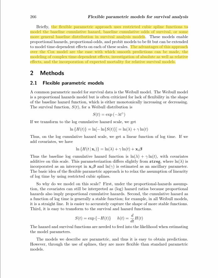
Briefly, the flexible parametric approach uses restricted cubic spline functions tomodel the baseline cumulative hazard, baseline cumulative odds of survival, or somemore general baseline distribution in survival analysis models. These models enableproportional hazards, proportional-odds, and probit models to be fit but can be extendedto model time-dependent effects on each of these scales. The advantages of this approachover the Cox model are the ease with which smooth predictions can be made, themodeling of complex time-dependent effects, investigation of absolute as well as relativeeffects, and the incorporation of expected mortality for relative survival models.

2 Methods

2.1 Flexible parametric models

A common parametric model for survival data is the Weibull model. The Weibull modelis a proportional hazards model but is often criticized for lack of flexibility in the shapeof the baseline hazard function, which is either monotonically increasing or decreasing.The survival function, S(t), for a Weibull distribution is

S(t) = exp (−λtγ)

If we transform to the log cumulative hazard scale, we get

ln {H(t)} = ln[− ln{S(t)}] = ln(λ) + γ ln(t)

Thus, on the log cumulative hazard scale, we get a linear function of log time. If weadd covariates, we have

ln {H(t |xi)} = ln(λ) + γ ln(t) + xiβ

Thus the baseline log cumulative hazard function is ln(λ) + γ ln(t), with covariatesadditive on this scale. This parameterization differs slightly from streg, where ln(λ) isincorporated as an intercept in xiβ and ln(γ) is estimated as an ancillary parameter.The basic idea of the flexible parametric approach is to relax the assumption of linearityof log time by using restricted cubic splines.

So why do we model on this scale? First, under the proportional-hazards assump-tion, the covariates can still be interpreted as (log) hazard ratios because proportionalhazards also imply proportional cumulative hazards. Second, the cumulative hazard asa function of log time is generally a stable function; for example, in all Weibull models,it is a straight line. It is easier to accurately capture the shape of more stable functions.Third, it is easy to transform to the survival and hazard functions.

S(t) = exp {−H(t)} h(t) =d

dtH(t)

The hazard and survival functions are needed to feed into the likelihood when estimatingthe model parameters.

The models we describe are parametric, and thus it is easy to obtain predictions.However, through the use of splines, they are more flexible than standard parametricmodels.

hroth

hroth

P. C. Lambert and P. Royston 267

2.2 Restricted cubic splines

Splines are flexible mathematical functions defined by piecewise polynomials, with someconstraints to ensure that the overall curve is smooth. The points at which the poly-nomials join are called knots. The fitted function is forced to have continuous 0th, 1st,and 2nd derivatives. The most common splines used in practice are cubic splines. Re-gression splines are useful because they can be incorporated into any regression modelwith a linear predictor.

stpm2 uses restricted cubic splines (Durrleman and Simon 1989). These have therestriction that the fitted function is forced to be linear before the first knot and afterthe final knot. Restricted cubic splines with K knots can be fit by creating K−1 derivedvariables. For knots k1, . . . , kK , a restricted cubic spline function can be written as

s(x) = γ0 + γ1z1 + γ2z2 + · · · + γK−1zK−1

The derived variables, zj (also known as the basis functions), are calculated as follows:

z1 = xzj = (x − kj)3+ − φj(x − k1)3+ − (1 − φj)(x − kK)3+ j = 2, . . . , K − 1

where φj = (kK − kj)/(kK − k1).

The derived variables can be highly correlated, and by default, stpm2 orthogonalizesthe derived splines variables by using Gram–Schmidt orthogonalization.

2.3 Flexible parametric models: Incorporating splines

Because the models are on the log cumulative hazard scale, we can write a proportionalhazards model

ln{H(t |xi)} = ln {H0(t)} + xiβ

A restricted cubic spline function of ln(t), with knots k0, can be written ass {ln(t) |γ,k0}. This is then used for the baseline log cumulative hazard in a propor-tional (cumulative) hazards model:

ln{H(t |xi)} = ηi = s {ln(t) |γ,k0} + xiβ (1)

For example, with four knots, we can write

ln {H(t |xi)} = ηi = γ0 + γ1z1i + γ2z2i + γ3z3i + xiβ

We can transform to the survival and hazard scales:

S(t |xi) = exp{− exp(ηi)} h(t |xi) =ds {ln(t) |γ,k0}

dtexp(ηi)

The hazard function involves the derivatives of the restricted cubic splines functions.However, these are easy to calculate:

s′(x) = γ1z′1 + γ2z

′2 + · · · + γK−1z

′K−1


where

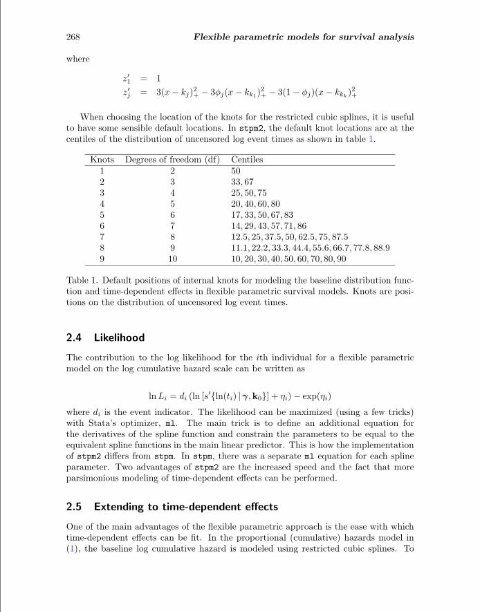
z′1 = 1z′j = 3(x − kj)2+ − 3φj(x − kk1)

2+ − 3(1 − φj)(x − kkk)2+

When choosing the location of the knots for the restricted cubic splines, it is usefulto have some sensible default locations. In stpm2, the default knot locations are at thecentiles of the distribution of uncensored log event times as shown in table 1.

Knots Degrees of freedom (df) Centiles1 2 502 3 33, 673 4 25, 50, 754 5 20, 40, 60, 805 6 17, 33, 50, 67, 836 7 14, 29, 43, 57, 71, 867 8 12.5, 25, 37.5, 50, 62.5, 75, 87.58 9 11.1, 22.2, 33.3, 44.4, 55.6, 66.7, 77.8, 88.99 10 10, 20, 30, 40, 50, 60, 70, 80, 90

Table 1. Default positions of internal knots for modeling the baseline distribution func-tion and time-dependent effects in flexible parametric survival models. Knots are posi-tions on the distribution of uncensored log event times.

2.4 Likelihood

The contribution to the log likelihood for the ith individual for a flexible parametricmodel on the log cumulative hazard scale can be written as

ln Li = di (ln [s′{ln(ti) |γ,k0}] + ηi) − exp(ηi)

where di is the event indicator. The likelihood can be maximized (using a few tricks)with Stata’s optimizer, ml. The main trick is to define an additional equation forthe derivatives of the spline function and constrain the parameters to be equal to theequivalent spline functions in the main linear predictor. This is how the implementationof stpm2 differs from stpm. In stpm, there was a separate ml equation for each splineparameter. Two advantages of stpm2 are the increased speed and the fact that moreparsimonious modeling of time-dependent effects can be performed.

2.5 Extending to time-dependent effects

One of the main advantages of the flexible parametric approach is the ease with whichtime-dependent effects can be fit. In the proportional (cumulative) hazards model in(1), the baseline log cumulative hazard is modeled using restricted cubic splines. To


make effects time dependent, we can just form interactions with the spline terms andthe covariates of interest. In stpm, any time-dependent effects had to have the samenumber of knots at the same locations as the baseline effect. This tended to over-parameterize the time-dependent effects because, generally, the underlying shape of thebaseline hazard is more complex than any departures from it. Thus, in stpm2, time-dependent effects are allowed to have fewer knots and have these knots at differentlocations than for the baseline effect. If there are D time-dependent effects, then wecan write

ln {Hi(t |xi)} = s {ln(t) |γ,k0} +D!

j=1

s {ln(t) | δk,kj}xij + xiβ

The default knot locations for a specified number of degrees of freedom (df) are thesame as those listed for the baseline hazard in table 1. The number of spline variablesfor a particular time-dependent effect will depend on the number of knots, kj . Foreach time-dependent effect, there is an interaction between the covariate and the splinevariables. The model is allowing for nonproportional cumulative hazards, and there willbe a bit of work to convert this to the hazard-ratio scale.

2.6 Hazard ratios

The most common method of summarizing differences between two groups is the hazardratio. When the hazard ratio becomes a function of time, it is generally best to plotit, with 95% confidence intervals, as a function of time. Because the models describedso far are on the (log) cumulative hazard scale and we want to quantify difference onthe (log) hazard scale, we have to perform a nonlinear transformation of the modelparameters.

Consider a model with one dichotomous covariate, x1, taking on the values 1 and0 and that has a time-dependent effect. The log hazard-ratio comparing x1 = 1 withx1 = 0 at time t0 can be written as

ln(HR) = ln [s′ {ln(t0) |γ,k0} + s′ {ln(t0) | δ1,k1}] − ln [s′ {ln(t0) | δ1,k1}]+ s {ln(t0) | δ1,k1} + β1

Because this is a nonlinear function of the parameters, the standard error (and thusthe confidence interval) of the log hazard-ratio at time t0 is obtained with the deltamethod by using the Stata predictnl command, where the derivatives are calculatednumerically. This is a further enhancement over stpm.

2.7 Other predictions

stpm2 also enables other useful predictions for quantifying differences between groups.The first of these is the difference in hazard rates between any two covariate patterns.The second is the difference in survival curves between any two covariate patterns.


Confidence intervals are obtained by applying the delta method by using predictnl.It is also possible to calculate and compare centiles of the survival distribution. Thisinvolves an iterative process using the Newton–Raphson algorithm.

2.8 Delayed entry

stpm2, like most Stata st commands, can incorporate delayed entry. This means thatsome subjects become at risk at some time after time t = 0. This is also known as left-truncation. A common example in epidemiology is when age is used as the time scale,so subjects become at risk at the age they were diagnosed with the disease under study(Cheung, Gao, and Khoo 2003). A further example, used in relative survival models,is when using period analysis where up-to-date estimates of survival are obtained byartificially left-truncating the time scale so that only the most recent data are usedto estimate survival (Brenner and Gefeller 1997). Delayed entry is also needed whenincorporating time-dependent covariates or piecewise time-dependent effects similarlyto the Cox model (Cleves et al. 2008).

2.9 Modeling on other scales

Royston and Parmar (2002) discuss the use of models on other scales. These includeflexible proportional-odds models, probit models, and a more general model that involvestransformation of the survival function based on a suggestion by Aranda-Ordaz (1981).All these models are available in stpm2.

2.10 Relative survival

Relative survival is a common method used in population-based cancer studies. Inthese studies, mortality associated with the cancer under study is of the most interest.However, cause of death information is often not available or is otherwise considered tobe unreliable. Therefore, mortality associated with the disease of interest is estimatedby incorporating expected (or background) mortality, which can usually be obtainedfrom national or regional life tables. In relative survival, the all-cause survival function,S(t), can be expressed as the product of the expected survival function, S∗(t), and therelative survival function, R(t):

S(t) = S∗(t)R(t)

Transforming to the hazard scale gives

h(t) = h∗(t) + λd(t)

where h(t) is the all-cause hazard (mortality) rate, h∗(t) is the expected hazard (mor-tality) rate, and λd(t) is the excess hazard (mortality) rate associated with the diseaseof interest. Thus the mortality rate is the sum of two components: the backgroundmortality rate and the excess mortality rate associated with the disease. The flexible


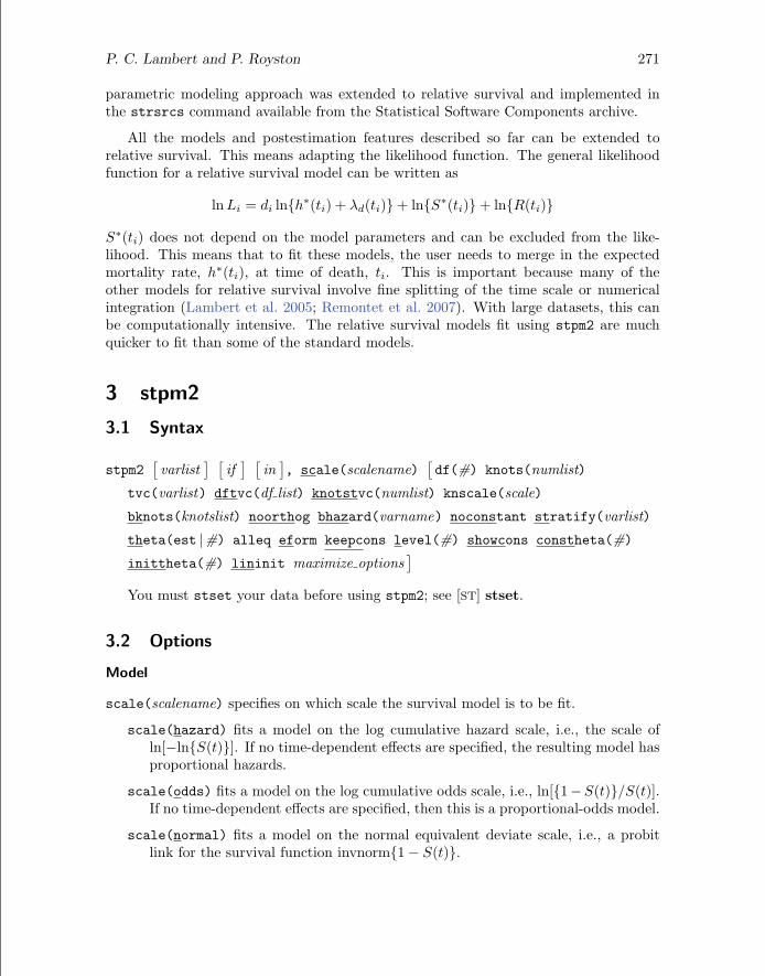
parametric modeling approach was extended to relative survival and implemented inthe strsrcs command available from the Statistical Software Components archive.

All the models and postestimation features described so far can be extended torelative survival. This means adapting the likelihood function. The general likelihoodfunction for a relative survival model can be written as

ln Li = di ln{h∗(ti) + λd(ti)} + ln{S∗(ti)} + ln{R(ti)}

S∗(ti) does not depend on the model parameters and can be excluded from the like-lihood. This means that to fit these models, the user needs to merge in the expectedmortality rate, h∗(ti), at time of death, ti. This is important because many of theother models for relative survival involve fine splitting of the time scale or numericalintegration (Lambert et al. 2005; Remontet et al. 2007). With large datasets, this canbe computationally intensive. The relative survival models fit using stpm2 are muchquicker to fit than some of the standard models.

3 stpm2

3.1 Syntax

stpm2"varlist

# "if

# "in

#, scale(scalename)

"df(#) knots(numlist)

tvc(varlist) dftvc(df list) knotstvc(numlist) knscale(scale)bknots(knotslist) noorthog bhazard(varname) noconstant stratify(varlist)theta(est |#) alleq eform keepcons level(#) showcons constheta(#)

inittheta(#) lininit maximize options#

You must stset your data before using stpm2; see [ST] stset.

3.2 Options

Model

scale(scalename) specifies on which scale the survival model is to be fit.

scale(hazard) fits a model on the log cumulative hazard scale, i.e., the scale ofln[−ln{S(t)}]. If no time-dependent effects are specified, the resulting model hasproportional hazards.

scale(odds) fits a model on the log cumulative odds scale, i.e., ln[{1−S(t)}/S(t)].If no time-dependent effects are specified, then this is a proportional-odds model.

scale(normal) fits a model on the normal equivalent deviate scale, i.e., a probitlink for the survival function invnorm{1 − S(t)}.


scale(theta) fits a model on a scale defined by the value of θ for the Aranda-Ordaz family of link functions, i.e., ln[{S(t)(−θ) − 1}/θ]. θ = 1 corresponds to aproportional-odds model, and θ = 0 corresponds to a proportional cumulative-hazard model.

df(#) specifies the df for the restricted cubic spline function used for the baselinehazard rate. # must be between 1 and 10, but a value between 1 and 5 is usuallysufficient. The knots are placed at the centiles of the distribution of the uncensoredlog times as shown in table 1. Using df(1) is equivalent to fitting a Weibull modelwhen using scale(hazard).

knots(numlist) specifies knot locations for the baseline distribution function, as op-posed to the default locations set by df(). The locations of the knots are placedon the scale defined by knscale(). However, the scale used by the restricted cubicspline function is always log time. Default knot positions are determined by thedf() option.

tvc(varlist) specifies the names of the variables that are time dependent. Time-dependent effects are fit using restricted cubic splines. The df is specified usingthe dftvc() option.

dftvc(df list) specifies the df for time-dependent effects. The potential df is between 1and 10. With 1 degree of freedom, a linear effect of log time is fit. If there is morethan one time-dependent effect and a different df is required for each time-dependenteffect, then the following syntax can be used: dftvc(x1:3 x2:2 1), where x1 has3 df, x2 has 2 df, and any remaining time-dependent effects have 1 df.

knotstvc(numlist) specifies the location of the internal knots for any time-dependenteffects. If different knots are required for different time-dependent effects, then thisoption can be specified as follows: knotstvc(x1 1 2 3 x2 1.5 3.5).

knscale(scale) sets the scale on which user-defined knots are specified. knscale(time)denotes the original time scale, knscale(log) denotes the log time scale, andknscale(centile) specifies that the knots are taken to be centile positions in thedistribution of the uncensored log survival times. The default is knscale(time).

bknots(knotslist) is a two-element list giving the boundary knots. By default, theseare located at the minimum and maximum of the uncensored survival times. Theyare specified on the scale defined by knscale().

noorthog suppresses orthogonal transformation of spline variables.

bhazard(varname) is used when fitting relative survival models. varname gives theexpected mortality rate at the time of death or censoring. stpm2 gives an errormessage when there are missing values of varname, because this usually indicatesthat an error has occurred when merging the expected mortality rates.

noconstant; see [R] estimation options.


stratify(varlist) is provided for backward compatibility with stpm. Members of varlistare modeled with time-dependent effects. See the tvc() and dftvc() options forstpm2’s way of specifying time-dependent effects.

theta(est |#) is provided for backward compatibility with stpm. est requests thatθ be estimated, whereas # fixes θ to #. See constheta() and inittheta() forstpm2’s way of specifying θ.

Reporting

alleq reports all equations used by ml. The models are fit using various constraints forparameters associated with the derivatives of the spline functions. These parametersare generally not of interest and thus are not shown by default. Also, an extraequation is used when fitting delayed-entry models; again, this is not shown bydefault.

eform reports the exponentiated coefficients. For models on the log cumulative-hazardscale, scale(hazard), this gives hazard ratios if the covariate is not time dependent.Similarly, for models on the log cumulative-odds scale, scale(odds), this option willgive odds ratios for non–time-dependent effects.

keepcons prevents the constraints imposed by stpm2 on the derivatives of the splinefunction when fitting delayed-entry models from being dropped. By default, theconstraints are dropped.

level(#) specifies the confidence level, as a percentage, for confidence intervals. Thedefault is level(95) or as set by set level.

showcons lists in the output the constraints used by stpm2 for the derivatives of thespline function and when fitting delayed-entry models; the default is to not list them.

Max options

constheta(#) constrains the value of θ; i.e., it is treated as a known constant.

inittheta(#) specifies an initial value for θ in the Aranda-Ordaz family of link func-tions.

lininit obtains initial values by fitting only the first spline basis function (i.e., a linearfunction of log survival time). This option is seldom needed.

maximize options: difficult, technique(algorithm spec), iterate(#),"no

#log,

trace, gradient, showstep, hessian, shownrtolerance, tolerance(#),ltolerance(#), gtolerance(#), nrtolerance(#), nonrtolerance,from(init specs); see [R] maximize. These options are seldom used, but difficultmay be useful if there are convergence problems when fitting models that use theAranda-Ordaz family of link functions.


4 stpm2 postestimation

stpm2 is an estimation command and thus shares most of the features of Stata estima-tion commands; see [U] 20 Estimation and postestimation commands. The rangeof predictions available postestimation when using stpm2 has been much extended com-pared with the range available for stpm. The predictions available are briefly describedbelow.

4.1 Syntax

predict newvar"if

# "in

# ", at(varname #

"varname # . . .

#)

centile(# | varname) ci cumhazard cumodds density hazard

hdiff1(varname #"varname # . . .

#) hdiff2(varname #

"varname #

. . .#) hrdenominator(varname #

"varname # . . .

#) hrnumerator(varname

#"varname # . . .

#) martingale meansurv normal sdiff1(varname #

"varname # . . .

#) sdiff2(varname #

"varname # . . .

#) stdp survival

timevar(varname) xb xbnobaseline zeros centol(#) deviance dxb

level(#)#

4.2 Options

Main

at(varname #"varname # . . .

#) requests that the covariates specified by varname

be set to #. This is a useful way to obtain out-of-sample predictions. If at() is usedtogether with zeros, then all covariates not listed in at() are set to zero. If at()is used without zeros, then all covariates not listed in at() are set to their samplevalues.

centile(# | varname) requests the #th centile of survival-time distribution, calculatedusing the Newton–Raphson algorithm (or requests the centiles stored in varname).

ci calculates a confidence interval for the requested statistic and stores the confidencelimits in newvar lci and newvar uci.

cumhazard predicts the cumulative hazard function.

cumodds predicts the cumulative odds-of-failure function.

density predicts the density function.

hazard predicts the hazard rate (or excess hazard rate if stpm2’s bhazard() option wasused).


hdiff1(varname #"varname # . . .

#) and hdiff2(varname #

"varname # . . .

#)

predict the difference in hazard functions, with the first hazard function defined bythe covariate values listed for hdiff1() and the second, by those listed for hdiff2().By default, covariates not specified using either option are set to zero. Setting theremaining values of the covariates to zero may not always be sensible. If # is set tomissing (.), then varname has the values defined in the dataset.

Example: hdiff1(hormon 1) (without specifying hdiff2()) computes the differ-ence in predicted hazard functions at hormon = 1 compared with hormon = 0.

Example: hdiff1(hormon 2) hdiff2(hormon 1) computes the difference in pre-dicted hazard functions at hormon = 2 compared with hormon = 1.

Example: hdiff1(hormon 2 age 50) hdiff2(hormon 1 age 30) computes thedifference in predicted hazard functions at hormon = 2 and age = 50 comparedwith hormon = 1 and age = 30.

hrdenominator(varname #"varname # . . .

#) specifies the denominator of the haz-

ard ratio. By default, all covariates not specified using this option are set to zero.See the cautionary note in hrnumerator() below. If # is set to missing (.), thenthe covariate has the values defined in the dataset.

hrnumerator(varname #"varname # . . .

#) specifies the numerator of the (time-

dependent) hazard ratio. By default, all covariates not specified using this optionare set to zero. Setting the remaining values of the covariates to zero may not alwaysbe sensible, particularly on models other than those on the cumulative hazard scaleor when more than one variable has a time-dependent effect. If # is set to missing(.), then the covariate has the values defined in the dataset.

martingale calculates martingale residuals.

meansurv calculates the population-averaged survival curve. This differs from the pre-dicted survival curve at the mean of all the covariates in the model. A predictedsurvival curve is obtained for each subject, and all the survival curves in a popula-tion are averaged. The process can be computationally intensive. It is recommendedthat the timevar() option be used to reduce the number of survival times at whichthe survival curves are averaged. Combining meansurv with the at() option enablesadjusted survival curves to be estimated.

normal predicts the standard normal deviate of the survival function.

sdiff1(varname #"varname # . . .

#) and sdiff2(varname #

"varname # . . .

#)

predict the difference in survival curves, with the first survival curve defined by thecovariate values listed for sdiff1() and the second, by those listed for sdiff2().By default, covariates not specified using either option are set to zero. Setting theremaining values of the covariates to zero may not always be sensible. If # is set tomissing (.), then varname has the values defined in the dataset.

Example: sdiff1(hormon 1) (without specifying sdiff2()) computes the differ-ence in predicted survival curves at hormon = 1 compared with hormon = 0.


Example: sdiff1(hormon 2) sdiff2(hormon 1) computes the difference in pre-dicted survival curves at hormon = 2 compared with hormon = 1.

Example: sdiff1(hormon 2 age 50) sdiff2(hormon 1 age 30) computes thedifference in predicted survival curves at hormon = 2 and age = 50 compared withhormon = 1 and age = 30.

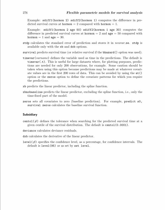
stdp calculates the standard error of prediction and stores it in newvar se. stdp isavailable only with the xb and dxb options.

survival predicts survival time (or relative survival if the bhazard() option was used).

timevar(varname) defines the variable used as time in the predictions. The default istimevar( t). This is useful for large datasets where, for plotting purposes, predic-tions are needed for only 200 observations, for example. Some caution should betaken when using this option because predictions may be made at whatever covari-ate values are in the first 200 rows of data. This can be avoided by using the at()option or the zeros option to define the covariate patterns for which you requirethe predictions.

xb predicts the linear predictor, including the spline function.

xbnobaseline predicts the linear predictor, excluding the spline function, i.e., only thetime-fixed part of the model.

zeros sets all covariates to zero (baseline prediction). For example, predict s0,survival zeros calculates the baseline survival function.

Subsidiary

centol(#) defines the tolerance when searching for the predicted survival time at agiven centile of the survival distribution. The default is centol(0.0001).

deviance calculates deviance residuals.

dxb calculates the derivative of the linear predictor.

level(#) specifies the confidence level, as a percentage, for confidence intervals. Thedefault is level(95) or as set by set level.


5 Examples

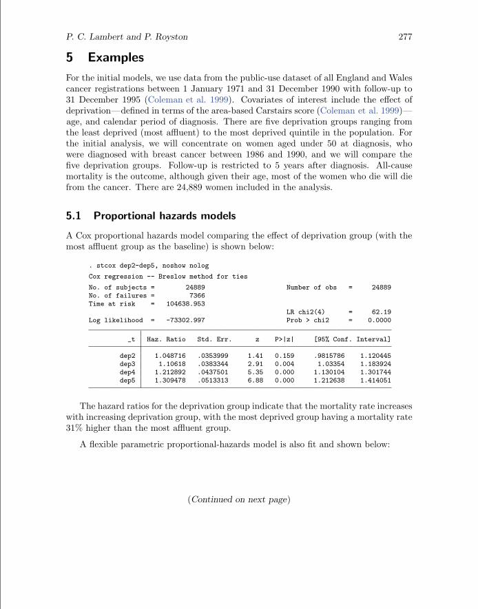
For the initial models, we use data from the public-use dataset of all England and Walescancer registrations between 1 January 1971 and 31 December 1990 with follow-up to31 December 1995 (Coleman et al. 1999). Covariates of interest include the effect ofdeprivation—defined in terms of the area-based Carstairs score (Coleman et al. 1999)—age, and calendar period of diagnosis. There are five deprivation groups ranging fromthe least deprived (most affluent) to the most deprived quintile in the population. Forthe initial analysis, we will concentrate on women aged under 50 at diagnosis, whowere diagnosed with breast cancer between 1986 and 1990, and we will compare thefive deprivation groups. Follow-up is restricted to 5 years after diagnosis. All-causemortality is the outcome, although given their age, most of the women who die will diefrom the cancer. There are 24,889 women included in the analysis.

5.1 Proportional hazards models

A Cox proportional hazards model comparing the effect of deprivation group (with themost affluent group as the baseline) is shown below:

. stcox dep2-dep5, noshow nolog

Cox regression -- Breslow method for ties

No. of subjects = 24889 Number of obs = 24889No. of failures = 7366Time at risk = 104638.953

LR chi2(4) = 62.19Log likelihood = -73302.997 Prob > chi2 = 0.0000

_t Haz. Ratio Std. Err. z P>|z| [95% Conf. Interval]

dep2 1.048716 .0353999 1.41 0.159 .9815786 1.120445dep3 1.10618 .0383344 2.91 0.004 1.03354 1.183924dep4 1.212892 .0437501 5.35 0.000 1.130104 1.301744dep5 1.309478 .0513313 6.88 0.000 1.212638 1.414051

The hazard ratios for the deprivation group indicate that the mortality rate increaseswith increasing deprivation group, with the most deprived group having a mortality rate31% higher than the most affluent group.

A flexible parametric proportional-hazards model is also fit and shown below:

(Continued on next page)


. stpm2 dep2-dep5, df(5) scale(hazard) eform nolog

Log likelihood = -22502.633 Number of obs = 24889

exp(b) Std. Err. z P>|z| [95% Conf. Interval]

xbdep2 1.048752 .0354011 1.41 0.158 .9816125 1.120483dep3 1.10615 .0383334 2.91 0.004 1.033513 1.183893dep4 1.212872 .0437493 5.35 0.000 1.130085 1.301722dep5 1.309479 .0513313 6.88 0.000 1.212639 1.414052_rcs1 2.126897 .0203615 78.83 0.000 2.087361 2.167182_rcs2 .9812977 .0074041 -2.50 0.012 .9668927 .9959173_rcs3 1.057255 .0043746 13.46 0.000 1.048715 1.065863_rcs4 1.005372 .0020877 2.58 0.010 1.001288 1.009472_rcs5 1.002216 .0010203 2.17 0.030 1.000218 1.004218

The df(5) option implies using 5 df (4 internal knots) at their default locations. Thescale(hazard) option states that the model is being fit on the log cumulative hazardscale. The estimated hazard ratios and their 95% confidence intervals are very similarto the Cox model, and in fact, there is no difference up to four decimal places. We haveyet to find an example of a proportional hazards model where there is a large differencein the estimated hazard ratios between these two models.

The advantage of using the parametric approach is the ease of obtaining predictions.The following code obtains the predictions for the linear predictor, the survival function,and the hazard function. Confidence intervals can be obtained by adding the ci option.


predict xb, xbpredict s, survivalpredict h, hazard

−8

−6

−4

−2

0

log

cum

ulat

ive h

azar

d

0 1 2 3 4 5Time from Diagnosis (years)

(a)

−8

−6

−4

−2

0

log

cum

ulat

ive h

azar

d

1 2 3 45Time from Diagnosis (years)

(b)

.6

.7

.8

.9

1

Surv

ival


(c)

0255075

100125150

Mor

tality

Rat

e (p

er 1

000

py)


(d)

Least Deprived 2 3 4 Most DeprivedDeprivation Group

Figure 1. Predictions from proportional hazards model for breast cancer data

Figure 1(a) shows the predicted log cumulative hazard function. This is the scale weare modeling on. Figure 1(b) also shows the predicted log cumulative hazard function,but now it is plotted against log time. This shows the reason why the splines are afunction of log time; the curve is generally much more stable on this scale. Figure 1(c)shows the predicted survival curves for the five deprivation groups. This shows thatsurvival is worse as deprivation increases. Finally, figure 1(d) shows the predicted hazardfunction. The hazard function has been multiplied by 1,000 to give the mortality rateper 1,000 person-years. There is an initial sharp decrease in the hazard rate, followed byan increase until about 1.5 years. Because these fitted values come from a proportionalhazards model, these lines are all proportional.

5.2 Time-dependent effects

One option to fit time-dependent hazard ratios is to use stsplit to split the time scaleand fit piecewise hazard ratios. See Cleves et al. (2008) for examples of how to do thisfor a Cox model. However, we will concentrate on continuous time-dependent effectsusing restricted cubic splines.

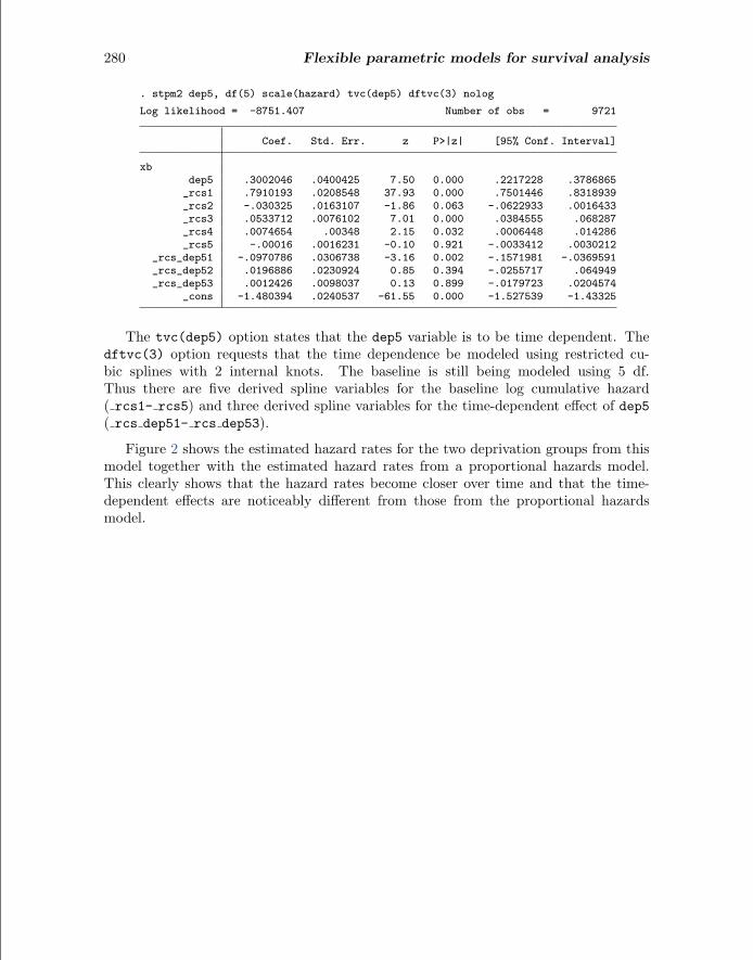
For simplicity, we have dropped the three middle deprivation groups and are justcomparing the most deprived group with the most affluent group. The following codeallows the effect of deprivation group 5 (dep5) to be time dependent:


. stpm2 dep5, df(5) scale(hazard) tvc(dep5) dftvc(3) nolog


Coef. Std. Err. z P>|z| [95% Conf. Interval]

xbdep5 .3002046 .0400425 7.50 0.000 .2217228 .3786865_rcs1 .7910193 .0208548 37.93 0.000 .7501446 .8318939_rcs2 -.030325 .0163107 -1.86 0.063 -.0622933 .0016433_rcs3 .0533712 .0076102 7.01 0.000 .0384555 .068287_rcs4 .0074654 .00348 2.15 0.032 .0006448 .014286_rcs5 -.00016 .0016231 -0.10 0.921 -.0033412 .0030212

_rcs_dep51 -.0970786 .0306738 -3.16 0.002 -.1571981 -.0369591_rcs_dep52 .0196886 .0230924 0.85 0.394 -.0255717 .064949_rcs_dep53 .0012426 .0098037 0.13 0.899 -.0179723 .0204574

_cons -1.480394 .0240537 -61.55 0.000 -1.527539 -1.43325

The tvc(dep5) option states that the dep5 variable is to be time dependent. Thedftvc(3) option requests that the time dependence be modeled using restricted cu-bic splines with 2 internal knots. The baseline is still being modeled using 5 df.Thus there are five derived spline variables for the baseline log cumulative hazard( rcs1- rcs5) and three derived spline variables for the time-dependent effect of dep5( rcs dep51- rcs dep53).

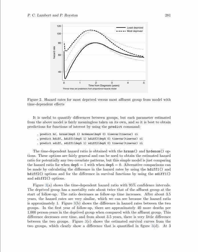
Figure 2 shows the estimated hazard rates for the two deprivation groups from thismodel together with the estimated hazard rates from a proportional hazards model.This clearly shows that the hazard rates become closer over time and that the time-dependent effects are noticeably different from those from the proportional hazardsmodel.


40

60

80

100

120

haza

rd ra

te


Least deprivedMost deprived

Thinner lines are predictions from proportional hazards model

Figure 2. Hazard rates for most deprived versus most affluent group from model withtime-dependent effects

It is useful to quantify differences between groups, but each parameter estimatedfrom the above model is fairly meaningless taken on its own, and so it is best to obtainpredictions for functions of interest by using the predict command:

. predict hr, hrnum(dep5 1) hrdenom(dep5 0) timevar(timevar) ci

. predict hdiff, hdiff1(dep5 1) hdiff2(dep5 0) timevar(timevar) ci

. predict sdiff, sdiff1(dep5 1) sdiff2(dep5 0) timevar(timevar) ci

The time-dependent hazard ratio is obtained with the hrnum() and hrdenom() op-tions. These options are fairly general and can be used to obtain the estimated hazardratio for potentially any two covariate patterns, but this simple model is just comparingthe hazard ratio for when dep5 = 1 with when dep5 = 0. Alternative comparisons canbe made by calculating the difference in the hazard rates by using the hdiff1() andhdiff2() options and for the difference in survival functions by using the sdiff1()and sdiff2() options.

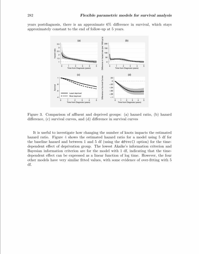
Figure 3(a) shows the time-dependent hazard ratio with 95% confidence intervals.The deprived group has a mortality rate about twice that of the affluent group at thestart of follow-up. The ratio decreases as follow-up time increases. After about 3.5years, the hazard rates are very similar, which we can see because the hazard ratiois approximately 1. Figure 3(b) shows the difference in hazard rates between the twogroups. In the first year of follow-up, there are approximately 40 more deaths per1,000 person-years in the deprived group when compared with the affluent group. Thisdifference decreases over time, and from about 3.5 years, there is very little differencebetween the two groups. Figure 3(c) shows the estimated survival curves from thetwo groups, which clearly show a difference that is quantified in figure 3(d). At 3


years postdiagnosis, there is an approximate 6% difference in survival, which staysapproximately constant to the end of follow-up at 5 years.

1

1.5

2

2.5

3

3.5

haza

rd ra

tio


(a)

0

50

100

150

200

Diffe

renc

e in

haz

ard

rate

(per

100

0 py

’s)


(b)

.4

.6

.8

1

Surv

ival


Least deprivedMost deprived

(c)

−.1−.08−.06−.04−.02

0.02

Diffe

renc

e in

Sur

vival

Cur

ves


(d)

Figure 3. Comparison of affluent and deprived groups: (a) hazard ratio, (b) hazarddifference, (c) survival curves, and (d) difference in survival curves

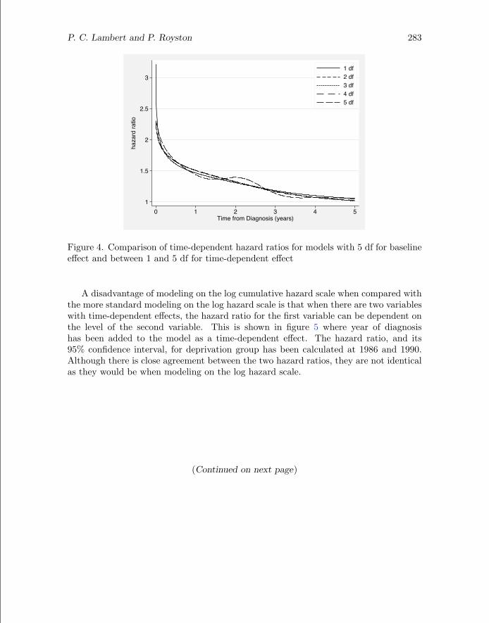
It is useful to investigate how changing the number of knots impacts the estimatedhazard ratio. Figure 4 shows the estimated hazard ratio for a model using 5 df forthe baseline hazard and between 1 and 5 df (using the dftvc() option) for the time-dependent effect of deprivation group. The lowest Akaike’s information criterion andBayesian information criterion are for the model with 1 df, indicating that the time-dependent effect can be expressed as a linear function of log time. However, the fourother models have very similar fitted values, with some evidence of over-fitting with 5df.


1

1.5

2

2.5

3

haza

rd ra

tio


1 df2 df3 df4 df5 df

Figure 4. Comparison of time-dependent hazard ratios for models with 5 df for baselineeffect and between 1 and 5 df for time-dependent effect

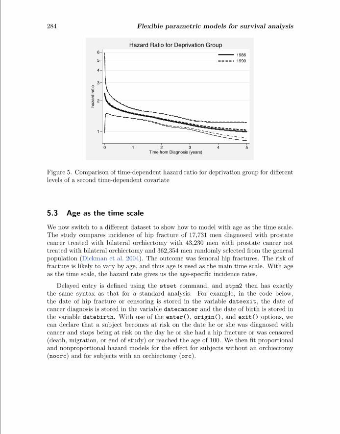
A disadvantage of modeling on the log cumulative hazard scale when compared withthe more standard modeling on the log hazard scale is that when there are two variableswith time-dependent effects, the hazard ratio for the first variable can be dependent onthe level of the second variable. This is shown in figure 5 where year of diagnosishas been added to the model as a time-dependent effect. The hazard ratio, and its95% confidence interval, for deprivation group has been calculated at 1986 and 1990.Although there is close agreement between the two hazard ratios, they are not identicalas they would be when modeling on the log hazard scale.



1

2

3

4

5

6

haza

rd ra

tio


19861990

Hazard Ratio for Deprivation Group

Figure 5. Comparison of time-dependent hazard ratio for deprivation group for differentlevels of a second time-dependent covariate

5.3 Age as the time scale

We now switch to a different dataset to show how to model with age as the time scale.The study compares incidence of hip fracture of 17,731 men diagnosed with prostatecancer treated with bilateral orchiectomy with 43,230 men with prostate cancer nottreated with bilateral orchiectomy and 362,354 men randomly selected from the generalpopulation (Dickman et al. 2004). The outcome was femoral hip fractures. The risk offracture is likely to vary by age, and thus age is used as the main time scale. With ageas the time scale, the hazard rate gives us the age-specific incidence rates.

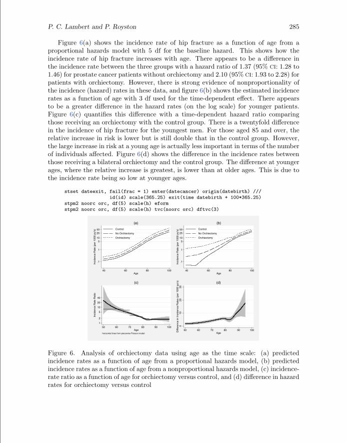
Delayed entry is defined using the stset command, and stpm2 then has exactlythe same syntax as that for a standard analysis. For example, in the code below,the date of hip fracture or censoring is stored in the variable dateexit, the date ofcancer diagnosis is stored in the variable datecancer and the date of birth is stored inthe variable datebirth. With use of the enter(), origin(), and exit() options, wecan declare that a subject becomes at risk on the date he or she was diagnosed withcancer and stops being at risk on the day he or she had a hip fracture or was censored(death, migration, or end of study) or reached the age of 100. We then fit proportionaland nonproportional hazard models for the effect for subjects without an orchiectomy(noorc) and for subjects with an orchiectomy (orc).


Figure 6(a) shows the incidence rate of hip fracture as a function of age from aproportional hazards model with 5 df for the baseline hazard. This shows how theincidence rate of hip fracture increases with age. There appears to be a difference inthe incidence rate between the three groups with a hazard ratio of 1.37 (95% CI: 1.28 to1.46) for prostate cancer patients without orchiectomy and 2.10 (95% CI: 1.93 to 2.28) forpatients with orchiectomy. However, there is strong evidence of nonproportionality ofthe incidence (hazard) rates in these data, and figure 6(b) shows the estimated incidencerates as a function of age with 3 df used for the time-dependent effect. There appearsto be a greater difference in the hazard rates (on the log scale) for younger patients.Figure 6(c) quantifies this difference with a time-dependent hazard ratio comparingthose receiving an orchiectomy with the control group. There is a twentyfold differencein the incidence of hip fracture for the youngest men. For those aged 85 and over, therelative increase in risk is lower but is still double that in the control group. However,the large increase in risk at a young age is actually less important in terms of the numberof individuals affected. Figure 6(d) shows the difference in the incidence rates betweenthose receiving a bilateral orchiectomy and the control group. The difference at youngerages, where the relative increase is greatest, is lower than at older ages. This is due tothe incidence rate being so low at younger ages.

stset dateexit, fail(frac = 1) enter(datecancer) origin(datebirth) ///id(id) scale(365.25) exit(time datebirth + 100*365.25)

stpm2 noorc orc, df(5) scale(h) eformstpm2 noorc orc, df(5) scale(h) tvc(noorc orc) dftvc(3)

.1

1

5102550

Incid

ence

Rat

e (p

er 1

000

py’s)

40 60 80 100Age

ControlNo OrchiectomyOrchiectomy

(a)

.1

1

5102550

Incid

ence

Rat

e (p

er 1

000

py’s)

40 60 80 100Age

ControlNo OrchiectomyOrchiectomy

(b)

12

5102040

Incid

ence

Rat

e Ra

tio

50 60 70 80 90 100Age

horizontal lines from piecewise Poisson model

(c)

010

2030

Diffe

renc

e in

Incid

ence

Rat

es (p

er 1

000

py’s)

50 60 70 80 90 100Age

(d)

Figure 6. Analysis of orchiectomy data using age as the time scale: (a) predictedincidence rates as a function of age from a proportional hazards model, (b) predictedincidence rates as a function of age from a nonproportional hazards model, (c) incidence-rate ratio as a function of age for orchiectomy versus control, and (d) difference in hazardrates for orchiectomy versus control


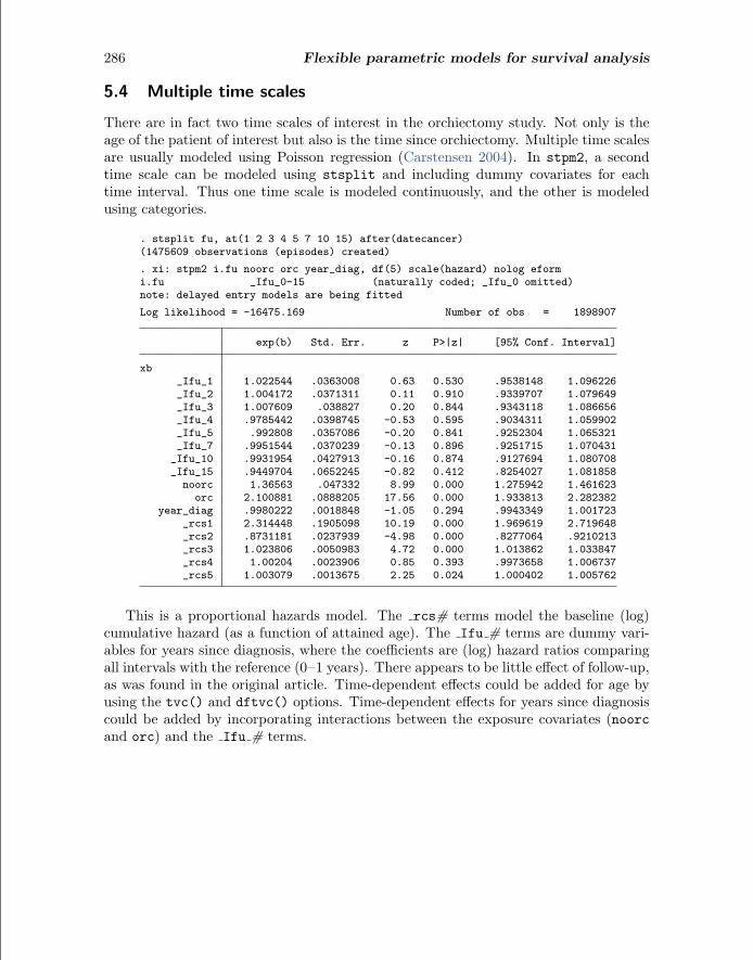
5.4 Multiple time scales

There are in fact two time scales of interest in the orchiectomy study. Not only is theage of the patient of interest but also is the time since orchiectomy. Multiple time scalesare usually modeled using Poisson regression (Carstensen 2004). In stpm2, a secondtime scale can be modeled using stsplit and including dummy covariates for eachtime interval. Thus one time scale is modeled continuously, and the other is modeledusing categories.

. stsplit fu, at(1 2 3 4 5 7 10 15) after(datecancer)(1475609 observations (episodes) created)

. xi: stpm2 i.fu noorc orc year_diag, df(5) scale(hazard) nolog eformi.fu _Ifu_0-15 (naturally coded; _Ifu_0 omitted)note: delayed entry models are being fitted



xb_Ifu_1 1.022544 .0363008 0.63 0.530 .9538148 1.096226_Ifu_2 1.004172 .0371311 0.11 0.910 .9339707 1.079649_Ifu_3 1.007609 .038827 0.20 0.844 .9343118 1.086656_Ifu_4 .9785442 .0398745 -0.53 0.595 .9034311 1.059902_Ifu_5 .992808 .0357086 -0.20 0.841 .9252304 1.065321_Ifu_7 .9951544 .0370239 -0.13 0.896 .9251715 1.070431_Ifu_10 .9931954 .0427913 -0.16 0.874 .9127694 1.080708_Ifu_15 .9449704 .0652245 -0.82 0.412 .8254027 1.081858

noorc 1.36563 .047332 8.99 0.000 1.275942 1.461623orc 2.100881 .0888205 17.56 0.000 1.933813 2.282382

year_diag .9980222 .0018848 -1.05 0.294 .9943349 1.001723_rcs1 2.314448 .1905098 10.19 0.000 1.969619 2.719648_rcs2 .8731181 .0237939 -4.98 0.000 .8277064 .9210213_rcs3 1.023806 .0050983 4.72 0.000 1.013862 1.033847_rcs4 1.00204 .0023906 0.85 0.393 .9973658 1.006737_rcs5 1.003079 .0013675 2.25 0.024 1.000402 1.005762

This is a proportional hazards model. The rcs# terms model the baseline (log)cumulative hazard (as a function of attained age). The Ifu # terms are dummy vari-ables for years since diagnosis, where the coefficients are (log) hazard ratios comparingall intervals with the reference (0–1 years). There appears to be little effect of follow-up,as was found in the original article. Time-dependent effects could be added for age byusing the tvc() and dftvc() options. Time-dependent effects for years since diagnosiscould be added by incorporating interactions between the exposure covariates (noorcand orc) and the Ifu # terms.


5.5 Relative survival

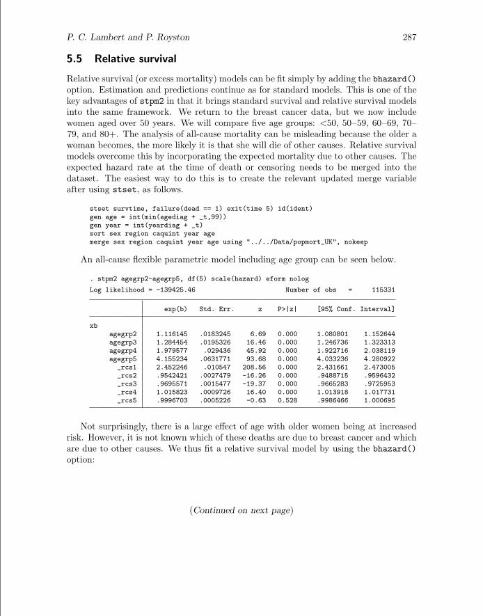
Relative survival (or excess mortality) models can be fit simply by adding the bhazard()option. Estimation and predictions continue as for standard models. This is one of thekey advantages of stpm2 in that it brings standard survival and relative survival modelsinto the same framework. We return to the breast cancer data, but we now includewomen aged over 50 years. We will compare five age groups: <50, 50–59, 60–69, 70–79, and 80+. The analysis of all-cause mortality can be misleading because the older awoman becomes, the more likely it is that she will die of other causes. Relative survivalmodels overcome this by incorporating the expected mortality due to other causes. Theexpected hazard rate at the time of death or censoring needs to be merged into thedataset. The easiest way to do this is to create the relevant updated merge variableafter using stset, as follows.

stset survtime, failure(dead == 1) exit(time 5) id(ident)gen age = int(min(agediag + _t,99))gen year = int(yeardiag + _t)sort sex region caquint year agemerge sex region caquint year age using "../../Data/popmort_UK", nokeep

An all-cause flexible parametric model including age group can be seen below.

. stpm2 agegrp2-agegrp5, df(5) scale(hazard) eform nolog



xbagegrp2 1.116145 .0183245 6.69 0.000 1.080801 1.152644agegrp3 1.284454 .0195326 16.46 0.000 1.246736 1.323313agegrp4 1.979577 .029436 45.92 0.000 1.922716 2.038119agegrp5 4.155234 .0631771 93.68 0.000 4.033236 4.280922

_rcs1 2.452246 .010547 208.56 0.000 2.431661 2.473005_rcs2 .9542421 .0027479 -16.26 0.000 .9488715 .9596432_rcs3 .9695571 .0015477 -19.37 0.000 .9665283 .9725953_rcs4 1.015823 .0009726 16.40 0.000 1.013918 1.017731_rcs5 .9996703 .0005226 -0.63 0.528 .9986466 1.000695

Not surprisingly, there is a large effect of age with older women being at increasedrisk. However, it is not known which of these deaths are due to breast cancer and whichare due to other causes. We thus fit a relative survival model by using the bhazard()option:



. stpm2 agegrp2-agegrp5, df(5) scale(hazard) bhazard(rate) eform nolog

Number of obs = 115331Wald chi2(4) = 3267.44

Log likelihood = -133915.41 Prob > chi2 = 0.0000


xbagegrp2 1.051428 .0182859 2.88 0.004 1.016192 1.087886agegrp3 1.072864 .0181672 4.15 0.000 1.037842 1.109069agegrp4 1.411935 .0250603 19.44 0.000 1.363662 1.461917agegrp5 2.651379 .0510765 50.62 0.000 2.553137 2.753401

_rcs1 2.342038 .0111471 178.80 0.000 2.320292 2.363988_rcs2 .9607407 .0030349 -12.68 0.000 .9548108 .9667075_rcs3 .9697656 .0017879 -16.65 0.000 .9662677 .9732762_rcs4 1.022492 .0011734 19.38 0.000 1.020195 1.024794_rcs5 1.000382 .0006277 0.61 0.543 .9991522 1.001613

In a relative survival model, we get excess hazard ratios as opposed to hazard ratios.The excess hazard ratios are lower than the hazard ratios because the latter incorporatemortality due to both breast cancer and mortality due to other causes.

All the topics covered so far are easily extended to relative survival. Thus we canfit models with smooth estimates of the baseline excess hazard. We can estimate ex-cess hazard ratios and time-dependent excess hazard ratios. We can model on theproportional-odds and other scales. We can use age as the time scale. We can usemultiple time scales. We can easily obtain predictions of the baseline excess hazard,relative survival, time-dependent excess hazard ratios, difference in excess hazard rates,etc.

One useful summary is to report centiles of the survival function. The table belowshows the time at which the relative survival function = 0.75, i.e., an estimate of thetime at which 25% of women have died of breast cancer, with 95% confidence intervals.

. tabdisp agegrp, cellvar(c25 c25_lci c25_uci) format(%4.2f)

agegrp c25 c25_lci c25_uci

1 3.94 3.83 4.052 3.41 3.31 3.513 2.89 2.81 2.974 1.75 1.70 1.805 0.48 0.45 0.51

5.6 Further possibilities

There are other possibilities from these models that have not been covered in thisarticle. These include obtaining average and adjusted survival curves by using themeansurv option, obtaining up-to-date estimates of survival by using period analysis(Brenner and Gefeller 1997), dealing with multiple events, and estimating the net and


crude probabilities of death from relative survival models, to mention but a few. Weaim to write further articles for the Stata Journal on some of these topics.

6 Conclusion

The Cox model is perhaps overused in medical and other research. For a proportionalhazards model, the estimates you get from a Cox model and the flexible parametricapproach will be very similar. However, with the flexible parametric approach, you getseveral advantages associated with parametric models. The new Stata stpm2 commandtakes the methodology a step further, and we hope that these models will become auseful tool in medical and other research.

7 Acknowledgments

We thank Chris Nelson and Paul Dickman for helpful comments on stpm2 and thelatter for access to the orchiectomy data. Part of this work was carried out whilePaul Lambert was on a secondment at the Department of Medical Epidemiology andBiostatistics, Karolinska Institutet, Stockholm, Sweden, a visit funded by the SwedishCancer Society (Cancerfonden) and the Swedish Research Council.

8 ReferencesAranda-Ordaz, F. J. 1981. On two families of transformations to additivity for binary

response data. Biometrika 68: 357–363.

Brenner, H., and O. Gefeller. 1997. Deriving more up-to-date estimates of long-termpatient survival. Journal of Clinical Epidemiology 50: 211–216.

Carstensen, B. 2004. Who needs the Cox model anyway? Statistical report, StenoDiabetes Center, Denmark.http://staff.pubhealth.ku.dk/∼bxc/Talks/WntCma-xrp.pdf.

Cheung, Y. B., F. Gao, and K. S. Khoo. 2003. Age at diagnosis and the choice ofsurvival analysis methods in cancer epidemiology. Journal of Clinical Epidemiology56: 38–43.

Cleves, M., W. Gould, R. Gutierrez, and Y. Marchenko. 2008. An Introduction toSurvival Analysis Using Stata. 2nd ed. College Station, TX: Stata Press.

Coleman, M. P., P. Babb, D. Mayer, M. J. Quinn, and A. Sloggett. 1999. Cancersurvival trends in England and Wales, 1971–1995: Deprivation and NHS Region. CD-

ROM. London, UK: Office for National Statistics.

Dickman, P. W., J. Adolfsson, K. Astrom, and G. Steineck. 2004. Hip fractures inmen with prostate cancer treated with orchiectomy. The Journal of Urology 172:2208–2212.


Durrleman, S., and R. Simon. 1989. Flexible regression models with cubic splines.Statistics in Medicine 8: 551–561.

Lambert, P. C., L. K. Smith, D. R. Jones, and J. L. Botha. 2005. Additive and mul-tiplicative covariate regression models for relative survival incorporating fractionalpolynomials for time-dependent effects. Statistics in Medicine 24: 3871–3885.

Nelson, C. P., P. C. Lambert, I. B. Squire, and D. R. Jones. 2007. Flexible parametricmodels for relative survival, with application in coronary heart disease. Statistics inMedicine 26: 5486–5498.

Remontet, L., N. Bossard, A. Belot, J. Esteve, and the French network of cancer reg-istries (FRANCIM). 2007. An overall strategy based on regression models to estimaterelative survival and model the effects of prognostic factors in cancer survival studies.Statistics in Medicine 26: 2214–2228.

Royston, P. 2001. Flexible parametric alternatives to the Cox model, and more. StataJournal 1: 1–28.

Royston, P., and M. K. B. Parmar. 2002. Flexible parametric proportional-hazards andproportional-odds models for censored survival data, with application to prognosticmodelling and estimation of treatment effects. Statistics in Medicine 21: 2175–2197.

About the authors

Paul Lambert is a senior lecturer in medical statistics at the University of Leicester, UK. Hismain interest is in the development and application of methods in population-based cancerresearch.

Patrick Royston is a medical statistician with 30 years’ experience, with a strong interest inbiostatistical methods and in statistical computing and algorithms. He now works in cancerclinical trials and related research issues. Currently, he is focusing on problems of modelbuilding and validation with survival data, including prognostic factor studies; on parametricmodeling of survival data; on multiple imputation of missing values; and on new trial designs.

Date post:	17-Jul-2016
Category:	Documents
Upload:	hubik38
View:	16 times
Download:	4 times

Further Development of Flexible Parametric Models for Survival Analysis

Documents