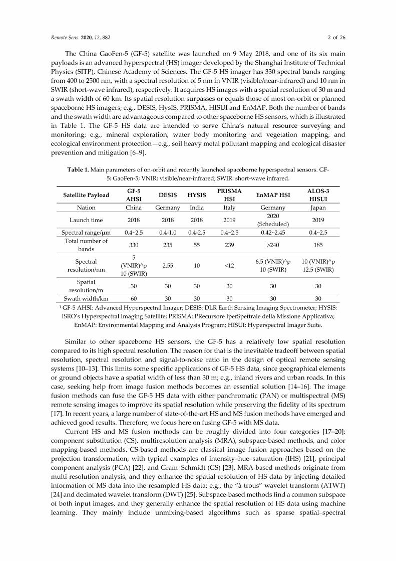
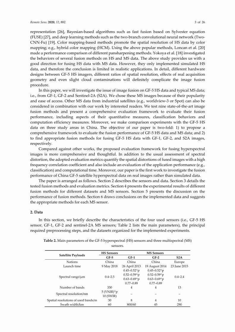
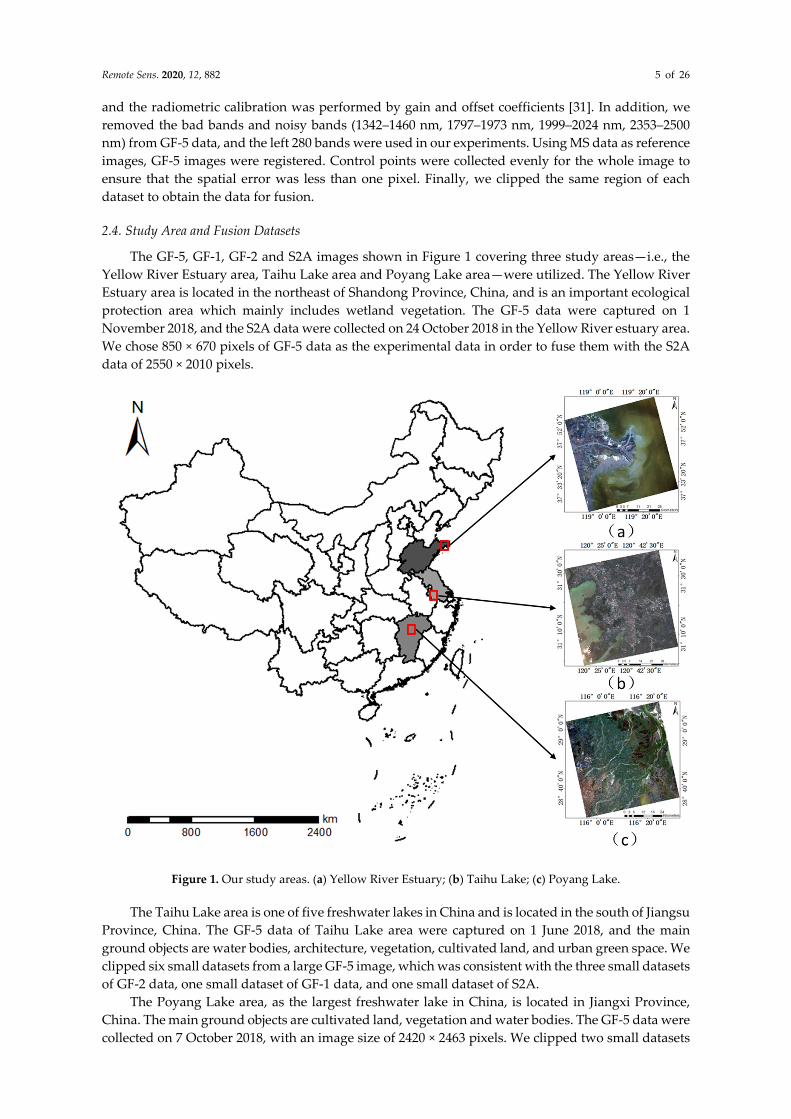
Fusing China GF 5 Hyperspectral Data with GF 1, GF 2 and ...

Remote Sens. 2020, 12, 882; doi:10.3390/rs12050882 www.mdpi.com/journal/remotesensing

Article

Fusing China GF‐5 Hyperspectral Data with GF‐1,

GF‐2 and Sentinel‐2A Multispectral Data: Which

Methods Should Be Used?

Kai Ren 1, Weiwei Sun 1, Xiangchao Meng 2,*, Gang Yang 1 and Qian Du 3

1 Department of Geography and Spatial Information Techniques, Ningbo University, Ningbo 315211, China;

[email protected] (K.R.); [email protected] (W.S.); [email protected] (G.Y.) 2 Faculty of Electrical Engineering and Computer Science, Ningbo University, Ningbo 315211, China 3 Department of Electrical and Computer Engineering, Mississippi State University, Starkville,

MS 39762, USA; [email protected]

* Correspondence: [email protected]; Tel.: +86‐187‐5832‐4997

Received: 7 February 2020; Accepted: 5 March 2020; Published: 9 March 2020

Abstract: The China GaoFen‐5 (GF‐5) satellite sensor, which was launched in 2018, collects

hyperspectral data with 330 spectral bands, a 30 m spatial resolution, and 60 km swath width. Its

competitive advantages compared to other on‐orbit or planned sensors are its number of bands,

spectral resolution, and swath width. Unfortunately, its applications may be undermined by its

relatively low spatial resolution. Therefore, the data fusion of GF‐5 with high spatial resolution

multispectral data is required to further enhance its spatial resolution while preserving its spectral

fidelity. This paper conducted a comprehensive evaluation study of fusing GF‐5 hyperspectral data

with three typical multispectral data sources (i.e., GF‐1, GF‐2 and Sentinel‐2A (S2A)), based on

quantitative metrics, classification accuracy, and computational efficiency. Datasets on three study

areas of China were utilized to design numerous experiments, and the performances of nine state‐

of‐the‐art fusion methods were compared. Experimental results show that LANARAS (this method

was proposed by lanaras et al.), Adaptive Gram–Schmidt (GSA), and modulation transfer function

(MTF)‐generalized Laplacian pyramid (GLP) methods are more suitable for fusing GF‐5 with GF‐1

data, MTF‐GLP and GSA methods are recommended for fusing GF‐5 with GF‐2 data, and GSA and

smoothing filtered‐based intensity modulation (SFIM) can be used to fuse GF‐5 with S2A data.

Keywords: hyperspectral remote sensing; GF‐5; GF‐1; GF‐2; S2A; data fusion

1. Introduction

Hyperspectral imaging sensors generally collect more than 100 spectral bands with a

wavelength range within 400–2500 nm. Because of their high spectral resolution, hyperspectral data

have achieved widespread applications in numerous research fields, such as in the fine classification

of ground objects. In recent years, hyperspectral remote sensing has developed rapidly. For example,

Italy launched the PRecursore IperSpettrale della Missione Applicativa (PRISMA) earth observation

satellite in March 2019 [1], Japan launched the Hyperspectral Imager Suite (HISUI) hyperspectral

satellite sensor in 2019 [2], India launched the ISRO’s Hyperspectral Imaging Satellite (HYSIS)

hyperspectral satellite in 2018 [3], and Germany launched the DLR Earth Sensing Imaging

Spectrometer (DESIS) hyperspectral satellite in 2018 and are planning to launch the Environmental

Mapping and Analysis Program (EnMAP) hyperspectral satellite in 2020 [4,5]. The development of

the hyperspectral satellite field will bring about new requirements for image processing.

Remote Sens. 2020, 12, 882 2 of 26

The China GaoFen‐5 (GF‐5) satellite was launched on 9 May 2018, and one of its six main

payloads is an advanced hyperspectral (HS) imager developed by the Shanghai Institute of Technical

Physics (SITP), Chinese Academy of Sciences. The GF‐5 HS imager has 330 spectral bands ranging

from 400 to 2500 nm, with a spectral resolution of 5 nm in VNIR (visible/near‐infrared) and 10 nm in

SWIR (short‐wave infrared), respectively. It acquires HS images with a spatial resolution of 30 m and

a swath width of 60 km. Its spatial resolution surpasses or equals those of most on‐orbit or planned

spaceborne HS imagers; e.g., DESIS, HysIS, PRISMA, HISUI and EnMAP. Both the number of bands

and the swath width are advantageous compared to other spaceborne HS sensors, which is illustrated

in Table 1. The GF‐5 HS data are intended to serve China’s natural resource surveying and

monitoring; e.g., mineral exploration, water body monitoring and vegetation mapping, and

ecological environment protection—e.g., soil heavy metal pollutant mapping and ecological disaster

prevention and mitigation [6–9].

Table 1. Main parameters of on‐orbit and recently launched spaceborne hyperspectral sensors. GF‐

5: GaoFen‐5; VNIR: visible/near‐infrared; SWIR: short‐wave infrared.

Satellite Payload GF‐5

AHSI DESIS HYSIS

PRISMA

HSI EnMAP HSI

ALOS‐3

HISUI

Nation China Germany India Italy Germany Japan

Launch time 2018 2018 2018 2019 2020

(Scheduled) 2019

Spectral range/μm 0.4~2.5 0.4‐1.0 0.4‐2.5 0.4~2.5 0.42~2.45 0.4~2.5

Total number of

bands 330 235 55 239 >240 185

Spectral

resolution/nm

5

(VNIR)^p

10 (SWIR)

2.55 10 <12 6.5 (VNIR)^p

10 (SWIR)

10 (VNIR)^p

12.5 (SWIR)

Spatial

resolution/m 30 30 30 30 30 30

Swath width/km 60 30 30 30 30 30 1 GF‐5 AHSI: Advanced Hyperspectral Imager; DESIS: DLR Earth Sensing Imaging Spectrometer; HYSIS:

ISRO’s Hyperspectral Imaging Satellite; PRISMA: PRecursore IperSpettrale della Missione Applicativa;

EnMAP: Environmental Mapping and Analysis Program; HISUI: Hyperspectral Imager Suite.

Similar to other spaceborne HS sensors, the GF‐5 has a relatively low spatial resolution

compared to its high spectral resolution. The reason for that is the inevitable tradeoff between spatial

resolution, spectral resolution and signal‐to‐noise ratio in the design of optical remote sensing

systems [10–13]. This limits some specific applications of GF‐5 HS data, since geographical elements

or ground objects have a spatial width of less than 30 m; e.g., inland rivers and urban roads. In this

case, seeking help from image fusion methods becomes an essential solution [14–16]. The image

fusion methods can fuse the GF‐5 HS data with either panchromatic (PAN) or multispectral (MS)

remote sensing images to improve its spatial resolution while preserving the fidelity of its spectrum

[17]. In recent years, a large number of state‐of‐the‐art HS and MS fusion methods have emerged and

achieved good results. Therefore, we focus here on fusing GF‐5 with MS data.

Current HS and MS fusion methods can be roughly divided into four categories [17–20]:

component substitution (CS), multiresolution analysis (MRA), subspace‐based methods, and color

mapping‐based methods. CS‐based methods are classical image fusion approaches based on the

projection transformation, with typical examples of intensity–hue–saturation (IHS) [21], principal

component analysis (PCA) [22], and Gram–Schmidt (GS) [23]. MRA‐based methods originate from

multi‐resolution analysis, and they enhance the spatial resolution of HS data by injecting detailed

information of MS data into the resampled HS data; e.g., the “à trous” wavelet transform (ATWT)

[24] and decimated wavelet transform (DWT) [25]. Subspace‐based methods find a common subspace

of both input images, and they generally enhance the spatial resolution of HS data using machine

learning. They mainly include unmixing‐based algorithms such as sparse spatial–spectral

Remote Sens. 2020, 12, 882 3 of 26

representation [26], Bayesian‐based algorithms such as fast fusion based on Sylvester equation

(FUSE) [27], and deep learning methods such as the two‐branch convolutional neural network (Two‐

CNN‐Fu) [19]. Color mapping‐based methods promote the spatial resolution of HS data by color

mapping; e.g., hybrid color mapping (HCM). Using the above popular methods, Loncan et al. [20]

made a performance comparison of different pansharpening methods. Yokoya et al. [18] investigated

the behaviors of several fusion methods on HS and MS data. The above study provides us with a

good direction for fusing HS data with MS data. However, they only implemented simulated HS

data, and therefore the conclusion is limited in realistic applications. In detail, different hardware

designs between GF‐5 HS imagers, different ratios of spatial resolution, effects of real acquisition

geometry and even slight cloud contaminations will definitely complicate the image fusion

procedure.

In this paper, we will investigate the issue of image fusion on GF‐5 HS data and typical MS data;

i.e., from GF‐1, GF‐2 and Sentinel‐2A (S2A). We chose these MS images because of their popularity

and ease of access. Other MS data from industrial satellites (e.g., worldview‐3 or Spot) can also be

considered in combination with our work by interested readers. We test nine state‐of‐the‐art image

fusion methods and present a comprehensive evaluation framework to evaluate their fusion

performance, including aspects of their quantitative measures, classification behaviors and

computation efficiency measures. Moreover, we make comparison experiments with the GF‐5 HS

data on three study areas in China. The objective of our paper is two‐fold: 1) to propose a

comprehensive framework to evaluate the fusion performance of GF‐5 HS data and MS data; and 2)

to find appropriate fusion methods for fusing GF‐5 HS data with GF‐1, GF‐2, and S2A images,

respectively.

Compared against other works, the proposed evaluation framework for fusing hyperspectral

images is more comprehensive and thoughtful. In addition to the usual assessment of spectral

distortion, the adopted evaluation metrics quantify the spatial distortions of fused images with a high

frequency correlation coefficient and also include an evaluation of the application performance (e.g.,

classification) and computational time. Moreover, our paper is the first work to investigate the fusion

performance of China GF‐5 satellite hyperspectral data on real images rather than simulated data.

The paper is arranged as follows. Section 2 describes the sensors and data. Section 3 details the

tested fusion methods and evaluation metrics. Section 4 presents the experimental results of different

fusion methods for different datasets and MS sensors. Section 5 presents the discussion on the

performance of fusion methods. Section 6 draws conclusions on the implemented data and suggests

the appropriate methods for each MS sensor.

2. Data

In this section, we briefly describe the characteristics of the four used sensors (i.e., GF‐5 HS

sensor, GF‐1, GF‐2 and sentinel‐2A MS sensors; Table 2 lists the main parameters), the principal

required preprocessing steps, and the datasets organized for the implemented experiments.

Table 2. Main parameters of the GF‐5 hyperspectral (HS) sensors and three multispectral (MS)

sensors.

Satellite Payloads HS Sensors MS Sensors

GF‐5 GF‐1 GF‐2 S2A

Nations China China China Europe

Launch time 9 May 2018 26 April 2013 19 August 2014 23 June 2015

Spectral range/μm 0.4–2.5

0.45–0.52^p

0.52–0.59^p

0.63–0.69^p

0.77–0.89

0.45–0.52^p

0.52–0.59^p

0.63–0.69^p

0.77–0.89

0.4–2.4

Number of bands 330 4 4 13

Spectral resolution/nm 5 (VNIR)^p

10 (SWIR) – – –

Spatial resolutions of used bands/m 30 8 4 10

Swath width/km 60 800/60 45 290

Remote Sens. 2020, 12, 882 4 of 26

2.1. GF‐5 Spaceborne Hyperspectral Sensor

The GF‐5 HS imager adopts convex grating spectrophotometry and has an elevated performance

with a three‐concentric‐mirror configuration. It includes two spectrometers and provides 330 spectral

bands (from 400 nm to 2500 nm) with 30 m spatial resolution (http://data.cresda.com). The VNIR

spectrometer has a spectral resolution of 5 nm, and the SWIR spectrometer has a spectral resolution

of 10 nm. Operating in a pushbroom fashion, the GF‐5 sensor has a swath width of 60 km. Moreover,

it optimizes the acquisition and processing techniques of weak signals, and the signal‐to‐noise ratio

(SNR) reaches 700 and 500 in VNIR and SWIR bands, respectively. By removing 50 severe water

absorption bands within 1350–1440 nm, 1800–1965 nm, and 2400–2500 nm, we utilize 280 bands from

the initial 330 bands to carry out our experiments, and the level of the products is L0.

2.2. GF‐1, GF‐2, and S2A Spaceborne Multispectral Sensors

GF‐1 satellite carries MS and PAN spectrometers, and it was launched on 26 April 2013 [28]. The

instruments adopt the time delay and integration (TDI) charge coupled device (CCD) imaging

technology to unify the five spectra and for the structural design of combining dual cameras. The GF‐

1 satellite carries four MS cameras and two PAN/MS cameras. These four MS sensors simultaneously

capture images with four bands and a 16 m spatial resolution, and the swath width reaches 800 km

through image mosaic technology. The PAN/MS cameras acquire PAN images with a 2 m spatial

resolution and MS images with 8 m spatial resolution and with a swath width of 60 km through

image mosaic technology. The GF‐1 instruments, which operate on the pushbroom principle, provide

VNIR bands but no SWIR bands. These acquired images of MS sensors cover the spectral ranges of

450–520 nm, 520–590 nm, 630–690 nm and 770–890 nm. In the experiment, we implement MS data

with a 8 m spatial resolution (http://data.cresda.com), and the level of the products is L1.

The GF‐2 satellite was launched on 19 August 2014, and it was equipped with two PAN/MS

cameras [29]. It adopts a long focal length, an advanced design of its optical system, and the TDI CCD

imaging technology to unify the five spectra. Operating in a pushbroom fashion, the instrument

collects one PAN band of 1 m spatial resolution and four MS bands (450–520 nm, 520–590 nm, 630–

690 nm, and 770–890 nm) of 4 m spatial resolution. The GF‐2 satellite optimizes the parameters of

orbit operation and skew maneuvering, and the field of view angle of 2.1° for a single camera is

realized to obtain a swath width of 45 km. We use the GF‐2 MS data with 4 m spatial resolution in

the experiment (http://data.cresda.com), and the level of the products is L1.

Sentinel‐2A is the second satellite of the Global Monitoring of Environment and Safety (GMES)

project in Europe, which was launched on 23 June 2015 [30]. It has a swath width of 290 km, and a

revisited period of 10 days. The instrument carries a MS imager covering 13 spectral bands with

different spatial resolutions (consisting of four bands of 10 m spatial resolution, six bands of 20 m

spatial resolution and three bands of 60 m spatial resolution), ranging from visible to short‐wave

infrared. In the optical field, the S2A data is the only source with three bands in the red‐edge range,

which is effective in monitoring the vegetation health status. The images with four bands and a 10 m

spatial resolution are used in our experiment, and the spectral ranges of these bands are 430–450 nm,

450–510 nm, 530–590 nm and 640–670 nm, respectively (https://scihub.copernicus.eu/dhus/#/home),

and the level of the products is L0.

2.3. Data Preprocessing

Before multi‐source data fusion, some data preprocessing work is essential, including ortho

correction, atmospheric correction, spatial registration, and image clipping. All data preprocessing

steps were carried out in ENVI software. These data sets were first converted into the world geodetic

system 1984 (WGS 1984) coordinate system. The global digital elevation model (DEM) data at 30 m

(https://asterweb.jpl.nasa.gov/gdem.asp) was used to correct the GF‐5 hyperspectral images and MS

images, and then the data were resampled using the rational polynomial coefficient files and the

bilinear interpolation method. All original images with digital numbers were calibrated to the surface

reflectance data. The Fast Line‐of‐Sight Atmosphere (FLAASH) module was performed for all data,

Remote Sens. 2020, 12, 882 5 of 26

and the radiometric calibration was performed by gain and offset coefficients [31]. In addition, we

removed the bad bands and noisy bands (1342–1460 nm, 1797–1973 nm, 1999–2024 nm, 2353–2500

nm) from GF‐5 data, and the left 280 bands were used in our experiments. Using MS data as reference

images, GF‐5 images were registered. Control points were collected evenly for the whole image to

ensure that the spatial error was less than one pixel. Finally, we clipped the same region of each

dataset to obtain the data for fusion.

2.4. Study Area and Fusion Datasets

The GF‐5, GF‐1, GF‐2 and S2A images shown in Figure 1 covering three study areas—i.e., the

Yellow River Estuary area, Taihu Lake area and Poyang Lake area—were utilized. The Yellow River

Estuary area is located in the northeast of Shandong Province, China, and is an important ecological

protection area which mainly includes wetland vegetation. The GF‐5 data were captured on 1

November 2018, and the S2A data were collected on 24 October 2018 in the Yellow River estuary area.

We chose 850 × 670 pixels of GF‐5 data as the experimental data in order to fuse them with the S2A

data of 2550 × 2010 pixels.

Figure 1. Our study areas. (a) Yellow River Estuary; (b) Taihu Lake; (c) Poyang Lake.

The Taihu Lake area is one of five freshwater lakes in China and is located in the south of Jiangsu

Province, China. The GF‐5 data of Taihu Lake area were captured on 1 June 2018, and the main

ground objects are water bodies, architecture, vegetation, cultivated land, and urban green space. We

clipped six small datasets from a large GF‐5 image, which was consistent with the three small datasets

of GF‐2 data, one small dataset of GF‐1 data, and one small dataset of S2A.

The Poyang Lake area, as the largest freshwater lake in China, is located in Jiangxi Province,

China. The main ground objects are cultivated land, vegetation and water bodies. The GF‐5 data were

collected on 7 October 2018, with an image size of 2420 × 2463 pixels. We clipped two small datasets

Remote Sens. 2020, 12, 882 6 of 26

from the large images of GF‐5 data: one was the Poyang Lake‐1 area with 600 × 500 pixel sizes, which

corresponds to GF‐1 data of a 2550 × 1875‐pixel size, and the other was the Poyang Lake‐2 area with

700 × 700 pixels that corresponds to S2A data of a 2100 × 2100‐pixel size. Table 3 lists the specific

information of these datasets fpr the three study areas.

Table 3. Specific information of the experimental datasets.

Datasets Area Sensors Time Image Size

GF‐5 and GF‐1

Taihu Lake‐1 GF‐5 HS 1 June 2018 540 × 300

GF‐1 MS 25 June 2018 2025 × 1125


GF‐1 MS 3 May 2018 1695 × 945

Poyang Lake‐1 GF‐5 HS 7 October 2018 600 × 500

GF‐1 MS 15 September 2018 2250 × 1875

GF‐5 and GF‐2


GF‐2 MS 14 May 2018 2685 × 1740


GF‐2 MS 14 May 2018 3375 × 1875


GF‐2 MS 14 May 2018 2715 × 1245

GF‐5 and S2A

Yellow River

Estuary

GF‐5 HS 1 November 2018 850 × 670

S2A MS 24 October 2018 2550 × 2010

Poyang Lake‐2 GF‐5 HS 7 October 2018 700 × 700

S2A MS 15 September 2018 2100 × 2100


S2A MS 4 May 2018 2250 × 1200

In order to explore the specific application performance of different fusion methods, the fused

images were classified and analyzed. By using Google Earth and field sampling, we obtained the

region of interest (ROI) for all land cover types. Tables 4–6 show the number of labeled samples in

each dataset. Training samples and testing samples were randomly selected from the selected ROI.

In order to ensure the classification accuracy, the number of testing samples was almost three times

that of training samples. All images were classified by using the support vector machine (SVM)

classifier in ENVI 5.3 software.

Table 4. Training and testing samples of each land cover type in all datasets (Taihu Lake‐1, Taihu

Lake‐2, Poyang Lake‐1). ROI: region of interest.

Land Cover

Types

Taihu Lake‐1 Taihu Lake‐2 Poyang Lake‐1

Training Testing Training Testing Training Testing

Pixel ROI Pixel ROI Pixel ROI Pixel ROI Pixel ROI Pixel ROI

River 315 70 923 100 265 60 523 100 203 60 465 100

Lake 232 20 633 36 193 20 325 30 265 50 512 100

Blue roof building 226 40 743 120 365 80 502 100 – – – – Bright roof

building 268 38 663 92 232 70 469 90 – – – –

Other building 369 50 904 100 295 70 378 100 195 50 368 80

Vegetation 236 30 669 80 102 20 232 50 – – – – Bare land 169 15 339 30 99 15 153 25 – – – – Swag 129 25 432 50 – – – – 134 50 433 80

Artificial trench – – – – 133 30 287 60 – – – – Tidal–flat area – – – – – – – – 169 65 364 100

Marsh – – – – – – – – 259 60 475 120

Dry land – – – – – – – – 169 45 295 80

Paddy field – – – – – – – – 187 55 368 100

Remote Sens. 2020, 12, 882 7 of 26

Table 5. Training and testing samples of each land cover type for datasets (Taihu Lake‐3, Taihu Lake‐

4, Taihu Lake‐5).

Land Cover

Types

Taihu Lake‐3 Taihu Lake‐4 Taihu Lake‐5



River 241 50 396 80 196 30 325 60 121 30 256 50

Lake 98 20 203 40 103 20 194 40 80 30 198 60

Blue roof building 125 80 206 160 134 75 214 140 89 60 167 120

Bright roof

building 93 60 162 90 98 50 183 90 98 50 179 100

Other building 135 80 265 160 150 85 299 150 131 70 199 135

Vegetation 90 30 265 50 93 25 169 40 90 30 204 60

Bare land 56 20 124 40 102 30 197 60 – – – – Red roof building 96 70 183 140 – – – – – – – –

Cement roof

building 126 80 268 160 – – – – – – – –

Asphat building 198 100 305 240 – – – – – – – – Farmland 65 20 93 50 – – – – – – – –

Artificial trench – – – – 111 60 261 110 – – – – Swag – – – – – – – – 256 142 756 269

Paddy field – – – – – – – – 304 100 661 200

Dry land – – – – – – – – 165 80 297 160

Table 6. Training and testing samples of each land cover type for datasets (Yellow River Estuary,

Poyang Lake‐2, Taihu Lake‐6).

Land Cover Types

Yellow River Estuary Poyang Lake‐2 Taihu Lake‐6



River 216 50 415 100 169 60 301 120 156 50 281 90

Lake – – – – 142 45 269 80 161 50 287 100

Suaeda salsa 221 80 325 100 – – – – – – – – Argillaceous beach 196 60 411 120 – – – – – – – –

River flat 203 75 412 100 – – – – – – – – Paddy field 156 80 296 160 – – – – 168 50 271 100

Reed 154 45 295 90 156 60 268 120 – – – – Non wetland 169 60 226 120 – – – – — — — —

Salt pan 167 80 301 160 – – – – — — — —

Other vegetation 235 75 421 140 – – – – 97 40 146 60

Swag 92 40 199 80 – – – – – – – – Paddy field – – – – 183 60 362 120 – – – –

Saline–alkali soil – – – – 189 80 268 140 – – – – Floating vegetation – – – – 169 50 258 100 – – – –

Yegu grass community – – – – 168 65 333 150 – – – – Road – – – – 87 40 161 90 – – – –

Dry land – – – – 81 40 152 80 88 50 117 80

Sandbank – – – – 134 60 251 120 – – – – Submerged vegetation – – – – 75 40 112 80 – – – – Artificial water body – – – – – – – – 185 60 288 120

Bare land – – – – – – – – 64 20 113 40

Blue roof building, – – – – – – – – 160 102 199 160

Bright roof building – – – – – – – – 175 100 287 200

other building – – – – 96 60 141 100 163 100 194 140

Remote Sens. 2020, 12, 882 8 of 26

3. Methods

3.1. The Study Framework

Figure 2 depicts the overall framework of our study, which consists of three main parts: (1) data

processing, (2) data fusion, and (3) the comprehensive evaluation of fused images. Some essential

steps are required for the data processing of GF‐5 HS data and MS data; i.e., radiation calibration,

atmospheric correction, image registration, and image clipping. The parameters of data fusion

methods were manually determined for different methods and different datasets. After that, the

performances of different fusion methods were evaluated by using comprehensive evaluation

measures; i.e., quantitative measures, application evaluation measures, and computational efficiency

measures. Finally, the behaviors of different methods for different datasets were analyzed (e.g.,

fusing GF‐5 and GF‐1, GF‐5 and GF‐2, GF‐5 and S2A) to summarize the appropriate fusion methods.

Figure 2. Flow chart of the implemented tests on image fusion methods. GSA: Adaptive Gram–

Schmidt (GSA); MTF‐GLP: Modulation transfer function‐generalized Laplacian pyramid; SFIM:

smoothing filtered‐based intensity modulation; CNMF: smoothing filtered‐based intensity

modulation; FUSE: fast fusion based on Sylvester equation; LANARAS: the method was proposed by

lanaras; MAP‐SMM: Maximum a posterior‐ stochastic mixing model; HCM: hybrid color mapping;

Two‐CNN‐Fu: Two‐branch Convolutional Neural Network.

3.2. Fusion Methods

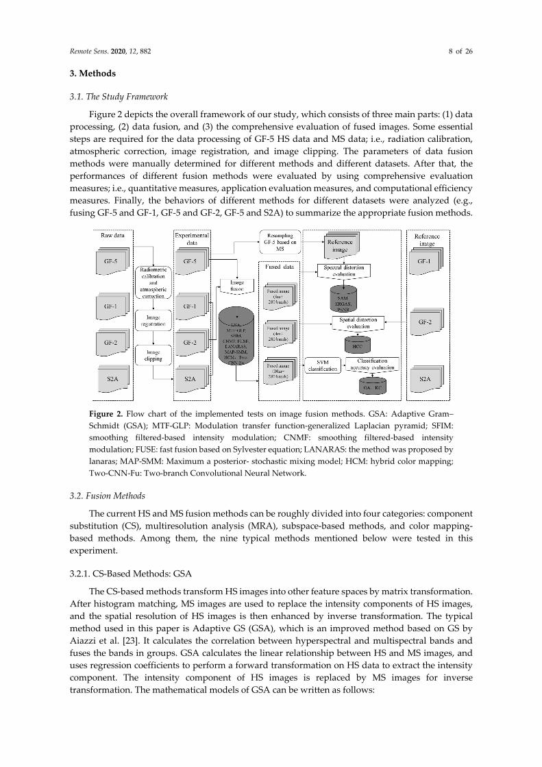
The current HS and MS fusion methods can be roughly divided into four categories: component

substitution (CS), multiresolution analysis (MRA), subspace‐based methods, and color mapping‐

based methods. Among them, the nine typical methods mentioned below were tested in this

experiment.

3.2.1. CS‐Based Methods: GSA

The CS‐based methods transform HS images into other feature spaces by matrix transformation.

After histogram matching, MS images are used to replace the intensity components of HS images,

and the spatial resolution of HS images is then enhanced by inverse transformation. The typical

method used in this paper is Adaptive GS (GSA), which is an improved method based on GS by

Aiazzi et al. [23]. It calculates the correlation between hyperspectral and multispectral bands and

fuses the bands in groups. GSA calculates the linear relationship between HS and MS images, and

uses regression coefficients to perform a forward transformation on HS data to extract the intensity

component. The intensity component of HS images is replaced by MS images for inverse

transformation. The mathematical models of GSA can be written as follows:

Remote Sens. 2020, 12, 882 9 of 26

𝐇𝐒 𝐇𝐒 𝐠 𝐌𝐒 𝐈 , 𝑖 1,⋯ ,𝑚; 𝑘 1,⋯ ,𝑛 (1)

𝐠𝑐𝑜𝑣 𝐈 ,𝐇𝐒

𝑣𝑎𝑟 𝐈 (2)

𝐈 𝐰 𝐇𝐒 (3)

where the subscript 𝑖 indicates the k‐th spectral band of the 𝑖th group data. 𝐇𝐒 and 𝐇𝐒 represent the fused image and the resampled hyperspectral image, respectively. 𝐌𝐒 is the i‐th multispectral

band. 𝐠 and 𝐰 are the forward transform coefficient and transform coefficient, respectively. 𝐈 represents the intensity component.

3.2.2. MRA‐Based Methods: MTF‐GLP and SFIM

The MRA‐based methods inject detail spatial features of MS images into resampled HS images

to enhance spatial resolution of HS data. A general formulation of MRA is given by

𝐇𝐒 𝐇𝐒 𝐚 𝐌𝐒 𝐌𝐒 , 𝑖 1,⋯ ,𝑚; 𝑘 1,⋯ ,𝑛 (4)

where 𝐌𝐒 represents the i‐th filtered multispectral band. 𝐚 is the gain coefficient of k‐th

hyperspectral band in the i‐th group data.

Two typical methods are Modulation transfer function(MTF)‐generalized Laplacian pyramid

(GLP) [32] and smoothing filtered‐based intensity modulation (SFIM) [33]. The MTF‐GLP categorizes

the bands of HS images into different groups according to the correlation coefficient between HS

bands and MS bands and enhances each group of HS images. It uses a Gaussian MTF filter to perform

low‐pass filtering for MS images. The high spatial detail image is obtained by subtracting filtered

images from the original MS data, and then the extracted detail image is injected into HS images by

using the global gain coefficient. SFIM is a fusion algorithm that formulates the relationship between

solar radiation and land surface reflection. It uses the same fusion steps to obtain detailed images as

MTF‐GLP; however, SFIM does not use the global gain, but uses the ratio between HS images and

low‐pass filter images of MS data as the gain coefficient. In SFIM and MTF‐GLP, 𝐚 is 𝐇𝐒

𝐌𝐒 and 1,

respectively.

3.2.3. Subspace‐Based Methods: CNMF, LANARAS, FUSE, MAP‐SMM and Two‐CNN‐FU

Subspace‐based methods mainly consist of Bayesian‐based approaches, unmixing‐based

approaches, and deep learning approaches. Bayesian‐based approaches enhance spatial resolution

by maximizing the posterior probability density of the full‐resolution images. We implemented two

typical Bayesian‐based approaches: i.e., fast fusion based on Sylvester equation (FUSE) and the

maximum a posteriori‐stochastic mixing model (MAP‐SMM) [34]. FUSE takes the original image as

a prior probability density, and it achieves image fusion by calculating the maximum posterior

probability density of the target image. It implements the alternating direction method of multipliers

(ADMM) [35] and block coordinate descent method [36] to merge prior information into the fusion

program. Moreover, it adopts the Sylvester equation [37] to give a close solution to the optimization

problem, which also greatly improves the computational efficiency. MAP‐SMM uses the stochastic

mixing model (SMM) [38] to evaluate the conditional mean vector and covariance matrix of HS

images relative to MS images, and obtains the mean spectrum, abundance map, and covariance

matrix of each endmember. After that, it establishes a maximum a posteriori (MAP) [39] function to

optimize the fused images and obtains the fused images by operating in the principal component

subspace of HS images. A general formulation of Bayesian based approaches is given by

𝑝 𝐇𝐒 ,𝐌𝐒 𝐇𝐒 𝑝 𝐇𝐒 |𝐇𝐒 𝑝 𝐌𝐒|𝐇𝐒 (5)

Remote Sens. 2020, 12, 882 10 of 26

where n is the number of data bands and i is the i‐th band of data. The maximum posterior probability

can be obtained by solving the following formula:

𝑙𝑜𝑔 𝑝 𝐇𝐒,𝐌𝐒 𝐇𝐒 𝑝 𝐇𝐒 𝐡 𝐣 (6)

𝐡𝐇�⃗� 𝐇�⃗�

2𝛅 (7)

𝐣∑ 𝛂 𝛻𝐇�⃗� 𝛻𝐌𝐒

2𝛅

𝛻𝐇�⃗�

𝐒 (8)

where 𝛅 represents the standard deviation of the error, Ω stands for an open interval, and S is a constant term.

Unmixing‐based methods decompose the HS and MS data into the HS basis and low‐resolution

coefficient matrix, MS basis and high‐resolution coefficients matrix, respectively. The resolution‐

enhanced HS images can be obtained by reconstructing the HS basis and high‐resolution coefficients.

The key formula is described as follows:

𝐇𝐒 𝐄𝐀 (9)

𝐇𝐒 𝐇𝐒𝐒 𝐄𝐀𝐒 𝐄𝐀 (10)

𝐌𝐒 𝐑𝐇𝐒 𝐑𝐄𝐀 𝐄𝐀 (11)

where E and A are the hyperspectral basis and high‐resolution coefficient matrix, respectively. S

represents the spatial response function, and R represents the spectral response function. Then, E and

A can be obtained by the minimum loss function:

𝑎𝑟𝑔𝑚𝑖𝑛𝐄,𝐀

𝐇𝐒 𝐄𝐀𝐒 𝐌𝐒 𝐑𝐄𝐀 (12)

where ‖∙‖ is the Frobenius norm. We implement two typical methods: i.e., the coupled nonnegative matrix factorization (CNMF)

[40] and LANARAS [41]. The CNMF, proposed by Naoto Yokoya et al., uses a nonnegative matrix

factorization (NMF) [42] to obtain the endmembers and abundances of HS and MS images. The fused

images are obtained by recombining the endmembers of HS images and the abundances of MS

images. CNMF uses vertex component analysis (VCA) [43] to calculate the initialized endmembers,

and the endmembers and abundances are iteratively updated through the minimum loss function.

LANARAS has similar fusion steps to CNMF, but it uses simplex identification via the split

augmented Lagrangian (SISAL) [44] to initialize the endmembers. It implements sparse unmixing by

variable splitting and the augmented Lagrangian [45] to initialize the abundance matrix and adopts

the projection gradient algorithm to update the endmember and abundance matrices of HS and MS

images.

Deep learning methods obtain the fused images through a neural network framework. The

trained framework includes high‐resolution HS (HRHS), high‐resolution MS (HRMS), and low

spatial resolution HS (LRHS). We implement one typical deep two‐branch convolutional neural

network (two‐CNN‐Fu). The formula is as follows:

𝐂 𝐕 ,𝐏 𝜕 𝐆 ∙ 𝛟 𝐪 (13)

𝝓 𝑪 𝑽 ⊕ 𝑪 𝑷 (14)

where 𝐂 𝐕 ,𝐏 is the output of the 𝑙 1 ‐th layer, 𝐂 𝐕 and 𝐂 𝐏 are the

extracted features of HS and MS data, respectively, 𝐆 is the weight matrix, and 𝐪 is the bias of

the fully connected (FC) layers. ⊕ represents the operation of concatenating HS features and the MS

features. The last FC layer is the spectrum of the fused image.

Remote Sens. 2020, 12, 882 11 of 26

3.2.4. Color Mapping‐Based Methods: HCM

Color mapping‐based methods enhance the spatial resolution of HS images by color mapping.

The conversion coefficient between data is calculated and the MS data is used for inverse

transformation to realize image fusion; the typical method we used is HCM [46]. The HCM obtains

the transformation matrix by using the linear relationship between downsampled MS images and HS

images, and utilizes the MS images and the transformation matrix to obtain the fused images. HCM

adds some bands of HS images into MS images and enhances the correlations between the resolution‐

reduced MS images and HS images. In addition, it adds a white band to compensate for the

atmospheric effect and other bias effects. The HCM is defined as

𝐇𝐒 𝐌𝐒 𝐇𝐒 ,⋯ 𝐁𝐚𝐧𝐝 𝐓∗ (15)

where 𝐇𝐒 ,⋯ represents the added bands of hyperspectral data, 𝐁𝐚𝐧𝐝 is the white band, T is

the transform coefficient, and the operation ∗ represents the transposition operation of the matrix.

𝐓∗ is defined as follows:

𝐓∗ 𝑎𝑟𝑔𝑚𝑖𝑛𝑻‖𝐇𝐒 𝐓𝐌𝐒‖ 𝜆‖𝐓‖ (16)

where ‖∙‖ is the Frobenius norm, and 𝜆 is a regularization parameter. The optimal 𝐓∗ is

𝐓∗ 𝐇𝐒 𝐌𝐒𝐓 𝐌𝐒 𝐌𝐒𝐓 𝜆𝐈 (17)

where 𝐈 is an identity matrix with the same dimension as 𝐌𝐒 𝐌𝐒𝐓.

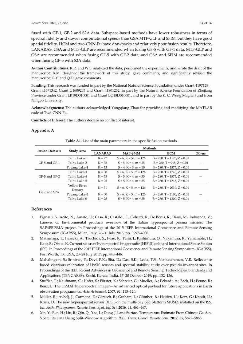
3.2.5. Parameter Settings

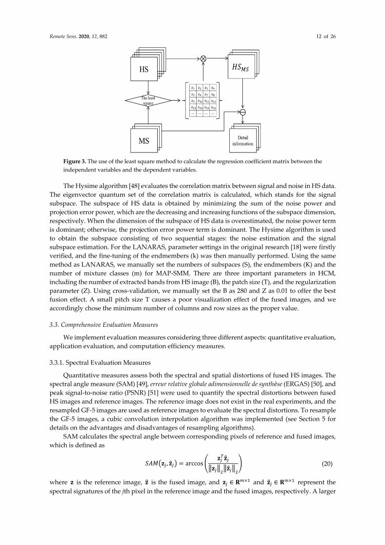
In the Appendix, Table A1 lists the main parameters of specific fusion methods. For SFIM and

MTF‐GLP, a synthetic image from MS images by regression coefficients is required to calculate the

detailed images. In these algorithms, the bands of HS data are the independent variables and the

bands of MS data are the dependent variables. Then, the least square method calculates the regression

coefficient matrix between the independent variables and the dependent variables by tge loss

function. The synthetic image is obtained by HS data multiplied by the coefficient matrix. Figure 3

shows the specific use of the least square method. In CNMF, the virtual dimensionality (VD)

algorithm [47] analyzes the typical eigenvalue of HS data by PCA and estimates the number of

spectrally distinct signal sources in the data. The number of spectrally distinct signal sources is the

initial number of endmembers (K). Based on the Neyman–Pearson hypothesis test, the VD algorithm

is as follows:

𝑘 𝑎𝑟𝑔𝑚𝑎𝑥 𝑃 𝜃 𝜇|𝜑 (18)

𝜗 𝑃 𝜃|𝜑 𝑑𝜃 (19)

where k is the number of endmembers, 𝜃 represents the output of the identification algorithm, and

𝜑 and 𝜑 are the alternate hypothesis and the null hypothesis, respectively. 𝜇 is a threshold that separates the two hypotheses, 𝜗 represents the desired false alarm density, and 𝑃 𝑥 represents the probability density function for k endmembers.

Remote Sens. 2020, 12, 882 12 of 26

Figure 3. The use of the least square method to calculate the regression coefficient matrix between the

independent variables and the dependent variables.

The Hysime algorithm [48] evaluates the correlation matrix between signal and noise in HS data.

The eigenvector quantum set of the correlation matrix is calculated, which stands for the signal

subspace. The subspace of HS data is obtained by minimizing the sum of the noise power and

projection error power, which are the decreasing and increasing functions of the subspace dimension,

respectively. When the dimension of the subspace of HS data is overestimated, the noise power term

is dominant; otherwise, the projection error power term is dominant. The Hysime algorithm is used

to obtain the subspace consisting of two sequential stages: the noise estimation and the signal

subspace estimation. For the LANARAS, parameter settings in the original research [18] were firstly

verified, and the fine‐tuning of the endmembers (k) was then manually performed. Using the same

method as LANARAS, we manually set the numbers of subspaces (S), the endmembers (K) and the

number of mixture classes (m) for MAP‐SMM. There are three important parameters in HCM,

including the number of extracted bands from HS image (B), the patch size (T), and the regularization

parameter (Z). Using cross‐validation, we manually set the B as 280 and Z as 0.01 to offer the best

fusion effect. A small pitch size T causes a poor visualization effect of the fused images, and we

accordingly chose the minimum number of columns and row sizes as the proper value.

3.3. Comprehensive Evaluation Measures

We implement evaluation measures considering three different aspects: quantitative evaluation,

application evaluation, and computation efficiency measures.

3.3.1. Spectral Evaluation Measures

Quantitative measures assess both the spectral and spatial distortions of fused HS images. The

spectral angle measure (SAM) [49], erreur relative globale adimensionnelle de synth�̀�se (ERGAS) [50], and peak signal‐to‐noise ratio (PSNR) [51] were used to quantify the spectral distortions between fused

HS images and reference images. The reference image does not exist in the real experiments, and the

resampled GF‐5 images are used as reference images to evaluate the spectral distortions. To resample

the GF‐5 images, a cubic convolution interpolation algorithm was implemented (see Section 5 for

details on the advantages and disadvantages of resampling algorithms).

SAM calculates the spectral angle between corresponding pixels of reference and fused images,

which is defined as

𝑆𝐴𝑀 𝐳 , 𝐳 arccos𝐳 𝐳

𝐳 𝐳 (20)

where 𝐳 is the reference image, 𝐳 is the fused image, and 𝐳 ∈ 𝐑 and 𝐳 ∈ 𝐑 represent the

spectral signatures of the jth pixel in the reference image and the fused images, respectively. A larger

Remote Sens. 2020, 12, 882 13 of 26

SAM means a more severe spectral distortion of the fused images. When the SAM equals 0, the fused

images have the smallest spectral distortion.

ERGAS is a global index for measuring spectral distortion, which is defined as

𝐸𝑅𝐺𝐴𝑆 𝐳, 𝐳 100𝑝1𝑚

∥ 𝐳 𝐳 ∥1𝑛 1 𝐳

(21)

where 𝐳 ∈ 𝐑 and 𝐳 ∈ 𝐑 represent the i-th band of the reference image and fused images,

respectively. 𝑝 is the ratio of the spatial resolution between MS and HS images, and n is the number

of pixels in the images. A larger ERGAS brings about more spectral distortion. When ERGAS is equal

to 0, the spectral distortion is the smallest.

PSNR is the ratio of the maximum power of a signal to the noise power that affects its

representational accuracy. It evaluates the reconstruction error of fused images, which is defined as

𝑃𝑆𝑁𝑅 𝐳 , 𝐳 10 ∙ 𝑙𝑜𝑔𝑚𝑎𝑥 𝐳

∥ 𝐳 𝐳 ∥ 𝑛⁄ (22)

where 𝑚𝑎𝑥 𝐳 is the maximum value in the ith band of the reference image, in which a higher PSNR

means a better result.

3.3.2. Spatial Evaluation Measures

Meanwhile, the high‐frequency correlation coefficient (HCC) was utilized to measure spatial

distortion. We adopt edge detection technology to extract edge information from MS images and

fused images, respectively. Taking the edge detection results of MS images as the reference images,

the correlation coefficients between the detection maps of fused images and MS images are

calculated. We use the Sobel operator to extract the edge information. The HCC is defined as

𝐻𝐶𝐶 𝐀,𝐁∑ 𝐀 𝐀 𝐁 𝐁

∑ 𝐀 𝐀 ∑ 𝐁 𝐁

(23)

where A and B are the reference edge images and the evaluated edge images, respectively; 𝐀 and 𝐁 are the samples of 𝐀 and 𝐁; e is the total number of the samples; and 𝐀 and 𝐁 are the means of

A and B. The ideal value of HCC is 1.

3.3.3. Classification Evaluation Measures

The overall accuracy (OA) [52] and Kappa coefficient (KC) [53] are used to quantify the

classification accuracy of fused images and evaluate the application performance. OA is a commonly

used indicator for evaluating the behaviors of image classification, which is defined as

𝑂𝐴∑ 𝐗𝐮

(24)

where 𝑤 is the number of classes, u represents the total number of samples, and 𝐗 represents the

observation in row i and column i. A higher OA means a better classification result.

KC is another reliable indicator for the accuracy evaluation of image classification. The formula

is defined as follows:

𝐾𝐶𝐮∑ 𝐗 ∑ 𝐗 𝐗

𝐮 ∑ 𝐗 𝐗 (25)

where 𝐗 and 𝐗 represent the marginal total in row i and column i, respectively. The range of KC

is between 0 and 1, and a larger KC means higher classification accuracy.

Remote Sens. 2020, 12, 882 14 of 26

3.3.4. Computational Efficiency Measures

The running time is recorded to evaluate the computational efficiency of different fusion

methods. All the fusion methods are implemented in MATLAB 2016a, and their codes are run on a

WIN10 computer with Intel Core i7 processor and 64 GB RAM.

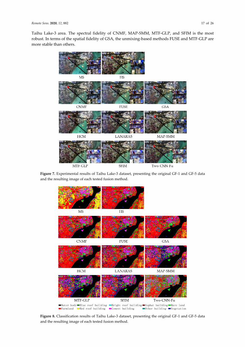
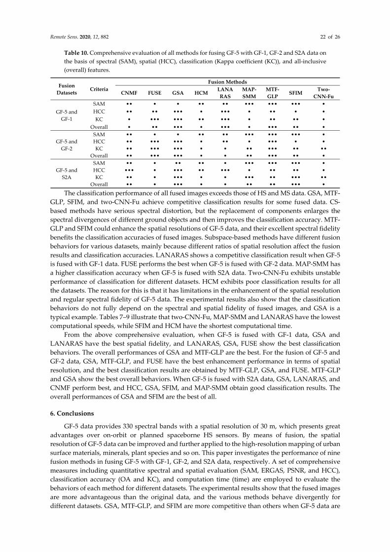
4. Results

4.1. Fusion Results of GF‐5 and GF‐1

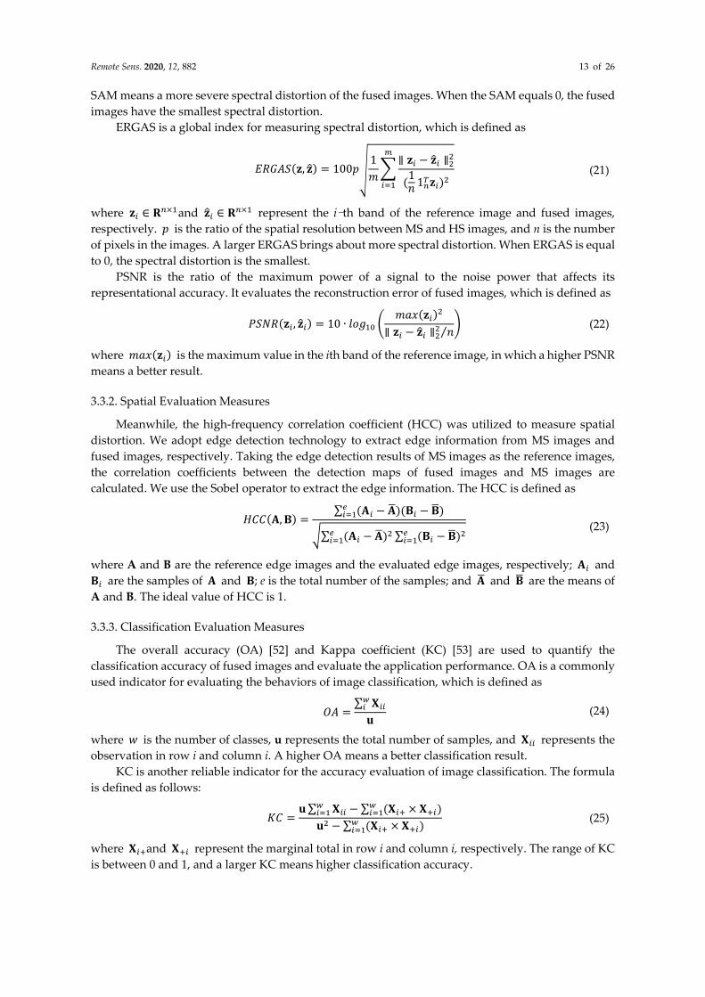
Table 7 describes the quantitative evaluation results of fused images from GF‐5 and GF‐1 data.

The bold type represents the best result, and the second‐best result is underlined. Figure 4 shows the

fused image of nine methods for the Taihu lake‐1 dataset. The observations in Table 7 and Figure 4

show the robustness of GSA, CNMF, LANARAS, and FUSE in terms of spatial fidelity. The reason

for this is that GSA injects spatial details of MS data into HS data via component substitution and has

an ideal transformation coefficient to maintain the spectral separation of HS data. The two unmixing‐

based methods and FUSE formulate the relationships between HS data, MS data, and fused images,

and implement the minimum loss function to reduce the approximation error while eliminating the

effects of noise. It is interesting that FUSE has good spectral fidelity in the Poyang Lake‐1 dataset,

whereas it suffers serious spectral distortion in the Taihu Lake‐1 area and Taihu Lake‐2 area. Our

assumed reason for this is that the Hysime is unsuitable for identifying the subspaces of data in

complicated building areas. MTF‐GLP, SFIM and MAP‐SMM have good spectral fidelity, but SFIM

and MAP‐SMM have severe spatial distortion. MRA‐based methods obtain detailed information by

filtering MS data in the fusion process. They inject detailed information into HS data with the gain

coefficient, and the spectral information of HS data is not modified in the fused images. In contrast,

the gain coefficient of SFIM is not as ideal as that of MTF‐GLP, resulting in an insufficient injection

of spatial details in SFIM. The number of endmembers in MAP‐SMM affects the behaviors of SMM

and accordingly limits the enhancement of spatial resolution of HS data [18].

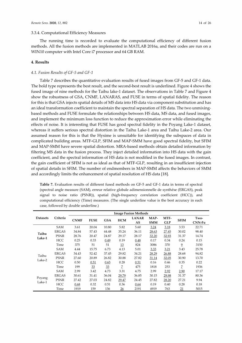
Table 7. Evaluation results of different fused methods on GF‐5 and GF‐1 data in terms of spectral

(spectral angle measure (SAM), erreur relative globale adimensionnelle de synth�̀�se (ERGAS), peak signal to noise ratio (PSNR)), spatial (high‐frequency correlation coefficient (HCC)), and

computational efficiency (Time) measures. (The single underline value is the best accuracy in each

case, followed by double underline.)

Datasets Criteria

Image Fusion Methods

CNMF FUSE GSA HCM LANAR

AS

MAP‐

SMM

MTF‐

GLP SFIM

Two‐

CNN‐Fu

Taihu

Lake‐1

SAM 3.61 20.04 10.80 5.82 5.60 3.24 3.18 3.53 22.71

ERGAS 34.84 57.43 44.48 35.24 36.11 28.63 27.45 30.02 98.40

PSNR 28.76 20.47 24.87 29.17 28.17 32.20 32.93 31.37 14.74

HCC 0.25 0.33 0.49 0.19 0.48 0.17 0.34 0.24 0.15

Time 375 51 51 13 824 3086 370 9 3150

Taihu

Lake‐2

SAM 4.44 15.75 6.73 4.13 5.01 3.33 3.21 3.43 25.78

ERGAS 34.43 52.42 37.45 29.82 34.21 28.29 26.88 28.68 94.82

PSNR 27.60 20.89 26.82 30.88 27.82 31.14 32.05 30.90 13.70

HCC 0.50 0.51 0.65 0.28 0.51 0.16 0.46 0.35 0.22

Time 199 33 33 7 475 1818 253 7 1936

Poyang

Lake‐1

SAM 2.99 3.42 4.73 3.31 4.75 2.99 2.92 2.90 17.17

ERGAS 30.61 31.41 36.04 29.79 36.85 30.15 29.98 31.37 80.36

PSNR 27.42 27.03 24.82 29.47 24.45 27.82 28.20 27.21 9.94

HCC 0.68 0.32 0.51 0.36 0.64 0.19 0.40 0.28 0.18

Time 1919 159 136 26 2191 4919 763 21 5015

Remote Sens. 2020, 12, 882 15 of 26

Figure 4. Experimental results of the Taihu Lake‐1 dataset, presenting the original GF‐1 and GF‐5 data

and the resulting image of each tested fusion method.

HCM has good visualization behaviors but has severe spatial distortion and regular spectral

fidelity. It adds some bands of HS data into MS data, and the spatial resolutions of these added bands

are not well enhanced by color mapping. The fused images accordingly preserve all spectral

information of MS data but only part of the spectral information of HS data. In two‐CNN‐Fu, due to

the lack of HRHS, the spectral response function was used to downsample the HS as HRMS, the

Gauss fuzzy kernel and point distribution function were used to calculate HS to get LRHS, and the

original HS is used as HRHS. In the experiment, the neural network framework was trained by using

the simulation data set, which made the trained neural network framework have great defects, and

the image with the worst fusion effect was obtained.

Figure 5 shows an example of the classification results, and Figure 6 plots the classification

accuracy of all fused images on the three datasets (see Table 4 for the categories of objects). The KC

and OA of fused images are higher than those of HS and MS data. All fused images obtain similar

and good classification behaviors in Poyang Lake‐1, and their classification performances diverge

greatly for the Taihu Lake‐1 and Lake‐2 datasets. We guessed that their divergent performances result

from different land covers in the three datasets. The building areas in Taihu Lake‐1 and Lake‐2 have

complicated spectral information and rich spatial detail, which demonstrates the behaviors of

different fusion methods. GSA, FUSE and LANARAS have higher classification accuracies, SFIM,

MAP‐SMM, HCM and two‐CNN‐Fu have the worst KC and OA, and MTF‐GLP and CNMF are

unstable.

Remote Sens. 2020, 12, 882 16 of 26

Figure 5. Classification results of the Taihu Lake‐1 dataset, presenting the original GF‐1 and GF‐5 data


Figure 6. Classification accuracy of GF‐1, GF‐5 and fused images. (a) Taihu Lake‐1 area. (b) Taihu

Lake‐2 area. (c) Poyang Lake‐1 area.

4.2. Fusion Results of GF‐5 and GF‐2

As shown in Table 8 and Figure 7, GSA, the unmixing‐based methods—FUSE and MTF‐GLP—

show robustness in terms of spatial fidelity when fusing GF‐5 data with GF‐2 data (see the detail on

the Taihu Lake‐3 dataset in Figures 7 and 8). MAP‐SMM, MTF‐GLP, and SFIM exhibit less spectral

distortion, while HCM and two‐CNN‐Fu has severe spatial distortions and regular spectral fidelity.

However, compared with those of GF‐5 data and GF‐1 data, the SAMs of all fused images increase.

A larger ratio of spatial resolution between GF‐5 and GF‐2 data requires more pixels of GF‐2 data to

be obtained to perform the image interpolation in the fusion process. That would involve more

heterogenous pixels and then cause the spectral distortion of HS data. Except for two‐CNN‐Fu, all

fusion methods have good spectral fidelity in the Taihu Lake‐4 and Lake‐5 areas. Except for CNMF,

MAP‐SMM, MTF‐GLP and SFIM, the other five methods have serious spectral distortions in the

Remote Sens. 2020, 12, 882 17 of 26

Taihu Lake‐3 area. The spectral fidelity of CNMF, MAP‐SMM, MTF‐GLP, and SFIM is the most

robust. In terms of the spatial fidelity of GSA, the unmixing‐based methods FUSE and MTF‐GLP are

more stable than others.

Figure 7. Experimental results of Taihu Lake‐3 dataset, presenting the original GF‐1 and GF‐5 data


Figure 8. Classification results of Taihu Lake‐3 dataset, presenting the original GF‐1 and GF‐5 data


Remote Sens. 2020, 12, 882 18 of 26

Table 8. Evaluation results of different fused methods on GF‐5 and GF‐2 data in terms of spectral

(SAM, ERGAS, PSNR), spatial (HCC), and computational efficiency (Time) measures. (The single

underline value is the best accuracy in each case, followed by double underline.)

Datasets Criteria


CNMF FUSE GSA HCM LANA

RAS

MAP‐

SMM

MTF‐

GLP SFIM

Two‐

CNN‐Fu

Taihu

Lake‐3

SAM 4.50 14.17 8.06 6.09 6.63 3.82 3.56 3.75 30.23

ERGAS 38.70 48.12 39.13 34.47 37.93 29.32 28.56 30.13 75.11

PSNR 23.54 21.15 24.16 27.05 24.72 29.28 29.65 28.70 12.01

HCC 0.60 0.53 0.59 0.33 0.49 0.29 0.51 0.40 0.21

Time 489 124 112 40 2908 2954 358 24 2988

Taihu

Lake‐4

SAM 4.61 7.95 6.87 4.48 5.84 3.85 4.02 4.22 28.11

ERGAS 37.77 40.69 37.87 30.55 35.53 30.32 30.07 31.63 76.05

PSNR 25.77 24.80 26.37 29.32 27.22 29.93 30.18 29.26 14.72

HCC 0.52 0.69 0.69 0.23 0.55 0.30 0.57 0.46 0.21

Time 625 216 158 35 6301 4496 476 26 4502

Taihu

Lake‐5

SAM 3.73 6.85 6.00 4.70 5.41 3.40 3.40 3.60 26.85

ERGAS 38.01 39.51 36.84 31.95 37.42 29.95 29.90 31.76 75.36

PSNR 27.27 26.31 27.90 31.13 28.32 31.59 31.74 30.71 13.64

HCC 0.49 0.60 0.58 0.21 0.46 0.30 0.47 0.38 0.18

Time 357 83 74 22 3376 2127 259 12 2994

An example of classification results is shown in Figure 8, and Figure 9 plots the classification

accuracy of GF‐5 data, GF‐2 data and all fused images (see Table 5 for the categories of objects).

Similar to Figure 4, the fused images show better behaviors than the original HS data and MS data.

SFIM and MAP‐SMM show relatively poor classification accuracy in Taihu Lake‐4, while the other

methods always achieve similar and robust classification results. GSA, FUSE and MTF‐GLP have

better classification accuracies when GF‐5 data are fused with GF‐2 data.

Figure 9. Classification accuracy of GF‐2, GF‐5 and fused images. (a) Taihu Lake‐3 area. (b) Taihu

Lake‐4 area. (c) Taihu Lake‐5 area.

4.3. Fusion Results of GF‐5 and S2A

Table 9 shows the evaluation results and fused images of all nine methods for GF‐5 and S2A

data. Compared with GF‐2 and GF‐1 data, the divergences of SAM from the nine fused images are

smaller. The explanation for that is that GF‐5 and S2A data have a smaller ratio of spatial resolutions.

GSA and unmixing‐based methods show more robustness in the spatial fidelity.

Table 9. Evaluation results of different fused methods on GF‐5 and S2A data in terms of spectral

(SAM, ERGAS, PSNR), spatial (HCC), and computational efficiency (Time) measures. (The single

underline value is the best accuracy in each case, followed by double underline.)

Datasets Criteria



RAS

MAP‐

SMM

MTF‐

GLP SFIM

Two‐

CNN‐Fu

Remote Sens. 2020, 12, 882 19 of 26

Yellow

River

Estuary

SAM 2.09 5.55 3.30 0.99 4.51 1.43 1.31 1.39 34.65

ERGAS 33.22 30.27 28.60 16.19 48.16 20.07 19.61 20.73 79.18

PSNR 22.36 24.74 25.87 36.87 21.26 32.22 32.61 31.66 7.27

HCC 0.58 0.25 0.55 0.14 0.66 0.13 0.34 0.27 0.26

Time 1479 91 154 37 1836 8886 638 23 9543

Poyang

Lake‐2

SAM 3.23 3.15 3.95 4.34 4.67 2.45 2.27 1.52 22.85

ERGAS 31.29 29.45 34.50 32.57 35.89 26.64 26.16 24.85 80.70

PSNR 26.56 27.61 25.23 26.96 24.31 29.40 29.83 30.39 9.61

HCC 0.56 0.24 0.55 0.37 0.66 0.21 0.36 0.27 0.33

Time 2587 53 96 17 1545 7594 476 17 7975

Taihu

Lake‐6

SAM 3.26 6.31 5.85 4.58 5.34 3.32 3.42 3.53 26.65

ERGAS 37.71 36.88 35.09 30.83 35.39 28.18 27.89 29.18 75.53

PSNR 26.28 26.94 28.17 30.65 27.74 31.68 31.88 31.08 14.23

HCC 0.72 0.76 0.79 0.63 0.74 0.32 0.47 0.42 0.38

Time 478 41 74 15 3600 4635 326 13 5103

In the Yellow River Estuary area and Poyang Lake‐2 area, FUSE has severe spatial distortion,

but the enhancement of spatial resolution is obvious in the Taihu Lake‐6 area (for detail, see Figure

10). Two‐CNN‐Fu has the worst fidelity in both spatial and spectral aspects. HCM could preserve the

spectral information of MS data and part of the spectral information of HS data during the fusion

process. It achieves the best spectral fidelity in Yellow River Estuary, but has relatively regular

performance in terms of spectral fidelity on the Poyang Lake‐2 and Taihu Lake‐6 datasets. The reason

for this is that different time lags in collection data make the spectral divergence of GF‐5 and S2A in

the Yellow River Estuary smaller than those in Poyang Lake‐2 and Taihu Lake‐6.

Figure 10. Experimental results of Taihu Lake‐6 dataset, presenting the original GF‐1 and GF‐5 data


Remote Sens. 2020, 12, 882 20 of 26

Figure 11. Classification results of Taihu Lake‐6 dataset, presenting the original GF‐1 and GF‐5 data


Figure 12. Classification accuracy of S2A, GF‐5 and fused images. (a) Yellow River Estuary area. (b)

Poyang Lake‐2 area. (c) Taihu Lake‐6 area.

An example of classification results is shown in Figure 11, and Figure 12 plots the OA and KC

of GF‐5, S2A data and all fused images (see Table 6 for the categories of objects). The classification

results of the fused images are superior to the original HS data and MS data. GSA, SFIM, MAP‐SMM

and two‐CNN‐Fu have the best classification performance, with the highest OA and KC. The

classification accuracies of MTF‐GLP, FUSE, CNMF, LANARAS and HCM are unstable, and these

methods perform better for Taihu Lake‐6 than in the Yellow River Estuary and Poyang Lake‐2 areas.

5. Discussion

In this paper, we propose a comprehensive evaluation framework, which is very effective in

comparing the current fusion methods. Although our predecessors have undertaken several

corresponding works—for example, in 2014, Vivone et al. conducted a comparative analysis on the

Remote Sens. 2020, 12, 882 21 of 26

methods of MS pansharpening—they only used quantitative indicators to evaluate various methods

[17]. Loncan et al. conducted a comparative analysis of the HS pansharpening methods in 2015 and

conducted a quantitative evaluation of several methods [20], and the computational efficiency of

various methods was also evaluated. In 2017, Yokoya et al. evaluated various HS and MS fusion

approaches from a quantitative and applied perspective [18]. However, our evaluation framework

adds HCC evaluation indicators, which can effectively evaluate the spatial distortion of various

methods, which was not the case in previous literature. Our framework simultaneously evaluates

spectral distortion, spatial distortion, application performance, and computational efficiency. In

addition, previous papers used simulation datasets to evaluate various methods, but we used real

datasets to verify the performance of different methods, which led to a more objective evaluation

result.

In this experiment, real datasets were used for fusion, and resampled HS data were used as

reference data to evaluate the fused data. Therefore, we summarized and analyzed the existing image

interpolation methods. The current image interpolation methods mainly include nearest neighbor

interpolation [54], bilinear interpolation [55], and cubic convolution interpolation [56]. The advantage

of the nearest neighbor interpolation method is that the calculation is very small and the operation

speed is fast. However, it only uses the gray value of the pixel closest to the sampling point to be

tested as the gray value of the sampling point, without considering the influence of other neighboring

pixel points. Therefore, after resampling, the gray value has obvious discontinuity, the image quality

loss is large, and there will be obvious mosaic and saw tooth phenomena [57]. Bilinear interpolation

is better than nearest neighbor interpolation, but the calculation is a little large, the algorithm is more

complex, and the computational time of the program is a little long. The image quality after zooming

is high, which basically overcomes the feature of the discontinuous gray value of nearest neighbor

interpolation. The reason for this is that it considers the influence of four direct neighbors around the

sampling point to be tested on the correlation of the sampling point. However, this method only

considers the influence of the gray values of the four direct neighboring points around the testing

sample, and it does not include the influence of the change rate of the gray value between the

neighboring points. Accordingly, it has the property of a low‐pass filter, which leads to the loss of the

high‐frequency components of the image after scaling, and the image edge becomes fuzzier to a

certain extent. Compared with the input image, the output image after zooming by this method still

has the problems of image quality damage and low calculation accuracy due to the poor

consideration of interpolation function design [58]. Cubic convolution interpolation is the most

widely used algorithm. It not only considers the influence of the gray values of the four neighboring

pixels but also considers the influence of the change rate of their gray values. Therefore, it overcomes

the shortcomings of the former two methods, with generally smoother edges than bilinear

interpolation and high calculation accuracy [59].

Besides this, the performance of each fusion method was discussed comprehensively when

fusing GF‐5 data with GF‐1, GF‐2 and S2A data, respectively. In Table 10, more points indicate better

fusion performance. By adding the scores of each method in SAM, HCC and KC, this comprehensive

score result in overall terms is obtained.

When fusing GF‐5 with three typical MS data sources, the spatial resolution enhancement of

GSA is obvious when replacing intensity components of HS data, and spectral distortion is also

caused during the image fusion process. MAP‐SMM, MTF‐GLP, and SFIM have better performance

in terms of spectral fidelity, and MTF‐GLP behaves well when enhancing the spatial resolution.

However, MAP‐SMM is sensitive to the number of endmembers, and SFIM is affected by the gain

coefficient, which limits their performance in image fusion. HCM simultaneously preserves the

spectral information of MS data and HS data by color mapping. However, the added bands have

poor behaviors in spatial resolution enhancement, and that causes HCM to have clear defects. Two‐

CNN‐Fu has the worst spectral and spatial fidelity for all datasets.

Remote Sens. 2020, 12, 882 22 of 26

Table 10. Comprehensive evaluation of all methods for fusing GF‐5 with GF‐1, GF‐2 and S2A data on

the basis of spectral (SAM), spatial (HCC), classification (Kappa coefficient (KC)), and all‐inclusive

(overall) features.

Fusion

Datasets Criteria

Fusion Methods


RAS

MAP‐

SMM

MTF‐

GLP SFIM

Two‐

CNN‐Fu

GF‐5 and

GF‐1

SAM •• • • •• •• ••• ••• ••• •

HCC •• •• ••• • ••• • •• • •

KC • ••• ••• •• ••• • •• •• •

Overall • •• ••• • ••• • ••• •• •

GF‐5 and

GF‐2

SAM •• • • •• •• ••• ••• ••• •

HCC •• ••• ••• • •• • ••• • •

KC •• ••• ••• • • •• ••• •• ••

Overall •• ••• ••• • • •• ••• •• •

GF‐5 and

S2A

SAM •• • •• •• • ••• ••• ••• •

HCC ••• • ••• •• ••• • •• •• •

KC •• • ••• • • ••• •• ••• ••

Overall •• • ••• • • •• •• ••• •

The classification performance of all fused images exceeds those of HS and MS data. GSA, MTF‐

GLP, SFIM, and two‐CNN‐Fu achieve competitive classification results for some fused data. CS‐

based methods have serious spectral distortion, but the replacement of components enlarges the

spectral divergences of different ground objects and then improves the classification accuracy. MTF‐

GLP and SFIM could enhance the spatial resolutions of GF‐5 data, and their excellent spectral fidelity

benefits the classification accuracies of fused images. Subspace‐based methods have different fusion

behaviors for various datasets, mainly because different ratios of spatial resolution affect the fusion

results and classification accuracies. LANARAS shows a competitive classification result when GF‐5

is fused with GF‐1 data. FUSE performs the best when GF‐5 is fused with GF‐2 data. MAP‐SMM has

a higher classification accuracy when GF‐5 is fused with S2A data. Two‐CNN‐Fu exhibits unstable

performance of classification for different datasets. HCM exhibits poor classification results for all

the datasets. The reason for this is that it has limitations in the enhancement of the spatial resolution

and regular spectral fidelity of GF‐5 data. The experimental results also show that the classification

behaviors do not fully depend on the spectral and spatial fidelity of fused images, and GSA is a

typical example. Tables 7–9 illustrate that two‐CNN‐Fu, MAP‐SMM and LANARAS have the lowest

computational speeds, while SFIM and HCM have the shortest computational time.

From the above comprehensive evaluation, when GF‐5 is fused with GF‐1 data, GSA and

LANARAS have the best spatial fidelity, and LANARAS, GSA, FUSE show the best classification

behaviors. The overall performances of GSA and MTF‐GLP are the best. For the fusion of GF‐5 and

GF‐2 data, GSA, MTF‐GLP, and FUSE have the best enhancement performance in terms of spatial

resolution, and the best classification results are obtained by MTF‐GLP, GSA, and FUSE. MTF‐GLP

and GSA show the best overall behaviors. When GF‐5 is fused with S2A data, GSA, LANARAS, and

CNMF perform best, and HCC, GSA, SFIM, and MAP‐SMM obtain good classification results. The

overall performances of GSA and SFIM are the best of all.

6. Conclusions

GF‐5 data provides 330 spectral bands with a spatial resolution of 30 m, which presents great

advantages over on‐orbit or planned spaceborne HS sensors. By means of fusion, the spatial

resolution of GF‐5 data can be improved and further applied to the high‐resolution mapping of urban

surface materials, minerals, plant species and so on. This paper investigates the performance of nine

fusion methods in fusing GF‐5 with GF‐1, GF‐2, and S2A data, respectively. A set of comprehensive

measures including quantitative spectral and spatial evaluation (SAM, ERGAS, PSNR, and HCC),

classification accuracy (OA and KC), and computation time (time) are employed to evaluate the

behaviors of each method for different datasets. The experimental results show that the fused images

are more advantageous than the original data, and the various methods behave divergently for

different datasets. GSA, MTF‐GLP, and SFIM are more competitive than others when GF‐5 data are

Remote Sens. 2020, 12, 882 23 of 26

fused with GF‐1, GF‐2 and S2A data. Subspace‐based methods have lower robustness in terms of

spectral fidelity and slower computational speeds than GSA MTF‐GLP and SFIM, but they have good

spatial fidelity. HCM and two‐CNN‐Fu have drawbacks and relatively poor fusion results. Therefore,

LANARAS, GSA and MTF‐GLP are recommended when fusing GF‐5 with GF‐1 data, MTF‐GLP and

GSA are recommended when fusing GF‐5 with GF‐2 data, and GSA and SFIM are recommended

when fusing GF‐5 with S2A data.

Author Contributions: K.R. and W.S. analyzed the data, performed the experiments, and wrote the draft of the

manuscript; X.M. designed the framework of this study, gave comments, and significantly revised the

manuscript; G.Y. and Q.D. gave comments.

Funding: This research was funded in part by the National Natural Science Foundation under Grant 4197129，

Grant 41671342, Grant U1609203 and Grant 41801252, in part by the Natural Science Foundation of Zhejiang

Province under Grant LR19D010001 and Grant LQ18D010001, and in part by the K. C. Wong Magna Fund from

Ningbo University.

Acknowledgments: The authors acknowledged Yongqiang Zhao for providing and modifying the MATLAB

code of Two‐CNN‐Fu.

Conflicts of Interest: The authors declare no conflict of interest.

Appendix A

Table A1. List of the main parameters in the specific fusion methods.

Fusion Datasets Study Area Methods

LANARAS MAP‐SMM HCM Others

GF‐5 and GF‐1

Taihu Lake‐1 K = 27 S = 6, K = 5, m = 126 B = 280, T = 1125, Z = 0.01

Taihu Lake‐2 K = 35 S = 5, K = 4, m = 35 B = 280, T = 945, Z = 0.01 —

Poyang Lake‐1 K = 33 S = 4, K = 3, m = 10 B = 280, T = 1875, Z = 0.01

GF‐5 and GF‐2


Taihu Lake‐4 K = 35 S = 5, K = 4, m = 35 B = 280, T = 1875, Z = 0.01 —


GF‐5 and S2A

Yellow River

Estuary K = 31 S = 6, K = 5, m = 126 B = 280, T = 2010, Z = 0.01

Poyang Lake‐2 K = 30 S = 6, K = 5, m = 126 B = 280, T = 2100, Z = 0.01 —


References

1. Pignatti, S.; Acito, N.; Amato, U.; Casa, R.; Castaldi, F.; Coluzzi, R.; De Bonis, R.; Diani, M.; Imbrenda, V.;

Laneve, G. Environmental products overview of the Italian hyperspectral prisma mission: The

SAP4PRISMA project. In Proceedings of the 2015 IEEE International Geoscience and Remote Sensing

Symposium (IGARSS), Milan, Italy, 26–31 July 2015; pp. 3997–4000.

2. Matsunaga, T.; Iwasaki, A.; Tsuchida, S.; Iwao, K.; Tanii, J.; Kashimura, O.; Nakamura, R.; Yamamoto, H.;

Kato, S.; Obata, K. Current status of hyperspectral imager suite (HISUI) onboard International Space Station

(ISS). In Proceedings of the 2017 IEEE International Geoscience and Remote Sensing Symposium (IGARSS),

Fort Worth, TX, USA, 23–28 July 2017; pp. 443–446.

3. Mahalingam, S.; Srinivas, P.; Devi, P.K.; Sita, D.; Das, S.K.; Leela, T.S.; Venkataraman, V.R. Reflectance

based vicarious calibration of HySIS sensors and spectral stability study over pseudo‐invariant sites. In

Proceedings of the IEEE Recent Advances in Geoscience and Remote Sensing: Technologies, Standards and

Applications (TENGARSS), Kochi, Kerala, India, 17–20 October 2019; pp. 132–136.

4. Stuffler, T.; Kaufmann, C.; Hofer, S.; Förster, K.; Schreier, G.; Mueller, A.; Eckardt, A.; Bach, H.; Penne, B.;

Benz, U. The EnMAP hyperspectral imager—An advanced optical payload for future applications in Earth

observation programmes. Acta Astronaut. 2007, 61, 115–120.

5. Müller, R.; Avbelj, J.; Carmona, E.; Gerasch, B.; Graham, L.; Günther, B.; Heiden, U.; Kerr, G.; Knodt, U.;

Krutz, D. The new hyperspectral sensor DESIS on the multi‐payload platform MUSES installed on the ISS.

Int. Arch. Photogramm. Remote Sens. Spat. Inf. Sci. 2016, 41, 461–467.

6. Xin, Y.; Ren, H.; Liu, R.; Qin, Q.; Yao, L.; Dong, J. Land Surface Temperature Estimate From Chinese Gaofen‐

5 Satellite Data Using Split‐Window Algorithm. IEEE Trans. Geosci. Remote Sens. 2017, 55, 5877–5888.

Remote Sens. 2020, 12, 882 24 of 26

7. Thenkabail, P.S.; Smith, R.B.; Pauw, E.D. Hyperspectral Vegetation Indices and Their Relationships with

Agricultural Crop Characteristics. Remote Sens. Environ. 2000, 71, 158–182.

8. Jiang, J.B.; Chen, Y.H.; Huang, W.J. Using Hyperspectral Remote Sensing to Estimate Canopy Chlorophyll

Density of Wheat under Yellow Rust Stress. Spectrosc. Spectr. Anal. 2010, 30, 2243–2247.

9. Wang, F.; Gao, J.; Zha, Y. Hyperspectral sensing of heavy metals in soil and vegetation: Feasibility and

challenges. ISPRS J. Photogramm. Remote Sens. 2018, 136, 73–84.

10. Shivsubramani, K.; Soman, K.P. Implementation and Comparative Study of Image Fusion Algorithms. Int.

J. Comput. Appl. 2010, 9, 10–20.

11. Palsson, F.; Sveinsson, J.R.; Ulfarsson, M.O.; Letters, R.S. Multispectral and Hyperspectral Image Fusion

Using a 3‐D‐Convolutional Neural Network. IEEE Geosci. Remote Sens. Lett. 2017, 14, 639–643.

12. Uzair, M.; Mahmood, A.; Mian, A.J. Hyperspectral face recognition with spatiospectral information fusion

and PLS regression. IEEE Trans. Image Process. 2015, 24, 1127–1137.

13. Wei, Q.; Bioucas‐Dias, J.; Dobigeon, N.; Tourneret, J.Y.; Sensing, R. Hyperspectral and Multispectral Image

Fusion Based on a Sparse Representation. IEEE Trans. Geosci. Remote Sens. 2015, 53, 3658–3668.

14. Li, S.; Kang, X.; Fang, L.; Hu, J.; Yin, H. Pixel‐level image fusion: A survey of the state of the art. Inf. Fusion

2017, 33, 100–112.

15. Zhang, Y.; Fusion, D. Wavelet‐based Bayesian fusion of multispectral and hyperspectral images using

Gaussian scale mixture model. Int. J. Image Data Fusion 2012, 3, 23–37.

16. Yi, C.; Zhao, Y.Q.; Chan, J.C.W.; Sensing, R. Hyperspectral Image Super‐Resolution Based on Spatial and

Spectral Correlation Fusion. IEEE Trans. Geosci. Remote Sens. 2018, 56, 4165–4177.

17. Vivone, G.; Alparone, L.; Chanussot, J.; Dalla Mura, M.; Garzelli, A.; Licciardi, G.A.; Restaino, R.; Wald, L.;

Sensing, R. A critical comparison among pansharpening algorithms. IEEE Trans. Geosci. Remote Sens. 2014,

53, 2565–2586.

18. Yokoya, N.; Grohnfeldt, C.; Chanussot, J.; Magazine, R.S. Hyperspectral and multispectral data fusion: A

comparative review of the recent literature. IEEE Geosci. Remote Sens. Mag. 2017, 5, 29–56.

19. Yang, J.; Zhao, Y.Q.; Chan, J.C.W. Hyperspectral and multispectral image fusion via deep two‐branches

convolutional neural network. Remote Sens. 2018, 10, 800.

20. Loncan, L.; De Almeida, L.B.; Bioucas‐Dias, J.M.; Briottet, X.; Chanussot, J.; Dobigeon, N.; Fabre, S.; Liao,

W.; Licciardi, G.A.; Simoes, M.; et al. Hyperspectral pansharpening: A review. IEEE Geosci. Remote Sens.

Mag. 2015, 3, 27–46.

21. Rahmani, S.; Strait, M.; Merkurjev, D.; Moeller, M.; Wittman, T.; Letters, R.S. An adaptive IHS pan‐

sharpening method. IEEE Geosci. Remote Sens. Lett. 2010, 7, 746–750.

22. Shah, V.P.; Younan, N.H.; King, R.L. An efficient pan‐sharpening method via a combined adaptive PCA

approach and contourlets. IEEE Trans. Geosci. Remote Sens. 2008, 46, 1323–1335.

23. Aiazzi, B.; Baronti, S.; Selva, M. Improving Component Substitution Pansharpening through Multivariate

Regression of MS $+$Pan Data. IEEE Trans. Geosci. Remote Sens. 2007, 45, 3230–3239,

doi:10.1109/tgrs.2007.901007.

24. Shensa, M. The discrete wavelet transform: Wedding the a trous and Mallat algorithms. IEEE Trans. Signal

Process. 1992, 40, 2464–2482.

25. Meng, X.; Shen, H.; Li, H.; Zhang, L.; Fu, R. Review of the pansharpening methods for remote sensing

images based on the idea of meta‐analysis: Practical discussion and challenges. Inf. Fusion 2019, 46, 102–

113.

26. Yang, B.; Li, S. Multifocus image fusion and restoration with sparse representation. IEEE Trans. Instrum.

Meas. 2009, 59, 884–892.

27. Wei, Q.; Dobigeon, N.; Tourneret, J.Y. Fast fusion of multi‐band images based on solving a Sylvester

equation. IEEE Trans. Image Process. 2015, 24, 4109–4121.

28. Bai, Z. GF‐1 Satellite—The First Satellite of CHEOS. Aerosp. China 2013, 14, 11–16.

29. Huang, W.; Jiang, H.; Gao, C.; Zong, X. GF‐2 Satellite 1m/4m Camera Design and In‐Orbit Commissioning.

Chin. J. Electron. 2018, 27, 1316–1321.

30. Wang, Q.; Shi, W.; Li, Z.; Atkinson, P.M. Fusion of Sentinel‐2 images. Remote Sens. Environ. 2016, 187, 241–

252.

31. Anderson, G.P.; Felde, G.W.; Hoke, M.L.; Ratkowski, A.J.; Cooley, T.W.; Chetwynd, J.H., Jr.; Gardner, J.;

Adler‐Golden, S.M.; Matthew, M.W.; Berk, A. MODTRAN4‐based atmospheric correction algorithm:

FLAASH (Fast Line‐of‐sight Atmospheric Analysis of Spectral Hypercubes). In Proceedings of the

Remote Sens. 2020, 12, 882 25 of 26

Algorithms and Technologies for Multispectral, Hyperspectral, and Ultraspectral Imagery VIII, Orlando,

FL, USA, 24–28 June 2002; pp. 65–71.

32. Selva, M.; Aiazzi, B.; Butera, F.; Chiarantini, L.; Baronti, S. Hyper‐sharpening: A first approach on SIM‐GA

data. IEEE J. Sel. Top. Appl. Earth Obs. Remote Sens. 2015, 8, 3008–3024.

33. Liu, J. Smoothing filter‐based intensity modulation: A spectral preserve image fusion technique for

improving spatial details. Int. J. Remote Sens. 2000, 21, 3461–3472.

34. Roy, S.; Howlader, T.; Rahman, S.M. Image fusion technique using multivariate statistical model for

wavelet coefficients. Signal Image Video Process. 2013, 7, 355–365.

35. Wahlberg, B.; Boyd, S.; Annergren, M.; Wang, Y. An ADMM algorithm for a class of total variation

regularized estimation problems. IFAC Proc. Vol. 2012, 45, 83–88.

36. Xu, Y.; Yin, W. A block coordinate descent method for regularized multiconvex optimization with

applications to nonnegative tensor factorization and completion. SIAM J. Imaging Sci. 2013, 6, 1758–1789.

37. Lin, Y.; Wei, Y. Condition numbers of the generalized Sylvester equation. IEEE Trans. Autom. Control. 2007,

52, 2380–2385.

38. Eismann, M.T.; Hardie, R.C. Application of the stochastic mixing model to hyperspectral resolution

enhancement. IEEE Trans. Geosci. Remote Sens. 2004, 42, 1924–1933.

39. Steele, B.M. Maximum posterior probability estimators of map accuracy. Remote Sens. Environ. 2005, 99,

254–270.

40. Yokoya, N.; Yairi, T.; Iwasaki, A. Coupled nonnegative matrix factorization unmixing for hyperspectral

and multispectral data fusion. IEEE Trans. Geosci. Remote Sens. 2011, 50, 528–537.

41. Lanaras, C.; Baltsavias, E.; Schindler, K. Hyperspectral super‐resolution by coupled spectral unmixing. In

Proceedings of the IEEE International Conference on Computer Vision, Santiago, Chile, 7–13 December

2015; pp. 3586–3594.

42. Lee, D.D.; Seung, H.S. Learning the parts of objects by non‐negative matrix factorization. Nature 1999, 401,

788–791.

43. Nascimento, J.M.; Dias, J.M.B. Vertex component analysis: A fast algorithm to unmix hyperspectral data.

IEEE Trans. Geosci. Remote Sens. 2005, 43, 898–910.

44. Sevilla, J.; Martín, G.; Nascimento, J.M.P. Parallel hyperspectral unmixing method via split augmented

Lagrangian on GPU. IEEE Geosci. Remote Sens. Lett. 2016, 13, 626–630.

45. Kumar, U.; Milesi, C.; Nemani, R.R.; Raja, S.K.; Ganguly, S.; Wang, W. Sparse unmixing via variable

splitting and augmented Lagrangian for vegetation and urban area classification using Landsat data. Int.

Arch. Photogramm. Remote Sens. Spat. Inf. Sci. 2015, 40, 59.

46. Zhou, J.; Kwan, C.; Budavari, B. Hyperspectral image super‐resolution: A hybrid color mapping approach.

J. Appl. Remote Sens. 2016, 10, 035024.

47. Torti, E.; Fontanella, A.; Plaza, A. Parallel real‐time virtual dimensionality estimation for hyperspectral

images. J. Real Time Image Process. 2018, 14, 753–761.

48. Wu, X.; Huang, B.; Wang, L.; Zhang, J. GPU‐based parallel design of the hyperspectral signal subspace

identification by minimum error (HySime). IEEE J. Sel. Top. Appl. Earth Obs. Remote. Sens. 2016, 9, 4400–4406.

49. Alparone, L.; Wald, L.; Chanussot, J.; Thomas, C.; Gamba, P.; Bruce, L.M. Comparison of pansharpening

algorithms: Outcome of the 2006 GRS‐S data‐fusion contest. IEEE Trans. Geosci. Remote Sens. 2007, 45, 3012–

3021.

50. Shen, H.; Meng, X.; Zhang, L. An integrated framework for the spatio–temporal–spectral fusion of remote

sensing images. IEEE Trans. Geosci. Remote Sens. 2016, 54, 7135–7148.

51. Meng, X.; Shen, H.; Yuan, Q.; Li, H.; Zhang, L.; Sun, W. Pansharpening for cloud‐contaminated very high‐

resolution remote sensing images. IEEE Trans. Geosci. Remote Sens. 2018, 57, 2840–2854.

52. Huang, X.; Zhang, L.; Sensing, R. An adaptive mean‐shift analysis approach for object extraction and

classification from urban hyperspectral imagery. IEEE Trans. Geosci. Remote Sens. 2008, 46, 4173–4185.

53. Stehman, S.V. Selecting and interpreting measures of thematic classification accuracy. Remote Sens. Environ.

1997, 62, 77–89.

54. Olivier, R.; Cao, H. Nearest Neighbor Value Interpolation. Int. J. Adv. Comput. Sci. Appl. 2012, 3, 25–30.

55. Li, P.; Xiande, L. Bilinear interpolation method for quantum images based on quantum Fourier transform.

Int. J. Quantum Inf. 2018, 16, 1850031.

56. Keys, R.G.J. Cubic convolution interpolation for digital image processing. IEEE Trans. Acoust. Speech Signal

Process. 1981, 37, 1153–1160.

Remote Sens. 2020, 12, 882 26 of 26

57. Amanatiadis, A.; Andreadis, I. A survey on evaluation methods for image interpolation. Meas. Sci. Technol.

2009, 20, 104015–104019.

58. Carey, W.K.; Chuang, D.B.; Hemami, S.S. Regularity‐preserving image interpolation. IEEE Trans. Image

Process. 1999, 8, 1293–1297.

59. Meijering, E.; Unser, M. A note on cubic convolution interpolation. IEEE Trans. Image Process. 2003, 12, 477–479.

© 2020 by the authors. Licensee MDPI, Basel, Switzerland. This article is an open access

article distributed under the terms and conditions of the Creative Commons Attribution

(CC BY) license (http://creativecommons.org/licenses/by/4.0/).

Date post:	07-Feb-2022
Category:	Documents
Upload:	others
View:	7 times
Download:	0 times

Fusing China GF 5 Hyperspectral Data with GF 1, GF 2 and ...

Documents