Futures Prices as Risk-Adjusted Forecasts ofMonetary Policy∗

Monika PiazzesiUniversity of Chicago

Eric SwansonFederal Reserve Board

March 8, 2004

Abstract

Many researchers have used federal funds futures rates as measures of financialmarkets’ expectations of future monetary policy. However, to the extent that fed-eral funds futures reflect risk premia, these measures require some adjustment forrisk premia. In this paper, we document that excess returns on federal funds futureshave been positive on average. We also document that expected excess returns arestrongly countercyclical. In particular, excess returns are surprisingly predictableby employment growth and other business-cycle indicators such as Treasury yieldsand corporate bond spreads. Excess returns on eurodollar futures display simi-lar patterns. We document that simply ignoring these risk premia has importantconsequences for the future expected path of monetary policy. We also investigatewhether risk premia matter for conventional measures of monetary policy surprises.

∗Preliminary - comments and suggestions are very welcome. We thank Claire Hausman for excellentresearch assistance, and Brian Sack, Martin Schneider, Jonathan Wright, Andy Levin, and seminarparticipants at the Federal Reserve Board for helpful discussions, comments, and suggestions. The viewsexpressed in this paper, and any errors and omissions, are those of the authors, and are not necessarilythose of the individuals listed above, the Federal Reserve Board, or any other individuals within theFederal Reserve System.

1

1 Introduction

There is by now a very large and well accepted body of evidence against the expectationshypothesis of the term structure of interest rates for Treasury yields (Fama and Bliss1987, Campbell and Shiller 1991, and Cochrane and Piazzesi 2003 provide evidence andreferences). Excess returns on long Treasury securities over a very wide range of sampleperiods have been positive on average and predictable over time. This paper documentssimilar patterns for fed funds and eurodollar futures. We show that excess returns onfederal funds futures contracts at even the shortest horizons have been positive on av-erage and predictable. The R2s depend on the holding period and range from 8% forthe 1-month horizon to 43% for the 6-month horizon. We document that expected ex-cess returns are clearly countercyclical. We find that employment numbers capture thispredictability well. Surprisingly, we find that nonfarm payroll numbers do better thanfinancial business-cycle indicators, such as Treasury yield spreads and corporate bondspreads. We find that this behavior is robust both pre- and post-1994, is evident inrolling regressions, and is also displayed by eurodollar futures.

Having documented significant predictability of excess returns in the federal fundsfutures market, we investigate to what extent accounting for risk premia would affectforecasts of the future course of monetary policy. Here, we find that simply ignoringrisk premia can produce very misleading results. Specifically, forecasts based on theexpectations hypothesis tend to adapt too slowly to changes in the direction of monetarypolicy. For example, right before recessions, when the Fed has already started easing, fedfunds futures keep forecasting high funds rates. Moreover, these forecast errors are highlyautocorrelated. As a consequence, we find that defining policy shocks as the differencebetween actual target and lagged fed funds futures is not accurate. If risk premia onlychange at business-cycle frequencies, it may be preferable to measure monetary policyshocks as changes in near-dated federal funds futures.

Our findings on fed funds futures differ from those for Treasuries in several dimensions.First, we find that the most important predictive variable is a macroeconomic variable:nonfarm payroll employment. Previous studies found significant results only for financialvariables (such as term spreads). Second, fed funds future returns are actually tradedsecurities, while the zero-coupon yield data used in the paper cited above is constructedby interpolation schemes. Thus, our results shed light on whether these predictabilitypatterns truly exist in fixed income and futures markets. Third, fixed income and federalfunds futures markets are potentially very different markets,1 and the fact that we findsimilar patterns of predictable excess returns across the two markets is interesting initself. For example, federal funds futures contracts have maturities of just a few monthsand may therefore be much less risky than long Treasuries, which have maturities of

1For example, the largest participants in the federal funds futures market (and eurodollar futuresand swaps markets) are typically financial institutions looking to “lock in” funding at prespecified rates(to hedge their own commercial and industrial loan portfolio, for example). The portfolios and hedgingdemands of these institutions are potentially very different from the largest participants in the Treasurybond markets–foreign governments, state and local governments, insurance companies, and the like.See Stigum (1990) for additional technical details on the Treasury and money markets.

2

several years; also, the holding periods relevant for measuring excess returns on fed fundsfutures contracts are much less than one year–contracts with more than six months tomaturity are rarely traded, and the vast majority of open interest is in contracts withjust one or two months to settlement–while the results for Treasuries typically assumethat the investor holds the securities for an entire year. Given the short maturities andrequired holding periods to realize excess returns in the fed funds futures market, onemight think that risk premia in this market would be very small or nonexistent. We findthat this is not the case.

The remainder of the paper proceeds as follows. Section 2 measures excess returns infederal funds futures, and shows that these excess returns have varied over time and canbe predicted using a simple function of Treasury yields or other leading indicators of thebusiness cycle, such as corporate bond spreads. Section 3 shows that these excess returnswere predictable in real time as well as ex post. Section 4 shows that failing to adjustfor risk can lead to substantial errors in measuring monetary policy expectations, so thatthe predictability of excess returns is economically as well as statistically significant.

2 Excess Returns on Federal Funds Futures

Since Krueger and Kuttner (1996), Rudebusch (1998), and Brunner (2000), it has becomeincreasingly popular to measure near-term monetary policy expectations using federalfunds futures rates. Federal funds futures contracts have traded on the Chicago Boardof Trade exchange since October 1988 and settle based on the average federal funds ratethat prevails over a given calendar month.2 Let f (n)t denote the federal funds futurescontract rate for month t+ n as quoted at the end of month t. We will refer to n = 1 asthe one-month-ahead futures contract, n = 2 as the two-month-ahead contract, and soon. Let rt+n denote the ex post realized value of the federal funds rate for month t+ n,calculated as the average of the daily federal funds rates in month t+n for comparabilityto the federal funds futures contracts.

The buyer of a fed funds futures contract locks in the contracted rate f (n)t for thecontract month t+ n on a $5 million deposit. The contracts are cash-settled a few daysafter expiration (with expiration occurring at the end of the contract month). At thattime, the buyer receives $5 million times the difference between f (n)t and the realized fundsrate rt+n converted to a monthly rate.3 As is standard for many futures contracts, there isno up-front cost to either party of entering into the contract; both parties simply committo the contract rate and each posts a relatively small amount of securities as margincollateral. Note that there is essentially no “alternative use of funds” or “opportunity

2The average federal funds rate is calculated as the simple mean of the daily averages published bythe Federal Reserve Bank of New York, and the federal funds rate on a non-business day is defined tobe the rate that prevailed on the preceding business day.

3This means that fnt − rt+n gets multiplied by (number of days in month/360), since the quotingconvention in the spot fed funds and fed funds futures markets use a 360-day year. See the CBOT website for additional details.

3

cost” for the collateral, since margin requirements are typically posted with interest-bearing U.S. Treasury securities.

We can therefore define the ex post realized excess return to the buyer of the futurescontract as

rx(n)t+n = f

(n)t − rt+n. (1)

Since we will consider futures contracts with maturities n ranging from 1 to 6 months,the excess returns in (1) will correspond to different holding periods for different values ofn. To make excess returns on these different contracts directly comparable, we annualizethe returns by multiplying them by 12/n. Also, we measure returns in basis points. Theseconventions will apply throughout the paper.

2.1 Average Excess Returns

To check whether the average excess returns are zero, we run the regression

rx(n)t+n = α(n) + ε

(n)t+n (2)

for different contract horizons n.

Table 1 presents results from regression (1) for the forecast horizons n = 1, . . . , 6months over the entire sample period for which we have federal funds futures data:October 1988 through December 2003. This period will be the baseline for all of ourregressions below. We run the regression at monthly frequency, sampling the futures dataon the last day of each month t. We compute standard errors using the heteroskedasticity-and autocorrelation-consistent procedure described in Hodrick (1992). Specifically, weuse standard errors (1A) from Hodrick (1992), which generalizes the Hansen-Hodrick(1988) procedure to heteroskedastic disturbances.

Table 1. Average Excess Returns

n 1 2 3 4 5 6α(n) 41.2 44.6 49.9 57.5 66.3 73.4t-stat 3.7 3.5 3.2 3.1 3.1 2.9

NOTE: The sample is 1988:10-2003:12. The observations are from the last dayof each month. The regression equation is (2) . α(n) is measured in basis points.“t-stat” represents the t-statistic based on Hodrick 1A standard errors.

According to the expectations hypothesis, expected excess returns on fed funds futuresshould be zero. Table 1 shows, however, that excess returns on fed funds futures are onaverage positive and significant. As noted above, to make average excess returns ondifferent contracts comparable, we have annualized them. For example, buying the fedfund futures contract today and holding it until it matures 6 months from now generates

4

an excess return of 73.4 basis points on average per year.4 The average excess returns inTable 1 increase with the maturity of the futures contract and range between 41 and 73basis points per year. The averages for the post-1994 period are just a bit lower at 32.4,35.9, 38.9, 44.7, 51.1, and 58.3 basis points per year.

2.2 Excess Returns over the Business Cycle

Previous work using federal funds futures has generally stopped at this point, and pro-ceeded under the assumption that expected excess returns on federal funds futures areconstant. However, in studies of long- and short-term Treasury markets, it has beenwell-documented (Fama and Bliss 1987, Cochrane and Piazzesi 2003) that excess returnson Treasury securities are predictable. In particular, expected excess returns on Trea-suries are related to the business cycle: they are high in economic recessions and low inexpansions.

Figure 1 graphs the realized excess return rx(4)t+4 on the 4-month-ahead federal funds

futures contract fromOctober 1988 through December 2003. Certainly, the time-variationin these realized excess returns has been large, ranging from −462 to 474 bp. (Thesevalues are again annualized). The graph also suggests that there have been several periodsduring which fed funds futures have generated particularly large excess returns. Theseperiods are periods during which the Federal Reserve lowered interest rates. These werethe years 1991 & 1992, early in 1995, fall of 1998 and the years 2001 & 2002. Two of theseperiods 1991/2 and 2001/2, coincided with the only two recessions in our sample, whenthe Federal Reserve lowered interest rates. The other two periods were not recessions,but also periods with slower economic growth.

As a first step to understanding the predictability of excess returns of fed fund futures,we therefore regress their excess returns on a constant and a recession dummy Dt:

rx(n)t+n = β

(n)0 + β

(n)1 Dt + ε

(n)t+n (3)

Figure 1 shows the fitted values from this regression (as a step function) together withthe realized excess returns. Table 2 shows that the recession dummy is significant forall contracts with maturity longer than just 1 month. The estimated coefficient on therecession dummy suggests that excess returns are roughly 3 times higher in recessionscompared to what they are on average during other periods.

4This is not a percentage excess return, because the cost of purchasing the contract is zero, asdiscussed previously. In other words, the unannualized excess return on the six-month-ahead contractis, on average, $5 million times .367% times (number of days in contract month/360). The annualizedexcess return is just double this amount (multiplying by 12/6).

5

1990 1992 1994 1996 1998 2000 2002 2004-500

-400

-300

-200

-100

0

100

200

300

400

500

Figure 1: Annualized excess returns on the federal funds futures contract 4 months ahead.The step function represents the fitted values from a regression of rx(4)t+4 on a constantand a recession dummy.

Table 2. Excess returns and Recessions

n 1 2 3 4 5 6const. 34.1 32.1 35.4 41.3 49.1 60.8t-stat 3.8 3.1 2.6 2.6 2.6 2.7Dummy 71.9 125.7 144.6 161.3 167.5 157.2t-stat 1.0 2.1 4.3 12.3 10.0 5.5R2 0.02 0.10 0.13 0.15 0.16 0.13

NOTE: The regression equation is (3), whereDt is a recession dummy. Excessreturns are annualized and measured in basis points.

Of course, recession dummies are only rough indicators of economic growth and,moreover, are not useful as predictive variables. The reason is that recessions are notknown in real time, since the NBER’s business cycle dating committee declares recessionpeaks and troughs as long as 2 years after they have actually occurred. In other words,recession dummies do not represent information that investors can condition on whendeciding about their portfolios. Figure 1 suggests, however, that any business cycle

6

indicator may be a good candidate for forecasting excess returns. In what follows, weconsider several business cycle indicators, including employment, Treasury yield spreadsand the corporate bond spread.

2.3 Employment

To see which variables forecast excess returns on fed funds futures, we run the predictiveregression

rx(n)t+n = β

(n)0 + β

(n)1 Xt + ε

(n)t+n, (4)

where Xt is a vector of variables known to financial markets in month t. Since GDP dataare only available at a quarterly frequency, it does not provide a very useful variable forforecasting monthly excess returns. We therefore turn to a closely related measure of realactivity: employment. More precisely, we use monthly observations on the growth ratein nonfarm payroll numbers from last year to this year.

Table 3 reports the forecasting results based on employment growth. The regressionalso includes the futures rate itself on the right-hand side. The results show that em-ployment growth is a significant forecasting variable for contracts of any maturity. As wewould expect from our results using the recession dummy, expected excess returns andemployment growth are inversely related. The estimated slope coefficients in Table 3 in-crease with maturity and are between −0.13 and −0.62. Employment growth is measuredin basis points, which means that a 100 basis point drop in employment growth increasesexpected excess returns by about 13 to 62 basis points. Over our sample, the mean andstandard deviation of employment growth were 141 and 144 basis points, which meansthat a one-standard deviation shock to employment makes us expect around 90 basispoints more in excess returns on the 6-month futures contract. The futures rate f (n)t issignificant for contracts with maturities of 3 months and higher.

Table 3. Excess Returns and Employment

n 1 2 3 4 5 6const. 16.6 22.9 19.5 14.8 2.9 −17.1t-stat 0.6 0.7 0.6 0.4 0.1 −0.5f(n)t 0.09 0.12 0.17 0.22 0.29 0.37

t-stat 1.1 1.5 2.1 3.2 4.5 5.7NFP −0.13 −0.28 −0.39 −0.48 −0.56 −0.62t-stat −1.2 −2.5 −3.5 −5.1 −8.0 −10.8R2 0.02 0.07 0.15 0.21 0.28 0.38

NOTE: The regression equation is (4), where Xt contains f(n)t and nonfarm

payroll employment (NFP) growth from t − 12 to t. The data on nonfarmpayroll numbers is from the Federal Reserve Economic Database in SaintLouis. Excess returns and NFP growth are annualized and measured in basispoints.

7

1990 1992 1994 1996 1998 2000 2002 2004-500

-400

-300

-200

-100

0

100

200

300

400

500

Figure 2: Annualized excess returns on the federal funds futures contract 4 months ahead.The gray (green in color) function represents the fitted values from a regression of rx(4)t+4

on a constant, employment growth and f(4)t itself.

The R2 in Table 3 suggest that we capture up to 38% of the variation in future excessreturns with employment growth and the futures rate. This result is remarkable, sincethese R2 are comparable in size to those in Cochrane and Piazzesi (2003) who studyexcess returns on Treasuries over much longer holding periods. To be more precise, westudy holding periods for fed funds futures that match their maturities, which rangefrom as short as 1 month up to 6 months, while Cochrane and Piazzesi (2003) studyannual holding periods for Treasuries. (We may be confusing the reader by annualizingthe excess returns of holding fed funds futures until they mature, which occurs in a fewmonths. This normalization just involves multiplying excess returns with 12×n. Thismultiplication does not affect the t-statistics or R2 in our regressions).

Figure 2 shows that employment is not only doing well in the two recessions. Indeed,employment also forecasts high returns in 1995 and shows little up-wiggles in 1998.Employment also does a good job at capturing periods with low returns, such as 1994and 1999.

Nonfarm payroll numbers are released by the Bureau of Labor Statistics on the firstFriday of each month. In other words, January payroll numbers are only released on the

8

first Friday of February. To perform the regressions in Table 3 in real time, however, weneed to know the January payroll number at the end of January, since we are forecastingreturns from buying fed funds futures at the end of January and holding them untilexpiration. To see whether the regression would give very different results, we alsoforecast excess returns from January to expiration using employment numbers only upthrough December. The results (not reported) are virtually identical. The relevant R2

are 2, 7, 15, 21, 30 and 37%. The point estimates and t-statistics are almost identical tothose in Table 3.

An additional real-time data issue is that we have used the final vintage of nonfarmpayroll employment data from the Federal Reserve Bank of St. Louis’s FRED database.In actuality, however, the nonfarm payrolls numbers are revised twice after their initialrelease and undergo an annual benchmark revision every June, so the final vintage num-bers are not available for forecasting in real time. Ignoring this issue may thus bias ourresults somewhat in favor of predictability. This error should be small though, giventhat we are using 12-month (rather than 1-month) changes in employment and that ourresults are robust to lagging employment an entire month, which confirms that the pre-dictability of excess returns is exploiting the low-frequency movements in payroll growthfrom Figure 2, rather than month-to-month variation. In addition, we demonstrate nextthat we are able to generate very much the same pattern of predictability (albeit withslightly lower R2) using financial market variables such as yield spreads and corporaterisk spreads, which are data that were clearly available to market participants in realtime.

2.4 Yield Spreads and Corporate Spreads

In studies of long- and short-term Treasury markets, it has been well-documented (Famaand Bliss 1987, Cochrane and Piazzesi 2003) that expected excess returns on Treasurysecurities can be forecasted with the Treasury yield curve. For example, Cochrane and Pi-azzesi show that a simple tent-shaped function of 1 through 5-year forward rates explainsexcess returns on holding long Treasuries securities for 1 year with an R2 of 35—40%. Ofcourse, these findings are related to the fact that yields have been used as business cycleindicators. For example, the Stock and Watson (1989) leading index is mainly based onterm spreads. A natural question is therefore whether yields also forecast excess returnson fed funds futures.

Table 4 reports results from predictions based on a set of yield spreads. We selectfour different term spreads based on differences of the 6 month T-bill rate and the 1, 2, 5,and 10 year zero-coupon Treasury yields.5 As can be seen in Table 4, there is significantevidence that excess returns on federal funds futures contracts have been significantlypredictable with yield spreads for contracts with 3 months to maturity or more: R2 valuesrange from 8—21% for the longer horizon contracts and some t-statistics are well above

5We also considered other Treasury bills, but none of them entered significantly. Moreover, weincluded the own fed funds futures rate f (n)t as another regressor, but it was not significant.

9

2. Although generally not statistically significant at the 5% level for shorter horizons, weconsistently estimate the same pattern of coefficients for the shorter-horizon contractsas for the longer-horizon contracts, with the magnitudes of the coefficients increasingmonotonically with the horizon of the contract n (except for the n = 1 loadings on the2-1 and 10-5 year spreads).

Table 4. Excess Returns and Treasury Spreads

n const. 1 - 1/2 yr 2 - 1 yr 5-2 yr 10-5 yr R2

1 56.4 0.37 −1.21 1.46 −1.32 0.01(2.0) (0.3) (−1.1) (1.7) (−1.7)

2 62.6 −0.27 −0.96 1.50 −1.29 0.02(2.2) (−0.2) (−0.7) (1.6) (−1.7)

3 79.5 −0.67 −1.29 2.27 −2.00 0.04(2.5) (−0.5) (−1.2) (−2.0) (−4.5)

4 98.7 −0.79 −1.80 3.19 −2.87 0.08(2.6) (−0.7) (−1.6) (3.3) (−3.6)

5 131.2 −1.43 −1.90 4.03 −3.90 0.14(2.8) (−1.2) (−1.2) (2.6) (−3.1)

6 164.9 −2.32 −1.51 4.26 −4.43 0.21(3.4) (−1.8) (−1.0) (3.2) (−4.0)

NOTE: The regression equation is (3), where Xt consists of yield spreadson zero-coupon Treasuries (measured in basis points). The maturities of theTreasuries are 1-1/2 year, 2-1 year, 5-2 year and 10-2 year. t-statistics arereported in parentheses. The Treasury yield data are from the Federal ReserveBoard.

Figure 3 plots realized excess returns on the four-month-ahead fed funds futurescontract together with the fitted values from Table 4 (where realized returns are shiftedup by 500 bp to more clearly present both in the same graph). The yield spreads seem tobe most successful at capturing the rise in excess returns in 2001 and the runups in 1990through 1992, suggesting that the estimated linear combination of yields may indeedcapture the relationship between excess returns and the business cycle.

We also investigate whether another leading indicator of the business cycle, the BBB-Treasury risk spread on 10-year corporate bonds, can also help to predict excess returnson fed funds futures. Results are reported in Table 5, and corroborate the hypothesisthat measures of business cycle risk in general may be useful predictors of excess returnsin the fed funds futures market. The estimated coefficients on the corporate bond spreadin these regressions are significant for federal funds futures contracts at all maturities,with R2 of 11—16% for the longer-horizon contracts. The fitted values from this regressionfor the four-month-ahead contract are also plotted in Figure 3.

10

1990 1992 1994 1996 1998 2000 2002 2004-500

0

500

1000

excess returns

yield spread forecasts

corporate spread forecasts

Figure 3: The top line are annualized excess returns rx(4)t+4 on the 4-month ahead futurescontract (shifted up by 500 bp), the middle line are fitted values from the regression onTreasury yield spreads (Table 4) and the bottom line are fitted values from the regressionon the corporate bond spread (Table 5, shifted down by 500 bp).

Table 5. Excess Returns and Corporate Bond Spreads

n 1 2 3 4 5 6const. −28.0 −56.5 −79.2 −94.2 −115.6 −128.7t-stat −0.6 −1.2 −1.6 −1.7 −1.9 −1.9f(n)t 0.04 0.05 0.07 0.10 0.14 0.17t-stat 0.7 0.8 1.3 1.6 2.0 2.2BBB 0.29 0.48 0.59 0.65 0.72 0.76t-stat 1.5 2.2 2.5 2.5 2.7 2.4R2 0.02 0.06 0.09 0.11 0.15 0.16

NOTE: The regression equation is (3), where Xt consists of the own futurescontract rate f (n)t and the BBB-Treasury corporate bond spread. The noteto Table 1 applies. Data on BBB corporate bond yields with 10 years tomaturity are from Merrill Lynch; data on 10-year Treasury par yields (thecomparable Treasury yield) are from the Federal Reserve Board.

11

To sum up, we find substantial evidence for time variation in expected excess returnson fed funds futures. Surprisingly, the strongest evidence comes from conditioning onemployment growth–a macroeconomic variable–instead of lagged financial data. How-ever, our sample is short, just 15 years, and we therefore do have to treat this result withthe appropriate caution.

2.5 One-Month Holding Period Returns

Our sample period only spans 15 years, which results in as few as 30 independent windowsfor our longest-horizon (6-month-ahead) fed funds futures contracts. A way to reducethis problem and check on the robustness of our results is to consider the excess returnsan investor would realize from holding an n-month-ahead federal funds futures contractfor just one month–by purchasing the contract and then selling it back as an (n − 1)-month-ahead contract in one month’s time–rather than holding the contract all theway through to maturity. By considering one-month holding period returns on fed fundsfutures, we reduce potential problems of serial correlation and sample size for the longer-horizon contracts, and give ourselves 180 completely independent windows of data for allcontracts.

We thus consider regressions of the form:

f(n)t − f

(n−1)t+1 = β

(n)0 + β

(n)1 Xt + ε

(n)t+1 (5)

where f (n)t denotes the n-month-ahead contract rate on the last day of month t, f (n−1)t+1

denotes the (n − 1)-month-ahead contract rate on the last day of month t + 1, andthe difference between these two rates is the ex post realized one-month holding periodreturn on the n-month-ahead contract.6 Using specification (5), the residuals are seriallyuncorrelated under the null hypothesis of no predictability of excess returns, because allvariables in equation (5) are in financial markets’ information set by the end of montht+ 1.

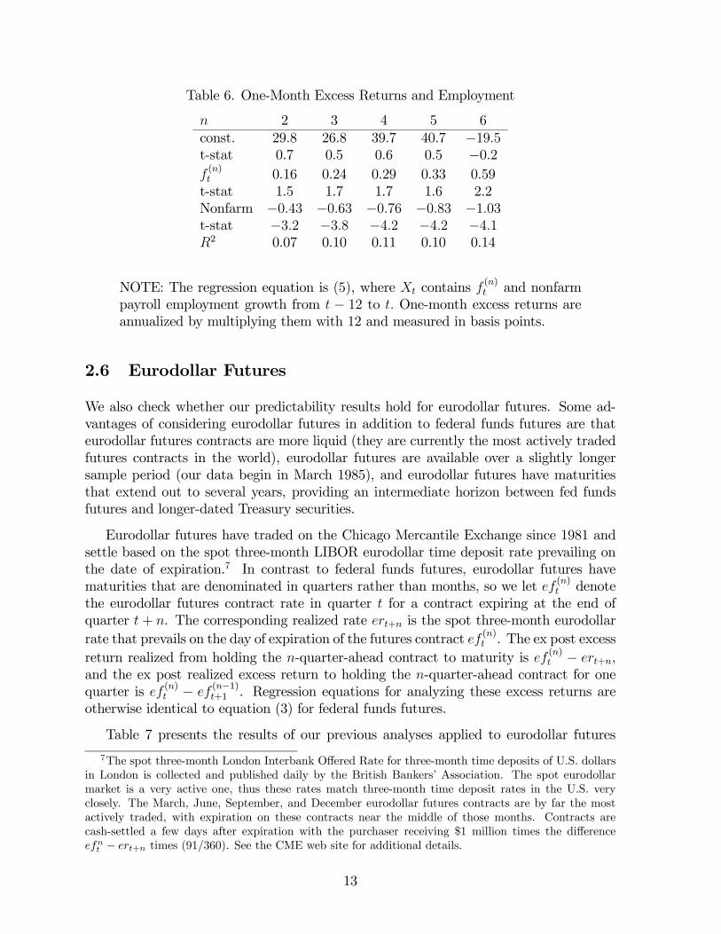
Tables 6 presents the results of our previous analyses applied to this alternative specifi-cation, where the regressors are the own contract rate and employment growth. Althoughthe R2 values are uniformly lower, as is to be expected from quasi-first-differencing theleft-hand side variable, our previous results are robust to this alternative specification.

6The investor’s realized monetary return on this transaction is $5 million times the difference in ratesf(n)t − f

(n−1)t+1 times (number of days in contract month/360). Since these contracts are “marked to

market” essentially every day, the investor realizes the full monetary return to this transaction in montht + 1; in particular, the investor does not need to wait until the contracts mature at the end of montht+ n to realize the return. As before, the opportunity cost of engaging in this transaction is negligible,so the realized return is also the realized excess return.

12

Table 6. One-Month Excess Returns and Employment

n 2 3 4 5 6const. 29.8 26.8 39.7 40.7 −19.5t-stat 0.7 0.5 0.6 0.5 −0.2f(n)t 0.16 0.24 0.29 0.33 0.59t-stat 1.5 1.7 1.7 1.6 2.2Nonfarm −0.43 −0.63 −0.76 −0.83 −1.03t-stat −3.2 −3.8 −4.2 −4.2 −4.1R2 0.07 0.10 0.11 0.10 0.14

NOTE: The regression equation is (5), where Xt contains f(n)t and nonfarm

payroll employment growth from t − 12 to t. One-month excess returns areannualized by multiplying them with 12 and measured in basis points.

2.6 Eurodollar Futures

We also check whether our predictability results hold for eurodollar futures. Some ad-vantages of considering eurodollar futures in addition to federal funds futures are thateurodollar futures contracts are more liquid (they are currently the most actively tradedfutures contracts in the world), eurodollar futures are available over a slightly longersample period (our data begin in March 1985), and eurodollar futures have maturitiesthat extend out to several years, providing an intermediate horizon between fed fundsfutures and longer-dated Treasury securities.

Eurodollar futures have traded on the Chicago Mercantile Exchange since 1981 andsettle based on the spot three-month LIBOR eurodollar time deposit rate prevailing onthe date of expiration.7 In contrast to federal funds futures, eurodollar futures havematurities that are denominated in quarters rather than months, so we let ef (n)t denotethe eurodollar futures contract rate in quarter t for a contract expiring at the end ofquarter t+ n. The corresponding realized rate ert+n is the spot three-month eurodollarrate that prevails on the day of expiration of the futures contract ef (n)t . The ex post excessreturn realized from holding the n-quarter-ahead contract to maturity is ef (n)t − ert+n,and the ex post realized excess return to holding the n-quarter-ahead contract for onequarter is ef (n)t − ef

(n−1)t+1 . Regression equations for analyzing these excess returns are

otherwise identical to equation (3) for federal funds futures.

Table 7 presents the results of our previous analyses applied to eurodollar futures

7The spot three-month London Interbank Offered Rate for three-month time deposits of U.S. dollarsin London is collected and published daily by the British Bankers’ Association. The spot eurodollarmarket is a very active one, thus these rates match three-month time deposit rates in the U.S. veryclosely. The March, June, September, and December eurodollar futures contracts are by far the mostactively traded, with expiration on these contracts near the middle of those months. Contracts arecash-settled a few days after expiration with the purchaser receiving $1 million times the differenceefnt − ert+n times (91/360). See the CME web site for additional details.

13

contracts with maturities of n = 1, . . . , 8 quarters ahead. Panel A shows that averageexcess returns on eurodollar futures are between 60 and 105 basis points per year. Excessreturns also exhibits the same type of predictability pattern as fed funds futures. Panel Bshows that nonfarm payroll employment growth is statistically significant at all horizons,with R2 values ranging from 21 to over 43%. The results for Treasury yield spreads andcorporate bond spreads are also significant and similar to those for fed funds futures (notreported). These results show that if anything, risk premia are even more important foreurodollar futures than what we have estimated for federal funds futures.

Table 7. Results for Eurodollar Futures

Panel A: Average excess returns (annualized)

n 1 2 3 4 5 6 7 8const. 59.9 81.1 70.7 102.5 104.4 102.8 99.1 105.8t-stat 2.5 2.7 2.8 2.8 2.7 2.7 2.7 3.0

Panel B: Predictive regressions using employment growth and futures rate

const. 13.36 −8.9 −14.0 −22.5 −29.1 −26.4 −29.6 −52.4t-stat 0.2 −0.2 −0.4 −0.6 −0.6 −0.5 −0.6 −1.0ef

(n)t 0.32 0.41 0.42 0.42 0.39 0.36 0.33 0.34

t-stat 2.5 4.7 6.4 6.3 5.5 5.0 5.2 5.1NFP −0.84 −0.90 −0.87 −81.8 −0.73 −0.65 −0.55 −0.44t-stat 5.3 −8.3 −11.2 −11.2 −11.6 −10.9 −10.2 −7.6R2 0.21 0.31 0.38 0.42 0.44 0.42 0.39 0.43

3 Predictability of Excess Returns in Real Time

We have documented that excess returns on federal funds futures were predictable bybusiness-cycle indicators such as employment growth, Treasury yield spreads or the cor-porate bond spread. To what extent could an investor have predicted these returns inreal time? To answer this question, we first perform a set of rolling “out-of-sample” re-gressions. To see whether market participants may have based their investment strategieson similar forecasts, we provide some intriguing historical evidence on actual trades inthe fed funds and eurodollar futures market.

3.1 Rolling Regressions

Figure 4 shows real-time forecasts together with full-sample forecasts from Table 2 basedon employment growth and the own futures rate. The real-time forecasts for month t+1are constructed by estimating the slope coefficients with data up to the current month t.

14

1990 1992 1994 1996 1998 2000 2002 2004-200

0

200

400 real-time forecast

full-sample forecast

1990 1992 1994 1996 1998 2000 2002 2004-1

0

1

2

3

4

own futures rate cofficient

1990 1992 1994 1996 1998 2000 2002 2004

-4

-3

-2

-1

0

employment growth coefficient

Figure 4: The top panel shows real-time and full-sample forecasts of rx(4)t+4. The middlepanel shows the rolling estimates of the coefficient on the own futures rate f

(4)t . The

flat line is the full-sample coefficient from Table 2. The lower panel shows the rollingestimates of the coefficient on employment growth. Again, the flat line is the full-samplecoefficient from Table 2.

These forecasts are performed starting in January 1990, when we only have 12 monthsof data to estimate three parameters. The graph suggests that the real-time fitted valuesare quite close to the full-sample fitted values over most of the sample - indeed, the twoseries are essentially identical from the beginning of 1994 onward. The middle and lowerpanels in Figure 4 show the rolling estimates of the slope coefficients together with theirfull sample counterparts. The graphs suggest that the rolling point estimates settle downafter 1994.

3.2 Data on Market Participants’ Long and Short Positions

The previous section shows that excess returns on fed funds and eurodollar futures werepotentially predictable to investors in real time using rolling regressions. In this section,we present some evidence indicating that informed investors at the time actually didcorrectly forecast the excess returns that were subsequently realized.

15

1990 1992 1994 1996 1998 2000 2002 2004-20

-10

0

10

20

30

net positions

1990 1992 1994 1996 1998 2000 2002 20040

10

20

30

40

long positions

short positions

Figure 5: The upper panel shows net positions in eurodollar futures. The lower panelshows long and short positions separately.

The U.S. Commodity Futures Trading Commission (CFTC) requires all individualsor institutions holding 10,000 futures contracts or more in a given commodity to reporttheir positions to the CFTC, and the extent to which these positions are hedged.8 Inthe eurodollar (fed funds) futures markets, about 90% (95%) of open interest is held byindividuals or institutions that must report to the CFTC as a result of this requirement.The CFTC reports the aggregates of these data with a three-day lag, broken down intohedging and non-hedging categories and into short and long positions, in the weeklyCommitments of Traders report, available on the CFTC’s web site.

The lower panel in Figure 5 plots the percentage of long and short open interestin eurodollar futures held by noncommercial market participants–those market partici-pants that are classified by the CFTC as not hedging offsetting positions that arise outof their normal (non-futures related) business operations.9 The number of all open longpositions in these contracts held by noncommercial market participants, expressed as a

8The exact reporting threshold varies by commodity. The 10,000 number applies to eurodollar futures,as reported on the CME’s web site.

9The primary example of a commercial participant in the eurodollar futures market would be afinancial institution engaged in lending to commercial and industrial enterprises for periods of 1 to 5years.

16

percentage of total reportable open interest, is plotted in blue, and the number of allopen short positions (as a percentage of reportable open interest) held by these partici-pants is plotted in red. Analogous data are available for fed funds futures, but we focuson eurodollar futures positions here as this market is thicker, data are available backto 1986, and contracts run off less frequently (only once per quarter rather than everymonth), which reduces some high-frequency variation in the percentage long and shortseries.10 The patterns in federal funds futures noncommercial holdings look very similar,albeit noisier for the reasons cited above.

The patterns that emerge in Figure 5 are striking when compared to the realizedexcess return series plotted earlier. Noncommercial market participants began takingon a huge net long position in late 2000, only a few months before excess returns inthese contracts (both eurodollars and fed funds futures) began to soar. Noncommercialmarket participants also took on substantial net long positions from mid-1990 throughmid-1991 and in late 1995, again correctly forecasting excess returns over these periods,and noncommercial participants took on a very substantial net short position in late 1993through mid-1994, correctly anticipating the strongly negative excess returns that wererealized when the Fed began tightening in 1994.

The upper panel of Figure 5 plots the difference between the noncommercial percent-age long and short series as the “net long position” of noncommercial market participants.Just from eyeballing the figure, we can see that net positions forecast subsequent excessreturns in both the fed funds futures and eurodollar futures markets. Regression analysisconfirms that this variable is highly significant as a predictor of excess returns in the fedfunds futures market at horizons of 3 month or more (and eurodollar futures markets athorizons of 1 quarter or more), with R2 values ranging from 7—19%.

The obvious interpretation of this result is that noncommercial market participantsat the time were well aware of the upcoming excess returns on these contracts andpositioned themselves accordingly, at the expense of those engaged in hedging otherfinancial activities. The hedgers — commercial firms — essentially paid an insurancepremium to noncommercial market participants for providing hedging services. Theserents are not “competed away” by other noncommercial market participants. Thereare several possible answers to this question. The futures market may not be perfectlycompetitive, with barriers to entry and noncommercial market participants facing limitson the size of the positions that they may take; commercial participants with hedgingdemand thus do not face a perfectly elastic supply curve for either the long or short side ofthese futures contracts. Moreover, noncommercial market participants may themselvesbe risk averse. For example, futures traders in these markets may be most averse totaking on risky positions precisely when their own jobs are in jeopardy, around the timesof depressed aggregate economic activity. The hypothesis that excess returns in thesemarkets would be competed away requires both an assumption of perfectly competitivefutures markets and of risk-neutral market participants — both of these assumptions maynot apply.

10Open interest is almost always highest in the front-month or front-quarter contract, so the runningoff of these contracts can create jumps.

17

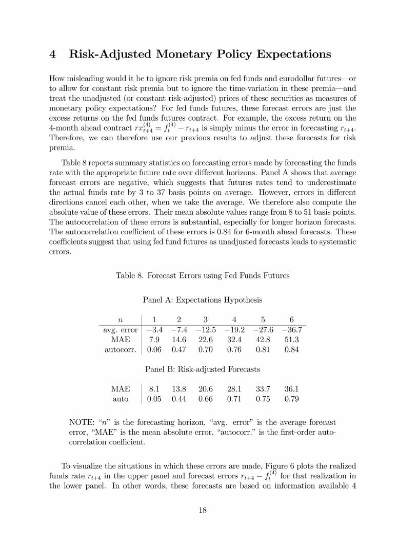
4 Risk-Adjusted Monetary Policy Expectations

How misleading would it be to ignore risk premia on fed funds and eurodollar futures–orto allow for constant risk premia but to ignore the time-variation in these premia–andtreat the unadjusted (or constant risk-adjusted) prices of these securities as measures ofmonetary policy expectations? For fed funds futures, these forecast errors are just theexcess returns on the fed funds futures contract. For example, the excess return on the4-month ahead contract rx(4)t+4 = f

(4)t − rt+4 is simply minus the error in forecasting rt+4.

Therefore, we can therefore use our previous results to adjust these forecasts for riskpremia.

Table 8 reports summary statistics on forecasting errors made by forecasting the fundsrate with the appropriate future rate over different horizons. Panel A shows that averageforecast errors are negative, which suggests that futures rates tend to underestimatethe actual funds rate by 3 to 37 basis points on average. However, errors in differentdirections cancel each other, when we take the average. We therefore also compute theabsolute value of these errors. Their mean absolute values range from 8 to 51 basis points.The autocorrelation of these errors is substantial, especially for longer horizon forecasts.The autocorrelation coefficient of these errors is 0.84 for 6-month ahead forecasts. Thesecoefficients suggest that using fed fund futures as unadjusted forecasts leads to systematicerrors.

Table 8. Forecast Errors using Fed Funds Futures

Panel A: Expectations Hypothesis

n 1 2 3 4 5 6avg. error −3.4 −7.4 −12.5 −19.2 −27.6 −36.7MAE 7.9 14.6 22.6 32.4 42.8 51.3

autocorr. 0.06 0.47 0.70 0.76 0.81 0.84

Panel B: Risk-adjusted Forecasts

MAE 8.1 13.8 20.6 28.1 33.7 36.1auto 0.05 0.44 0.66 0.71 0.75 0.79

NOTE: “n” is the forecasting horizon, “avg. error” is the average forecasterror, “MAE” is the mean absolute error, “autocorr.” is the first-order auto-correlation coefficient.

To visualize the situations in which these errors are made, Figure 6 plots the realizedfunds rate rt+4 in the upper panel and forecast errors rt+4 − f

(4)t for that realization in

the lower panel. In other words, these forecasts are based on information available 4

18

months ago. The forecast errors are already demeaned. Interestingly, Figure 6 suggeststhat forecasts based on the expectations hypothesis tend to adjust to slowly to changesin direction. For example, forecast errors tend to be negative in periods when the fundsrate falls. They tend to be positive in periods when the funds rate goes up. In otherwords, futures rates are useful as an indication of where the funds rate will be in thefuture. However, the indication provided by unadjusted futures rates “lags behind:” longafter the Fed has started easing, the futures rate still forecasts high future funds rates.

We can now use our results from Table 3 to adjust futures-based forecasts for riskpremia. Panel B in Table 8 reports the summary statistics of these forecasts. Since theforecasts are mean zero by construction, we do not report the corresponding rows. Forshort horizons, the absolute errors are comparable to those under the expectations hy-pothesis. For long-horizon forecasts, however, risk-adjusted forecasts are more successfulthan unadjusted forecasts. The difference between the two types of forecasts is 15 ba-sis points. Also, while risk-adjusted forecasts still produce autocorrelated mistakes, theautocorrelation coefficients tend to be smaller than for unadjusted forecasts.

1990 1992 1994 1996 1998 2000 2002 20040

200

400

600

800

1000

actual fed funds rate

1990 1992 1994 1996 1998 2000 2002 2004-150

-100

-50

0

50

100

Figure 6: The upper panel shows the actual funds rate. The lower panel shows forecasterrors with unadjusted (red) and adjusted forecasts (blue).

19

References

[1] Bernanke, Ben and Kenneth Kuttner 2003. “What Explains the Stock Market’sReaction to Federal Reserve Policy?” Forthcoming Journal of Finance.

[2] Brunner, Allan D. 2000. “On the Derivation of Monetary Policy Shocks: ShouldWe Throw out the VAR Out with the Bath Water?” Journal of Money, Credit andBanking 32, 252-79.

[3] Campbell, John Y. and Robert J. Shiller 1991. “Yield Spreads and Interest RateMovements: A Bird’s Eye View.” Review of Economic Studies, 58, 495-514.

[4] Cochrane, John Y. and Monika Piazzesi 2002. “The Fed and Interest Rates: A High-Frequency Identification.”Papers and Proceedings, May 2002, 92, pp. 90-95.

[5] Cochrane, John Y. and Monika Piazzesi 2002. “Bond Risk Premia.” Working paper,University of Chicago.

[6] Durham, Benson 2003. “Estimates of the Term Premium on Near-Dated FederalFunds Futures Contracts.” FEDS Working paper 2003-19, Federal Reserve Board.

[7] Ellingsen and Soderstrom (2003). “Monetary Policy and the Bond Market.” Workingpaper, Bocconi University.

[8] Fama, Eugene F. and Robert R. Bliss 1987. “The Information in Long-MaturityForward Rates.” American Economic Review, 77, 680-692.

[9] Faust, Jon, Eric Swanson and Jonathan Wright 2004. “Identifying VARs Based onHigh-Frequency Futures Data.” Forthcoming Journal of Monetary Economics.

[10] Gurkaynak, Refet, Brian Sack, and Eric Swanson 2002. “Market-based Measuresof Monetary Policy Expectations.” FEDS working paper 2002-40, Federal ReserveBoard.

[11] Gurkaynak, Refet, Brian Sack, and Eric Swanson 2003. “The Excess Sensitivity ofLong-term Interest Rates: Evidence and Implications for Macro Models.” FEDSworking paper 2003-50, Federal Reserve Board.

[12] Hansen, Lars Peter and Robert J. Hodrick, 1988. “Forward Exchange Rates as Opti-mal Predictors of Future Spot Rates: An Econometric Analysis.” Journal of PoliticalEconomy, 88, 829-53.

[13] Hodrick, Robert J., 1992. “Dividend Yields And Expected Stock Returns: Alterna-tive Procedures For Influence And Measurement.” Review of Financial Studies, 5,357-86.

[14] Krueger, Joel T. and Kenneth N. Kuttner 1996. “The Fed Funds Futures Rate as aPredictor of Federal Reserve Policy.” Journal of Futures Markets 16, 865-879.

20

[15] Kuttner, Kenneth N. 2001. “Monetary Policy Surprises and interest rates: Evidencefrom the Federal funds futures market.” Journal of Monetary Economics 47, 523-544.

[16] Lange, Joe, Brian Sack and William Whitesell 2003. “Anticipations of MonetaryPolicy in Financial Markets.” Journal of Money, Credit, and Banking 35, 889-909.

[17] Piazzesi, Monika 2004. “Bond Yields and the Federal Reserve.” Forthcoming Journalof Political Economy.

[18] Rudebusch, Glenn 1998. “Do Measures of Monetary Policy in a VAR Make Sense?”International Economic Review 39, 907-931.

[19] Sack, Brian 2002. “Extracting the Expected Path of Monetary Policy from FuturesRates.” FEDS working paper 2002-56, Federal Reserve Board.

[20] Stigum, Marcia 1990. The Money Market. (New York: McGraw-Hill).

[21] Stock, James H. and Mark W. Watson, 1989. “New Indexes of Coincident andLeading Indicators,” in Olivier Blanchard and Stanley Fischer, Eds., 1989 NBERMacroeconomics Annual, Cambridge MA: MIT Press.

21