Under consideration for publication in Theory and Practice of Logic Programming 1

Fuzzy Answer Sets Approximations

MARIO ALVIANO∗Department of Mathematics and Computer Science, University of Calabria, 87036 Rende (CS), Italy

(e-mail: alviano@mat.unical.it)

RAFAEL PENALOZA†Dresden University of Technology, 01062 Dresden, Germany

Center for Advancing Electronics Dresden(e-mail: penaloza@tcs.inf.tu-dresden.de)

submitted 10 April 2013; revised 23 May 2013; accepted 23 June 2013

Abstract

Fuzzy answer set programming (FASP) is a recent formalism for knowledge representation thatenriches the declarativity of answer set programming by allowing propositions to be graded.To now, no implementations of FASP solvers are available and all current proposals are basedon compilations of logic programs into different paradigms, like mixed integer programs orbilevel programs. These approaches introduce many auxiliary variables which might affect theperformance of a solver negatively. To limit this downside, operators for approximating fuzzyanswer sets can be introduced: Given a FASP program, these operators compute lower andupper bounds for all atoms in the program such that all answer sets are between these bounds.This paper analyzes several operators of this kind which are based on linear programming,fuzzy unfounded sets and source pointers. Furthermore, the paper reports on a prototypicalimplementation, also describing strategies for avoiding computations of these operators whenthey are guaranteed to not improve current bounds. The operators and their implementationcan be used to obtain more constrained mixed integer or bilevel programs, or even for providinga basis for implementing a native FASP solver. Interestingly, the semantics of relevant classes ofprograms with unique answer sets, like positive programs and programs with stratified negation,can be already computed by the prototype without the need for an external tool.

KEYWORDS: Fuzzy logic, answer set programming, search-space pruning operators

1 Introduction

Answer Set Programming (ASP), i.e., logic programming under stable model seman-

tics (Gelfond and Lifschitz 1991), is a declarative language for knowledge representation

(Niemela 1999; Marek and Truszczynski 1999; Lifschitz 2002). In ASP, problems are

modeled by specifying a set of requirements that all solutions, called answer sets, have to

satisfy. One of the strengths of ASP is its capability to model non-monotonic knowledge,

overcoming a well-known limitation of classical logic, which can only deal with mono-

tonic inferences. While monotonicity is desired in mathematics, it is widely considered

a weakness for knowledge representation (Baral 2003), where non-monotonicity arises in

∗ Partially supported by Regione Calabria within the PIA project KnowRex POR FESR 2007–2013.† Partially supported by DFG under grant BA 1122/17-1 and within the Cluster of Excellence ‘cfAED’.

2 M. Alviano and R. Penaloza

common reasoning tasks such as reasoning by default, abductive reasoning and belief

revision. ASP can handle these tasks naturally (Marek and Remmel 2004; Lin and You

2002; Delgrande et al. 2008), allowing for modeling and reasoning on incomplete infor-

mation, and possibly retracting some conclusions as new knowledge on the application

domain is acquired. Since complete knowledge can only be achieved in mathematical

abstraction, it can be stated that ASP makes logic closer to the real world.

However, ASP is still based on precise information, which cannot always be assumed

in the real world. For example, measures provided by any instrument or sensor always

come with some degree of tolerance, and information expressed in natural language are

often vague: there is no precise way to distinguish persons that are tall from those who

are not. Fuzzy logic (Dubois et al. 1991) can handle vague information of this kind

by interpreting propositions with a truth degree in the interval of real numbers [0, 1].

Intuitively, the higher the degree assigned to a proposition, the more true it is, with the

extreme elements 0 and 1 denoting totally false and totally true, respectively. Consider for

example the Barber of Seville paradox: In the small town of Seville, all and only those

men who do not shave themselves are shaved by the barber. Classical set theory can

neither prove nor disprove that the barber shaves himself, hence a fuzzy interpretation

of this proposition should be 1/2, the most undetermined truth degree.

Fuzzy Answer Set Programming (FASP) aims at combining ASP and fuzzy logic. For

example, a FASP encoding of the Barber of Seville paradox is

shaves(barber,X )← not shaves(X ,X ) shaves(X ,X )← not shaves(barber,X )

from which shaves(barber, barber) gets the expected truth degree 1/2. FASP has been

defined for a very general framework (Nieuwenborgh et al. 2007b), allowing several con-

nectors to be combined in the same program. With the aim of providing an indication

for implementing a FASP solver, more constrained frameworks have been considered by

Lukasiewicz (2006) and Janssen et al. (2012). However, current proposals are based on

compilations into different paradigms and introduce many auxiliary variables which could

affect performance negatively. The focus of this paper is on operators for approximating

fuzzy answer sets. These operators can be used for limiting the search space of an exter-

nal tool, such as the linear or bilevel program approaches proposed by Lukasiewicz and

Janssen et al., or as the basis for implementing a native FASP solver.

More precisely, in this paper we describe operators for computing two fuzzy interpreta-

tions, called lower and upper bound, such that every answer set is between these bounds.

We introduce fuzzy unfounded sets, which generalize the notion of unfounded sets of

classical ASP to deal with fuzzy semantics. We also define a well-founded operator that

combines the fuzzy TP operator with the complement of the greatest unfounded set to

improve on previously computed bounds. We show that these operators yield answer sets

for positive and stratified FASP programs in polynomial time, while in general produce

the well-founded semantics by Damasio and Pereira (2001). For dealing with normal

FASP programs, we introduce the new minimal satisfiability operator SP . For semantics

based on the Lukasiewicz t-norm, this operator is polynomial-time computable and can

further tighten the approximation. Finally, we describe a prototypical implementation

which combines optimization ideas from classical ASP solvers (Gebser et al. 2007; Lier-

ler and Maratea 2004; Alviano et al. 2011), and report on an experiment assessing the

potential performance gain provided by our operators to a bilevel program solver.

Fuzzy Answer Sets Approximations 3

2 Syntax and Semantics

Let B be a fixed, finite set of propositional atoms. A fuzzy atom (or atom for short)

is either a propositional atom from B or a numeric constant in the range [0, 1], where

numeric constants are overlined, e.g. 1, to distinguish them from propositional atoms. A

literal is either a fuzzy atom or a fuzzy atom preceded by the default negation symbol

not. A normal FASP program is a finite set of rules of the form

a ← b1 ⊗ · · · ⊗ bm ⊗ not bm+1 ⊗ · · · ⊗ not bn (1)

where n ≥ m ≥ 0, a, b1, . . . , bn are atoms, and ⊗ denotes the fuzzy conjunction. For

a rule r of the form (1), the atom a is called the head of r , denoted H (r), and the

conjunction b1 ⊗ · · · ⊗ bm ⊗ not bm+1 ⊗ · · · ⊗ not bn is called the body of r , denoted

B(r). The expressions B+(r) = b1, . . . , bm and B−(r) = bm+1, . . . , bn denote the

multiset of positive and negative body literals of r , respectively. Multisets thus represent

conjunctions: a multiset A = a1, . . . , ak (k ≥ 0) of literals represents the conjunction⊗ki=1 ai . Moreover, not A denotes the multiset not a1, . . . , not ak, i.e.,

⊗ki=1 not ai . A

rule r is positive if B−(r) = ∅, and a fact if B+(r) = B−(r) = ∅. Relevant subclasses of

normal FASP programs are the positive and stratified programs. A program is positive

if all of its rules are positive. The notion of stratified program requires the introduction

of the dependency graph GP = (B,A) of a program P , where A contains arcs a →+ biand a →− bj (1 ≤ i ≤ m < j ≤ n) for each rule r ∈ P of the form (1). P is stratified if

no cycle in GP contains →− arcs.

The semantics of FASP programs generalizes that of ASP by interpreting propositional

atoms with a truth degree from the interval [0, 1]. An additional degree of liberty arises

from the choice of the operator used to interpret fuzzy conjunctions. We focus on se-

mantics based on t-norms (Klement et al. 2000). A t-norm is a binary, associative and

commutative operator ⊗ : [0, 1] × [0, 1] → [0, 1] that is monotonic and has unit 1, i.e.,

for every x , y , z ∈ [0, 1], x ≤ y implies x ⊗ z ≤ y ⊗ z , and x ⊗ 1 = x . There are three

fundamental t-norms, called the Godel, Lukasiewicz, and product t-norms, where x ⊗ y

is defined as minx , y, maxx + y − 1, 0, and x · y , respectively. In the following, FASP

programs are assumed to be associated with a fixed t-norm computable in polynomial

time. A fuzzy interpretation I for a FASP program P is a fuzzy set in B, i.e., a function

I : B → [0, 1] mapping each propositional atom of B into a truth degree in [0, 1]. The

interpretation I is extended to numeric constants, negative literals and multisets as fol-

lows. For a constant c, I (c) = c; for a negative literal not b, I (not b) = 1 − I (b); for a

multiset of literals A = l1, · · · , lk, I (A) =⊗k

i=1 I (li).

Let I be the set of all interpretations and I , J ∈ I. I is a subset of J (I ⊆ J ) if

I (a) ≤ J (a) for each a ∈ B. I is a strict subset of J (I ⊂ J ) if I ⊆ J and I 6= J .

Fuzzy set intersection (I ∩J ), union (I ∪J ), and difference (I \J ) are defined as follows:

for every a ∈ B, [I ∩ J ](a) := minI (a), J (a), [I ∪ J ](a) := maxI (a), J (a), and

[I \ J ](a) := maxI (a) − J (a), 0. An interpretation I models a rule r with head a,

denoted I |= r , if I (a) ≥ I (B(r)). I models a FASP program P (I |= P) if I |= r for

each r ∈ P . An interpretation M is an answer set of a positive FASP program P if M is a

minimal model of P , i.e., M |= P and there is no interpretation I ⊂ M such that I |= P .

M is an answer set of a normal FASP program P if M is an answer set of the reduct PM

obtained from P by replacing each negative literal not b by the constant I (not b).

4 M. Alviano and R. Penaloza

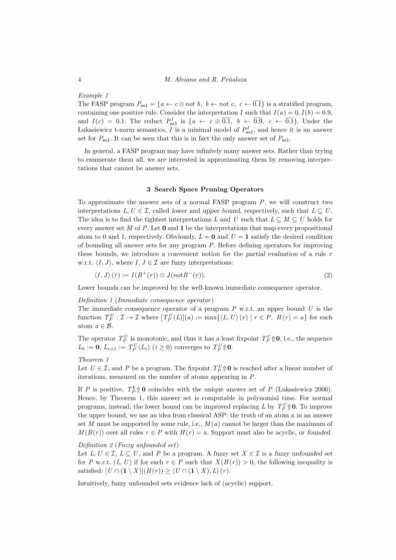
Example 1

The FASP program Pex1 = a ← c⊗not b, b ← not c, c ← 0.1 is a stratified program,

containing one positive rule. Consider the interpretation I such that I (a) = 0, I (b) = 0.9,

and I (c) = 0.1. The reduct P Iex1 is a ← c ⊗ 0.1, b ← 0.9, c ← 0.1. Under the

Lukasiewicz t-norm semantics, I is a minimal model of P Iex1, and hence it is an answer

set for Pex1. It can be seen that this is in fact the only answer set of Pex1.

In general, a FASP program may have infinitely many answer sets. Rather than trying

to enumerate them all, we are interested in approximating them by removing interpre-

tations that cannot be answer sets.

3 Search Space Pruning Operators

To approximate the answer sets of a normal FASP program P , we will construct two

interpretations L,U ∈ I, called lower and upper bound, respectively, such that L ⊆ U .

The idea is to find the tightest interpretations L and U such that L ⊆ M ⊆ U holds for

every answer set M of P . Let 0 and 1 be the interpretations that map every propositional

atom to 0 and 1, respectively. Obviously, L = 0 and U = 1 satisfy the desired condition

of bounding all answer sets for any program P . Before defining operators for improving

these bounds, we introduce a convenient notion for the partial evaluation of a rule r

w.r.t. 〈I , J 〉, where I , J ∈ I are fuzzy interpretations:

〈I , J 〉 (r) := I (B+(r))⊗ J (notB−(r)). (2)

Lower bounds can be improved by the well-known immediate consequence operator.

Definition 1 (Immediate consequence operator)

The immediate consequence operator of a program P w.r.t. an upper bound U is the

function TUP : I → I where [TU

P (L)](a) := max〈L,U 〉 (r) | r ∈ P , H (r) = a for each

atom a ∈ B.

The operator TUP is monotonic, and thus it has a least fixpoint TU

P ⇑0, i.e., the sequence

L0 := 0, Li+1 := TUP (Li) (i ≥ 0) converges to TU

P ⇑0.

Theorem 1

Let U ∈ I, and P be a program. The fixpoint TUP ⇑0 is reached after a linear number of

iterations, measured on the number of atoms appearing in P .

If P is positive, T1P⇑ 0 coincides with the unique answer set of P (Lukasiewicz 2006).

Hence, by Theorem 1, this answer set is computable in polynomial time. For normal

programs, instead, the lower bound can be improved replacing L by TUP ⇑0. To improve

the upper bound, we use an idea from classical ASP: the truth of an atom a in an answer

set M must be supported by some rule, i.e., M (a) cannot be larger than the maximum of

M (B(r)) over all rules r ∈ P with H (r) = a. Support must also be acyclic, or founded.

Definition 2 (Fuzzy unfounded set)

Let L,U ∈ I, L ⊆ U , and P be a program. A fuzzy set X ∈ I is a fuzzy unfounded set

for P w.r.t. (L,U ) if for each r ∈ P such that X (H (r)) > 0, the following inequality is

satisfied: [U ∩ (1 \X )](H (r)) ≥ 〈U ∩ (1 \X ),L〉 (r).

Intuitively, fuzzy unfounded sets evidence lack of (acyclic) support.

Fuzzy Answer Sets Approximations 5

Theorem 2For FASP programs without numeric constants and crisp sets, Definition 2 coincides with

the original notion of unfounded set by Van Gelder et al. (1991).

As in the crisp case, the union of two (fuzzy) unfounded sets is an unfounded set.

Theorem 3Let X1,X2 be two fuzzy unfounded sets for P w.r.t. (L,U ). Then also X1 ∪X2 is a fuzzy

unfounded set for P w.r.t. (L,U ).

We can thus define the greatest fuzzy unfounded set, denoted GUSL,UP , as the union of

all fuzzy unfounded sets. We also highlight a relationship with fuzzy answer sets.

Theorem 4M is a fuzzy answer set of a program P if and only if GUSM ,M

P = 1 \M .

In order to find unfounded sets, we can employ the operator RP , defined next.

Definition 3 (Operator RP )Let L,U ∈ I. The operator RP for a program P w.r.t. (L,U ) is the function RL,U

P : I → Isuch that [RL,U

P (X )](a) := minX (a), 1−max〈U ∩ (1 \X ),L〉 (r) | r ∈ P , H (r) = afor every a ∈ B.

The operator RL,UP is antitonic; thus it has a greatest fixpoint RL,U

P ⇓ 1, which is the

limit of the sequence X0 := 1, Xi+1 := RL,UP (Xi), i ≥ 0. There is a strong relationship

between fuzzy unfounded sets and the operator RP , which allows for replacing the upper

bound U by 1 \ (RL,UP ⇓1).

Theorem 5Let L,U ∈ I, L ⊆ U , and P be a program. If 1\RL,U

P ⇓1 ⊆ U , then RL,UP ⇓1 = GUSL,U

P .

It is easy to see that one application of the RP operator requires linear time in the

number of rules P . Moreover, as in Theorem 1, the greatest fixpoint RL,UP ⇓1 is obtained

after at most as many applications of this operator as there are atoms in P . In total, this

means that this fixpoint can be computed in polynomial time on the size of P .

Theorem 6Let L,U ∈ I and P be a program. The fixpoint RL,U

P ⇓1 can be computed in polynomial

time on the size of P .

To sum up, the TP operator can be used to improve the lower bound L, while RP is

useful for decreasing the upper bound U . These two operators complement each other,

as a tighter lower bound may help to further decrease the upper bound, and dually, a

tighter upper bound may increase the lower bound. In fact, if L ⊆ L′ and U ′ ⊆ U , then

(i) TUP (I ) ⊆ TU ′

P (I ) and (ii) RL′,UP (I ) ⊆ RL,U

P (I ), thus 1 \RL,UP (I ) ⊆ 1 \RL′,U

P (I ) hold

for every interpretation I . We can then combine TP and RP to obtain a new operator.

Definition 4 (Well-founded operator)The well-founded operator is the function WP : I × I → I × I defined as

WP (L,U ) :=(

TUP (L),1 \ RL,U

P ⇓1)

. (3)

The well-founded operator is monotonic in the lattice (I×I,≤), where (L,U ) ≤ (L′,U ′)

if and only if L ⊆ L′ and U ′ ⊆ U . Hence, WP has a least fixpoint WP⇑(0,1). Moreover,

every pair Wi = (Li ,Ui) in the sequence W0 := (0,1), Wi+1 := WP (Wi) (i ≥ 0) satisfies

that Li ⊆ M ⊆ Ui for every answer set M of P . We show a stronger result.

6 M. Alviano and R. Penaloza

Theorem 7Let P be a program, L,U two interpretations, (L′,U ′) = WP (L,U ), and M an answer

set for P . If L ⊆ M ⊆ U , then L′ ⊆ M ⊆ U ′.

Just as TP does for positive programs, an iterative application of the well-founded oper-

ator yields the unique answer set of stratified programs in polynomial time.

Theorem 8Let P be a stratified program. The least fixpoint of WP coincides with the unique answer

set of P and is computable in polynomial time.

Example 2Consider the stratified program Pex1 from Example 1. The application of the well-founded

operator to Pex1 are shown in Table 1. After three iterations, a fixpoint is reached,

stating that every answer set M for Pex1 must be such that M (a) = 0, M (b) = 0.9, and

M (c) = 0.1. As seen before, this is indeed the only answer set of Pex1.

Although it is only possible to guarantee that the iterative application of the combined

operator computes an answer set if the program is stratified, they can also produce the

answer sets of cyclic programs, as shown by the following example.

Example 3For the program Pex2 = Pex1 ∪ b ← not a, Table 1 shows the applications of WP . A

fixpoint is reached after four iterations, stating that the only candidate for an answer

set is the interpretation M with M (a) = 0, M (b) = 1, and M (c) = 0.1. The reduct of

Pex2 w.r.t. M is a ← c ⊗ 0, b ← 0.9, c ← 0.1, b ← 1, for which M is a minimal

model. However, the iterative application of WP might not terminate, as for example for

program Pinf = a ← 0.9 ⊗ not a over the product t-norm. The least fixpoint of WPinf

assigns to a degree 9/19, but ω applications are required.

Even if WP often provides good bounds, there is still room for improvement. Consider

the program Podd = a ← not a. Podd has exactly one answer set M with M (a) = 1/2.

However, WP yields the bounds L = 0 and U = 1. Observe that the rule of Podd states

the implicit restriction that a must be evaluated to at least 1/2 in every model I of P

because I |= P implies I (a) ≥ I (not a) = 1 − I (a). Implicit restrictions of this kind

might be used to further improve lower bounds.

Definition 5 (Minimal satisfiability)The minimal satisfiability operator of a program P w.r.t. an upper bound U is the

function SUP : I → I where [SU

P (L)](a) := infI (a) | I |= P ,L ⊆ I ⊆ U for each a ∈ B.

Table 1. Iterations of the combined operator on Pex1 and Pex2

Pex1 Pex2

a b c a b c

L0 := 0 ;U0 := 1 0; 1 0 ; 1 0 ; 1 0 ; 1 0 ; 1 0 ; 1

L1 := TU0P (L0);U1 := 1 \ RL0,U0

P ⇓1 0; 0.1 0 ; 1 0.1; 0.1 0 ; 0.1 0 ; 1 0.1; 0.1

L2 := TU1P (L1);U2 := 1 \ RL1,U1

P ⇓1 0; 0.1 0.9; 0.9 0.1; 0.1 0 ; 0.1 0.9; 1 0.1; 0.1

L3 := TU2P (L2);U3 := 1 \ RL2,U2

P ⇓1 0; 0 0.9; 0.9 0.1; 0.1 0 ; 0 0.9; 1 0.1; 0.1

L4 := TU3P (L3);U4 := 1 \ RL3,U3

P ⇓1 0; 0 0.9; 0.9 0.1; 0.1 0 ; 0 1 ; 1 0.1; 0.1

L5 := TU4P (L4);U5 := 1 \ RL4,U4

P ⇓1 0; 0 0.9; 0.9 0.1; 0.1 0 ; 0 1 ; 1 0.1; 0.1

Fuzzy Answer Sets Approximations 7

Theorem 9

Let L,U ,M ∈ I and P be a program. If M |= P and L ⊆ M ⊆ U , then SUP (L) ⊆ M ⊆ U .

It is thus possible to improve the bounds by an iterative application of the SP and RP

operators. It is also easy to see that TUP (L) ⊆ SU

P (L). This in particular means that the

lower bound obtained by SP is always at least as good as the one given by TP , and in

some cases strictly better. This translates not only in better bounds being computed,

but also in a lower number of iterations needed to obtain them. Unfortunately, in general

it is not clear how to compute the minimal satisfiability operator, as it requires finding

optimal values for a possibly complex system of constraints, depending on the t-norm.

If we restrict to the Lukasiewicz t-norm, then SP reduces to solving a series of linear

programming problems. More precisely, for a program P we define a finite system of

inequalities LP having, for each rule r ∈ P of the form (1), one inequality

a ≥ b1 + . . .+ bm − bm+1 − . . .− bn + 1−m (4)

such that all variables a, b1, . . . , bn are restricted to the interval [0, 1]. All models of P

must satisfy LP and vice versa. Thus, we obtain the following result.

Theorem 10

Let P be a program over the Lukasiewicz t-norm, and L,U ∈ I. For every atom a ∈ Bit holds that [SU

P (L)](a) = minI (a) | I satisfies LP ∪ L(b) ≤ I (b) ≤ U (b) | b ∈ B.

In this case, the minimal satisfiability operator can be computed efficiently.

Theorem 11

Let L,U ∈ I, and P be a program over the Lukasiewicz t-norm. SUP (L) is computable

in polynomial time w.r.t. the number of rules.

Consider again program Podd . SP computes the minimal value for a with a ≥ 1− a, i.e.,

1/2. The lower bound is updated to 1/2. Then, RP yields RP (L) = 1/2, and updates the

upper bound to 1/2. Further applications of the operators do not modify L or U , hence

M (a) = 1/2 is our candidate answer set, which in this case is the correct solution.

4 Implementation and Experiment

We developed fasp, a prototype handling propositional FASP programs. Programs with

variables can be transformed into equivalent propositional FASP programs by means of an

almost standard grounding procedure, for example by using gringo (Gebser et al. 2007),

which we extended to deal with numeric constants. The prototype is available at https:

//github.com/alviano/fasp.git. In the input program, numeric constants are speci-

fied by writing a decimal or fractional number preceded by a # character. The output of

gringo is a numeric format which constitutes the input of fasp. The output of fasp is the

fuzzy answer sets approximation obtained by the operators described in Section 3 w.r.t.

the t-norm specified by the command-line option --tnorm=TNORM, where the currently im-

plemented TNORMs are lukasiewicz (default), godel, and product. For the Lukasiewicz

t-norm, fasp can also produce the bilevel program defined by Blondeel et al. (2012),

which is encoded for the library YALMIP (http://users.isy.liu.se/johanl/yalmip)

and can be solved by invoking octave (http://www.gnu.org/software/octave/). The

8 M. Alviano and R. Penaloza

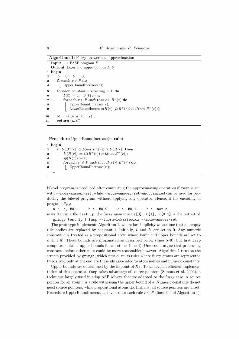
Algorithm 1: Fuzzy answer sets approximation

Input : a FASP program POutput: lower and upper bounds L,U

1 begin2 L := 0; U := 0;3 foreach r ∈ P do4 UpperBoundIncrease(r);

5 foreach constant c occurring in P do6 L(c) := c; U (c) := c;7 foreach r ∈ P such that c ∈ B+(r) do8 UpperBoundIncrease(r);9 LowerBoundIncrease(H (r), L(B+(r))⊗U (not B−(r)));

10 MinimalSatisfiability();11 return (L,U )

Procedure UpperBoundIncrease(r : rule)

1 begin2 if U (B+(r))⊗ L(not B−(r)) > U (H (r)) then3 U (H (r)) := U (B+(r))⊗ L(not B−(r));4 sp(H (r)) := r ;5 foreach r ′ ∈ P such that H (r) ∈ B+(r ′) do6 UpperBoundIncrease(r ′);

bilevel program is produced after computing the approximating operators if fasp is run

with --mode=answer-set, while --mode=answer-set-unoptimized can be used for pro-

ducing the bilevel program without applying any operator. Hence, if the encoding of

program Pex2:

a :- c, #0.1. b :- #0.9. c :- #0.1. b :- not a.

is written in a file test.lp, the fuzzy answer set a[0], b[1], c[0.1] is the output of

gringo test.lp | fasp --tnorm=lukasiewicz --mode=answer-set

The prototype implements Algorithm 1, where for simplicity we assume that all empty

rule bodies are replaced by constant 1. Initially, L and U are set to 0. Any numeric

constant c is treated as a propositional atom whose lower and upper bounds are set to

c (line 6). These bounds are propagated as described below (lines 5–9), but first fasp

computes suitable upper bounds for all atoms (line 4). One could argue that processing

constants before other rules could be more reasonable; however, Algorithm 1 runs on the

stream provided by gringo, which first outputs rules where fuzzy atoms are represented

by ids, and only at the end are these ids associated to atom names and numeric constants.

Upper bounds are determined by the fixpoint of RP . To achieve an efficient implemen-

tation of this operator, fasp takes advantage of source pointers (Simons et al. 2002), a

technique largely used in crisp ASP solvers that we adapted to the fuzzy case. A source

pointer for an atom a is a rule witnessing the upper bound of a. Numeric constants do not

need source pointers, while propositional atoms do. Initially, all source pointers are unset.

Procedure UpperBoundIncrease is invoked for each rule r ∈ P (lines 3–4 of Algorithm 1).

Fuzzy Answer Sets Approximations 9

Procedure LowerBoundIncrease(a: atom, d : degree)

1 begin2 if d > L(a) then3 L(a) := d ;4 foreach r ∈ P such that a ∈ B+(r) do5 LowerBoundIncrease(H (r), L(B+(r))⊗U (not B−(r)));

6 foreach r ∈ P such that a ∈ B−(r) do7 UpperBoundDecrease(r);

Procedure UpperBoundDecrease(r : rule)

1 begin2 if sp(H (r)) = r and U (H (r))−U (B+(r))⊗ L(not B−(r)) > ε then3 U (H (r)) := U (B+(r))⊗ L(not B−(r));4 foreach r ′ ∈ P such that H (r) ∈ B+(r ′) do5 UpperBoundDecrease(r ′);

6 foreach r ′ ∈ P such that H (r) ∈ B−(r ′) do7 LowerBoundIncrease(H (r ′), L(B+(r ′))⊗U (not B−(r ′)));

8 r ′ := arg minr′′∈P U (B+(r ′′))⊗ L(not B−(r ′′));9 UpperBoundIncrease(r ′);

The procedure computes the upper bound for B(r) as d = U (B+(r))⊗L(not B−(r)). If

d is strictly greater than U (H (r)), the upper bound of H (r) is set to d and the source

pointer of H (r) is set to r (lines 2–4). This new upper bound for H (r) is propagated

in each rule r ′ in which H (r) occurs as a positive body literal (lines 5–6), possibly in-

creasing the upper bound of H (r ′) and changing its source pointer to r ′. At the end

of this process, atoms having upper bound different from 0 have source pointers set.

Lower bounds, instead, are given by the fixpoint of TP , obtained by first processing facts

and then numeric constants. Each new lower bound d , say for atom a, can increase the

lower bound of the head atom of any rule r in which a occurs as a positive body literal

(lines 2–5 of LowerBoundIncrease). More specifically, H (r) has a new lower bound set to

L(B+(r))⊗U (not B−(r)) if this degree is strictly greater than L(H (r)).

Lower and upper bound updates can interact intensively to obtain better bounds, and

our system handles these interactions as soon as possible. Whenever the lower bound of

an atom a is increased, the system checks whether decreasing the upper bound of the

head atom of any rule r in which a occurs as a negative literal is possible (lines 6–7 of

LowerBoundIncrease). In particular, this might happen if r is the source pointer of H (r),

in which case the upper bound of H (r) might be decreased to U (B+(r))⊗L(not B−(r)).

(To ensure termination, the upper bound is updated only if the decrease is greater than a

fixed constant ε.) This propagation is handled by procedure UpperBoundDecrease, which

first checks whether other upper bounds have to be decreased (lines 4–5). To this end,

only rules in which H (r) occurs as a positive body literal have to be checked, and source

pointers allow to skip most of these rules. Once upper bounds have been decreased, the

procedure possibly increases the lower bounds of the head atom of any rule r ′ in which

10 M. Alviano and R. Penaloza

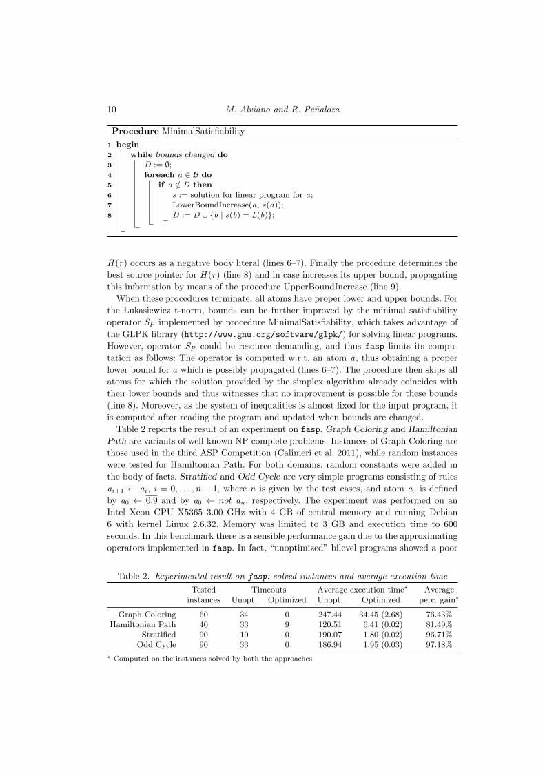
Procedure MinimalSatisfiability

1 begin2 while bounds changed do3 D := ∅;4 foreach a ∈ B do5 if a /∈ D then6 s := solution for linear program for a;7 LowerBoundIncrease(a, s(a));8 D := D ∪ b | s(b) = L(b);

H (r) occurs as a negative body literal (lines 6–7). Finally the procedure determines the

best source pointer for H (r) (line 8) and in case increases its upper bound, propagating

this information by means of the procedure UpperBoundIncrease (line 9).

When these procedures terminate, all atoms have proper lower and upper bounds. For

the Lukasiewicz t-norm, bounds can be further improved by the minimal satisfiability

operator SP implemented by procedure MinimalSatisfiability, which takes advantage of

the GLPK library (http://www.gnu.org/software/glpk/) for solving linear programs.

However, operator SP could be resource demanding, and thus fasp limits its compu-

tation as follows: The operator is computed w.r.t. an atom a, thus obtaining a proper

lower bound for a which is possibly propagated (lines 6–7). The procedure then skips all

atoms for which the solution provided by the simplex algorithm already coincides with

their lower bounds and thus witnesses that no improvement is possible for these bounds

(line 8). Moreover, as the system of inequalities is almost fixed for the input program, it

is computed after reading the program and updated when bounds are changed.

Table 2 reports the result of an experiment on fasp. Graph Coloring and Hamiltonian

Path are variants of well-known NP-complete problems. Instances of Graph Coloring are

those used in the third ASP Competition (Calimeri et al. 2011), while random instances

were tested for Hamiltonian Path. For both domains, random constants were added in

the body of facts. Stratified and Odd Cycle are very simple programs consisting of rules

ai+1 ← ai , i = 0, . . . ,n − 1, where n is given by the test cases, and atom a0 is defined

by a0 ← 0.9 and by a0 ← not an , respectively. The experiment was performed on an

Intel Xeon CPU X5365 3.00 GHz with 4 GB of central memory and running Debian

6 with kernel Linux 2.6.32. Memory was limited to 3 GB and execution time to 600

seconds. In this benchmark there is a sensible performance gain due to the approximating

operators implemented in fasp. In fact, “unoptimized” bilevel programs showed a poor

Table 2. Experimental result on fasp: solved instances and average execution time

Tested Timeouts Average execution time? Averageinstances Unopt. Optimized Unopt. Optimized perc. gain?

Graph Coloring 60 34 0 247.44 34.45 (2.68) 76.43%Hamiltonian Path 40 33 9 120.51 6.41 (0.02) 81.49%

Stratified 90 10 0 190.07 1.80 (0.02) 96.71%Odd Cycle 90 33 0 186.94 1.95 (0.03) 97.18%

? Computed on the instances solved by both the approaches.

Fuzzy Answer Sets Approximations 11

performance, timing out 110 times, while the “optimizied” approach timed out only 9

times (on which also the “unoptimized” approach timed out). Even restricting to the

170 test cases solved by the unoptimized apprach, there is a significant advantage of the

optimized approach, evidenced by an average percentage gain of at least 76%. Note that

in Table 2 the time required for computing the approximation operators is reported in

parentheses and included in the execution time of the optimized approach.

5 Related Work

The study of fuzzy extensions of logic programs can be traced back more than two

decades (see e.g. Dubois et al. 1991). Moreover, compared to classical logic, fuzzy logics

offer several additional levels of liberty for the definition of their semantics; namely, the

choice of the space of truth degrees, the interpretation of the conjunction, the negation,

and even the implication. Hence, we describe only the work that is closest related to ours.

The first generalization of the immediate consequence operator to deal with fuzzy

semantics was due to Achs and Kiss (1995) and Achs (1997), albeit exclusively for the

Godel t-norm semantics. Fuzzy answer set semantics were introduced by Lukasiewicz

(2006) based on a generalization of the Gelfond-Lifschitz transformation (Damasio and

Pereira 2001). It was then shown that positive and stratified programs have a unique

answer set, and that it can be obtained by a finite iteration of the TP operator. However,

no further analysis on the number of iterations needed to obtain that answer set was

made. It is worth noting that the semantics described by Lukasiewicz are based on a finite

set of truth values, rather than the whole interval [0, 1], as in our case. Nonetheless, the

proof ideas can be generalized to arbitrary t-norms over [0, 1] without difficulty. General

fuzzy answer set programs have been studied in detail in the last years (Janssen 2011),

considering not only general t-norm semantics, but also arbitrary connectives to be used

in the head and the body of the rules.

While the complexity of finding fuzzy answer sets is now relatively well understood,

there were to-date no solvers available. In an effort to compute answer sets for general

programs, a completion method was proposed by Janssen et al. (2012). The idea is to

transform the program P into a set of fuzzy logic formulas, whose models correspond

precisely to the answer sets of P . However, due to the lack of (optimized) fuzzy logic

reasoners, this reduction does not allow for an effective implementation. A different ap-

proach, specifically designed for the Lukasiewicz t-norm, is to reduce the program P to

a bilevel linear programming problem (Blondeel et al. 2012). This method, which is also

implemented by our system, has important theoretical repercussions, e.g., it can be used

to show that disjunctions on rule heads do not add expressivity under this semantics.

Unfounded sets for FASP programs were first defined by Nieuwenborgh et al. (2007a);

these unfounded sets are defined w.r.t. total interpretations and are actually crisp sets

used for characterizing fuzzy answer sets. We will refer to this notion as crisp unfounded

sets. Our definition is more general: it is given w.r.t. partial interpretations and for fuzzy

sets; it is suitable for pruning the search space but also characterizes answer sets. A

relationship between the two notions follows by Theorem 4.

Corollary 1

For every fuzzy unfounded set X w.r.t. (I , I ), set a | X (a) + I (a) > 1 is a crisp

12 M. Alviano and R. Penaloza

unfounded set. For every crisp unfounded set Y there is a fuzzy unfounded set X such

that Y = a | X (a) + I (a) > 1.

To the best of our knowledge, there had been no previous attempts to generalize the

RP operator as a complementation of unfounded sets. This operator allows for a better

approximation of answer sets without spending too many resources. A similar idea was

studied by Loyer and Straccia (2009), where a well-founded semantics is used for querying

fuzzy logic programs over the Godel t-norm. A well-founded semantics was also defined

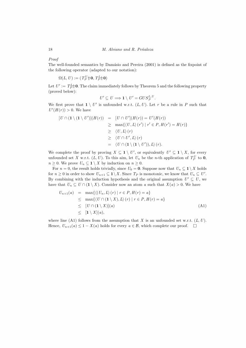
by Damasio and Pereira (2001), for which we can prove the following result.

Theorem 12

The fixpoint of WP gives the well-founded semantics by Damasio and Pereira (2001).

6 Conclusions

We studied the problem of finding answer sets for normal FASP programs with t-norm

based semantics. We studied fuzzy variants of the operators TP and RP , which bound the

class of all answer sets of a FASP program P . These operators, as well as the combined

well-founded operator WP , extend well-known operators from classical ASP to handle

fuzzy semantics. As such, our operators preserve many of the properties that make them

suitable for practical implementations. In particular, we have shown that one application

of WP requires only polynomial time, measured on the size of P . Moreover, for positive

and stratified programs, an iterative application of this operator yields the unique answer

set in polynomial time, independently of the t-norm used. For normal FASP programs,

which may have none or infinitely many answer sets, this operator is only guaranteed to

provide lower and upper approximations for the class of answer sets. Depending on the

program and the t-norm used, better bounds can be achieved by combining RP with a

new operator SP . In particular, SP is computable in polynomial time for the Lukasiewicz

t-norm by solving at most one linear program for each atoms in the program.

We implemented a prototype which applies the operators in an optimized manner,

using SP only when no information can be obtained from WP . In particular, if the

program is stratified, then SP will never be triggered. The system also keeps track of

previous solutions of the set of inequalities introduced by SP , to avoid trying to optimize

atoms whose current bounds are already known to be optimal. It also takes advantage of

other optimizations developed for classical ASP, such as source pointers, to reduce the

number of computations needed. The approximation provided by our prototype could

aid in the computation of fuzzy answer sets, as evidenced by our experiment.

There are several lines for future work. From the theoretical point of view, we plan to

investigate further conditions and operators that allow a precise computation of answer

sets. In particular, as finding answer sets for normal FASP programs is NP-hard, we need

to develop methods for efficiently dealing with a choice operator. We believe that the

completion approach by Janssen et al. (2012) can be improved through the introduction

of binary selection variables. From the practical point of view, we intend to improve the

prototype, which currently relies on an external tool for computing answer sets when the

bounds cannot be further improved. One idea for this point would be to implement a

completion-based method extended with learning techniques.

Fuzzy Answer Sets Approximations 13

References

Achs, A. 1997. Evaluation strategies of fuzzy datalog. Acta Cybernetica 13, 1, 85–102.

Achs, A. and Kiss, A. 1995. Fuzzy extension of datalog. Acta Cybernetica 12, 2, 153–166.

Alviano, M., Faber, W., Leone, N., Perri, S., Pfeifer, G., and Terracina, G. 2011.The disjunctive datalog system DLV. In Datalog 2.0, G. Gottlob, Ed. Vol. 6702. SpringerBerlin/Heidelberg, 282–301.

Baral, C. 2003. Knowledge Representation, Reasoning and Declarative Problem Solving. Cam-bridge University Press.

Blondeel, M., Schockaert, S., De Cock, M., and Vermeir, D. 2012. NP-completeness offuzzy answer set programming under Lukasiewicz semantics. In Working papers of the ECAI-2012 workshop in weighted logics for artificial intelligence WL4AI, L. Godo and H. Prade,Eds. 43–50.

Calimeri, F., Ianni, G., Ricca, F., Alviano, M., Bria, A., Catalano, G., Cozza, S.,Faber, W., Febbraro, O., Leone, N., Manna, M., Martello, A., Panetta, C., Perri,S., Reale, K., Santoro, M. C., Sirianni, M., Terracina, G., and Veltri, P. 2011. Thethird answer set programming competition: Preliminary report of the system competitiontrack. In 11th International Conference on Logic Programming and Nonmonotonic Reasoning(LPNMR 2011), J. Delgrande and W. Faber, Eds. Lecture Notes in Computer Science, vol.6645. Springer Berlin/Heidelberg, 388–403.

Damasio, C. V. and Pereira, L. M. 2001. Antitonic logic programs. In Proceedings of the 6thInternational Conference on Logic Programming and Nonmonotonic Reasoning. LPNMR’01.Springer-Verlag, London, UK, UK, 379–392.

Delgrande, J. P., Schaub, T., Tompits, H., and Woltran, S. 2008. Belief revision oflogic programs under answer set semantics. In Principles of Knowledge Representation andReasoning: Proceedings of the Eleventh International Conference, KR 2008, Sydney, Australia,September 16-19, 2008, G. Brewka and J. Lang, Eds. 411–421.

Dubois, D., Lang, J., and Prade, H. 1991. Fuzzy sets in approximate reasoning, part 2:Logical approaches. Fuzzy Sets and Systems 40, 1, 203–244.

Gebser, M., Kaufmann, B., Neumann, A., and Schaub, T. 2007. Conflict-driven answerset solving. In Twentieth International Joint Conference on Artificial Intelligence (IJCAI-07).Morgan Kaufmann Publishers, 386–392.

Gebser, M., Schaub, T., and Thiele, S. 2007. Gringo : A new grounder for answer setprogramming. In Logic Programming and Nonmonotonic Reasoning — 9th InternationalConference, LPNMR’07, C. Baral, G. Brewka, and J. Schlipf, Eds. Lecture Notes in ComputerScience, vol. 4483. Springer Verlag, Tempe, Arizona, 266–271.

Gelfond, M. and Lifschitz, V. 1991. Classical Negation in Logic Programs and DisjunctiveDatabases. New Generation Computing 9, 365–385.

Janssen, J. 2011. Foundations of fuzzy answer set programming. Ph.D. thesis, Ghent University.

Janssen, J., Vermeir, D., Schockaert, S., and Cock, M. D. 2012. Reducing fuzzy answerset programming to model finding in fuzzy logics. Theory and Practice of Logic Program-ming 12, 6, 811–842.

Klement, E. P., Mesiar, R., and Pap, E. 2000. Triangular Norms. Trends in Logic, StudiaLogica Library. Springer-Verlag.

Lierler, Y. and Maratea, M. 2004. Cmodels-2: SAT-based Answer Set Solver Enhanced toNon-tight Programs. In Proceedings of the 7th International Conference on Logic Program-ming and Non-Monotonic Reasoning (LPNMR-7), V. Lifschitz and I. Niemela, Eds. LNAI,vol. 2923. Springer, 346–350.

Lifschitz, V. 2002. Answer Set Programming and Plan Generation. Artificial Intelligence 138,39–54.

Lin, F. and You, J.-H. 2002. Abduction in logic programming: A new definition and anabductive procedure based on rewriting. Artificial Intelligence 140, 1/2, 175–205.

14 M. Alviano and R. Penaloza

Loyer, Y. and Straccia, U. 2009. Approximate well-founded semantics, query answering andgeneralized normal logic programs over lattices. Annals Mathematics and Artificial Intelli-gence 55, 3-4, 389–417.

Lukasiewicz, T. 2006. Fuzzy description logic programs under the answer set semantics forthe semantic web. In Proc. 2nd Int. Conf. on Rules and Rule Markup Languages for theSemantic Web (RuleML 2006), T. Eiter, E. Franconi, R. Hodgson, and S. Stephens, Eds.IEEE Computer Society, 89–96.

Marek, V. W. and Remmel, J. B. 2004. Answer set programming with default logic. In 10thInternational Workshop on Non-Monotonic Reasoning (NMR 2004), Whistler, Canada, June6-8, 2004, Proceedings, J. P. Delgrande and T. Schaub, Eds. 276–284.

Marek, V. W. and Truszczynski, M. 1999. Stable Models and an Alternative Logic Pro-gramming Paradigm. In The Logic Programming Paradigm – A 25-Year Perspective, K. R.Apt, V. W. Marek, M. Truszczynski, and D. S. Warren, Eds. Springer Verlag, 375–398.

Niemela, I. 1999. Logic Programming with Stable Model Semantics as Constraint ProgrammingParadigm. Annals of Mathematics and Artificial Intelligence 25, 3–4, 241–273.

Nieuwenborgh, D. V., Cock, M. D., and Vermeir, D. 2007a. Computing fuzzy answersets using dlvhex. In Logic Programming, 23rd International Conference, ICLP 2007, Porto,Portugal, September 8-13, 2007, Proceedings. Lecture Notes in Computer Science, vol. 4670.449–450.

Nieuwenborgh, D. V., Cock, M. D., and Vermeir, D. 2007b. An introduction to fuzzyanswer set programming. Annals Mathematics and Artificial Intelligence 50, 3-4, 363–388.

Simons, P., Niemela, I., and Soininen, T. 2002. Extending and Implementing the StableModel Semantics. Artificial Intelligence 138, 181–234.

Van Gelder, A., Ross, K. A., and Schlipf, J. S. 1991. The Well-Founded Semantics forGeneral Logic Programs. Journal of the ACM 38, 3, 620–650.

Appendix A Proofs

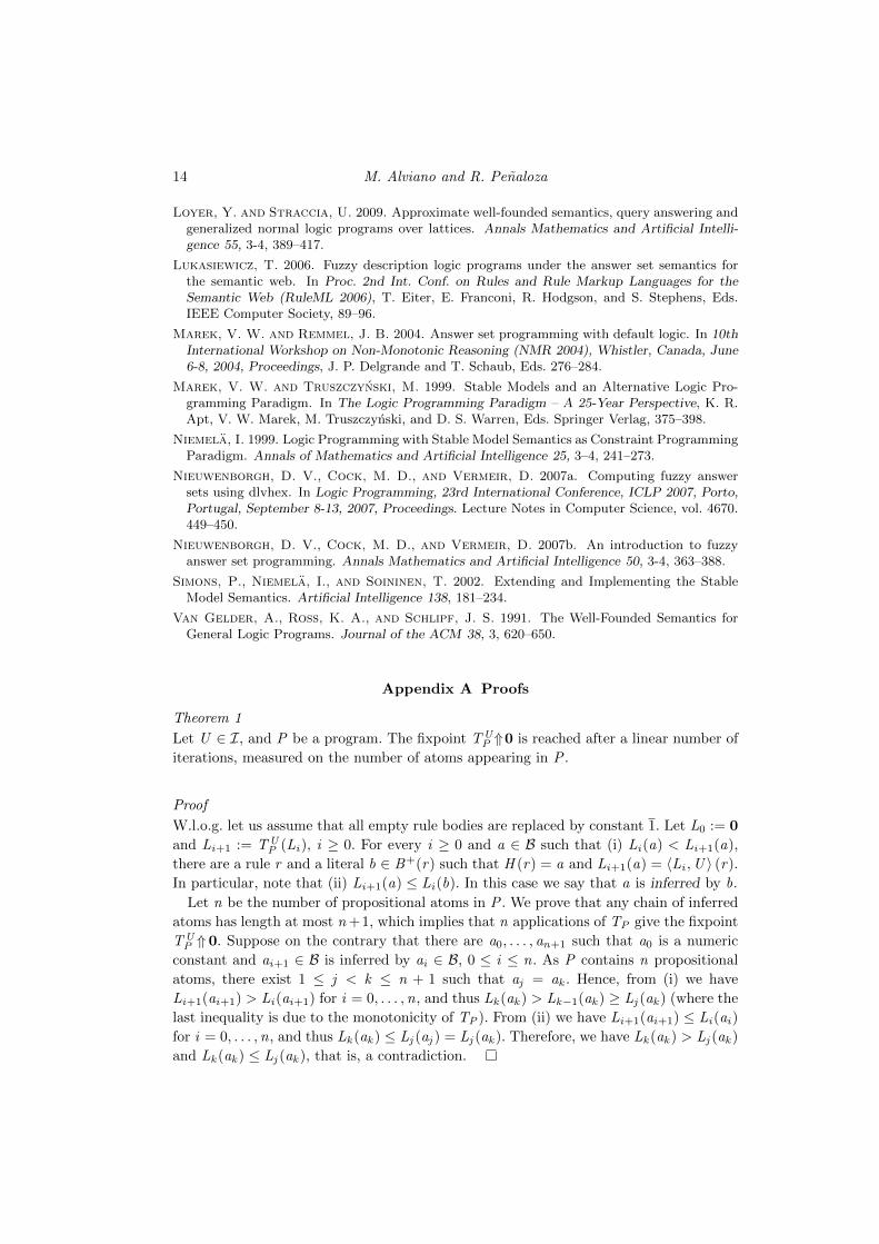
Theorem 1

Let U ∈ I, and P be a program. The fixpoint TUP ⇑0 is reached after a linear number of

iterations, measured on the number of atoms appearing in P .

Proof

W.l.o.g. let us assume that all empty rule bodies are replaced by constant 1. Let L0 := 0

and Li+1 := TUP (Li), i ≥ 0. For every i ≥ 0 and a ∈ B such that (i) Li(a) < Li+1(a),

there are a rule r and a literal b ∈ B+(r) such that H (r) = a and Li+1(a) = 〈Li ,U 〉 (r).

In particular, note that (ii) Li+1(a) ≤ Li(b). In this case we say that a is inferred by b.

Let n be the number of propositional atoms in P . We prove that any chain of inferred

atoms has length at most n +1, which implies that n applications of TP give the fixpoint

TUP ⇑ 0. Suppose on the contrary that there are a0, . . . , an+1 such that a0 is a numeric

constant and ai+1 ∈ B is inferred by ai ∈ B, 0 ≤ i ≤ n. As P contains n propositional

atoms, there exist 1 ≤ j < k ≤ n + 1 such that aj = ak . Hence, from (i) we have

Li+1(ai+1) > Li(ai+1) for i = 0, . . . ,n, and thus Lk (ak ) > Lk−1(ak ) ≥ Lj (ak ) (where the

last inequality is due to the monotonicity of TP ). From (ii) we have Li+1(ai+1) ≤ Li(ai)

for i = 0, . . . ,n, and thus Lk (ak ) ≤ Lj (aj ) = Lj (ak ). Therefore, we have Lk (ak ) > Lj (ak )

and Lk (ak ) ≤ Lj (ak ), that is, a contradiction.

Fuzzy Answer Sets Approximations 15

Theorem 2

For FASP programs without numeric constants and crisp sets, Definition 2 coincides with

the original notion of unfounded set by Van Gelder et al. (1991).

Proof

Let L,U be crisp sets, L ⊆ U ⊆ B, and P be an ASP program. According to Van Gelder

et al. (1991), a crisp set Y ⊆ B is an unfouded set for P w.r.t. (L,U ) if for each r ∈ P

such that H (r) ∈ Y , (1) B+(r) 6⊆ U , or (2) B−(r) ∩ L 6= ∅, or (3) B+ ∩ Y 6= ∅. Let

X ∈ I be such that X (a) = 1 if a ∈ Y , and X (a) = 0 otherwise. We have to show that

Y is an unfounded set for P w.r.t. (L,U ) (according to Van Gelder et al.) if and only if

X is a fuzzy unfounded set for P w.r.t. (L,U ) (according to Definition 2).

(⇒) Consider a rule r ∈ P such that X (H (r)) > 0. We have H (r) ∈ Y . Any of (1), (2)

and (3) implies 〈U ∩ (1 \X ),L〉 (r) = 0.

(⇐) Consider a rule r ∈ P such that H (r) ∈ Y . We have X (H (r)) = 1, and hence

0 = [U ∩ (1 \X )](H (r)) ≥ 〈U ∩ (1 \X ),L〉 (r) = 0. We prove that if (1) and (3) do not

hold, then (2) holds. Falsity of (3) implies 〈U ∩ (1 \X ),L〉 (r) = 〈U ,L〉 (r), and falsity

of (1) implies 〈U ,L〉 (r) = L(not B−(r)). Therefore, there is an element b of B−(r) such

that L(b) = 1, and hence B−(r) ∩ L 6= ∅, i.e., condition (2) is satisfied.

Theorem 3

Let X1,X2 be two fuzzy unfounded sets for P w.r.t. (L,U ). Then also X1 ∪ X2 is an

unfounded set for P w.r.t. (L,U ).

Proof

Let X = X1 ∪ X2 and r ∈ P such that X (H (r)) > 0 holds. We have to show that

[U ∩ (1 \ X )](H (r)) ≥ 〈U ∩ (1 \X ),L〉 (r). Assume w.l.o.g. that X (H (r)) = X1(H (r)).

Since X1 is unfounded, it follows that

[U ∩(1\X )](H (r)) = [U ∩(1\X1)](H (r)) ≥ 〈U ∩ (1 \X1),L〉 (r) ≥ 〈U ∩ (1 \X ),L〉 (r),

which proves the result.

Theorem 4

M is a fuzzy answer set of a program P if and only if GUSM ,MP = 1 \M .

Proof

(⇒) Since 1 \ (1 \ M ) = M and M |= P , 1 \ M is an unfounded set. Moreover, we

can prove that for any unfounded set X for P w.r.t. (M ,M ), M ∩ (1 \ X ) |= PM

holds, from which X ⊆ 1 \ M follows, since M is a minimal model of PM . Consider

a rule r ∈ P . As the interepretation of B−(r) is fixed in the reduct PM , we have to

show that [M ∩ (1 \ X )](H (r)) ≥ 〈M ∩ (1 \X ),M 〉 (r) holds. If X (H (r)) = 0, then

[M ∩(1\X )](H (r)) = M (H (r)) ≥ 〈M ,M 〉 (r) ≥ 〈M ∩ (1 \X ),M 〉. Otherwise, it follows

that [M ∩ (1 \X )](H (r)) ≥ 〈M ∩ (1 \X ),M 〉 by Definition 2. Thus, GUSM ,MP = 1 \M .

(⇐) Let GUSM ,MP = 1\M . We first show that M |= P . Let r ∈ P . If [1\M ](H (r)) = 0,

then M |= r because M (H (r)) = 1. If [1 \ M ](H (r)) > 0, then M |= r follows from

Definition 2 and the fact M ∩ (1 \ (1 \M )) = M . Hence M |= P , which in turn implies

M |= PM . We now prove that for any M ′ ⊆ M such that M ′ |= PM , X = 1 \ M ′ is

16 M. Alviano and R. Penaloza

an unfounded set for P w.r.t. (M ,M ), from which X ⊆ GUSM ,MP = 1 \ M and thus

M ′ = M . Consider a rule r ∈ P such that X (H (r)) > 0. Since M ′ |= PM , it holds

that M ′(H (r)) ≥ 〈M ′,M 〉 (r). From M ′ = 1 \ X and M ′ ⊆ M , it then holds that

[M ∩ (1 \ X )](H (r)) = M ′(H (r)) ≥ 〈M ′,M 〉 (r) = 〈M ∩ (1 \X ),M 〉 (r), which shows

that X is an unfounded set.

Theorem 5

Let L,U ∈ I, L ⊆ U , and P be a program. If 1\RL,UP ⇓1 ⊆ U , then RL,U

P ⇓1 = GUSL,UP .

Proof

(⊆) We show that X = RL,UP ⇓ 1 is an unfounded set. Consider r ∈ P such that

X (H (r)) > 0. We have to show that [U ∩ (1 \ X )](H (r)) ≥ 〈U ∩ (1 \X ),L〉 (r). Since

1 \ X ⊆ U , we can equivalently show [1 \ X ](H (r)) ≥ 〈U ∩ (1 \X ),L〉 (r). As X is

a fixpoint of RL,PP , we have X (H (r)) ≤ 1 − 〈U ∩ (1 \X ),L〉 (r), which implies that

1−X (H (r)) ≥ 〈U ∩ (1 \X ),L〉 (r).

(⊇) Let now Y be an unfounded set. We will show that (i) RL,UP (Y ) = Y and (ii) I ⊆ J

implies RL,UP (I ) ⊆ RL,U

P (J ), from which we derive Y ⊆ RL,UP ⇓1. To show (i), consider

a ∈ B. If Y (a) = 0, then also RL,UP (Y ) = 0 by definition. Let now Y (a) > 0, and

suppose that there is some r ∈ P such that Y (a) > 1 − 〈U ∩ (1 \Y ),L〉 (r). This is

equivalent to 1 − Y (a) < 〈U ∩ (1 \Y ),L〉 (r). Since Y is unfounded, it must hold that

[U ∩ (1 \Y )](a) ≥ 〈U ∩ (1 \Y ),L〉 (r), and thus we have that

[U ∩ (1 \Y )](a) ≥ 〈U ∩ (1 \Y ),L〉 (r) > 1−Y (a),

which is a contradiction with the fact that [U ∩ (1 \ Y )](a) ≤ 1 − Y (a) must hold. To

show (ii), we just note that 1 − 〈U ∩ (1 \ I ),L〉 (r) ≤ 1 − 〈U ∩ (1 \ J ),L〉 (r) holds for

every r ∈ P .

Theorem 6

Let L,U ∈ I and P be a program. The fixpoint RL,UP ⇓1 can be computed in polynomial

time on the size of P .

Proof

It is easy to see that one application of the RP operator requires linear time in the

number of rules P . Moreover, as in Theorem 1, the greatest fixpoint RL,UP ⇓1 is obtained

after at most as many applications of this operator as there are atoms in P . In total, this

means that this fixpoint can be computed in polynomial time on the size of P .

Theorem 7

Let P be a program, L,U two interpretations, (L′,U ′) = WP (L,U ), and M an answer

set of P . If L ⊆ M ⊆ U , then L′ ⊆ M ⊆ U ′.

Proof

By definition, L′(a) = [TUP (L)](a) = max〈L,U 〉 (r) | H (r) = a. By assumption,

L ⊆ M ⊆ U and hence 〈L,U 〉 (r) ≤ 〈M ,M 〉 (r) = M (B(r)) for every rule r . Since M is

a model of its reduct, we have L′(a) ≤ maxM (B(r)) | H (r) = a ≤ M (a).

On the other hand, since M is an answer set of P , by Theorems 4 and 5 it follows that

1 \M = GUSM ,MP = RM ,M

P ⇓1 ⊇ RL,UP ⇓1. This implies that M ⊆ 1 \RL,U

P ⇓1 = U ′

Fuzzy Answer Sets Approximations 17

Theorem 8

Let P be a stratified program. The least fixpoint of WP coincides with the unique answer

set of P and is computable in polynomial time.

Proof

The fact that WP ⇑ (0,1) is the unique answer set of P follows using the same ideas

presented in (Lukasiewicz 2006). Each application of WP requires a computation of TP

and one of RL,UP ⇓ 1, each of which is polynomial on the number of atoms in P . An

increase of L(a) in the i -th iteration of WP is caused by an increase of L(b) or a decrease

of U (b) in the previous iteration, for some b ∈ B. As in the proof of Theorem 1, this

implies that at most linearly many iterations (on the number of atoms appearing in P)

can be applied before a fixpoint is reached.

Theorem 9

Let L,U ∈ I, and P be a program. If M |= P and L ⊆ M ⊆ U , then SUP (L) ⊆ M ⊆ U .

Proof

Since M |= P and L ⊆ M , we have that [SUP (L)](a) ≤ M (a) for every atom a ∈ B, and

hence SUP (L) ⊆ M .

Theorem 10

Let P be a program over the Lukasiewicz t-norm, and L,U ∈ I. For every atom a ∈ Bit holds that [SU

P (L)](a) = minI (a) | I satisfies LP ∪ L(b) ≤ I (b) ≤ U (b) | b ∈ B.

Proof

Let r be a rule of the form (1), and I an interpretation. I |= r if and only if

I (a) ≥ I (B(r)) = maxI (b1) + . . .+ I (bm)− I (bm+1)− . . .− I (bn) + 1−m, 0.

Since I (a) ≥ 0, I |= P if and only if I satisfies the system LP . Additionally, L ⊆ I ⊆ U

if and only if for every b ∈ B it holds that L(b) ≤ I (b) ≤ U (b). Finally, as the feasible

region is closed, the optimal can be reached.

Theorem 11

Let L,U ∈ I, and P be a program over the Lukasiewicz t-norm. SUP (L) is computable

in polynomial time w.r.t. the number of rules.

Proof

The computation of the SP operator requires to solve one linear programming problem

for each atom a appearing in P . Linear programming is well-known to be solvable in

polynomial time on the number of restrictions. As the size of LP corresponds to the

number of rules in P , this yields a polynomial complexity upper bound.

Theorem 12

The fixpoint of WP gives the well-founded semantics by Damasio and Pereira (2001).

18 M. Alviano and R. Penaloza

Proof

The well-founded semantics by Damasio and Pereira (2001) is defined as the fixpoint of

the following operator (adapted to our notation):

Ω(L,U ) := (TUP ⇑0,TL

P⇑0)

Let U ′ := TLP⇑0. The claim immediately follows by Theorem 5 and the following property

(proved below):

U ′ ⊆ U =⇒ 1 \U ′ = GUSL,UP .

We first prove that 1 \ U ′ is unfounded w.r.t. (L,U ). Let r be a rule in P such that

U ′(H (r)) > 0. We have

[U ∩ (1 \ (1 \U ′)](H (r)) = [U ∩U ′](H (r)) = U ′(H (r))

≥ max〈U ,L〉 (r ′) | r ′ ∈ P ,H (r ′) = H (r)≥ 〈U ,L〉 (r)

≥ 〈U ∩U ′,L〉 (r)

= 〈U ∩ (1 \ (1 \U ′)),L〉 (r).

We complete the proof by proving X ⊆ 1 \ U ′, or equivalently U ′ ⊆ 1 \ X , for every

unfounded set X w.r.t. (L,U ). To this aim, let Un be the n-th application of TUP to 0,

n ≥ 0. We prove Un ⊆ 1 \X by induction on n ≥ 0.

For n = 0, the result holds trivially, since U0 = 0. Suppose now that Un ⊆ 1\X holds

for n ≥ 0 in order to show Un+1 ⊆ 1\X . Since TP is monotonic, we know that Un ⊆ U ′.

By combining with the induction hypothesis and the original assumption U ′ ⊆ U , we

have that Un ⊆ U ∩ (1 \X ). Consider now an atom a such that X (a) > 0. We have

Un+1(a) = max〈(Un ,L〉 (r) | r ∈ P ,H (r) = a≤ max〈U ∩ (1 \X ),L〉 (r) | r ∈ P ,H (r) = a≤ [U ∩ (1 \X )](a) (A1)

≤ [1 \X ](a),

where line (A1) follows from the assumption that X is an unfounded set w.r.t. (L,U ).

Hence, Un+1(a) ≤ 1−X (a) holds for every a ∈ B, which complete our proof.