133 * Corresponding author email address: [email protected]Fuzzy motion control for wheeled mobile robots in real-time Mohammad Hossein Falsafi, Khalil Alipour * and Bahram Tarvirdizadeh Advanced Service Robots (ASR) Laboratory, Department of Mechatronics Engineering, Faculty of New Sciences and Technologies, University of Tehran, Tehran, Iran Article info: Abstract Due to the various advantages of Wheeled Mobile Robots, many researchers have focused on solving their challenges. The automatic motion control of such robots is an attractive problem and is one of the issues which should carefully be examined. In the current paper, the trajectory tracking problem of Wheeled Mobile Robots which are actuated by two independent electrical motors is deliberated. To this end, and also, computer simulation of the system, first, the system model is derived at the level of kinematics. The system model is nonholonomic. Then a simple non-mode-based controller based on fuzzy logic is proposed. The control input resulted from fuzzy logic is then corrected to fulfill the actuation saturation limits and non-slipping condition. To prove the efficiency of the suggested controller, its response, in terms of the required computational time burden and tracking error, is compared with a previously suggested method. The obtained simulation results support the superiority of fuzzy-based method over a previous study in terms of the considered measures. Received: 11/01/2017 Accepted: 05/08/2018 Online: 05/08/2018 Keywords: Wheeled mobile robot, Motion control, Fuzzy logic, Predictive control. 1. Introduction In contrast to fixed-base manipulator arms, mobile robots have an unlimited workspace. This advantage stem from the locomotion mechanisms of such robots. The locomotion of such systems can be wheeled, tracked, legged or combination of them [1]. Due to the various advantages of wheeled locomotion, Wheeled Mobile Robots (WMRs) have extensively been studied. To have an autonomous WMR, capable of performing desired tasks, various autonomy challenges including planning and controlling should be solved. As a result, some researchers have tried to design motion controllers to drive the robot to accomplish their favorite missions [2-5]. Motion control of wheeled robots can be divided into three distinct problems. In the first problem, which is called trajectory tracking, it is desired that the robot is controlled such that the desired trajectories of a reference point of the robot be tracked. In the second problem, which is named path following, the control of the robot is aimed at directing the robot in a way that one of its points can follow a desired geometrical path. In the path following problems, the robot velocity along the path is not controlled. In the last problem, which is known as point stabilization,
into three distinct problems. In the first problem,
which is called trajectory tracking, it is desired
that the robot is controlled such that the desired
trajectories of a reference point of the robot be
tracked. In the second problem, which is named
path following, the control of the robot is aimed
at directing the robot in a way that one of its
points can follow a desired geometrical path. In
the path following problems, the robot velocity
along the path is not controlled. In the last
problem, which is known as point stabilization,
JCARME Mohammad Hossein Falsafi, et al. Vol. 8, No. 2
134
the robot is controlled such that it can reach a
desired point with a favorite orientation.
In many studies, it is assumed that the WMR
travels with a low velocity and it does not slip
laterally and/or longitudinally. This assumption
imposes nonholonomic (analytically non-
integrable) constraints on the robot motion [6].
Based on Brocket theorem, there is no static
smooth feedback of state variables for the point
stabilization [7]. Hence, various control methods
have been presented to stabilize WMRs which
can be categorized into continuous and
discontinuous time controllers. Samson
developed smooth continuous-time controllers
well while the discontinuous controllers were
studied in [8, 9].
Motion control of robots can be classified into
two kinematical and dynamical schemes. In the
kinematic controllers, the input controls are
angular velocities of wheels while dynamic
controllers are designed by considering the
actuating torques of wheels as the adjustable
input control.
Considering parametric uncertainties, an
adaptive controller was suggested for a group of
nonholonomic mechanical systems at the level
of dynamics [10]. Ge et al. [11] examined
stabilization of chained systems using a robust
adaptive algorithm while parametric
uncertainties and external disturbance were
considered. The trajectory tracking of a two-
wheeled robot was examined using the
backstepping technique, while non-parametric
uncertainties and disturbances were taken into
account [12]. Dong et al. [13] designed an
adaptive backstepping controller for both
trajectory tracking and point stabilization A
robust controller was suggested to exponentially
stabilizing of WMRs containing parametric
uncertainties [14]. An adaptive controller was
suggested for WMRs where the motor dynamics
was furthermore considered [15]. The adaptive
sliding mode controller was suggested to track
the designated trajectories in [16].
In addition to the works focused on controlling a
WMR containing a single platform, some
researchers were just recently addressed
controlling a WMR including two platforms [17-
19]. In these works, using actuators of tractor
platform, the motion of trailer platform, whose
wheels are passive, was controlled.
In most of the above-mentioned studies, the
control law was devised based on the accurate
model or the model with some uncertainties. The
control laws which depend on the model suffer
from several drawbacks. Therefore, the first
contribution of the current paper is utilizing
Fuzzy Control (FC) method, which is a non-
model based controller, to the tracking-error
control of the differentially-driven WMR. The
second benefit of the present research is the
assessment of the proposed FC-based algorithm
versus the work done by Gregor, and Igor [2].
The benefits of the developed FC over the Model
Predictive Control (MPC) are examined in the
current study. Besides, the performances of the
FC versus MPC in trajectory tracking of the
WMR are analyzed from two points of view. The
first one is the path tracking error and the second
one is the processing time duration.
After this introduction, the remainder of the
present study is organized as described. In the
next section, the model of WMR at the level of
kinematics is rendered which is followed, in
section 3, by some prerequisite material required
for its motion control. Then, the suggested fuzzy
based method and model predictive one are
introduced in detail in sections 4 and 5,
correspondingly. In succeeding section, the
obtained results of the forgoing control
techniques are compared. The conclusions of the
paper will be addressed in the last section.
2. Modeling of WMR
In the present section, the kinematics model of
the robot system is detailed. Then, the control
problem regarding trajectory tracking of the
robot is defined.
2.1. WMR kinematic model
The robotic system which is to be modeled
consists of two active wheels and a single
passive wheel. The passive wheel is added to the
robot platform to improve its stability. To derive
the system kinematics, two frames are attached
to the mobile platform as depicted in Fig. 1. The
Z presents the world-coordinate frame while
JCARME Fuzzy motion control for . . . Vol. 8, No. 2
135
denotes its body-coordinate frame which
is completely attached to the robot and travels
with it. The two active wheels are actuated by
two independent electrical DC motors. The
considered motors can provide the commanded
feasible angular velocity. It should be noted that
the passive wheel is a kind of caster or spherical
type. Notice that while the number of passive
wheels may affect the postural stability of the
system, it does not change the kinematics of it.
The robot center of mass is located at point G
while point O denotes the mid-point of the line
connecting the center of two active wheels. The
distance between point O and G is considered as
b (Fig. 1). In the current study, for the sake of
simplicity, b is considered as zero. The robot
pose is represented by coordinates of one of its
points and the heading angle . It is also worth
mentioning that the origin of coordinates
frame relative to Z frame is denoted by
0 0( , )Z . Likewise, the coordinates of point G in
inertial frame are represented as G G( , )Z . The
distance between the active wheels center is
considered as D. The rotational velocities of
right and left wheels around their axels are
represented by R and L , respectively.
Moreover, the wheels radius is denoted as .
G
O
Support wheel
ϑ
Z
ϒ
ZGZ0
ϒG
ϒ0
ρ
υ
Db
Fig. 1. The three-wheeled robot configuration along
with its geometrical parameters.
The robot configuration parameters are denoted
by vector G GT
Z μ . In the current
research, it is supposed the robot moves on a flat
terrain. Also, the robot, wheels, as well as terrain
are assumed to be rigid. Wheels are subjected to
pure rolling. This means that the robot wheels do
not slip either laterally or longitudinally. Based
on Fig. 2, if the angular velocity of the robot is
represented by Ω , then the linear velocity of the
robot wheels center can be written as follows:
R o R OS = S +Ω×d (1)
L o L ΟS = S +Ω×d (2)
where SR and SL indicate the linear velocity of
the right and left wheels center, respectively.
Besides, SO represents the point O linear
velocity. Also, R Od and L Οd indicate the
position of the right and left wheels center
relative to point O, respectively.
If the unit vectors of the robot body coordinate
frame along , and directions are
considered as 𝐮𝟏, 𝐮𝟐 and 𝐮𝟑 , respectively, then
the following relations can be written:
3 2. ( . ) ( )2
RD
S S 1 1u u u u (3)
3 2. ( . ) ( )2
LD
S S 1 1u u u u (4)
In the above equations, SR and SL denote the
speed of the right and left wheels center,
correspondingly. Moreover, ‘×’ indicates the
operator of the vector outer product.
O
SO
SR
SL
Ω
ϑ
Z
ϒ
Fig. 2. The kinematic diagram of the DDWMR.
JCARME Mohammad Hossein Falsafi, et al. Vol. 8, No. 2
136
Using the last two relations, one can obtain the
following equation:
.1 / 2 1 / 22
1/ 1 /.
2
RR
LL
DS S
S
D DDS S
(5)
According to the above equation, one can claim
that a one-to-one relationship exists between the
actual input controls of the robot, namely R
and L , and its linear/angular velocity. Hence,
instead of robot rotational velocities, one can
easily utilize S and as the control input, as
will be observed in Section 4.
As mentioned previously, the robot wheels do
not slip. Hence, the point O linear velocity will
simply be in the axis direction. Therefore, it
can be concluded that GZ S c and
G S s in which s() and c() stand for sin()
and cos() functions, respectively. If the relation
is added to the equations denoting the two
components of linear velocity of point O, then
the following vector/matrix equation results:
0
0
0 1
cS
s
μ (6)
2.2. Maximum translational and rotational
speeds
To address the issue of actuators limitations in
the controller design process, the process
proposed by Gregor, and Igor [2] is followed.
Herein, this technique is elaborated. In this
process, it is required that the maximum
translational and rotational speeds of the robot
that can be produced by actuators are computed
according to the extreme angular velocities of
the motors. If the extreme rotational velocity of
the wheels is denoted by max , then one can claim
that the maximal linear velocity of the WMR is
generated when two motorized wheels are
rotating with max . Consequently, the following
equation can be written:
max max
max
2
R L
R L
SS
(7)
Likewise, once the two motorized wheels are in
motion in contrast directions with maximum
angular velocity, the maximal angular velocity is
resulted. Therefore, the following result is
obtained.
max max
max
2R L
R L
DD
(8)
By defining the factor α based on the ratio of
translational/rotational speeds, and the
maximum max max/ S , as follows, the initial
control command can be corrected as:
maxmax
max
maxmax
max
max max
)
sign( ). ,
)
, sign( ).
) ,
1 ,
c
c c
c
c c
c c
c c
SS S
S
S S S
SS
S S
S S
(9)
max max
max , , 1S
S
It should be emphasized that the above relations
can be resulted based on the point that if one of
the linear or rotational speed is modified, the
other one should also be corrected so as the
curvature radius of the path traveled by the
WMR can be kept [2]. Note that in the above
relations, sign(.) denotes the function of signum.
In addition to the above modifications of the
control inputs, to avoid the robot slipping, the
robot acceleration should not be exceeded some
specified threshold (represented by be βmax), [2].
To address the wheeled robot acceleration
constraint, according to the definition of the
acceleration, one should pay attention to the
JCARME Fuzzy motion control for . . . Vol. 8, No. 2
137
robot velocity history. Hence, the following
equations can be written:
max
max
max
max
max
max
( )
( ) ( 1)
sign( ). .
( )
( )
( 1) sign( ). .
R Rc R
R
Rc R
R s
L Lc L
L Lc
L L s
S S i
S i S i
S
S S i
S i
S i S
(10)
Note that in the above relations, R and L
represent the acceleration of the right and left
wheels centers, accordingly. In addition, SRc and
SLc indicate the linear control command
associated with the WMR right and left wheels,
respectively. Moreover, Ss represents the
sampling time. It is worth to mention that βmax,
which can be computed experimentally, is
strongly intertwined with the features of the
robot actuators.
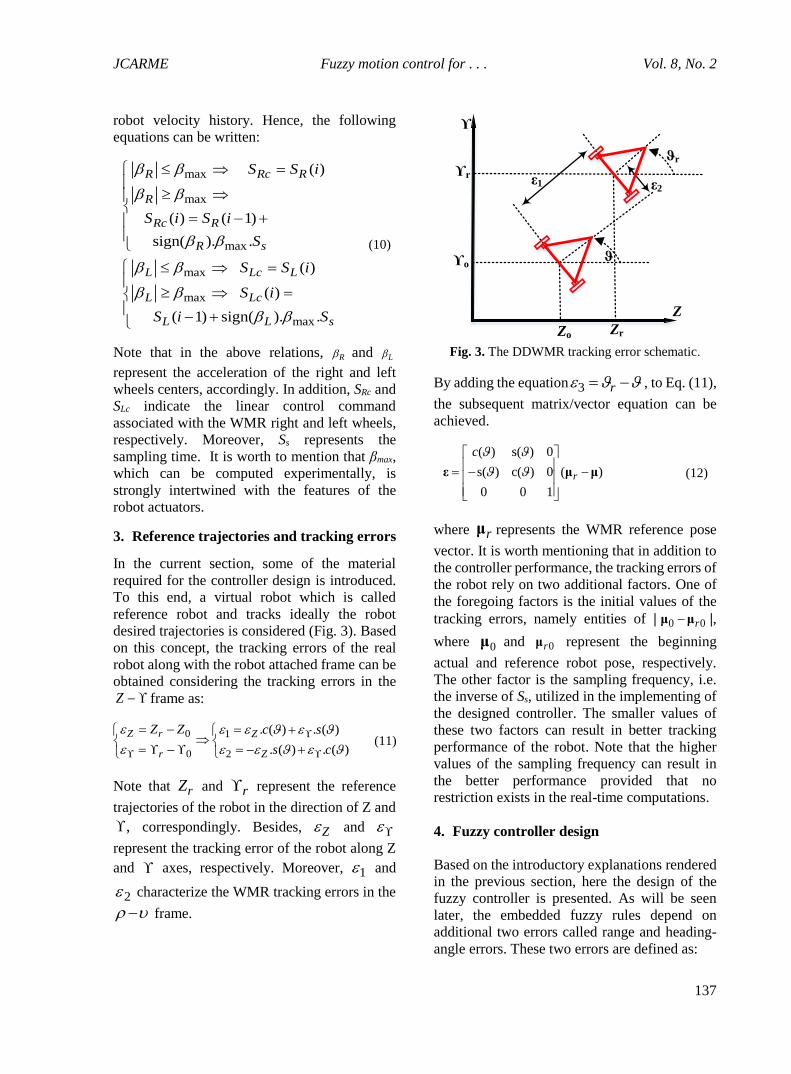
3. Reference trajectories and tracking errors
In the current section, some of the material
required for the controller design is introduced.
To this end, a virtual robot which is called
reference robot and tracks ideally the robot
desired trajectories is considered (Fig. 3). Based
on this concept, the tracking errors of the real
robot along with the robot attached frame can be
obtained considering the tracking errors in the
Z frame as:
0 1
0 2
. ( ) . ( )
. ( ) . ( )
Z r Z
r Z
Z Z c s
s c
(11)
Note that rZ and r represent the reference
trajectories of the robot in the direction of Z and
, correspondingly. Besides, Z and
represent the tracking error of the robot along Z
and axes, respectively. Moreover, 1 and
2 characterize the WMR tracking errors in the
frame.
Zo
ϒo
Zr
ϒr
ϑr
ε1 ε2
Z
ϒ
ϑ
Fig. 3. The DDWMR tracking error schematic.
By adding the equation 3 r , to Eq. (11),
the subsequent matrix/vector equation can be
achieved.
( ) s( ) 0
s( ) c( ) 0 ( )
0 0 1
r
c
ε μ μ (12)
where rμ represents the WMR reference pose
vector. It is worth mentioning that in addition to
the controller performance, the tracking errors of
the robot rely on two additional factors. One of
the foregoing factors is the initial values of the
tracking errors, namely entities of | 0 0rμ μ |,
where 0μ and 0rμ represent the beginning
actual and reference robot pose, respectively.
The other factor is the sampling frequency, i.e.
the inverse of Ss, utilized in the implementing of
the designed controller. The smaller values of
these two factors can result in better tracking
performance of the robot. Note that the higher
values of the sampling frequency can result in
the better performance provided that no
restriction exists in the real-time computations.
4. Fuzzy controller design
Based on the introductory explanations rendered
in the previous section, here the design of the
fuzzy controller is presented. As will be seen
later, the embedded fuzzy rules depend on
additional two errors called range and heading-
angle errors. These two errors are defined as:
JCARME Mohammad Hossein Falsafi, et al. Vol. 8, No. 2
138
𝜀𝑏 = √𝜀12 + 𝜀2
2 (13)
𝜀𝜗 = tan−1(𝜀2 𝜀1⁄ ) (14)
where εb specifies the range error, and
indicates the heading error. To generate the
control signals based on the developed fuzzy
method, first the errors Z and should be
converted to εb and . In this regard, a block is
considered in the block-diagram of the suggested
control method, as can be observed in Fig. 4. The
developed fuzzy controller generates the WMR
input signals, S and Ω, based on εb and . It
should be pointed out that the robot can
compensate the distance error by the linear
velocity and the angular error by the angular
velocity. Hence, the controller design based on
εb and is beneficial. Indeed, adopting these
errors removes the cross-coupling problem once
the rule-base is generated. As a result,
composing the fuzzy rules is simplified.
A fuzzy-based controller consists of various
features. The first feature is called fuzzification.
This feature is formed based on membership
functions (MFs) and by which a crisp value is
transformed to a fuzzy value. The second
element of a fuzzy controller is named rule-base
and consists of a set of “if-then” rules. The third
part of a fuzzy controller is known as
defuzzification which converts a fuzzy value to
a crisp value. Fig. 5 to 8 describe the MFs for εb,
, S and , correspondingly. Note that the
whole aforementioned MFs are obtained by
adopting trial and error approach.
The value of WMR translational velocity is
categorized into several Linguistic Variables
(LVs) as depicted in Table 1. This table also
states the linguistic variables of range error εb.
Besides, in Table 2, the linguistic variables
associated with WMR rotational velocity and the
heading error are given.
Trajectory
Planning
Error
Mapping
Fuzzy Motion
ControllerWheeled Robot
Zr
ϒr
Zϒ
ϑ
εZ
εϒ
εb
εϑ
S
Ω
Fig. 4. The developed fuzzy control algorithm.
Fig. 5. The MFs of the range error “εb”.
Fig. 6. The MFs of the heading error “ ”.
Wheeled robot Fuzzy motion
controller
Error
mapping
Trajectory
planning
JCARME Fuzzy motion control for . . . Vol. 8, No. 2
139
Fig. 7. The MFs of the linear velocity “S”.
Table 1. The LVs for WMR translational speed and
range error εb.
The LVs associated with
S
The LVs associated with
WMR range error
𝑉𝑉𝑆 →Very very slow
VS→Very slow
S→Slow
M→Medium
F→Fast
VF→Very fast
VVF→Very very fast
Z→Zero
VN→Very near
N→Near
M→Medium
F→Far
VF→Very far
VBF→Very big far
Table 2. The LVs for WMR rotational speed and
heading error .
The LVs associated with
The LVs associated with
WMR heading error
VSN→ Very small negative
SN→ Small negative
N→ Negative
Z→ Zero
P→ Positive
BP→ Big positive
VBP→ Very big positive
VSN→Very small negative
SN→ Small negative
N→ Negative
Z→ Zero
P→ Positive
BP→ Big positive
VBP→ Very big positive
In Table 3, the employed rule-bases are
reflected. It is worth mentioning that in the
present study, the fuzzy inference system is of
type Mamdani [20]. In addition, for the output-
defuzzification purposes, the method of
“centroid” is exploited.
Fig. 8. The MFs of the rotational velocity “ ”.
Desired
trajectory
generator
Open-loop
control
Coordinate
change
Model
predictive
control
Wheeled
robot+
Unit of control
-
Fig. 9. The control topology utilized by Klančar, and Škrjanc [2] to motion control of the WMRs.
JCARME Mohammad Hossein Falsafi, et al. Vol. 8, No. 2
140
Table 3. The utilized rule-base for constructing WMR control inputs.
The FC rule-bases for S The FC rule-bases for If εb is Z then 𝑆 is VVS If is VSN then is VSN
If εb is VN then 𝑆 is VS If is SN then is SN
If εb is N then 𝑆 is S If is N then is N
If εb is M then 𝑆 is M If is Z then is Z
If εb is F then 𝑆 is F If is P then is P
If εb is VF then 𝑆 is VF If is BP then is BP
If εb is VBF then 𝑆 is VVF If is VBP then is VBP
5. An overview of MPC design To study the response of the suggested controller, in terms of tracking performance and the required computational time, an attractive control strategy based on MPC is utilized. In the present study, the MPC controller, presented by Gregor, and Igor [2], to adjust the motion of WMRs is exploited. Therefore, in the present section, this control method is summarized. Fig. 9 illustrates the presented control topology. The aforementioned controller is realized based on the combination of two open- and closed-loop controls. In fact, like many tracking controllers, some of the nonlinearities are canceled by adopting feedforward strategy, and the system is prepared for fine tuning by MPC-based closed-loop. Consequently, the vector of WMR control input ν can be written as:
𝛎 = 𝛎𝐹𝐹 + 𝛎𝐹𝐵 (15)
where 𝛎𝐹𝐹 and 𝛎𝐹𝐵 represent the open-loop (feedforward) and closed-loop slices of the control signal, correspondingly. To calculate the feedforward control signal, first, the translational and rotational angular velocities, as well as the reference heading angle of WMR, should be calculated. The aforementioned quantities can be attained as:
2 2
r r rS Z (16)
tan 2( , )r
A ir rZ (17)
2 2
. .r r r rr
r r
Z Z
Z
(18)
In the above equation, rS , r and r represent
the favorite translational speed, desired orientation and reference rotational speed, correspondingly. According to these factors, the feedforward signal, 𝛎𝐹𝐹 , can be written as follows:
𝛎𝐹𝐹 = [𝑆𝑟 Ω𝑟. 𝑐(𝜀3)]𝑇 (19)
After obtaining the feedforward signal, the feedback signal is derived. To this end, first, the error dynamics is obtained. In this direction, Eq. (12) is differentiated with respect to the time which leads to the following relation:
s c 0
c s 0 ( )
0 0 0
c s 0
s c 0 ( )
0 0 1
r
r
ε μ - μ
μ - μ
(20)
Now, according to Eq. (6), terms μ and rμ are
substituted which leads to the next equation:
c( ) 0 1 0
s( ) 0 0 0
0 1 0 1
s c 0
c s 0 ( )
0 0 0
r
r
r
r
r
S
ε μ - μ
ν
(21)
By substituting Eq. (15) for ν and considering Eq. (19), the following equation is obtained:
3
0 0
0 0
0 0 0
0 1 0
s( ) 0 0
0 0 1
r FBS
ε ε
ν
(22)
Note that the above equation is obtained
considering 3 r and linearizing the
error dynamics around the reference trajectory
JCARME Fuzzy motion control for . . . Vol. 8, No. 2
141
(ε1=ε2=ε3=0). After that, the following consequences are achieved:
clscls FB
ε ε νA B (23)
In the above equation, Acls and Bcls are:
0 0
0 ,
0 0 0
cls r
r
r S
A
1 0
0 0
0 1
cls
B (24)
The above differential vector equation can be transformed into different equation as:
( 1) ( ) ( )i i i FBε A ε B ν
( ),cls s cls sS S A I A B B (25)
According to the above linear equation, designing an MPC is possible. To this end, a quadratic performance index representing the tracking error and control effort is established as:
1
( , ). . ( , )( , )
( , ). . ( , )
Th
i
i j i ji
i j i j
B T
B B
e W eν
ν T ν (26)
Notice that in Eq. (26), h indicates the time
horizon. Also, ( , ) ( ) ( | )i j k j i j i re ε ε ,
in which ( )i jrε characterizes the reference
WMR error. Besides, ( | )i j iε denotes the
estimated error of the actual WMR at sample time of (i+j) according to the data of the first i sampling periods. Also, W is a square semi positive matrix with dimension n. Likewise, T characterizes a square positive definite scaling matrix with dimension m. It is pointed out that in the current study, the value of n is set as 3 while m is equal to 2. The closed-loop part of the
control input signal, Bν , is attained by
extremizing the aforementioned performance
index , as:
( ) ( )FB mpci iν F ε (27)
in which mpcF is calculated according to the next
equations:
mpc -1
T T
rF H QH + T H W v - v (28)
where
( )
( | )
( 1| ). ( )
( ,1). ( | )
0 0
( 1| )
( ,2). ( 1| ) ( 1| )
i
i i
i i B i i
i B i i
i i
i i i i h i
H
B
A
Δ
B
Δ B B
1
( , ) ( | )
h
k j
i j i k i
AΔ
(h.n) (h.n)
0 0
0 0
0 0
W
W
W
W
(h.m) (h.m)
0 0
0 0
0 0
T
T
T
T
( ) ( | ) ( 1| ). ( | )
.... ( ,0)T
k i i i i i i
i
v A A A
Δ
2....
Th
r r r r
v A A A
( 1) ( ). ( )jr ri i i ε ε , j=1,…, h
(29)
6. The response of the suggested fuzzy based controller against MPC
To assess the response of the proposed controller against MPC, various maneuvers can be considered. In the present section, the response of one of these maneuvers will be detailed. The supposed favorite trajectories in the inertial coordinate frame for the robot to track is:
1.1 0.7 s 0.209
0.9 0.7 0.4189
r
r
Z t
c t
(30)
in which, 𝑡 = [0 ∼ 30] sec. Also, the sampling time Ss is set as 0.1 sec. The performance of the fuzzy control based method and that of MPC is examined in terms of two measures. The first important vector addresses the trajectory
JCARME Mohammad Hossein Falsafi, et al. Vol. 8, No. 2
142
tracking precision while the next one requires processing time duration. For the supposed maneuver, it is assumed that the robot initiates its motion with an initial distance to the desired trajectories. Besides, due to the real-world conditions and actuator limitations, it is assumed that the extreme translational and rotational accessible speeds are SMAX=0.5m/s and ΩMAX=13rad/s. In addition, to avoid the robot wheels from slipping, it is also assumed that the wheels translational acceleration is at most βMAX = 3m/s2.
6.1. Trajectory tracking error assessment
In this subsection, the performance of the two controllers are explored in terms of tracking precision. In this regard, the simulation results obtained are depicted in Figs. 10 and 11. As observed, while both controllers can lead to the successful tracking of WMR, the fuzzy-based controller can push the robot to the prescribed trajectories sooner as compared to the MPC. The total tracking error is computed for the two mentioned controllers using the following equation:
( ) ( ) ( ) ( )ultimate
initial
t t
r rt t
Error Z t Z t t t
(31)
Fig. 10. The path followed by the WMR employing the fuzzy- based method.
Fig. 11. The path followed by the WMR employing the model predictive method.
In Table 4, the response of the two controllers is presented. As seen in this table, the magnitude of tracking error resulted using fuzzy-based technique is less than that originated from MPC.
Table 4. The error resulted from two control methods for the prescribed trajectories.
Method of control Fuzzy Model predictive Error quantity 27.02 37.50
6.2. Required processing time duration
In Fig. 12 and Fig. 13 the required processing time durations, by the central processor, for the both of the fuzzy and the model predictive controllers are demonstrated which are 0.015 (s) and 0.3 (s) in FC and MPC, respectively. This means that the FC can produce the output signals for about 20 times faster than the MPC.
Fig. 12. Processing time for fuzzy model.
Fig. 13. Processing time for MPC.
In addition, the minimum value of the processing time duration limits the minimum value of the sampling time/discretization period. Consequently, the controller processing speed affects the system control performance, implicitly. Considering this point, it can be concluded that the FC performance can be increased as compared with the MPC. The control inputs of the FC and MPC are demonstrated in Fig. 14 and Fig. 15, respectively. As seen, while the angular velocity signal of MPC is better than that of FC, both controllers are successfully fulfilled the limitation
JCARME Fuzzy motion control for . . . Vol. 8, No. 2
143
considered for this control input. Additionally, the linear velocity input of FC seems to be better than that of MPC. However, again both controllers are satisfied their actuator saturation constraints, based on Eqs. (9 and 10).
Fig. 14. Linear and angular velocities in FC.
Fig. 15. Linear and angular velocities in MPC.
7. Conclusions
In the current research, a fuzzy-based method is
suggested for the trajectory tracking control of
WMRs. The considered 3-wheeled robot
contains two motorized wheels along with a
passive wheel. To simulate the system response
and design a kinematical controller, the model of
the robot at the level of kinematics is
derived. Next, a simple but efficient fuzzy
controller is designed, and its response is
examined against a model predictive controller
in terms of two points of view. The first criterion
is the tracking accuracy and the second one is the
required processing time durations. The
achieved simulation results reveal the superior
behavior of the fuzzy-based method against
MPC in terms of both aforementioned
performance indices.
References
[1] L. Bruzzone, and Quaglia Giuseppe,
"Locomotion systems for ground mobile
robots in unstructured environments."
Mechanical Sciences Vol. 3, No. 2, pp.
49-62, (2012).
[2] Gregor Klančar, and Igor Škrjanc.
"Tracking-error model-based predictive
control for mobile robots in real time."
Robotics and Autonomous Systems, Vol.
55, No. 6, pp.460-469, (2007).
[3] Tian Yu, and Nilanjan Sarkar, "Control of
a mobile robot subject to wheel slip."
Journal of Intelligent & Robotic Systems,
Vol. 74, No. 3-4, pp. 915-929, (2014).
[4] Hadi Amoozgar, Mohammad Khalil
Alipour, and Seyed Hossein Sadati, "A
fuzzy logic-based formation controller for
wheeled mobile robots." Industrial Robot:
An International Journal, Vol. 38, No. 3
pp. 269-281, (2011).
[5] Khalil Alipour, and S. Ali A. Moosavian,
"Dynamically stable motion planning of
wheeled robots for heavy object
manipulation." Advanced Robotics, Vol.
29, No. 8, pp. 545-560, (2015).
[6] Kevin M. Lynch, and C. Park Frank,
Modern Robotics: Mechanics, Planning,
and Control, Cambridge University Press,
(2017).
[7] Anthony M. Bloch, Mahmut Reyhanoglu,
and N. Harris McClamroch, "Control and
stabilization of nonholonomic dynamic
systems." IEEE Transactions on
Automatic control, Vol. 37, No. 11, pp.
1746-1757, (1992).
[8] Astolfi, Alessandro, "Discontinuous
control of nonholonomic systems."
Systems & control letters, Vol. 27, No. 1
pp. 37-45, (1996).
[9] Farzad Pourboghrat, "Exponential
stabilization of nonholonomic mobile
robots." Computers & Electrical
JCARME Mohammad Hossein Falsafi, et al. Vol. 8, No. 2
144
Engineering, Vol. 28, No. 5, pp. 349-359,
(2002).
[10] Dong Wenjie, W. Liang Xu, and Wei
Huo, "Trajectory tracking control of
dynamic non-holonomic systems with
unknown dynamics." International
Journal of Robust and Nonlinear Control,
Vol. 9, No. 13, pp. 905-922, (1999).
[11] Ge Shuzhi Sam, J. Wang, Tong Heng Lee,
and G. Y. Zhou, "Adaptive robust
stabilization of dynamic nonholonomic
chained systems." Journal of Field
Robotics, Vol. 18, No. 3, pp. 119-133,
(2001).
[12] Kim, Min-Soeng, Jin-Ho Shin, Sun-Gi
Hong, and Ju-Jang Lee, "Designing a
robust adaptive dynamic controller for
nonholonomic mobile robots under
modeling uncertainty and disturbances."
Mechatronics, Vol. 13, No. 5, pp. 507-
519, (2003).
[13] Dong Wenjie, and K-D. Kuhnert, "Robust
adaptive control of nonholonomic mobile
robot with parameter and nonparameter
uncertainties." IEEE Transactions on
Robotics, Vol. 21, No. 2, pp. 261-266,
(2005).
[14] B. L. Ma, and S. K. Tso,
"Robust discontinuous exponential
regulation of dynamic nonholonomic
wheeled mobile robots with parameter
uncertainties." International Journal of
Robust and Nonlinear Control, Vol. 18,
No. 9, pp. 960-974, (2008).
[15] Markus Mauder, "Robust tracking control
of nonholonomic dynamic systems with
application to the bi-steerable mobile
robot," Automatica, Vol. 44, No. 10, pp.
2588-2592, (2008).
[16] Chih-Yang Chen, S. Li, Tzuu-Hseng,
Ying-Chieh Yeh, and Cha-Cheng Chang,
"Design and implementation of an
adaptive sliding-mode dynamic controller
for wheeled mobile robots."
Mechatronics, Vol. 19, No. 2 pp.156-166,
(2009).
[17] Asghar Khanpoor, Ali Keymasi Khalaji,
and S. Ali A. Moosavian "Modeling and
control of an underactuated tractor–trailer
wheeled mobile robot." Robotica, pp. 35-
12, pp. 2297-2318, (2017).
[18] Ali Keymasi Khalaji, and S. Ali A.
Moosavian." Switching control of a
tractor-trailer wheeled robot. "
International Journal of Robotics and
Automation, Vol. 30, No. 2, pp.1-9
(2015).
[19] Ali Keymasi Khalaji, and S. Ali A.
Moosavian, "Modified transpose Jacobian
control of a tractor-trailer wheeled robot."
Journal of Mechanical Science and
Technology, Vol. 29, No. 9, pp. 3961-
3969, (2015).
[20] Ebrahim H. Mamdani, and Sedrak
Assilian, "An experiment in linguistic
synthesis with a fuzzy logic controller."
International journal of man-machine
studies, Vol. 7, No. 1, pp. 1-13, (1975).
How to cite this paper:
Mohammad Hossein Falsafi, Khalil Alipour and Bahram Tarvirdizadeh,
“Fuzzy motion control for wheeled mobile robots in real-time” Journal of
Computational and Applied Research in Mechanical Engineering, Vol. 8,