Fuzzy Systems and Arti ﬁcial Neural Network - chontech.ac.th fileFuzzy Systems and Arti ﬁcial...

Fuzzy Systems and Artificial Neural Network(224441 )

Siripun Thongchai, Ph.D.

Assistant Professor of Electrical Engineering

[email protected]

Teacher Training in Electrical Engineering

Faculty of Technical Education

King Mongkut’s University of Technology North Bangkok

July 21, 2010

1

Teacher Training in Electrical Engineering

Faculty of Technical Education

King Mongkut’s University of Technology North Bangkok

224441 Fuzzy Systems and Artificial Neural Network

Syllabus (1/2010, GMTE)

Instructor: Siripun Thongchai, Ph.D.

Asst. Prof. of Electrical Engineering

Office: Teacher Training in Electrical Engineering Dept., Room: 44-606

Phone:(66) 0-2913-2500 ext. 3339, 3302, 08-9521-3300, FAX:(66) 0-2587-8255,

Email: [email protected],

Web Site: http://www.te.kmutnb.ac.th/~ics

Office Hours: Friday, 18:00 - 20:00 or by appointment.

Time Schedule:

GMTE 2 (S1), August 2010, Saturday - Sunday: 9:00-16:00 (Room:xx)

Summary: Basic concepts of fuzzy logic, fuzzy sets, fuzzy relations, fuzzy if-then rules, fuzzy implications and

approximate reasoning, fuzzy logic and probability theory. Fuzzy logic in control engineering, information tech-

nology, patterns recongnition, and industrial applications. Fundamental of artificial neural networks, neuron

network architectures, perceptron learning rule, signal and weight vector spaces, single layer perceptrons, mul-

tilayer perceptrons, variations on backpropagation, associative learning, competitive networks, self-organizing

maps, recurrent networks, radial-basis function networks, theory of support vector machines, principal compo-

nents analysis, and applications of artificial neural networks.

Textbook: [12], [16], and [7].

References:

The references are [1], [2], [3], [4], [5], [6], [7], [8], [9], [10], [11], [12], [13], [14], [15], [16], [17], [24], [18], [26], [19],

[20], [21],[23],[25], [22], [27], and [28].

Computer Usage: The student is encouraged to use the software package MATLAB, which includes Simulink,

Control System, Fuzzy Control, and Neural Network Toolboxes.

Homework: You may discuss the homework problems with others, but the work you turn in must be your own.

Grading: There are assignments, a midterm exam and a final. They will count toward the grade as follows.

Assignments 20%

Midterm Exam 25%

Report 1 15%

Report 2 15%

Final Exam 25%

Total 100%

2

Course Outline

No. Description Note Textbooks

1 Introduction to Fuzzy Systems see [12] ch.1,2

2 Sets and Fuzzy Sets, Membership Functions see [16] ch.2,3,4, and [8]

3 Logic and Fuzzy Systems, Development of MF see [16] ch.5,6, and [8]

4 Automated Methods for Fuzzy Systems hw 1 see [16] ch.7, and [8]

5 Fuzzy Systems Simulation, Rule-Based Reduction see [16] ch.8, 9 and [8]

6 Decision Making with Fuzzy Information see [16] ch.10, and [8]

7 Fuzzy Classification and Pattern Recognition Report 1 see [16] ch.11, and [8]

8 Fuzzy Control Systems see [12] ch.3,4, [16] ch.13, and [8]

Exam # 1

9 Introduction to Neural Network see [7] ch. 1, and [8]

10 Learning Processes hw 2 see [7] ch. 2, and [8]

11 Single and Multi-layer Perceptrons see [7] ch. 3, 4, and [8]

12 Radial-Basis Function Networks see [7] ch. 5, and [8]

13 Support Vector Machines Report 2 see [7] ch. 6, and [8]

14 Self-Organizing Maps see [7] ch. 9, and [8]

15 Neural Control see [12] ch.5,6

16 Applications of Neural Algorithms and Systems see [12] ch.7,8, [28] ch. 8, and [8]

Exam # 2

References

[1] M. A. Arbib, P Érdi, and J. Szentágothai. Neural Organization: Structure, Function, and Dynamics. MIT Press

(Bradford), Cambridge, MA, 1998.

[2] G. Chen. Fuzzy Logic in Data Modeling: Semantics, Constraints, and Database Design. Kluwer Academic

Publishers, Norwell, Massachusetts, 1998.

[3] Guanrong Chen and Trung Tat Pham. Introduction to Fuzzy Sets, Fuzzy Logic, and Fuzzy Control Systems.

CRC Press, 2001.

[4] D. Driankov, H. Hellendoorn, and M. Reinfrank. An Introduction to Fuzzy Control. Springer-Verlag Berlin,

USA, 2 edition, 1996.

[5] James A. Freeman and David M. Skapura. Neural Networks: Algorithms, Applications, and Programming

Techniques. Addison Wesley, 1991.

[6] F. M. Ham. Principles of Neurocomputing for Science and Engineering. McGraw-Hill Companies, Inc., 2001.

[7] S. Haykin. Neural Networks : A Comprehensive Foundation. Prentice-Hall, Upper Saddle River, New Jersey, 2

edition, 1999.

[8] J.-S. R. Jang, C.-T. Sun, and E. Mizutani. Neuro-Fuzzy and Soft Computing: A Computational Approach to

Learning and Machine Intelligence. Prentice-Hall, Englewood Cliffs, NJ, 1997.

[9] B. Kosko. Neural Networks and Fuzzy Systems. Prentice-Hall, Englewood Cliffs, New Jersey, 1992.

[10] S. Kumar. Neural Networks: A Classroom Approach. McGraw-Hill Companies, Inc., 2004.

[11] F. L. Lewis, S. Jagannathan, and A. Yesildirek. Neural Network Control of Robot Manipulators and Nonlinear

Systems. Taylor & Francis, Philadelphia, Pennsylvania, 1999.

3

[12] Hung T. Nguyen, Nadipuram R. Prasad, Carol L. Walker, and Elbert A. Walker. A First Course in Fuzzy and

Neural Control. CRC Press, USA, 2003.

[13] Chee-Mun Ong. Dynamic Simulation of Electric Machinery Using Matlab/Simulink. Prentice-Hall, Upper Saddle

River, 1998.

[14] K. M. Passino and S. Yurkovich. Fuzzy Control. Addison Wesley Longman, Menlo Park, California, 1998.

[15] T. Ross. Fuzzy Logic with Engineering Applications. McGraw-Hill Companies, Inc., 1995.

[16] T. Ross. Fuzzy Logic with Engineering Applications. John Wiley and Sons, England, 2 edition, 2004.

[17] T. Takagi and M. Sugeno. Fuzzy identification of systems and its applications to modeling and control. IEEE

Transactions on Systems, Man, and Cybernetics, 15(1):116—132, 1985.

[18] S. Thongchai. Behavior-based learning fuzzy rules for mobile robots. In American Control Conference, Anchor-

age, Alaska, 8-10 May 2002.

[19] S. Thongchai. Fuzzy sliding mode control and its applications. In Proceeding of the 26th Conference of Electrical

Engineering, (EECON’26), Chauum, Petburi, Thailand, 5-6 November 2003.

[20] S. Thongchai. Sensory motor coordination based fuzzy control for mobile robots learning. In 2004 TRS Con-

ference on Robotics and Industrial Technology, pages 56—63, Sampran, Nakorn Patom, Thailand, 26-27 March

2004.

[21] S. Thongchai. Sonar behavior-based fuzzy control for a navigation technique of an intelligent mobile robot.

In The IASTED International Conference on Intelligent Systems and Control, pages 130—135, Honolulu, USA,

14-16 August 2006.

[22] S. Thongchai. Robotics Engineering. KMUTNB, Bangkok, Thailand, August 2009.

[23] S. Thongchai and M. Hangpai. A fuzzy-based force control of robotic hand. In 2007 TRS Conference on Robotics

and Industrial Technology, Rose Garden Aprime Resort, Sampran, Nakorn Patho, Thailand, 14-15 June 2007.

[24] S. Thongchai and K. Kawamura. Application of fuzzy control to a sonar-based obstacle avoidance mobile robot.

In Proceedings of the IEEE International Conference on Control Applications, pages 425—430, Anchorage, Alaska,

25-27 September 2000.

[25] S. Thongchai and T. Keatsathit. Application of an artificial neural network for solar radiation prediction. In

2007 TRS Conference on Robotics and Industrial Technology, Rose Garden Aprime Resort, Sampran, Nakorn

Patho, Thailand, 14-15 June 2007.

[26] S. Thongchai and N. Sarkar. Behavior-based control techniques for mobile robots using an intelligent machine

architecture. In IASTED International Conference on Control and Applications, Cancun, Mexico, 20-22 May

2002.

[27] P. Van. Artificial-Intelligence-Based Electrical Machines and Drives: Application of Fuzzy, Neural, Fuzzy-Neural,

and Genetic-Algorithm-Based Techniques. Oxford University Press, New York, 1999.

[28] J. M. Zurada. Introduction to Artificial Neural Systems. West Publishing Company, St. Paul, MN, 1992.

4

Chapter 1

A PRELUDE TOCONTROL THEORY

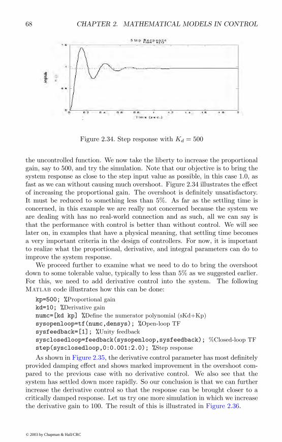
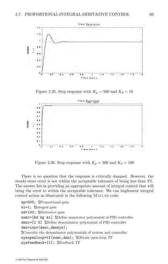
In this opening chapter, we present fundamental ideas of control theory throughsimple examples. These fundamental ideas apply no matter what mathematicalor engineering techniques are employed to solve the control problem. The exam-ples clearly identify the concepts underlying open-loop and closed-loop controlsystems. The need for feedback is recognized as an important component in con-trolling or regulating system performance. In the next chapter, we will presentexamples of classical modern control theory systems that rely on mathematicalmodels, and in the remainder of this book, we explore possible alternatives toa rigid mathematical model approach. These alternative approaches fuzzy,neural, and combinations of these provide alternative designs for autonomousintelligent control systems.

1.1 An ancient control system

Although modern control theory relies on mathematical models for its imple-mentation, control systems were invented long before mathematical tools wereavailable for developing such models. An amazing control system invented about2000 years ago by Hero of Alexandria, a device for the opening and closing oftemple doors is still viewed as a control system marvel. Figure 1.1 illustratesthe basic idea of his vision. The device was actuated whenever the ruler andhis entourage arrived to ascend the temple steps. The actuation consisted oflighting a Þre upon a sealed altar enclosing a column of air. As the air temper-ature in the sealed altar increased, the expanding hot air created airßow fromthe altar into a sealed vessel directly below. The increase in air pressure createdinside the vessel pushed out the water contained in this vessel. This water wascollected in a bucket. As the bucket became heavier, it descended and turnedthe door spindles by means of ropes, causing the counterweights to rise. The leftspindle rotated in the clockwise direction and the right spindle in the counter-

1

© 2003 by Chapman & Hall/CRC

2 CHAPTER 1. A PRELUDE TO CONTROL THEORY

Figure 1.1. Heros automatic temple doors

clockwise direction, thus opening the temple doors. The bucket, being heavierthan the counterweight, would keep the temple doors open as long as the Þreupon the altar was kept burning. Dousing the Þre with cold water caused thetemple doors to close.1 As the air in the altar cooled, the contracting cool airin the altar created a suction to extract hot air from the sealed vessel. Theresulting pressure drop caused the water from the bucket to be siphoned backinto the sealed vessel. Thus, the bucket became lighter, and the counterweight

1Here, there is a question on how slow or how fast the temple doors closed after dousingout the Þre. This is an important consideration, and a knowledge of the exponential decayin temperature of the air column inside the altar holds the answer. Naturally then, to give atheatrical appearance, Hero could have had copper tubes that carried the air column in closecontact with the heating and cooling surface. This would make the temperature rise quicklyat the time of opening the doors and drop quickly when closing the doors.


1.2. EXAMPLES OF CONTROL PROBLEMS 3

being heavier, moved down, thereby closing the door. This system was kept intotal secret, thus creating a mystic environment of superiority and power of theOlympian Gods and contributing to the success of the Greek Empire.

1.2 Examples of control problems

One goal of classical science is to understand the behavior of motion of physicalsystems. In control theory, rather than just to understand such behavior, theobject is to force a system to behave the way we want. Control is, roughlyspeaking, a means to force desired behaviors. The term control, as used here,refers generally to an instrument (possibly a human operator) or a set of instru-ments used to operate, regulate, or guide a machine or vehicle or some othersystem. The device that executes the control function is called the controller,and the system for which some property is to be controlled is called the plant.By a control system we mean the plant and the controller, together with the

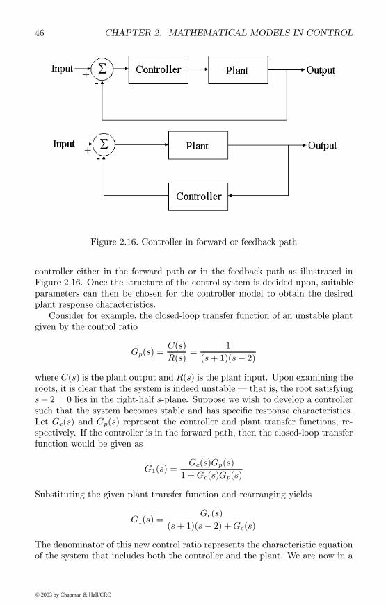
Figure 1.2. Control system

communication between them. The examples in this section include manual andautomatic control systems and combinations of these. Figure 1.2 illustrates thebasic components of a typical control system. The controlling device producesthe necessary input to the controlled system. The output of the controlled sys-tem, in the presence of unknown disturbances acting on the plant, acts as afeedback for the controlling device to generate the appropriate input.

1.2.1 Open-loop control systems

Consider a system that is driven by a human a car or a bicycle for example.If the human did not make observations of the environment, then it would beimpossible for the system to be controlled or driven in a safe and securemanner. Failure to observe the motion or movement of the system could havecatastrophic results. Stated alternatively, if there is no feedback regarding thesystems behavior, then the performance of the system is governed by how wellthe operator can maneuver the system without making any observations of thebehavior of the system. Control systems operating without feedback regardingthe systems behavior are known as open-loop control systems. In other



words, an open-loop control system is one where the control inputs are chosenwithout regard to the actual system outputs. The performance of such systemscan only be guaranteed if the task remains the same for all time and can beduplicated repeatedly by a speciÞc set of inputs.

Example 1.1 (Traffic light) To control the ßow of traffic on city streets, atraffic engineer may preset a Þxed time interval for a traffic light to turn green,yellow, and red. In this example, the environment around the street intersectionis the plant. Traffic engineers are interested in controlling some speciÞed plant

Figure 1.3. Traffic light, open-loop control

output, here the traffic ßow. The preset timer and on/off switch for the trafficlight comprise the controller. Since the traffic lights operate according to apreset interval of time, without taking into account the plant output (the timingis unaltered regardless of the traffic ßow), this control system is an open-loopcontrol system. A pictorial representation of the control design, called a blockdiagram, is shown in Figure 1.3.

Example 1.2 (Toaster) A toaster can be set for producing the desired dark-ness of toasted bread. The darkness setting allows a timer to time out andswitch off the power to the heating coils. The toaster is the plant, and the

Figure 1.4. Standard toaster

timing mechanism is the controller. The toaster by itself is unable to determinethe darkness of the toasted bread in order to adjust automatically the lengthof time that the coils are energized. Since the darkness of the toasted breaddoes not have any inßuence on the length of time heat is applied, there is nofeedback in such a system. This system, illustrated in Figure 1.4, is thereforean open-loop control system.

Example 1.3 (Automatic sprinkler system) An automatic home sprinklersystem is operated by presetting the times at which the sprinkler turns on andoff. The sprinkler system is the plant, and the automatic timer is the controller.



Figure 1.5. Automatic sprinkler system

There is no automatic feedback that allows the sprinkler system to modify thetimed sequence based on whether it is raining, or if the soil is dry or too wet.The block diagram in Figure 1.5 illustrates an open-loop control system.

Example 1.4 (Conventional oven) With most conventional ovens, the cook-ing time is prescribed by a human. Here, the oven is the plant and the controlleris the thermostat. By itself, the oven does not have any knowledge of the food

Figure 1.6. Conventional oven

condition, so it does not shut itself off when the food is done. This is, there-fore, an open-loop control system. Without human interaction the food wouldmost deÞnitely become inedible. This is typical of the outcome of almost allopen-loop control problems.

From the examples discussed in this section, it should become clear thatsome feedback is necessary in order for controllers to determine the amount ofcorrection, if any, needed to achieve a desired outcome. In the case of the toaster,for example, if an observation was made regarding the degree of darkness of thetoasted bread, then the timer could be adjusted so that the desired darknesscould be obtained. Similar observations can be made regarding the performanceof the controller in the other examples discussed.

1.2.2 Closed-loop control systems

Closed-loop systems, or feedback control systems, are systems where thebehavior of the system is observed by some sensory device, and the observationsare fed back so that a comparison can be made about how well the system isbehaving in relation to some desired performance. Such comparisons of theperformance allow the system to be controlled or maneuvered to the desiredÞnal state. The fundamental objective in closed-loop systems is to make theactual response of a system equal to the desired response.



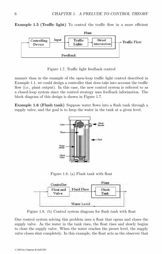
Example 1.5 (Traffic light) To control the traffic ßow in a more efficient

Figure 1.7. Traffic light feedback control

manner than in the example of the open-loop traffic light control described inExample 1.1, we could design a controller that does take into account the trafficßow (i.e., plant output). In this case, the new control system is referred to asa closed-loop system since the control strategy uses feedback information. Theblock diagram of this design is shown in Figure 1.7.

Example 1.6 (Flush tank) Suppose water ßows into a ßush tank through asupply valve, and the goal is to keep the water in the tank at a given level.

Figure 1.8. (a) Flush tank with ßoat

Figure 1.8. (b) Control system diagram for ßush tank with ßoat

One control system solving this problem uses a ßoat that opens and closes thesupply valve. As the water in the tank rises, the ßoat rises and slowly beginsto close the supply valve. When the water reaches the preset level, the supplyvalve closes shut completely. In this example, the ßoat acts as the observer that



provides feedback regarding the water level. This feedback is compared withthe desired level, which is the Þnal position of the ßoat (see Figures 1.8 (a) and(b)).

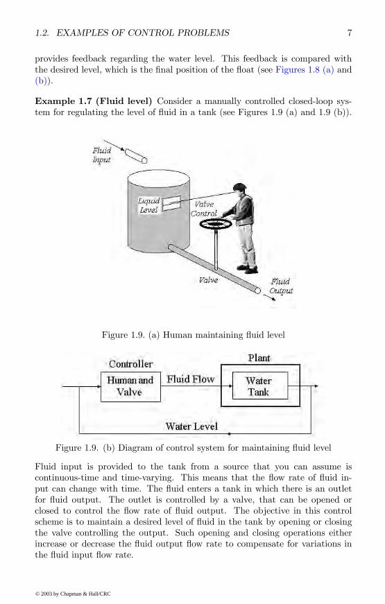
Example 1.7 (Fluid level) Consider a manually controlled closed-loop sys-tem for regulating the level of ßuid in a tank (see Figures 1.9 (a) and 1.9 (b)).

Figure 1.9. (a) Human maintaining ßuid level

Figure 1.9. (b) Diagram of control system for maintaining ßuid level

Fluid input is provided to the tank from a source that you can assume iscontinuous-time and time-varying. This means that the ßow rate of ßuid in-put can change with time. The ßuid enters a tank in which there is an outletfor ßuid output. The outlet is controlled by a valve, that can be opened orclosed to control the ßow rate of ßuid output. The objective in this controlscheme is to maintain a desired level of ßuid in the tank by opening or closingthe valve controlling the output. Such opening and closing operations eitherincrease or decrease the ßuid output ßow rate to compensate for variations inthe ßuid input ßow rate.



The operator is instructed to maintain the level of ßuid in the tank at aparticular level. A porthole on the side of the tank provides the operator awindow to observe the ßuid level. A reference marker is placed in the windowfor the operator to see exactly where the ßuid level should be. If the ßuid leveldrops below the reference marker, the human sees the ßuid level and comparesit with the reference. Sensing whether the height of ßuid is above or belowthe reference, the operator can turn the valve either in the clockwise (close) orcounterclockwise (open) direction and control the ßow rate of the ßuid outputfrom the tank.Good feedback control action can be achieved if the operator can contin-

uously adjust the valve position. This will ensure that the error between thereference marker position, and the actual height of ßuid in the tank, is kept toa minimum. The controller in this example is a human operator together withthe valve system. As a component of the feedback system, the human operatoris performing two tasks, namely, sensing the actual height of ßuid and compar-ing the reference with the actual ßuid height. Feedback comes from the visualsensing of the actual position of the ßuid in the tank.

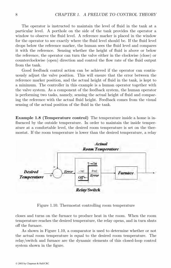
Example 1.8 (Temperature control) The temperature inside a home is in-ßuenced by the outside temperature. In order to maintain the inside temper-ature at a comfortable level, the desired room temperature is set on the ther-mostat. If the room temperature is lower than the desired temperature, a relay

Figure 1.10. Thermostat controlling room temperature

closes and turns on the furnace to produce heat in the room. When the roomtemperature reaches the desired temperature, the relay opens, and in turn shutsoff the furnace.As shown in Figure 1.10, a comparator is used to determine whether or not

the actual room temperature is equal to the desired room temperature. Therelay/switch and furnace are the dynamic elements of this closed-loop controlsystem shown in the Þgure.


1.3. STABLE AND UNSTABLE SYSTEMS 9

1.3 Stable and unstable systemsStability of an uncontrolled system indicates resistance to change, deterioration,or displacement, in particular the ability of the system to maintain equilibriumor resume its original position after displacement. Any system that violatesthese characteristics is unstable. A closed-loop system must, aside from meetingperformance criteria, be stable.

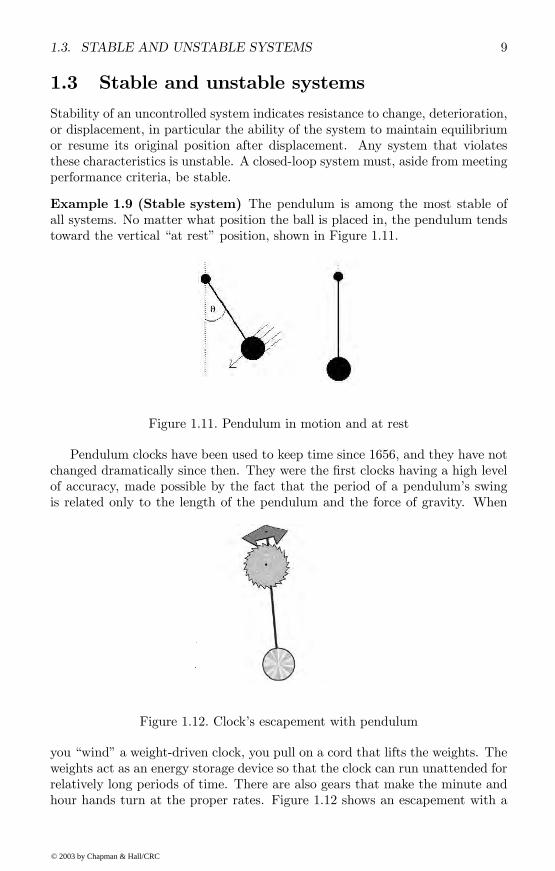
Example 1.9 (Stable system) The pendulum is among the most stable ofall systems. No matter what position the ball is placed in, the pendulum tendstoward the vertical at rest position, shown in Figure 1.11.

Figure 1.11. Pendulum in motion and at rest

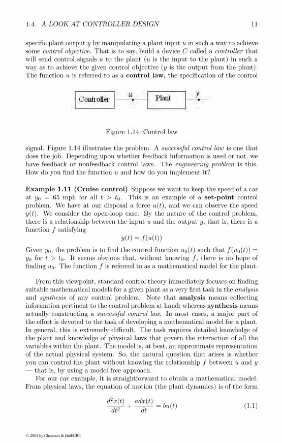
Pendulum clocks have been used to keep time since 1656, and they have notchanged dramatically since then. They were the Þrst clocks having a high levelof accuracy, made possible by the fact that the period of a pendulums swingis related only to the length of the pendulum and the force of gravity. When

Figure 1.12. Clocks escapement with pendulum

you wind a weight-driven clock, you pull on a cord that lifts the weights. Theweights act as an energy storage device so that the clock can run unattended forrelatively long periods of time. There are also gears that make the minute andhour hands turn at the proper rates. Figure 1.12 shows an escapement with a



gear having teeth of a special shape. Attached to the pendulum is a device toengage the teeth of the gear. For each swing of the pendulum, one tooth of thegear is allowed to escape. That is what produces the ticking sound of a clock.One additional job of the escapement gear is to impart just enough energy intothe pendulum to overcome friction and allow it to keep swinging.

Example 1.10 (Unstable system) An inverted pendulum is an uprightpole with its fulcrum at the base. The objective is to balance the pole in theupright position by applying the appropriate force at the base. An invertedpendulum is inherently unstable, as you can observe by trying to balance a poleupright in your hand (Figure 1.13). Feedback control can be used to stabilizean inverted pendulum. We will give several examples in later chapters.

Figure 1.13. Balancing inverted pendulum

1.4 A look at controller designSynthesizing the above examples of control problems, we can describe a typicalcontrol problem as follows. For a given plant P , it is desirable to control a


1.4. A LOOK AT CONTROLLER DESIGN 11

speciÞc plant output y by manipulating a plant input u in such a way to achievesome control objective. That is to say, build a device C called a controller thatwill send control signals u to the plant (u is the input to the plant) in such away as to achieve the given control objective (y is the output from the plant).The function u is referred to as a control law, the speciÞcation of the control

Figure 1.14. Control law

signal. Figure 1.14 illustrates the problem. A successful control law is one thatdoes the job. Depending upon whether feedback information is used or not, wehave feedback or nonfeedback control laws. The engineering problem is this.How do you Þnd the function u and how do you implement it?

Example 1.11 (Cruise control) Suppose we want to keep the speed of a carat y0 = 65 mph for all t > t0. This is an example of a set-point controlproblem. We have at our disposal a force u(t), and we can observe the speedy(t). We consider the open-loop case. By the nature of the control problem,there is a relationship between the input u and the output y, that is, there is afunction f satisfying

y(t) = f(u(t))

Given y0, the problem is to Þnd the control function u0(t) such that f(u0(t)) =y0 for t > t0. It seems obvious that, without knowing f , there is no hope ofÞnding u0. The function f is referred to as a mathematical model for the plant.

From this viewpoint, standard control theory immediately focuses on Þndingsuitable mathematical models for a given plant as a very Þrst task in the analysisand synthesis of any control problem. Note that analysis means collectinginformation pertinent to the control problem at hand; whereas synthesismeansactually constructing a successful control law. In most cases, a major part ofthe effort is devoted to the task of developing a mathematical model for a plant.In general, this is extremely difficult. The task requires detailed knowledge ofthe plant and knowledge of physical laws that govern the interaction of all thevariables within the plant. The model is, at best, an approximate representationof the actual physical system. So, the natural question that arises is whetheryou can control the plant without knowing the relationship f between u and y that is, by using a model-free approach.For our car example, it is straightforward to obtain a mathematical model.

From physical laws, the equation of motion (the plant dynamics) is of the form

d2x(t)

dt2+adx(t)

dt= bu(t) (1.1)



where x(t) denotes the cars position.The velocity is described by the equation y(t) = dx(t)/dt, so Equation 1.1,

written in terms of y, isdy(t)

dt+ ay(t) = bu(t) (1.2)

This equation gives rise to the needed relation between the input u(t) and outputy(t), namely y(t) = f(u(t)). This is done by solving for u(t) for a given y(t).This equation itself provides the control law immediately. Indeed, from it yousee that, in order for y(t) = y0, for t > 0, the acceleration dy(t)/dt should beequal to zero, so it is sufficient to take u(t) = (a/b)y0 for all t > 0.To solve the second-order linear differential equation in Equation 1.2, you

can use Laplace transforms. This yields the transfer function F (s) of theplant and puts you in the frequency domain that is, you are workingwith functions of the complex frequency s. Taking inverse Laplace transformsreturns u(t), putting you back in the time domain. These transformationsoften simplify the mathematics involved and also expose signiÞcant componentsof the equations. You will see some examples of this in Chapter 2. Note that thisexample is not realistic for implementation, but it does illustrate the standardcontrol approach.The point is that to obtain a control law analytically, you need a mathemati-

cal model for the plant. This might imply that if you dont have a mathematicalmodel for your plant, you cannot Þnd a control law analytically. So, how canyou control complicated systems whose plant dynamics are difficult to know?A mathematical model may not be a necessary prerequisite for obtaining a suc-cessful control law. This is precisely the philosophy of the fuzzy and neuralapproaches to control.To be precise, typically, as in several of the preceding examples, feedback

control is needed for a successful system. These closed-loop controls are closelyrelated to the heuristics of If...then... rules. Indeed, if you feed back the plantoutput y(t) to the controller, then the control u(t) should be such that the errory(t)− y0 = e(t) goes to zero. So, apparently, the design of the control law u(t)is reduced to another box with input e(t) and output u(t). Thus,

u(t) = g(e(t)) = h(y(t), y0)

The problem is to Þnd the function g or to approximate it from observablevalues of u(t) and y(t). Even though y(t) comes out from the plant, you dontneed the plants mathematical model to be able to observe y(t). Thus, wheredoes the mathematical model of the plant come to play in standard controltheory, in the context of feedback control? From a common-sense viewpoint,we can often suggest various obvious functions g. This is done for the so-calledproportional integral derivative (PID) types of controllers discussed in the nextchapter. However, these controllers are not automatically successful controllers.Just knowing the forms of these controllers is not sufficient information to makethem successful. Choosing good parameters in these controllers is a difficultdesign problem, and it is precisely here that the mathematical model is needed.


1.4. A LOOK AT CONTROLLER DESIGN 13

In the case of linear and time-invariant systems, the mathematical model canbe converted to the so-called transfer functions of the plant and of the controllerto be designed. As we will see, knowledge of the poles of these transfer functionsis necessary for designing state-variable feedback controllers or PID controllersthat will perform satisfactorily.

Even for linear and time-invariant plants, the modern view of control isfeedback control. From that viewpoint, a control law is a function of the error.Proposing a control law, or approximating it from training data (a curve Þttingproblem), are obvious ways to proceed. The important point to note is thatthe possible forms of a control law are not derived from a mathematical modelof the plant, but rather from heuristics. What the mathematical model does ishelp in a systematic analysis leading to the choice of good parameters in theproposed control law, in order to achieve desirable control properties. In otherwords, with a mathematical model for the plant, there exist systematic ways todesign successful controllers.

In the absence of a mathematical model for the plant, we can always approx-imate a plausible control law, either from a collection of If. . . then. . . rules orfrom training data. When we construct a control law by any approximationprocedures, however, we have to obtain a good approximation. There are noparameters, per se, in this approximation approach to designing control laws.There are of course parameters in weights of neural networks, or in the mem-bership functions used by fuzzy rules, but they will be adjusted by trainingsamples or trial and error. There is no need for analytical mathematical modelsin this process. Perhaps that is the crucial point explaining the success of softcomputing approaches to control.

Let us examine a little more closely the prerequisite for mathematical models.First, even in the search for a suitable mathematical model for the plant, wecan only obtain, in most cases, a mathematical representation that approximatesthe plant dynamics. Second, from a common sense point of view, any controlstrategy is really based upon If. . . then. . . rules. The knowledge of a functionalrelationship f provides speciÞc If. . . then. . . rules, often more than needed.The question is: Can we Þnd control laws based solely on If. . . then. . . rules?If yes, then obviously we can avoid the tremendous task of spending the majorpart of our effort in Þnding a mathematical model. Of course, if a suitablemathematical model is readily available, we generally should use it.

Our point of view is that a weaker form of knowledge, namely a collectionof If...then... rules, might be sufficient for synthesizing control laws. Therationale is simple: we are seeking an approximation to the control law that is, the relationship between input and output of the controller directly,and not the plant model. We are truly talking about approximating functions.The many ways of approximating an unknown function include using trainingsamples (neural networks) and linguistic If. . . then. . . rules (fuzzy logic).2

2 In both cases, the theoretical foundation is the so-called universal approximation capabil-ity, based on the Stone-Weierstrass Theorem, leading to good models for control laws.



In summary, standard control theory emphasizes the absolute need to havea suitable mathematical model for the plant in order to construct successfulcontrol laws. Recognizing that in formulating a control law we might onlyneed weaker knowledge, neural and fuzzy control become useful alternatives insituations where mathematical models of plants are hard to specify.

1.5 Exercises and projects1. In Heros ancient control system, identify the controller and the plant.Develop a block diagram and label various plant details.

2. For the examples shown for open-loop systems, how would you modifyeach system to provide closed-loop control? Explain with the help ofblock diagrams both open- and closed-loop systems for each example.

3. The Intelligent Vehicle Highway System (IVHS) program for future trans-portation systems suggests the possibility of using sensors and controllersto slow down vehicles automatically near hospitals, accident locations, andconstruction zones. If you were to design a system to control the ßow oftraffic in speed-restricted areas, what are the major considerations youhave to consider, knowing that the highway system is the controller andthe vehicle is the plant? Draw a block diagram that illustrates your designconcept. Explain the workings of the IVHS system design.

4. A moving sidewalk is typically encountered in large international airports.Design a moving sidewalk that operates only when a passenger approachesthe sidewalk and stops if there are no passengers on, or approaching,the sidewalk. Discuss what type of sensors might be used to detect theapproach of passengers, and the presence of passengers on the sidewalk.

5. A baggage handling system is to be designed for a large internationalairport. Baggage typically comes off a conveyor and slides onto a carouselthat goes around and around. The objective here is to prevent one bagfrom sliding onto another bag causing a pile up. Your task is to design asystem that allows a bag to slide onto the carousel only if there is roombetween two bags, or if there are no bags. Explain your system with theaid of a block diagram of the control system.

6. A soda bottling plant requires sensors to detect if bottles have the rightamount of soda and a metal cap. With the aid of sketches and blockdiagrams, discuss in detail how you would implement a system of sensorsto detect soda level in the bottles and whether or not there is a metal capon each bottle of soda. State all your assumptions in choosing the type ofsensor(s) you wish to use.

7. A potato chip manufacturing plant has to package chips with each bag ofchips having a net weight of 16 ounces or 453.6 grams. Discuss in detailhow a system can be developed that will guarantee the desired net weight.


Chapter 2

MATHEMATICALMODELS IN CONTROL

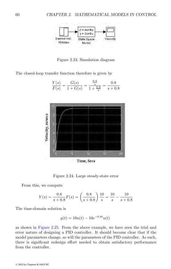
In this chapter we present the basic properties of control and highlight signiÞcantdesign and operating criteria of model-based control theory. We discuss theseproperties in the context of two very popular classical methods of control: state-variable feedback control, and proportional-integral-derivative (PID) control.This chapter serves as a platform for discussing the desirable properties of acontrol system in the context of fuzzy and neural control in subsequent chapters.It is not our intent to present a thorough treatment of classical control theory,but rather, to present relevant material that provides the foundations for fuzzyand neural control systems. The reader therefore is urged to refer to the manyexcellent sources in classical control theory for further information.Standard control theory consists of two tasks, analysis and synthesis. Analy-

sis refers to the study of the plant and the control objectives. Synthesis refersto designing and building the controller to achieve the objectives. In standardcontrol theory, mathematical models are used in both the analysis and the syn-thesis of controllers.

2.1 Introductory examples: pendulum problems

We present two simple, but detailed, examples to bring out the general frame-work and techniques of standard control theory. The Þrst is a simple pendulum,Þxed at one end, controlled by a rotary force; and the second is an invertedpendulum with one end on a moving cart. The concepts introduced in these ex-amples are all discussed more formally, and in more detail, later in this chapter.

2.1.1 Example: Þxed pendulum

We choose the problem of controlling a pendulum to provide an overview ofstandard control techniques, following the analysis in [70]. In its simpliÞed

15


16 CHAPTER 2. MATHEMATICAL MODELS IN CONTROL

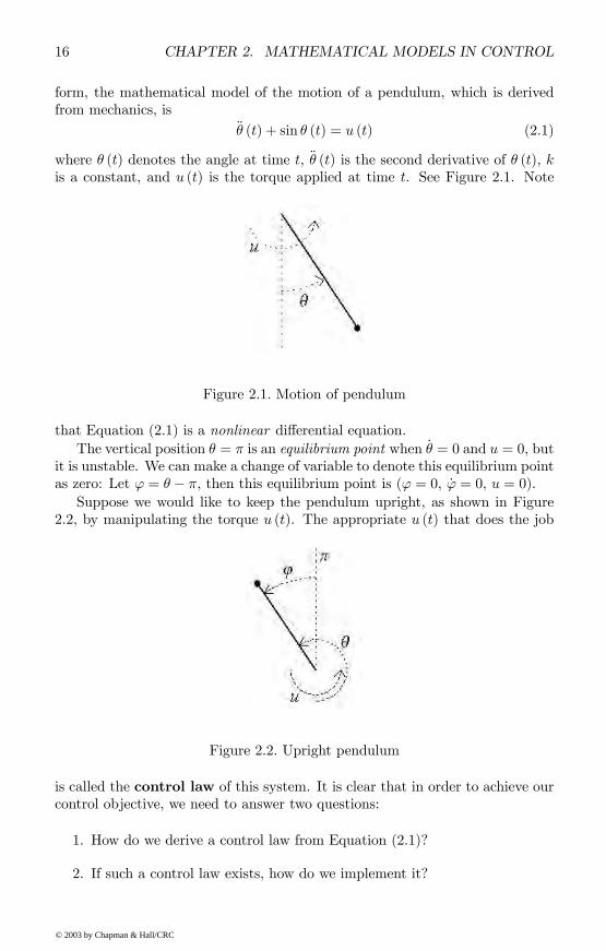
form, the mathematical model of the motion of a pendulum, which is derivedfrom mechanics, is

θ (t) + sin θ (t) = u (t) (2.1)

where θ (t) denotes the angle at time t, θ (t) is the second derivative of θ (t), kis a constant, and u (t) is the torque applied at time t. See Figure 2.1. Note

Figure 2.1. Motion of pendulum

that Equation (2.1) is a nonlinear differential equation.The vertical position θ = π is an equilibrium point when úθ = 0 and u = 0, but

it is unstable. We can make a change of variable to denote this equilibrium pointas zero: Let ϕ = θ − π, then this equilibrium point is (ϕ = 0, úϕ = 0, u = 0).Suppose we would like to keep the pendulum upright, as shown in Figure

2.2, by manipulating the torque u (t). The appropriate u (t) that does the job

Figure 2.2. Upright pendulum

is called the control law of this system. It is clear that in order to achieve ourcontrol objective, we need to answer two questions:

1. How do we derive a control law from Equation (2.1)?

2. If such a control law exists, how do we implement it?


2.1. INTRODUCTORY EXAMPLES: PENDULUM PROBLEMS 17

In this example, we concentrate on answering the Þrst question. When weattempt to keep the pendulum upright, our operating range is a small rangearound the unstable equilibrium position. As such, we have a local controlproblem, and we can simplify the mathematical model in Equation (2.1) bylinearizing it around the equilibrium point. For ϕ = θ − π small, we keep onlythe Þrst-order term in the Taylor expansion of sin θ, that is, − (θ − π), so thatthe linearization of Equation (2.1) is the linear model (the linear differentialequation)

ϕ (t)− ϕ (t) = u (t) (2.2)

and the control objective is manipulating u (t) to bring ϕ (t) and úϕ (t) to zerofrom any small nonzero initial ϕ (0), úϕ (0).Note that Equation (2.2) is a second-order differential equation. It is conve-

nient to replace Equation (2.2) by a system of Þrst-order differential equationsin terms of ϕ (t) and úϕ (t). Here, let x (t) be the vector

x (t) =

µx1 (t)x2 (t)

¶=

µϕ (t)úϕ (t)

¶so that

úx (t) =

µúϕ (t)ϕ (t)

¶=

µx2 (t)úx2 (t)

¶With this notation we see that the original model, Equation (2.1), is written as

úx = f (x, u) (2.3)

where f is nonlinear, and

f =

µf1f2

¶where f1 (x, u) = x2 and f2 (x, u) = − sin (x1 + π) + u. Since f is continuouslydifferentiable and f (0, 0) = 0, we can linearize f around (x, u) = (0, 0) as

úx = Ax+Bu (2.4)

where the matrices A and B are

A =

Ã∂f1∂x1

∂f1∂x2

∂f2∂x1

∂f2∂x2

!=

µ0 11 0

¶

B =

Ã∂f1∂u∂f2∂u

!=

µ01

¶with both Jacobian matrices A and B evaluated at (x, u) = (0, 0).Thus, in the state-space representation, Equation (2.2) is replaced by Equa-

tion (2.4). Note that, in general, systems of the form (2.4) are called linearsystems, and when A and B do not depend on time, they are called time-invariant systems.



Now back to our control problem. Having simpliÞed the original dynamics,Equation (2.1) to the nicer form of Equation (2.2), we are now ready for theanalysis leading to the derivation of a control law u (t). The strategy is this.By examining the system under consideration and our control objective, theform of u (t) can be suggested by common sense or naive physics. Then themathematical model given by Equation (2.2) is used to determine (partially)the control law u (t).In our control example, u (t) can be suggested from the following heuristic

If .. then ... rules:

If ϕ is positive, then u should be negativeIf ϕ is negative, then u should be positive

From these common sense rules, we can conclude that u (t) should be of theform

u (t) = −αϕ (t) (2.5)

for some α > 0. A control law of the form (2.5) is called a proportionalcontrol law, and α is called the feedback gain. Note that (2.5) is a feedbackcontrol since it is a function of ϕ (t).To obtain u (t), we need α and ϕ (t). In implementation, with an appropriate

gain α, u (t) is determined since ϕ (t) can be measured directly by a sensor. Butbefore that, how do we know that such a control law will stabilize the invertedpendulum? To answer this, we substitute Equation (2.5) into Equation (2.2),resulting in the equation

ϕ (t)− ϕ (t) + αϕ (t) = 0 (2.6)

In a sense, this is analogous to guessing the root of an equation and checkingwhether it is indeed a root. Here, in control context, checking that u (t) issatisfactory or not amounts to checking if the solution ϕ (t) of Equation (2.6)converges to 0 as t → +∞, that is, checking whether the controller will sta-bilize the system. This is referred to as the control system (the plant and thecontroller) being asymptotically stable.For this purpose, we have, at our disposal, the theory of stability of linear

differential equations. Thus, we examine the characteristic equation of (2.6),namely

z2 + α− 1 = 0 (2.7)

For α > 1, the roots of (2.7) are purely imaginary: z = ± j√α− 1, wherej =

√−1. As such, the solutions of (2.6) are all oscillatory and hence do notconverge to zero. For α ≤ 1, it can also be seen that ϕ (t) does not converge tozero as t→ +∞. Thus, u (t) = −αϕ (t) is not a good guess.Let us take another guess. By closely examining why the proportional control

does not work, we propose to modify it as follows. Only for α > 1 do we havehope to modify u (t) successfully. In this case, the torque is applied in the correctdirection, but at the same time it creates more inertia, resulting in oscillationsof the pendulum. Thus, it appears we need to add to u (t) something that acts



like a brake. In technical terms, we need to add damping to the system. ThemodiÞed control law is now

u (t) = −αϕ (t)− β úϕ (t) (2.8)

for α > 1 and β > 0. Because of the second term in u (t), these types of controllaws are called proportional-derivative (feedback) control laws, or simply PDcontrol.To determine if Equation (2.8) is a good guess, as before, we look at the

characteristic equationz2 + βz + α− 1 = 0 (2.9)

of the closed-loop, second-order linear differential equation

ϕ (t) + β úϕ (t) + (α− 1)ϕ (t) = 0 (2.10)

For α > 1 and β > 0, the roots of Equation (2.9) are

z =−β ±

qβ2 − 4 (α− 1)2

and hence both have negative real parts. Basic theorems in classical controltheory then imply that all solutions of Equation (2.2) with this control law willconverge to zero as t gets large. In other words, the PD control laws will do thejob. In practice, suitable choices of α and β are needed to implement a goodcontroller. Besides α and β, we need the value úϕ (t), in addition to ϕ (t), inorder to implement u (t) by Equation (2.8).Suppose we can only measure ϕ (t) but not úϕ (t), that is, our measurement

of the state

x (t) =

µϕ (t)úϕ (t)

¶is of the form

y (t) = Cx (t) (2.11)

for some known matrix C. Here, C =¡1 0

¢.

Equation (2.11) is called the measurement (or output) equation, that,in general, is part of the speciÞcation of a control problem (together with (2.4)in the state-space representation).In a case such as the above, a linear feedback control law that depends only

on the allowed measurements is of the form

u (t) = KCx (t)

Of course, to implement u (t), we need to estimate the components of x (t) thatare not directly measured, for example úϕ (t), by some procedures. A control lawobtained this way is called a dynamic controller.At this point, it should be mentioned that u and y are referred to as input

and output, respectively. Approximating a system from input-output observeddata is called system identiÞcation.



Let us further pursue our problem of controlling an inverted pendulum. Thelinearized model in Equation (2.2) could be perturbed by some disturbance e,say, resulting in

ϕ (t)− ϕ (t) = u (t) + e (2.12)

To see if our PD control law is sufficient to handle this new situation, weput (2.8) into (2.12), resulting in

ϕ (t) + β úϕ (t) + (α− 1)ϕ (t) = e (2.13)

and examine the behavior of the solutions of (2.13) for t large. It can be shown,unfortunately, that no solutions of (2.13) converge to zero as t → +∞. So weneed to modify (2.8) further to arrive at an acceptable control law. Withoutgoing into details here (but see examples in Section 2.7), the additional term toadd to our previous PD control law is of the form

−γZ t

0

ϕ (s) ds

This term is used to offset a nonzero error in the PD control. Thus, our newcontrol law takes the form

u (t) = −αϕ (t)− β úϕ (t)− γZ t

0

ϕ (s) ds (2.14)

A control law of the form (2.14) is called a proportional-integral-derivative(PID) control. PID control is very popular in designing controllers for linear sys-tems. It is important to note that, while PID controls are derived heuristically,stability analysis requires the existence of mathematical models of the dynamicsof the systems, and stability analysis is crucial for designing controllers.In our control example, we started out with a nonlinear system. But since

our control objective was local in nature, we were able to linearize the system andthen apply powerful techniques in linear systems. For global control problems,as well as for highly nonlinear systems, one should look for nonlinear controlmethods. In view of the complex behaviors of nonlinear systems, there are nosystematic tools and procedures for designing nonlinear control systems. Theexisting design tools are applicable to particular classes of control problems.However, stability analysis of nonlinear systems can be based on Lyapunovsstability theory.

2.1.2 Example: inverted pendulum on a cart

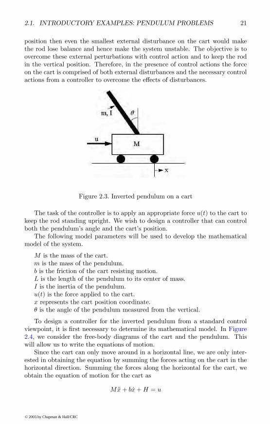
We look at a standard approach for controlling an inverted pendulum, which wewill contrast later with fuzzy control methods. The following mechanical systemis referred to as an inverted pendulum system. In this system, illustratedin Figure 2.3, a rod is hinged on top of a cart. The cart is free to move in thehorizontal plane, and the objective is to balance the rod in the vertical position.Without any control actions on the cart, if the rod were initially in the vertical



position then even the smallest external disturbance on the cart would makethe rod lose balance and hence make the system unstable. The objective is toovercome these external perturbations with control action and to keep the rodin the vertical position. Therefore, in the presence of control actions the forceon the cart is comprised of both external disturbances and the necessary controlactions from a controller to overcome the effects of disturbances.

Figure 2.3. Inverted pendulum on a cart

The task of the controller is to apply an appropriate force u(t) to the cart tokeep the rod standing upright. We wish to design a controller that can controlboth the pendulums angle and the carts position.The following model parameters will be used to develop the mathematical

model of the system.

M is the mass of the cart.m is the mass of the pendulum.b is the friction of the cart resisting motion.L is the length of the pendulum to its center of mass.I is the inertia of the pendulum.u(t) is the force applied to the cart.x represents the cart position coordinate.θ is the angle of the pendulum measured from the vertical.

To design a controller for the inverted pendulum from a standard controlviewpoint, it is Þrst necessary to determine its mathematical model. In Figure2.4, we consider the free-body diagrams of the cart and the pendulum. Thiswill allow us to write the equations of motion.Since the cart can only move around in a horizontal line, we are only inter-

ested in obtaining the equation by summing the forces acting on the cart in thehorizontal direction. Summing the forces along the horizontal for the cart, weobtain the equation of motion for the cart as

Mx+ b úx+H = u



Figure 2.4. Free-body diagrams of the cart and the pendulum

By summing the forces along the horizontal for the pendulum, we get the fol-lowing equation of motion:

H = mx+mLθ cos θ −mL úθ2 sin θSubstituting this equation into the equation of motion for the cart and collectingterms gives

(M +m)x+ b úx+mLθ cos θ −mL úθ2 sin θ = u (2.15)

This is the Þrst of two equations needed for a mathematical model.The second equation of motion is obtained by summing all the forces in the

vertical direction for the pendulum. Note that, as we pointed out earlier, weonly need to consider the horizontal motion of the cart; and as such, there is nouseful information we can obtain by summing the vertical forces for the cart.By summing all the forces in the vertical direction acting on the pendulum, weobtain

V sin θ +H cos θ −mg sin θ = mLθ +mx cos θIn order to eliminate the H and V terms, we sum the moments around the

centroid of the pendulum to obtain

−V L sin θ −HL cos θ = IθSubstituting this in the previous equation and collecting terms yields

(mL2 + I)θ +mgL sin θ = −mLx cos θ (2.16)

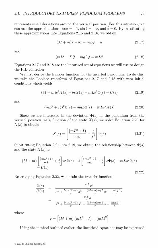
Equations 2.15 and 2.16 are the equations of motion describing the nonlinearbehavior of the inverted pendulum. Since our objective is to design a controllerfor this nonlinear problem, it is necessary for us to linearize this set of equations.Our goal is to linearize the equations for values of θ around π, where θ = π isthe vertical position of the pendulum. Consider values of θ = π + ϕ where ϕ



represents small deviations around the vertical position. For this situation, wecan use the approximations cos θ = −1, sin θ = −ϕ, and θ = 0. By substitutingthese approximations into Equations 2.15 and 2.16, we obtain

(M +m)x+ b úx−mLϕ = u (2.17)

and

(mL2 + I)ϕ−mgLϕ = mLx (2.18)

Equations 2.17 and 2.18 are the linearized set of equations we will use to designthe PID controller.We Þrst derive the transfer function for the inverted pendulum. To do this,

we take the Laplace transform of Equations 2.17 and 2.18 with zero initialconditions which yields

(M +m)s2X(s) + bsX(s)−mLs2Φ(s) = U(s) (2.19)

and

(mL2 + I)s2Φ(s)−mgLΦ(s) = mLs2X(s) (2.20)

Since we are interested in the deviation Φ(s) in the pendulum from thevertical position, as a function of the state X(s), we solve Equation 2.20 forX(s) to obtain

X(s) =

"¡mL2 + I

¢mL

− g

s2

#Φ(s) (2.21)

Substituting Equation 2.21 into 2.19, we obtain the relationship between Φ(s)and the state X(s) as

(M +m)

·(mL2+I)

mL + gs

¸s2Φ(s) + b

·(mL2+I)

mL + gs

¸sΦ(s)−mLs2Φ(s)

= U(s)(2.22)

Rearranging Equation 2.22, we obtain the transfer function

Φ(s)

U(s)=

mLr s

2

s4 + b(mL2+I)r s3 − (M+m)mgL

r s2 − bmgLr s

=mLr s

s3 + b(mL2+I)r s2 − (M+m)mgL

r s− bmgLr

where

r =h(M +m)

¡mL2 + I

¢− (mL)2iUsing the method outlined earlier, the linearized equations may be expressed



in state-space form asúx1(t)úx2(t)úϕ1(t)úϕ2(t)

=

0 1 0 0

0−(mL2+I)b

(M+m)I+MmL2m2gL2

(M+m)I+MmL2 0

0 0 0 1

0 −mLb(M+m)I+MmL2

mgL(M+m)(M+m)I+MmL2 0

x1(t)x2(t)ϕ1(t)ϕ2(t)

+

0

(mL2+I)(M+m)I+MmL2

0mL

(M+m)I+MmL2

u (t)where úx1(t) = úx, úx2(t) = x, úϕ1(t) = úϕ and úϕ2(t) = ϕ. Since we are interestedin the position of the cart, as well as the angular position of the pendulum, theoutput may be synthesized as

·y1(t)y2(t)

¸=

·1 0 0 00 0 1 0

¸x1(t)x2(t)ϕ1(t)ϕ2(t)

+ · 00¸u (t)

For this example we will assume the following parameters:

M = 0.5 kg

m = 0.2 kg

b = 0.1N/m/ s

l = 0.3m

I = 0.006 kgm2

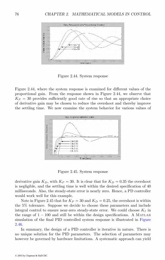
To make the design more challenging, we will be applying a step input to thecart. The cart should achieve its desired position within 5 seconds and have arise time under 0.5 seconds. We will also limit the pendulums overshoot to 20degrees (0.35 radians), and it should also settle in under 5 seconds. The designrequirements for the inverted pendulum are therefore

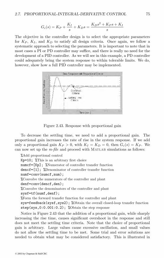
settling time for x and θ of less than 5 seconds, rise time for x of less than 0.5 seconds, and overshoot of θ less than 20 degrees (0.35 radians).

We use Matlab to perform several computations. First, we wish to obtain thetransfer function for the given set of parameters. Using the m-Þle shown below,we can obtain the coefficients of the numerator and denominator polynomials.M = .5;m = 0.2;



b = 0.1;i = 0.006;g = 9.8;l = 0.3;r = (M+m)*(i+m*l*l)-(m*l)*(m*l);numplant = [m*l/q 0];denplant = [1 b*(i+m*l^2)/q -(M+m)*m*g*l/q -b*m*g*l/q];

The coefficients of the numerator and denominator polynomial from theMatlab output can be translated to the following plant transfer function:

Gp(s) =4.5455

s3 + 0.1818s2 − 31.1818s− 4.4545 =Np(s)

Dp(s)

The open-loop response of this transfer function can be simulated in Matlabusing the following code:t = 0:0.01:5;impulse(numplant,denplant,t)axis([0 0.9 0 60]);

The plot shown in Figure 2.5 clearly indicates the unstable nature of theplant in an open-loop setup.

Figure 2.5. Unstable plant

We can now extend the Matlab script Þle to include computation of thestate-space model. The necessary code is as follows:p = i*(M+m)+M*m*l*l;A = [0 1 0 0;0 -(i+m*l*l)*b/p (m*m*g*l*l)/p 0;0 0 0 1;0 -(m*l*b)/p m*g*l*(M+m)/p 0]B = [ 0;(i+m*l*l)/p;0;m*l/p]



C = [1 0 0 0;0 0 1 0]D = [0;0]

The output gives the following state-space modelúx1(t)úx2(t)úϕ1(t)úϕ2(t)

=0 1 0 00 −0.1818 2.6727 00 0 0 10 −0.4545 31.1818 0

x1(t)x2(t)ϕ1(t)ϕ2(t)

+

01.81820

4.5455

u (t)·y1(t)y2(t)

¸=

·1 0 0 00 0 1 0

¸x1(t)x2(t)ϕ1(t)ϕ2(t)

+ · 00¸u (t)

Figure 2.6. Time simulation for a unit step

Figure 2.7. Original control structure

Figure 2.6 shows the response of the open-loop system where the systemis unstable and Figure 2.7 illustrates the closed-loop control structure for thisproblem. Note that the control objective is to bring the pendulum to the uprightposition. As such, the output of the plant is tracking a zero reference with the



vertical reference set to a zero value. Hence, the control structure may beredrawn as shown in Figure 2.8. The force applied to the cart is added as animpulse disturbance.

Figure 2.8. ModiÞed control structure

From the modiÞed control structure, we can obtain the closed-loop transferfunction that relates the output with the disturbance input. Referring to Figure2.8,

E(s) = D(s)−Gc(s)Y (s)and

Y (s) = Gp(s)E(s)

Therefore,Y (s)

D(s)=

Gp(s)

[1 +Gp(s)Gc(s)]

DeÞning the transfer function of the PID controller

Gc(s) =Nc(s)

Dc(s)

and using

Gp(s) =Np(s)

Dp(s)

we can write the transfer function as

Y (s)

D(s)=

Np(s)Dp(s)

[1 + Nc(s)Dc(s)

Np(s)Dp(s)

]=

Np(s)Dc(s)

[Dc(s)Dp(s) +Nc(s)Np(s)]

Since the transfer function for the PID controller is

Gc(s) =

¡s2KD + sKP +KI

¢s

=Nc(s)

Dc(s)

and the transfer function of the inverted pendulum with a cart is

Gp(s) =4.5455

s3 + 0.1818s2 − 31.1818s− 4.4545 =Np(s)

Dp(s)



we can easily manipulate the transfer function inMatlab for various numericalvalues of KP , KD, and KI . To convolve the polynomials in the denominator ofthe transfer function, we use a special function called polyadd.m that is addedto the library. The function polyadd.m is not in the Matlab toolbox. Thisfunction will add two polynomials even if they do not have the same length. Touse polyadd.m in Matlab, enter polyadd(poly1, poly2). Add the following codeto your work folder.

function[poly]=polyadd(poly1,poly2)

% Copyright 1996 Justin Shriver

% polyadd(poly1,poly2) adds two polynomials possibly of unequal length

if length(poly1)<length(poly2)

short=poly1;

long=poly2;

else

short=poly2;

long=poly1;

end

mz=length(long)-length(short);

if mz>0

poly=[zeros(1,mz),short]+long;

else

poly=long+short;

end

It is very convenient to develop controllers using the Simulink features ofMatlab. For the inverted pendulum problem, the simulation diagram usingSimulink is shown in Figure 2.9. Parameters for the PID controller can bevaried to examine how the system will perform.

Figure 2.9. Simulink model for inverted pendulum problem


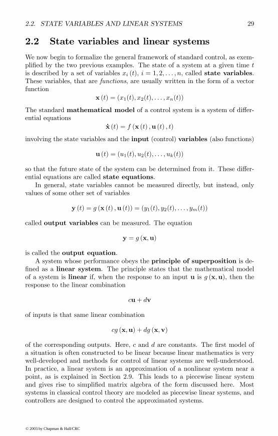
2.2. STATE VARIABLES AND LINEAR SYSTEMS 29

2.2 State variables and linear systems

We now begin to formalize the general framework of standard control, as exem-pliÞed by the two previous examples. The state of a system at a given time tis described by a set of variables xi (t), i = 1, 2, . . . , n, called state variables.These variables, that are functions, are usually written in the form of a vectorfunction

x (t) = (x1(t), x2(t), . . . , xn(t))

The standard mathematical model of a control system is a system of differ-ential equations

úx (t) = f (x (t) ,u (t) , t)

involving the state variables and the input (control) variables (also functions)

u (t) = (u1(t), u2(t), . . . , uk(t))

so that the future state of the system can be determined from it. These differ-ential equations are called state equations.In general, state variables cannot be measured directly, but instead, only

values of some other set of variables

y (t) = g (x (t) ,u (t)) = (y1(t), y2(t), . . . , ym(t))

called output variables can be measured. The equation

y = g (x,u)

is called the output equation.A system whose performance obeys the principle of superposition is de-

Þned as a linear system. The principle states that the mathematical modelof a system is linear if, when the response to an input u is g (x,u), then theresponse to the linear combination

cu+ dv

of inputs is that same linear combination

cg (x,u) + dg (x,v)

of the corresponding outputs. Here, c and d are constants. The Þrst model ofa situation is often constructed to be linear because linear mathematics is verywell-developed and methods for control of linear systems are well-understood.In practice, a linear system is an approximation of a nonlinear system near apoint, as is explained in Section 2.9. This leads to a piecewise linear systemand gives rise to simpliÞed matrix algebra of the form discussed here. Mostsystems in classical control theory are modeled as piecewise linear systems, andcontrollers are designed to control the approximated systems.



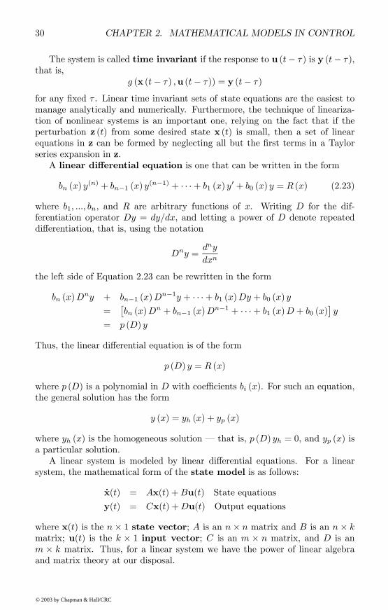
The system is called time invariant if the response to u (t− τ) is y (t− τ),that is,

g (x (t− τ) ,u (t− τ)) = y (t− τ)for any Þxed τ . Linear time invariant sets of state equations are the easiest tomanage analytically and numerically. Furthermore, the technique of lineariza-tion of nonlinear systems is an important one, relying on the fact that if theperturbation z (t) from some desired state x (t) is small, then a set of linearequations in z can be formed by neglecting all but the Þrst terms in a Taylorseries expansion in z.A linear differential equation is one that can be written in the form

bn (x) y(n) + bn−1 (x) y(n−1) + · · ·+ b1 (x) y0 + b0 (x) y = R (x) (2.23)

where b1, ..., bn, and R are arbitrary functions of x. Writing D for the dif-ferentiation operator Dy = dy/dx, and letting a power of D denote repeateddifferentiation, that is, using the notation

Dny =dny

dxn

the left side of Equation 2.23 can be rewritten in the form

bn (x)Dny + bn−1 (x)Dn−1y + · · ·+ b1 (x)Dy + b0 (x) y

=£bn (x)D

n + bn−1 (x)Dn−1 + · · ·+ b1 (x)D + b0 (x)¤y

= p (D) y

Thus, the linear differential equation is of the form

p (D) y = R (x)

where p (D) is a polynomial in D with coefficients bi (x). For such an equation,the general solution has the form

y (x) = yh (x) + yp (x)

where yh (x) is the homogeneous solution that is, p (D) yh = 0, and yp (x) isa particular solution.A linear system is modeled by linear differential equations. For a linear

system, the mathematical form of the state model is as follows:

úx(t) = Ax(t) +Bu(t) State equations

y(t) = Cx(t) +Du(t) Output equations

where x(t) is the n× 1 state vector; A is an n× n matrix and B is an n× kmatrix; u(t) is the k × 1 input vector; C is an m × n matrix, and D is anm × k matrix. Thus, for a linear system we have the power of linear algebraand matrix theory at our disposal.


2.2. STATE VARIABLES AND LINEAR SYSTEMS 31

Example 2.1 (Motion of an automobile) A classical example of a simpli-Þed control system is the motion of a car subject to acceleration and brakingcontrols. A simpliÞed mathematical model of such a system is

d2s

dt2+ a

ds

dt+ bs = f(t)

where s(t) represents position at time t, so that ds(t)dt represents velocity and

d2s(t)dt2 represents acceleration. The basic idea of the state variable approachis to select variables that represent the state of the system. Certainly, theposition s(t) and the velocity ds(t)

dt both represent states of the system. If welet x1(t) = s(t), then we are assigning a state variable x1(t) to represent theposition of the system. The velocity úx1(t) = ús(t) can be assigned another statevariable

x2(t) = úx1(t)

This is one of the state equations. Here, we have expressed one state in termsof the other. Proceeding further, note that x1(t) = úx2(t) = s(t) yields theacceleration term. From the second-order differential equation s(t) = −a ús(t)−bs(t) + f(t), we have

úx2(t) = −ax2(t)− bx1(t) + f(t)

This is the second of the state equations. For an nth order differential equationthere must be n Þrst-order state equations. In this case, for a second-orderdifferential equation, we have two Þrst-order differential equations. Castingthese two equations in vector-matrix form, we can write the set of state equationsas ·

úx1(t)úx2(t)

¸=

·0 1−b −a

¸ ·x1(t)x2(t)

¸+

·01

¸f (t)

that is of the form

úx(t) = Ax(t) +Bu(t)

where u (t) = f (t).To obtain both the position and the velocity of the system as outputs, we

can select y1(t) and y2(t) to represent the states x1(t) and x2(t), respectively.Placing these quantities in vector-matrix form, we obtain the output equation·

y1(t)y2(t)

¸=

·1 00 1

¸ ·x1(t)x2(t)

¸+

·00

¸f(t)

that is of the form

y(t) = Cx(t) +Du(t)

Note again that the outputs are expressed in terms of the system states.



2.3 Controllability and observabilityAn important Þrst step in solving control problems is to determine whether thedesired objective can be achieved by manipulating the chosen control variables.Intuitively, a control system should be designed so that the input can bringit from any state to any other state in a Þnite time, and also so that all thestates can be determined from measuring the output variables. The concepts ofcontrollability and observability formalize these ideas.A plant is controllable if at any given instant, it is possible to control each

state in the plant so that a desired outcome can be reached. In the case wherea mathematical model of the system is available in the form

úx (t) = F (x, u, t) (2.24)

the system úx (t) is said to be completely controllable if for any t0, any initialcondition x0 = x (t0), and any Þnal state xf , there exists a Þnite time T and acontrol function u (t) deÞned on the interval [t0, T ] such that x (T ) = xf . Notethat x (T ) is the solution of Equation 2.24 and clearly depends on the functionu (t). It can be shown that a linear, time-invariant system

úx (t) = Ax (t) +Bu (t) (2.25)

is completely controllable if and only if the n× nm controllability matrix

W =£B AB A2B · · · An−1B

¤(2.26)

has rank n, where A is n× n and B is n×m. More generally, the system

úx(t) = A(t)x(t) +B(t)u(t) (2.27)

y(t) = C(t)x(t)

with A a continuous n× n matrix, is completely controllable if and only if then× n symmetric controllability matrix

W (t0, t1) =

Z t1

t0

X (t)X−1 (t0)B (t)BT (t)¡X−1¢T (t0)XT (t) dt (2.28)

is nonsingular, where X (t) is the unique n× n matrix satisfyingdX (t)

dt= A (t)X (t) , X (0) = I (2.29)

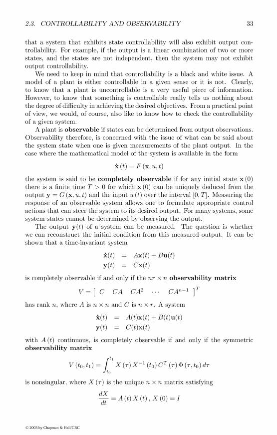
Other types of controllability can be deÞned. For example, output control-lability requires attainment of arbitrary Þnal output. The ability to control thestate gives rise to the notion that the output (response) of a system may also becontrollable, based on the assumption that if all the individual states in a sys-tem are controllable, and the output is a linear combination of the states, thenthe output must also be controllable. Generally, however, there is no guarantee


2.3. CONTROLLABILITY AND OBSERVABILITY 33

that a system that exhibits state controllability will also exhibit output con-trollability. For example, if the output is a linear combination of two or morestates, and the states are not independent, then the system may not exhibitoutput controllability.We need to keep in mind that controllability is a black and white issue. A

model of a plant is either controllable in a given sense or it is not. Clearly,to know that a plant is uncontrollable is a very useful piece of information.However, to know that something is controllable really tells us nothing aboutthe degree of difficulty in achieving the desired objectives. From a practical pointof view, we would, of course, also like to know how to check the controllabilityof a given system.A plant is observable if states can be determined from output observations.

Observability therefore, is concerned with the issue of what can be said aboutthe system state when one is given measurements of the plant output. In thecase where the mathematical model of the system is available in the form

úx (t) = F (x, u, t)

the system is said to be completely observable if for any initial state x (0)there is a Þnite time T > 0 for which x (0) can be uniquely deduced from theoutput y = G (x, u, t) and the input u (t) over the interval [0, T ]. Measuring theresponse of an observable system allows one to formulate appropriate controlactions that can steer the system to its desired output. For many systems, somesystem states cannot be determined by observing the output.The output y(t) of a system can be measured. The question is whether

we can reconstruct the initial condition from this measured output. It can beshown that a time-invariant system

úx(t) = Ax(t) +Bu(t)

y(t) = Cx(t)

is completely observable if and only if the nr × n observability matrixV =

£C CA CA2 · · · CAn−1

¤Thas rank n, where A is n× n and C is n× r. A system

úx(t) = A(t)x(t) +B(t)u(t)

y(t) = C(t)x(t)

with A (t) continuous, is completely observable if and only if the symmetricobservability matrix

V (t0, t1) =

Z t1

t0

X (τ)X−1 (t0)CT (τ)Φ (τ , t0) dτ

is nonsingular, where X (τ) is the unique n× n matrix satisfyingdX

dt= A (t)X (t) , X (0) = I



Once again the property of observability is also a black and white issue. Asystem either is or is not observable. A system that is observable can providethe necessary conditions of the plant variables as described above. However, theobserved plant variables may not be sufficient to reconstruct the entire plantdynamics.There is a duality result that connects these two concepts. Namely, a

linear system whose state model is of the form

úx(t) = A(t)x(t) +B(t)u(t)

y(t) = C(t)x(t)

where A, B, and C are matrices of appropriate sizes, is completely controllableif and only if the dual system

úx(t) = −AT (t)x(t) + CT (t)u(t)y(t) = BT (t)x(t)

is completely observable. This result is related to the fact that a matrix and itstranspose have the same rank.

2.4 StabilityStability analysis of a system to be controlled is the Þrst task in control design.In a general descriptive way, we can think of stability as the capacity of an objectto return to its original position, or to equilibrium, after having been displaced.There are two situations for stability: (1) the plant itself is stable (before theaddition of a controller), and (2) the closed-loop control system is stable. Allcontrolled systems must be designed to be stable regardless of the stability orinstability of the plant. Controllers must be able to handle disturbances thatare not characterized by the model of the system, such as a gust of wind actingon a car set to travel at a constant velocity, wind shear acting on a plane inßight, and so on. This is illustrated in Figure 2.10.The notion of stability can be viewed as a property of a system that is

continuously in motion about some equilibrium point. A point position a iscalled an equilibrium point of Equation 2.30 if f (a, t) = 0 for all t. Bychanging variables, y = x − a, the equilibrium point a can be transferred tothe origin. By this means, you can assume that a = 0. Thus, we will alwaysrefer to the stability at the point 0. The stability of a dynamical system that isdescribed by a differential equation of the form

úx =dx (t)

dt= f (x, t) (2.30)

is referred to as stability about an equilibrium point.When 0 is an equilibrium state of the system, the system will remain at 0

if started from there. In other words, if x (t0) = 0, then x (t) = 0 for all t ≥ t0.This is the intuitive idea of an equilibrium state.


2.4. STABILITY 35

Figure 2.10. Disturbance in system

In general, a dynamical system can have several equilibrium states. Also,the concept of stability about an equilibrium state can be formulated in manydifferent ways. Below is a popular concept of stability.

DeÞnition 2.1 The equilibrium state 0 of Equation 2.30 is said to be

1. stable (in the sense of Lyapunov) if for all ε > 0, there exists δ > 0 suchthat if kx (t0)k < δ then kx (t)k < ε for all t ≥ t0.

2. asymptotically stable if 0 is stable and limt→∞ x (t) = 0.

3. asymptotically stable in the large if 0 is asymptotically stable andlimt→∞ x (t) = 0 regardless of how large are the perturbations around 0.

In this deÞnition we use kx (t)k to denote the Euclidean norm, noting thatthe state space is some Rn. Of course 0 is unstable if there is an ε > 0 suchthat for all δ > 0 there exists x (t0) with kx (t0)k < δ and kx (t1)k > ε for somet1 ≥ t0.

Figure 2.11. Equilibrium points

The notions of stable and asymptotically stable refer to two different proper-ties of stability of 0. In other words, the nature of stability may vary from oneequilibrium point to another. The intuitive idea for stability is clear: for small



perturbations, from the equilibrium 0 at some time t0, the system remains closeto it in subsequent motion. This concept of stability is due to Lyapunov, andoften referred to as stability in the sense of Lyapunov.In Figure 2.11, the Þgure on the left represents stability in the sense of

Lyapunov if friction is ignored, and asymptotic stability if friction is taken intoaccount, whereas the Þgure in the center represents instability. The Þgure onthe right represents stability, which is a local condition. In the Þgure on theleft, even if friction is present, a ball would eventually return to equilibrium nomatter how large the disturbance. This is an illustration of asymptotic stabilityin the large.

2.4.1 Damping and system response

A control system produces an output, or response, for a given input, or stim-ulus. In a stable system, the initial response until the system reaches steadystate is called the transient response. After the transient response, the systemapproaches its steady-state response, which is its approximation for the com-manded or desired response. The nature and duration of the transient responseare determined by the damping characteristics of the plant.The possibility exists for a transient response that consists of damped oscilla-

tions that is, a sinusoidal response whose amplitude about the steady-statevalue diminishes with time. There are responses that are characterized as beingoverdamped (Figure 2.12 (a)) or critically damped (Figure 2.12 (b)). An

Figure 2.12. (a) Overdamped response (b) Critically damped response

overdamped system is characterized by no overshoot. This occurs when thereis a large amount of energy absorption in the system that inhibits the tran-sient response from overshooting and oscillating about the steady-state valuein response to the input. A critically damped response is characterized by noovershoot and a rise time that is faster than any possible overdamped responsewith the same natural frequency. Both are considered stable because there isa steady-state value for each type of response. Stated differently, the systemis in equilibrium. This equilibrium condition is achieved even if the systemis allowed to oscillate a bit before achieving steady state. Systems for which


2.4. STABILITY 37

Figure 2.13. (a) Underdamped response (b) Undamped response

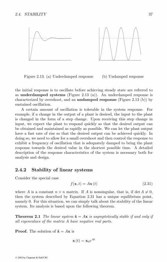
the initial response is to oscillate before achieving steady state are referred toas underdamped systems (Figure 2.13 (a)). An underdamped response ischaracterized by overshoot, and an undamped response (Figure 2.13 (b)) bysustained oscillation.A certain amount of oscillation is tolerable in the system response. For

example, if a change in the output of a plant is desired, the input to the plantis changed in the form of a step change. Upon receiving this step change ininput, we expect the plant to respond quickly so that the desired output canbe obtained and maintained as rapidly as possible. We can let the plant outputhave a fast rate of rise so that the desired output can be achieved quickly. Indoing so, we need to allow for a small overshoot and then control the response toexhibit a frequency of oscillation that is adequately damped to bring the plantresponse towards the desired value in the shortest possible time. A detaileddescription of the response characteristics of the system is necessary both foranalysis and design.

2.4.2 Stability of linear systems

Consider the special casef(x, t) = Ax (t) (2.31)

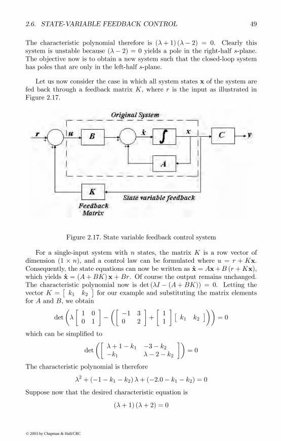
where A is a constant n × n matrix. If A is nonsingular, that is, if detA 6= 0,then the system described by Equation 2.31 has a unique equilibrium point,namely 0. For this situation, we can simply talk about the stability of the linearsystem. Its analysis is based upon the following theorem.

Theorem 2.1 The linear system úx = Ax is asymptotically stable if and only ifall eigenvalues of the matrix A have negative real parts.

Proof. The solution of úx = Ax is

x (t) = x0eAt



where

eAt =∞Xk=0

tk

k!Ak

with A0 the identity n× n matrix and x0 = x (0). Now

eAt =mXk=1

hBn1 +Bn2t+ · · ·+Bnαk tαk−1

ieλkt (2.32)

where the λks are eigenvalues of A, the αks are coefficients of the minimumpolynomial of A, and the Bns are constant matrices determined solely by A.Thus, °°eAt°° ≤

mXk=1

αkXi=1

ti−1°°eλkt°° kBnik

=mXk=1

αkXi=1

ti−1eRe(λk)t kBnik

where Re(λk) denotes the real part of λk.Thus, if Re(λk) < 0 for all k, then

limt→∞ kx (t)k ≤ lim

t→∞ kx0k°°eAt°° = 0

so that the origin is asymptotically stable.Conversely, suppose the origin is asymptotically stable. Then Re(λk) < 0

for all k, for if there exists some λk such that Re(λk) > 0, then we see fromEquation 2.32 that limt→∞ kx (t)k =∞ so that the origin is unstable.Such a matrix, or its characteristic polynomial, is said to be stable.

Example 2.2 The solution of a second-order constant-coefficient differentialequation of the form

d2y

dt2+ a

dy

dt+ by = 0

is stable if the real parts of the roots

s1 = −12

³a−

pa2 − 4b

´s2 = −1

2

³a+

pa2 − 4b

´of the characteristic polynomial s2+as+b lie in the left-half s-plane. In practice,the characteristic polynomial is often found by taking the Laplace transform toget the transfer function

L (y) = y0 (0) + (a+ s) y (0)s2 + as+ b

The roots of s2 + as+ b are called the poles of the rational function L (y).If bounded inputs provide bounded outputs, this is called BIBO stability. If

a linear system is asymptotically stable, then the associated controlled systemis BIBO stable.


2.4. STABILITY 39

2.4.3 Stability of nonlinear systems

Stability analysis for nonlinear systems is more complicated than for linear sys-tems. There is, nevertheless, an extensive theory for control of nonlinear sys-tems, based on Lyapunov functions. This theory depends on the mathematicalmodels of the systems, and when considering fuzzy and neural control as analternative to standard control of nonlinear systems, we will need to considerother approaches to stability analysis.For a nonlinear system of the form

úx = f (x) , f (0) = 0 (2.33)

with x (t0) = x0, it is possible to determine the nature of stability of the originwithout solving the equation to obtain x (t). Sufficient conditions for stabilityof an equilibrium state are given in terms of the Lyapunov function. Theseconditions generalize the well-known property that an equilibrium point is stableif the energy is a minimum.

DeÞnition 2.2 A Lyapunov function for a system úx = f (x) is a functionV : Rn → R such that

1. V and all its partial derivatives ∂V∂xi, i = 1, 2, . . . , n are continuous.

2. V (0) = 0 and V (x) > 0 for all x 6= 0 in some neighborhood kxk < k of0. That is, V is positive deÞnite.

3. For x (t) = (x1 (t) , . . . , xn (t)) satisfying úx = f (x) with f (0) = 0,

úV (x) =∂V

∂x1úx1 + · · ·+ ∂V

∂xnúxn

is such that úV (0) = 0 and úV (x) ≤ 0 for all x in some neighborhood of 0.In other words, úV is negative semideÞnite.

Theorem 2.2 For a nonlinear system of the form

úx = f (x) , f (0) = 0

the origin is stable if there is a Lyapunov function V for the system úx = f (x),f (0) = 0.

Proof. Take a number k > 0 satisfying both V (x) > 0 and úV (x) ≤ 0 for allx 6= 0 in the neighborhood kxk < k of 0. Then there exists a continuous scalarfunction ϕ : R → R with ϕ (0) = 0 that is strictly increasing on the interval[0, k] such that

ϕ (kxk) ≤ V (x)for all x in the neighborhood kxk < k of 0. Given ε > 0, then since ϕ (ε) > 0,V (0) = 0 and V (x) is continuous, and x0 = x (t0) can be chosen sufficientlyclose to the origin so that the inequalities

kx0k < ε, V (x0) < ϕ (ε)



are simultaneously satisÞed. Also, since úV (x) ≤ 0 for all x in the neighborhoodkxk < k of 0, t0 ≤ t1 ≤ k implies

V (x (t1)) ≤ V (x (t0)) < ϕ (ε)Thus, for all x in the neighborhood kxk < k of 0, t0 ≤ t1 ≤ k implies

kx (t1)k < εsince we know that ϕ (kx (t1)k) ≤ V (x (t1)) < ϕ (ε), and kx (t1)k ≥ ε wouldimply ϕ (kx (t1)k) ≥ ϕ (ε) by the property that ϕ is strictly increasing on [0, k].Taking δ = ε, we see by DeÞnition 2.1 that the origin is stable.

The proof of the following theorem is similar. A function úV : Rn → R is saidto be negative deÞnite if úV (0) = 0 and for all x 6= 0 in some neighborhoodkxk < k of 0, úV (x) < 0.Theorem 2.3 For a nonlinear system of the form

úx = f (x) , f (0) = 0 (2.34)

the origin is asymptotically stable if there is a Lyapunov function V for thesystem, with úV negative deÞnite.

Here is an example.

Example 2.3 Consider the nonlinear system

úx = f (x)

where

x =

µx1x2

¶, úx =

µúx1úx2

¶= f (x) =

µf1 (x)f2 (x)

¶with

f1 (x) = x1¡x21 + x

22 − 1

¢− x2f2 (x) = x1 + x2

¡x21 + x

22 − 1

¢The origin (0, 0) is an equilibrium position. The positive deÞnite function

V (x) = x21 + x22

has its derivative along any system trajectory

úV (x) =∂V

∂x1úx1 +

∂V

∂x2úx2

= 2x1£x1¡x21 + x

22 − 1

¢− x2¤+ 2x2 £x1 + x2 ¡x21 + x22 − 1¢¤= 2

¡x21 + x

22 − 1

¢ ¡x21 + x

22

¢When x21 + x

22 < 0, we have úV (x) < 0, so that (0, 0) is asymptotically stable.


2.4. STABILITY 41

2.4.4 Robust stability

The problem of robust stability in control of linear systems is to ensure systemstability in the presence of parameter variations. We know that the origin isasymptotically stable if all the eigenvalues of the matrix A have negative realparts. When A is an n × n matrix, there are n eigenvalues that are roots ofthe associated characteristic polynomial Pn(x) =

Pnk=0 akx

k. Thus, when thecoefficients ak are known (given in terms of operating parameters of the plant),it is possible to check stability since there are only Þnitely many roots to check.These parameters might change over time due to various factors such as

wearing out or aging; and hence, the coefficients ak should be put in toleranceintervals [a−k , a

+k ], allowing each of them to vary within the interval. Thus, we

have an inÞnite family of polynomials Pn, indexed by coefficients in the intervals[a−k , a

+k ], k = 0, 1, 2, ..., n. In other words, we have an interval-coefficient

polynomialnXk=0

[a−k , a+k ]x

k

This is a realistic situation where one needs to design controllers to handlestability under this type of uncertainty that is, regardless of how the coef-Þcients ak are chosen in each [a

−k , a

+k ]. The controller needs to be robust in the

sense that it will keep the plant stable when the plant parameters vary withinsome bounds. For that, we need to be able to check the n roots of membersof an inÞnite family of polynomials. It seems like an impossible task. But ifthat were so, there would be no way to construct controllers to obtain robuststability.Mathematically, it looks as though we are facing an inÞnite problem. How-

ever, like some other problems that appear to be inÞnite problems, this is a Þniteproblem. This discovery, due to Kharitonov in 1978, makes robust control pos-sible for engineers to design. Here is an outline of his result.

Theorem 2.4 (Kharitonov) Suppose [a−k , a+k ], k = 0, 1, ..., n is a family of

intervals. All polynomials of the form Pn(x) =Pn

k=0 akxk, where ak ∈ [a−k , a+k ],

are stable if and only if the following four Kharitonov canonical polynomials arestable:

K1(x) = a−0 + a−1 x+ a

+2 x

2 + a+3 x3 + a−4 x

4 + a−5 x5 + a+6 x

6 + · · ·K2(x) = a+0 + a

+1 x+ a

−2 x

2 + a−3 x3 + a+4 x

4 + a+5 x5 + a−6 x

6 + · · ·K3(x) = a+0 + a

−1 x+ a

−2 x

2 + a+3 x3 + a+4 x

4 + a−5 x5 + a−6 x

6 + · · ·K4(x) = a−0 + a

+1 x+ a

+2 x

2 + a−3 x3 + a−4 x

4 + a+5 x5 + a+6 x

6 + · · ·Note that the pattern for producing these four polynomials is obtained by

repetitions of the symbol pattern− − + ++ + − −+ − − +− + + −



by the superscripts of the lower and upper bounds of the intervals.

Example 2.4 Take polynomials P2 (x) = a0+ a1x+ a2x2 where a0 ∈ [0.9, 1.1],a1 ∈ [−0.9, 0.1], and a2 ∈ [0.9, 1.1]. The four Kharitonov canonical polynomialsare

K1(x) = 0.9− 0.9x+ 1.1x2K2(x) = 1.1 + 0.1x+ 0.9x2

K3(x) = 1.1− 0.9x+ 0.9x2K4(x) = 0.9 + 0.1x+ 1.1x2

Two of these polynomials, K1(x) and K3(x), have roots with positive real parts,0.409 and 0.5, so the interval-coefficient polynomial with these intervals does notrepresent a stable system. On the other hand, if a0 ∈ [1.0, 1.1], a1 ∈ [0.9, 1.0],and a2 ∈ [0.9, 1.0], the four Kharitonov canonical polynomials are

K1(x) = 1 + 0.99x+ x2

K2(x) = 1.1 + x+ 0.99x2

K3(x) = 1.1 + 0.99x+ 0.99x2

K4(x) = 1 + x+ x2

all of whose roots have negative real parts, and we know that a system producingthese polynomials is stable.

2.5 Controller designThere is a two-fold objective in the design of controllers. First, the overallcontrol loop must be stable. Second, the input to the plant must be such thatthe desired set-point is achieved in minimum time within some speciÞed criteria.Both of these objectives require full knowledge of the plant.1

The fundamental objective in feedback control is to make the output of aplant track the desired input. Generally, this is referred to as set-point control.The controller can be placed either in the forward path (in series) with the plantor in the feedback path. Figures 2.14 (a) and (b) illustrate such conÞgurations.Most of the conventional design methods in control systems rely on the so-

called Þxed-conÞguration design in that the designer at the outset decidesthe basic conÞguration of the overall designed system and the location wherethe controller is to be positioned relative to the controlled process. The prob-lem then involves the design of the elements of the controller. Because mostcontrol efforts involve the modiÞcation or compensation of the system perfor-mance characteristics, the general design using Þxed conÞguration is also calledcompensation.

1We are restricting our discussion of classical methods to only those that have a directbearing on the fuzzy controllers which will be discussed later. The reader should be awarethat classical methods exist for many other types of controller designs that are very powerfuland have been used extensively in modern control systems.


2.5. CONTROLLER DESIGN 43

Figure 2.14. Set-point control

The most commonly used conÞguration is shown in Figure 2.14 (a) in whichthe controller is placed in series with the plant to be controlled. This typeof control is referred to as series or cascade compensation. The PID con-troller has a conÞguration illustrated in Figure 2.14 (a). In Figure 2.14 (b) thecompensator is placed in the minor feedback path and is usually referred toas feedback compensation. State-variable and output-feedback controllers havethe conÞguration shown in Figure 2.14 (b).Standard control is based on knowledge of a mathematical model of the

system. The mathematical model can take on basically two forms:

1. The actual model of the system.

2. An estimated model of the system.

For the classical design of controllers, we need to know something numericalabout the system. The so-called numerical approach requires that we knowsomething about the dynamics of the system. As brießy discussed earlier, themodel of the plant can be described by a set of equations. Typically, what wehave is a set of nonlinear differential equations for which a transfer functiondoes not exist. Designing a controller for a nonlinear system requires thatthe system Þrst be linearized about some nominal operating point. From thislinearized model, a transfer function of the plant, that is, the ratio of theoutput function to the input function, can be derived.These computations are normally done in the frequency domain obtained

by taking Laplace transforms of the state equations. The Laplace transformof a function x (t) is deÞned as

x (s) =

Z ∞

0

x (t) e−stdt



for values of s for which this improper integral converges. Taking Laplace trans-forms of the system of equations

úx (t) = Ax (t) +Bu (t) (2.35)

y (t) = Cx (t) +Eu (t)

with x (0) = 0, we obtain

sx (s) = Ax (s) +Bu (s) (2.36)

y (s) = Cx (s) + Eu (s)

Writing sx (s) = sIx (s) where I is the identity matrix of the appropriate size,we get

(sI −A) x (s) = Bu (s) (2.37)

and inverting the matrix sI −A,

y (s) = C (sI −A)−1Bu (s) +Eu (s) (2.38)

=³C (sI −A)−1B +E

´u (s)

Thus, the system transfer function

G (s) = C (sI −A)−1B +E (2.39)

satisÞesG (s) u (s) = y (s) (2.40)

and thus describes the ratio between the output y (s) and the input u (s). The

ratioC(s)

R(s)=y (s)

u (s)is also known as the closed-loop control ratio.

There are a number of other reasons why transfer functions obtained from theLaplace transform are useful. A system represented by a differential equation isdifficult to model as a block diagram, but the Laplace transform of the systemhas a very convenient representation of this form. Another reason is that inthe solution x (t) = eAtx (0) +

R t0eA(t−τ)Bu (τ) dτ to the differential equation

model in Equation 2.35, the input u appears inside the convolution integral,whereas in the transfer model, x (s) becomes a rational function multiplied bythe input u. Also, the transfer function in the frequency domain is analytic,except at a Þnite number of poles, and analytic function theory is very usefulin analyzing control systems.In the closed-loop feedback system shown in Figure 2.15, R (s) = u (s) is the

reference input, C(s) = y (s) is the system output, G (s) is the closed-loopcontrol ratio, E (s) is the error, and H (s) is the feedback transfer function.From this Þgure we can derive the following relationships:

1. The output of the plant is C(s) = G(s)E(s).



Figure 2.15. Closed-loop feedback system

2. The error between the input value E(s) and the output C(s) of the systemampliÞed or reduced by the feedback transfer function H(s) is

E(s) = R(s)−H(s)C(s)

3. Substituting the error E(s) into the equation for output of the plant, weget

C(s) = G(s)[R(s)−H(s)C(s)]

4. Collecting terms and rearranging, we get

C(s)

R(s)=

G(s)

1 +G(s)H(s)

that we can write asG(s)

1 +G(s)H(s)=N(s)

D(s)

where N(s) and D(s) are polynomials in the variable s.

Factoring N(s) displays all the zeros of the plant transfer function; factoringD(s) displays all the poles of the plant transfer function. The roots of D(s) arecalled the characteristic roots of the system; D(s) = 0 is the characteristicequation.A knowledge of the poles and zeros of the plant transfer function provides

the means to examine the transient behavior of the system, and to obtain limitson the loop gain to guarantee stability of the system. If a system is inherentlyunstable, such as the case of an inverted pendulum, the plant transfer functionprovides the designer with information on how to compensate the pole-zerobehavior of the plant with that of a controller. In this case, the controller polesand zeros are selected in combination with the plant poles and zeros to producea transient response that meets the necessary design requirements.Knowledge of the plant mathematical model clearly provides the means to

obtain the mathematical form of the controller. We can choose to place the



Figure 2.16. Controller in forward or feedback path

controller either in the forward path or in the feedback path as illustrated inFigure 2.16. Once the structure of the control system is decided upon, suitableparameters can then be chosen for the controller model to obtain the desiredplant response characteristics.Consider for example, the closed-loop transfer function of an unstable plant

given by the control ratio

Gp(s) =C(s)

R(s)=

1

(s+ 1)(s− 2)where C(s) is the plant output and R(s) is the plant input. Upon examining theroots, it is clear that the system is indeed unstable that is, the root satisfyings− 2 = 0 lies in the right-half s-plane. Suppose we wish to develop a controllersuch that the system becomes stable and has speciÞc response characteristics.Let Gc(s) and Gp(s) represent the controller and plant transfer functions, re-spectively. If the controller is in the forward path, then the closed-loop transferfunction would be given as

G1(s) =Gc(s)Gp(s)

1 +Gc(s)Gp(s)

Substituting the given plant transfer function and rearranging yields

G1(s) =Gc(s)

(s+ 1)(s− 2) +Gc(s)The denominator of this new control ratio represents the characteristic equationof the system that includes both the controller and the plant. We are now in a



position to choose any desired set of roots that yield satisfactory performance.Suppose we choose the desired characteristic equation as

(s+ 2)(s+ 3) = 0

Equating the denominator of G1(s) with the desired characteristic equationyields

(s+ 1)(s− 2) +Gc(s) = (s+ 2)(s+ 3)Expanding and simplifying yields the controller mathematical form

Gc(s) = (6s+ 8)

Suppose we choose the feedback path for the controller design. In this casethe resulting closed-loop transfer function would be given as

G2(s) =Gp(s)

1 +Gp(s)Gc(s)

Substituting the given plant transfer function and rearranging yields

G2(s) =1

(s+ 1)(s− 2) +Gc(s)Once again, if we choose the desired characteristic equation as (s+2)(s+3) = 0,we obtain the same result as before, namely,

Gc(s) = (6s+ 8)

In either case, the controller is of the form

Gc(s) = KDs+KP

This clearly has meaning in terms of derivative and proportional gain control.More will be discussed along these lines in later sections. The point we wish tomake here is that given the mathematical model of a plant, it is entirely possibleto obtain a suitable controller design. What we have seen in this example isthe addition of terms to the overall closed-loop transfer function such that somedesired performance criteria can be met. In the Þrst case where the controlleris placed in the forward path, the resulting closed-loop transfer function of thecontrol system is

G1(s) =6s+ 8

s2 + 5s+ 6

where the numerator term 6s + 8 represents the addition of a zero to thetransfer function. Such manipulations of the plant mathematical models toyield desired plant responses is characterized in classical control techniques asroot locus analysis and the criterion used to adjust the open-loop sensitivitygain is called the Routh-Hurwitz stability criterion. Adjusting the open-loop sensitivity gain, and placing limits on the range of this gain will assurestable operation of the system within prescribed limits. We urge the readerto refer to one of many excellent control systems books in the literature for acomplete treatise on this topic. See [16] for example.



2.6 State-variable feedback controlHere we address a controller design technique known as state-variable feedbackcontrol. The concept behind state-variable feedback control is to determine thepoles of the transfer function of the closed-loop system and make changes so thatnew poles are assigned that meet some design criteria. We will see that the basicsolution is to place poles in the controller such that the root loci of the overallsystem is moved into the left-half s-plane. As mentioned earlier, the objective incontrol systems design is to stabilize an otherwise unstable plant. The methodby which an inherently unstable system can be made stable by reassigning itspoles to lie in the left-half s-plane is referred to as pole placement. The theorybehind this technique comes from the result in Theorem 2.1 on page 37 thatstates that the linear system úx = Ax is asymptotically stable if and only if alleigenvalues of the matrix A have negative real parts, and the fact that theseeigenvalues are the poles of the transfer function.It is not necessary that only unstable systems be considered for such con-

trol. Even stable systems that do not meet the criteria for a suitable transientresponse can be candidates for state-variable feedback control. However, it isnecessary that all states of the original system be accessible and that the systembe completely controllable.

2.6.1 Second-order systems

We can discuss state-variable feedback control with some simple examples.These examples are chosen only to demonstrate how the behavior of a systemcan be modiÞed and are not intended to provide a complete theoretical eval-uation of state-variable feedback control. There are excellent references thatprovide full details of this type of control, such as [16] and [28], and the readeris strongly urged to refer to the literature on this topic.

Example 2.5 Consider a second-order system represented by the state andoutput equations as follows:·

úx1úx2

¸=

· −1 30 2

¸ ·x1x2

¸+

·11

¸u

y =£1 0

¤ · x1x2

¸These equations are of the form úx = Ax+Bu, the state equation, and y = Cx,the output equation. The eigenvalues of this system can be determined byconsidering det [λI −A] = 0, the characteristic polynomial of the system. Thisgives

det

µλ

·1 00 1

¸−· −1 30 2

¸¶= 0

that simpliÞes to

det

µ·λ+ 1 −30 λ− 2

¸¶= (λ+ 1) (λ− 2) = 0


2.6. STATE-VARIABLE FEEDBACK CONTROL 49

The characteristic polynomial therefore is (λ+ 1) (λ− 2) = 0. Clearly thissystem is unstable because (λ− 2) = 0 yields a pole in the right-half s-plane.The objective now is to obtain a new system such that the closed-loop systemhas poles that are only in the left-half s-plane.

Let us now consider the case in which all system states x of the system arefed back through a feedback matrix K, where r is the input as illustrated inFigure 2.17.

Figure 2.17. State variable feedback control system

For a single-input system with n states, the matrix K is a row vector ofdimension (1 × n), and a control law can be formulated where u = r + Kx.Consequently, the state equations can now be written as úx = Ax+B (r +Kx),which yields úx = (A+BK)x+ Br. Of course the output remains unchanged.The characteristic polynomial now is det (λI − (A+BK)) = 0. Letting thevector K =

£k1 k2

¤for our example and substituting the matrix elements

for A and B, we obtain

det

µλ

·1 00 1

¸−µ· −1 3

0 2

¸+

·11

¸ £k1 k2

¤¶¶= 0

which can be simpliÞed to

det

µ·λ+ 1− k1 −3− k2−k1 λ− 2− k2

¸¶= 0

The characteristic polynomial is therefore

λ2 + (−1− k1 − k2)λ+ (−2.0− k1 − k2) = 0Suppose now that the desired characteristic equation is

(λ+ 1) (λ+ 2) = 0



orλ2 + 3λ+ 2 = 0

Comparing the coefficients, we get (−1− k1 − k2) = 3 and (−2.0−k1−k2) = 2,which yields two identical equations (k1 + k2) = −4. While this results in anonunique solution for the feedback gains k1 and k2, we see that any set ofparameters satisfying (k1 + k2) = −4 will shift the pole originally located in theright-half s-plane, namely (λ− 2) = 0, to the left-half s-plane at (λ+ 2) = 0.

2.6.2 Higher-order systems

Implementing state-variable feedback control for higher-order systems is sim-pliÞed by Þrst converting the given system to a controller canonical form inwhich the elements of the characteristic matrix have a prescribed structure. Forexample, given the characteristic equation of a system as

Q(λ) = λn + αn−1λn−1 + · · ·+ α1λ+ α0the controller canonical form of the characteristic matrix is

Ac =

0 1 00 0 1 0

0 0. . . 1 0

0 1−α0 −α1 · · · −αn−2 −αn−1

The entries in the last row of the Ac matrix are the negatives of the coefficientsof the characteristic polynomial. In addition, the input conditioning matrix Bcfor the controller canonical realization is of the form

Bc = [0 0 · · · 0 1]T

Now, if we choose the feedback matrix

K = [k1 k2 · · · kn−1 kn]

the resulting matrix obtained from [A+BK] can be written as:

Acf =

0 10 1

0. . . 1

0 1−α0 + k1 −α1 + k2 · · · −αn−2 + kn−1 −αn−1 + kn

Comparing the coefficients of the given system with the desired system yields

the feedback gains. Therefore, the canonical form of system representation ismore convenient for determining the feedback gains when dealing with higher-order systems.


2.6. STATE-VARIABLE FEEDBACK CONTROL 51

Example 2.6 Consider an unstable third-order system given by the set of stateand output equations as úx1

úx2úx3

=

1 6 −3−1 −1 1−2 2 0

x1x2x3

+ 111

uy =

£0 0 1

¤ x1x2x3

We notice that the system is not in canonical form and proceed to develop thecontroller canonical realization. To do this, we Þrst obtain the transfer functionof the given system as

Y (s)

U(s)= C [sI −A]−1B +D

This can be done very easily using Matlab by specifying the A, B, C, and Dmatrices and using theMatlab function ss2tf to obtain the transfer functionof the system. The following Matlab code illustrates this process:

a=[1 6 -3;-1 -1 1;-2 2 0]; %Specify the A matrixb=[1;1;1]; %Specify the B matrixc=[0 0 1]; %Specify the C matrixd=0; %Specify the D matrix[num,den]=ss2tf(a,b,c,d,1); %Note: the 1 indicates a single-input system

The resulting transfer function is

Y (s)

U(s)=

s2 − 13s3 − 3s+ 2

The denominator of the transfer function factors as (s+ 2) (s− 1)2, display-ing the roots of the characteristic equation and clearly indicating an unstablesystem. From the method discussed above, the characteristic matrix for thecontroller canonical realization may be obtained directly as

Ac =

0 1 00 0 1

−2 3 0

Suppose the desired set of eigenvalues for the system is

λ1, λ2 = −1± j, λ3 = −4

which gives the characteristic polynomial

Q(λ) = λ3 + 6λ2 + 10λ+ 8



From this, we can determine the desired characteristic matrix as

Acf =

0 1 00 0 1

−8 −10 −6

Comparing the last row of coefficients between Ac and Acf , we obtain the feed-back gain matrix

K = [−6 − 13 − 6]

For the examples considered here, we see a fairly straightforward approachto implementing state-variable feedback control. However, as mentioned previ-ously, all states of the original system must be accessible, and the system mustbe completely controllable. Therefore, we need to know a priori that the sys-tem is fully controllable before attempting to implement state-variable feedbackcontrol.Such a priori knowledge can be obtained by investigating the rank of the

n× nm controllability matrix£B AB A2B · · · An−1B

¤formed by the A and B matrices of the original system (see page 32). Recallthat an nth-order single-input system is fully controllable if and only if

Rank£B AB A2B · · · An−1B

¤= n

This says that if the rank of the controllability matrix is less than n, thesystem is not fully controllable. A system being not fully controllable impliesthat one or more states of the system are not directly controllable. This is dueto pole-zero cancellations in the system transfer function as the next exampleindicates.

Example 2.7 Consider the state and output equations of a second-order sys-tem given by ·

úx1úx2

¸=

· −2 0−1 −1

¸ ·x1x2

¸+

·11

¸u

y =£0 1

¤ · x1x2

¸Computing the transfer function G(s) = C [sI −A]−1B +D yields

G(s) =(s+ 1)

(s+ 1)(s+ 2)

in which the pole and zero located at s = −1 cancel, making the system uncon-trollable at the eigenvalue λ = −1. Whether or not the system is fully control-lable can also be veriÞed by computing the rank of the controllability matrix asfollows:

Rank

·11

· −2 0−1 −1

¸ ·11

¸ ¸= Rank

·1 −21 −2

¸= 1


2.7. PROPORTIONAL-INTEGRAL-DERIVATIVE CONTROL 53

This computation showing Rank < 2 implies the system is not fully controllable,but this does not, by itself, indicate which of the two eigenvalues is uncontrol-lable.

2.7 Proportional-integral-derivative control

Most industrial systems are controlled by classical proportional-integral-deriva-tive (PID) controllers (including P, PD, and PI). This is done despite the systembeing nonlinear and despite the fact that the simplicity of the concept oftenlimits the performance. The reason why PID controllers have gained such pop-ularity is that detailed knowledge about the system is not required, but thecontroller can be tuned by means of simple rules of thumb or by PID auto-tuners.In this section, we demonstrate with several examples the design of con-

trollers using the standard approach. These same examples will be developedusing a fuzzy, neural, or neural-fuzzy approach in later chapters. The automo-bile cruise control and temperature control problems are examples of regulationproblems, where the fundamental desired behavior is to keep the output of thesystem at a constant level, regardless of disturbances acting on the system.The servomotor dynamics control problem is a component of a servo problem,where the fundamental desired behavior is to make the output follow a referencetrajectory.

2.7.1 Example: automobile cruise control system

In this example, we develop a simple model of an automobile cruise controlsystem. The control objective is to maintain a speed preset by the driver. If we

Figure 2.18. Mass and damper system

neglect the inertia of the wheels, and assume that friction (which is proportionalto the cars speed) is what is opposing the motion of the car, then the plantdescription is reduced to the simple mass and damper system shown in Figure



2.18. Using Newtons law of motion, the model equations for this system are

mdv

dt+ bv = f

y = v

where f is the force produced by the engine and v is the measured velocity of theautomobile. For this example, Let us assume that m = 1000 kg, b = 50 Newtonseconds/meter, and f = 500 Newtons, a constant force produced by the engine.When the engine produces a 500 Newton force, the car will reach a maximumvelocity of 10 meters/second. An automobile should be able to accelerate up tothat speed in less than 5 seconds. For this simple cruise control system, we canassume an allowable overshoot of 10% on the velocity and a 2% steady-stateerror.The next step is to Þnd the transfer function of the system above. For this,

we need to take the Laplace transform of the model equations. When Þnding thetransfer function, zero initial conditions must be assumed. Performing Laplacetransforms of the two equations gives

msV (s) + bV (s) = F (s)

Y (s) = V (s)

Since our output is the velocity, Let us express V (s) in terms of Y (s) and obtain

msY (s) + bY (s) = F (s)

The plant transfer function therefore becomes

Y (s)

F (s)=

1

ms+ b

Substituting m = 1000 kg, b = 50 Newton seconds/meter assumed for the auto-mobile, the transfer function is

Y (s)

F (s)=

1

1000s+ 50=(1/1000)

s+ 0.05

For a constant force of 500 Newtons produced from the start, with the automo-bile initially at rest, this represents a step input where

F (s) =500

s

We can now compute the open-loop response of the system to examine how wellthe system behaves without any controller action.The open-loop response of the plant is that produced by the engine force

acting on the mass of the automobile. In this analysis, there is no controlleraction as there is no feedback. Therefore, the output response is

Y (s) =(1/1000)

s+ 0.05F (s) =

·(1/1000)

s+ 0.05

¸ ·500

s

¸=

0.5

s (s+ 0.05)



Performing partial fractions expansion, we obtain

Y (s) =10

s− 10

s+ 0.05

The inverse Laplace transform yields

y(t) = 10u(t)− 10e−0.05tu(t)where u(t) is a unit step. The graph in Figure 2.19 shows that the vehicle takesmore than 100 seconds to reach the steady-state speed of 10 meters/second.Clearly, this does not satisfy our rise time criterion of less than 5 seconds.

0

2

4

6

8

10

20 40 60 80 100t

Figure 2.19. y(t) = 10u(t)− 10e−0.05tu(t)

From the above analysis, we have determined that a controller is needed toimprove the performance. The performance of this system can be improved byproviding a unity feedback controller. Figure 2.20 is the block diagram of atypical unity feedback system.

Figure 2.20. Unity feedback system

We choose the standard PID transfer function for the controller, namely,

Gc(s) = KP +KIs+KDs =

KDs2 +KP s+KI

s

The plant transfer function is as derived above, namely,

Gp(s) =1

ms+ b



The objective in the controller design then is to select the appropriate parame-ters for KP , KI , and KD to satisfy all design criteria.To design a PID controller for a given system, follow the steps shown below

to obtain a desired response.

1. Obtain the open-loop response and determine what needs to be improved.

2. Add proportional control to improve the rise time KP > 0.

3. Add derivative control to improve the overshoot KD > 0.

4. Add integral control to eliminate the steady-state error KI > 0.

5. Adjust each of KP , KI , and KD until a desired overall response is ob-tained.

Working through each of the steps listed above, we have already seen thatthe open-loop response is not satisfactory in that the rise time is inadequate forthe automobile to reach a velocity of 10 meters/second in less than 5 seconds.We must therefore provide some proportional gain, KP > 0, such that the risetime is smaller that is, the velocity reaches 10 meters/second in less than5 seconds. In general, it is intuitive to think that if the rise time is made toosmall, the velocity might reach the desired value at the expense of creatinga large overshoot before settling down to the desired value. Naturally then,we need to be concerned about how we can best control the overshoot as aconsequence of reducing the rise time.To achieve only proportional control action, we select KP > 0 and set KD =

KI = 0 in the controller transfer function Gc(s). Selecting values for any of theconstants is on a purely trial and error basis. However, we should keep in mindthat the proportional gain KP affects the time constant and consequently therate of rise.From the control system diagram, we see that the controller and plant can

be combined into a single transfer function, namely,

G(s) = Gc(s)Gp(s) = KP

µ1

ms+ b

¶The closed-loop transfer function therefore is determined as

Y (s)

F (s)=

G(s)

1 +G(s)H(s)

where H(s) is the feedback transfer function. In this case, since we have chosena unity feedback system, we set H(s) = 1. We therefore obtain the closed-looptransfer function of the system as

Y (s)

F (s)=

G(s)

1 +G(s)=

KP

ms+b

1 + KP

ms+b

=KP

ms+ b+KP



Let us select KP = 100 as a start and see what happens. Substituting valuesfor KP , m, and b we get the closed-loop transfer function as

Y (s)

F (s)=

100

1000s+ 50 + 100=

100

1000s+ 150=

0.1

s+ 0.15

Since we are interested in obtaining a desired velocity of 10 meters/second,we need to provide a step input of amplitude 10 meters/second. Therefore,using F (s) = 10/s, we obtain the closed-loop response Y (s) as,

Y (s) =0.1

s+ 0.15F (s) =

µ0.1

s+ 0.15

¶µ10

s

¶=

1

s (s+ 0.15)=

10.15

s−

10.15

s+ 0.15

=6. 6667

s− 6. 6667

s+ 0.15

The time-domain solution for this is y(t) = 6. 6667u(t) − 6. 6667e−0.15tu(t),shown in Figure 2.21.

0

2

4

6

8

10

20 40 60 80 100t

Figure 2.21. Time-domain solution

Once again, we see that choosing KP = 100 still does not satisfy our risetime criterion of less than 5 seconds. However, we do see an improvement overthe open-loop response shown earlier. Choosing KP = 1000, and carrying outan analysis similar to the above shows that the closed-loop response satisÞes theperformance criteria for rise time.

Y (s)

F (s)=

1000

1000s+ [50 + 1000]=

1000

1000s+ 1050=

1

s+ 1.05

Y (s) =1

s+ 1.05F (s) =

·1

s+ 1.05

¸ ·10

s

¸=

10

s (s+ 1.05)=9. 9502

s− 9. 9502

s+ 1. 005

y(t) = 9.9502u(t)− 9.9502e−1. 005tu(t)



However, the response continues to exhibit the small steady-state error of 10−9.9502 = 0.049 8 meters/second shown in Figure 2.22.

0

2

4

6

8

10

2 4 6 8 10 12 14 16 18 20t

Figure 2.22. y(t) = 9.9502u(t)− 9.9502e−1. 005tu(t)

We see that there is no issue in this example relating to overshoot. The onlyissue is that of steady-state error. It should be clear that just increasing the pro-portional gain will not correct the steady-state error. To correct this, we need toimplement integral control. The reason for not needing derivative control shouldbe obvious from the analytical solution for the closed-loop solution; for example,y(t) = 9.9502u(t) − 9.9502e−1. 005tu(t) which is of the form C [1− e−at]u(t) inwhich there is no term that can produce sinusoidal oscillation. The shape of theresponse clearly shows only exponential behavior. Overshoot can occur only ifthe system oscillates, that is, has second-order complex conjugate poles.We now proceed to implement integral control by choosing values forKI > 0.

Choosing a value of KP = 1000, KI = 1, and with KD = 0, we get the forwardtransfer function as

G(s) = Gc(s)Gp(s) =

µKDs

2 +KP s+KIs

¶µ1

ms+ b

¶=

µ1000s+ 1

s

¶µ1

1000s+ 50

¶=

s+ 0.001

s (s+ 0.05)

The closed-loop transfer function therefore is given by

Y (s)

F (s)=

G(s)

1 +G(s)=

s+0.001s(s+0.05)

1 + s+0.001s(s+0.05)

=s+ 0.001

s2 + 1.05s+ 0.001

A controller canonical form of state-variable realization can then be obtainedas follows. Let

Q(s)

Q(s)

Y (s)

F (s)=

s+ 0.001

s2 + 1.05s+ 0.001

Upon choosingQ(s)

F (s)=

1

s2 + 1.05s+ 0.001



we obtain a relationship between system state and input F (s), and choosing

Y (s)

Q(s)= s+ 0.001

we obtain a relationship between system state and output Y (s). Here, we areassigning an arbitrary state Q(s). From these two relationships, a state-variablemodel can be developed.From the state and input relationship, we obtain

(s2 + 1.05s+ 0.001)Q(s) = F (s)

The time-domain differential equation, with zero initial conditions is then

q00(t) = −1.05q0(t)− 0.001q(t) + f(t)Similarly, from the state and output relationship, we have

Y (s) = (s+ 0.001)Q(s)

The time-domain equation is then

y(t) = q0(t) + 0.001q(t)

If we choose x1(t) = q(t), then

x01(t) = q0(t) = x2(t)

andx02(t) = q

00(t) = −1.05x2(t)− 0.001x1(t) + f(t)represents the set of state-variable equations. The corresponding output equa-tion can then be written as y(t) = x2(t) + 0.001x1(t). These equations can bewritten in standard vector-matrix form as·

x01(t)x02(t)

¸=

·0 1

−0.001 −1.05¸ ·

x1(t)x2(t)

¸+

·01

¸f(t)

[y(t)] =£0.001 1

¤ · x1(t)x2(t)

¸A solution of the set of state and output equations given above can be ob-

tained using a Matlab simulation package called Simulink. In the simulationdiagram in Figure 2.23, we have set up a simulation to obtain the step responseof the modiÞed system described earlier. It can be seen in Figure 2.24 that whilethe rise time is well within the required speciÞcation, the steady-state error islarge and has to be minimized using integral control action.Choosing values KP = 800, KI = 40, and KD = 0, we get the forward

transfer function as

G(s) = Gc(s)Gp(s) =

µKDs

2 +KP s+KIs

¶µ1

ms+ b

¶=

µ800s+ 40

s

¶µ1

1000s+ 50

¶=0.8

s



Figure 2.23. Simulation diagram

The closed-loop transfer function therefore is given by

Y (s)

F (s)=

G(s)

1 +G(s)=

0.8s

1 + 0.8s

=0.8

s+ 0.8

Figure 2.24. Large steady-state error

From this, we compute

Y (s) =0.8

s+ 0.8F (s) =

µ0.8

s+ 0.8

¶10

s=10

s− 10

s+ 0.8

The time-domain solution is

y(t) = 10u(t)− 10e−0.8tu(t)

as shown in Figure 2.25. From the above example, we have seen the trial anderror nature of designing a PID controller. It should become clear that if themodel parameters change, so will the parameters of the PID controller. As such,there is signiÞcant redesign effort needed to obtain satisfactory performancefrom the controller.



0

2

4

6

8

10

2 4 6 8 10 12 14 16 18 20t

Figure 2.25. y (t) = 10u (t)− 10e−0.8tu (t)

2.7.2 Example: temperature control

In this section we discuss the development of the classical proportional-integral-derivative (PID) control parameters for a temperature control problem. Wewill extend this example in Chapter 6 to incorporate a neural controller. Ina conventional PID control system, the gains are all Þxed, while with neuralnetworks, they can change.

System model The system comprises an electrical heater of heat capacityCh connected via a thermal resistance Rho to the oven. The heat capacity ofthe oven is C0. At temperature Te, the oven loses heat to the environmentthrough the thermal resistance R0 of its insulation. The temperature controlleradjusts the power dissipated in the heating elements W , by comparing the oventemperature T0 with the set-point temperature Ts.

Figure 2.26. System model

The symbols on the right side of the diagram in Figure 2.26 are thermalcomponents; the ones on the left are electrical devices. Dashed lines representtransducers: a thermometer in one case, conversion of electrical current ßowingthrough the heater into heat (thermal current W ) in the other. The thermome-



ter time constant is usually very small, so its effects will be assumed to benegligible during much of the following discussion.We discussed earlier that conventional control requires the use of a system

model for the development of a controller. In this context, we develop a state-variable model as follows·

úThúTo

¸=

− 1RhoCh

1RhoCh

1RhoCo

−³

1RhoCo

+ 1RoCo

´ " ThTo

#+

"1Ch

0

#W

[To] =£0 1

¤ · ThTo

¸that represents the mathematical model of the system. The heat loss to theenvironment Te is a component that cannot be modeled and can only be com-pensated by supplying sufficient heat by the controlling elements. The set ofdifferential equations (state equations) are driven by the input W that the con-troller provides. To is the oven temperature which is a sensed parameter. Theerror that is, the difference between the desired temperature and the sensedtemperature, acts as input to the controller. Such a model can very easily bemodeled inMatlab as demonstrated in the following simulations of the systembehavior.

Figure 2.27. Fluctuations in temperature

It is important to mention at the outset that the simplest form of control thatcan be adopted is the ON-OFF control used by almost all domestic thermostats.When the oven is cooler than the set-point temperature, the heater is turned onat maximum power, and once the oven is hotter than the set-point temperature,the heater is switched off completely. The turn-on and turn-off temperatures aredeliberately made to differ by a small amount, known as hysteresis, to preventnoise from rapidly and unnecessarily switching the heater when the temperatureis near the set-point. The ßuctuations in temperature shown in the graph inFigure 2.27 are signiÞcantly larger than the hysteresis, due to the signiÞcant heatcapacity of the heating element. Naturally, the ON-OFF control is inefficient



and results in a high average power consumption. It is for this reason that weneed to consider a controller that provides the best control actions that resultin the least power consumption.

Proportional control A proportional controller attempts to perform betterthan the ON-OFF type by applying power W , to the heater in proportion tothe difference in temperature between the oven and the set-point

W = P (Ts − To)where P is known as the proportional gain of the controller. As its gainis increased, the system responds faster to changes in set-point, but becomesprogressively underdamped and eventually unstable. As shown in Figure 2.28,the Þnal oven temperature lies below the set-point for this system because somedifference is required to keep the heater supplying power. The heater powermust always lie between zero and the maximum because it can only act as aheat source, and not act as a heat sink.

Figure 2.28. Response to proportional control

Proportional + derivative control The stability and overshoot problemsthat arise when a proportional controller is used at high gain can be mitigatedby adding a term proportional to the time-derivative of the error signal,

W = P (Ts − To) +D d

dt(Ts − To)

This technique is known as PD control. The value of the damping constant,D, can be adjusted to achieve a critically damped response to changes in theset-point temperature, as shown in Figure 2.29.It is easy to recognize that too little damping results in overshoot and ringing

(oscillation in the oven temperature characterized as underdamped); too muchdamping causes an unnecessarily slow response characterized as overdamped.As such, critical damping gives the fastest response with little or no oscillationin the oven temperature.



Figure 2.29. Response to PD control

Proportional + integral + derivative control Although PD control dealswell with the overshoot and ringing problems associated with proportional con-trol, it does not solve the problem with the steady-state error. Fortunately, it is

Figure 2.30. Response to PID control

possible to eliminate this while using relatively low gain by adding an integralterm to the control function which becomes

W = P (Ts − To) +D d

dt(Ts − To) + I

Z(Ts − To)dt

where I, the integral gain parameter is sometimes known as the controller resetlevel. This form of function is known as PID control. The effect of the inte-gral term is to change the heater power until the time-averaged value of thetemperature error is zero. The method works quite well but complicates themathematical analysis slightly because the system is now a third-order system.Figure 2.30 shows that, as expected, adding the integral term has eliminated

the steady-state error. The slight undershoot in the power suggests that theremay be scope for further tweaking the PID parameters.



Proportional + integral control Sometimes derivative action can cause theheater power to ßuctuate wildly. This can happen when the sensor measuringthe oven temperature is susceptible to noise or other electrical interference. Inthese circumstances, it is often sensible to use a PI controller or set the derivativeaction of a PID controller to zero.

Third-order systems Systems controlled using an integral action controllerare almost always at least third-order. Unlike second-order systems, third-ordersystems are fairly uncommon in physics, but the methods of control theorymake the analysis quite straightforward. For instance, there is a systematicway of classifying the complex roots of the auxiliary equation for the model,known as the Routh-Hurwitz stability criterion. Provided the integral gain iskept sufficiently small, parameter values can be found to give an acceptablydamped response, with the error temperature eventually tending to zero, if theset-point is changed by a step or linear ramp in time. Whereas derivative controlimproved the system damping, integral control eliminates steady-state error atthe expense of stability margin.

Using MATLAB for PID controller design The transfer function of aPID controller looks like the following

Kp +Kis+ sKd =

Kds2 +Kps+Ki

s

where Kp is the proportional gain, Ki is the integral gain, and Kd is the deriv-ative gain. First, Let us take a look at the effect of a PID controller on theclosed-loop system using the schematic in Figure 2.31. To begin, the variable

Figure 2.31. Overview of controller and plant

e is the tracking error or the difference between the desired reference value Rand the actual output Y . The controller takes this error signal and computesboth its derivative and its integral. The signal u that is sent to the actuator isnow equal to the proportional gain Kp times the magnitude of the error, plusthe integral gain Ki times the integral of the error, plus the derivative gain Kdtimes the derivative of the error.Generally speaking, for an open-loop transfer function that has the canonical

second-order form1

s2 + 2ζωRs+ ω2R



a large Kp will have the effect of reducing the rise time and will reduce (butnever eliminate) the steady-state error. Integral control Ki, will have the effectof eliminating the steady-state error, but it will make the transient responseworse. If integral control is to be used, a small Ki should always be tried Þrst.Derivative control will have the effect of increasing the stability of the system,reducing the overshoot, and improving the transient response. The effects onthe closed-loop response of adding to the controller terms Kp, Ki, and Kd arelisted in Table 2.1.

Table 2.1. Effects on closed-loop responseController Steady-stateTerm Rise Time Overshoot Settling Time ErrorKp Decreases Increases No change DecreasesKi Decreases Increases Increases EliminatesKd No change Decreases Decreases No change

It is important to note that these correlations are to be used only as a guideand not to imply the exact relations between the variables and their effect oneach other. Changing one of these variables can change the effect of the othertwo. The table serves as a guide to allow the designer to adjust the parametersby trial and error.

Simulating the open-loop step response Many PID controllers are de-signed by the trial and error selection of the variables Kp, Ki, and Kd. Thereare some rules of thumb that you can consult to determine good values to startfrom; see your controls book for some explanations of these recommendations.Suppose we have a second-order plant transfer function

G(s) =1

s2 + 10s+ 20

Let us Þrst view the open-loop step response. To model this system inMatlab,create a new m-Þle and add in the following code:

numsys=1;densys=[1 10 20];step(numsys,densys);

A plot of the response is shown in Figure 2.32. From the given transferfunction, it is easy to see that the Þnal value of G(s), applying the Final Valuetheorem, is 1/20, as is illustrated in the step response. This value of 0.05, inrelation to the unit step input amounts to a steady-state error of 0.95. Further-more, the rise time is about 1 second and the settling time is nearly 2 seconds.While it is not clear as to what the control criteria should be, it is evident thatat least the steady-state error must be reduced to within some tolerable lim-its. We proceed now to design a PID controller in a step-by-step manner thatillustrates the changes in response that occur as a result of various parameteradjustments.



Figure 2.32. Step response of the open-loop transfer function

As outlined previously, the Þrst step is to improve the rise time such that theplant response is at or near the desired level. So, we proceed to Þrst implementproportional control. In the following Matlab code, we start by inputtinga low value of Kd as a start to examine the effect of proportional gain risetime and subsequently on the error. The following Matlab code implementsproportional control:

kp=10; %Proportional gainsysopenloop=tf(kp*numsys,densys); %Open-loop transfer functionsysfeedback=[1]; %Unity feedbacksysclosedloop=feedback(sysopenloop,sysfeedback);%Closed-loop TFstep(sysclosedloop,0:0.001:2.0); %Step input response

Figure 2.33. Step response with Kd = 10

Figure 2.33 illustrates the step response of the system with proportionalgain control. Certainly, there is marked improvement in the rise time and alsoin the Þnal value. The steady-state error has been considerably reduced, but notenough. The main observation is that the rise time is considerably faster than



Figure 2.34. Step response with Kd = 500

the uncontrolled function. We now take the liberty to increase the proportionalgain, say to 500, and try the simulation. Note that our objective is to bring thesystem response as close to the step input value as possible, in this case 1.0, asfast as we can without causing much overshoot. Figure 2.34 illustrates the effectof increasing the proportional gain. The overshoot is deÞnitely unsatisfactory.It must be reduced to something less than 5%. As far as the settling time isconcerned, in this example we are really not concerned because the system weare dealing with has no real-world connection and as such, all we can say isthat the performance with control is better than without control. We will seelater on, in examples that have a physical meaning, that settling time becomesa very important criteria in the design of controllers. For now, it is importantto realize what the proportional, derivative, and integral parameters can do toimprove the system response.We proceed further to examine what we need to do to bring the overshoot

down to some tolerable value, typically to less than 5% as we suggested earlier.For this, we need to add derivative control into the system. The followingMatlab code illustrates how this can be done:

kp=500; %Proportional gainkd=10; %Derivative gainnumc=[kd kp] %DeÞne the numerator polynomial (sKd+Kp)sysopenloop=tf(numc,densys); %Open-loop TFsysfeedback=[1]; %Unity feedbacksysclosedloop=feedback(sysopenloop,sysfeedback); %Closed-loop TFstep(sysclosedloop,0:0.001:2.0); %Step response

As shown in Figure 2.35, the derivative control parameter has most deÞnitelyprovided damping effect and shows marked improvement in the overshoot com-pared to the previous case with no derivative control. We also see that thesystem has settled down more rapidly. So our conclusion is that we can furtherincrease the derivative control so that the response can be brought closer to acritically damped response. Let us try one more simulation in which we increasethe derivative gain to 100. The result of this is illustrated in Figure 2.36.



Figure 2.35. Step response with Kp = 500 and Kd = 10

Figure 2.36. Step response with Kp = 500 and Kd = 100

There is no question that the response is critically damped. However, thesteady-state error is not within the acceptable tolerance of being less than 2%.The answer lies in providing an appropriate amount of integral control that willbring the error to within the acceptable tolerance. We can implement integralcontrol action as illustrated in the following Matlab code:

kp=500; %Proportional gainki=1; %Integral gainkd=100; %Derivative gainnumc=[kd kp ki] %DeÞne numerator polynomial of PID controllerdenc=[1 0] %DeÞne denominator polynomial of PID controllerden=conv(denc,densys);%Convolve the denominator polynomials of system and controllersysopenloop=tf(numc,den); %Obtain open-loop TFsysfeedback=[1]; %Feedback TF



sysclosedloop=feedback(sysopenloop,sysfeedback); %Closed-loop TFstep(sysclosedloop,0:0.001:2.0); %Step response

Figure 2.37. Step response with Kp = 500, Ki = 1.0, and Kd = 100

As you can see in Figure 2.37, the addition of a small integral gain, in thiscase Ki = 1.0, has practically no effect in improving the steady-state error.Note that it would be wise to create a bit of an overshoot and then adjust thesteady-state error. This is where one needs to perform some trial and error, withsome practical knowledge of the limitations of components that will be involved.Saturation and other limiting factors dictate how these parameter variations canbe made to obtain satisfactory control performance. In this example, however,we illustrate the systematic nature of the design and the criteria that have tobe met in order to build successful controllers.Proceeding further, we increase the proportional gain and decrease the deriv-

ative gain to obtain an overshoot within desirable criteria. We also increase the

Figure 2.38. Step response with Kp = 1400, Ki = 1000, and Kd = 75



integral gain so that the steady-state error is within a tolerable margin, typicallywithin 2%. Figure 2.38 illustrates the response with a Þnal set of PID controlparameters that adequately meet some typical design performance characteris-tics.In this section we have very systematically shown the trial and error approach

of developing a PID controller for a plant. It is clear that the controller designis facilitated by the use of a linear model. The main problem with such a designis that any major nonlinearity in the plant makes it impossible to design acontroller with this approach. As such, there is a need to consider a model-freeapproach to designing controllers.

2.7.3 Example: controlling dynamics of a servomotor

A DC servomotor is a commonly used actuator in control systems. It providesrotary motion as well as transitional motion. In this example we demonstratehow a controller can be developed to control the dynamics of the servomotoreffectively. We will extend this example in Chapter 4 to incorporate a fuzzycontroller.For a classical controller design, we need a model of the system. The objec-

Figure 2.39. DC servomotor

tive in this modeling is to obtain a relationship between the angular position ofthe rotor and the applied voltage. The electric circuit of the armature and thefree-body diagram of the rotor are shown in Figure 2.39.

System equations The motor torque T is related to the armature current iby a constant factor Kt as

T = Kti

The back electromotive force (emf) e is related to the rotational velocity úθ by aconstant factor Ke as

e = Ke úθ



In standard international (SI) units, the armature constant Kt, is equal to themotor constant Ke. Therefore, if we let K = Kt = Ke, we can write

T = Ki

e = K úθ

Let J represent the inertia of the wheel and b the damping constant. Also, let Lrepresent the inductance of the armature coil with resistance R. With a voltageV applied to the motor terminals as shown in Figure 2.39, we can write thefollowing coupled electromechanical equations based on Newtons second lawand Kirchhoffs law:

Jd2θ

dt2+ b

dθ

dt= T

Ldi

dt+Ri+ e = V

or

Jd2θ

dt2+ b

dθ

dt= Ki

Ldi

dt+Ri+K

dθ

dt= V

Transfer function The coupled electromechanical equations form the basisfor obtaining the input-output relationship of the system. Using Laplace trans-forms, and with zero initial conditions, the above equations can be expressedas

Js2Θ(s) + bsΘ(s) = KI(s)

ors (Js+ b)Θ(s) = KI(s)

andLsI(s) +RI(s) +KsΘ(s) = V (s)

or(Ls+R) I(s) +KsΘ(s) = V (s)

Since our objective is to obtain a relationship between rotor angle Θ(s) andthe applied voltage V (s), we eliminate the current I(s). From the Þrst equationwe obtain

I(s) =s (Js+ b)

KΘ(s)

Substituting this in the second equation and collecting terms, we getµ(Ls+R)

s (Js+ b)

K+Ks

¶Θ(s) = V (s)

From this we obtain

Θ(s)

V (s)=

1h(Ls+R) s(Js+b)K +Ks

i = K

[LJs3 + s2(RJ + bL) + s(bR+K2)]



Design speciÞcations Since the DC motor is being used as an actuator, wewish to position the rotor very precisely. Therefore the steady-state error ofthe motor angular position should be zero. We will also require the steady-state error due to a disturbance to be zero as well. The other performancerequirement is that the motor reach its desired position very quickly. In thiscase, let us specify a settling time requirement of 40 milliseconds. We also wantto have an overshoot of less than 5%.

System parameters For our example, let us assume the following parametersfor the electromechanical system:

moment of inertia of the rotor: J = 3.0 ∗ 10−6 kgm2/ s2

damping ratio of the mechanical system: b = 3.5 ∗ 10−6Nm/ s electromotive force constant: K = Ke = Kt = 0.03Nm/A

electric resistance: R = 4Ω electric inductance: L = 2.0 ∗ 10−6H

Step response We Þrst simulate the open-loop response of this system todetermine its behavior to a step input. For this, the Matlab m-Þle can be setup as follows:

J=3.0E-6; %Inertia constantb=3.5E-6; %Damping constantK=0.03; %Motor constantR=4; %Armature resistanceL=2.0E-6; %Armature inductancenum=K; %Transfer function numeratorden=[(J*L) ((J*R)+(L*b)) ((b*R)+K^2) 0];%Transfer function denominatorsys1=tf(num,den); %Matlab function tf establishes the transfer functionstep(sys1,0:0.001:0.2); %Step response with plot

As illustrated in Figure 2.40, the rotor position continues to grow when a1.0 volt step input is applied to the motor terminals. The open-loop responseclearly shows the need for a feedback that will stabilize the system for a stepinput.Considering a unity feedback system, the closed-loop transfer function of the

system can be developed as follows. Let Gp(s) represent the open-loop transferfunction. The closed-loop transfer function then becomes Gp(s)

1+Gp(s). This transfer

function can be obtained by using Matlab functions as illustrated below.

sys2=1 %Unity feedback transfer functionsys=feedback(sys1,sys2);%Function feedback gives closed-loop transfer function



Figure 2.40. Open-loop response

The step response in Figure 2.41 is then obtained by inserting the followingMatlab statement and running the m-Þle.

step(sys,0:0.001:0.2); %Step response of closed-loop system with plot;

Figure 2.41. Closed-loop response

From the closed-loop response, we observe that the settling time criteria isnot satisÞed, although the overshoot is within the tolerable limit of less than5%.To improve this, we choose the control structure illustrated in Figure 2.42

and we choose the standard PID transfer function for the controller, namely,

Figure 2.42. Control structure



Gc(s) = KP +KIs+KDs =

KDs2 +KP s+KI

s

The objective in the controller design is to select the appropriate parametersfor KP , KI , and KD to satisfy all design criteria. Once again, we follow asystematic approach to selecting the parameters. It is important to note that inmost cases a PI or PD controller may suffice, and there is really no need for thedevelopment of a PID controller. As we will see in this example, a PD controllercould adequately bring the system response to within tolerable limits. We do,however, show how a full PID controller may be implemented.

Figure 2.43. Response with proportional gain

To decrease the settling time, we need to add a proportional gain. Theproportional gain increases the rate of rise in the system response. If we addonly a proportional gain KP > 0, with KI = KD = 0, then Gc(s) = KP . Wecan now set up the m-Þle and proceed with Matlab simulations as follows:

%Add proportional controlKp=10; %This is an arbitrary Þrst choicenumcf=[Kp]; %Numerator of controller transfer functiondencf=[1]; %Denominator of controller transfer functionnumf=conv(numcf,num);%Convolve the numerators of the controller and plantdenf=conv(dencf,den);%Convolve the denominators of the controller and plantsysf=tf(numf,denf);%Form the forward transfer function for controller and plantsys=feedback(sysf,sys2); %Obtain the overall closed-loop transfer functionstep(sys,0:0.001:0.2); %Obtain the step response

Notice in Figure 2.43 that the addition of a proportional gain, while sharplyincreasing the rise time, causes signiÞcant overshoot in the response and stilldoes not meet the settling time criteria. Note that the choice of proportionalgain is arbitrary. Large values cause excessive oscillation, and small valuesdo not allow the settling time to be met. Some trial and error solutions areneeded to obtain what may be considered satisfactory. This is illustrated in



Figure 2.44. System response

Figure 2.44, where the system response is examined for different values of theproportional gain. From the response shown in Figure 2.44, we observe thatKP = 30 provides sufficiently good rate of rise so that an appropriate choiceof derivative gain may be chosen to reduce the overshoot and thereby improvethe settling time. We now examine the system behavior for various values of


derivative gain KD, with KP = 30. It is clear that for KD = 0.35 the overshootis negligible, and the settling time is well within the desired speciÞcation of 40milliseconds. Also, the steady-state error is nearly zero. Hence, a PD controllerwould work well for this example.Note in Figure 2.45 that forKP = 30 andKD = 0.25, the overshoot is within

the 5% tolerance. Suppose we decide to choose these parameters and includeintegral control to ensure near-zero steady-state error. We could choose KI inthe range of 1 − 100 and still be within the design speciÞcations. A Matlabsimulation of the Þnal PID controlled system response is illustrated in Figure2.46.In summary, the design of a PID controller is iterative in nature. There is

no unique solution for the PID parameters. The selection of parameters mayhowever be governed by hardware limitations. A systematic approach can yield


2.8. NONLINEAR CONTROL SYSTEMS 77


a satisfactory controller design. The basic steps in developing PID controllerscan be summarized as follows:

Obtain the open-loop and closed-loop response of the plant and determinewhat needs to be improved.

Add proportional control KP > 0 to improve the rise time. Add derivative control KD > 0 to improve the overshoot. Add integral control to eliminate the steady-state error KI > 0.

Adjust each ofKP ,KI , andKD until you obtain a desired overall response.

2.8 Nonlinear control systemsAny system for which the superposition principle does not apply is said to benonlinear. In this case, there is no possibility of generalizing from the responsefor any class of inputs to the response for any other input. This constitutesa fundamental and important difficulty that necessarily requires any study ofnonlinear systems to be quite speciÞc. One can attempt to calculate the responsefor a speciÞc case of initial conditions and input, but make very little inferencebased on this result regarding the response characteristics in other cases.Despite analytical difficulties, one has no choice but to attempt to deal in

some way with nonlinear systems, because they occupy a very important placein any practical system. Most linear systems can be thought of as piecewiselinear approximations of a nonlinear system. The inverted pendulum exampledescribed at the beginning of this chapter is one such example. In some cases theapproximation may be very good, but most physical variables, if allowed to takeon large values, will eventually go out of their range of reasonable linearity. Mostdrive systems such as electrical and hydraulic actuators can only be thought ofas being linear over small ranges. Gas jets, for example, have no linear rangeat all, and to achieve minimum-time control, an ON-OFF (bang-bang or relay)



type controller is used in missile and spacecraft control systems. Other types ofnonlinearities have to be dealt with in the controller design as well.

There is no closed-form solution summarizing the response characteristics ofnonlinear systems. These systems display a variety of behaviors that have tobe studied quite speciÞcally using some iterative solution technique. Typically,the solution of nonlinear systems requires simulation of the dynamic behaviorfor a variety of inputs and initial conditions. The most obvious departure fromlinear system behavior is the dependence of the response on the amplitude ofthe excitation. This excitation can be either initial conditions or the forcinginput, or both. A common situation is a system that responds to some smallinitial conditions by returning to rest in a well-behaved stable manner, whilediverging in an unstable manner for some other initial conditions. This type ofbehavior is classiÞed as saddle-point behavior. In some cases, the response tocertain initial conditions may lead to continuous oscillation, the characteristicsof which are a property of the system. Such oscillations give rise to two classesof systems, namely, systems that exhibit limit cycle behavior and systemsthat are chaotic. A limit cycle is the trajectory of the system in its state spacewhere the trajectory closes in on itself and will not result in a steady state. Achaotic system on the other hand, is a system for which trajectories in the statespace are unique and never follow the same path twice. This phenomenon isnot possible in linear systems.

2.9 Linearization

A study and design of controllers for nonlinear systems can be greatly simpliÞedby approximating it about a desired operating point by a linear system. The re-sulting linear system allows one to say a great deal about the performance of thenonlinear system for small departures around the operating point. Any responsethat carries variables through a range that exceeds the limits of reasonable lin-ear approximation does not reßect the behavior of the nonlinear system. Thisrequires repeated linearizations about new operating points, and the resultingsolutions being patched together. In fact, this technique of patching hassigniÞcant connotation in the ability of fuzzy logic-based systems being uni-versal approximators. A discussion of universal approximation is provided inChapter 4 on fuzzy control. Consider a nonlinear system represented by theequation

úx(t) = f (x(t), u(t)) (2.41)

Linearization can be performed by expanding the nonlinear equations into aTaylor series about an operating point and neglecting all terms higher thanÞrst-order terms. Let the nominal operating point be denoted x0(t), whichcorresponds to the nominal input u0(t) and some Þxed initial states. ExpandingEquation (2.41) into a Taylor series about x(t) = x0(t), and neglecting all terms


2.9. LINEARIZATION 79

higher than Þrst-order terms gives

úxi(t) = fi[x0(t),u0(t)] +nXj=1

∂fi∂xj

¯¯x0,u0

(xj − x0j) +nXj=1

∂fi∂uj

¯¯x0,u0

(uj − u0j) (2.42)

where, i = 1, 2, ..., n.Now, if we let

4xi = xi − x0i4ui = ui − u0i

then4 úxi = úxi − úx0i

Since úx0i = fi[x0(t),u0(t)], Equation (2.42) can be written as

4 úxi =nXj=1

∂fi∂xj

¯¯x0,u0

(4xj) +nXj=1

∂fi∂uj

¯¯x0,u0

(4uj) (2.43)

Equation (2.43) can be expressed in vector-matrix form as

4 úx = A∗4x+B∗4u (2.44)

where

A∗ =

∂f1∂x1

∂f1∂x2

· · · ∂f1∂xn

∂f2∂x1

∂f2∂x2

· · · ∂f2∂xn

......

. . ....

∂fn∂x1

∂fn∂x2

· · · ∂fn∂xn

B∗ =

∂f1∂u1

∂f1∂u2

· · · ∂f1∂un

∂f2∂u1

∂f2∂u2

· · · ∂f2∂un

......

. . ....

∂fn∂u1

∂fn∂u2

· · · ∂fn∂un

(2.45)

Both A∗ and B∗ are evaluated at the nominal operating point. In general,however, Equation (2.44), although linear, may contain time varying elements.

Example 2.8 (Linearization) Suppose we wish to linearize the following stateequations of a nonlinear system:

úx1 (t) =−1x22 (t)

(2.46)

úx2 (t) = x1 (t)u (t) (2.47)

These equations are to be linearized about the nominal trajectory [x01(t), x02(t)]which is the solution to the equations with initial conditions x01(0) = x02(0) = 1and input u(t) = 0.Integrating Equation (2.47) with respect to time t under the speciÞed initial

conditions, we getx2 (t) = x2 (0) = 1 (2.48)



Then Equation (2.46) givesx1 (t) = −t+ 1 (2.49)

Therefore, the nominal trajectory for which Equations (2.46) and (2.47) are tobe linearized is described by

x01 (t) = −t+ 1 (2.50)

x02 (t) = 1 (2.51)

Now evaluating the coefficients of Equation (2.45), we get

∂f1(t)∂x1(t)

= 0 ∂f1(t)∂x2(t)

= 2x32(t)

∂f1(t)∂u(t) = 0

∂f2(t)∂x1(t)

= u (t) ∂f2(t)∂x2(t)

= 0 ∂f2(t)∂u(t) = x1 (t)

Using Equation (2.43), we get

4 úx1 (t) = 2

x302 (t)4 x2 (t) (2.52)

4 úx2 (t) = u0 (t)4 x1 (t) + x01 (t)4 u (t) (2.53)

Substituting Equations (2.50) and (2.51) into (2.52) and (2.53), we get· 4 úx1 (t)4 úx2 (t)

¸=

·0 20 0

¸ · 4x1 (t)4x2 (t)

¸+

·0

1− t¸4u (t) (2.54)

The set of Equations (2.54) represents linear state equations with time-varyingcoefficients.

2.10 Exercises and projects

1. Show that the following systems are either linear or nonlinear, and eithertime-varying or time-invariant.

(a) y (t) = v (t) ddt (v (t))

(b)v(t)−→ N1

q(t)−→ N2y(t)−→ where N1 and N2 are linear systems connected

in cascade.

2. Prove or disprove the following statements.

(a) In a linear system, if the response to v (t) is y (t), then the responseto Re(v (t)) is Re(y (t)) where Re(x) denotes the real part of thecomplex number x.

(b) In a linear system, if the response to v (t) is y (t), then the responseto d

dt (v (t)) isddt (y (t)).


2.10. EXERCISES AND PROJECTS 81

3. Each of the following is a linear time-invariant system.

(i)·úx1úx2

¸=

·1 02 2

¸ ·x1x2

¸+

·10

¸u y =

£2 1

¤ ·x1x2

¸

(ii)

úx1úx2úx3

=0 1 00 0 10 −2 −3

x1x2x3

+011

u y =£1 0 1

¤x1x2x3

(iii)

úx1úx2úx3

=1 0 00 1 10 −2 −1

x1x2x3

+101

u y =£0 1 1

¤x1x2x3

(iv)

úx1úx2úx3

=−1 0 00 −1 00 −2 −2

x1x2x3

+011

u y =£1 1 0

¤x1x2x3

(a) Explain why each system is or is not fully controllable.

(b) Explain why each system is or is not fully observable.

(c) Find the transfer function for each system.

(d) Explain why each system is or is not stable.

4. For each of the open-loop transfer functions of linear time-invariant sys-tems, speciÞed below, we are required to obtain state-variable feedbackcontrollers. The corresponding desired roots (characteristic equation) arespeciÞed for each system.

(i) G1(s) =(s+ 2)

(s+ 3)(s+ 7); Desired roots: −5, −8

(ii) G2(s) =10

s(s+ 1)(s+ 5); Desired roots: −0.708± j0.706, −50

(iii) G3(s) =(s2 + 2)

(s+ 3)(s+ 4)(s+ 5); Desired characteristic equation:

s3 + 8s2 + 22s+ 24 = 0

(iv) G4(s) =(s2 + s+ 1)

(s3 + 8s2 + 22s+ 24); Desired characteristic equation:

s3 + 15s2 + 71s+ 105 = 0

(a) For each system obtain the step input open-loop response usingMat-lab.

(b) For each system with state-variable feedback, obtain the step inputresponse using Matlab.

5. Explain why C (sI −A)−1B + E =y (s)

u (s)as claimed in Equations 2.39

and 2.40.



6. A system is described by the following differential equation

d2x

dt2+ 2

dx

dt+ 3x = 1

with the initial conditions x (0) = 1 and úx (0) = −1. Show a block diagramof the system, giving its transfer function and all pertinent inputs andoutputs.

7. Develop the state model (state and output equations) for the system be-low.

R (s) −→ 5s+ 1

s4 + 2s3 + s2 + 5s+ 10−→ C (s)

8. A system is deÞned as

d2x

dt2+ 12

dx

dt+ 30x = f(x)

Linearize the system for the following functions f(x).

(a) f(x) = sinx for x = 0 (b) f(x) = sinx for x = π

(c) f(x) = e−x for x ≈ 09. A Þrst-order system is modeled by the state and output equations as

dx(t)

dt= −3x(t) + 4u(t)

y(t) = x(t)

(a) Find the Laplace transform of the set of equations and obtain thetransfer function.

(b) If the input u(t) is a unit step function, with x(0) = 0, Þnd y(t),t > 0.

(c) If the input u(t) is a unit step function, with x(0) = −1, Þnd y(t),t > 0.

(d) Obtain a Matlab solution to verify your results.

10. Given the state equations·úx1 (t)úx2 (t)

¸=

·0 2−1 −3

¸ ·x1 (t)x2 (t)

¸+

·01

¸u (t)

y(t) =£1 0

¤ · x1 (t)x2 (t)

¸(a) Find the Laplace transform of the set of equations and obtain the

transfer function.


2.10. EXERCISES AND PROJECTS 83

(b) If the input u(t) is a unit step function, with x1(0) = x2(0) = 0, Þndy(t), t > 0.

(c) If the input u(t) is a unit step function, with x1(0) = x2(0) = −1,Þnd y(t), t > 0.

(d) Obtain a Matlab solution to verify your results.

11. For each second-order system given below, obtain a complete analyticalsolution y(t), t > 0 when x1(0) = 1 and x2(0) = 0. Assume the inputu (t) = u1 (t) = u2 (t) is a unit step function. Using Matlab, verify yoursolutions in each case.

(a)·úx1 (t)úx2 (t)

¸=

· −3 2−2 −3

¸ ·x1 (t)x2 (t)

¸+

·11

¸u (t)

y(t) =£1 0

¤ · x1 (t)x2 (t)

¸(b)

·úx1 (t)úx2 (t)

¸=

·0 3−5 −8

¸ ·x1 (t)x2 (t)

¸+

·1 10 −1

¸·u1 (t)u2 (t)

¸·y1 (t)y2 (t)

¸=

·1 01 2

¸ ·x1 (t)x2 (t)

¸(c)

·úx1 (t)úx2 (t)

¸=

·0 40 −5

¸ ·x1 (t)x2 (t)

¸+

·01

¸u (t)·

y1 (t)y2 (t)

¸=

·0 11 1

¸ ·x1 (t)x2 (t)

¸12. Consider the following plant models:

(a) Gp1(s) =10

(s+ 1)(s+ 10)(b) Gp2(s) =

1

(s+ 1)(s− 3)(c) Gp3

(s) =1

(s2 + s+ 1)(d) Gp4

(s) =1

s(s+ 1)

Making reasonable assumptions for settling time and steady-state errorcriteria, for each plant model derive a suitable set of PID control para-meters. Use Matlab to simulate the behavior of the system. Assume atolerable overshoot of less than 5% in all cases.

13. Synthesize a PI controller for the plant given by the transfer function

Gp(s) =1

(s2 + 6s+ 9)

Simulate the dynamics of the plant using Matlab. State all assumptions.

14. Consider the plant model of a system as follows:

Gp(s) =−αs+ 1

(s2 + 3s+ 2)



Synthesize a set of PID parameters for different values of α in the interval[0.1; 20]. Discuss your results.

15. For the inverted pendulum problem example in Section 2.1.2, consider thefollowing parameters

M = 10.5 kg

m = 0.5 kg

b = 0.01N/m/ s

l = 0.6m

I = 0.016 kgm2

Consider the effects of changing proportional gain KP over a range of0− 1000, the derivative gain KD over a range of 0− 500, and the integralgain KI over the range of 0−10. Obtain a suitable set of PID parametersthat will meet the standard criteria of less than 5% overshoot and a twosecond settling time.

16. For the inverted pendulum problem, suppose that it is necessary for thecart to return to the same position or to a desired position. Include cartcontrol in your model and obtain simulations using Simulink.

17. Project: For the ardent student, modeling the ancient control systemdeveloped by Hero should be a challenge. While there are no speciÞcguidelines that can be given, commonsense and reasonableness account forobtaining the mathematical model of the system. Some hints in modeling,however, can be useful. A simple lag, for example, is given by

G1(s) =1

s+ T1

Note that the inverse Laplace transform yields

g1(t) = e−T1tu(t)

This should provide the insight into choosing the appropriate time con-stants, like T1, so that fast and slow responding actions can be appro-priately modeled. The goal, of course, is to design a controller that willperform the opening and closing of the temple doors.


Date post:	20-Aug-2019
Category:	Documents
Upload:	tranhuong
View:	232 times
Download:	0 times

Fuzzy Systems and Arti ﬁcial Neural Network - chontech.ac.th fileFuzzy Systems and Arti ﬁcial...

Documents