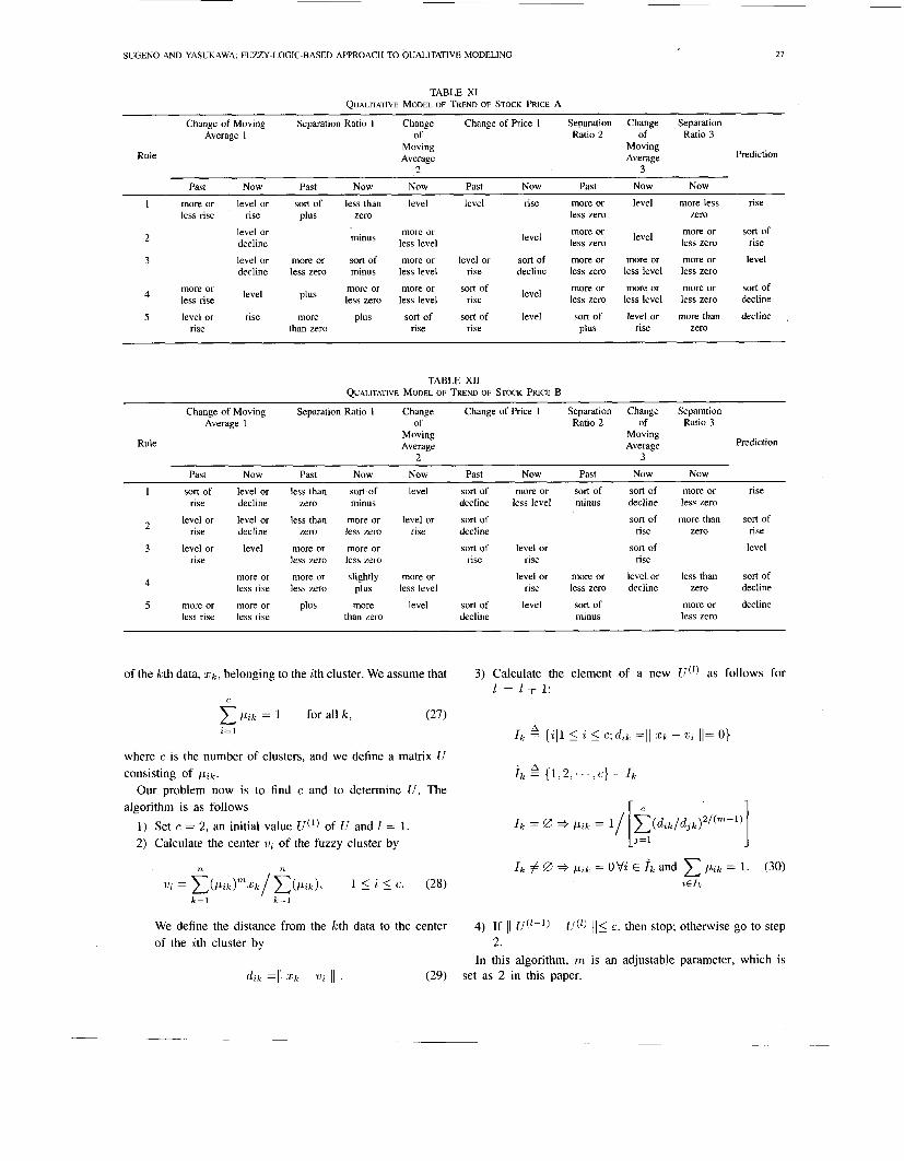
FUZZY VOL. I. A Fuzzy-Logic-Based Approach to Qualitative ...lEEE TRANSACTIONS ON FUZZY SYSTEMS,...

lEEE TRANSACTIONS ON FUZZY SYSTEMS, VOL. I, NO. I . FEBRUARY 1993

A Fuzzy-Logic-Based Approach to Qualitative Modeling

Michio Sugeno and Takahiro Yasukawa

Abstract- This paper discusses a general approach to qualitative modeling based on fuzzy logic. The method of qualitative modeling is divided into two parts: fuzzy modeling and linguistic approximation. It proposes to use a fuzzy clustering method (fuzzy c-means method) to identify the structure of a fuzzy model. To clarify the advantages of the proposed method, it also shows some examples of modeling, among them a model of a dynamical process and a model of a human operator’s control action.

I. INTRODUCTION

N this paper we discuss a method of qualitative modeling I based on fuzzy logic. Related terminologies for qualitative modeling in fuzzy theory are known as fuzzy modeling and linguistic modeling. Qualitative modeling is not so popular in general but this concept is indirectly implied by fuzzy modeling or linguistic modeling. Here we deal with a qualitative model as a system model based on linguistic descriptions just as we use them in sociology or psychology.

Though the terminology of “linguistic modeling” may be straightforward and more appropriate, we use “qualitative modeling” partly because we like to discuss certain problems in comparison with the “qualitative reasoning” approach in artificial intelligence and also because “qualitative modeling” has been one of the most important issues since the very beginning of fuzzy theory. Here artificial intelligence will be abbreviated to AI as usual and the terminology “fuzzy modeling” will be used in a narrow sense.

Before entering the main subject we give an overview of fuzzy modeling in fuzzy theory and qualitative reasoning in AI; then we state the problems concerning qualitative modeling based on fuzzy logic from a systems theory point of view.

After these discussions, we propose a method of qualitative modeling in a general framework known as the black box approach in systems theory. That is, we build a qualitative model of a system without LI priori knowledge about a system provided that we are given numerical input-output data.

A. F i i p Modeling

Though the term “fuzzy modeling” has not been used so often, fuzzy modeling is the most important issue in fuzzy logic or more widely in fuzzy theory. In fact we can find

Manuscript received August 2, 1991; revised April 12, 1992. M. Sugeno is with the Department of Systems Science, Tokyo lnatitute of

Technology, 4259 Nagatauta. Midoriku, Yokohama 227, Japan. T. Yasukawa is with the Department of Control Engineering, Tokyo lnstitutc

of Technology, 4259 Nagatauta, Midoriku, Yokohama 227, Japan. IEEE Log Number 9205336.

the seminal ideas of fuzzy modeling in the early papers of Zadeh. Thus the research concerned with fuzzy niodeling has a history of more than 20 years. There are many interpretations of fuzzy modeling. For instance, we can consider a fuzzy set as a fuzzy model of a human concept. In this study, we simply understand the fuzzy modeling to be an approach to form a system model using a description language based on fuzzy logic with fuzzy predicates. In a broader sense we can interpret the fuzzy modeling as a qualitative modeling scheme by which we qualitatively describe system behavior using a natural language. The fuzzy modeling in a narrow sense is a system description with fuzzy quantities. Fuzzy quantities are expressed in terms of fuzzy numbers or fuzzy sets associated with linguistic labels where a fuzzy set usually does not have a tight relation with a linguistic label; either a fuzzy number does not need to have a linguistic interpretation or a linguistic label is expressed as if it were a frill of a membership function.

On the other hand, what we mean by a qualitative model is a generalized fuzzy model consisting of linguistic explanations about system behavior. Linguistic terms in linguistic explanations are found such that they linguistically approximate the fuzzy sets in an underlying fuzzy model. Furthermore, when a relation of state variables in a system is to be expressed linguistically in a qualitative model, we can use a method of linguistic approximation to accomplish this aim.

In this paper, we focus our attention on qualitative modeling since we want to stress that one of the final targets of fuzzy modeling is “qualitative modeling.” We could even say that fuzzy sets and/or fuzzy logic were suggested with qualitative modeling in mind.

Let us go back to Zadeh’s early ideas. In his paper in 1968 [ I ] following the first paper, “Fuzzy Sets.” in 1965, he suggested using an idea of fuzzy algorithm such as

a) set y approximately equal to I O if .I’ is approximately

b) if .I‘ is large. increase l/J by several units. Those fuzzy algorithms are nothing but qualitative descrip-

tions of a human action, or decision making. As examples, he shows cooking recipes, directions for repairing a TV set, instructions on how to treat a disease, and instructions for parking a car. As for the necessity of fuzzy algorithms, he notes that “most realistic problems tend to be complex, and many complex problems are either algorithmically unsolvable or, if solvable in principle, are computationally infeasible.”

The most remarkable paper related to qualitative modeling is his paper of 1973 [21 on linguistic analysis, where he states ”the principle of incompatibility,” according to which “as the

equal to 5;

1063-6706/93$03 00 G 1993 IEEE

8 IEEE TRANSACTIONS ON FUZZY SYSTEMS, VOL. I , NO. I , FEBRUARY 1993

Case Condition Action to be taken complexity of a system increases, our ability to make precise and yet significant statements about its behavior diminishes until a threshold is reached beyond which precision and significance (or relevance) become almost mutually exclusive

BZ low When BZ is drasticall low:

Ox low (b) reduce fuel BE low

(a) reduce klln s p e J 1

characteristics. It is in this sense that precise quantitative analyses of the behavior of humanistic systems are not likely

When Br is sli htly low: (c) increase I.%. speed (d) decrease fuel rate

to have much relevance to the real world societal, political, economic, and other types of problems which involve humans either as individuals or in groups.”

BZ IOW (a) reduce klln speed Ox low BE O.K.

(b) reduce fuel rate (c) reduce 1. D. fan speed

2

Based on the above considerations Zadeh suggested linguistic analysis in place of quantitative analysis. If we look at his idea of linguistic analysis from the viewpoint of modeling, it is seen to be precisely qualitative modeling. As the main characteristics of this approach, he suggests “1) use of so-called linguistic variables in place of or in addition to numerical variables; 2 ) characterization of simple relations between variables by conditional fuzzy statements; and 3) characterization of complex relations by fuzzy algorithms.”

It is well-known that, motivated by these ideas of “fuzzy algorithm” and “linguistic analysis,” Mamdani first applied fuzzy logic to control [3]. This topic has come to be known as fuzzy algorithmic control or linguistic control. Fuzzy control can be viewed in a certain sense as the result of the qualitative modeling of a human operator working at plant control. For example, fuzzy control rules may be as follows:

1) if the error is positive big and the change of error is positive medium, then the change of control is positive big;

2 ) if the error is positive small and the change of error is positive small, then the change of control is zero,

where the error is the difference between the reference input and the plant output, the change of error is the derivative of the error, and the change of control is the derivative of the control input.

As seen in the above example, we use, to describe control rules, linguistic variables which take linguistic values such as “positive big,” “positive medium,” “zero,” and “negative small.” These are not merely symbols but rather the linguistic labels with quantitative semantics given by underlying fuzzy sets which are associated with membership functions. So we may call a label “positive big” a fuzzy quantity. In fact we use sometimes the term “fuzzy number” or “fuzzy interval.”

The main problem of fuzzy control is to design a fuzzy controller where we usually take an expert-system-like approach. That is, we derive fuzzy control rules from a human operator’s experience and/or engineer’s knowledge, which are mostly based on their qualitative knowledge of an objective system.

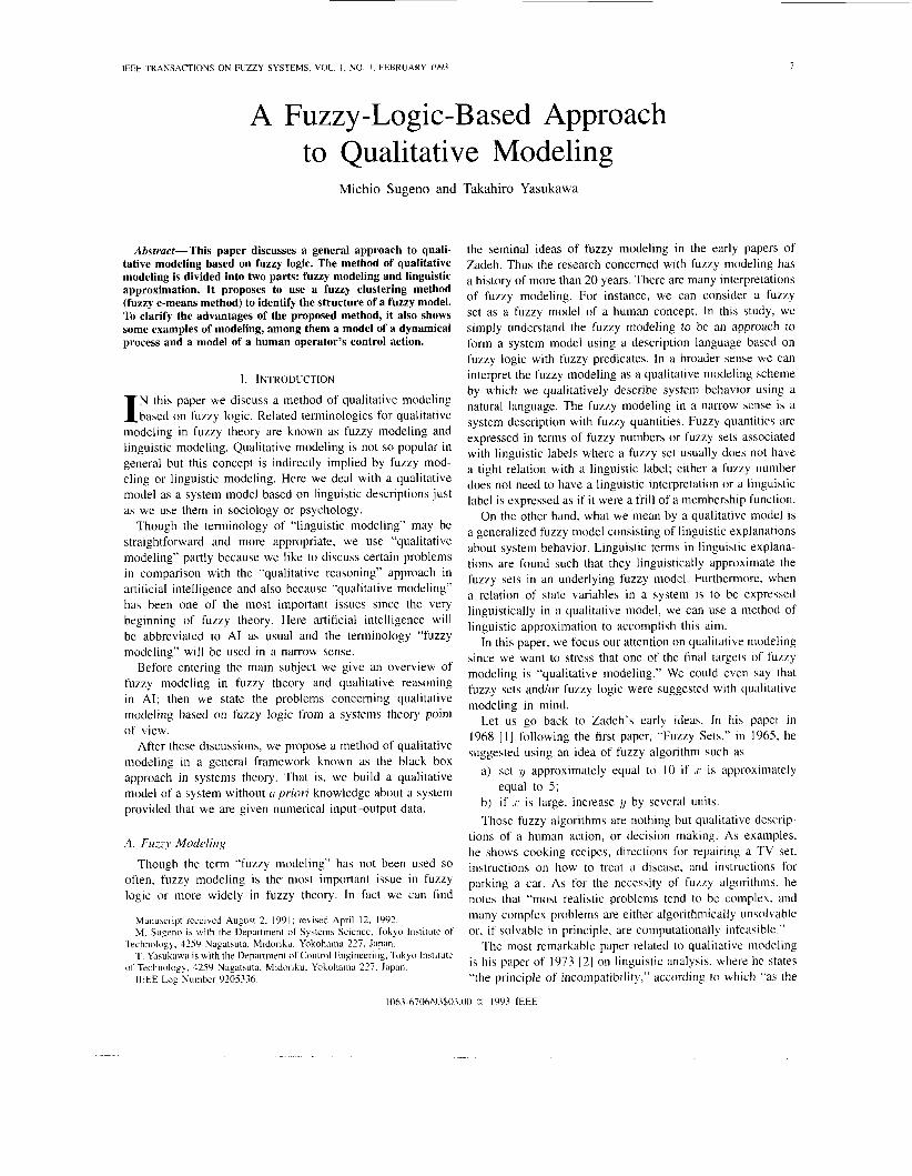
The design procedure is thus something like the following: first, we build linguistic control rules; second, we adjust the parameters of fuzzy sets by which the linguistic terms in the control rules are quantitatively interpreted. For example, let us look at the linguistic rules for controlling a cement kiln [4], as shown in Fig. 1. From these, we can easily derive fuzzy control rules. In this sense, we may say that a set of fuzzy control rules is a linguistic model of human control actions which is not based on a mathematical description of

BZ low a reduce kiln speed Ox low [b] reduce fuel rate

(c) reduce 1. D. fan speed

3

BE high

BE = back end temperature, BZ = burning zone temperature, OX= percentage of oxygen gas In kiln exit gas. Total of 27 rules.

Fig. 1. Operator’s manual of cement kiln control.

human control actions but is directly based on a human way of thinking about plant operation.

Apart from fuzzy control, we have many studies on fuzzy modeling. Those are divided in two groups. The studies of the first group deal with fuzzy modeling of a system itself or a fuzzy modeling for simulation [5]-[8]. Some of those are considered as examples of qualitative modeling. The studies of the second group deal with fuzzy modeling of a plant for control [9]-[13]. Just as with the modem control theory, we can design a fuzzy controller based on a fuzzy model of a plant if a fuzzy model can be identified. Fuzzy modeling in the latter sense is not necessarily viewed as qualitative modeling unless the derivation of a qualitative model from the identified fuzzy model is discussed. It is, of course, quite interesting to derive qualitative control rules based on the qualitative model of a plant.

For example [14], assume that we have a dynamical plant model such as

1) if u , ~ is positive and yn-l is positive, then y, is positive big;

2 ) if U,, is negative and yn-l is positive, then yn is positive small;

3) if U , is positive and yn-l is negative, then yn is negative small;

4) if U , is negative and yn-l is negative, then yn is negative big.

Then given a reference input 7‘ = 0, we can derive the following control rules based on the above model:

1 ) if y,,-1 is positive and y,, is positive big, then U,, is

2 ) if yla-1 is positive and y,, is negative, then U,, is positive; 3) if yTa-l is negative and yn is positive, then ’uTL is

negative; 4) if y,,-1 is negative and yT2 is negative big, then U,, is

positive big. Here the error e,, is equal to -yn since the reference input (the set point) is zxo .

In the fuzzy modeling, the most important problem is the identification method of a system. The identification for the

negative big;

SUGENO AND YASUKAWA: FUZZY-LOGIC-BASED APPROACH TO QUALITATIVE MODELING

fuzzy modeling has two aspects as usual: structure identification and parameter identification. This problem will be discussed in subsection D.

E. Qualitative Reasoning

Outside the research area of fuzzy logic, the concept of qualitative reasoning has been suggested in AI. Earlier studies of qualitative reasoning were found on mechanical systems in 1975 [15], and also on naive physics in 1979 [16]. We can identify as typical studies of qualitative reasoning the following:

1) qualitative physics or naive physics [ 171, 2 ) qualitative process theory [ 181, 3) qualitative simulation [ 191. Here we call these ideas qualitative reasoning. The aims and

characteristics of qualitative reasoning may be summarized as follows. According to de Kleer [17], “the behavior of a physical system can be discussed by the exact values of its variables (forces, velocities, positions, pressures, etc.) at each time instant. Such a description, although complete, fails to provide much insight into how the system functions. Our long- temi goal is to develop an alternate physics in which these same concepts are derived from a far simpler, but never the less formal qualitative basis . . . our proposal is to reduce the quantitative precision of the behavioral descriptions but retain the crucial distinctions.”

Also if we refer to Kuipers [ 191, we find “an expert system is often a shallow model of its application domain, in the sense that conclusions are drawn directly from observable features of the presented situation. One major line of research toward the representation of deep models is the study of qualitative causal models. Research on qualitative causal models differs from more general work on deep models in focusing on qualitative descriptions of the deep mechanism, capable of representing incomplete knowledge of the structure and behavior of the mechanism.”

As we find in the above statements, there are small distinctions and big similarities between fuzzy modeling and qualitative reasoning. One distinction is that fuzzy modeling starts from the fact that a precise mathematical model of a complex system cannot be obtained, whereas qualitative reasoning starts from the fact that, although a complete model may be available, i t cannot provide insight into the system; a description based on deep knowledge is needed. On the other hand, similarities are found in the confidence of the advantage of qualitative expressions, in the goals, and in some parts of description languages for modeling. The common idea of qualitative system theory should be emphasized.

Qualitative reasoning makes use of a quantity space on which “landmarks” are defined. Usually one landmark “0” is set, and then three values {+. 0 . - } are used which are qualitative in nature, similar to fuzzy values {positive, zero, negative} in fuzzy modeling. The difference between them is that qualitative values are crisp, acting as symbols, though they call {+. 0 . - } semantics, while fuzzy values are not symbols but quantitative semantics represented by their membership functions. In qualitative reasoning such phenomena as

1) temperature c( Q+ pressure 2 ) pressure x Q- volume

1) if the temperature increases (decreases), then pressure

2) if pressure increases (decreases), then volume decreases

As we have seen, this sort of description was found in Zadeh’s paper in 1968, which shows our motivation to use fuzzy concepts. As far as reasoning is concemed, in qualitative reasoning the following arithmetic is defined:

are interpreted as

increases (decreases);

(increases).

[:J; X y] = [:I;] X

where [ x ] means a qualitative value of a physical quantity .r. n is a discrete time, and i3.r is the qualitative derivative of .I’ with the values of {+. 0. -} . Equations ( I ) and ( 2 ) describe binary operations on qualitative values; (3) describes the dynamical relation of a system.

We must point out that, in fuzzy theory, the arithmetic of fuzzy numbers is in a much more general setting. For example we have

where n, is a fuzzy number, “approximately U,’’ associated with

a membership function, e.g.,

The arithmetic in (4) and ( 5 ) is a generalization of the ordinary arithmetic, which of course precisely includes ( 1 ) and ( 2 ) .

In fuzzy modeling, the fuzzy arithmetic is used for com- putation and “if-then rules” are used for inference together with fuzzy reasoning based on fuzzy logic. Fuzzy reasoning is interpreted as approximate reasoning based on vague or incomplete knowledge.

As far as the tools for model description are concerned, those in qualitative reasoning seem to be very simple compared with those in fuzzy modeling. We can recall a dentist’s way of description: a dentist uses the symbols {++. +. i. -. - -}, and a control engineer uses in the bang-bang control the symbols {+l. -l}, where the symbol zero can be added as an ideal case in the middle of + I and - I from a theoretical point of view. The dentist’s symbols are fuzzy in nature, much more similar- to fuzzy values, while the control symbols are crisp and look similar to qualitative reasoning.

Now let us look at the basic approach of qualitative modeling. As far as the authors can determine, this approach suggests I ) to make a model by observations of phenomena based on,

in IEEE TRANSACTIONS ON FUZZY SYSTEMS, VOL. I , NO. I , FEBRUARY 1993

for instance, empirical and/or physical knowledge or 2) to derive a qualitative model based on a differential equation of a system. This approach is effective if a system is simple, for example a mechanical system with a small number of state variables and simple interactions among state variables. But, of course, even if a system is composed of many state variables, this approach is useful provided that the system is a lumped- parameter system such as an electric circuit. As a conclusion it seems that qualitative modeling is concerned with well- structured systems; in most studies on qualitative modeling, they deal with toy systems, if we look at those from a systems

2) If z1 is small and z 2 is more or less small or medium small, then y is big, dy/dzl is very negative, and dy/dxz is very negative.

We can regard most of fuzzy models and fuzzy control rules [24], [25] as qualitative models.

We distinguish, however, in this paper, a qualitative model from a fuzzy model. The terminology “a fuzzy model” is used in a narrow sense. A qualitative model is considered a fuzzy model with something more, i.e., with more linguistic expressions.

For example, a fuzzy model of the type 1) if z is approximately 3, then y is approximately 5; theory point of view.

First of all, if a mathematical model is available, we can use it for the purpose of engineering (analysis, control and prediction). This fact of course does not prevent us for making a qualitative model of a system, for instance, in order to explain its general structure and behavior to students.

Second, even if we can find the local mechanisms of a system, it is often the case that we cannot build the whole system

In modeling we do not take this approach to 2) if z increases by approximately 5, then y decreases by approximately 4

should not be called a qualitative model. We can call the above model a fuzzy number model to distinguish it from a qualitative model.

Further, in an ordinary fuzzy model that is used in fuzzy control such as

mode] by aggregating the local mechanisms. This is why we l ) if is positive then is negative take a so-called black box approach to Systems identification 2, if is positive medium, then !/ is positive _ _ in systems engineering. We have to note that what we mean by a complex system is a system for which we cannot have a relevant mathematical model; in other words, we cannot build a global system model by integrating local models.

There is another reason for a black box approach. It is often the case that we cannot measure the states of a dynamical system. We can observe only the inputs and the outputs of a system in many cases.

Summing up the above the discussions on qualitative reasoning and fuzzy modeling, we may conclude: l ) motivations are different, 2) goals look similar, 3) tools are much more powerful in fuzzy modeling, and 4) methods of approach to modeling are different and those in fuzzy modeling are more varied and applicable. In any case, however, we see similarities between qualitative reasoning and fuzzy modeling rather than differences.

The research domain of fuzzy logic started adopting a qualitative approach to systems analysis in the late 1960’s. We are quite sure that fuzzy modeling can be directly applied to problems considered by a qualitative reasoning method. Despite these facts, it is a great pity that we can hardly find any reference to fuzzy logic in the papers related to qualitative reasoning.

C. Qualitative Modeling

What we imply here by a qualitative model [20]-[23] is a linguistic model. A linguistic model is a model that is described or expressed using linguistic terms in the framework of fuzzy logic instead of mathematical equations with numerical values or conventional logical formula with logical symbols. For example as we shall see later, a linguistic model of a two input-single output system is something like the following:

1 ) if .r1 is more than medium and .1‘2 is more than medium. then is small, ag/13.r1 is sort of negative, and t l ,y/ t l ,rz is sort of negative.

the terms “positive small,” “negative small,” etc., are the labels conventionally attached to fuzzy sets, where the fuzzy sets play an important role, not the labels.

We go beyond this stage by utilizing of the concept of “linguistic approximation.” That is, given a conventional fuzzy model with fuzzy sets, we improve its qualitative nature by using linguistic approximation techniques in fuzzy logic. In other words, we deal with a model in which we focus our attention on how to linguistically or qualitatively explain a system behavior as we shall see in what follows.

Now let us discuss available sources, i.e., information or data, for qualitative modeling. We find the following classification of the sources:

1) conventional mathematical models 2) observation based on knowledge and/or experience 3) numerical data 4) image data 5 ) linguistic data.

In qualitative reasoning as we have seen, a model is built based on 1) and 2). A conventional mathematical model is usually identified based on 2) and 3). A fuzzy model is also based on 2) and 3), as in the case of a mathematical model. Sources 4) and 5 ) are also useful to build a qualitative model. A qualitative model based on 4), image data, can be interpreted as image understanding, that is, a linguistic explanation of an image. As for the examples concerned with 5 ) , we can consider translation of one language into another or making a summary of a story.

In this paper we deal with qualitative modeling based partly on 2) and mainly on 3), as usual; a black box approach. The reason for this is that system identification is a key issue in the black box approach and all the basic matters in model building appear in the context of system identification. Indeed we think that any method of modeling should be able to solve the problems discussed from now on.


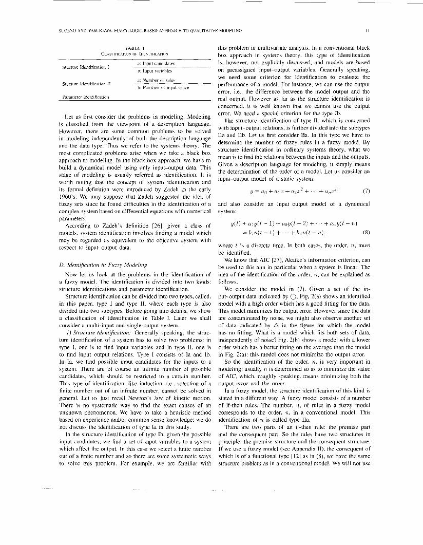
TABLE I CLASSIFICATION OF IDENTII-ICATIOV

a: Input candidates b: Input variables

Stucture Identification I

a: Number of rules b: Partition of input space

Stucture Identification I1

Parameter identification

Let us first consider the problems in modeling. Modeling is classified from the viewpoint of a description language. However, there are some common problems to be solved in modeling independently of both the description language and the data type. Thus we refer to the systems theory. The most complicated problems arise when we take a black box approach to modeling. In the black box approach, we have to build a dynamical model using only input-output data. This stage of modeling is usually referred as identification. It is worth noting that the concept of system identification and its formal definition were introduced by Zadeh in the early 1960's. We may suppose that Zadeh suggested the idea of fuzzy sets since he found difficulties in the identification of a complex system based on differential equations with numerical parameters.

According to Zadeh's definition [26], given a class of models, system identification involves finding a model which may be regarded as equivalent to the objective system with respect to input-output data.

D. Identification in Fuzzy Modeling

Now let us look at the problems in the identification of a fuzzy model. The identification is divided into two kinds: structure identifications and parameter identification.

Structure identification can be divided into two types, called, in this paper, type I and type 11, where each type is also divided into two subtypes. Before going into details, we show a classification of identification in Table I. Later we shall consider a multi-input and single-output system.

I ) Structure Identijkation: Generally speaking, the structure identification of a system has to solve two problems: in type I, one is to find input variables and in type 11, one is to find input-output relations. Type I consists of Ia and Ib. In Ia, we find possible input candidates for the inputs to a system. There are of course an infinite number of possible candidates, which should be restricted to a certain number. This type of identification, like induction, i.e., selection of a finite number out of an infinite number, cannot be solved in general. Let us just recall Newton's law of kinetic motion. There is no systematic way to find the exact causes of an unknown phenomenon. We have to take a heuristic method based on experience andlor common sense knowledge; we do not discuss the identification of type Ia in this study.

In the structure identification of type Ib, given the possible input candidates, we find a set of input variables to a system which affect the output. In this case we select a finite number out of a finite number and so there are some systematic ways to solve this problem. For example, we are familiar with

this problem in multivariate analysis. In a conventional black box approach in systems theory, this type of identification is, however, not explicitly discussed, and models are based on preassigned input-output variables. Generally speaking, we need some criterion for identification to evaluate the performance of a model. For instance, we can use the output error, i.e., the difference between the model output and the real output. However as far as the structure identification is concerned, it is well known that we cannot use the output error. We need a special criterion for the type Ib.

The structure identification of type 11, which is concerned with input-output relations, is further divided into the subtypes IIa and IIb. Let us first consider IIa. In this type we have to determine the number of fuzzy rules in a fuzzy model. By structure identification in ordinary systems theory, what we mean is to find the relations between the inputs and the outputs. Given a description language for modeling, it simply means the determination of the order of a model. Let us consider an input-output model of a static system:

,y = a[) + fL1.l ' + f L * 2 + . ' ' + U I 1 ' I.'L (7)

and also consider an input-output model of a dynamical system:

where f is a discrete time. In both cases, the order, i t , , must be identified.

We know that AIC [27], Akaike's information criterion, can be used to this aim in particular when a system is linear. The idea of the identification of the order, 71, can be explained as follows.

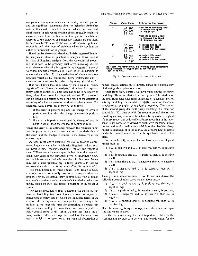
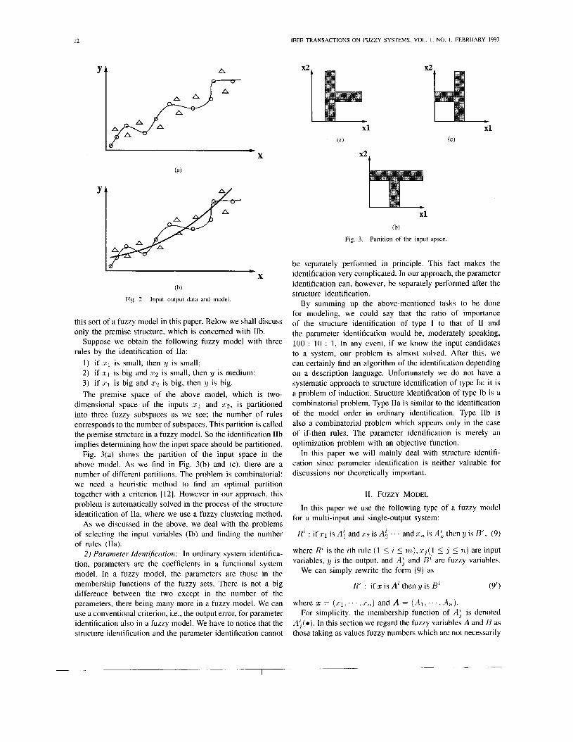
We consider the model in (7). Given a set of the input-output data indicated by 0, Fig, 2(a) shows an identified model with a high order which has a good fitting for the data. This model minimizes the output error. However since the data are contaminated by noise, we might also observe another set of data indicated by A in the figure for which the model has no fitting. What is a model which fits both sets of data, independently of noise? Fig. 2(b) shows a model with a lower order which has a better fitting on the average than the model in Fig. 2(a): this model does not minimize the output error.

So the identification of the order, i i , is very important in modeling: usually 'rt is determined so as to minimize the value of AIC, which, roughly speaking, means minimizing both the output error and the order.

In a fuzzy model, the structure identification of this kind is stated in a different way. A fuzzy model consists of a number of if-then rules. The number, 71, of rules in a fuzzy model corresponds to the order, n, in a conventional model. This identification of 71 is called type IIa.

There are two parts of an if-then rule: the premise part and the consequent part. So the rules have two structures in principle: the premise structure and the consequent structure. If we use a fuzzy model (see Appendix II) , the consequent of which is of a functional type [ 121 as in (8), we have the same structure problem as in a conventional model. We will not use

12

A i.-l.I'- IEEE TRANSACTIONS ON FUZZY SYSTEMS, VOL. I , NO. I . FEBRUARY 1993

(b)

Fig. 2 . Input+utput data and model

this sort of a fuzzy model in this paper. Below we shall discuss only the premise structure, which is concerned with IIb.

Supposz we obtain the following fuzzy model with three rules by the identification of IIa:

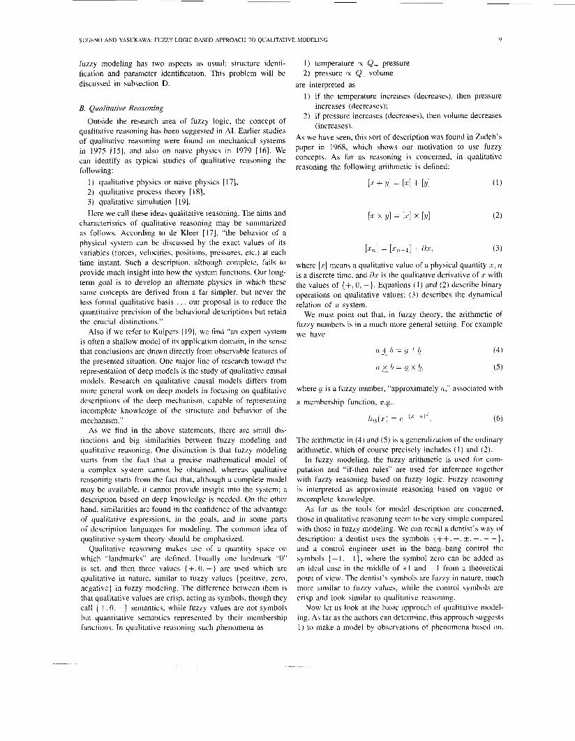
1 ) if 5 1 is small, then y is small; 2 ) if 5 1 is big and z 2 is small, then y is medium; 3) if x:1 is big and 2 2 is big, then y is big. The premise space of the above model, which is two-

dimensional space of the inputs 2 1 and 5 2 , is partitioned into three fuzzy subspaces as we see; the number of rules corresponds to the number of subspaces. This partition is called the premise structure in a fuzzy model. So the identification IIb implies determining how the input space should be partitioned.

Fig. 3(a) shows the partition of the input space in the above model. As we find in Fig. 3(b) and (c), there are a number of different partitions. The problem is combinatorial: we need a heuristic method to find an optimal partition together with a criterion [ 121. However in our approach, this problem is automatically solved in the process of the structure identification of IIa, where we use a fuzzy clustering method.

As we discussed in the above, we deal with the problems of selecting the input variables (Ib) and finding the number of rules (Ha).

2) Parameter Identijication: In ordinary system identification, parameters are the coefficients in a functional system model. In a fuzzy model, the parameters are those in the membership functions of the fuzzy sets. There is not a big difference between the two except in the number of the parameters, there being many more in a fuzzy model. We can use a conventional criterion, i.e., the output error, for parameter identification also in a fuzzy model. We have to notice that the structure identification and the parameter identification cannot

xl

xl (b)

Fig. 3. Partition of the input space.

be separately performed in principle. This fact makes the identification very complicated. In our approach, the parameter identification can, however, be separately performed after the structure identification.

By summing up the above-mentioned tasks to be done for modeling, we could say that the ratio of importance of the structure identification of type I to that of I1 and the parameter identification would be, moderately speaking, 100 : 10 : 1. In any event, if we know the input candidates to a system, our problem is almost solved. After this, we can certainly find an algorithm of the identification depending on a description language. Unfortunately we do not have a systematic approach to structure identification of type Ia: it is a problem of induction. Structure identification of type Ib is a combinatorial problem. Type IIa is similar to the identification of the model order in ordinary identification. Type IIb is also a combinatorial problem which appears only in the case of if-then rules. The parameter identification is merely an optimization problem with an objective function.

In this paper we will mainly deal with structure identification since parameter identification is neither valuable for discussions nor theoretically important.

11. FUZZY MODEL

In this paper we use the following type of a fuzzy model

R' : if :c1 is Ai and :1:2 is Ai . . . and xTt is Ai, then y is Bi . (9)

where R' is the %th rule (1 5 i 5 vi), x:j( 1 5 j 5 71) are input variables, :I/ is the output, and Ai and B' are fuzzy variables.

for a multi-input and single-output system:

We can simply rewrite the form (9) as

R' : if z. is Ai then TJ is Bi (9')

where z = (XI.. . . . : r T l ) and A = ( A I , . . . . A 7 , ) . For simplicity, the membership function of AS is denoted

Ai (e) . In this section we regard the fuzzy variables A and B as those taking as values fuzzy numbers which are not necessarily


~

13

associated with linguistic labels. Our method of qualitative modeling consists of two steps. In the first step we deal with a fuzzy model in terms of fuzzy numbers. In the second step we give linguistic interpretations to this fuzzy model. That is, we deal with a fuzzy model with linguistic terms which we call a qualitative model. Occasionally we let BZ take singletons, i.e., real numbers, instead of fuzzy numbers. As far as fuzzy control is concerned, it is well known that we can use fuzzy rules with singletons in the consequents without losing the performance of the control. However in order to derive a qualitative model from the fuzzy model in (9), it is better to use fuzzy numbers in the consequents.

As for reasoning, we modify partly the ordinary method as seen in the following steps 2) and 3):

1) Given the inputs xy. x! , . . . , and x:, calculate the degree of match, wi, in the premises for the ith rule, 1 5 i 5 m as

W' = A",z:) x A;( :E~) x . . . x Ak(z:). (10)

2) Then defuzzify Bz in the consequents by taking the center of gravity:

b2 = 1 B'(Y)&/ J' B"Y)4!. ( 1 1 )

3) Calculate the inferred value, ij, by taking the weighted average of ba with repsect to uf

m I 111 ...

i = l i=l

where m is the number of rules. As we find in the process of reasoning, the rule Ra translate

(13)

In what follows we shall call a fuzzy model in the form (9) a position type model.

Next we propose occasionally to use a position-gradient type model. It is often the case that we cannot build a fuzzy model over the whole input space because we lack data. In this case we need to take an extrapolation for estimating the output using local fuzzy rules. Note that in conventional fuzzy reasoning we take an interpolation using some number of rules.

to the form

R' : if z IS A' then y is b'.

A position-gradient model is of the following form:

R' : if z is A' then y is B' and d!g/i)z is C'. (14)

where ay/dz = (ay/a.rl.. . . . t l ! ~ / t l . r , ~ ) . C' = (Ci. . . . . C;L). and a y / a ~ ~ is the partial derivative of y with respect to , rJ .

Using the rules shown in (14), we can infer the output for a given input for which no rule of the position type is available; if w' = 0 in all the rules for the inputs, 4 cannot be inferred in the position type model. The reasoning algorithm of the position-gradient rules is the following:

1 ) Defuzzify B' and C', and let those values be b' and c', respectively, where c' = ( r i . . . . . ( . i t ) . We can rewrite (13) as

R' : if z is A' then y is b' and a*y/az is c' . ( 15)

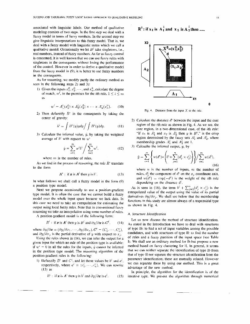
Ri:ifxlis Aiand x 2 isA2then i .....

, ,

m 0

Fig. 4. Distance from the input S to the rule.

2) Calculate the distance di between the input and the core region of the ith rule as shown in Fig. 4. As we see, the core region, in a two-dimensional case, of the ith rule: "if 5 1 is Ai and z2 is Ai then y is BZ," is the crisp region determined by the fuzzy sets Ai and A i , where membership grades Ai and Ai are 1.

3) Calcualte the inferred output, y, by

i j = m { l lI(di)* (hi+@ x c # ~ 7 1 1 ( d i ) ,

i = l i=l

(16) where 71 is the number of inputs, m the number of rules, d i the component of di on the x j coordinate axis, and rw(d2) = e x p ( - d i ) is the weight of the ith rule dependeing on the distance d' .

As is seen in (16), the term bz + x,"=,(dj x e:) is the extrapolated value of the output using the value of its partial derivatives ay/dz j . We shall see below that the membership functions in this study are almost always of a trapezoidal type as shown in Fig. 4.

A. Structure Identification

Let us now discuss the method of structure identification. As stated in the Introduction we have to deal with structures of type Ib: to find a set of input variables among the possible candidates, and with structures of type 11: to find the number of rules and a fuzzy partition of the input space (see Table I). We shall use an ordinary method for Ib but propose a new method based on fuzzy clustering for 11. In general, it seems that we can neither separate the identification of type Ib from that of type I1 nor separate the structure identification from the parameter identification; these are mutually related. However we can separate these by using our method. This is a great advantage of the new method.

In principle, the algorithm for the identification is of the iterative type. We present the algorithm through numerical


1.31 3.35 2.10 3.52 2.46 1.95 2.51 2.70 1.33 4.63 2.80 1.97 2.47 2.66 2.08 2.75 1.51 2.40 2.44 1.99 3.42 4.99 2.27 3.94

TABLE I1 INPUT-OUTPUT DATA OF NONLINEAR SYSTEM

27 28 29 30 31 32 33 34 35 36 37 38 39 40 41 42 43 44 45 46 47 48 49 50

1

2 3 4 5 6 7 8 9 I O 1 1

12 13 14 15 16 17 18 19 20 21 22 23 24 25

1.40 4.28 1.18 1.96 1.85 3.66 3.64 4.5 1

3.77 4.84 1.05 4.5 1

1.84 1.67 2.03 3.62 1.67 3.38 2.83 I .48 3.37 2.84 1.19 4.10 1.65

1.80 4.96 4.29 1.90 1.43 1.60 2.14 1.52 1.45 4.32 2.55 1.37 4.43 2.8 1 I .88 I .95 2.23 3.70 1.77 4.44 2.13 1.24 1.53 1.71 1.38

3.00 3.02 1.60 1.71 4.15 3.44 1.64 4.53 2.50 2.15 3.03 3.97 4.20 2.23 1.41 4.93 3.93 4.65 2.61 1.33 2.42 4.42 2.54 2.54 4.57

3.80 4.39 3.80 I .59 3.30 3.33 2.64 2.54 1.86 1.70 2.02 I .70 I .38 4.5 1 1.10 1.58 1.06 1.28 4.50 3.25 3.95 1.21 3.22 1.76 4.03

Group A Group B

No. .rl .r2 .r2 .r3 Y No. .r 1 .1.2 .r3 .r4 Y

2.71 4.13 4.38 3.21 1.58 1.78 1.11 3.13 1.80 4.71 3.61 2.27 2.27 3.61 1.87 2.24 3.74 4.25 3.26 1.79 1.81 3.18 3.31 2.07 2.20 4.85 4.66 4.1 I 3.74 1.30 3.41 3.88 1.27 2.21 1.48 1.38 2.55 2.07 4.42 3.14 2.46 2.12 1 . 1 1 4.44 2.22 2.66 4.42 1.71 1.23 1.56 4.44 4.71 1.53 2.08 1.32 3.11 1.06 2.91 2.80 4.08 4.47 3.66 1.23 3.62 1.42 1.35 1.76 3.00 3.82 3.91 1.24 1.41 1.92 2.25 5.05 2.81 1.35 4.96 4.04 1.97 1.92 4.25 3.24 3.89 1.92 4.61 2.68 4.89 1.03 1.63 3.04 4.97 2.77 2.63 1.44 4.82 3.80 4.73 2.69 1.39 2.58 1.97 4.16 2.95 2.29 4.14 4.76 2.63 3.88 1.33 4.35 3.90 2.55 1.65 1.40 2.22 1.35 2.75 1.01 3.39

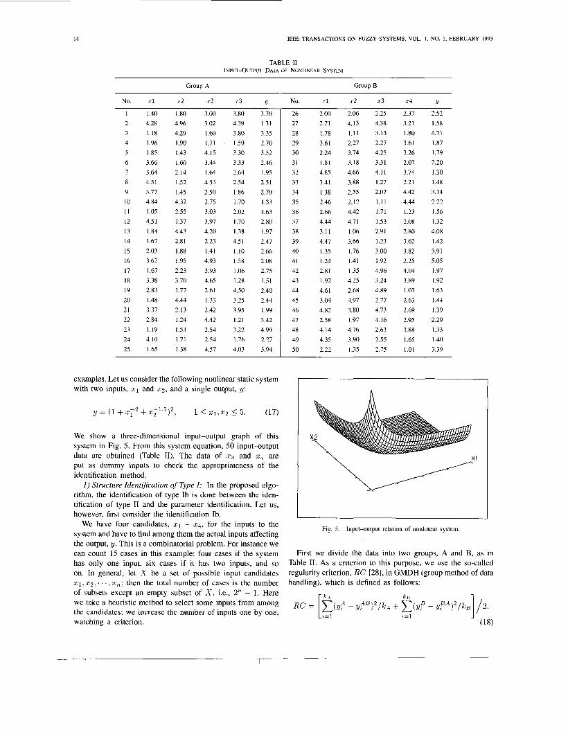
examples. Let us consider the following nonlinear static system with two inputs, x1 and 2 2 , and a single output, y:

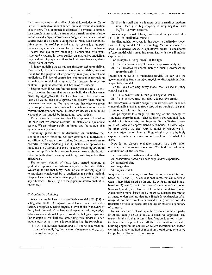
We show a three-dimensional input-output graph of this system in Fig. 5. From this system equation, 50 input-output data are obtained (Table 11). The data of 2 3 and x4 are put as dummy inputs to check the appropriateness of the identification method.

1 ) Structure IdentGcation of Type I: In the proposed algorithm, the identification of type Ib is done between the identification of type I1 and the parameter identification. Let us, however, first consider the identification Ib.

We have four candidates, 2 1 - ~ 4 , for the inputs to the system and have to find among them the actual inputs affecting the output, y. This is a combinatorial problem. For instance we can count 15 cases in this example: four cases if the system has only one input, six cases if it has two inputs, and so on. In general, let X be a set of possible input candidates 5 1 , 2 2 . . . . . xTL; then the total number of cases is the number of subsets except an empty subset of X , i.e., 2" - 1. Here we take a heuristic method to select some inputs from among the candidates; we increase the number of inputs one by one, watching a criterion.

Fig. 5. Inputboutput relation of nonlinear system.

First we divide the data into two groups, A and B, as in Table 11. As a criterion to this purpose, we use the so-called regularity criterion, RC [28], in GMDH (group method of data handling), which is defined as follows:

k B

- Y ? B ) 2 / h + ELY: - Ip"! ' /kB] / 2 . 1 = l

(18)


~

15

TABLE Ill STRUCTURE IDENTIFICATION Ib OF NONLINEAR SYSTEM

Input RC Variables

.r 1

Step 1 s 2 .r3 .r1

0

0.863 0.830 0.937

. r l - .r2 Step 2

.r l - 1.3

.r l - . x i

.r1 - s2 - .r3

. r l - .rL - .rf Step 3

0.57 I 0.583

0.483 X

0.493 X

where

k 1 and k ~ : the number of data of the groups A and B; the output data of the groups A and B;

the model output for the group A input estimated by the model identified using the group B data; the model output for the group B input estimated by the model identified using the group A data.

y,' and yp:

y IB:

,,B I .

As we can guess from the form of RC, we build two models for two data groups at each stage of the identification. Notice that we have to make the structure identification of type I1 and the parameter identification in order to calculate RC. We can easily find the meaning of RC in Fig. 2.

Now we show the outline of a heuristic algorithm for Ib. First, we begin with a fuzzy model with one input. We make four models: one model for one particular input. After the identification of the structure I1 and parameter identification, which will be described later, we calculate RC of each model and select one model to minimize RC from among the one- input models. Next we fix the one input selected above and add another input to our fuzzy model from among the remaining three candidates. Our fuzzy model has two inputs at this stage. We select the second input as we do at the first step, according to the value of RC.

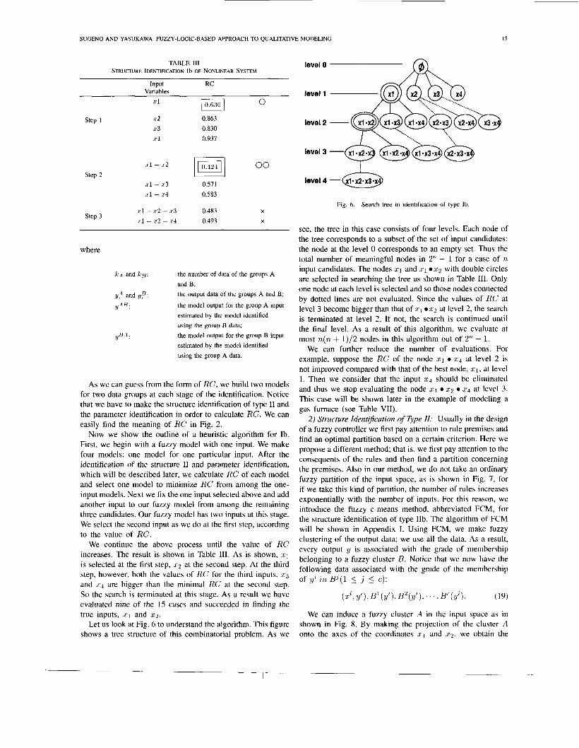
We continue the above process until the value of RC increases. The result is shown in Table 111. As is shown, .c1

is selected at the first step, .r2 at the second step. At the third step, however, both the values of RC for the third inputs, . r ~ and .rA are bigger than the minimal RC at the second step. So the search is terminated at this stage. As a result we have evaluated nine of the 15 case5 and succeeded in finding the true inputs, . r 1 and .r2.

Let us look at Fig. 6 to understand the algorithm. This figure shows a tree structure of this combinatorial problem. As we

level

level

level

level 4 - xl x2 x3 x

Fig. 6. Search tree in identification of type Ib

see, the tree in this case consists of four levels. Each node of the tree corresponds to a subset of the set of input candidates: the node at the level 0 corresponds to an empty set. Thus the total number of meaningful nodes in 2" - 1 for a case of n, input candidates. The nodes 2 1 and ~ 1 . 2 2 with double circles are selected in searching the tree as shown in Table 111. Only one node at each level is selected and so those nodes connected by dotted lines are not evaluated. Since the values of RC at level 3 become bigger than that of :c1 0 2 2 at level 2, the search is terminated at level 2 . If not, the search is continued until the final level. As a result of this algorithm, we evaluate at most n(n + l ) / 2 nodes in this algorithm out of 21L - 1.

We can further reduce the number of evaluations. For example, suppose the RC of the node z1 0 2 4 at level 2 is not improved compared with that of the best node, 1c1, at level 1. Then we consider that the input xq should be eliminated and thus we stop evaluating the node 5 1 0 x2 0 5 4 at level 3 . This case will be shown later in the example of modeling a gas furnace (see Table VII).

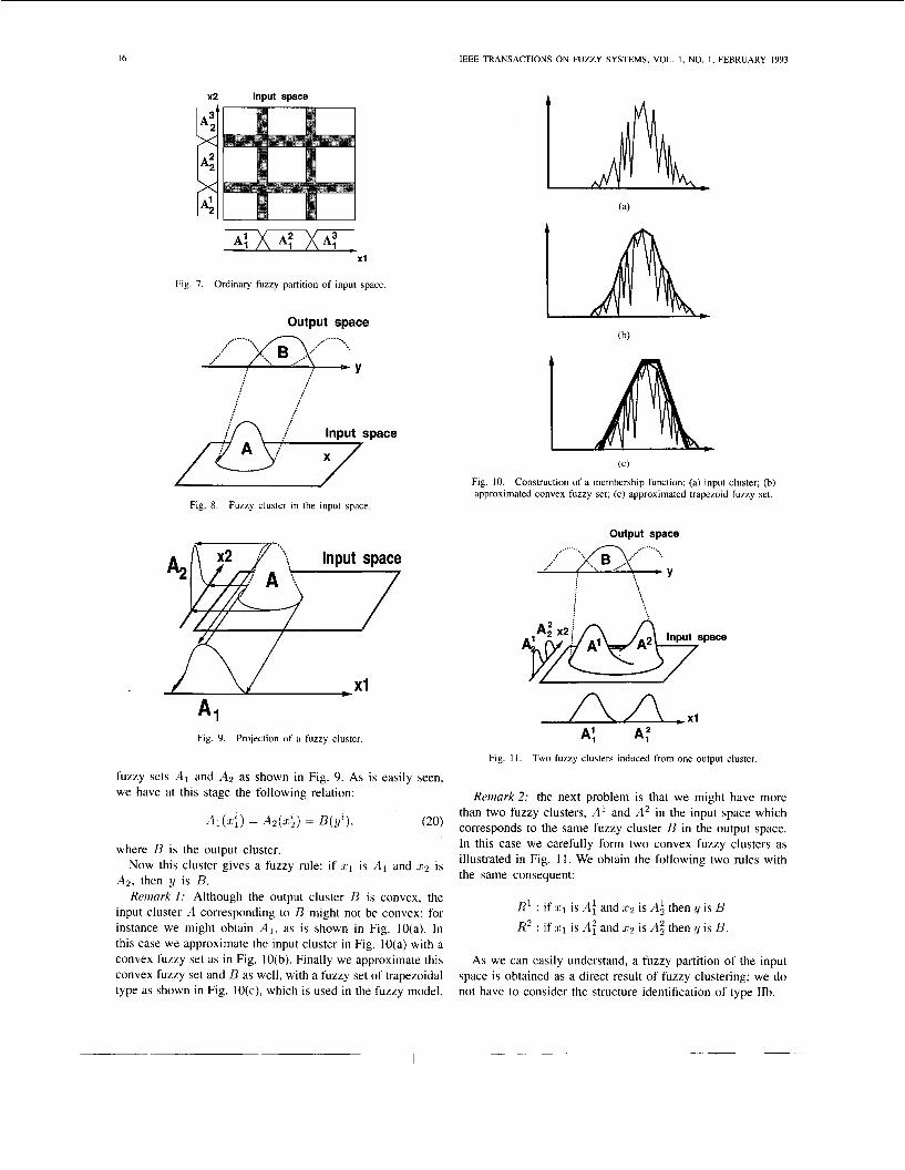
2) Structure ldenrijcation of Dpe II: Usually in the design of a fuzzy controller we first pay attention to rule premises and find an optimal partition based on a certain criterion. Here we propose a different method; that is, we first pay attention to the consequents of the rules and then find a partition concerning the premises. Also in our method, we do not take an ordinary fuzzy partition of the input space, as is shown in Fig. 7, for if we take this kind of partition, the number of rules increases exponentially with the number of inputs. For this reason, we introduce the fuzzy c-means method, abbreviated FCM, for the structure identification of type IIb. The algorithm of FCM will be shown in Appendix I . Using FCM, we make fuzzy clustering of the output data; we use all the data. As a result, every output y is associated with the grade of membership belonging to a fuzzy cluster B. Notice that we now have the following data associated with the grade of the membership of y i ,in BJ(l 5 :j 5 c ) :

We can induce a fuzzy cluster A in the input space as in shown in Fig. 8. By making the projection of the cluster A onto the axes of the coordinates .rl and .r2, we obtain the

~ -- I-- -

16

x2 Input space

X I

Fig. 7. Ordinary fuzzy partition of input space

Output space

IEEE TRANSACTIONS ON FUZZY SYSTEMS, VOL. I , NO. I , FEBRUARY 1993

fi,/ 7 p a c e

X (c)

Fig. IO. Construction of a membership function: (a) input cluster; (b) approximated convex fuzzy set; (c) approximated trapezoid fuzzy set.

Fig. 8. Fuzzy cluster in the input space.

Output space

Fig. 9. Projection of a fuzzy cluster.

fuzzy sets A I and A2 as shown in Fig. 9. As is easily seen, we have at this stage the following relation:

where B is the output cluster. Now this cluster gives a fuzzy rule: if : c 1 is A I and 1c2 is

A2, then :y is B. Remark I : Although the output cluster B is convex, the

input cluster A corresponding to B might not be convex: for instance we might obtain A l , as is shown in Fig. 10(a). In this case we approximate the input cluster in Fig. 10(a) with a convex fuzzy set as in Fig. 10(b). Finally we approximate this convex fuzzy set and B as well, with a fuzzy set of trapezoidal type as shown in Fig. 10(c), which is used in the fuzzy model.

Fig. 1 I . Two fuzzy clusters induced from one output cluster.

Remark 2: the next problem is that we might have more than two fuzzy clusters, A' and A2 in the input space which corresponds to the same fuzzy cluster B in the output space. In this case we carefully form two convex fuzzy clusters as illustrated in Fig. 11 . We obtain the following two rules with the same consequent:

R1 : if : c 1 is A: and z 2 is Ai then ;y is B R 2 : if :rl is A: and L I : ~ is Ai then y is B.

As we can easily understand, a fuzzy partition of the input space is obtained as a direct result of fuzzy clustering; we do not have to consider the structure identification of type IIb.

SUGENO AND YASUKAWA: FUZZY-LOGIC-BASED APPROACH TO QUALITATIVE MODELING 17

-20 1 -21.58

-30 4 \ -32.47

3.66

R’ ; if x l i s m and x2 i s f o then y is 1.70 4.95 1.73 4.97 1.30

1.80 3.60 1.95 4.43

R2; if XI i s [ B and x2 ism then y is rb 1.50 4.80 1.42 4.55 1.51 2.60

I \ 2.00 4.50 1.52 4.43 2.51 2.66

-41.69 R3; if x l ism and x2 i s g then y is 1.53 3.31 0.91 7.97 + 0.50 4.60

1.18 2.84 1.24 4.29 -42.70

Fig. 12. Behavior of S ( c ) in nonlinear system model.

Let us discuss a method to determine the number of rules which is related to the number of fuzzy clusters in fuzzy clustering. Note that, because of Remark 2 the number of fuzzy rules is not exactly the same as that of fuzzy clusters in the output space, as we have just discussed above.

The determination of the number of clusters is the most important issue in clustering. There are many studies on this issue [29]-[31]. Here we use the following criterion [31] for this purpose:

n c

k l i=l

where

U : number of data to be clustered; c: number of clusters, c 2 2; ,rh.: kth data, usually vector; .r: average of data: s 1. .r2 . . . .rrz ;

: vector expressing the center of ith cluster;

11 . 11: n o m ;

p L k :

111:

grade of kth data belonging to ith cluster; adjustable weight (usually 171 = 1.5 N 3).

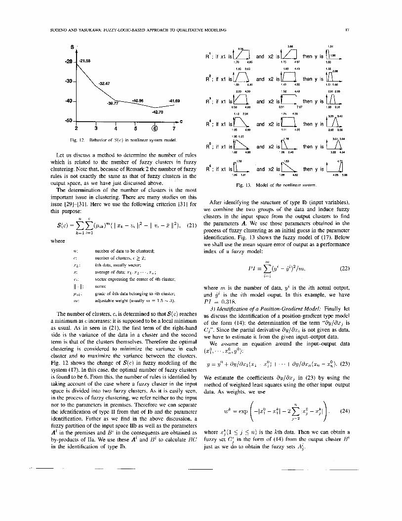
The number of clusters, c, is determined so that S( e ) reaches a minimum as c increases: it is supposed to be a local minimum as usual. As in seen in (21), the first term of the right-hand side is the variance of the data in a cluster and the second term is that of the clusters themselves. Therefore the optimal clustering is considered to minimize the variance in each cluster and to maximize the variance between the clusters. Fig. 12 shows the change of S ( c ) in fuzzy modeling of the system (17). In this case, the optimal number of fuzzy clusters is found to be 6. From this, the number of rules is identified by taking account of the case where a fuzzy cluster in the input space is divided into two fuzzy clusters. As it is easily seen, in the process of fuzzy clustering, we refer neither to the input nor to the parameters in premises. Therefore we can separate the identification of type I1 from that of Ib and the parameter identification. Futher as we find in the above discussion, a fuzzy partition of the input space IIb as well as the parameters Ai in the premises and Bi in the consequents are obtained as by-products of IIa. We use these A” and Bi to calculate RC in the identification of type Ib.

3.91 3.94 1.35 1.65

R5; if XI isw and x2 i s c then y is 1.02 4.98 1.06 2.40 3.22 4.94

R‘; if x l i s f i l l a and x2 i s K then y is a 1.05 1.81 1.06 4.62 4.05 5.06

Fig. 13. Model of the nonlinear sustem.

After identifying the structure of type Ib (input variables), we combine the two groups of the data and induce fuzzy clusters in the input space from the output clusters to find the parameters A. We use those parameters obtained in the process of fuzzy clustering as an initial guess in the parameter identification. Fig. 13 shows the fuzzy model of (17). Below we shall use the mean square error of output as a performance index of a fuzzy model:

where m is the number of data, yz is the ith actual output, and is the ith model ouput. In this example, we have PI = 0.318.

3) Identi’cation of a Position-Gradient Model: Finally let us discuss the identification of a position-gradient type model of the form (14): the determination of the term “dyldz, is Cj”. Since the partial derivative dy/dzi is not given as data, we have to estimate it from the given input-output data.

We assume an equation around the input-output data (z?. . . ’ . x;L, yo):

y = yo + dy/dzl(zl - z:) + . . . + dy/dz,(z,, - x:). (23)

We estimate the coefficients dy/dzj in (23) by using the method of weighted least squares using the other input-output data. As weights, we use

where .c;(l 5 , j 5 n ) is the kth data. Then we can obtain a fuzzy set Ci in the form of (14) from the output cluster Bz just as we do to obtain the fuzzy sets A i .


I Find the Darameters 6 I t

Divide data into two groups 1

Assume single variable among input candidates

i Find the parameters A with respect to each I group of data

P l P2 P3 P4

Fig. 15. Trapezoidal fuzzy set.

Calculate RC for each input variable

I

t

Combine two groups of data to reform the parameters A

I Estimate by/bx and find the parameters C for a position- I oradient tvDe model +

I Make parameters identification I

Fig. 14. Algorithm for identification. Fig. 16. Constraint for adjusting parameter

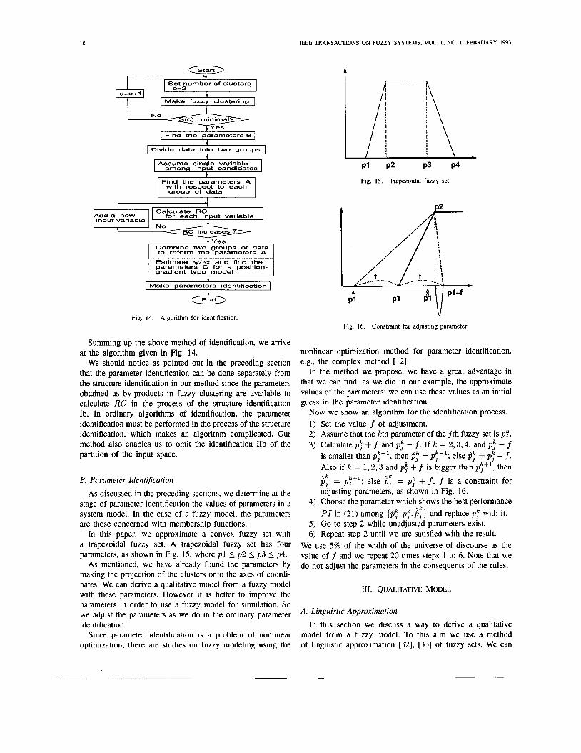
Summing up the above method of identification, we arrive at the algorithm given in Fig. 14.

We should notice as pointed out in the preceding section that the parameter identification can be done separately from the structure identification in our method since the parameters obtained as by-products in fuzzy clustering are available to calculate RC in the process of the structure identification Ib. In ordinary algorithms of identification, the parameter identification must be performed in the process of the structure identification, which makes an algorithm complicated. Our method also enables us to omit the identification IIb of the partition of the input space.

B. Parameter Ident$cation

As discussed in the preceding sections, we determine at the stage of parameter identification the values of parameters in a system model. In the case of a fuzzy model, the parameters are those concerned with membership functions.

In this paper, we approximate a convex fuzzy set with a trapezoidal fuzzy set. A trapezoidal fuzzy set has four parameters, as shown in Fig. 15, where p l 5 p 2 5 p3 5 p4.

As mentioned, we have already found the parameters by making the projection of the clusters onto the axes of coordinates. We can derive a qualitative model from a fuzzy model with these parameters. However it is better to improve the parameters in order to use a fuzzy model for simulation. So we adjust the parameters as we do in the ordinary parameter identification.

Since parameter identification is a problem of nonlinear optimization, there are studies on fuzzy modeling using the

nonlinear optimization method for parameter identification, e.g., the complex method [12].

In the method we propose, we have a great advantage in that we can find, as we did in our example, the approximate values of the parameters; we can use these values as an initial guess in the parameter identification.

Now we show an algorithm for the identification process. Set the value f of adjustment. Assume that the lcth parameter of the j th fuzzy set is pj". Calculate pj" + f and p: - f . If lc = 2,3 ,4 , and pj" - f is smaller than p$-', then 6; = $'; else 6: = pj" - f . Also if lc = 1 , 2 , 3 and p: + f is bigger than pS+l, then

p j = p;+l; else fij = pj" + f . f is a constraint for adjusting parameters, as shown in Fig. 16. Choose the parameter which shows the best performance PI in (21) among {fi:,p;,fij} and replace pj" with it. Go to step 2 while unadjusted parameters exist. Repeat step 2 until we are satisfied with the result.

- I C

- I C

We use 5% of the width of the universe of discourse as the value of f and we repeat 20 times steps 1 to 6. Note that we do not adjust the parameters in the consequents of the rules.

111. QUALITATIVE MODEL

A. Linguistic Approximation

In this section we discuss a way to derive a qualitative model from a fuzzy model. To this aim we use a method of linguistic approximation [32], [33] of fuzzy sets. We can


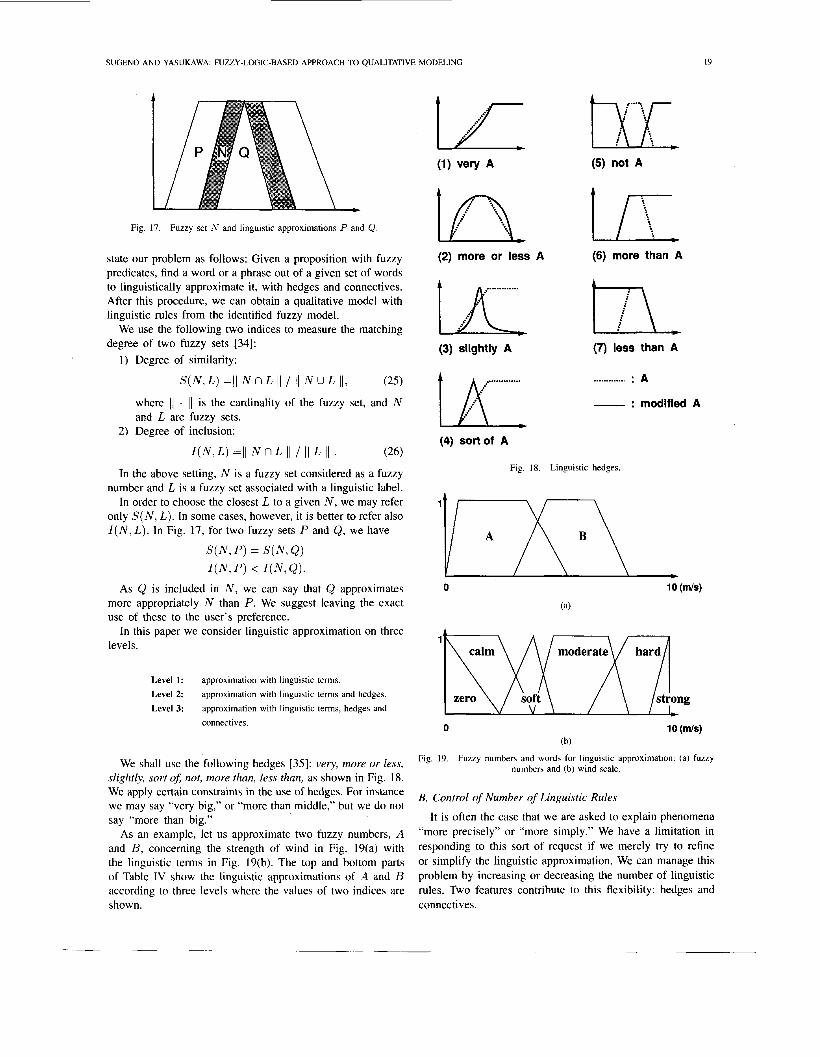
Fig. 17. Fuzzy set and linguistic approximations P and &.

state our problem as follows: Given a proposition with fuzzy predicates, find a word or a phrase out of a given set of words to linguistically approximate it, with hedges and connectives. After this procedure, we can obtain a qualitative model with linguistic rules from the identified fuzzy model.

We use the following two indices to measure the matching degree of two fuzzy sets [34]:

Degree of similarity:

S ( N , L ) =II N n L II / II N U L II, (25)

where ( 1 . 1 1 is the cardinality of the fuzzy set, and N and L are fuzzy sets. Degree of inclusion:

I ( N , L ) =II N n L II / II L II . (26)

the above setting, N is a fuzzy set considered as a fuzzy number and L is a fuzzy set associated with a linguistic label.

In order to choose the closest L to a given N , we may refer only S ( N , L ) . In some cases, however, it is better to refer also I ( N , L ) . In Fig. 17, for two fuzzy sets P and Q, we have

S ( N , P ) = S ( N , Q) W , p ) < I ( N , Q ) .

As Q is included in N , we can say that Q approximates more appropriately N than P. We suggest leaving the exact use of these to the user’s preference.

In this paper we consider linguistic approximation on three levels.

Level 1: Level 2: Level 3:

approximation with linguistic terms. approximation with linguistic terms and hedges. approximation with linguistic terms, hedges and connectives.

We shall use the following hedges [35]: very, more or less, slightly, sort oj not, more than, less than, as shown in Fig. 18. We apply certain constraints in the use of hedges. For instance we may say “very big,” or “more than middle,” but we do not say “more than big.”

As an example, let us approximate two fuzzy numbers, A and B, concerning the strength of wind in Fig. 19(a) with the linguistic terms in Fig. 19(b). The top and bottom parts of Table IV show the linguistic approximations of A and B according to three levels where the values of two indices are shown.

(2) more or less A (6) more than A l)f- ............. I-\* f

2‘

(3) slightly A (7) less than A

.. ............ ............. : A

- : modified A

(4) sort of A

Fig. 18. Linguistic hedges.

0

0 1 0 (mk) (b)

numbers and (b) wind scale. Fig. 19. Fuzzy numbers and words for linguistic approximation: (a) fuzzy

B. Control of Number of Linguistic Rules

It is often the case that we are asked to explain phenomena “more precisely” or “more simply.” We have a limitation in responding to this sort of request if we merely try to refine or simplify the linguistic approximation. We can manage this problem by increasing or decreasing the number of linguistic rules. Two features contribute to this flexibility: hedges and connectives.

20 IEEE TRANSACTIONS ON FUZZY SYSTEMS, VOL. 1 , NO. 1, FEBRUARY 1993

TABLE IV RESULTS OF LINGUISTIC APPROXIMATION

Level Linguistic Expression S I ~~

1 calm 0.62 0.96

2 less than soft 0.87 0.97

3 more or less calm or more or 0.94 0.94 less soft

Level Linguistic Expression S I

I moderate , 0.76 0.92

2 more or less moderate 0.81 0.83

3 not strong but more or less 0.86 0.98 moderate

As we adopt a fuzzy clustering method for the identification of IIa i.e., the number of rules, we can simply control the number of linguistic rules by adjusting the number of fuzzy clusters. This is also a great advantage of the proposed method.

IV. ILLUSTRATIVE EXAMPLES We deal with six illustrative examples in this section. The

first example involves qualitative modeling of a nonlinear system, which has been partly discussed in the previous section. The second is also a numerical example in which we discuss the performance of our fuzzy modeling method. In the third example we make a qualitative model of a dynamical process. The fourth and fifth examples are concerned with qualitative modeling of human operation at process control. In the final example we make a qualitative model to explain the trend in the time series data of the price of a stock.

In order to understand the examples in connection with the preceding discussions, let us list the key points:

a) fuzzy model of position type, b) fuzzy model of position-gradient type, c) qualitative model, d) structure of type Ib: input variables, e) control of the number of linguistic rules, f) structure of type IIa: number of rules, g) parameter identification. In what follows, we shall attach symbols (a)-(e) to each

example. Throughout the examples, (f), the structure identification of type IIa, and (g), the parameter identification, are performed.

A. Nonlinear System (a , b, c, d )

This example deals with the explanation of the proposed method of identification. Let us recall a static and nonlinear two input-single output system of the type shown in (17):

This system shows the nonlinear characteristic illustrated in Fig. 5 and we use the data in Table 11. The process of the identification of type IIa has been shown in Table 111 and we have found the true inputs .c1 and .r2. The optimal number of

2.10

1.30

R'; if x i ism and x2 i s m then y is 1.15 4.97 1.06 4.85

1.84 3.45 1.93 3.20

R'; if x i i s t n and x2 ism- then y is r- 1.46 4.06 1.16 3.79 1.51 2.60

I 4 n D e l 2.02 2.51 2.65 . . .-

R3; if XI i s k and x2 i s h then y is 1.10 2.76 1.63 5.21 1.W 3.31

3.35 3.42 2.00 227 1.24 2.92

R4 ; if XI i s k and x2 is&, then y is 2.08 2.32 124 3.60 2.88 3.98

3.91 3.94

R5; if XI is& and x2 i s K then y is t/l 1.40 5.95 1.03 2.88 3.22 4.94

Re; if x i i s f i , and x2 is& then y is 1.m 2.57 1.06 4.93 4.05 5.m

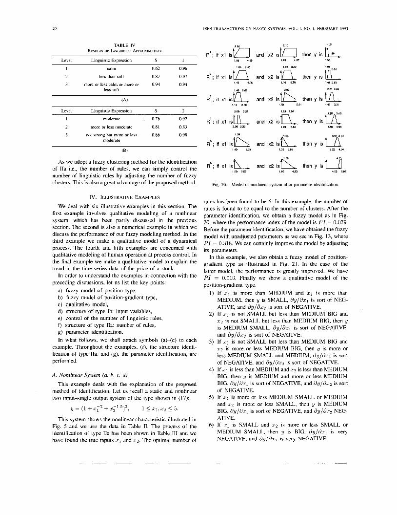
Fig. 20. Model of nonlinear system after parameter identification.

rules has been found to be 6. In this example, the number of rules is found to be equal to the number of clusters. After the parameter identification, we obtain a fuzzy model as in Fig. 20, where the performance index of the model is P I = 0.079. Before the parameter identification, we have obtained the fuzzy model with unadjusted parameters as we see in Fig. 13, where PI = 0.318. We can certainly improve the model by adjusting its parameters.

In this example, we also obtain a fuzzy model of position- gradient type as illustrated in Fig. 21. In the case of the latter model, the performance is greatly improved. We have PI = 0.010. Finally we show a qualitative model of the position-gradient type.

I ) If z1 is more than MEDIUM and 2 2 is more than MEDIUM, then y is SMALL, .3y/dzl is sort of NEG- ATIVE, and dy/da2 is sort of NEGATIVE.

2 ) If 2 1 is not SMALL but less than MEDIUM BIG and 2 2 is not SMALL but less than MEDIUM BIG, then y is MEDIUM SMALL, dy/dzl is sort of NEGATIVE, and dy/dz2 is sort of NEGATIVE.

3) If 2 1 is not SMALL but less than MEDIUM BIG and :cp is more or less MEDIUM BIG, then y is more or less MEDIUM SMALL and MEDIUM, dy/d:1;1 is sort of NEGATIVE, and i)y/d:~2 is sort of NEGATIVE.

4) If 21 is less than MEDIUM and 1c2 is less than MEDIUM BIG, then y is MEDIUM and more or less MEDIUM BIG, i)y/d:cl is sort of NEGATIVE, and i)y/dzp is sort of NEGATIVE.

5) If :~ '1 is more or less MEDIUM SMALL or MEDIUM and 2 2 is more or less SMALL, then y is MEDIUM BIG, i)y/i)zl is sort of NEGATIVE, and dy/i):c2 NEG- ATIVE.

6) If :c1 is SMALL and x 2 is more or less SMALL or MEDIUM SMALL, then y is BIG, dy/i)zl is very NEGATIVE, and dy/d:1;2 is very NEGATIVE.


~

21

* Consequents are singletons

Fig. 21. Position-gradient model of nonlinear system.

x2

1 xl 0 3 4 6 7 10

Fig. 22. Fuzzy system.

We can understand the performance of the model by referring to the characteristics of the system shown in Fig. 5.

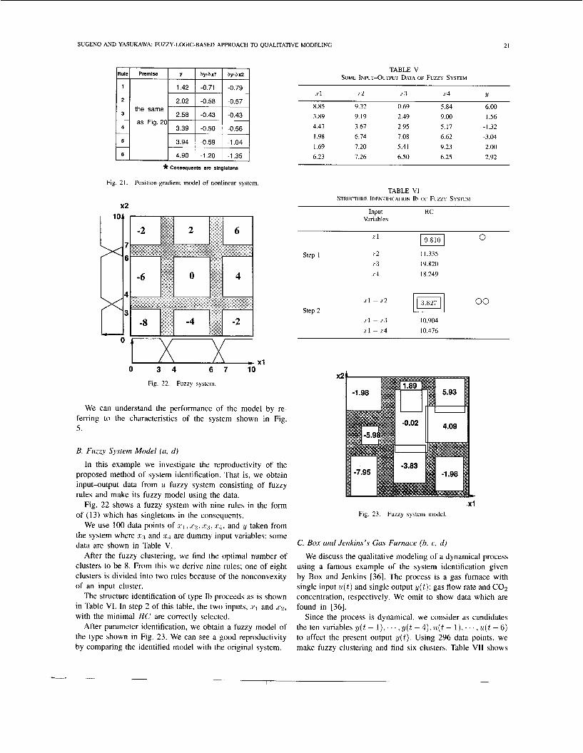
B. Fuzzy System Model (a, d )

In this example we investigate the reproductivity of the proposed method of system identification. That is, we obtain input4utput data from a fuzzy system consisting of fuzzy rules and make its fuzzy model using the data.

Fig. 22 shows a fuzzy system with nine rules in the form of (13) which has singletons in the consequents.

We use 100 data points of XI . 2 2 . : X S , :CA, and y taken from the system where 2 3 and :CA are dummy input variables; some data are shown in Table V.

After the fuzzy clustering, we find the optimal number of clusters to be 8. From this we derive nine rules; one of eight clusters is divided into two rules because of the nonconvexity of an input cluster.

The structure identification of type Ib proceeds as is shown in Table VI. In step 2 of this table, the two inputs, :1:1 and 2 2 ,

with the minimal RC are correctly selected. After parameter identification, we obtain a fuzzy model of

the type shown in Fig. 23. We can see a good reproductivity by comparing the identified model with the original system.

TABLE V SOME INPUT-OUTPUT DATA OF FUZZY SYSTEM

.1' 1 1' 2 1' 3 1' 1 Y ~~ ~

8.85 9.32 0.69 5.84 6.00 3.89 9.19 2.49 9.00 1.56 4.43 3.67 2.95 5.17 -1.32 1.98 6.74 7.08 6.62 -3.04 1.69 7.20 5.41 9.23 -2.00 6.23 7.26 6.50 6.25 2.92

TABLE VI STRUCTURE IDENTIFICATION Ib OF Fuzzy SYSTEM

Input RC Variables

.1' 1

Step 1 .r2 .2.3

.rl

0

1 1.335 19.820 18.249

.rl - .r2

Step 2 .r1 - .r3 .2.1 - .1'1

10.904 10.476

.xl Fig. 23. Fuzzy system model.

C. Box and Jenkins's Gas Furnace (b, c, d )

We discuss the qualitative modeling of a dynamical process using a famous example of the system identification given by Box and Jenkins [36]. The process is a gas furnace with single input u ( t ) and single output y(t): gas flow rate and CO2 concentration, re5pectively. We omit to show data which are found in [36].

Since the process is dynamical, we consider as candidates the ten variables y ( t - 1). . . . , g ( t - 4). u(t - 1). . . . . u( t - 6) to affect the present output y(t). Using 296 data points, we make fuzzy clustering and find six clusters. Table VI1 shows

22

R'

IEEE TRANSACTIONS ON FUZZY SYSTEMS, VOL. I , NO. 1, FEBRUARY 1993

47.66 0.79 -2.36 -1.39 38.51 55.16 0.01 1.4 -3.51 13.59

TABLE VI1 STRUCTURE IDENTIFICATION Ib OF GAS FURNACE

Input RC Variables

m 0

Step 1

Y ( t - 1)

Y(t - 2 ) Y(t - 3)

Y(t - 4) u( t - 1) u ( t - 2 ) u ( t - 3)

u ( t - 4 )

u( t - 5 )

u ( t - 6)

Y(t - 1) - Y ( t - 2 ) ?At - 1) - Y(t - 3 )

Y(t - 1) - Y ( t - 4) g ( t - 1) - u ( t - 1)

y ( t - 1) - u ( t - 2 )

Y ( t - 1) - u ( t - 3 )

g ( t - 1) - u ( t - 4)

y(t - 1 ) - u ( t - 5) Y ( t - 1) - u ( t - 5 )

g ( t -1)- u ( t -4)- u ( t -1) Y ( t - 1 ) - u ( t - 4 ) - u ( t - 2 )

Step 2

step 3 y ( t - l ) - - ( t - 4 ) - u ( t - 3 )

y(t - 1 ) - u ( f - 4 ) - u ( t - 5 )

g ( t - 1 ) - u ( t - 4 ) - ~ ( f - 6 )

U

2.276 4.151

5.720

6.724

4.816

3.257

1.869 1.465

2.040

0.973

1.067 1.020 0.745

0.598

0.439

X

X

X

0.565

0.846

0.439 X

0.429 X

0.454 X

0.499 X

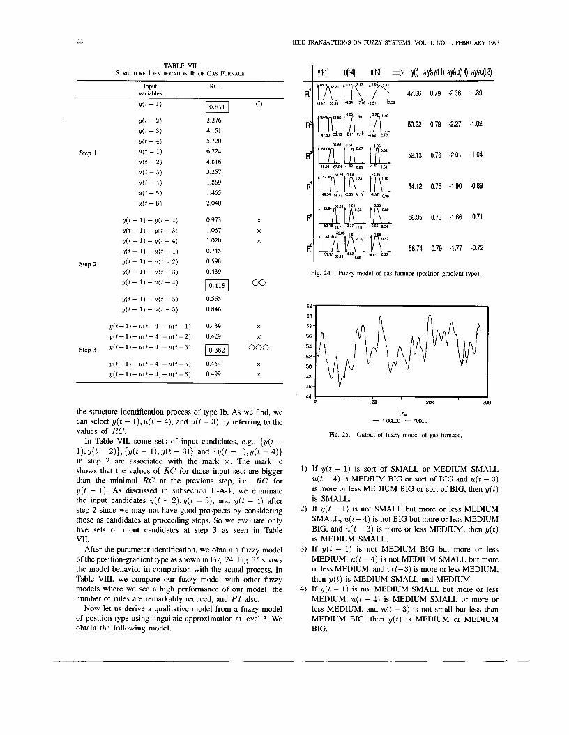
the structure identification process of type Ib. As we find, we can select y(t - l), u(t - 4), and u(t - 3) by referring to the values of RC.

In Table VII, some sets of input candidates, e.g., {y(t -

in step 2 are associated with the mark x. The mark x shows that the values of RC for those input sets are bigger than the minimal RC at the previous step, i.e., RC for y(t - 1). As discussed in subsection 11-A-1, we eliminate the input candidates y(t - 2), y(t - 3) , and y(t - 4) after step 2 since we may not have good prospects by considering those as candidates at proceeding steps. So we evaluate only five sets of input candidates at step 3 as seen in Table VII.

After the parameter identification, we obtain a fuzzy model of the position-gradient type as shown in Fig. 24. Fig. 25 shows the model behavior in comparison with the actual process. In Table VIII, we compare our fuzzy model with other fuzzy models where we see a high performance of our model; the number of rules are remarkably reduced, and P I also.

Now let us derive a qualitative model from a fuzzy model of position type using linguistic approximation at level 3. We obtain the following model.

11, Y ( t - 211, {Y( t - I), Y ( t - 3)) and { d t - 11, Y( t - 4))

I y(t-1) u(t-4) u(t-3) 3 y(t) ayby(t-1) ayhu(t-4) ay/w(t-3)

R( rr;1°1.3: lJ1.: 50.22 0.79 -2.27 -1.02

47.50 55.10 -2.61 2.1 -292 2.79

58.74 0.79 -1.77 -0.72 51.11 63,13 4.62 4.41 286

1 .m

Fig. 24. Fuzzy model of gas furnace (position-gradient type).

I I

T I E - PROCESS '.... MODEL

Fig. 25. Output of fuzzy model of gas furnace.

1) If y ( t - 1) is sort of SMALL or MEDIUM SMALL u(t - 4) is MEDIUM BIG or sort of BIG and u(t - 3) is more or less MEDIUM BIG or sort of BIG, then y(t) is SMALL.

2) If y(t - 1) is not SMALL but more or less MEDIUM SMALL, u(t - 4) is not BIG but more or less MEDIUM BIG, and u(t - 3) is more or less MEDIUM, then y(t) is MEDIUM SMALL.

3) If y(t - 1) is not MEDIUM BIG but more or less MEDIUM, u(t - 4) is not MEDIUM SMALL but more or less MEDIUM, and u(t-3) is more or less MEDIUM, then y(t) is MEDIUM SMALL and MEDIUM.

4) If y(t - 1) is not MEDIUM SMALL but more or less MEDIUM, u(t - 4) is MEDIUM SMALL or more or less MEDIUM, and u(t - 3 ) is not small but less than MEDIUM BIG, then y( t ) is MEDIUM or MEDIUM BIG.

23 SUGENO AND YASUKAWA: FUZZY-LOGIC-BASED APPROACH TO QUALITATIVE MODELING

TABLE VI11 COMPARISON OF FUZZY MODEL WITH OTHER MODELS

(Candidates of input variables )

Model Name Inputs Number Model of Error

Rules Tong’s model

[51 19 0.469

Y ( t - 1 ). 81 0.320 Pedryc’s model [6] tr(t - 4 )

Xu’s model ~ 7 1

25 0.328

- 0.193

r/(t - 11, Y ( t - 21, Y ( t - 31, 2 0.068 model [35] u( t - l ) , n(t - 2 ) , l / ( t - 3 )

Takagi Sugeno

Position- Y ( t -

model t t ( t - 3 ) gradient u ( t - 4), 6 0.190

5) If y(t - 1) is not BIG but more or less MEDIUM BIG, U ( t - 4) is MEDIUM SMALL or MEDIUM, and U ( t - 3 ) is not SMALL but more or less MEDIUM SMALL, then y ( t ) is MEDIUM BIG and sort of BIG.

6) If y(t-1) is MEDIUM BIG or more or less BIG, u(t-4) is more or less MEDIUM SMALL or MEDIUM, and u(t - 3 ) is less than MEDIUM, then y(t) is very BIG.

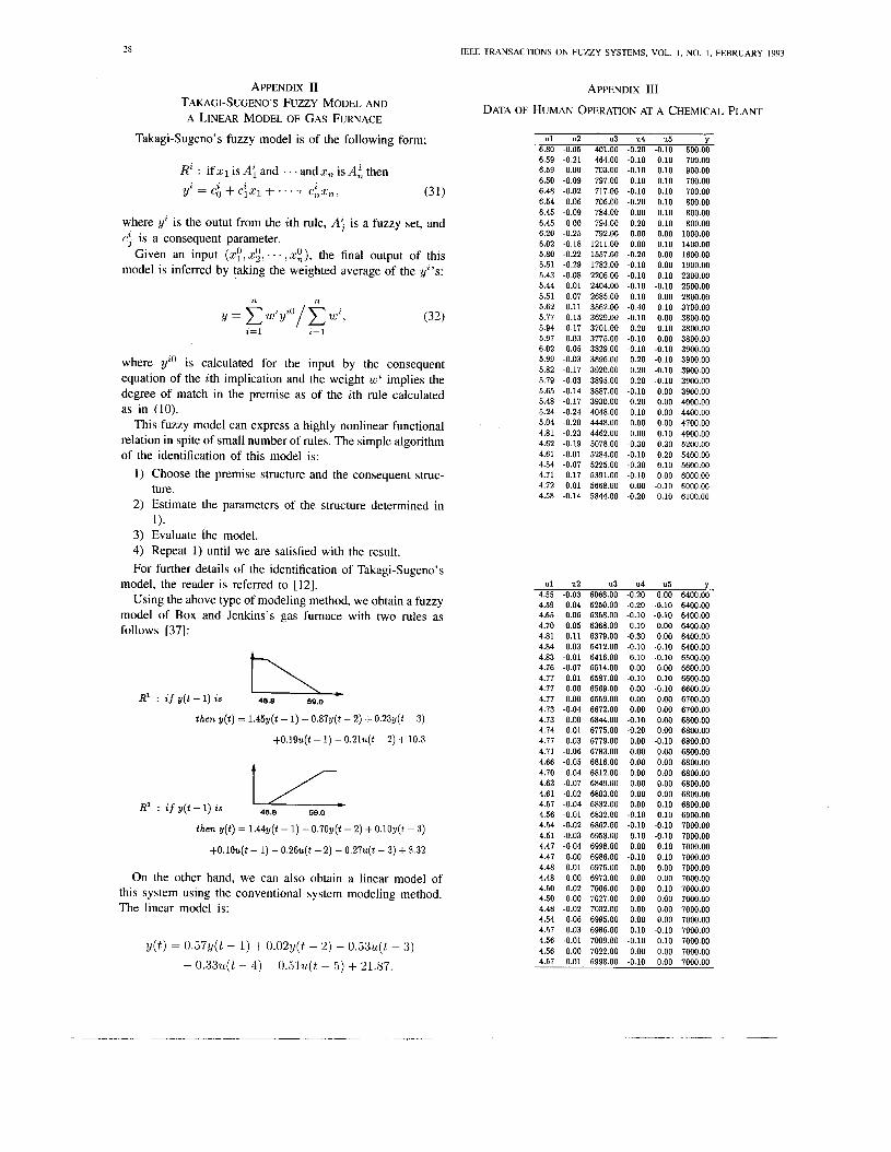
As is well known, we can make a linear model of this process. The performance index of the identified linear model is P I = 0.193. The P170.190, of our fuzzy model is almost the same as that of the linear model. We should remark that we do not aim at a good numerical model by fuzzy modeling in this study. If we want to do it by fuzzy modeling, we can use Takagi-Sugeno’s fuzzy model and we can improve the performance quite a bit more such that P I = 0.068 Wl.

We will show this fuzzy model as well as a linear model in Appendix 11.

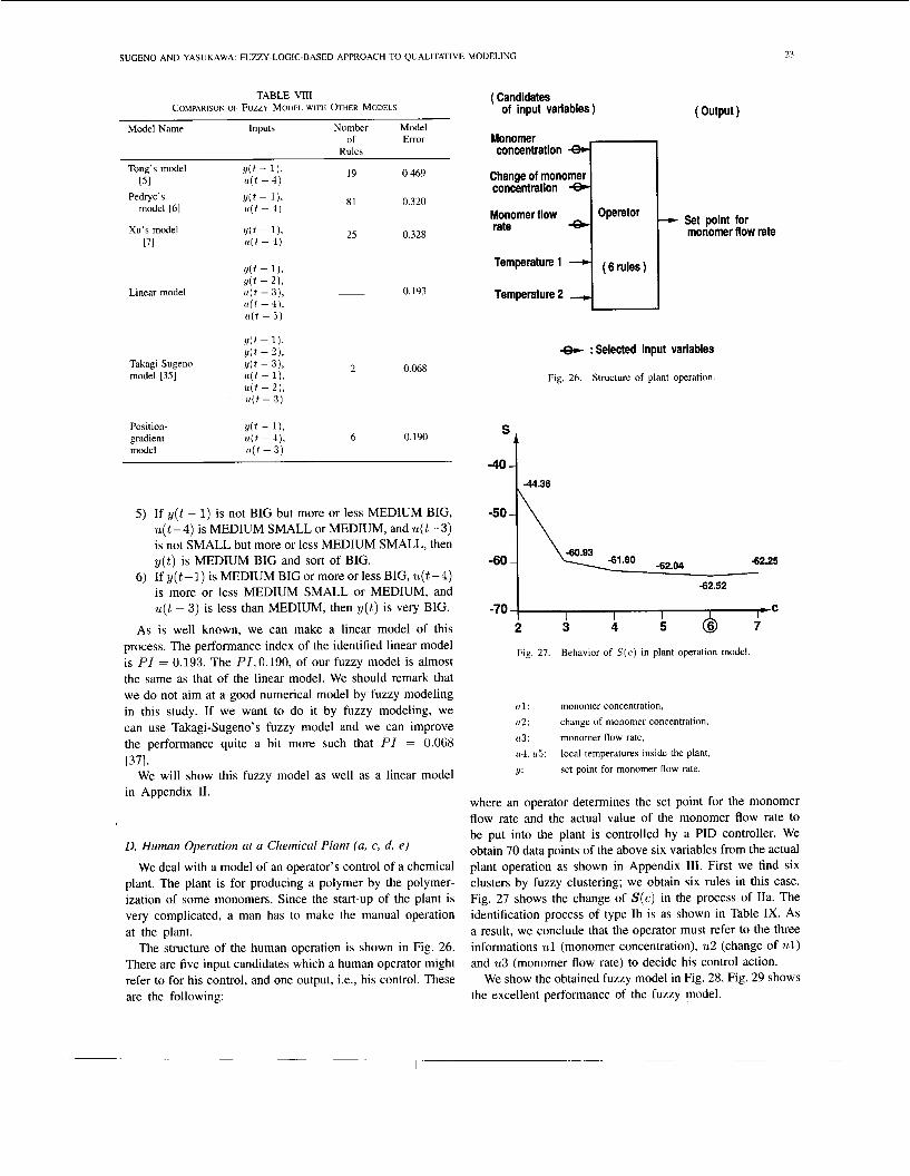
D. Human Operation ut a Chemical Plant ( U , c, d, e )

We deal with a model of an operator’s control of a chemical plant. The plant is for producing a polymer by the polymer- ization of some monomers. Since the start-up of the plant is very complicated, a man has to make the manual operation at the plant.

The structure of the human operation is shown in Fig. 26. There are five input candidates which a human operator might refer to for his control, and one output, i.e., his control. These are the following:

( output )

Monomer concentration

Change of monomer concentration

Set point for monomer flow rate

Monomer flow rate

( 6 rules) I U Temperature 2

8, : Selected input variables

Fig. 26. Structure of plant operation

t

-50 K -62.52 I

-70 I Y C 3 I 4 b b 7 I

2

Fig. 27. Behavior of S ( c ) in plant operation model.

c t l : monomer concentration, t t 2 : change of monomer concentration, 113: monomer flow rate, 114. tt.5: local temperatures inside the plant,

Y: set point for monomer flow rate.

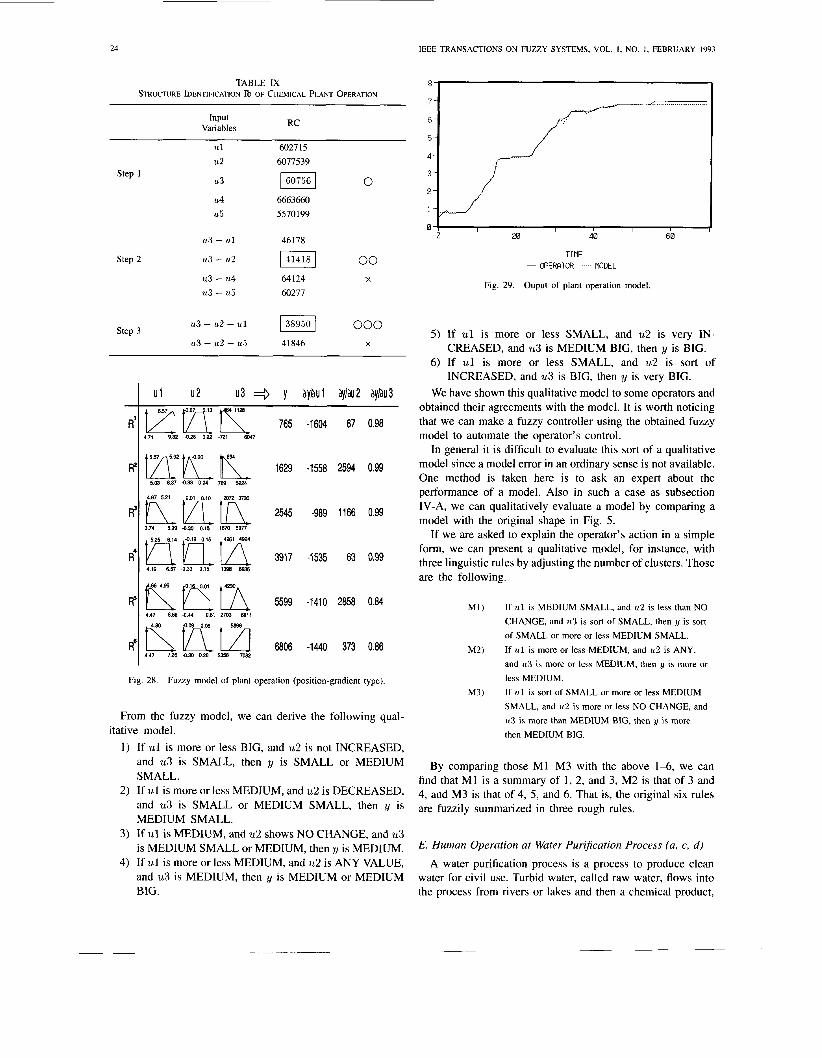
where an operator determines the set point for the monomer flow rate and the actual value of the monomer flow rate to be put into the plant is controlled by a PID controller. We obtain 70 data points of the above six variables from the actual plant operation as shown in Appendix 111. First we find six clusters by fuzzy clustering; we obtain six rules in this case. Fig. 27 shows the change of S ( c ) in the process of IIa. The identification process of type Ib is as shown in Table IX. As a result, we conclude that the operator must refer to the three informations u l (monomer concentration), u2 (change of u l ) and 213 (monomer flow rate) to decide his control action.

We show the obtained fuzzy model in Fig. 28. Fig. 29 shows the excellent performance of the fuzzy model.

24

~

R“

R6

TABLE 1X STRUCTURE IDENTIFICATION Ib OF CHEMICAL PLANT OPERATION

1 5 7 ; 9 2 5.03 6.37 4.38 0.M 769 5224

4.97 5.21 4.01 0.10 2072 3730 aurn 3.74 6.09 4.30 0.15 16m 5977

d!lntn 4.16 6.57 4.33 0.15 1398 6636

F- ,42h 4.47 K E D 726 4.30 0.20 2358 7032

5.25 6.14 4.19 0.15 4261 4924

4.47 6.66 4.44 0.61 2703 €011

IEEE TRANSACTIONS ON FUZZY SYSTEMS, VOL. I , NO. 1 , FEBRUARY 1993

RC Input Variables

U 1 6027 15 U2 6077539

U 3

U 4 6663660 U 5 5570 199

lGOTjGI 0 Step I

Step 2

U3 - U 1 46178

U 3 - U 2 00 U3 - U4 64124 X

U3 - U 5 60277

U 3 - U 2 - U 1 138950 I 000 Step 3 U 3 - U 2 - U 5 41846 X

I U1 U 2 U3 =) y a y b u l yaU2 aylau3

R’ 4.71 9.32 4.28 0.22 -721 6047

765 -1604 67 0.98

1629 -1558 2594 0.99

2545 -989 1166 0.99

3917 -1535 63 0.99

5599 -1410 2858 0.84

6806 -1440 373 0.86

Fig. 28. Fuzzy model of plant operation (position-gradient type).

From the fuzzy model, we can derive the following qual-

1) If ul is more or less BIG, and u2 is not INCREASED, and u3 is SMALL, then y is SMALL or MEDIUM SMALL.

2 ) If u1 is more or less MEDIUM, and u2 is DECREASED, and u3 is SMALL or MEDIUM SMALL, then y is MEDIUM SMALL.

3 ) If ul is MEDIUM, and u2 shows NO CHANGE, and u3 is MEDIUM SMALL or MEDIUM, then y is MEDIUM.

4) If u1 is more or less MEDIUM, and u2 is ANY VALUE, and u3 is MEDIUM, then y is MEDIUM or MEDIUM BIG.

itative model.

I I I I I 0 20 40 60

TIRE - OPERATOR MODEL

Ouput of plant operation model. Fig. 29.

5 ) If ul is more or less SMALL, and u2 is very IN- CREASED, and u3 is MEDIUM BIG, then y is BIG.

6) If ul is more or less SMALL, and u2 is sort of INCREASED, and u3 is BIG, then y is very BIG.

We have shown this qualitative model to some operators and obtained their agreements with the model. It is worth noticing that we can make a fuzzy controller using the obtained fuzzy model to automate the operator’s control.

In general it is difficult to evaluate this sort of a qualitative model since a model error in an ordinary sense is not available. One method is taken here is to ask an expert about the performance of a model. Also in such a case as subsection IV-A, we can qualitatively evaluate a model by comparing a model with the original shape in Fig. 5.

If we are asked to explain the operator’s action in a simple form, we can present a qualitative model, for instance, with three linguistic rules by adjusting the number of clusters. Those are the following.

M I ) If u l is MEDIUM SMALL, and rr2 is less than NO CHANGE, and (13 is sort of SMALL, then y is sort of SMALL or more or less MEDIUM SMALL. If ul is more or less MEDIUM, and u2 is ANY, and i t3 is more or less MEDIUM, then y is more or less MEDIUM. If u l is sort of SMALL or more or less MEDIUM SMALL, and tr2 is more or less NO CHANGE, and I13 is more than MEDIUM BIG, then y is more then MEDIUM BIG.

M2)

M3)

By comparing those MlLM3 with the above 1-6, we can find that M 1 is a summary of 1, 2, and 3, M2 is that of 3 and 4, and M3 is that of 4, 5, and 6. That is, the original six rules are fuzzily summarized in three rough rules.

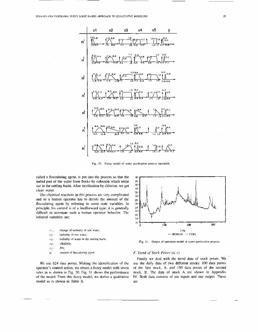
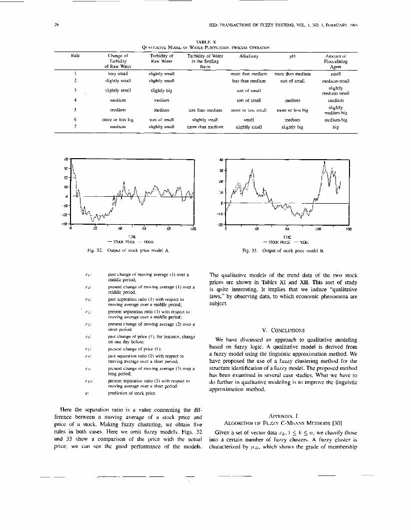
E. Human Operation ut Water Purification Process (a, e, d )

A water purification process is a process to produce clean water for civil use. Turbid water, called raw water, flows into the process from rivers or lakes and then a chemical product,


R'

2 R

R3

Ft

Fl

6 R

7 R

X I x2 x3 x4 x5 Y

0.W 30.14

7 .11 7 .21 28.99 14.76 15.91 171.68 256.11

Fig. 30. Fuzzy model of water purification process operation.

called a floccul ting agent, is put into the process so that the turbid part of the water form flocks by cohesion which settle out in the settling basin. After sterilization by chlorine, we get clean water.

The chemical reactions in this process are very complicated and so a human operator has to decide the amount of the flocculating agent by referring to some state variables. In principle, his control is of a feedforward type; it is generally difficult to automate such a human operator behavior. The referred variables are:

X I :

~ 2 : turbidity of raw water, . I , : $ :

. r . ~ : alkalinity,

.r:: PH,

change of turbidity of raw water,

turbidity of water in the settling basin,

CJ: amount of flocculating agent.

We use 624 data points. Making the identification of the operator's control action, we obtain a fuzzy model with seven rules as is shown in Fig. 30. Fig. 31 shows the performance of the model. From this fuzzy model, we derive a qualitative model as is shown in Table X.

TIRE - OPERATOR MODEL

Fig. 3 1. Output of operation model at water purification process.

F. Trend of Stock Prices ( U , c)

Finally we deal with the trend data of stock prices. We use the daily data of two different stocks: 100 data points of the first stock, A, and 150 data points of the second stock, B. The data of stock A are shown in Appendix IV. Both data consists of ten inputs and one output. These are

26 IEEE TRANSACTIONS ON FUZZY SYSTEMS, VOL. 1, NO. I , FEBRUARY 1993

TABLE X QUALITATIVE MODEL OF WATER PURIFICATION PRWESS OPERATION

Rule Change of Turbidity of Turbidity of Water Alkalinity P” Amount of Turbidity Raw Water in the Settling Flocculating

of Raw Water Basin Agent 1 very small slightly small more than medium more than medium small 2 slightly small slightly small less than medium sort of small medium-small

s I i g h t I y medium-small 3 slightly small slightly big sort of small

4 medium medium sort of small medium medium slightly

medium-big 5 medium medium less than medium more or less small more or less big

6 more or less big sort of small slightly small small medium medium-big 7 medium slightly small more than medium slightly small slightly big big

-30 , I I

0 I I I l l

20 40 60 80 1EZl

TIME - STDCK PRICE ..... EODEL

Fig. 32. Output of stock price model A.

past change of moving average ( I ) over a middle period; present change of moving average ( I ) over a middle period; past separation ratio ( I ) with respect to moving average over a middle period; present separation ratio ( I ) with respect to moving average over a middle period; present change of moving average (2) over a short period; past change of price ( I ) , for instance, change on one day before; present change of price ( I ) : past separation ratio (2) with respect to moving average over a short period; present change of moving average (3) over a long period; present separation ratio (3) with respect to moving average over a short period; prediction of stock price.

Here the separation ratio is a value concerning the difference between a moving average of a stock price and price of a stock. Making fuzzy clustering, we obtain five rules in both cases. Here we omit fuzzy models. Figs. 32 and 33 show a comparison of the price with the actual price; we can see the good performance of the models.

-20 1 I I I I

0 40 80 120 160

TIUE - STOCK PRICE ..... MODEL

Output of stock price model B. Fig. 33.

The qualitative models of the trend data of the two stock prices are shown in Tables XI and XII. This sort of study is quite interesting. It implies that we induce “qualitative laws,” by observing data, to which economic phenomena are subject.

V. CONCLUSIONS We have discussed an approach to qualitative modeling

based on fuzzy logic. A qualitative model is derived from a fuzzy model using the linguistic approximation method. We have proposed the use of a fuzzy clustering method for the structure identification of a fuzzy model. The proposed method has been examined in several case studies. What we have to do further in qualitative modeling is to improve the linguistic approximation method.

APPENDIX I ALGORITHM OF FUZZY C-MEANS METHODS [30]

Given a set of vector data Z k , 1 5 k 5 ri, we classify those into a certain number of fuzzy clusters. A fuzzy cluster is characterized by p,k. which shows the grade of membership


TABLE XI QUALITATIVE MODEL OF TREND OF STOCK PRICE A

Change of Moving Separation Ratio I Change Change of Price 1 Separation Change Separation Average 1 of Ratio 2 of Ratio 3

Rule Moving Average

Moving Average Prediction

7

Past Now Past Now Now Past Now level

level

more or less level

more or less level

level or rise

Now more less rise

more or sort of less zero rise

more or level less zero

more or sort of less zero decline

more than decline

zero

zero

Now Past

1 more or less rise

2

3

level or rise

level or decline

level or decline

level

rise

sort of plus

more or less zero

plus

more than zero

less than zero

minus

sort of minus

more or less zero

plus

level

more or less level

more or less level

more or less level

sort of rise

level

level or rise

sort of rise

sort of rise

rise more or less zero


sort of more or decline less zero

Er::: 5 level or

rise


level sort of plus

TABLE XI1 QUALITATIVE MODEL OF TREND OF STOCK PRICE B

Change of Moving Separation Ratio 1 Change Change of Price 1 Separation Change Separation Average 1 of Ratio 2 of Ratio 3

Moving Moving Prediction Rule Average Average

2 3 Past Now Past Now Now Past Now Past Now Now

1 sort of level or less than sort of level sort of more or sort of sort of more or rise rise decline zero minus decline less level minus decline less zero

level or level or less than more or level or sort of sort of more than sort of rise decline zero less zero rise decline rise zero rise

3 level or level more or more or sort of level or sort of level rise less zero less zero rise rise rise

more or more or slightly more or level or more or level or less than sort of less rise less zero plus less level rise less zero decline zero decline 4

5 more or more or plus more level sort of level sort of more or decline less rise less rise than zero decline minus less zero

3) Calculate the element of a new U( ' ) as follows for of the kth data, xk, belonging to the ith cluster. We assume that 1 = 1 + 1 :

where c is the number of clusters, and we define a matrix U consisting of pik .

Our problem now is to find c and to determine U . The algorithm is as follows

1) Set c = 2, an initial value U(1) of U and 1 = 1. 2) Calculate the center wi of the fuzzy cluster by

n

4) If 1 1 U(l- l ) - U ( l ) I ( < - E , then stop; otherwise go to step

In this algorithm, r n is an adjustable parameter, which is 2.

set as 2 in this paper.

We define the distance from the kth data to the center of the ,ith cluster by

~

28 IEEE TRANSACTIONS ON FUZZY SYSTEMS, VOL. I . NO. I . FEBRUARY 1993

APPENDIX I1 TAKAGI-SUGENO’S FUZZY MODEL AND

A LINEAR MODEL OF GAS FURNACE

Takagi-Sugeno’s fuzzy model is of the following form;

Ri : if x1 is Ai and . . . and x, is AA then

yi = c6 + c;x1 + . . . + cix,, (31)

where yz is the outut from the ith rule, A; is a fuzzy set, and c; is a consequent parameter.

Given an input (xy , x:, . . . , x:), the final output of this model is inferred by taking the weighted average of the yz’s:

n n

where yio is calculated for the input by the consequent equation of the ith implication and the weight w2 implies the degree of match in the premise as of the ith rule calculated as in (10).

This fuzzy model can express a highly nonlinear functional relation in spite of small number of rules. The simple algorithm of the identification of this model is:

1 ) Choose the premise structure and the consequent struc-

2) Estimate the parameters of the structure determined in

3) Evaluate the model. 4) Repeat 1 ) until we are satisfied with the result. For further details of the identification of Takagi-Sugeno’s

model, the reader is referred to [12]. Using the above type of modeling method, we obtain a fuzzy

model of Box and Jenkins’s gas furnace with two rules as follows [37]:

ture.

1).

then y(t) = 1.45y(t - 1) - 0.87y(t - 2) + 0.23y(t - 3)

+0.19~(t - 1) - 0.214t - 2) + 10.3

48.8 59.0 Rz : i f ~ ( t - 1) is

then y(t) = 1.44y(t - 1) - 0.70y(t - 2) + O.lOy(t - 3)

+O.lOu(t - 1) - 0 . 2 6 ~ ( t - 2) - 0.27u(t - 3) + S.32

On the other hand, we can also obtain a linear model of this system using the conventional system modeling method. The linear model is:

y(t) = 0.57y(t - 1) + 0.02y(t - 2) - 0.53,/L(t - 3 )

- 0 . 3 3 * ~ ( t - 4) - 0 . 5 1 ~ ( t - 5) + 21.87.

APPENDIX I11 DATA OF HUMAN OPERATION AT A CHEMICAL PLANT

U1 U2 6.80 -0.05 6.59 -0.21 6.59 0.00 6.50 -0.09 6.48 -0.02 6.54 0.06 6.45 -0.09 6.45 0.00 6.20 -0.25 6.02 -0.18 5.80 -0.22 5.51 -0.29 5.43 -0.08 5.44 0.01 5.51 0.07 5.62 0.11 5.77 0.15 5.94 0.17 5.97 0.03 6.02 0.05 5.99 -0.03 5.82 -0.17 5.79 -0.03 5.65 -0.14 5.48 -0.17 5.24 -0.24 5.04 -0.20 4.81 -0.23 4.62 -0.19 4.61 -0.01 4.54 -0.07 4.71 0.17 4.72 0.01 4.58 -0.14

U1 U2 4.55 -0.03 4.59 0.04 4.65 0.06 4.70 0.05 4.81 0.11 4.84 0.03 4.83 -0.01 4.76 -0.07 4.77 0.01 4.77 0.00 4.77 0.00 4.73 -0.04 4.73 0.00 4.74 0.01 4.77 0.03 4.71 -0.06 4.66 -0.05 4.70 0.04 4.63 -0.07 4.61 -0.02 4.57 -0.04 4.56 -0.01 4.54 -0.02 4.51 -0.03 4.47 -0.04 4.47 0.00 4.48 0.01 4.48 0.00 4.50 0.02 4.50 0.00 4.48 -0.02 4.54 0.06 4.57 0.03 4.56 -0.01 4.56 0.00 4.57 0.01

U3 U4 U5 401.00 -0.20 -0.10 464.00 -0.10 0.10 703.00 -0.10 0.10 797.00 0.10 0.10 717.00 -0.10 0.10 706.00 -0.20 0.10 784.00 0.00 0.10 794.00 -0.20 0.10 792.00 0.00 0.00 1211.00 0.00 0.10 1557.00 -0.20 0.00 1782.00 -0.10 0.00 2206.00 -0.10 0.10 2404.00 -0.10 -0.10 2685.00 0.10 0.00 3562.00 -0.40 0.10 3629.00 -0.10 0.00 3701.00 -0.20 0.10 3775.00 -0.10 0.00 3829.00 -0.10 -0.10 3896.00 0.20 -0.10 3920.00 0.20 -0.10 3895.00 0.20 -0.10 3887.00 -0.10 0.00 3930.00 0.20 0.00 4048.00 0.10 0.00 4448.00 0.00 0.00 4462.00 0.00 0.10 5078.00 -0.30 0.30 5284.00 -0.10 0.20 5225.00 -0.30 0.10 5391.00 -0.10 0.00 5668.00 0.00 -0.10 5844.00 -0.20 0.10

U3 6068.00 6250.00 6358.00 6368.00 6379.00 6412.00 6416.00 6514.00 6587.00 6569.00 6559.00 6672.00 6844.00 6775.00 6779.00 6783.00 6816.00 6812.00 6849.00 6803.00 6832.00 6832.00 6862.00 6958.00 6998.00 6986.00 6975.00 6973.00 7006.00 7027.00 7032.00 6995.00 6986.00 7009.00 7022.00 6998.00

U4 -0.20 -0.20 -0.10 -0.10 -0.30 -0.10 0.10 0.00 -0.10 0.00 0.00 0.00 -0.10 -0.20 0.00 0.00 0.00 0.00 0.00 0.00 0.00 -0.10 -0.10 0.10 0.00 -0.10 0.00 0.00 0.00 0.00 0.00 0.00 0.10 -0.10 0.00 -0.10

-

-

U5 0.00 -0.10 -0.10 0.00 0.00 -0.10 -0.10 0.00 0.10 -0.10 0.00 0.00 0.00 0.00 -0.10 0.00 0.00 0.00 0.00 0.00 0.10 0.10 -0.10 -0.10 0.10 0.10 0.00 0.00 0.10 0.00 0.00 0.00

-0.10 0.10 0.00 0.00

-

Y 500.00 700.00 900.00 700.00 700.00 800.00 800.00 800.00 1000.00 1400.00 1600.00 1900.00 2300.00 2500.00 2800.00 3700.00 3800.00 3800.00 3800.00 3900.00 3900.00 3900.00 3900.00 3900.00 4000.00 4400.00 4700.00 4900.00 5200.00 5400.00 5600.00 6000.00 6000.00 6100.00

Y 6400.00 6400.00 6400.00 6400.00 6400.00 6400.00 6500.00 6600.00 6600.00 6600.00 6700.00 6700.00 6800.00 6800.00 6800.00 6800.00 6800.00 6800.00 6800.00 6800.00 6800.00 6900.00 7000.00 7000.00 7000.00 7000.00 7000.00 7000.00 7000.00 7000.00 7000.00 7000.00 7000.00 7000.00 7000.00 7000.00


APPENDIX IV DAILY DATA OF STOCK A

x l x2 x3 x4 x5 x6 x7 x8 x9 x10 Y 0.239 0.237 8.307 2.820 -0.498 0.8’10 -3.281 -2.569 -2.523 -3.355 34.612 0.279 0.319 0.346 0.351 0.269 0.250 0.256 0.296 0.326 0.354 0.395 0.388 0.433 0.466 0.466 0.391 0.346 0.348 0.357 0.357 0.314 0.292 0.297 0.266 0.255 0.264 0.249 0.243 0.223 0.227 0.246 0.272 0.270 0.303 0.268 0.267 0.336 0.379 0.400 0.350 0.315 0.295 0.294 0.350 0.340 0.404 0.478 0.401

0.246 0.272 0.270 0.303 0.268 0.267 0.336 0.379 0.400 0.350 0.315 0.295 0.294 0.350 0.340 0.404 0.478 0.401 0.427 0.361 0.378 0.413 0.457 0.455 0.408 0.415 0.404 0.394 0.410 0.364 0.318 0.238 0.176

-0.026 0.070 0.053

-0.035 -0.044 -0.097

0.0 -0.070 -0.114 -0.026 0.026 0.053 0.035 0.018 0.105

(Table continues on next p a g e )

16.771 21.253 19.867 19.447 14.320 11.157 12.787 12.453 12.088 13.587 15.971 19.283 22.512 28.465 26.016 19.058 13.125 11.815 10.504 11.021 10.674 13.067 11.830 9.733 5.862 7.374 6.214 5.066 2.165 2.820 5.222 5.819 4.654 7.848 5.809 5.527

11.263 14.309 16.444 14.317 14.815 12.767 16.698 19.689 21.823 26.391 30.825 29.467

6.222 6.819 4.654 7.848 6.809 5.527

11.263 14.309 16.444 14.317 14.815 12.767 16.698 19.689

26.391 30.825 29.467 28.084 20.990 22.186 25.798 26.044 28.734 25.776 28.491 25.557 24.262 24.554 24.102 17.360 17.873 10.554

2.607

21 .sa3

-5.226

-2.184 -10.837 -9.218

-14.666 -5.967

-13.023 -16.885 -9.731 -6.585 -9,802

-12.209 -10.641 -5.201

-0.250 -0.418

0.084 0.253 0.084 0.756 1.168 1.649 1.379 1.200 0.949 1.410 1.390 1.752 2.171 2.051 1.651 1.342 0.906 0.967 1.436 1.146 1.133 0.725 0.589

0.0 0.0

0.130 0.650

0.0 -0.258 -0.906 -2.482 -1.674 -2.384 -3.001 -2.878 -3.556 -2.842 -3.004 -3.586 -2.198 -0.173 -1 385 -1.141

0.0 0.444

-0.420

2.588 0.841 -0.834 3.364

0.0 5.790 3.127

-1.627

2.274 -1.483 0.752

3.791 -1.494

2.922 2.ia9 4.170 4.003

-0.641 -0.646 -5.198 1.371 3.381 0.654 2.599

-1.900 2.582

-1.888 -0.641 0.646

0.0 -5.131 0.676

-6.044 -14.296

8.340 -4.619 -8.878 1.771

10.195 -6.092

-7.569 -4.550 8.580 3.512

-3.393 -2.634 1.803 6.200

1.696 -0.834 -0.841 -2.545 0.870 2.588 0.841

3.364 -1.627

0.0 5.790 3.127

-0.834

2.974 -1.483 0.752

3.791 2.922 2.129 4.170 4.003

-1.494

-0.641 -0.646 -5.198 1.371 3.381

’ 0.654 2.599

-1.900 2.582

-1.888 -0.641 0.646

0.0 -5.131 0.676

-6.044 -14.296

8.340 -4.619 -8.878 1.771

-6.092 10.195 -7.569 -4.550 8.580

-4.568 -3.255 -0.502 0.756 0.338 3.626 1.682 1.597 6.672 8.739 9.408 6.320 5.850

5.714 7.311 7.710 9.817

11.917 9.393 7.247 0.760 1.163 3.102 2.600 4.087 1.374 3.383 1.431 0.781 1.299 0.646

3.289

-4.519 -3.625 -8.622

-19.692 -11.512 -13.538 -18.777 -14.889 -17.127 -6.008

-10.432 -11.327 -1.556 2.078

0.0 -1.510

0.848 4.352 2.688 3.364 0.834 1.682 4.068 9.098

11.580 3.909 1.516

3.010 5.228 9.098 9.496

10.646 7.644 2.668

-2.224

-6.414 -4.519 -0.650 5.483 6.761 1.308 3.249

-1.267 0.0

-1.888 0.0

-4.519 -4.490

-10.263 -18.932 -12.760 -11.437 -5.838

-1 1.547 -12.914

5.314 -4.352 -2.780 -4.205 7.279 8.580

-2.634 -4.241 5.268

-0.502 0.756 0.338 3.626 1.682 1.597 6.672 8.739 9.408 6.320 5.850 3.289 5.714 7.31 1 7.710 9.817

11.917 9.393 7.247 0.760 1.163 3.102 2.600 4.087 1.374 3.383 1.431 0.781 1.299 0.646

-4.519 -3.625 -8.622

-19,692 -11.512 -13.538 -18.777 -14.889 -17.127 -6.008

-10.432 -11.327 -1.556 2.078

0.0 -1.510 0.266 6.012

24.390 24.187 17.662 -2.441 7.444 2.481

-11.728 -12.889 -20.015 -10.534 -17.924 -20.470 -16.801 -16.324 -20.848 -26.017 -27.582 -22.595 -23.392 -19.191 -24.341 -26.161 -22.092 -21.533 -20.013 -23.914

-20.658 -18.602

-19.243 -19.243 -14.875 -16.790 -13.581

0.0 -10.778 -4.036 3.543

0.0 5.561

-3.364 5.459

16.206 5.268 2.544 0.878 2.705 4.429

-3.336

30 IEEE TRANSACTIONS ON FUZZY SYSTEMS, VOL. 1 , NO. I , FEBRUARY 1993

x l 0.427 0.361 0.378 0.413 0.457 0.455 0.408 0.415 0.404 0.394 0.410 0.364 0.318 0.238 0.1 76

-0.026 0.070 0.053

-0.035 -0.044 -0.097

0.0 -0.070 -0.114 -0.026 0.026 0.053 0.035 0.018 0.105 0.123 0.088 0.061 0.017 0.061 0.105 0.149 0.113 0.174 0.148 0.174 0.130 0.052

-0.009 -0.026 -0.035 -0.026 0.026

-0.009 -0.026 -0.035

x2 0.123 0.088 0.061 0.017 0.061. 0.106 0.149 0.113 0.174 0.148 0.174 0.130 0.052

-0.009 -0.026 -0.035 -0.026 0.026

-0.009 -0.026 -0.035 -0.043 -0.061 -0.043 -0.096 -0.148 -0.183 -0.131 -0.044 -0.052 -0.009 -0.017 0.017

-0.044 -0.035 0.009

-0.017 -0.061 -0.035 -0.026 0.053 0.149 0.096 0.087 0.052

0.0 0.009 0.044 0.026

-0.044 -0.079

x3 28.084 20.990 22.186 25.798 26.044 28.734 25.776 28.491

24.262 24.554 24.102 17.360 17.873 10.654

2.607 -2.184

25.557

-5.226

-10.837 -9.218

-14.666 -5.967

-13.023 -16.885 -9.731 -6.585 -9.802

-12.209 -10.641 -5.201 -6.897 -6.978

-11.766 -10.993 -5.533 -2.484 -2.628 -5.094 -0.557 -3.834 -1.658 -1.786 -1.837 -3.388 -5.702 -6.450 -9.547 -7.230 -8.783

-10.320 -11.070

x4 -6.897 -6.978

-11.766 -10.993

-5.533

-2.628 -1.484

-5.094 -0.557 -3.834 -1.658 -1.786 -1.837 -3.388 -5.702 -6.450 -9.547 -7.230 -8.783

-10.320 -1 1.070 -10.250

-4.683

-5.234

-10.440

-8.780 -5.624 -5.607 -2.475 -5.582 -5.549 -3.194 -8.692

-11.001 -9.393 -9.369 -4.686

-9.414

-6.157

-9.772

-7.255

4.618 2.158 2.069

-1.911 -3.482 -4.275 -1.177 2.720

-0.375 -1.082

x5 0.884

-0.088 0.175 0.700 0.522 0.519 0.861 0.853 1.184 0.251 0.667 0.663 1.152 0.895 0.081

-0.322 -0.647 -0.163 -0.815 -0.657 -0.993 -0.919 -0.843 -0.170 -0.085 0.085

-0.085 -0.426 0.086 0.085 0.513 0.425 0.677 -0.168

0.0 0.168 0.084

-0.084 -0.252 -0.084 0.084 1.096 0.500 0.830 0.412

0.0 0.492 1.060 1.291 0.956 0.395

x6 -1.668

0.0 -5.089 0.894 6.200 3.336

0.0 -2.421 4.963

-3.152 2.441

0.0 0.0

-1.589 -2.421 -0.827 -3.336 2.588

-1.682 -1.711 -0.870 0.878 0.870 5.177

-1.641 0.834

-4.963 -0.870 3.512

-1.696 3.451

0.0 3.336

-3.228 0.0

2.502 -5.696 -2.588 1.771

0.0 5.222 9.926

-2.257 0 .o

-3.849 -1.601 -0.814 3.281 3.971

-0.788 -3.056

x7 3.512

-3.393 -2.634 1.803 6.200

-1.668 0.0

-5.089 0.894 6.200 3.336

0.0 -2.421 4.963

-3.152 2.441

0.0 0.0

-1.589 -2.431 -0.827 -3.336 2.588

-1.682 -1.711 -0.870 0.878 0.870 5.177

-1.641 0.834

-4.963 -0.870 3.512

-1.696 3.451

0.0 3.336

-3.228 0.0

2.502 -5.696 -2.588 1.771 1

0.0 5.222 9.926

-2.257 0.0

-3.849 -1.601

xa 0.266 6.012 3.330 3.411

-2.014 -1.826 3.720 6.626 5.717 2.284 6.104 2.502 4.308 3.621 2.441

-0.081 -2.579 -3.072 -5.696 -3.097 -3.944 -4.963 -4.845 -3.120 -1.446 3.833 2.217 2.981

-2.046 -2.483 0.855

-0.940 1.956 1.524 4.205 1.011 1.01 1 3.364

-2.605 -5.046 -3.120 -3.038 1.939 0.842 7.801 6.914 2.377 0.738

1.614 4.303

-0.571

REFERENCES

[ I ] L. A. Zadeh, “Fuzzy algorithm,” Information and Control, vol. 12, pp. 94-102, 1968.

[2] L. A. Zadeh, “Outline of a new approach to the analysis of complex systems and decision processes,” IEEE Trans. Syst.. Man, Cybem.. vol. 3 , pp. 2 8 4 4 , 1973.

[3] E. H. Mamdani and S. Assilian, “Applications of fuzzy algorithms for control of simple dynamic plant,” Proc. Inst. Elec. Eng., vol. 121,

[4] L. P. Holmblad and J. J. Ostergaard, “Control of a cement kiln by fuzzy logic,’’ in Fuzzy Information and Decision Processes, M. M. Gupta and E. Sanchez, Eds. North-Holland, 1982.

[SI R. M. Tong, “The evaluation of fuzzy models derived from experimental data,” Fuzzy Sets and Systems, vol. 4, pp.1-12, 1980.

[6] W. Pedrycz, “An identification algorithm in fuzzy relational systems,” Fuzzy Sets and Systems, vol. 13, pp.153-167, 1984.

[7] C. W. Xu and 2. Yong, “Fuzzy model identification and self-learning for dynamic systems,” IEEE Truns. Syst., Man. Cybern., vol. 17, no. 4, pp. 683-689, 1987.

pp. 1585-1588, 1974.

x9 6.312 4.429

-6.672 -4.241 1.696

10.724 9.743 0.834 2.421

4.136

2.441

-0.807

-0.788

-1.589 -3.971 -4.766 -6.457 -1.654 -2.502 -0.863 -4.205 -1.711 0.870 7.024 4.352 4.314

-5.742 -5.004 -2.481 0.870 5.268 1.696 6.902

0.0 0.0

-0.807 -3.336 -5.838 -6.509 -0.863 7.086

15.666 13.055 7.444

-6.020 -5.389 -6.159 0.801 6.509 4.102

0.0

x10 3.330 3.421

-2.014 -1.826 3.720 6.626 5.717 2.284 6.104 2.502 4.308 3.621 2.441

-0.081 -2.579 -3.072 -5.696 -3.097 -3.944 -4.963 -4.845 -3.120 -1.446 3.833 2.217 2.981

-2.046 -2.483 0.855

1.956 1.524 4.205 1.011 1.011 3.364

-2.605 -5.046 -3.120 -3.038

-0.940

1.939 10.842 7.801 6.914 2.377 0.738

-0.571 1.614 4.303 0.158

-1.022

Y 1.696 1.696

10.724 6.200

0.0 -0.807 -6.457 -6.617 -9.456 -6.509 -3.971 5.560 3.177 4.843 3.308 2.502 5.177 5.887

11.976 10.444 10.536 6.962 5.177 0.820 1.668 1.654 6.962 7.024 5.089 8.628 5.004 2.502

-0.807 1.668 1.668 1.627 6.040

10.629 7.833

10.444 4.963

-5.267 -3.849 -3.849 3.203 4.882 6.563 0.794

4.728 4.766

-1.528

[SI D. Filev, “Fuzzy modeling of complex systems,” Int. J . Approximate Reasoning, vol. 5, pp. 281-290, 1991.

[9] D. Willaeys, N. Malvache, and P. Hammond, “Utilization of fuzzy sets for systems modeling and control,” in Proc. 16th IEEE Con$ Decision and Control (New Orleans, LA), Dec. 1975.

[ I O ] E. Czogala and W. Pedrycz, “On identification in fuzzy systems and its applications in control problem,” Fuzzy Sets and Systems, vol. 6, pp. 73-83, 1981.

[I I] T. Takagi and M. Sugeno, “Fuzzy identitication of systems and its application to modeling and control,” IEEE Trans. Syst., Man, Cybern., vol. 15, pp. 116132, 1985.

[I21 M. Sugeno and G. T. Kang, “Fuzzy modeling and control of multilayer incinerator,” Fuzzy Sets and Systems, vol. 18, pp. 329-346, 1986.

[ 131 K. Tanaka and M. Sugeno, “Stability of analysis of fuzzy systems using Lyapunov’s direct method and construction procedure for Lyapunov functions,” in Proc. 6th Fuzzy Systems Symposium (Tokyo), 1990, pp. 353-356.

[ 141 M. Sugeno and T. Takagi, “A new approach to design of fuzzy controller,” in Advcinces in Fuzzy Sets. Possibility Theory, and Applications,


P. P. Wang and S. K. Chang, Eds. New York Plenum Press, 1983,

J. De kleer, “Qualitative and quantitative knowledge in classical me- chanics,” Artificial Intelligence Laboratory, TR-352, MIT, Cambridge, MA, 1975. Hayes, P. J., “The naive physics manifesto,” in Expert in the Micro- electronic Age, D. Michie, Ed. Edinburgh: Edinburgh University Press, 1979. J. De Kleer and J. S. Brown, “A qualitative physics based on conflu- ences,” Artijicial Intelligence, vol. 24, pp. 7-83, 1984. K. D. Forbus, “Qualitative process theory,” Artijicial Intelligence, vol. 24 pp. 85-168, 1984. b. Kuipers, “Qualitative simulation,” Artificial Intelligence, vol. 29, pp. 289-338, 1986. F. Wentop, “Deductive verbal models of organizations,” Int. J. Man- Machine Srudies, vol. 8, pp. 293-31 I , 1976. W. J. M. Kickert, “An example of linguistic modeling: the case of Mulder’s theory of power,” in Advances in Fuzzy Ser Theory and Applications, M. M. Gupta, R. K. Ragade, and R. R, Yager, Eds. North-Holland, 1979, pp. 5 19-540. W. J. M. Kickert, “Towards an analysis of linguistic modeling,” Fuzzy Sers and Systems, vol. 2, pp. 293-307, 1979. B. D’ Ambrosio, Qualitative Process Theory Using Linguistic Variables. New York: Springer-Verlag, 1989. E. H. Mamdani, “Application of fuzzy logic to approximate reasoning using linguistic synthesis,” IEEE Trans. Comput. vol. 26, pp. 1182-1 191, 1977. T. J. Procyk and E. H. Mamdani, “A linguistic self-organizing process controller,” Auromatica, vol. 15, pp. 15-30, 1979. ‘ L. A. Zadeh, “From circuit theory to system theory,” in Facers of Systems Science, G. J. Klir, Ed. H. Akaike, “A new look at the statical model identification,” IEEE Trans. Auromar. Contr., vol. 19 pp. 716-723, 1974. J. Ihara, “Group method of data handling towards a modeling of complex systems-IV,” Sustems and Conrrol (in Japanese), vol. 24, pp. 158-168, 1980. J. C. Dunn, “Well-separated cluster and optimal fuzzy partition,” J. Cybern., vol. 4, pp. 95-104, 1974. J. C. Bezdek, Pattern Recognition wirh Fuzzy Objective Function Algo- rithm. Y. Fukuyama and M. Sugeno, “A new method of choosing the number of clusters for fuzzy c-means method,” in Proc. 5th Fuzzy System Symposium (in Japanese), 1989, pp. 247-250. F. Eshragh and E. H. Mamdani, “A general approach to linguistic approximation,” Inr. J . Man-Machine Studies, vol. 11 , pp. 501-519, 1979. A. Ralescu and H. Narazaki, “Integrating artifical intelligence tech-

pp. 325-334.

New York: Plenum Press, 1991.

New York: Plenum Press, 1981.

niques in linguistic modeling from numerical data,” in Proc. Int. Fuzzy Engineering Symp. (Yokohama), 1991.

[34] D. Dubois and H. Prade, Fuzzy Sets and Systems-Theory and Applica- tions.

[35] L. A. Zadeh, “A fuzzy-set-theoretic interpretation of linguistic hedges,” J. Cybern., vol. 2, pp. 4-34, 1972.

[36] G. E. P. Box and G. M. Jenkins, Time Series Analysis, Forecasring and Control.

[37] K. Tanaka, “An approach to modeling, analysis and design of fuzzy control systems,” Ph.D. thesis, Tokyo Institute of Technology, 1990.

New York: Academic Press, 1980.

San Francisco: Holden Day, 1970.

Michio Sugeno was born in Yokohama, Japan. He received the B.S. degree in physics from the University of Tokyo in 1962.

From 1962 to 1965 he worked in nuclear engineering for Mitsubishi Atomic Power Industry. From 1965 to 1976 he was a Research Associate in control engineering at the Tokyo Institute of Tech- nology, Tokyo. He received the doctor of engineering degree from the Tokyo Institute of Technology in 1975. In 1976 he joined the Graduate School of the Tokyo Institute of Technology, Yokohama, as an

Associate Professor. He is currently a Professor in systems science. Since 1989 he has been a Leading Advisor at the Laboratory for Interna-

tional Fuzzy Engineering Research, Yokohama. Since 1991 he has been the President of the Japan Society for Fuzzy Theory and Systems. His research interests include fuzzy computing based on systemic functional grammar and fuzzy logic, fuzzy control of helicopters, and fuzzy measure analysis.

Takahim Yasukawa was born in Iizuka, Japan, in 1960. He graduated in aeronautical engineering from the National Defense Academy, Yokosuka, Japan, in 1983, and received the M.S. degree in control engineering from the Tokyo Institute of Technology, Tokyo, Japan in 1991.

Since 1983 he has been an officer of the Japan Air Self-Defense Force and since 1989 a graduate student in control engineering at the Tokyo Institute of Technology. His research interests include fuzzy control, modeling, and linguistic modeling.

Date post:	19-Jan-2020
Category:	Documents
Upload:	others
View:	2 times
Download:	0 times

FUZZY VOL. I. A Fuzzy-Logic-Based Approach to Qualitative ...lEEE TRANSACTIONS ON FUZZY SYSTEMS,...

Documents