nformation theoryarkov-chain Monte Carlo inversion
a b s t r a c t
We propose a method to assess the geophysical monitorability of petrophysical parameters (in this caseCO2 saturation) in subsurface geological reservoirs. The approach is based on measuring and inverting upto six geophysical parameters: P- and S-wave impedances and quality factors (1/attenuation), density andelectrical resistivity. We use Shannon’s information measure to quantify the information obtained fromthe inversion of different combinations of geophysical parameters. We thus develop a generic approach toassess the joint monitorability of supercritical CO2 saturation when CO2 is stored in subsurface reservoirs.Uncertainty analysis shows that expected information is in general nonlinearly related to the level of apriori or measurement uncertainty in the geophysical and petrophysical parameters, to the true CO2 sat-uration, and also to the measurement frequency in the case of seismic measurements. Prior uncertaintiesin petrophysical parameters such as porosity have a significant effect on the monitorability, highlightingthe need for accurate benchmark (pre-injection) measurements and reservoir characterization in the case
urvey design of time-lapse (4D) monitoring. We show that estimates of P-wave seismic attenuation contribute mostto the overall information obtained, and that in principle the joint application of different geophysicalmethods can significantly improve monitorability. We applied the approach to assess the monitorabilityof the CO2 saturation after 10 years of simulated injection into a saline aquifer reservoir in the near-shore UK North Sea. Application of the approach to design optimal data combinations for hydrocarbon
d mo
saturation assessment an
. Introduction
The process of capturing carbon dioxide (CO2) and injectingt into deep subsurface saline aquifers is potentially an impor-ant method to reduce atmospheric emissions of CO2 from largeoint-source emitters such as power stations. In order to detect,nd reduce the corresponding risks posed by leakage, comprehen-ive long-term monitoring is likely to be required. Any geophysicalonitoring technique employed must be able to detect where a
ertain minimum threshold CO2 saturation and volume has beenxceeded within a subsurface reservoir (for development and mea-urement purposes), or after leakage into the overburden. Theequired characteristic volume and accuracy threshold define theinimum threshold of detectability and monitorability of dynam-
cally propagating CO2, and hence the level of risk mitigationossible using geophysical technique.
Several studies on geophysical monitoring of subsurface CO2
Please cite this article in press as: JafarGandomi, A., Curtis, A., AssessingInt. J. Greenhouse Gas Control (2011), doi:10.1016/j.ijggc.2011.10.015
torage have been published recently (e.g., Arts et al., 2004; Alnest al., 2008; Daley et al., 2008; Gasperikova and Hoversten, 2008;ordkayhun et al., 2009). Most of these focus on detecting the CO2
∗ Corresponding author. Present address: Lancaster Environment Centre, Lan-aster University, Lancaster LA1 4YQ, United Kingdom. fax: +44 131 668 3184.
plume and its spatial extent. There are also several laboratory stud-ies that quantify the effect of CO2 on the petrophysical propertiesof rocks [e.g., Xue and Ohsumi, 2004; Xue and Lei, 2006; Siggins,2006; Shi et al., 2007; Lei and Xue, 2009; Xue et al., 2009). How-ever, a quantitative investigation of the geophysical monitorabilityof sequestered CO2 stored in geological formations from a petro-physical point of view is lacking.
The process of estimation of reservoir parameters such asCO2 saturation (SCO2 ) generally consists of a series of geophysicaland petrophysical inversions (Fig. 1). Recorded geophysical (e.g.,seismic and electromagnetic) data first undergo a geophysicalinversion in order to estimate the subsurface spatial distributionof what we call geophysical parameters (shorthand for parametersthat are directly inferable from geophysical data e.g., P- and S-waveimpedances IP and IS respectively, density �, resistivity r, etc.).These estimates are subsequently inverted in a petrophysicalinversion to estimate petrophysical parameters (e.g., porosity,clay content, permeability, fluid saturations like SCO2 , etc. – gen-erally, the properties used in petrophysical models to estimategeophysical parameters). In practice, the observed data and theassociated measurement uncertainty are strongly dependent on
the monitorability of CO2 saturation in subsurface saline aquifers.
the observational conditions, which are ultimately reflected in theuncertainties of estimated geophysical parameters. In this paper, inthe absence of real field measurements and to keep the generalityand efficiency of the approach, we incorporate the concerns about
2 A. JafarGandomi, A. Curtis / International Journal of
Fig. 1. Two-stage computational modelling and inversion operations required toestimate petrophysical and geophysical parameters from geophysical measure-m
olTtg
rpt(ecSpm
otepdtg(tB2et2redmHtpfeaip
Ci(aar
forward petrophysical modelling. Calculate the geophysical like-lihood L(mj).
ents (data).
bservational conditions by introducing degrees of freedom to theevel of uncertainties in the estimated geophysical parameters.herefore, we focus on the petrophysical inversion and show howo use information about petrophysical parameters to assess theireophysical monitorability.
To fulfil the monitoring objectives there must be sufficientesolution and uncertainty reduction in petrophysical and fluidarameter estimates. We use a Monte Carlo inversion approacho describe reservoir parameters and their associated uncertaintiese.g., Bachrach, 2006; Larsen et al., 2006; Spikes et al., 2007; Boscht al., 2007; Chen and Dickens, 2009). To quantify the informationontent of the so-called posterior probability distributions, we usehannon’s entropy (Shannon, 1948), which is an appropriate singlearameter to describe probability distributions even when they areultimodal or highly skewed.The main objective of this paper is to assess the applicability
f different geophysical parameters individually and in combina-ion with each other, to reduce uncertainties in reservoir parameterstimates. Reducing uncertainty requires elaborate data gathering,rocessing and inversion workflows. Optimal experimental andata processing designs may be used to improve these uncertain-ies. Optimal design theory is applied to both linear and nonlineareophysical problems (Curtis, 2004a,b) such as seismic tomographyCurtis, 1999a,b; Maurer et al., 2009; Ajo-Franklin, 2009), ampli-ude variation with offset/angle survey and processing (van denerg et al., 2003; Coles and Curtis, 2010; Guest and Curtis, 2009,010, 2011) earthquake or microcosmic location surveys (Curtist al., 2004; Winterfors and Curtis, 2008) and electric and elec-romagnetic surveys (Maurer and Boerner, 1998; Maurer et al.,000; Stummer et al., 2002a,b, 2004; Oldenborger et al., 2007). Aeview of the recent advances in survey design is given in Maurert al. (2010). The choice of method to use to design experimentsepends greatly on how one can measure the information aboutodel parameters that is expected to be gleaned from the data.ere we draw from experimental design and information theory
o develop methods to estimate information for key petrophysicalarameters that assist in operational decision-making for subsur-ace CO2 storage, given various qualities of geophysical parameterstimates. This in turn identifies key contributions to uncertaintynd allows an appropriate selection of geophysical monitor-ng technique(s) to reduce overall uncertainty on petrophysicalarameters.
Assessing expected uncertainties is a particular challenge forO2 storage in extensive saline aquifers in the UK North Sea where,
n contrast to the hydrocarbon reservoirs, very little data is availablee.g., Haszeldine, 2009). In such cases, geophysical monitorabilityssessments are relevant for reservoir characterization both before
Please cite this article in press as: JafarGandomi, A., Curtis, A., AssessingInt. J. Greenhouse Gas Control (2011), doi:10.1016/j.ijggc.2011.10.015
nd after drilling. We use a real example of near-shore aquifereservoir analogues to demonstrate our method.
PRESS Greenhouse Gas Control xxx (2011) xxx–xxx
In the next section, we present the general theoretical back-ground and methods applied. Then the methodology is adapted toa specific UK North Sea saline aquifer, and we asses the monitorabil-ity of the aquifer reservoir after 10 years of hypothetical (simulated)CO2 injection. Finally, the results are discussed and conclusionsdrawn.
2. Theory and method
In this section we explain the theory and methodology to assessthe monitor ability of reservoir parameters such as SCO2 and poros-ity. Since in usual survey design situations little or no geophysicaldata has yet been acquired, the methods must assess expected post-survey parameter information.
2.1. Bayesian inversion
We analyses uncertainties in geophysical and petrophysicalparameters within a Bayesian framework. In this framework thesolution to an inverse problem is represented by a posterior (post-inversion) probability distribution function (pdf), �(m), over themodel parameters m (e.g., Tarantola, 2005). The posterior pdfis related to the so-called prior pdf �(m) which represents pre-inversion knowledge about parameters m, through
�(m) = CL(m)�(m) (1)
where C is a constant and L(m) is the likelihood function whichdescribes how well the synthetic or modelled data correspondingto each model m match the recorded data, and here is defined tobe a multivariate Gaussian in the difference between observed datadi
obs and synthetic data di(m):
Li(m) = 1√2�
∣∣∑∣∣ exp
(−1
2�T
∑−1�
), (2)
where∑
is the covariance matrix and � is the vector differencebetween observed data and synthetic data. We assume here thatdata are independent and hence the covariance matrix is diagonalwith elements �i for datum di where superscript i = 1,. . ., 6 refers toeach of P- and S-wave impedances and quality factors (reciprocalof attenuation), bulk density and electrical resistivity, IP, IS, QP, QS,�, r, respectively.
Below we will generate posterior pdfs corresponding to spe-cific potential recorded data sets using a Markov-chain Monte Carlosampling method. Sambridge and Mosegaard (2002) reviewed thetheory and application of Monte Carlo methods in geophysicalinverse problems, and recently Monte Carlo inversion has beenused in several studies to describe hydrocarbon reservoir param-eters (e.g., Bosch et al., 2007; Chen et al., 2007; Chen and Dickens,2009). To obtain Monte Carlo samples of the posterior pdf weuse the Metropolis method (Metropolis et al., 1953) which is aMarkov-chain Monte Carlo algorithm. According to the Metropolisalgorithm the probability of visiting a future point in model spacedepends only on the current point and not on the previously vis-ited points – this is the co-called Markov property. We sequentiallyupdate a set of estimates of the petrophysical parameters (e.g., SCO2 ,porosity, clay content described by vector m) using the followingsteps:
• Start with initial values for mj (SCO2 , porosity, and clay content)and calculate corresponding geophysical parameters d(mj) by
the monitorability of CO2 saturation in subsurface saline aquifers.
• Define a new candidate parameter vector mj + 1 by ran-domly selecting candidate petrophysical values from the prior
distribution. Calculate the corresponding geophysical parametersd(mj + 1) and likelihood L(mj + 1).Use the Metropolis rule to accept or reject the new candidatemodel by calculating the ratio of the current and candidate like-lihoods L(mj + 1)/L(mj). The acceptance probability is
P = min
[1,
L(mj+1)L(mj)
]
If the candidate model configuration is rejected, the currentmodel remains for the next iteration, otherwise mj + 1 is acceptedas the next model sample.Repeat Steps 2 and 3 until the required number of samples in theset S = {m1, m2, . . ., mN} is obtained.
The set S contains a set of samples that approximate samples ofhe posterior pdf, particularly if only every kth sample from the sets used where k is a constant that is of the order of the number ofarameters in m. By calculating the sample density in S, we obtainn estimate of the posterior pdf �(m) for any new measured dataobs.
.2. Information quantification
The state of knowledge about any random or uncertain param-ter that is described by a pdf may be quantified by using annformation measure (Lindley, 1956). In designing any CO2 mon-toring strategy we wish to maximize the information that isxpected to be obtained about the parameter SCO2 . Ignoring costnd logistics for the moment, Lomax et al. (2009) and Maurert al. (2010) introduced an objective function in the followingorm
(�) = Em{
I[�(m); �, m
]}, (3)
here � is a vector describing the survey design (e.g., the number,ypes and location of sensors and sources to be used), I[�(m);�,m]s a measure of the information contained in the resulting posteriordf �(m) obtained for design � when the true model parameters areiven by m, and the statistical expectation operator Em averages Iver the prior distribution �(m) of all possible values for the truearameter values m.
Shannon (1948) introduced a unique, linear measure of infor-ation represented by any pdf f(x) by
[f (x)] = −Ent(x) + c =∫
x
f (x) log [f (x)] dx + c (4)
Here I is the information measure as defined by Shannon (1948),nt is the entropy function defined in the right hand side, f(x) is thedf of the random variable x, and c is a constant. Similarly, the
nformation represented by any joint pdf f(x,y) is
[f (x, y)] =∫
x,y
f (x,y) log [f (x,y)] dxdy + c (5)
The unit of information depends on the base of the logarithm inquations (4 and 5). The corresponding units for logarithm bases0, Euler’s number e, and 2 are dit, nat and bit, respectively. Fromereon, we use base-e logarithm for estimation of information andhe information unit is nat. Generally speaking, information about aarameter is maximized when its pdf constrains its possible rangesf values most tightly (Lindley, 1956). Shannon’s entropy has been
Please cite this article in press as: JafarGandomi, A., Curtis, A., AssessingInt. J. Greenhouse Gas Control (2011), doi:10.1016/j.ijggc.2011.10.015
idely used in experimental design theory and applications (e.g.,ebastiani and Wynn, 2000; Zidek et al., 2000; van den Berg et al.,003; Curtis, 2004a,b; Krause et al., 2008; Guest and Curtis, 2009,010; JafarGandomi and Curtis, 2010).
PRESS Greenhouse Gas Control xxx (2011) xxx–xxx 3
Calculation of Shannon’s entropy is a significant issue from acomputational point of view. Ahmed and Gokhale (1989) showedthat Shannon’s entropy of a multivariate Gaussian distribution isEnt = Log
[(2� e)N
∣∣˙∣∣]/2 where N indicates the number of vari-
ables. Shannon’s entropy of a uniform distribution is Log∣∣b − a
∣∣where a and b are lower and upper bounds of the distribution.Cover and Thomas (2006) gave an analytical solution for equation(4) for a particular set of pdf’s. However, uncertainties in manyreal world problems cannot be represented with any single oneof these analytical pdf’s. Gaussian mixture densities (Maz’ya andSchmidt, 1996) which are constructed by weighted superposition ofa number of single Gaussian distribution are often used to representnon-Gaussian densities. Given a sufficient number of components,they can approximate any smooth function to any desired levelof accuracy. Several approximations have been proposed to calcu-late the entropy of Gaussian mixtures effectively (e.g., Huber et al.,2008). Another approximation that can be demonstrated to con-verge to the true entropy relies on random sampling methods suchas Monte Carlo that we use in this paper. In the following sectionswe estimate information in the posterior pdf to assess the qualityof information about parameters m using,
I [�(m)] = c +∫
m
�(m) log [�(m)] dm
≈ c +n∑
j=1
m∑i=1
log[�
(mi,j
)]�
(mi,j
)(6)
corresponding to equation (5), where I is Shannon’s information,i = 1,2,. . ., m and j = 1,2, . . ., n are the bin numbers within a finelygridded or discretised model space, �(mi,j) is the joint posterior pdfof SCO2 and porosity and c is a constant which we will ignore in thispaper since we compare relative values of I rather than absolutevalues. To calculate the information we first calculate a grid of localhistograms of the samples of the posterior distribution around eachof a grid of parameter values mi,j distributed throughout modelspace, then normalise the sum of all histograms to have unit vol-ume, where after the set of histograms represents a discretisednumerical approximation to the posterior pdf. The set of values�(mi,j) used in equation (6) are the values of these normalisedhistograms.
3. Geophysical properties of CO2 bearing rocks
The geophysical parameters of rock (i.e. P- and S-wave veloc-ities/impedances and attenuations, bulk density and electricalresistivity) pre- and post-CO2 injection depend on the miner-alogical composition, porosity, pore fluid content (including thesaturation of CO2), and in situ pressure and temperature of the rock,as well as on the physical parameters of the injected CO2. Thereare several laboratory studies that quantify the effect of CO2 on thepetrophysical parameters of rocks (e.g., Xue and Ohsumi, 2004; Xueand Lei, 2006; Siggins, 2006; Shi et al., 2007; Lei and Xue, 2009). Inthis section we construct a petrophysical model based on existingmodels to describe the effect of CO2 saturation on the geophysicalparameters. In the following section we use this model for MonteCarlo inversion of geophysical parameters.
3.1. Petrophysical model
In partially saturated rocks the bulk modulus depends not
the monitorability of CO2 saturation in subsurface saline aquifers.
only on the degree of saturation, but also on the mesoscopic andmicroscopic characterization of saturation. Patchy saturation anduniform saturation are considered to be extreme cases of saturationdistributions (Mavko et al., 1998). Saturation type has a direct effect
Fig. 2. Calculated phase velocity (a) and attenuation (b) curves corresponding to the
fitting the predictions to the laboratory measurements of represen-tative reservoir rock samples from the North Sea reservoir rock andthey remain unchanged throughout the rest of this paper (Table 2).
Table 2Values of parameters used in the petrophysical model.
Parameter Value
A (equation (A-4)) 3.03–3.16B (equation (A-9)) 15�P (equation (A-9)) 0.035
Density 100 kg/m3
Viscosity 0.02 cP
n the bulk modulus of the effective fluid (in this case a composite ofO2 and brine) that depends on the moduli of the constituents andheir spatial distribution. Recent studies have shown that intrinsicttenuation at seismic frequencies (1–10,000 Hz) in porous medias mainly due to wave-induced fluid flow at the mesoscopic-scale
larger than the pores but smaller than the wavelength (Pridet al., 2004). Furthermore, Lei and Xue (2009) have shown thatntrinsic attenuation (in a porous rock of relatively lower perme-bility) at ultrasonic frequencies up to a few 100 kHz is also dueo wave-induced fluid flow at the mesoscopic scale. Mesoscopic-cale attenuation was first modelled by White (1975) and Whitet al. (1975). Dutta and Seriff (1979) reformulated this model bysing Biot’s theory of poroelasticity (Biot, 1956) and confirmed theccuracy of White’s model. However, they identified a mistake inhite (1975) formulations, where the P-wave modulus was used
nstead of the bulk modulus to derive the complex bulk modulus.ereon, we use the corrected White’s model.
In addition to mesoscopis-scale attenuation, Biot and squirt flowre the other known phenomena responsible for wave attenuationt high frequency. The model proposed by Pham et al. (2002) con-ains both Biot and squirt flow effects. Their model calculates waveelocities and attenuation of clay-bearing sandstones as a functionf pore pressure, frequency and partial saturation. We combinehite’s (1975) model with Pham et al.’s (2002) model by adjusting
he matrix bulk modulus of the latter with the frequency dependentulk modulus of the former (see Appendix A).
We compare the calculated P-wave velocity and attenuationf White (1975), Pham et al. (2002), and combined models withespect to frequency for a rock sample with 22.6% porosity, no clayontent, 50% water saturation and 50% gas saturation (Fig. 2). Inhis example the effective pressure is 40 MPa and the viscoelastic-ty of the solid frame is neglected, however this constraint is relaxedn the next sections. We assume patches of the same size by set-ing the period of White’s layered model d1 + d2 = 20 cm where d1nd d2 indicate thicknesses of the layers in hypothetical porousedia saturated with brine and gas, respectively (see Appendix A
or more details about White’s model). The corresponding mate-ial parameters are given in Table 1. Two attenuation peaks at lownd high frequencies in Fig. 2 correspond to mesoscopic-scale andquirt flow losses, respectively. While either of the White (1975)nd Pham et al. (2002) models represent one of these peaks, theombined model successfully represents both.
Please cite this article in press as: JafarGandomi, A., Curtis, A., AssessingInt. J. Greenhouse Gas Control (2011), doi:10.1016/j.ijggc.2011.10.015
The resistivity of the rock can be predicted using the empiricalelation known as Archie’s law (Archie, 1942). Even though Archie’saw has been used widely for describing electrical resistivity ofocks, it is strictly valid only for homogenous and water-wet rocks
sandstone with 50% water saturation with White (1975) (dotted line), Pham et al.(2002) (dashed line) and combined models (solid line).
(e.g., Toumelin and Torres-Verdín, 2008), and introducing clay con-tent into the model is also not straightforward. Pride (1994) derivedthe macroscopic (dimensions of the grains much smaller than thewavelength of the applied electromagnetic disturbances) govern-ing equations for coupled electromagnetics of porous media. Themain advantage of this model for our purpose is that introducingdifferent sand and clay contents into the model is straightforwardand in accordance with the Pham et al. (2002) model for elasticparameters (a review of the Pride (1994) model is given in AppendixA). We estimate the coefficients of the petrophysical models by
the monitorability of CO2 saturation in subsurface saline aquifers.
In this section we show how to assess the expected monitora-ility of SCO2 in any target formation from Monte Carlo inversion of- and S-wave impedances and quality factors, density, and elec-rical resistivity (IP, IS, QP, QS, �, r, respectively). In a nutshell, given
particular monitoring method or strategy for each of a rangef petrophysical models sampled from the prior pdf, we forwardodel the corresponding expected values of geophysical parame-
ers that would be measured. Then, while accounting for expectedncertainties, we invert the geophysical parameter estimates forhe posterior distribution �(m) of the petrophysical model m. Thisstimate of �(m) then describes the expected post-survey state ofnformation about the petrophysical model, so finally, we quan-ify the uncertainty in joint SCO2 and porosity estimates given thatarticular monitoring method or strategy using the informationeasure in equation (6). This workflow is shown schematically in
ig. 3.We begin by calculating geophysical parameters corresponding
o are presentative reservoir rock sample with 22.6% porosity and% clay content for a range of SCO2 (0–100%). We estimate the
nformation in the joint posterior distributions of SCO2 and porosity
Please cite this article in press as: JafarGandomi, A., Curtis, A., AssessingInt. J. Greenhouse Gas Control (2011), doi:10.1016/j.ijggc.2011.10.015
nverted from elastic parameter estimates at two frequenciesf 30 Hz and 3000 Hz, representing seismic and sonic frequencyanges, respectively. From hereon, we show the information
ig. 3. Schematic workflow for assessing the expected information about petrophysical paach sample from the prior probability distribution over petrophysical model parameterxpected uncertainties in the geophysical parameters are added (middle-right), and thesosterior distribution �(m) (middle-left). The marginal posterior distribution over relevhese geophysical data, and the information value is calculated (lower-right). The wholeverage information value gives the expected information from that geophysical monitor
PRESS Greenhouse Gas Control xxx (2011) xxx–xxx 5
estimated for IP, IS, QP, and QS with I(
IfP
), I
(IfS
), I
(Q f
P
), and
I(
Q fS
)where superscript f = 30, 3000 indicates low (30 Hz) or high
(3000 Hz) frequencies, respectively. We assume uniform prior pdfsfor SCO2 , porosity and clay content in the ranges 0–100%, 0–40% and0–50%, respectively, which may represent a reservoir that has notbeen characterized before monitoring. We randomly sample theprior distributions 10,000 times and use the Metropolis algorithmto sub-select samples of the posterior distributions for 10 discretevalues of true SCO2 . The information is calculated for 2%, 4%, 6% and8% uncertainties in geophysical parameter estimates.
Figs. 4 and 5 show that information obtained is in general non-linearly related to the true value of the petrophysical parameters,frequency of measurement, and uncertainty in estimated geophys-ical parameter. For comparison, the minimum possible informationabout petrophysical parameters is −8.294 which corresponds to theprior uniform joint pdf for SCO2 and porosity in the ranges 0–100%and 0–40%, respectively. For the same uncertainties in estimatedparameters, I
(Q 30
P
)presents the highest value and the highest sen-
sitivity to true SCO2 . As may be expected intuitively, I(
I30S
)and
I(
Q 30S
)show low values and very little sensitivity to true SCO2
the monitorability of CO2 saturation in subsurface saline aquifers.
because shear wave propagation is dominantly sensitive to solidrock and grain properties, and, increasing uncertainty in geophys-ical parameter estimates reduces the obtained information.
rameters in any target formation from a specific type of geophysical measurements.s (top-left) is forward modelled to give geophysical parameter values (top-right).
e uncertain data are inverted while injecting relevant prior information to give theant petrophysical parameters (lower-left) contains all information expected from
process is repeated over all prior petrophysical model samples (top-left), and theing method or strategy.
6 A. JafarGandomi, A. Curtis / International Journal of Greenhouse Gas Control xxx (2011) xxx–xxx
Fig. 4. Information values for different geophysical parameters as a function of true SCO2 , inverted from (a) P-wave impedance IP, (b) S-wave impedance IS, (c) P-wave qualityfactor (reciprocal of attenuation) QP and (d) S-wave quality factor QS estimates, each with four different uncertainties, 2%, 4%, 6% and 8% at f = 30 Hz. The prior pdfs for SCO2 ,p ively.
o
i
Iwotw
m
blBe
FfDtitthta
orosity and clay content are uniform in ranges 0–100%, 0–40% and 0–50%, respect
Comparisons of plots in Figs. 4 and 5 imply that frequency
f measurements has little effect on I(
IfP
)and I
(IfS
), however,
ts impact on both I(
Q fP
)and I
(Q f
S
)is significant. In particular,(
Q 3000S
)is much greater than I
(Q 30
S
). This indicates that while
ith low frequency methods such as reflection seismics, inversionf Q f
S estimates with high uncertainty may not add much value tohe obtained information, with higher frequency methods such asell-based methods (i.e., logging and cross-hole techniques) Q f
S is
ore informative than IfP. The relatively high value of I
(Q f
P
)at
oth frequencies is due to the high sensitivity of Q fP to fluid flow: at
ow frequency mesoscopic-scale fluid flow and at high frequencyiot and squirt flow increases the information obtained from Q f
Pstimates.
Fig. 6 depicts similar information curves to those inig. 4 or Fig. 5, both for � and r [I(�) and I(r), respectively for whichrequency of measurement is effectively irrelevant in geophysics].ensity provides less information than the other parameters about
he reservoir parameters (Fig. 6a), however the bulk density changen the reservoir due to a large volume of injected CO2 may be effec-ively detectable by using gravity measurements. Compared with
Please cite this article in press as: JafarGandomi, A., Curtis, A., AssessingInt. J. Greenhouse Gas Control (2011), doi:10.1016/j.ijggc.2011.10.015
he other geophysical parameters I(r) curves in Fig. 6b present farigher values. This shows that electrical resistivity has the poten-ial to aid SCO2 monitoring, if it could be estimated reasonablyccurately. The negligible sensitivity of electrical resistivity to the
frequency of measurement over the frequency range of interest ingeophysics may also be an advantage. Sensitivity of I(r) to the uncer-tainties in resistivity estimates is particularly high for SCO2 > 50%which is due to the logarithmic increase of resistivity with SCO2 .Nevertheless, joint inversion of electrical resistivity and elasticparameters may significantly reduce the uncertainty in inversionresults and improve monitoring capability.
Nonlinearity in the behaviour of information curves is due tothe combination of two effects: hard boundary conditions at thehighest and lowest values of SCO2 (at 0% and 100%), and intrinsicvariation of IP, IS, QP, and QS with respect to the saturation and fre-quency. Hard boundary conditions increase the information near tothese boundaries because parameter uncertainty can only extendin one direction (away from the boundary) rather than two. This
effect can be seen on I(
I30P
)curves at the lowest and highest val-
ues of SCO2 , and on the I(
Q 30P
)curve at the lowest SCO2 . Curves
of I(
Q 3000P
)show the coincidence of high sensitivity of Q 3000
P atthe highest and the lowest SCO2 together with the hard boundaryconditions causing a significant increase in information. Essentiallythe fact that we cannot have saturations less than zero or greaterthan 100% is extremely valuable prior information and becomesincreasingly pertinent as the saturation approaches the boundary.
the monitorability of CO2 saturation in subsurface saline aquifers.
Fig. 7 describes the variation of P- and S-wave impedancesand attenuation (1/Q) with respect to SCO2 and frequency. Thisfigure explains some of the features in the information curves. Forexample, low values of 1/QP at the highest values of SCO2 (Fig. 7c)
A. JafarGandomi, A. Curtis / International Journal of Greenhouse Gas Control xxx (2011) xxx–xxx 7
F SCO2 if with
p ively.
c1c
Ivs
Fu
ig. 5. Information values for different geophysical parameters as a function of trueactor (reciprocal of attenuation) QP and (d) S-wave quality factor QS estimates eachorosity and clay content are uniform in ranges 0–100%, 0–40% and 0–50%, respect
oincide with the low values of I(
Q 30P
)in Fig. 4. Insensitivity of
/QP to high values of SCO2 has dominated over the hard boundary(30
) (3000
)
Please cite this article in press as: JafarGandomi, A., Curtis, A., AssessingInt. J. Greenhouse Gas Control (2011), doi:10.1016/j.ijggc.2011.10.015
ondition effect in that case. Insensitivity of I IS , I IS and(Q 30
S
)to SCO2 (Figs. 4 and 5) are also explained by the lack of
ariation of these parameters with respect to SCO2 and frequencyhown in Fig. 7b and d.
ig. 6. Information values for different geophysical parameters as a function of SCO2 inncertainties, 2%, 4%, 6% and 8%. The prior pdfs for SCO2 , porosity and clay contents are un
nverted from (a) P-wave impedance IP, (b) S-wave impedance IS, (c) P-wave qualityfour different uncertainties, 2%, 4%, 6% and 8% at f = 3000 Hz. The prior pdfs for SCO2 ,
4.1. Prior information
Prior information has a prominent impact on the monitorabil-
the monitorability of CO2 saturation in subsurface saline aquifers.
ity of the petrophysical changes in the reservoir. If the reservoiris characterized prior to CO2 injection, reservoir parameters (e.g.,porosity) known with some level of uncertainty. Uncertainties in
verted from (a) resistivity r and (b) density � estimates each with four differentiform in ranges 0–100%, 0–40% and 0–50%, respectively.
8 A. JafarGandomi, A. Curtis / International Journal of Greenhouse Gas Control xxx (2011) xxx–xxx
F frequei ences
edtsReHm
pefmt5r2ftFti
ihihlgtroic
ig. 7. Variation of the P- and S-wave impedences and attenuations with SCO2 and
dentical and colors reflect the height of each surface. (For interpretation of the refer
ach one of saturation and porosity have a direct effect on the pre-iction of the other (e.g., Bachrach, 2006). It is also very likely thathe porosity of reservoir rocks varies after injecting CO2 into brine-aturated aquifers due to both chemical and mechanical effects.egardless of the cause of the porosity variation, unless accuratelystimated, errors will increase the uncertainty in SCO2 estimation.ere we investigate the effect of uncertainty in prior porosity infor-ation on the post-inversion information obtained.Fig. 8a and b depicts calculated average information in the joint
dfs of inverted SCO2 and porosity from different elastic param-ters with respect to uncertainties in porosity at f1 = 30 Hz and
2 = 3000 Hz, respectively. Fig. 8c shows calculated average infor-ation for � and r. The overall information shown is the average of
he information calculated for 10 discrete values of true SCO2 from% to 95%. We assume uniform prior distributions with differentanges from ±1% to ±11% porosity units of the true porosity (e.g.,2.6 ± 1%, 22.6 ± 2%, . . ., 22.6 ± 11%,). We assume uniform prior pdfsor SCO2 and clay content in the ranges 0–100% and 0–50%, respec-ively, and 2% uncertainty in the geophysical parameter estimates.or comparison, the information of prior joint probability distribu-ions of porosity and SCO2 corresponding to each level of uncertaintys shown with a thick solid line in Fig. 8.
This analysis indicates that generally the information obtaineds very sensitive to the prior uncertainties in porosity. However, forigher values of uncertainties in the porosity estimate the sensitiv-
ty of I(QP) is lower than that of other parameters. I(r) presents theighest sensitivity to the prior uncertainty in porosity. While with
ow prior uncertainty in porosity I(r) is very high, with uncertaintyreater than 9% I(r) is as low as I(�) which is the lowest amonghe six parameters. Fig. 8 implies that more accurate pre-injection
Please cite this article in press as: JafarGandomi, A., Curtis, A., AssessingInt. J. Greenhouse Gas Control (2011), doi:10.1016/j.ijggc.2011.10.015
eservoir characterization has a large effect on the monitorabilityf SCO2 . In the case of time-lapse monitoring for example, existingnformation from the benchmark (pre-injection) survey signifi-antly reduces uncertainties in reservoir parameters.
ncy for the reservoir rock with properties given in Table 1. All horizontal axes areto color in this figure legend, the reader is referred to the web version of the article.)
4.2. Joint application of geophysical parameters
Even though some of the geophysical parameters show promis-ing capabilities in monitoring SCO2 over different ranges of SCO2 anddifferent levels of uncertainty, from a practical point of view thereare a range of logistical or economical barriers that affect their effi-ciency. For example, while electrical resistivity might seem to bean appropriate parameter to be measured in order to monitor SCO2 ,very low spatial resolution (including depth resolution) and noisecontamination of corresponding field measurement methods suchas controlled source electromagnetic (CSEM) reduce the obtainedsubsurface information. Joint application of multiple geophysicaltechniques may in some cases simultaneously increase the subsur-face information and solve the resolution problem (e.g., Hoverstenet al., 2006; Chen et al., 2007).
We now calculate the information of joint pdfs of the invertedSCO2 and porosity from joint inversion of all different pair-wisecombinations of geophysical parameters. We assume a reservoirrock with the same properties as used in the previous sections.The prior pdfs for SCO2 , porosity and clay content are uniformin the ranges 0–100%, 0–40% and 0–50%, respectively. Uncertain-ties in geophysical parameters are 2% and 8% for P- and S-waveimpedances and quality factors, respectively, at the low frequencyf1 = 30 Hz. At the higher frequency of f2 = 3000 Hz uncertaintiesin impedances and quality factors are 1% and 4%, respectively,representing the higher accuracy available from well-based mea-surements. Uncertainty for density and resistivity is 20%. Theoverall average information that will be shown for each pair is theaverage of the entropies calculated for 10 discrete values of trueSCO2 from 5% to 95%.
the monitorability of CO2 saturation in subsurface saline aquifers.
Fig. 9 shows the values of average information obtained fromjoint inversion of the various geophysical parameter pairs. Super-scripts 1 and 2 stand for f1 and f2 representing surface andwell-based measurements, respectively. In this case the highest
A. JafarGandomi, A. Curtis / International Journal of Greenhouse Gas Control xxx (2011) xxx–xxx 9
F ) f = 30a prior pU
aQaa
F2a
ig. 8. Variation of information for IP, IS, QP and QS measurements at (a) f = 30 Hz, (bnd averaged over 10 discrete and evenly spaced values of SCO2 in a range 5–95%. Thencertainty in all of the geophysical parameters is fixed at 2%.
3000
Please cite this article in press as: JafarGandomi, A., Curtis, A., AssessingInt. J. Greenhouse Gas Control (2011), doi:10.1016/j.ijggc.2011.10.015
verage information is obtained for the joint inversion of IP and30P . However, joint inversion of r with all (an)elastic parameters,s well as QP with impedances at both low and high frequencies,lso provide high levels of information.
ig. 9. Average values of information for joint inversion of different geophysical paramet% and 4% for P- and S-wave impedances and quality factors, respectively, at the low freqt the high frequency, and 20% for density and resistivity. The prior pdfs for SCO2 , porosity
00 Hz and (c) � and r, with respect to uncertainty in the porosity values (ϕ = 22.6%)dfs for SCO2 and clay content are uniform in ranges 0–100% and 0–50%, respectively.
the monitorability of CO2 saturation in subsurface saline aquifers.
The panel presented in Fig. 9 may be used to design efficientmonitoring strategies and can be reproduced for any range of trueSCO2 , and any more appropriate volume of geophysical or petro-physical parameter pair uncertainties given a particular field. No
ers over the range SCO2 = 0–100%. The uncertainties in geophysical parameters areuency, 1% and 2% for P- and S-wave impedances and quality factors, respectively,
and clay contents are uniform in ranges 0–100%, 0–40% and 0–50%, respectively.
10 A. JafarGandomi, A. Curtis / International Journal of Greenhouse Gas Control xxx (2011) xxx–xxx
F mple
p
atipmt
egstwItIio
Fia
ig. 10. Variation of measured P-wave (left) and S-wave (right) velocities on saetrophysical model fit to the measurements (solid lines).
ssumption of linearized physics is used to obtain the informa-ion values – the full nonlinearity of the petrophysical problems accounted for. Given expected uncertainties in the geophysicalarameters, this panel indicates which geophysical parameters areore appropriate to be used to monitor petrophysical changes in
he reservoir.In this specific case, in addition to joint inversion of well-based
stimates of impedances and quality factors, on average the inte-ration of well-based IP and IS estimates with the estimated QP inurface reflection seismics produces the highest level of informa-ion. However, this requires that the area monitored has a sufficientell-based monitoring system to obtain the high frequency IP and
S data. Inspection of Fig. 9 shows that on average we forfeit rela-
Please cite this article in press as: JafarGandomi, A., Curtis, A., AssessingInt. J. Greenhouse Gas Control (2011), doi:10.1016/j.ijggc.2011.10.015
ively little information by instead monitoring both low frequencyP and QP from the surface. This is an important cost-saving resultf it allows fewer wells to be drilled. Although the joint inversionf r and elastic parameters provide high level of information, the
ig. 11. Spatial configuration of the Firth of Forth aquifer reservoir, the hypothetical injectndicates porosity values and the arrow points to North. (For interpretation of the refererticle.)
CL1 at different effective pressures and saturation SCO2 , and the corresponding
low spatial resolution and practical difficulties in estimation makeit less likely to be used for monitoring.
5. Monitorability of the CASSEM analogue CO2 storage site
In this section we assess the monitorability of SCO2 in one ofthe CASSEM project (CASSEM stands for “CO2 Aquifer Storage SiteEvaluation and Monitoring” – an academic-industrial joint projectin the UK) analogue storage sites in the Firth of Forth based onthe approach presented in the previous sections. The target aquiferof the Firth of Forth site is in the Kinnesswood and Knox PulpitFormations in the east of Scotland. The thickness of the reservoir
the monitorability of CO2 saturation in subsurface saline aquifers.
is estimated 300 m. The seal is the Ballagan Formation, and theunderlying formation was the Glenvale. The geological interpreta-tion and modelling are described in Ritchie et al. (2003), Underhillet al. (2008) and Monaghan et al. (2009) and uncertainties in the
ion well, and the selected west–east cross-section through the well. The color scalences to color in this figure legend, the reader is referred to the web version of the
nal of Greenhouse Gas Control xxx (2011) xxx–xxx 11
ua
5
asoevtaraehsm
sidaufeapptioedat
5
fwaedMiiprnca
cmo8trb
tmc
Fig. 12. (a) Spatial distribution of SCO2 after 10 years of injection, (b) porosity and
ARTICLEJGGC-523; No. of Pages 17
A. JafarGandomi, A. Curtis / International Jour
nderlying geological reservoir model are investigated in Polsonnd Curtis (2010).
.1. Analogue reservoir rock sample
Since no borehole was drilled into the prospecting Firth of Forthnalogue reservoir, two rock samples, CL1 and CL2, from Clashachandstone outcrop in the area (expected to be geologically anal-gous to the reservoir rock) were used to estimate elastic andlectromagnetic properties of the reservoir rocks. Fig. 10 shows theariation of measured P-wave and S-wave velocities with respecto SCO2 at different effective pressures (1000 psi, 2000 psi, 3000 psind 4000 psi) on sample CL1 with 22.6% porosity. Different satu-ations are obtained by flooding the sample with supercritical CO2nd the saturations were calculated based on the volume of waterxpelled during core flooding. To obtain high SCO2 s, the sample thatad been equilibrated in a humidity chamber was saturated withupercritical CO2. Further details about the laboratory measure-ents are given in Fisher et al. (2010).In practice, measurements on a large number of reservoir rock
amples should be used to calibrate the petrophysical model beforenversion. However, since the main objective of this paper is toevelop the methodology, and also due to the limited number ofvailable laboratory measurements on CO2 saturated samples, wese these data to calibrate the petrophysical model that we userom hereon for Monte Carlo inversion of the geophysical param-ters in order to assess monitorability of SCO2 in the Firth of Forthquifer reservoir. Solid lines in Fig. 10 show the best-fit petro-hysical model for each effective pressure. We use the materialarameters in Table 1, and 5% clay content for calibration. Notehat the best-fit petrophysical model is the same as the model usedn the previous sections. The only electromagnetic measurementn sample CL1 is for the brine-saturated sample that indicates itslectrical resistivity is 3.5 ohm m. We rely on the above availableata and use the combined [White (1975) and Pham et al. (2002)]nd Pride (1994) models in Appendix A to describe elastic and elec-romagnetic parameters, respectively.
.2. Analogue storage site
In the CASSEM project the Firth of Forth site was selected onlyor the purpose of developing methodology and in practice thereill not be any real CO2 injection. We therefore use the result of
flow simulation to assess the monitorability of the site. Differ-nt injection scenarios were examined for the site to predict theistribution of CO2 in the reservoir after several years of injection.ore details about the injection scenario and reservoir are given
n Jin et al. (2010). The overall average porosity and permeabil-ty of the aquifer are about 0.135 mD and 60 mD, respectively. Theetrophysical properties were generated stochastically across theeservoir using PETRELTM. We choose a single well injection sce-ario and study the distribution of CO2 along an east–west verticalross-section of the reservoir after 10 years of injection (Fig. 11) tossess the expected monitorability of the Firth of Forth site.
The corresponding spatial distribution of SCO2 , porosity and clayontent of the reservoir in the resulting two-dimensional cellularodel along the vertical section are shown in Fig. 12. After 10 years
f injection the CO2 plume migrated about 1300 m eastward and00 m westward along the section. In this scenario it was assumedhat there was no leakage into the seal. Effective pressure in theeservoir varies from 25 MPa at the top to about 32 MPa at theottom of the reservoir around the injection well.
Please cite this article in press as: JafarGandomi, A., Curtis, A., AssessingInt. J. Greenhouse Gas Control (2011), doi:10.1016/j.ijggc.2011.10.015
Evaluation of uncertainty associated with the spatial distribu-ion of free CO2 in the reservoir is an objective of geophysical
onitoring that might significantly contribute to reducing the per-eption of risk of leakage. We assume that time-lapse reflection
(c) clay content across the west–east cross-section of the Firth of Forth model inFig. 11.
seismics and CSEM surveys have been deployed over the reservoir.We produce synthetic sections of geophysical parameters along thereservoir interval based on the flow simulation results. We followthe workflow in Fig. 3 and invert simulated geophysical parametersto estimate SCO2 in the reservoir as in the previous sections.
CSEM data typically results in far lower spatial resolution thanreflection seismic data. To represent the different resolutions wetreated CSEM data as highly spatially averaged data as would beobtained in a real survey. To mimic this approximately we there-fore applied a smoothing filter to the cross-section of porosity andsaturation values by averaging them over many surrounding modelcells. Then, for each cell we use the petrophysical model to calcu-late resistivity from the averaged porosity and saturation. We usethe above Monte Carlo approach for inversion. We assume the priorpdfs for SCO2 , porosity and clay content are uniform in the ranges0–100%, 0–40% and 0–50%, respectively. We also assume that theerrors in estimated geophysical parameters are Gaussian and assign2%, 8% and 20% standard deviation (STD) to the impedances, qual-ity factors and resistivity estimates, respectively, corresponding tothe seismics and CSEM methods. Density can be estimated eitherfrom seismics or from gravity measurements, however, the spatialresolution would be significantly different. In this case, we assumethat density is estimated from seismics with 20% uncertainty.
the monitorability of CO2 saturation in subsurface saline aquifers.
We calculate the information of the joint marginal posteriordistribution of SCO2 and porosity in each model cell for differentcombination of geophysical measurements. Fig. 13a–f show spatial
12 A. JafarGandomi, A. Curtis / International Journal of Greenhouse Gas Control xxx (2011) xxx–xxx
Fig. 13. (a) Distribution of calculated information of joint posterior distributions of SCO2 and porosity from inversion of IP, (b) from joint inversion of IP and IS, (c) from jointinversion of IP and QP, (d) from joint inversion of IP and QS, (e) from joint inversion of IP and �, and (f) from joint inversion of IP and r across the west–east cross-section oft e prio
vptaotdStciemofrpp
emlba
he Firth of Forth model in Fig. 13. Frequency of seismic measurements is 30 Hz. Th
ariation in I(IP) and five different pair-wise combinations of geo-hysical parameters, I(IP,IS), I(IP,QP), I(IP,QS), I(IP,�) and I(IP,r), overhe reservoir cross-section. The results shown in Fig. 13 are ingreement with the design panel (Fig. 9) where joint inversionf geophysical parameters significantly increases the informa-ion obtained, and hence improves our monitoring capabilities byecreasing the uncertainties associated with saturation prediction.patial distribution of I(IP) indicates a number of low informa-ion zones along the vertical cross-section. Each of five pair-wiseombinations of geophysical parameters used for joint inversionmproves the uncertainty in these zones with different degrees offficiency. In particular, joint inversion of the IP and QP pair is theost effective at reducing the uncertainties. Although estimation
f QP requires elaborate processing, the fact that it can be extractedrom the same data set as IP (in contrast to resistivity estimates thatequire separate field instrumentation) makes it an appropriatearameter to be estimated, particularly from a low-cost monitoringoint of view.
Identifying the spatial distribution of low information zones isxtremely valuable for designing surveys and ultimately for risk
Please cite this article in press as: JafarGandomi, A., Curtis, A., AssessingInt. J. Greenhouse Gas Control (2011), doi:10.1016/j.ijggc.2011.10.015
itigation as they represent “shadow” zones into which we haveittle geophysical viability. In order to interpret the spatial distri-ution of information (Fig. 13) were late the information obtainedlong the vertical cross-section to the product of the true values of
r pdfs and uncertainties in geophysical parameters are the same as those for Fig. 9.
porosity, clay content and SCO2 (Fig. 12) in the reservoir which is adimensionless parameter analogous to the CO2 volume,
PVCO2 = �SCO2 (1 − Cly), (7)
where � and Cly indicate porosity and clay content, respectively.Fig. 14a–d shows the joint pdf’s (normalised histograms) of PVCO2calculated from the true reservoir parameters (Fig. 12) and esti-mated information I(IP), I(IP,IS), I(IP,QP) and I(IP,r), respectively, atall model cells along the reservoir cross-section. Fig. 14a indicatesthat in general the information obtained at the model cells withhigh concentration of CO2 are slightly higher than the informationobtained at the model cells with low concentration of CO2. As canbe seen in Fig. 14c, joint inversion of IP and QP provides additionalinformation at low and intermediate CO2 concentrations which isdue to mesoscopic-scale fluid induced attenuation at intermedi-ate SCO2 . Joint inversion of IP and r provides significant informationat high CO2 concentrations, and joint inversion of IP and IS evenlyincreases the information at all CO2 concentrations.
6. Discussion
the monitorability of CO2 saturation in subsurface saline aquifers.
Evaluating the information expected from different combina-tions of measurable geophysical parameters is useful in orderto justify surveying and processing costs of the corresponding
A. JafarGandomi, A. Curtis / International Journal of Greenhouse Gas Control xxx (2011) xxx–xxx 13
F on of
f
daedtucntkvfi
QcmftpiMwta
flsie
ig. 14. (a) Probability distribution of PVCO2 and information obtained from inversirom joint inversion of IP and r.
ata. Knowledge about the expected information becomes valu-ble when the long-term benefits of a monitoring plan, and itsxpected contribution to risk mitigation, are included in the fieldevelopment strategy. Identification of shadow zones within whichhere is diminished geophysical visibility may be critical, partic-larly in a CO2 storage scenario if the shadow zones are in theap-rock or overburden meaning that leaks into such zones mayot be detected. Even if the result of the workflow herein is nega-ive in the sense that a site cannot be adequately monitored, thisnowledge reduces field development risk: a field that cannot beerified as a safe and secure store is not a viable CCS prospect – theeld can be abandoned without further wasted investment.
In this paper we used six geophysical parameters (IP, IS, QP,S, �, and r) that represent the results from some of the mostommonly used geophysical methods. There are a range of otheronitoring techniques such as satellite measurements of Earth sur-
ace movements and microseismic monitoring that are related tohe geomechanical behaviour of the rocks. Even though they haveroved to be efficient in monitoring some subsurface reservoirs
n the past (e.g., Onuma and Ohkawa, 2009; Verdon et al., 2010;axwell et al., 2010; Rucci et al., 2010), to keep the scope of ourork reasonable we do not investigate them in this paper. Never-
heless, there is no reason why the same methodology as herein,nd as shown in Fig. 3, will not work for such data in future.
Figs. 4 and 7 indicate that when the effect of mesoscopic-scale
Please cite this article in press as: JafarGandomi, A., Curtis, A., AssessingInt. J. Greenhouse Gas Control (2011), doi:10.1016/j.ijggc.2011.10.015
uid induced seismic attenuation is also measured there is a con-iderable improvement over the information obtained from thenversion of elastic parameters. Within White’s (1975) model thisffect is represented by the size of the fluid patches. In the examples
IP, (b) from joint inversion of IP and IS, (c) from joint inversion of IP and QP, and (d)
presented in the previous sections we assumed patches of equalsize. This was arbitrary, and a representative value of patch size maybe different in different reservoirs. Generally, the injection of super-critical CO2 into brine-saturated reservoirs is expected to lead topatchiness in the saturation, however the fluid patchiness may varywith time, distance from the injection point and with reservoir rockcharacteristics. For example, Xue and Lei (2006) deployed P-wavevelocity tomography on the velocity data recorded using an arrayof piezoelectric transducers mounted on a core sample. Their imag-ing results show a spatially heterogeneous distribution of P-wavevelocity in partially saturated conditions. Later, Shi et al. (2007) ana-lysed the same data and concluded that the considerable variationin the P-wave velocity across the sample could largely be attributedto the state of saturation (uniform, patchy, or between these twoend-member states) in different sections of the sample. Based onthe same dataset, Lei and Xue (2009) indicate that in the realisticCO2 saturation ranges (SCO2 < ∼50%), P-wave attenuation is verysensitive to CO2 saturation, which confirms the significant impactof the patchy saturation pattern. Considering spatial and tempo-ral variation of the partial saturation characteristic in the inversionmay improve the subsurface information obtained. However, appli-cation of such laboratory-scale research to field-scale problems isnot straightforward, and the nonlinear effect of frequency as wellas large-scale reservoir heterogeneities (e.g., faults) and injectionrate must be taken into account. Since this paper is more focused
the monitorability of CO2 saturation in subsurface saline aquifers.
on the development of methods to assess different possible surveydata types, we leave further investigation of the spatial and tem-poral variation of the saturation type across the reservoir for futurework.
We propose an approach to assess the geophysical monitorabil-ty of subsurface reservoirs and to predict the expected uncertaintyn the distribution of saturation. We developed the approach withinhe framework of assessing the monitorability of supercritical CO2aturation SCO2 where CO2 is to be stored in saline aquifer reser-oirs. We assess the effects of uncertainties in geophysical andetrophysical parameters on the monitorability of SCO2 . Applica-ion of the approach to hydrocarbon saturation estimation and
onitoring is straightforward.The approach is based on the Monte Carlo inversion of six geo-
hysical parameters: P- and S-wave impedances IP and IS anduality factors QP and QS, density �, and electrical resistivity r. Toesign an appropriate monitoring strategy, we assess the amountf information that each of the six geophysical parameters woulde likely to provide about key reservoir parameters (e.g., SCO2 ),oth individually and in combination with each other. In ordero quantify the obtained information from the inversion of differ-nt geophysical parameters we use Shannon’s information measurehich is a single valued measure of the information described by
probability density function (pdf). Results show that the infor-ation expected to be obtained is nonlinearly related to the level
f uncertainty in the geophysical and petrophysical parameters,nd in the case of seismic measurements also to the measure-ent frequency. Prior uncertainties in petrophysical parameters
uch as porosity have a considerable impact on the monitorabilityf SCO2 , which highlights the importance of accurate informationrom benchmark (pre-injection) measurements and of reservoirharacterization in the case of time-lapse monitoring.
We show that seismic attenuation contributes greatly to theverall information obtained, due to the mesoscopic-scale inter-ction between seismic waves and fluids in the reservoir. Welso show that a combination of different geophysical param-ters and methods (e.g., seismics and electromagnetics – EM)an significantly increase the overall information obtained andmprove monitorability and quantification of SCO2 in aquifer reser-oirs. This could be achieved by designing an optimal combinationf borehole and surface measurements of different types, usinghe information-based methods herein. Borehole measurementsncrease petrophysical resolution, while surface measurementsrovide the required geophysical spatial resolution for monitoringver reservoirs of large lateral extent.
We applied the proposed approach to assess monitorability ofCO2 after 10 years of hypothetical (modelled) CO2 injection in aaline aquifer reservoir in the UK North Sea and estimate the spa-ial distribution of information along a vertical cross-section ofhe reservoir. Results show that while the inversion of estimatedP from surface reflection seismics may not provide a high levelf information about the reservoir parameters, the informationbtained from joint inversion of IP and QP is significantly greater.M measurements only have the potential to aid reservoir mon-toring, provided they can provide adequate spatial resolution ofubsurface resistivity.
cknowledgments
The research related to this paper has been carried out withinhe CASSEM project, which is a project supported by the Technol-gy Strategy Board. The authors wish to acknowledge the supportf, the TSB and the EPSRC and the project industry partners; AMEC,
Please cite this article in press as: JafarGandomi, A., Curtis, A., AssessingInt. J. Greenhouse Gas Control (2011), doi:10.1016/j.ijggc.2011.10.015
arathon, Schlumberger, Scottish Power, and Scottish and South-rn Energy, and the academic partners; British Geological Survey,eriot-Watt University, University of Edinburgh, and the Univer-
ity of Manchester. We thank Quentin Fisher and his colleagues at
PRESS Greenhouse Gas Control xxx (2011) xxx–xxx
the University of Leeds for providing us with the laboratory mea-surements on the CO2 saturated samples.
Appendix A. Petrophysical model
Pham et al. (2002) developed their petrophysical model basedon the theory developed by Carcione et al. (2000) that takes intoaccount the presence of three phases: sand grains, clay particlesand fluid. Carcione et al. (2000) solved the equation of motionto derive velocities and attenuation. The three compressional andshear velocities and attenuation of the three-phase porous mediaare given by
Vij =[Re
(√�ij
)]−1, (A-1)
and
Qij = − Re(Vij)Im(Vij)
, (A-2)
where j = 1, 2 and 3 denote sand, water and clay respectively,i = 1 and 2 indicate P and S waves respectively, Re and Im denotereal and imaginary parts respectively, and �ij are obtained fromthe generalized characteristic equations det
(�1jR − �
)= 0 and
det(
�2j� − �)
= 0, for P and S waves, respectively. The character-istic equations are obtained from the matrix form of the equationof motion.
R∇u − �∇ × ∇ × u = �u + Bu, (A-3)
where u is the displacement field,
R =[
R11 R12 R13R12 R22 R23R13 R23 R33
]and � =
[11 0 13
0 0 013 0 33
]
are the bulk and shear stiffness matrices, respectively,
� =[
�11 �12 �13�12 �22 �23�13 �23 �33
]and B =
[B11 B12 0B12 B22 B230 B23 B33
]
are mass density and the friction matrices, respectively. Thedetailed expressions of the different coefficients as a function ofthe properties of constituents are given by Carcione et al. (2000).The bulk and shear moduli of the sand and clay matrices at a specificdepth are given by
Kjm = KjSj
(1 − �)(1 − �)(1+A)/(1−�), (A-4)
jm = Kjmj
Kj, (A-5)
where j = 1 and 3 for sand and clay, respectively, Kj and j are bulkand shear moduli of particles, and the Sj indicate sand and clay con-tents (S1 + S3 + � = 1). The pressure dependency of the rock modulusis contained in Eq. (A-4) through parameter A. Pham et al. (2002)assumed the dependency of the dry rock moduli to the effectivepressure at a specific depth is
K1m = ˇKHS
{1 − exp
[pe(p)
p∗K
]}, (A-6)
1m = ˇHS
{1 − exp
[pe (p)
p∗
]}, (A-7)
the monitorability of CO2 saturation in subsurface saline aquifers.
where p* is obtained by fitting Krief et al. (1990) expression (A-7),pe is effective pressure and KHS and HS are Hashin–Shtrikman (HS)upper bunds (Hashin and Shtrikman, 1963). To incorporate partial
where G is an empirical geometrical factor that Pham et al. (2002)set equal to 15, and d is the effective grain size defined by,[ ( ) ( )]−1
ARTICLEJGGC-523; No. of Pages 17
A. JafarGandomi, A. Curtis / International Jour
aturation, Pham et al. (2002) introduced the effective fluid bulkodulus by an empirical mixing law
f =(
Kw − Kg
)Se
w + Kg, (A-8)
(Brie et al., 1995) where e =(
f/f0)0.34
with f0 being a referencerequency that indicates upper frequency limit of the model valid-ty. Setting e = 1 in equation (A-8) gives Voigt’s fluid mixing law,
hich we use in this paper. In equation (A-8) since the partial satu-ation model requires partial permeabilities, a generalized form ofozeny–Carmen relationship (Dullien, 1991) is used as
= B(
� − �p
)3d2T−1
[�rwSw + �rg (1 − Sw)
], (A-9)
here B is a geometrical factor, d is effective grain size, T is theortuosity of the mixture, �P is percolation porosity (e.g., Mavkond Nur, 1997), �rw and �rg are normalised permeabilities given by
rw =√
Swe[1 − (1 − S1/mwwe )mw ]2, Swe = Sw − Swi
1 − Swi, (A-10)
rg =√
Sge
[1 −
(1 − S1/mg
ge
)mg]2
, Sge = Sg − Sgi
1 − Sgi, (A-11)
here Swi and Sgi are irreducible water saturation and trapped gas,espectively. Pham et al. (2002) introduced viscoelastic attenua-ion into their model by making the bulk and shear moduli of theandstone skeleton viscoelastic. They modified these moduli by theonstant-Q kernel
(ω, Q ) =(
iω
ω0
)2
, = 1�
tan−1(
1Q
), (A-12)
here ω0 = 2�f0.The high frequency viscodynamic effects are employed by sub-
tituting
jj =(
f �2
�j
)Fj(ω), j = 1, 3 (A-13)
here Fj represents viscodynamic function correspond to the inter-ction between sand and clay matrices with the fluid (e.g., Biot,962; Johnson et al., 1987).
.1. White’s model of a layered porous media
White (1975) obtained the complex bulk modulus for a P-waveravelling perpendicular to the stratification in a layered mediaomposed of two porous media with thicknesses dl, l = 1, 2, andaturations of Sl = [dl/(d1 + d2)]. Following the Carcione and Picotti2006) and Picotti et al. (2010) rearrangements of White’s equationshe White’s bulk modulus is given by
(ω) ={
1E∞
+2[˛
(M1/KG1 − M2/KG2
)]2
[iω (d1 + d2) (I1 + I2)]
}−1
, (A-14)
here
∞ =(
S1
KG1+ S2
KG1
)−1
, (A-15)
nd KG1 and KG2 are Gassmann bulk moduli Gassmann (1951) giveny
Gl = K1m + ˛2Ml, Ml =(
− �
K1+ �
Kfl
)−1
, = 1 − K1m
K1, (A-16)
Please cite this article in press as: JafarGandomi, A., Curtis, A., AssessingInt. J. Greenhouse Gas Control (2011), doi:10.1016/j.ijggc.2011.10.015
nd
l = �l
�klcoth
(kldl
2
), (A-17)
PRESS Greenhouse Gas Control xxx (2011) xxx–xxx 15
where �l is fluid viscosity, kl is the complex wavenumber of theslow P-wave velocity given by
kl =√
iω�lKGl
�Ml
(K1m + 4
3 1m
) (A-18)
A.2. Combined model
In order to obtain a comprehensive model that is able to repre-sent mesoscopic-scale fluid effects on the seismic waves in additionto microscopic and viscoelastic effects, we combine White’s modelof layered porous media with the model of Pham et al. (2002). Todo so, we extract the frequency dependency of the complex bulkmodulus of White’s model (equation (A-14)),
�(ω) = E(ω) − 4/31m
K1m + ˛2Mf, (A-19)
where
Mf =(
− �
K1+ �
Kf
)−1
, (A-20)
and modify the sand skeleton bulk modulus in equation (A-6)
K1m → K1m�(ω) (A-21)
A.3. Pride’s (1994) model for electrical resistivity
The electrical conductivity (1/resistivity) of porous rocks as afunction of salinity of pore fluid and permeability, is obtained byusing Pride’s (1994) model as
� =(
��f
�
)[1 + 2 [Cem + Re (Cos(ω))]
�f �
], (A-22)
where ω is the angular frequency, � is the porosity, �f is the fluidconductivity, � is tortuosity and
� =√
���
�(A-23)
is a geometrical parameter related to the surface-to-pore volumeratio with � being permeability and � = 8 for a set of non-intersecting canted tubes. Cem is the excess conductance associatedwith the electromigration of double-layer ions, and Cos is theelectro-osmotic conductance (for more details about parametersof equation (A-22), see Carcione et al., 2003). We introduce thetortuosity as
� =[
1�s
(1 − Sc
Sc + Ss
)+ 1
�c
(Sc
Sc + Ss
)]−1
(A-24)
where �s = 1 + Ss/2� and �c = 1 + Sc/2� are sand and clay tortuositiesand Ss and Sc are sand and clay contents, respectively (Carcioneet al., 2000). The permeability is described by the Kozeny–Carmanrelationship (Dullien, 1991),
� = G�3d2�−1, (A-25)
the monitorability of CO2 saturation in subsurface saline aquifers.
d = 1ds
1 − Sc
Sc + Ss+ 1
dc
Sc
Sc + Ss, (A-26)
where ds and dc are the grain diameter of the sand and clay particles,respectively.
hmed, N.A., Gokhale, D.V., 1989. Entropy expressions and their estimators for mul-tivariate distributions. Information theory. IEEE Transactions 35, 688–692.
lnes, H., Eiken, O., Stenvold, T., 2008. Monitoring gas production and CO2 injectionat Sleipner field using time-lapse gravimetry. Geophysics 73, WA155–WA161.
rchie, G.E., 1942. The electrical resistivity log as an aid in determining some reser-voir characteristics. Transaction of American Institute of Mining, Metallurgicaland Petroleum Engineers 146, 54–62.
rts, R., Eiken, O., Chadwick, A., Zwegel, P., van der Meer, B., Zinszner, B., 2004.Monitoring of CO2 injection at Sleipner using time-lapse seismic data. Energy29, 1383–1392.
achrach, R., 2006. Joint estimation of porosity and saturation using stochastic rock-physics modelling. Geophysics 71, O53–O63.
iot, M.A., 1956. Theory of propagation of elastic waves in a fluidsaturated poroussolid, I: low-frequency range. Journal of the Acoustic Society of America 28,168–178.
iot, M.A., 1962. Mechanics of deformation and acoustic propagation in porousmedia. Journal of Applied Physics 33, 1482–1498.
osch, M., Cara, L., Rodrigues, J., Navarro, A., Diaz, M., 2007. A Monte Carlo approachto the joint estimation of reservoir and elastic parameters from seismic ampli-tudes. Geophysics 72, O29–O39.
rie, A., Pampur, F., Marsala, A.F., Meazza, O., 1995. Shear sonic interpretation ingas-bearing sands. In: SPE Annual Technical Conference No. 30595, pp. 701–710.
arcione, J.M., Gurevich, B., Cavallini, F., 2000. A generalized Biot–Gassmann modelfor the acoustic properties of shaley sandstones. Geophysical Prospecting 48,539–557.
arcione, J.M., Seriani, G., Gei, D., 2003. Acoustic and electromagnetic propertiesof soils saturated with salt water and NAPL. Journal of Applied Geophysics 52,177–191.
arcione, J.M., Picotti, S., 2006. P-wave seismic attenuation by slow-wave diffusion:effects of inhomogeneous rock properties. Geophysics 71, O1–O8.
hen, J., Dickens, T.A., 2009. Effect of uncertainty in rock-physics models on reser-voir parameters estimation using seismic amplitude variation with angle andcontrolled-source electromagnetics data. Geophysical Prospecting 57, 61–74.
hen, J., Hoversten, G.M., Vasco, D., Rubin, Y., Hou, Z., 2007. A Bayesian model for gassaturation estimation using marine seismic AVA and CSEM data. Geophysics 72,WA85–WA95.
oles, D., Curtis, A., 2010. Efficient nonlinear Bayesian survey design by DN-optimization. Geophysics 76, Q1–Q8, doi:10.1190/1.3552645.
over, T.M., Thomas, J.A., 2006. Elements of Information Theory. Wiley.urtis, A., 1999a. Optimal experiment design: cross-borehole tomographic exam-
ples. Geophysical Journal International 136, 637–650.urtis, A., 1999b. Optimal design of focussed experiments and surveys. Geophysical
Journal International 139, 205–215.urtis, A., 2004a. Theory of model-based geophysical survey and experimental
design. Part A: linear problems. The Leading Edge 23, 997–1004.urtis, A., 2004b. Theory of model-based geophysical survey and experimental
design. Part B: nonlinear problems. The Leading Edge 23, 1112–1117.urtis, A., Michelini, A., Leslie, D., Lomax, A., 2004. Deterministic design of geophys-
ical surveys by linear-dependence reduction. Geophysical Journal International157, 595–606.
aley, T.M., Myer, L.R., Peterson, J.E., Majer, E.L., Hoversten, G.M., 2008. Time-lapsecrosswell seismic and VSP monitoring of injected CO2 in a brine aquifer. Envi-ronmental Geology 54, 1657–1665.
ullien, F.A.L., 1991. One and two phase flow in porous media and pore structure.In: Bideau, D., Dodds, J. (Eds.), Physics of Granular Media. Science Publishers Inc,New York, pp. 173–214.
utta, N.C., Seriff, A.J., 1979. On White’s model of attenuation in rocks with partialgas saturation. Geophysics 44, 1806–1812.
isher, Q.J., Martin, J., Grattoni, C., Angus, D., Guise, P., 2010. Ultrasonic velocity andelectromagnetic property analysis of sandstone samples with varying brine andsupercritical CO2 saturations. British Geological Survey, CASSEM project report.
asperikova, E., Hoversten, M., 2008. Gravity monitoring of CO2 movement duringsequestration: model studies. Geophysics 73, WA105–WA112.
assmann, F., 1951. Über die Elastizität poröser Medien. Vierteljahrsschrift derNaturforschenden Gesellschaft in Zürich 96, 1–23.
uest, T., Curtis, A., 2009. Iteratively constructive sequential design of experimentsand surveys with nonlinear parameter-data relationships. Journal of Geophysi-cal Researches 114, B04307, doi:10.1029/2008JB005948.
uest, T., Curtis, A., 2010. Optimal trace selection for amplitude-variation-with-angle AVA processing of shale-sand reservoirs. Geophysics 75, C37–C47.
uest, T., Curtis, A., 2011. On standard and optimal designs of industrial-scale 2Dseismic surveys. Geophysical Journal International 186, 825–836.
ashin, Z., Shtrikman, S., 1963. A variational approach to the theory of the elasticbehaviour of multiphase materials. Journal of Mechanical & Physical Solution11, 127–140.
aszeldine, S., 2009. Carbon capture and storage: how green can black be? Science325, 1647–1651.
Please cite this article in press as: JafarGandomi, A., Curtis, A., AssessingInt. J. Greenhouse Gas Control (2011), doi:10.1016/j.ijggc.2011.10.015
oversten, G.M., Cassassuce, F., Gasperikova, E., Newman, G.A., Chen, J., Rubin, Y.,Hou, Z., Vasco, D., 2006. Direct reservoir parameter estimation using joint inver-sion of marine seismic AVA and CSEM data. Geophysics 71, C1–C13.
uber, M.F., Bailey, T., Durrant-Whyte, H., Hanebeck, U.D., 2008. On entropyapproximation for gaussian mixture random vectors, in Multisensor Fusion
PRESS Greenhouse Gas Control xxx (2011) xxx–xxx
and Integration for Intelligent Systems, MFI. In: IEEE International Conference,pp. 181–188.
JafarGandomi, A., Curtis, A., 2010. Assessing monitorability of CO2 saturation insubsurface aquifers. SEG Expanded Abstracts 29, 2703–2708.
Jin, M., Pickup, J., Mackay, E., Todd, A., Monaghan, A., Naylor, M., 2010. Static andDynamic Estimates of CO2 Storage Capacity in Two Saline Formations in the UK.SPE131609.
Johnson, D.L., Koplik, J., Dashen, R., 1987. Theory of dynamic permeability and tortu-osity in fluid-saturated porous media. Journal of Fluid Mechanics 176, 379–402.
Krause, A., Singh, A., Guestrin, C., 2008. Near-optimal sensor placements in Gaussianprocesses: theory, efficient algorithm and empirical studies. Journal of MachineLearning Research 9, 235–284.
Krief, M., Garat, J., Stellingwerff, J., Ventre, J., 1990. A petrophysical interpretationusing the velocities of P and S waves (full waveform sonic). The Log Analyst 31,355–369.
Larsen, A.L., Ulvmoen, M., Omre, H., Buland, A., 2006. Bayesian lithology/fluid pre-diction and simulation on the basis of a Markov-chain prior model. Geophysics71, R69–R78.
Lei, X., Xue, Z., 2009. Ultrasonic velocity and attenuation during CO2 injectioninto water-saturated porous sandstone: measurements using difference seismictomography. Physics of the Earth and Planetary Interiors 176, 224–234.
Lindley, D., 1956. On a measure of the information provided by an experiment.Annals of Mathematical Statistics 27, 986–1005.
Lomax, A., Michelini, A., Curtis, A., 2009. Earthquake location, direct, global-searchmethods. In: Meyers, R.A. (Ed.), Encyclopedia of Complexity and System Science.Springer.
Maurer, H.R., Boerner, D.E., 1998. Optimized and robust experimental design: anon-linear application to EM sounding. Geophysical Journal International 132,458–468.
Maurer, H.R., Boerner, D.E., Curtis, A., 2000. Design strategies for electromagneticgeophysical surveys. Inverse Problems 16, 1097–1118.
Maurer, H.R., Greenhalgh, S.A., Latzel, S., 2009. Frequency and spatial samplingstrategies for crosshole seismic waveform spectral inversion experiments. Geo-physics 74, WCC11–WCC21.
Maurer, H., Curtis, A., Boerner, D., 2010. Recent advances in optimized geophysicalsurvey design. Geophysics 75, 75A177–75A194.
Mavko, G.M., Nur, A., 1997. Wave attenuation in partially saturated rocks. Geo-physics 44, 161–178.
Maxwell, S.C., Rutledge, J., Jones, R., Fehler, M., 2010. Petroleum reservoircharacterization using down hole microseismic monitoring. Geophysics 75,75A129–75A137.
Maz’ya, V., Schmidt, G., 1996. On approximate approximations using Gaussian ker-nels. IMA Journal of Numerical Analysis 16, 13–29.
Metropolis, N., Rosenbluth, M.N., Rosenbluth, A.W., Teller, A.H., Teller, E., 1953. Equa-tion of state calculations by fast computing machines. The Journal of ChemicalPhysics 21, 1087–1092.
Oldenborger, G., Routh, P., Knoll, M., 2007. Model reliability for 3D electrical resistiv-ity tomography: application of the volume of investigation index to a time-lapsemonitoring experiment. Geophysics 72, F167–F175.
Onuma, T., Ohkawa, S., 2009. Detection of surface deformation related with CO2
injection by DInSAR at InSalah, Algeria. Energy Procedia 1, 2177–2184.Pham, N.H., Carcione, J.M., Helle, H.B., Ursin, B., 2002. Wave velocities and attenua-
tion of shaley sandstones as a function of pore pressure and partial saturation.Geophysical Prospecting 50, 615–627.
Picotti, S., Carcione, J.M., Rubino, J.G., Santos, J.E., Cavallini, F., 2010. A viscoelasticrepresentation of wave attenuation in porous media. Computers & Geosciences36, 44–53.
Polson, D., Curtis, A., 2010. Dynamics of uncertainty in geological interpretation.Journal of the Geological Society, London 167, 5–10.
Pride, S., 1994. Governing equations for the coupled electromagnetics and acousticof porous media. Physical Review B50 (21), 15678–15696.
Pride, S.R., Berryman, J.G., Harris, J.M., 2004. Seismic attenuation due towave-induced flow. Journal of Geophysical Researches 109, B01201,doi:10.1029/2003JB002639.
Ritchie, J.D., Johnson, H., Browne, M.A.E., Monaghan, A.A., 2003. Late Devonian-Carboniferous tectonic evolution within the Firth of Forth, Midland Valley;as revealed from 2D seismic reflection data. Scottish Journal of Geology 39,121–134.
Rucci, A., Vasco, D.W., Novali, F., 2010. Fluid pressure arrival-time tomography:estimation and assessment in the presence of inequality constraints with anapplication to production at the Krechba field, Algeria. Geophysics 75, O39–O55.
Sambridge, M., Mosegaard, K., 2002. Monte Carlo methods in geophysical inverseproblems. Reviews of Geophysics 40, 1–29.
Sebastiani, P., Wynn, H.P., 2000. Maximum entropy sampling and optimal Bayesianexperimental design. Journal of the Royal Statistical Society, Series B 62,145–157.
the monitorability of CO2 saturation in subsurface saline aquifers.
Shannon, C.E., 1948. A mathematical theory of communication. Bell Labs TechnicalJournal 27, 623–656.
Shi, J., Xue, Z., Durucan, S., 2007. Seismic monitoring and modelling of supercrit-ical CO2 injection into a water-saturated sandstone: interpretation of P-wavevelocity data. International Journal of Greenhouse Gas Control 1, 473–480.
mic traveltime tomography imaging of the shallow subsurface at the CO2 SINK
ARTICLEJGGC-523; No. of Pages 17
A. JafarGandomi, A. Curtis / International Jour
iggins, A.F., 2006. Velocity-effective stress response of CO2 saturated sandstones.Exploration Geophysics 37, 60–66.
tummer, P., Maurer, H., Horstmeyer, H., Green, A.G., 2002a. Optimization of DCresistivity data acquisition: real-time experimental design and a new multi-electrode system. IEEE Transactions on Geoscience and Remote Sensing 40,2727–2735.
pikes, K., Mukerji, T., Dvorkin, J., Mavko, G., 2007. Probabilistic seismic inversionbased on rock-physics models. Geophysics 72, R87–R97.
tummer, P., Maurer, H.R., Green, A.G., 2004. Experimental design: electrical resis-tivity data sets that provide optimum subsurface information. Geophysics 69,120–139.
tummer, P., Maurer, H.R., Horstmeyer, H., Green, A.G., 2002b. Optimization of DCresistivity data acquisition: real-time experimental design and a new multi-electrode system. IEEE Transactions on Geoscience and Remote Sensing 40,2727–2735.
arantola, A., 2005. Inverse Problem Theory and Model Parameter Estimation. Soci-ety for Applied and Industrial Mathematics, Philadelphia.
oumelin, E., Torres-Verdín, C., 2008. Object-oriented approach for the pore-scalesimulation of DC electrical conductivity of two-phase saturated porous media.Geophysics 73, E67–E79.
Please cite this article in press as: JafarGandomi, A., Curtis, A., AssessingInt. J. Greenhouse Gas Control (2011), doi:10.1016/j.ijggc.2011.10.015
basin development and petroleum prospectivity in the Midland Valley of Scot-land. Marine and Petroleum Geology 25, 1000–1022.
an den Berg, J., Curtis, A., Trampert, J., 2003. Optimal nonlinear bayesian experimen-tal design: an application to amplitude versus offset experiments. GeophysicalJournal International 155, 411–421.
PRESS Greenhouse Gas Control xxx (2011) xxx–xxx 17
Verdon, J.P., Kendall, J.M., Maxwell, S.C., 2010. A comparison of passive seismicmonitoring of fracture simulation from water and CO2 injection. Geophysics75, MA1–MA7.
White, J.E., 1975. Computed seismic speeds and attenuation in rocks with partial gassaturation. Geophysics 40, 224–232.
White, J.E., Mikhaylova, N.G., Lyakhovitskiy, F.M., 1975. Low-frequency seismicwaves in fluid saturated layered rocks. Izvestija Academy of Sciences USSR.Physics of the Solid Earth 11, 654–659.
Winterfors, E., Curtis, A., 2008. Numerical detection and reduction of non-uniqueness in nonlinear inverse problems. Inverse Problems 24, 025016.
Xue, Z., Kim, J., Mito, S., Kitamura, K., Matsuoka, T., 2009. Detecting and monitoringCO2 with P-wave velocity and resistivity from both laboratory- and field scales,SPE 126885. In: The SPE International Conference on CO2 Capture, Storage, andUtilization, San Diego, California, USA, 2–4 November.
Xue, Z., Lei, X., 2006. Laboratory study of CO2 migration in water-saturatedanisotropic sandstone, based on P-wave velocity imaging. Exploration Geo-physics 37, 10–18.
Xue, Z., Ohsumi, T., 2004. Seismic monitoring of CO2 migration in watersaturatedporous sandstone. Exploration Geophysics 35, 25–32.
Yordkayhun, S., Tryggvason, A., Norden, B., Juhlin, C., Bergmann, B., 2009. 3D seis-
the monitorability of CO2 saturation in subsurface saline aquifers.
project site, Ketzin, Germany. Geophysics 74, G1–G15.Zidek, J.V., Sun, W., Le, N.D., 2000. Designing and integrating composite networks
for monitoring multivariate Gaussian pollution fields. Applied Statistics 49,63–79.


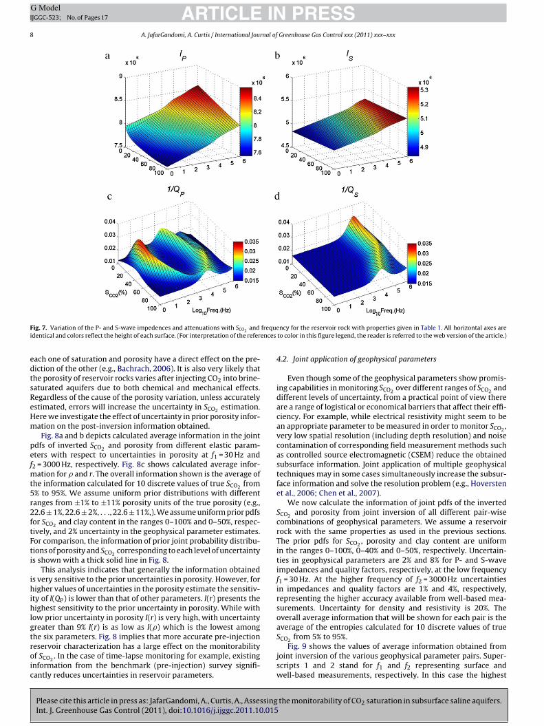
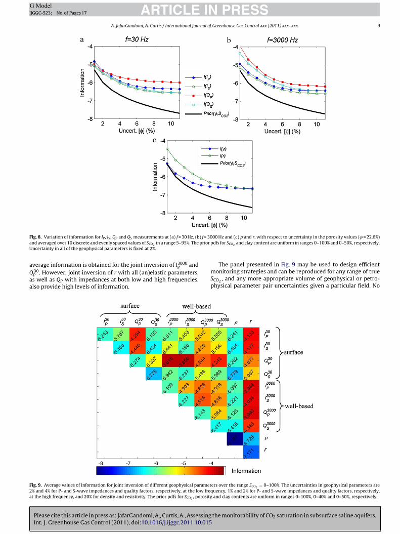

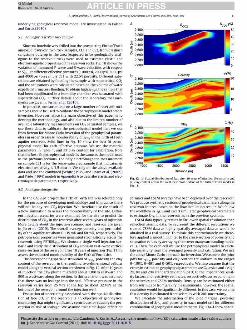

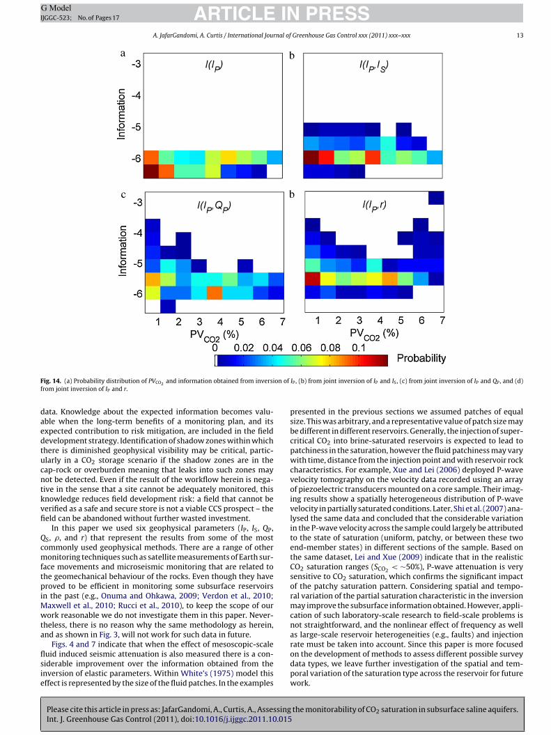


![Long-time analysis of nonlinearly perturbed wave equations via …hairer/preprints/wave.pdf · 2007-04-30 · Long-time analysis of nonlinearly perturbed wave equations 3 in [1,5],](https://static.documents.pub/doc/80x56/5e8e3d0b513c427c5a629df8/long-time-analysis-of-nonlinearly-perturbed-wave-equations-via-hairerpreprintswavepdf.jpg)


