Toward the understanding of partial-monitoring games ICML Workshop on Exploration & Exploitation Andr ´ as Antos G´ abor Bart´ ok D´ avid P ´ al Csaba Szepesv ´ ari University of Alberta E-mail: [email protected]Seattle, July 2, 2011 Szepesv ´ ari (UofA) Partial monitoring July 2, 2011 1 / 39
Transcript
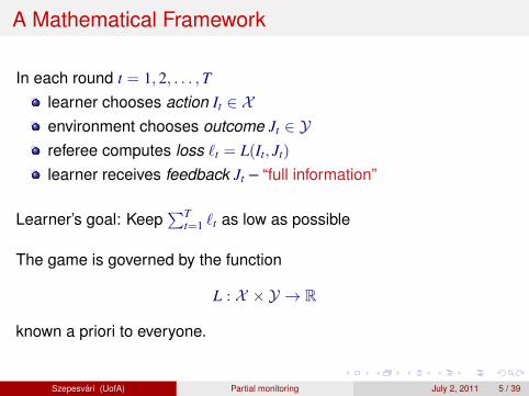
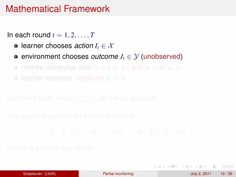
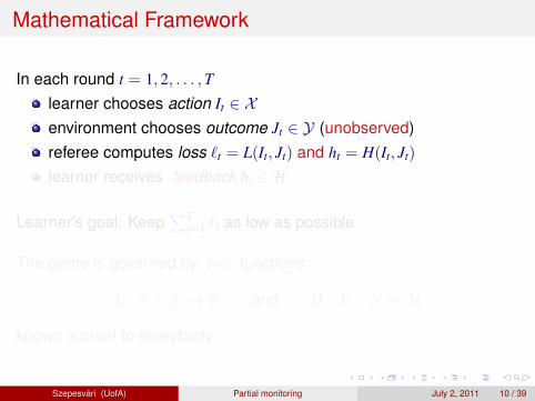
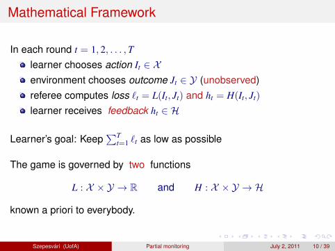
Toward the understanding of partial-monitoringgames
ICML Workshop on Exploration & Exploitation
Andras Antos Gabor Bartok David Pal Csaba Szepesvari
Szepesvari (UofA) Partial monitoring July 2, 2011 1 / 39
Contributions! !"# !"$ %&'()*+
!
%, -.*/0/)1)(2
34+5)(2
67+'()*+5
80.94(
:*1)'2;<)(=;
.4'*9+)>4.
?4=0@)*.;:*1)'2
80.94(;
:*1)'2;<A*
;.4'*9+)>4.
Off-policy learning with options and recognizersDoina Precup, Richard S. Sutton, Cosmin Paduraru, Anna J. Koop, Satinder Singh
McGill University, University of Alberta, University of Michigan
Options
Distinguished
region
Ideas and Motivation Background Recognizers Off-policy algorithm for options Learning w/o the Behavior Policy
Wall
Options• A way of behaving for a period of time
Models of options• A predictive model of the outcome of following the option• What state will you be in?• Will you still control the ball?• What will be the value of some feature?• Will your teammate receive the pass?• What will be the expected total reward along the way?• How long can you keep control of the ball?
Dribble Keepaway Pass
Options for soccer players could be
Options in a 2D world
The red and blue options
are mostly executed.
Surely we should be able
to learn about them from
this experience!
Experienced
trajectory
Off-policy learning• Learning about one policy while behaving according to another• Needed for RL w/exploration (as in Q-learning)• Needed for learning abstract models of dynamical systems
(representing world knowledge)• Enables efficient exploration• Enables learning about many ways of behaving at the same time
(learning models of options)
! a policy! a stopping condition
Non-sequential example
Problem formulation w/o recognizers
Problem formulation with recognizers
• One state
• Continuous action a ! [0, 1]
• Outcomes zi = ai
• Given samples from policy b : [0, 1] " #+
• Would like to estimate the mean outcome for a sub-region of the
action space, here a ! [0.7, 0.9]
Target policy ! : [0, 1] ! "+ is uniform within the region of interest
(see dashed line in figure below). The estimator is:
m! =1n
nX
i=1
!(ai)
b(ai)zi.
Theorem 1 Let A = a1, . . . ak ! A be a subset of all the
possible actions. Consider a fixed behavior policy b and let !A be
the class of policies that only choose actions from A, i.e., if!(a) > 0 then a " A. Then the policy induced by b and the binaryrecognizer cA is the policy with minimum-variance one-step
importance sampling corrections, among those in !A:
! as given by (1) = arg minp!!A
Eb
"
„
!(ai)
b(ai)
«2#
(2)
Proof: Using Lagrange multipliers
Theorem 2 Consider two binary recognizers c1 and c2, such that
µ1 > µ2. Then the importance sampling corrections for c1 have
lower variance than the importance sampling corrections for c2.
Off-policy learning
Let the importance sampling ratio at time step t be:
!t ="(st, at)
b(st, at)
The truncated n-step return, R(n)t , satisfies:
R(n)t = !t[rt+1 + (1 ! #t+1)R
(n!1)t+1 ].
The update to the parameter vector is proportional to:
!$t =h
R!t ! yt
i
""yt!0(1 ! #1) · · · !t!1(1 ! #t).
Theorem 3 For every time step t ! 0 and any initial state s,
Eb[!!t|s] = E![!!t|s].
Proof: By induction on n we show that
EbR(n)t |s = E!R
(n)t |s
which implies that EbR"t |s = E!(R"
t |s. The rest of the proof isalgebraic manipulations (see paper).
Implementation of off-policy learning for options
In order to avoid!! ! 0, we use a restart function g : S ! [0, 1](like in the PSD algorithm). The forward algorithm becomes:
!!t = (R!t " yt)#"yt
tX
i=0
gi"i..."t!1(1 " #i+1)...(1 " #t),
where gt is the extent of restarting in state st.
The incremental learning algorithm is the following:
• Initialize !0 = g0, e0 = !0!!y0
• At every time step t:
"t = #t (rt+1 + (1 " $t+1)yt+1) " yt
%t+1 = %t + &"tet
!t+1 = #t!t(1 " $t+1) + gt+1
et+1 = '#t(1 " $t+1)et + !t+1!!yt+1
References
Off-policy learning is tricky
• The Bermuda triangle
! Temporal-difference learning! Function approximation (e.g., linear)! Off-policy
• Leads to divergence of iterative algorithms! Q-learning diverges with linear FA! Dynamic programming diverges with linear FA
Baird's Counterexample
Vk(s) =
!(7)+2!(1)
terminal
state99%
1%
100%
Vk(s) =
!(7)+2!(2)
Vk(s) =
!(7)+2!(3)
Vk(s) =
!(7)+2!(4)
Vk(s) =
!(7)+2!(5)
Vk(s) =
2!(7)+!(6)
0
5
10
0 1000 2000 3000 4000 5000
10
10
/ -10
Iterations (k)
510
1010
010
-
-
Parametervalues, !k(i)
(log scale,
broken at !1)
!k(7)
!k(1) – !k(5)
!k(6)
Precup, Sutton & Dasgupta (PSD) algorithm
• Uses importance sampling to convert off-policy case to on-policy case• Convergence assured by theorem of Tsitsiklis & Van Roy (1997)• Survives the Bermuda triangle!
BUT!
• Variance can be high, even infinite (slow learning)• Difficult to use with continuous or large action spaces• Requires explicit representation of behavior policy (probability distribution)
Option formalism
An option is defined as a triple o = !I,!, ""
• I # S is the set of states in which the option can be initiated
• ! is the internal policy of the option
• " : S $ [0, 1] is a stochastic termination condition
We want to compute the reward model of option o:
EoR(s) = Er1 + r2 + . . . + rT |s0 = s, !, "
We assume that linear function approximation is used to represent
the model:
EoR(s) % #T $s = y
Baird, L. C. (1995). Residual algorithms: Reinforcement learning with function
approximation. In Proceedings of ICML.
Precup, D., Sutton, R. S. and Dasgupta, S. (2001). Off-policy temporal-difference
learning with function approximation. In Proceedings of ICML.
Sutton, R.S., Precup D. and Singh, S (1999). Between MDPs and semi-MDPs: A
framework for temporal abstraction in reinforcement learning. Artificial
Intelligence, vol . 112, pp. 181–211.
Sutton,, R.S. and Tanner, B. (2005). Temporal-difference networks. In Proceedings
of NIPS-17.
Sutton R.S., Rafols E. and Koop, A. (2006). Temporal abstraction in
temporal-difference networks”. In Proceedings of NIPS-18.
Tadic, V. (2001). On the convergence of temporal-difference learning with linear
function approximation. In Machine learning vol. 42.
Tsitsiklis, J. N., and Van Roy, B. (1997). An analysis of temporal-difference learning
with function approximation. IEEE Transactions on Automatic Control 42.
Acknowledgements
Theorem 4 If the following assumptions hold:
• The function approximator used to represent the model is a
state aggregrator
• The recognizer behaves consistently with the function
approximator, i.e., c(s, a) = c(p, a), !s " p
• The recognition probability for each partition, µ(p) is estimatedusing maximum likelihood:
µ(p) =N(p, c = 1)
N(p)
Then there exists a policy ! such that the off-policy learning
algorithm converges to the same model as the on-policy algorithm
using !.
Proof: In the limit, w.p.1, µ converges toP
s db(s|p)P
a c(p, a)b(s, a) where db(s|p) is the probability ofvisiting state s from partition p under the stationary distribution of b.
Let ! be defined to be the same for all states in a partition p:
!(p, a) = "(p, a)X
s
db(s|p)b(s, a)
! is well-defined, in the sense thatP
a !(s, a) = 1. Using Theorem3, off-policy updates using importance sampling corrections " willhave the same expected value as on-policy updates using !.
The authors gratefully acknowledge the ideas and encouragement
they have received in this work from Eddie Rafols, Mark Ring,
Lihong Li and other members of the rlai.net group. We thank Csaba
Szepesvari and the reviewers of the paper for constructive
comments. This research was supported in part by iCore, NSERC,
Alberta Ingenuity, and CFI.
The target policy ! is induced by a recognizer function
where µ(s) depends on the behavior policy b. If b is unknown,instead of µ we will use a maximum likelihood estimate
µ : S ! [0, 1], and importance sampling corrections will be definedas:
!(s, a) =c(s, a)
µ(s)
On-policy learning
If ! is used to generate behavior, then the reward model of anoption can be learned using TD-learning.
The n-step truncated return is:
R(n)t = rt+1 + (1 ! "t+1)R
(n!1)t+1 .
The #-return is defined as usual:
R!t = (1 ! #)
"X
n=1
#n!1R(n)t .
The parameters of the function approximator are updated on every
step proportionally to:
!$t =h
R!t ! yt
i
""yt(1 ! "1) · · · (1 ! "t).
• Recognizers reduce variance
• First off-policy learning algorithm for option models
• Off-policy learning without knowledge of the behavior
distribution
• Observations
– Options are a natural way to reduce the variance of
importance sampling algorithms (because of the termination
condition)
– Recognizers are a natural way to define options, especially
for large or continuous action spaces.
Contributions! !"# !"$ %&'()*+
!
%, -.*/0/)1)(2
34+5)(2
67+'()*+5
80.94(
:*1)'2;<)(=;
.4'*9+)>4.
?4=0@)*.;:*1)'2
80.94(;
:*1)'2;<A*
;.4'*9+)>4.
Off-policy learning with options and recognizersDoina Precup, Richard S. Sutton, Cosmin Paduraru, Anna J. Koop, Satinder Singh
McGill University, University of Alberta, University of Michigan
Options
Distinguished
region
Ideas and Motivation Background Recognizers Off-policy algorithm for options Learning w/o the Behavior Policy
Wall
Options• A way of behaving for a period of time
Models of options• A predictive model of the outcome of following the option• What state will you be in?• Will you still control the ball?• What will be the value of some feature?• Will your teammate receive the pass?• What will be the expected total reward along the way?• How long can you keep control of the ball?
Dribble Keepaway Pass
Options for soccer players could be
Options in a 2D world
The red and blue options
are mostly executed.
Surely we should be able
to learn about them from
this experience!
Experienced
trajectory
Off-policy learning• Learning about one policy while behaving according to another• Needed for RL w/exploration (as in Q-learning)• Needed for learning abstract models of dynamical systems
(representing world knowledge)• Enables efficient exploration• Enables learning about many ways of behaving at the same time
(learning models of options)
! a policy! a stopping condition
Non-sequential example
Problem formulation w/o recognizers
Problem formulation with recognizers
• One state
• Continuous action a ! [0, 1]
• Outcomes zi = ai
• Given samples from policy b : [0, 1] " #+
• Would like to estimate the mean outcome for a sub-region of the
action space, here a ! [0.7, 0.9]
Target policy ! : [0, 1] ! "+ is uniform within the region of interest
(see dashed line in figure below). The estimator is:
m! =1n
nX
i=1
!(ai)
b(ai)zi.
Theorem 1 Let A = a1, . . . ak ! A be a subset of all the
possible actions. Consider a fixed behavior policy b and let !A be
the class of policies that only choose actions from A, i.e., if!(a) > 0 then a " A. Then the policy induced by b and the binaryrecognizer cA is the policy with minimum-variance one-step
importance sampling corrections, among those in !A:
! as given by (1) = arg minp!!A
Eb
"
„
!(ai)
b(ai)
«2#
(2)
Proof: Using Lagrange multipliers
Theorem 2 Consider two binary recognizers c1 and c2, such that
µ1 > µ2. Then the importance sampling corrections for c1 have
lower variance than the importance sampling corrections for c2.
Off-policy learning
Let the importance sampling ratio at time step t be:
!t ="(st, at)
b(st, at)
The truncated n-step return, R(n)t , satisfies:
R(n)t = !t[rt+1 + (1 ! #t+1)R
(n!1)t+1 ].
The update to the parameter vector is proportional to:
!$t =h
R!t ! yt
i
""yt!0(1 ! #1) · · · !t!1(1 ! #t).
Theorem 3 For every time step t ! 0 and any initial state s,
Eb[!!t|s] = E![!!t|s].
Proof: By induction on n we show that
EbR(n)t |s = E!R
(n)t |s
which implies that EbR"t |s = E!(R"
t |s. The rest of the proof isalgebraic manipulations (see paper).
Implementation of off-policy learning for options
In order to avoid!! ! 0, we use a restart function g : S ! [0, 1](like in the PSD algorithm). The forward algorithm becomes:
!!t = (R!t " yt)#"yt
tX
i=0
gi"i..."t!1(1 " #i+1)...(1 " #t),
where gt is the extent of restarting in state st.
The incremental learning algorithm is the following:
• Initialize !0 = g0, e0 = !0!!y0
• At every time step t:
"t = #t (rt+1 + (1 " $t+1)yt+1) " yt
%t+1 = %t + &"tet
!t+1 = #t!t(1 " $t+1) + gt+1
et+1 = '#t(1 " $t+1)et + !t+1!!yt+1
References
Off-policy learning is tricky
• The Bermuda triangle
! Temporal-difference learning! Function approximation (e.g., linear)! Off-policy
• Leads to divergence of iterative algorithms! Q-learning diverges with linear FA! Dynamic programming diverges with linear FA
Baird's Counterexample
Vk(s) =
!(7)+2!(1)
terminal
state99%
1%
100%
Vk(s) =
!(7)+2!(2)
Vk(s) =
!(7)+2!(3)
Vk(s) =
!(7)+2!(4)
Vk(s) =
!(7)+2!(5)
Vk(s) =
2!(7)+!(6)
0
5
10
0 1000 2000 3000 4000 5000
10
10
/ -10
Iterations (k)
510
1010
010
-
-
Parametervalues, !k(i)
(log scale,
broken at !1)
!k(7)
!k(1) – !k(5)
!k(6)
Precup, Sutton & Dasgupta (PSD) algorithm
• Uses importance sampling to convert off-policy case to on-policy case• Convergence assured by theorem of Tsitsiklis & Van Roy (1997)• Survives the Bermuda triangle!
BUT!
• Variance can be high, even infinite (slow learning)• Difficult to use with continuous or large action spaces• Requires explicit representation of behavior policy (probability distribution)
Option formalism
An option is defined as a triple o = !I,!, ""
• I # S is the set of states in which the option can be initiated
• ! is the internal policy of the option
• " : S $ [0, 1] is a stochastic termination condition
We want to compute the reward model of option o:
EoR(s) = Er1 + r2 + . . . + rT |s0 = s, !, "
We assume that linear function approximation is used to represent
the model:
EoR(s) % #T $s = y
Baird, L. C. (1995). Residual algorithms: Reinforcement learning with function
approximation. In Proceedings of ICML.
Precup, D., Sutton, R. S. and Dasgupta, S. (2001). Off-policy temporal-difference
learning with function approximation. In Proceedings of ICML.
Sutton, R.S., Precup D. and Singh, S (1999). Between MDPs and semi-MDPs: A
framework for temporal abstraction in reinforcement learning. Artificial
Intelligence, vol . 112, pp. 181–211.
Sutton,, R.S. and Tanner, B. (2005). Temporal-difference networks. In Proceedings
of NIPS-17.
Sutton R.S., Rafols E. and Koop, A. (2006). Temporal abstraction in
temporal-difference networks”. In Proceedings of NIPS-18.
Tadic, V. (2001). On the convergence of temporal-difference learning with linear
function approximation. In Machine learning vol. 42.
Tsitsiklis, J. N., and Van Roy, B. (1997). An analysis of temporal-difference learning
with function approximation. IEEE Transactions on Automatic Control 42.
Acknowledgements
Theorem 4 If the following assumptions hold:
• The function approximator used to represent the model is a
state aggregrator
• The recognizer behaves consistently with the function
approximator, i.e., c(s, a) = c(p, a), !s " p
• The recognition probability for each partition, µ(p) is estimatedusing maximum likelihood:
µ(p) =N(p, c = 1)
N(p)
Then there exists a policy ! such that the off-policy learning
algorithm converges to the same model as the on-policy algorithm
using !.
Proof: In the limit, w.p.1, µ converges toP
s db(s|p)P
a c(p, a)b(s, a) where db(s|p) is the probability ofvisiting state s from partition p under the stationary distribution of b.
Let ! be defined to be the same for all states in a partition p:
!(p, a) = "(p, a)X
s
db(s|p)b(s, a)
! is well-defined, in the sense thatP
a !(s, a) = 1. Using Theorem3, off-policy updates using importance sampling corrections " willhave the same expected value as on-policy updates using !.
The authors gratefully acknowledge the ideas and encouragement
they have received in this work from Eddie Rafols, Mark Ring,
Lihong Li and other members of the rlai.net group. We thank Csaba
Szepesvari and the reviewers of the paper for constructive
comments. This research was supported in part by iCore, NSERC,
Alberta Ingenuity, and CFI.
The target policy ! is induced by a recognizer function
Where isdynamicpricing?Where shouldwe putG = (L,H)??How to play agame G?
Szepesvari (UofA) Partial monitoring July 2, 2011 16 / 39
Our Contributions
Characterization of 2×M and N × 2 games for adversarialenvironmentsCharacterization of all N ×M games for environments thatgenerate outcomes i.i.d.(stochastic environments)Any N ×M game falls into one of the four categories:
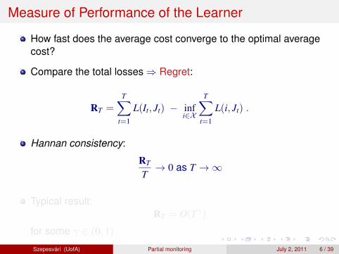
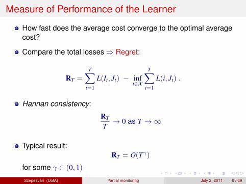
trivial RT = 0easy RT = Θ(
√T)
hard RT = Θ(T2/3)hopeless RT = Θ(T)
Szepesvari (UofA) Partial monitoring July 2, 2011 17 / 39
Outline
1 Partial Monitoring (what and why?)Prediction games (“full information setting”)Partial-monitoring
2 ResultsInformation, loss-estimationThe fundamental lemmaLower boundUpper bound
3 Conclusions and Open Problems
4 Bibliography
Szepesvari (UofA) Partial monitoring July 2, 2011 18 / 39
What Information Can We Collect?
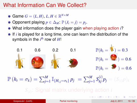
Game G = (L,H), L,H ∈ RN×M
Opponent playing p ∈ ∆M: P (Jt = j) = pj.What information does the player gain when playing action i?If i is played for a long time, one can learn the distribution of thesymbols in the ith row of H!
Szepesvari (UofA) Partial monitoring July 2, 2011 19 / 39
What Information Can We Collect?
Game G = (L,H), L,H ∈ RN×M
Opponent playing p ∈ ∆M: P (Jt = j) = pj.What information does the player gain when playing action i?If i is played for a long time, one can learn the distribution of thesymbols in the ith row of H!
0.1 0.6 0.2 0.1 P(ht = ) = 0.3
P(ht = ) = 0.6
P(ht = ) = 0.6
P (ht = σk) =∑M
j=1 IHi,j=σk pj =∑M
j=1 S(i)kj pj = (S(i)p)k
S(i): Signal matrix underlying action i
Szepesvari (UofA) Partial monitoring July 2, 2011 19 / 39
What is the Information Good For?
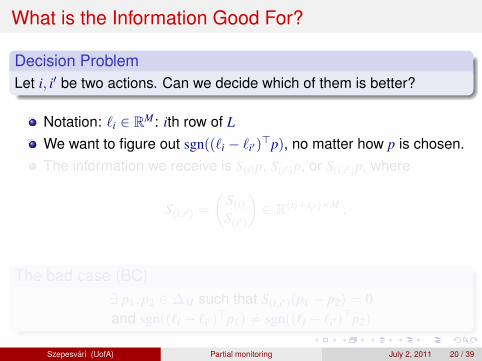
Decision ProblemLet i, i′ be two actions. Can we decide which of them is better?
Notation: `i ∈ RM: ith row of L
We want to figure out sgn((`i − `i′)>p), no matter how p is chosen.
The information we receive is S(i)p, S(i′)p, or S(i,i′)p, where
S(i,i′) =
(S(i)S(i′)
)∈ R(si+si′ )×M .
The bad case (BC)∃ p1, p2 ∈ ∆M such that S(i,i′)(p1 − p2) = 0and sgn((`i − `i′)
>p1) 6= sgn((`i − `i′)>p2)
Szepesvari (UofA) Partial monitoring July 2, 2011 20 / 39
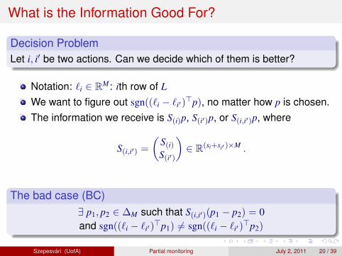
What is the Information Good For?
Decision ProblemLet i, i′ be two actions. Can we decide which of them is better?
Notation: `i ∈ RM: ith row of L
We want to figure out sgn((`i − `i′)>p), no matter how p is chosen.
The information we receive is S(i)p, S(i′)p, or S(i,i′)p, where
S(i,i′) =
(S(i)S(i′)
)∈ R(si+si′ )×M .
The bad case (BC)∃ p1, p2 ∈ ∆M such that S(i,i′)(p1 − p2) = 0and sgn((`i − `i′)
>p1) 6= sgn((`i − `i′)>p2)
Szepesvari (UofA) Partial monitoring July 2, 2011 20 / 39
Outline
1 Partial Monitoring (what and why?)Prediction games (“full information setting”)Partial-monitoring
2 ResultsInformation, loss-estimationThe fundamental lemmaLower boundUpper bound
3 Conclusions and Open Problems
4 Bibliography
Szepesvari (UofA) Partial monitoring July 2, 2011 21 / 39
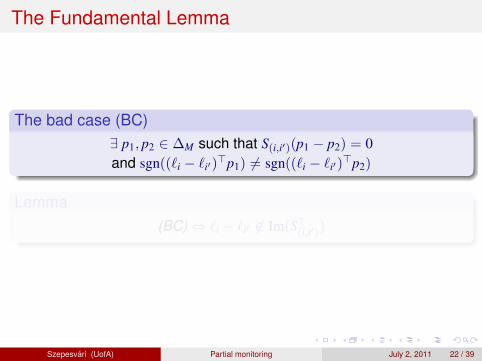
The Fundamental Lemma
The bad case (BC)∃ p1, p2 ∈ ∆M such that S(i,i′)(p1 − p2) = 0and sgn((`i − `i′)
>p1) 6= sgn((`i − `i′)>p2)
Lemma(BC)⇔ `i − `i′ 6∈ Im(S>(i,i′))
Szepesvari (UofA) Partial monitoring July 2, 2011 22 / 39
The Fundamental Lemma
The bad case (BC)∃ p1, p2 ∈ ∆M such that S(i,i′)(p1 − p2) = 0and sgn((`i − `i′)
>p1) 6= sgn((`i − `i′)>p2)
Lemma(BC)⇔ `i − `i′ 6∈ Im(S>(i,i′))
Szepesvari (UofA) Partial monitoring July 2, 2011 22 / 39
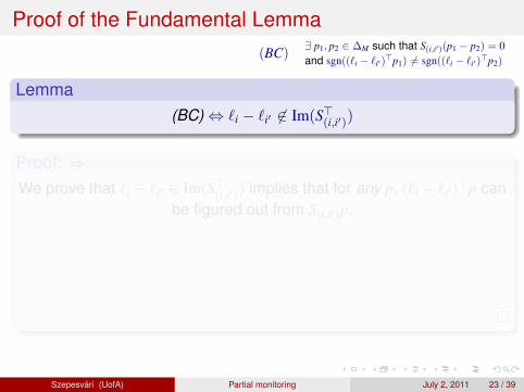
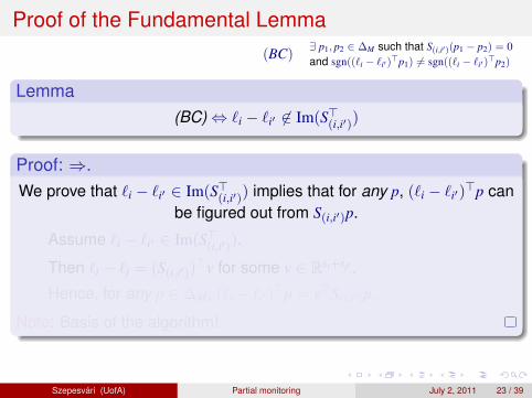
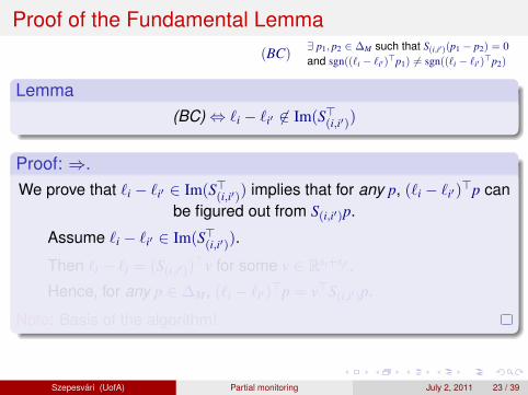
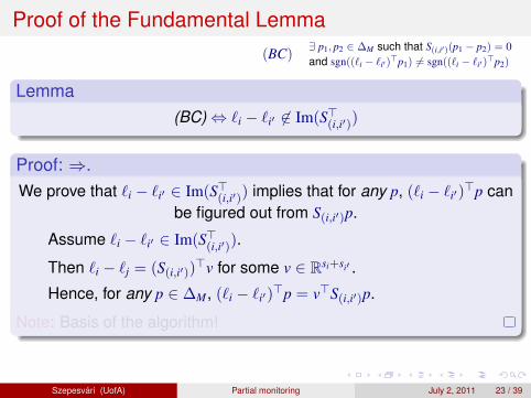
Proof of the Fundamental Lemma(BC)
∃ p1, p2 ∈ ∆M such that S(i,i′)(p1 − p2) = 0and sgn((`i − `i′)
>p1) 6= sgn((`i − `i′)>p2)
Lemma(BC)⇔ `i − `i′ 6∈ Im(S>(i,i′))
Proof: ⇒.We prove that `i − `i′ ∈ Im(S>(i,i′)) implies that for any p, (`i − `i′)
>p canbe figured out from S(i,i′)p.
Assume `i − `i′ ∈ Im(S>(i,i′)).
Then `i − `j = (S(i,i′))>v for some v ∈ Rsi+si′ .
Hence, for any p ∈ ∆M, (`i − `i′)>p = v>S(i,i′)p.
Note: Basis of the algorithm!
Szepesvari (UofA) Partial monitoring July 2, 2011 23 / 39
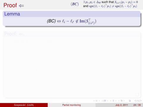
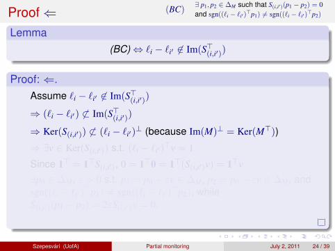
Proof⇐ (BC)∃ p1, p2 ∈ ∆M such that S(i,i′)(p1 − p2) = 0and sgn((`i − `i′)
Szepesvari (UofA) Partial monitoring July 2, 2011 24 / 39
Illustration
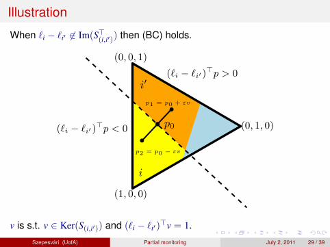
When `i − `i′ 6∈ Im(S>(i,i′)) then (BC) holds.
(1, 0, 0)
(0, 1, 0)
(0, 0, 1)
i
i′(`i − `i′)>p < 0
(`i − `i′)>p > 0
p0
p1 = p0 + εv
p2 = p0 − εv
v is s.t. v ∈ Ker(S(i,i′)) and (`i − `i′)>v = 1.
Szepesvari (UofA) Partial monitoring July 2, 2011 25 / 39
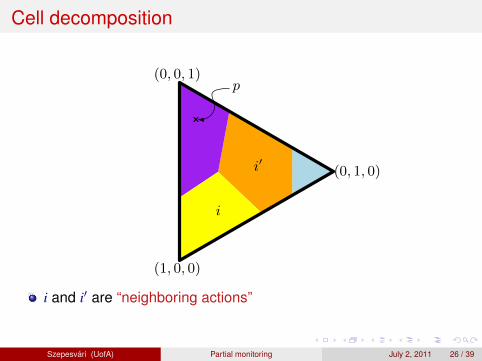
Cell decomposition
(1, 0, 0)
(0, 1, 0)
(0, 0, 1)p
i
i′
i and i′ are “neighboring actions”
Szepesvari (UofA) Partial monitoring July 2, 2011 26 / 39
Outline
1 Partial Monitoring (what and why?)Prediction games (“full information setting”)Partial-monitoring
2 ResultsInformation, loss-estimationThe fundamental lemmaLower boundUpper bound
3 Conclusions and Open Problems
4 Bibliography
Szepesvari (UofA) Partial monitoring July 2, 2011 27 / 39
Lower Bound
TheoremIf there exists i, i′ actions which are neighbors and `i − `i′ 6∈ Im(S>(i,i′))
then the RT = Ω(T2/3).
Proof.Follows from the Fundamental Lemma:∃p1, p2 ∈ ∆M s.t. p1 makes i optimal, p2 makes i′ optimal and thereis no way to distinguish between p1 and p2 based on theobservations.If there is no third action, the game is hopelessIf there is a third action that can help distinguishing p1 and p2 thenit will be costly to use it whenever p is either p1 or p2.
Szepesvari (UofA) Partial monitoring July 2, 2011 28 / 39
Illustration
When `i − `i′ 6∈ Im(S>(i,i′)) then (BC) holds.
(1, 0, 0)
(0, 1, 0)
(0, 0, 1)
i
i′
(`i − `i′)>p < 0
(`i − `i′)>p > 0
p0
p1 = p0 + εv
p2 = p0 − εv
v is s.t. v ∈ Ker(S(i,i′)) and (`i − `i′)>v = 1.
Szepesvari (UofA) Partial monitoring July 2, 2011 29 / 39
Outline
1 Partial Monitoring (what and why?)Prediction games (“full information setting”)Partial-monitoring
2 ResultsInformation, loss-estimationThe fundamental lemmaLower boundUpper bound
3 Conclusions and Open Problems
4 Bibliography
Szepesvari (UofA) Partial monitoring July 2, 2011 30 / 39
Toward the Upper Bound
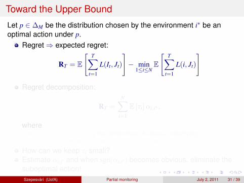
Let p ∈ ∆M be the distribution chosen by the environment i∗ be anoptimal action under p.
Regret⇒ expected regret:
RT = E
[T∑
t=1
L(It, Jt)
]− min
1≤i≤NE
[T∑
t=1
L(i, Jt)
]
Regret decomposition:
RT =
N∑
i=1
E [τi]αi,i∗ ,
whereI αi,i′ = (`i − `i′)
>p is the difference of losses underlying i, i′,I τi is the number of times action i is played.
How can we keep τi small?Estimate αi,i′ and when sgn(αi,i′) becomes obvious, eliminate thesuboptimal action!Szepesvari (UofA) Partial monitoring July 2, 2011 31 / 39
Toward the Upper Bound
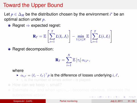
Let p ∈ ∆M be the distribution chosen by the environment i∗ be anoptimal action under p.
Regret⇒ expected regret:
RT = E
[T∑
t=1
L(It, Jt)
]− min
1≤i≤NE
[T∑
t=1
L(i, Jt)
]
Regret decomposition:
RT =
N∑
i=1
E [τi]αi,i∗ ,
whereI αi,i′ = (`i − `i′)
>p is the difference of losses underlying i, i′,I τi is the number of times action i is played.
How can we keep τi small?Estimate αi,i′ and when sgn(αi,i′) becomes obvious, eliminate thesuboptimal action!Szepesvari (UofA) Partial monitoring July 2, 2011 31 / 39
Toward the Upper Bound
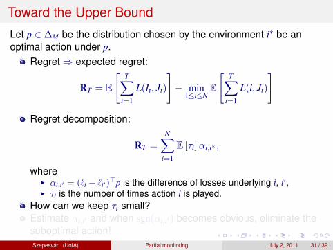
Let p ∈ ∆M be the distribution chosen by the environment i∗ be anoptimal action under p.
Regret⇒ expected regret:
RT = E
[T∑
t=1
L(It, Jt)
]− min
1≤i≤NE
[T∑
t=1
L(i, Jt)
]
Regret decomposition:
RT =
N∑
i=1
E [τi]αi,i∗ ,
whereI αi,i′ = (`i − `i′)
>p is the difference of losses underlying i, i′,I τi is the number of times action i is played.
How can we keep τi small?Estimate αi,i′ and when sgn(αi,i′) becomes obvious, eliminate thesuboptimal action!Szepesvari (UofA) Partial monitoring July 2, 2011 31 / 39
Toward the Upper Bound
Let p ∈ ∆M be the distribution chosen by the environment i∗ be anoptimal action under p.
Regret⇒ expected regret:
RT = E
[T∑
t=1
L(It, Jt)
]− min
1≤i≤NE
[T∑
t=1
L(i, Jt)
]
Regret decomposition:
RT =
N∑
i=1
E [τi]αi,i∗ ,
whereI αi,i′ = (`i − `i′)
>p is the difference of losses underlying i, i′,I τi is the number of times action i is played.
How can we keep τi small?Estimate αi,i′ and when sgn(αi,i′) becomes obvious, eliminate thesuboptimal action!Szepesvari (UofA) Partial monitoring July 2, 2011 31 / 39
Constructing Good Estimates
Assume that for every neighboring action i, i′, `i − `i′ ∈ Im(S>(i,i′))How to exploit this?If i, i′ are neighbors, ∃v(i,i′) ∈ Rsi+si′ s.t.
`i − `i′ = S>(i,i′)v(i,i′)
Estimate:I Assume the learner tried i, i′ n-times, let q(i,i′) be the corresponding
empirical distribution over the observations.I Estimate αi,i′ using
αi,i′ = v>(i,i′)q(i,i′)
I This works because q(i,i′) ≈ S(i,i′)p and soαi,i′ = v>(i,i′)q(i,i′) ≈ v>(i,i′)S(i,i′)p = (`i − `i′)
>pWhen i, i′ are not neighbors, form a chain i = i0, i1, . . . , iK = i′ ofneighbors and use αi,i′ =
∑K−1k=0 αik,ik+1 .
Szepesvari (UofA) Partial monitoring July 2, 2011 32 / 39
When Should the Learner Stop Using an Action?
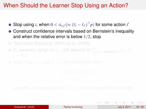
Stop using i, when 0 < αi,i′(≈ (`i − `i′)>p) for some action i′
Construct confidence intervals based on Bernstein’s inequalityand when the relative error is below 1/2, stop“Bernstein Stopping” (Mnih et al., 2008)C. variance, range of αi,i′ will depend on
∑(i,i′) neighbors ‖vi,i′‖s
s,s = 1, 2
Assuming αi,i′ , w.p. 1− δ, this rule stops after
C1 log(C2/(δαi,i′))
α2i,i′
samples, for appropriate C1,C2 > 0 (game-specific) constants.
Szepesvari (UofA) Partial monitoring July 2, 2011 33 / 39
When Should the Learner Stop Using an Action?
Stop using i, when 0 < αi,i′(≈ (`i − `i′)>p) for some action i′
Construct confidence intervals based on Bernstein’s inequalityand when the relative error is below 1/2, stop“Bernstein Stopping” (Mnih et al., 2008)C. variance, range of αi,i′ will depend on
∑(i,i′) neighbors ‖vi,i′‖s
s,s = 1, 2
Assuming αi,i′ , w.p. 1− δ, this rule stops after
C1 log(C2/(δαi,i′))
α2i,i′
samples, for appropriate C1,C2 > 0 (game-specific) constants.
Szepesvari (UofA) Partial monitoring July 2, 2011 33 / 39
Finishing the Upper Bound
RT =∑N
i=1 E [τi]αi,i∗
Further, when the stopping rules do not fail..
N∑
i=1
τiαi,i∗ ≤∑
i:αi,i∗≥α0
C1 log(C2/(δαi,i∗))
α2i,i∗
αi,i∗ + α0
∑
i:αi,i∗<α0
τi
≤ C1Nlog(C2/(δα0))
α0+ α0T
Choose α0 =√
C1N/T to get
N∑
i=1
τiαi,i∗ ≤√
C1NT(1 + log(C2/(δα0))) .
Szepesvari (UofA) Partial monitoring July 2, 2011 34 / 39
Algorithm – BALATON
BALATON ≡ Bandit based loss annihilation
1 Repeat while there is more than one “alive” action:2 Estimate loss differences between alive actions3 When some estimate substantially differs from zero, kill the
suboptimal action4 Play the remaining action until the end
Szepesvari (UofA) Partial monitoring July 2, 2011 35 / 39
The Main Result
TheoremAny N ×M game falls into one of the four categories:
trivial RT = 0easy RT = Θ(
√T)
hard RT = Θ(T2/3)hopeless RT = Θ(T)
Szepesvari (UofA) Partial monitoring July 2, 2011 36 / 39
Summary for Finite, Stochastic Games
0 1
1
1/2
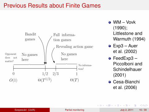
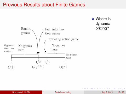
O(1) Θ(T 1/2) Θ(T )
Full informa-tion games
Banditgames
2/3
︷ ︸︸ ︷
No gameshere
Revealing action game
No informa-
tion!
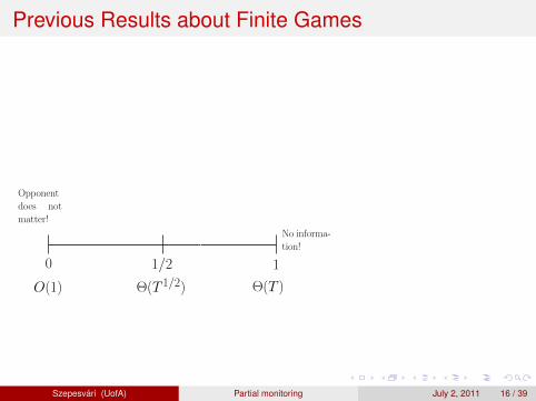
Opponent
does not
matter!︷ ︸︸ ︷︷ ︸︸ ︷
Any game is at 0, 1/2, 2/3 or 1
There is a computationally efficient way of determining where agiven game fallsExample: Dynamic pricing is at 2/3 (new!)If the game is “easy” (at 1/2), one should use BALATON
If the game is “hard” (at 2/3), one should use FEEDEXP3
Szepesvari (UofA) Partial monitoring July 2, 2011 37 / 39
Summary for Finite, Stochastic Games
0 1
1
1/2
O(1) Θ(T 1/2) Θ(T )
Full informa-tion games
Banditgames
2/3
︷ ︸︸ ︷
No gameshere
Revealing action game
No informa-
tion!
Opponent
does not
matter!︷ ︸︸ ︷︷ ︸︸ ︷
Any game is at 0, 1/2, 2/3 or 1
There is a computationally efficient way of determining where agiven game fallsExample: Dynamic pricing is at 2/3 (new!)If the game is “easy” (at 1/2), one should use BALATON
If the game is “hard” (at 2/3), one should use FEEDEXP3
Szepesvari (UofA) Partial monitoring July 2, 2011 37 / 39
Conclusions
Full characterization of stochastic partial monitoring gamesHardness depends on whether there exist neighboring actionswhose loss difference cannot be estimated locallyOpen question: Does this extend to the adversarial case?Conjecture: YesWANTED: Good algorithm, with O(
√T) regret when local
observability holdsOther questions:
I Dependence on other parameters: Number of actions, number ofoutcomes, the algebraic properties of (L,H)
I Infinite action spaces, infinite outcome spacesI Between bandit and full information: See Ohad Samir’s talk! ,I . . .
Szepesvari (UofA) Partial monitoring July 2, 2011 38 / 39
For Further Reading
Auer, P., Cesa-Bianchi, N., Freund, Y., andSchapire, R. (2002). The nonstochasticmultiarmed bandit problem. SIAM Journalon Computing, 32:48–77.
Cesa-Bianchi, N., Lugosi, G., and Stoltz, G.(2006). Regret minimization under partialmonitoring. Mathematics of OperationsResearch, 31:562–580.
Littlestone, N. and Warmuth, M. (1994). Theweighted majority algorithm. Informationand Computation, 108:212–261.
Mnih, V., Szepesvari, C., and Audibert, J.-Y.(2008). Empirical Bernstein stopping. In
Cohen, W. W., McCallum, A., and Roweis,S. T., editors, ICML 2008, pages 672–679.ACM.
Piccolboni, A. and Schindelhauer, C. (2001).Discrete prediction games with arbitraryfeedback and loss. In Helmbold, D. andWilliamson, B., editors, COLT2001/EuroCOLT 2001, volume 2111 ofLecture Notes in Computer Science, pages208–223. Springer.
Vovk, V. (1990). Aggregating strategies. InCOLT 1990, pages 371—383.
Szepesvari (UofA) Partial monitoring July 2, 2011 39 / 39