Product Traceability and Uncertainty for the Ozone Profile Differential Absorption Lidar Product Version 0.1.10 GAIA-CLIM Gap Analysis for Integrated Atmospheric ECV Climate Monitoring Mar 2015 - Feb 2018 A Horizon 2020 project; Grant agreement: 640276 Date: 20 January 2018 Dissemination level: Final Work Package 2; Compiled by Arnoud Apituley, Anne van Gijsel (KNMI)
Transcript
Product Traceability and Uncertainty
for the Ozone Profile Differential
Absorption Lidar Product
Version 0.1.10
GAIA-CLIM
Gap Analysis for Integrated
Atmospheric ECV Climate Monitoring
Mar 2015 - Feb 2018
A Horizon 2020 project; Grant agreement: 640276
Date: 20 January 2018
Dissemination level: Final
Work Package 2; Compiled by
Arnoud Apituley, Anne van Gijsel (KNMI)
Table of Contents
1 Version history ............................................................................................................................. 3
For general guidance see the Guide to Uncertainty in Measurement & its Nomenclature, published
as part of the GAIA-CLIM project.
This document is a measurement product technical document which should be stand-alone i.e.
intelligible in isolation. Reference to external sources (preferably peer-reviewed) and
documentation from previous studies is clearly expected and welcomed, but with sufficient
explanatory content in the GAIA CLIM document not to necessitate the reading of all these
reference documents to gain a clear understanding of the GAIA CLIM product and associated
uncertainties entered into the Virtual Observatory (VO).
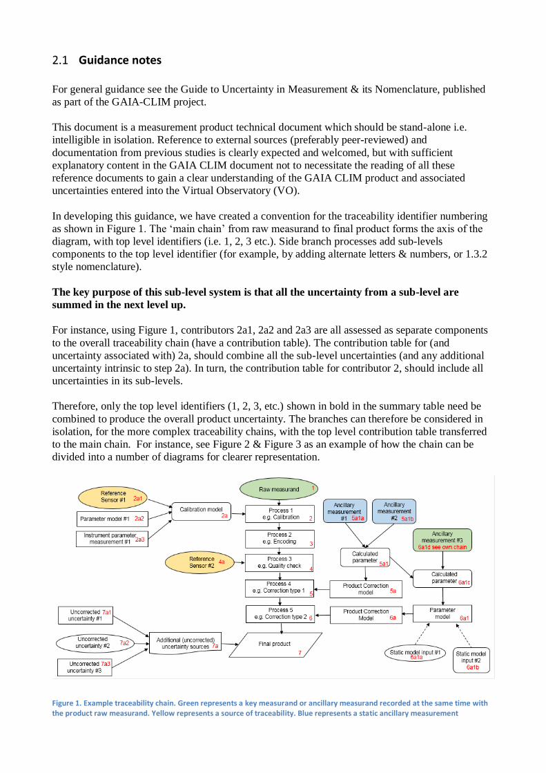
In developing this guidance, we have created a convention for the traceability identifier numbering
as shown in Figure 1. The ‘main chain’ from raw measurand to final product forms the axis of the
diagram, with top level identifiers (i.e. 1, 2, 3 etc.). Side branch processes add sub-levels
components to the top level identifier (for example, by adding alternate letters & numbers, or 1.3.2
style nomenclature).
The key purpose of this sub-level system is that all the uncertainty from a sub-level are
summed in the next level up.
For instance, using Figure 1, contributors 2a1, 2a2 and 2a3 are all assessed as separate components
to the overall traceability chain (have a contribution table). The contribution table for (and
uncertainty associated with) 2a, should combine all the sub-level uncertainties (and any additional
uncertainty intrinsic to step 2a). In turn, the contribution table for contributor 2, should include all
uncertainties in its sub-levels.
Therefore, only the top level identifiers (1, 2, 3, etc.) shown in bold in the summary table need be
combined to produce the overall product uncertainty. The branches can therefore be considered in
isolation, for the more complex traceability chains, with the top level contribution table transferred
to the main chain. For instance, see Figure 2 & Figure 3 as an example of how the chain can be
divided into a number of diagrams for clearer representation.
Figure 1. Example traceability chain. Green represents a key measurand or ancillary measurand recorded at the same time with the product raw measurand. Yellow represents a source of traceability. Blue represents a static ancillary measurement
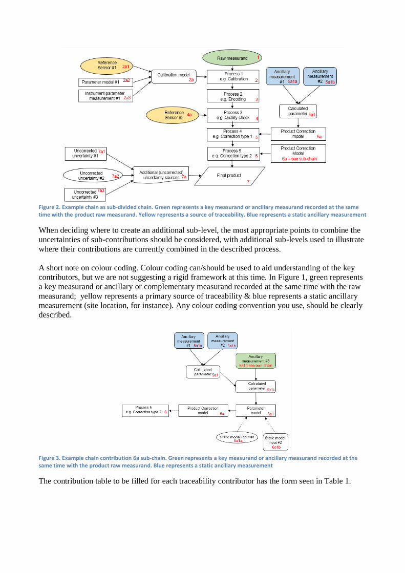
Figure 2. Example chain as sub-divided chain. Green represents a key measurand or ancillary measurand recorded at the same time with the product raw measurand. Yellow represents a source of traceability. Blue represents a static ancillary measurement
When deciding where to create an additional sub-level, the most appropriate points to combine the
uncertainties of sub-contributions should be considered, with additional sub-levels used to illustrate
where their contributions are currently combined in the described process.
A short note on colour coding. Colour coding can/should be used to aid understanding of the key
contributors, but we are not suggesting a rigid framework at this time. In Figure 1, green represents
a key measurand or ancillary or complementary measurand recorded at the same time with the raw
measurand; yellow represents a primary source of traceability & blue represents a static ancillary
measurement (site location, for instance). Any colour coding convention you use, should be clearly
described.
Figure 3. Example chain contribution 6a sub-chain. Green represents a key measurand or ancillary measurand recorded at the same time with the product raw measurand. Blue represents a static ancillary measurement
The contribution table to be filled for each traceability contributor has the form seen in Table 1.
Table 1. The contributor table.
Information / data Type / value / equation Notes / description
Name of effect
Contribution identifier
Measurement equation
parameter(s) subject to effect
Contribution subject to effect
(final product or sub-tree
intermediate product)
Time correlation extent & form
Other (non-time) correlation
extent & form
Uncertainty PDF shape
Uncertainty & units
Sensitivity coefficient
Correlation(s) between affected
parameters
Element/step common for all
sites/users?
Traceable to …
Validation
Name of effect – The name of the contribution. Should be clear, unique and match the description
in the traceability diagram.
Contribution identifier - Unique identifier to allow reference in the traceability chains.
Measurement equation parameter(s) subject to effect – The part of the measurement equation
influenced by this contribution. Ideally, the equation into which the element contributes.
Contribution subject to effect – The top level measurement contribution affected by this
contribution. This can be the main product (if on the main chain), or potentially the root of a side
branch contribution. It will depend on how the chain has been sub-divided.
Time correlation extent & form – The form & extent of any correlation this contribution has in
time.
Other (non-time) correlation extent & form – The form & extent of any correlation this
contribution has in a non-time domain. For example, spatial or spectral.
Uncertainty PDF shape – The probability distribution shape of the contribution, Gaussian/Normal
Rectangular, U-shaped, log-normal or other. If the form is not known, a written description is
sufficient.
Uncertainty & units – The uncertainty value, including units and confidence interval. This can be
a simple equation, but should contain typical values.
Sensitivity coefficient – Coefficient multiplied by the uncertainty when applied to the measurement
equation.
Correlation(s) between affected parameters – Any correlation between the parameters affected
by this specific contribution. If this element links to the main chain by multiple paths within the
traceability chain, it should be described here. For instance, SZA or surface pressure may be used
separately in a number of models & correction terms that are applied to the product at different
points in the processing. See Figure 1, contribution 5a1, for an example.
Element/step common for all sites/users – Is there any site-to-site/user-to-user variation in the
application of this contribution?
Traceable to – Describe any traceability back towards a primary/community reference.
Validation – Any validation activities that have been performed for this element?
3 Introduction This document presents the Product Traceabililty and Uncertainty (PTU) information for the ozone
profile differential absorption lidar product. The aim of this document is to provide supporting
information for the users of this product within the GAIA-CLIM VO. The uncertainty and
traceability information contained in this document is based on the details given in LeBlanc et al.
(2016b).
LeBlanc et al. (2016b) describe an approach for the definition, propagation, and reporting of
uncertainty in the ozone differential absorption lidar data products contributing to the Network for
the Detection of Atmospheric Composition Change (NDACC) database. One essential aspect of the
proposed approach is the propagation in parallel of all independent uncertainty components through
the data processing chain before they are combined together to form the ozone combined standard
uncertainty.
The independent uncertainty components contributing to the overall budget include random noise
associated with signal detection, uncertainty due to saturation correction, background noise
extraction, the absorption cross sections of O3, NO2 , SO2 , and O2 , the molecular extinction cross
sections, and the number densities of the air, NO2, and SO2. The expression of the individual
uncertainty components and their step-by-step propagation through the ozone differential absorption
lidar (DIAL) processing chain are thoroughly estimated. All sources of uncertainty except detection
noise imply correlated terms in the vertical dimension, which requires knowledge of the covariance
matrix when the lidar signal is vertically filtered. In addition, the covariance terms must be taken
into account if the same detection hardware is shared by the lidar receiver channels at the absorbed
and non-absorbed wavelengths.
The ozone uncertainty budget is presented as much as possible in a generic form (i.e., as a function
of instrument performance and wavelength) so that all NDACC ozone DIAL investigators across
the network can estimate, for their own instrument and in a straightforward manner, the expected
impact of each reviewed uncertainty component.
In the example of a stratospheric ozone DIAL after optimal combination of three DIAL wavelength
pairs, the ozone number density standard uncertainty results mainly from three components:
Rayleigh extinction cross section differential at the bottom of the profile, ozone absorption cross
section differential in the middle of the profile, and detection noise at the top of the profile. For the
derived ozone mixing ratio, the uncertainty component associated with the a priori use of ancillary
air pressure can become abruptly important above 30 km as a result of the transition between the a
priori use of radiosonde measurement (z < 30 km) and the a priori use of the NCEP analysis (z >
30 km). The dominant source of ozone mixing ratio uncertainty above 45 km is detection noise
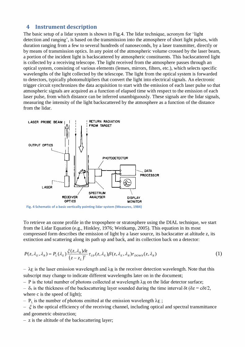
4 Instrument description The basic setup of a lidar system is shown in Fig.4. The lidar technique, acronym for ‘light
detection and ranging’, is based on the transmission into the atmosphere of short light pulses, with
duration ranging from a few to several hundreds of nanoseconds, by a laser transmitter, directly or
by means of transmission optics. In any point of the atmospheric volume crossed by the laser beam,
a portion of the incident light is backscattered by atmospheric constituents. This backscattered light
is collected by a receiving telescope. The light received from the atmosphere passes through an
optical system, consisting of various elements (lenses, mirrors, filters, etc.), which selects specific
wavelengths of the light collected by the telescope. The light from the optical system is forwarded
to detectors, typically photomultipliers that convert the light into electrical signals. An electronic
trigger circuit synchronizes the data acquisition to start with the emission of each laser pulse so that
atmospheric signals are acquired as a function of elapsed time with respect to the emission of each
laser pulse, from which distance can be inferred unambiguously. These signals are the lidar signals,
measuring the intensity of the light backscattered by the atmosphere as a function of the distance
from the lidar.
To retrieve an ozone profile in the troposphere or stratosphere using the DIAL technique, we start
from the Lidar Equation (e.g., Hinkley, 1976; Weitkamp, 2005). This equation in its most
compressed form describes the emission of light by a laser source, its backscatter at altitude z, its
extinction and scattering along its path up and back, and its collection back on a detector:
),(),,(),(
),()(),,(
2 RDOWNREEUP
L
RELRE zzz
zz
zzPzP
(1)
– λE is the laser emission wavelength and λR is the receiver detection wavelength. Note that this
subscript may change to indicate different wavelengths later on in the document;
– P is the total number of photons collected at wavelength λR on the lidar detector surface;
– δz is the thickness of the backscattering layer sounded during the time interval δt (δz = cδt/2,
where c is the speed of light);
– PL is the number of photons emitted at the emission wavelength λE ;
– is the optical efficiency of the receiving channel, including optical and spectral transmittance
and geometric obstruction;
– z is the altitude of the backscattering layer;
Fig. 4 Schematic of a basic vertically pointing lidar system (Measures, 1984)
– zL is the altitude of the lidar (laser and receiver assumed to be at the same altitude);
– β is the total backscatter coefficient (including particulate βP and molecular βM backscatter);
– τUP is the optical thickness integrated along the outgoing beam path between the lidar and the
scattering altitude z, and is defined as
z
z i
iEiEPaEMUP
L
dzzNzzzNz ')'(),'(),'()'()(exp)( (2)
– τDOWN is the optical thickness integrated along the returning beam path between the scattering
altitude z and the lidar receiver, and is defined as
z
z i
iRiRPaRMDOWN
L
dzzNzzzNz ')'(),'(),'()'()(exp)( (3)
where σM is the molecular extinction cross section due to Rayleigh scattering (Strutt, 1899)
(hereafter called “Rayleigh cross section” for brevity), Na is the air number density, αP is the
particulate extinction coefficient, σi is the absorption cross section of absorbing constituent i, and Ni
is the number density of absorbing constituent i. For the altitude range of interest of the ozone
DIAL measurements, the Rayleigh cross sections can be considered constant with altitude, and
therefore depend only on wavelength. The absorption cross sections, however, are in most cases
temperature-dependent, and should be taken as a function of both altitude and wavelength.
In the DIAL technique we consider the lidar signals measured at two different wavelengths, the
light at one wavelength being more absorbed by the target species (here, ozone) than the light at the
other wavelength (Mégie et al., 1977). Using the notation ON for the most absorbed wavelength,
and OFF for the least absorbed wavelength, Eq. (1) can be re-written for each of the emitted
wavelength:
),(),,(),(
)()()( 221121
zzz
zz
zzPzP DOWNUP
L
ONLON
(4)
),(),,(),(
)()()( 443323
zzz
zz
zzPzP DOWNUP
L
OFFLOFF
(5)
The emitted and received wavelength subscripts have been modified as follows:
1 and 2 are the emitted and received “ON” wavelengths respectively
3 and 4 are the emitted and received “OFF” wavelengths respectively
To obtain ozone number density NO3 , Eqs. (4)–(5) are rearranged and subsequently the vertical
derivative of the logarithm of the ratio of the lidar signals measured at the ON and OFF
wavelengths (Mégie et al., 1977):
)()()()()()(
)(
)(ln
)(
1)(
3
3 zzzzNzzNzP
zP
zzzN P
ig
igigaM
ON
OFF
O
O
(6)
The ozone DIAL measurement model depends on the choice of the theoretical equations used as
well as their implementation to the real world, i.e., after considering all the caveats associated with
the design, setup, and operation of an actual lidar instrument. Equation (6) relates to the expected
number of photons reaching the lidar detectors (PON and POFF), not the actual raw lidar signals
recorded in the data files by a real instrument. Its practical implementation for the retrieval of ozone
therefore requires, on one hand the addition of several signal correction procedures and numerical
transformations that depend on the instrumentation, and on the other hand, the development of
approximations and/or the adoption of assumptions aimed to reduce the complexity of the
measurement model.
In this context, uncertainty components associated with particulate extinction and backscatter (αP
and β terms in Eq. 6) will not be considered here. Their contribution is negligible in a cloud-free,
“clean” atmosphere, which is mostly true for altitudes above 35 km (e.g., Godin-Beekmann et al.,
2003), and in most cases of clear-sky, free-tropospheric ozone DIAL measurements for which the
wavelength differential is small (Papayannis et al., 1990; McDermid et al., 2002). When present and
non-negligible, the contribution of particulate extinction and backscatter is highly variable from site
to site, time to time, and highly dependent on the nature and quantity of the particulate matter at the
time of measurement. A number of rather different assessment methods exist (for a review, see e.g.,
Eisele and Trickl, 2005). Proposing a meaningful standardized treatment of this uncertainty
component is therefore complex and beyond the scope of the present work.
Similarly, uncertainty due to incomplete beam-telescope overlap correction (η term in Eq. 6) is
instrument-dependent and often time-dependent for the same instrument. Therefore, no standardized
formulation is provided here. However an example of treatment is provided in the ISSI team report
(Leblanc et al., 2016c).
The detectors quantum efficiencies and the effects of the data recorders (e.g., sky and electronic
background noise, signal saturation) must be taken into account. Due to the diversity of lidar
instrumentation, it is not possible to provide a single expression for the parametrization of these
effects and obtain a unique, real-world version of Eq. (6) applicable to all systems. However, we
use standardized expressions that characterize the most commonly found cases, with the idea that
the proposed approach for the propagation of uncertainty can be similarly applied to other cases.
Specifically, to transition from a theoretical to a real ozone DIAL measurement model, we apply the
following transformations.
• For each lidar receiver channel, the actual raw signal R recorded in the data files is
represented by a vector of discretized values rather than a continuous function of altitude
range:
z→z(k) and R(z)→R(k) for k= 1,nk.
• The actual raw signal recorded in the data files is a combination of laser light backscattered
in the atmosphere, sky background light that can be parametrized by a constant offset, and
noise generated within the electronics (dark current and possibly signal-induced noise) that
can be parametrized by a linear or nonlinear function of time, i.e., altitude range.
• Only channels operating in photon-counting mode are considered hereafter. For analog
channels, uncertainty due to analog-to-digital signal conversion needs to be estimated. This
estimation is highly instrument-dependent, and no meaningful standardized
recommendations can therefore be provided.
• In photon-counting detection mode, the recorded signals result from nonlinear transfer of the
detected signals due to the inability of the counting electronics to temporally discriminate a
very large number of photon-counts reaching the detector (“pulse pile-up” effect resulting in
signal saturation) (e.g., Müller, 1973; Donovan et al., 1993). In the present work, we
consider the most frequent case of non-paralyzable photon-counting systems (i.e., using
“non-extended dead time”, Müller, 1973), which allows for an analytical correction of the
pulse pile-up effect.
• The ozone DIAL measurement includes detection noise, and it is desirable to filter this noise
whenever it is expected to impact the retrieved product. The filtering process impacts the
propagation of uncertainties, and therefore should be included in the measurement model.
For each individual altitude z(k), the filtering process consists of convolving a set of filter
coefficients cp with an unsmoothed signal su to obtain a smoothed signal sm.
Given the above numerical signal transformations, a discretized version of Eq. (6) can now be
formulated as follows:
ig
igigaM
O
O kNkkNkSk
kN )()()()()(
1)(
3
3
(7)
A product commonly derived from the lidar-measured ozone number density is ozone mixing ratio
qO3 . The transformation simply consists of dividing the lidar-measured ozone number density by
the “best available” ancillary air number density:
ig
igigM
aO
O kqkkN
kS
kkq )()(
)(
)(
)(
1)(
3
3
(8)
The instrumentation-related input quantities to consider in the ozone uncertainty budget, described
here, based on the NDACC-lidar standardized proposed approach, are the following:
1. detection noise inherent to photon-counting signal detection;
2. saturation (pulse pile-up) correction parameters (typically, photon counters’ dead time τ );
3. background noise extraction parameters (typically, fitting parameters for function B).
Based on Eqs. (7)–(8), the additional external input quantities to consider in the ozone uncertainty
Our proposed approach ensures that there is indeed no propagation of uncertainty for fundamental
physical constants. To do so, we truncate the CODATA reported values to the decimal level where
the CODATA reported uncertainty no longer affects rounding.
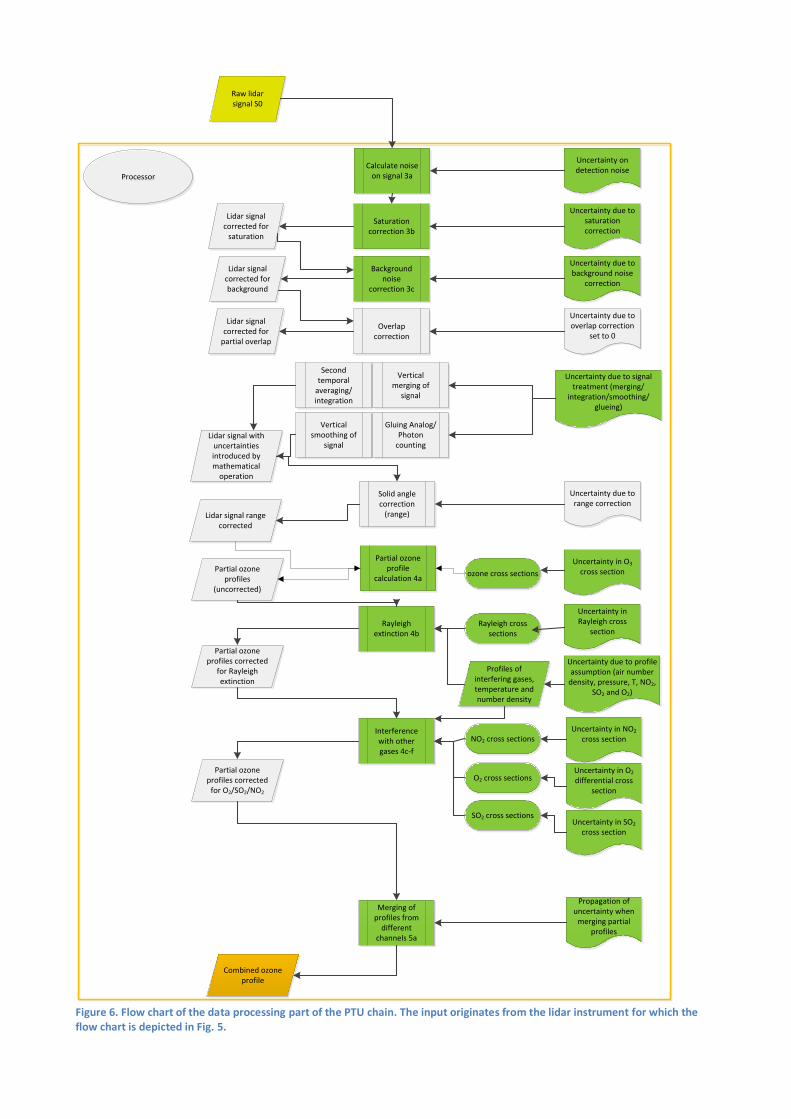
5 Product Traceability Chain The PTU is given below for ozone profile retrievals in the stratosphere and troposphere with DIAL.
The PTU is divided into two sections: the physical model is presented in Figure 5 and the
processing model in Figure 6. The numbered boxes in these figures indicate the key elements in the
PTU chain that are the main contributors to the overall measurement uncertainty. Each of these
elements is discussed in Section 6.
BackgroundSky illumination
straylight
Optics2a
Optics2a
Raw lidar signal S0
Dead-time
Emission subsystem1
Emission subsystem1
mediummedium
Receiver subsystem2
Receiver subsystem2
Interfering gases
Uncertainty due to interfering gases
Uncertainty due to contaminating light
Uncertainty due to imperfect/varying
alignmentDark current
Uncertainty due to saturation of
photon counters
Light scattering
Alignment2b
Absorption by other
molecules
Uncertainty due to dead time correction
Uncertainty due to Rayleigh extinction
Outgoing laser beam(s)
Figure 5. Four elements are shown in the physical part of the PTU chain: the emitter box (outlined by the green rectangle), the medium corresponding to the atmosphere (blue rectangle), the receiver box with e.g. the optics and detectors (yellow rectangle) and the processing software (orange rectangle on the following page). Processes and uncertainties that are considered in this document are shown as filled green shapes. Other sources of uncertainty have been listed, but are either, considered negligible, highly variable and therefore very hard to quantify, or avoidable (by proper technical design of the instrument).
Rayleigh extinction 4b
Second temporal
averaging/integration
Interference with other gases 4c-f
Vertical merging of
signal
Vertical smoothing of
signal
Overlap correction
Raw lidar signal S0
Background noise
correction 3c
Rayleigh cross sections
Solid angle correction
(range)
Gluing Analog/Photon
counting
ProcessorProcessor
Uncertainty due to overlap correction
set to 0
Uncertainty due to background noise
correction
Uncertainty due to signal treatment (merging/
integration/smoothing/glueing)
Uncertainty due to saturation correction
Uncertainty in Rayleigh cross
section
Uncertainty due to profile assumption (air number
density, pressure, T, NO2, SO2 and O2)
Propagation of uncertainty when
merging partial profiles
Lidar signal corrected for background
Lidar signal corrected for
partial overlap
Lidar signal with uncertainties introduced by mathematical
operation
Lidar signal range corrected
Merging of profiles from
different channels 5a
Uncertainty due to range correction
Saturation correction 3b
Lidar signal corrected for
saturation
Calculate noise on signal 3a
Partial ozone profiles corrected
for Rayleigh extinction
Partial ozone profiles corrected
for O2/SO2/NO2
Combined ozone profile
Profiles of interfering gases, temperature and number density
Uncertainty on detection noise
Uncertainty in O2 differential cross
section
Uncertainty in NO2 cross section
Uncertainty in O3 cross sectionozone cross sections
NO2 cross sections
SO2 cross sections
O2 cross sections
Uncertainty in SO2 cross section
Partial ozone profiles
(uncorrected)
Partial ozone profile
calculation 4a
Figure 6. Flow chart of the data processing part of the PTU chain. The input originates from the lidar instrument for which the flow chart is depicted in Fig. 5.
6 Element contributions
Emission sub-system (1) Light pulses at wavelengths 𝜆𝐿 = 308 and 353/355 nm for stratospheric ozone DIAL and 266, 277,
287, 289, 291, 299, 313 and/or 316 nm for tropospheric ozone are sent out into the atmosphere by a
laser transmitter directly or by means of transmission optics (mirrors, beam expander, etc.), and, if
necessary, after Raman shifting to obtain another wavelength than the one produced by the laser.
The parameters of the laser transmitter (pulse duration, energy and repetition rate, beam diameter
and divergence) as well as of the transmission optics change are distinct for each lidar system. For
this PTU, the distinction is that the stratospheric DIAL systems use larger telescopes (in the order of
1 m diameter) (McDermid, 1995), while the tropospheric lidars has a telescope with a diameter of
about 90 cm and has several additional small receivers to cover the lowest ranges (McDermid,
2002). Changes over time due to aging and replacement of components, as well as responses to
temperature changes may cause these parameters to change. These variations affect the optical
power transmitted into the atmosphere.
Information / data Type / value / equation Notes / description
Name of effect Transmission system
Contribution of variations in
all the parameters related to
the laser beam transmission to
the atmosphere.
Contribution identifier 1
Measurement equation
parameter(s) subject to effect
𝑃𝐿 and ξ(λON, λOFF) in lidar
equation
Contribution subject to effect
(final product or sub-tree
intermediate product)
Lidar signal
Time correlation extent & form Various time scales Extent & form not quantified
Other (non-time) correlation
extent & form
1) Possible correlation with
vertical range (if pulse
duration increases so as to
exceed the dwell time);
2) Possible correlation with
the temperature of laser and
transmission optics during
measurements
Extent & form not quantified
Uncertainty PDF shape N/A Systematic effect
Uncertainty & units 0% (relative uncertainty) (Assumed to be negligible)
Sensitivity coefficient < 1 (Assumed to be negligible)
Correlation(s) between affected
parameters None
Element/step common for all
sites/users? Yes
Traceable to ... N/A
Validation N/A
Receiving sub-system (2) The portion of the laser radiation backscattered by the atmosphere at different altitude ranges is
collected by a telescope. For tropospheric ozone DIAL the best suitable wavelengths to be used are
below 300 nm. For stratospheric ozone DIAL, wavelengths longer than 300 nm are used. Two or
more telescopes with different collecting apertures are usually employed to optimally cover the
signal dynamic range (near range, far range). The radiation collected by the telescope passes
through an optical system (consisting of lenses, mirrors, filters, beam splitters and interference
filters) where it is spectrally filtered, so only backscattered light at the ON and OFF wavelengths
are transmitted to the detection system. The uncertainty contribution of the receiving system is the
combination of contributions related to the receiver optical parameters (2a) and the alignment of the
lidar system (2b), whose uncertainties and correlation effects are described in the corresponding
sub-level sections.
Information / data Type / value / equation Notes / description
Name of effect Receiving system
Combined contribution of the receiver optical parameters
(2a) and alignment of the lidar system (2b)
Contribution identifier 2
Measurement equation parameter(s)
subject to effect
ξ(λL, λS) in lidar
equation
Contribution subject to effect (final
product or sub-tree intermediate
product)
Ozone profile NO3(z)
Time correlation extent & form Various time scales Extent & form not quantified
Other (non-time) correlation extent
& form
May affect vertical
correlation
Uncertainty PDF shape N/A Systematic effect
Uncertainty & units 0% (relative uncertainty)
combination of 2a and 2b Assumed to be negligible
Sensitivity coefficient 1
Correlation(s) between affected
parameters None
Element/step common for all
sites/users? Yes
Traceable to ... N/A
Validation N/A
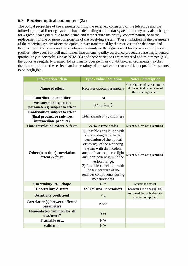
Receiver optical parameters (2a) The optical properties of the elements forming the receiver, consisting of the telescope and the
following optical filtering system, change depending on the lidar system, but they may also change
for a given lidar system due to their time and temperature instability, contamination, or to the
replacement of one or more components of the receiving system. These variations in the parameters
of the receiving system affect the optical power transmitted by the receiver to the detectors and
therefore both the power and the random uncertainty of the signals used for the retrieval of ozone
profiles. However, for well maintained instruments, quality assurance procedures are implemented
(particularly in networks such as NDACC) and these variations are monitored and minimized (e.g.,
the optics are regularly cleaned, lidars usually operate in air-conditioned environments), so that
their contribution to the retrieval and uncertainty of aerosol extinction coefficient profile is assumed
to be negligible.
Information / data Type / value / equation Notes / description
Name of effect
Receiver optical parameters
Contribution of variations in
all the optical parameters of
the receiving system
Contribution identifier 2a
Measurement equation
parameter(s) subject to effect ξ(λON, λOFF)
Contribution subject to effect
(final product or sub-tree
intermediate product)
Lidar signals PON and POFF
Time correlation extent & form Various time scales Extent & form not quantified
Other (non-time) correlation
extent & form
1) Possible correlation with
vertical range due to the
correlation of the optical
efficiency of the receiving
system with the incident
angle of backscattered light
and, consequently, with the
vertical range;
2) Possible correlation with
the temperature of the
receiver components during
measurements
Extent & form not quantified
Uncertainty PDF shape N/A Systematic effect
Uncertainty & units 0% (relative uncertainty) (Assumed to be negligible)
Sensitivity coefficient < 1 Assumed that only data not
effected is reported
Correlation(s) between affected
parameters None
Element/step common for all
sites/users? Yes
Traceable to ... N/A
Validation N/A
Alignment (2b) The correct alignment of the lidar system, that is the alignment of the laser beam with the receiving
system and of the telescope with the optics of filtering system, is ensured by specific tests, as for
instance developed in the frame of EARLINET quality assurance program. In particular, the so-
called telecover test and the Rayleigh fit test are performed to check and correct the alignment of
the lidar system in the near range (planetary bondary layer) and in the far range (free troposphere or
above), respectively – see Freudenthaler (AMTD, 2018).
For each lidar system there is a certain degree of misalignment between the laser beam and the
receiving system due to residual uncertainties in the telecover and Rayleigh fit tests or possible
mechanical/thermal instabilities of the optical and mechanical components forming both
transmission and receiving systems. The misalignment of a lidar system changes the angle on the
receiver of the backscattered light at each altitude level, which affects the overlap function. For the
DIAL application, there may be configurations that use multiple (two or more) outgoing laser
beams that have to be co-aligned with one or more receivers. This gives rise to multiple overlap
functions: one overlap function for earch laser beam and associated detetction channel. This implies
a minimum overlap height for each of these overlap fuctions. For the DIAL technique to be reliably
applied, only the data points originating from above the overlap function with the maximum overlap
range should be applied. For the application of the DIAL technique, technical provisions should be
in place to determine proper alignment, so that the minimum distance for data analysis can be
determined. The minimum distance amounts to less than 10 km for stratospheric ozone lidars and
less than 3 km for tropospheric ozone lidar.
Information / data Type / value / equation Notes / description
Name of effect Alignment
Contribution identifier 2b
Measurement equation
parameter(s) subject to effect ξ(λON,λOFF)
Contribution subject to effect
(final product or sub-tree
intermediate product)
Lidar signals PON and POFF
Time correlation extent & form Various time scales Extent & form not quantified
Other (non-time) correlation
extent & form
1) Possible correlation with
vertical range due to the
correlation of O(z) and
optical efficiency of the
receiving system with the
vertical range;
2) Possible correlation with
the temperature of
components forming both
transmission and receiving
systems during
measurements
Extent & form not quantified
Uncertainty PDF shape N/A Systematic effect
Uncertainty & units 0% (relative uncertainty) Assumed to be negligible
Sensitivity coefficient <1 Assumed that only data not
effected is reported
Correlation(s) between affected
parameters None
Element/step common for all
sites/users? Yes
Traceable to ... No
Validation No
Pre-processing (3)
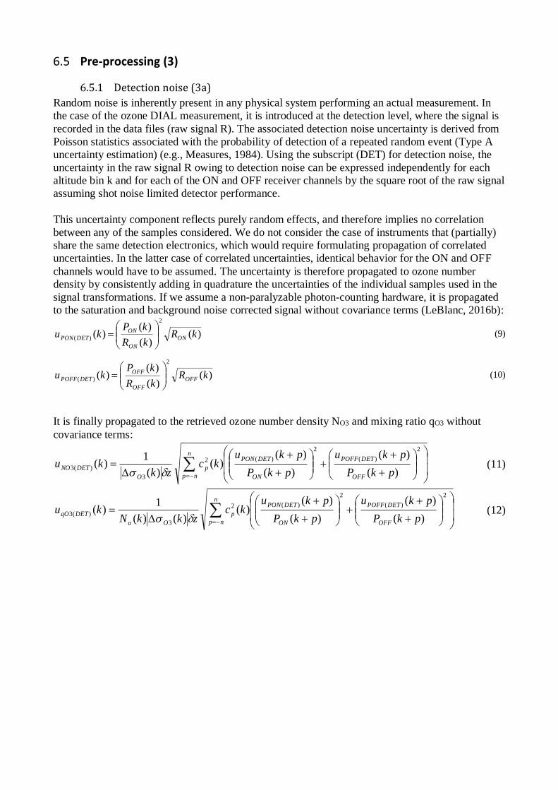
6.5.1 Detection noise (3a)
Random noise is inherently present in any physical system performing an actual measurement. In
the case of the ozone DIAL measurement, it is introduced at the detection level, where the signal is
recorded in the data files (raw signal R). The associated detection noise uncertainty is derived from
Poisson statistics associated with the probability of detection of a repeated random event (Type A
uncertainty estimation) (e.g., Measures, 1984). Using the subscript (DET) for detection noise, the
uncertainty in the raw signal R owing to detection noise can be expressed independently for each
altitude bin k and for each of the ON and OFF receiver channels by the square root of the raw signal
assuming shot noise limited detector performance.
This uncertainty component reflects purely random effects, and therefore implies no correlation
between any of the samples considered. We do not consider the case of instruments that (partially)
share the same detection electronics, which would require formulating propagation of correlated
uncertainties. In the latter case of correlated uncertainties, identical behavior for the ON and OFF
channels would have to be assumed. The uncertainty is therefore propagated to ozone number
density by consistently adding in quadrature the uncertainties of the individual samples used in the
signal transformations. If we assume a non-paralyzable photon-counting hardware, it is propagated
to the saturation and background noise corrected signal without covariance terms (LeBlanc, 2016b):
)()(
)()(
2
)( kRkR
kPku ON
ON
ON
DETPON
(9)
)()(
)()(
2
)( kRkR
kPku OFF
OFF
OFF
DETPOFF
(10)
It is finally propagated to the retrieved ozone number density NO3 and mixing ratio qO3 without
covariance terms:
n
np OFF
DETPOFF
ON
DETPON
p
O
DETNOpkP
pku
pkP
pkukc
zkku
2
)(
2
)(2
3
)(3)(
)(
)(
)()(
)(
1)(
(11)
n
np OFF
DETPOFF
ON
DETPON
p
Oa
DETqOpkP
pku
pkP
pkukc
zkkNku
2
)(
2
)(2
3
)(3)(
)(
)(
)()(
)()(
1)(
(12)
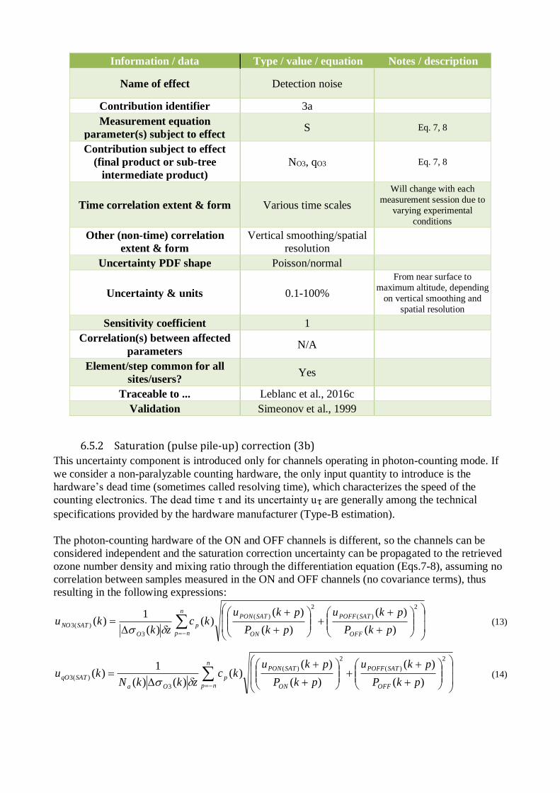
Information / data Type / value / equation Notes / description
Name of effect Detection noise
Contribution identifier 3a
Measurement equation
parameter(s) subject to effect S Eq. 7, 8
Contribution subject to effect
(final product or sub-tree
intermediate product)
NO3, qO3 Eq. 7, 8
Time correlation extent & form Various time scales
Will change with each
measurement session due to
varying experimental
conditions
Other (non-time) correlation
extent & form
Vertical smoothing/spatial
resolution
Uncertainty PDF shape Poisson/normal
Uncertainty & units 0.1-100%
From near surface to
maximum altitude, depending
on vertical smoothing and
spatial resolution
Sensitivity coefficient 1
Correlation(s) between affected
parameters N/A
Element/step common for all
sites/users? Yes
Traceable to ... Leblanc et al., 2016c
Validation Simeonov et al., 1999
6.5.2 Saturation (pulse pile-up) correction (3b)
This uncertainty component is introduced only for channels operating in photon-counting mode. If
we consider a non-paralyzable counting hardware, the only input quantity to introduce is the
hardware’s dead time (sometimes called resolving time), which characterizes the speed of the
counting electronics. The dead time τ and its uncertainty uτ are generally among the technical
specifications provided by the hardware manufacturer (Type-B estimation).
The photon-counting hardware of the ON and OFF channels is different, so the channels can be
considered independent and the saturation correction uncertainty can be propagated to the retrieved
ozone number density and mixing ratio through the differentiation equation (Eqs.7-8), assuming no
correlation between samples measured in the ON and OFF channels (no covariance terms), thus
resulting in the following expressions:
n
np OFF
SATPOFF
ON
SATPON
p
O
SATNOpkP
pku
pkP
pkukc
zkku
2
)(
2
)(
3
)(3)(
)(
)(
)()(
)(
1)(
(13)
n
np OFF
SATPOFF
ON
SATPON
p
Oa
SATqOpkP
pku
pkP
pkukc
zkkNku
2
)(
2
)(
3
)(3)(
)(
)(
)()(
)()(
1)(
(14)
Information / data Type / value / equation Notes / description
Name of effect Saturation correction
Contribution identifier 3b
Measurement equation
parameter(s) subject to effect S Eq. 7, 8
Contribution subject to effect
(final product or sub-tree
intermediate product)
NO3, qO3 Eq. 7, 8
Time correlation extent & form Various time scales
Will change with each
measurement session due to
varying experimental
conditions
Other (non-time) correlation
extent & form N/A
Uncertainty PDF shape Poisson/normal
Uncertainty & units
Tropospheric ozone: 20%
near the surface, nonlinearly
decreasing with altitude to
near 0, when switching to
other channel jumping to a
smaller peak, followed by
the nonlinear decrease with
altitude
For stratospheric ozone it
works similarly, except that
the maximum is about 1%
From near surface to
maximum altitude
Sensitivity coefficient 1
Correlation(s) between affected
parameters N/A
Element/step common for all
sites/users? Yes
Traceable to ... Leblanc et al., 2016c
Validation Donovan et al, 2003
Bristow, 1998
6.5.3 Background noise extraction (3c)
At far range (over 100 km range), the backscattered signal is too weak to be detected and any non-
zero signal reflects the presence of undesired skylight or electronic background noise. This noise is
typically subtracted from the total signal by fitting the uppermost part of the lidar signal with a
linear or non-linear function of altitude B. A new uncertainty component associated with the noise
fitting procedure must therefore be introduced. Here we provide a detailed treatment for the simple
case of a linear fit. It can be easily generalized to many other fitting functions. The linear fitting
function takes the form: )()( 10 kzbbkB (15)
For many well-known fitting methods (e.g., least-squares), the fitting coefficients bi can be
calculated analytically together with their uncertainty ubi and their correlation coefficient rbi,bj
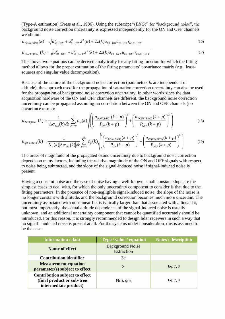
(Type-A estimation) (Press et al., 1986). Using the subscript “(BKG)” for “background noise”, the
background noise correction uncertainty is expressed independently for the ON and OFF channels
we obtain:
ONbbONbONbONbONbBKGPON ruukzkzuuku _1,0_1_0
22
_1
2
_0)( )(2)()( (16)
OFFbbOFFbOFFbOFFbOFFbBKGPOFF ruukzkzuuku _1,0_1_0
22
_1
2
_0)( )(2)()( (17)
The above two equations can be derived analytically for any fitting function for which the fitting
method allows for the proper estimation of the fitting parameters’ covariance matrix (e.g., least-
squares and singular value decomposition).
Because of the nature of the background noise correction (parameters bi are independent of
altitude), the approach used for the propagation of saturation correction uncertainty can also be used
for the propagation of background noise correction uncertainty. In other words since the data
acquisition hardware of the ON and OFF channels are different, the background noise correction
uncertainty can be propagated assuming no correlation between the ON and OFF channels (no
covariance terms):
n
np OFF
BKGPOFF
ON
BKGPON
p
O
BKGNOpkP
pku
pkP
pkukc
zkku
2
)(
2
)(
3
)(3)(
)(
)(
)()(
)(
1)(
(18)
n
np OFF
BKGPOFF
ON
BKGPON
p
Oa
BKGqOpkP
pku
pkP
pkukc
zkkNku
2
)(
2
)(
3
)(3)(
)(
)(
)()(
)()(
1)(
(19)
The order of magnitude of the propagated ozone uncertainty due to background noise correction
depends on many factors, including the relative magnitude of the ON and OFF signals with respect
to noise being subtracted, and the slope of the signal-induced noise if signal-induced noise is
present.
Having a constant noise and the case of noise having a well-known, small constant slope are the
simplest cases to deal with, for which the only uncertainty component to consider is that due to the
fitting parameters. In the presence of non-negligible signal-induced noise, the slope of the noise is
no longer constant with altitude, and the background correction becomes much more uncertain. The
uncertainty associated with non-linear fits is typically larger than that associated with a linear fit,
but most importantly, the actual altitude dependence of the signal-induced noise is usually
unknown, and an additional uncertainty component that cannot be quantified accurately should be
introduced. For this reason, it is strongly recommended to design lidar receivers in such a way that
no signal—induced noise is present at all. For the systems under consideration, this is assumed to
be the case.
Information / data Type / value / equation Notes / description
Name of effect Background Noise
Extraction
Contribution identifier 3c
Measurement equation
parameter(s) subject to effect S Eq. 7, 8
Contribution subject to effect
(final product or sub-tree
intermediate product)
NO3, qO3 Eq. 7, 8
Time correlation extent & form Various time scales
Another source of uncertainty introduced in Eq. (7) is the a priori use of ancillary NO2 and SO2
number density or mixing ratio profiles. The term “a priori” here does not mean that the ozone
DIAL retrieval uses a variational/optimal estimation method (it does not), but simply means that the
information comes from ancillary (i.e., non-lidar) measurements or models, and is input as “truth”
in the ozone DIAL processing chain. The input quantities in this case can be of a different nature,
namely mixing ratio or number density (e.g., Ahmad et al., 2007; Bauer et al., 2012; Bracher et al.,
2005; Brohede et al., 2007; Brühl et al., 2013; Cao et al., 2006; Hopfner et al., 2013; He et al., 2014;
McLinden et al., 2014). In order to ensure self-consistency in our measurement model, input
quantities independent of air number density should be chosen:
• When the input quantity independent of air number density is the interfering gas’ number
density Nig (with uncertainty uNig), the propagated ozone number density and mixing ratio
uncertainties should be written:
)()(
)()(
3
)(3 kuk
kku Nig
O
ig
NigNO
with ig = NO2, SO2 (50)
)()(
)(
)(
1)(
3
)(3 kuk
k
kNku Nig
O
ig
a
NigqO
with ig = NO2, SO2 (51)
• When the input quantity independent of air number density is the interfering gas’ mixing
ratio qig (with uncertainty uqig), the propagated ozone number density and mixing ratio
uncertainties should be written:
)()(
)()()(
3
)(3 kuk
kkNku qig
O
Nig
aqigNO
with ig = NO2, SO2 (52)
)()(
)()(
3
)(3 kuk
kku qig
O
Nig
qigqO
with ig = NO2, SO2 (53)
Equation (53) shows that the lidar-retrieved ozone mixing ratio uncertainty due to the interfering
gases is directly proportional to the gases’ mixing ratio uncertainty. The NO2 mixing ratio
uncertainty component remains very small in most cases. One exception is for highly-polluted
boundary layer conditions where NO2 mixing ratio can reach 10 to 100 ppbv, resulting in ozone
mixing ratio uncertainty of 0.5 to 5 ppbv for the most-commonly used DIAL wavelengths.
Tropospheric ozone DIAL pairs are more affected in polluted conditions case due to the larger SO2
absorption cross-section differential at the wavelengths used for tropospheric ozone DIAL.
Information / data Type / value / equation Notes / description
Name of effect Interfering gases’
atmospheric profiles
Contribution identifier 4e
Measurement equation
parameter(s) subject to effect 𝑁𝑖𝑔 , 𝑞𝑖𝑔 Eq. 7, 8
Contribution subject to effect
(final product or sub-tree
intermediate product)
NO3, qO3 Eq. 7, 8
Time correlation extent & form Various time scales
Will change with each
measurement session due to
varying experimental
conditions in terms of
atmospheric composition
Other (non-time) correlation
extent & form None
Uncertainty PDF shape Poisson/normal
Uncertainty & units
NO2: 0.01-10% tropospheric
DIAL
0.001-0.1%
stratospheric DIAL
SO2: 0.01-100%
tropospheric DIAL
0.001-0.1%
stratospheric DIAL
Uncertainty depends on
wavelengths used for the
measurement (tropospheric or
stratospheric DIAL)
Sensitivity coefficient 1
Correlation(s) between affected
parameters None
Element/step common for all
sites/users? Yes
Traceable to ... Leblanc et al., 2016c
Validation None
6.6.6 Uncertainty owing to air number density, temperature and pressure profiles (4f)
The last input quantity to consider in our ozone DIAL measurement model is ancillary air number
density. Air density is generally not estimated directly, but rather derived from air temperature and
pressure. Here we provide expressions for the propagation of this uncertainty component for both
cases, i.e., when air number density is considered the input quantity, and when temperature and
pressure are considered the input quantities.
6.6.6.1 Estimation from air number density profile If the air number density Na is not derived from air temperature and pressure, then its uncertainty
uNa can be propagated directly to ozone number density and mixing ratio. The result however will
be different whether mixing ratio or number density is used as input quantity for the interfering
gases’ profiles:
• If number density is used as input quantity for the interfering gases’ profiles:
)()(
)()(
3
22
)(3 kuk
kqku Na
O
OOM
NaNO
(54)
)(
)(
)(
)()(
3
22
3)(3kN
ku
k
kqqku
a
Na
O
OOM
ONaqO
(55)
• If mixing ratio is used as input quantity for the interfering gases’ profiles:
)()(
)()()()()()(
3
222222
)(3 kuk
kqkqkkqkku Na
O
OOSOSONONOM
NaNO
(56)
)(
)(
)(
)()()()()()(
3
222222
3)(3kN
ku
k
kqkqkkqkqku
a
Na
O
OOSOSONONOM
ONaqO
(57)
In Eqs. (54)-(57), the effect of absorption by O2 in the Herzberg and Wulf bands region is included.
This term can be neglected if the ON and OFF wavelengths are longer than 294 nm. In Eq. (57), it
is again assumed that the interfering gases’ mixing ratio profiles are independent from the air
number density profile (no covariance terms involved).
6.6.6.2 Estimation from air temperature and pressure profile When using radiosonde measurements, meteorological analysis, or assimilation models, the air
number density is typically derived from air temperature Ta and pressure pa following the ideal gas
law (with kB being the Boltzmann constant):
)(
)()(
kTk
kpkN
aB
a
a (58)
In this case, air number density is no longer the input quantity, but air temperature and pressure are.
The propagation of uncertainty due to the use of an a priori temperature and pressure profile now
depends on the degree of correlation between pressure and temperature.
• If temperature and pressure are measured or computed independently, with uncertainty
estimates uTa and upa respectively, and if number density is used as input quantity for the
interfering gases, the air number density uncertainty propagated to ozone number density
and mixing ratio will be:
)(
)(
)(
)()(
)(
)()(
2
2
2
2
3
22
)(3kT
ku
kp
kukN
k
kqku
a
Ta
a
pa
a
O
OOM
NaNO
(59)
)(
)(
)(
)(
)(
)()(
2
2
2
2
3
22
)(3kT
ku
kp
ku
k
kqku
a
Ta
a
pa
O
OOM
NaqO
(60)
• If temperature and pressure are measured or computed independently, with uncertainty
estimates uTa and upa respectively, and if mixing ratio is used as input quantity for the
interfering gases, the air number density uncertainty propagated to ozone number density
will be:
)(
)(
)(
)()(
)(
)()()()(
2
2
2
2
3
222222
)(3kT
ku
kp
kukN
k
kqkqkqku
a
Ta
a
pa
a
O
OOSOSONONOM
NaNO
(61)
• If temperature and pressure are known to be fully correlated, and if number density is used
as input quantity for the interfering gases, the ozone number density uncertainty due to air
number density will be written:
)(
)(
)(
)()(
)(
)()(
3
22
)(3kT
ku
kp
kukN
k
kqku
a
Ta
a
pa
a
O
OOM
NaNO
(62)
• If temperature and pressure are known to be fully correlated, and if mixing ratio is used as
input quantity for the interfering gases, the ozone number density uncertainty due to air
number density will be written:
)(
)(
)(
)()(
)(
)()()()(
3
222222
)(3kT
ku
kp
kukN
k
kqkqkqku
a
Ta
a
pa
a
O
OOSOSONONOM
NaNO
(63)
Because the ozone and interfering gases’ absorption cross-sections depend on temperature, the
covariance terms of the cross-section differentials and the air number density covariance matrix are
not strictly zero. However the correlation coefficients are expected to be very small and the
assumption of two “independent” input quantities still holds.
The largest ozone uncertainty in the upper stratosphere is that due to pressure. DIAL pairs using
longer wavelengths (e.g., 299/316 nm) are more impacted than pairs using shorter wavelengths, in
particular the tropospheric ozone DIAL. Note that with current pressure-temperature measurement
capabilities (typically 0.5 K and 0.1 hPa uncertainties), the lidar-retrieved ozone uncertainty due to
temperature is about 10 times larger than that due to pressure uncertainty.
Information / data Type / value / equation Notes / description
Name of effect
External air number density,
temperature and pressure
profiles
This table corresponds to both
6.6.6.1 and 6.6.6.2
Contribution identifier 4f
Measurement equation
parameter(s) subject to effect 𝑁𝑎 Eq. 7
Contribution subject to effect
(final product or sub-tree
intermediate product)
NO3, qO3 Eq. 7, 8
Time correlation extent & form Various time scales
Will change with each
measurement session due to
varying experimental
conditions in terms of
atmospheric state
Other (non-time) correlation
extent & form None
Uncertainty PDF shape Poisson/normal
Uncertainty & units
<1% for stratospheric ozone,
<0.1% for tropospheric
ozone. When using VMR,
the uncertainty associated
with this item can be
substantial; linked to the
uncertainty of the source
information
Sensitivity coefficient 1
Correlation(s) between affected
parameters None
Element/step common for all
sites/users? Yes
Traceable to ... Leblanc et al., 2016c
Validation
Godin-Beekmann et al.,
2003
Brinksma et al., 2000
Spatiotemporal integration (5)
6.7.1 Propagation of uncertainty when combining two intensity ranges (5a)
Ozone DIAL instruments are most often designed with multiple signal intensity ranges in order to
maximize the overall altitude range of the profile. Reduced signal intensity is achieved using neutral
density filters or other optical systems attenuating the Rayleigh-backscattered signals, or using
Raman backscatter channels which typically are 750 times weaker than Rayleigh backscatter
channels. Until now, our ozone DIAL measurement model referred to a single intensity range. We
now provide a formulation for the propagation of uncertainty when at least two intensity ranges are
combined to form a single profile. Combining individual intensity ranges into a single profile can
occur either during lidar signal processing or after the ozone number density is calculated
individually for each intensity range. Here we present the case of combining ozone number density
after it was calculated for individual intensity ranges. The case of combining the lidar signals is
presented in Leblanc et al., 2016a and is applied in the selected cases for GaiaClim. The principles
governing the propagation of uncertainty are the same in both cases.
A single profile covering the entire useful range of the instrument is typically obtained by
combining the most accurate overlapping sections of the profiles retrieved from individual ranges.
The thickness of the transition region typically varies from a few meters to a few kilometres,
depending on the instrument and on the intensity ranges considered. Assuming that the transition
region’s bottom altitude is z(k1) and its top altitude is z(k2), the combined ozone profile between a
low range iL and a high range iH, is typically obtained by computing a weighted average of the
ozone values retrieved for each range:
),()(1),()()( 333 HOLOO ikNkwikNkwkN k1 < k < k2 and 0 < w(k) < 1 (64)
),()(1),()()( 333 HOLOO ikqkwikqkwkq k1 < k < k2 and 0 < w(k) < 1 (65)
Using this formulation, all uncertainty components associated with atmospheric extinction
corrections are propagated without change as they do not depend on the intensity range considered:
),(),()( )(3)(3)(3 HXNOLXNOXNO ikuikuku for all k (66)
),(),()( )(3)(3)(3 HXqOLXqOXqO ikuikuku for all k (67)
With X = O3, M, Na, ig, Nig, O2 and ig = NO2, SO2.
Because of its random nature, ozone uncertainty due to detection noise for the combined profile is
obtained by adding in quadrature (no covariance terms) the detection noise uncertainties of the
individual ranges:
2)(3
2
)(3)(3 ),()(1),()()( HDETNOLDETNODETNO ikukwikukwku k1 < k < k2 (68)
2)(3
2
)(3)(3 ),()(1),()()( HDETqOLDETqODETqO ikukwikukwku k1 < k < k2 (69)
Assuming that the saturation correction and the background noise extraction have been applied
consistently for all intensity ranges within the same data processing algorithm, the associated
uncertainty components can be propagated to the combined profile assuming full correlation
between the intensity ranges:
),()(1),()()( )(3)(3)(3 HXNOLXNOXNO ikukwikukwku k1 < k < k2 (70)
),()(1),()()( )(3)(3)(3 HXqOLXqOXqO ikukwikukwku k1 < k < k2 (71)
with X = SAT, BKG.
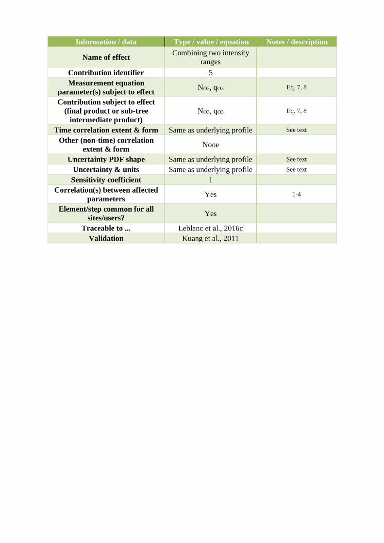
Information / data Type / value / equation Notes / description
Name of effect Combining two intensity
ranges
Contribution identifier 5
Measurement equation
parameter(s) subject to effect NO3, qO3 Eq. 7, 8
Contribution subject to effect
(final product or sub-tree
intermediate product)
NO3, qO3 Eq. 7, 8
Time correlation extent & form Same as underlying profile See text
Other (non-time) correlation
extent & form None
Uncertainty PDF shape Same as underlying profile See text
Uncertainty & units Same as underlying profile See text
Sensitivity coefficient 1
Correlation(s) between affected
parameters Yes 1-4
Element/step common for all
sites/users? Yes
Traceable to ... Leblanc et al., 2016c
Validation Kuang et al., 2011
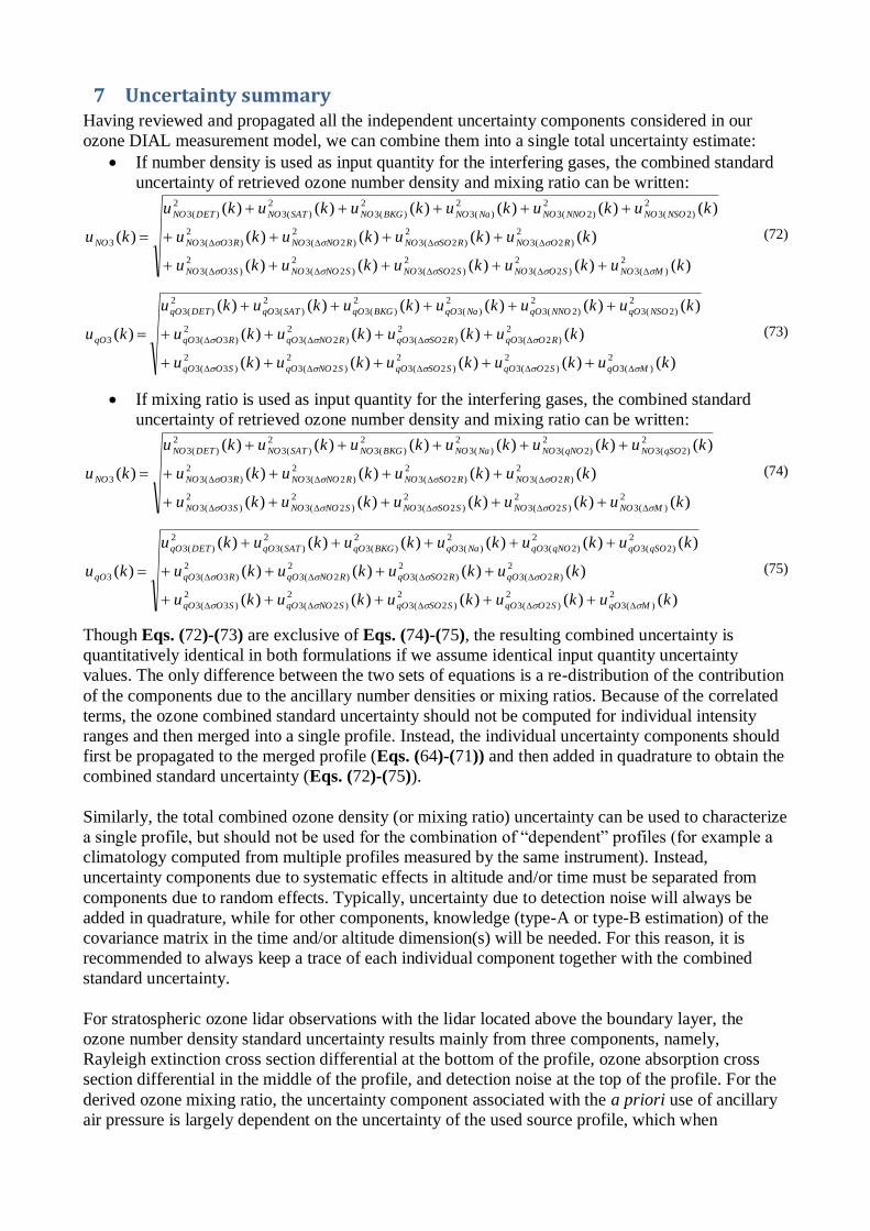
7 Uncertainty summary Having reviewed and propagated all the independent uncertainty components considered in our
ozone DIAL measurement model, we can combine them into a single total uncertainty estimate:
• If number density is used as input quantity for the interfering gases, the combined standard
uncertainty of retrieved ozone number density and mixing ratio can be written:
)()()()()(
)()()()(
)()()()()()(
)(
2
)(3
2
)2(3
2
)2(3
2
)2(3
2
)3(3
2
)2(3
2
)2(3
2
)2(3
2
)3(3
2
)2(3
2
)2(3
2
)(3
2
)(3
2
)(3
2
)(3
3
kukukukuku
kukukuku
kukukukukuku
ku
MNOSONOSSONOSNONOSONO
RONORSONORNONORONO
NSONONNONONaNOBKGNOSATNODETNO
NO
(72)
)()()()()(
)()()()(
)()()()()()(
)(
2
)(3
2
)2(3
2
)2(3
2
)2(3
2
)3(3
2
)2(3
2
)2(3
2
)2(3
2
)3(3
2
)2(3
2
)2(3
2
)(3
2
)(3
2
)(3
2
)(3
3
kukukukuku
kukukuku
kukukukukuku
ku
MqOSOqOSSOqOSNOqOSOqO
ROqORSOqORNOqOROqO
NSOqONNOqONaqOBKGqOSATqODETqO
qO
(73)
• If mixing ratio is used as input quantity for the interfering gases, the combined standard
uncertainty of retrieved ozone number density and mixing ratio can be written:
)()()()()(
)()()()(
)()()()()()(
)(
2
)(3
2
)2(3
2
)2(3
2
)2(3
2
)3(3
2
)2(3
2
)2(3
2
)2(3
2
)3(3
2
)2(3
2
)2(3
2
)(3
2
)(3
2
)(3
2
)(3
3
kukukukuku
kukukuku
kukukukukuku
ku
MNOSONOSSONOSNONOSONO
RONORSONORNONORONO
qSONOqNONONaNOBKGNOSATNODETNO
NO
(74)
)()()()()(
)()()()(
)()()()()()(
)(
2
)(3
2
)2(3
2
)2(3
2
)2(3
2
)3(3
2
)2(3
2
)2(3
2
)2(3
2
)3(3
2
)2(3
2
)2(3
2
)(3
2
)(3
2
)(3
2
)(3
3
kukukukuku
kukukuku
kukukukukuku
ku
MqOSOqOSSOqOSNOqOSOqO
ROqORSOqORNOqOROqO
qSOqOqNOqONaqOBKGqOSATqODETqO
qO
(75)
Though Eqs. (72)-(73) are exclusive of Eqs. (74)-(75), the resulting combined uncertainty is
quantitatively identical in both formulations if we assume identical input quantity uncertainty
values. The only difference between the two sets of equations is a re-distribution of the contribution
of the components due to the ancillary number densities or mixing ratios. Because of the correlated
terms, the ozone combined standard uncertainty should not be computed for individual intensity
ranges and then merged into a single profile. Instead, the individual uncertainty components should
first be propagated to the merged profile (Eqs. (64)-(71)) and then added in quadrature to obtain the
combined standard uncertainty (Eqs. (72)-(75)).
Similarly, the total combined ozone density (or mixing ratio) uncertainty can be used to characterize
a single profile, but should not be used for the combination of “dependent” profiles (for example a
climatology computed from multiple profiles measured by the same instrument). Instead,
uncertainty components due to systematic effects in altitude and/or time must be separated from
components due to random effects. Typically, uncertainty due to detection noise will always be
added in quadrature, while for other components, knowledge (type-A or type-B estimation) of the
covariance matrix in the time and/or altitude dimension(s) will be needed. For this reason, it is
recommended to always keep a trace of each individual component together with the combined
standard uncertainty.
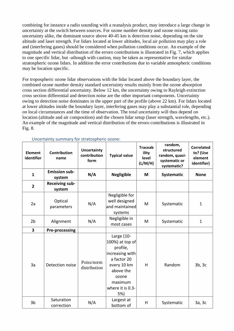
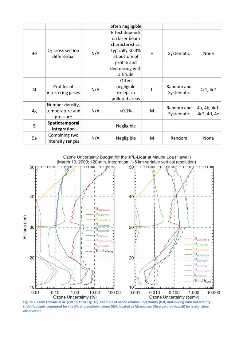
For stratospheric ozone lidar observations with the lidar located above the boundary layer, the
ozone number density standard uncertainty results mainly from three components, namely,
Rayleigh extinction cross section differential at the bottom of the profile, ozone absorption cross
section differential in the middle of the profile, and detection noise at the top of the profile. For the
derived ozone mixing ratio, the uncertainty component associated with the a priori use of ancillary
air pressure is largely dependent on the uncertainty of the used source profile, which when
combining for instance a radio sounding with a reanalysis product, may introduce a large change in
uncertainty at the switch between sources. For ozone number density and ozone mixing ratio
uncertainty alike, the dominant source above 40-45 km is detection noise, depending on the site
altitude and laser strength. For lidars located at lower altitudes, local air pollution may play a role
and (interfering gases) should be considered when pollution conditions occur. An example of the
magnitude and vertical distribution of the erroro contributions is illustrated in Fig. 7, which applies
to one specific lidar, but -athough with caution, may be taken as representative for similar
stratospheric ozone lidars. In addition the error contributions due to variable atmospheric conditions
may be location specific.
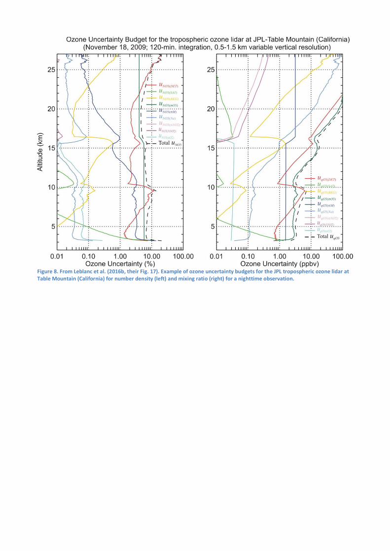
For tropospheric ozone lidar observations with the lidar located above the boundary layer, the
combined ozone number density standard uncertainty results mainly from the ozone absorption
cross section differential uncertainty. Below 12 km, the uncertainty owing to Rayleigh extinction
cross section differential and detection noise are the other important components. Uncertainty
owing to detection noise dominates in the upper part of the profile (above 22 km). For lidars located
at lower altitudes inside the boundary layer, interfering gases may play a substantial role, depending
on local circumstances and the time of observation. The total uncertainty will thus depend on
location (altitude and air composition) and the chosen lidar setup (laser strength, wavelengths, etc.).
An example of the magnitude and vertical distribution of the erroro contributions is illustrated in
Fig. 8.
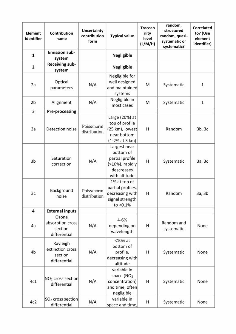
Uncertainty summary for stratospheric ozone:
Element identifier
Contribution name
Uncertainty contribution
form Typical value
Traceability level
(L/M/H)
random, structured
random, quasi-systematic or systematic?
Correlated to? (Use element
identifier)
1 Emission sub-
system N/A Negligible M Systematic None
2 Receiving sub-
system
2a Optical
parameters N/A
Negligible for well designed
and maintained systems
M Systematic 1
2b Alignment N/A Negligible in most cases
M Systematic 1
3 Pre-processing
3a Detection noise Poiss/norm
distribution
Large (10-100%) at top of
profile, increasing with
a factor 20 every 10 km
above the ozone
maximum where it is 0.3-
5%)
H Random 3b, 3c
3b Saturation correction
N/A Largest at bottom of
H Systematic 3a, 3c
partial profile (~1%), rapidly
decreasing with altitude
3c Background
noise Poiss/norm
distribution
1% near top of profile,
negligible 12 km below
H Random 3a, 3b
4 External inputs
4a
Ozone absorption cross
section differential
N/A 2% H Random and systematic
None
4b
Rayleigh extinction cross
section differential
N/A
Largest in lower part of
profile (<10%), below 1%
above 20 km
H Systematic None
4c1 NO2 cross section
differential N/A
Variable in space and time, often negligible
H Systematic None
4c2 SO2 cross section
differential N/A
Variable in space and time, often negligible
H Systematic None
4d O2 cross section
differential N/A
0 (only affects wavelength shorter than
294 nm)
H Systematic None
4e Profiles of
interfering gases N/A
Often negligible
except in highly polluted areas
L Random and Systematic
4c1, 4c2
4f Number density, temperature and
pressure N/A
<1% for ozone in number
density, large contribution in
mixing ratio, depending on uncertainty of
source
M Random and Systematic
4a, 4b, 4c1, 4c2, 4d, 4e
5 Spatiotemporal
integration
5a Combining two intensity ranges
N/A Negligible M Random None
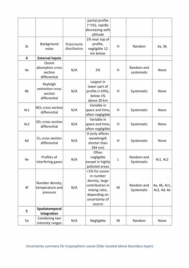
Uncertainty summary for tropospheric ozone (lidar located above boundary layer):
Element identifier
Contribution name
Uncertainty contribution
form Typical value
Traceability level
(L/M/H)
random, structured
random, quasi-systematic or systematic?
Correlated to? (Use element
identifier)
1 Emission sub-
system Negligible
2 Receiving sub-
system Negligible
2a Optical
parameters N/A
Negligible for well designed
and maintained systems
M Systematic 1
2b Alignment N/A Negligible in most cases
M Systematic 1
3 Pre-processing
3a Detection noise Poiss/norm
distribution
Large (20%) at top of profile
(25 km), lowest near bottom
(1-2% at 3 km)
H Random 3b, 3c
3b Saturation correction
N/A
Largest near bottom of
partial profile (>10%), rapidly
descreases with altitude
H Systematic 3a, 3c
3c Background
noise Poiss/norm
distribution
1% at top of partial profiles, decreasing with signal strength
to <0.1%
H Random 3a, 3b
4 External inputs
4a
Ozone absorption cross
section differential
N/A 4-6%
depending on wavelength
H Random and systematic
None
4b
Rayleigh extinction cross
section differential
N/A
<10% at bottom of
profile, decreasing with
altitude
H Systematic None
4c1 NO2 cross section
differential N/A
variable in space (NO2
concentration) and time, often
negligible
H Systematic None
4c2 SO2 cross section
differential N/A
variable in space and time,
H Systematic None
often negligible
4e O2 cross section
differential N/A
Effect depends on laser beam characteristics, typically <0.3%
at bottom of profile and
decreasing with altitude
H Systematic None
4f Profiles of
interfering gases N/A
Often negligible except in
polluted areas
L Random and Systematic
4c1, 4c2
4g Number density, temperature and
pressure N/A <0.1% M
Random and Systematic
4a, 4b, 4c1, 4c2, 4d, 4e
5 Spatiotemporal
integration Negligible
5a Combining two intensity ranges
N/A Negligible M Random None
Figure 7. From Leblanc et al. (2016b, their Fig. 16). Example of ozone relative uncertainty (left) and mixing ratio uncertainty (right) budgets computed for the JPL stratospheric ozone DIAL located at Mauna Loa Observatory (Hawaii) for a nighttime observation.
Figure 8. From Leblanc et al. (2016b, their Fig. 17). Example of ozone uncertainty budgets for the JPL tropospheric ozone lidar at Table Mountain (California) for number density (left) and mixing ratio (right) for a nighttime observation.
8 Traceability uncertainty analysis
Traceability level definition is given in Table 2.
Table 2. Traceability level definition table
Traceability Level Descriptor Multiplier
High SI traceable or globally
recognised community standard 1
Medium
Developmental community
standard or peer-reviewed
uncertainty assessment
3
Low Approximate estimation
10
Analysis of the uncertainty summaries would suggest the following contributions, shown in Table
3, should be considered further to improve the overall uncertainty of the DIAL ozone profile
product. The entires are given in an estimated priority order.
Table 3. Traceability level definition further action table.
Element identifier
Contribution name
Uncertainty contribution
form Typical value
Traceability level
(L/M/H)
random, structured
random, quasi-systematic or systematic?
Correlated to? (Use element
identifier)
4f Profiles of
interfering gases N/A
Often negligible except in
polluted areas
L Random and Systematic
4c1, 4c2
4g Number density, temperature and
pressure N/A <0.1% M
Random and Systematic
4a, 4b, 4c1, 4c2, 4d, 4e
Recommendations
For the benefit of increasing the usability of ozone profile data originating from Differential
Absorption Lidar instruments the recommendations are:
1. Application of the uncertainty propagation as outlined above and in more detailed form in
Leblanc et al. (2016b, 2016c) is recommended for all ozone lidar systems, in particular those
linked up in networks.
2. It should be technically feasible to set-up and operate a centralised data processing facility
for ozone lidar data, which would have the obvious benefit of homogeneous data processing
and therefore uncertainty budget estimation
3. Various variable uncertainty sources have been identified that are hard to quantify or highly
variable in space/time or instrument-specific. These are listed as uncertainty boxes that are
not filled green in Figures 8 and 9 which are expansions of those in section 5 (Figures 5 and
6). Further research into these items, and consideration of these items for individual systems
when determining their PTU, is recommended.
4. In the current uncertainty analysis, use of only photon counting is assumed. It is
recommended to include analysis for analog detection as well as the hybrid analog and
photon counting detection modes. This may be of particular interest for the application for
tropospheric ozone DIAL.
BackgroundSky illumination
straylight
OpticsOptics
digitizing
Uncertainty due to transmission and
timing issues
Raw lidar signal
Temporal averaging/integration
Dead-time
Spatial nonuniformity of the photomultiplier
photocathodes
Electromagnetically induced interference (in detection
subsystem placed in transmitter/receiver block)
Uneven aging of photomultipliers
Emission subsystem1
Emission subsystem1
mediummedium
Receiver subsystemReceiver subsystem
Interfering gases
Interfering liquids/solids
aerosols
Uncertainty due to interfering gases
Uncertainty due to aerosols
Uncertainty due to contaminating light
Uncertainty due to clouds
Uncertainty due to imperfect/varying
alignment
Uncertainty due to signal treatment
Uncertainty due to signal interference
Uncertainty due to trends in sensitivity of photoresponsive
material
Uncertainty due to instability of
discriminator cut-off levels
Dark current
Uncertainty due to spatiotemporal
variations in photomultiplier
response
Uncertainty due to saturation of
photon counters
Uncertainty due to multiple scattering
Light scattering
Alignment
Absorption by other
molecules
Uncertainty due to dead time correction
Uncertainty due to Rayleigh extinction
Uncertainty due to analog-to-digital
conversion
Figure 9. Expansion of flow chart in Fig. 5. Various variable uncertainty sources have been identified that are hard to quantify or highly variable in space/time or instrument-specific. These are listed as uncertainty boxes that are not filled green in the flowchart below which is an expansion of the one in section 5.
Rayleigh extinction
Second temporal
averaging/integration
Interference with other
gases
Vertical merging of
signal
Vertical smoothing of
signal
Collocation with external
data
Grid resolution
Spatial offset
Temporal offset
Overlap correction
Uncertainty of external source
Raw lidar signal
Background noise
correction
Coefficients fitting
Rayleigh cross sections
Solid angle correction
(range)
Gluing Analog/Photon
counting
ProcessorProcessor
Uncertainty due to overlap correction
Uncertainty due to background noise
correction
Uncertainty due to signal treatment (merging/
integration/smoothing/glueing)
Uncertainty due to saturation correction
Uncertainty in Rayleigh cross
section
Uncertainty due to profile assumption (air number
density, pressure, T)
Uncertainty due to collocation
Propagated uncertainties when
merging profiles
Uncertainty due to assumptions on
aerosol properties
Lidar signal corrected for background
Lidar signal corrected for
partial overlap
Lidar signal with uncertainties introduced by mathematical
operation
Lidar signal range corrected
Aerosol extinctioncorrection
Merging of profiles from
different channels
Uncertainty due to range correction
Saturation correction
Lidar signal corrected for
saturation
Calculate noise on signal
Partial ozone profiles corrected
for Rayleigh extinction
Partial ozone profile corrected for O2/SO2/NO2
Lidar signal corrected for
aerosol extinction
Temperature data
Profiles of interfering
gases
Aerosol profile data or
extinction measurements
Uncertainty due to temperature-
dependence of cross-sections
Uncertainty on detection noise
Multiple scattering correction
Uncertainty in O2 cross section
Uncertainty in NO2 cross section
Uncertainty in O3 cross section
ozone cross sections
NO2 cross sections
SO2 cross sections
O2 cross sections
Partial ozone profile
calculation
Uncertainty in SO2 cross section
Number density of pressure profile
Uncertainty due to profile assumption (SO2, NO2 and
O2)
Combined ozone profile
Partial ozone profiles
Lidar signal corrected for
multiple scattering
Uncertainty due to multiple scattering
correction
Figure 10. Expansion of flow chart in Fig. 6. Various variable uncertainty sources have been identified that are hard to quantify or highly variable in space/time or instrument-specific. These are listed as uncertainty boxes that are not filled green in the flowchart below which is an expansion of the one in section 5.
9 Conclusion The ozone profile differential absorption lidar product has been assessed against the GAIA CLIM
traceability and uncertainty criteria.
References 1. Ahmad, Z., McClain, C. R., Herman, J. R., Franz, B. A., Kwiatkowska, E. J., Robinson, W.
D., Bucsela, E. J., and Tzortziou, M.: Atmospheric correction for NO2 absorption in
retrieving water-leaving reflectances from the SeaWiFS and MODIS measurements, Appl.
Opt., 46(26), 6504-6512, 2007.
2. Bass, A. M., and Paur, R. J.: The Ultraviolet Cross-sections of Ozone: I. The Measurements,
Proc. Quadriennial Ozone Symp., Halkidiki, Greece, 606-616, 1984.
3. Bates, D. R.: Rayleigh-scattering by air, Planet Space Sci., 32, 785-790, 10.1016/0032-
0633(84)90102-8, 1984.
4. Bauer, R., Rozanov, A., McLinden, C. A., Gordley, L. L., Lotz, W., Russell, J. M., Walker,
K. A., Zawodny, J. M., Ladstatter-Weissenmayer, A., Bovensmann, H., and Burrows, J. P.:
Validation of SCIAMACHY limb NO2 profiles using solar occultation measurements,