Gains from Trade and Environmental Policy underImperfect Competition and Pollution from Transport 1

Luc Soete and Thomas Ziesemer

1. Introduction

The relationship between the environment and international trade has been investigated in the

framework of several international trade models that have been extended to contain the factor

environmental pollution. The Ricardian trade model has been used by Pethig (1976) and the

Heckscher-Ohlin model has been used in different ways by Pethig (1976), McGuire (1982)

and Merrifield (1988). Conrad (1993) applied the Cournot-Brander-Spencer model and

Markusen, Morey and Olewiler (1993) have applied the Horstmann-Markusen model. In this

paper we apply the Chamberlin-Krugman model.

We analyze the environmental transport costs of international trade and illustrate how

they reduce the conventional gains from trade if their is no environmental policy reducing

pollution in the trading countries. The motivation stems from the fact that in economic theory

pollution is assumed to come from production, consumption or the use of capital. However,

it is commonly pointed out in the business press that one of the largest users of energy is

transport, which is using roughly one third of energy in the OECD as industry and

residential/commercial does. However, the share of transport is increasing, whereas that of

the other two users is decreasing. On average, international transportation requires larger

travel distances than national transportation. International trade therefore inevitably contributes

to pollution because it increases energy use. Pollution from transport, however, has not been

analyzed in the literature on international trade and the environment.

Moreover, we analyze the effects of technical progress and environmental taxes on

prices of goods and pollution. We do so from the point of view of a market approach to

1This paper is a revised version of MERIT ResearchMemorandum 92-022, September 1992. It has been discussed at theFree University of Berlin, the ’Jahrestagung des Vereins fürSocialpolitik’ in Münster 1993 and at the conference from whichthe current volume has originated. We are grateful for allcomments received by the audience of these presentations andespecially to Theon van Dijk, Karin Kamp and Rene Kemp.

internalization and from the point of view of optimal taxation.

To demonstrate the basic line of thought we add transport costs and pollution (CO1,2,

SO2, smoke, NOx) to a model of monopolistic competition and increasing returns first

developed by Krugman (1979). In this model, the gains from trade consist in the first instance

of the higher diversity of consumption goods supplied and the greater use of increasing

returns to production. By adding transport costs as man-hours needed for national and

international distances rather than iceberg cost as in Krugman (1983), we can analyze within

a comparative static framework several forms of technical progress in the transport sector.

Furthermore, we make pollution depend explicitly on transport rather than on production.

Dogs, Ellwanger and Platz (1991) estimate the external costs of lorries to be 1/6 of transport

revenues. In the model developed below transporters will have to pay for pollution rights

bought from households or will have to pay taxes which are paid to households.

In the literature the result that conventional gains from trade may be outweighed by

losses from increased pollution has been illustrated in perfectly competitive models by Pethig

(1976) and Siebert (1977) with pollution directly related to output production. We re-establish

these results in an imperfectly competitive model with pollution related to transport. One

reason for doing so is closely related to the fact that specialisation and mobility of goods and

activities are generally considered costless both in trade and growth models. Specialisation,

whether within the national boundaries of a country or at the broader international level, is

of course at the core of growth primarily because of the improved allocation of resources and

the reaping of advantages associated with increasing returns to scale. It is precisely this latter

feature which has been brought to the forefront in both "new" trade theory (Krugman, 1981)

and "new" growth theory (Judd, 1985). However, the reaping of such scale advantages that

might also involve scale advantages in reducing emissions in production, ignores the impact

of increased transport flows, and in particular the impact on pollution from such increased

flows.

The use of a monopolistic framework rather than a perfectly competitive one on the

other hand, means that "Pigovian policy" will generally not be optimal. As Buchanan (1969)

and many others after him have pointed out, such a policy may increase the inefficiencies

from monopolistic behaviour. Second-best optimum policy results have been derived within

a partial equilibrium setting by Lee (1975), Barnett (1980) and Conrad (1993). In this paper,

we provide a general equilibrium comparison of equilibrium and optimal policies under

2

monopolistic conditions.

A second difference from first-best models is the existence in imperfectly competitive

models of an endogenous number of firms. Until now only Markusen, Morey and Olewiler

(1993) discussed the effects of environmental policy on the number of non-competitive firms,

applying the Horstmann-Markusen model. They do so under the rather restrictive assumption

that fixed costs are very high relative to demand so that at most there are three firms

producing in the economy. The welfare effect of closing one firm may then be, not

surprisingly, large. We discuss the situation of many firms where the closing of one is a

marginal event. In other words, we take an intermediate position between that of Markusen,

Morey and Olewiler (1993) and the perfectly competitive one.

In comparison with the other imperfect competition models, the Krugman model has

some interesting empirical features which make it more relevant than the other models.

Firstly, it considers differentiated goods, a property that it shares with the model by

Markusen, Morey and Olewiler, whereas other models consider homogeneous goods, which

is much less realistic. Secondly, the Krugman model has zero profits which is much more

realistic than positive profits because profits tend to vanish at the two-digit level (see

Morisson 1989, for the US, Canada and Japan and Katz and Summers 1989, for US data and

Maks 1994, for data for the Netherlands) and therefore may be occasionally relevant, of

course, on the firm level but less so for general equilibrium considerations. This also casts

some doubts on the relevance of profit shifting models simply because profits are largely

absent. Thirdly, models mentioned above have linear demand curves whereas the empirical

estimates of demand functions show that log-linear specifications are the best; they imply

constant elasticity demand functions as does the love-of-variety utility function of the

Krugman model.

Finally, a crucial feature of the Krugman model is the symmetry assumption of having

two identical countries. In our case this implies that both countries have the same policy.

Therefore there can be no terms of trade effects as in Siebert (1979) and Krutilla (1991). The

symmetry assumption and the endogenous number of firms seems to be a realistic way to

capture the EU attitude of the EU to not take the initiative in CO2 policy because of possible

negative effects on international competitiveness. One way of interpreting the model is that

the EU and the rest of the world are assumed to have successfully negotiated to undertake

identical policies. The model then reflects the effects of policy on international

3

competitiveness.

The structure of the paper is as follows. In section 2 we extend the Krugman model

to include a transport sector, pollution and pollution payments. Section 3 contains the decision

of the household and those of producers and transporters. In section 4 the model is solved

for exogenous taxes on or prices for pollution rights. This solution is compared to that of

autarky in section 5. The gains from trade result is derived in section 6. The equilibrium

solution for the existence of markets for pollution rights is presented in section 7 and the

solution for optimal taxes in section 8. Section 9 summarizes and concludes.

2. The model

We consider an economy that has two types of resources: labour L and the environment E.

Households appreciate consumption ci of n varieties produced at home and of n* varietiesc̃j

imported and are assumed to have - for the mere sake of simplicity - additively separable

preferences V from the environment. The utility function is then similar to the Dixit-Stiglitz

function representing "love-of-variety" preferences:

Production xi of home products has labour requirements li with:

(1)n

1

c θi

n n

n 1

c̃ θj V (E) , θ < 1

The distance to home markets can be measured as the man hours per lorry trip (for simplicity

(2)l i α β xi i 1,...,n

we do not model the capital embodied in cars, trains etc. explicitly here) at a certain speed;

to home consumers it is h and to the national border it is f. We assume that transport is taken

over by a foreign partner at the border while home transporters carry imports with them on

their way back home. A person per truck drives the distance f to a foreign country with

exported goods, then f-h back to home markets with imported goods and then the distance

4

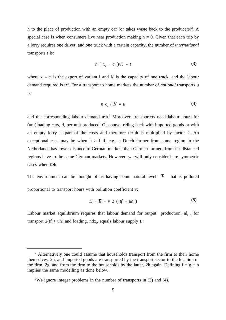
h to the place of production with an empty car (or takes waste back to the producers)2. A

special case is when consumers live near production making h = 0. Given that each trip by

a lorry requires one driver, and one truck with a certain capacity, the number ofinternational

transports t is:

where xi - ci is the export of variant i and K is the capacity of one truck, and the labour

(3)n ( xi ci )/K t

demand required is t•f. For a transport to home markets the number ofnational transports u

is:

and the corresponding labour demand u•h.3 Moreover, transporters need labour hours for

(4)n ci / K u

(un-)loading cars, d, per unit produced. Of course, riding back with imported goods or with

an empty lorry is part of the costs and therefore tf+uh is multiplied by factor 2. An

exceptional case may be when h > f if, e.g., a Dutch farmer from some region in the

Netherlands has lower distance to German markets than German farmers from far distanced

regions have to the same German markets. However, we will only consider here symmetric

cases when f≥h.

The environment can be thought of as having some natural level that is pollutedE

proportional to transport hours with pollution coefficient v:

Labour market equilibrium requires that labour demand for output production, nli , for

(5)E E v 2 ( tf uh )

transport 2(tf + uh) and loading, ndxi, equals labour supply L:

2 Alternatively one could assume that households transport from the firm to their homethemselves, 2h, and imported goods are transported by the transport sector to the location ofthe firm, 2g, and from the firm to the households by the latter, 2h again. Defining f = g + himplies the same modelling as done below.

3We ignore integer problems in the number of transports in (3) and (4).

5

(6)n li 2 t f 2 u h n d xi L 0

For the resulting hours of pollution the transport firm pays a tax or a price, s, for pollution

rights owned by the households of, in sum

to households. Given (5) households thus receive a payment of

s2 ( tf uh )

s 2 ( tf uh ) s ( E E )/v

3. The decisions of the households and the producers

The Lagrange function for the problem of households - with pi and representing pricesp̃j

of home and foreign goods respectively and w the wage rate - is:

The first-order conditions for the problem of the household are:

Maxci,c̃j, λ, E

Un

i

c θi

n n

n 1

c̃ θj V(E) λ{ wL

n

1

pi ci

n n

n 1

p̃j c̃j s (E E)/v}

(10) delivers the desired level of environmental quality, E. If the desired E equals the actual

(7)δU / δci θc θ 1i λpi 0 i 1,.....,n

(8)δ U / δ c̃j θ c̃ θ 1j λ p̃j 0 j n 1,...,n n

(9)δU / δλ wLn

1

pici

n n

n 1

p̃jc̃j s (E E)/v 0

(10)δ U / δ E V λ s/v ≤ 0 (δ U/ δ E) E 0

one, the corresponding s will be called equilibrium tax or equilibrium price for pollution

6

rights. The inequality results from the possibility that households may want to sell all

pollution rights E. Whether or not this will be the case will depend on the specification of the

utility function V. We do not consider the other corner solution E = because no pollutionE

implies no transport and therefore zero consumption which cannot be an equilibrium situation.

From (7) and (8), we find the equality of the marginal rate of substitution and relative prices:

and therefore:

c θ 1i / c̃ θ 1

j pi / p̃j

The computation of the price elasticity of demand for a large number of goods can be

(11)p̃jcθ 1i / c̃ θ 1

j pi

approximated by

Within the simple model assumed here, producer prices, the terms in square brackets

δ pi / δ ci (ci / pi) θ 1

in the profit function below, are equal to consumer prices, p, net of transportation costs4. If

external costs are 20% of transport costs or revenues, the Pigovian value of s is s = 0.2w

because transport costs consist only of wages in our simple model. The profit function of the

monopolist is:

where xi - ci = because of the assumption that countries are identical and that goods enter

πi [pi(ci) dw (w s)2h/K] ci [p̃j(c̃j) dw (w s)2f/K](xi ci)

{ wα wβ(ci xi ci)}

c̃j

the utility functions symmetrically.

Maximizing the profit function with respect to ci and yields:c̃j

4The relationship between the monopolist and the transporter is modelled in appendix A,which is available upon request.

7

δ π / δci pi ci [pi (ci) d w (w s) 2h /K] w β 0

δ π / δ c̃j p̃j c̃j [p̃j (c̃j) dw (w s)2f /K] w β 0

4. Solution of the model

Using the fact that the price elasticity isθ-1 and setting w = 1 theprevious equations can be

solved and yield:

From these expressions for prices we find proposition 1.

pi [β d (1 s) 2h / K]/θ ≡ η / θ

p̃j [β d (1 s) 2f / K]/θ ≡ ϕ / θ

PROPOSITION 1: Technical progress in variable labour inputs, dβ, in (un-) loading, dd <

0, in capacity, dK > 0, and in speed of driving, dh, df < 0, all considered at constant

pollution v per hour, reduces the prices of home and foreign goods and therefore increases

real wages.

As the terms in square brackets in the equations above differ only in the distances h

and f, we henceforth use and to abbreviate them. The result for pi differs from thatη ϕ

in Krugman (1983) because we have introduced transport costs for national trade. In our

model the price ratio contains three cost terms whereas under Krugman’s iceberg costs

assumption, it equals the share of not melting away during transport. The difference between

the two price equations mirrors the difference between h and f. Another essential result is

stated in proposition 2.

PROPOSITION 2: Payments for the environment drive prices up and real wages down. As

a consequence the monopolistic inefficiency, defined as the deviation of marginal cost (β),

plus transport costs from prices, increases.

As has been pointed out by Buchanan (1969), who derived a similar result in a partial

equilibrium model, this has to be taken into account when looking for an optimal subsidy as

we do below in section 8. However, as transport costs are crucial here we find the following

8

result;

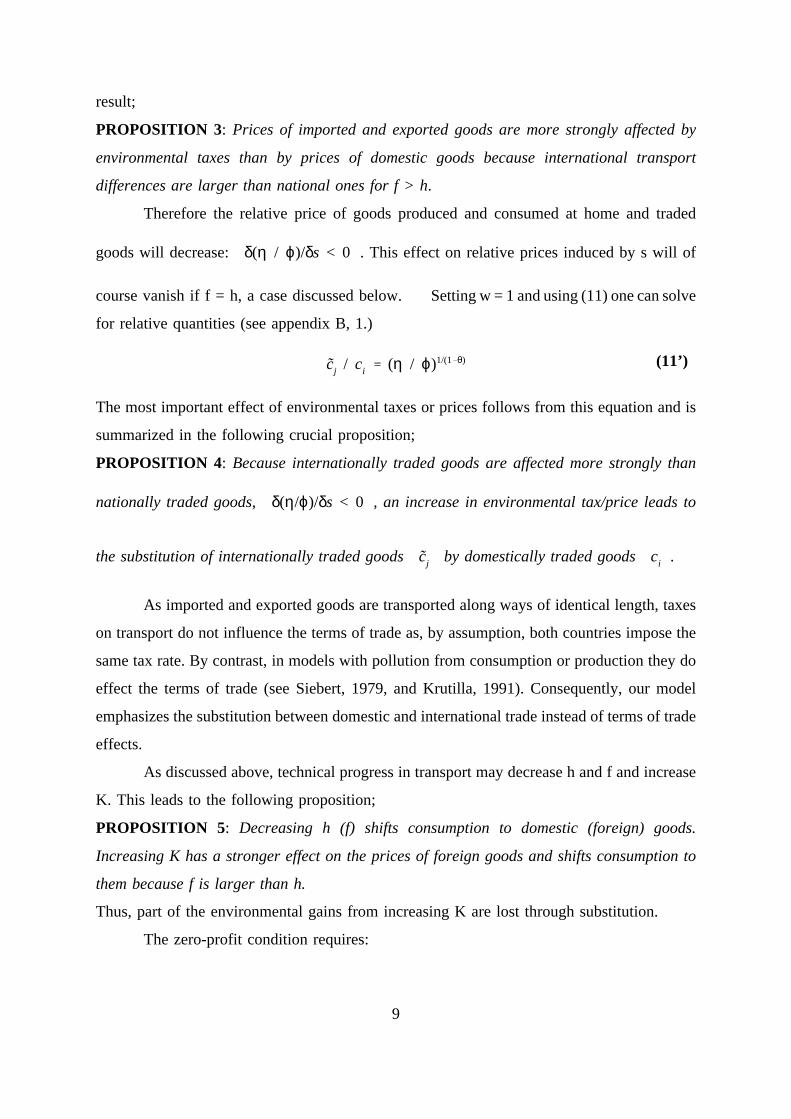
PROPOSITION 3: Prices of imported and exported goods are more strongly affected by

environmental taxes than by prices of domestic goods because international transport

differences are larger than national ones for f > h .

Therefore the relative price of goods produced and consumed at home and traded

goods will decrease: . This effect on relative prices induced by s will ofδ(η / ϕ)/δs < 0

course vanish if f = h, a case discussed below. Setting w = 1 and using (11) one can solve

for relative quantities (see appendix B, 1.)

The most important effect of environmental taxes or prices follows from this equation and is

(11’)c̃j / ci (η / ϕ)1/(1 θ)

summarized in the following crucial proposition;

PROPOSITION 4: Because internationally traded goods are affected more strongly than

nationally traded goods, , an increase in environmental tax/price leads toδ(η/ϕ)/δs < 0

the substitution of internationally traded goods by domestically traded goods .c̃j ci

As imported and exported goods are transported along ways of identical length, taxes

on transport do not influence the terms of trade as, by assumption, both countries impose the

same tax rate. By contrast, in models with pollution from consumption or production they do

effect the terms of trade (see Siebert, 1979, and Krutilla, 1991). Consequently, our model

emphasizes the substitution between domestic and international trade instead of terms of trade

effects.

As discussed above, technical progress in transport may decrease h and f and increase

K. This leads to the following proposition;

PROPOSITION 5: Decreasing h (f) shifts consumption to domestic (foreign) goods.

Increasing K has a stronger effect on the prices of foreign goods and shifts consumption to

them because f is larger than h.

Thus, part of the environmental gains from increasing K are lost through substitution.

The zero-profit condition requires:

9

The last two equations could be solved for ci and . Replacing pi, pj and cj in the zero

[pi dw (w s) 2h / K] ci [p̃j dw (w s) 2f / K] c̃j { w α w β (ci c̃j)} 0

c̃j

profit equation and using the abbreviations mentioned above yields (see appendix B, 2.):

c fi

[α θ/(1 θ)]/ϕη/ϕ (η/ϕ) 1/(θ 1)

The upper index f stands for "free trade". The first term represents domestic consumption of

c̃ fj

[ α θ1 θ

/ϕ ] (η/ϕ ) 1/(θ 1)

η/ϕ (η/ϕ) 1/(θ 1)

domestically produced goods. The second terms represents export quantities which is equal

to the amount of domestic consumption of foreign goods under the assumption of two

identical countries. For f = h, prices of traded and domestic goods are identical and the

increase ofϕ through an increase of s will reduce the consumption of both goods by the same

amount. As f > h induces a substitution of for ci, it is clear that whereasc̃j δc̃j / δs < 0

the substitution effect may prevent ci from falling if s increases. With these solutions for

prices and quantities we can now go back to equation (6) and solve for n, the number of

domestically produced varieties. Insertion of (2) and the definitions of t, u and xi into (6) after

collecting c-terms and insertion of the free trade solutions for the c-terms yields (see appendix

B, 3.):

As the effect of the c-terms on nf is negative, the effect of s on nf, is:

n f [ci (β 2h / K d) α c̃j (β 2f / K d)] 1 L

{[ α θ / (1 θ)]/ϕ} {( β 2h / K d) (η/ϕ) 1/(θ 1) (β 2f / K d))

η/ϕ (η/ϕ) 1/(θ 1)α

1

L

10

where the latter condition is fulfilled if f - h is sufficiently small, as discussed above. Whereas

δ n f / δ s (δ n / δ ci) (δ ci / δ s) (δn / δ c̃j) (δ c̃j / δs) > 0 if δ ci / δs < 0

in comparative advantage models the export structure may be reversed if exporters are heavily

taxed by one country only (see Pethig, 1976 and Siebert 1977, 1979 on the theory and

Grossman/Krueger 1991 on the empirics) this, of course, cannot be the case in a symmetric

model whereby the pollution of transport is taxed by both countries. Instead we get the

following proposition;

PROPOSITION 6: Both countries will produce a higher number of varieties, at least if

national and international transport differences are sufficiently small. Bringing the

environmental costs correctly into the cost calculations through taxes and transferring the tax

revenues to households increases variety and decreases quantity.

This is achieved through the revenues from transport and pollution due to taxation. For

f = h the reduction in pollution is5 :

The following proposition follows from this inequality;

δ {[ vn (ci h c̃j f) / K]} / δ s 4 f 2 L θ v (θ 1)

{ β k dk 2f [s (θ 1) 1]} 2< 0

PROPOSITION 7: The increase in the number of varieties, induced by a higher tax rate, is

smaller than the change in the quantities because new varieties require fixed labourci , c̃j

inputsα. Therefore the induced substitution of quantity for variety and of international for

domestic transport reduce pollution.

Using the definitions ofϕ and η one can now show6 that without environmental

policy, s = 0:

Without environmental policy, s = 0, transport costs have no influence on the number of

n f (1 θ) L / α

5This result can be obtained by differentiation of the left-hand side with respect to n, ci,c*

j, and differentiating them with respect to the environmental tax/prices according to the partsof the solution derived above.

6Without environmental policy we haveη = β + 2h/K +d, andϕ = β + 2f/K + d.

11

varieties. The corresponding solution for n* would be determined in the foreign countries’

symmetric model. With the solution for n one can go back to (5) and solve for - E, theE

environmental costs, using (3) and (4) and the solutions for consumption of domestic and

foreign goods. Before doing that we compute the solution of the model for autarky which we

will subsequently need to calculate the gains from trade.

5. The solution for autarky

As n* is given, free trade could only be identical to autarky if would go be zero in thec̃j

utility function. This in turn can only be the case ifϕ goes to infinity which would require

to have infinitely high prices . Thus, unlike comparative advantage models, autarkyp̃j

cannot be thought of as a special case of trade where the terms of trade equal autarky prices.

In autarky we have ci = xi , 0 = n* = t = and does not exist. The zero profitc̃j p̃j

condition solved for ci yields (see appendix B, 4.):

The upper index ’a’ stands for ’autarky’. From the definition ofη it is clear that the following

c ai α θ / [η (1 θ)]

proposition can be derived.

PROPOSITION 8: Environmental payments reduce the quantity consumed of each variety

whereas technical progress in transport, dh < 0, and in capacity dK > 0, increase it.

Modifying (6), solving for n and inserting the solution of ci yields (see appendix B,

5.)

If there were no environmental payments (s = 0) the solution for the number of varieties in

n a L (1 θ)

[β d (1 s) 2h / K][β d (1 s) 2h / K] θ s 2h / K

/α

autarky would be that of the Krugman model without transport costs. Differentiating na with

12

respect to the domestic transport distance, h, and the environmental payment, s, yields the

following proposition.

PROPOSITION 9: (a) For any environmental payment s > 0, an increase in national

transport costs, dh > 0, increases the number of varieties available under autarky. (b)

Environmental payments increase the autarkic number of firms because household income

increases proportionally to the environment being taxed or "rented out" to the transport firm.

This holds because the rebatement of tax revenues and the decreased quantity

consumed of each variety compensates households for the loss in environmental quality

associated with each unit of emission rights bought by the transport firm.

6. Gains from free trade reconsidered

To consider the conventional gains from trade net of the utility losses from pollution we

consider the difference between utility levels under free trade and under autarky using (1)

where we fill in the elements of the solution to the model:

Due to the symmetry assumption of the model we have nf = n*f . Using n*a = = 0 and

G ≡ U f U a n f (c fi )θ (n )f(c̃ f

j )θ V(E f) [n a(c ai )θ (n )a(c̃ a

j )θ V(E a)]

c̃ aj

(3)-(5) the gains from trade can be written as:

Considering the case of no environmental payments, s = 0, we have nf = na, henceforth

G U f U a

n f [(c fi )θ (c̃ f

j )θ] n a (c ai )θ V [E 2vn f (c̃ f

j f c fi h) / K] V[E 2vn a c a

i h / K]

abbreviated as n and for V(E) = E we find:

The first term contains the conventional gains from trade for the model with transport costs

G U f U a n [(c fi )θ (c̃ f

j )θ (c ai )θ] 2vn (c̃ f

j f c fi h c a

i h) / K

and no environmental policy and the second the expected losses from the increased pollution

due to increased transport costs. Insertion of the values for n and the c-terms yields after some

manipulation (see appendix B, 6.):

13

The first of the two terms in braces contains the conventional gains from trade which are

G L (1 θ) α 1

{( α θ/ϕ1 θ

)θ

[1 (η/ϕ)θ / (1 θ)] [1 ( ηϕ

)θ

1 θ ]θ

[η/ϕ (η/ϕ)1/(1 θ)]θ

2v { α θ / ϕ1 θ

(η/ϕ) 1 / (θ 1) f h ( ηϕ

)θ

1 θ

η/ϕ (η/ϕ) 1 / (θ 1)/K}

positive asθ < 1 and the second the expected losses from the increased pollution due to

increased transport costs which has the expected sign for f > h and θ < 1. As v does not

appear inη andϕ, it does not appear in the formula for the conventional gains from trade.

This yields the following proposition;

PROPOSITION 10: If the pollution per unit of transport v is sufficiently high the

conventional gains from trade may be outweighed by the environmental losses from increased

transport pollution.

This result had already been derived by Pethig (1976) and Siebert (1977) but in a comparative

advantage model of perfect competition with pollution from output production under the

additional assumption that the country in question specializes in the environment-intensive

good.

Whether or not this is the case is clearly an empirical question, which we cannot

address here. Grossman and Krueger (1991) cast some doubt on the empirical relevance of

the shift to pollution-intensive production induced by trade. However, in this paper the result

is restated here for an extension of the Krugman model based on pollution from transport,

which does not depend on such a shift. Moreover, unlike Pethig’s result that trade has no

impact on pollution once environmental capital is fixed by an environmental standard, here

trade inevitably increases pollution because international transport differences are longer than

the national ones and transport is complementary to production and consumption.

Of course the assumption made in many trade policy circles, such as GATT or now

WTO, that the welfare gains from free trade will "automatically" provide the means for

payments to reduce pollution, are clearly subject to the same empirical evaluation because it

14

ignores the pollution aspect of trade, i.e. the movement of goods through transport, itself.

7. Equilibrium prices for pollution rights

For s to be an equilibrium value the actual level of the environmental quality according to (5)

must be equal to the desired one according to (10) which requires formally:

or E = 0

(10’)V [ E v(tf uh) 2] λ s/v 0

In the latter case the household sells all emission rights because the return s is always higher

than marginal utility of the environment: s > vV’/λ.

The value of s in the first case is:

Insertion of values for n and the c terms delivers:

s v V [E v ( tf uh )2 ] / λ v V { E v2n [fc̃j hci ]/K } / λ

(10’’)

s v V { E v2

{[ αθ/(1 θ)]/ϕ} [(β 2h/K d) (η/ϕ) 1/(θ 1)(β 2f/K d)]

η/ϕ (η/ϕ) 1/(θ 1)α

1

L

[f[ α θ1 θ

/ϕ](η/ϕ) 1/(θ 1)

η/ϕ (η/ϕ) 1/(θ 1)h [αθ/(1 θ)]/ϕ

η/ϕ (η/ϕ) 1/(θ 1)]/K}

v V { E v2 L {[ αθ/(1 θ)]/ϕ}{ f (η/ϕ) 1/(θ 1) h]/K

{[ αθ/(1 θ)]/ϕ}[( β 2h/K d) (η/ϕ) 1/(θ 1)(β 2f/K d)]}

v V { E v2 L{ f (η/ϕ) 1/(θ 1) h}/ K

[(β 2h/K d) (η/ϕ) 1/(θ 1)(β 2f/K d)]}

The argument in V’ contains the equilibrium level of environmental resources. The part

subtracted from is the equilibrium level of the environmental damage. As s is alsoE

contained inη and ϕ a solution of s can only be found for specifications of V(E). We

15

consider three cases.

Firstly, the specification V(E) = E implies V’ = 1 and s≥ v/λ. The equilibrium price

for pollution rights is v/λ or at s > v/λ > 0 the households sell all rights such that E = 0

because s > vV’/λ.

Secondly, the specification V(E) = Eθ and V’ = θ E(θ-1) is used. Here we must get the

internal solution of (10’), because for E = 0 marginal utility from the environment would go

to infinity. Therefore the household will always keep some rights.

Thirdly, we assume V(E) = ln E implying V’ = E-1 . As a result, and under the additional

simplifying assumption f = h, we get anon-unique equilibrium value for the tax/subsidy:

In the first term SQRT B is an abbreviation for the square root of some lengthy expression

s± B

4 E f (θ 1)

βK4f(θ 1)

dK4f(θ 1)

v(θ 1 L θ)

E 2 (θ 1)

12(θ 1)

B. Only the second but last term is positive forL > 1 . If f, v and L aresufficiently large

then the sum of the last four terms is positive. Together with the negative SQRT B the

equilibrium tax is positive for high transport costs f, strong pollution v and a large market

expressed through high L if people value the environment sufficiently higher as its quality

decreases. A negative solution can be ruled out because again marginal utility would be at

infinity which induces households to keep some rights.

8. Optimal taxes and subsidies

The consideration of optimal taxes or subsidies is interesting for two reasons. For one,

because of the fact that equilibrium and optimal solutions to the environmental externality will

not be identical in this model because there is also a monopolistic inefficiency and because

the endogenous number of products exerts an externality on households. The literature

considering the deviation of optimal from equilibrium taxes/subsidies is of the partial

equilibrium type following Buchanan (1969). Two, after having shown in the previous section

that the existence of equilibrium taxes/subsidies may lead to a complete selling of

environmental rights, it is interesting to see which results follow from tax policy analysis.

Although there are three imperfections (the number of varieties is given to the households but

endogenous to the model, monopolistic prices deviate from marginal costs and there is no

16

market for pollution rights) we use only one instrument, pollution taxes. The motivation is

that under zero profits governments will hardly interfere with monopoly and the variety

externality will supposedly be ignored as well.

Again we consider the three specifications given above. The solutions for the number

of varieties, domestic and imported consumption goods, are inserted into the utility function,

which is maximized with respect to the environmental tax/subsidy, s. We report the results

only.

For V(E) = E and V’ = 1 wefind the optimal tax/subsidy as the implicit solution of:

Suppose s > 0, then f≥h andθ < 1 lead to a contradiction because all terms on the left side

[fhs (2 θ 2) β K (f h θ) dK (f h θ) fh (2 θ 2)]

[ 2hs β K dK 2h2fs β K dK 2f

]1/(θ 1) f 2 s(2θ 2) f (θ 1) (β K dK 2f) 0

of the equation are negative. Therefore we get the following proposition;

PROPOSITION 11: Under a linear utility function the tax s must be negative whereas it was

positive in the corresponding market equilibrium. The reason is that a positive tax would

decrease pollution and is likely to increase the number of varieties and therefore it also

increases the monopolistic inefficiency of prices deviating from marginal costsβ. This latter

inefficiency is dominating with the specification at hand.

This is a general equilibrium formulation of Buchanan’s (1969) problem. Even if

environmental quality would go to zero, marginal utility is not increasing because of the

assumption of a linear utility function. The value of the environment is thus constant whereas

the value of the foregone consumption goods under a positive tax is increasing if consumption

is reduced and the monopolistic inefficiency is increased (decreased) by a positive (negative)

tax.

The simplest next step is again to give the environment the same elasticity of utility

as consumption, namelyθ. This leads to the following proposition;

PROPOSITION 12: For V(E) = Eθ and V’ = θ Eθ-1, the case where no market equilibrium

existed in the previous section, we find an optimal tax/subsidy s = 0 for the simplification h

= f. For positive taxes the increase in the monopolistic inefficiency would more than outweigh

the sum of the environmental gains and the increase in utility through an increase in the

number of varieties.

17

However, if f > h, an increase in environmental taxes, ds > 0, is likely to shift

transport services and demand from international to national transport. Therefore an optimal

subsidy may be positive for f > h.

The result of a tax at level zero for f = h may beviewed as counterintuitive in view

of the urgency of some environmental problems. Therefore we increase the marginal utility

of low values of environmental quality even further, assuming V(E) = ln E and V’ = E-1 . As

a condition for positivity of the optimal tax for f = h we nowget:

To derive a condition for s > 0 wedivide this expression by s 0, which yields the

{ E f s2(4 θ2 8 θ 4) 2s(θ 1)[β E K d E K 2f (E L θ v)]} > 0

>(<)

condition:

As the denominator is positive we find the following proposition;

s >(<)

2 (θ 1)[ β E K d E Kf

2 (E L θ v)]

E 4 (θ2 2 θ 1)

PROPOSITION 13: For sufficiently high values of the pollution coefficient v and the size

of the market L, the right side is positive and therefore a tax (s) will have to be positive as

it was under similar conditions in the market equilibrium considered in the previous section.

A growing economy which is captured through growth in L here requires a positive tax after

some time and growing taxation once the tax is positive7.

Generally speaking, positive optimal taxes require a utility function that is steeper in

the environmental part than in that of the quantities. Otherwise optimal taxes may be negative

or zero, because the monopolistic inefficiency is dominating. Unlike Buchanan (1969), we

derived the exact assumptions that are underlying these results in a general equilibrium

framework.

7 Sinclair (1992) argues that this may be an incentive to increase resource extraction inthe short run where producer prices for carbon fuel are high. We assume here that resourceextraction policy will not counteract international agreements to increase taxes and reducepollution.

18

9. Conclusion

Since we have put the results in the form of propositions we do not summarize them again

here.

The policy results of our model depend strongly on peoples’ preferences for

environmental quality, which may be quite different among individuals, and on the severity

of pollution itself, which under imperfect information is highly subjective.

In our view the most interesting case in the model is the one where taxes on pollution

are positive because the underlying preferences seem to mirror the urgency of the

environmental problem more adequately. However, the main implication of our analysis, is

the relatively straightforward illustration that under ’realistic’ assumptions, the market solution

is not only necessarily non-optimal.

As illustrated in section 8, growing taxes on pollution seem to be a more reliable

general strategy towards optimal policy than any attempt to install "new pollution markets".

The latter will in the best case lead to a market equilibrium which will yield all the

"Pigovian" prices that have correctly been characterized by Buchanan as suboptimal.

This result is of course against economists’ intuition that markets do economize and allocate

better than governments. This intuition has, however, been formed under the impression of

traditional markets for which property rights had not to be established through the government

as is the case with pollution rights. Government action to distribute pollution rights and to

organize a market involves risks of both a market failure as well as government failure.

References

Barnett, A. H. (1980), The Pigouvian Tax Rule under Monopoly, in:American EconomicReview, 1037-1041.

Buchanan, James M. (1969), External Diseconomies, Corrective Taxation and MarketStructure, in:American Economic Review, 174-177.

Conrad, K. (1993), Taxes and Subsidies for Pollution-Intensive Industries as Trade Policy, in:Journal of Environmental Economics and Management25, 121-135.

Dogs, Ernst, Gunther Ellwanger and Holger Platz (1991), Externe Kosten des Verkehrs, in:Die Bundesbahn 1, p.39-45.

19

Grossman, Gene M. and Alan B. Krueger (1991), Environmental Impacts of a NorthAmerican Free Trade Agreement,NBER Working PaperNo. 3914, November.

Judd, K. (1985), On the Performance of Patents, in:Econometrica, Vol. 53, No. 3, May, 567-585.

Katz, Lawrence F. and Lawrence H. Summers (1989), Industry Rents: Evidence andImplications, in:Brookings Papers on Economic Activity: Microeconomics, 209-290.

Krugman, P.R. (1979), Increasing Returns, Monopolistic Competition, and International Trade,Journal of International Economics9, 4 (November), 469-479.

Krugman, P.R. (1981), Intraindustry Specialization and the Gains from Trade, in:Journal ofPolitical Economy89, 5, 959-974.

Krugman, P. R. (1983), The ’New Theories’ of International Trade and the MultinationalEnterprise, in: C.P. Kindleberger and D.B. Audretsch,The Multinational Corporation in the1980s, MIT Press, Cambridge, Massachusetts, London, England.

Krutilla, Kerry (1991), Environmental Regulation in an Open Economy, in:Journal ofEnvironmental Economics and Management20, 127-142.

Lee, Dwight R. (1975), Efficiency of Pollution Taxation and Market Structure, in:Journalof Environmental Economics and Management2, 69-75.

Maks, J.A.H. (1994),Competition Policy and Imperfect Information, The Netherlands 1987-1992, METEOR Research Memorandum RM/0/94-034, 13p.

Markusen, James R., Edward R. Morey and Nancy Olewiler (1993),Environmental Policy when market structure and plant locations are endogenous, in:Journalof Environmental Economics and Management24, 69-86.

McGuire, M.C. (1982), Regulation, Factor Rewards, and International Trade, in:Journal ofPublic Economics17, 335-354.

Merrifield, John D. (1988), The Impact of Selected Abatement Strategies on TransnationalPollution, the Terms of Trade, and Factor Rewards: A General Equilibrium Approach, in:Journal of Environmental Economics and Management15, 259-284.

Morrison, C.J. (1989),Unravelling the productivity growth slowdown in the U.S., Canada,and Japan, NBER Working Paper 2993.

Morrison, C.J. (1990),Market Power, Economic Profitability and Productivity GrowthMeasurement: An Integrated Structural Approached. NBER Working Paper 3355, May.

Morrison, C.J. (1992), Unravelling the Productivity Growth Slowdown in the United States,Canada and Japan: The Effects of Subequilibrium, Scale Economies and Markups, in:The

20

Review of Economics and Statistics, Vol.LXXIV, August, Number 3, 381-93.

Pethig, Rüdiger (1976), Pollution, Welfare, and Environmental Policy in the Theory ofComparative Advantage, in:Journal of Environmental Economics and Management2,160-169.

Siebert, Horst (1977), Environmental Quality and the Gains from Trade, in:Kyklos, 30,657-673.

Siebert, Horst (1979), Environmental Policy in the Two-Country-Case, in:Zeitschrift fürNationalökonomie, (Journal of Economics), Vol. 39, 259-274.

Sinclair, P. (1992), High does nothing and rising is worse: carbon taxes should keep decliningto cut harmful emissions, in:The Manchester School, Vol. LX No. 1, March, 41-52.

Autorenhinweis:

Luc Soete, born 1950, studied economics at the Universities of Gent, Antwerp and Sussex.Professor International Economics at the Maastricht University and Director of the MaastrichtEconomic Research Institute on Innovation and Technology (MERIT). Major areas of interestInternational Economics and the Economics of Technical Change. Address: MERIT, P.O.Box616, NL-6200 MD Maastricht. e-mail: L.Soete@algec.unimaas.NL.

Thomas Ziesemer, born 1953, studied economics at the Universities of Kiel and Regensburg.Assistant professor international economics and associate professor microeconomics,Maastricht University. Fields of Interest: Growth theory, development, international,environmental and microeconomics, economics of technical change. Address: MERIT,P.O.Box 616, NL-6200 MD Maastricht. e-mail: T.Ziesemer@algec.unimaas.NL.

21