This is re-typesetting of the book first published as PUBLICATIONS OF THE MATHEMATICAL SOCIETY OF JAPAN 13 TWO APPLICATIONS OF LOGIC TO MATHEMATICS by Gaisi Takeuti Kanˆo Memorial Lectures 3 Iwanami Shoten, Publishers and Princeton University Press 1978 The present work was typeset by A M S-L A T E X, the T E X macro systems of the American Mathematical Society. T E X is the trademark of the American Mathematical Society. c ⃝2012 by the Mathematical Society of Japan. All rights reserved. The Mathematical Society of Japan retains the copyright of the present work. No part of this work may be reproduced, stored in a retrieval system, or transmitted, in any form or by any means, electronic, mechanical, photocopying, recording or otherwise, without the prior permission of the copy- right owner.
Transcript
This is re-typesetting of the book first published as
PUBLICATIONS OF THE MATHEMATICAL SOCIETY OF JAPAN13
TWO APPLICATIONS OF LOGICTO MATHEMATICS
by
Gaisi Takeuti
Kano Memorial Lectures 3
Iwanami Shoten, Publishersand
Princeton University Press
1978
The present work was typeset by AMS-LATEX, the TEX macro systems of theAmerican Mathematical Society.TEX is the trademark of the American Mathematical Society.
c⃝2012 by the Mathematical Society of Japan.
All rights reserved. The Mathematical Society of Japan retains the copyright ofthe present work. No part of this work may be reproduced, stored in a retrievalsystem, or transmitted, in any form or by any means, electronic, mechanical,photocopying, recording or otherwise, without the prior permission of the copy-right owner.
i
TWO APPLICATIONS OF LOGIC
TO MATHEMATICS
by Gaisi Takeuti
ii
Preface
This book consists of two independent parts, each of which has its own list ofreferences.
Part I is Boolean valued analysis. Most of the content of this part wasdiscussed in my courses in the spring semester of 1974 at the University ofIllinois and the summer semester of 1975 at the Universitat Heidelberg.
I appreciate the interest shown by my colleagues and I have profited fromdiscussions with them and from information and advice that they have pro-vided. In particular I want to recognize the assistance of Joseph Doob, PeterLoeb, Heinrich Lotz, Earl Berkson and especially David Berg for his instructivediscussion of Hilbert spaces.
Part II is titled “A conservative extension of Peano Arithmetic”. The contentis a revision of my lecture notes for a course offered in the fall semester of 1972at the University of Illinois. The revision was used in a course that I offered inthe summer semester of 1975 at the Universitat Heidelberg. I started this workin the course of correspondence with Georg Kreisel. I have profited from hiscorrespondence. The original lecture notes were prepared with the assistance ofMariko Yasugi, and editorial assistance was provided by my colleague WilsonZaring. Mr. Mamoru Kurata and Mr. Susumu Hayasi have read the proofs ofPart I and Part II respectively.
This book was written at the suggestion of my teacher Professor S. Iyanaga.I also received encouragement from Professor Godel and I express my deepappreciation to him and to all who contributed.
Mathematical logic is reflection on mathematics. More specifically it is re-flection on such questions as, What is logical validity? What is effective cal-culability? What is a set? What are the basic principles of the universe ofsets. Apart from reflecting on these questions themselves, and proving relevantmetatheorems, one also wants to know the chances of an effective use of variouslogical metatheorems in specific branches of mathematics. For example, onemight say that Abraham Robinson’s non-standard analysis answers the ques-tion of how the completeness theorem can be put to good use in analysis, orthat Ax-Kochen theory answers the same question for the theory of ultra prod-ucts. This book offers two additional examples of such applications of logicalmetatheorems in specific branches of mathematics.
Part I is devoted to Boolean valued analysis, that is, it is devoted to anapplication of Scott-Solovay’s Boolean valued models of set theory to analysis.Our aim is to establish basic relation between elementary notion in Booleanvalued models and analysis.
In Chapter 1, we consider complete Boolean algebras of projections in Hilbertspace. Although the algebra of all projections (with their familiar operations)in a Hilbert space does not form a Boolean algebra, many complete Booleanalgebras are embedded there.
Let B be a complete Boolean algebra, let A be a self-adjoint operator with
spectral decomposition A =
∫λdEλ. The operator A is said to be in (B) if
Eλ ∈ B for every λ. If Aαα is a set of pairwise commutable self-adjointoperators, then there exists a complete Boolean algebra B of projections, suchthat Aα is in (B) for every α. The Boolean valued model of such a completeBoolean algebra B of projections has interesting interpretations in analysis. Forexample, the real numbers in such a model are exactly the self-adjoint operatorsin (B) and real number addition, multiplication and order correspond to theaddition, multiplication, and order of self-adjoint operators.
The convergence of reals in the model also has a close relation with theconvergence of self adjoint operators in the strong topology.
In chapter 2, we consider Boolean valued analysis using a measure algebrawhich is originally considered by Scott. Reals in this model correspond tomeasurable functions. We discuss the interpretations of Baire functions, Borelsets, differentiation, integration and the Baire category theorem in the model.
In Part II, we discuss a conservative extension of Peano arithmetic, i.e., anapplication of Gentzen’s cut elimination theorem. Here we take a very weaksystem of arithmetic with higher type and develop classical analysis in it. Thenature of the work is essentially expository. There are many similar worksby H. Weyl, G. Kreisel, P. Lorenzen, K. Schutte and many others. We placeemphasis on the following points.
1. We take a simple system whose proof-theoretic nature is very clear. Thecut elimination theorem implies that the system is a conservative exten-
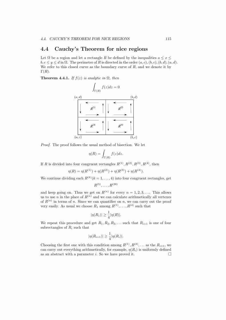
2 CONTENTS
sion of Peano arithmetic, i.e., every arithmetical statement proved in thesystem is a theorem of Peano’s arithmetic.
2. We are interested in classical logic and classical analysis. In particularwe are interested in classical analytic number theory. For this reason, wedevote special attention to the development of the theory of functions ofa complex variable.
From this, one can conclude that an arithmetical statement proved by themethod of classical analytic number theory is a theorem of Peano’s arithmetic.
Since we started this work in the course of correspondence with Kreisel,let us discuss his work on the subject. In his earlier work (part II [3], [4],[5], pp. 168–172, [12], [16]), Kreisel simply transcribed proofs in analysis intothe language of arithmetic with free function variables, by approximating theindividual functions in analysis, especially analytic number theory, by primitiverecursive functions on Q. In the late fifties (part II [9], [10], [11], [13], see also[6] pp. 327–328, 361–362, [7], very readable [8], [15], [17], [18], [19]) he switchedto an abstract language, i.e. a language with symbols for higher types but withweak existential axioms. However his main interest was not in conservativeextension over Peano’s arithmetic, but over the first few levels of the ramifiedhierarchy. In his lecture (unpublished and unavailable to us), he went back tothe old stuff on analytic number theory to show that the latter was conservativeover primitive recursive arithmetic.
Part I
Boolean Valued Analysis
3
5
In 1963, Paul J. Cohen introduced the notion of forcing and proved manyimportant independency results in set theory. In 1966, D. Scott and R. Solovayreformulated the theory of forcing in terms of Boolean valued models. (A similaridea was developed by Vopenka [12], [13].) We propose to apply the theory ofBoolean valued models to analysis. We will introduce the idea of a Booleanvalued model but without much explanation. However, the theory is easy tounderstand if one does several exercises after the basic properties of the modelare stated. We will assume the basic properties of self-adjoint operators andtheir spectral decompositions.
D. Scott not only started Boolean valued models of set theory, with Solovay,but also introduced Boolean valued analysis. His choice of complete Booleanalgebras was measure algebras. We will revisit Scott’s Boolean valued analysisin Chapter 2.
The idea of Boolean valued models goes back to Church [4] and Rasiowa andSikorski [8]. However it is fair to say that the success of Scott and Solovay’swork has encouraged many similar developments and applications.
Chapter 1
Boolean Valued AnalysisUsing Projection Algebras
1.1 Hilbert space
A bounded operator P , of a Hilbert space, is called a projection if P is self-adjoint and P 2 = P . We will use the symbol I to denote the identity operatori.e. Ix = x and 0 to denote an operator defined by 0 · x = 0.
A set B of projections is called a Boolean algebra of projections, if it satisfiesthe following conditions.
1. Both I and 0 are members of B and members of B are pairwise com-mutable.
2. If P1 and P2 are members of B, so are P1 ∨ P2, P1 ∧ P2, and ¬P1, whereP1 ∨ P2 = P1 + P2 − P1 · P2, PI ∧ P2 = P1 · P2, and ¬P1 = I − P1.
A Boolean algebra B of projections is said to be complete if B is not onlycomplete as a Boolean algebra but also satisfies the following condition. IfP = sup
αPα, then the range of P , denoted by R(P ), is the closure of the linear
space spanned by∪α
R(Pα).
From now on, let B be a complete Boolean algebra of projections. Let A
be a self-adjoint operator and let A =
∫λdEλ be its spectral decomposition.
Then A is said to be in (B) if for every real λ, Eλ is a member of B.
Let A and B be self-adjoint and let A =
∫λdEλ and B =
∫λdE′
λ be their
spectral decompositions. Then A and B are said to be commutable if for everypair λ, λ′ of reals
Eλ · E′λ′ = E′
λ′ · Eλ.
7
8CHAPTER 1. BOOLEANVALUEDANALYSIS USING PROJECTION ALGEBRAS
If A and B are bounded, then the commutativity of A and B is equivalent toA ·B = B ·A.
The following single fact is very useful in our work and will be used withoutmention.
Lemma 1.1.1. If Aα be a set of self-adjoint, pairwise commutable operators,then there exists a complete Boolean algebra of projections such that for everyα, Aα is in (B).
Let A and B be commutable self-adjoint operators. It is usual to defineA+B as the operator satisfying the conditions
D(A+B) = D(A) ∩ D(B) and
∀x ∈ D(A+B) (A+B)x = Ax+Bx,
where D(A) denotes the domain of A. The operator A+B, defined in this way,has a unique closed extension. For our purposes we define A + B to be thisunique closed extension. The operator A + B is also self-adjoint. In the sameway, A · B is defined to be the unique closed extension of the operator whichmaps x, with x ∈ D(B) and Bx ∈ D(A), to ABx. The operator A · B is alsoself-adjoint and A · B = B · A. Because of this definition, there is a possibilitythat A + B and/or A · B is defined on the whole Hilbert space, and thereforebounded, even if A and B are unbounded. In general, if the result of an operator0(A,B) is not closed but has a unique closed extension, we define 0(A,B) to bethe unique closed extension of the result.
An operator N is said to be normal, if N = A + iB where A and B areself-adjoint and commutable. Also N∗ = A− iB and NN∗ = N∗N = A2 +B2.Furthermore, N is said to be in (B), if A and B are in (B). We define |N | to be√A2 +B2. The operator |N | is self-adjoint.Let A and B be self-adjoint and commutable. Then A ≤ B if and only if for
every x ∈ D(A) ∩ D(B), (Ax, x) ≤ (Bx, x).
1.2 The model V (B)
In this section, we summarize the necessary back ground about the Booleanvalued model V (B) of set theory. For detail, see §13. and §16. in [10], though+, ·,−,Π,Σ are used there as Boolean operations in the place of ∨,∧,¬, inf, sup,and O and I are used in the place of 0 and I.
First we shall give a rough idea of V (B). Let D be a domain. A set ofmembers in D is decided by assigning true or false to x ∈ A for every memberx in D. A B-valued set of members in D is decided by assigning any elementP in B to x ∈ A for every member x in D. We write Jx ∈ AK = P if theassigned value of x ∈ A is P . The symbol ‘Jx ∈ AK = P ’ is read as ‘x ∈ Aholds with probability P ’. However, ‘Jx ∈ AK = I’ is read as ‘x ∈ A holds’ and‘Jx ∈ AK = 0’ is read as ‘x ∈ A does not hold’.
The universe V of all sets is obtained by starting with the empty set and bycreating sets of sets, sets of sets of sets etc. The Boolean valued universe V (B)
1.2. THE MODEL V (B) 9
is obtained by starting with the empty set and by creating Boolean valued setsof Boolean valued sets, Boolean valued sets of Boolean valued sets of Booleanvalued sets etc. By interpreting true by I and false by 0, there exists a naturalembedding, denoted by
√, of V into V (B) i.e.
√: V → V (B).
Let a ∈ V . The corresponding element in V (B) is denoted by√
a.Formally, we shall carry this out as follows. Let B be a complete Boolean al-
gebra (of projections). For an ordinal α, we define V(B)a by transfinite induction
as follows:
V(B)0 = ϕ
V (B)α = u|u : D(u) → B and D(u) ⊆
∪ξ<α
V(B)ξ
and V (B) =∪
α∈On
V (B)α ,
where On is the class of all ordinal numbers.It is easy to see that
1) if α is a limit, then V(B)α =
∪ξ<α
V(B)ξ ,
2) V(B)α+1 = u|u : D(u) → B and D(u) ⊆ V
(B)α , and
3) if α ≤ β, then V(B)α ⊆ V
(B)β .
For u, v ∈ V (B), Ju ∈ vK and Ju = vK are defined as functions fromV (B) × V (B) to B satisfying the following properties.
1. Ju ∈ vK = supy∈D(v)
(v(y) ∧ Ju = yK)2. Ju = vK = inf
x∈D(u)(u(x) ⇒ Jx ∈ vK) ∧ inf
y∈D(v)(v(y) ⇒ Jy ∈ uK)
where P1 ⇒ P2 is ¬P1 ∨ P2 i.e.
(I − P1) + P2 − (I − P1) · P2 = I − P1 + P1 · P2.
In the following, we also use ∧,∨,¬,⇒ as logical connections. Let φ be aformula in set theory, that is, let φ be obtained by applying logical symbols toatomic formulas of the form u ∈ v or u = v. If φ does not contain any freevariable and all the constants in φ are members in V (B), we define JφK by thefollowing rules.
1. J¬φK = ¬JφK = I− JφK
10CHAPTER 1. BOOLEANVALUEDANALYSIS USING PROJECTION ALGEBRAS
Jφ(u)KFrom this definition we have the following basic properties.
1. Ju = uK = I
2. Ju = vK = Jv = uK3. Ju1 = u2K · Ju2 = u3K ≤ Ju1 = u3K4. Ju = vK · Jφ(u)K ≤ Jφ(v)K5. Ju = vK = J∀x(x ∈ u iff x ∈ v)K.Since all the statements in analysis can be expressed in the language of set
theory, we can assign a value in B to any statement in analysis by J K.Let M = R(P ). Roughly the meaning of JφK = P is that φ holds if we
restrict our Boolean algebra B to a subspace M. In another words, the meaningof JφK = P is that φ does not hold if we restrict our Boolean algebra B to asubspace M⊥.
The theorem, which is the base of our work, is the following.
Theorem 1.2.1. The Boolean valued universe V (B) is a model of ZF set theorywith the axiom of choice. This set theory we denote by ZFC. In other words,if φ is a theorem of ZFC, then JφK = I i.e. φ holds in V (B).
Since every theorem in contemporary mathematics is a theorem in ZFC, wecan express this in the following way. If φ is a theorem, then φ holds in V (B).Moreover, from the proof of the Theorem 1.2.1, we have the following corollary.
Corollary 1.2.2. If φ is a theorem, then ‘φ holds in V (B)’ is also a theorem.
Since conditional is often used in mathematics, the following equivalence isuseful in practice
Jφ1 ⇒ φ2K = (Jφ1K ⇒ Jφ2K) and
(P1 ⇒ P2) = I iff P1 ≤ P2.
The following lemma which is Theorem 13.13. in [10] is also useful.
Lemma 1.2.3. For u ∈ V (B),
1. J∃x ∈ uφ(x)K = supx∈D(u)
u(x) · Jφ(x)K
1.2. THE MODEL V (B) 11
2. J∀x ∈ uφ(x)K = infx∈D(u)
(u(x) ⇒ Jφ(x)K).Now we define the embedding
√: V → V (B) precisely, by transfinite induc-
tion as follows.For y ∈ V ,
√
y= ⟨√
x, I⟩|x ∈ y
i.e.
√
y is a constant function such that D(
√
y) = √
x |x ∈ y and its value isconstantly I.
Obviously the following proposition holds.
Proposition 1.2.4 (Theorem 13.17. in [10]). For x, y ∈ V ,
1. x ∈ y iff J√x∈√
yK = I and
x ∈ y iff J√x∈√
yK = 0,
2. x = y iff J√x=√
yK = I and
x = y iff J√x=√
yK = 0.
In order to develop analysis in set theory, first the natural numbers areconstructed from ϕ, which is also denoted by 0, the integers are constructedas pairs of natural numbers, the rational numbers are constructed as pairs ofintegers, and finally, the real numbers are constructed by Dedekind’s cuts ofrational numbers. Since V (B) satisfies ZFC, we adopt the same definition ofthe natural numbers, integers, rational numbers and real numbers so that allthe theorems in analysis also hold in V (B). Let us denote the set of all naturalnumbers by ω, the set of all rational numbers by Q, the set of all real numbersby R and the set of all complex numbers by C. The first natural question is whatare ω,Q,R, and C in V (B). First two are answered as follows. (cf. pp. 129–130in [10]).
1. Let n be a natural number. Then n in V (B) is√
n. More precisely there existsa formula φ(x) which define n in the sense that ∃!xφ(x)∧φ(n) is provable.
Then ∃!xφ(x)∧φ(√
n) holds in V (B). In particular 0, in V (B), is
√
0, that is,√
ϕ is the empty set in V (B). In V (B), ω is√
ω.
Moreover√
n +√
m and√
n ·√
m, in V (B), are (n +m)√
and (n ·m)√
respectively.
Similarly√
n≤√
m iff n ≤ m.
2. Let r be a rational number. Then r, in V (B), is√
r . Moreover√
r1 +√
r2=
(r1 + r2)√
and√
r1 ·√
r2= (r1 · r2)√, hold in V (B). And,
√
r1≤√
r2 iff r1 ≤ r2.
12CHAPTER 1. BOOLEANVALUEDANALYSIS USING PROJECTION ALGEBRAS
Finally Q, in V (B), is
√
Q. We often write n, r, ω and Q in the place of√
n,√
r ,√
ω, and
√
Q. Note, in passing, that R, in V (B), may not be R. In many
cases, we can prove that J√R= RK = 0.
A subset Pα of B is called a partition of unity if the following conditionsare satisfied.
1. If α = β, then Pα · Pβ = 0.
2. I =∑α
Pα = supαPα,
where∑α
Pα is defined in the strong topology. Let Pα be a partition of unity
and let uα be a subset of V (B). Then there exists an element u of V (B) suchthat
∀α Ju = uαK ≥ Pα.
Moreover if there exists another u′ such that ∀α(Ju′ = uαK ≥ Pα), then Ju =
u′K = I, i.e. u = u′ holds in V (B). We denote this u by∑α
uαPα which is
determined uniquely in the sense of equality in V (B). (cf. Theorem 6.9. andCorollary 16.3. in [10]).
We call u ∈ V (B) a natural number in V (B), if Ju ∈ ωK = I. Now we would
like to see what the natural numbers in V (B) are. Let Ju ∈ ωK = Ju ∈√
ωK = I.Then
Ju ∈√
ωK = sup
x∈D(
√ω)
ω(x) · Ju = xK= sup
n∈ωJu =
√
nK.Let Pn = Ju =
√
nK. It is easy to see that Pn is a partition of unity and
u =∑n
√
n Pn =∑n
n · Pn.
There might be many 0’s among the Pn’s. Usually we take off the 0’s and write
u =∑i
ni · Pi,
where i ranges over a finite or infinite subset of ω.
Let Pi be a partition of unity, let ni be a subset of ω and let u =∑i
niPi.
Then it is easily seen that Ju ∈ ωK = I. Therefore all natural numbers in V (B)
are expressed in the form∑i
niPi. This form is very convenient for the following
reason. Let Pi and P ′j be two partitions of unity. Then Pi · P ′
jij is also
14CHAPTER 1. BOOLEANVALUEDANALYSIS USING PROJECTION ALGEBRAS
a partition of unity. Let u =∑i
niPi and v =∑j
mjP′j . Then the following
properties are easily checked.
u+ v =∑i,j
(ni +mj)Pi · P ′j
u · v =∑i,j
(ni ·mj)Pi · P ′j
Ju < vK = supPi · P ′j |ni < mj.
Let u ∈ V (B). Then u is called a rational number in V (B), if Ju ∈ QK = I. SinceQ is obtained from ω by a simple construction, what we proved about ω is alsotrue for Q, that is, the following properties hold.
1. All rational numbers in V (B) are those of the form∑i
riPi where Pi is
a partition of unity and ri is a subset of Q.
2. Let u =∑
riPi and v =∑j
r′jP′j be two rational numbers in V (B). Then
u+ v =∑i,j
(ri + r′j)Pi · P ′j
u · v =∑i,j
(ri · r′j) · Pi · P ′j
Ju ≤ vK = supPi · P ′j |ri ≤ r′jJu < vK = supPi · P ′j |ri < r′j.
Theorem 1.2.8 (The Maximum Principle, Theorem 16.2. in [10]). Let φ be aformula. Then there exists a u ∈ V (B) such that
Jφ(u)K = J∃xφ(x)K.Since J∃xφ(x)K = sup
v∈V (B)
Jφ(v)K, the meaning of the theorem is that there
exists a u which maximizes the value of Jφ(u)K.Let φ(x) be a formula with only x as a free variable. Let v0 ∈ V (B) satisfyJφ(v0)K = I. Now consider a statement of the form ∀x(φ(x) ⇒ ψ(x)). SinceJ∀x(φ(x) ⇒ ψ(x))K = inf
u∈V (B)Jφ(u) ⇒ ψ(u)K, we have to calculate Jφ(u) ⇒ ψ(u)K
for every u ∈ V (B) in order to calculate J∀x(φ(x) ⇒ ψ(x))K. Let u ∈ V (B) andJφ(u)K = P . Define u′ = u · P + v0 · (I − P ). It is easily seen that Jφ(u′)K = Iand Jψ(u′)K ≤ (Jφ(u)K ⇒ Jψ(u)K).Therefore we have
J∀x(φ(x) ⇒ ψ(x))K = infJφ(u)K=IJψ(u)K.
1.3. REAL NUMBERS IN V (B) 15
In the same way, we have
J∃x(φ(x) ∧ ψ(x))K = supJφ(u)K=I
Jψ(u)K.This justifies the following definition. We define the interpretation of x|φ(x)with respect to V (B) to be u ∈ V (B)|Jφ(u)K = I, assuming that it is not empty.
The above discussion shows that the interpretation of important notions inanalysis is at the center of our work.
Remark. Let u ∈ V (B). Then the class v ∈ V (B)|Ju = vK = I is always aproper class. This sometimes causes a technical inconvenience. In the following,we always think that we have picked up a representative from an equivalent classv ∈ V (B)|Ju = vK = I. Technically we use a set v ∈ V (B)|v is of the lowestrank with Ju = vK = I to represent a proper class v ∈ V (B)|Ju = vK = I. Inthis way, we can avoid the use of a uniform choice function.
1.3 Real numbers in V (B)
We define real numbers by Dedekind cuts. More precisely, by a real numberwe mean a set of rational numbers which is the upper segment of a Dedekindcut. If a is a real number and a corresponds to a rational number r, then weinclude r in a, that is r is the smallest member of a. Thus ‘a is a real number’is expressed by the following formula.
a ⊆ Q ∧ ∃s ∈ Q(s ∈ a) ∧ ∃s ∈ Q(s /∈ a) ∧ ∀s ∈ Q(s ∈ a ⇔ ∀t ∈ Q(s < t ⇒t ∈ a))
We define R(B) to be the interpretation of R in V (B), i.e.
R(B) = u ∈ V (B)|Ju is a realK = I.
Let u ∈ R(B) and r ∈ Q. We define Pr to be Jr ∈ uK. Then the following iseasily checked.
1. infr∈Q
Pr = 0
2. supr∈Q
Pr = I
3. Pr = infr<s
Ps.
Let λ range over real numbers. Let Eλ = infλ<r
Pr. Then
1. infλEλ = 0
2. supλEλ = I
3. Eλ = infλ<µ
Eµ.
16CHAPTER 1. BOOLEANVALUEDANALYSIS USING PROJECTION ALGEBRAS
This implies that Eλ is a resolution of the identity in (B). On the other hand,let Eλ be a resolution of the identity in (B). Let Pr = Er for each rationalnumber r, and define u to be a function satisfying
D(u) = r|r ∈ Q and u(r) = Pr.
Then u ∈ R(B) is easily checked and the correspondence between R(B) and theset of all resolutions of the identity in (B) is 1-1 onto. Since there is a 1-1 ontocorrespondence between the set of all resolutions of the identity in (B) and theset of all self-adjoint operators in (B), this establishes a 1-1 onto correspondencebetween the set of all self-adjoint operators in (B) and R(B). From now on, weexpress this relation by simply saying that the interpretation of a real number inV (B) is a self-adjoint operator in (B). We are going to investigate the meaningof addition, multiplication and ≤ for real numbers in V (B) as operations and arelation for self-adjoint operators in (B).
For a ∈ R, a ∈ R(B). Furthermore a represents a resolution of the identityEλ such that Eλ = 0 if λ < a and Eλ = I if a ≤ λ. Therefore a represents anoperator a · I i.e. a itself.
Though ω = ω and Q = Q hold, R = R does not hold in many Booleanvalued universes V (B). For example, take L2(−∞,∞), a self-adjoint operatorx·, and any complete Boolean algebra B such that x· is in (B). Let u ∈ R(B)
correspond to x·. In order to prove that JR = RK = 0, it suffices to show thatJu ∈ RK = 0 since Ju ∈ RK = I. Therefore it suffices to show that Ja = uK = 0for every a ∈ R.
Ja = uK = infr∈Q
Jr ∈ a⇔ r ∈ uK and
Jr ∈ a⇔ r ∈ uK = Jr ∈ uK if a ≤ rI − Jr ∈ uK if r < a.
Let x· =∫λdEλ. Then Jr ∈ uK = Er. Therefore Ja = uK = Ea − Ea−0 = 0.
The meaning of this fact is that there are many reals in V (B) that can not be
expressed in the form∑α
aαPα, where Pα is a partition of unity and aα is
a subset of R. It also means that there are lots of self-adjoint operators in (B)which are not of the form
∑α
aαPα.
Let u and v be in R(B). Let A =
∫λdEλ and B =
∫λdE′
λ be corresponding
self-adjoint operators in (B) respectively. We proceed to see what the basicoperations for u and v correspond for A and B.
Proposition 1.3.1. The sum u+ v corresponds to A+B.
Proof. Let a and b be real numbers. The addition for the upper segment ofDedekind cuts is defined in the following way.
r ∈ (a+ b) iff ∀s ∈ Q(r < s⇒ ∃t1, t2 ∈ Q(s = t1 + t2 ∧ t1 ∈ a ∧ t2 ∈ b))
1.3. REAL NUMBERS IN V (B) 17
Interpreting this in V (B), u+ v corresponds to an operator
∫λdE′′
λ such that
E′′λ = inf
λ<λ′supµEµ · E′
λ′−µ.
It is easily checked that A+B =
∫λdE′′
λ .
Proposition 1.3.2. The inequality u ≤ v holds in V (B) iff A ≤ B.
Proof. By definition, u ≤ v, for two reals defined by Dedekind cuts, if v ⊆ u.So
Ju ≤ vK = I iff J∀r ∈ Q(r ∈ v ⇒ r ∈ u)K = I
iff ∀r ∈ Q((I − E′r) + Er − Er · (I − E′
r) = I)
iff ∀r ∈ Q(E′r = Er · E′
r)
iff ∀r ∈ Q(E′r ≤ Er)
iff A ≤ B.
Proposition 1.3.3. Let A =
∫λdEλ be in (B). Let P ∈ B and AP =
∫λdE′
λ.
Then
E′λ =
Eλ · P + (I − P ) if λ ≥ 0Eλ · P otherwise.
Proof. Case 1) Px = x ∫λdE′
λx =
∫λdEλx = Ax
Case 2) Px = 0 ∫λdE′
λx =
∫ ∞
0
λd(Ix) = 0.
Proposition 1.3.4. Let A =
∫λdEλ and B =
∫λdE′
λ be in (B) and let
P ∈ B. Then
AP ≤ BP iff E′λP ≤ EλP for every λ.
Proof. AP ≤ BP iff Eλ · P + (I − P ) ≥ E′λ · P + (I − P ) for each λ ≥ 0
and
EλP ≥ E′λP iff EλP ≥ E′
λP for each λ < 0.
18CHAPTER 1. BOOLEANVALUEDANALYSIS USING PROJECTION ALGEBRAS
Proposition 1.3.5. Ju ≤ vK ≥ P iff AP ≤ BP.
Proof.
Ju ≤ vK ≥ P iff J∀r ∈ Q(r ∈ v ⇒ r ∈ u)K ≥ P
iff ∀r ∈ Q((I − E′r) + Er − (I − E′
r) · Er ≥ P )
iff ∀r ∈ Q((I − Er)(I − E′r) + Er ≥ P )
(I − Er)(I − E′r) + Er ≥ P ⇒ Er ≥ E′
rP
⇒ ErP ≥ E′rP.
On the other hand
ErP ≥ E′rP ⇒ (I − E′
r)P ≥ (I − Er)P
⇒ (I − Er)(I − E′r)P ≥ (I − Er)P
⇒ (I − Er)(I − E′r)P + ErP ≥ P.
Proposition 1.3.6. Ju = vK ≥ P iff AP = BP.
Proof. Immediate from Proposition 1.3.5.
Proposition 1.3.7. Let max(u, v) correspond to
∫λdE′′
λ . Then E′′λ = Eλ ·E′
λ
for every λ.
Proof. This is obvious from the proof of Proposition 1.3.2.
Definition 1.3.1. We define max(A,B) to be this
∫λdE′′
λ .
Proposition 1.3.8. The Boolean complement −u corresponds to −A.
Proof. Let C correspond to −u. Then
Ju+ (−u) = 0K = I ⇒ A+ C = 0
⇒ C = −A.
Proposition 1.3.9.
J|u− v| ≤ εK ≥ P iff |A−B| · P ≤ ε,
where ε is a positive real, and
|A−B| = max(A−B,B −A).
1.3. REAL NUMBERS IN V (B) 19
Proof. |u− v| ≤ ε iff u ≤ v + ε ∧ v − ε ≤ u.Therefore
J|u− v| ≤ εK ≥ P iff AP ≤ BP + εP and BP − εP ≤ AP
iff |A−B| · P ≤ ε.
Definition 1.3.2. We define 0 < A by ∀λ ≤ 0(Eλ = 0). If A is bounded, then0 < A is ‘A is positive definite’.
Proposition 1.3.10.
0 < u holds in V (B) iff 0 < A.
Proof.
J0 < uK = I iff J0 ≤ uK = I ∧ Ju < 0K = 0
iff 0 ≤ A ∧ J∃r ∈ Q(r ∈ 0 ∧ r ∈ u)K = I
iff 0 ≤ A ∧ sup0≤r∈Q
(I − Er) = I
iff 0 ≤ A ∧ (I − E0) = I
iff 0 ≤ A ∧ E0 = 0
iff 0 < A.
From the properties of real numbers,
Ju < v ∨ u = v ∨ v < uK = I.
What does this mean for self-adjoint operators ? Let P1 = Ju < vK, P2 = Ju =vK, and P3 = Jv < uK. Then P1, P2, P3 is a partition of unity and we knowthat A = AP1 +AP2 +AP3, B = BP1 +BP2 +BP3,
AP1 < BP1
AP2 = BP2, and
BP3 < AP3.
Let a be a non-negative real. Since |A| ≤ a is equivalent to ‘A is bounded’and ∥A∥ ≤ a, it follows that ‘A is a bounded operator’ is equivalent to
∃a ∈ R(a > 0 ∧ J|u| ≤ aK = I)
where u corresponds to A.
Proposition 1.3.11. Let Pα be a partition of unity, let uα be a subset
of R(B) and let u =∑α
uαPα. If Aα corresponds to uα, then A =∑α
Aα · P
corresponds to u.
20CHAPTER 1. BOOLEANVALUEDANALYSIS USING PROJECTION ALGEBRAS
Proof. Let v correspond to A. It suffices to show that Juα = vK ≥ Pα. That is,Aα · Pα = A · Pα. But this is obvious.
Proposition 1.3.12. The product u · v corresponds to A ·B.
Proof. Let P1 = J0 < uK, P2 = J0 = uK, P3 = Ju < 0K, P ′1 = J0 < vK, P ′
2 =J0 = vK, and P ′3 = Jv < 0K. Then PiP
′ji,j is a partition of the unity. Let uij
correspond to A ·PiP′j and vij correspond to B ·PiP
′j . Then u =
∑uijPiP
′j , v =∑
vijPiP′j , A =
∑ij
APiP′j , B =
∑ij
BPiP′j , u · v =
∑ij
(uijvij)PiP′j , and AB =∑
ij
ABPiP′j . It suffices to show that uijvij corresponds to (APiP
′j) · (BPiP
′j).
Therefore we assume that (0 < A or 0 = A or A < 0) and (0 < B or 0 = B orB < 0). If 0 = A or 0 = B, then the theorem is obvious. If A < 0, then −A > 0.So we may assume that A > 0 and B > 0 i.e. Ju > 0K = I and Jv > 0K = I. Let∫λdE′′
λ correspond to u · v. If λ ≤ 0, then E′′λ = 0 and if λ > 0, then
E′′λ = inf
λ<µsupν>0
Eν · E′µ/ν .
It is easily seen that
∫λdE′′
λ corresponds to A ·B.
Let Pi and P ′j be partitions of unity and let ni and mj be subsets
of ω. Then∑i
niPi ≤∑j
mjP′j iff ni ≤ mj for every i, j satisfying PiP
′j > 0.
Proposition 1.3.13. Let u : ω → R hold in V (B), let u(i) correspond to Ai forevery i ∈ ω, and let v ∈ R(B) correspond to A. Then J lim
From what we have discussed, it is clear that complex numbers in V (B)
are normal operators in (B). If u corresponds to A + iB and A and B areself-adjoint operators, then u (the conjugate of u) corresponds to A − iB and|u| corresponds to
√A2 +B2. The condition that u corresponds to a bounded
normal operator is that there exists a real number a such that |u| < a holdsin V (B). The condition that u corresponds to a unitary operator in (B) is thatu belongs to the unit circle in V (B). We have a straightforward generalizationhere for every property we have discussed for real numbers in V (B).
Remark. R in V (B) can be represented by R(B) × I i.e. a function whosedomain is R(B) and whose value is constantly I.
1.4 The interpretation of elementary theorems
By Corollary 1.2.2, “φ holds in V (B)” is also a theorem if φ is a theorem. Thisis a machinery to produce another theorem from a theorem. As elementary ex-ercises, we are going to see what kind of theorems we get by this method in verysimple cases. Namely we are going to produce theorems by interpreting the firstfour most elementary theorems in classical analysis i.e. the Bolzano-WeierstrassTheorem, the Intermediate Value Theorem, the Maximum Principle, and Rolle’sTheorem in V (B).
First we shall state two general theorems. Let D ⊆ V (B). A functiong : D → V (B) is called extensional if
∀d, d′ ∈ D Jd = d′K ≤ Jg(d) = g(d′)K.Let u ∈ V (B). Then u is said to be definite, if
∀d ∈ D(u) u(d) = I.
Proposition 1.4.1 (Theorem 16.8. in [10]). Let u, v ∈ V (B) be definite and letφ : D(u) → D(v) be an extensional function. Then there exists an f ∈ V (B)
such that
Jf : u→ vK = I and ∀d ∈ D(u) Jf(d) = φ(d)K = I.
Let v = u|Ju ∈ vK = I and v′ : v → I, that is, v′ is a function whose valueis constantly I. Then Jv = v′K = I.
Proposition 1.4.2. Let u and v be definite and D = D(u). There is a 1-1correspondence between f ’s satisfying
Jf : u→ vK = I
22CHAPTER 1. BOOLEANVALUEDANALYSIS USING PROJECTION ALGEBRAS
and extensional maps φ : D → v. The correspondence is given by
∀d ∈ D Jf(d) = φ(d)K = I.
Proof. Proposition 1.4.1 shows how to find f from φ. In order to find φ fromf , take an arbitrary d from D. Then
Jf(d) ∈ vK = I.
There exists an element c ∈ v such that Jf(d) = cK = I. If φ(d) = c, thenobviously φ is extensional and Jf(d) = φ(d)K = I.
Now we consider an interpretation of the Bolzano-Weierstrass Theorem.Let A0, A1, . . . and B be pairwise commutable self-adjoint operators with
|Ai| ≤ B for every i. Let u0, u1, . . . , v correspond to A0, A1, . . . , B respectively.Let B be a complete Boolean algebra such that A0, A1, . . . , B are in (B). Defineφ by φ : n|n ∈ ω → R(B) and φ(n) = un for each n. Then φ is extensional.Therefore there exists a u such that Ju : ω → RK = I and
Ju(n) = unK = I for each n.
It is easily seen that J∀n ∈ ω|u(n)| ≤ vK = I. Therefore there exists a clusterpoint v0 ∈ R(B) of u(n), that is,
J|v0| ≤ v ∧ ∀ε ∈ Q(ε > 0 ⇒ ∀n ∈ ω∃m ∈ ωn ≤ m ∧ |v0 − u(m)| < ε)K = I.
By interpreting this, we have the following theorem.
Theorem 1.4.3. Let A0, A1, . . ., and B be pairwise commutable self-adjointoperators with |Ai| ≤ B for every i. Then there exists a self-adjoint operator Asuch that
1. A commutes with each Ai and B, and |A| ≤ B,
2. for every ε > 0 and every n, there exist mj and Pj such that
2.1. Pj is a partition of unity and each member of Pj commutes with eachAi, A and B,
2.2. n ≤ mj for each j and
|A−∑j
AmjPj | < ε.
Let f(x) be a continuous function from R to R and let A be a self-adjointoperator in (B). Obviously f(A) is also in (B). For every u ∈ R(B), defineφ(u) ∈ R(B) to correspond to f(A), where A correspond to u. We claim that φis extensional, that is,
Ju = vK ≤ Jφ(u) = φ(v)K for u, v ∈ R(B).
1.4. THE INTERPRETATION OF ELEMENTARY THEOREMS 23
Let A and B correspond to u and v respectively. Then it suffices to show that
AP = BP ⇒ f(A)P = f(B)P.
Let A =
∫λdEλ and B =
∫λdE′
λ. Since AP = BP , we have EλP = E′λP
for every λ. Suppose x ∈ D(f(A)) ∩ D(f(B)) and x = Px. Then Eλx = E′λx
for every λ.
f(A) · x =
∫f(λ)dEλx =
∫f(λ)dE′
λx = f(B) · x.
This proves our claim. Therefore φ determines a function in V (B). Let us denotethis function by f again i.e. Jf : R → RK = I and
where u corresponds to A. There exists a partition Pi of unity and ri,si ⊆ Q such that ∑
i
riPi < A <∑i
siPi.
Since A =∑i
APi and riPi < APi < siPi, we may assume that r < A < s.
Take δ > 0 such that
∀x ∈ [r, s] ∀y(|x− y| ≤ δ ⇒ |f(x)− f(y)| ≤ ε).
Let
A =
∫λdEλ and B =
∫λdE′
λ with |A−B| ≤ δ.
ThenA− δ ≤ B ≤ A+ δ.
Since the spectral decomposition of A− δ is
∫λdEλ+δ,
Eλ+δ ≥ E′λ ≥ Eλ−δ.
24CHAPTER 1. BOOLEANVALUEDANALYSIS USING PROJECTION ALGEBRAS
Therefore ∫f(λ)dEλ−δ ≤
∫f(λ)dE′
λ ≤∫f(λ)dEλ+δ.
Now
f(A)− ε =
∫f(λ− δ)dEλ−δ − ε
=
∫(f(λ− δ)− ε)dEλ−δ
≤∫f(λ)dEλ−δ
and in the same way, ∫f(λ)dEλ+δ ≤ f(A) + ε
So we have
f(A)− ε ≤ f(B) ≤ f(A) + ε.
Now we can interpret f(A) as follows.The function f itself immediately induce a function
f : R → R.
Since R is dense in R in V (B) and f is uniformly continuous in any closed interval[∑riPi,
∑siPi], f can be uniquely extended to the whole of R in V (B). The
value of this extended function at A is f(A). Now we have an interpretation ofthe intermediate value theorem.
Theorem 1.4.4. Let f(x) be continuous and A and B be mutually commutableself-adjoint operators with A ≤ B. Let Y be a self-adjoint operator which com-mutes with A and B and let f(A) ≤ Y ≤ f(B). Then there exists a self-adjointoperator X such that X commutes with A,B and Y,A ≤ X ≤ B, and Y = f(X).
Proof. Let B be a complete Boolean algebra such that A,B, and Y are in (B).Let u, v, t ∈ R(B) correspond to A,B, and Y respectively. In V (B)f is con-
tinuous on [u, v] and f(u) ≤ t ≤ f(v). Therefore there exists an s ∈ [u, v] suchthat t = f(s). By interpreting this, we get the X in the theorem.
For the interpretation of the maximum principle, we use the following lemma.
Lemma 1.4.5 (Shoenfield’s Absoluteness Lemma). Let M0 and M1 be twotransitive models of ZFC with M0 ⊆ M1 and u1, . . . , un be reals in M0. If M0
has all countable ordinals and ϕ is a Σ12-formula, then M0 |= ϕ(u1, . . . , un) iff
M1 |= ϕ(u1, . . . , un).
By a Σ12-formula, we mean a formula of the form
1.4. THE INTERPRETATION OF ELEMENTARY THEOREMS 25
∃x ∈ R∀y ∈ Rψ(x, y, a1, . . . , an) where ψ is arithmetical. A formula of the form∀x ∈ R∃y ∈ Rψ(x, y, a1, . . . , an) with an arithmetical ψ is called a Π1
2-formula.The above lemma also holds if ϕ is a Π1
2-formula.Shoenfield’s lemma is translated into the following form for Boolean valued
models. (Cf. Theorem 9. 37. in [10]).
Lemma 1.4.6 (Absoluteness Lemma for Boolean valued models). Let B0 ⊆ BI
and u1, . . . , un ∈ R(B0). If ϕ is Σ12 or Π1
2, then
Jϕ(u1, . . . , un)KB0 = Jϕ(u1, . . . , un)KB1 .
Here J KB0 is the value calculated with respect to V (B0) and J KB1 is the valuecalculated with respect to V (B1).
Now, the next theorem is an interpretation of the maximum principle.
Theorem 1.4.7. ∗ Let A and B be pairwise commutable self-adjoint operatorsand f(X) be continuous and A ≤ B. Let B be the smallest complete Booleanalgebra such that A and B are in (B). Then there exists a self-adjoint operatorX in (B) such that A ≤ X ≤ B and f(Y ) ≤ f(X) for every self-adjoint operatorY which commutes A and B and satisfies A ≤ Y ≤ B.
Proof. Let u and v ∈ R(B) correspond to A and B respectively. Then f attainsthe maximum in [u, v] in V (B). Let u0 be a point in [u, v] where f attains themaximum and X ∈ R(B) correspond to u0.
Now let Y commute with A and B and satisfy A ≤ Y ≤ B. Let B1 be thesmallest complete Boolean algebra such that A,B, and Y are in (B1). ObviouslyB ⊆ B1. Since a continuous function can be represented by a single number,f can be considered as a real number. Let ϕ(u0, u, v, f) be the statement “fattains the maximum at u0 in [u, v]”. Then by the Absoluteness Lemma, wehave Jϕ(u0, u, v, f)KB1 = Jϕ(u0, u, v, f)KB = I.
Let u1 correspond to Y . Then from Jϕ(u0, u, v, f)KB1 = I follows
Jf(u1) ≤ f(u0)KB1 = I.
Theorem 1.4.8. Let Xα, A, and B be pairwise commutable self-adjoint oper-ators and f(X) be continuous and A ≤ Xα ≤ B. for every α. Let B be the small-est complete Boolean algebra such that all Xα, A, and B are in (B). Then thereexists a self-adjoint operator X in (B) such that A ≤ X ≤ B, ∀α(f(Xα) ≤ f(X))and for every B1 with B ⊆ B1 and for every Y in (B1) with A ≤ Y ≤ B and∀α(f(Xα) ≤ f(Y )),
f(X) ≤ f(Y ).
∗Theorems 1.4.7 and 1.4.8 have been pointed out by E. Nelson. The main tool of his proofis the spectral theorem.
26CHAPTER 1. BOOLEANVALUEDANALYSIS USING PROJECTION ALGEBRAS
Proof. Let u0, v0, and wα correspond to A,B, and Xα respectively. Define wby the following equations.
D(w) = the set of all wα,
and
w(wα) = I for every wα in D(w).
Then we have Jw ⊆ [u0, v0]KB = I and J∃x ∈ [u0, v0](∀y ∈ w(f(y) ≤ f(x))∧∀z ∈[u0, v0](∀y ∈ w(f(y) ≤ f(z)) ⇒ f(x) ≤ f(z))KB = I. Let u ∈ R(B) satisfyJu ∈ [u0, v0]KB = I and J∀y ∈ w(f(y) ≤ f(u)) ∧ ∀z ∈ [u0, v0](∀y ∈ w(f(y) ≤f(z)) ⇒ f(u) ≤ f(z))KB = I, and X correspond to u.Define
P1 = J∃x ∈ w∀y ∈ w(f(y) ≤ f(x))KBand
P2 = J∀x ∈ w∃y ∈ w(f(x) < f(y))KB.Then P1, P2 is a partition of the unity. Therefore we may assume withoutloss of the generality that either P1 = I or P2 = I holds.
Case 1) J∃x ∈ w∀y ∈ w(f(y) ≤ f(x))KB = I. There exists u ∈ R(B) suchthat Ju ∈ wKB = I and J∀y ∈ w(f(y) ≤ f(u))KB = I. Therefore u must be
of the form∑α
wα · Pα where Pα is a partition of the unity in B. Let X be∑α
Xα · Pα. For every Y in (B1) with A ≤ Y ≤ B and ∀α(f(Xα) ≤ f(Y )),
f(X) · Pα ≤ f(Xα) · Pα ≤ f(Y ) · Pα. Therefore we have f(X) ≤ f(Y ).Case 2) J∀x ∈ w∃y ∈ w(f(x) < f(y))KB = I. Let a be γ ∈ Q|∃y ∈ w(γ ≤
f(y)) in V (B). Obviously a is a subset of Q in V (B) and can be represented bya real in V (B). Then there exists a u ∈ R(B) such that
Jf(u) = sup aKB = I and Ju ∈ [u0, v0]KB = I.
Now let B ⊆ B1, Y be in (B1), A ≤ Y ≤ B, and ∀α(f(Xα) ≤ f(Y )).Since Jf(u) = sup aKB = I, we have by absoluteness Lemma
Jf(u) = sup aKB1 = I.
Let Jγ ∈ aKB1= I and Z correspond to γ. Then there exists a partition of unity
P ′α in B1 such that Z ≤
∑α
f(Xα) · P ′α.
Therefore Z ≤ f(Y ) i.e.
Jsup a ≤ f(y)KB1 = I
where y correspond to Y . Let X correspond to u. Then we have
Jf(u) ≤ f(y)KB1 = I and f(X) ≤ f(Y ).
1.4. THE INTERPRETATION OF ELEMENTARY THEOREMS 27
Now let f(x) be differentiable and f ′(x) be continuous. Let A be self-adjointand let u and v correspond to A and f ′(A) respectively. Then we are going toshow that Jf ′(u) = vK = I.
Without loss of generality, we may assume that there exist rational numbers rand s such that
r < A < s.
By a routine interpretation, it suffices to show that for every ε > 0 there existsa δ > 0 such that if 0 < |B −A| < δ, then∣∣∣∣f(B)− f(A)
B −A− f ′(A)
∣∣∣∣ ≤ ε
where A and B are in (B). Take δ > 0 such that for every x ∈ [r, s] and forevery y, if 0 < |y − x| < δ, then∣∣∣∣f(y)− f(x)
y − x− f ′(x)
∣∣∣∣ ≤ ε.
There exists a self-adjoint operator C =
∫λdEλ and functions g(x) and h(x)
such that g and h are measurable with respect to Eλ, A =
∫g(λ)dEλ, B =∫
h(λ)dEλ and 0 < |g(x)− h(x)| < δ almost everywhere with respect to Eλ.Now∣∣∣∣f(B)− f(A)
B −A− f ′(A)
∣∣∣∣ =
∣∣∣∣∫ (f(h(λ))− f(g(λ))
h(λ)− g(λ)− f ′(g(λ))dEλ
)∣∣∣∣≤
∫εdEλ = ε.
Remark. We can express this fact as follows. The derivative of f(X) at A isf ′(A). Without assuming the continuity of f ′(x), one can show the differentia-bility of f(X) at A. However it is an open problem without the continuity off ′(x) that the derivative of f(X) at A is f ′(A).
In the same way as before, we have the following interpretation of Rolle’sTheorem.
Theorem 1.4.9. Let f(x) be differentiable and f ′(x) be continuous and letA and B be mutually commutable self-adjoint operator with A ≤ B. Thenthere exists a self-adjoint operator X such that X commutes with A and B,A ≤ X ≤ B and
f(B)− f(A) = (B −A)f ′(X).
28CHAPTER 1. BOOLEANVALUEDANALYSIS USING PROJECTION ALGEBRAS
1.5 Miscellaneous interpretations
Let A be a normal operator in (B) and let λ0 be a complex number. Let
C(B) = u ∈ V (B)|Ju is a complex numberK = I
and let u ∈ C(B) correspond to A. Suppose Jλ0 − u = 0K = 0. Then
J 1
λ0 − uexistsK = I.
Let B ∈ C(B) correspond to1
λ0 − u. Then (λ0I − A) · B = I. Now suppose
that1
λ0I −Adoes not exist with positive probability i.e. Jλ0−u = 0K = P > 0.
This means that λ0P = AP . Let A = A1 + iA2 =
∫λdEλ + i
∫λdE′
λ and
λ0 = a+ ib, where a and b ∈ R. Then λ0P = AP impliesthat
Eλ · P = 0 if λ < a
and
Eλ · P = P if a ≤ λ
that is,Ea − Ea−0 ≥ P.
In the same way, we have E′b − E′
b−0 ≥ P . This means that λ0 is a pointspectrum of A.
Next we consider the case that1
λ0I −Aexists but is not bounded. This
means that for every ε > 0
J 1
|λ0 − u|>
1
εK > 0 i.e. J|λ0 − u| < εK > 0.
Since ε is arbitrarily small, this is equivalent to for every ε > 0,
J|a− u1| ≤ εK · J|b− u2| ≤ εK > 0,
where u1, u2 ∈ R(B) and Ju = u1 + iu2K = I. Suppose
J|a− u1| ≤ εK · J|b− u2| ≤ εK = P > 0.
Then
Ja− ε ≤ u1 ≤ a+ εK ≥ P and
Jb− ε ≤ u2 ≤ b+ εK ≥ P.
1.6. CONVERGENCE 29
So
Eλ · P = 0 if λ < a− ε
and
Eλ · P = P if λ ≥ a+ ε
that is,
Ea+ε − Ea−ε−0 ≥ P.
In the same way E′b+ε − Eb−ε−0 ≥ P . This means that a + bi is a continuous
spectrum of A.
Let A =
∫λdEλ be in (B), let u ∈ R(B) correspond to A and let a, ε ∈ R
with ε > 0. If J|u−a| ≤ εK > 0, then there exists a b ∈ σ(A) such that |b−a| ≤ ε,where σ(A) is the spectrum of A. This can be seen as follows. J|u− a| ≤ εK > 0implies that Ja− ε ≤ u ≤ a+ εK > 0
Hence we have Ea+ε − Ea−ε−0 > 0. This implies ∃b ∈ σ(A)(b ∈ [a− ε, a+ ε]).C is obtained from C by adding the point at the infinite. Let f(z) be a
function from C to C, let A be a normal operator and let σ(A) be its spectrum,which may include the point at infinity. If f(z) is holomorphic in a neighborhoodof σ(A), and if u corresponds to A and v corresponds to f ′(A), then we canrepeat the argument of the last section and prove that
Jf is holomorphic at u and its derivative at u is vK = I.
That is, f(z) is holomorphic at A and the derivative of f(z) at A is f ′(A).
1.6 Convergence
In this section, we shall consider the relation between the convergence of realsin V (B) and the convergence of the self-adjoint operators.
Theorem 1.6.1. Let A0, A1, . . . , A be pairwise commutable bounded self-adjointoperators with M a uniform bound of ∥A0∥, ∥A1∥, . . . , ∥A∥. Furthermore letJu : ω → RK = I, let u(i) correspond to Ai for each i ∈ ω, and let v ∈ R(B)
correspond to A. If J limn→∞
u(n) = vK = I, then limn→∞
An = A in the strong
topology.
Proof. From J limn→∞
u(n) = vK = I it follows that for every ε > 0 there exists a
partition of unity Pi and ni such that for every mi with ∀i(mi ≥ ni)
∥A−∑i
AmiPi∥ <ε
2.
30CHAPTER 1. BOOLEANVALUEDANALYSIS USING PROJECTION ALGEBRAS
Take an arbitrary x with ∥x∥ = 1. For every ε1 > 0, there exists a k suchthat
∥x−k∑
i=0
Pix∥ < ε1.
Let N = max(n0, n1, . . . , nk) and take any m ≥ N . Then let y = Ax −k∑
i=0
AmPix−∑k<i
AniPix, u =∑k<i
AmPix and v =∑k<i
AniPix.
∥Ax−Amx∥2 = ∥y − u+ v∥2
≤ ∥y∥2 + ∥u∥2 + ∥v∥2 + 2∥y∥∥v∥+ 2∥y∥∥v∥+ 2∥u∥∥v∥.
Since ∥y∥ < ε
2, it suffices to show that ∥u∥ and ∥v∥ go to 0 if ε1 goes to 0.
∥u∥ = ∥∑k<i
AmPix∥ ≤M∥∑k<i
Pix∥ < ε1M.
Since Ani and Pi are commutable,
∥v∥2 = ∥∑k<i
AniPix∥2 =∑k<i
∥AniPix∥2
≤ M2∑k<i
∥Pix∥2 =M2∥∑k<i
Pix∥2 < M2ε21.
Remark. The uniform boundedness of the ∥Ai∥ in Theorem 1.6.1 is necessaryas is easily seen in the following example.
Let Pi be a partition of unity with Pi > 0 for each i. Let x have theproperty that ∀i(∥Pix∥ > 0); let ai = 1/∥Pix∥ and let Ai = a2iPi. Then for
every∑j
mjP′j ≥
∑i
(i+ 1)Pi
∑j
AmjP′j = 0
Since P ′j · Pi > 0 implies mj ≥ i+ 1.
Hence J limn→∞
u(n) = 0K = I, where u(i) corresponds to Ai for every i. How-
ever (Aix, x) = ∥aiPix∥2 = 1 so Ai does not converge to 0 in the weak topology.Also the converse of the theorem is not true as is easily seen from the followingexample. Consider the Hilbert space L2[0, 1] and define P [α, β] to be the pro-jection which restricts x to the domain [α, β]. Put P0 = I, P1 = P [0, 1/2], P2 =[1/2, 1], P3 = P [0, 1/4], P4 = P [1/4, 1/2], P5 = P [1/2, 3/4], P6 = P [3/4, 1], . . ..Then obviously P0, P1, P2, . . . → 0 in the strong topology. However it has asubsequence in V (B)P0, P1 · P1 + P2 · P2, P3 · P3 + P4 · P4 + P5. P5 + P6 · P6, . . .which converges to I in V (B). Therefore it does not converge to 0 in V (B).
1.6. CONVERGENCE 31
Proposition 1.6.2. Let A0, A1, . . . , A be pairwise commutable bounded self-adjoint operators and A0, A1, A2, . . .→ A uniformly. If Ju : ω → RK = I, if u(i)corresponds to Ai for each i ∈ ω and if v ∈ R(B) corresponds to A, then
J limn→∞
u(n) = vK = I.
Proof. Without loss of generality, we assume A = 0. For every ε > 0, take ksuch that ∀i ≥ k(∥Ai∥ ≤ ε). Then
J∀i ∈ ω(i ≥ k ⇒ |u(i)| ≤ ε)K= inf
i≥kJ|u(i)| ≤ εK = I.
Therefore J limn→∞
u(n) = 0K = I.
Remark. The converse of Proposition 1.6.2 is also false as is easily seen in thefollowing example. Let Pii<ω be a partition of unity satisfying ∀i < ω(Pi > 0).The sequence P0, P0 + P1, P0 + P1 + P2, . . . converges to I in V (B) but it doesnot converge to I uniformly.
Proposition 1.6.3. Let A be a self-adjoint operator and let f0, f1, . . . , f beBorel functions with f0, f1, . . .→ f uniformly on every compact subset of R. LetJu : ω → RK = I, v ∈ R(B) and u(0), u(1), . . . , v correspond to f0(A), f1(A), . . . , f(A)respectively. Then J lim
n→∞u(n) = vK = I.
Proof. Without loss of the generality, we assume f(x) = 0. Let A =
∫λdEλ
and Pn = En − E−n. Take any ε > 0. Define ni such that
∀n ≥ ni ∀x ∈ [−i, i] |fn(x)| ≤ ε.
Let N = n1P1+n2(P2−P1)+n3(P3−P2)+ · · · . Then for every∑i
miP′i ≥ N ,
we have ∑i
fmi(A)P′i =
∑ij
fmi(A)P′i (Pj − Pj−1).
Let Bij = fmi(A)(Pj − Pj−1)P′i . Then ∥Bij∥ ≤ ε, i.e. −ε ≤ Bij ≤ ε. Therefore
−ε = −ε∑ij
P ′i (Pj − Pj−1) ≤
∑ij
BijP′i (Pj − Pj−1) ≤ ε
∑ij
P ′i (Pj − Pj−1) = ε.
32CHAPTER 1. BOOLEANVALUEDANALYSIS USING PROJECTION ALGEBRAS
1.7 Semi-group of self-adjoint operators
In this section, we shall discuss semi-groups of (possibly unbounded) self-adjointoperators. In order to discuss the convergence of unbounded self-adjoint oper-ators, we need several definitions.
Let P1 and P2 be projections. If P1 ≤ P2, then ∀x(∥P1x∥ ≤ ∥P2x∥). Fromthis it follows that P2x is a better approximation of x than P1x if P1 ≤ P2.
Definition 1.7.1. Let A =
∫λdEλ. Then by a segment projection of A, we
mean a projection of the form EM − EN , where N ≤ M . For every x1, . . . , xnand every ε > 0, there exists a segment projection P of A such that
∥Pxi − xi∥ < ε for every i.
If we choose Ay to be some xi, we have the following. For every x1, . . . , xn, y1, . . . , ym ∈D(A), and every ε > 0, there exists a segment projection P of A such that
∥Pxi − xi∥ < ε for every i
and
∥APyj −Ayj∥ < ε for every j.
We also remark here that A is continuous i.e. bounded on the range of itssegment projection.
Lemma 1.7.1. Let A1, A2, . . . , B1, . . . , Bn be pairwise commutable self-adjointoperators. For every x in D(B1) ∩ · · · ∩ D(Bn), and every ε > 0 there exists a
y in∩i
D(Ai) ∩∩j
D(Bj) such that
∥x− y∥ < ε and∥Bjx−Bjy∥ < ε for every j.
Proof. There exists a segment projection P ′i of Bi, for each i, such that
∥P ′1 · · ·P ′
nx− x∥ < ε
2
and ∥BjP′1 · · ·P ′
nx− Bjx∥ <ε
2for every j. Let Mi = R(P ′
i ) and P′1 · · ·P ′
nx =
x0. Suppose we have defined x0, x1, . . . , xi such that x0, . . . , xi ∈ M1∩· · ·∩Mn
Then we define xi+1 as follows.Since the Bj are continuous on Mk(1 ≤ k ≤ n) and xi ∈ Mk, take a
sufficient large segment projection Pi+1 of Ai+1 so that
∥Pi+1xi − xi∥ <ε
2i+2
and
∥BjPi+1xi −Bjxi∥ <ε
2i+2for every j.
If xi+1 = Pi+1xi, then obviously
xi+1 ∈ D(A1) ∩ · · · ∩ D(Ai+1),
∥xi+1 − xi∥ <ε
2i+2,
and
∥Bjxi+1 −Bjxi∥ <ε
2i+1for every j.
If y = limi→∞
xi, then∥x−y∥ < ε, y ∈ R(Pi) ⊆ D(Ai), y ∈ Mi, and ∥Bjx−Bjy∥ <ε for every j.
Definition 1.7.2. Let A,A1, A2, . . . be pairwise commutable self-adjoint op-erators. Then A1, A2, . . . → A in the strong sense iff for every n and every
x ∈ D(A) ∩∩i≥n
D(Ai),
Anx,An+1x, . . .→ Ax.
If A,A1, A2, . . . are bounded, then ‘A1, A2, . . .→ A in the strong sense’ is equiv-alent to ‘A1, A2, . . . → A in the strong topology’. If A,B1, B2, . . . are pairwisecommutable self-adjoint operators and B1, B2, . . . → 0 in the strong topology,then A1, A2, . . .→ A in the strong sense, where Ai = A+Bi.
Lemma 1.7.2. Let A,B,A1, A2, . . . be pairwise commutable self-adjoint opera-tors satisfying the following conditions:
1) ∀i Ai ≤ B
2) A1, A2, . . .→ A in the strong sense.Then A ≤ B.
Proof. Let x ∈ D(A) ∩ D(B). By Lemma 1.7.1, there exists on xn ∈ D(A) ∩D(B) ∩
∩i
D(Ai) such that
1) ∥x− xn∥ <1
2n
2) ∥Ax−Axn∥ <1
2n
34CHAPTER 1. BOOLEANVALUEDANALYSIS USING PROJECTION ALGEBRAS
3) ∥Bx−Bxn∥ <1
2n.
Fix a sequence x1, x2, . . . satisfying 1), 2), and 3). For every ε > 0, there existsan xn such that
(Ax, x) ≤ (Axn, xn) +ε
3and
(Bxn, xn) ≤ (Bx, x) +ε
3.
Since A1, A2, . . .→ A and xn ∈ D(A) ∩∩i
D(Ai), there exists an Am such that
(Axn, xn) ≤ (Amxn, xn) +ε
3.
Hence we have (Ax, x) ≤ (Bx, x) + ε. Since ε is an arbitrary positive number,we have
(Ax, x) ≤ (Bx, x).
Definition 1.7.3. A subset G of (0,∞) is called a regular semi-group if thefollowing conditions are satisfied.
1) x, y ∈ G⇒ x+ y ∈ G
2) x, y ∈ G, x < y ⇒ y − x ∈ G
3) x ∈ G⇒ x
2∈ G.
The following theorem is very easily proved in the classical theory of func-tional equations.
Theorem 1.7.3 (cf. [1]). Let G be a regular semi-group and let f : G → Rsatisfy the following conditions:
1) ∀x, y ∈ G f(x+ y) = f(x) · f(y)
2) There exists an a > 0 such that f is bounded from above in (0, a) ∩G.
Then either ∀x ∈ Gf(x) = 0 or there exists a c ∈ R such that ∀x ∈ Gf(x) =ecx.
The following theorem is an interpretation of Theorem 1.7.3.
Theorem 1.7.4. Let G be a regular semi-group and let Ts|s ∈ G be pairwisecommutable self-adjoint operators satisfying the following conditions:
1) ∀s, t ∈ G Ts+t = Ts · Tt.
2) If s1, s2, . . .→ t in G, then Ts1 , Ts2 , . . .→ Ttin the strong sense.
1.7. SEMI-GROUP OF SELF-ADJOINT OPERATORS 35
Then there exists a projection P and a self-adjoint operator A such that
1) ∀s ∈ G Ts = P · esA
2) P,A, and Ts are pairwise commutable.
Proof. First take any s0 ∈ G. Let B = max(I, Ts0). Then it is very easily seenthat
Tx ≤ B
if x is of the formk
2ns0 where k ≤ 2n. By Lemma 1.7.2,
∀x ∈ G ∩ (0, s0) Tx ≤ B.
Now let B be a complete Boolean algebra such that all Ts are in (B). Then Gis a regular semi-group in V (B). By Proposition 1.4.1, there exists an f ∈ V (B)
such that
1) Jf : G→ RK = I and
2) ∀s ∈ G Jf(s) = usK = I,
where us corresponds to Ts for every s ∈ G. Let v ∈ R(B) correspond to B.Then it is easily proved thatJ∀s, t ∈ G f(s+ t) = f(s) · f(t)K = I, and
J∀s ∈ G ∩ (0, s0)f(s) ≤ vK = I.
By Theorem 1.7.3, we haveJ∀s ∈ G(f(s) = 0) or ∃a ∈ R∀s ∈ G(f(s) = esa)K = I.
Also J∀s ∈ G(f(s) = 0)K = Jf(s0) = 0Kwhere s0 is a member of G.
Let P = Jf(s0) = 0K. ThenI − P = J∀s ∈ G(f(s) = 0)K and
J∃a ∈ R∀s ∈ G(f(s) = esa)K = P.
Choose u ∈ R(B) so that
J∀s ∈ G(f(s) = esu)K = P,
and let A correspond to u. If us = esu · P + 0 · (I − P ), then ∀s ∈ GJ(f(s) =us)K = I, that is,
∀s ∈ G Ts = P · esA + 0 · (I − P ) = P · esA.
36CHAPTER 1. BOOLEANVALUEDANALYSIS USING PROJECTION ALGEBRAS
1.8 Complete Boolean algebras of Banach spaces
A bounded linear operator P of a Banach space is called a projection if P 2 = P .A Boolean algebra of projections in a Banach space and its completeness aredefined in the same way as before.
Definition 1.8.1. Let B be a complete Boolean algebra. The Boolean algebraB satisfies the (ω, ω)-weak distributive law ((ω, ω)-WDL) iff for every familyPnm|n,m ∈ ω ⊆ B
infn<ω
supm<ω
Pnm = supf∈ωω
infn<ω
supm≤f(n)
Pnm
The Boolean algebra B satisfies the (ωα, ωβ)-WDL iff for every family Pξη|ξ <ωα ∧ η < ωβ ⊆ B,
infξ<ωα
supη<ωβ
Pξη = supf∈ωβωα
infξ<ωα
supη<f(ξ)
Pξη.
The following proposition is well-known in set theory (cf. Corollary 23. 37. in[10]).
Theorem 1.8.1. The Boolean algebra B satisfies the (ωα, ωβ)-WDL iff Jcf((ωβ)√) >
(ωα)√K = I in V (B), where cf is the character of cofinality.
For the meaning of the (ω, ω)-WDL, see Theorem 20. 4. in [10].
Theorem 1.8.2. Let B be a complete Boolean algebra of projections in a Banachspace. Then B satisfies the (ω, ω)-WDL.
Proof. It suffices to show that
infn<ω
supm<ω
Pnm ≤ supfεωω
infn<ω
supm≤f(n)
Pnm
for Pnm|n < ω ∧m < ω ⊆ B.Take any P in B for which
1) 0 < P ≤ infn<ω
supm<ω
Pnm.
We want to show that
P · supfεωω
infn<ω
supm≤f(n)
Pnm > 0.
There exists an x such that
∥x∥ = 1 ∧ x = Px.
By virtue of 1), if n1 is sufficiently large, then x and ( supm≤n1
P1m) · x are very
close. So there exists an n1 such that
∥x− x1∥ ≤ 1
3
1.9. PIECEWISE CONVERGENCE 37
where x1 = ( supm≤n1
P1m) · x. In the same way, there exist n2, . . . , nk such that
∥xi−1 − xi∥ <1
3i(2 ≤ i ≤ k)
where xi = ( supm≤ni
Pim) · xi−1. Let x0 = limn→∞
xn. ∥x0∥ >1
2. Since P and Pnm’s
are pairwise commutable, P · x0 = x0. If f(k) = nk, then
( infn<ω
supm≤f(n)
Pnm) · x0 = x0.
ThereforeP · inf
n<ωsup
m≤f(n)
Pnm > 0.
Theorem 1.8.3. Let B be a complete Boolean algebra of projections in a Banachspace and let cf(ωβ) > ω. Then B satisfies the (ωα, ωβ)-WDL.
Proof. Let P and Pξη’s be in B. We want to show that for every P with
0 < P ≤ infξ<ωa
supη<ωβ
Pξη,
0 < P · supf∈ωβωa
infξ<ωa
supη<f(ξ)
Pξη.
Let x = 0 and Px = x. Fix ξ < ωα. Since ( supη<ωβ
Pξη) ·x = x, x is a cluster point
of the set (supη<θ
Pξη) · x|θ < ωβ. Therefore there exists an ω-sequence
θ0 ≤ θ1 ≤ θ2 ≤ · · · < ωβ
such that ( supη<θi
Pξη) · x → x if i → ω. If f(ξ) = supi<ω
θi, then f(ξ) < ωβ and
( supη<f(ξ)
Pξη) · x = x.
1.9 Piecewise convergence
In the work ahead, we need a weaker notion of convergence for possibly un-bounded operators, than convergence in the strong sense.
Definition 1.9.1. Let A,A1, A2, . . . be pairwise commutable normal operators.Then A1, A2, . . . → A piecewise iff there exists a partition Pα of unity satis-fying the following properties:
1) APα and AiPα are bounded for every i and α.
2) For every α, A1Pα, A2Pα, . . .→ APα in the strong topology.
38CHAPTER 1. BOOLEANVALUEDANALYSIS USING PROJECTION ALGEBRAS
Theorem 1.9.1. Let A,A1, A2, . . . be pairwise commutable and let A1, A2 → Ain the strong sense. Then A1, A2, . . .→ A piecewise.
Proof. Let B be a complete Boolean algebra such that A,A1, A2, . . . are in (B).Consider the family of all sets Pα of projections in B with the followingproperties:
1) Pα > 0 for every α and Pα · Pβ = 0 for every α and β with α = β.
2) For every α and i, APα and AiPα are bounded and A1Pα, A2Pα, . . .→ APα
in the strong topology.
Let F = Pα be maximal in the family. Define P by the following:
P = supPα|Pα ∈ F.
If P = 1, then the theorem is proved. So assume I − P > 0. By relativizingeverything to R(I − P ), we may assume that there are no Pα > 0 satisfying
the condition in 2). Let x ∈ D(A) ∩∩i
D(Ai) with x = 0. Let P, P1, P2, . . . by
a sufficiently large segment projection of A,A1, A2, . . . respectively so that thefollowing conditions are satisfied:
∥x− Px∥ < ε0
∥Px− P1Px∥ < ε1
∥Pn+1Pn · · ·Px− Pn · · ·Px∥ < εn+1
limiεi = 0
and ∑i
εi < ∥x∥.
Let xn = Pn, . . . , P1Px, let x0 = limn→∞
xn and let P0 = infP, P1, P2, . . . .Then x0 = 0 and x0 ∈ R(P0). So P0 > 0. Obviously AP0, A1P0, A2P0, . . .are bounded and A1P0, A2P0, . . . → AP0 in the strong topology. This is acontradiction.
Remark. It should be noted that a partition of unity Pα for piecewiseconvergence in Theorem 1.9.1 can be taken from the smallest complete Booleanalgebra generated by projections in A,A1, A2, . . .. The converse of the theoremis false, as is seen from the following example. Let Pi be a partition of unity,let Pi > 0 for every i, and let xi satisfy the conditions ∥xi∥ = 1 and Pixi = xi.Define λij by the following equation
λij =
22i−j if i ≤ j0 otherwise.
1.10. SIMULTANEOUS SPECTRUMS 39
Also define Aj =∑i
λijPi. Obviously AjPi is bounded for every i and j.
Furthermore A1Pi, A2Pi, . . .→ 0 uniformly. If x =∑i
1
2ixi, then
Ajx =∑i
λij2ixi =
∑i≤j
2i−jxi.
So ∥Ajx∥ ≥ 1 and A1, A2, . . . does not converge to 0 in the strong sense. This ex-ample shows that the boundedness of A,A1, A2, . . . does not imply the converseof the theorem.
1.10 Simultaneous spectrums
Let B0 and B1 be complete Boolean algebras of projections with B0 ⊆ B1 andlet a, ε ∈ R, if u ∈ R(B0) then obviously u ∈ R(B1). The value of J|u− a| < εK inV (B0) is the same as the value of J|u− a| < εK in V (B1) since only B0 and V (B0)
are involved in the calculation of J|u− a| < εK·Definition 1.10.1. Let A1, . . . , An be pairwise commutable normal operatorsand let a1, . . . , an ∈ C. Take a complete Boolean algebra B such that A1, . . . , An
are in (B). Let u1, . . . , un ∈ V (B) correspond to A1, . . . , An respectively. Then(a1, . . . , an) is a system of simultaneous spectrums for A1, . . . , An iff for everyε > 0 J|u1 − a1| < ε ∧ · · · ∧ |un − an| < εK > 0.
This definition does not depend on the choice of the complete Boolean al-gebra B. Actually one can always take B to be the smallest complete Booleanalgebra such that A1, . . . , An are in (B).
Now we would like to express ‘system of simultaneous spectrums’ directly
without referring to the model. For convenience, we assume thatA1 =
∫λdE1
λ, . . . , An =∫λdEn
λ are self-adjoint and a1, . . . , an are real numbers.
Suppose J|ui − ai| < εK ≥ P , for every i and P > 0. Then we have
Eiai−ε′ ≤ I − P and P ≤ Ei
ai+ε′
where ε < ε′. Therefore we have
Eiai+ε′ − Ei
ai−ε′ ≥ P.
Then for every ε > 0,
(Ea1+ε − Ea1−ε) · · · · · (Ean+ε − Ean−ε) > 0.
On the other hand, suppose this condition is satisfied. For every ε, take ε0with 0 < ε0 < ε. Then
40CHAPTER 1. BOOLEANVALUEDANALYSIS USING PROJECTION ALGEBRAS
Obviously we have that for every i
J|ui − ai| < εK ≥ P.
Therefore (a1, . . . , an) is a system of simultaneous spectrums for A1, . . . , An.Consequently (a1, . . . , an) is a system of simultaneous spectrums for A1, . . . , An
iff for every ε > 0
(Ea1+ε − Ea1−ε) · · · · · (Ean+ε − Ean−ε) > 0.
If A1, . . . , An are normal operators and a1, . . . , an are complex numbers, letAj = Bj + iCj and aj = bj + icj(i = 1, . . . , n) where Bj , Cj are self-adjointand bj and cj are real numbers. Then (a1, . . . , an) is a system of simultaneousspectrums for A1, . . . , An iff (b1, . . . , bn, c1, . . . , cn) is a system of simultaneousspectrums for B1, . . . , Bn, C1, . . . , Cn.
If (a1, . . . , an) is a system of simultaneous spectrums for A1, . . . , An, then aiis a spectrum of Ai for every i. But the converse is not always true.
Proposition 1.10.1. Let u1, . . . , un ∈ V (B) correspond to normal operatorsA1, . . . , An respectively and 0 < P ∈ B. Then there exists a system of simulta-neous spectrums (a1, . . . , an) for A1, . . . , An such that for every ε > 0
J|u1 − a1| < ε ∧ · · · ∧ |un − an| < εK · P > 0.
Proof. Without loss of generality, we assume that A1, . . . , An are self-adjoint.
For every self-adjoint operator A =
∫λdEλ and every b ≤ c ∈ R we define
A[b, c] = Ec − Eb−0.Since P > 0, there exist i1, . . . , in ∈ Z such that
Let Ij = [ij , ij+1] for every j = 1, . . . , n. Divide Ij into
[ij , ij +
1
2
]and[
ij +1
2, ij + 1
], pick one of them and name it Ij1 so that
(AiI11) · · · (AnIn1) · P > 0.
Repeat this procedure, that is, divide Ijk into two half intervals and pick Ijk+1
among them so that
(A1I1k+1) · · · (AnInk+1) · P > 0.
Define ai by ai =∩k
Iik, then (a1, . . . , an) satisfy the proposition.
Let A1, . . . , Al be pairwise commutable normal operators in (B) and let fbe a continuous function. If f(a1, . . . , al) = 0 for every system of simultaneous
1.10. SIMULTANEOUS SPECTRUMS 41
spectrums of A1, . . . , Al, then Jf(A1, . . . , Al) = 0K = I. If f(a1, . . . , al) = 0 forevery system of simultaneous spectrums of A1, . . . , Al, then Jf(A1, . . . , Al) =0K = I. In many cases an elementary property of f(A1, . . . , Al) in the modelholds if the corresponding property of f(a1, . . . , al) holds for every system ofsimultaneous spectrums of A1, . . . , Al. The converse is not always true. Forexample let 0 be a continuous spectrum of A. Then JA = 0K = I though 0 is aspectrum of A.
In the following proposition, we prove only one instance of this kind andleave all other cases to the reader.
Proposition 1.10.2. Let A1, . . . , Al be pairwise commutable normal operatorsin (B) and let f be a continuous function. If
∀t ∈ [0, 1]f(a1, . . . , al, t) = 0
for every system of simultaneous spectrums of A1, . . . , Al, then
J∀t ∈ [0, 1]f(A1, . . . , Al, t) = 0K = I.
Proof. Suppose
J∃t ∈ [0, 1]f(A1, . . . , Al, t) = 0K = P > 0.
Then there exists a normal operator T in (B) such that 0 ≤ T ≤ 1 andJf(A1, . . . , Al, T ) = 0K = P > 0.
Therefore there exists a system of simultaneous spectrums (a1, . . . , al, t) ofA1, . . . , Al, T such that 0 ≤ t ≤ 1 and for every ε > 0
Since f is uniformly continuous in a closed bounded subset of R in V (B) and Ris dense in R, this property is extended to R in V (B).Then J|A1 − a1|, . . . , |An − an|, |T − t| ≤ εK
≤ J|f(A1, . . . , An, T )− f(a1, . . . , an, t)| ≤δ
2K.
Therefore
0 < P · J|A1 − a1|, . . . , |An − an|, |T − t| ≤ εK≤ Jf(A1, . . . , An, T ) = 0K · P = 0,
which is a contradiction.
42CHAPTER 1. BOOLEANVALUEDANALYSIS USING PROJECTION ALGEBRAS
Proposition 1.10.3. Let X be a continuous function from [a, b] to C in V (B)
and let M be a positive real number such that
J∀t ∈ [a, b]|X(t)| ≤ MK = I.
We denote the restriction of X to the domain t|t ∈ [a, b] by the same X andX(t) · x by y(t) where x is a member of Hilbert space.
If J∫ b
a
X(t)dt = BK = I, then
B · x =
∫ b
a
y(t)dt.
Proof. Since |X(t)| has a uniform bound M on [a, b], X(t) is continuous withrespect to t ∈ [a, b] in the strong topology. Therefore y(t) is continuous for
t ∈ [a, b] and
∫ b
a
y(t)dt is defined. If
Bn =n∑
i=1
(b− a)
n·X(a+
i(b− a)
n
),
then J limn→∞
Bn = BK = I, and ∥Bn∥(n = 1, 2, . . .) and ∥B∥ have a uniform
bound. Thereforelim
n→∞Bn · x = B · x
that is,
limn→∞
n∑i=1
(b− a)
ny
(a+
i(b− a)
n
)= B · x.
Hence we have
B · x =
∫ b
a
y(t)dt.
1.11 Quantum Logic
Let L be the set of all projections in a Hilbert space H and M the set of allclosed linear spaces in H. The assignment of R(P ) to a projection P ∈ L makesa bijection between L and M. The lattice operations ∧ and ∨ are easily definedin M as follows. Let Mi(i = 1, 2) be a member of M. The closed linear spaceM1∧M2 is defined to be M1∩M2 and M1∨M2 is defined to be the least closedlinear space including M1 ∪M2. The bijection between L and M introducesthe lattice operations ∧ and ∨ in L. The new operations ∧ and ∨ coincide withthe old operations ∧ and ∨ when they are applied to commutable projectionsP1 and P2. Let R(P ) =M . The closed linear space R(¬P ) is the closed linear
1.11. QUANTUM LOGIC 43
space of all elements of H which is orthogonal to every member ofM . The spaceR(¬P ) is denoted by M⊥. In another word, the operation ¬ in L correspondsto the operation ⊥ in M.
L is an orthomodular lattice (see [2]), that is, a lattice which satisfies thefollowing conditions.
L is also complete as is easily seen from the completeness of M.
Let P1 and P2 be members of L. The commutativity of P1 and P2 can beexpressed in the following way by the language of L. P1 and P2 are commutableiff P1 = (P1 ∧ P2) ∨ (P1 ∧ ¬P2).
The complete orthomodular lattice L of all projections in H plays an im-portant role in quantum mechanics (see [2], [3], [5], [6], [11]) and is called aquantum logic.
Now define V (L) in the same way with V (B) as follows:
1) V(L)0 = ϕ
2) if α is a limit, then V(L)α =
∪ξ<α
V(L)ξ
3) V(L)α+1 = u|u : D(u) → L and D(u) ⊆ V
(L)α
and
4) V (L) =∪
α∈On
V (L)α .
Our intention is to define Ju ∈ vK and Ju = vK as before and then to makethe following definitions.
44CHAPTER 1. BOOLEANVALUEDANALYSIS USING PROJECTION ALGEBRAS
The difficulty of this program is that the definitions of Ju ∈ vK and Ju = vKheavily depend on the implication ⇒ and there are no good implication in L.In order to see this, we first define P1
⇒ P2 to be ¬P1 ∨ P2. The connective⇒ is far from implication. Clearly (P1
⇒ P2) = I is not equivalent to P1 ≤ P2
where ≤ is the natural order in the sense of lattice. Almost all properties ofimplication are violated by
⇒. For example, P1 ∧ (P1⇒ P2) ≤ P2 not always
holds.Now we define P1 ⇒ P2 to be ¬P1∨(P1∧P2) and P1 ⇔ P2 to be (P1 ⇒ P2)∧
(P2 ⇒ P1). Then (P1 ⇒ P2) = I is equivalent to P1 ≤ P2 and (P1 ⇔ P2) = Iis equivalent to P1 = P2. Remark that (P1 ⇒ P2) = I may be read as P1 ⇒ P2
holds. We also define P1 ⊥ P2 to be P1 ≤ ¬P2.
Lemma 1.11.1. Let Pα, Qα, Lα(α ∈ I) be members of L and Lα ⊥ Lβ if α = β.If ∀α(Pα ≤ Lα ∧Qα ≤ Lα), then
(supαPα) ∧ (sup
αQα) = sup
α(Pα ∧Qα).
Proof. It suffices to show
(supαPα) ∧ (sup
αQα) ≤ sup
α(Pα ∧Qα).
Let x ∈ R(supαPα) ∩ R(sup
αQα). Then Lαx ∈ R(Pα) ∩ R(Qα) = R(Pα ∧Qα).
Obviously x =∑α
Lαx ∈ R(supα
(Pα ∧Qα)).
Corollary 1.11.2.
(P ⇔ Q) = (¬P ∧ ¬Q) ∨ (P ∧Q)
Proof. P ⇔ Q is (¬P ∨ (P ∧ Q)) ∧ (¬Q ∨ (P ∧ Q)). Define L1 = P ∧ Q,L2 = ¬(P ∧ Q). P1 = P ∧ Q = Q1, P2 = ¬P and Q2 = ¬Q and use thelemma.
Corollary 1.11.3.P ∧ (P ⇒ Q) ≤ Q.
Remark that this is read as ‘P ∧ (P ⇒ Q) ⇒ Q is true’.
Proof. By using Lemma 1.11.1, we have P ∧ (¬P ∨ (P ∧Q)) = (0∨ P )∧ (¬P ∨(P ∧Q)) = (0 ∧ ¬P ) ∨ (P ∧ (P ∧Q)) = P ∧Q ≤ Q.
Corollary 1.11.3 implies that (P1 ⇒ P2) ∧ (P1 ∧Q) ⇒ (P2 ∧Q) is true.
Corollary 1.11.4.(P ⇒ Q) ∧ ¬Q ≤ ¬P.
Proof. By using Lemma 1.11.1 we have (¬P ∨ (P ∧Q))∧ (¬Q∨0) = ¬P ∧¬Q ≤¬P .
1.11. QUANTUM LOGIC 45
The analogy between implication and ⇒ seems to stop here. Now we showthe inadequacy of ⇒ for implication.
Proposition 1.11.5. There is a counter example of
(P1 ⇔ P2) ≤ (Q ∧ P1 ⇒ Q ∧ P2).
Proof. We construct a counterexample in a 3 dimensional Euclidean space. LetP1 and P2 be commutable andR(P1) andR(P2) be 2 dimensional andR(P1∧P2)be 1 dimensional. Let R(Q) be an 1 dimensional subspace of R(P1) such thatQ and P1 ∧ P2 are not commutable. Then we have (Q ∧ P1 ⇒ Q ∧ P2) = (Q⇒0) = ¬Q. However (P1 ⇔ P2) = P1 ∧ P2 ≰ ¬Q.
Proposition 1.11.5 and (P1 ⇒ P2)∧(P1∧Q) ≤ (P2∧Q) implied by Corollary1.11.3 give an example such that P1 ∧ P2 ≤ Q does not imply P1 ≤ (P2 ⇒ Q).In order to see this, replace P1, P2, and Q by P1 ⇔ P2, Q ∧ P1 and Q ∧ P2
respectively.
Proposition 1.11.6. There is a counterexample of
(P1 ⇔ P2) ∧ (P1 ∨Q) ≤ (P2 ∨Q).
Proof. We also construct a counterexample in a 3 dimensional Euclidean space.Let R(P1) be a 2 dimensional linear space and R(P2) be an 1 dimensionalsubspace of R(P1). Then R(P1 ⇔ P2) is a 2 dimensional space such thatR(P1) ∩ R(P1 ⇔ P2) = R(P2). Let R(Q) be a 2 dimensional space such thatR(P1) ∩ R(Q) = R(P2) and P1 and Q are not commutable. Then P1 ∨ Q = Iand (P1 ⇔ P2) ∧ (P1 ∨ Q) = P1 ⇔ P2 and P2 ∨ Q = Q. (P1 ⇔ P2) ≰ Q isobvious whence follows the proposition.
Now we define Ju ∈ vK and Ju = vK by the following formula as before.
Ju ∈ vK = supy∈D(u)
(v(y) ∧ Ju = yK)Ju = vK = inf
x∈D(u)(u(x) ⇒ Jx ∈ vK)
∧ infy∈D(v)
(v(y) ⇒ Jy ∈ uK).Then an above counterexample is easily transformed into a counterexample ofthe equality axiom
u = v ⇒ (u ∈ w ⇒ v ∈ w).
In order to show this, define 0 and 1 as before and let P1, P2, Q not satisfy(P1 ⇔ P2) ≤ (Q ∧ P1 ⇒ Q ∧ P2) as in Proposition 1.11.5. Define u, v and w bythe following conditions
D(u) = 0 and u(0) = P1.
D(v) = 0 and v(0) = P2.
D(w) = 1 and w(1) = Q.
46CHAPTER 1. BOOLEANVALUEDANALYSIS USING PROJECTION ALGEBRAS
Clearly Ju = v ⇒ (u ∈ w ⇒ v ∈ w)K = I is (P1 ⇔ P2) ≤ (Q ∧ P1 ⇒ Q ∧ P2).Since the notion ‘set’ strongly depends on equality, this example shows that
we cannot construct any kind of set theory on V (L) in a usual sense. NeverthelessV (L) is a nice ground where we observe all Boolean valued models V (B) in V (L)
and their mutual relation. For example, suppose that B and B0 are two completeBoolean algebras in L and A ∈ R(B). If A is not commutable with some memberof B0, then Bα = eiαAB0e
−iαA is isomorphic to B0 but different from B0 for everyα ∈ R. These isomorphisms induce isomorphisms between V (B0) and V (Bα). Aninteresting special case is the case that Bα = B0 for every α ∈ R. Then we havea continuous nontrivial automorphisms of V (B0). The most interesting caseof this type appears when a topological group and its representation in theautomorphism group of L are given. In this case, there are many isomorphismsand automorphisms of Boolean valued models in V (L). Effective uses of therelation between these isomorphisms and the notion of sets in V (L) seem to theauthor one of the most interesting subjects in the area.
Chapter 2
Boolean Valued AnalysisUsing Measure Algebras
As we pointed out earlier, Dana Scott started Boolean valued analysis [4]. Heproposed using measure algebras. In this chapter we will study Boolean valuedanalysis using measure algebras.
2.1 Measure algebras
Let (X,S, µ) be a measure space, that is, let S be a Borel field of subsetsof X, and let µ : S → [0,∞] be a σ-finite σ-additive measure. (By σ-finite,we mean that there exists a sequence X1, X2, X3, . . . ∈ S such that for every
n µ(Xn) <∞ and X =∪n
Xn.)
Let T = B ∈ S|µ(B) = 0 and B = S/T . Then T is a σ-additive ideal ofS and B is a Boolean σ-algebra. The 0 of B is represented by the empty set ϕand the I of B is represented by X.
Let b1 = S1/T and b2 = S2/T . Then B1 = B2 means that S1 is equal toS2 except for a set of measure zero, that is, S1 and S2 are almost equal. Theoperations b1+b2, b1 ·b2, and −b1 are represented by S1∪S2, S1∩S2, and X−S1
respectively. Furthermore if bi = Si/T (i = 1, 2, 3, . . .), then supibi and inf
ibi
are represented by∪i
Si and∩i
Si respectively.
Proposition 2.1.1. The Boolean algebra B satisfies the countable chain con-dition (denoted by c.c.c.), i.e. if bα|α ∈ J ⊆ B, if ∀α ∈ J(bα = 0) and∀α, β ∈ J(α = β → bα · bβ = 0), then the cardinality of bα|α ∈ J is countable.
Proof. Let bα = Sα/T . Then µ(Sα) > 0 and µ(Sα ∩ Sβ) = 0 for α = β. Let
X =∪n
Xn such that µ(Xn) < ∞. For every natural number k, there are only
are distinct. Furthermore µ(Sα) > 0 implies that ∃n µ(Sα∩Xn) > 0 and that αoccurs among finitely many α with µ(Sα ∩Xn) > 0 for some n. The cardinalityof all such α is countable.
Since a Boolean σ-algebra satisfying the c.c.c. is complete (cf. Theorem3. 28. in [10]), B is a complete Boolean algebra. Note that sup
αbα may not
be represented by∪α
Sα unless bα|α ∈ J is countable, where bα = Sα/T .
As before we construct a model V (B) using the measure algebra B. As in §2.,the natural numbers in V (B) are of the form
∑α
nαbα, and the rational numbers
in V (B) are of the form∑α
rαbα, where nα ∈ ω, rα ∈ Q and bα is a partition
of unity.Let bα|α ∈ J be a partition of unity. Since B satisfies the c.c.c., the
cardinality of Bα|α ∈ I is countable. Let bα = Sα/T . Without loss ofgenerality, we can assume that
Sα ∩ Sβ = ϕ if α = β
and ∪α∈J
Sα = X.
Therefore a partition of unity is nothing but a partition of X into countable
members of S. In this way,∑α
nαbα can be identified with a step function
which takes the value nα on each Sα.
2.2 Real numbers in the model
In §1.3, we defined a real number to be the upper half line of a Dedekind cut.In the case that B is a measure algebra it is more convenient to define a realnumber to be the lower half line without the end point, of a Dedekind cut.Therefore the definition of ‘a is a real number’ is now
A real in the model is represented by a member of R(B). For each u ∈ R(B) andr ∈ Q, let
br = Jr ∈ uK.The definition of the real numbers immediately implies the following three con-ditions.
1) infr∈Q
br = 0
2) supr∈Q
br = I
3) br = supr<s
bs.
Conversely br|r ∈ Q satisfying 1), 2), 3) determines uniquely a u ∈ R(s) suchthat
∀r ∈ Q br = Jr ∈ uK.The meaning of uniqueness is the same as before, that is, if u1 and u2 satisfythe condition, then Ju1 = u2K = I.
Now let u ∈ R(B) and br = Jr ∈ uK. If br = Sr/T , then since br|r ∈ Qsatisfies the above three conditions, we may assume the following without lossof generality
1)∩r∈Q
Sr = ϕ
2)∪r∈Q
Sr = X
3) Sr =∪r<s
Ss.
We define f : X → R by the following condition
f(x) = supr|x ∈ Sr.
It is easily seen that f is a measurable function from X into R and
Sr = x ∈ X|r < f(x).
On the other hand, let f be a measurable function from X into R. Let
br = x ∈ X|r < f(x)/T .
Then br|r ∈ Q satisfies the above three conditions and it determines a mem-ber of R(B). This correspondence between R(B) and the set of all measurablefunctions is one-to-one in the following sense. If f and g correspond to the sameu ∈ R(B), then f and g are equal almost everywhere i.e. x ∈ X|f(x) = g(x)
has measure zero. If u, v ∈ R(B) correspond to the same measurable function f ,then Ju = vK = I.
Let u, v ∈ R(B) and f and g be measurable functions corresponding to u and vrespectively. Then it is easily seen that
f ± g corresponds to u± v,f · g corresponds to u · v,
‘f(x) = g(x) almost everywhere’ is equivalent to
Ju = vK = I
and ‘f(x) < g(x) almost everywhere’ is equivalent to
Ju < vK = I.
Let λ ∈ R. Then the constant function, whose value is λ, corresponds to λ.
Proposition 2.2.1. Let Ju : ω → RK = I and Jui = u(i)K = I for every i < ω.Furthermore let fj correspond to ui for every i ∈ ω and let g correspond to v.Then ‘fi(x) converges to g(x) almost everywhere’ is equivalent to
J limi→∞
u(i) = vK = I.
Proof.
J limi→∞
u(i) = vK = I iff J∀ε > 0∃n∀i ≥ n|v − u(i)| < εK = I
iff infε>0
supn
infi≥n
J|v − u(i)| < εK = I
iff infε>0
supn
infi≥n
J|v − ui| < εK = I
iff (infε>0
supn
infi≥n
x||g(x)− fi(x)| < ε)/T = X/T
iff x|∀ε > 0∃n∀i ≥ n(|g(n)− fi(n)| < ε)/T = X/Tiff ‘fi(x) goes to g(x) almost everywhere’.
A non-empty set of real numbers has a least upper bound if it has an upperbound. As an interpretation of this fact, we get the following theorem immedi-ately.
Proposition 2.2.2. Let M be a non-empty set of measurable functions and letf be a measurable function such that
∀g ∈M (g(x) ≤ f(x) almost everywhere).
Then there exists a measurable function h satisfying the following conditions.
2.2. REAL NUMBERS IN THE MODEL 51
1. ∀g ∈M (g(x) ≤ h(x) almost everywhere).
2. If k is a measurable function such that
∀g ∈M (g(x) ≤ k(x) almost everywhere),
then
h(x) ≤ k(x) almost everywhere.
Let Ju : ω → RK = I and let fi correspond to u(i) for i = 0, 1, 2, . . .. Let∑i
nibi be a natural number in V (B), that is, ni ∈ ω and bii be a partition
of unity. Let bi = Si/T and Sii satisfy the following conditions.
1.∪i
Si = X and
2. Si ∩ Sj = ϕ for i = j.
Then a measurable function which corresponds to u(∑i
nibi) is the function
which takes the same value as fni on Si i.e. the following function g,
g(x) = fni(x) if x ∈ Si.
Now we get the following theorem as an interpretation of Bolzano-WeierstrassTheorem.
Proposition 2.2.3. Let g, f0, f1, f2, . . . be measurable functions such that |fi(x)| ≤g(x) almost everywhere, for every i. Then there exists a measurable functionh(x) satisfying the following conditions.
1) |h(x)| ≤ g(x) almost everywhere.
2) The function h is a Boolean valued cluster function of f0, f1, f2, . . . in thefollowing sense. For every ε > 0 and for every natural number m thereexist a measurable function k, a sequence (ni)i of natural numbers, and asequence (Si)i of members of S such that
We now consider the function from R into R in the model i.e. u ∈ V (B) satisfyingJu : R → RK = I.Proposition 1.4.2, Chapter 1 implies that there is a 1-1 correspondence be-
tween u’s satisfying Ju : R → RK = I and the extensional functions from R(B)
into R(B). We denote the set of all measurable functions by F. Then we canidentify R(B) with F. Therefore we can identify the functions from R into R inthe model with the functions F with the following properties.
1) F : F → F.
2) extensionality for F , that is,
∀f, g ∈ F x|f(x) = g(x)/T ⊆ x|F (f)(x) = F (g)x/T .
Now we consider R as a measure space by providing it with the Lebesguemeasure. We also think of R×X as a measure space with the product measure.
Definition 2.3.1. A function G : R×X → R is strongly measurable with respectto the variable x ∈ X iff for every α ∈ F, G(α(x), x) is a measure function ofx.
Let G : R×X → R be strongly measurable with respect to x. Define F : F →F by
F (α)(x) = G(α(x), x).
Then F satisfies the extensionality condition and represents a function from Rinto R in the model.
Remark. If G(a, x) is strongly measurable with respect to x, then G(a, x) ismeasurable with respect to (a, x). But the converse is not true.
Strong measurability is very abstract. We define a very useful subclass ofthe strong measurable functions.
Definition 2.3.2. A function G : R×X → R is a B-function iff G is a memberof a smallest family G satisfying the following conditions.
1. If f : R → R and g : X → R are measurable, then
f(a) · g(x) ∈ G.
2. If G1(a, x) and G2(a, x) ∈ G, then
G1(a, x) +G2(a, x) ∈ G, and G1(a, x) ·G2(a, x) ∈ G.
3. If Gi(a, x)(i = 0, 1, 2, . . .) ∈ G, then
Li→∞
Gi(a, x) ∈ G, where Li→∞
ai is defined by
2.3. CONTINUOUS FUNCTIONS IN THE MODEL 53
Li→∞
ai =
limi→∞
ai if the limit exists
0 otherwise.
Proposition 2.3.1. If G is a B-function, then G is strongly measurable.
Proof. The proposition is obvious since Li→∞
fi(x) is measurable if all fi(x)(i =
0, 1, 2, . . .) are measurable.
Definition 2.3.3. A strongly measurable function G(a, x) is pseudo-continuousiff for every sequence α0, α1, α2, . . . of measurable functions with
limi→∞
G(αi(x), x) = G(α(x), x) almost everywhere
provided that
limi→∞
αi(x) = α(x) almost everywhere.
Obviously if G is pseudo-continuous, F defined by F (α)(x) = G(α(x), x)represents a continuous function in the model. In this sense G corresponds toa continuous function in the model. The converse is also true, that is, for everycontinuous function u in the model, there exists a pseudo-continuous G suchthat G corresponds to u. We are going to prove this.
Let the following conditions hold in V (B).
1) u : R → R andui : R → R for every i ∈ ω.
2) R =∪i∈ω
Ai and Ai ∩Aj = ϕ if i = j.
3) For every a ∈ R
u(a) = ui(a) if a ∈ Ai.
Let α ∈ R(B) and Jα ∈ AiK = bi. There exist S0, S1, . . . ∈ S such that
1) bi = Si/T for every i ∈ ω
2) X =∪i∈ω
Si
3) Si ∩ Sj = ϕ if i = j.
Let Fi : F → F correspond to ui for i ∈ ω. Define F : F → F by the followingequation.
Then obviously F corresponds to u. We use this construction in the following.Let f : R → R be a continuous function let m ∈ Z and let n be a positivenatural number. Let fn be the function of the linear graph through the points(m+
i
n, f
(m+
i
n
)). Then fn(x) goes to f(x) if n goes to ∞. Now letJu : R → R is continuousK = I and F : F → F represent u. Define Fn: F → F
by the following equation
Fn(α)(x) = ((i+ 1)− n(α(x)−m))F
(m+
i
n
)(x)
+(n(α(n)−m)− i)F
(m+
i+ 1
n
)(x)
if m+i
n≤ α(x) < m+
i+ 1
n
where i = 0, . . . , n− 1. Let un ∈ R(B) be represented by Fn. We have
J∀x ∈ R limn→∞
un(x) = u(x)K = I.
Define Gn : R×X → R by the following equation.
Gn(a, x) = ((i+ 1)− n(a−m))F
(m+
i
n
)(x)
+(n(a−m)− i)F
(m+
i+ 1
n
)(x)
if m+i
n≤ a < m+
i+ 1
n
where i = 0, . . . , n− 1. Obviously Gn is a strongly measurable function,
Fn(α)(x) = Gn(α(x), x),
and Gn correspond to un. Define G : R×X → R by the following
G(a, x) =
lim
n→∞Gn(a, x) if there exists a limit
0 otherwise.
Then G is a strongly measurable function. We claim that G corresponds to u.Now let α ∈ R(B). Then
J limn→∞
un(α) = u(α)K = I,
sox| lim
n→∞Gn(α(x), x) = F (α)(x)/T = I
i.e.
limn→∞
Gn(α(x), x) = F (α)(x) almost everywhere.
2.4. BAIRE FUNCTIONS AND BOREL SETS IN THE MODEL 55
Therefore
G(α(x), x) = F (α)(x) almost everywhere
i.e. G corresponds to u.This also implies that Gn(α(x), x) converges to G(α(x), x) almost every-
where. As a special case, for every a,Gn(a, x) converges to G(a, x) almosteverywhere with respect to x.
Now we show that G is a B-function. For this it suffices to show thatGn is a B-function for every n. Let gmni(a) be the characteristic function ofa|m+
i
n≤ a < m+
i+ 1
n
. Then
Gn(a, x) =∑m,i
(gmni(a)((i+ 1)− n(a−m))F
(m+
i
n
)(x)
+gmni(a)(n(a−m)− i)F
(m+
i+ 1
n
)(x)
).
Denote the right hand side by∑m
Hm(a, x). Then
∑m
Hm(a, x) = Lk→∞
k∑m=−k
Hm(a, x).
Since
k∑m=−k
Hm(a, x) is a B-function, Gn(a, x) is also a B-function. Thus we
have obtained the following theorem.
Theorem 2.3.2. For every continuous function u in the model, there exists apseudo-continuous B-function G which corresponds to u.
2.4 Baire functions and Borel sets in the model
Let Gn(a, x)(n = 0, 1, 2, . . .) be strongly measurable functions and correspondto un(n = 0, 1, 2, . . .) respectively where un are functions from R into R in themodel. Let
J∀a ∈ R limn→∞
un(a) = u(a)K = I, and G(a, x) = Ln→∞
Gn(a, x).
Proposition 2.4.1. In this situation, G corresponds to u.
Proof. Let α ∈ F and F : F → F represent u. Then
Gn(α(x), x) converges to F (α)(x) almost everywhere.
We are going to use the theory of Baire functions. Therefore we recall thedefinition of Baire functions.
Definition 2.4.1. Let X be a topological space. A function from X into R iscalled a Baire function if it belongs to the smallest family satisfying the followingconditions.
1. It has all continuous functions from X into R.
2. If f1, f2, . . . belong to it and limn→∞
fn(x) = f(x) for every x ∈ X, then f
belongs to it.
It is well-known that if X is a perfect set in an Euclidean space, then thefamily of all Baire functions coincides with the family of all Borel measurablefunctions.
In the last section, R is considered to be a measure space together with thefamily of Lebesgue measurable sets and the Lebesgue measure. However all thearguments there go through if R is made as a measure space with the family ofBorel sets and the Lebesgue measure on Borel sets. For this measure space, werename a B-function as a pseudo-Baire function.
Definition 2.4.2. A function G : R×X → R is a pseudo-Baire function iff Gis a member of a smallest family G satisfying the following conditions.
1. If f : R → R is a Baire function and g : X → R is measurable, thenf(a) · g(x) ∈ G.
2. If G1, G2 ∈ G, then G1 +G2, G1G2 ∈ G.
3. If Gi(i = 0, 1, 2, . . .) ∈ G, then Li→∞
Gi ∈ G.
Let u be a continuous function in the model. Then there exists a pseudo-continuous pseudo-Baire function G which corresponds to u.
Definition 2.4.3. A subset B of R×X is a pseudo-Borel set iff B is a memberof the smallest family L satisfying the following conditions.
1. If A is a Borel set of R and S ∈ S, then A× S ∈ L.
2. The family L is closed under Boolean operations.
3. If Bi(i = 0, 1, 2, . . .) ∈ L, then∪i
Bi ∈ L.
2.4. BAIRE FUNCTIONS AND BOREL SETS IN THE MODEL 57
Let G be the family of all pseudo-Baire functions and let L be the family of allpseudo-Borel sets. Then it is easily seen that G is the family of all L-measurablefunctions.
Let B be a pseudo-Borel set. Define v ∈ V (B) with D(v) = R(B) as follows.For every u ∈ R(B), take α ∈ F which corresponds to u. Then
v(u) = x|⟨α(x), x⟩ ∈ B/T .
Obviously v is a subset of R in the model and we say that B corresponds to v.
Theorem 2.4.2. The family G corresponds to the set of all Baire functions inthe model and L corresponds to the set of all Borel sets in the model.
Proof. Define W by the following equation.
W = u|∃g ∈ G (g corresponds to u).
Now define w =W ×I i.e. w is a constant function defined on W whose valueis I. We claim that
Ju ∈ wK = I ⇒ ∃g ∈ G (g corresponds to u).
First Ju ∈ wK = I implies the existence of a ui|i ∈ J and bi|i ∈ J such thatbii is a partition of unity, uii is a subset of W , and
u =∑
ui · bi.
Since B satisfies the c.c.c., the cardinality of J is countable. Let Gi ∈ G(i ∈ J)correspond to ui and Sii ⊆ S satisfy the following conditions.
1) Si/T = bi
2)∪i
Si = X
3) Si ∩ Sj = ϕ for i = j.
Define G : R×X → R by the following condition
G(a, x) = Gi(a, x) if x ∈ Si.
Then G ∈ G and G corresponds to u. Next we claim that for every Bairefunction u in the model, there exists a G ∈ G which corresponds to u. Sincethere exists such a G ∈ G for the continuous function u in the model, it sufficesto show the existence of such a G ∈ G for u with Ju = lim
i→∞uiK = I assuming
the existence of Gi ∈ G for each ui. Now the existence of G is obvious since wecan take G = L
and w0 =W0 × I. Then in the same way for every Borel set u in the model,there exists a B ∈ L such that B corresponds to u.
The converse is also true, that is, every B ∈ L corresponds to some Borelset u in the model. If B is A×X, then B corresponds to A. If B is R×S, thenB corresponds to R(B) · b + ϕ · (I − b) where b = S/T . In this correspondence,
Boolean operations and∪i∈ω
are preserved. Therefore our claim is proved. In the
same way, it is easily seen that every G ∈ G corresponds to some Baire functionin the model.
2.5 Integration and differentiation in the model
Let Ju : R → R is differential and its derivative is vK = I and let G and Hcorresponds to u and v respectively.
Let α, β ∈ F and β(x) = 0 hold almost everywhere. Then
limβ(x)→0
G(α(x) + β(x), x)−G(α(x), x)
β(x)= H(α(x), x)
almost everywhere.
Therefore
∂G
∂a(a, x) = H(a, x) almost everywhere.
On the other hand, let G and H be pseudo-Baire functions and for every a,
∂G
∂a(a, x) = H(a, x) almost everywhere.
Then for every α, β0, β1, β2, . . . ∈ F such that βi(x) = 0 almost everywhere(i = 0, 1, 2, . . .) and lim
i→∞βi(x) = 0 almost everywhere
limi→∞
G(α(x) + βi(x), x)−G(α(x), x)
βi(x)=
∂
∂αG(α(x), x)
almost everywhere.
Therefore we have the following theorem.
Theorem 2.5.1. Let G(a, x) be a pseudo-Baire function, such that G corre-
sponds to u, and∂
∂aG(a, x) exists almost everywhere for all a. Then
Ju is differentiableK = I
and, if∂
∂aG(a, x) corresponds to v, then
Jthe derivative of u is vK = I.
2.5. INTEGRATION AND DIFFERENTIATION IN THE MODEL 59
On the other hand, if Jthe derivative of u is vK = I and u and v correspond toG and H respectively, then
∂
∂aG(a, x) = H(a, x) almost everywhere for all a.
Let Ju : R → R is a Baire functionK = I andG : R×X → R be a pseudo-Baire
function corresponding to u. The relation between
∫Ru(t)dt and
∫RG(a, x)da
is discussed in the following theorem.
Theorem 2.5.2. Ju is integrableK = I is equivalent to ‘G(a, x) is integrable
for almost all x’. If Ju is integrableK = I, then
∫RG(a, x)da corresponds to∫
Ru(t)dt.
Proof. Obviously max(0, G(a, x)) corresponds to max(0, u). Therefore we may
assume that 0 ≤ G(a, x) and J∀t ∈ R 0 ≤ u(t)K = I. Also J∫Ru(t)dt =∑
n∈Z
∫ n+1
n
u(t)dtK = I and
∫RG(a, x)da =
∑n∈Z
∫ n+1
n
G(a, x)da. Therefore it
suffices to show that Ju is integrable on [n, (n + 1)√]K = I is equivalent to
‘G(a, x) is integrable on [n, n + 1] for almost all x’ and
∫ n+1
n
G(a, x)da cor-
responds to
∫ n+1
n
u(t)dt provided that Ju is integrable on [n, (n + 1)√]K =
I. Since min(M, G(a, x)) corresponds to min(M, u(t)),
∫ n+1
n
G(a, x)da =
limM→∞
∫ n+1
n
min(M,G(a, x))da and J∫ n+1
n
u(t)dt = limM→∞
∫ n+1
n
min(M,u(t))dtK =I, we can assume that G(a, x) ≤ M and J∀t ∈ R u(t) ≤ MK = I. Now let bothG1(a, x) and G2(a, x) correspond to u. Then by Fubini’s theorem,∫
X
∫ n+1
n
|G1(a, x)−G2(a, x)|dadx =
∫ n+1
n
∫X
|G1(a, x)−G2(a, x)|dxda = 0.
Therefore ∫ n+1
n
G1(a, x)da =
∫ n+1
n
G2(a, x)da almost everywhere.
Now we have only to prove the theorem for some specific G(a, x) correspondingto u. Since lim
suffices to prove the theorem for the continuous function u in the model. Wedefine um and Gm by the equations
um(t) = ((i+ 1)−mt)u
(n+
i
m
)+ (mt− i)u
(n+
i+ 1
m
)if n+
i
m≤ t ≤ n+
i+ 1
mfor i = 0, 1, . . . ,m− 1
and
Gm(a, x) = ((i+ 1)−ma)F
(n+
i
m
)(x) + (ma− i)F
(n+
i+ 1
m
)(x)
if n+i
m≤ a ≤ n+
i+ 1
mfor i = 0, 1, . . . ,m− 1
where F : F → F represents u. Then
∫ n+1
n
Gm(a, x)da corresponds to
∫ n+1
n
um(t)dt.
If G(a, x) = Lm→∞
Gm(a, x), then limm→∞
∫ n+1
n
Gm(a, x)da =
∫ n+1
n
G(a, x)da
and J∫ n+1
n
u(t)dt = limm→∞
∫ n+1
n
um(t)dtK = I, and hence
∫ n+1
n
G(a, x)da corre-
sponds to
∫ n+1
n
u(t)dt.
Corollary 2.5.3. Let v be a Borel set in the model, let B be a pseudo-Borelset corresponding to v, and let m be the Lebesgue measure in the model. Then∫RχB(a, x)da corresponds to m(v), where χB is the characteristic function of
B.
Proof. We also denote the characteristic function of v in the model by χv. Thenfor every u ∈ R(B) and for every α ∈ F corresponding to u,
Corollary 2.5.4. Let Ju : R → R is a Baire functionK = I, Jv ⊆ R is a BorelsetK = I, G : R × X → R be a pseudo-Baire function corresponding to u, andB ⊆ R × X be a pseudo-Borel set corresponding to v. For every x ∈ X, we
denote a ∈ R|⟨a, x⟩ ∈ B by Bx. Then
∫Bx
G(a, x)da corresponds to
∫v
u(t)dt.
2.5. INTEGRATION AND DIFFERENTIATION IN THE MODEL 61
Proof. Since J∫v
u(t)dt =
∫Rχv(t) · u(t)dtK = I and χB · G(a, x) corresponds
to χv · u,∫RχB(a, x)G(a, x)da corresponds to
∫v
u(t)dt. The corollary follows
immediately from this.
We are going give an interpretation of Baire category theorem. In order tounderstand the meaning of this interpretation, the following definition is useful.
Definition 2.5.1. A measure space (X,S, µ) is a Borel measure space iff X isa topological space and S is the family of all Borel sets in X.
If (X,S, µ) is a Borel measure space and X is perfectly separable, then apseudo-Borel set in R×X is nothing but a Borel set in R×X and a pseudo-Bairefunction: R×X → R is nothing but a Borel-measurable function: R×X → R.
Definition 2.5.2. Let B be a pseudo-Borel set of R×X and let f ∈ F. Thenf <−B is defined to be ‘⟨f(x), x⟩ ∈ B almost everywhere.’ The set B is pseudo-dense in R × X iff ∀ε > 0∀f ∈ F∃g ∈ F (g <−B and |f(x) − g(x)| < ε almosteverywhere). Obviously if B corresponds to u in the model, B is pseudo-densein R×X iff u is dense in R in the model.
Definition 2.5.3. Let B be a pseudo-Borel set in R×X and let f ∈ F be suchthat f <−B. Let D ∈ S and ε > 0. Then D is a domain of U(f, ε) in B iff
∀g ∈ F (x ∈ D ∧ |f(x)− g(x)| < ε⇒ ⟨g(x), x⟩ ∈ B almost everywhere).
Proposition 2.5.5. Let B be a pseudo-Borel set in R×X corresponding to vin the model, let f ∈ F correspond to u in the model and f <−B. Let D ∈ S, letε > 0 be a rational and let b = D/T . Then D is a domain of U(f, ε) in B iffJU(u, ε) ⊆ vK ≥ b, where U(u, ε) is the ε-neighborhood of u in the model.
Proposition 2.5.6. Let B be a pseudo-Borel set in R×X corresponding to vin the model. Then B is pseudo-open iff Jv is open in RK = I.
Proof. Suppose that B is pseudo-open. Let f ∈ F correspond to u and f <−B.Take Dn as in the definition of ‘pseudo-open’. If bn = Dn/T , then sup
nbn = I
and JU (u, 1
2n
)⊆ vK ≥ bn. If r =
∑n
1
2n(bn − (bn−1 + · · · + b0)), then r is a
rational in the model, Jr > 0K = I and
JU(u, r) ⊆ vK = I.
Therefore Jv is openK = I. Now suppose that Jv is openK = I. Let f ∈ Fcorrespond to u and f <−B. Then
J∃r ∈ Q(r > 0 ∧ U(u, r) ⊆ v)K = I.
Therefore there exists an r =∑i
ri · bi such that
JU(u, r) ⊆ vK = I
where the ri are positive rationals and bii is a partition of unity. Let bi = Si/T
and Dn =∪
Si|ri ≥1
2n
. The proposition now follows from Proposition
2.5.5.
Now we get the following interpretation of the Baire category theorem.
Theorem 2.5.7. If Bn(n = 0, 1, 2, . . .) is pseudo-open and pseudo-dense in
R×X, then∩n
Bn is also pseudo-dense.
2.6 Relation between projection algebras andmeasure algebras
Let H be a Hilbert space and B be a complete Boolean algebra of projectionin H. If H is separable, then B is closely related with a measure algebra. Thebase of our discussion is the following spectral theorem. (See [7]).
Theorem 2.6.1 (spectral theorem). Let H be separable. If Aα is a set ofcommutable self-adjoint operators on H, then there is a measure space (X,µ)and a unitary map U : H → L2(X,µ) such that UAαU
−1 is multiplication bya real measurable function on Aα. If B is any real measurable function on Xand MB is the corresponding multiplication operator then B = U−1MBU is aself-adjoint operator on H which commutes with the Aα.
2.6. RELATION BETWEEN PROJECTION ALGEBRAS ANDMEASURE ALGEBRAS63
Let H be separable and B be a complete Boolean algebra of projections inH. Extend B to a maximal complete Boolean algebra B of projections in H.Let Aα in the Theorem 2.6.1 be B and (X,µ) be the measure space describedin the theorem. If P ∈ B, then P 2 = P and the real measurable functionP corresponding P must take either 0 or 1 as its values almost everywhere.Therefore P is represented by a characteristic function of a measurable set SP .A measurable set SP is uniquely determined by P in the sense that S′
P is equalto SP up to a measure zero set if S′
P also corresponds to P . On the otherhand, let S be a measurable set and S be the multiplication operator of thecharacteristic function of S. Then S is a projection operator on L2(X,µ) andU−1SU is a projection operator on H commuting with all members of B. SinceB is maximal, U−1SU must be a member of B. Let B0 be the measure algebraof (X,µ). Then the assignment P 7→ SP is clearly an isomorphism between Band B0. Let B0 be the image of B under the isomorphism. From the definitionof a complete Boolean algebra of projections follows that for each A ⊆ |B|
supBA = supBA
andinfBA = infBA,
that is, a class A ⊆ |B| has the same sup and inf relative to B that it has relativeto B. By the isomorphism, we have that each subset of |B0| has the same sup andinf relative to B0 that it has relative to B0. Thus B0 is a complete subalgebraof B0. The isomorphism between B and B0 induces an isomorphism between
V (B) and V (B0) and also an isomorphism between V (B) and V (B0). Therefore
we can make a correspondence between notions on V (B) or V (B) in Chapter 1
and notions on V (B0) or V (B0) in this chapter. One minor trouble is that we
defined a real number to the upper half line in a Dedekind cut in V (B0) and to be
the lower half line without the end point in a Dedekind cut in V (B0). Howeverthis comes from a very minor technical convenience and now we define a real
number to be the upper half line in both V (B) and V (B0). Everything in thischapter goes through in the same way even if the definition of a real number ischanged in this way. Now let A be a self-adjoint operator in (B). Then A is a
real in V (B). Let A0 be the image of A under the isomorphism between V (B)
and V (B0). Then A0 is a real in V (B0). Therefore A0 is a measurable functionin (X,µ). This is exactly the correspondence between self-adjoint operatorsand multiplication operators of real measurable functions of (X,µ) in Theorem2.6.1.
Now what is a real number in V (B0)? Let T be the ideal of all measurezero sets in (X,µ). A real measurable function f of (X,µ) is said to be B0-measurable if for every r ∈ R, x ∈ X|f(x) < r/T is a member of B0. Then areal number in V (B0) obviously corresponds to a real B0-measurable function of(X,µ).
Let f : R → R be continuous and A be a self-adjoint operator in (B). If∑riPi is a rational in (B), then f(
to (A) in V (B), then∑f(ri)Pi converges to f(A) in V (B). Let g be a real
measurable function of (X,µ) corresponding to A. Let h be a real measurablefunction corresponding to
∑riPi. Then h is a step function satisfying the
following condition
h(x) = f(ri) if x ∈ SPi
where SPi is a measurable set corresponding to Pi. If∑f(ri)Pi converges to
A, then∑f(ri)Pi converges to f(A). Since h(x) converges to f(g(x)) almost
everywhere, f(g(x)) corresponds to f(A).Let f ′(x) be also continuous. In the terminology of §2.3, f(a) is strongly
measurable. Then Theorem 2.5.1 shows that the derivative of f at g(x) in V (B0)
is f ′(g(x)). If g is B0-measurable, then the derivative of f at g(x) in V (B0) isalso f ′(g(x)). This is equivalent to the theorem that the derivative of f at A inV (B) is f ′(A).
Now letA0, A1, A2, . . . , A be self-adjoint operators in (B) and ∥A0∥, ∥A1∥, ∥A2∥, . . .have a uniform bound, let f0(x), f1(x), f2(x), . . . , f(x) be real B0-measurablefunction corresponding to A0, A1, A2, . . . respectively. Then |fi(x)| ≤ M al-most everywhere. Suppose that A0, A1, A2, . . . converges to A in V (B). Thenf0(x), f1(x), f2(x), . . . converges to f(x) almost everywhere. Now let g ∈ L2(X,µ).Then f0(x)g(x), f1(x)g(x), f2(x)g(x), . . . converges to f(x)g(x) in L2(X,µ) byLebesgue’s convergence theorem. Thus A0, A1, A2, . . . converges to A in thestrong topology. This is Theorem 1.6.1, Chapter 1.
Bibliography
[1] J. Aczel: On Applications and Theory of Functional Equations,Birkhauser Verlag, Basel, 1969.
[3] G. Birkhoff and J. von Neumann: The Logic of Quantum Mechanics, Ann.of Math. 37, 823, 1936.
[4] A. Church: Conditioned Disjunction as a Primitive Connective for thePropositional Calculus, Portugaliae Math. 7, Fax. 2, pp. 87–90, 1948.
[5] J. M. Jauch: Foundation of Quantum Mechanics, Addison-Wesley, 1968.
[6] C. Picon: Foundations of Quantum Physics, W. A. Benjamin, 1976.
[7] M. Reed and B. Simon: Methods of Mathematical Physics, Vol. 1, Func-tional Analysis, Academic Press, 1972.
[8] H. Rasiowa and R. Sikorski: The mathematics of metamathematics,Warszawa, 1963.
[9] D. Scott: Boolean Valued Models and non-standard analysis, in Applica-tions of model theory to algebra, analysis and probability, Holt, Reinhartand Winston, 1969.
[10] G. Takeuti and W. M. Zaring: Axiomatic Set Theory, Springer-Verlag,Heidelberg, 1973.
[11] V. S. Varadarajan: Geometry of Quantum Theory Vol. 1 & 2, D. VanNostrand and Co., New York, 1968 & 1970.
[12] P. Vopenka: The Limits of Sheaves and Applications on Constructions ofModels, Bull. Acad. Polon. Sci. Ser. Sci. Math., Astron. Phys. 13, 189–192,1965.
[13] P. Vopenka: General Theory of ∇-Models, Comment. Math. Univ. Car-olinae 8, 145–170, 1967.
65
Part II
A Conservative Extensionof Peano Arithmetic
67
69
In my opinion there is a wide gap between logic and mathematics. Let meillustrate with two examples.
1. In recursive function theory, almost all interesting recursive functions arenot primitive, but almost all recursive functions, found in mathematicalpractice, are primitive recursive∗.
2. In logic, we can easily construct many arithmetical statements that arenot provable in Peano arithmetic, but we hardly find any such statementin mathematical practice∗.
One explanation of the second fact might be the following. When we learnedto formalize mathematics, the formalization itself was an important but difficulttask. Naturally we chose a very strong system so that it was easy to see thateverything could be formalized in the system. It is likely that we do not needsuch a strong system and hence our identification of mathematical practice witha certain strong formal system could be an illusion.
Here we will define a conservative extension of Peano arithmetic and developanalysis systematically in it. We will show that theorems which can be provedin analytic number theory can be proved in Peano arithmetic.
First of all, the system of our concern is a conservative extension, henceany arithmetical proposition provable in our system is in fact provable in Peanoarithmetic. My main objective will be to show that analysis can be done usingonly arithmetic comprehension. Indeed, much of modern mathematics has infact an interpretation in a conservative extension of Peano arithmetic, that is,in a very weak system. This may, in a way, serve as a characteristic of currentmathematics. In other words, it suggests that in spite of its powerful look,current mathematics has progressed, in essence, along arithmetic lines.
As for the conservative extension of Peano arithmetic, we will take a simpleweak system, whose proof-theoretic nature is very transparent. Since this sys-tem’s proof-theoretic nature is very clear, we expect that there should be verynice functional interpretation of it.
This might be useful for our first question since functional interpretationsof many theorems in analysis will produce many candidates of mathematicalrecursive functions that are not primitive recursive. In order to prevent falseoptimism, let us discuss the matter in more detail. There is a good candidate ofa mathematical recursive function that is not primitive recursive i.e. a theoremof van der Waerden asserts that the following function f(l) is recursive.
f(l) = µx (every division of 1, . . . , x into 2 classes contains 1 class withan arithmetical progression of length l).
The known proofs of the theorem provide only non-primitive recursive boundfor f(l). However whether f(l) is primitive recursive or not is a difficult openproblem. This shows us that the difficulty of the problem is to establish that a
∗Recent discovery of Kirby, Paris and Harrington on homogeneous partition relation is agreat advance for these two questions.
Gentzen’s ε0-induction is also a beautiful exception for 2. But it comes from metamathe-matical motivation.
70
candidate is not primitive recursive rather than to find many candidates. Nev-ertheless we still would like to have more candidates and we would feel betterif they come from the mathematical domains like number theory or analysis.There is another source of candidates in what is called primitive recursive anal-ysis. In order to explain this, let γ be Euler’s constant. The number γ isprimitive recursive definable if definition of real numbers are given by a Cauchysequence together with a modulus of convergence. However it is open whetherγ is primitive recursive definable if real numbers are given by Dedekind cuts,i.e. the function f(p, q) for natural numbers p, q defined by the following condi-tions seems a reasonable candidate of a recursive function that is not primitiverecursive.
f(p, q) = 0 ifp
q< γ
f(p, q) = 1 otherwise.
In general, it is immaterial for recursive analysis if a real number is a Dedekindcut or a Cauchy sequence. However the distinction is important in primitiverecursive analysis. Since our system is arithmetical, this is blurred in our for-malization.
An additional difficulty with our use of a strong system for the formalizationis that it might mislead us by causing us to forget a certain problem: Let Lbe the language of arithmetic consisting of 0, 1,+, ·, exp., and = and let S bea subsystem of quantifierfree primitive recursive arithmetic restricted to thelanguage L. Since S is much weaker than quantifierfree primitive recursivearithmetic, the following conjecture seems to me very reasonable.
an + bn = cn → n = 1 ∨ n = 2 ∨ a = 0 ∨ b = 0
is not provable in S.Though this conjecture can be considered as a problem of proof theory, proof
theory, at this moment, offers little hope of a solution.∗ It may well be thatan implicit purpose of our work is to bring such problems to surface and focusattention on them.
Preliminary. Let L and L be two languages. Then L ⊂ L iff every formulaof L is a formula of L. Let T and T be a theory of L and L respectively. ThenT is a conservative extension of T iff for every formula A of L,
(T ⊢ A) ↔ (T ⊢ A).
Examples.
1. Let T be a theory of a language L and let T ⊢ ∃xA(x) where ∃xA(x)is a closed formula. If c is an individual constant not contained in L,then T ∪ A(c) is a conservative extension of T . This is a basic factused in the usual proof of the completeness theorem. Similarly if T ⊢
∗There is a beautiful model theoretic proof by Shepherdson [22] for a little weaker problem.
71
∀x1 · · · ∀xn∃yB(x1, . . . , xn, y) for a closed formula ∀x1 · · · ∀xn∃yB(x1, . . . , xn, y)and f is a function constant not contained in L, then
2. Bernays-Godel Set theory is a conservative extension of ZF Set theory.
3. Let T be a first order theory and let T and T be obtained from T by addingtype theory with full comprehension axioms. Then T is a conservativeextension of T . This is an implication of the completeness theorem or thecut elimination theorem of higher type.
4. In [14], Kreisel proved that the theory of nonstandard analysis is a con-servative extension of ordinary analysis.
Chapter 3
Real Analysis
3.1 The first system
We use the higher type language. The use of higher type language is veryconvenient since it is the natural language for analysis and we can take all thedefinitions in analysis as they are without any change. We talk about “types”rather than “orders”.
Definition 3.1.1. Finite types: 0 is a finite type (the basic one); if τ1, . . . , τnare finite types, then τ = [τ1, . . . , τn] is also; those are the only finite types.“Finite” will be omitted most of the time. Type [0] is also called type 1.
Definition 3.1.2 (Language). 1. Free and bound variables of each type. Weuse metavariables a, b, c, . . . , x, y, z, . . . , α, β, γ, . . . and φ,ψ, χ, . . . respec-tively in order to denote free variables of type 0, bound variables of type0, free variables of higher types and bound variables of higher types.
2. Individual constants. 0, 1.
3. Function symbols. +, ·.
4. Predicate constants. =, <.
Definition 3.1.3 (Terms, formulas and abstracts).Terms are defined as follows.
1. 0, 1, and a free variable of type 0 is a term.
2. If t1 and t2 are terms, so are t1 + t2 and t1 · t2.
3. Those are the only terms.
Terms are also called abstracts of type 0.
1. If t1 and t2 are terms, then t1 = t2 and t1 < t2 are formulas.
73
74 CHAPTER 3. REAL ANALYSIS
2. Suppose α1, . . . , αn, α are free variables of type τ1, . . . , τn, τ respectivelyand τ = [τ1, . . . , τn]. Then α[α1, . . . , αn] is a formula.
3. If A and B are formulas, so are ¬A and A ∧B.
4. If A(α) is a formula, if α is a free variable of type τ , and if φ is a boundvariable of type τ not occurring in A(α), then ∀φA(φ) is a formula. (Thisincludes the case that τ is 0 i.e. the case which produces ∀xA(x).)
5. A formula A is said to be arithmetical if A does not have any higher typequantifier.
6. If A(α1, . . . , αn) is an arithmetical formula, α1, . . . , αn are of type τ1, . . . , τnrespectively, and φ1, . . . , φn are new distinct bound variable of type τ1, . . . , τn,then φ1, . . . , φnA(φ1, . . . , φn) is an abstract of type [τ1, . . . , τn].
7. If α is a free variable of type [τ1, . . . , τn] and V1, . . . , Vn, are abstract oftype τ1, . . . , τn respectively, then α[V1, . . . , Vn] is a formula.
8. Those are the only formulas and abstracts.
It should be remarked that every abstract has no higher type quantifiersi.e. every abstract is arithmetical.
A formula defined either as in 1, 2, or in 7 is called atomic. Note thata formula defined as in 7 may contain a lot of logical symbols. We havenot defined a formula of the form V [V1, . . . , Vn] where V is also an abstract;such a formula is defined in another way in the following sense. Let V beof the form φ1, . . . , φnA(φ1, . . . , φn). Then V [V1, . . . , Vn] can be interpretedas A(V1, . . . , Vn), where A(V1, . . . , Vn) is obtained from A(φ1, . . . , φn) by sub-stituting V1, . . . , Vn for φ1, . . . , φn respectively. Therefore in the subsequentargument, an abstract will be used as a meta-expression except in the case of7. The V mentioned above is such an example.
The formal definition of “substitution” needs some careful procedure. Con-sider the substitution of V for α in α[V1], where V is of the form φF (φ). Thisis done only after we define the substitution of V1 for φ in F (φ). More pre-cisely we define the height h(τ) of the type τ by h(0) = 0 and h([τ1, . . . , τn]) =max(h(τ1), . . . , h(τn))+ 1, and we define the substitution of V for α in F (α) bydouble induction on the height of type of α and the number of logical symbolsin F (α). We sometimes have to change the names of bound variables in thesubstitution as is easily seen in the case of the substitution of χ∀xG(φ, x) forα in ∀xF (α, x), since no figure of the form ∀x(· · · ∀x(· · · ) · · · ) is a formula inour definition. See pp. 171–173 in Proof Theory [23], referred to as PT fromnow on, for the precise treatment of the substitution, and for the notion of proofwhich we are going to discuss.
Since the cut elimination theorem is very useful for our purpose, we useGentzen’s sequent. A sequent is of the form
A1, . . . , Am → B1, . . . , Bn
3.1. THE FIRST SYSTEM 75
where A1, . . . , Am, B1, . . . , Bn are formulas and m,n = 0, 1, 2, . . .. A1, . . . , Am
is called the antecedent of the sequent and B1, . . . , Bn is called the succedent ofthe sequent. The meaning of
We use Greek capital letters Γ,Π,∆,Λ,Γ0,Γ1, . . . to denote finite (possiblyempty) sequences of formulas separated by commas.
Definition 3.1.4. An inference is an expression of the form
S1
Sor
S1 S2
S
where S1, S2 and S are sequents. S1 and S2 are called the upper sequents andS is called the lower sequent of the inference.
Intuitively this means that when S1(S1 and S2) is (are) asserted, we caninfer S from it (from them). We restrict ourselves to inferences obtained fromthe following rules of inferences, in which A,B,C,D, F (α) denotes formulas.
1) Structural rules:
1.1) Weakening:
left:Γ → ∆
D,Γ → ∆; right:
Γ → ∆
Γ → ∆, D.
The formula D is called the weakening formula.
1.2) Contraction:
left:D,D,Γ → ∆
D,Γ → ∆; right:
Γ → ∆, D,D
Γ → ∆, D.
1.3) Exchange:
left:Γ, C,D,Π → ∆
Γ, D,C,Π → ∆; right:
Γ → ∆, C,D,Λ
Γ → ∆, D,C,Λ.
1.4) Cut:Γ → ∆, D D,Π → Λ
Γ,Π → ∆,Λ.
The formula D is called the cut formula of this inference.
2) Logical rules:
2.1)
¬ left:Γ → ∆, D
¬D,Γ → ∆; ¬ right:
D,Γ → ∆
Γ → ∆,¬D.
The formulas D and ¬D are called the auxiliary formula and theprincipal formula, respectively, of this inference.
76 CHAPTER 3. REAL ANALYSIS
2.2)
∧ left:C,Γ → ∆
C ∧D,Γ → ∆and
D,Γ → ∆
C ∧D,Γ → ∆;
∧ right:Γ → ∆, C Γ → ∆, D
Γ → ∆, C ∧D.
The formulas C and D are called auxiliary formulas and C ∧ D iscalled the principal formula of this inference.
2.3)
∀ left:F (V ),Γ → ∆
∀φF (φ),Γ → ∆; ∀ right:
Γ → ∆, F (α)
Γ → ∆, ∀φF (φ).
Where V is an arbitrary abstract with the same type as φ and αdoes not occur in the lower sequent. The formulas F (V ) and F (α)are called auxiliary formulas and ∀φF (φ) the principal formula. Theα in ∀: right is called the eigenvariable of this inference. Note thatV, φ, α may be of type 0, that is, they may be of the form t, x, arespectively. Note also that every abstract V is arithmetical.
∀ left is equivalent to the arithmetical comprehension axioms which we provelater.
Definition 3.1.5 (Formal proofs).A proof P is a tree of finite sequents satisfying the following conditions:
1) The topmost sequents of P are of the form
D → D,
where D is an atomic formula.
2) Every sequent of P except the lowest one is an upper sequent of an inferencewhose lower sequent is also in P .
A topmost sequent of P is called an initial sequent. The unique lowest se-quent of a proof P will be called the end-sequent of P . A proof with end-sequentS is called a proof of S.
Let us name our (logical) system LS. A sequent S is called provable (orprovable in LS) if there is a proof of it.
Theorem 3.1.1. For every formula D,
D → D
is provable.
Proof. Immediate by the number of logical symbols in D.
3.1. THE FIRST SYSTEM 77
Theorem 3.1.2 (Cut elimination Theorem).If a sequent S is provable, then S is also provable without using cuts.
Proof. Easily obtained from Gentzen’s original proof of his Hauptsatz by defin-ing the grade of the formula A by the following equation:
the grade of A = ω · a+ b
where a is the number of higher type quantifiers in A and b is the number oflogical symbols in A. See PT for details.
We use ∨,⊃,≡, ∃ as combinations of ¬,∧, ∀.Here we give two example of inferences which will be used quite often.
1.A(0) ∧ ∀x(A(x) ⊃ A(x+ 1)) ⊃ ∀xA(x),Γ → ∆
∀φ(φ[0] ∧ ∀x(φ[x] ⊃ φ[x+ 1]) ⊃ ∀xφ[x]),Γ → ∆
where A(0) is arithmetical, that is, it has no higher type quantifiers.
2.→ ∀x(A(x) ≡ A(x))
→ ∃φ∀x(φ[x] ≡ A(x))
where A(x) is arithmetical, that is, it has no higher type quantifiers. Notethat this inference is a combination of ¬ left, ∀ left, and ¬ right. Formulasof this form are called arithmetical comprehension axioms. These areequivalent to ∀ left inferences.
Definition 3.1.6 (Mathematical axioms).The set of mathematical axioms consist of the following sentences.
1. First order Peano axioms on 0, 1,+, ·, <,=.First order axioms of mathematical induction are excluded here since theyare included in a higher type form.
2. Mathematical induction (MI).
∀φ(φ[0] ∧ ∀x(φ[x] ⊃ φ[x+ 1]) ⊃ ∀xφ[x])
3. Equality axiom (EQ).
∀φ∀∀y(x = y ∧ φ[x] ⊃ φ[y]).
The set of these sentences will be denoted by Γ0. The first system of finitetype arithmetic, FA1, is the system with the logical system LS and the mathe-matical axioms of Γ0, that is, Γ → ∆ is provable in FA1 iff Γ,Γ0 → ∆ is provablein LS. Also A is provable in FA1 iff Γ0 → A is provable in LS.
Theorem 3.1.3. Our first system FA1 is a conservative extension of (firstorder) Peano arithmetic.
78 CHAPTER 3. REAL ANALYSIS
Proof. (Cf. Problem 16. 10. in PT) Let A be a first order formula. Suppose thatA is provable in FA1. By the cut elimination theorem, there exists a cutfreeproof P of
Γ0 → A.
Observe the following.
1) There is no higher type ∀ right in P since A does not have any highertype quantifiers. Higher type quantifiers in Γ0 should be introduced by∀ left, and therefore higher type quantifiers introduced by ∀ right cannotdisappear without cuts.
2) In the same way as in 1), all higher type quantifiers introduced by ∀ left are∀φ the outermost logical symbol in MI or EQ.
3) Because of 1), one can replace all higher type free variables by
where two lines between the upper sequent and the lower sequent indicateseveral inferences and ∀z1 · · · ∀zm quantifies all free variables in A′(0).Then MI and EQ become finitely many instances of first order mathemat-ical induction and the first order equality axioms. Therefore the theoremis proved.
The system FA1 is the one in which we will develop classical analysis.
Theorem 3.1.4. Let A(a) be a formula, possibly with higher type quantifiers.Then
∀x∀y(A(x) ∧ x = y ⊃ A(y))
is FA1-provable.
3.1. THE FIRST SYSTEM 79
Proof. Immediate by mathematical induction on the number of logical symbolsin A(a).
Note that the analogy of Theorem 3.1.4 for MI is not possible. This is easilyseen as follows. If such an analogy can be proved, then by §18. in PT, the truthdefinition of the first order Peano arithmetic can be established in FA1 whichcontradicts Theorem 3.1.3.
In our original lecture notes, we used a different system from FA1. We wouldlike to explain the situation here. We denote the logical system in the lecturenotes by and the mathematical system there by FA′
1. LN is obtained from LSby restricting ∀ left in the following way. Which makes LN weaker than LS.
∀ left in LN
F (V ),Γ → ∆
∀φF (φ),Γ → ∆or
F (α),Γ → ∆
∀φF (φ),Γ → ∆
where V does not have higher type free variables. Through LN is weaker thanLS, mathematical axioms in FA′
1 is stronger than the mathematical axioms inFA1.
Definition 3.1.7. Mathematical axioms in FA′1. The set of mathematical ax-
ioms consist of the following formulas.
1. Peano axioms on 0, 1,+, ·, <,=.
2. Mathematical induction (MI’) in the strongest form, viz., for any formulaof our language, say A(a), the following is an instance of MI’:
where A′(0) is obtained from A(0) by replacing all the free variables bydistinct bound variables Y1, . . . , Ym (hence Y1, . . . , Ym are not necessarilyof type 0).
3. Equality axiom (EQ) is introduced in the following form: for every A(a),∀Y1 · · · ∀Ym∀x∀y(x = y ⊃ (A′(x) ≡ A′(y))), where A′ and Y1, . . . , Ym havethe same meaning as in 2.
The set of these formulas will be called Γ′0. The system FA′
1 is the one withthe logical system LN and the mathematical axioms of Γ′
0. Note that a formulaA (of our language) is provable in FA′
1 if and only if Γ → A is provable in LN,where Γ is a finite subset of Γ′
0. Therefore we identify those two statements.Also, we write Γ′
0 → A in order to express that Γ → A is provable for somefinite Γ.
Theorem 3.1.5. FA′1 is a conservative extension of (first order) Peano arith-
metic.
80 CHAPTER 3. REAL ANALYSIS
Proof. Let A be an arithmetical formula (without any higher type variable).Suppose Γ′
0 → A is provable (in LN). We wish to show that → A is provable inPeano arithmetic.
Let τ be the type of a quantifier which occurs in the proof. Consider all theuses of ∀ left of type τ in the proof and let those abstracts be V1, . . . , Vn. In orderto simplify the notation, we write each of those as Vj(a): φ1, . . . , φiA(φ1, . . . , φi, a),where a represents all the free variables of type 0 in Vj .
Case 1) n = 0. Consider φ1, . . . , φi(0 = 0). This is the “type τ version” of0 = 0, which we may call U temporarily. We will replace each variable of typeτ by U and knock off excessive inferences throughout the proof.
Such replacement is defined by induction on the number of logical symbolsin a formula or abstract. A free variable of type τ , say ατ occurs either in theform ατ [· · · ] or α[· · ·ατ , · · · ]. In the first case, replace the entire part by 0 = 0.In the latter, replace ατ by U . For other formulas, the replacement is definedfrom the induction hypothesis. For example, if F (φ) has been converted toF ′(φ) and φ is not of type τ , then ∀φF (φ) is transformed to ∀φF ′(φ). If F (φ)has been converted to F ′(φ) and φ is of type τ , then ∀φF (φ) is transformed toF ′(U).
It is obvious that initial sequents are converted to the initial sequents: In ∀
right, sayΓ → ∆, F (ατ )
Γ → ∆, ∀φF (φ),
the upper sequent has turned to Γ′ → ∆′, F ′(U). Eliminate this inference. Wetreat ∀ left in a similar manner. Consider a use of ∀ left whose abstract is notof type τ :
F (V ),Γ → ∆
∀φF (φ) : Γ → ∆
where the type of V is not τ . Recall that V contains no higher order freevariables. This part is transformed to
F ′(V ),Γ′ → ∆′
∀φF ′(φ),Γ′ → ∆′
which is another ∀ left.
The endsequent does not contain higher order free variables, hence remainsunchanged through the process.
Case 2) n > 0. For this case we first define a transformation of formulasin P in a manner that the resulting formulas are rid of quantifiers of typeτ . Let ∀φF (φ) be a formula where φ is of type τ . Then change ∀φF (φ) to∀xF ′(V1(x))∧∀xF ′(V2(x))∧· · ·∧∀xF ′(Vn(x)), where F
′ is the transformation ofF , which has already been defined. The transformation of an arbitrary formulashould be obvious.
Next we prove the following statement:(∗) Given a sequent in P , say
Γ(α1, . . . , αm) → ∆(α1, . . . , αm),
3.1. THE FIRST SYSTEM 81
where α1, . . . , αm are all the free variables in the sequent whose type is τ , wecan construct a proof of a sequent
where Vij is any one of V1, . . . , Vn, where a1, . . . , am are new, mutually distinctfree variables, Γ′ and ∆′ are obtained from Γ and ∆ respectively by replacing allthe quantifiers of type τ by those of first order in a manner as described above,and the proof of this sequent does not contain any quantifier of type τ .
Notice that there can be nm of those sequents.
1. Initial sequents. Suppose S(α1, . . . , αm) is an initial sequent in P andα1, . . . , αm are all the free variables of type τ in S. Then S is trans-formed to S′ by the first transformation. S′(Vi1(a1), . . . , Vim(am)) is asequent of the form D → D which does not contain any quantifier of typeτ . So it is provable without any quantifiers of type τ .
2. ∀ left of type τ of the formF (Vi(a)),Γ → ∆
∀φF (φ),Γ → ∆.
Let us denote the upper sequent by F (Vi(a), α1, . . . , αm),Γ(α1, . . . , αm) →∆(α1, . . . , αm). It has been changed to:
Let α be the sequence of free variables in the lower sequent, say α1, . . . , αm,where αk is missing. Let us denote the upper sequent by Γ(α) → ∆(α), F (αk, α)and let us denote the sequence of abstracts V1(a1), . . . , Vm(am) whereVk
82 CHAPTER 3. REAL ANALYSIS
is missing by V . Consider any number ik such that 1 ≤ ik ≤ n. Then wehave Γ′(V ) → ∆′(V ), F ′(Vik(ak), V ), from which we obtain
Γ′(V ) → ∆′(V ), ∀xF ′(Vik(x), V ).
Since ik is arbitrary, it follows that
Γ′(V ) → ∆′(V ), ∀xF ′(V1(x), V ) ∧ · · · ∧ ∀xF ′(Vn(x), V ).
Other cases can be treated similarly.Thus, one by one, we can eliminate quantifiers of higher type and in the
end we obtain a first order proof of Γ′′0 → A, where Γ′′
0 does not contain anyhigher order variables. Each formula of Γ′′
0 is an instance of an axiom of Peanoarithmetic, hence A is provable in Peano arithmetic.
(We must of course see that Γ′′0 consist of first order instances of Γ′
0. Sup-pose, for instance, ∀φF (φ) is an induction formula. This part is transformedto ∀xF (V1(x), a) ∧ · · · ∧ ∀xF (Vn(x), a), which can still serve as an inductionformula.)
As I explained immediately after Theorem 3.1.4, the union of FA1 and FA′1
is not a conservative extension of Peano arithmetic.In my lecture notes, I actually carried out everything in FA1 but pretended
that I did so in FA′1. Let me explain it here.
Suppose that the following inference is an inference in LS but not an inferencein LN.
F (V (α1, . . . , αn)),Γ → ∆
∃χF (χ),Γ → ∆
where α1, . . . , αn are all higher type free variables in V (α1, . . . , αn). Then thefollowing is an inference in LN.
F (V (α1, . . . , αn)),Γ → ∆
∃χF (χ(α1, . . . , αn)),Γ → ∆.
Of course, ∃χF (χ(α1, . . . , αn)) and ∃χF (χ) are different but have the samemathematical interpretation. Therefore one can claim that one is doing in FA′
1
when he is actually doing in FA1 since he is only skipping some transformationand the result would be the same for an arithmetical sentence. However in
3.2. THE SECOND SYSTEM 83
practice this transformation is extremely complicated as is easily seen in thefollowing example. Suppose we proved the following formula in FA′
1
∀ξF (α, β, ξ(α, β)).
In order to apply this theorem for some special case, we have to change thistheorem to the form
∀ξF (α, β, ξ(α, β, γ)).In general, we should prove infinitely many instances of the form
∀ξF (α, β, ξ(α, β, γ1, γ2, . . .)).
The reason that I pretended to take the complicated system FA′1 in the place of
FA1 is the following. Kreisel strongly insisted that one should take the strongestform of mathematical induction, that is, MI′ in FA′
1. This made me believe thatthere would be some important theorem where MI′ would be essential and thatthe complication in FA′
1 might be worthwhile. However in my case study, Ihave not encountered any such case and I am returning to my original sys-tem. Besides, FA1 would be much better for producing (nonprimitive) recursivefunctions by interpreting the theorems in analysis. If we try to build a measuretheory in our framework, then the situation seems to be different. Consider forexample hypothesis of the form
∀n (Xn is measurable)
where Xn is an arithmetically defined sequence of sets of reals. We cannot ingeneral find an arithmetically defined sequenceMn of measures of Xn. Then weuse instead the hypothesis of measured sequence of sets i.e. a pair of sequences(Xn,Mn) and the hypothesis
∀n (Mn is the measure of Xn).
Now we have to do with measured sequences whenever we speak of measurablesequences in the usual texts. Since (Mn is the measure of Xn) is quite a compli-cated predicate, we have to use the whole induction in this situation. See [10]and [11] for this matter.
There is also a temptation to use a stronger system than FA1 provided thatthe system is a conservative extension of Peano arithmetic. However in a sense,if the system is weaker, the result is better. And also FA1 is the system mostlikely to have a good interpretation for our program to produce mathematical(nonprimitive recursive functions).
3.2 The second system
Our first system, FA1, is not convenient in practice when we wish to developanalysis, hence the introduction of the second system, FA, which is equivalentto FA1 but formulated in a slightly different way. It is, in its mathematicalcontext, the system of rational numbers.
84 CHAPTER 3. REAL ANALYSIS
Definition 3.2.1. In addition to the symbols of FA1, FA has the following asprimitive symbols (constants).
Unary predicate : N :
Binary predicate : ≤ .
The intended meanings of those constants are : N(a)
means “a is a natural number” and a ≤ b means “a is equal to or less than b”.
Definition 3.2.2. The logical system for FA is LS defined in §3.1. The math-ematical axioms for FA, say Γ, are essentially those of Peano’s for naturalnumbers and the axioms on rationals
1. N(0); ∀x(N(x) ⊃ N(x+ 1))
2. Eq: Equality axioms.
3. MI: Mathematical induction is formulated in theform:
4. Axioms on 0, 1,+ and ·, relativized to N .∀x(N(x) ∧N(y) ⊃ x+ (y + 1) = (x+ y) + 1) is such an axiom.
5. Axioms on +,−, · and ÷ (for rationals as a field).Examples. ∀x∀y(x+ y = y + x);
∀x∀y∀z(y = 0 ⊃ (x/y = z ≡ x = yz)).
6. Relating N to rationals
∀x∃y∃z(0 < x ⊃ N(y) ∧N(z) ∧ z = 0 ∧ x = y/z).
It can be easily shown that the axioms of the second system are interpretablein the first system, hence the second system is also a conservative extension ofPeano arithmetic. (Define rationals as the equivalence classes of pairs of naturalnumbers, using a pairing function.)
It is in this system, FA, we are going to carry our analysis.
Remark. For the proof of the fact that FA is a conservative extension ofPeano arithmetic, we would like to add the following explanation. First makea standard interpretation of FA in FA1. Then let A be a first order formula inFA1. It is easily seen that
A ≡ AN
is provable in FA1 by mathematical induction on the number of logical symbolsin A, where AN is obtained from A by replacing ∀x by ∀x(N(x) ⊃). From thisfollows the theorem that FA is a conservative extension of Peano arithmetic.
3.3. DEFINING REALS 85
3.3 Defining reals
Our object is to develop a theory of classical analysis using only arithmeticalcomprehension axioms. Thus this theory can be formulated in our system FA.
We will not develop the whole theory in a strictly formal manner. Rather,we will present a way of doing calculus, only pointing out how to avoid non-arithmetical comprehension. We shall first introduce some informal notations,which are familiar to the working mathematicians. For example, we will identify∧ (and) and ∩ (intersection). We will use A = x|A(x) to mean, as usual,the set of x (rationals) which satisfy A(x). Then A(x) may be denoted byx ∈ A. The set A, as above, can be identified with the abstract xA(x). Theintersection A ∩ B may be used for x(A(x) ∧ B(x)). Similarly with ∪. An
abstract such as x(∃yA(y) ∧ B(x, y)) may be expressed as∪y∈A
x|B(x, y).
We do not attempt to list all the possible notation; the context of each notationwill appeal to common sense.
A formula A is said to be arithmetical if the quantifiers in A are of type 0.Note that all abstracts are arithmetical by definition.
Let α be of type 1. We can identify α with xα(x), that is, x|α(x). In thissense, our discussion of abstracts always includes a discussion of free variablesas a special case.
Definition 3.3.1. Reals. Let α be a free variable of type 1. We will use R(α)to denote the following formula:
∃xα[x] ∧ ∃x¬α[x] ∧ ∀x(α[x] ≡ ∃y(x < y ∧ α[y])).
The intended meaning of R(α) is of course that α is a Dedkind cut of ratio-nals, or α is a real number.
Hence, if R(A), then we say that A is a real number.Notice that R is arithmetical.
Proposition 3.3.1. Rationals among reals are definable as abstracts from orig-inal rationals.
Proof. Let a be any term (a formal expression of type 0). Then there is anabstract of type 1, say a, such that ∀x(a(x) ≡ x < a). Namely a is y(y < a).This defines a as a Dedekind cut. Let a be any rational number. Then theproposition is obvious.
Remark. A real number α is said to be implicitly defined by A if ∃!φA(φ)(there is a unique φ such that A(φ)) and A(α). In impredicative mathematics,the existence of a set such as x|∃φ(A(φ) ∧ φ(x)) can be established and inthe presence of ∃!φA(φ), the equivalence of α and x(∃φ(A(φ)∧φ(x))) can beproved. Hence α is explicitly definable (not by an arithmetical abstract). Soimplicit definability and explicit definability amount to the same. In our system,on the other hand, we cannot establish the existence of x|∃φ(A(φ) ∧ φ(x))(an impredicative set), hence arises the importance of the difference betweenimplicit and explicit definabilities.
86 CHAPTER 3. REAL ANALYSIS
Proposition 3.3.2. The basic relations of reals, = and <, can be expressedarithmetically. The four arithmetic operations of reals, +,−, · and ÷, can bedefined by abstracts.
Proof. 1) Let E(α, β) denote: ∀x(α[x] ≡ β[x]). Then define equality (=) to beφ,ψE(φ,ψ). We denote E(α, β) by α = β.
2) Let I(α, β) denote ∃x(¬α[x] ∧ β[x]). Then I(α, β) expresses α < β.Of course = and < defined as above make sense only when R(α) and R(β)are assumed.
3) Let A(α, β, a) denote ∃x∃y(α[x]∧β[y]∧ a = x+ y). Then + is defined to beφ,ψ, zA(φ,ψ, z). We write α+ β for zA(α, β, z).
Other operations will be dealt with in a later section when we introducethe precise definition of function. The basic properties for those relations andoperations can be easily proved (though tedious) and the proof can be carriedout in FA. Try R(α) ∧R(β) → R(α+ β).
Remark. The completeness of the reals, in its absolute sense, is not provablein our system. A weak form of completeness is, however, provable, namely, asequence of reals which has an upper bound has a definable least upper bound.The meaning of this will become clear later.
From now on, we will make it “look like calculus”, applying standard nota-tion from calculus as much as possible, hence a drastic change must be made inthe use of some letters. Also some abbreviated notation will be introduced.
Let a, b, c, x, y, z, . . . stand for reals, while r, s, t, . . . , ε, δ, . . . stand for ratio-nals. In the usual ε − δ method, we may think that ε and δ run over therational number. Thus ∀xA(x) will be an abbreviation of ∀φ(R(φ) ⊃ A(φ)). Ifx stands for a real and r stands for a rational, an expression such as x > r isan “abbreviated” expression for x > r, where r is x(t < r).
An expression such as ∀rA(r) can be a legitimate formula: Let A(r) beA(y(y < r)), which is a formula. Then ∀rA(y(y < r)), or ∀rA(r) is aformula.
3) ∀x∀y(x < y ⊃ ∃r∃s(x < r < s < y)) are provable in FA, where x and ystand for reals and r and s stand for rationals.
ϕ (the empty set) denotes r(r < r).
3.4. FUNCTIONS 87
3.4 Functions
We will define functions of reals in some intervals. Let me list again ourconvention that Γ(a, b, . . .) → ∆(a, b, . . .) means R(α), R(β), . . . ,Γ(α, β, . . .) →∆(α, β, . . .).
Proposition 3.4.1. Intervals of reals (closed, open, half closed, bounded, -unbounded) are explicitly definable in parameters. We use the standard notationsuch as [a, b] and c ∈ [a, b].
Proof. The interval [a, b] is φ(R(φ)∧a ≤ φ ≤ b) and c ∈ [a, b] means a ≤ c ≤ b.An interval is definable if the end points are.
Definition 3.4.1. An abstract rA(r, c), where c is a free variable of type 1 andthere may be some parameters in A, is said to define a function in the intervalI explicitly (in these parameters) if c ∈ I → R(rA(r, c)) is provable in FA.Or we do the discussion under the assumption that ∀c ∈ I(R(rA(r, c))). Afunction defined by rA(r, c) as above may be expressed as f(c) = r|A(r, c).Then we say that f is (explicitly) definable in the interval I.
If one would like to discuss an arbitrary function, he should introduce a newfree variable α of type [0, 1], define f(c) = r|α[r, c], and discuss under thehypothesis ∀β(R(β) ⊃ R(r|α[r, β])).
The number of arguments can be easily increased. The interval I can be theset of all reals, which is certainly definable.
Let a and b be two reals. Then [a, b], (a, b], [a, b), (a, b) are definable in a andb. Therefore we can always use general notions of closed or open interval. Let∗A = s|∃r > sA(r). Then ∗A is arithmetical in A. The ∗-operation is veryconvenient in defining a real from a given set of rationals.
Proposition 3.4.2. Reals are closed under the following operations: −A, |A|, A+B,A−B,A ·B, 1/B and A/B, where in the last two B = 0.
This proposition means that, for example, if A is explicitly definable andR(A), then −A is explicitly definable and R(−A) is provable in FA. The sumA+B appeared in §3.3.
Proof.
−A = t|∃r∃s(t = −r ∧ s < r ∧ ¬A(s)).
|A| = A ∪ (−A).
A ·B = ∗t|∃r∃s(t = r · s ∧ 0 < r < A ∧ 0 < s < B)∪∗t|∃r∃s(t = r · s ∧ 0 < r < −A ∧ 0 < s < −B)∪ −∗ t|∃r∃s(t = r · s ∧ 0 < r < −A ∧ 0 < s < B)∪ −∗ t|∃r∃s(t = r · s ∧ 0 < r < A ∧ 0 < s < −B)∪r|r < 0 ∧ (A = 0 ∨B = 0).
88 CHAPTER 3. REAL ANALYSIS
A−B = A+ (−B).
1/B = ∗t|∃s(s > 0 ∧ ¬B(s) ∧ t = 1/s)∪t|∃r∃s(s < r < 0 ∧ ¬B(s) ∧ t = 1/r).
A/B = A · 1/B.In order to show that these are reals, recall the lemma immediately above.
Proposition 3.4.3. The functions −, | |,+, ·,÷ are explicitly definable func-tions, defined for all reals (except B = 0 for the last case).
It is only a matter of routine work to establish all the basic properties aboutthose functions. Try (x+ y)z = xz + yz.
Proposition 3.4.4. The composition of functions is explicitly definable.
Proof. As an example, consider the following case. Let A(a), B(a) and C(b, c)be abstracts which define functions f(a), g(a) and h(b, c). Then R(A(a)) andR(B(a)), if a belongs to an appropriate interval, and C(A(a), B(a)), which isagain an abstract, defines h(f(a), g(a)). We are of course assuming that thevalues of f(a) and g(a) belong to the domain of h.
Definition 3.4.2. Let f be a function (on a domain D).
1) f is said to be continuous at a point c in D if
∀ε > 0∃δ > 0∀x ∈ D(|x− c| < δ ⊃ |f(x)− f(c)| < ε)
where ε and δ range over rationals, while x stands for reals. Here |x−c| < δ
4) f is bounded above if ∃r∀x ∈ D(f(x) < r); similarly with a lower bound.
We can generalize the notions defined above to functions of several argumentsin an obvious manner.
Note that ε and δ (the familiar letters in calculus!) stand for rationals. Incalculus whether you take these as any reals or restrict them to rationals itcomes out the same. The following propositions are easily proved in FA.
Proposition 3.4.5. The composition of continuous functions is continuous.
Proposition 3.4.6. All the familiar functions are definable and continuous;+,−,×,÷ (if the second argument is not 0), | |, etc.
3.5. SEQUENCES 89
3.5 Sequences
Definition 3.5.1. Let A : rA(s, r) be an abstract of type 1. Then A is calleda sequence of reals if ∀s(N(s) ⊃ R(rA(s, r))). Or we do the discussion onsequences under the assumption that ∀s(N(s) ⊃ R(rA(s, r))).
We will let n,m, . . . stand for natural numbers. So an expression such as∀s(N(s) ⊃ R(rA(s, r))) can be written as ∀nR(rA(n, r)). The fact thatA is a sequence may be symbolically expressed as rA(n, r) (regarding n asvarying) or An or even an.
Definition 3.5.2. A sequence an is bounded above if ∃r∀n(an < r) (r ratio-nal); bounded below if ∃r∀n(r < an); and bounded if ∃r∀n(|an| < r).
Proposition 3.5.1. The supremum of a sequence, which is bounded above ex-ists: namely, the sup of a sequence which is bounded from above is real. Aproposition about inf can be stated in a symmetric manner.
Proof. Let A : rA(n, r) be such a sequence with an upper bound. Then thesup of A, which we denote sup
nA or sup
nan is defined to be r(∃nA(n, r)), which
is an abstract. We will show that
1) supnan is a real.
2) an ≤ supnan.
3) If an ≤ a for every n, then supnan ≤ a.
Since each an is a Dedekind cut of rationals, and an is bounded from
above, supnan =
∪n
an =∪n
r|A(n, r) defines a Dedekind cut. 2) and 3) are
also obvious.We define the inf by the following equation
infnan =∗ r|∀nA(n, r)
provided that an is r|A(n, r) and an has a lower bound.As we have just done, we will often employ set theoretical arguments; they
can be easily rewritten in our system.
Proposition 3.5.2. Let an be a sequence. Then lim sup, lim inf and lim ofan are definable abstracts; namely there are abstracts of type 1 which expressthose notions (and the necessary properties are provable in FA).
Proof. Let rA(n, r) be the abstract which defines an. Then lim sup an is de-fined as ∗r(∀n∃m ≥ nA(m, r), which is an abstract. Furthermore lim inf anis defined to be ∗r(∃n∀m ≥ nA(m, r)). In order to see that those defi-nitions are appropriate, show that ∀ε > 0∃m(|(lim sup an) − am| < ε) and
90 CHAPTER 3. REAL ANALYSIS
∀ε > 0∃m(|a − am| < ε) → a ≤ lim sup an are provable in FA, presumingthat lim sup an is a real (namely not ∞). We define lim an to be lim sup an (orlim inf an) when lim sup an = lim inf an. Thus, when we make a statement aboutlim an, it is a statement about lim sup an, under the assumption that it is equalto lim inf an. Consequently, a formula such as a = lim an is an abbreviation of
lim sup an = lim inf an ∧ a = lim sup an.
We can show that
a = lim an ↔ ∀ε > 0∃N∀n ≥ N(|a− an| < ε)
is provable in FA. If one of those conditions (hence both) holds, then we saythat a is the limit of an or that an converges to a. So we can also say thatthe limit of a sequence is definable as an abstract.
Proposition 3.5.3. lim an = a ∧ lim bn = b → lim(an + bn) = a + b andlim an = a ∧ lim bn = b→ lim(an − bn) = a− b are provable in FA.
Definition 3.5.3. A sequence an is said to be a Cauchy sequence if ∀ε >0∃N∀n,m ≥ N(|an − am| < ε).
Proposition 3.5.4. A sequence an is a Cauchy sequence if and only if it isconvergent, where by “an is convergent” we mean lim an exists (and is a real).
Proof. The “If” part is proved as usual. The “Only if” part, which is usuallya consequence of the completeness of the reals, is established by recalling thedefinition of reals (Dedekind cuts of rationals). Suppose an is Cauchy. Wecan show that a Cauchy sequence is bounded. Let ε = 1 and let N be thecorresponding natural number. Then max(aN+1+1, a1, . . . , aN ) can be an upperbound. The maximum can be defined as an abstract as follows.
r|r < aN+1 + 1 ∨ ∃n ≤ N(r < an).
Similarly with a lower bound. Therefore lim sup an and lim inf an exist. Weknow that lim inf an ≤ lim sup an. So if we can show the opposite inequality,
we are done. Note that lim inf an =∗∪m
∩n≥m
an and lim sup an =∗∩m
∪n≥m
an.
If lim inf < lim sup, then there exist rationals r1, r2 such that r1 < r2, ∃s > r2(s ∈ lim sup), and ∃s < r1 (s /∈ lim inf).
These imply
1) r1 < r2
2) ∀m∃n ≥ m(r2 ∈ an)
3) ∀m∃n′ ≥ m(r1 /∈ an′).
3.6. CONTINUOUS FUNCTIONS 91
Since n and n′ depend on m, let us write them as n(m) and n′(m) respectively.We may assume n(m) and n′(m) are increasing in m.
Now, for every ε > 0, there exists an Nε such that, if n, n′ ≥ Nε, then
|an − an′ | < ε.
Take ε > 0 such that ε < r2 − r1. Then we have a contradiction. Note thatall notions involved here are arithmetical and that the whole argument can becarried out in FA.
3.6 Continuous functions
Theorem 3.6.1. Let f be a continuous function defined on [a, b]. Then (1) fis uniformly continuous, (2) f is bounded above and below, and (3) f attains itsmaximum and minimum values in [a, b].
Proof. We continue to observe our notational convection for real and rationalnumbers. We also use r in the place of r.
(1) Given ε > 0, we wish to show a contradiction from the hypothesis
Fix an arithmetical enumeration of rational numbers in [a, b], say (s0, t0), (s1, t1), (s2, t2), . . ..(This is easily done since there are arithmetical one-to-one correspondences be-tween N and N × N and between N and Q, where N is the set of all naturalnumbers and Q is the set of all rational numbers.)
Using the hypothesis, we can arithmetically define (s′n, t′n) to be the first
pair in the enumeration satisfying.
1
|s′n − t′n| <1
n
2
|f(s′n)− f(t′n)| ≥ ε.
Define c = limn
sup s′n. By Proposition 3.5.2, c is a real and c ∈ [a, b]. Now the
contradiction easily follows from the continuity of f at c.Now I would like to remark that the whole proof can be carried out in FA.
First, c is defined as an abstract in FA, since only arithmetical notion in involvedthere. Next, we used that f is continuous at c. In the form of inference, thisbecomes ∀ left whose abstract is c.
It should be remarked that δ satisfying
∀x, y ∈ [a, b](|x− y| < δ ⊃ |f(x)− f(y)| < ε)
is arithmetically definable i.e. define δ to be1
nwith the condition
∀s1, s2 ∈ [a, b]
(|s1 − s2| <
2
n⊃ |f(s1)− f(s2)| <
ε
2
).
92 CHAPTER 3. REAL ANALYSIS
(2) We want to define upper and lower bounds for f . Use the uniformcontinuity of f (which we just proved) with ε = 1. Then there is a definablepositive rational δ such that if x, y ∈ [a, b] and |x−y| < δ, then |f(x)−f(y)| < 1.Let N be the largest integer such that a +Nδ ≤ b. Then 1 + max(f(a), f(a +δ), . . . , f(a + Nδ)) and −1 + min(f(a), f(a + δ), . . . , f(a + Nδ)) are definableupper and lower bounds for f , respectively. Here max and min can be definedas an abstract.
(3) Let d = s|∃r(a ≤ r < b∧ s < f(r)). From (2) it follows that d is a realnumber. We claim that d is an upper bound of f in [a, b]. Suppose otherwisethat is, suppose there were an x ∈ [a, b] such that d < f(x). Then there existsan ε > 0 such that 0 < ε < f(x)− d. Since f is continuous at x, there exists arational number r ∈ [a, b] such that
d < f(x)− ε < f(r)
which is a contradiction.Suppose now f(a) < d.Now we would like to show that
∃x ∈ [a, b] f(x) = d.
For every positive natural number n, define pn by the following equation.
pn =∗r|a ≤ r < b ∧ ∀s
(a ≤ s ≤ r ⊃ f(s) < d− 1
n
).
Then a ≤ pn ≤ b. If p = supnpn, it is immediate that d = f(p). It is also clear
that the arguments in (2) and (3) can be carried out in FA.
Theorem 3.6.2 (Intermediate Value Theorem).Suppose f is continuous in [a, b], f(a) < 0, and f(b) > 0. Then there exists adefinable real d in (a, b) such that f(d) = 0.
Proof. If
d =∗ r|a ≤ r ≤ b ∧ ∀s(a ≤ s ≤ r ⊃ f(s) < 0),
then
1) d is a real number and a < d < b.This is clear since f is continuous at a and b.
2) 0 ≤ f(d).Suppose f(d) < 0. Since f is continuous at d,
∃δ > 0∀r(|r − d| < δ ⊃ f(r) < 0)
which contradicts the definition of d.
3.7. DIFFERENTIATION 93
3) f(d) ≤ 0.Suppose 0 < f(d). Since f is continuous at d,
∃δ > 0∀r(|r − d| < δ ⊃ f(r) > 0).
But this contradicts the definition of d.
Theorem 3.6.3 (Inverse function theorem).Let f be a continuous monotone function defined in [a, b]. Then there is anexplicitly definable function h (called the inverse function of f) from [f(a), f(b)]onto [a, b] such that h(f(x)) = x for every x in [a, b].
Proof. Let us assume f is increasing. For each x in [f(a), f(b)] define h(x) =∗
r|r ∈ [a, b) ∧ ∀s(s ∈ [a, r] ⊃ f(s) < x). Then h is an explicitly definablefunction. The proof that h(f(x)) = x is straightforward.
3.7 Differentiation
Proposition 3.7.1 (Limits of functions).Let f be a function (on some domain) which is continuous around a. (That is,for any x “close to” a, f is continuous at x. But, f is not necessarily continuousor even defined at a). Then
lim supx→a
f(x), lim supx→a+0
f(x), lim supx→a−0
f(x)
are definable; hence, if not ∞, they are definable reals. The same is true withlim inf of f .
Proof. We do one case as an example. The usual definition of lim supx→a+0
f(x) is
∗∩
ε>x>0
∪0<y<x
f(a+ y).
Since f is continuous around a, this is the same as
∗∩
ε>r>0
∪0<s<r
f(a+ s),
which is an abstract in FA.
Definition 3.7.1. If lim supx→a
f(x) = lim infx→a
f(x), then we call either of them
limx→a
f(x).
Proposition 3.7.2. Let f be continuous around a.
94 CHAPTER 3. REAL ANALYSIS
1) If lim supx→a
f(x) exists and lim supx→a
f(x) < b,
then∃r < b∃ε > 0∀x(0 = |x− a| < ε ⊃ f(x) < r).
2) If lim infx→a
f(x) exists and lim infx→a
f(x) > b,
then∃r > b∃ε > 0∀x(0 = |x− a| < ε ⊃ r < f(x)).
A similar statement also holds for lim supx→a+0
,
lim supx→a−0
, lim infx→a+0
, or lim infx→a−0
.
Proof. We prove only 1). Under the hypothesis of 1), we would like to showthat
∃r < b∃ε > 0∀x(0 = |x− a| < ε ⊃ f(x) < r).
It suffices to show that
∃r < b∃ε > 0∀x(0 = |x− a| < ε ⊃ f(x) ≤ r).
Now lim supx→a
f(x) < b implies that
∗∩
ε>r>0
∪0<ε<r
f(a+ s) < b.
From this it follows that
∃r < b∃n > 0∀s(0 = |s| < 1
n⊃ f(a+ s) ≤ r).
Since f is continuous around a, the proposition is proved.
Proposition 3.7.3. If f is continuous around a and limx→a
f(x) exists, then the
following equivalences hold.
1) c = limx→a
f(x) iff
∀ε > 0∃δ > 0∀x(0 = |x− a| < δ ⊃ |f(x)− c| < ε).
2) f is continuous at a iff limx→a
f(x) = f(a).
A similar statement to 1) also holds for limx→a+0
or limx→a−0
.
Proof. 1) Follows easily from Proposition 3.7.2.2 ) Follows from 1) immediately.
Other basic properties of lim can be proved.
3.8. INTEGRATION 95
Proposition 3.7.4. 1) limx→a
(f(x) + g(x)) = limx→a
f(x) + limx→a
g(x)
if
limx→a
f(x) and limx→a
g(x) exist .
2) Suppose f and g are continuous in appropriate domains, limx→a
f(x)(= b) exists
and limy→b
g(y) exists. Then limx→a
g(f(x)) exists.
Definition 3.7.2. Assuming that limx→0
f(a+ x)− f(a)
xexists.
f ′(a) = limx→0
f(a+ x)− f(a)
x.
We say that f is differentiable at a if f is continuous at a and f ′(a) exists. If fis differentiable at every point in the domain of f , then we say f is differentiable.
The following propositions are proved by the usual methods.
Proposition 3.7.5. The composition of differentiable functions are differen-tiable.
Theorem 3.7.6 (Rolle’s Theorem). Suppose f is differentiable in [a, b] andf(a) = f(b). Then there exists a definable real c in (a, b) such that f ′(c) = 0.
Theorem 3.7.7 (Mean Value Theorem). Suppose f is differentiable in [a, b].Then there exists a definable real c in (a, b) such that
f(b)− f(a)
b− a= f ′(c).
3.8 Integration
We will define the integral as the limit of a finite sum.
Proposition 3.8.1. Let an be a sequence of reals. Thenn∑
i=1
ai
is also a sequence of reals.
Proof. Since a rational can be considered as an ordered triple of natural num-bers and ordered n-tuples of natural numbers can be arithmetically made tocorrespondence one-to-one with natural numbers, ordered n-tuples of rationalnumbers (n = 0, 1, 2, . . .) can be arithmetically made to one-to-one correspon-dence with rational numbers. The arithmetical formula “s is an ordered n-tuple
96 CHAPTER 3. REAL ANALYSIS
of rational numbers” is denoted by Ord(n, s). The i-th term of s is denoted by(s)i. Then
n∑i=1
(s)i
can be arithmetically definable and
n∑i=1
ai =
t|∃s
(Ord(n, s) ∧ ∀i(1 ≤ r ≤ n ⊃ (s)i ∈ ai) ∧ t =
n∑i=1
(s)i
).
Thus n∑
i=1
ai
is a sequence of reals.
Definition 3.8.1. Consider an abstract n, iA(n, i). Suppose that, for everyn, An = iA(n, i) = ani i is a sequence of reals for which ∀i ≥ π(n)(ani = 0),where π is a function from natural numbers to natural numbers which is strictlyincreasing. We say that A : n, iA(n, i) is a partition of [a, b] if the followingcondition (denoted by P (a, b, A)) holds:
∀n[∀i(0 < i ≤ π(n) ⊃ ani−1 < ani ∧ an0 = a ∧ anπ(n) = b)]
∧[∀ε > 0∃N∀n ≥ N( max1≤i≤π(n)
|ai − ai−1| < ε)].
The latter condition can be written as limn→∞
max1≤i≤π(n)
|ai − ai−1| = 0.
An example would be ani = a+(b− a)
ni.
Proposition 3.8.2. Let ⟨Ann, π⟩ be a partition of [a, b] and let f be a con-tinuous function defined on [a, b], where An = ani i. Then
limn→∞
π(n)∑i=1
f(ani )(ani − ani−1)
exists and the limit does not depend on the partition, that is, the limit is uniquelydetermined by f and [a, b].
Proof. Follow the ordinary proof. What we need is the uniform continuity of fon [a, b] which we proved in Theorem 3.6.1.
Definition 3.8.2. Let f be a continuous function on [a, b]. We define
∫ b
a
f(x)dx
by ∫ b
a
f(x)dx = limn→∞
n∑i=1
f(ani )(ani − ani−1)
where ani = a+(b− a)
n· i.
3.9. SEQUENCES OF FUNCTIONS 97
By Proposition 3.8.2,
∫ b
a
f(x)dx is a definable abstract and is shown to be
a real number.Various, basic properties of integrals can be easily shown in our system. We
assume all functions are continuous in [a, b].
Proposition 3.8.3. 1) If f(x) ≤ g(x) in [a, b], then∫ b
a
f(x)dx ≤∫ b
a
g(x)dx.
2)
∫ b
a
f(x)dx+
∫ c
b
f(x)dx =
∫ c
a
f(x)dx.
Proposition 3.8.4. Suppose f is continuous in [a, b] and x stands for any
number in [a, b]. Then
∫ x
a
f(x)dx can be defined as a function of x in [a, b].
Proposition 3.8.5. If F (x) =
∫ x
a
f(x)dx, then F is continuous in x; in fact
F is differentiable and F ′(x) = f(x).
3.9 Sequences of functions
Definition 3.9.1. 1) An arithmetical abstract of type [0, 1, 0] say n, x, rA(n, x, r),is called a sequence of functions (defined on a domain D) if ∀n∀x ∈DR(rA(n, x, r)). We denote such functions by fn(x) = r|A(n, x, r).
2) Suppose F = fn is a sequence of functions (on D). We say that F is point-wise convergent on D if ∀x(lim sup
nfn(x) = lim inf
nfn(x)∧R(lim sup
nfn(x))),
where the last condition means that the value is not ∞. If F is convergent,then we denote either value of the above equation by lim
nfn(x). (If we say
F is convergent we mean F is pointwise convergent.)
It is obvious that limnfn(x) as a function of x is definable. Since we consider
pointwise convergent, all the properties on the limit of fn follows from theproperties of the limit of reals by the routine method. Therefore we omit theproof in the following.
Proposition 3.9.1. f(x) = limnfn(x) for every x in D if and only if ∀x ∈
D∀ε > 0∃N∀n(n ≥ N ⊃ |f(x)− fn(x)| < ε).If one (hence both) of those holds, we say that F = fn converges to f
(pointwise on D) and write f = limnfn.
The sequence of functions F = fn is said to be uniformly convergent onD if F is convergent (pointwise) and
Proposition 3.9.2. f = lim fn and lim fn is uniformly convergent if and onlyif ∀ε > 0∃N∀x ∈ D∀n(n ≥ N ⊃ |f(x)− fn(x)| < ε).
If this is the case, we say that F = fn converges to f uniformly on D.
Definition 3.9.2. Let F = fn be a definable sequence of functions. If fn iscontinuous for every n, then we say that F is continuous.
Definition 3.9.3. The sequence of functions F = fn has the Cauchy property(is Cauchy) (uniformly on D) if
∀ε > 0∃N∀x ∈ D∀n,m(n,m ≥ N ⊃ |fn(x)− fm(x)| < ε).
Theorem 3.9.3. The sequence of functions F = fn is Cauchy (on D) if andonly if F is uniformly convergent on D.
Theorem 3.9.4. If F is continuous and converges uniformly to f , then f iscontinuous.
Theorem 3.9.5. Suppose F = fn is continuous and converges to f uniformly
in an interval I. Suppose also that
∫I
fn exists (fn is integrable) for every n.
Then
∫I
fn
n
is a definable sequence of numbers and limn
∫I
fn =
∫I
f .
3.10 Infinite series and series of functions
The content of this section is also done by routine methods. We simply listdefinitions and theorems without proof. By looking at them, one can easily seethat everything can be done in FA.
Definition 3.10.1. Let ann be a sequence of numbers. Then
∞∑n=1
an
is defined to be
lim supn
n∑i=1
ai.
Such an object is called an infinite series (of ann). If this is equal to
lim infn
n∑i=1
ai
and not ∞, then we say that the series converges and the value is
limn
n∑i=1
ai,
which is a real number.
3.10. INFINITE SERIES AND SERIES OF FUNCTIONS 99
All the basic properties about infinite series follow.
Definition 3.10.2. Let F = fn be a sequence of functions (defined on a domain D). Then
∞∑n=1
fn
is defined to be the abstract x lim supn
lim supn
n∑i=1
fi(x).
(We could start the sum with n = 0.) This is called the series of F. If there isa subdomain of D, say E, on which
lim supn
n∑i=1
fi(x) = lim infn
n∑i=1
fi(x) (= finite),
then we say that the series∞∑
n=1
fn
converges in E pointwise (and the value for each x is
limn
n∑i=1
fi(x)).
Definition 3.10.3. A series of functions, say
∞∑n=1
fn,
is said to converge on D uniformly if it converges pointwise and the convergenceis uniform.
Theorem 3.10.1. If
∀ε > 0∃N∀n,m ≥ N∀x
(∣∣∣∣∣m∑i=n
fi(x)
∣∣∣∣∣ < ε
),
then∑fn is uniformly convergent.
Theorem 3.10.2 (Weinstrass Comparison Test).Let F = fn be a definable sequence of functions and let Mn be a definablesequence of positive numbers. If ∀x(|fn(x)| ≤ Mn) for every n, and
∑Mn
converges, then∑fn is uniform convergent.
100 CHAPTER 3. REAL ANALYSIS
Theorem 3.10.3. Suppose F = fn is definable and continuous and∑fn
converges to f uniformly, then f is continuous.
Theorem 3.10.4. If F = fn is continuous and∑fn converges to f uni-
formly on I, where I is our interval, and each fn is integrable over I, then∫I
f =∑∫
I
fn.
Theorem 3.10.5. Suppose that F = fn is continuous in I = [a, b], that f ′nexists for each n, that F ′ = f ′n is continuous, and
∑fn converges to f in I
(uniformly). If∑f ′n converges uniformly in I, then
∑f ′n = f ′.
Proposition 3.10.6. Let an be a sequence. Thenn∏
i=1
ai is defined as an
abstract.
Proof. The properties ‘there is a zero among ai(1 ≤ i ≤ n)’ and ‘there are aneven number of negative numbers among ai(1 ≤ i ≤ n)’ are arithmetical. Sothe problem is reduced to the case that all ai(1 ≤ i ≤ n) are positive. In thiscase it is expressed by
∗
t|∃s
(Ord(n, s) ∧ ∀i(1 ≤ i ≤ n ⊃ 0 < (s)i ∈ ai) ∧ t =
n∏i=1
(s)i
).
Proposition 3.10.7. The power an is defined as an abstract.
Proposition 3.10.8. Let aii be a sequence of numbers. Then F = aixi(i = 0, 1, 2, · · · ) is a sequence of functions. (In fact F is continuous.) Therefore
∞∑i=0
aixi
(= lim sup
n
n∑i=0
aixi
)
is definable (as a function of x).
We call a series of function, in the above form, a power series (in x).
Proposition 3.10.9. The root function a1/n is a definable function (for positivea) of a and n.
Proof. a1/n = ∗r|r > 0 ∧ (r)n < a. (Note that we are taking a positiveroot.)
Proposition 3.10.10. Let
∞∑i=0
aixi be a power series in x. Then the radius of
convergence, say R, is definable.
3.11. HIGHER DERIVATIVES 101
Proof.
R =1
lim supn
|an|1/n
Every operation here is arithmetical. If the denominator in the right side is 0,we say that R = ∞.
Theorem 3.10.11. Let∑aix
i be a power series whose radius of convergenceis R. Then, for every b, 0 < b < R, the series converges uniformly on [−b, b].
Theorem 3.10.12. Suppose∑anx
n converges to f for |x| < R. Then f ′ existsand
f ′(x) =∞∑
n=1
nanxn−1 for |x| < R.
We can extend the notion of power series to those of the form∑an(x− c)n
for a constant c.
3.11 Higher derivatives
Definition 3.11.1. Let f be continuous at x0 and let n > 0. Then f (n)(x0) isdefined as follows. For h = 0, define ∆ny0 by
∆ny0 = f(x0 + nh)−(n1
)f(x0 + (n− 1)h) + · · ·+ (−1)n
(nn
)f(x0).
Put h = ∆x and define f (n)(x0) by
f (n)(x0) = lim∆x→0
∆ny0(∆x)n
.
Note that f (n)(x0) is meaningless unless f(x), f ′(x), . . . , f (n−1)(x) exist and arecontinuous at x0. If this is the case and f (n)(x0) exists, then f (n)(x0) is calledthe n-th derivative of f at x0. Moreover f (n)(x0) is definable as an abstractwith n and x0. The properties of f (n) are easily shown in FA. (Cf pp. 91–93 in[21].)
We say that a function f is of class Cn (or f ∈ Cn) on a domain D if it isdefined on D and for every k, 0 ≤ k ≤ n, f (k) exists and is continuous on D,where f (0) denote f .
A function f is of the class C∞ if f (n) exists and is continuous for every nor F = f (n) is a continuous sequence of functions.
Note that polynomials are of class C∞.
Proposition 3.11.1. Let f be of the class Cn and let x0 be a real in the domain.The Taylor polynomial of degree n for f at x0 can be defined as an abstract witha parameter x.
102 CHAPTER 3. REAL ANALYSIS
Proof. Such a polynomial (say P ) is defined as P (x) = an(x− x0)n + an−1(x−
x0)n−1 + · · ·+ a0, where ak =
f (n)(x0)
k!. The polynomial P is definable.
Definition 3.11.2. The function Rn(x) = f(x)− P (x) is called the remainderof f (with respect to P of f at x). Note that Rn is definable.
Theorem 3.11.2. Suppose f is of the class Cn+1 in an interval I and x0 ∈ I.Then for any x in I.
Rn(x) =1
n!
∫ x
x0
f (n+1)(y)(x− y)ndy.
Note that the right hand side is also definable.
Definition 3.11.3. A function f is said to be analytic at x0 if there is an openinterval around x0, say I, on which f is C∞ and for every x in I, lim
n→∞Rn(x) =
0.
Example.√x for an x0 > 0.
Theorem 3.11.3. If f is analytic at x0, then there is a unique, definable se-
quence of numbers, an, such that∞∑x=0
an(x − x0)n converges to f around x,
that is, f(x) =∞∑x=0
an(x− x0)n.
The right hand side of the above equation is called the Taylor series forf(a+ x0).
Proof. The sequence of numbers an =f (n)(x0)
n!is uniformly (in n) definable.
Theorem 3.11.4. Let f(x) =∑n
an(x − c)n (i.e. the series converges to f)
around c. Then f (n) exists and an =f (n)(c)
n!.
3.12 Functions of several variables
Theorem 3.12.1. Let f(x, y) be definable and continuous for x ∈ [a, b] andy ∈ [c, d].
Then
1) f is uniformly continuous in [a, b]× [c, d],
2) f attain its maximum in [a, b]× [c, d], the maximum is definable, and thereexist definable reals x0 ∈ [a, b] and y0 ∈ [c, d] such that f(x0, y0) is themaximum.
3.12. FUNCTIONS OF SEVERAL VARIABLES 103
Proof. 1) goes in the same way as in the proof of Theorem 3.6.1.2) can be also proved in the same way but we prove it in a different way
here.If g(x) = sup
y∈[c,d]
f(x, y), then g(x) is definable and continuous. Therefore
supx∈[a,b]
g(x) is definable.
There exists a definable x0 such that
g(x0) = supx∈[a,b]
g(x).
Also, there exists a definable y0 such that
f(x0, y0) = supy∈[c,d]
f(x0, y).
Then f(x, y) attains its maximum at (x0, y0).
In the same way as in Theorem 3.12.1, we can prove the following theorem.
Theorem 3.12.2. Let f(x1, . . . , xn) be continuous in x1 ∈ [a1, b1], . . . , xn ∈[an, bn]. Then
1) f is uniformly continuous in [a1, b1]× · · · × [an, bn],
2) f attains its maximum in [a1, b1]× · · · × [an, bn], the maximum is definable,and there exist definable reals x1 ∈ [a1, b1], . . . , xn ∈ [an, bn] such thatf(x1, . . . , xn) is the maximum.
Chapter 4
Complex Analysis
4.1 A system of complex numbers
We will formulate the arithmetic of complex numbers in a system of finite types,which is a conservative extension of Peano Arithmetic. The rational complexnumbers are objects of type 0.
Definition 4.1.1. The system T .Symbols: N, r, 0, 1, i,+, ·,−,÷,=, <.The logical system: The system of finite types defined in Chapter 3.Axioms:
(1) The equality axiom Eq.
(2) Axioms of Peano Arithmetic relativized to N .
(3) MI, the mathematical induction relativized to N .
(4) Axioms on 0, 1,+, ·,−,÷, and < relativized to r.
(5) ∀x∃!y∃!z(r(y)∧r(z)∧x = y+iz) where x, y, z are of type 0 and ∃! expressesunique existence.
(6) N(a) → r(a).
(7) Axioms on i.
(8) ∀x(r(x) ∧ x > 0 ⊃ ∃y∃z(N(y) ∧N(z) ∧ x = y/z)).
Remark.
1. The intended meaning of the symbols should be self-evident: N(a): a is anatural number, r(a): a is a real rational, a+ ib: a complex rational withthe real part a and the imaginary part b. The operators +, ·,−,÷, and <are defined for real rationals.
105
106 CHAPTER 4. COMPLEX ANALYSIS
2. (2) includes N(0).
3. A variable of type 0 stands for a complex rational.
4. We will often abbreviate r(a) ∧ r(b) ∧ a < b to a < b.
Definition 4.1.2. The predicate C(α): α is a complex number, is defined asfollows. Let α be a free variable of type 1. Then C(α) is the following formula:
∃xα(x) ∧ ∃x¬α(x) ∧ ∀x∀y(r(x) ∧ r(y) ⊃
(a(x+ iy) ≡ ∃u∃v(r(u) ∧ r(v) ∧ x < u ∧ y < v ∧ α(u+ iv))).
Proposition 4.1.1. The predicate “α is real” is arithmetical. The “real part”of α and the “imaginary part” of α are definable as abstracts.
Proof. The predicate R(α): α is real, is defined by
Similarly Re(α): the real part of α, is defined as x|r(x)∧∃y(r(y)∧α(x+ iy)),and Im(α): the imaginary part of α, is defined as y|r(y)∧∃x(r(x)∧α(x+iy)).
Note that the real part of α is not “real” in our sense, but
C(α) → R(x+ iy|x ∈ Re(α) ∧ y < 0).
Similarly with the imaginary part.
Proposition 4.1.2. A complex rational, as a complex number, is definable asan abstract.
Proof. Let a and b be real rationals. A complex number corresponding to a+ ibis
x+ iy|x < a ∧ y < b.
As in Chapter 3, a complex number corresponding to a complex rational ashould be denoted by a. However we also use a in the place of a.
We can define α = β by ∀x(α(x) ≡ β(x)), which is arithmetical.
Proposition 4.1.3. If C(α), then Re(α) and Im(α) are reals in the sense ofChapter 3, where all the quantifiers are relativized by r. We denote “α is real”,in this sense, by R(α).
Proposition 4.1.4. Suppose α and β satisfy the condition of reals in the senseof Chapter 3. Let α + iβ = x + iy|α(x) ∧ β(y). Then C(α + iβ) ∧ Re(α +iβ) = α ∧ Im(α + iβ) = β. With this notation, C(α) → α = Re(α) + iIm(α).Furthermore, C(α) → ∃!φ∃!ψ(R(φ) ∧ R(ψ) ∧ α = φ+ iψ). Then α+ iβ in thiscontext is definable in α and β.
4.1. A SYSTEM OF COMPLEX NUMBERS 107
Proposition 4.1.5. If R(α) and R(β), then the four arithmetic operations and< are defined for α and β.
Proof. The definitions in Chapter 3 relativized by r will do. For example,
α+ β = z|∃x∃y(r(x) ∧ r(y) ∧ z = x+ y ∧ α(x) ∧ β(y)).
Remark. Proposition 4.1.5 suggests that we may assume the theory of realsin Chapter 3 for the reals in the sense of R.
Proposition 4.1.6. The four arithmetic operations for complex numbers aredefinable.
Proof. Suppose C(α) ∧ C(β). Let a = Re(α), b = Im(α), c = Re(β) andd = Im(β).
α+ β = (a+ c) + i(b+ d);
α− β = (a− c) + i(b− d);
α · β = (ac− bd) + i(ad+ bc);
α
β=ac+ bd
c2 + d2+ i
−ad+ bc
c2 + d2,
where the terms in the right hand side of each equation are defined as in Propo-sition 4.1.5.
Proposition 4.1.7. (1) Let α = a + ib (cf. Proposition 4.1.6). Then α =a+ i(−b) (the conjugate of α) (which is denoted by a− ib) is definable (inα).
(2) |α| =√a2 + b2 (the absolute value of α) is definable.
Corollary 4.1.8. Re(a) =α+ α
2; Im(a) =
α− α
2iwhere i is an abbreviation
of 0 + i · 1.
In the subsequent discussion, we employ the usual notations: α = a + i0 isdenoted by a; 0 + ib is denoted by ib; a + i1 is denoted by a + i. Numerals1, 2, . . . in this context stand for reals rather than rationals.
Definition 4.1.3. A complex number is said to be definable if there is an ab-stract A such that the complex is expressed as xA(x).
Definition 4.1.4. Sequences of complex numbers. The sequences are defined asin Chapter 3. Namely a sequence of complex numbers is defined by an abstract(in some parameters) which defines it. Let A(n, x) be a formula such that forevery n(i.e., N(n)) C(xA(n, x)). Then we say that A defines a sequence,which we express as ann.
108 CHAPTER 4. COMPLEX ANALYSIS
Proposition 4.1.9. (1) The finite sum (of a definable sequence) is definable.
(2) The series (of a definable sequence) is definable.
Proof. Let ann be a definable sequence. Let Re(αn) = an and Im(αn) = bn.
(1)m∑
n=1
αn =df
m∑n=1
an + im∑
n=1
bn, where∑an and
∑bn
are defined arithmetically (Remark after Proposition 4.1.5; recall thatRe(αn) and Im(αn) are arithmetical in αn).
(2)∞∑
n=1
αn =df
(lim sup
n
n∑i=1
ai
)+ i
(lim inf
n
n∑i=1
bi
).
A series is said to be convergent if lim sup = lim inf = lim.
Proposition 4.1.10. The finite product of a definable sequence is definable.
Proof. Let αnn be a sequence where αn = an + ibn. The sequences an andbn are definable from an. Consider an example, α1 · α2 · α3 · α4. We know,in arithmetic
we can generalize the expression to an arbitrary n:
(∗) α1 · α2 · · · · · αn =n∏
i=1
αi = [0] + i[1] + · · ·+ ik[h] + · · ·+ in[n].
where [k] =
(nk)∑i=1
n∏j=1
cj , cj = aj or bj and there are k of the bj ’s. In tidying up the
right hand side of (∗), using i2 = −1, we need to use a case by case definition;n ≡ 0, 1, 2, 3 (mod 4). Suppose, as an example, n ≡ 0 (mod 4). Then in = 1.So
Re(n∏
i=1
αi) = [0]− [2] + [4]− · · ·+ [n];
Im(n∏
i=1
αi) = [1]− [3] + [5]− · · · − [n− 1].
4.2. ANALYTIC FUNCTIONS 109
Thus, it is obvious that [k] is definable (depending on αi and n) and
n∏i=1
αi is
definable (as a function of n).
Corollary 4.1.11. The powers in α, αn (as a function of n) form a definablefunction.
Proposition 4.1.12. Let αnn be definable. Then limnαn is definable.
Proof. Define lim supαn = lim sup an + i(lim sup bn), where αn = an + ibn,lim sup an and lim sup bn are definable (Chapter 3), hence the right hand sideis definable. We define lim inf αn similarly. If lim supαn = lim inf αn and eachdefines a complex number, that we call limαn. Furthermore limαn is definable.
Proposition 4.1.13. limαn = β if and only if ∀ε > 0∃N∀n ≥ N(|αn−β| < ε)where ε ranges over positive (real) rational.
Definition 4.1.5. A complex sequence αnn is said to be Cauchy if
∀ε > 0∃N∀n,m ≥ N(|αn − αm| < ε).
Proposition 4.1.14. The sequence αn is Cauchy if and only if an andbn are Cauchy (as real sequences) where αn = an + ibn.
If limαn exists, then we say that αn is convergent. If limαn = β, then wesay that αn converges to β.
Proposition 4.1.15. The sequence αn is convergent if and only if it isCauchy.
Proof. The sequence αn is convergent if and only if an and bn are con-vergent. So, by Proposition 4.1.14, the problem is reduced to the case of realsequences, which was proved in Chapter 3.
Proposition 4.1.16. (1) The series∑αn is convergent if and only if ∀ε >
0∃N∀n ≥ N∀p
(∣∣∣∣∣n+p∑n
αn
∣∣∣∣∣ < ε
). Therefore αn converges to 0 if
∑αn
is convergent.
(2) If∑
(αn) converges, then∑αn is also absolutely convergent. (It is obvious
that if αn is definable, then |αn| is also.)
4.2 Analytic functions
Definition 4.2.1. 1) A (definable) domain is an arithmetical abstract of type2; φD(φ), such that ∀φ(D(φ) ⊃ C(φ)). We write φ ∈ D if D(φ).
2) A (complex) function defined on D is an abstract φ, xA(φ, x) such that∀φ ∈ DC(xA(φ, x)), where x is of type 0. We write f(γ) = x|A(γ, x).
110 CHAPTER 4. COMPLEX ANALYSIS
In a similar manner we can define functions from “reals” to “reals”, from“reals” to complex numbers etc.
Definition 4.2.2. 1) Let f be a (complex) function defined in D. Supposeα ∈ D. We say that f is continuous at α if
∀ε > 0∃δ > 0∀φ ∈ D(|φ− α| < δ ⊃ |f(φ)− f(α)| < ε)
where ε and δ stand for rational reals and | | is the absolute value function.
2) We can define the notion that f is continuous “around α” naturally.
3) The functions, Ref and Imf , whose values are the real part of f and theimaginary part of f (hence the values are “reals”) respectively, are defin-able. We can define continuity of such functions in a similar manner asin 1).
As in Chapter 3, we can show that the composition of functions is definableand the composition of continuous functions is continuous.
Proposition 4.2.1. A function f is continuous at α if and only if Ref andImf are continuous at Re(α) and Im(α) respectively.
Proposition 4.2.2. Suppose f is continuous around α. Then lim supφ→α
f(φ) and
lim infφ→α
f(φ) are definable.
If two limits are equal, then we write either one as limφ→α
f(φ).
Proof. Let g = Ref and h = Imf . We define lim sup g and lim inf g by
lim supφ→α
g(φ) = ∗∩
ε>0
∪0=|a|<ε
g(α+ a) and
lim infφ→α
g(α) = ∗∪
ε>0
∩0=|a|<ε
g(α+ a)
respectively, where a denotes a complex rational. Then we define lim sup f andlim inf f by
lim supφ→α
f(φ) = lim supφ→α
g(φ) + i lim supφ→α
h(φ)
and
lim infφ→α
f(φ) = lim infφ→α
g(φ) + i lim infφ→α
h(φ)
respectively.
Proposition 4.2.3. 1) limφ→α
f(φ) = β if and only if
∀ε > 0∃δ > 0∀φ ∈ D(|φ− α| < δ ⊃ |f(φ)− β| < ε).
4.2. ANALYTIC FUNCTIONS 111
2) lim f(φ) = β if and only if lim g = Reβ and limh = Imβ; where g = Refand h = Imf .
3) lim f = β if and only if lim f = β where f is defined by f(α) = Re(f(α))−iIm(f(α)).
Definition 4.2.3. The derivative of f(α) is defined by f ′(α) = lim supφ→α
f(φ)− f(α)
φ− α.
If this limit exists and f is continuous, then we may say that the derivative existsat α, or f is differentiable at α.
Definition 4.2.4. A complex function which is differentiable everywhere ina domain is called analytic. We follow [1] in the terminology. “Analytic” isusually called “regular” or “holomorphic”.
It is obvious that analytic functions are closed under +,−, ·,÷.
Proposition 4.2.4. Let f be analytic. Partial derivatives∂f
∂xand
∂f
∂yare
definable.
Proof. Let z = x + iy. Then∂f
∂xis defined to be lim sup
h→0R(h)
f(α+ h)− f(α)
h,
where α + h = (a + h) + ib. If lim sup = lim inf (hence = lim), we say thatthe partial derivative exists. Here h →
R(h)0 means to take “real” h only. Since
this can be replaced by “rational reals”, the derivative is definable. Similarly∂f
∂y= lim
h→0R(h)
f(α+ ih)− f(α)
h.
Proposition 4.2.5. Let f = u+iv where u = Ref and v = Imf . Let z = x+iy.Then
∂f
∂x=∂u
∂x+ i
∂v
∂xand
∂f
∂y=∂u
∂y+ i
∂v
∂y.
As a consequence, the Cauchy-Riemann differential equations for analytic func-
tions hold, namely∂u
∂x=∂v
∂yand
∂u
∂y= −∂v
∂x.
Definition 4.2.5. A domain D is said to be open if
∀φ ∈ D∃r > 0∀ψ(|φ− ψ| < r ⊃ ψ ∈ D)
where r stands for a rational real.
Proposition 4.2.6. Let f = u + iv be defined on an open domain D, whereu = Ref and v = Imf . Let z = x + iy. If u and v have continuous first orderpartial derivatives in D and satisfy the Cauchy-Riemann differential equationin D, then f is analytic in D.
112 CHAPTER 4. COMPLEX ANALYSIS
We can also prove Laplace’s equation and that |f ′(z)|2 is the Jacobian ofu and v. We can define the notion of “harmonic” for definable (real-valued)complex variable functions.
Definition 4.2.6. A sequence of functions (complex) fn(z)n is said to be de-finable if there is an arithmetical formula A(n, r, z) such that fn(z) = rA(n, r, z)and ∀n∀z ∈ D(C(rA(n, r, z)), where D is a definable domain of complex num-bers.
Proposition 4.2.7. If fn is a sequence of functions, then the limit of thesequence and the series of the sequence are definable. See Chapter 3 for details.
As a special case of function series, we can define power series: Let αnbe a sequence of complex numbers. The definition of the finite products inProposition 4.1.10 can be employed for αn = z there (where z is available).Therefore (αnz
n) is a sequence of complex functions. We call∑αnz
n a powerseries with coefficient sequence αn.
Proposition 4.2.8. The radius of convergence (Abel) of a power series is de-finable.
Proof. Let αn be the sequence of coefficients of the power series. Then |αn|is definable, hence n
√|αn| is definable. Therefore lim sup
n
n√|αn| is definable.
We know that lim exists and it gives the radius of convergence.
4.3 Integration
From now on, we do not make any distinction between free variables and boundvariables since we have a shortage of letters. Let z, z1, z2, . . . stand for complexnumbers, that is, ∀z is an abbreviation of ∀α(C(α) ⊃ · · · ). Let R and C denotethe set of all real numbers and the set of all complex numbers respectively.
Definition 4.3.1. 1) An ordered triple (π, a, b) is called an arc if a < b andπ : [a, b] → C is continuous. We simply say that π is an arc.
2) An ordered quintuple (π, a, b, n, h) is called a piecewise differentiable arc if(π, a, b) is an arc, h : 0, . . . , n → [a, b) is a strictly increasing functionwith h(0) = a, and π is differential on [ai, ai+1](i = 0, . . . , n), whereai = h(i) and an+1 = b, and by the differentiability of π, we mean thatπ′ exists and is continuous. Usually we say that (π, a = a0 < a1 <· · · < an < b) is a differentiable arc. We denote differentiable arcs byγ, γ1, γ2, . . .. Therefore ∀γ stands for
∀π∀a∀b∀n∀h(A(π, a, b, n, h) ⊃
where A(π, a, b, n, h) is the condition on π, a, b, n, h in the definition ofdifferentiable arc.
4.3. INTEGRATION 113
We also use the convention of denoting π(t) by z(t) and its real part andimaginary part by x(t) and y(t) respectively. Therefore π(t) is expressedby
z(t) = x(t) + iy(t).
3) We define
∫γ
f(z)dz by
∫γ
f(z)dz =
∫ b
a
f(z(t))z′(t)dt
where γ = (π, a, b, n, h) and π is expressed by z.
Let γ1, . . . , γn be piecewise differential arcs. We take the usual definition
of −γ1 and γ1 + · · ·+ γn. The properties of
∫γ
are easily proved e.g.
∫−γ
f(z)dz = −∫γ
f(z)dz and
∫γ1+···+γn
fdz =
∫γ1
fdz + · · ·+∫γn
fdz.
4) Let γ = (π, a, b, n, h) be a piecewise differentiable arc and let p(x, y) be a
continuous function of real parameters x and y. We define
∫γ
p(x, y)dx
and
∫γ
p(x, y)dy by the following equations
∫γ
p(x, y)dx =
∫ b
a
p(x(t), y(t))x′(t)dt and
∫γ
p(x, y)dy =
∫ b
a
p(x(t), y(t))y′(t)dt,
where π is denoted by z, x is Rez, and y is Imz, that is,
z(t) = x(t) + iy(t).
5) An arc (π, a, b) is said to be linear if
∀t ∈ [a, b]π(t) =1
b− a((b− t)π(a) + (t− a)π(b)).
Let z1 and z2 be two complex numbers, we define z1z2 by
z1z2 iff Rez1 = Rez2 ∨ Imz1 = Imz2.
114 CHAPTER 4. COMPLEX ANALYSIS
A piecewise differentiable arc (π, a = a0 < a1 < · · · < an < b) is said tobe a rectilinear polygon if for every i ≤ n, π is linear on [ai, ai+1] andπ(ai)π(ai+1).
6) An ordered triple (D, z0,Π) is said to be a region if D is an open do-main, z0 ∈ D, and for every z ∈ D,Π(z) is a rectilinear polygon in Dfrom z0 to z. Precisely Π is an ordered quintuple of functions, that isΠ = (Π1,Π2, . . . ,Π5). We will let Ω,Ω0,Ω1, . . . stand for regions, thatis, ∀Ω is an abbreviation of ∀D∀z0∀Π(A(D, z0,Π) ⊃ where A(D, z0,Π)expresses the condition on D, z0,Π, for regions and ∀Π is an abbreviationfor ∀Π1 · · · ∀Π5.
In our work, we usually give only D for Ω since the construction of Π isimmediate and automatic as is easily seen in the following examples.
Theorem 4.3.1. The line integral
∫γ
pdx+ qdy, defined in Ω, depends only on
the end points of γ iff there exists an abstract U(x, y) such that U(x, y) is a
function in Ω with partial derivatives∂U
∂x= p,
∂U
∂y= q.
Proof. The sufficiency follows at once. To prove the necessity, let Ω = (C, z0,Π)
and U(x, y) =
∫γ
pdx+ qdy, where γ = Π(z) and z = x+ iy.
Corollary 4.3.2. The integral
∫γ
fdz, with continuous f , depends only on the
end points of γ iff f is a derivative of an analytic function in Ω.
From the corollary it follows that∫γ
(z − a)ndz = 0
for n = −1 and for all closed curves γ which do not pass through a.
4.4. CAUCHY’S THEOREM FOR NICE REGIONS 115
4.4 Cauchy’s Theorem for nice regions
Let Ω be a region and let a rectangle R be defined by the inequalities a ≤ x ≤b, c ≤ y ≤ d in Ω. The perimeter ofR is directed in the order (a, c), (b, c), (b, d), (a, d).We refer to this closed curve as the boundary curve of R, and we denote it byΓ(R).
Theorem 4.4.1. If f(z) is analytic in Ω, then∫Γ(R)
f(z)dz = 0
Proof. The proof follows the usual method of bisection. We let
η(R) =
∫Γ(R)
f(z)dz.
If R is divided into four congruent rectangles R(1), R(2), R(3), R(4), then
η(R) = η(R(1)) + η(R(2)) + η(R(3)) + η(R(4)).
We continue dividing each R(k)(k = 1, . . . , 4) into four congruent rectangles, get
R(5), . . . , R(20)
and keep going on. Thus we get on R(n) for every n = 1, 2, 3, . . .. This allowsus to use n in the place of R(n) and we can calculate arithmetically all vertexesof R(n) in terms of n. Since we can quantifier on n, we can carry out the proofvery easily. As usual we choose R1 among R(1), . . . , R(4) such that
|η(R1)| ≥1
4|η(R)|.
We repeat this procedure and get R1, R2, R3, . . . such that Ri+1 is one of foursubrectangles of Ri such that
|η(Ri+1)| ≥1
4|η(Ri)|.
Choosing the first one with this condition among R(1), R(2), . . . as the Ri+1, wecan carry out everything arithmetically, for example, η(Ri) is uniformly definedas an abstract with a parameter i. So we have proved it.
116 CHAPTER 4. COMPLEX ANALYSIS
Let Ω be a region. Whenever we talk about a finite number of points inΩ, we mean that n and h : 0, . . . , n → Ω are given. Note that 0, . . . , n isdefinable as an abstract.
Theorem 4.4.2. Let a rectangle R be in Ω and let f(z) be analytic in Ω exceptat a finite number of interior points, ζj, of R. If lim
z→ζj(z− ζj)f(z) = 0 for all j,
then ∫Γ(R)
f(z)dz = 0.
Proof. Since ζ0, . . . , ζn are given by an abstract, we can arithmetically divide Rinto smaller rectangles which contain at most one ζj . After this, it is proved inthe usual way.
Let ∆ be an open circular disk |z− z0| < e. We can easily construct z0,Π sothat (∆, z0,Π) is a region. By the usual proof, we have the following theorems.
Theorem 4.4.3. If f(z) is analytic in ∆, then∫γ
f(z)dz = 0
for every closed curve γ in ∆.
Theorem 4.4.4. Let f(z) be analytic in the region ∆′, obtained by omittinga finite number of points ζj from ∆. If f(z) satisfies the condition lim
z→ζj(z −
ζj)f(z) = 0 for all j, then ∫γ
f(z)dz = 0
holds for any closed curve γ in ∆.
4.5 Cauchy’s Integral Formula
Let γ be a piecewise differentiable closed curve which does not pass through thepoint α. Then the value of the integral∫
γ
dz
z − α
is a multiple of 2πi.This is proved in the usual way. That is, if
h(t) =
∫ t
a
z′(t)
z(t)− αdt
where γ is expressed by (z, a = a0 < a1 < · · · < b), then h′(t) =z′(t)
z(t)− ais
continuous whenever z′(t) is continuous. Therefored
dt(e−h(t)(z(t)−α)) vanishes
4.5. CAUCHY’S INTEGRAL FORMULA 117
except at a finite number of points. Since e−h(t)(z(t)− α) is continuous, it is aconstant and
eh(t) =z(t)− α
z(a)− α.
Since z(b) = z(a), we have eh(b) = 1 and h(b) is a multiple of 2πi. Obviouslyeverything can be carried out in our system FA.
We let
n(γ, α) =1
2πi
∫γ
dz
z − α
and call n(γ, α) the index of α with respect to γ.Many properties of the index can be proved in FA by the usual method.
Especially, if γ lies inside of a circle, then n(γ, a) = 0 for all points a outside ofthe same circle. Also if the line segment ab and γ are disjoint, then n(γ, a) =n(γ, b).
We can carry out everything in Chapter 3 in [1] in FA almost word by word.However there are a few things which we have to change. Whenever each ofthe regions determined by γ is discussed in [1], we have to change it to a morerestricted situation of a region Ω such that the point z0 of Ω has non-zero indexwith respect to γ. This is necessary since ‘Ω is determined by γ’ is not definablein FA. However we do not need this complicated notion in practice. In everypractical case, Ω and γ are given from the beginning and it is obvious that Ωis determined by γ. Besides all necessary cases are covered by the followingproposition which is Lemma 2 in Chapter 3 of [1] and proved in the same way.
Proposition 4.5.1. Let z1, z2 be two points on a closed curve γ which does notpass through the origin. Denote the subarc from z1 to z2 in the direction of thecurve by γ1, and the subarc from z2 to z1 by γ2. Suppose that z1 lies in thelower half plane and z2 in the upper half plane. If γ1 does not meet the negativereal axis and γ2 does not meet the positive real axis, then n(γ, 0) = 1.
Note that by a curve we mean a piecewise differentiable arc.Thus we have Cauchy’s integral formula in the form
n(γ, a) · f(a) = 1
2πi
∫γ
f(z)dz
z − a
if f is analytic in an open dish ∆ and γ is a closed curve in ∆.Then
f (n)(z) =n!
2πi
∫C
f(ζ)dz
(ζ − z)n+1
where f is analytic in Ω, C is a circle whose center is z, and C and the opendisk determined in C are in Ω.
This gives us a simpler expression for f (n) by an abstract. Thus we can carryout the usual calculations about line integration, differentiation, and limits ofsequences in FA. Consequently we have the theorem on removable singularitiesand Taylor’s theorem.
118 CHAPTER 4. COMPLEX ANALYSIS
However when topology is discussed in complex analysis, we have to payspecial attention since many simple arguments in topology cannot be carriedout in FA as they are. The first such case comes in the following theorem.
Theorem 4.5.2. Let f be analytic in a region Ω and let a ∈ Ω. If f(a) and allderivatives f (n)(a) vanish, then f(z) is identically zero in all of Ω.
Proof. As usual, we can show that f(z) is identically zero in a neighborhood ofa. Since Ω is a region, it suffices to show that f(b) = 0 if the line segment ab isin Ω. Without loss of generality we assume that a = 0, b = 1 and [0, 1] is in Ω.
First we define a real c by
c =∗ r|0 ≤ r < 1 ∧ ∀s ∈ [0, r](f(s) and all derivative f (n)(s) vanish).
Obviously we have 0 ≤ c ≤ 1. Since f is identically zero in a neighborhood of0, we have 0 < c. Take any real d with 0 < d < c. First we claim that f(d)and all derivative f (n)(d) vanish. Suppose not, that is, suppose there exists onn such that
f (n)(d) = 0.
Since f (n) is continuous at d, there exists an ε > 0 such that ∀r(|r − d| < ε ⊃f (n)(r) = 0). But this contradicts the definition of c.
By the same argument we can show that f(c) and all derivative f (n)(c)vanish. Therefore c should be pushed further right if c < b. Consequentlyb = c.
From this theorem, we can prove that the zero of an analytic function fare isolated if f is not identically zero. Therefore we can prove the followingtheorem.
Theorem 4.5.3. Let Ω be a region and let f and g be analytic in Ω withf(z) = g(z) on a set which has an accumulation point in Ω. Then f(z) isidentically equal to g(z) in Ω.
Therefore f(z) is identically zero in Ω, if f(z) vanishes on an arc which doesnot reduce to a point. However the following form of the theorem must becarefully stated.
If f(z) = 0 on a bounded infinite set in Ω, then f(z) is identically zero in Ω.In order to state this precisely, we define
N = n|N(n).
A set A is said to be infinite if there exists a one-to-one map h from N into A.Then our theorem is as follows.
Theorem 4.5.4. Let Ω be a region and let f be analytic in Ω. If R is a rectangleinside Ω and f vanishes on an infinite subset of R, then f(z) is identically zeroin Ω.
4.5. CAUCHY’S INTEGRAL FORMULA 119
Proof. Assume that f(z) vanishes at distinct points a0, a1, a2, . . . in R. Byusing this enumeration, we can use the bisection methods as in the proof ofCauchy’s theorem in §4 and construct an accumulation point of a0, a1, a2, . . . asan abstract.
As is seen in these theorems, it is important to enumerate the zeros of f inΩ. This is done in the following theorem.
Theorem 4.5.5. Let Ω be a region and let f be analytic in Ω. Then we canconstruct a function h, as an abstract, to enumerate all zeros of f .
Proof. First fix an enumeration r0, r1, r2, . . . of all complex rational numbers.Then enumerate all (r, ε) such that r is a complex rational and ε > 0 with
s||r − s| < ε ⊆ Ω.
In each such (r, ε), consider the ε-neighborhood of r, denoted by U(r, ε). InU(r, ε), define s1, s2, . . . by the following condition.
Let si be the first in the enumeration of the rationals such that
si ∈ U(r, ε) ∧ |f(si)| <1
2i.
We take a = limi→∞
si if it exists and check whether or not a ∈ Ω and f(a) = 0.
If it is the case, we take a. The whole procedure is arithmetic and the theoremis proved.
By using this theorem, the following theorem is proved in the usual manner.
Theorem 4.5.6. Let f be analytic in a circular disk ∆ and be not identicallyzero in ∆. Let zj be the zeros of a function f(z), each zero being counted asmany times as its order indicates. For every closed curve γ in ∆ which doesnot pass through a zero ∑
j
n(γ, zj) =1
2πi
∫γ
f ′(z)
f(z)dz,
where the sum has only a finite number of terms = 0.
We can also prove the properties of poles, Weierstrass’ theorem on an es-sential singularity, and the local properties of analytic functions. The followingform of the maximum principle is proved in the usual manner, too.
Theorem 4.5.7. If f(z) is analytic and nonconstant in a region Ω, then itsabsolute value |f(z)| has no maximum in Ω.
However in order to prove a better form of the maximum principle, we needsome preparation in topology.
Theorem 4.5.8. Let D be an open set. Then the closure of D, denoted by D,is definable as an abstract.
120 CHAPTER 4. COMPLEX ANALYSIS
Proof. We letD = z|∀ε > 0∃r ∈ D|z − r| < ε
where r stands for a complex rational.
Theorem 4.5.9. Let D be open and bounded. If f : D → R is continuous, thenf attains its maximum in D.
Proof. First we letM =∗ r|∃s ∈ D r < f(s)
where s stands for a complex rational and r stands for a real rational. ObviouslyM is the least upperbound of f . Fix an enumeration r0, r1, r2, . . . of all complexrationals. Define s1, s2, . . . as follows.
Let si be the first complex rational in the enumeration such that
si ∈ D ∧M < f(si) +1
i.
Then s1, s2, . . . is a sequence in a rectangle. As in the proof of Theorem 4.5.4, wecan construct an accumulation point of s1, s2, . . . as an abstract by the bisectionmethod. Let s be an accumulation point. Then we have s ∈ D∧ f(s) =M .
By this theorem, we have the following form of the maximum principle.
Theorem 4.5.10. If f(z) is analytic in a bounded region Ω and continuous inΩ, then the maximum of |f(z)| is taken on the boundary of Ω.
We can also prove the lemma of Schwarz.
4.6 The general form of Cauchy’s Theorem
Since we would like to avoid topological arguments as much as possible, we takethe following definition of simple connectedness.
Definition 4.6.1. Let Ω be a region. Then Ω is said to be simply connected ifn(γ, a) = 0 for all closed curve γ in Ω and all points a which do not belong toΩ.
This definition of simple connectedness is sufficient for all practical purposessince in all the practical cases it is easy to show simple connectedness accordingto the foregoing definition.
This definition allows us to follow the proofs of §4 and 5 in Chapter 3 in [1]word by word and we have the following theorem.
Theorem 4.6.1. If f(z) is analytic in a simply connected region Ω, then∫γ
f(z)dz = 0
for every closed curve γ in Ω.
4.7. MISCELLANEOUS REMARKS 121
Corollary 4.6.2. If f(z) is analytic and = 0 is a simply connected region Ω, asingle-valued analytic branch of log f(z) can be defined in Ω.
We can also prove the Residue Theorem and its applications in Chapter 3in [1].
4.7 Miscellaneous remarks
The theorem of uniform continuity of a continuous function on a rectangle inChapter 3 can be generalized as follows.
Theorem 4.7.1. Let D be a bounded open set and let f be continuous on D.Then f is uniformly continuous on D.
Proof. Suppose otherwise. Then there exists an ε > 0 such that
∀n∃r1, r2 ∈ D
(|r1 − r2| <
1
n∧ |f(r1)− f(r2)| ≥ ε
).
By fixing an arithmetical enumeration of all complex rationals, we can arith-metically construct a sequence (r11, r12), (r21, r22), . . . in D ×D such that
|rn1 − rn2| <1
n∧ |f(rn1)− f(rn2)| ≥ ε.
By using the bisection method, we can construct an accumulation point a ofr11, r21, r31, . . . as an abstract. Thus we have a contradiction.
The theorem of Weierstrass on the uniform convergence of analytic functionsis proved in the usual manner in the following formulation.
Theorem 4.7.2. Let Ω0 ⊆ Ω1 ⊆ Ω2 ⊆ · · · be regions and let Ω =∪n
Ωn.
Suppose that fn(z) is analytic in Ωn, and that the sequence fn(z) convergesto a limit function in Ω, uniformly on every rectangle which is in some Ωm.Then f(z) is analytic in Ω. Moreover, f ′n(z) converges uniformly to f ′(z) onevery rectangle which is in some Ωm.
Since we gave the definition of D without giving the definition of a closedset, let us give it now.
Definition 4.7.1. A set of complex numbers is said to be closed, if its compli-ment is open.
The following two propositions are proved in the usual manner.
Proposition 4.7.3. If F is closed, ∀n(zn ∈ F ), and limn→∞
zn = z, then z ∈ F .
Proposition 4.7.4. If D is open, then D is closed.
Many theorems on series can be proved in our system without any change,e.g. the theorem on the Laurent series.
122 CHAPTER 4. COMPLEX ANALYSIS
4.8 Final remarks
The complex analysis so far developed will be called elementary complex analy-sis. If we are only concerned with limits, differentiation, integration, and appli-cations of Cauchy’s theorem, then the elementary complex analysis is sufficientto carry out all these proof. However we should remark on the limitations ofelementary complex analysis.
1. Essential use of the axiom choice cannot be handled in elementary complexanalysis. Thus the usual proofs of the theorem on normal families and theRiemann mapping theorem cannot be carried out in elementary complexanalysis. If we need the theorem on the normal families, we have to proveit using special properties of each individual problem.
2. Many general topological considerations cannot be carried out in elemen-tary complex analysis. For example, the usual proof of the following the-orem in a general form cannot be carried out in the elementary complexanalysis.A topologically connected open set is arcwise connected. Therefore if
we are interested in formalizing topological considerations of mathematicalpractice, we have to choose appropriate definitions of topological notionsas we have done in the definition of arc, differentiable arc, region etc.Which specific definition we choose is usually not determined by specificinformal arguments, for example, such arguments usually (i) only refer toa concept, not one of ‘its’ definitions, yet (ii) different definitions may beequivalent only for a stronger theory: the stronger the theory, the moredefinitions or properties are equivalent. For the specific case above, anyof the usual definitions of a topologically connected open set in our math-ematical practice implies in an elementary way that the set is arcwiseconnected, and so the theorem above becomes trivial.
3. The general theory of analytic extension and Riemann surfaces cannot becarried out in elementary complex analysis. Therefore we also have tomake special treatments for special cases.
However the definition of Riemann’s ζ-function by analytic continuation canobviously be carried out in elementary complex analysis.
Thus classical analytic number theory, for example, the theory in [2] can becarried out in elementary complex analysis.
Bibliography
[1] L. V. Ahlfors: Complex analysis, McGraw-Hill, New York, 1973.
[2] A. E. Ingham: The distribution of prime numbers, Hafner, New York,1971.
[3] G. Kreisel: Some elementary inequalities, Koninkl. Nederl. Akad. vanWetenschappen, A, 55(1952), pp. 334–338.
[4] G. Kreisel: On the interpretation of non-finitiest proofs, I and II, Journalof Symbolic Logic, vol. 16(1951), pp. 214–267 and vol. 17(1952), pp. 43–58.
[5] G. Kreisel: Mathematical significance of consistency proofs, Journal ofSymbolic Logic, vol. 23(1958), pp. 155–182, especially pp. 168–172.
[6] G. Kreisel: A survey of proof theory, Journal of Symbolic Logic 33 (1968),pp. 327–328, 361–362.
[7] G. Kreisel: Hilbert’s programme and the search for automatic proof Pro-cedures, in: Symposium on automatic demonstration, Springer LectureNotes in Mathematics, 125(1970), pp. 128–146.
[8] G. Kreisel: Functions, ordinals, species, pp. 145-159, Logic, methodologyand philosophy of science, Amsterdam, 1968.
[9] G. Kreisel : Analysis of the Cantor-Bendixson theorem by means of theanalytic hierarchy, Bulletin of the Polish Academy of Science, vol. 7(1959),pp. 621–626.
[10] G. Kreisel: Predicativite, Bulletin Soc. Math. France, vol. 88(1960), pp.371–391.
[11] G. Kreisel: The axiom of choice and the class of hyper-arithmetic func-tions, Dutch Academy A, vol. 65(1962), pp. 307–319.
[12] G. Kreisel: Applications of mathematical logic to various branches ofmathematics, Colloque de la logique mathematique, August 1952, Paris(1954), pp. 37–49.
123
124 BIBLIOGRAPHY
[13] G. Kreisel: Ensembles recursivement mesurables et ensemblesrecursivement ouverts et fermes, (with D. Lacombe), Comptes Rendusdes Sciences de l’Academie des Sciences, vol. 245(1957), pp. 1106–1109.
[14] G. Kreisel: Axiomatizations of Non-Standard Analysis which are con-servative extensions of formal systems for classical Standard Analysis pp.93–106, in : Applications of Model Theory to Algebra, Analysis and Prob-ability, New York(1969).
[15] G. Kreisel: Category theory and the foundations of mathematics, pp. 233–245, in: Reports of the Midwest Category Seminar III, ed. S. McLane,Springer Lecture Notes in Mathematics 106(1969).
[16] G. Kreisel: Some uses of metamathematics, British Journal for the Phi-losophy of Science, vol. 7(1956), pp. 161–173.
[17] G. Kriesel: What have we learnt from Hilbert’s second problem ? Proc.Symp. Pure Math. 28(1975): Mathematical developments arising fromHilbert’s problems.
[18] G. Kreisel: A notion of mechanistic theory, Synthese 29(1974), 11–26.
[19] G. Kreisel: Formal rules and questions of justifying mathematical practice:Festschrift for P. Lorenzen’s 60th birthday.
[20] P. Lorenzen: Differential and Integral, Akademische verlagsgesellschaft,Frankfurt am Main, 1965.
[21] H. V. Mangoldt and K. Knopp, Einfuhrung in die hohere Mathematik,vol. 2, S. Hirzel Verlag, Stuttgart, 1968.
[22] J. C. Shepherdson : Non-standard models for fragments of number theory,The Theory of Models, North Holland, Amsterdam, 1970, pp. 342–358.
[23] G. Takeuti : Proof theory, North Holland, Amsterdam, 1975.
[24] H. Weyl: Das Kontinuum, De Gruyter, Leipzig, 1918.
Index
¬, 7⇒, 9√, 9
<−, 61∨, 7∧, 7
∗A, 87abstracts, 73arc, 112arithmetical, 74
B-function, 52Baire function, 56Boolean algebra of projections, 7Boolean valued model V (B) of set the-