arX

iv:0

910.

5120

v2 [

astr

o-ph

.CO

] 5

Jan

2010

Mon. Not. R. Astron. Soc.000, 1–15 (2009) Printed 2 November 2018 (MN LATEX style file v2.2)

Galaxy And Mass Assembly (GAMA): The input catalogue andstar-galaxy separation

I. K. Baldry1, A. S. G. Robotham2, D. T. Hill2, S. P. Driver2, J. Liske3, P. Norberg4,S. P. Bamford5, A. M. Hopkins6, J. Loveday7, J. A. Peacock4, E. Cameron2,8,S. M. Croom9, N. J. G. Cross4, I. F. Doyle10, S. Dye11, C. S. Frenk12, D. H. Jones6,E. van Kampen3, L. S. Kelvin2, R. C. Nichol10, H. R. Parkinson4, C. C. Popescu13,M. Prescott1, R. G. Sharp6, W. J. Sutherland14, D. Thomas10, R. J. Tuffs151 Astrophysics Research Institute, Liverpool John Moores University, Twelve Quays House, Egerton Wharf, Birkenhead CH41 1LD2 Scottish Universities’ Physics Alliance (SUPA), School ofPhysics and Astronomy, University of St Andrews, North Haugh, St Andrews, Fife, KY16 9SS3 European Southern Observatory, Karl-Schwarzschild-Str.2, 85748 Garching, Germany4 SUPA, Institute for Astronomy, University of Edinburgh, Royal Observatory, Blackford Hill, Edinburgh EH9 3HJ5 Centre for Astronomy and Particle Theory, University of Nottingham, University Park, Nottingham NG7 2RD6 Anglo Australian Observatory, PO Box 296, Epping NSW 1710, Australia7 Astronomy Centre, University of Sussex, Falmer, Brighton,BN1 9QH8 Department of Physics, Swiss Federal Institute of Technology (ETH-Zurich), CH-8093 Zurich, Switzerland9 Sydney Institute for Astronomy, School of Physics, University of Sydney, NSW 2006, Australia10 Institute of Cosmology and Gravitation (ICG), Dennis Sciama Building, Burnaby Road, University of Portsmouth, PO1 3FX11 School of Physics & Astronomy, Queens Buildings, The Parade, Cardiff University, CF24 3AA12 Institute for Computational Cosmology, Department of Physics, Durham University, South Road, Durham DH1 3LE13 Jeremiah Horrocks Institute, University of Central Lancashire, Preston PR1 2HE14 Astronomy Unit, Queen Mary University London, Mile End Rd, London E1 4NS15 Max Planck Institute for Nuclear Physics (MPIK), Saupfercheckweg 1, D-69117 Heidelberg, Germany

MNRAS, accepted 2010 January 04. Received 2009 December 17;in original form 2009 September 24

ABSTRACTWe describe the spectroscopic target selection for the Galaxy And Mass Assembly (GAMA)survey. The input catalogue is drawn from the Sloan Digital Sky Survey (SDSS) and UKIRTInfrared Deep Sky Survey (UKIDSS). The initial aim is to measure redshifts for galaxies inthree4 × 12 degree regions at 9 h, 12 h and 14.5 h, on the celestial equator, with magnitudeselectionsr < 19.4, z < 18.2 andKAB < 17.6 over all three regions, andr < 19.8in the 12-h region. The target density is1080 deg−2 in the 12-h region and720 deg−2 inthe other regions. The average GAMA target density and area are compared with completedand ongoing galaxy redshift surveys. The GAMA survey implements a highly complete star-galaxy separation that jointly uses an intensity-profile separator (∆sg = rpsf − rmodel as perthe SDSS) and a colour separator. The colour separator is defined as∆sg,jk = J−K−f(g−i),wheref(g − i) is a quadratic fit to theJ − K colour of the stellar locus over the range0.3 < g − i < 2.3. All galaxy populations investigated are well separated with ∆sg,jk > 0.2.From two years out of a three-year AAOmega program on the Anglo-Australian Telescope,we have obtained 79 599 unique galaxy redshifts. Previouslyknown redshifts in the GAMAregion bring the total up to 98 497. The median galaxy redshift is 0.2 with 99% atz < 0.5.We present some of the global statistical properties of the survey, includingK-band galaxycounts, colour-redshift relations and preliminaryn(z).

Key words: catalogues — surveys — galaxies: redshifts — galaxies: photometry

1 INTRODUCTION

Galaxy redshift surveys provide a fundamental resource forstud-ies of galaxy evolution. The redshift of a galaxy can be used toobtain a distance assuming a set of cosmological parameters, mod-

ulo peculiar velocities, and a well-defined selection function en-ables the comoving number density of galaxies to be estimatedas a function of various properties, e.g., galaxy luminosity func-tions (Schechter 1976; Binggeli et al. 1988; Norberg et al. 2002a;Blanton et al. 2003). In addition, using the combined sky dis-

c© 2009 RAS

2 I. K. Baldry et al.

Figure 1.Comparison between field galaxy surveys with spectroscopicred-shifts:squaresrepresent predominantly magnitude-limited surveys;circlesrepresent surveys involving colour cuts for photometric redshift selection;while trianglesrepresent highly targeted surveys. The colours represent dif-ferent principal wavelength selections as in the legend. Filled symbols rep-resent completed surveys. See Table 1 for survey names and references.

tribution and distance information, the clustering properties ofgalaxies can be determined (Davis et al. 1978; de Lapparent et al.1988; Norberg et al. 2002b; Zehavi et al. 2005) and the veloc-ity dispersion of galaxies in groups and clusters can be usedto infer dark-matter halo masses (Zwicky 1937; Huchra & Geller1982; Moore et al. 1993; Carlberg et al. 1996; Eke et al. 2004;Berlind et al. 2006).

The target selection algorithm and area covered by a red-shift survey relate to the redshift range and volume surveyed.The industry of these surveys started in the 1980’s with sur-veys of∼ 2500 galaxies over large sky areas (Davis et al. 1982;Saunders et al. 1990) and a deeper survey of 330 galaxies over70 deg2 (Peterson et al. 1986). It expanded and diversified in the1990’s with surveys such as the wide-but-shallow CfA2 redshiftsurvey, Las Campanas Redshift Survey, ESO Slice Project, and thedeep-but-narrow Canada-France Redshift Survey. Figure 1 showsthe surface density of galaxy spectra versus area for these andother surveys, and Table 1 gives selections and references.The tar-get density is a wavelength-independent metric for depth, at leastfor high-completeness magnitude-limited surveys. The advent ofmulti-object spectrographs such as the Two-Degree Field (2dF;Lewis et al. 2002) and Sloan Digital Sky Survey (SDSS; York etal.2000) telescope have enabled redshift surveys of> 105 galaxies:the 2dF Galaxy Redshift Survey (2dFGRS) and SDSS Main GalaxySample (MGS).

The Galaxy And Mass Assembly (GAMA) project has at itscore a galaxy redshift survey using the upgraded 2dF instrumentAAOmega on the Anglo-Australian Telescope (AAT). GAMA willeventually incorporate a range of new surveys from UV, visible,IR and radio wavelengths (Driver et al. 2009). The redshift surveyuses for its input catalogue data from the Sloan Digital Sky Sur-vey and United Kingdom InfraRed Telescope (UKIRT). The pri-mary goals of the redshift survey are measurement of the halomassfunction (Eke et al. 2006), galaxy stellar mass function (Cole et al.2001), and the merger rates of galaxies (De Propris et al. 2005): forsystems of the lowest possible masses (at low redshiftz < 0.05),and for their evolution out toz ∼ 0.5. In terms of depth and area

of magnitude-limited surveys (squares in Fig. 1), GAMA bridgesthe gap between the wide but shallower surveys like 2dFGRS andSDSS MGS, and the deep but narrower surveys such as those usingthe VIsible MultiObject Spectrograph (VIMOS) on the Very LargeTelescope (VLT).

The outline of the paper is as follows. The imaging data, mag-nitude measurements and initial catalogues are described in § 2.The target selection is described in§ 3: star-galaxy separation,magnitude limits, and other quality checks. The pre-existing andGAMA spectroscopic data sets are outlined in§ 4. An analysis ofresults as pertaining to the star-galaxy separation and other selec-tion criteria is presented in§ 5. In other survey papers, the scientificand multi-wavelength database aims are described in Driveret al.(2009), and the tiling strategy is described in Robotham et al.(2009).

Magnitudes are corrected for Milky-Way extinction using thedust maps of Schlegel et al. (1998) except for fibre magnitudes.Extinction in the bandsu, g, i, z, J,K are obtained from SDSSr-band extinction using fixed ratios (1.873864, 1.378771, 0.758270,0.537623, 0.323, 0.131).1 The UKIRT magnitudes are convertedto the AB system usingJAB = J + 0.94 andKAB = K + 1.90(Hewett et al. 2006). The contours used to represent bivariate distri-butions (Figs. 5–8, 10–13, 15) are logarithmically spaced in numberdensity, with four levels per factor of ten.

2 IMAGING

2.1 Sloan Digital Sky Survey and GAMA regions

The SDSS project (York et al. 2000; Stoughton et al. 2002) hasused a dedicated 2.5-m telescope to image∼ 104 deg2 and to ob-tain spectra of∼ 106 objects (Adelman-McCarthy et al. 2008).The imaging was obtained through five broadband filters,ugrizwith effective wavelengths of 355, 470, 620, 750 and 895 nm, us-ing a mosaic CCD camera consisting of 5 rows and 6 columns(Gunn et al. 1998). Observations with a 0.5-m photometric tele-scope (Hogg et al. 2001) are used to calibrate the 2.5-m telescopeimages using theu′g′r′i′z′ standard star system (Fukugita et al.1996; Smith et al. 2002). The GAMA survey targets were selectedusing DR6 imaging.2

The imaging was obtained by drift scanning along a strip de-fined in an SDSS coordinate system. Two strips, designated N andS, are interleaved to fill in the gaps between the camera columnsand are combined to make one stripe. The choice for the GAMAsurvey consisted of the Southern-most stripes (DEC < 3◦) forgood access from Southern observatories. The contiguous SDSScoverage of Stripes 9–12 was chosen to allow GAMA regions thatare four-degrees wide: an estimated requirement for group findingand measurement of the halo mass function atz < 0.1 (Driver et al.2009). Figure 2 shows these regions in relation to the SDSS stripesand Milky-Way extinction. They each cover4×12 degrees and are

1 The SDSS extinction ratios are given in table 22 of Stoughtonet al.(2002). The ratios forJ- and K-band extinctions were obtained fromUKIRT WFCAM science archive (Hambly et al. 2008) data matched toSDSSr-band extinction.2 We are aware that a new photometric calibration was implemented forthe DR7 release (Padmanabhan et al. 2008; Abazajian et al. 2009). How-ever, the magnitude changes are typically less than 0.02 magand therefore,for consistency, we have not used the DR7 magnitudes becausewe startedspectroscopic observations prior to this release.

c© 2009 RAS, MNRAS000, 1–15

GAMA: The input catalogue and star-galaxy separation3

Table 1. List of field galaxy redshift surveys. The surveys shown in Fig. 1 are listed in order of increasing area. They are mostly magnitude limited galaxysamples except for some with colour selection (CS). The information was obtained from the references and the survey websites.

abbrev. survey name selection(s) area/deg2 reference

CFRS Canada-France Redshift Survey IAB < 22.5 0.14 Lilly et al. 1995LBG-z3 Lyman Break Galaxies atz ∼ 3 Survey RAB < 25.5 with CSa 0.38 Steidel et al. 2003VVDS-deep VIMOS VLT Deep Survey deep sample IAB < 24.0 0.5 Le Fevre et al. 2005CNOC2 Canadian Network for Obs. Cosmology 2 ...R < 21.5 1.5 Yee et al. 2000zCOSMOS Redshifts for the Cosmic Evolution Survey IAB < 22.5, IAB . 24 with CSb 1.7 Lilly et al. 2007DEEP2 Deep Evolutionary Exploratory Probe 2 ... RAB < 24.1 with CSc 2.8 Davis et al. 2003Autofib Autofib Redshift Survey bJ < 22.0 5.5 Ellis et al. 1996H-AAO Hawaii+AAO K-band Redshift Survey K < 15.0 8.2 Huang et al. 2003AGES AGN and Galaxy Evolution Survey incl.R < 20.0, BW < 20.5 9.3 Watson et al. 2009VVDS-wide VIMOS VLT Deep Survey wide sample IAB < 22.5 12.0 Garilli et al. 2008ESP ESO Slice Project bJ < 19.4 23.3 Vettolani et al. 1997MGC Millennium Galaxy Catalogue B < 20.0 37.5 Liske et al. 2003GAMA Galaxy And Mass Assembly Survey r < 19.8, z < 18.2, KAB < 17.6 144 — this paper —2SLAQ-lrg 2SLAQ Luminous Red Galaxy Survey i < 19.8 with CSd 180 Cannon et al. 2006SDSS-s82 SDSS Stripe 82 surveys incl.u . 20, r < 19.5 with CSe 275 Adelman-McCarthy et al. 2006LCRS Las Campanas Redshift Survey R < 17.5 700 Shectman et al. 1996WiggleZ WiggleZ Dark Energy Survey NUV < 22.8 with CSf 1000 Drinkwater et al. 20092dFGRS 2dF Galaxy Redshift Survey bJ < 19.4 1500 Colless et al. 2001DURS Durham-UKST Redshift Survey bJ < 17.0 1500 Ratcliffe et al. 1996SAPM Stromlo-APM Redshift Survey bJ < 17.1 (1 in 20 sampling) 4300 Loveday et al. 1992SSRS2 Southern Sky Redshift Survey 2 B < 15.5 5500 da Costa et al. 1998SDSS-mgs SDSS Main Galaxy Sample r < 17.8 8000 Strauss et al. 2002SDSS-lrg SDSS Luminous Red Galaxy Survey r < 19.5 with CSg 8000 Eisenstein et al. 20016dFGS 6dF Galaxy Survey K < 12.7, bJ , rF , J, H limits 17000 Jones et al. 2009CfA2 Center for Astrophysics 2 Redshift Survey B < 15.5 17000 Falco et al. 1999h

PSCz IRAS Point Source Catalog Redshift Survey60µmAB < 9.5 34000 Saunders et al. 20002MRS 2MASS Redshift Survey K < 12.2 37000 Erdogdu et al. 2006

Notes:aCS byU -band ‘dropouts’ for photometric redshifts (zph) ∼ 2.5–3.5;bCS forzph ∼ 1.4–3.0, deeper limit over1 deg2; cCS forzph & 0.7; dCS forzph ∼ 0.45–0.8;eCS forzph . 0.15; fCS byFUV− NUV > 1.5 (GALEX bands) and20.5 < r < 22.5 for zph ∼ 0.5–1.0;gCS forzph ∼ 0.2–0.5;hReference is for the Updated Zwicky Catalog that includes CfA2 redshifts.

Table 2.The GAMA regions defined in J2000 coordinates

G09 129◦.0 < RA < 141◦.0 −1◦.0 < DEC < 3◦.0G12 174◦.0 < RA < 186◦.0 −2◦.0 < DEC < 2◦.0G15 211◦.5 < RA < 223◦.5 −2◦.0 < DEC < 2◦.0

centred on 9 h, 12 h and 14.5 h. The RA and DEC ranges are givenin Table 2.

The SDSS produces various magnitude measurements(Stoughton et al. 2002). These include:

• Petrosian magnitudes measured using a circular aperture thatis twice the Petrosian radius. The radius is determined using thesurface brightness profile of the object in ther-band.• Model magnitudes determined from the best fit of an exponen-

tial or de Vaucouleurs profile. The shape parameters (major-minoraxes ratio, position angle, scale radius) are determined from ther-band image, while only the amplitude is fitted in the other bands.• PSF magnitudes determined from a fit using the point spread

function in each band.• Fibre magnitudes measured using a circular aperture that is3′′

in diameter. For these magnitudes, no attempt is made to deblendoverlapping objects. Their purpose is to provide an estimate of sig-nal in the spectrographs.

These magnitude types are all used in our selection for variousreasons. Note we make no adjustment from the SDSS3′′ fibre

magnitudes to AAOmega2′′ apertures. An average correction is0.35 mag, with the 95% range from 0.15–0.6 mag (for galaxies with18 < r < 20).

The SDSS pipelinePHOTO also gives a number of flags foreach measured source (table 9 of Stoughton et al. 2002). The mostimportant for target selection isSATUR, which is set if any pixel ina source or its ‘parent’ is saturated. This can be used to effectivelyexclude deblends of bright stars. We also consider thePARENTID

of sources, which can be used to group together objects that maybe significantly overlapping. This is used in the visual classificationprocess (§ 3.5) to identify deblended parts of galaxies.

The initial input catalogue was selected from theDR6.PHOTOOBJ table with, in addition to magnitude limitsand area restrictions, the following criteria (in SQL):

(mode = 1) or

(mode = 2 and ra < 139.939 and dec < -0.5 and

(status & dbo.fphotostatus(’OK_SCANLINE’)) > 0)

The MODE column is set to 1 for primary objects and 2 for sec-ondary objects, which are in areas where stripes and/or scan-linesoverlap. However, Stripe 9 is mostly incomplete for G09 and thussecondary objects need to be selected from some Stripe 10 scan-lines in this region because the code assumes Stripe 9 is completewhen determining theMODE values [see Fig. 2(a), consider the ex-tension of Stripe 9 to 8 h]. The RA and DEC limits above selectthe appropriate part of Stripe 10, and theOK SCANLINE flag en-

c© 2009 RAS, MNRAS000, 1–15

4 I. K. Baldry et al.

Figure 2. (a): Scan-line positions for SDSS Stripes 9–12. The GAMA regionsare outlined using dashed lines. The twelve scan-lines for each stripe are theresult of interleaving North and South strips each with six camera columns.(b): GAMA regions in relation to the dust map of Schlegel et al. (1998). Thecolours represent SDSSr-band extinction in magnitude ranges:< 0.06 white; 0.06-0.20 grey scale; 0.20-0.25 black; 0.25–0.5 orange; and> 0.5 blue.

sures that selected objects are not in the overlap edge areasof thescan-lines.

While data from Stripes 9–12 were used for GAMA target se-lection, data from from Stripe 82 were used for early testingof ourstar-galaxy separation method. This was because of the availableUKIRT J andK band coverage at the time and because of sig-nificant additional SDSS redshifts beyond the main SDSS surveys.The additional targets included selections for both resolved and un-resolved sources (Adelman-McCarthy et al. 2006).

2.2 UKIRT Infrared Deep Sky Survey

The UKIRT Infrared Deep Sky Survey (UKIDSS; Dye et al. 2006;Lawrence et al. 2007) is a project using the Wide-Field Camera(WFCAM; Casali et al. 2007) on the 3.8-m UKIRT. The WFCAMinstrument consists of four2k × 2k HgCdTe detectors in a two-by-two pattern. Each detector covers13.7′ × 13.7′ and is sepa-rated from neighbouring detectors by12.9′ (94% of each detec-tor’s active length). Thus, four observations can be interleaved toform a contiguous0.9◦ × 0.9◦ tile. The available filters areZYJHKwith effective wavelengths of 0.88, 1.03, 1.25, 1.63 and2.20 µm(Hewett et al. 2006). The UKIDSS consists of a number of differ-ent sub-surveys, including the Large Area Survey (LAS) obtainingimaging inYJHKover> 2000 deg2 within the SDSS main surveyregions.

There is a dedicated pipeline for reducing and a system forarchiving the UKIDSS data (Hambly et al. 2008). However, we didnot use the fully reduced data product catalogues for the GAMAregions when we incorporated UKIDSS LAS data into our se-lection criteria. This was partly because of known problemswiththe deblending algorithm, and also our desire to have control overaperture matched photometry. Reduced LAS images, the detectorframes, were obtained from the archive. These were scaled toacommon background and gain, andY JHK mosaics were pro-duced using the AstrOmatic SWarp program (Bertin et al. 2002). Asystematic study of the calibration errors in Hodgkin et al.(2009)finds that the photometry is accurate to better than 0.02 magnitudesrms when tested against the Two Micron All Sky Survey (2MASS;Skrutskie et al. 2006) for J, H and K bands, making a global recal-ibration unnecessary.

Each GAMA region has pixel aligned 20 GB mosaics for eachband, alleviating problems due to multiple edge extractions and al-

lowing us to use matched aperture photometry. The final mosaicshave a0.4′′/px scale, use median co-addition in overlap regions andinterpolate the resampled pixels using Lanczos resamplinglevel3. These latter setting is as suggested in the SWarp manual. Theuse of matched aperture photometry is important for improving thequality of the galaxy colours, and our star-galaxy separation. SEX-TRACTOR(Bertin & Arnouts 1996) was run in dual mode on theJandK images, with the source positions and sizes defined in theKband, using default parameters. This catalogue was then matchedto an initial SDSS catalogue (for GAMA) within a2′′ toleranceusing STILTS (Taylor 2005), with the nearest match chosen whenthere were multiple matches. Figure 3 shows theJ andK-bandLAS coverage used for target selection prior to AAT observationsin 2009. While the UKIDSS coverage will be completed and maybe used for future targeting, any analysis considering completenessas a function of position will need to take account of the UKIDSScoverage prior to the 2009 observations.

The output from SEXTRACTOR gives a number of flux mea-surements. Here we generally use the standardAUTO magnitude,based on an elliptical aperture defined using Kron’s (1980) algo-rithm. TheseAUTO magnitudes are used forK-band selection andfor J − K colours as part of the star-galaxy separation criteria.For early tests of our star-galaxy separation using Stripe 82 data(§ 3.1), we used the available UKIDSS pipelineAPERMAG3 mea-surements, which are determined using2.0′′ circular apertures.

The fidelity of additional UKIDSS targets is a key concern.The imaging used in this work has already passed the basic qual-ity assessments discussed in Dye et al. (2006) and Warren et al.(2007). This involves removing completely corrupted data and im-ages affected by moon ghosting and other serious visual artefacts.To further ensure the quality of additional near-IR selected objectstwo precautions were taken. Firstly all targets had to possess aSDSS counterpart (see above), and secondly selected UKIDSStar-gets were visually inspected by a small group within the GAMAteam (§ 3.5). This level of care goes a great way to mitigatingagainst any data quality issues in the original UKIDSS data.Thefraction of fibres placed on spurious artefacts should be small sincethey would have to be present in SDSS and UKIDSS imaging at thesame position in the sky.

Figure 4 shows theK-band galaxy counts using the derivedAUTO magnitudes in the GAMA regions both from a match to anSDSSr < 22 catalogue and anr < 20.5 catalogue. There is ex-

c© 2009 RAS, MNRAS000, 1–15

GAMA: The input catalogue and star-galaxy separation5

Figure 3. UKIDSSJ andK-band coverage for AAT observations in 2009.The squares represent the WFCAM frames: filled grey ifJ andK- bandswere available, and cyan if only theK-band was available. TheK-bandareal coverage of G09, G12 and G15 is 96.5%, 93.5% and 88.2%, respec-tively. The red areas show the largest areas missing from theSDSS coveragebecause of masking around the brightest stars (3.5 < V < 4.5; HR3665,HR4471, HR4540, HR4689, HR5511) and related ‘timed out’ frames.

cellent agreement between the UKIDSS LAS and 2MASS counts(Jarrett et al. 2000, 2010) from about 12.5 to 15.8 AB mag. Atbrighter magnitudes, the discrepancy is not of concern for targetingbecause these bright galaxies will have redshifts anyway; the dis-crepancy could be caused by cosmic variance and/or the use ofthe2′′ tolerance. At fainter magnitudes, the 2MASS incompleteness isevident, while the UKIDSS counts are in good agreement with theFLAMINGOS Extragalactic Survey (FLAMEX; Elston et al. 2006)counts toKAB . 18.8. The agreement in the galaxy counts be-tween these surveys demonstrates consistency in the derived mag-nitudes and star-galaxy separation, which for GAMA is describedin the following section.

3 TARGET SELECTION

3.1 Star-galaxy separation

Automatic separation of stars and galaxies from images has typ-ically been done using shape or intensity profile measurements(e.g., MacGillivray et al. 1976; Maddox et al. 1990). The SDSSstar-galaxy separation parameter (Strauss et al. 2002) is defined as

∆sg = rpsf − rmodel (1)

whererpsf andrmodel are ther-band PSF and model magnitudes.The value deviates from zero when the de Vaucouleurs or exponen-tial profile fit accounts for more flux than only using a PSF fit, i.e.,a significant deviation from zero indicates that the intensity profile

Figure 4.K-band galaxy counts for the UKIDSS GAMA regions, 2MASSExtended Source Catalog and FLAMINGOS Extragalactic Survey. They-axis shows the logarithmic counts with the slope for a non-evolving Eu-clidean universe subtracted. The dotted line shows the dropin counts at thefaint end when the SDSS match is restricted tormodel < 20.5. The verticaldashed line is the limit used for theK-band selection (§ 3.2). The GAMAerrors were determined from standard errors using 6 different areas (2 perGAMA region); while the errors for the other surveys were obtained fromtables provided by T. Jarrett and A. Gonzalez, respectively.

is not well matched to the PSF. Figure 5 shows a histogram in thisparameter for objects with17.8 < rpetro < 19.8 that are not de-blended from a saturated object. Also shown are objects withcon-firmed stellar redshifts and galaxies with0.002 < z < 0.35 (fromStripe 82). The cut∆sg > 0.24 was the constraint used for star-galaxy separation in the SDSS MGS.3 With this selection, somegalaxies that are compact will be missed, particularly as wetargetfainter thanr = 17.8.

Our first cut is to select objects with∆sg > 0.05 (nom-inally marginally or well resolved). This removes the Gaussiancore of objects that are unresolved, which are almost all stars andquasars. However, this cut is still too inclusive of stars for target-ing efficiency so further cuts need to be applied. In particular, the0.05 < ∆sg < 0.25 region probably includes many double-starsystems as well as marginally-resolved galaxies. The latter are se-lected using colour cuts based on our UKIDSS-SDSS matched cat-alogue.4

A UKIDSS-SDSS star-galaxy separation was determined us-ing data from Stripe 82. Figure 6(a) shows a plot of(J −

K)apermag3 versus(g − i)model for objects with∆sg < 1.0 and17.8 < rpetro < 19.8 (i.e. fainter than SDSS MGS within GAMA

3 ∆sg > 0.3 is the MGS criteria quoted in Strauss et al. (2002) but thelimit was later reduced to 0.24 following the change in the model magnitudecode at DR2 (Abazajian et al. 2004).4 Note that even with UKIDSS-SDSS colour selection selectingobjectswith ∆sg < 0.05 would result in a large stellar contamination to our galaxysample. The median PSF full-width half maximum for the SDSSr-bandis 1.4′′ in the GAMA regions, with 95% of ‘fields’ having seeing betterthan2.1′′. While the UKIDSS LASK-band seeing is typically better than∼ 1′′, we have not yet modelled the PSF variation accurately and thusprefer to use the well-established SDSS profile separator rather than onebased on UKIDSS (which in any case does not cover all the GAMA area).Our UKIDSS-SDSS colour selection will mitigate against variation in thereliability of the SDSS profile separation.

c© 2009 RAS, MNRAS000, 1–15

6 I. K. Baldry et al.

Figure 5. Histogram of∆sg for Stripe 82 data. Thex-axis stretch is linearin ln(1 + ∆sg) (bin size is 0.02). The dash-dotted histogram representsall objects, while the red histogram represents objects with confirmed stel-lar redshifts (−0.002 < z < 0.002), and the green histogram representsextra-galactic sources with0.002 < z < 0.35. Note they-axis is on alogarithmic scale and the orange dashed curve shows a doubleGaussian fitto the stellar peak (FWHM ∼ 0.025). The vertical dotted lines show therange for marginally-resolved sources (0.05 < ∆sg < 0.25).

selection). A colour-colour diagram using these bands was utilizedby Ivezic et al. (2002) to assess the success of SDSS star-galaxyseparation and similarly by Elston et al. (2006), withBW − I in-stead ofg − i, for the FLAMEX star-galaxy separation.

From selected sources, we fit the stellar locus with a quadratic.A new star-galaxy separation parameter is defined as theJ − Kseparation from the locus, which is shown by the blue dashed line.The parameter is given by

∆sg,jk = JAB −KAB − flocus(g − i) (2)

where

flocus(x) =−0.7172−0.89 + 0.615x − 0.13x2

−0.1632for

x < 0.30.3 < x < 2.3x > 2.3

(3)

Figure 6(b) shows∆sg,jk versus(g− i)model, with symbols repre-senting samples that have measured redshifts. The cut∆sg,jk >0.20 is used to select extra-galactic sources among the objectswith 0.05 < ∆sg < 0.25 (the success and completeness of thisUKIDSS-SDSS star-galaxy separation are presented later in§ 5.1).

Not all objects have measuredJ − K. For these objects welower the∆sg cut for fainter objects to∆sg > fsg,slope(rmodel)where

fsg,slope(x) =0.250.25− 1

15(x− 19)

0.15for

x < 19.019.0 < x < 20.5x > 20.5

(4)

Figure 7 shows the distribution in∆sg versusrmodel, with the cutshown by the red dashed line. This is appropriate because theskydensity of objects that are galaxies compared to double stars, in themarginally-resolved region, is increasing toward faintermagnitudelimits.

In summary, the overall star-galaxy separation is given by

∆sg > 0.25 OR

∆sg > 0.05 AND ∆sg,jk > 0.20 OR

∆sg > fsg,slope(rmodel) AND noJ −K measurement.(5)

Only objects satisfying these criteria are targeted in the main sur-vey.

Figure 6. (a): Star-galaxy separation in colour-colour space. The bluedashed line represents a fit to the stellar locus over the range0.3 < g− i <

2.3 and constantJ − K either side of the fitted range (Eq. 3); while thered dashed line is+0.2 in J − K from this fit. (b): J − K star-galaxyseparation parameter versusg − i for populations over different redshiftranges. From objects with measured redshifts in Stripe 82, 500 stars and100 in each extra-galactic redshift range were selected at random. The redline shows the∆sg,jk cut.

Figure 7. Star-galaxy separation regions. Above∆sg = 0.25, objects areselected as a spectroscopic target regardless ofJ − K colour (as per AATobservations in 2008 and SDSS MGS). Below the dashed line, objects areselected if they satisfy theJ −K star-galaxy separation criteria (∆sg,jk >

0.2). While above the dashed line but with∆sg < 0.25 (triangular regionat r > 19), objects are selected if∆sg,jk > 0.2 or there is noJ − K

measurement.

c© 2009 RAS, MNRAS000, 1–15

GAMA: The input catalogue and star-galaxy separation7

Figure 8. Histograms inJ − K star-galaxy separation parameter us-ing SEXTRACTOR AUTO magnitudes. The histograms represent UKIDSS-SDSS matched samples divided into unresolved (not selectedfor targeting),marginally resolved (selected if∆sg,jk > 0.2) and strongly resolved (se-lected regardless of∆sg,jk) in SDSSr-band imaging. The thin grey linehistograms represent unresolved samples in 36 randomly selected1◦ × 1◦

regions.

The GAMA UKIDSS selection was based on non-pipelineSEXTRACTOR magnitudes. Thus, the final star-galaxy separation(Eq. 2) was determined usingAUTO mags forJ − K and SDSSmodel mags forg− i (data from Stripes 9–12). Figure 8 shows his-tograms in∆sg,jk using these magnitudes. In order to test the posi-tion of the stellar locus, unresolved samples (∆sg < 0.05; not usedfor targeting) were selected in separate1◦ × 1◦ regions (grey linesin Fig. 8). The median value of∆sg,jk within each region variedfrom −0.05 to 0.04 with 90 per cent of the region values between−0.03 and 0.02. This demonstrates that the stellar locus fit appliesto AUTO mags equally well.

3.2 Magnitude limits

The main scientific goal of GAMA that drives the choice of theminimum width of the survey geometry, and the magnitude selec-tion, is the measurement of the halo mass function (Driver etal.2009). We choser-band selection because it is most directly corre-lated with spectral S/N obtained (the filter falls in the middle rangeof the spectrograph). This ensures a high redshift success rate fora given target density. Ther-band limits were chosen to give anaverage target density up to an order of magnitude higher than theSDSS MGS (90 deg−2) and 2dFGRS (140 deg−2). Given the limi-tations of efficient observing over two or three lunations each year,three fields were chosen covering 6 hours in RA. We compromisedbetween area and depth by choosing a limit ofr < 19.4 in G09and G15 (670 deg−2), andr < 19.8 in G12 (1070 deg−2). Thesewere defined using Petrosian magnitudes, following the strategy ofthe SDSS MGS.

In consideration of measuring the stellar mass function, weincluded a near-IR selection using SDSSz-band and UKIDSSK-band. To ensure reliability and reasonable redshift success rate,these were also constrained by anr-band selection (rmodel <20.5). The choice of SDSS model magnitudes rather than Petrosianis a consequence of the noise statistics. For Petrosian magnitudes,the noise is well behaved tor ≃ 20 (Stoughton et al. 2002), whilefor fainter objects the model magnitudes are more reliable.Fig-ure 9 shows the pipeline-output magnitude errors versus magni-

Figure 9. Magnitude errors versus magnitude. The solid lines show theme-dian errors obtained from the SDSS catalogue, with the regions represent-ing the inter-quartile range (top for Petrosian, lower for model magnitudes).The vertical dash-dotted lines represent ther-band limits used in this paper(19.4 and 19.8 using Petrosian, and 20.5 using model magnitudes).

tude. Also, theK-band selection was based onAUTO magnitudes,and bothAUTO and model magnitudes use elliptical apertures. Theadditional selections were a small sample tozmodel < 18.2 and asample toKAB,auto < 17.6.

Within the GAMA regions, the main survey selections aregiven by:

rpetro < 19.4 OR

rpetro < 19.8 AND in the G12 area OR

zmodel < 18.2 AND rmodel < 20.5 OR

KAB,auto < 17.6 AND rmodel < 20.5 .

(6)

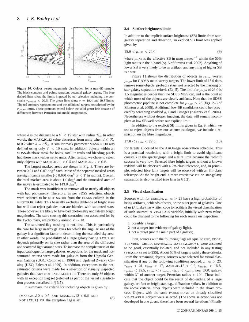
Including the near-IR selections increases the G12 target densitymarginally (to 1080 deg−2) while increasing the G09 and G15target density to720 deg−2. Figure 10 shows the colour biasfor the near-IR selections. Thez-band selection is complete to(r − z)model < 2.3 at the faint limit, while theK-band selec-tion is complete tormodel − KAB,auto < 2.9 at the faint limit.A zmodel < 18.2 selection is formally missing 0.3% of objectsbecause of thermodel limit, while a KAB,auto < 17.6 selectionis formally missing about 1% of objects. This is after applyingstar-galaxy separation. However, only very red objects aremissed,which are more likely to be stars in spite of the star-galaxy sepa-ration or have incorrectly measured colours caused by mismatchedapertures in the case ofr − K (the practical impact of these jointlimits is discussed later in§ 5.4). See also Fig. 4, ther < 20.5limit only makes an obvious impact in the galaxy number counts atKAB,auto > 17.8 that is above our selection limit.

3.3 Masking

In order to avoid targeting galaxies with bad photometry becausethey are near bright stars or satellite trails, an explicit mask wasconstructed. The bright-stars mask was based on stars down toV <12 in the Tycho 2, Tycho 1 and Hipparcos catalogues. For each star,a scattered-light radius (Rs) was estimated based on the circularregion over which the star flux per pixel is greater than 5 times thesky noise level. For each potential target, a mask parameterwasdefined as follows

MASK IC 12 = 1MASK IC 12 = Rs/dMASK IC 12 = 0

ford 6 Rs

Rs < d 6 5Rs

d > 5Rs

(7)

c© 2009 RAS, MNRAS000, 1–15

8 I. K. Baldry et al.

Figure 10. Colour versus magnitude distribution for a near-IR sample.The black contours and points represent potential galaxy targets. The bluedashed lines show the limits imposed by our selection including the con-straintrmodel < 20.5. The green lines showr = 19.4 and 19.8 limits.The red contours represent most of the additional targets not selected by therpetro limits. These contours extend below the solid green line because ofdifferences between Petrosian and model magnitudes.

whered is the distance to aV < 12 star with radiusRs. In otherwords, theMASK IC 12 value decreases from unity whend 6 Rs

to 0.2 whend = 5Rs. A similar mask parameterMASK IC 10 wasdefined using onlyV < 10 stars. In addition, objects within anSDSS-database mask for holes, satellite trails and bleeding pixelshad these mask values set to unity. After testing, we chose toselectonly objects withMASK IC 10< 0.5 andMASK IC 12< 0.8.

The largest masked areas are shown in Fig. 3. These are be-tween 0.01 and0.07 deg2 each. Most of the separate masked areasare significantly smaller (< 0.001 deg2 or< 1′ in radius). Overall,the total masked area is about1.0 deg2 and the unmasked area ofthe survey is estimated to be143.0 deg2.

The mask was insufficient to remove all or nearly all objectswith bad photometry. Therefore, as per SDSS selection, objectswere selected to beNOT SATUR from the FLAGS column in thePHOTOOBJ table. This basically excludes deblends of bright starsbut will also reject galaxies that are blended with saturated stars.These however are likely to have bad photometry and falsely brightmagnitudes. The stars causing this saturation, not accounted for bythe Tycho mask, are probably aroundV ∼ 13.

The saturated-flag masking is not ideal. This is particularlythe case for large nearby galaxies for which the angular sizeof thegalaxy is a significant factor in determining the excluded sky area.In other words, the probability of a large galaxy havingSATUR setdepends primarily on its size rather than the area of the diffractedand scattered light around stars. To increase the completeness of theinput catalogue for large galaxies, exceptions for the maskand not-saturated criteria were made for galaxies from the Uppsala Gen-eral Catalog (UGC; Cotton et al. 1999) and Updated Zwicky Cat-alog (UZC; Falco et al. 1999). In addition, exceptions to thenot-saturated criteria were made for a selection of visually inspectedgalaxies that haveNOT SATUR CENTER. There are only 86 objectswith an exception flag set (selected as part of the visual classifica-tion process described in§ 3.5).

In summary, the criteria for including objects is given by:

(MASK IC 10< 0.5 AND MASK IC 12 < 0.8 AND

NOT SATUR) OR the exception flag is set.(8)

3.4 Surface brightness limits

In addition to the implicit surface brightness (SB) limits from star-galaxy separation and detection, an explicit SB limit was appliedgiven by

15.0 < µr,50 < 26.0 (9)

whereµr,50 is the effective SB inmag arcsec−2 within the 50%light radius in ther-band (eq. 5 of Strauss et al. 2002). Anything oflower SB is very likely to be an artifact, and anything of higher SBis a star.

Figure 11 shows the distribution of objects inrfibre versusµr,50 for GAMA main-survey targets. The lower limit of 15.0 doesremove some objects, probably stars, not rejected by the masking orstar-galaxy separation criteria (Eq. 5). The limit forµr,50 of 26.0 is1.5 magnitudes deeper than the SDSS MGS cut, and is the point atwhich most of the objects are clearly artifacts. Note that the SDSSphotometric pipeline is not complete forµr,50 > 23 (figs. 2–3 ofBlanton et al. 2005). Additional low-SB candidates could berecov-ered by searching coaddedg, r andi images (Kniazev et al. 2004).Nevertheless without deeper imaging, the data will remain incom-plete at low SB well before our explicit limit.

In addition to the explicit SB limits given in Eq. 9, which weuse to reject objects from our science catalogue, we includea re-striction on the fibre magnitudes:

17.0 < rfibre < 22.5 (10)

for targets allocated to the AAOmega observation schedule.Thisis a practical restriction, with a bright limit to avoid significantcrosstalk in the spectrograph and a faint limit because the redshiftsuccess is very low. Selected fibre bright targets without a knownredshift will be observed with a 2m-class telescope, and, inprinci-ple, selected fibre faint targets will be observed with an 8m-classtelescope. At the bright end, a more restrictive cut on star-galaxyseparation is also justified (see later in§ 5.2).

3.5 Visual classification

Sources with, for example,µr,50 > 23 have a high probability ofbeing artifacts, deblends of stars, or the outer parts of galaxies. Oneof us (J. Liske) has written code to facilitate the visual classificationof such sources. AVIS CLASS variable, initially with zero value,could be changed to the following for each source on inspection:

1 possibly a target,2 not a target (no evidence of galaxy light),3 not a target (not the main part of a galaxy).

First, sources with the following flags all equal to zero,EDGE,BLENDED, CHILD , MAYBE CR, MAYBE EGHOST, were assumedto be good, essentially isolated, and not included in any testing(VIS CLASSset to 255). About 50% of targets satisfy these criteria.From the remaining objects, sources were selected for visual clas-sification if any of the following conditions applied:µr,50 > 23,rfibre > 21, rfibre < 17, MASK IC 12 > 0.2, rmodel < 15.5,rpetro < 15.5, rfibre < rmodel, rfibre < rpetro, near UGC galaxy,within 3′′ of another target, Petrosian radius> 10′′. These indi-cate that the object could be the result of deblending of a largegalaxy, artifact or bright star, e.g., diffraction spikes.In addition tothe above criteria, other objects were included in the abovepro-cess. Objects with the samePARENTID as an already classifiedVIS CLASS = 3 object were selected. (The above selection was notdeveloped in one go and there have been several iterations.)Finally

c© 2009 RAS, MNRAS000, 1–15

GAMA: The input catalogue and star-galaxy separation9

Figure 11.Bivariate distribution ofrfibre versusµr,50. The black contours and points represent objects that are not masked and pass star-galaxy separation.The grey lines outline the selection limits:15.0 < µr,50 < 26.0 is the restriction for the science catalogue; while objectswith fibre magnitudes fainterthan 22.5 or brighter than 17.0 are not included in the AAOmega observation schedule. The green dots represent objects with VIS CLASS=1; the red crossesVIS CLASS=2, and the pink crossesVIS CLASS=3. The small red circles atrfibre < 17 are probably stars based on a stricter star-galaxy separation criteria(§ 5.2). The blue dash-dotted (dashed) line corresponds to 50%(30%) redshift success rate for objects on or near the line.

objects, with the samePARENTID, that are the brightest and near-est to any object to be tested were included. Objects that could bepart of the same galaxy were viewed together where possible.Onehad to be certain to classify objects as 3 only if the main partwasidentified as a target.

The above selection produced a sample of about 12 500 ob-jects for visual classification, by six observers. Every selected ob-ject was classified by three different observers. Of the selected po-tential main-survey targets (Fig. 11),VIS CLASS=1 was set in 92%of cases,VIS CLASS=2 in 5% of cases, andVIS CLASS=3 in 3% ofcases, based on agreement between two or all three classifiers, 9%and 90% of cases, respectively. Some of the ambiguous cases weredouble checked, and a single-observer classification was selectedin 1% of cases. Objects with values of 2 or 3 were removed fromthe schedule of AAT observations, i.e., targets must satisfy

VIS CLASS 6= 2 AND VIS CLASS 6= 3 . (11)

In addition, theVIS CLASS= 3 objects can be used to improve thephotometry of some large galaxies by coadding in the flux of thegalaxy parts (or the ‘parent’ photometry can be used).

3.6 Number of targets

The total number of objects that are within the GAMA regions(§ 2.1), main-survey magnitude limits (Eq. 6) and∆sg > 0.05,

is 143 728. Applying the stricter star-galaxy separation (Eq. 5) re-duces the sample to 132 073. Removing objects by masking (Eq.8),the SB limits (Eq. 9) and visual checking (Eq. 11), reduces the sam-ple to 120 038. Of these, 825 were not included in the AAOmegaobservation schedule because they do not satisfy the fibre magni-tude limits (Eq. 10). A more restictive star-galaxy separation can beapplied for brighter targets (discussed later and given in Eq. 12) thatreduces the sample to119 852. This is considered to be the main-survey sample. Note these numbers apply to AAT observationsin2009, the numbers may change slightly with addition of completeJ-K UKIDSS.

Separating the main survey intor, z and K limited sam-ples, the numbers are 114 520, 61 418 and 57 657, respectively.For rpetro selected samples to 19.0, 19.4 and 19.8, the samplesizes are 60 407, 96 386 and 150 810, respectively. The latteris ther-selected main survey plus F2 additional targets, which arede-scribed in the following section.

3.7 Additional targets

In order to assess the spectro-photometry of the AAOmega spec-tra, three or four stars, classified asREDDEN STD or SPEC-TROPHOTOSTD by SDSS, were observed in each configuration.These also had a bright fibre magnitude limit of 17 as per the main-survey targets.

The aim is to obtain high completeness (99%), at least in terms

c© 2009 RAS, MNRAS000, 1–15

10 I. K. Baldry et al.

of spectra obtained and ideally in terms of confirmed redshifts, forthe main survey. This is set to reduce systematic uncertainties inGAMA’s position dependent science cases, and is possible becausea given patch of sky is potentially observed by∼ 5–10 2dF tilesdepending on the local density of targets (see Robotham et al. 2009for a description of the tiling strategy). Given this requirement, tar-geting becomes increasingly inefficient as the survey progresses(fewer targets without a redshift per tile). Filler targetswere in-troduced to provide useful redshifts outside the main survey, andthus, maximise fibre usage. These have no high-level requirementon completeness. The filler selections are given by: (F1) objectswith detection in the Faint Images of the Radio Sky at Twenty-cm(FIRST) survey and matched to SDSS withimodel < 20.5 includ-ing unresolved sources; (F2)19.4 < rpetro < 19.8 galaxy tar-gets in G09 and G15, aiming for equal depth with G12; and (F3)gmodel < 20.6 or rmodel < 19.8 or imodel < 19.4 in G12, investi-gating variation in magnitude-type and wavelength on selection. Intotal, there are about 50 000 filler targets.

4 SPECTROSCOPY

4.1 Existing data sets

While the GAMA target density is significantly higher than SDSSor 2dFGRS, the redshifts obtained by these and other surveyspro-vide a non-negligible starting baseline. We incorporate a number ofdifferent surveys into our catalogue, defining a redshift quality Q,where necessary, as per the Colless et al. (2001) scheme suchthatQ = 1 means very poor or no redshift,Q = 2 means a possible butdoubtful redshift,Q = 3 means a probable redshift, andQ = 4 orQ = 5 means a reliable redshift. The surveys included are given inTable 3.

From theQ > 3 non-GAMA redshifts in the GAMA re-gions as outlined in the table, about 40 000 are unique (consideringmatches within1′′ to be the same object). The number of main sur-vey targets with one of these redshifts is 19 446, matching within1′′

except for some large galaxies within3′′ of a 6dFGS or UZC red-shift. The non-GAMA redshifts without a match to a GAMA targetare primarily of stars and quasars. Objects withQ > 3 redshifts aregiven a lower priority in the AAOmega observation schedule.

4.2 AAOmega observations in 2008 and 2009

GAMA observations with the multi-object spectrograph AAOmegaon the AAT took place in 2008 (Jan 12, Feb 29 to Mar 15, Mar 30to Apr 05) and 2009 (Feb 27 to Mar 05, Mar 27 to Apr 02, Apr 17 toApr 23). The 2dF robotic fibre positioner (Lewis et al. 2002) feedsa bench-mounted dual-beam spectrograph (Sharp et al. 2006). Twoplates are used: while one is being configured (fibres placed), theother plate is in the focal plane feeding light to the spectrograph.There are up to 392 science fibres available in a single configu-ration. Excluding broken fibres, 20–25 fibres used for sky subtrac-tion and 3 or 4 spectroscopic standards (§ 3.7), we targeted between320 and 350 GAMA targets per configuration. Total exposure timesused were typically 1 hour (3× 20min). We observed up to 8 con-figurations in a single night for a total of 267 observations over thetwo years (91 015 spectra). The spectral coverage was from 370 to880 nm.

The priorities assigned to targets were different betweenthe two years. The tiling scheme is described in detail byRobotham et al. (2009). Here, we summarize the priorities. In 2008

Table 4.GAMA spectra from AAT observations in 2008 and 2009

description number

total spectra obtained 91015spectroscopic standards 1059unique targets 87753repeated targets 2203

Q > 3 unique targetsa 82696r < 19.0 & ∆sg > 0.25 40103main surveyr-selected 38994main surveyz,K-selected 1847F1: radio selected 105F2:19.4 < r < 19.8 in G09 & G15 1029F3: filler selection in G12 68otherb 550

aThe unique targets with redshifts are identified in the rows below. Ther < 19.0 selection corresponds to the higher priority targets in thefirstyear of AAT observations. The numbers shown in each row belowthis rowdo not include contributions already accounted for. Below the main surveyare the F1–F3 filler targets (§ 3.7).bThe ‘other’ objects are mostly objects whose UKIDSS photometry hasundergone revision since the second year of AAT observations, andVIS CLASS=3 objects that were observed prior to implementation of thevisual classification.

the targets consisted only of ther-band selection with∆sg > 0.25(there was insufficient UKIDSS coverage at the time), withoutan already known redshift (§ 4.1) except for some cross-checkdata. The priorities were from high-to-low: (i)r < 19.0; (ii)19.0 < r < 19.8 in G12 within±0.5◦ of the celestial equator; (iii)19.0 < r < 19.4 in G09 and G15, and remaining19.0 < r < 19.8in G12. In addition, clustered targets in any of these categories weregiven a higher priority. A clustered target was defined as onewithin40′′ of another target, where40′′ is approximately the closest twofibres can be placed. This was to maximise the chances of observ-ing as many close pairs as possible over three years of observations.In 2009, now including UKIDSS selection for the star-galaxysep-aration and magnitude limits, the priorities were: (i) clustered un-observed main-survey targets; (ii) unobserved main surveyor clus-tered failed main survey, where failed means that a GAMA spec-trum has been obtained withQ 6 2; (iii) failed main survey; (iv)from F1, F2, F3 filler targets, andQ = 3 spectra taken with the old2dF spectrographs (e.g., 2dFGRS).

From the first two years of observing, first-pass reductionswith 2DFDR (Croom et al. 2004) andRUNZ (Saunders et al. 2004)have resulted in a 94 per cent redshift success rate (Q > 3) for82 696 unique redshifts, 80 944 for the main survey (79 599 withz > 0.002). Table 4 gives a breakdown of the spectra obtained. In-cluding spectra from other surveys, results in 100 012Q > 3 red-shifts for the main survey (98 497 withz > 0.002). Table 5 givesthe target numbers and redshift completeness for various main sur-vey selections. Note particularly the drop in completenessbetweenrpetro < 19.0 (96% average completeness) and the fainterr-bandselection (74%), and a further drop to thez- andK-band extra se-lection (39%). Ther-limit only selection and the prioritisation inthe first year is the main cause of differingQ > 3 completenessfactors between each sub-sample, i.e., it is primarily a variation intargeting completeness though redshift success rate is also lowerfor the fainter samples. No observations based onJ and/orK-bandphotometry were started in the first year so the marginally resolvedsample within each magnitude range is also of lower completeness.

c© 2009 RAS, MNRAS000, 1–15

GAMA: The input catalogue and star-galaxy separation11

Table 3.Other spectroscopic data in the GAMA regions. Tables were obtained from the survey websites or the VizieR service.

survey file/table reference no. of redshiftsa no.Q > 3 no. main survey uniqueb

SDSS DR7SPECOBJALL Abazajian et al. (2009) 27514 26687c 131702dFGRS VII/250/2dfgrs Colless et al. (2003) 11490 11180 3840MGCz VII/240/mgczcat Driver et al. (2005) 4008 3835 18832SLAQ-LRG J/MNRAS/372/425/catalog Cannon et al. (2006) 2256 2109 2276dFGS DR3SPECTRA Jones et al. (2009) 299 270 55UZC J/PASP/111/438/catalog Falco et al. (1999) 255 209d 132QZ VII/241/2qz Croom et al. (2004) 5359 4317e 2242SLAQ-QSO 2slaqqso public.cat Croom et al. (2009) 2414 2098e 34

aThe number of redshifts quoted are all those in the GAMA regions including duplicates and non-GAMA targets.bThe number corresponds to unique main survey targets with aQ > 3 redshift from the survey (prior to GAMA). In the case of multiple matches within1′′,the highestQ value match is used (nearest in case of equalQ): Q is limited to6 4 for all surveys except SDSS.cSDSS quality is given byQ = 1 + (ZCONF> 0.2) + (zwarningokayAND ZCONF > 0.7) + (ZCONF> 0.9) + (ZCONF> 0.99) where each term inbrackets takes the value of unity if the condition is true andzero otherwise, and zwarningokay takes the value unity if the following warning flagsEMAB INC, AB INC, 4000BREAK are all zero.dUZC quality is given by:Q = 3 if UZC class is 0 or 1 (secure identification), andQ = 2 if UZC class is 2, 3 or 4 (some confusion regarding identification).e2QZ and 2SLAQ-QSO quality is given by:Q = 3 if original quality code was 11 (good identification and redshift); Q = 2 if 22, 12 or 21; andQ = 1 if 33,23 or 32.

Table 5. Main survey target numbers and redshift completeness for the three separate GAMA regions, galaxy fractions (fromQ > 3 redshifts), and mediangalaxy redshifts. The redshift completeness is defined as the number of objects with aQ > 3 redshift divided by the number of targets (regardless of whetherthey have been observed spectroscopically).

selection Region G09 Region G12 Region G15 fraction medianno. targets Q > 3 no. targets Q > 3 no. targets Q > 3 z > 0.002 redshift

rpetro < 16.0 363 95.0% 397 97.5% 481 96.9% 99.1% 0.05216.0 < rpetro < 17.8 3335 99.2% 4644 99.3% 4666 99.0% 98.5% 0.11617.8 < rpetro < 19.0 & ∆sg > 0.25 14387 98.2% 15599 96.1% 16016 93.1% 99.0% 0.18517.8 < rpetro < 19.0 & ∆sg < 0.25 160 83.8% 206 60.7% 153 55.6% 66.3% 0.26019.0 < rpetro < 19.4 & ∆sg > 0.25 11886 90.6% 11600 76.4% 11724 62.6% 98.9% 0.24319.0 < rpetro < 19.4 & ∆sg < 0.25 201 77.1% 345 46.1% 223 33.6% 80.7% 0.22819.4 < rpetro < 19.8 & ∆sg > 0.25 — — 17281 70.1% — — 99.5% 0.26319.4 < rpetro < 19.8 & ∆sg < 0.25 — — 853 38.9% — — 93.7% 0.254zmodel < 18.2 and notr-selected 604 63.1% 270 25.2% 510 38.2% 58.4% 0.470KAB,auto < 17.6 and notrz-selected 1931 46.5% 348 19.0% 1669 29.5% 97.3% 0.368

all main survey 32867 91.6% 51543 80.9% 35442 79.5% 98.5% 0.196

The details of spectroscopic data reduction, including newde-fringing and sky-subtraction techniques, redshifting, comparisonwith other spectra, spatial and magnitude completeness will be de-scribed in future GAMA papers. In the next section, we use thefirst-pass redshifts to illustrate some issues related to the target se-lection.

5 RESULTS

5.1 Star-galaxy separation

There are two star-galaxy separation parameters used in theGAMAselection. Figure 12(a) shows the observed bivariate distribution ofmain survey targets in these parameters. The red line shows the cutused for our target selection. This removes nearly 9 000 sourcesor about 7% of potential targets to∆sg > 0.05. Figure 12(b,c)show the distributions of galaxies (z > 0.002) and stars that haveconfirmed redshifts, 1.5% are stellar, using all available spectro-scopic data. The additionalJ − K selection was necessary for

sources withr > 17.8 in order to be complete for compact galax-ies. This is seen by the confirmed galaxy contours extending to theleft of ∆sg = 0.25 in Fig. 12(b), which would otherwise have beenmissed by using only a∆sg > 0.25 cut. Note that the targetingcompleteness is lower at∆sg < 0.25, 60% compared to nearly90% overall, because this UKIDSS-SDSS selection was not avail-able for AAT observations in 2008.

Figure 12 also shows that the regions of high stellar contami-nation are, not surprisingly, at low∆sg or∆sg,jk. Thus a lower con-tamination could be obtained by using a cut∆sg+∆sg,jk > 0.4, forexample, with minimal rejection of genuine galaxies. This wouldwork well because there is no strong correlation between thetwoparameters.

An estimate of the completeness of the current selection interms of selecting galaxies can be obtained by assuming thatthereis no significant correlation between∆sg and ∆sg,jk. Considerthe galaxy distribution in Fig. 12(b). The fraction of galaxies at∆sg,jk < 0.2 is 2.3% (not including galaxies with noJ −K mea-surement) and the fraction at∆sg < 0.25 is 1.7% after adjustingthe latter for the lower targeting completeness. Thus the predicted

c© 2009 RAS, MNRAS000, 1–15

12 I. K. Baldry et al.

Figure 12.Results of star-galaxy separation.(a): The distribution of main survey targets with aJ−K measurement, extended to all objects with∆sg > 0.05,are shown with black contours and points. The red dashed lineshows the cut used for target selection.(b,c): The distribution of objects (rpetro > 17.8, < 17.8)with confirmed galaxy redshifts are shown with green contours and points, while objects with stellar redshifts are shownwith red points. The blue dotted (dash-dotted) line corresponds to 50% (70%) stellar contamination for objects on or near the line (determined by interpolation in ther < 17.8 sample).(d): Objectswith rfibre < 17.0, not included in the AAOmega observation schedule, are shown. Red crosses and green diamonds represent objects with confirmed stellarand galaxy redshifts. Black crosses (squares) represent objects where the fibre magnitude is brighter (fainter) than the Petrosian magnitude. The smaller squaresand crosses are the potential targets excluded by the criteria of Eq. 12: these are also shown as small red circles in Fig. 11. The blue dashed line divides thesmall and large squares.

fraction of galaxies at∆sg,jk < 0.2 and∆sg < 0.25 (in the lower-left hand corner of the plot) is only 0.04%. Thus, the galaxy se-lection from the star-galaxy separation is plausibly& 99.9% com-plete when there areJ andK measurements. This assumes there isno significant population of galaxies with∆sg < 0.05 within ourmagnitude limits.

The SDSS pipelinePHOTO also determines the scale radiiof the de Vaucouleurs and exponential profile fits (eq. 9 & 10 ofStoughton et al. 2002). Taking the best fit and averaging the scaleradii in ther- andi-bands for each galaxy, we determined the com-pleteness in this measure of size. The cut∆sg > 0.25 is completedown to a scale radius∼ 0.6′′, while our star-galaxy separation(Eq. 5) is plausibly complete down to a scale radius∼ 0.25′′.5

Figure 13 shows the scale radius in kpc versus redshift for con-firmed galaxies in the main survey. Without the additional selec-

5 We note that thePHOTO scale radius values should be interpretedwith some caution at small sizes, less than half the typical PSF width.Taylor et al. (2009) advocate treating objects with scale radii < 0.75′′ ashaving an upper limit of0.75′′, i.e., the true value is poorly determinedeven thoughPHOTOhas determined that the object is likely to be resolved.

tion, the target selection would be significantly incomplete,∼ 20%missed, for galaxies with observed radii between0.25′′ and0.6′′.Of course, one could have used this scale radius directly as astar-galaxy separation parameter but, without higher resolution imag-ing, the systematic errors are presumably larger in this than∆sg.

This compact galaxy selection is critical for studies with adi-rect interest in the size evolution of galaxies (e.g., Trujillo et al.2006; Cameron & Driver 2007; Taylor et al. 2009). Targeting allobjects with∆sg > 0.05 would have resulted in∼ 9 000 extraobjects, which would have been a very inefficient way to targetcompact galaxies. Future higher S/N and higher resolution imag-ing (optical and near-IR) will improve the efficiency of thistype ofselection, providing a test of whether GAMA target selection hasmissed significant numbers of compact galaxies.

5.2 Bright galaxies

Objects withrfibre < 17.0 are not allocated to the AAOmegaschedule to avoid crosstalk between spectra tramlines, andwe donot need to consider these objects for this target selection. How-ever, it is necessary for analyses at low redshift, e.g. measuring lu-

c© 2009 RAS, MNRAS000, 1–15

GAMA: The input catalogue and star-galaxy separation13

Figure 13.Scale radius, de Vaucouleurs or exponential profile fromPHOTO,versus redshift. The black contours and points represent galaxies selectedusing∆sg > 0.25, while red crosses represent theJ − K selected sam-ple with 0.05 < ∆sg < 0.25. The dashed lines correspond to constantobserved angular size.

minosity functions, to determine a realistic completenessof galaxyselection at bright magnitudes. Figure 12(d) shows the distributionin the star-galaxy separation parameters for these potential targets.There are 485 using our normal selection criteria, of which,296have redshifts from SDSS and other surveys (Q > 3; Table 3). Onepossibility would be to observe all remaining 189 targets with a2m-class telescope. However, most of these are probably stars anda more restrictive criterion could be used. This is given by

rfibre > 17.0 OR

(∆sg +∆sg,jk > 0.6 OR ∆sg > 0.6 AND

rfibre > rpetro) .(12)

The∆sg-∆sg,jk cut is shown by the blue dashed line in Fig. 12(d),while targets that satisfy the last criteria are shown as squares asopposed to crosses. Sources with fibre magnitude brighter than Pet-rosian are indicative of a ‘possible’ galaxy blended with a star,however, the star light dominates the fibre magnitude, whichis notdeblended. Using the above cut results in 299 sources with 266redshifts (89% complete). This cut should be used when assessingcompleteness at the bright end of GAMA targets. This was appliedbefore computing therpetro < 16 target numbers and complete-ness given in Table 5.

5.3 Low surface brightness galaxies

The completeness in the low SB regime depends on redshift suc-cess and source detection (Disney & Phillipps 1983; Blantonet al.2005), and there is the additional issue of the accuracy of the fluxmeasurements (Cameron & Driver 2007). These will be describedin detail in a future paper on luminosity functions (Lovedayet al.in preparation). Here we note only that the redshift successrate isprimarily a function ofrfibre as shown in Fig. 11. The success rateis 50% atrfibre ∼ 21.5. This does not include any coadding ofGAMA spectra over two or more observations, and there may beimprovement after re-reduction.

Figure 14. Redshift distributions for selected main-survey samples.Thenumbers have been projected to completion of the main surveyusing em-pirical completeness determined ing − i bins.

5.4 Redshift distributions and near-IR selections

Not accounting for incompleteness, 50% of the galaxy redshifts arein the range 0.13–0.27, 90% are in the range 0.06–0.39 and 99%arein the range 0.02–0.53. Figure 14 shows the redshift histograms forvarious galaxy samples (z > 0.002) within the main survey, andmedian redshifts are given in Table 5. The near-IR selections havea higher average redshift. Note that the redshift distribution withineach sub-sample may be biased by non-GAMA redshifts and thedependence of redshift success rate on magnitude, for example.These are corrected for in Fig. 14 by binning ing − i to deter-mine completeness factors. The histogram for each sub-sample isdetermined by weighting each object with a redshift by1/c wherec is the redshift completeness in each bin (with bin size of 0.2for0 < g − i < 3). This colour is used because of its correlation withredshift [Fig. 6(b)].

Figure 15(a) shows observedr − z versus redshift for thez-selected sample, with the targets fainter than 19.4 inr shown byred points. The extraz-band selection is mostly picking up lumi-nous galaxies in the redshift range 0.4–0.6 (recalling thatthis isof lower completeness than ther < 19.4 selection). The num-ber density of targets drops off well before the colour bias limit.Simple stellar population (SSP) tracks are shown with a formationredshift of six (see caption for references). Some objects are appar-ently redder than the old SSP tracks. This is presumably mostly be-cause of photometric errors, however, certain dust geometries canin principle redden galaxies beyond the colour of old stellar pop-ulations. Dusty galaxies can lie on, and slightly redder than, thered sequence (Wolf et al. 2005). Note that most of the targetsin therange1.2 < r − z < 2.5 are a stellar contamination (or 41.6% ofthez-band extra selection, see Table 5).

Figure 15(b) shows observedrmodel − KAB,auto versus red-shift for theK-selected sample, with the targets fainter than 19.4 inr and 18.2 inz shown by red points. The extra selection is mostlypicking up red galaxies in the redshift range 0.2–0.5. The tracksshow that theK selection is possibly incomplete for maximally oldsuper-solar metallicity populations at redshift> 0.45 (from one ofthe models). There are many sources significantly redder than thetracks, however, this is most probably because of the mismatch inapertures between the surveys (model versusAUTO mags, different

c© 2009 RAS, MNRAS000, 1–15

14 I. K. Baldry et al.

Figure 15.Observed colour versus redshift for (a) thezmodel < 18.2 sam-ple and (b) theKAB,auto < 17.6 sample. The black contours and pointsrepresent the data withinrpetro < 19.4 (or zmodel < 18.2 for theK-selected sample), while the red points represent the remaining fainter se-lection. The dash-dotted lines represent the observed colours of SSP mod-els with zform = 6 (12.5 Gyr old atz = 0, 7.5 Gyr atz = 0.5): red(Z = 0.05, Bruzual & Charlot 2003), blue (Z = 0.04, alpha-enhancedabundances, Percival et al. 2009), and green (Z = 0.02, empirical stel-lar spectra, Maraston et al. 2009). The horizontal dashed line represents thecompleteness limit at the faint end of the samples given thermodel < 20.5limit (Fig. 10).

deblending algorithms). For most purposes, it would be adequateto assume the selection isK-band limited only.

6 SUMMARY

The GAMA survey is designed to be a highly complete redshiftsurvey with a target density several times that of SDSS. The sur-vey covers three48 deg2 regions near the celestial equator centredon 9 h, 12 h and 14.5 h (Fig. 2). The input catalogue is drawn fromthe SDSS and UKIDSS. The main-survey limits arerpetro < 19.4,zmodel < 18.2 andKAB,auto < 17.6 (K < 15.7) across all theregions, andrpetro < 19.8 over the G12 region (Eq. 6). This cor-responds to a main survey of 119 852 targets. The near-IR selec-tions have a joint constraint withrmodel < 20.5, which has min-imal impact on the use of the near-IR selections (Figs. 10 & 15).The GAMA survey lies between that of the SDSS-MGSr < 17.8and VVDS-wideIAB < 22.5 magnitude-limited samples in thedepth-area plane (Fig. 1). In terms ofK-band selection (Figs. 3& 4), GAMA covers an area∼ 15 times that of the similar-depthHawaii+AAOK < 15 survey.

In order to be highly complete at the high-SB end of the galaxydistribution, an intensity profile parameter (Eq. 1) and a colour-colour parameter (Eq. 2) are used jointly for star-galaxy separa-

tion. The∆sg,jk parameter makes use ofJ −K andg − i colours.Either parameter works reasonably well in separating starsandgalaxies (Figs. 5–8). A joint selection (Eq. 5) increases the com-pleteness while stellar contamination in the sample remains at lessthan 2%. Judging by the joint distribution of confirmed galaxies inthese parameters (Fig. 12), the completeness is high because thebivariate density drops significantly prior to the limit of our selec-tion. This is particularly important when considering the size evo-lution of galaxies (Fig. 13). The incompleteness at the low-SB endis significant, both in source detection and redshift success rate,which is about 50% atrfibre = 21.5 (Fig. 11). Some improvementover the SDSS MGS is made by visually checking low-SB targets(µr,50 > 23), rather than using automatic checks, by increased red-shift success rate, and by eventually including further integrationsof sources with failed redshifts.

The GAMA survey has completed two out of a three-year timeallocation for spectroscopy with AAOmega on the AAT. To date,100 012 redshifts have been confirmed for the main survey, includ-ing 80 944 from AAOmega. Of these, 98.5 per cent are extragalac-tic. The completeness is 96% forrpetro < 19.0, 74% for the fainterr-band selection, and∼ 39% for the remaining near-IR selection(Table 5). The completeness atr > 19 will be significantly im-proved in the third year of spectroscopic observations. We expectthat this galaxy redshift survey will form a core of a fundamentaldatabase for many studies in extragalactic astronomy.

ACKNOWLEDGEMENTS

This part of the GAMA survey has been made possible by the ef-forts of staff at the Anglo-Australian Observatory, and membersof the Sloan Digital Sky Survey and UKIRT Infrared Deep SkySurvey teams. We thank Steven Warren in particular for efforts inmaking the GAMA regions a high priority in UKIDSS, the anony-mous referee for useful suggestions, and Daniel Mortlock for dis-cussion regarding star-galaxy separation. Database and software re-sources used in this paper include the SDSS Catalog Archive ServerJobs (CASJobs) System, the UKIDSS WFCAM Science Archive(WSA), the VizieR catalogue service, the IDL Astronomy User’sLibrary, IDLUTILS , Astromatic software, and Starlink Tables In-frastructure Library Tool Set (STILTS). I. Baldry acknowledgesfunding from Science and Technology Facilities Council (STFC)and Higher Education Funding Council for England (HEFCE).

REFERENCES

Abazajian K., et al., 2004, AJ, 128, 502Abazajian K., et al., 2009, ApJS, 182, 543Adelman-McCarthy J. K., et al., 2006, ApJS, 162, 38Adelman-McCarthy J. K., et al., 2008, ApJS, 175, 297Berlind A. A., et al., 2006, ApJS, 167, 1Bertin E., Arnouts S., 1996, A&AS, 117, 393Bertin E., Mellier Y., Radovich M., Missonnier G., Didelon P.,

Morin B., 2002, in Bohlender D. A., Durand D., HandleyT. H., eds, ASP Conf. Ser., Vol. 281, ADASS XI. ASP, SanFrancisco, p. 228

Binggeli B., Sandage A., Tammann G. A., 1988, ARA&A, 26, 509Blanton M. R., et al., 2003, ApJ, 592, 819Blanton M. R., Lupton R. H., Schlegel D. J., Strauss M. A.,

Brinkmann J., Fukugita M., Loveday J., 2005, ApJ, 631, 208Bruzual G., Charlot S., 2003, MNRAS, 344, 1000

c© 2009 RAS, MNRAS000, 1–15

GAMA: The input catalogue and star-galaxy separation15

Cameron E., Driver S. P., 2007, MNRAS, 377, 523Cannon R., et al., 2006, MNRAS, 372, 425Carlberg R. G., Yee H. K. C., Ellingson E., Abraham R., GravelP.,

Morris S., Pritchet C. J., 1996, ApJ, 462, 32Casali M., et al., 2007, A&A, 467, 777Cole S., et al., 2001, MNRAS, 326, 255Colless M., et al., 2001, MNRAS, 328, 1039Colless M., et al., 2003, e-Print archive, arXiv:astro-ph/0306581Cotton W. D., Condon J. J., Arbizzani E., 1999, ApJS, 125, 409Croom S., Saunders W., Heald R., 2004, Anglo-Australian Obser.

Newsletter, 106, 12Croom S. M., et al., 2009, MNRAS, 392, 19Croom S. M., Smith R. J., Boyle B. J., Shanks T., Miller L., Outram

P. J., Loaring N. S., 2004, MNRAS, 349, 1397da Costa L. N., et al., 1998, AJ, 116, 1Davis M., et al., 2003, Proc. SPIE, 4834, 161Davis M., Geller M. J., Huchra J., 1978, ApJ, 221, 1Davis M., Huchra J., Latham D. W., Tonry J., 1982, ApJ, 253, 423de Lapparent V., Geller M. J., Huchra J. P., 1988, ApJ, 332, 44De Propris R., Liske J., Driver S. P., Allen P. D., Cross N. J. G.,

2005, AJ, 130, 1516Disney M., Phillipps S., 1983, MNRAS, 205, 1253Drinkwater M. J., et al., 2009, MNRAS, in press (arXiv:0911.4246)Driver S. P., et al., 2009, Astron. Geophys., 50, 5.12Driver S. P., Liske J., Cross N. J. G., De Propris R., Allen P. D.,

2005, MNRAS, 360, 81Dye S., et al., 2006, MNRAS, 372, 1227Eisenstein D. J., et al., 2001, AJ, 122, 2267Eke V. R., Baugh C. M., Cole S., Frenk C. S., Navarro J. F., 2006,

MNRAS, 370, 1147Eke V. R., et al., 2004, MNRAS, 348, 866Ellis R. S., Colless M., Broadhurst T., Heyl J., Glazebrook K.,

1996, MNRAS, 280, 235Elston R. J., et al., 2006, ApJ, 639, 816Erdogdu P., et al., 2006, MNRAS, 368, 1515Falco E. E., et al., 1999, PASP, 111, 438Fukugita M., Ichikawa T., Gunn J. E., Doi M., Shimasaku K.,

Schneider D. P., 1996, AJ, 111, 1748Garilli B., et al., 2008, A&A, 486, 683Gunn J. E., et al., 1998, AJ, 116, 3040Hambly N. C., et al., 2008, MNRAS, 384, 637Hewett P. C., Warren S. J., Leggett S. K., Hodgkin S. T., 2006,

MNRAS, 367, 454Hodgkin S. T., Irwin M. J., Hewett P. C., Warren S. J., 2009, MN-

RAS, 394, 675Hogg D. W., Finkbeiner D. P., Schlegel D. J., Gunn J. E., 2001,AJ,

122, 2129Huang J.-S., Glazebrook K., Cowie L. L., Tinney C., 2003, ApJ,

584, 203Huchra J. P., Geller M. J., 1982, ApJ, 257, 423Ivezic Z., et al., 2002, in Green R. F., Khachikian E. Y., Sanders

D. B., eds, ASP Conf. Series, Vol. 284, AGN Surveys. ASP,San Francisco, p. 137

Jarrett T. H., Chester T., Cutri R., Schneider S., SkrutskieM.,Huchra J. P., 2000, AJ, 119, 2498

Jarrett T. H., et al., 2010, AJ, submittedJones D. H., et al., 2009, MNRAS, 399, 683Kniazev A. Y., Grebel E. K., Pustilnik S. A., Pramskij A. G., Kni-

azeva T. F., Prada F., Harbeck D., 2004, AJ, 127, 704Kron R. G., 1980, ApJS, 43, 305Lawrence A., et al., 2007, MNRAS, 379, 1599Le Fevre O., et al., 2005, A&A, 439, 845

Lewis I. J., et al., 2002, MNRAS, 333, 279Lilly S. J., et al., 2007, ApJS, 172, 70Lilly S. J., Le Fevre O., Crampton D., Hammer F., Tresse L., 1995,

ApJ, 455, 50Liske J., Lemon D. J., Driver S. P., Cross N. J. G., Couch W. J.,

2003, MNRAS, 344, 307Loveday J., Peterson B. A., Efstathiou G., Maddox S. J., 1992, ApJ,

390, 338MacGillivray H. T., Martin R., Pratt N. M., Reddish V. C., Seddon

H., Alexander L. W. G., Walker G. S., Williams P. R., 1976,MNRAS, 176, 265

Maddox S. J., Efstathiou G., Sutherland W. J., Loveday J., 1990,MNRAS, 243, 692

Maraston C., Stromback G., Thomas D., Wake D. A., Nichol R.C.,2009, MNRAS, 394, L107

Moore B., Frenk C. S., White S. D. M., 1993, MNRAS, 261, 827Norberg P., et al., 2002a, MNRAS, 336, 907Norberg P., et al., 2002b, MNRAS, 332, 827Padmanabhan N., et al., 2008, ApJ, 674, 1217Percival S. M., Salaris M., Cassisi S., Pietrinferni A., 2009, ApJ,

690, 427Peterson B. A., Ellis R. S., Efstathiou G., Shanks T., Bean A.J.,

Fong R., Zen-Long Z., 1986, MNRAS, 221, 233Ratcliffe A., Shanks T., Broadbent A., Parker Q. A., Watson F. G.,

Oates A. P., Fong R., Collins C. A., 1996, MNRAS, 281, L47Robotham A., et al., 2009, Publ. Astron. Soc. Australia, in press

(arXiv:0910.5121)Saunders W., Cannon R., Sutherland W., 2004, Anglo-Australian

Obser. Newsletter, 106, 16Saunders W., et al., 2000, MNRAS, 317, 55Saunders W., Rowan-Robinson M., Lawrence A., Efstathiou G.,

Kaiser N., Ellis R. S., Frenk C. S., 1990, MNRAS, 242, 318Schechter P., 1976, ApJ, 203, 297Schlegel D. J., Finkbeiner D. P., Davis M., 1998, ApJ, 500, 525Sharp R., et al., 2006, Proc. SPIE, 6269, 62690GShectman S. A., Landy S. D., Oemler A., Tucker D. L., Lin H.,

Kirshner R. P., Schechter P. L., 1996, ApJ, 470, 172Skrutskie M. F., et al., 2006, AJ, 131, 1163Smith J. A., et al., 2002, AJ, 123, 2121Steidel C. C., Adelberger K. L., Shapley A. E., Pettini M., Dickin-

son M., Giavalisco M., 2003, ApJ, 592, 728Stoughton C., et al., 2002, AJ, 123, 485Strauss M. A., et al., 2002, AJ, 124, 1810Taylor E. N., Franx M., Glazebrook K., Brinchmann J., van

der Wel A., van Dokkum P. G., 2009, ApJ, submitted(arXiv:0907.4766)

Taylor M. B., 2005, in Shopbell P., Britton M., Ebert R., eds,ASPConf. Ser., Vol. 347, ADASS XIV. ASP, San Francisco, p. 29

Trujillo I., et al., 2006, ApJ, 650, 18Vettolani G., et al., 1997, A&A, 325, 954Warren S. J., et al., 2007, MNRAS, 375, 213Watson C. R., et al., 2009, ApJ, 696, 2206Wolf C., Gray M. E., Meisenheimer K., 2005, A&A, 443, 435Yee H. K. C., et al., 2000, ApJS, 129, 475York D. G., et al., 2000, AJ, 120, 1579Zehavi I., et al., 2005, ApJ, 630, 1Zwicky F., 1937, ApJ, 86, 217

c© 2009 RAS, MNRAS000, 1–15