Exotic Beam Summer School @ MSU

EBSS3, 7/23/2015

Gamma-ray Tracking++ The Compton suppressed arrays

The tracking arrays

Traces and decomposition

Clustering and tracking

Efficiency of tracking arrays

Tracking efficiency and P/T

Data quality issues

Challenges and future

Torben Lauritsen, ANL

for the GRETINA collaboration

torben@anl.gov

2

The Compton suppressed arrays

GAMMASPHERE 110/100 modules

Idea:

Suppress gamma rays that

scattered out of the germanium

crystal with highly efficient BGO

detectors surrounding the crystal on all

sides. Can 'honeycomb suppress' as

well.

Works very well, but ~60% of the array

is taken up by the BGO detectors.

Fundamentally, we can't improve the

Compton suppressed arrays!!

For Gammasphere, the Doppler

correction cannot be done better than

to ½ the opening angle of the ge

crystals (for split crystals at 90 deg) Germanium

BGO

3

The new advent,

The tracking arrays (GRETINA and AGATA)

GRETINA module, 30/9 modules or

120/36 crystals from Canberra Eurisis

(now Mirion)

Idea:

Replace the BGO with

active segmented

germanium crystals

But the data analysis becomes

quite a bit more complicated.

The efficiency can be about 4

times that of GAMMASPHERE

and the gamma ray position

resolution can be done with a

precision of 2-3 mm (rms)

module Crystals x4, two types

36 segments

Canberra EurysisCanberra Eurysis

AGATA: 180 crystals,

3 per cryostat, 3 types

4

The signals from the traces:

(from D. C. Radford)

Net

charge

Induced chargeInduced charge

Central

contact

trace

Key to understanding tracking arrays:

5

Each segment signal feed to a 14 bit FLASH ADC (100 MHz)

Basic Idea:

The digital traces fromthe segments will determine the (x,y,z) and interactionenergies at the Interaction points

10x4 channels eachCC also digitized

[same as DGS/DFMA !!]

6X6=36 + few CC signals

We get complete TRACES

Trigger

Mods

(ANL)

VME IOC

MVME

5500

Digitizers

40 channels

3 VME

crates

(actually the MSU test stand)

6

Decomposition, the BASIC PRINCIPLES:

1) Unit charge placed a given point in crystal (in a fancy grid, see next slide)2) Net and transient charges calculated for each 36 segments3) Corrections are made for: pre-amp shaping, delay times, integral and differential cross talk, crystal impurities, etc.

Result is termed a “basis” for the crystal

Compare/fit toMeasured traces

Determine x,y,z,e

for the interaction points in the crystal

7

Decomposition grid (D.C. Radford et. al.)

Cylindrical coordinates (AGATA use 3D grid)

...Points according to how much traces ‘change’, segmentation and electric field

(CC hole)

1/2 detector side view

8

Decomposition: A VERY BIG FITTING JOB!

Use big cluster of~70, 2x4-core fast Linux

nodes for thedecomposition

After this stage:

we only have

x,y,z,e,t data!

The crystals, as

such, are no longer

relevant!

9

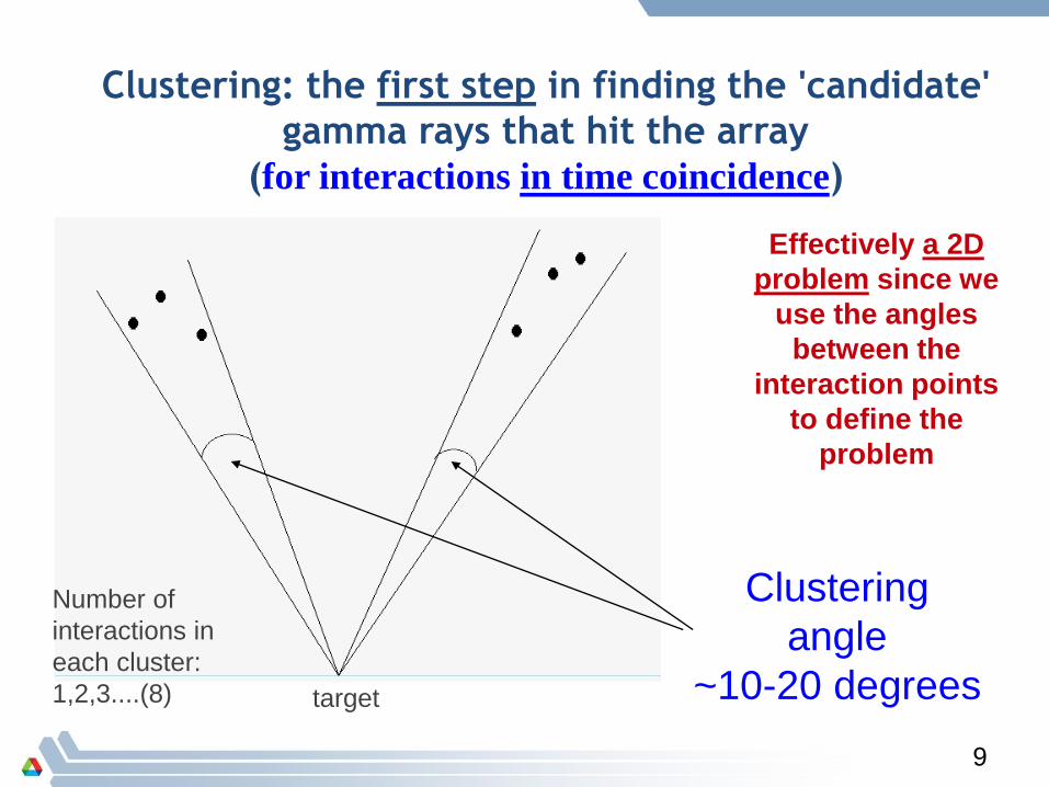
Clustering: the first step in finding the 'candidate'

gamma rays that hit the array

(for interactions in time coincidence)

Clustering

angle

~10-20 degrees

Effectively a 2D

problem since we

use the angles

between the

interaction points

to define the

problem

target

Number of

interactions in

each cluster:

1,2,3....(8)

10

Cluster angle and n, the virtual number of crystals

we have

alpha n

10 525 | Typical tracking cluster angles

15 234 |

17 180 | <- AGATA crystal, nominal dist

20 132 |

21 120 <- GRETINA crystals, nominal dist

22 108 <- Gammasphere module

(deg)

11

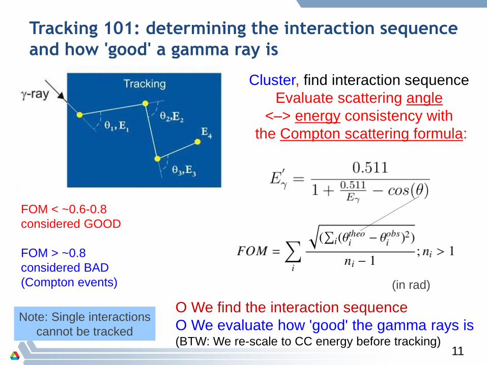
Tracking 101: determining the interaction sequence

and how 'good' a gamma ray is

Cluster, find interaction sequence

Evaluate scattering angle

<–> energy consistency with

the Compton scattering formula:

FOM < ~0.6-0.8

considered GOOD

FOM > ~0.8

considered BAD

(Compton events)

Note: Single interactions

cannot be tracked

(in rad)

O We find the interaction sequence

O We evaluate how 'good' the gamma rays is (BTW: We re-scale to CC energy before tracking)

12

FOM: a measure of how well the interaction angles and

interaction energies follow the Compton scattering formula

for the interaction points in a gamma ray. Typical spectrum

of FOM values (in log):

Single hits, FOM==0

Single interaction

over range

Over

flow‘mostly bad guys’

‘mostly good guys’

Typical FOM cut

13

Examples of good photo peak events, 3D plots

ndet= 4 esum= 0.8111/

Bestperm=00003/

FOM= 0.1333;

ndet= 4 esum= 0.7119/

Bestperm=00018/

FOM= 0.2392;

The interactions can be

spread over more than

one crystal, – the tracking

algorithm does not care

166Ho data

14

For single hits: We can improve the tracking by other means:

... it does help!

back

front

50 % absorption

Looks like a

low energy

'single

interaction'

Escape

lost

== Mean Range

''Virtual Compton shield''

15

For single hits: We can improve the tracking by other means:

Looks like a

low energy

'single

interaction'

Escape

lost

RejectSingle hits fom=0

Single interaction over range

Absorption Probability

16

Summary: Tracking and

sorting practicalities

Traces

Decomp

(PSA)

Global

Event build

Track

Sort

Digitized traces of charge collections:

from Central Contact (CC) and

segments (net and induced)

From the traces: find the (x,y,z,e,t)

data from fits to the traces

Collect and time order the

(x,y,z,e,t) data + add external data

Find coincidences, Cluster and Track.

First time we can talk about 'gamma rays'

ext

Sort the [ext],(mode3), mode2 and

mode 1 data (e.g., with GEBSort)

GT

Off-

line

mode3

mode2

mode2

mode2 + mode1

17

Universal: GT Header/Payload scheme

also used for any AUX detector systems:

Paylo

ad

header

struct gebData {

int type; /* type of data following

*/

int length;

long long timestamp;

};#define GEB_TYPE_DECOMP 1

#define GEB_TYPE_RAW 2

#define GEB_TYPE_TRACK 3

#define GEB_TYPE_BGS 4

#define GEB_TYPE_S800_RAW 5

#define GEB_TYPE_NSCLnonevent 6

#define GEB_TYPE_GT_SCALER 7

#define GEB_TYPE_GT_MOD29 8

#define GEB_TYPE_S800PHYSDATA 9

#define GEB_TYPE_NSCLNONEVTS 10

#define GEB_TYPE_G4SIM 11

#define GEB_TYPE_CHICO 12

#define GEB_TYPE_DGS 14

#define GEB_TYPE_DGSTRIG 15

#define GEB_TYPE_DFMA 16

#define GEB_TYPE_PHOSWICH 17

#define GEB_TYPE_PHOSWICHAUX 18

.

.

18

Selected Chat file options:

dtwin 30

target_x 0

target_y 0

target_z 0

CCcal CCenergy.cal

useCCEnergy

clusterangle 1 20

clusterangle 30 20

enabled "0-180"

trackingstrategy 1 0

trackingstrategy 2 0

trackingstrategy 3 0

trackingstrategy 4 0

trackingstrategy 5 0

trackingstrategy 6 5 ggtttt

trackingstrategy 7 5 gggtttt

trackingstrategy 8 5 gggttttt

recluster1 0.01 0.1 3 10 0.90

nprint 20

singlehitmaxdepth 23 1.9 18.5 1.0

0.000 0.59

.

.

.8.000 10.17

10.00 10.01

16.3 20.0

There are many more options!

Here we just show the basic ones.

We add mode1 data to

the mode 2 data!!!!

./trackMain \

track_GT.chat \

GTDATA/mode2.dat \

GTDATA/mode1.gtd >

GTDATA/trackMain.log(10 nsec units)

19

Some functions in tracking

Single interaction range (already covered)

Splitclusters: try to split clusters that have a bad FOM into two gamma rays that have good FOMs. [example later for summed lines]

Combine clusters: try to combine that have bad FOMs into one gamma rays that has a good FOM

Recluster: split gamma rays with bad FOM decreasing the clustering angle. [can go the other way too]

Matchmaker: combine two single interaction gamma rays into one gamma ray with a good FOM [tricky!]

We can execute these

functions iteratively until we

have made the best out of

the data we were given

The problem: sometimes

we make the wrong call

because the experimental

data is not perfect (i.e., we

accidentally destroy

good gamma rays)

20

Types of spectra we have:

CCsum (core common): each energy in the central contact (CC) is binned in a spectrum. Natural spectrum in Gammasphere; but 'compromised' in tracking arrays because of the scattering between the crystals. A scattering correction factor Cs must be introduced.

CCcal (or CCadd): the sum of all the energies in the CC is added up in a spectrum

This is the calorimetric spectrum. Used mostly to determine the efficiency of a tracking array. It treats the arrays as just one detector, corrections are substantial.

After tracking, we have Tracked spectra: clustered and 'evaluated spectra'. They depends on the tracking parameters, in particular, the clustering angle and the FOM cut

We would like to determine the efficiency for

these spectra. From CCsum and CCcal we

get the array photopeak efficiency.

We have two methods

CSM: Calibrated Source Method

SPM: Summed Peak Method

Both CCsum and

CCcal are

'complicated' spectra

in tracking arrays

(compared to

Gammasphere)

21

How tracking improves the spectra: 166Ho compare: CCsum

(ref), CCadd, clustered and tracked

The

simplest

thing one

can do

Calorimetric

mode, m>1 is a

disaster

(summed lines)

Offset

plots!

22

Like having 'virtual

crystals', need not align

with physical crystals

How tracking improves the spectra: 166Ho compare: CCsum

(ref), CCadd, clustered and tracked

23

The ultimate: Both clustered

and evaluated as being

'good' or 'bad' gamma rays

How tracking improves the spectra: 166Ho compare: CCsum

(ref), CCadd, clustered and tracked

24

The packing of the array matters!

Compactness: number of crystal sides that

have close neighbors to total number of

crystal sides. Best we had was 71% at MSU

~63% compactness

for ANL setup.

BTW: at MSU, typically a

more open packing is used in

order to take advantage of

the Lorenz boost. So tracking

is not always used here...

25

Efficiency of tracking arrays, *it is complicated*

Observed areas for 60Co source with

[N==1,Cs==0] for

CCadd and N

number of crystals for

CCsum where Cs>0

Correct for the fact that the

1173 can knock out counts

in the 1333 line and vice

versa. CCcal: big effect,

CCsum smaller effect

Live fraction

F: addback factor

Cfis the angular correlation

factor small correction for CCcal

bigger for CCsum

See

NIMA59201

(In print)

26

Summed Peak Method: SPM

[A(2506)/A(1173 method]

Calibrated Source Method: CSM

[S and Lfmust be known]

With CCcal and CCsum: four

measurements of the array efficiency

Also have

external/internal

detections of 1173

27

True areas and true P/T (new concepts)

Include for

CCcal and

CCsum but not

for tracked

spectra

28

Tracking efficiency and P/T for GRETINA

Analysis of data

from GRETINA

at ANL:

Compactness

was 63%. Best

setup had

compactness of

71% and yielded

a better P/TWeighted mean: 6.27(4)% for 28 crystals

(included external/internal measurements too)

29

Tracking Basics:

The usual

efficiency and P/T

compromise!

nsi: no single

interactions

wsi: with single

interactions28 crystals and

compact MSU

setup

30

92Mo case: energy resolution in

GT is much better at 2 MeV for fast moving

beams! Need tracking

to find first interaction point

GS sort using side channels (rebel)

V/C=8.8%

Double gated spectra

Background subtracted

GT uses FOM<0.8

Where GT

shines:

GT

GS

31

Matrices with and without tracking [166Ho]

Lots of Compton-Compton

coincidence that will

obscure your photo peak

coincidences

Much improved, but

not perfect Log

scale

32

The clustering 'hole':

observe it through the angular correlation

60Co source in GT

and AG

Clustering angle 10

deg

Gamma rays in the

same clustering

angle gets added up

and not split as they

should have been...

[there is a trick from

the AG group: 'split

before track']

33

GEANT4 Simulations

Lew Riley

Ursinus CollegeGEANT4 - GRETINA Simulationbitbucket.org/lriley/ucgretina

Adapted from the AGATA simulation code

UCGRETINA

Typical MSU

Configuration

(not compact)

34

P/T curves: GEANT4 and measured for 60Co

Regarding the

P/T: GEANT4

says we should

be doing better

than we are..

Simulation

needs to be

improved too

35

The radius spectrum. It should be smooth, but it

has structure

Decomposition (or electronics?)

prefers to place Interactions near

segment boundaries...

36

We have some GT and AG ‘data quality’ issues.

Attempt to display interaction points in 3D using ROOT

(preliminary analysis)

GT decomposition has

‘preferred’ interaction

regions for most crystals.

We see that clearly when

we slice through the crystals.

Not good for tracking

CAREFUL!!!!

There are

counts in

between.

Just a ROOT

display feature..(AGATA has similar problems...)

37

FOM<2.0

FOM<0.8

FOM>0.8

FOM cuts

The bad interaction

areas are associated with

'bad' FOM gamma rays

166Ho

But be careful with ROOT 3D plots....

38

The 'pesky' summed lines, examples from 166Ho

source:

Photo peak

FOM distribution

for 711 keV

711 keV

810 keV

184 keV

184+810=994 keV

summed line.

The

FOM distribution is

surprisingly nice

+

39

Example of tracks from summed line

0: (valid) ndet= 5 esum= 0.9922/bestperm=00005/FOM= 0.3248; (tracked)

# IP-> ( -17.69 7.36 1.76 ) order: 0 ; r= 19.25 cm e= 0.411/s= 0.411; 0, ts=25670256278;

# .. ( -17.91 6.79 1.56 ) order: 1 ; r= 19.22 cm e= 0.265/s= 0.676; 1, ts=25670256278;

# .. ( -18.03 6.35 0.15 ) order: 4 ; r= 19.11 cm e= 0.133/s= 0.809; 4, ts=25670256278;

# .. ( -18.30 3.92 0.44 ) order: 3 ; r= 18.72 cm e= 0.103/s= 0.912; 3, ts=25670256288;

# .. ( -19.02 4.95 0.38 ) order: 2 ; r= 19.66 cm e= 0.080/s= 0.992; 2, ts=25670256288;

182+810=992

40

AGATA and GRETINA

29 crystals positioned at 23.5 cm 28 crystals positioned at 18.5 cm

4.25% = 29/28 [(18.5/23.5)^2] * 6.4% (GANIL data, from A. Korichi)

FYI: We can handle AGATA data too.

It is instructive to compare!!

Interesting differences we can learn from...

41

Challenges and future:

We are still working on optimizing the tracking parameters using a 166Ho source

We need to improve the P/T. We have to find out where the improvement might come from: electronics, decomposition or tracking

The split-cluster tracking function has 'problems' (summed lines)

We are working on improving the combinecluster function

Move the GEANT4 simulations closer to the measured data

More comparisons GRETINA ↔ AGATA to understand our problems (AGATA-GRETINA collaboration meeting at ANL Dec 5-7)

You can download the GRETINA tracking package from

http://www.phy.anl.gov/gretina/GEBSort

Or via the main GRETINA web page:

http://gretina.lbl.gov

Questions: torben@anl.gov

42

Extra slides

43

FYI: We can handle AGATA data too!

We can translate Pulse Shape Analyzed (PSA) AGATA data to the GRETINA mode2 data

We can then send the AGATA data trough the GRETINA tracking and sorting codes

Thus, we can compare

44

166Ho source, T1/2=1200 years, not

expensive

45

166Ho source lines

46

Compare GEANT4

simulation with

measured data for

the 166Ho source

47

The Support Frame

RING ANGLE SLOTS

1 - -

2 58 4

3 90 8

4 122 5

5 148 5

30 holes

120 crystals

48

We have some GT and AG ‘data quality’ issues.

Attempt to display interaction points in 3D using ROOT

(preliminary analysis)

'Looks' more uniform:

expect better tracking,

but we don't see that

(we are working on this)

GT decomposition has

‘preferred’ interaction

regions for most crystals.

We see that clearly when

we slice through the crystal

CAREFUL!!!!

There are

counts in

between.

Just a ROOT

display feature..

NOTE:

Smoothed

data looks

different!