FEDERAL AVIATION ADMINISTRATION GAST-D Validation Report Results from the HI INR Development Contract 3/19/2013 Document includes the objectives, flight test plan, and results from the HI INR GAST-D Avionics Development contract.
Transcript
FEDERAL AVIATION ADMINISTRATION
GAST-D Validation Report Results from the HI INR Development Contract
3/19/2013
Document includes the objectives, flight test plan, and results from the HI INR GAST-D Avionics Development contract.
5. Summary & Future Work .............................................................................................................. 26
Appendix I: Final Report on The Development of Airborne Equipment Class (AEC) D Avionics
for the LAAS (Honeywell)……………………………………………………………………………………………………... 27
2
1. Introduction
1.1. Overview
In August 2010, a cost-sharing contract was awarded to Honeywell International to implement GAST-D algorithms, as described in the LAAS MOPS (DO-253C), on their commercially available GAST-C platform, the Integrated Navigation Receiver (INR). After each phase of implementation was completed, flight testing was conducted by the FAA Office of Advanced Concepts & Technology Development, Engineering Development Services Division, Navigation Branch ANG-C32. The objectives were to confirm that the various monitor thresholds set forth in the MOPS were appropriate and that all MOPS requirements are clearly and correctly defined.
1.2. Tasks and Schedule
Table 1.2-1 shows the major objectives of the contract, along with the INR version they were completed in if applicable and the delivery date.
Task INR Version Delivery Date
Task Area I
Delivery of 3 Baseline Receiver (INR) Units E100 11/2010-2/2011
Delivery of Bench Test Interface Software E100 12/2010
Delivery of CAT-I Compliance Report E100 9/2010
Task Area II Phase I
Implement CAT III Message Format (DO-246D LAAS ICD)
This report details the flight testing equipment and procedures used by ANG-C32. Results from flight testing are shared with the goal of confirming that the MOPS requirements have been correctly implemented and validated.
2. Flight Testing The data presented in this report was collected during flight tests at the Wm. J. Hughes Technical Center by the Office of Advanced Concepts & Technology Development, Engineering Development Services Division, Navigation Branch ANG-C32. A description of general flight test procedures follows.
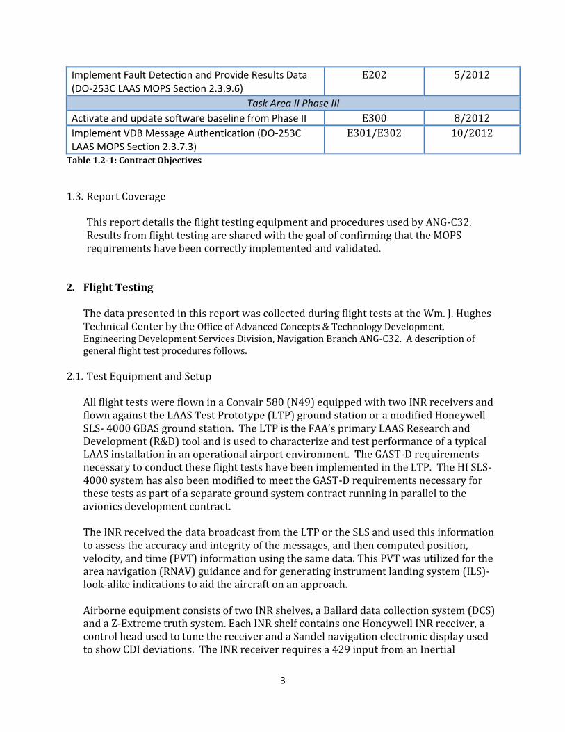
2.1. Test Equipment and Setup
All flight tests were flown in a Convair 580 (N49) equipped with two INR receivers and flown against the LAAS Test Prototype (LTP) ground station or a modified Honeywell SLS- 4000 GBAS ground station. The LTP is the FAA’s primary LAAS Research and Development (R&D) tool and is used to characterize and test performance of a typical LAAS installation in an operational airport environment. The GAST-D requirements necessary to conduct these flight tests have been implemented in the LTP. The HI SLS-4000 system has also been modified to meet the GAST-D requirements necessary for these tests as part of a separate ground system contract running in parallel to the avionics development contract. The INR received the data broadcast from the LTP or the SLS and used this information to assess the accuracy and integrity of the messages, and then computed position, velocity, and time (PVT) information using the same data. This PVT was utilized for the area navigation (RNAV) guidance and for generating instrument landing system (ILS)-look-alike indications to aid the aircraft on an approach.
Airborne equipment consists of two INR shelves, a Ballard data collection system (DCS) and a Z-Extreme truth system. Each INR shelf contains one Honeywell INR receiver, a control head used to tune the receiver and a Sandel navigation electronic display used to show CDI deviations. The INR receiver requires a 429 input from an Inertial
4
Reference System to provide the PVT output. The Convairs use a custom Honeywell HG-1095 Laser Ref IRS which used two extra bits of data resolution in place if SDI bits. This requires the Ballard DCS to take the output of the IRS, modify the 429 words and retransmit to the INR.
The Ballard DCS consists of a twelve channel 429 receive module, four channel 429 transmit module and a 4 channel rs-232/422 receive module and an ESE-291 GPS based time code generator. All 429 and RS-232 ports transmitted from the INR were collected and time stamped by the DCS and saved on a four gigabyte compact flash card. The DCS has an additional function of modifying some of the INR 429 messages and transmitting them to the Convair’s MLS port to be displayed on the ship’s CDI. This is the only way of displaying CDI information to the pilots.
The Z-Extreme is a dual frequency receiver that provides truth GPS measurements on the test aircraft and ground, independent of the GBAS equipment. A ground-based Z-extreme is used for reference and will be connected to a precision surveyed antenna. Post-processing of the data collected by this system provides accurate aircraft position over the course of a flight.
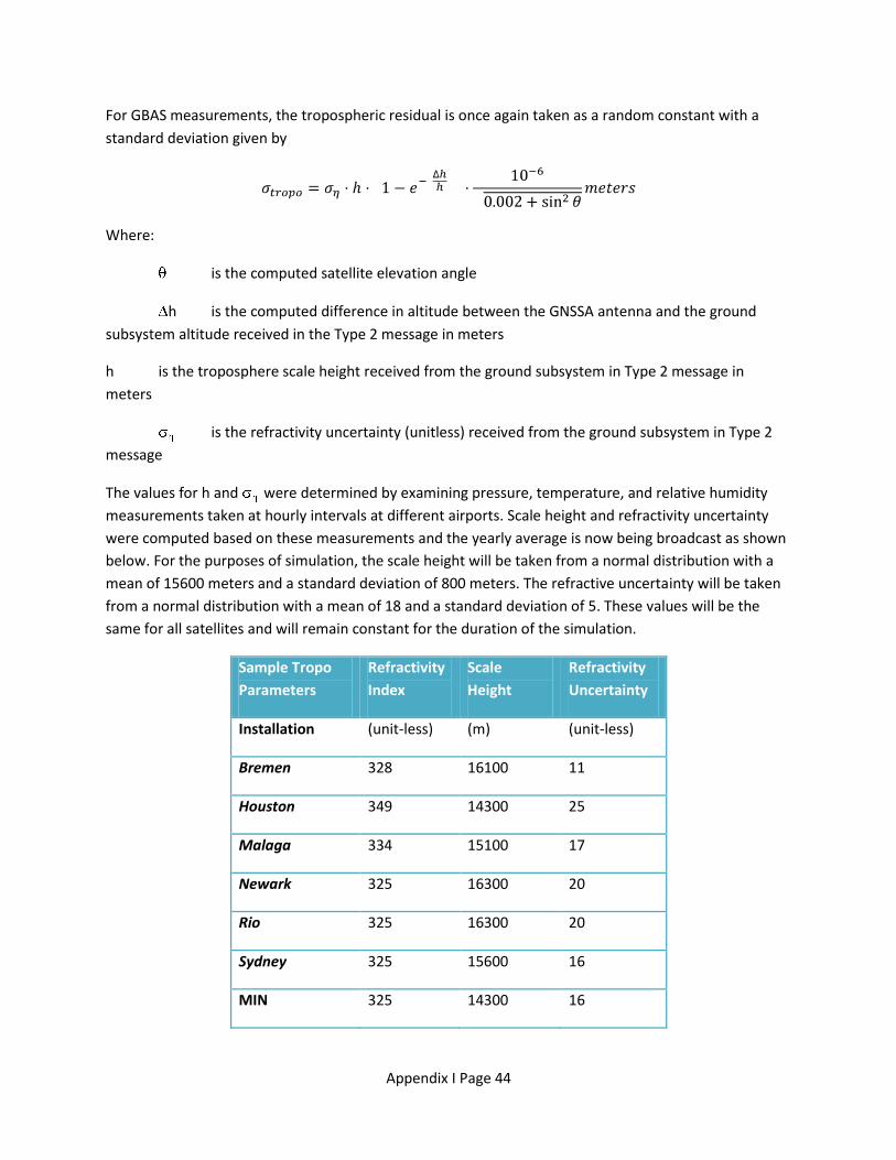
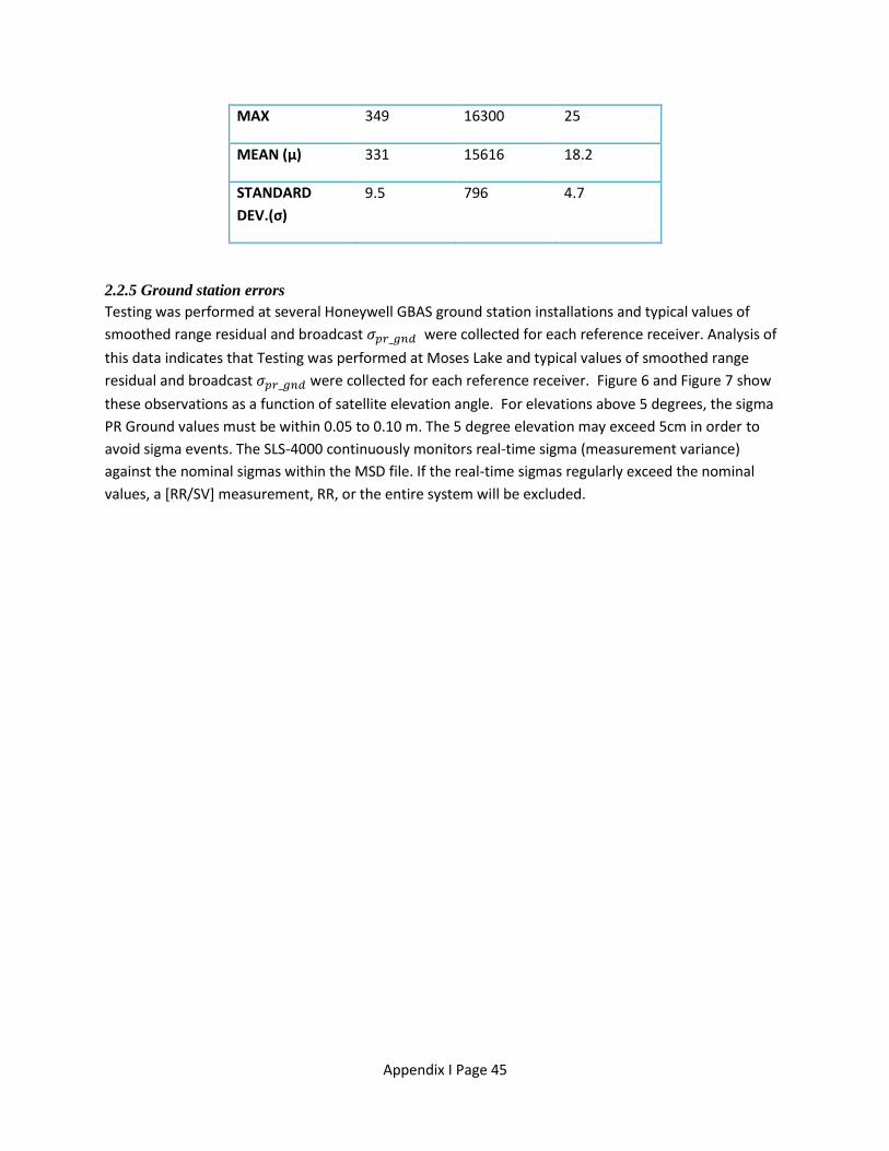
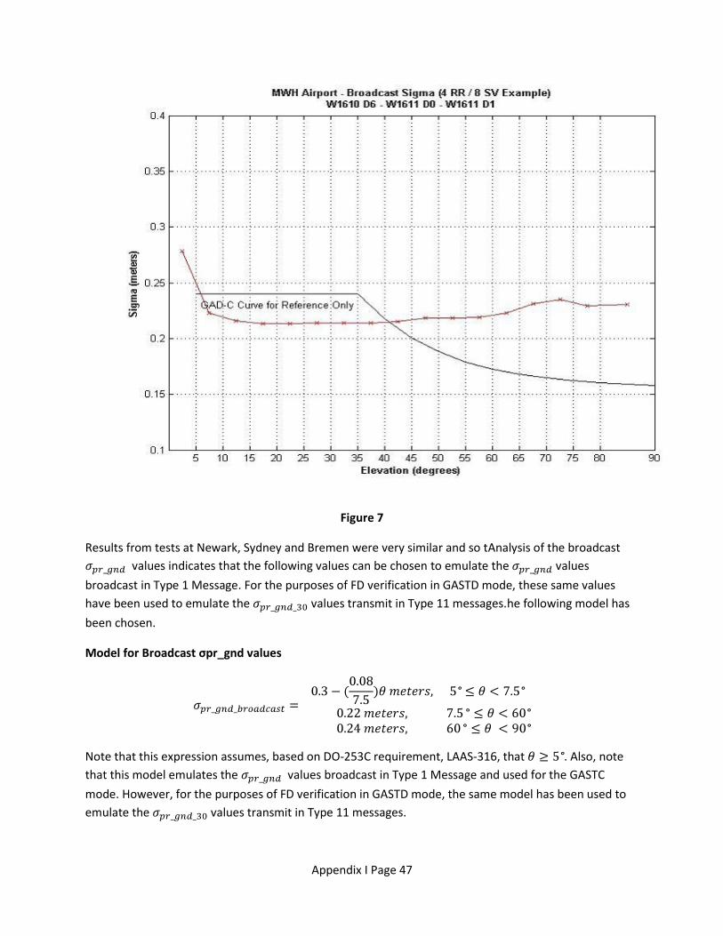
2.2. Flight Test Objectives/Profiles
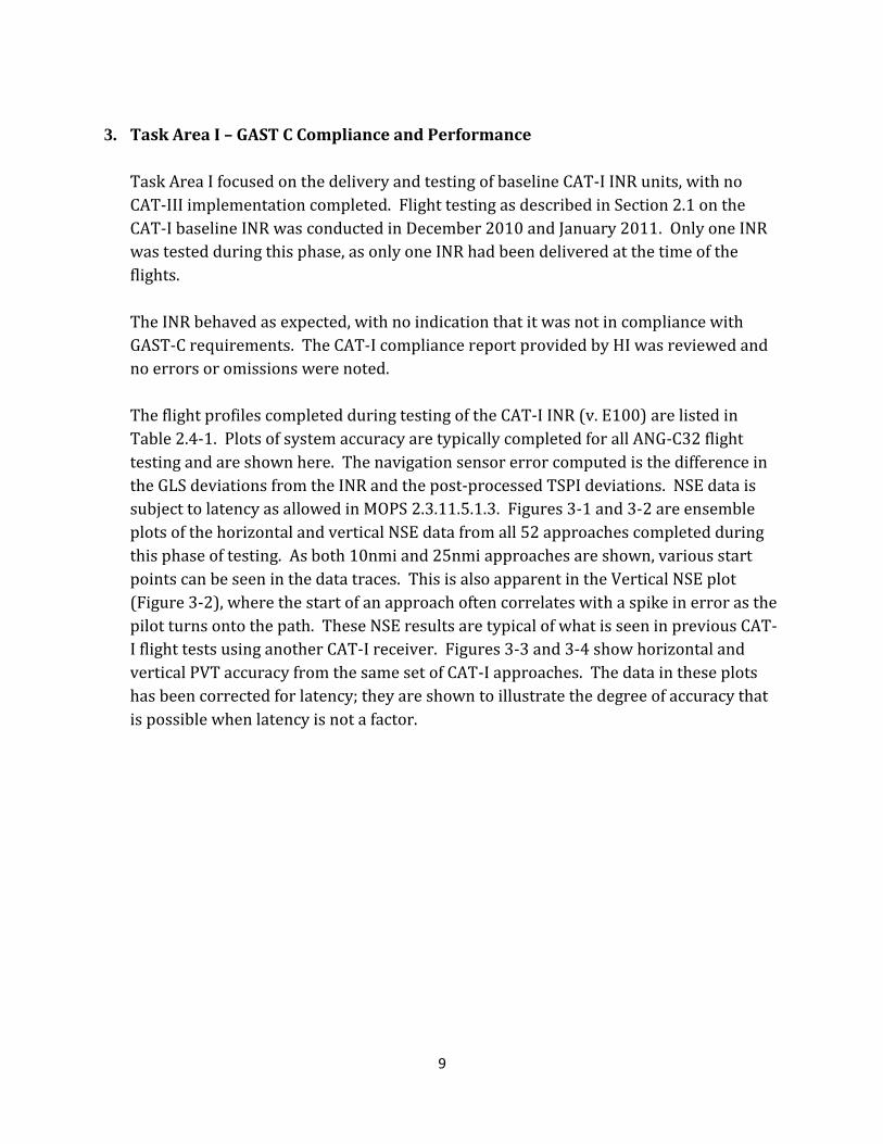
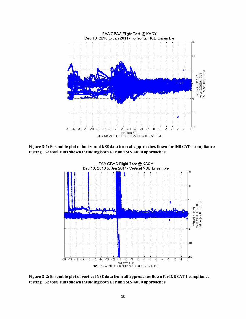
The objective of these flight tests was to evaluate the performance of the INR receiver in a fault-free environment. Six sets of flight tests were conducted during evaluation of the INR. One set of flight testing was completed after completion of Task Area I, one after Task Area II Phase 1, two during and after completion of Phase 2, and two during and after completion of Phase 3. Flight tests generally include a 20 mile orbit flown to measure VDB signal strength and verify the availability of FAS data at all four runway ends at ACY. Additionally, 20 mile radials –using runway 13-31 or runway 04-22 will be flown at approximately 3000 feet above ground level (AGL). These radials are flown to establish any VDB nulls. All approaches flown during testing will be straight-in at 3-degrees, and ILS-like. Approaches will start at either 10 or 25nmi from runway threshold. There are always several 25nmi approaches to each runway to confirm Dmax, which is set at 23.7 miles. This requires flying out of coverage and turning in to the runway approach at an altitude of 7000 feet to capture the glideslope within the Dmax range. All approaches were flown in Visual Flight Rules (VFR) and were flown either manually or coupled to the flight director, at the discretion of the pilot. Aircraft speed was approximately 170 knots.
Flight testing phases usually took place over a two week period, consisting of up to ten weekdays of available flight time. This allowed time for missed days due to weather or airplane maintenance issues if necessary. Exact numbers of approaches to each runway and of 10 or 25nmi length vary from flight test to flight test, but the following is a general guideline of the profiles flown:
5
1) Two 20nmi orbits 2) Four 20nmi radials 3) Four 25nmi approaches to RWY 31 4) Four 25nmi approaches to RWY 13 5) Four 25nmi approaches to RWY 04 6) Four 25nmi approaches to RWY 22 7) Twelve 10nmi approaches to RWY 31 8) Twelve 10nmi approaches to RWY 13 9) Twelve 10nmi approaches to RWY 04 10) Twelve 10nmi approaches to RWY 22
2.3. Additional Data Collection and Analysis for Task Area II Flight Testing
During Task Area II flight testing, additional data collection and analysis took place in order to observe data resulting from the new implementation of GAST-D algorithms. This data is made available by the modified INR.
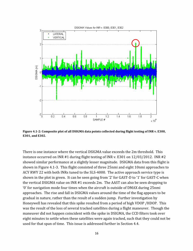
2.3.1. Task Area II Phase I Flight Testing INR data packet 0x5f, “GBASD Position Solutions”, was recorded during this phase of flight testing. This packet includes 30- and 100-second position solutions, as well as DSIGMA values DLAT and DVERT. This data was decoded and plotted. Any DSIGMA values greater than the two meter threshold indicated in the MOPS were further investigated, as were any anomalies in the position solutions.
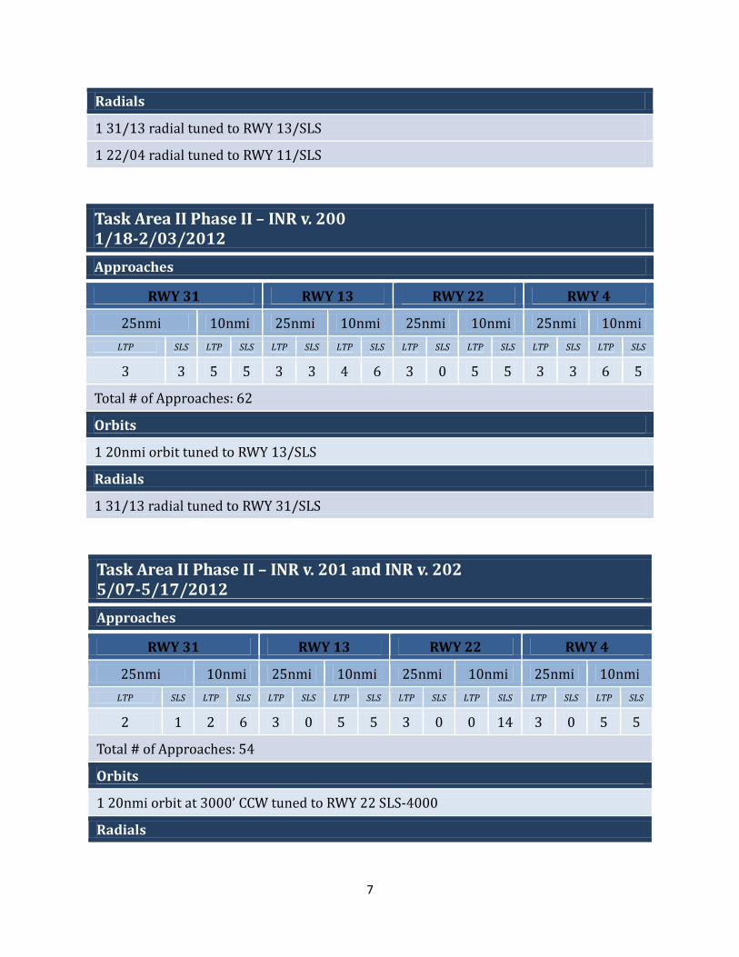
2.3.2. Task Area II Phase II Flight Testing
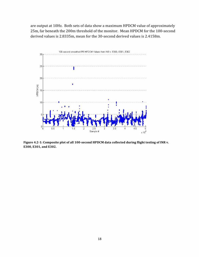
In addition to the data collected during Task Area II Phase I flight testing, data packets 0xAC “HPDCM”, 0xB9 “RRFM Parameters”, and 0xBA “FD GBAS SV Addition” were recorded. The HPDCM (Differential Correction Magnitude Check) packet provides 30- and 100-second values for the HPDCM monitor. This data was decoded and compared to the 200 meter threshold indicated in the MOPS. In this phase, values from the RRFM (Reference Receiver Fault Monitoring) and FD GBAS SV Addition (Fault Detection for SV Addition) packet were used to help determine
appropriate values for the σD_VERT and σD_LAT values needed by the RRFM algorithm. 2.3.3. Task Area II Phase III Flight Testing
For Phase III flight tests, INR data packet 0xBB “VDB Message Authentication Parameters” was decoded for analysis. This packet contains information on the slot group definition, SSIDs, and age of the Type 2 message, as well as flags for the various VDB authentication failures that can occur. The RRFM data packet, 0xB9,
was updated for this phase to include computed values for σD_VERT and σD_LAT . The
6
data packets used in analysis of the previous two phases continued to be recorded and decoded as well.
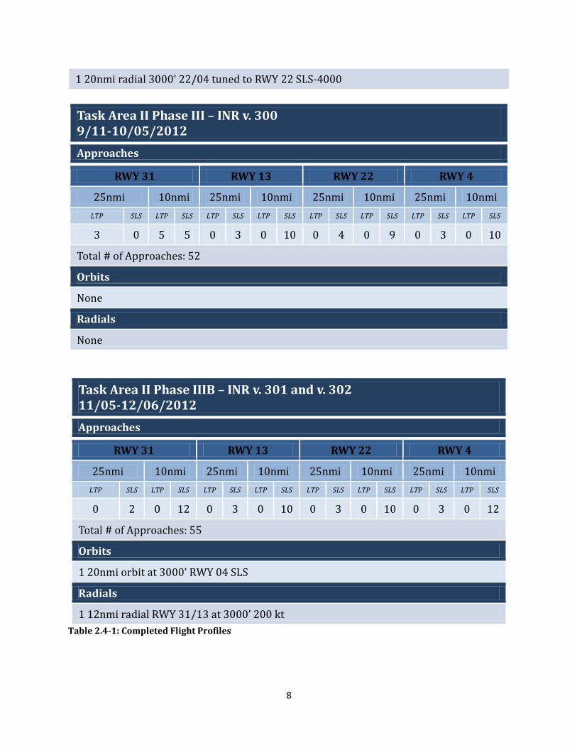
2.4. Summary of Completed Flight Profiles
Table 2.4-1 shows the details of all flight testing completed.
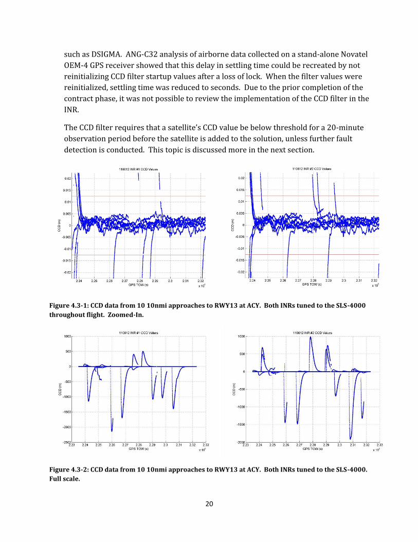
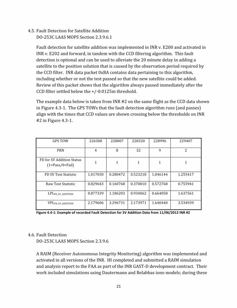
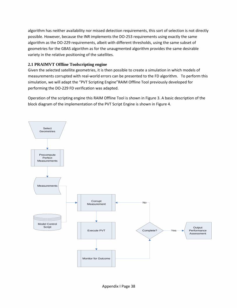
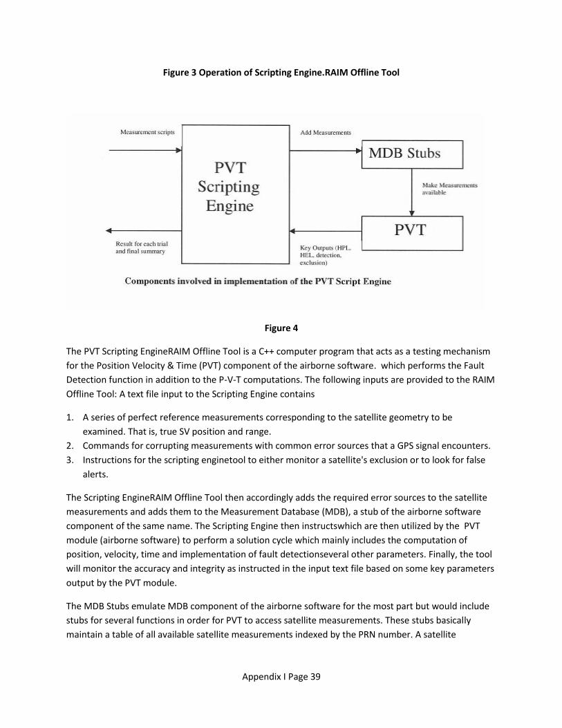
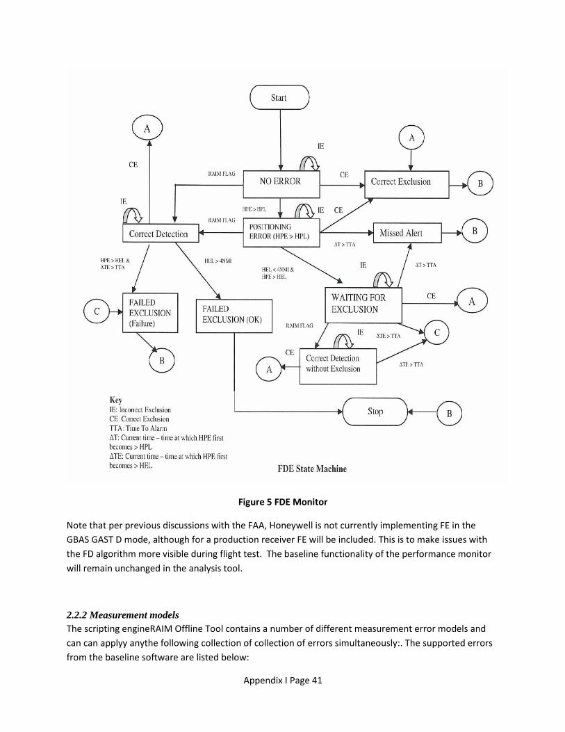
Figure 4.4-1: Example of recorded Fault Detection for SV Addition Data from 11/06/2012 INR #2
4.6. Fault Detection
DO-253C LAAS MOPS Section 2.3.9.6
A RAIM (Receiver Autonomous Integrity Monitoring) algorithm was implemented and
activated in all versions of the INR. HI completed and submitted a RAIM simulation
and analysis report to the FAA as part of the INR GAST-D development contract. Their
work included simulations using Dautermann and Belabbas iono models; during these
22
simulations no false alerts were observed. Missed detection tests were also run and no
missed alerts were observed. The details of these tests and the results can be found in
“Evaluation of GBAS Fault Detection Performance Introduction”, included as an
appendix in the HI “Final Report on the Development of AEC D Avionics for the LAAS”.
Though this fault detection is only required for GAST-D equipment, HI believes that it
would be useful for GAST-C equipment as well in detecting local causes of erroneous
measurements.
RAIM status is available in INR output data packet 0x31 “GNSS Status”. This value was
collected during all flight testing, and no RAIM alerts were observed.
4.7. Reference Receiver Fault Monitoring (RRFM)
DO-253C LAAS MOPS 2.3.11.5.2.3
Work on Reference Receiver Fault Monitoring began in INR v. E200. This version
computed and output all parameters used by the algorithm except for σD_VERT and
σD_LAT, as a decision on how to compute these values had not yet been determined. INR
v. E201 added outputs for three different possible computations of σD_VERT and σD_LAT,
respectively considering ionospheric variance only, ionospheric variance and
multipath, and ionospheric variance, multipath, and receiver noise.
Figure 4.6-1, below, shows examples of RRFM results using each of the three
calculations for σD_VERT and σD_LAT. This data was collected during flight testing of INR v.
E201 on 5/14/2012. During this flight the INRs were tuned to the SLS-4000—data is
from five 10nmi approaches to RWY 13 followed by two 10nmi approaches to RWY 22.
RRFM values are computed regardless of aircraft position in this version. Data at the
start of each plot was recorded while the airplane was on the ground. Accounting for
multipath allows the thresholds to be inflated during this time.
23
Figure 4.6-1(a): Lateral and Vertical RRFM Test Statistics and Thresholds. Computation of σD
considers iono variance only.
Figure 4.6-1(b): Lateral and Vertical RRFM Test Statistics and Thresholds. Computation of σD
considers iono variance and multipath.
Figure 4.6-1(c): Lateral and Vertical RRFM Test Statistics and Thresholds. Computation of σD
considers iono variance, multipath, and receiver noise.
RRFM was activated in v. E300 using the third means of computing for σD_VERT and
σD_LAT —considering ionospheric variance, multipath, and receiver noise. HI believes
that this implementation will provide sufficient margin to avoid false alerts on the
RRFM monitor. A failure of this monitor results in a demotion to GAST-C mode.
Periodically an upgrade to GAST-D is attempted and achieved if the monitor passes.
During flight testing of INR versions E300, E301, and E302, with RRFM activated, no
cases of the test statistic exceeding the calculated threshold were observed, either
lateral or vertical, on either of the two INRs flown. In v. E300 and on, RRFM values are
calculated only when the aircraft is within the PAR. Figure 4.6-2 shows the computed
σD values from these flight tests. The more elevated values seen throughout the plot
24
are due to the inflation of the σs for multipath when the aircraft is on the ground; each
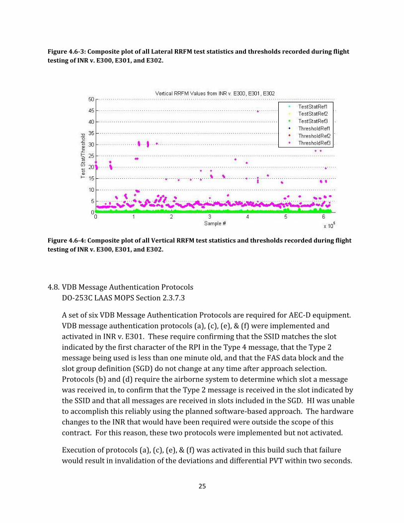
spike correlates to the data collection at the start of a flight test. Figures 4.6-3 and 4.6-
4 show composites of calculated test statistics and thresholds for lateral and vertical
RRFM tests. The data shown includes all that was collected on both INRs during flight
testing of these versions. Note that SLS RSMU #4 was unavailable. Though data for all
available references is plotted, only data for RSMU #3 is clearly seen due to the
similarity of the values for the three references. The larger magnitude data points line
up with the inflated σD values in Figure 4.6-2.
Figure 4.6-2: Composite plot of all recorded σD values from flight testing of INR v. E300, E301, and
E302.
25
Figure 4.6-3: Composite plot of all Lateral RRFM test statistics and thresholds recorded during flight
testing of INR v. E300, E301, and E302.
Figure 4.6-4: Composite plot of all Vertical RRFM test statistics and thresholds recorded during flight
testing of INR v. E300, E301, and E302.
4.8. VDB Message Authentication Protocols
DO-253C LAAS MOPS Section 2.3.7.3
A set of six VDB Message Authentication Protocols are required for AEC-D equipment.
VDB message authentication protocols (a), (c), (e), & (f) were implemented and
activated in INR v. E301. These require confirming that the SSID matches the slot
indicated by the first character of the RPI in the Type 4 message, that the Type 2
message being used is less than one minute old, and that the FAS data block and the
slot group definition (SGD) do not change at any time after approach selection.
Protocols (b) and (d) require the airborne system to determine which slot a message
was received in, to confirm that the Type 2 message is received in the slot indicated by
the SSID and that all messages are received in slots included in the SGD. HI was unable
to accomplish this reliably using the planned software-based approach. The hardware
changes to the INR that would have been required were outside the scope of this
contract. For this reason, these two protocols were implemented but not activated.
Execution of protocols (a), (c), (e), & (f) was activated in this build such that failure
would result in invalidation of the deviations and differential PVT within two seconds.
26
In v. E301, these become valid again as soon as the failure condition is cleared. The
matter of when these faults should be cleared is not currently covered by DO-253C.
Discussion at RTCA concluded that VDB failure conditions should only be cleared upon
retune.
VDB authentication data was output in INR data packet 0xBB for analysis. Type 2 data
age rarely exceeded two seconds (Type 2 data is sent every two seconds from the SLS-
4000) and RPIs were as expected. No attempt to cause these protocols to fail was
made. Further validation of protocols (b) and (d) may be necessary in the future since
their reliable implementation and activation was not possible within the confines of
this contract.
5. Summary & Future Work
The INR GAST-D development contract sought to implement GAST-D algorithms on the
HI INR. With the exception of two of the six new VDB authentication protocols, these
implementations were successfully completed. HI believes that these two protocols
would be feasible with hardware changes to the INR. The data collected during flight
testing indicates that the monitor thresholds currently specified in the LAAS MOPS DO-
253C do not cause excessive false alerts leading to loss of service during nominal
conditions. Several concerns about the clarity of some MOPS requirements were raised
during implementation and were brought to RTCA for discussion and resolution.
Details of these issues are available in HI’s “Final Report on the Development of AEC D
Avionics for the LAAS”.
There is a possibility for future work to be conducted with the INR if funding becomes
available. This work would focus on improving the airborne receiver’s robustness to
RFI. In addition, tasks such as attempting to induce failures on the new monitors,
reviewing the INR implementation of the CCD filter, implementation of the satellite
geometry screening described in DO-253C section 2.3.94, and completion of VDB
authentication protocol implementation may be considered.
FINAL REPORT
ON
THE DEVELOPMENT OF AIRBORNE EQUIPMENT CLASS (AEC) D AVIONICS FOR
THE LOCAL AREA AUGMENTATION SYSTEM (LAAS)
(Contract # DTFACT-10-D-00016)
SUBMITTED TO
FAA WILLIAM J. HUGHES TECHNICAL CENTER
Service ACQUISITION Group, AJA-47A
ATLANTIC CITY INTERNATIONAL AIRPORT, NJ 08405
January 2013
Honeywell Aerospace
One Technology Center
23500 West 105th
Street
Olathe, KS 66061
Appendix I Page 1
Contents 1. Introduction and Executive Summary 2
2. Updates to the previously certified INR 5
3. Deficiencies in the RTCA/DO-253C 15
4. Lab Tests 17
5. Flight Tests 19
Appendix A: Evaluation of GBAS fault detection performance 37
Appendix B: Ionospheric Model for GBAS Test Data Generation 53
Appendix C: Creating exponentially distributed samples from random numbers that are uniformly
distributed 56
List of Acronyms 58
1. Introduction and Executive Summary 3
2. Updates to INR 6
3. Deficiencies in the DO-253C 16
4. Lab Tests 18
5. Flight Tests 21
Plots from Final Build Delivered (E302): 22
Appendix A: Evaluation of GBAS fault detection performance 29
Appendix B: Ionospheric Model for GBAS Test Data Generation 56
Appendix C – Creating exponentially distributed samples from random numbers that are uniformly
distributed 59
List of Acronyms 61
Appendix I Page 2
1. Introduction and Executive Summary
This report summarizes the work performed under FAA contract (DTFACT-10-D-00016), dated August
18, 2010, to Honeywell Aerospace. Under the auspices of the contract, Honeywell collaborated with
the FAA towards the development of an Airborne Equipment Class (AEC) D avionics prototype. The
objectives of this program were (1) to provide the FAA Engineering Development Services Navigation
Team (ANG-C32) and the SATNAV program office with red label (non-certified) equipment, (2) to
implement and test specified messages and algorithms as described in RTCA DO-246D and DO-253C
documents and finally (3) to provide support to the Navigation Team during flight test, TERPS testing,
procedure development, LAAS Ground Facility testing, flight inspection requirements, and to validate
GBAS Approach Service Type (GAST) D requirements.
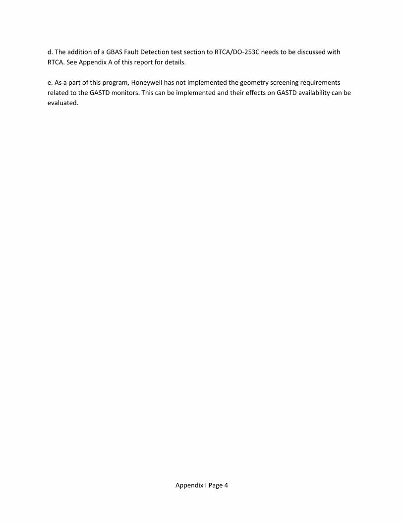
The commercial platform used as a baseline for the AEC D prototype
is the Integrated Navigation Receiver (INR). It was developed as a
platform for future navigation applications and a basis for higher
levels of aircraft system integration. The INR integrates a VHF
Omni-directional Receiver (VOR), a Marker Beacon receiver, an
Instrument Landing System (ILS) (Localizer & Glide Slope) receiver,
Dual Monitored Level-A GPS receivers, and a VHF Data Broadcast
(VDB) Receiver for DGPS. The INR is a Multi-Mode Receiver +
(MMR+) as it includes all of the typical MMR functions and adds
both VOR and Marker Beacon receiver. A picture of the hardware is
shown in Figure 1-1.
Honeywell completed the AEC C (CAT I) compliance testing for the INR
and has documented the results as part of the INR certification. Honeywell received TSO approval for
the INR on May 6, 2010. The INR was part of the avionics used in completing the first 787 GLS autoland
flight test on 2/1/2010. These test reports were provided to FAA at the beginning of the program to
demonstrate compatibility of the INR platform to validate AEC D (CAT III) requirements.
As part of the program, three baseline INR units along with a bench test interface and documentation
(developed at the beginning of the program) were delivered to FAA to provide a capability to upload
incremental software builds at the FAA facility. This enabled smooth collaboration on the program with
Honeywell incrementally implementing CAT III algorithms and FAA conducting flight tests.
Honeywell developed a series of incremental software builds in compliance with the VDB message
specifications in DO-246D and GAST D algorithms in DO-253C. Mercury3 CP GNSS is a single circuit card
assembly that is integrated with the INR. The GNSS determines position, velocity, time, integrity and
status information from GPS signals receiver via an external antenna. In addition, the GNSS further
monitor signals from the Ground Based Augmentation Systems (GBAS) in order to provide flight path
deviation data as well as to enhance system safety and accuracy. The sensor outputs this data using
serial data and ARINC 429 data lines. The GNSS is incorporated into the INR. The INR provides the
Figure 1-1: INR
Appendix I Page 3
required power to the GNSS and uses the GNSS outputs for positioning. The GNSS also uses serial or
ARINC 429 inputs to acquire initial position estimates or optional altitude aiding information. The GNSS
also supports the INR’s predictive RAIM requirements. Only the AEC C baseline software that executes in
the Mercury3 CP GNSS module, a part of the MMR (INR) hardware unit, was modified. Honeywell
verified that various monitor thresholds set forth in DO-253C were appropriate and that most
requirements were clearly defined and were correct. Some additional guidance was needed in the
document for some of the monitors and some requirements were not completely correct. Due to these
deficiencies, Honeywell had to deviate from the MOPS on some requirements. Each deviation was
discussed with the FAA before implementation and details are provided in this report. These short
comings have been presented to RTCA’s SC-159 for further evaluation.
Each software build, including both new and modified AEC C software, was tested in Honeywell’s labs
using developmental hardware. The tested software code was delivered in an object form suitable for
loading into the INR using the bench test interface. Along with each build, an updated Interface Control
Document, describing the output message formats, and MercHost Tool to record the RS-232 data output
by the INR was delivered.
Flight tests were performed by the FAA with each software update. Data from each flight test was
analyzed to observe GAST D performance.
In the following sections, this report summarizes the tasks performed to create AEC D prototype
software, deviations taken from DO-253C while implementing the algorithms for GAST D monitors,
deficiencies found in DO-253C, lab testing performed by Honeywell and flight tests performed by the
FAA.
1.1 Recommendations for Future Activities A few tasks were identified during this program but could not be completed due to timing and funding
constraints. These tasks have been listed below as recommendations for future activities.
a. The flight tests covered ideal case conditions. Trigger Conditions to induce failures of monitors like
RRFM, VDB authentication protocols, etc. that apply to GAST D, need to be created during flight tests.
b. DO-253C requires implementation of airborne CCD filter that needs to settle before measurements
can be included in GBAS mode. CCD filter output takes several minutes to settle. This prevents use of
satellites in GAST D mode and contributed to a DSIGMA failure on a flight test on December 03, 2012.
Details on this failure are provided in section 5 of this report. A study can needs to be performed to
observe the impact of initialization values on the CCD filter or enhancing the filter to accelerate shorten
the settling period.
c. VDB Authentication Protocols ‘b’ and ‘d’ were not completely implemented in this program as they
required a hardware modification to the INR which was not performed. They will need to be
implemented in the production unit and further testing of these protocols needs to be performed then.
Appendix I Page 4
d. The addition of a GBAS Fault Detection test section to RTCA/DO-253C needs to be discussed with
RTCA. See Appendix A of this report for details.
e. As a part of this program, Honeywell has not implemented the geometry screening requirements
related to the GASTD monitors. This can be implemented and their effects on GASTD availability can be
evaluated.
Appendix I Page 5
2. Updates to the previously certified INR During this project the baseline AEC C INR, previously certified to comply with TSO-C161 and DO-253A
for GAST C operation, was modified to support GAST D operations. In addition, a laboratory test
environment (a “Bench Test Interface”) was created to support the evaluation of the new and modified
functionality.
Bench Test Interface The bench test interface was developed and tested to support software loading of the GNSS
module without removing the module from the LRU at the FAA laboratory facilities. This test
set-up involved the use of the INR break-out box (p/n: 071-00265-0000) in conjunction with the
Ballard Technology’s Avionics Data Bus Model UA 1420. The INR’s break-out box provides
interfaces to all data from the INR. It is connected to the INR by a cable harness. There are
several pins provided on the break-out box that are intended to control the INR’s discrete inputs,
allow access to fault logs and to be used in loading software in the GNSS module.
The PC tool, ‘MercHost’, is used to view data from the INR RS-232 ports and to record and
examine in real-time various GPS parameters that can facilitate testing and debugging the
functions of the GNSS. MercHost was updated to support new AEC D/GAST D messages
transmitted by the INR. Ballard Technology’s Co-Pilot 5.20 was used for viewing/changing
ARINC 429 data transmitted and received via the UA 1420.
The MercHost and Co-Pilot software, the assembled and tested bench test interface along with an
INR containing the AEC C baseline software were delivered early in the project. Supporting
documentation such as the interface control document, the INR installation manual, and a
description of AEC C/GACT C compliance testing were also delivered. Figure 2-1 below gives
an overview of the test set-up.
Appendix I Page 6
Figure 2-1: Overview of the Test Set Up
AEC D Software updates The AEC C software was modified to implement the following requirements. Some requirements were
partially implemented and certain deviations were taken for a few requirements. More details on the
implementation are provided later in this section.
AEC D Requirement [DO-253C] Function Summary Honeywell Compliance
LAAS-179 LPL, VPL Full
LAAS-277 MT2, Additional Blocks Full
LAAS-287 LPB, VPB Full
LAAS-319 30s smoothing Full
LAAS-320 30s smoothing Full
LAAS-321 30s smoothing Full
LAAS-324 Airborne CCD filtering Full
LAAS-325 Airborne CCD filtering Deviation
LAAS-326 Msg Type 11 Processing Full
LAAS-327 VDB Authentication Deviation, Partial
Ballard Technology
DataBus UA 1420 RX0
RX1
TX12
TX13
RX2
RX3
INR Break out Box
ILS Look Alike 1
GNSS Data 1
IRS I/p 1, 2 and 3
Tune Function Select A &B I/p
IRS O/p 1, 2 and 3 [Echo]
Tune Function Select A &B O/p
[Echo]
RS-232 O/p
RS-232 I/p
USB
RX
PC Workstation TX
TMCP1/TMCP2
TMCP1 / TMCP2 /
PIO2
INTEGRATED
NAVIGATION RECEIVER
(INR)
Appendix I Page 7
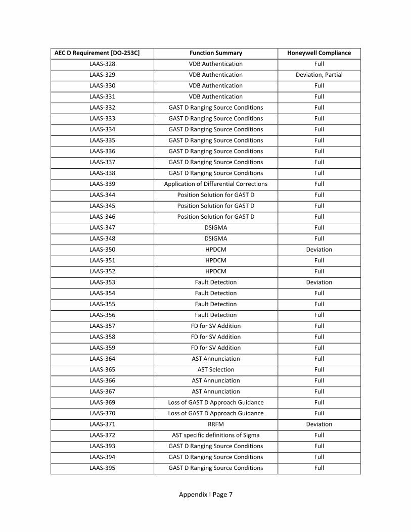
AEC D Requirement [DO-253C] Function Summary Honeywell Compliance
LAAS-328 VDB Authentication Full
LAAS-329 VDB Authentication Deviation, Partial
LAAS-330 VDB Authentication Full
LAAS-331 VDB Authentication Full
LAAS-332 GAST D Ranging Source Conditions Full
LAAS-333 GAST D Ranging Source Conditions Full
LAAS-334 GAST D Ranging Source Conditions Full
LAAS-335 GAST D Ranging Source Conditions Full
LAAS-336 GAST D Ranging Source Conditions Full
LAAS-337 GAST D Ranging Source Conditions Full
LAAS-338 GAST D Ranging Source Conditions Full
LAAS-339 Application of Differential Corrections Full
LAAS-344 Position Solution for GAST D Full
LAAS-345 Position Solution for GAST D Full
LAAS-346 Position Solution for GAST D Full
LAAS-347 DSIGMA Full
LAAS-348 DSIGMA Full
LAAS-350 HPDCM Deviation
LAAS-351 HPDCM Full
LAAS-352 HPDCM Full
LAAS-353 Fault Detection Deviation
LAAS-354 Fault Detection Full
LAAS-355 Fault Detection Full
LAAS-356 Fault Detection Full
LAAS-357 FD for SV Addition Full
LAAS-358 FD for SV Addition Full
LAAS-359 FD for SV Addition Full
LAAS-364 AST Annunciation Full
LAAS-365 AST Selection Full
LAAS-366 AST Annunciation Full
LAAS-367 AST Annunciation Full
LAAS-369 Loss of GAST D Approach Guidance Full
LAAS-370 Loss of GAST D Approach Guidance Full
LAAS-371 RRFM Deviation
LAAS-372 AST specific definitions of Sigma Full
LAAS-393 GAST D Ranging Source Conditions Full
LAAS-394 GAST D Ranging Source Conditions Full
LAAS-395 GAST D Ranging Source Conditions Full
Appendix I Page 8
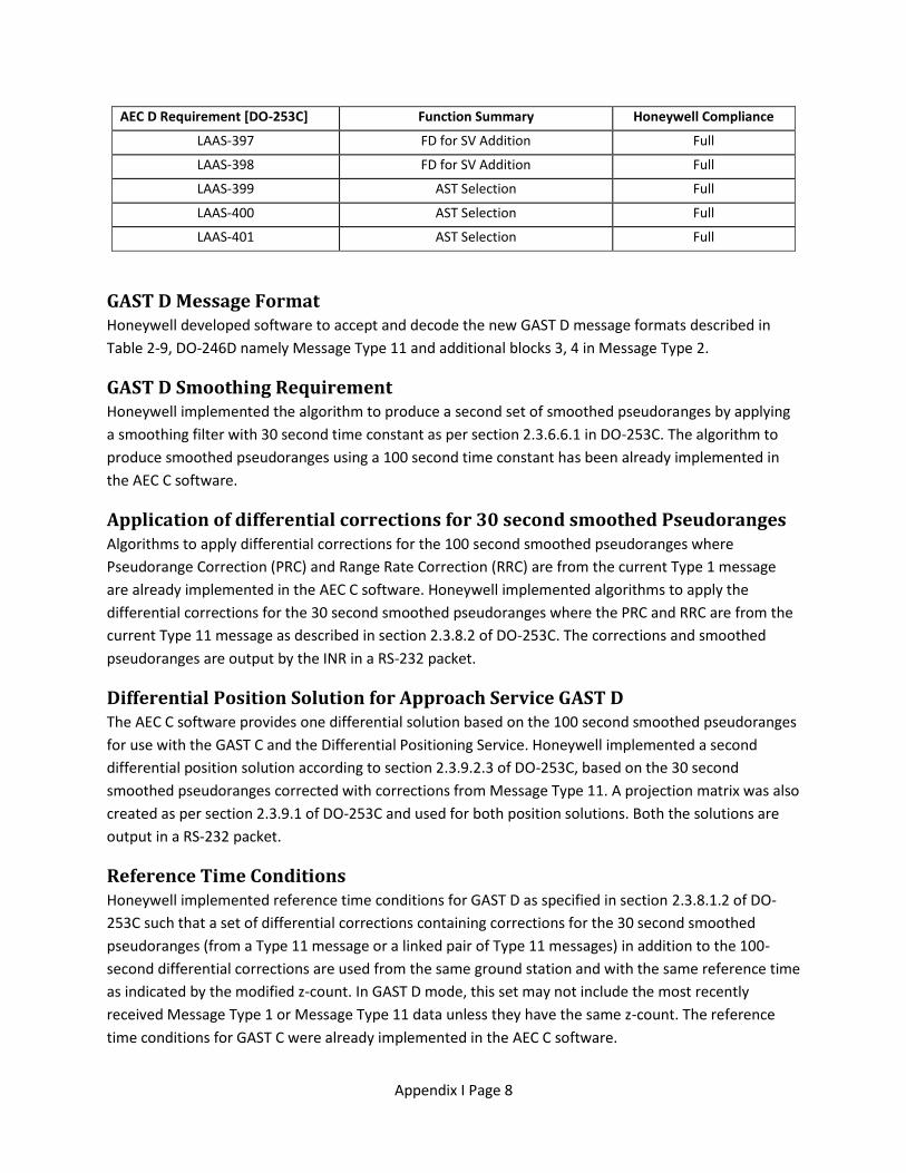
AEC D Requirement [DO-253C] Function Summary Honeywell Compliance
LAAS-397 FD for SV Addition Full
LAAS-398 FD for SV Addition Full
LAAS-399 AST Selection Full
LAAS-400 AST Selection Full
LAAS-401 AST Selection Full
GAST D Message Format Honeywell developed software to accept and decode the new GAST D message formats described in
Table 2-9, DO-246D namely Message Type 11 and additional blocks 3, 4 in Message Type 2.
GAST D Smoothing Requirement Honeywell implemented the algorithm to produce a second set of smoothed pseudoranges by applying
a smoothing filter with 30 second time constant as per section 2.3.6.6.1 in DO-253C. The algorithm to
produce smoothed pseudoranges using a 100 second time constant has been already implemented in
the AEC C software.
Application of differential corrections for 30 second smoothed Pseudoranges Algorithms to apply differential corrections for the 100 second smoothed pseudoranges where
Pseudorange Correction (PRC) and Range Rate Correction (RRC) are from the current Type 1 message
are already implemented in the AEC C software. Honeywell implemented algorithms to apply the
differential corrections for the 30 second smoothed pseudoranges where the PRC and RRC are from the
current Type 11 message as described in section 2.3.8.2 of DO-253C. The corrections and smoothed
pseudoranges are output by the INR in a RS-232 packet.
Differential Position Solution for Approach Service GAST D The AEC C software provides one differential solution based on the 100 second smoothed pseudoranges
for use with the GAST C and the Differential Positioning Service. Honeywell implemented a second
differential position solution according to section 2.3.9.2.3 of DO-253C, based on the 30 second
smoothed pseudoranges corrected with corrections from Message Type 11. A projection matrix was also
created as per section 2.3.9.1 of DO-253C and used for both position solutions. Both the solutions are
output in a RS-232 packet.
Reference Time Conditions Honeywell implemented reference time conditions for GAST D as specified in section 2.3.8.1.2 of DO-
253C such that a set of differential corrections containing corrections for the 30 second smoothed
pseudoranges (from a Type 11 message or a linked pair of Type 11 messages) in addition to the 100-
second differential corrections are used from the same ground station and with the same reference time
as indicated by the modified z-count. In GAST D mode, this set may not include the most recently
received Message Type 1 or Message Type 11 data unless they have the same z-count. The reference
time conditions for GAST C were already implemented in the AEC C software.
Appendix I Page 9
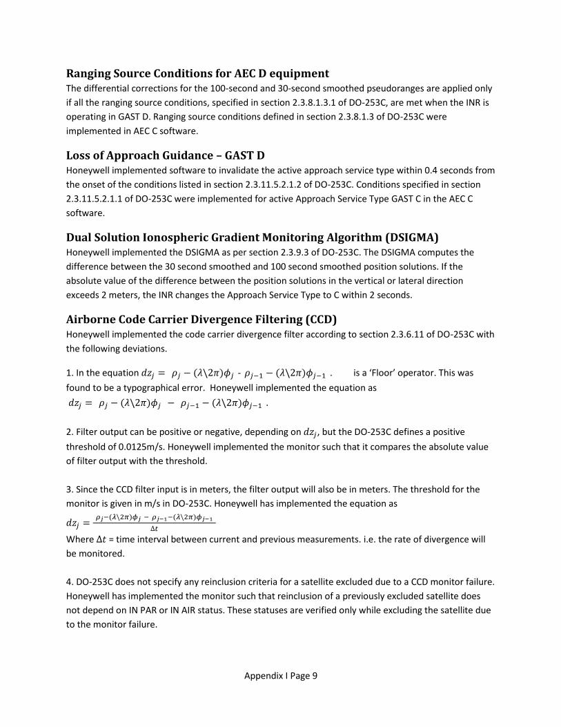
Ranging Source Conditions for AEC D equipment The differential corrections for the 100-second and 30-second smoothed pseudoranges are applied only
if all the ranging source conditions, specified in section 2.3.8.1.3.1 of DO-253C, are met when the INR is
operating in GAST D. Ranging source conditions defined in section 2.3.8.1.3 of DO-253C were
implemented in AEC C software.
Loss of Approach Guidance – GAST D Honeywell implemented software to invalidate the active approach service type within 0.4 seconds from
the onset of the conditions listed in section 2.3.11.5.2.1.2 of DO-253C. Conditions specified in section
2.3.11.5.2.1.1 of DO-253C were implemented for active Approach Service Type GAST C in the AEC C
software.
Dual Solution Ionospheric Gradient Monitoring Algorithm (DSIGMA) Honeywell implemented the DSIGMA as per section 2.3.9.3 of DO-253C. The DSIGMA computes the
difference between the 30 second smoothed and 100 second smoothed position solutions. If the
absolute value of the difference between the position solutions in the vertical or lateral direction
exceeds 2 meters, the INR changes the Approach Service Type to C within 2 seconds.
Airborne Code Carrier Divergence Filtering (CCD) Honeywell implemented the code carrier divergence filter according to section 2.3.6.11 of DO-253C with
the following deviations.
1. In the equation - . is a ‘Floor’ operator. This was
found to be a typographical error. Honeywell implemented the equation as
2. Filter output can be positive or negative, depending on , but the DO-253C defines a positive
threshold of 0.0125m/s. Honeywell implemented the monitor such that it compares the absolute value
of filter output with the threshold.
3. Since the CCD filter input is in meters, the filter output will also be in meters. The threshold for the
monitor is given in m/s in DO-253C. Honeywell has implemented the equation as
Where = time interval between current and previous measurements. i.e. the rate of divergence will
be monitored.
4. DO-253C does not specify any reinclusion criteria for a satellite excluded due to a CCD monitor failure.
Honeywell has implemented the monitor such that reinclusion of a previously excluded satellite does
not depend on IN PAR or IN AIR status. These statuses are verified only while excluding the satellite due
to the monitor failure.
Appendix I Page 10
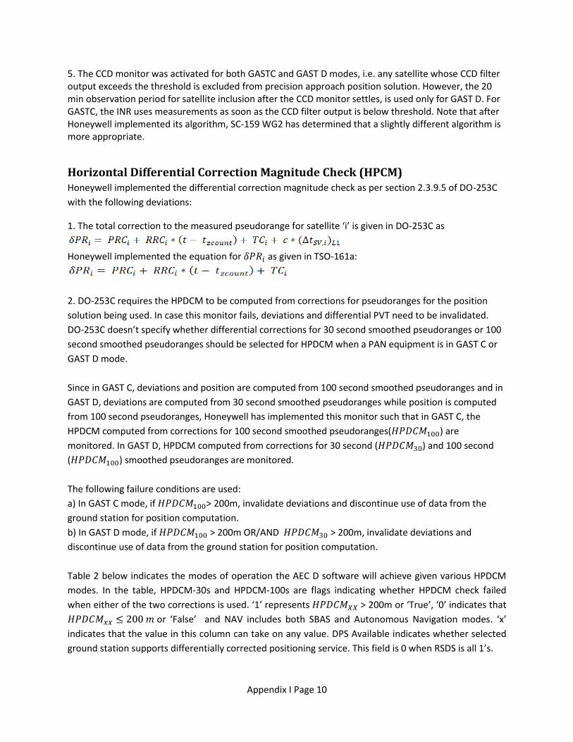
5. The CCD monitor was activated for both GASTC and GAST D modes, i.e. any satellite whose CCD filter output exceeds the threshold is excluded from precision approach position solution. However, the 20 min observation period for satellite inclusion after the CCD monitor settles, is used only for GAST D. For GASTC, the INR uses measurements as soon as the CCD filter output is below threshold. Note that after Honeywell implemented its algorithm, SC-159 WG2 has determined that a slightly different algorithm is more appropriate.
Horizontal Differential Correction Magnitude Check (HPCM) Honeywell implemented the differential correction magnitude check as per section 2.3.9.5 of DO-253C
with the following deviations:
1. The total correction to the measured pseudorange for satellite ‘i’ is given in DO-253C as
Honeywell implemented the equation for as given in TSO-161a:
2. DO-253C requires the HPDCM to be computed from corrections for pseudoranges for the position
solution being used. In case this monitor fails, deviations and differential PVT need to be invalidated.
DO-253C doesn’t specify whether differential corrections for 30 second smoothed pseudoranges or 100
second smoothed pseudoranges should be selected for HPDCM when a PAN equipment is in GAST C or
GAST D mode.
Since in GAST C, deviations and position are computed from 100 second smoothed pseudoranges and in
GAST D, deviations are computed from 30 second smoothed pseudoranges while position is computed
from 100 second pseudoranges, Honeywell has implemented this monitor such that in GAST C, the
HPDCM computed from corrections for 100 second smoothed pseudoranges( ) are
monitored. In GAST D, HPDCM computed from corrections for 30 second ( ) and 100 second
( ) smoothed pseudoranges are monitored.
The following failure conditions are used: a) In GAST C mode, if > 200m, invalidate deviations and discontinue use of data from the
ground station for position computation.
b) In GAST D mode, if > 200m OR/AND > 200m, invalidate deviations and
discontinue use of data from the ground station for position computation.
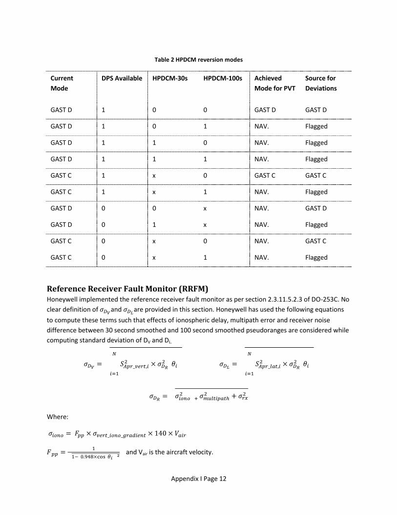
Table 2 below indicates the modes of operation the AEC D software will achieve given various HPDCM
modes. In the table, HPDCM-30s and HPDCM-100s are flags indicating whether HPDCM check failed
when either of the two corrections is used. ‘1’ represents > 200m or ‘True’, ‘0’ indicates that
or ‘False’ and NAV includes both SBAS and Autonomous Navigation modes. ‘x’
indicates that the value in this column can take on any value. DPS Available indicates whether selected
ground station supports differentially corrected positioning service. This field is 0 when RSDS is all 1’s.
Appendix I Page 11
Appendix I Page 12
Table 2 HPDCM reversion modes
Current
Mode
DPS Available HPDCM-30s HPDCM-100s Achieved
Mode for PVT
Source for
Deviations
GAST D 1 0 0 GAST D GAST D
GAST D 1 0 1 NAV. Flagged
GAST D 1 1 0 NAV. Flagged
GAST D 1 1 1 NAV. Flagged
GAST C 1 x 0 GAST C GAST C
GAST C 1 x 1 NAV. Flagged
GAST D 0 0 x NAV. GAST D
GAST D 0 1 x NAV. Flagged
GAST C 0 x 0 NAV. GAST C
GAST C 0 x 1 NAV. Flagged
Reference Receiver Fault Monitor (RRFM) Honeywell implemented the reference receiver fault monitor as per section 2.3.11.5.2.3 of DO-253C. No
clear definition of and are provided in this section. Honeywell has used the following equations
to compute these terms such that effects of ionospheric delay, multipath error and receiver noise
difference between 30 second smoothed and 100 second smoothed pseudoranges are considered while
computing standard deviation of DV and DL.
Where:
and Vair is the aircraft velocity.
Appendix I Page 13
is the airborne receiver’s multipath error when on the ground.
is the airborne receiver’s multipath error in air.
is the elevation angle.
Variance of receiver noise difference between 30 second smoothed and 100 second smoothed
pseudoranges is given as:
is the receiver noise for 30 second smoothed pseudorange.
is the receiver noise for 100 second smoothed pseudorange.
RAIM algorithm, analysis and test report Honeywell determined appropriate Receiver Autonomous Integrity Monitor (RAIM) for differential and
non-differential modes based on the analyzed performance of the Mercury3 CP GNSS receiver hardware
in the INR. A test report containing results of the analysis, describing position and range domain results
is attached in Appendix A.
Fault Detection Honeywell implemented the fault detection (FD) algorithm based in compliance with section 2.3.9.6 of
DO-253C. The FD algorithm is required to have a provide a probability of false alert less than or equal to
per sample but there is no requirement for probability of missed detection.
While DO-253C requires the FD algorithm to be executed only in GAST D mode, Honeywell believes that
the FD algorithm will be useful in detecting local conditions (like multipath) that may lead to faulted
measurements and chose to execute it in GAST C mode as well. In GAST D mode, FD is performed on the
solution that is computed using the 30 second smoothed measurements which have been differentially
corrected using data from Message Type 11. If a fault is detected in GAST D mode, the mode of
operation and thus the Approach Service Type are changed to GAST C. In GAST C mode, FD is performed
on the solution computed using 100 second smoothed measurements that have been differentially
corrected using data from Message Type 1. If a fault is detected in GAST C mode, the INR continues to
operate in GAST C mode but provides the FD annunciation.
Appendix I Page 14
Comprehensive verification of the FD algorithm was performed through a combination flight tests,
simulations and offline testing. The Offline test effort has been discussed in detail in Appendix A of this
document.
Fault Detection for Satellite Addition Section 2.3.9.6.1 of DO-253C states that if CCD filter output for a satellite is below the threshold, then it
can be immediately included in the GAST C or GAST D solution if the FD for Satellite Addition criteria are
satisfied. Honeywell has implemented these criteria as specified in the section. However, since the CCD
monitor is implemented in the INR such that it includes satellites in the GAST C solution immediately
after the CCD filter output settles, the FD for satellite addition algorithm is not needed for satellite
inclusion in GAST C mode. Thus, the FD for satellite addition is implemented for satellite inclusion only in
GAST D mode.
VDB Message Slot Authentication Honeywell implemented VDB Message Authentication Protocols ‘a’, ‘c’, ‘e ‘and ‘f’ as specified in section
2.3.7.3 of DO-253C. Protocols ‘b’ and ‘d’ required the identification of slots from which each VDB
message was received. This was not possible without modifying the hardware of the INR. Hardware
modifications were not performed during this project but would be implemented in any production unit.
A partial software algorithm was implemented for protocols ‘b’ and ‘d’ but they were deactivated. That
is, failure of these protocols does not lead to invalidation of deviations and differential PVT. VDB
authentication protocols are verified only when the left most character of the RPI is in the set {A, X, Z, J,
C, V, P, T}. DO-253C does not specify any criteria for clearing a VDB Authentication failure. Honeywell
implemented the algorithm such that, after an authentication failure, a VDB authentication failure is
cleared and valid deviations and differential PVT are provided as soon as the failure condition causing
the VDB Authentication failure is cleared.
Appendix I Page 15
3. Deficiencies in the RTCA/DO-253C The following describes deficiencies or errors in the MOPS observed during this program.
Airborne Code Carrier Divergence Filtering (CCD) Section 2.3.6.11 in DO-253C describes the Airborne CCD filtering. It has the following deficiencies:
1. In the equation - . is a ‘Floor’ operator. The value of
is usually below 1m. Using a floor operator will make the filter output 0. The floor operation should
be square brackets.
2. Filter output can be positive or negative, depending on , but the DO-253C defines a positive
threshold of 0.0125m/s. A note could be added that the absolute value of the filter output is to be
compared to the threshold.
3. Since the CCD filter input is in meters, the filter output will also be in meters. The threshold for the
monitor is given in m/s in DO-253C. It does not mention that the ‘rate’ of the code carrier divergence is
monitored.
4. DO-253C does not specify any reinclusion criteria for a satellite excluded due to a CCD monitor failure.
It is unclear whether IN PAR and IN AIR states should be monitored for reinclusion of a measurement as
well.
5. DO-253C mentions that a 20 min observation period needs to be applied for satellite inclusion after the CCD monitor settles. This implies that the receiver could stay in Autonomous Nav for several minutes after start-up. This performance is different than that of an AEC C equipment which will immediately enter GAST C mode. So, an AEC D equipment may not provide valid deviations and differential position for 20 minutes at departure while an AEC C equipment will be able to.
Differential Correction Magnitude Check (HPCM) Section 2.3.9.5 in DO-253C lists the requirements for HPDCM. It has the following deficiencies:
1. The total correction to the measured pseudorange for satellite ‘i’ is given in DO-253C as
This doesn’t match the equation in TSO-161a:
2. DO-253C requires the HPDCM to be computed from corrections for pseudoranges for the position
solution being used. It doesn’t require HPDCM to use corrections for 30 second smoothed pseudoranges
in GAST D mode, but requires the deviations to be removed when HPDCM > 200 meters. In GAST C
deviations and position are computed from 100 second smoothed pseudoranges and in GAST D,
deviations are computed from 30 second smoothed pseudoranges while position is computed from 100
second pseudoranges. DO-253C doesn’t specify whether differential corrections for 30 second
Appendix I Page 16
smoothed pseudoranges or 100 second smoothed pseudoranges should be selected for HPDCM when a
PAN equipment is in GAST C or GAST D mode.
Reference Receiver Fault Monitor (RRFM) Section 2.3.11.5.2.3 of DO-253C does not clearly define how the standard deviation of DV and DL should
be computed. No limitations are provided for values of and . DO-253C mentions that the
manufacturer should establish values for and to represent the actual system performance. With
this guidance, each manufacturer can interpret these values differently. One could assume the
maximum value based on highest allowed DV and DL of 2m, or a minimum value of 0m. Computing
standard deviation from observed values can defy the purpose of the monitor as the threshold would be
raised when deviation occurs leading to missed detection. Acceptable assumptions need to be listed in
the document.
Fault Detection Section 2.3.9.6 in DO-253C doesn’t require the FD algorithm to be implemented in GAST C mode.
Honeywell however believes that the FD algorithm will be useful in detecting local conditions (like
multipath) that may lead to faulted measurements. Appendix A also recommends the addition of a test
section for FD in DO-253C.
Fault Detection for Satellite Addition 1. Section 2.3.9.6.1 in DO-253C needs more clarity on when exactly the FD for SV addition needs to be
performed (include start-up time, when receiver is not yet in GBAS mode).
2. Course of action when multiple satellites (that have failed the CCD test in the previous 20 minutes)
become available at the same time needs to be defined.
VDB Message Slot Authentication No guidance is provided in Section 2.3.7.3 in DO-253C for clearing a VDB Authentication failure and
reinstating GAST D mode. It is unclear whether it is okay to use corrections from a GBAS station after a
VDB authentication protocol has failed in the past or re-tuning is required for this.
Appendix I Page 17
4. Lab Tests The software builds delivered during each phase of the project were tested at Honeywell, Olathe. A SLS-
4000 was used to provide VDB messages to the INR. For some tests simulations were used to create
failure conditions which could not be generated with live data. Data from RS-232 packets added to the
software were used for testing. Some of these packets are present in the final build delivered. Long
term testing was performed prior to delivery of the build. A brief description of the testing for each
update is provided below.
Deviation Latency: During the first flight test with the baseline AEC C software, the FAA observed some latency in the
deviations output by the INR. This was analyzed by Honeywell and it was found that the deviation
latency observed in the GAST C flight test was due to the 787 lever arm corrections applied by the AEC C
INR. It was verified that deviation latency complied with requirements specified in section 2.3.11.5.1 in
DO-253C. This was done during the AEC C (CAT I) compliance testing for the INR and the results have
been documented as part of the INR certification.
GAST D Message Format: The following was verified:
1. INR receives and decodes parameters in GBAS Message Type 11 and Message Type 2, Additional Block
3 and additional block 4 correctly as per DO-246D and DO-253C.
2. Maximum and minimum allowed values for each parameter in these messages are received and
parsed correctly.
3. VDB messages are rejected if value of any field is out of range as defined in DO-246D.
4. Message Type 11 is rejected if number of measurements is set to 0 or measurement type is other
than 0.
5. Linked pair message Type 11 is accepted and parsed correctly.
GAST D Smoothing Requirement, Application of differential corrections for 30
second smoothed Pseudoranges, Differential Position Solution for Approach
Service GAST D: Testing was done to ensure that corrections from Message Type 11 were applied to the 30 second
smoothed pseudoranges, a 30 second position solution was computed correctly and receiver achieved
GAST D.
Reference Time Conditions, Ranging Source Conditions for AEC D equipment,
Loss of Approach Guidance – GAST D: Each ranging source condition and loss of Approach guidance condition for GAST D was tested. It was
also verified that in GAST D, the INR uses a set of corrections from Message Type 1 and Message Type 11
Parameters involved in DSIGMA were manipulated and their affect was observed. It was verified that
the INR drops to GAST C mode if DSIGMA exceeds 2m in GAST D mode.
Airborne Code Carrier Divergence Filtering (CCD): CCD filter output was observed during all phases of a run including start up and reinclusion of a satellite.
Testing was performed using different start up conditions where INR is in GAST C/ GAST D, IN PAR/ OUT
OF PAR, IN AIR/ ON GROUND etc.
Differential Correction Magnitude Check (HPCM): HPDCM was tested for all reinclusion conditions listed in section 42. Message Type 11 and/or Message
Type 1 data was modified to purposefully fail HPDCM. INR’s response to these failures was verified.
Reference Receiver Fault Monitor (RRFM): 1. White box testing was used to verify the equations for the monitor were implemented correctly.
2. B-values and σpr_gnd_100 were modified to create failures while testing.
Fault Detection: Faults were created on a satellite and it was verified that Fault Detection was performed only when
aircraft was IN PAR. A PC based offline tool was created to verify that the FD algorithm meets the
probability of False Alert requirements. The detailed report of this testing effort is provided in Appendix
A.
Fault Detection for Satellite Addition: Tests were executed for varying start up conditions where INR is IN or OUT OF PAR. It was also
confirmed that the FD for SV addition happens only after the CCD filter output settles below the
threshold value.
VDB Message Slot Authentication: The following was verified:
1. VDB Message Authentication is performed only when left most character of RPI is from one of the set
{A, X, Z, J, C, V, P, T}.
2. Differential PVT and deviations are invalidated when any of the active protocols (‘a’, ‘c’,‘e’, ‘f’) fail.
Failure conditions were created during testing.
3. Clearing the failure condition cleared the VDB authentication failure and INR provided valid deviations
and differential PVT using corrections from the selected GBAS ground station.
Appendix I Page 19
5. Flight Tests Flight tests were performed by the FAA after reception each build. A Convair 580 (N49) aircraft
equipped with 2 INRs was used. 2 INRs were tested and aA Ballard data collection system was used to
record and timestamp all ARINC 429 and RS-232 data transmitted from the INR. Flight tests wereThe
aircraft was flown against the LAAS Test Prototype (LTP) ground station or a modified Honeywell SLS-
4000 ground station. performed using either the LTP or the SLS-4000Data from each flight test for all
builds was analyzed; anomalies observed were investigated and resolved in future builds..
INR Software Version
Test Dates Incorporates…
E100 February December 2011
Baseline (AEC C)
E102
November 2011 GAST D Message Format, 30-second pseudorange smoothing, second solution, dual weighing matrix, DSIGMA
E200
January 2012 CCD Filtering, Differential Correction Magnitude Check
E201
May 2012 B-value monitoring, Fault Detection for SV Addition
E202
May 2012 B-value monitoring, plus activation of CCD Monitor and Fault Detection for SV Addition
E301
September 2012 Activation of all previously implemented monitors
E302
November 2012 VDB Authentication Protocols
Appendix I Page 20
Appendix I Page 21
Plots from Flight Test Results for Final Build Delivered (E302): This section displays results of one of the flight tests performed by the FAA with the final software
update to the INR and the SLS-4000. Flight paths or ground station data was not manipulated to create
any specific failures. No failures were observed on any monitor with this build except for one DSIGMA
failure that is described later in this section. No RAIM detections occurred.
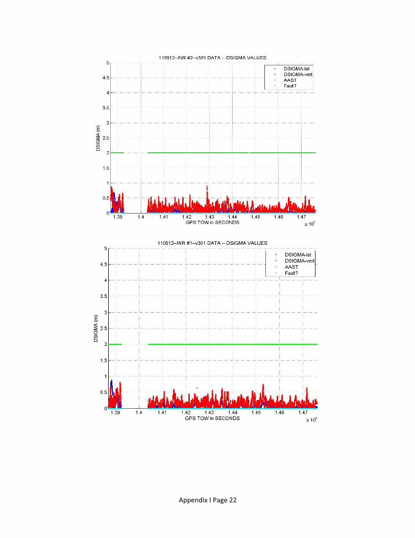
Plots below show the parameters for DSIGMA. Dv and Dl from two INRs run on the same flight are
plotted. There were no DSIGMA monitor failures. The Active Approach Service Type was initially GBAS
GAST D. The aircraft was out of PAR initially. As it moved IN PAR, the CCD monitor acted on both INRs
and they dropped to Autonomous Navigation mode. This is because the CCD filter output for all
measurements was higher than the threshold and it hadn’t passed the 20 minute observation period.
After that period, the receivers went to GAST D mode and dropped only when the aircraft was farther
than Dmax. This plot also shows whether the FD algorithm has found a measurement inconsistency in
the solution. No faults were detected in any flight tests.
Appendix I Page 22
Appendix I Page 23
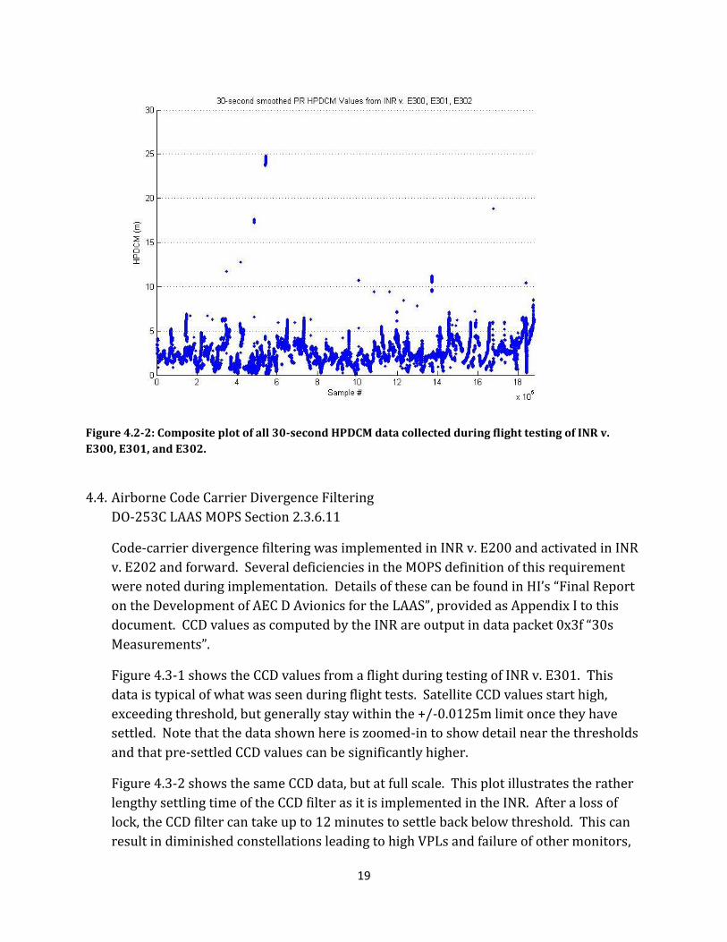
Plots below display the output of the HPDCM monitor. No failures were observed and HPDCM was much
below the threshold of 200 meters. The threshold is extremely high to ensure nothing but errors in VDB
data are caught by this monitor. This threshold was discussed in SC-159 and it was decided that DO-
253C contained the right value. At times, there can be some differences in the set of measurements
used by each INR. This can cause slight differences in HPDCM in the two INRs. Plot for INR #2 is on a
different scale to show the data point above 10m. Both INRs display a similar pattern.
Appendix I Page 24
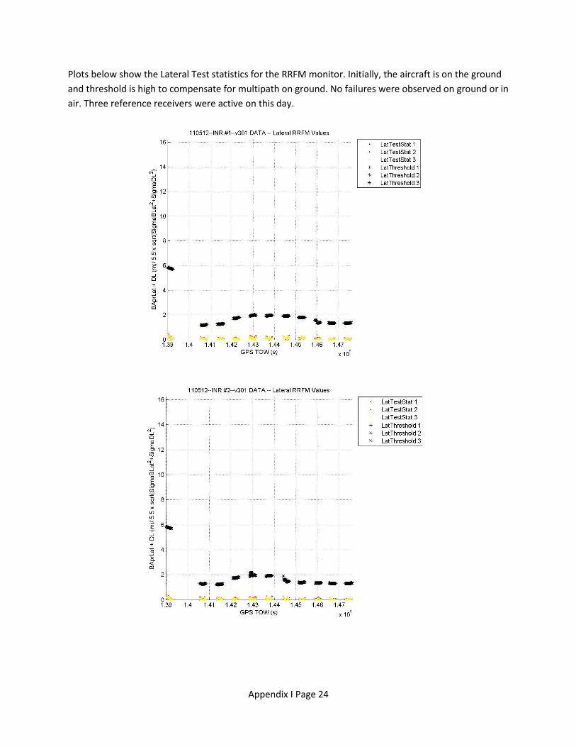
Plots below show the Lateral Test statistics for the RRFM monitor. Initially, the aircraft is on the ground
and threshold is high to compensate for multipath on ground. No failures were observed on ground or in
air. Three reference receivers were active on this day.
Appendix I Page 25
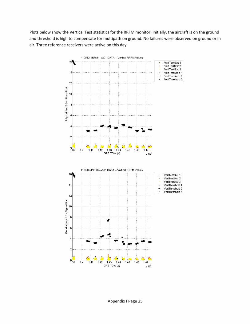
Plots below show the Vertical Test statistics for the RRFM monitor. Initially, the aircraft is on the ground
and threshold is high to compensate for multipath on ground. No failures were observed on ground or in
air. Three reference receivers were active on this day.
Appendix I Page 26
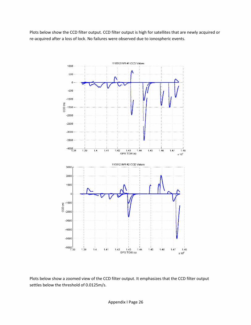
Plots below show the CCD filter output. CCD filter output is high for satellites that are newly acquired or
re-acquired after a loss of lock. No failures were observed due to ionospheric events.
Plots below show a zoomed view of the CCD filter output. It emphasizes that the CCD filter output
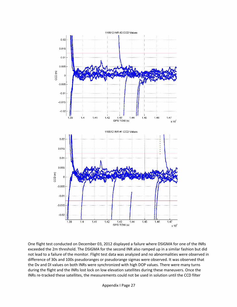
settles below the threshold of 0.0125m/s.
Appendix I Page 27
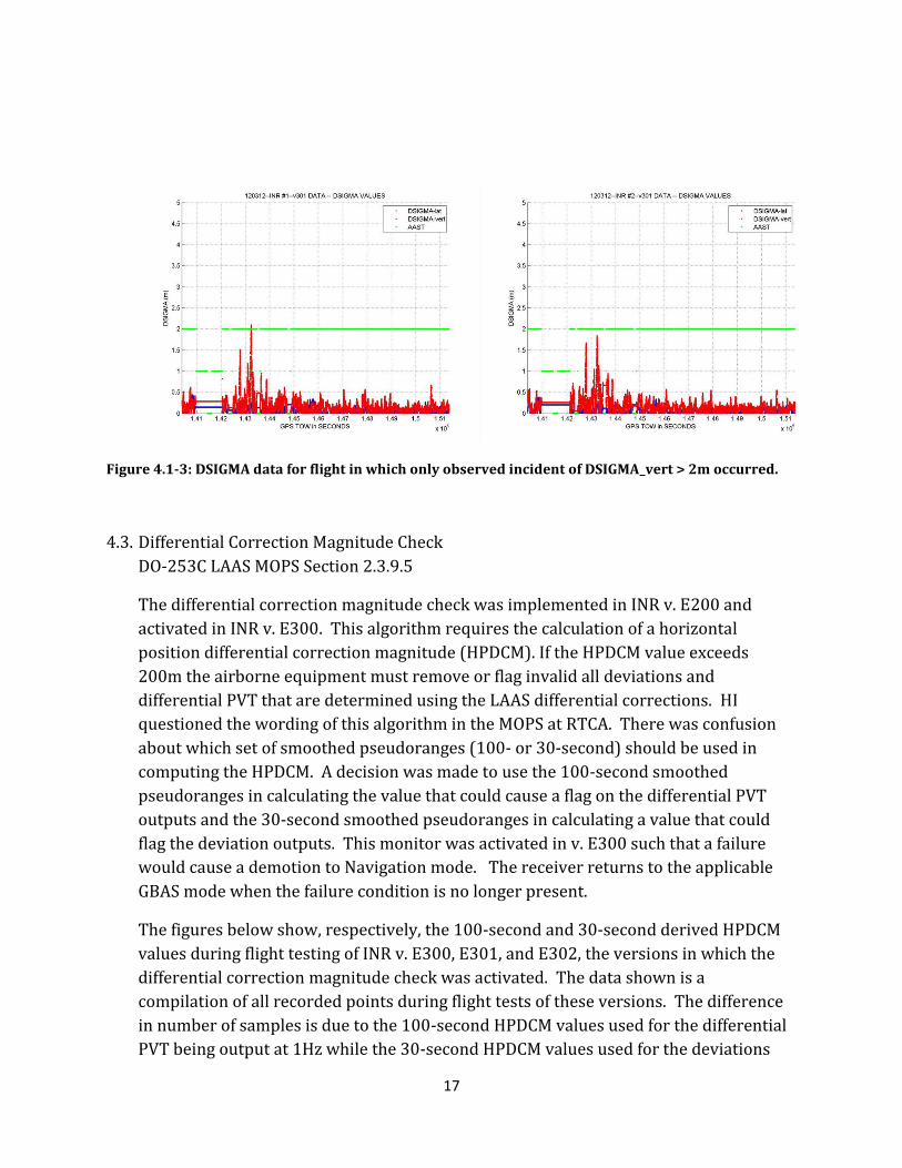
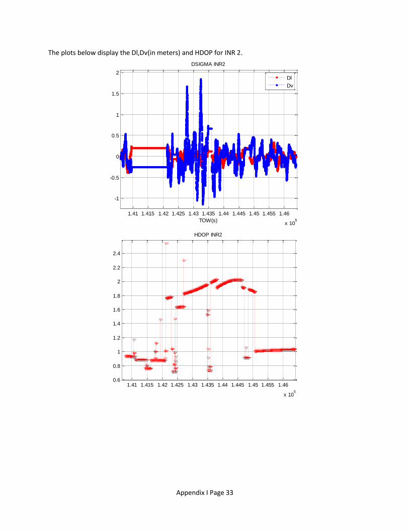
One flight test conducted on December 03, 2012 displayed a failure where DSIGMA for one of the INRs exceeded the 2m threshold. The DSIGMA for the second INR also ramped up in a similar fashion but did not lead to a failure of the monitor. Flight test data was analyzed and no abnormalities were observed in difference of 30s and 100s pseudoranges or pseudorange sigmas were observed. It was observed that the Dv and Dl values on both INRs were synchronized with high DOP values. There were many turns during the flight and the INRs lost lock on low elevation satellites during these maneuvers. Once the INRs re-tracked these satellites, the measurements could not be used in solution until the CCD filter
Appendix I Page 28
output for these measurements was above threshold, so the FD for SV addition algorithm could not allow them to be used in GBAS GAST D mode. Thus, delay in reusing lost measurements due to the high CCD filter output, led to a high DOP. This impacted the DSIGMA values. Following plots display these parameters on both INRs. The CCD filter defined in DO-253C takes a long time to settle. This has quite an impact on availability of satellites that were lost during turns and reacquired later. This monitor along with its impact on DSIGMA will be discussed with RTCA.
Appendix I Page 29
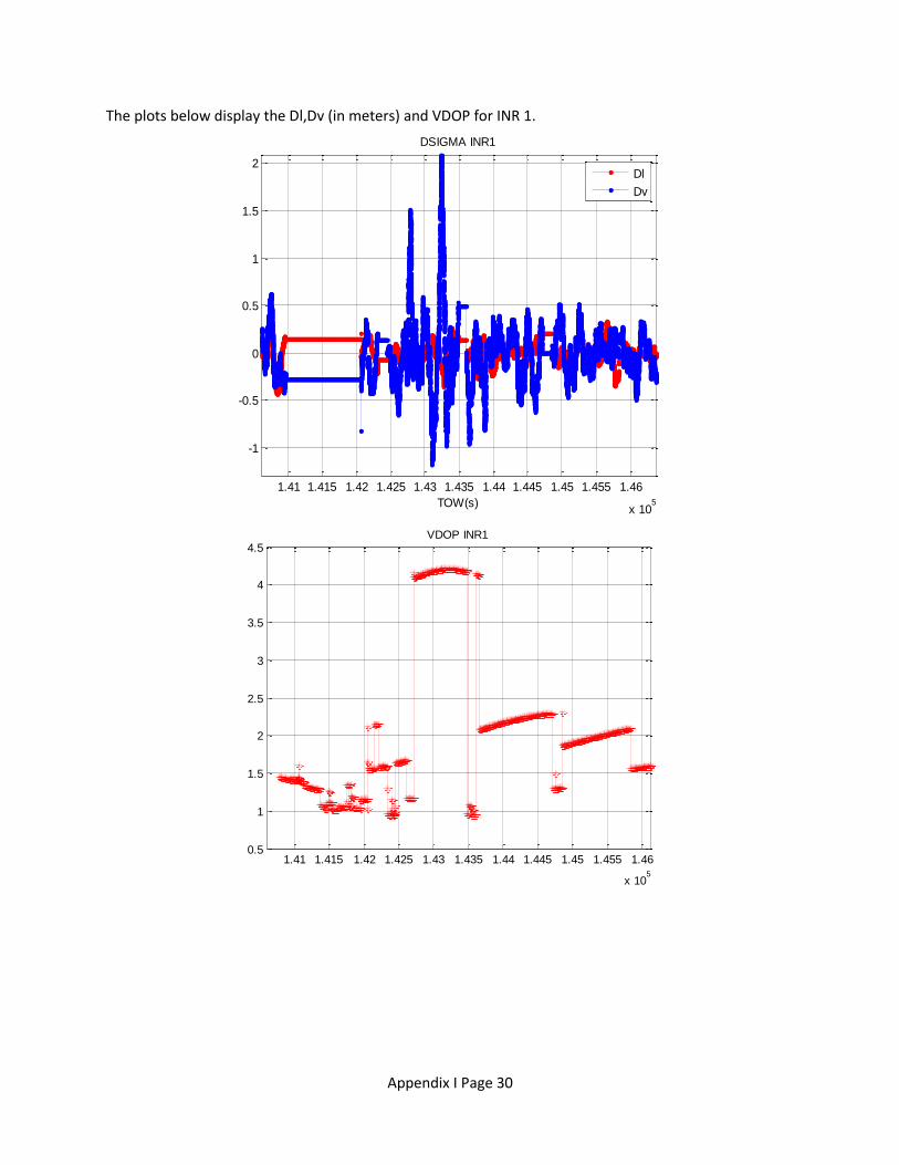
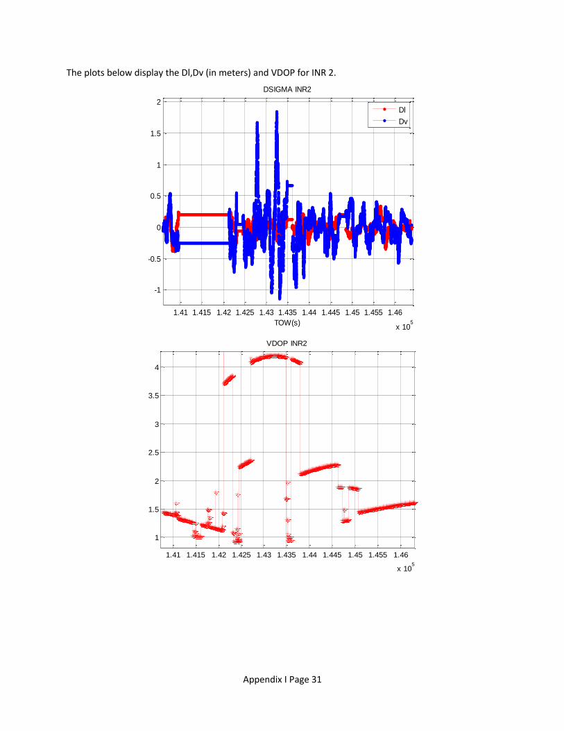
The plots below display the Dl,Dv and active Approach Service type for INR 1 and INR 2. It can be seen that both receivers follow the same pattern. INR1 fails DSIGMA as Dv went as high as 2.04m, while it went to 1.87m on INR2.
Appendix I Page 30
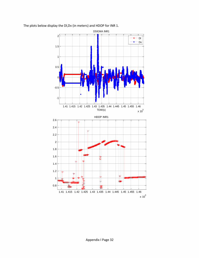
The plots below display the Dl,Dv (in meters) and VDOP for INR 1.
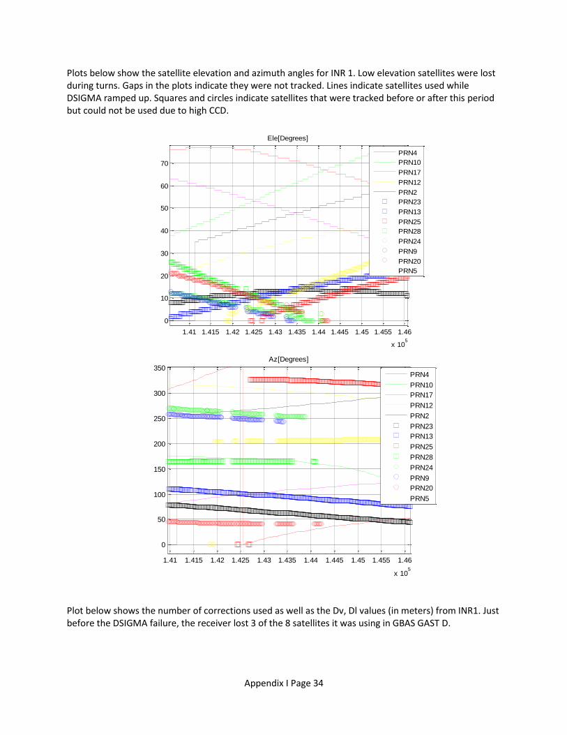
Plots below show the satellite elevation and azimuth angles for INR 1. Low elevation satellites were lost during turns. Gaps in the plots indicate they were not tracked. Lines indicate satellites used while DSIGMA ramped up. Squares and circles indicate satellites that were tracked before or after this period but could not be used due to high CCD.
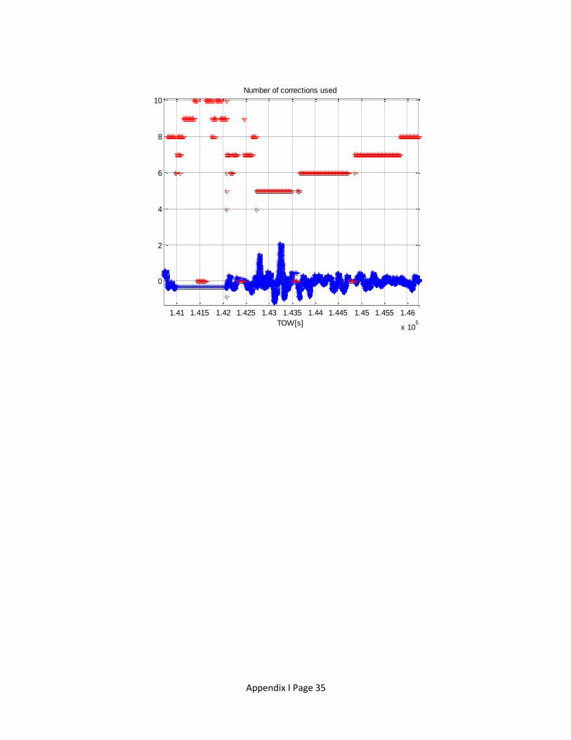
Plot below shows the number of corrections used as well as the Dv, Dl values (in meters) from INR1. Just before the DSIGMA failure, the receiver lost 3 of the 8 satellites it was using in GBAS GAST D.
Plot below shows the CCD filter output (in m/s) for satellites tracked by INR1. It can be seen that CCD filter was reset several times for some satellites. This synchronized with the turns. A plot showing change in the ground track is also displayed.
1.42 1.425 1.43 1.435 1.44 1.445
x 105
-250
-200
-150
-100
-50
0
50
100
150
200
CCD[m]
PRN4
PRN10
PRN17
PRN12
PRN2
PRN23
PRN13
PRN25
PRN28
PRN24
PRN9
PRN20
PRN5
1.42 1.425 1.43 1.435 1.44 1.445
x 105
-0.5
-0.4
-0.3
-0.2
-0.1
0
0.1
0.2
0.3
0.4
0.5
Change in ground track
Appendix I Page 37
Appendix A: Evaluation of GBAS fault detection performance