Gaussian Process Motion Planning

Mustafa Mukadam, Xinyan Yan, and Byron Boots

Abstract— Motion planning is a fundamental tool in robotics,used to generate collision-free, smooth, trajectories, while sat-isfying task-dependent constraints. In this paper, we present anovel approach to motion planning using Gaussian processes.In contrast to most existing trajectory optimization algorithms,which rely on a discrete state parameterization in practice,we represent the continuous-time trajectory as a sample froma Gaussian process (GP) generated by a linear time-varyingstochastic differential equation. We then provide a gradient-based optimization technique that optimizes continuous-timetrajectories with respect to a cost functional. By exploiting GPinterpolation, we develop the Gaussian Process Motion Planner(GPMP), that finds optimal trajectories parameterized by asmall number of states. We benchmark our algorithm againstrecent trajectory optimization algorithms by solving 7-DOFrobotic arm planning problems in simulation and validate ourapproach on a real 7-DOF WAM arm.

I. INTRODUCTION & RELATED WORK

Motion planning is a fundamental skill for robots thataspire to move through an environment without collisionor manipulate objects to achieve some goal. We considermotion planning from a trajectory optimization perspective,where we seek to find a trajectory that minimizes a givencost function while satisfying any given constraints.

A significant amount of previous work has focused ontrajectory optimization and related problems. Khatib [1]pioneered the idea of potential field where the goal position isan attractive pole and the obstacles form repulsive fields. Var-ious extensions have been proposed to address problems likelocal minimum [2], and ways of modeling the free space [3].Covariant Hamiltonian Optimization for Motion Planning(CHOMP) [4], [5] utilizes covariant gradient descent to min-imize obstacle and smoothness cost functionals, and a pre-computed signed distance field for fast collision checking.STOMP [6] is a stochastic trajectory optimization methodthat can work with non-differentiable constraints by samplinga series of noisy trajectories. An important drawback ofCHOMP and STOMP is that a large number of trajectorystates are needed to reason about small obstacles or findfeasible solutions when there are many constraints. MultigridCHOMP [7] attempts to reduce the computation time ofCHOMP when using a large number of states by startingwith a low-resolution trajectory and gradually increasing theresolution at each iteration. Finally, TrajOpt [8] formulatesmotion planning as sequential quadratic programming. Swept

Mustafa Mukadam, Xinyan Yan, and Byron Boots are affiliated withthe Institute for Robotics and Intelligent Machines, Georgia Instituteof Technology, Atlanta, GA 30332, USA. mmukadam3@gatech.edu{xinyan.yan,bboots}@cc.gatech.edu. This work was funded inpart by the National Science Foundation, grant number IIS-1464219.

volumes are considered to ensure continuous-time safety,enabling TrajOpt to solve more problems with fewer states.

In this paper, we present a novel Gaussian process (GP)approach to motion planning. Although, Gaussian processes[9] have been used for function approximation in many areasof robotics including supervised learning [10], [11], inversedynamics modeling [12], [13], reinforcement learning [14],path prediction [15], simultaneous localization and map-ping [16], [17], state estimation [18]–[20], and controls [21],to our knowledge they have not been used for motionplanning before.

GPs provide a very natural way to model motion planningproblems with several advantages over previous approaches.Vector-valued GPs provide a principled way to representcontinuous-time trajectories as functions that map time torobot states. Smooth trajectories can be represented com-pactly with only a small number of states, and Gaussianprocess regression can be used to query the state of the robotat any time of interest. Using this insight, we develop theGaussian Process Motion Planner (GPMP), a new motionplanning algorithm that optimizes trajectories parameterizedby a small number of states, using Gaussian process inter-polation and gradient-based optimization. We evaluate ouralgorithm both in simulation and on a 7-DOF Barrett WAMarm, and we benchmark our approach against several recenttrajectory optimization algorithms.

II. A GAUSSIAN PROCESS MODEL FORCONTINUOUS-TIME TRAJECTORIES

Motion planning traditionally involves finding a smooth,collision-free trajectory from a start state to a goal state.Similar to previous approaches [4]–[8], we treat motion plan-ning as an optimization problem and search for a trajectorythat minimizes a predefined cost function (Section III). Incontrast to these previous approaches, which consider finelydiscretized discrete time trajectories in practice, we considercontinuous-time trajectories such that the state at time t is

ξ(t) = {ξd(t)}Dd=1 ξd(t) = {ξdr(t)}Rr=1 (1)

where D is the dimension of the configuration space (numberof joints), and R is the number of variables in each config-uration dimension. Here we choose R = 3, specifying jointpositions, velocities, and accelerations, ensuring that ourstate is Markovian. Using the Markov property of the state inthe motion prior, defined in Eq. 6 below, allows us to buildan exactly sparse inverse kernel (precision matrix) [16], [22]useful for efficient optimization and fast GP interpolation(Section II-B).

Continuous-time trajectories are assumed to be sampledfrom a vector-valued Gaussian process (GP):

ξ(t) ∼ GP(µ(t),K(t, t′)) t0 < t, t′ < tN+1 (2)

where µ(t) is a vector-valued mean function whose com-ponents are the functions {µdr(t)}D,Rd=1,r=1 and the en-tries K(t, t′)dr,d′r′ in the matrix-valued covariance functionK(t, t′) corresponding to the covariances between ξdr(t) andξd′r′(t′). Based on the definition of vector-valued Gaussian

processes [23], any collection of N states on the trajectoryhas a joint Gaussian distribution,

ξ ∼ N (µ,K), ξ = ξ1:N , µ = µ1:N ,

Kij = K(ti, tj), t1 ≤ ti, tj ≤ tN(3)

The start and goal states, ξ0 and ξN+1, are excluded becausethey are fixed. ξi denotes the state at time ti.

Reasoning about trajectories with GPs has several advan-tages. The Gaussian process imposes a prior distributionon the space of trajectories. Given a fixed set of time-parameterized states, we can condition the GP on those statesto compute the posterior mean at any time of interest:

ξ(τ) = µ(τ) +K(τ)K−1(ξ − µ) (4)

K(τ) = [ K(τ, t1) . . . K(τ, tN )] (5)

A consequence of GP interpolation is that the trajectory doesnot need to be discretized at a high resolution, and trajectorystates do not need to be evenly spaced in time. Additionally,the posterior mean is the maximum a posteriori interpolationof the trajectory, and high-frequency interpolation can beused to generate an executable trajectory or reason about thecost over the entire trajectory instead of just at the states.

A. Gaussian Processes Generated by Linear Time-VaryingStochastic Differential Equations

The choice of prior is an important design considerationwhen working with Gaussian processes. In this work, weconsider the Gaussian processes generated by the linear timevarying (LTV) stochastic differential equations (SDEs) [16]:

ξ′(t) = A(t)ξ(t) + F (t)w(t)

w(t) ∼ GP(0, Qcδ(t− t′)), t0 < t, t′ < tN+1

(6)

where A(t) are F (t) are time-varying system matrices, δ(·)is the Dirac delta function, w(t) is the process noise modeledby a Gaussian process with zero mean, and Qc is a power-spectral density matrix, a hyperparameter that can be setusing data collected on the system [16].

Given the fixed start state ξ0 as the initial condition, andΦ(t, s), the state transition matrix that propagates the statefrom time s to t, the solution to the SDE is:

ξ(t) = Φ(t, t0)ξ0 +

∫ t

t0

Φ(t, s)F (s)w(s)ds (7)

ξ(t) corresponds to a Gaussian process. The mean functionand the covariance function can be obtained from the firstand second moments:

µ(t) = Φ(t, t0)ξ0 (8)

K(t, t′) = E[(ξ(t)− µ(t))(ξ(t′)− µ(t′))T ]

=

∫ min(t,t′)

t0

Φ(t, s)F (s)QcF (s)TΦ(t′, s)T ds(9)

After considering the end state ξN+1 as a noise-free “mea-surement”, and conditioning ξ(t) on this measurement, wederive the Gaussian process for the trajectories with fixedstart and end states. The mean and covariance functions are:

µ(t) = µt + KN+1,tK−1N+1,N+1(ξN+1 − µN+1) (10)

= Φt,0ξ0 +WtΦᵀN+1,tW

−1N+1 (ξN+1 − ΦN+1,0ξ0)

K(t, t′) = Kt,t′ − KᵀN+1,tK

−1N+1,N+1KN+1,t′ , t < t′ (11)

= WtΦᵀt′,t −WtΦ

ᵀN+1,tW

−1N+1ΦN+1,t′Wt′ , t < t′

where

Wt =

∫ t

t0

Φ(t, s)F (s)QcF (s)TΦ(t′, s)T ds (12)

The inverse kernel matrix K−1 for the N states is exactlysparse (block-tridiagonal), and can be factored as:

K−1 = BTQ−1B (13)

where

B =

1 0 . . . 0−Φ(t1, t0) 1 . . . 0

0 −Φ(t2, t1). . .

......

.... . . 1

0 0 . . . −Φ(tN , tN−1)

(14)

and

Q = diag(Q1, ..., QN+1),

Qi =

∫ ti

ti−1

Φ(ti, s)F (s)QcF (s)TΦ(ti, s)T ds

Here Q−1 is block diagonal, and B is band diagonal.The inverse kernel matrix, K−1, encodes constraints on

consecutive states imposed by the state transition matrix,Φ(t, s). If state ξ(t) includes joint angles, velocities, andaccelerations, then the constraints are on all of these vari-ables. If we take this state transition matrix and Q−1 to beunit scalars, then K−1 reduces to the matrix A formed byfinite differencing in CHOMP [4].

B. Fast Gaussian Process Interpolation

An advantage of Gaussian process trajectory estimationis that any point on a trajectory can be interpolated fromother points by computing the posterior mean (Eq. 4). Inthe case of a GP generated from the LTV-SDE in Sec. II-A,interpolation is very fast, involving only two nearby statesand is performed in O(1) time [16]:

ξ(τ) = µ(τ) + [ Λ(τ) Ψ(τ) ]

([ξiξi+1

]−[

µiµi+1

])(15)

where ti < τ < ti+1, i = 0, ..., N . This is because only the(i)th and (i+1)th block columns of K(τ)K−1 are non-zero:

K(τ)K−1 = [ 0 . . . 0 Λ(τ) Ψ(τ) 0 . . . 0 ] (16)

where Λ(τ) = Φ(τ, ti) − Ψ(τ)Φ(ti+1, ti), and Ψ(τ) =QτΦ(τ, ti)

TQ−1i+1. We make use of this fast interpolation

during optimization (Section III-D).

III. CONTINUOUS-TIME MOTION PLANNING WITHGAUSSIAN PROCESSES

Motion planning can be viewed as the following problem:

minimize U [ξ] (17)subject to fi[ξ] ≤ 0, i = 1, ...,m

where the trajectory ξ is a continuous-time function withstart and end states fixed, U [ξ] is an objective or costfunctional that evaluates the quality of a trajectory, andfi[ξ] are constraint functionals such as joint limits and task-dependent constraints. For simplicity of notation, we use ξ torepresent either the continuous-time function or the N statesthat parameterize the function (Eq. 3). Its meaning should beclear from context. Functionals take their function argumentsin brackets, for example U [ξ].

A. Cost Functionals

The usual goal of trajectory optimization is to find trajec-tories that are smooth and collision free. Therefore, we definethe objective functional as a combination of two objectives:a prior functional, Fgp, determined by the Gaussian processprior that penalizes the displacement of the trajectory fromthe prior mean to keep the trajectory smooth, and an obstaclecost functional, Fobs, that penalizes collision with obstacles.Thus the objective functional is

U [ξ] = Fobs[ξ] + λFgp[ξ] (18)

where the tradeoff between the two functionals is controlledby λ. This objective functional looks similar to the one usedin CHOMP [4], however, in our case the trajectory alsocontains velocities and accelerations. Another important dis-tinction is that the smoothness cost in CHOMP is calculatedfrom finite dynamics while here it is generated from the GPprior.

The prior functional Fgp is induced by the GP formulationin Eq. 2:

Fgp[ξ] =1

2‖ξ − µ‖2K (19)

where the norm is the Mahalanobis norm: ‖e‖2Σ = eᵀΣ−1e.We use an obstacle cost functional Fobs similar to the

one used in CHOMP [4], [5], that computes the arc-lengthparameterized line integral of the workspace obstacle costof each body point as it passes through the workspace, andintegrates over all body points:

Fobs[ξ] =

∫B

∫ tN+1

t0

c(x)||x′|| dt du

=

∫ tN+1

t0

∫Bc(x)||x′|| du dt

(20)

where B ⊂ R3 is the set of points on the robot body,x(·) : C × B → R3 is the forward kinematics that mapsrobot configuration q to workspace, and c(·) : R3 → R is

the workspace cost function that penalizes the body pointswhen they are in or around an obstacle. In practice, this iscalculated using a precomputed signed distance field. x′ isthe velocity of a body point in workspace. Multiplying thenorm of the velocity to the cost in the line integral abovegives an arc-length parameterization that is invariant to re-timing the trajectory. Intuitively, this encourages trajectoriesto minimize cost by circumventing obstacles rather thanattempting to pass through them very quickly.

B. Optimization

Optimizing the objective functional U [ξ] in Eq. 18 can bequite difficult since the cost Fobs is non-convex. We adopt aniterative, gradient-based approach to minimize U [ξ]. At eachiteration we form an approximation to the cost functional viaa Taylor series expansion around the current trajectory ξ:

U [ξ] ≈ U [ξ] + ∇U [ξ](ξ − ξ) (21)

We then minimize the approximate cost while constrainingthe trajectory to be close to the previous one. The optimalperturbation δξ∗ to the trajectory is:

δξ∗ = argminδξ

{U [ξ] + ∇U [ξ](ξ − ξ) +

η

2‖ξ − ξ‖2K

}= argmin

δξ

{U [ξ] + ∇U [ξ]δξ +

η

2‖δξ‖2K

} (22)

where η is the regularization constant. Eq. 22 can be solvedby differentiating the right-hand side and setting the resultto zero:

∇U [ξ] + ηK−1δξ∗ = 0 =⇒ δξ∗ = −1

ηK∇U [ξ] (23)

At each iteration, the update rule is therefore

ξ ← ξ + δξ∗ = ξ − 1

ηK∇U [ξ] (24)

To complete the update, we need to compute the gradient ofthe cost functional ∇U [ξ] at the current trajectory ξ, whichrequires finding ∇Fgp and ∇Fobs:

∇U [ξ] = ∇Fobs + λ∇Fgp (25)

We discuss the two component gradients below.1) Gradient of the Prior Cost: The cost functional Fgp

can be viewed as penalizing trajectories that deviate froma prescribed motion model. An example is given in Eq. 37in the Experimental Results (Section IV). To compute thegradient of the prior cost, we first expand Eq. 19:

Fgp[ξ] =1

2(ξT − µT )K−1(ξ − µ)

=1

2ξTK−1ξ − µTK−1ξ +

1

2µTK−1µ

(26)

and then take the derivative with respect to the trajectory ξ

∇Fgp[ξ] = K−1ξ −K−1µ = K−1(ξ − µ) (27)

2) Gradient of Obstacle Cost: The functional gradient ofthe obstacle cost Fobs in Eq. 20 can be computed from theEuler-Lagrange equation [24] in which a functional of theform F [ξ] =

∫v(ξ)dt yields a gradient

∇F [ξ] =∂v

∂ξ− d

dt

∂v

∂ξ′(28)

Applying Eq. 28 to find the gradient of Eq. 20 in theworkspace and then mapping it back to the configurationspace via the kinematic Jacobian [25], and following theproof in [26], we compute the gradient with respect toposition, velocity, and acceleration as

∇Fobs[ξ] =

∫B J

T ||x′||[(I − x′x′T )∇c− cκ

]du∫

B JT c x′du

0

(29)

where κ = ||x′||−2(I − x′x′T )x′′ is the curvature vectoralong workspace trajectory traced by a body point, x′, x′′ arethe velocity and acceleration of that body point determinedby forward kinematics and the Hessian, x′ = x′/||x′||is the normalized velocity vector, and J is the kinematicJacobian of that body point. CHOMP uses finite differencingto calculate x′ and x′′, but with our representation of the state(Eq. 1), x′ and x′′ can be obtained directly from the Jacobianand Hessian respectively, since velocities and accelerationsin configuration space are a part of the state.

C. Update Rule

In order to compute the gradient of prior and obstaclefunctionals, we parameterize the continuous-time trajectoryby a small, N number of states, ξ = ξ1:N . If we consider GPsgenerated by LTV-SDEs, as in Sec. II-A, then the GP priorcost Fgp(ξ) can be computed from the observed states basedon the expression of the inverse kernel matrix in Eq. 13.Using B in Eq. 14, and µ(t) in Eq. 10:

Fgp(ξ) =1

2‖ξ − µ‖2K =

1

2‖B(ξ − µ)‖2Q

=1

2

N∑i=1

‖Φ(ti, ti−1)ξi−1 − ξi‖2Qi(30)

∇Fgp(ξ) = K−1(ξ − µ) = BTQ−1B(ξ − µ) (31)

The gradient of the obstacle cost is calculated at the N states.In practice ∇Fobs(ξ) is further approximated by summing upthe gradients with regard to a finite number of body pointsof the robot B′ ⊂ B. So the obstacle gradient becomes:

∇ξiFobs(ξ) =

∑′B J

Ti ||x′i||

[(I − x′ix′Ti )∇ci − ciκi

]du∑′

B JTi ci x

′idu

0

(32)

where i denotes the value of the symbol at time ti.

The update rule for states can be summarized fromEqs. 24, 25, and 27 as:

ξ ← ξ − 1

ηK

[λK−1(ξ − µ) + g

](33)

where g is a vector of obstacle gradients at each state(Eq.32). Note that this update rule can be interpreted asa generalization of the update rule for CHOMP, but witha trajectory of states that have been augmented to includevelocities and accelerations. Thus, we will refer to thisalgorithm as Augmented CHOMP (AugCHOMP). In thenext sub-section we fully leverage the GP prior and GPinterpolation machinery to generalize the motion planningalgorithm further.

D. Compact Trajectory Representations and Faster Updatesvia Gaussian Process Interpolation

A key benefit of Gaussian process motion planning overfixed, discrete state parameterizations of trajectories, is thatwe can use the GP to query the trajectory function at anytime of interest (see Section II-B). To interpolate p pointsbetween two states i and i + 1, we define two aggregatedmatrices:

Λi =[

ΛTi,1 . . . ΛTi,j . . . ΛTi,p]T

Ψi =[

ΨTi,1 . . . ΨT

i,j . . . ΨTi,p

]T (34)

For example, if we want to upsample a trajectory by inter-polating p points between each two trajectory states, we canquickly compute the new trajectory as

ξ = M(ξw − µw) + µ (35)

where, M =

Ψ0 0 . . . . . . . . . . . . 0 0I 0 . . . . . . . . . . . . 0 0

Λ1 Ψ1 . . . . . . . . . . . . 0 00 I . . . . . . . . . . . . 0 0...

.... . .

......

0 0 . . . I 0 . . . 0 00 0 . . . Λi Ψi . . . 0 00 0 . . . 0 I . . . 0 0...

.... . .

......

0 0 . . . . . . . . . . . . 0 I0 0 . . . . . . . . . . . . 0 ΛN

ξw is the trajectory with a sparse set of states. Fast, hightemporal-resolution interpolation is useful in practice if wewant to feed the planned trajectory into a controller, or if wewant to carefully check for collisions between states duringoptimization.

GP interpolation additionally allows us to reduce the num-ber of states needed to represent a high-fidelity continuous-time trajectory, as compared with the discrete-state formula-tion of CHOMP, resulting in a speedup during optimizationwith virtually no effect on the final plan. The idea is tomodify Eq. 33 to update only a sparse set of states ξw, butsweep through the full trajectory to compute the obstaclecost by interpolating a large number of intermediate points.The obstacle gradient is calculated for all points (interpolated

(a) (b) (c) (d)

Fig. 1: (a) Environment with 4 start robot arm configurations (on the table) and 6 end robot arm configurations (on thecabinet shelves) used to generate a set of 24 unique planning problems. These planning problems entail displacing objectsfrom the table to the cabinet shelves. The plans are generated in OpenRAVE and executed on the real robot. (b) Exampleof a successful plan generated by GPMP on one of the planning problems. This plan is used to move a milk bottle fromthe table to a shelf in the cabinet in (c) simulation and (d) on the real WAM robot.

points and states) and then projected back onto just the statesusing the matrix MT (see Eq. 36 below). The update rulefor this approach is derived from Eq. 33 as

ξ ← ξ − 1

ηK[λK−1(ξ − µ) + g

]=⇒ Mξw ←Mξw−

1

ηMKwMT

[λM−TK−1

w M−1M(ξw − µw) + g

]=⇒ ξw ← ξw −

1

ηKw[λK−1

w (ξw − µw) +MT g

](36)

where Kw is the kernel and µw is the mean of the trajectoryξw with sparse set of states. We refer to this algorithm asthe Gaussian Process Motion Planner (GPMP).

IV. EXPERIMENTAL RESULTS

We benchmarked GPMP against CHOMP, AugCHOMP,STOMP, and TrajOpt by optimizing trajectories in Open-RAVE [27], a standard simulator used in motion planning [4],[5], [8], [28]–[31], and validated the resulting trajectorieson a real robot arm. Our experimental setup consisted of atable and a cabinet and a 7-DOF Barrett WAM arm whichwas initialized in several distinct configurations. Figure 1 (a)shows the start and end configurations of 24 unique planningproblems on which all the algorithms are tested.

For GPMP and AugCHOMP we employed a constant-acceleration prior, i.e. white-noise-on-jerk model, q′′′(t) =w(t). (Recall that w(t) is the process noise, see Eq. 6). Forsimplicity we assumed independence between the degrees offreedom (joints) of the robot. Following the form of LTV-SDE in Eq. 6 we specified the transition function of any jointd ∈ D,

Φd(t, s) =

1 (t− s) 12 (t− s)2

0 1 (t− s)0 0 1

(37)

With the independence assumption, it follows that Φ(t, s) =diag(Φ1(t, s), . . . ,ΦD(t, s)), and for all the states at ti, i =1 . . . N + 1 we compute

Qdi =

12∆t5iQc

18∆t4iQc

16∆t3iQc

18∆t4iQc

13∆t3iQc

12∆t2iQc

16∆t3iQc

12∆t2iQc ∆tiQc

,

(Qdi )−1 =

720∆t−5i Q−1

c −360∆t−4i Q−1

c 60∆t−3i Q−1

c

−360∆t−4i Q−1

c 192∆t−3i Q−1

c −36∆t−2i Q−1

c

60∆t−3i Q−1

c −36∆t−2i Q−1

c 9∆t−1i Q−1

c

(38)

where ∆ti = ti − ti−1. Similarly we compute Qi =diag(Q1

i , . . . , QDi ) and Q−1

i = diag((Q1i )−1, . . . , (QDi )−1).

The matrix Q−1 (Eq. 13) can be built directly and efficientlyfrom the Q−1

i s.Both GPMP and AugCHOMP handle constraints (Eq 17)

in the same way as CHOMP. For AugCHOMP joint limitsare obeyed by finding a violation trajectory ξv , calculated bytaking each point on the trajectory in violation and bringingit within joint limits via a L1 projection. It is then scaled bythe kernel such that it cancels out the largest violation in thetrajectory (see [5] for details),1

ξ = ξ +Kξv (39)

Joint limits for GPMP are obeyed using a technique similarto Eq. 36 applied to Eq. 39,

ξw = ξw +KwMT ξv (40)

For all algorithms except GPMP and AugCHOMP, trajecto-ries were initialized as a straight line in configuration space.For GPMP and AugCHOMP we found that initializing thetrajectory as a acceleration-smooth line yielded lower priorcost at the start. The initialized trajectories were parameter-ized by 103 equidistant states. For GPMP 18 states were usedwith p = 5 (103 states effectively), where p is a parameterthat represents the number of points interpolated betweenany two states during each iteration.

1For simplicity only positions in configuration space are considered whilecalculating ξv .

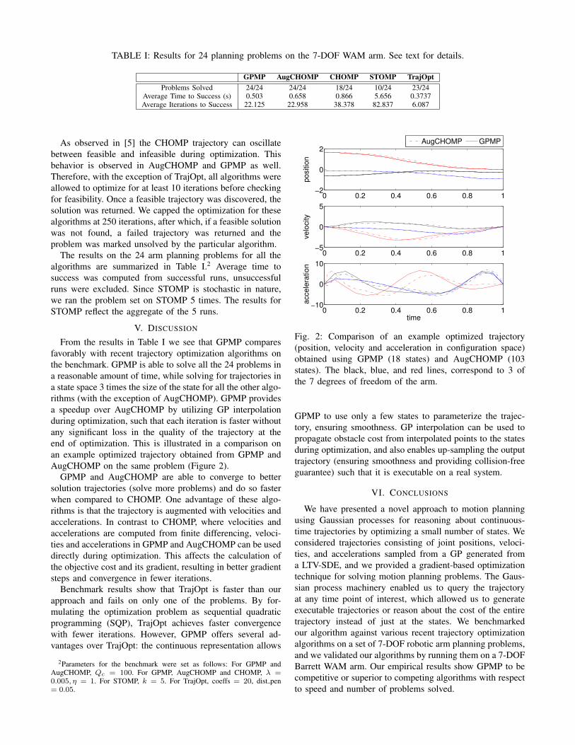
TABLE I: Results for 24 planning problems on the 7-DOF WAM arm. See text for details.

GPMP AugCHOMP CHOMP STOMP TrajOptProblems Solved 24/24 24/24 18/24 10/24 23/24

Average Time to Success (s) 0.503 0.658 0.866 5.656 0.3737Average Iterations to Success 22.125 22.958 38.378 82.837 6.087

As observed in [5] the CHOMP trajectory can oscillatebetween feasible and infeasible during optimization. Thisbehavior is observed in AugCHOMP and GPMP as well.Therefore, with the exception of TrajOpt, all algorithms wereallowed to optimize for at least 10 iterations before checkingfor feasibility. Once a feasible trajectory was discovered, thesolution was returned. We capped the optimization for thesealgorithms at 250 iterations, after which, if a feasible solutionwas not found, a failed trajectory was returned and theproblem was marked unsolved by the particular algorithm.

The results on the 24 arm planning problems for all thealgorithms are summarized in Table I.2 Average time tosuccess was computed from successful runs, unsuccessfulruns were excluded. Since STOMP is stochastic in nature,we ran the problem set on STOMP 5 times. The results forSTOMP reflect the aggregate of the 5 runs.

V. DISCUSSION

From the results in Table I we see that GPMP comparesfavorably with recent trajectory optimization algorithms onthe benchmark. GPMP is able to solve all the 24 problems ina reasonable amount of time, while solving for trajectories ina state space 3 times the size of the state for all the other algo-rithms (with the exception of AugCHOMP). GPMP providesa speedup over AugCHOMP by utilizing GP interpolationduring optimization, such that each iteration is faster withoutany significant loss in the quality of the trajectory at theend of optimization. This is illustrated in a comparison onan example optimized trajectory obtained from GPMP andAugCHOMP on the same problem (Figure 2).

GPMP and AugCHOMP are able to converge to bettersolution trajectories (solve more problems) and do so fasterwhen compared to CHOMP. One advantage of these algo-rithms is that the trajectory is augmented with velocities andaccelerations. In contrast to CHOMP, where velocities andaccelerations are computed from finite differencing, veloci-ties and accelerations in GPMP and AugCHOMP can be useddirectly during optimization. This affects the calculation ofthe objective cost and its gradient, resulting in better gradientsteps and convergence in fewer iterations.

Benchmark results show that TrajOpt is faster than ourapproach and fails on only one of the problems. By for-mulating the optimization problem as sequential quadraticprogramming (SQP), TrajOpt achieves faster convergencewith fewer iterations. However, GPMP offers several ad-vantages over TrajOpt: the continuous representation allows

2Parameters for the benchmark were set as follows: For GPMP andAugCHOMP, Qc = 100. For GPMP, AugCHOMP and CHOMP, λ =0.005, η = 1. For STOMP, k = 5. For TrajOpt, coeffs = 20, dist pen= 0.05.

0 0.2 0.4 0.6 0.8 1−2

0

2

positio

n

0 0.2 0.4 0.6 0.8 1−5

0

5

velo

city

0 0.2 0.4 0.6 0.8 1−10

0

10

time

accele

ration

AugCHOMP GPMP

Fig. 2: Comparison of an example optimized trajectory(position, velocity and acceleration in configuration space)obtained using GPMP (18 states) and AugCHOMP (103states). The black, blue, and red lines, correspond to 3 ofthe 7 degrees of freedom of the arm.

GPMP to use only a few states to parameterize the trajec-tory, ensuring smoothness. GP interpolation can be used topropagate obstacle cost from interpolated points to the statesduring optimization, and also enables up-sampling the outputtrajectory (ensuring smoothness and providing collision-freeguarantee) such that it is executable on a real system.

VI. CONCLUSIONS

We have presented a novel approach to motion planningusing Gaussian processes for reasoning about continuous-time trajectories by optimizing a small number of states. Weconsidered trajectories consisting of joint positions, veloci-ties, and accelerations sampled from a GP generated froma LTV-SDE, and we provided a gradient-based optimizationtechnique for solving motion planning problems. The Gaus-sian process machinery enabled us to query the trajectoryat any time point of interest, which allowed us to generateexecutable trajectories or reason about the cost of the entiretrajectory instead of just at the states. We benchmarkedour algorithm against various recent trajectory optimizationalgorithms on a set of 7-DOF robotic arm planning problems,and we validated our algorithms by running them on a 7-DOFBarrett WAM arm. Our empirical results show GPMP to becompetitive or superior to competing algorithms with respectto speed and number of problems solved.

REFERENCES

[1] O. Khatib, “Real-time obstacle avoidance for manipulators and mobilerobots,” The international journal of robotics research, vol. 5, no. 1,pp. 90–98, 1986.

[2] M. Mabrouk and C. McInnes, “Solving the potential field local mini-mum problem using internal agent states,” Robotics and AutonomousSystems, vol. 56, no. 12, pp. 1050–1060, 2008.

[3] J.-H. Chuang and N. Ahuja, “An analytically tractable potential fieldmodel of free space and its application in obstacle avoidance,” Systems,Man, and Cybernetics, Part B: Cybernetics, IEEE Transactions on,vol. 28, no. 5, pp. 729–736, 1998.

[4] N. Ratliff, M. Zucker, J. A. Bagnell, and S. Srinivasa, “CHOMP:Gradient optimization techniques for efficient motion planning,” inRobotics and Automation, 2009. ICRA’09. IEEE International Con-ference on. IEEE, 2009, pp. 489–494.

[5] M. Zucker, N. Ratliff, A. D. Dragan, M. Pivtoraiko, M. Klingensmith,C. M. Dellin, J. A. Bagnell, and S. S. Srinivasa, “CHOMP: CovariantHamiltonian optimization for motion planning,” The InternationalJournal of Robotics Research, vol. 32, no. 9-10, pp. 1164–1193, 2013.

[6] M. Kalakrishnan, S. Chitta, E. Theodorou, P. Pastor, and S. Schaal,“STOMP: Stochastic trajectory optimization for motion planning,” inRobotics and Automation (ICRA), 2011 IEEE International Conferenceon. IEEE, 2011, pp. 4569–4574.

[7] K. He, E. Martin, and M. Zucker, “Multigrid CHOMP with localsmoothing,” in Proc. of 13th IEEE-RAS Int. Conference on HumanoidRobots (Humanoids), 2013.

[8] J. Schulman, J. Ho, A. Lee, I. Awwal, H. Bradlow, and P. Abbeel,“Finding locally optimal, collision-free trajectories with sequentialconvex optimization.” in Robotics: Science and Systems, vol. 9, no. 1.Citeseer, 2013, pp. 1–10.

[9] C. E. Rasmussen, Gaussian processes for machine learning. Citeseer,2006.

[10] S. Vijayakumar, A. D’souza, and S. Schaal, “Incremental onlinelearning in high dimensions,” Neural computation, vol. 17, no. 12,pp. 2602–2634, 2005.

[11] K. Kersting, C. Plagemann, P. Pfaff, and W. Burgard, “Most likelyheteroscedastic Gaussian process regression,” in Proceedings of the24th international conference on Machine learning. ACM, 2007, pp.393–400.

[12] D. Nguyen-Tuong, J. Peters, M. Seeger, and B. Scholkopf, “Learninginverse dynamics: a comparison,” in European Symposium on ArtificialNeural Networks, no. EPFL-CONF-175477, 2008.

[13] J. Sturm, C. Plagemann, and W. Burgard, “Body schema learningfor robotic manipulators from visual self-perception,” Journal ofPhysiology-Paris, vol. 103, no. 3, pp. 220–231, 2009.

[14] M. Deisenroth and C. E. Rasmussen, “PILCO: A model-based anddata-efficient approach to policy search,” in Proceedings of the 28thInternational Conference on machine learning (ICML-11), 2011, pp.465–472.

[15] M. K. C. Tay and C. Laugier, “Modelling smooth paths using Gaussian

processes,” in Field and Service Robotics. Springer, 2008, pp. 381–390.

[16] T. Barfoot, C. H. Tong, and S. Sarkka, “Batch continuous-timetrajectory estimation as exactly sparse Gaussian process regression,”Proceedings of Robotics: Science and Systems, Berkeley, USA, 2014.

[17] X. Yan, V. Indelman, and B. Boots, “Incremental sparse GP regressionfor continuous-time trajectory estimation & mapping,” in Proceedingsof the International Symposium on Robotics Research (ISRR-2015),2015.

[18] J. Ko and D. Fox, “GP-BayesFilters: Bayesian filtering using Gaussianprocess prediction and observation models,” Autonomous Robots,vol. 27, no. 1, pp. 75–90, 2009.

[19] J. Ko, D. J. Klein, D. Fox, and D. Haehnel, “GP-UKF: UnscentedKalman filters with Gaussian process prediction and observation mod-els,” in Intelligent Robots and Systems, 2007. IROS 2007. IEEE/RSJInternational Conference on. IEEE, 2007, pp. 1901–1907.

[20] C. H. Tong, P. Furgale, and T. D. Barfoot, “Gaussian process Gauss-Newton: Non-parametric state estimation,” in Computer and RobotVision (CRV), 2012 Ninth Conference on. IEEE, 2012, pp. 206–213.

[21] E. Theodorou, Y. Tassa, and E. Todorov, “Stochastic differential dy-namic programming,” in American Control Conference (ACC), 2010.IEEE, 2010, pp. 1125–1132.

[22] M. R. Walter, R. M. Eustice, and J. J. Leonard, “Exactly sparse ex-tended information filters for feature-based SLAM,” The InternationalJournal of Robotics Research, vol. 26, no. 4, pp. 335–359, 2007.

[23] M. A. Alvarez, L. Rosasco, and N. D. Lawrence, “Kernels for vector-valued functions: A review,” arXiv preprint arXiv:1106.6251, 2011.

[24] R. Courant and D. Hilbert, Methods of mathematical physics. CUPArchive, 1966, vol. 1.

[25] N. Ratliff, “Analytical dynamics and contact analysis,” Available:http://ipvs.informatik.uni-stuttgart.de.

[26] S. Quinlan, “Real-time modification of collision-free paths,” Ph.D.dissertation, Stanford University, 1994.

[27] R. Diankov and J. Kuffner, “Openrave: A planning architecture forautonomous robotics,” Robotics Institute, Pittsburgh, PA, Tech. Rep.CMU-RI-TR-08-34, vol. 79, 2008.

[28] A. Byravan, B. Boots, S. S. Srinivasa, and D. Fox, “Space-timefunctional gradient optimization for motion planning,” in Robotics andAutomation (ICRA), 2014 IEEE International Conference on. IEEE,2014, pp. 6499–6506.

[29] M. R. Dogar and S. S. Srinivasa, “Push-grasping with dexterous hands:Mechanics and a method,” in Intelligent Robots and Systems (IROS),2010 IEEE/RSJ International Conference on. IEEE, 2010, pp. 2123–2130.

[30] A. D. Dragan, N. D. Ratliff, and S. S. Srinivasa, “Manipulationplanning with goal sets using constrained trajectory optimization,” inRobotics and Automation (ICRA), 2011 IEEE International Conferenceon. IEEE, 2011, pp. 4582–4588.

[31] L. Y. Chang, S. S. Srinivasa, and N. S. Pollard, “Planning pre-graspmanipulation for transport tasks,” in Robotics and Automation (ICRA),2010 IEEE International Conference on. IEEE, 2010, pp. 2697–2704.