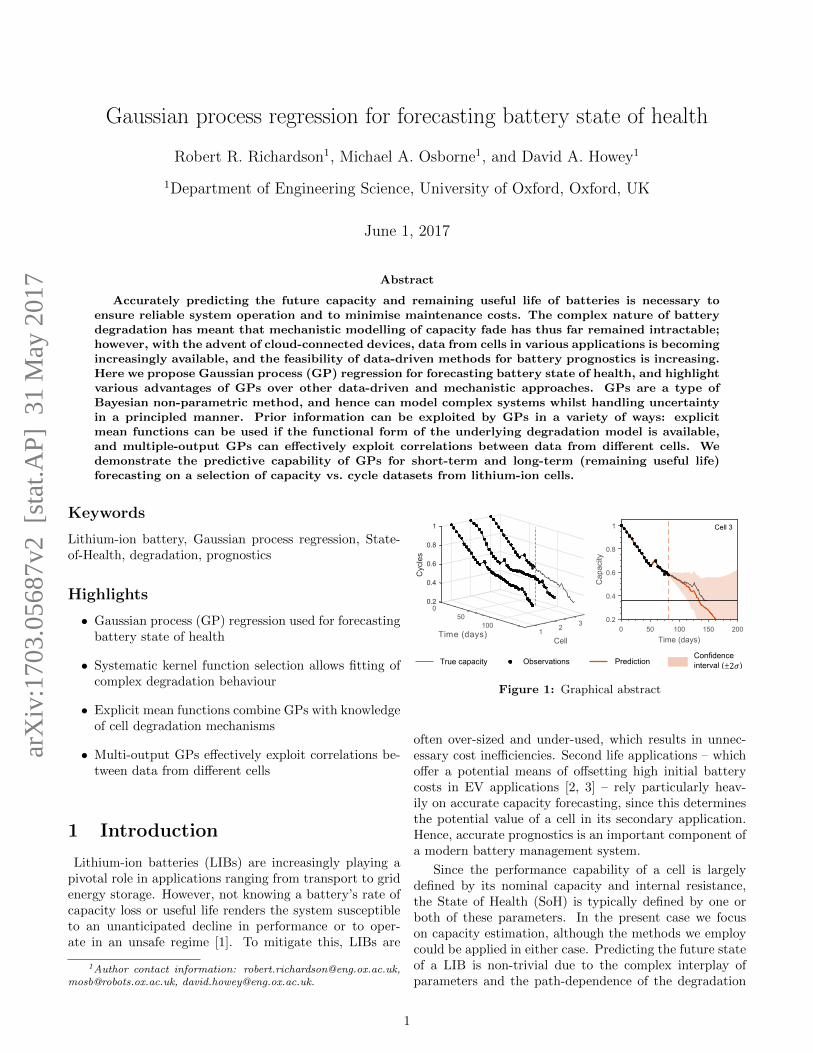
Gaussian process regression for forecasting battery state of health

Robert R. Richardson1, Michael A. Osborne1, and David A. Howey1

1Department of Engineering Science, University of Oxford, Oxford, UK

June 1, 2017

Abstract

Accurately predicting the future capacity and remaining useful life of batteries is necessary toensure reliable system operation and to minimise maintenance costs. The complex nature of batterydegradation has meant that mechanistic modelling of capacity fade has thus far remained intractable;however, with the advent of cloud-connected devices, data from cells in various applications is becomingincreasingly available, and the feasibility of data-driven methods for battery prognostics is increasing.Here we propose Gaussian process (GP) regression for forecasting battery state of health, and highlightvarious advantages of GPs over other data-driven and mechanistic approaches. GPs are a type ofBayesian non-parametric method, and hence can model complex systems whilst handling uncertaintyin a principled manner. Prior information can be exploited by GPs in a variety of ways: explicitmean functions can be used if the functional form of the underlying degradation model is available,and multiple-output GPs can effectively exploit correlations between data from different cells. Wedemonstrate the predictive capability of GPs for short-term and long-term (remaining useful life)forecasting on a selection of capacity vs. cycle datasets from lithium-ion cells.

Keywords

Lithium-ion battery, Gaussian process regression, State-of-Health, degradation, prognostics

Highlights

• Gaussian process (GP) regression used for forecastingbattery state of health

• Systematic kernel function selection allows fitting ofcomplex degradation behaviour

• Explicit mean functions combine GPs with knowledgeof cell degradation mechanisms

• Multi-output GPs effectively exploit correlations be-tween data from different cells

1 Introduction

Lithium-ion batteries (LIBs) are increasingly playing apivotal role in applications ranging from transport to gridenergy storage. However, not knowing a battery’s rate ofcapacity loss or useful life renders the system susceptibleto an unanticipated decline in performance or to oper-ate in an unsafe regime [1]. To mitigate this, LIBs are

1Author contact information: robert.richardson@eng.ox.ac.uk,mosb@robots.ox.ac.uk, david.howey@eng.ox.ac.uk.

0.2

0.4

0

0.6

0.8

Cyc

les

1

503100

Cell

21Timen(days)

Truencapacity Observations

0 50 100 150 200

Timen(days)

0.2

0.4

0.6

0.8

1

Cap

acity

Celln3

PredictionConfidenceintervaln(nnnnnnn)±2�

Figure 1: Graphical abstract

often over-sized and under-used, which results in unnec-essary cost inefficiencies. Second life applications – whichoffer a potential means of offsetting high initial batterycosts in EV applications [2, 3] – rely particularly heav-ily on accurate capacity forecasting, since this determinesthe potential value of a cell in its secondary application.Hence, accurate prognostics is an important component ofa modern battery management system.

Since the performance capability of a cell is largelydefined by its nominal capacity and internal resistance,the State of Health (SoH) is typically defined by one orboth of these parameters. In the present case we focuson capacity estimation, although the methods we employcould be applied in either case. Predicting the future stateof a LIB is non-trivial due to the complex interplay ofparameters and the path-dependence of the degradation

1

arX

iv:1

703.

0568

7v2

[st

at.A

P] 3

1 M

ay 2

017

behaviour [4].

The conventional approach to SoH forecasting relieson degradation modelling via electrochemical or equiva-lent circuit models. Electrochemical models enable somephysical interpretation of degradation behaviour; how-ever, simulating all the underlying dynamics responsiblefor battery degradation is a momentous challenge. Semi-empirical models have also been used to capture the de-pendence of battery SoH on likely stressing factors. Forinstance, Ref. [5] develops a capacity fade model usingtemperature, depth-of-discharge (DoD), C-rate and timeas inputs. These models have had some success, althoughtheir accuracy is limited when environmental and loadconditions differ from the training data set, and when thecapacity fade depends on additional contributions fromunknown sources.

Data-driven approaches are gaining attention due tothe increasing availability of large quantities of batterydata. There are various ways data-driven techniques couldbe applied, and each amounts to different assumptionsabout the nature of the underlying processes. The mostcommon and simple of these is to use a direct mappingfrom cycle to SoH [6, 7, 8]. Simplistically, this amounts tofitting a curve to the capacity-cycle data, and then predict-ing future values by extrapolating the fitted curve. Thisimplies that accurate capacity data for some previous cy-cles in the battery life is available. We note that batterycapacity estimation is another important topic; however,the primary concern of this paper is capacity forecasting,i.e. estimating future values of capacity. Hence, we as-sume that capacity-cycle data is available – in practicesuch data may be acquired by direct measurement (slow-rate charge-discharge cycles specifically applied at peri-odic intervals for capacity measurement) or by a varietyof other techniques which obviate the need to interferewith the system (such as parameter estimation of equiva-lent circuit models). For a detailed review of methods forcapacity estimation see Ref. [9].

On the one hand, mapping from cycle to SoH is over-simplistic since the cell capacity depends on various fac-tors, and the historical capacity data alone is unlikely tobe sufficient for predicting future capacity. On the otherhand, it is reasonable to expect the previous capacity tobe somewhat correlated with future capacity and henceit is worth exploring the limits of its predictive capabil-ity. Moreover, the methods applied to capacity vs. cycledata could subsequently be applied to more informative(possibly higher dimensional) inputs (such as estimates ofphysical parameters such as lithium inventory or activematerial vs. cycle; see [4]).

A key advantage of our approach is that it is non-parametric. Non-parametric methods permit a model ex-pressivity (e.g a number of parameters) that is naturallycalibrated to the requirements of the data. Hence, suchmethods can model arbitrarily complex systems, providedenough data is available. For instance, a number of re-cent studies have used Support Vector Machines (SVMs)

for predicting future cell capacity based on it’s historicalcapacity vs. cycle data and/or from data from multipleidentical cells [11, 12, 13, 14]. The success of these worksdemonstrates the advantage of such approaches.

However, an important aspect of prognostics is not onlypredicting future values of the variable of interest but alsoexpressing the uncertainty associated with these values.Bayesian methods provide a principled approach to deal-ing with uncertainty. This results in a credible intervalcomprising probabilistic upper and lower bounds, whichis essential for making informed decisions. GPs are a non-parametric Bayesian method that offer a number of otherunique advantages which have not been fully exploited inprior work.

There have been a limited number of studies investigat-ing GPs for battery prognostics. Goebel et al. [6] inves-tigated the use of GPs for extrapolating battery internalresistance and subsequently deriving capacity estimatesbased on a linear relationship between resistance and ca-pacity. They showed that GPs could handle the non-linear data manifested by battery degradation but theyconcluded that although they were capable of character-izing the uncertainty in the predictions, they lacked long-range predictive capability. Recently, Liu et al. [10] ap-plied Gaussian process regression to battery capacity pre-diction, and showed that their predictive accuracy was im-proved when a linear or quadratic Explicit Mean Function(EMF; see Section 2.2) was used. However, the assump-tion of a linear or quadratic function for the underlyingbattery behaviour is overly simplistic; it would be prefer-able to use mean functions inspired by battery degrada-tion models. In a separate study by the same authors [15],a Mixture of Gaussian Processes model was used to ini-tialise the parameters of a parametric model using datafrom identical cells. The model parameters were then re-cursively updated using a particle filter. Whilst this madeuse of data from multiple cells, it merely used the dataas a means of initialising a parametric model. Superiorperformance can be achieved by using multi-output mod-els to capture correlations between the capacity trends ineach cell, as we show in the present work.

Existing studies fail to exploit many of the capabili-ties of GPs – in the current study, we present a thoroughanalysis of these capabilities. Specifically, we use GPs forshort-term and long-term, i.e. remaining useful life (RUL),forecasting on a selection of capacity vs. cycle datasetsfrom lithium-ion cells (Fig. 2). First, the most basic GPis studied. We highlight the importance of systematicallyselecting the correct kernel function (an issue which hasbeen overlooked in previous works) and the advantages ofusing compound kernel functions. We then present twoextensions to this basic approach which enable improvedperformance: (i) we use explicit mean functions based onknown parametric battery degradation models to exploitprior knowledge of battery degradation behaviour and (ii)we use multi-output GPs to effectively exploit availablecapacity data from multiple identical cells. Lastly, it is

2

0 50 100 150

Cycles

0.6

0.7

0.8

0.9

1

Cap

acity

A1

A2

A3

A4

0 50 100 150 200

Cycles

0.8

0.9

1

Cap

acity

B1

B2

B3

B4

0 50 100

Time (days)

0.4

0.6

0.8

1

Cap

acity

C1

C2C3

a b c

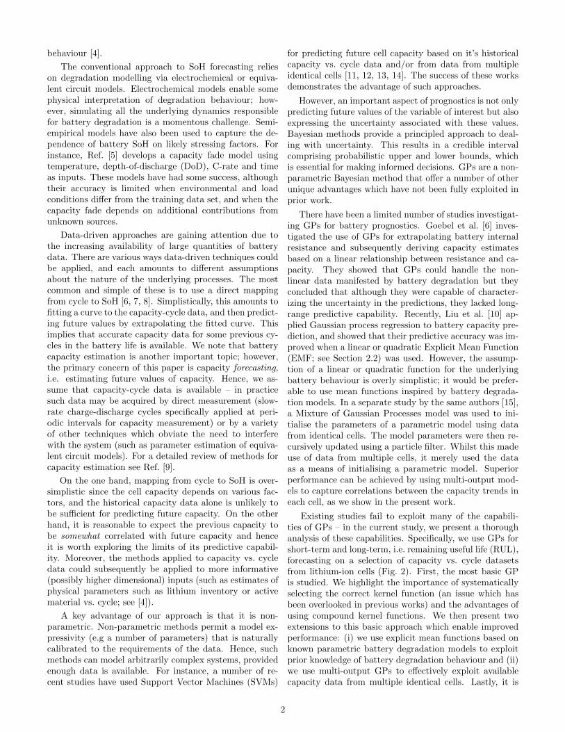
Figure 2: Battery datasets. a, NASA Battery Data Set used with the basic, single-output GP (Figs. 3 - 6), b, Dataextracted from Liu et al. [10] and used with the explicit mean function GP (Fig. 7) c, NASA Randomized Battery Usage DataSet used with the multi-output GP (Fig. 8). Note that the capacity is normalised against the starting capacity in each case.

worth underscoring the fact that all the methods presentedhere are rigorously evaluated using different proportions oftraining data (i.e. using capacity data up to the currentcycle for training, with various different values of the cur-rent cycle). This is in contrast to most previous studies onbattery prognostics, which merely evaluate the accuracy ofthe predictions made at a single arbitrarily selected cycle(e.g. the first half of training data).

2 Methods

The goal of a regression problem is to learn the map-ping from inputs x to outputs y, given a labelled train-ing set of input-output pairs D = {(xi, yi)}ND

i=1, where NDis the number of training examples. In our case, the in-put xi ∈ Z+ is the integer number of cycles applied upto the current cycle, and the output yi ∈ R+ is the corre-sponding measured capacity (all capacities are normalisedagainst the initial, maximum capacity). We assume theunderlying model takes the form y = f(x) +ε, where f(x)represents a latent function and ε ∼ N (0, σ2) is an inde-pendent and identically distributed noise contribution.

The learned model can then be used to make predic-tions at test indices x∗ = {x∗i }

NTi=1 (cycles at which we

wish to estimate the capacity) for unknown observationsy∗ = {y∗i }

NTi=1, where NT is the number of test indices.

In our case we are interested in extrapolation to forecastfuture values of capacity (and so the test indices are thefuture cycles up until the end of life (EoL)). The EoLis reached when the capacity drops below a predefinedthreshold denoted by yEoL; the corresponding cycle num-ber at which this occurs is denoted xEoL. Note that xEoL

is a-priori unknown, we will infer it using our model.We evaluate our methods using two different metrics,

which reflect the quantities of interest in a practical appli-cation: the first is the root-mean-squared error (RMSE)in the capacity estimation, which we denote RMSEQ. Ata given cycle, c, where we train using data up to the cur-rent cycle (x = [1, 2, . . . c]T ) and test on the remainder(x∗ = [c+1, c+2, . . . xEoL]T ), RMSEQ is defined as

RMSEQ(yi∗, y∗i ) =

√√√√ 1

NT

NT∑i=1

(yi∗ − y∗i )

2(1)

where yi is the estimate given data only up to and includ-ing c. By taking only one training proportion (i.e. a singlevalue of c), we would obtain just a single RMSEQ value.This would run the risk of misrepresenting the true perfor-mance of the method over the full cycle-life. For instance,it would not be acceptable for the estimates to be accurateafter the first 30 cycles are observed but to then divergewhen the next 5 cycles are received. Hence, in order tothoroughly validate our methods, we test the performanceusing all values of c from 20% of the cycle-life onwards.We thus obtain a value of RMSEQ at each cycle, and canplot RMSEQ vs. cycle (see later). This is in contrast tomost previous studies, which use just a single arbitraryvalue of c.

The second metric is the RMSE in the EoL prediction,which we denote RMSEEoL. For each value of c, thereis a single EoL prediction. Hence, we can compare thepredictions at all c values against the true EoL to obtaina mean error, defined as

RMSEEoL(x∗EoL, j , x∗EoL) =

√√√√ 1

Nc

Nc∑j=1

(x∗EoL, j − x∗EoL

)2(2)

where xEoL is the estimate given data only up to and in-cluding c, and Nc is the number of cycles at which we test(i.e. the number of different values of c).

Note that this metric neglects the intermediate valuesof the capacity between the current cycle and the EoL.For instance, two cells could have very different capacitytrajectories over the duration of their lives, whilst stillreaching their EoL after a similar number of cycles. Hence,a good model should have low values of both of the abovemetrics.

2.1 Gaussian process regression

This section gives an overview of Gaussian process regres-sion. For simplicity, our presentation assumes the inputsand outputs are scalar, since we only consider 1-D capac-ity vs. cycle data in this work. However, the analysis caneasily be extended to multidimensional inputs, if desired.A more detailed presentation of Gaussian process regres-sion (GPR) is given in Chapter 15 of [16], and a morecomprehensive book on the topic is [17].

3

A Gaussian process (GP) defines a probability distribu-tion over functions, and is denoted as:

f(x) ∼ GP(m(x), κ(x, x′)

), (3)

where m(x) and κ(x, x′) are the mean and covariance func-tions respectively, denoted by

m(x) = E[f(x)], (4)

κ(x, x′) = E[(f(x)−m(x)) (f(x′)−m(x′))T

]. (5)

For any finite collection of input points, say x =x1, ..., xND

, this process defines a probability distributionp (f(x1), ..., f(xND

)) that is jointly Gaussian, with somemean m(x) and covariance K(x) given by Kij = κ(xi, xj).

Gaussian process regression is a way to undertake non-parametric regression with Gaussian processes. The keyidea is that, rather than postulating a parametric form forthe function f(x, θ) and estimating the parameters θ (as inparametric regression), we instead assume that the func-tion f(x) is a sample from a Gaussian process as definedabove.

The most common choice of covariance function is thesquared exponential (SE), defined by

κSE(x, x′) = θ2f exp

(− 1

θ2l‖x− x′‖2

). (6)

The covariance function parameters1, θf and θl, controlthe y-scaling and x-scaling, respectively.

The SE kernel is a stationary kernel, since the correla-tion between points is purely a function of the differencein their inputs, x − x′. We only consider stationary ker-nels in this work. The choice of the SE kernel makes theassumption that the function is very smooth (infinitely dif-ferentiable). This may be too strict a condition for manyphysical phenomena [18], and so a common alternative isthe Matern covariance class:

κMa(x− x′) =

σ2 21−ν

Γ(ν)

(√2ν

(x− x′)ρ

)νRν(√

2ν(x− x′)

ρ

), (7)

where ν is a smoothness hyperparameter (larger ν impliessmoother functions) and Rν is the modified Bessel func-tion. This equation simplifies considerably for half-integerν. The most common examples are ν = 5/2 and ν = 3/2,which we denote as Ma5 and Ma3 in this work. The fi-nal covariance we consider in this paper is the periodiccovariance,

κPe(x, x′) = θ2f exp

(− 2

θ2lsin2

(πx− x′

p

))(8)

which is suitable for functions with periodic behaviour.The hyperparameter p is the period of f(x).

1The term ‘non-parametric’ is evidently a misnomer since thecovariance function contains parameters; however, these are techni-cally hyperparameters [17] since they are the parameters of a priorfunction.

Compound kernels can be created by affine transforma-tions of individual kernels. We limit our attention in thispaper to addition of kernels, since these were found tobe capable of expressing the structure of the battery dataunder study, and since they lead to greater ease of inter-pretation than multiplicative kernels. Ref. [19] providesa more detailed discussion of kernel composition and alsoaddresses the issue of automating the choice of kernels.In summing kernels, the data are modelled as a superpo-sition of independent functions. This can be interpretedas different processes operating at different input and/oroutput scales.

The mean function is commonly defined as m(x) = 0since the GP is flexible enough to model the true mean ar-bitrarily well. In Section 2.2, we consider parametric mod-els (based on battery degradation models) for the meanfunction, such that the GP models only the residual er-rors.

Now, if we observe a labelled training set of input-output pairs D = {(xi, yi)}ND

i=1, predictions can be made attest indices x∗ by computing the conditional distributionp(y∗|x∗,x,y). This can be obtained analytically by thestandard rules for conditioning Gaussians [16], and (as-suming a zero mean for notational simplicity) results in aGaussian distribution given by:

p(y∗|x∗,x,y) = N (y∗|m∗,Σ∗) (9)

where

m∗ = K(x,x∗)TK(x,x∗)−1y (10)

Σ∗ = K(x∗,x∗)−K(x,x∗)TK(x,x∗)−1K(x,x∗). (11)

The values of the hyperparameters θ may be optimisedby minimising the negative log marginal likelihood de-fined as NLML = − log p(y|x, θ). The NLML automat-ically performs a trade-off between bias and variance, andhence avoids over-fitting the data. Given an expressionfor the NLML and its derivative w.r.t θ (both of whichcan be obtained in closed form), we can estimate θ usingany standard gradient-based optimizer. In our case, weused the GPML toolbox [20] implementation of conjugategradients. Since the objective is not convex, local min-ima can be a problem. However, this was not an issue inthe present study, as was verified by repeated diverse ini-tialisations using Latin hypercube sampling [21] yieldingidentical results. Minimising the NLML further allows usto perform model selection, i.e. to choose the kernel func-tion, not just the values of the hyperparameters for a givenkernel function. Kernel function selection is perhaps themost important aspect of GP modelling, yet it has notbeen addressed in a principled manner in the aforemen-tioned battery degradation literature [6, 10, 15]

2.2 Explicit mean functions

Explicit mean functions (EMFs), also referred to as ex-plicit basis functions [17] or semi-parametric Gaussian pro-cesses [16], allow us to express prior information we may

4

have about the expected functional form of the model. Forinstance, let’s say we have a battery degradation modelwhich predicts capacity fade of the form y = m(x; θdeg)where θdeg are the parameters of the degradation model,but we believe that there may be other contributions tothe battery capacity fade that the model does not accountfor. We can then model the capacity as the sum of a GPand the parametric model:

y = m(x, θdeg) + f(x, θ) + ε (12)

This formulation expresses that the data are close to thedegradation model with the residuals being modelled by aGP (and a noise term). When fitting this model, we opti-mize over the degradation model parameters θdeg jointlywith the hyperparameters θ of the covariance function.

2.3 Multi-output GPs

If we have capacity vs. cycle data for multiple batteriesundergoing similar loading profiles, we may expect the ca-pacity trends to be correlated. This prior assumption canbe modelled using multi-output GPs. This section drawslargely from previous works on multi-output GPs [22, 23];and further details of similar methods can be found inthose works.

A function with multiple outputs can be dealt with bytreating it as having a single output and an additionalinput. This additional (discrete) input, l, can be thoughtof as a label for the associated output. Let’s say we havem cells whose inputs and outputs are {xl,yl}ml=1, where

{xl,yl} = {(xi, yi)}Nli=1, and Nl is the number of training

points associated with cell l. Each input of the multi-output model is then a 1 × 2 vector defined as xi,l =[xl(i), l], and this has an associated scalar output yi,l =yl(i). Assuming, for notational simplicity, that all cells areobserved at the same set of cycles and hence Nl = n for alll, we can now write the entire set of inputs and outputsas X = {{xi,j}ni=1}

ml=1 and y = {{yi,j}ni=1}

ml=1. A new

covariance function can then be defined as the product ofa label covariance and a standard covariance

κMOGP(x, x′, l, l′) = κl(l, l′)× κx(x, x′) (13)

where κl captures the correlation between outputs, and κxis the covariance with respect to cycles for a given output.The covariance matrix for all n cells is then the mn×mnmatrix defined by

KMOGP(X,L, θl, θx) = Kl(l, θl)⊗Kx(X, θx) (14)

where ⊗ is the Kronecker product, L = {l}mj=1, and θl andθx are the hyperparameters for Kl and Kx respectively.Note that the assumption that Nl = n for all cells caneasily be relaxed such that the model may be applied toproblems with capacities observed at different cycles foreach cell.

Lastly, we parametrise the label covariance matrix usinga spherical parametrisation scheme [22]:

Kl = STSdiag(τ) (15)

where τ = {τl}ml=1 is a vector of output scales correspond-ing to the different values of l, and S is an upper triangularmatrix of size m×m, whose lth column contains the spher-ical coordinates in Rl of a point on the hypersphere Sl−1,followed by the requisite number of zeros. For example, Sfor a three dimensional space is

S =

1 cos(φ1) cos(φ1)0 sin(φ1) sin(φ2) cos(φ3)0 0 sin(φ2) sin(φ3)

(16)

Note that this ensures that STS has ones across its diago-nal and hence all other entries may be thought of as akinto correlation coefficients, lying between −1 and 1.

The full set of hyperparameters, θl, therefore consists ofthe values of φl and τl. If the output scales are expectedto be the same for each cell (as we assume in the presentwork), then the values of τl can be fixed to a single value, τ .In this case, the total number of hyperparameters requiredis 1

2 (m+ 1).Once a suitable covariance has been defined, parametri-

sation and test prediction can be achieved in the samemanner as that of single-output GPs, using optimisationof the NLML to select the hyperparameters of the jointcovariance matrix. The advantage of the multi-outputscheme is that similarities between cells can be captured(through the shared hyperparameters, θx), without im-posing strict equivalence (through the cell-specific differ-ences induced by the label hyperparameter, θl). We em-ploy a standard implementation of this method, whichscales as O(m3n3). However, we note various differentefficient/approximate schemes have been proposed in theliterature, based on approximating input data with pseudopoints [24], exploiting grid structure [25] and exploitingthe recursivity of the estimation problem in online set-tings [22, 26, 27]; and these could be used if larger numbersof cells/training points were required.

3 Basic single-output GP – Re-sults

The first example we consider is a basic single-output GPwith a constant prior mean set equal to the mean of theobserved capacity data. The dataset considered consistsof capacity vs. cycle data obtained from the NASA batterydata repository (see Appendix A, and Fig. 2a). Here, wepresent the results for Cell A1, although similar resultswere obtained for Cells A2-A4.

3.1 Kernel function selection

It is apparent from Fig. 2a that the capacities experiencea long-term downward trend with occasional, apparentlydiscontinuous, step increases. In other words, they ex-hibit a combination of short- and long- term structure.The physical explanation for the short term jumps is notclear – it may in fact be an artefact of the measurement

5

process. For instance, the data indicates that these in-creases tend to occur after long periods without cycling,possibly when reference tests were performed, which indi-cates that the capacity increase may be related to thesepauses. In any case, accounting for these local variationsby means of appropriate kernel function selection is essen-tial since: (i) the capacity measurement provided in a realapplication could also manifest similar artefactual varia-tions, and (ii) accounting for such artefacts is necessary inorder to correctly express the uncertainty in subsequentmeasurements obtained via the same process.

In order to identify a suitable compound kernel func-tion, we assessed 10 different compound kernels: namely,all possible pairs of the following base kernels: Matern5/2 (Ma5), Matern 3/2 (Ma3), Squared Exponential (SE)and Periodic (Pe). The NLML of the GP when appliedto the full capacity vs. cycle data was used to evaluatethe kernel combinations. The ranking of these results isshown in the bar-plot of Fig. 3. This plot shows that fourcombinations achieve an NLML between 527 and 530, andhence perform similarly well. The performance then dropsoff more rapidly for the subsequent 5 combinations, andfinally the last combination (Pe+Pe, NLML = 97.1) per-forms significantly worse than the others. This is perhapsnot surprising given the lack of any exactly periodic struc-ture in the data, let alone a superposition of two periodiccomponents.

Ma3+Ma3

Ma3+Ma5

Ma5+Ma5

Ma5+SESE+SE

Ma3+SE

Pe+Ma3Pe+SE

Pe+Ma5Pe+Pe

0

200

400

600

Neg

. log

mar

gina

l lik

elih

ood

530 529 528 527 521 521 506 500 485

97.1

Figure 3: Ranking of kernel function combinations bymarginal likelihood. The coloured bars for selected kernelpairs correspond to the coloured lines in Figs. 4a and 4b.

Although Ma3+Ma3 was the highest ranked pair, itperformed only marginally better than the second rankedpair, Ma5+Ma3 (red bar in Fig. 3). Hence we chose thelatter for subsequent analysis because the contributions ofeach base kernel are easily interpretable.

3.2 Kernel function decomposition

In order to highlight the significance of kernel functionselection, the posterior mean and covariance for selectedkernel pairs are decomposed into their constituent con-tributions in Fig. 4 (using equations 2.17 and 2.18 from[28]).

Fig. 4a shows the decomposition of the selectedMa5+Ma3 kernel pair, evaluated using 55% of the cycle-

capacity data and tested on the remainder. The sub-plotsbeneath each main plot show the individual contributions,including the noise covariance (which is implicitly includedin each model). It can be seen that the Ma5 term capturesthe smooth long-term downward trend as desired, with anincreasing uncertainty as it is projected into the future;the Ma3 term captures the short term variation; and thenoise term models the remaining small scale variation inthe data. As a result, the extrapolation performance atthis particular cycle is quite good, as indicated by theclose match between the mean prediction and the truedata for the remaining cycles. Fig. 4b shows the resultfor a kernel pair which performed less well (NLML = 500,Fig. 3). In this case, the long-term trend is captured bythe periodic component, whilst the Ma5 term is forced tomodel the short term variation. This indicates that thereis little actual periodic structure present in the data, sincethe optimised length-scale of the periodic term is similarto the time-scale of the data, and hence only half a cycleof the periodic term is modelled. The predictions fromthis model indicate that the capacity will increase in thesubsequent 100 cycles, before decreasing again and thenrepeating this behaviour periodically, which is clearly un-realistic. Finally, Fig. 4c shows the decomposition of asingleton SE kernel function (i.e. not the sum of two basekernels). In this case, the SE term is forced to try to modelboth the long and short term trends in the data. This re-sults in the long-term trends being heavily influenced bythe short term variations. Hence, when the short termstep increase at ∼ cycle 90 is reached, the model predictsa smooth increase (then subsequent decrease) in the gra-dient, which is unrepresentative of the data. Moreover,there is obvious structure still present in the noise contri-bution (bottom sub-plot), which indicates that not all ofthe structure in the data has been captured by the model.Both of these attributes are clearly undesirable and leadto poor extrapolation performance.

3.3 Short-term lookahead prediction

Having selected a suitable kernel function, we now investi-gate the extrapolation performance using training data upto various different current cycles, c. Fig. 5 shows the per-formance of the method for n-step lookahead forecasting.Fig. 5a shows the posterior mean and covariance usingprediction horizons of 5, 10, 20 and 40 cycles. For eachcycle number, the posterior is obtained using data up tothe current cycle, and the mean and standard deviationare evaluated at the cycle n steps ahead of the currentcycle. This is repeated at every cycle up until the verticaldashed line (equal to the number of the last cycle minusthe size of the prediction horizon). Hence, the posteriormean and variance shown in the plots is the amalgamatedposterior from all of these cycles.

The plots show that the method is highly accurate forrelatively small n but that the performance diminishes asn is increased. This is hardly surprising given that wehave no a-priori reason to believe that the capacity data

6

0.6

0.8

1Capacity

Ma5+Ma3

0.5

1

Ma5

-0.04-0.02

00.020.04

MMa3

0 50 100 150

Cycles

-0.010

0.01

Noise

0.6

0.8

1

Capacity

Ma5+Pe

0.60.81

Per

-0.020

0.02

Ma5

0 50 100 150

Cycles

-0.02-0.01

00.01

Noise

0.6

0.8

1

Capacity

SE

00.51

SE

0 50 100 150

Cycles

-0.020

0.02

Noise

Ma5+Ma3 SE+Per SE

a b c

Figure 4: Decomposition of posterior functions into constituent kernels. The top plot in each column shows theposterior mean and credibility interval of the compound kernel. For this and all subsequent figures, the black markers indicatedata-points used for training, and the continuous black line indicates testing data, the coloured line indicates the mean of theposterior, and the correspondingly coloured shaded region indicates the area enclosed by the mean plus or minus two standarddeviations. The vertical line indicates the extent of the training data. a, Ma5+Ma3 (the selected kernel pair); b, SE+Per (apoorly performing kernel pair); c, SE (a singleton kernel)

up to a given cycle has strong predictive capabilities fordistant future cycles.

However, it is clear that the principled selection of thekernel function has been advantageous, since the methodclearly outperforms the singleton Ma5 GP. Fig. 5b showsbox-plots of the extrapolation error for various predictionhorizons for the Ma5-Ma3 GP, whilst Fig. 5c shows thesame data for the singleton Ma5 GP. Lastly, we evaluateda more conventional time-series approach, an autoregres-sive moving average of order 10 (i.e. using the 10 most re-cent data-points for training at each cycle), which is shownin Fig. 5c.

The Ma5+Ma3 GP has the best performance of thesethree, as shown by Fig. 5e which plots the RMSE againstprediction horizon of each of the three cases on a singleaxis for ease of comparison. This can be attributed to thefact that the additive kernels are capable of handling theprocesses of different scales – with the short term variationbeing handled by one of the constituent kernels and thelong-term downward trend by the other.

3.4 Remaining useful life prediction

Depending on the requirements of the system, predictingfuture capacity 10 cycles ahead with reasonable accuracymay be sufficient to facilitate corrective action. In somecases, however, it may be desirable to accurately estimatethe remaining useful life (RUL) from the earliest stagepossible, in which case accurate long-term prediction isimportant.

Fig. 6 shows the performance of the method for esti-mating the end of life (EoL) at three different current cyclevalues. The method shows some desirable properties, suchas converging to the correct EoL estimate as more train-

ing data are acquired and having large credible intervalswhen the extrapolation is far into the future. It also out-performs the baseline autoregressive model. However, theEoL predictions are poor at the initial cycles when thereare limited training data available. For instance, it canbe seen from Fig. 6a-b that the EoL is first severely over-estimated and then severely underestimated as new dataare received. This results in only moderate overall perfor-mance as indicated by the corresponding RMSEEoL values(see inset of Fig. 6d. This plot also shows the credibilityintervals in the EoL estimate. These were obtained by ex-trapolating the upper and lower confidence intervals in thecapacity estimates until they reached the EoL value. Insome cases the upper confidence interval never crosses thelower threshold and hence the upper EoL estimate is verylarge or infinite (extending beyond the upper limit of they-axis in this plot). This is an unfortunate consequence ofthe fact that the model is not restricted to be monotonic,as we discuss in Section 6. However, it is promising thatfrom about a third of the training data onwards, the trueEoL estimate always remains within the lower confidenceinterval.

4 Encoding exponential degrada-tion via EMFs – Results

In order to improve the long term predictive forecasts, wenow consider a single-output GP with an explicit meanfunction based on a battery degradation model from theliterature. The dataset in this case consists of capacityvs. cycle data extracted from [13] (see Appendix A, andFig. 2b). Here, we apply the method to Cell B3 sincethis exhibits the greatest deviation from the exact expo-

7

5 10 15 20 25 30 35

Predictionyhorizon

0.02

0.04

0.060.08

RM

SE

Ma5+Ma3

MA5AR

2y 6y 10 14 18 22 26 30 34 38

Predictionyhorizon

0

0.02

0.04

0.06

0.08

Abs

yerr

or

yMa5+Ma3

2y 6y 10 14 18 22 26 30 34 38

Predictionyhorizon

0

0.05

0.1

0.15

Abs

yerr

or

yMa5

2y 6y 10 14 18 22 26 30 34 38

Predictionyhorizon

0

0.1

0.2

0.3

0.4

Abs

yerr

or

yARb

0 50 100 150

Cycles

0.6

0.7

0.8

0.9

1C

apac

ity

ny=y5

a

c

d

e

0 50 100 150

Cycles

0.6

0.7

0.8

0.9

1

Cap

acity

ny=y10

0 50 100 150

Cycles

0.6

0.7

0.8

0.9

1

Cap

acity

ny=y20

0 50 100 150

Cycles

0.6

0.7

0.8

0.9

1

Cap

acity

ny=y40

Figure 5: Short term lookahead prediction performance. a, Posterior distribution of the Ma5+Ma3 GP for a range ofdifferent prediction horizons as indicated. b-d, Box-plot of capacity prediction errors for b, the Ma5+Ma3 GP, c, the singletonMa5 GP and d, an autoregressive moving average of order 10. e, RMSEQ of each method plotted on the same axis with they-axis in log scale for ease of comparison.

nential decay behaviour of the model, and hence bene-fits most from the additional non-parametric contributionsprovided by the GP.

We use an explicit mean function of the form m(x) =a1 + a2 exp (a3 x). The model parameters are thus givenby θdeg = [a1, a2, a3]. This function is equivalent to thedegradation model used by Goebel et. al [6]. It could alsobe viewed as a special case of the three-parameter degra-dation model used by Wang et al. [13] with the “empiricalfactor” set to zero (i.e. g = 0 in Eq. (21) of [13]).

We consider three different GP models:

a. y = f(x) +m(x), where f(x) ∼ GP (0, κMa3)

b. y = f(x) +m(x), where f(x) = ε ∼ GP (0, κnoise)

c. y ∼ GP (0, κMa5+Ma3)

Model (a) assumes that the response consists of thespecified exponential mean function plus a GP with Ma3covariance. Model (b) is identical to (a) but with a noisecovariance; since the covariance is simply white noise, thisis essentially just a parametric model. Model (c) is the ba-sic GP that gave best results in the previous section (i.e.with a zero mean function but with a covariance functionconsisting of a sum of Ma5 and Ma3 terms).

Fig. 7 shows the posterior predictions at two arbitrarilychosen cycles (top) and the estimated EoL (bottom) foreach of the three cases.

It can be seen from this figure that model (c) performspoorly in the region of ∼60 cycles, where the capacitytemporarily levels off. This is because the model hasno prior assumption encoded about the degradation be-haviour (other than the smoothness assumptions encodedby the covariance) and hence, when only the data up untilthis time step are used for training, it predicts a subse-quent upwards trend in the capacity. This can be seenfrom the bottom plot of Fig. 7c in the same region, whichshows that the EoL prediction extends beyond the upperlimit of the y-axis. In contrast, models (a) and (b) copewith this temporary stationary behaviour and correctlypredict a continuing exponential degradation for subse-quent time steps. As a result of this, models (a) and (b)also have lower overall RMSEEoL values than model (c).Hence, these results show that the use of an explicit meanfunction improves the overall accuracy of the EoL predic-tions.

Comparing model (a) against model (b), we can see theadvantage of using a GP model over a purely paramet-ric model. Since model (b) assumes that any deviation

8

0 50 100 150 200

Cycles

0.6

0.7

0.8

0.9

1C

apac

ityMa5+Ma3g(cycleg50)g

0 50 100 150 200

Cycles

0.6

0.7

0.8

0.9

1

Cap

acity

Ma5+Ma3g(cycleg81)g

0 50 100 150 200

Cycles

0.6

0.7

0.8

0.9

1

Cap

acity

Ma5+Ma3g(cycleg141)g

0.4 0.6 0.8

Proportiongofgtraininggdata

0

100

200

300

EoL

g(cy

cles

)

Ma5+Ma3g(RMSEEoL:g56.1)ARg(RMSEEoL:g96.2)

a b c d

Figure 6: End of life (EoL) estimation performance. a-c, Posterior distribution of the Ma5+Ma3 GP at 3 differentproportions of the training data. The horizontal black line indicates the capacity at the EoL. d, Predicted cycle no. at EoLvs. training data proportion for the GP and AR methods. The shaded region indicates the confidence interval in the EoLprediction. Note that there is no green shaded area since the AR does not provide confidence bounds. The horizontal blackline indicates the true EoL.

0 50 100 150 200

Cycles

0.7

0.8

0.9

1

Cap

acity

EMFf+fMA3f

0.2 0.4 0.6 0.8

Proportionfofftrainingfdata

0

100

200

EoL

f:cy

cles

N

RMSEEoL:f47.1fcycles

0 50 100 150 200

Cycles

0.7

0.8

0.9

1

Cap

acity

EMFf+fNoisef

0.2 0.4 0.6 0.8

Proportionfofftrainingfdata

0

100

200

EoL

f:cy

cles

N

RMSEEoL:f50.2fcycles

0 50 100 150 200

Cycles

0.7

0.8

0.9

1

Cap

acity

MA5+MA3f

0.2 0.4 0.6 0.8

Proportionfofftrainingfdata

0

100

200

EoL

f:cy

cles

N

RMSEEoL:f76.5fcycles

a b c

Figure 7: Explicit mean function GP results. a-c, (top) Posterior distribution at 2 different proportions of the trainingdata for a, EMF+Ma3, b, EMF+Noise and c, Ma5+Ma3. The horizontal black line indicates the capacity at the EoL. (bottom)Predicted cycle no. at EoL vs. training data proportion for the corresponding methods. The shaded region indicates the credibleinterval in the EoL prediction. The horizontal black line indicates the true EoL cycle.

from the exponential model must be noise (since the ker-nel function is defined to be white noise), the optimisednoise parameter becomes quite large and the credible in-terval increases to encompass the spread in observed ca-pacities. In contrast, model (a) models the deviations withan Ma3 kernel, and hence can fit the non-exponential trendquite well, whilst maintaining a sensible assumption forthe noise levels.

Lastly, it should be noted that models (a) and (b) areboth overconfident in their predictions (the credibility in-tervals in the EoL estimation in the bottom plots are toonarrow and do not encompass the true EoL for most of thetraining proportions). Moreover, in some cases the uncer-tainty is seen to decrease with increasing cycle number, inparticular in model (b). This is obviously not desirablebehaviour and is an indication that the assumption of thefunctional form of the underlying model (i.e. the expo-nential degradation model) is not entirely valid for this

data.

5 Capturing cell-to-cell correla-tions via multi-output GPs –Results

The final example we consider is a multi-output GP. Thedataset in this case consists of capacity vs. time datafrom three cells with randomised load profiles (see A, andFig. 2c). Since the cell cycling is randomised, a parametricdegradation model (which is a function of the number ofcycles) would be unsuitable. Hence, we rely on exploitingdata from existing cells to improve the long-term forecast.We apply the method to cell C3 using data from cells C1and/or C2 for training as follows.

We considered four different models:

9

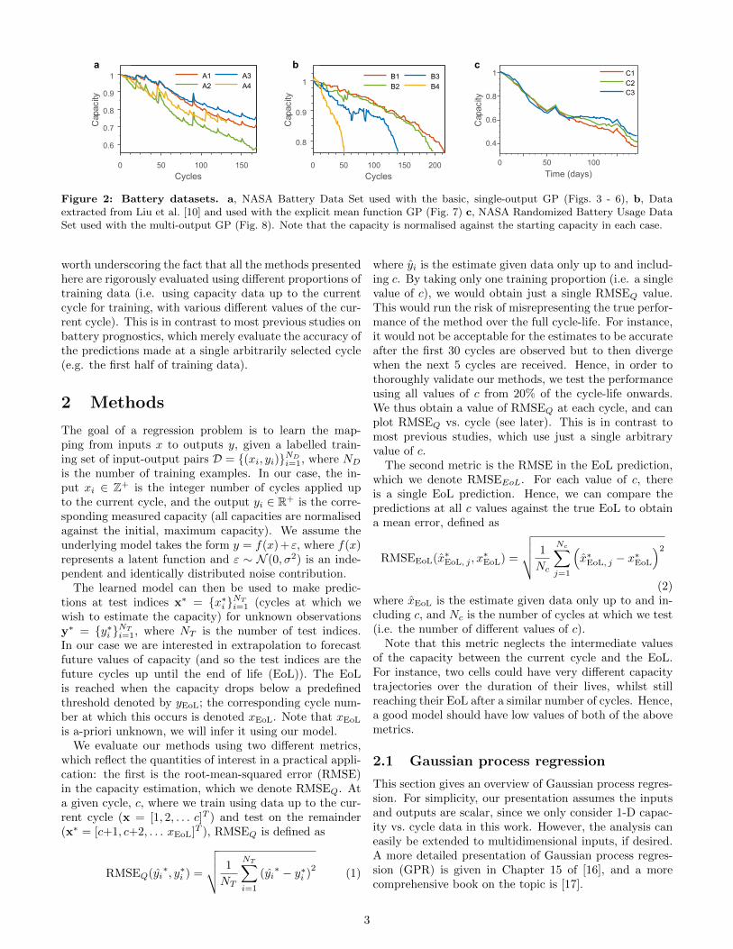
a. A multi-output GP with 3-outputs: the capacity datafor cells C1-C3. The model is trained on all capacitydata for cells C1 and C2, along with data up until thecurrent cycle for cell C3, in the same manner as theprevious test cases.

b. A multi-output GP with 2-outputs: the capacity datafor cells C1 and C3 (omitting C2). The model istrained on all of the capacity data for cell C1, alongwith data up until the current cycle for cell C3 asbefore.

c. A multi-output GP with 2-outputs as in (b) but pro-vided with data from C2 instead of C1.

d. A standard single-output GP trained using just dataup to the current cycle for C3.

The multi-output models were defined as described inSection 2.3, with the κMOGP = κl × κx where κl is thelabel covariance matrix (Eq. 15), and κx = κMa5+Ma3.The covariance of the single output model was simply κ =κx = κMa5+Ma3.

The training data and results for these four cases areshown in Fig. 8. Figs. 8a-d show the data used for trainingat a selected time step (top), the posterior predictions atthe corresponding time step (middle), and the estimatedEoL as a function of the number of cycles of cell C3 train-ing data used (bottom) for each of the four cases. Figs. 8e-g show summary statistics for all four cases: Fig. 8e showsRMSEQ as a function of the proportion of the trainingdata (for cell C3) used. Fig. 8f shows a boxplot of thesame data. Fig. 8g shows a bar plot of RMSEEoL.

It can be seen from these results that the multi-outputmodels (a-c) have better predictive performance than thesingle output model (d). For instance, in the middle sub-plots in Fig. 8a-d (which show the posterior prediction at75 days), all of the multi-output models accurately trackthe future capacity up until the predicted EoL, whereasthe single output method does not anticipate the suddendrop in capacity at ∼125 days, and hence over-predicts thesubsequent capacity. Indeed, the estimates of the EoL ofcell C3 are quite accurate throughout the entire range oftraining data (bottom subplots) for the multi-ouput meth-ods, but are shown to fluctuate significantly as additionaltraining data are received in the single-output case. Thisis also reflected in the overall RMSEQ and RMSEEoL val-ues depicted in Figs. 8e-g.

Interestingly, there are significant differences in the per-formance of models b and c (which are both two out-put models); for instance, model b, which is trained oncell C1, has an RMSEEoL of 18.1, whereas model c, whichis trained on cell C2, has an RMSEEoL of 4.86. Likewise,there is greater uncertainty (larger error bounds) in theposterior predictions of model b than those of model c (seee.g. middle subplots of Fig.8b and c). This indicates thatthe capacity trend of cell C3 shares a stronger correlationwith that of cell C2 than that of cell C1.

It is perhaps even more interesting to note that model a(which has 3-outputs) is not negatively affected by theinclusion of data from Cell 1. Rather, the model naturallyputs more weight on the data from cell C2 (than fromcell C1) since this shows a stronger correlation with cellC3. As a result, the performance of model a turns outto be superior to either model b or model c in this case(Figs. 8f-g).

There are a number of obvious caveats to be aware of inthe present case: the method has performed particularlywell here because the dataset consists of cells cycled underthe same thermal conditions with statistically equivalentapplied current profiles2. Hence, there were strong corre-lations between the data for these cells. Whilst this couldoccur in practice in some limited cases (for instance, mul-tiple cells in a pack could experience the same conditions),in most cases of interest we would wish to use data fromidentical cells but cycled under differing conditions. Themethod could of course be extended to account for suchdifferences by including additional inputs, such as temper-ature or depth of discharge, although this would requiredata from many more cells to cover a broad range of oper-ating conditions. For such (larger) datasets, more efficientimplementation methods must be used, such as those dis-cussed in Section 2.3.

However, the present results indicate that the multi-output method has promise. In particular, it is favourableover previous GP capacity estimation methods that usedata from identical cells, which merely identify an optimalprior estimate for the parameters of a parametric model,which are then updated sequentially [10]. In such a settingthe advantage of the prior information is quickly lost. Incontrast, the present method exploits correlations in cellbehaviour over the duration of the cell life, which leads tothe improved results obtained here.

6 Conclusions

This paper has demonstrated the applicability of GPs tobattery capacity forecasting, and highlighted some of theirkey advantages for this application. We have shown theadvantage of using compound kernel functions for captur-ing complex behaviour and highlighted the importance ofproper kernel function selection by means of optimisingw.r.t. the NLML. We have shown that using an explicitmean function based on known degradation models, it ispossible to improve the predictive performance of the base-line GP. Indeed, we argue that one should never just con-sider a purely data-driven approach if prior informationon the functional form of the underlying model is avail-able; or a purely parametric approach if the model infor-mation is not known with certainty, since in either case

2Note that the applied current profiles are generated by a stochas-tic algorithm [29] and hence they are not identical from cell to cell.However, since the algorithm is the same for each cell, the globalproperties of these current profiles are the same, and so they mani-fest similar degradation behaviour.

10

0 100 200

TimeE(days)

0.2

0.4

0.6

0.8

1

Cap

acity

3-output

0 100 200

TimeE(days)

0.2

0.4

0.6

0.8

1

Cap

acity

0 100 200

TimeE(days)

0.2

0.4

0.6

0.8

1

Cap

acity

0 100 200

TimeE(days)

0.2

0.4

0.6

0.8

1

Cap

acity

1-output

050

100TimeE(days) 1 2 3

Cell

0

0.5

1

Cyc

les

0

0.5

0

Cyc

les

1

50

TimeE(days)3100

Cell

21

0

0.5

0

Cyc

les

1

50

TimeE(days)3100

Cell

21

0

0.5

0

Cyc

les

1

50

TimeE(days)3100

Cell

21

3-output

2-outputE

2-outputE1-output

0

0.05

0.1

0.15

0.2

0.25

RM

SE

0.2 0.4 0.6 0.8

ProportionEofEtrainingEdata

10-2

10-1

100

RM

SE

3-output2-output2-output1-output

0.2 0.4 0.6 0.8

ProportionEofEtrainingEdata

0

100

200

300

Pre

dict

edEE

oLE(

days

)

0.2 0.4 0.6 0.8

ProportionEofEtrainingEdata

0

100

200

300

Pre

dict

edEE

oLE(

days

)0.2 0.4 0.6 0.8

ProportionEofEtrainingEdata

0

100

200

300

Pre

dict

edEE

oLE(

days

)

1-output

3-output

2-output

2-output1-output

0

10

20

30

40

50

EoL

ERM

SE

E(da

ys)

4.57

18.1

4.86

46.2

0.2 0.4 0.6 0.8

ProportionEofEtrainingEdata

0

100

200

300

Pre

dict

edEE

oLE(

days

)

3-output

a b c d

e f g

2-outputE(i) 2-outputE(ii)

2-outputE(ii)2-outputE(i)

(i) (ii) (ii)(i)

(i)(ii)

Figure 8: Multi-output GP results. a-d, Data and results for a, 3-output, b, 2-output (i), c 2-output (ii), and d single-output GPs. (top) Battery data; black markers indicate training data and red line indicates unseen testing data. (middle)Posterior distribution using 40% of the training data and (bottom) Predicted cycle no. at EoL vs. training data proportion. e,RMSE vs. proportion of training data; f, Box-plot of RMSE data; and g, Bar plot of RMSE on EoL prediction. Note that thecolours of the lines/shaded regions in a-d correspond to the colours of the lines and bars in e and g.

one would be neglecting a valuable source of information.Lastly, we have shown that multi-output models can ef-fectively exploit data from multiple cells to significantlyimprove forecasting performance. The main bottleneck ofthis approach is the computational cost of handling largenumbers of outputs; although we applied this method toa small dataset of just 3 cells in the present case, efficientapproaches exist which allow scaling to very large numbersof outputs.

The present work aims to highlight just some of theadvantages of GPs. Several extensions/variations on thiswork are also possible. For instance:

• We know a-priori that the normalised cell capacitymust take a value between 0 and 1. In the present

work, this is not enforced and at times the GP maypredict values outside of this range (in particular forsingle-output GPs with limited training data). Oneway to enforce positive values is to apply a logit-transform to the data as a pre-processing step andapply a GP to the resulting data, then reverse trans-form the result.

• The notion that the future capacity depends onlyon the past values is naıve. A more comprehensivestudy could include DoD, temperature, idle time etc.as inputs. Whilst such dependencies have been con-sidered in a parametric framework in previous works(e.g. [5]), the application in a GP framework has notyet been considered, Such an approach would require

11

data from many more cells to cover a broad range ofoperating conditions.

• Cells often exhibit regime changes during aging (e.g.a transition from a linear capacity vs. cycle trendto a non-linear regime with accelerated aging [30]).GPs have the capability to account for such transi-tions; specifically, change-point kernels [31, 32] couldbe used to locate change points in an online manner,and hence more accurately model the regimes beforeand after a transition than would be possible with asingle model over the entire domain.

• The GP framework could also be applied using higherdimensional input data, such as open circuit voltagecurves or electrochemical impedance spectra acquiredat periodic cycles.

We hope that the present study has provided motiva-tion for further study of GPs applied to battery capacityforecasting.

A Data

The datasets (Fig. 1) consist of capacity vs. cycle data ob-tained from either open-access NASA repositories or ex-tracted directly from the plots in previous papers. In eachof these cases, the results obtained from a single selectedcell were presented in this paper; similar results were ob-tained for the other cells in each dataset, but for brevitythese were not presented.

Dataset A is obtained from the NASA Ames Prognos-tics Center of Excellence Battery Data Set[33]. The exper-iments consisted of applying several charge-discharge cy-cles to a number of commercially available 18650 lithium-ion cells at room temperature in order to achieve accel-erated aging. Charging was carried out via a constant-current, constant-voltage regime: charging at constantcurrent at 1.5 A until the voltage reached the cell uppervoltage limit of 4.2 V, then applying a constant voltageuntil the the current dropped to 20 mA. Discharging wascarried out at a constant current of 2 A until the cell volt-age fell to 2.7 V, 2.5 V, 2.2 V, and 2.5 V for batteries 5,6, 7, and 18, respectively. The experiments were stoppedwhen the batteries had lost 30% of the initial capacity.Additional data (including temperature and electrochem-ical impedance) are also provided in the online repository,although these were not used in the present study. Fulldetails of the experiments are available in Ref. [7].

Batteries 5, 6, 7, and 18 (in the numbering of the on-line repository) were chosen to be analysed in the presentwork, since these have the most data-points; and becausethey have previously been chosen for analysis in earlierworks [8, 10], and hence the present selection facilitatesa comparison with those works. For consistency, thesecells are labelled as A1, A2, A3 and A4 respectively inthe present paper (Fig. 2a). The results for Cell A1 arepresented in Section 3.

Dataset B was obtained by manually extracting thedata from the capacity vs. cycle plots in Fig. 1 of Ref. [8],using Matlab GRABIT (a tool for extracting raw datafrom plot images). These data were originally obtainedfrom charge-discharge experiments on a 0.9 Ah lithium-ion cell. The discharge rate was 0.45 A and the currentswere cut off at the upper and lower voltage limits specifiedby the battery manufacturer. Further details of the exper-iments are available in Ref. [8]. These cells are denotedB1, B2, B3 and B4 in the present paper (Fig. 2b). Theresults for Cell B3 are presented in Section 4.

Dataset C is obtained from the NASA Ames Prognos-tics Center of Excellence Randomized Battery Usage DataSet [29]. The experiments consisted of applying random-ized sequences of current loads ranging from 0.5 A to 4 Ato a number of LG Chem. 18650 lithium-ion cells at arange of environmentally controlled temperatures in orderto achieve accelerated aging. The sequence was random-ized in order to better represent practical battery usage.After every fifty randomized discharging cycles, the ca-pacity was measured via a low-rate charge-discharge cy-cle, and the electrochemical impedance were measured viaan EIS sweep. The experiments are described in detail inRef. [34].

The first three cells from Dataset 1, denoted RW9,RW10 and RW11 (in the numbering and labelling of theonline repository) were chosen for analysis. These cellswere cycled at room temperature and express highly non-linear and non-parametric behaviour. The cells are la-belled as C1, C2 and C3 in the present paper (Fig. 2c).The results for Cell C1 are presented in Section 5.

References

[1] E. Cabrera-Castillo, F. Niedermeier, A. Jossen, Cal-culation of the state of safety (sos) for lithium ionbatteries, Journal of Power Sources 324 (2016) 509–520.

[2] J. Neubauer, A. Pesaran, The ability of battery sec-ond use strategies to impact plug-in electric vehicleprices and serve utility energy storage applications,Journal of Power Sources 196 (23) (2011) 10351–10358.

[3] C. R. Birkl, D. F. Frost, A. M. Bizeray, R. R. Richard-son, D. A. Howey, Modular converter system for low-cost off-grid energy storage using second life li-ionbatteries, in: Global Humanitarian Technology Con-ference (GHTC), 2014 IEEE, IEEE, 2014, pp. 192–199.

[4] C. R. Birkl, M. R. Roberts, E. McTurk, P. G. Bruce,D. A. Howey, Degradation diagnostics for lithium ioncells, Journal of Power Sources 341 (2017) 373–386.

[5] J. Wang, P. Liu, J. Hicks-Garner, E. Sherman,S. Soukiazian, M. Verbrugge, H. Tataria, J. Musser,

12

P. Finamore, Cycle-life model for graphite-LiFePO 4cells, Journal of Power Sources 196 (8) (2011) 3942–3948.

[6] K. Goebel, B. Saha, A. Saxena, J. R. Celaya,J. P. Christophersen, Prognostics in battery healthmanagement, IEEE instrumentation & measurementmagazine 11 (4) (2008) 33.

[7] B. Saha, K. Goebel, Uncertainty management for di-agnostics and prognostics of batteries using Bayesiantechniques, in: Aerospace Conference, 2008 IEEE,IEEE, 2008, pp. 1–8.

[8] W. He, N. Williard, M. Osterman, M. Pecht, Prog-nostics of lithium-ion batteries based on Dempster–Shafer theory and the Bayesian Monte Carlo method,Journal of Power Sources 196 (23) (2011) 10314–10321.

[9] A. Farmann, W. Waag, A. Marongiu, D. U. Sauer,Critical review of on-board capacity estimation tech-niques for lithium-ion batteries in electric and hybridelectric vehicles, Journal of Power Sources 281 (2015)114–130.

[10] D. Liu, J. Pang, J. Zhou, Y. Peng, M. Pecht, Prognos-tics for state of health estimation of lithium-ion bat-teries based on combination Gaussian process func-tional regression, Microelectronics Reliability 53 (6)(2013) 832–839.

[11] X. Hu, J. Jiang, D. Cao, B. Egardt, Batteryhealth prognosis for electric vehicles using sample en-tropy and sparse Bayesian predictive modeling, IEEETransactions on Industrial Electronics 63 (4) (2016)2645–2656.

[12] M. A. Patil, P. Tagade, K. S. Hariharan, S. M. Ko-lake, T. Song, T. Yeo, S. Doo, A novel multistageSupport Vector Machine based approach for li ionbattery remaining useful life estimation, Applied En-ergy 159 (2015) 285–297.

[13] D. Wang, Q. Miao, M. Pecht, Prognostics of lithium-ion batteries based on relevance vectors and a condi-tional three-parameter capacity degradation model,Journal of Power Sources 239 (2013) 253–264.

[14] A. Nuhic, T. Terzimehic, T. Soczka-Guth, M. Buch-holz, K. Dietmayer, Health diagnosis and remaininguseful life prognostics of lithium-ion batteries usingdata-driven methods, Journal of Power Sources 239(2013) 680–688.

[15] F. Li, J. Xu, A new prognostics method for state ofhealth estimation of lithium-ion batteries based ona mixture of Gaussian process models and particlefilter, Microelectronics Reliability 55 (7) (2015) 1035–1045.

[16] K. P. Murphy, Machine learning: a probabilistic per-spective, MIT press, 2012.

[17] C. E. Rasmussen, Gaussian processes for machinelearning.

[18] M. L. Stein, Interpolation of spatial data: some the-ory for kriging, Springer Science & Business Media,2012.

[19] D. K. Duvenaud, J. R. Lloyd, R. B. Grosse, J. B.Tenenbaum, Z. Ghahramani, Structure discovery innonparametric regression through compositional ker-nel search., in: ICML (3), 2013, pp. 1166–1174.

[20] C. E. Rasmussen, H. Nickisch, Gaussian processesfor machine learning (GPML) toolbox, J. Mach.Learn. Res. 11 (2010) 3011–3015.URL http://dl.acm.org/citation.cfm?id=

1756006.1953029

[21] R. L. Iman, Latin hypercube sampling, Encyclopediaof Quantitative Risk Analysis and Assessment.

[22] M. Osborne, Bayesian Gaussian processes for sequen-tial prediction, optimisation and quadrature, OxfordUniversity New College, 2010.

[23] R. Durichen, M. A. Pimentel, L. Clifton,A. Schweikard, D. A. Clifton, Multitask Gaus-sian processes for multivariate physiological time-series analysis, IEEE Transactions on BiomedicalEngineering 62 (1) (2015) 314–322.

[24] M. A. Alvarez, N. D. Lawrence, Computationally ef-ficient convolved multiple output gaussian processes,Journal of Machine Learning Research 12 (May)(2011) 1459–1500.

[25] A. G. Wilson, H. Nickisch, Kernel interpolation forscalable structured Gaussian processes (KISS-GP),arXiv preprint arXiv:1503.01057.

[26] G. Pillonetto, F. Dinuzzo, G. De Nicolao, Bayesianonline multitask learning of gaussian processes, IEEETransactions on Pattern Analysis and Machine Intel-ligence 32 (2) (2010) 193–205.

[27] Y.-L. K. Samo, S. J. Roberts, p-markov Gaussianprocesses for scalable and expressive online Bayesiannonparametric time series forecasting, arXiv preprintarXiv:1510.02830.

[28] D. Duvenaud, Automatic model construction withGaussian processes, Ph.D. thesis, University of Cam-bridge (2014).

[29] B. Bole, C. Kulkarni, M. Daigle, Randomized bat-tery usage data set, NASA AMES prognostics datarepository.

13

[30] G.-w. You, S. Park, D. Oh, Diagnosis of electric ve-hicle batteries using recurrent neural networks, IEEETransactions on Industrial Electronics.

[31] Y. Saatci, R. D. Turner, C. E. Rasmussen, Gaussianprocess change point models, in: Proceedings of the27th International Conference on Machine Learning(ICML-10), 2010, pp. 927–934.

[32] R. Garnett, M. A. Osborne, S. Reece, A. Rogers, S. J.Roberts, Sequential Bayesian prediction in the pres-ence of changepoints and faults, The Computer Jour-nal 53 (9) (2010) 1430. doi:doi:10.1093/comjnl/

bxq003.

[33] B. Saha, K. Goebel, Battery data set, NASA AMESprognostics data repository.

[34] B. Bole, C. S. Kulkarni, M. Daigle, Adaptation ofan electrochemistry-based li-ion battery model to ac-count for deterioration observed under randomizeduse, in: Proceedings of Annual Conference of thePrognostics and Health Management Society, FortWorth, TX, USA, Vol. 29, 2014.

Acknowledgments

This work was funded by an RCUK Engineering and Phys-ical Sciences Research Council grant, ref. EP/K002252/1.

14