gems: An R Package for Simulating from Disease Progression Models Nello Blaser * University of Bern Luisa Salazar Vizcaya * University of Bern Janne Estill University of Bern Cindy Zahnd University of Bern Bindu Kalesan University of Bern Columbia University Matthias Egger University of Bern University of Cape Town Thomas Gsponer † University of Bern Olivia Keiser † University of Bern Abstract Mathematical models of disease progression predict disease outcomes and are useful epidemiological tools for planners and evaluators of health interventions. The R package gems is a tool that simulates disease progression in patients and predicts the effect of different interventions on patient outcome. Disease progression is represented by a series of events (e.g., diagnosis, treatment and death), displayed in a directed acyclic graph. The vertices correspond to disease states and the directed edges represent events. The package gems allows simulations based on a generalized multistate model that can be described by a directed acyclic graph with continuous transition-specific hazard functions. The user can specify an arbitrary hazard function and its parameters. The model includes parameter uncertainty, does not need to be a Markov model, and may take the history of previous events into account. Applications are not limited to the medical field and extend to other areas where multistate simulation is of interest. We provide a technical explanation of the multistate models used by gems, explain the functions of gems and their arguments, and show a sample application. This manuscript was published in the Journal of Statistical Software Blaser et al. (2015). Keywords : Monte Carlo simulation, multistate model, R, survival analysis, prediction, com- partmental model. 1. Introduction We present a simulation algorithm and the R package gems (Salazar Vizcaya et al. 2013) for simulating from a multistate model with arbitrary transition-specific hazard functions. In epidemiology, mathematical models of disease progression are useful for predicting disease * The first two authors listed on the paper contributed equally to the development of gems and to the writing of this manuscript. † The last two authors listed on the paper contributed equally to this manuscript.
Transcript
gems: An R Package for Simulating from Disease
Progression Models
Nello Blaser∗
University of BernLuisa Salazar Vizcaya∗
University of Bern
Janne EstillUniversity of Bern
Cindy ZahndUniversity of Bern
Bindu KalesanUniversity of Bern
Columbia University
Matthias EggerUniversity of Bern
University of Cape Town
Thomas Gsponer†
University of BernOlivia Keiser†
University of Bern
Abstract
Mathematical models of disease progression predict disease outcomes and are usefulepidemiological tools for planners and evaluators of health interventions. The R packagegems is a tool that simulates disease progression in patients and predicts the effect ofdifferent interventions on patient outcome. Disease progression is represented by a seriesof events (e.g., diagnosis, treatment and death), displayed in a directed acyclic graph. Thevertices correspond to disease states and the directed edges represent events. The packagegems allows simulations based on a generalized multistate model that can be described bya directed acyclic graph with continuous transition-specific hazard functions. The user canspecify an arbitrary hazard function and its parameters. The model includes parameteruncertainty, does not need to be a Markov model, and may take the history of previousevents into account. Applications are not limited to the medical field and extend to otherareas where multistate simulation is of interest. We provide a technical explanation of themultistate models used by gems, explain the functions of gems and their arguments, andshow a sample application. This manuscript was published in the Journal of StatisticalSoftware Blaser et al. (2015).
Keywords: Monte Carlo simulation, multistate model, R, survival analysis, prediction, com-partmental model.
1. Introduction
We present a simulation algorithm and the R package gems (Salazar Vizcaya et al. 2013) forsimulating from a multistate model with arbitrary transition-specific hazard functions.
In epidemiology, mathematical models of disease progression are useful for predicting disease
∗The first two authors listed on the paper contributed equally to the development of gems and to the writingof this manuscript.†The last two authors listed on the paper contributed equally to this manuscript.
2 Generalized Multistate Simulation Model
outcomes and for planning and evaluating interventions (Garnett et al. 2011). Disease pro-gression is often characterized by a series of events, such as diagnosis, treatment and death.From this characterization, disease progression can be displayed in a directed acyclic graph(DAG) (Pearl 2009), where disease states are denoted by vertices and the directed edgesconnecting them correspond to the events.
Traditional compartmental models of infectious diseases assume that transition times betweenthe different stages of a disease are exponentially distributed (Anderson and May 1992). Theuse of exponential transition times has the advantage that models can be formulated deter-ministically with ordinary differential equations. Exponential times can also be simulatedusing the Gillespie algorithm (Gillespie 1977). However, the distribution of transition timesbetween states is often not exponential (Lloyd 2001). Although it is possible to divide statesinto substates, so that an exponential transition-specific hazard fits the data for those sub-states, this approach is inflexible. Typical model structures using non-exponential transitiontimes are agent-based stochastic simulation models (Estill et al. 2012; Phillips et al. 2011).For instance one study used history-dependent Weibull distributed transition times to inves-tigate the effect on HIV transmission of bringing patients lost to follow-up back into care(Estill et al. 2014). This study found that 116 tracing efforts were needed to prevent onenew infection. Agent-based models usually apply to one specific disease and include a limitednumber of interventions. We are not aware of any agent-based model structure that can beapplied simultaneously to different diseases and interventions. We therefore propose a moreflexible simulation algorithm that can simulate from any DAG.
We developed a multistate model that allows disease progression to be monitored in a cohortof individual patients, and takes into account the history of previous events. The R packagegems allows simulation from a directed acyclic multistate model with general transition-specific hazard functions. The package simplifies definition of the multistate model, its rel-evant transition-specific functions, its parameters, and their uncertainty. It also calculatestransition probabilities and cumulative incidences, and thus facilitates analysis of the sim-ulated cohorts. The R package gems is used for simulation and not parameterization ofmultistate models. To parameterize the transition-specific hazard functions, the R packagessurvival (Therneau 2014), mstate (de Wreede et al. 2011) and muhaz (Hess and Gentleman2010) can be used.
In Section 2 we present a mathematical description of the multistate model. We presentthe simulation from this model and demonstrate the inclusion of parameter uncertainty. InSection 3, we describe the use of gems in detail, providing explanations for and examples of allthe important package functions. In Section 4 we present a case study in cardiology. Finally,in Section 5, we discuss the strengths and limitations of the package.
2. Technical description of the simulation model
We describe a directed acyclic multistate model and the algorithm used in gems to simulatefrom it. For a general introduction to multistate models, see Putter et al. (2007).
2.1. General setup of the multistate model
A multistate model consists of a set of states and the transitions between them. The statescan be divided into three groups: initial states, intermediate states and absorbing states.
Nello Blaser, Luisa Salazar Vizcaya, et al. 3
gems only considers multistate models without loops, that is models, which can be writtenas a directed acyclic graph (DAG) (Pearl 2009). A DAG consists of states and the directededges that connect them, so that no sequence of directed edges can connect back to a previousstate.
Consider a directed acyclic multistate model with n states E1, . . . , En, where a transitionfrom state Ei to state Ej is only possible if i < j. Let (Xt)t≥0 be the stochastic process thatdescribes the progression through the different states. It is an E = {E1, . . . , En}-valued jumpprocess with jump times given by
Si = inf {t ≥ 0 | Xt = Ei} (1)
for states Ei that are visited, and Si = ∞ otherwise. Transition times to state Ej from theprevious state are defined by Tj = Sj − Smax {k | k<j,Sk<∞}, where S0 = 0 by convention.
The entire process is determined by transition times Tj to state Ej , described by transition-specific hazard functions hij as
Tij ∼ Fij(t) = 1− exp
{−∫ t
0hij(u) du
}, (2)
Tj = mini∈{1,...j−1 | Ti<∞}
Tij , (3)
where Fij is the cumulative distribution function of the transition time from state Ei to stateEj . See Figure 1 for a graphical representation of these hazard functions and transition times.Unless all hazards are constant, X does not have a Markovian structure.
Hazards and transition probabilities
Consider the relatively simple multistate model described in the DAG in Figure 1.
A B
E1
E2
E3
E4
h12 h24
h14
h13 h34
E1
E2
E3
E4
T12
T14
T3 = T13 T4 = T34
T1 = 0
T3 =∞
Figure 1: Sample DAG of states and transitions. Panel A shows the states and transitionhazards. Panel B shows the potential transition times Tij and the transition times Tj ofa simulation where T13 < T12. The red solid lines depict the path taken in this particularsimulation and the gray circles represent the states visited by the individual. The blue dashedlines represent the potential transitions that never occurred.
This exemplary model consists of an initial state E1, two intermediate states E2, E3 and oneabsorbing state E4. The transition probabilities from state Ei at time s to state Ej at time t
pij(s, t) = P [Xt = Ej |Xs = Ei] , for s ≤ t (4)
4 Generalized Multistate Simulation Model
can then be calculated from the transition-specific hazard functions as follows.
The probabilities from state E4 are p44(s, t) = 1 and p4j(s, t) = 0 for all j 6= 4.
From states E2, E3, the only two possibilities are to remain in the current state or move tostate E4, so the transition probabilities are
pii(s, t) = exp
{−∫ t−Si
s−Si
hi4(u) du
}, for i ∈ {2, 3}, (5)
pi4(s, t) = 1− exp
{−∫ t−Si
s−Si
hi4(u) du
}, for i ∈ {2, 3}, (6)
pij(s, t) = 0, for i ∈ {2, 3}, j 6∈ {i, 4}. (7)
The transition probabilities from the initial state are already difficult to solve analytically.Assuming S1 = 0, the transition probabilities can be calculated from the integrals
Intuitively, these formulas express that the process X remains in state E1 from time s to timeu. Then it moves to state E2 or E3 respectively, where it remains until time t. The transitionprobabilities p12 and p13 can then be calculated as the integral over u. These integrals becomeincreasingly difficult to solve when there are more states, and they cannot usually be solvedanalytically. The gems package uses Monte Carlo methods to simulate the transition timesassociated to those probabilities.
2.2. Simulating from hazard functions
In this Section we describe the methods used in the package gems to simulate from a transition-specific hazard function for one agent. For each state Ei, all transition-specific hazard func-tions and their parameters must be specified. For instance, an exponentially distributedtransition with mean µ = 2 can be specified as a constant function h(t) = 1
µ with parameter
µ = 2, or equivalently if specifying h(t) = r with parameter r = 12 . For the description in
this Section, the choice of parameterization is arbitrary, but it will be relevant in Section 2.3where we consider parameter uncertainty.
It is possible to simulate the times Tik from the hazard functions, as explained below. Bytaking the minimum over all k, we get the transition time Tj , and the corresponding stateEj . To simulate X, we therefore start by simulating from the initial state T1k and calculatethe first transition time by taking the minimum. Then we continue the simulation from thecorresponding state Ej . This procedure is iterated until an absorbing state is reached, atwhich point the simulation ends.
In order to simulate from a hazard function, we approximate the specified hazard function h(t)by a piecewise constant function hpc(t). Then we use the rpexp function of the msm package
Nello Blaser, Luisa Salazar Vizcaya, et al. 5
(Jackson 2011) to simulate from the piecewise constant approximation of the hazard functionhpc(t). The rpexp function generates random variables from an exponential distribution withpiecewise constant rates.
To calculate the transition probabilities from the initial state at time t = 0, the process Xis simulated for N agents (i.e., patients in the context of a cohort). At each time point theproportion of simulated patients that are in any state at that time is calculated. For largeenough N these proportions approximate the transition probabilities from the initial state attime t = 0.
2.3. Including uncertainty into the multistate model
The exact parameters of transition-specific hazard functions are often not known. This un-certainty should thus be included in the model’s parameter values. Parameters estimatedfrom data are often asymptotically normally distributed for a suitable parameterization. Wetherefore included parameter uncertainty in the model by sampling the parameters of thetransition-specific hazard functions from a multivariate normal distribution. Therefore thetransition-specific hazard functions need to be parameterized so that parameters are multi-variate normally distributed.
For each simulated patient, all parameters are first drawn from the specified distribution.Then the simulation for this patient is performed, as described in Section 2.2. This procedureallows the direct inclusion of uncertainty in the estimated parameters into the model, andobtains confidence intervals in the statistical analyses of the hypothetical cohorts. Theseconfidence intervals reflect both sampling and parameter uncertainty.
In order to include uncertainties in the transition probabilities, the N simulations are splitinto M groups. Then the above-mentioned proportions for each of these groups is calculated.Finally, the 2.5% and 97.5% quantiles are computed to get a 95% confidence interval for thetransition probabilities at each time point. This procedure requires N to be fairly large.
3. Using gems
In this section we illustrate how to use gems (Salazar Vizcaya et al. 2013). Figure 2 showsa flowchart of the steps to take to use gems and indicates where these steps are describedin detail. First, Section 3.1 shows how to specify all the necessary input (number of states,hazard functions and parameters) to run a simulation. Then Section 3.2 shows how to simulatefrom this input. Section 3.3 describes how to include parameter covariances in the model andSection 3.4 shows how to add baseline covariates. Finally Section 3.5 describes how to includehistory dependence in the hazard functions and Section 3.6 describes an alternative to usinghazard functions for specifying the transitions.
The package is available at CRAN and can be loaded by
R> require("gems")
The package gems uses three classes to encode all model inputs and outputs.
1. A transition.structure contains the number of model states and a matrix withelements that are used to specify transition-specific hazard functions, their parametersand covariances.
6 Generalized Multistate Simulation Model
Load gems
Specifynumberof states
Generatehazardmatrix
Specifyhazard
functions
Generateparameter
matrix
Specifymodel
parameters
Model un-certainty?
Generatecovariance
matrix
Specifyparametercovariances
Includebaseline?
Specifycharac-teristics
Simulatecohort
Analysecohort
yes
no
yes
no
Other Section 3.1 Section 3.3 Section 3.4 Section 3.2
Figure 2: Flow chart indicating the steps users should take to simulate cohorts. The colorsindicate where more detailed information is available. The parallelograms represent that userinput is required, the rectangles represent that a process of gems performs this step and thediamonds represent user decisions.
Nello Blaser, Luisa Salazar Vizcaya, et al. 7
2. An ArtCohort contains all aspects of the simulated cohort, including the model inputand a data.frame with the entry times for each patient into each of the states.
3. The PosteriorProbabilities contain the transition probabilities or cumulative inci-dence that can be calculated from the ArtCohort.
The model has six main functions. The first three are used to specify the model, the fourthis used for simulation and the last two are used to summarize the results.
1. generateHazardMatrix creates a template of class transition.structure that can beused to specify the transition-specific hazard functions.
2. generateParameterMatrix creates a template of class transition.structure that canbe used to specify the parameters.
3. generateParameterCovarianceMatrix creates a transition.structure that can beused to specify the parameter covariance.
4. simulateCohort simulates the specified artificial cohort and returns an object of classArtCohort.
5. transitionProbabilities returns an object of class posteriorProbabilities thatcontains the transition probabilities from the initial state over time.
6. cumulativeIncidence returns an object of class posteriorProbabilities that con-tains the cumulative incidence over time.
3.1. Specifying the model
Suppose we want to simulate a disease with initial state E1, intermediate state E2 and ab-sorbing state E3 as depicted in the DAG in Figure 3. In order to fully specify the model,
E1
E2
E3
h12(t) h23(t)
h13(t)
Figure 3: Model specification DAG.
the hazard functions, their parameters and the covariance structure of these parameters mustbe specified. The hazard functions are specified in a transition.structure of dimensionstates× states.The function generateHazardMatrix can be used to specify such a transition.structure
that contains only the model structure.
8 Generalized Multistate Simulation Model
R> hf <- generateHazardMatrix(3)
R> print(hf)
to
from State 1 State 2 State 3
State 1 NULL "impossible" "impossible"
State 2 NULL NULL "impossible"
State 3 NULL NULL NULL
The argument statesNumber specifies the number of states in the multistate model. Theresulting transition.structure only provides the basic structure for how hazard functionsare specified and the desired hazard functions must be entered.
For exponential, Weibull and Weibull mixture distributions, the built-in functions can be spec-ified as "Exponential", "Weibull", and "multWeibull" respectively. Arbitrary continuoushazards can also be specified as functions.
For instance, assume that the transition times T12 and T13 are exponentially distributed andthe transition time T23 is Weibull distributed. Then the transition.structure can be setup using double square brackets as follows. To show different ways of specifying time-to-event distributions, we used a user-supplied function for T12 and a built-in function for T13,even though they are both exponentially distributed. For the first transition, the hazardfunction of an exponential is specified as a hazard function with its own parameterization.The parameterization of the built-in functions is explained below. Note that user-suppliedfunctions need to return a result of the same length as the time argument t. The requiredcode to specify the hazard functions described above is
where fW and FW are the Weibull density and distribution functions in the same parameteri-zation as before, where ki is the shape and λi the scale of the i-th Weibull distribution. Here kand λ are n-dimensional vectors and ω is an (n−1) dimensional vector with ωn = 1−
∑n−1i=1 ωi
being defined automatically. Mixed Weibull distributions can be used when there are multiplemodes of failure that result in the same state and can be estimated using maximum likelihoodor non-linear least squares methods (Ling et al. 2009).
Specifying built-in functions is more efficient than specifying the hazard function of a Weibulldistribution, because the simulation internally uses rweibull instead of using piecewise ap-proximation of the Weibull hazard function and rpexp to generate Weibull distributed randomnumbers.
Once all hazard functions are suitably specified, the parameter values must be determined.The easiest way to do this is by using the function generateParameterMatrix, with thehazard structure hf as an argument,
R> par <- generateParameterMatrix(hf)
R> par[[1, 2]] <- list(mu = 3.1)
R> par[[1, 3]] <- list(rate = 0.3)
R> par[[2, 3]] <- list(shape = 3, scale = 3)
The transition.structure generated by generateParameterMatrix is again only a frame-work; the specific parameter values need to be assigned afterwards. Note that the parametersneed to be specified in the order in which they appear in the function.
3.2. Simulation and post-processing
Once the model is specified, the simulation can be invoked with the simulateCohort func-tion. The arguments for simulateCohort are the previously specified transitionFunction,parameters, as well as the number of patients cohortSize to be simulated and the final timeto of the simulation.
The output ArtCohort contains the entry time into the different states for each patient.
10 Generalized Multistate Simulation Model
Next, we can calculate and plot the transition probabilities and cumulative incidence including95% confidence intervals from the initial state using the functions transitionProbabilitiesand cumulativeIncidence respectively.
R> post <- transitionProbabilities(cohort, times = seq(0,5, .1))
R> cinc <- cumulativeIncidence(cohort, times = seq(0,5, .1))
R> head(post)
State 1 State 2 State 3
Time 0 1.0000 0.0000 0.0000
Time 0.1 0.9384 0.0344 0.0272
Time 0.2 0.8808 0.0658 0.0534
Time 0.3 0.8272 0.0933 0.0795
Time 0.4 0.7775 0.1187 0.1038
Time 0.5 0.7272 0.1464 0.1264
R> head(cinc)
State 1 State 2 State 3
Time 0 1 0.0000 0.0000
Time 0.1 1 0.0344 0.0272
Time 0.2 1 0.0658 0.0534
Time 0.3 1 0.0933 0.0795
Time 0.4 1 0.1188 0.1038
Time 0.5 1 0.1465 0.1264
R> plot(post, main = "Transition probabilities", ci = TRUE)
R> plot(cinc, main = "Cumulative incidence", ci = TRUE)
For the transitionProbabilities function, the argument times specifies the timepoints atwhich the transition probabilities should be returned. The plot function admits the argumentci in order to add confidence intervals to the figure. Figure 4 shows the transition probabilitiesand Figure 5 shows the cumulative incidence in the above example.
3.3. Parameter uncertainty
Suppose that we want to include parameter uncertainty in the above example. For instance,we estimate the shape and scale parameters for the transition from E2 to E3 be distributedas follows: (
shapescale
)∼MN
((33
),
(0.5 00 0.5
)). (15)
Then the covariance matrix can be specified using the generateParameterCovarianceMatrixfunction with the previously generated parameter transition.structure as an argument.
Nello Blaser, Luisa Salazar Vizcaya, et al. 11
0 1 2 3 4 5
0.0
0.4
0.8
State 1
Time
Pro
babi
lity
0 1 2 3 4 5
0.0
0.4
0.8
State 2
Time
Pro
babi
lity
0 1 2 3 4 5
0.0
0.4
0.8
State 3
Time
Pro
babi
lity
Transition probabilities
Figure 4: Transition probabilities.
12 Generalized Multistate Simulation Model
0 1 2 3 4 5
0.0
0.4
0.8
State 1
Time
Pro
babi
lity
0 1 2 3 4 5
0.0
0.4
0.8
State 2
Time
Pro
babi
lity
0 1 2 3 4 5
0.0
0.4
0.8
State 3
Time
Pro
babi
lity
Cumulative incidence
Figure 5: Cumulative incidence.
Nello Blaser, Luisa Salazar Vizcaya, et al. 13
R> cov <- generateParameterCovarianceMatrix(par)
R> cov[[2, 3]] <- diag(.5, 2)
As with the parameter transition.structure, also the values of the parameter covariancetransition.structure need to be specified after generating the transition.structure.
For the simulation, the uncertainty is included in the parameterCovariance argument forsimulateCohort as follow:
Baseline characteristics can be included in the model by letting the hazard depend on theargument baseline; for example, if age and sex are important characteristics. Consider sexto be encoded as 0 for males and as 1 for females, and let the baseline age be the age in years.Suppose we want to simulate a cohort of 50% men and 50% women with ages distributeduniformly between 20 and 50. Baseline characteristics should be specified in a matrix ordata.frame as follows.
If there is a sex-specific rate, one option would be to record it as a numeric of length 2, withthe first position describing the rate for male and the second position the rate for women.Suppose age is another risk factor, specified as a rate ratio per year. In this case the functionwould depend on the sex-specific rate rate, the rate ratio rr per year of age and the baselinecharacteristics bl. The model could then be specified as follows.
In order to simulate from this model that includes baseline characteristics, an additionalargument baseline is added to the simulateCohort function as follows.
In many real-world applications, transitions between states may depend both on the currentstate, and on the history of previous events in the patient history. For instance, in an HIVtreatment model, the immune system worsens between failure of first-line therapy and start ofsecond-line treatment and the mortality hazard after starting a second-line therapy dependson how long a person spent on failing first-line treatment (Gazzola et al. 2009).
History-dependence of the model can be specified by letting the hazard function depend onthe argument history. This history-argument is a vector indexed by the transition-number
R> gems:::auxcounter(3)
to
from State 1 State 2 State 3
State 1 0 1 2
State 2 0 0 3
State 3 0 0 0
and is the transition time Ti for the transitions that have occurred. For transitions that havenot yet occurred, the history argument is 0.
The history argument allows to use the clock-forward approach (time refers to the time sincethe patient entered the initial state) instead of the clock-reset approach (time refers to timesince entry into current state) to multistate modeling (Putter et al. 2007). To use the clock-forward approach, t can be replaced by t + sum(history). Note that the clock-forward ap-proach does not support built-in function ("Exponential", "Weibull" and "multWeibull")and users have to supply their own functions. If the transition-specific hazard for transition3 was estimated using the clock-forward approach instead of the clock-reset approach, theWeibull function could be specified as follows.
The simulateCohort function can be used with this new function just as it was before.
3.6. Time to transition functions
Nello Blaser, Luisa Salazar Vizcaya, et al. 15
Sometimes it is easier not to specify transitions via their hazards, but to directly specify thetime it takes until the transition occurs. For instance, in some cases test results need tobe confirmed by a second test three months later (e.g., HIV treatment failure tests (Estillet al. 2012)). Then the time would be three months and the hazard function would be afunction with infinite point mass in 3. An additional argument timeToTransition to thesimulateCohort function would have to be given by a matrix; the position of this kindof transition would be TRUE and the rest (usual hazard functions) would be FALSE. Thisprocedure and the specification of the transitionFunction is as follows:
4. Case study: Transcatheter aortic valve implantation
4.1. Introduction
Calcific aortic stenosis is a degenerative disease characterized by progressive narrowing of theaortic valve, which compromises oxygenated blood output from the heart. Medical therapy asa sole treatment option has not improved survival among patients with symptomatic severeaortic stenosis. Surgical aortic valve replacement (SAVR) is the treatment of choice and thegold standard for aortic valve disease treatment. In the presence of serious co-morbidities, andin patients considered to be at high-risk for SAVR, transcatheter aortic valve implantation(TAVI) techniques offer less-invasive treatment of valvular aortic stenosis. Older patientswho have severe calcific aortic stenosis, characterized by the presence of co-morbidities andcompromised left ventricular ejection fraction, have increased risk of complications from thesurgical procedure itself. These high risk patients were managed medically until catheter-based treatment TAVI was introduced in 2002. During a TAVI implantation a bio-prostheticvalve is inserted and implanted within the diseased aortic valve through a catheter. The resultof increased interest in this catheter-based approach is that this less invasive procedure is nowused in patients with less severe disease (Pilgrim et al. 2012).
4.2. Statistical analysis
The tavi data set contains data on kidney injuries, bleeding complications and the combinedendpoint of stroke or death for 194 patients. The variables kidney, bleeding, death are in-dicator variables that show if an event has occurred; the variables kidney.dur, bleeding.dur,
death.dur are the times at which the events occurred or the patients were censored.
16 Generalized Multistate Simulation Model
R> data("tavi")
R> head(tavi)
id kidney kidney.dur bleeding bleeding.dur death death.dur
1 P1 0 779 0 779 0 779
2 P2 0 8 1 8 0 379
3 P3 0 342 0 342 0 342
4 P4 1 3 0 3 0 36
5 P5 1 7 0 7 1 131
6 P6 0 9 1 9 0 154
In the following discussion, the DAG depicted in Figure 6 is assumed. Since no patientsexperience both kidney injury and bleeding complications, we assume these events to bemutually exclusive.
TAVI
Kidney
Bleeding
Dead
Figure 6: DAG for case study on TAVI.
We then create the transition matrix using the mstate package. According to the DAG thetransition matrix is given by
In order to estimate the transition-specific hazard functions, we prepare the data using themstate package. We use msprep to get the data into long format, and split to split the dataaccording to the transition.
R> mstavi <- msprep(data = tavi, trans = tmat,
+ time = c(NA, "kidney.dur", "bleeding.dur", "death.dur"),
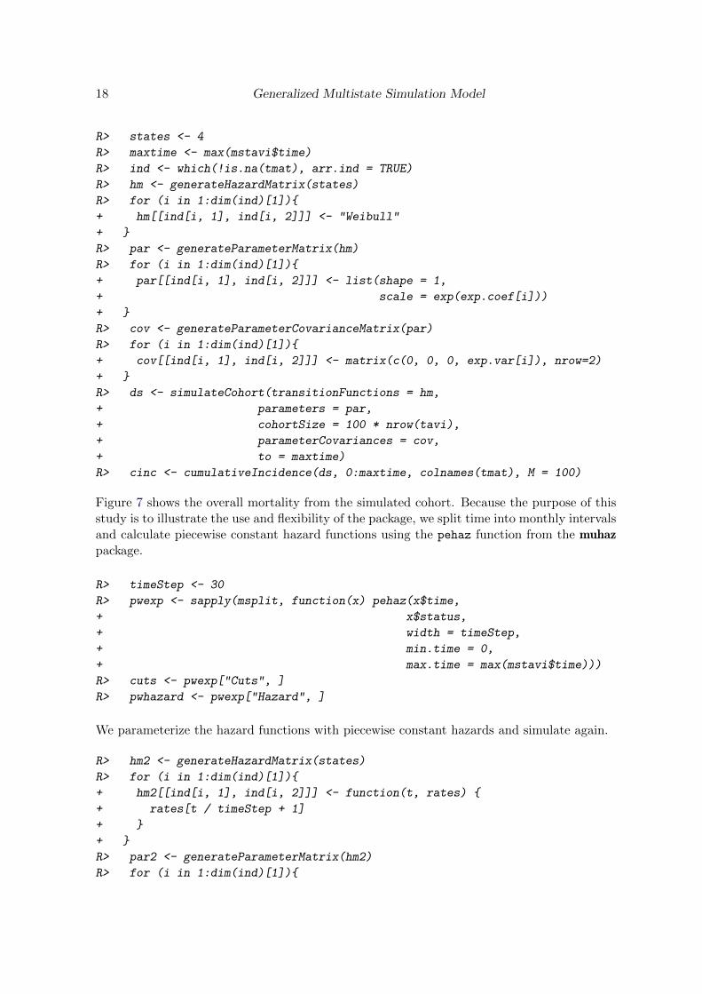
R> cinc <- cumulativeIncidence(ds, 0:maxtime, colnames(tmat), M = 100)
Figure 7 shows the overall mortality from the simulated cohort. Because the purpose of thisstudy is to illustrate the use and flexibility of the package, we split time into monthly intervalsand calculate piecewise constant hazard functions using the pehaz function from the muhazpackage.
R> plot(cinc2, states = 4, axes = FALSE, frame = TRUE, col = 3,
+ xlab = "", main = "", ci = TRUE)
R> axis(2); axis(4)
R> axis(1, at = (0:13*90)[0:6*2+1], labels = (0:13*3)[0:6*2+1])
R> legend(200, .8, c("Data",
+ "Simulation: exponential",
+ "Simulation: piecewise exponential"),
+ lty = 1, col = c(1:3), lwd = 2)
Figure 7 shows how the simulated cumulative incidence depends on the statistical model.The package gems admits the choice of any transition-specific hazard function. We will nowuse the second model with piecewise constant hazard functions to estimate the effect of anintervention on mortality.
4.3. Intervention modeling
Suppose there is a new intervention that dramatically reduces the probability of getting bleed-ing complications, and we are interested in the impact of this intervention on mortality. Forsimplicity, we assume that the intervention reduces the transition-specific hazard of bleedingcomplications by 80%. Then
Figure 8 shows that reducing bleeding complications by 80% decreases three-year mortalityby 18.5% from 43.3% to 35.3%.
22 Generalized Multistate Simulation Model
5. Conclusion
In this paper we have presented the R package gems, which allows simulation from a directedacyclic multistate model. The R package gems is a flexible tool for investigating and evaluatinghealth interventions. We have given detailed examples of the use of each function of gems,and an example of its use to evaluate the effect of reduced bleeding complications in TAVIpatients on mortality.
Several packages estimate and simulate Markov models, but we are not aware of any otherpackages that allow simulation from a multistate model with arbitrary transition-specifichazard functions. This flexibility in hazard functions improves its fit to data and allowsto more accurately estimate the effects of different interventions. This package’s inclusionof history-dependent transitions is also a major improvement on many traditional modelstructures.
The gems package has some limitations, including the fact that a DAG is required. Sometimesit is useful to have models in which patients can return to a previous state. If this featureis not frequently required, the problem can be resolved by repeating the state in a DAG.Otherwise a different model structure is needed. A further limitation is that higher flexibilityrequires more intensive computation, compared to traditional models. Longitudinal processescould be incorporated in a joint model, and evaluations of the artificial cohorts could befurther automated in future expansions.
The gems package has useful functions for simulating hypothetical cohorts of patients basedon a multistate model with general transition-specific hazard functions, and is a flexible anduser-friendly tool for planning and evaluating public-health interventions.
Acknowledgments
We would like to thank the Swiss Cardiovascular Center Bern at the Bern University Hospital(S. Windecker, B. Meier, P. Wenaweser, T. Pilgrim, S. Stortecky, L. Buellesfeld) for providingdata on transcatheter aortic valve implantation for the case study. We also thank K. Talfor her editorial assistance. This study was supported by UNITAID; a PROSPER fellowshipto O. Keiser and a PRODOC PhD grant for N. Blaser from the Swiss National ScienceFoundation.
References
Anderson RM, May RM (1992). Infectious Diseases of Humans Dynamics and Control. OxfordUniversity Press. URL http://www.oup.com/uk/catalogue/?ci=9780198540403.
Blaser N, Salazar Vizcaya L, Estill J, Zahnd C, Kalesan B, Egger M, Keiser O, Gsponer T(2015). “gems: An R Package for Simulating from Disease Progression Models.” Journal ofStatistical Software, 64(10), 1–22. URL http://www.jstatsoft.org/v64/i10/.
de Wreede LC, Fiocco M, Putter H (2011). mstate: An R Package for the Analysis ofCompeting Risks and Multi-State Models. URL http://www.jstatsoft.org/v38/i07/.
Estill J, Aubriere C, Egger M, Johnson L, Wood R, Garone D, Gsponer T, Wandeler G, BoulleA, Davies MA, Hallett TB, Keiser O (2012). “Viral Load Monitoring of AntiretroviralTherapy, Cohort Viral Load and HIV Transmission in Southern Africa: a MathematicalModelling Analysis.” AIDS, 26(11), 1403–13.
Estill J, Tweya H, Egger M, Wandeler G, Feldacker C, Johnson LF, Blaser N, Vizcaya LS, PhiriS, Keiser O (2014). “Tracing of Patients Lost to Follow-up and HIV Transmission: Mathe-matical Modeling Study Based on 2 Large ART Programs in Malawi.” J. Acquir. ImmuneDefic. Syndr., 65(5), e179–186. ISSN 1944-7884. doi:10.1097/QAI.0000000000000075.
Garnett GP, Cousens S, Hallett TB, Steketee R, Walker N (2011). “Mathematical Models inthe Evaluation of Health Programmes.” Lancet, 378(9790), 515–25.
Gazzola L, Tincati C, Bellistri GM, Monforte A, Marchetti G (2009). “The Absence ofCD4+ T Cell Count Recovery Despite Receipt of Virologically Suppressive Highly ActiveAntiretroviral Therapy: Clinical Risk, Immunological Gaps, and Therapeutic Options.”Clin Infect Dis, 48(3), 328–37.
Gillespie DT (1977). “Exact Stochastic Simulation of Coupled Chemical Reactions.” J. Phys.Chem., 81(25), 2340–2361. URL http://dx.doi.org/10.1021/j100540a008.
Hess K, Gentleman R (2010). muhaz: Hazard Function Estimation in Survival Analysis.R package version 1.2.5, URL http://CRAN.R-project.org/package=muhaz.
Jackson CH (2011). “Multi-State Models for Panel Data: The msm Package for R.” Journalof Statistical Software, 38(8), 1–29. URL http://www.jstatsoft.org/v38/i08/.
Ling D, Huang HZ, Liu Y (2009). “A method for parameter estimation of Mixed Weibulldistribution.” In Reliability and Maintainability Symposium, 2009. RAMS 2009. Annual,pp. 129–133. ISSN 0149-144X. doi:10.1109/RAMS.2009.4914663.
Lloyd AL (2001). “Realistic Distributions of Infectious Periods in Epidemic Models: ChangingPatterns of Persistence and Dynamics.” Theor Popul Biol, 60(1), 59–71.
Pearl J (2009). Causality. Second edition. Cambridge University Press, Cambridge. ISBN978-0-521-89560-6; 0-521-77362-8.
Phillips AN, Pillay D, Garnett G, Bennett D, Vitoria M, Cambiano V, Lundgren J (2011).“Effect on Transmission of HIV-1 Resistance of Timing of Implementation of Viral LoadMonitoring to Determine Switches from First to Second-line Antiretroviral Regimens inResource-limited Settings.” AIDS, 25(6), 843–50.
Pilgrim T, Kalesan B, Wenaweser P, Huber C, Stortecky S, Buellesfeld L, Khattab AA, EberleB, Gloekler S, Gsponer T, Meier B, Juni P, Carrel T, Windecker S (2012). “Predictors ofClinical Outcomes in Patients With Severe Aortic Stenosis Undergoing TAVI: A MultistateAnalysis.” Circ Cardiovasc Interv, 5(6), 856–61.
Salazar Vizcaya L, Blaser N, Gsponer T (2013). gems: General Multistate Simulation Model.R package version 0.9.1, URL http://CRAN.R-project.org/package=gems.
Therneau TM (2014). A Package for Survival Analysis in S. R package version 2.37-7, URLhttp://CRAN.R-project.org/package=survival.
Affiliation:
Nello BlaserInstitute of Social and Preventive MedicineUniversity of Bern3012 Bern, SwitzerlandE-mail: [email protected]
Luisa Salazar VizcayaInstitute of Social and Preventive MedicineUniversity of Bern3012 Bern, SwitzerlandE-mail: [email protected]