GENE EXPRESSION PROGRAMMING AND THE EVOLUTION OF COMPUTER PROGRAMS CÂNDIDA FERREIRA Gepsoft, 73 Elmtree Drive, Bristol BS13 8NA, UK [email protected]In Leandro N. de Castro and Fernando J. Von Zuben, eds., Recent Developments in Biologically Inspired Computing, pages 82-103, Idea Group Publishing, 2004. In this chapter an artificial problem solver inspired in natural genotype/phenotype sys- tems – gene expression programming – is presented. As an introduction, the fundamental differences between gene expression programming and its predecessors, genetic algorithms and genetic programming, are briefly summarized so that the evolutionary advantages of gene expression programming are better understood. The work proceeds with a detailed description of the architecture of the main players of this new algorithm (chromosomes and expression trees), focusing mainly on the interactions between them and how the simple yet revolutionary structure of the chromosomes allows the efficient, unconstrained exploration of the search space. And finally, the chapter closes with an advanced applica- tion in which gene expression programming is used to evolve computer programs for diagnosing breast cancer. 1. Evolutionary Algorithms in Problem Solving The way nature solves problems and creates complexity has inspired scientists to create artificial systems that learn by themselves how to solve a particular problem. The first at- tempts were done in the 1950s by Friedberg (Friedberg 1958; Friedberg et al. 1959), but ever since highly sophisticated systems have been developed that apply Darwin's ideas of natural evolution to the artificial world of computers and modeling. Of particular interest to this work are the genetic algorithms (GAs) and the genetic programming (GP) technique as they are the predecessors of gene expression programming (GEP), the most recent de- velopment in evolutionary computation and the theme of this chapter. A brief introduction to these three techniques is given below. 1.1. Genetic Algorithms Genetic algorithms were invented by John Holland in the 1960s and they also apply bio- logical evolution theory to computer systems (Holland 1975). Like all evolutionary com- puter systems, GAs are an oversimplification of biological evolution. In this case, solutions to a problem are usually encoded in strings of 0’s and 1’s (chromosomes), and populations
Transcript
GEP AND THE EVOLUTION OF COMPUTER PROGRAMS | 1
GENE EXPRESSION PROGRAMMING AND THEEVOLUTION OF COMPUTER PROGRAMS
In Leandro N. de Castro and Fernando J. Von Zuben, eds., Recent Developments inBiologically Inspired Computing, pages 82-103, Idea Group Publishing, 2004.
In this chapter an artificial problem solver inspired in natural genotype/phenotype sys-tems – gene expression programming – is presented. As an introduction, the fundamentaldifferences between gene expression programming and its predecessors, genetic algorithmsand genetic programming, are briefly summarized so that the evolutionary advantages ofgene expression programming are better understood. The work proceeds with a detaileddescription of the architecture of the main players of this new algorithm (chromosomesand expression trees), focusing mainly on the interactions between them and how thesimple yet revolutionary structure of the chromosomes allows the efficient, unconstrainedexploration of the search space. And finally, the chapter closes with an advanced applica-tion in which gene expression programming is used to evolve computer programs fordiagnosing breast cancer.
1. Evolutionary Algorithms in Problem Solving
The way nature solves problems and creates complexity has inspired scientists to createartificial systems that learn by themselves how to solve a particular problem. The first at-tempts were done in the 1950s by Friedberg (Friedberg 1958; Friedberg et al. 1959), butever since highly sophisticated systems have been developed that apply Darwin's ideas ofnatural evolution to the artificial world of computers and modeling. Of particular interestto this work are the genetic algorithms (GAs) and the genetic programming (GP) techniqueas they are the predecessors of gene expression programming (GEP), the most recent de-velopment in evolutionary computation and the theme of this chapter. A brief introductionto these three techniques is given below.
1.1. Genetic Algorithms
Genetic algorithms were invented by John Holland in the 1960s and they also apply bio-logical evolution theory to computer systems (Holland 1975). Like all evolutionary com-puter systems, GAs are an oversimplification of biological evolution. In this case, solutionsto a problem are usually encoded in strings of 0’s and 1’s (chromosomes), and populations
2 | C FERREIRA
of such strings (individuals or candidate solutions) are used in order to evolve a good solu-tion to a particular problem. From generation to generation candidate solutions are repro-duced with modification and selected according to fitness. Modification in the original GAwas introduced by the genetic operators of mutation, crossover, and inversion.
It is worth pointing out that GAs’ individuals consist of naked chromosomes or, in otherwords, GAs’ individuals are simple replicators. And like all simple replicators, the chro-mosomes of genetic algorithms function simultaneously as genotype and phenotype: theyare both the object of selection and the guardians of the genetic information that must bereplicated and passed on with modification to the next generation. Consequently, the wholestructure of the replicator determines the functionality and, therefore, the fitness of the in-dividual. For instance, in such systems it would not be possible to use only a particularregion of the replicator as a solution to a problem: the whole replicator is always the solu-tion: nothing more, nothing less.
1.2. Genetic Programming
Genetic programming, invented by Cramer in 1985 (Cramer 1985) and further developedby Koza (1992), solves the problem of fixed length solutions through the use of nonlinearstructures (parse trees) with different sizes and shapes. The alphabet used to create thesestructures is also more varied, creating a richer, more versatile system of representation.Notwithstanding, the created individuals also lack a simple, autonomous genome. Like thelinear chromosomes of genetic algorithms, the nonlinear structures of GP are also cursedwith the dual role of genotype/phenotype.
The parse trees of genetic programming resemble protein molecules in their use of aricher alphabet and in their complex and unique hierarchical representation. Indeed, parsetrees are capable of exhibiting a great variety of functionalities. The problem with thesecomplex replicators is that their reproduction with modification is highly constrained inevolutionary terms because the modifications must take place on the parse tree itself and,consequently, only a limited range of modification is possible. Indeed, special kinds of ge-netic operators were developed that operate at the tree level, modifying or exchanging par-ticular branches between trees.
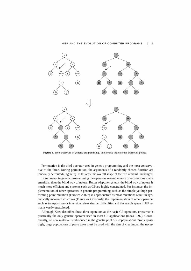
Although at first sight this might appear advantageous, it greatly limits this technique(we all know the limits of grafting and pruning in nature). Consider for instance crossover,the most used and often the only search operator used in genetic programming. In this case,selected branches are exchanged between two parent trees to create offspring (Figure 1).The idea behind its implementation was to exchange smaller, mathematically concise blocksin order to evolve more complex, hierarchical solutions composed of smaller building blocks.
The mutation operator in GP is also very different from natural point mutation. Thisoperator selects a node in the parse tree and replaces the branch underneath by a new ran-domly generated branch (Figure 2). Notice that the overall shape of the tree is not greatlychanged by this kind of mutation, especially if lower nodes are preferentially chosen asmutation targets.
GEP AND THE EVOLUTION OF COMPUTER PROGRAMS | 3
Permutation is the third operator used in genetic programming and the most conserva-tive of the three. During permutation, the arguments of a randomly chosen function arerandomly permuted (Figure 3). In this case the overall shape of the tree remains unchanged.
In summary, in genetic programming the operators resemble more of a conscious math-ematician than the blind way of nature. But in adaptive systems the blind way of nature ismuch more efficient and systems such as GP are highly constrained. For instance, the im-plementation of other operators in genetic programming such as the simple yet high-per-forming point mutation (Ferreira 2002c) is unproductive as most mutations result in syn-tactically incorrect structures (Figure 4). Obviously, the implementation of other operatorssuch as transposition or inversion raises similar difficulties and the search space in GP re-mains vastly unexplored.
Although Koza described these three operators as the basic GP operators, crossover ispractically the only genetic operator used in most GP applications (Koza 1992). Conse-quently, no new material is introduced in the genetic pool of GP populations. Not surpris-ingly, huge populations of parse trees must be used with the aim of creating all the neces-
Figure 1. Tree crossover in genetic programming. The arrows indicate the crossover points.
ba
a
a
b
b
b
b
sqrt
ba
sqrt
sqrt
sqrt
b a
a
a a a
a
b
b
b
b
sqrt
sqrt
sqrt
sqrt
b
a a
4 | C FERREIRA
Figure 4. Illustration of a hypothetical event of point mutation in genetic programming.The arrow indicates the mutation point. Note that the daughter tree is an invalid structure.
a a
b b
b b b
b
sqrt
Figure 2. Tree mutation in genetic programming. The arrow indicates the mutation point. Thenew branch randomly generated by the mutation operator in the daughter tree is shown in gray.
a b
a b
sqrt
sqrt
a
b
a b
sqrt
Figure 3. Permutation in genetic programming. The arrow indicates the permutation point.Note that the arguments of the permuted function traded places in the daughter tree.
a aa ab b
b
sqrt
b
sqrt
sary building blocks with the inception of the initial population in order to guarantee thediscovery of a good solution only by moving the initial building blocks around.
Finally, due to the dual function of the parse trees (genotype and phenotype), geneticprogramming is incapable of a simple, rudimentary expression: in all cases, the entire parsetree is the solution.
GEP AND THE EVOLUTION OF COMPUTER PROGRAMS | 5
1.3. Gene Expression Programming
Gene expression programming was invented by myself in 1999 (Ferreira 2001), and incor-porates both the simple, linear chromosomes of fixed length similar to the ones used ingenetic algorithms and the ramified structures of different sizes and shapes similar to theparse trees of genetic programming. This is equivalent to say that in gene expression pro-gramming the genotype and phenotype are finally separated and the system can now ben-efit from all the advantages this brings about.
Thus, the phenotype of GEP consists of the same kind of ramified structure used in ge-netic programming. But the ramified structures created by GEP (expression trees) are theexpression of a totally autonomous genome. Therefore, with gene expression programming,the second evolutionary threshold – the phenotype threshold – is crossed (Dawkins 1995).This means that, during reproduction, only the genome (slightly modified) is passed on tothe next generation and we no longer need to replicate and mutate rather cumbersome struc-tures: all the modifications take place in a simple linear structure which only later will growinto an expression tree.
The fundamental steps of gene expression programming are schematically representedin Figure 5. The process begins with the random generation of the chromosomes of a cer-tain number of individuals (the initial population). Then these chromosomes are expressedand the fitness of each individual is evaluated against a set of fitness cases (also calledselection environment). The individuals are then selected according to their fitness (theirperformance in that particular environment) to reproduce with modification, leaving prog-eny with new traits. These new individuals are, in their turn, subjected to the same devel-opmental process: expression of the genomes, confrontation of the selection environment,selection, and reproduction with modification. The process is repeated for a certain numberof generations or until a good solution has been found.
The pivotal insight of gene expression programming consisted in the invention of chro-mosomes capable of representing any parse tree. For that purpose a new language – Karvalanguage – was created in order to read and express the information encoded in the chro-mosomes. The details of this new language are given in the next section.
Furthermore, the structure of the chromosomes was designed to allow the creation ofmultiple genes, each coding for a smaller program or sub-expression tree. It is worth em-phasizing that gene expression programming is the only genetic algorithm with multiplegenes. Indeed, the creation of more complex individuals composed of multiple genes isextremely simplified in truly functional genotype/phenotype systems. In fact, after their in-ception, these systems seem to catapult themselves into higher levels of complexity such asthe multicellular systems, where different cells put together different consortiums of genes(Ferreira 2002a).
The basis for all this novelty resides on the revolutionary structure of GEP genes. Thesimple but plastic structure of these genes not only allows the encoding of any conceivableprogram but also allows their efficient evolution. Due to this versatile structural organiza-tion, a very powerful set of genetic operators can be easily implemented and used to search
6 | C FERREIRA
Figure 5. The flowchart of gene expression programming.
Create Chromosomes of Initial Population
End
Express Chromosomes
Execute Each Program
Evaluate Fitness
Replication
Prepare New Chromosomes of Next Generation
Keep Best Program
Select Programs
Genetic Modification
Iterate or Terminate?
Terminate
Iterate
Reproduction
very efficiently the solution space. As in nature, the search operators of gene expressionprogramming always produce valid structures and therefore are remarkably suited to creat-ing genetic diversity.
2. The Architecture of GEP Individuals
We know already that the main players in gene expression programming are the chromo-somes and the expression trees (ETs), being the latter the expression of the genetic infor-mation encoded in the former. As in nature, the process of information decoding is calledtranslation. And this translation implies obviously a kind of code and a set of rules. Thegenetic code is very simple: a one-to-one relationship between the symbols of the chromo-some and the nodes they represent in the trees. The rules are also very simple: they deter-mine the spatial organization of nodes in the expression trees and the type of interactionbetween sub-ETs. Therefore, there are two languages in GEP: the language of the genes
GEP AND THE EVOLUTION OF COMPUTER PROGRAMS | 7
and the language of expression trees and, thanks to the simple rules that determine the struc-ture of ETs and their interactions, we will see that it is possible to infer immediately thephenotype given the sequence of a gene, and vice versa. This means that we can choose tohave a very complex program represented by its compact genome without losing in mean-ing. This unequivocal bilingual notation is called Karva language. Its details are explainedin the remainder of this section.
2.1. Open Reading Frames and Genes
The structural organization of GEP genes is better understood in terms of open readingframes (ORFs). In biology, an ORF or coding sequence of a gene begins with the startcodon, continues with the amino acid codons, and ends at a termination codon. However, agene is more than the respective ORF, with sequences upstream of the start codon and se-quences downstream of the stop codon. Although in GEP the start site is always the firstposition of a gene, the termination point does not always coincide with the last position ofa gene. Consequently, it is common for GEP genes to have non-coding regions downstreamof the termination point. (For now we will not consider these non-coding regions, as theydo not interfere with expression.)
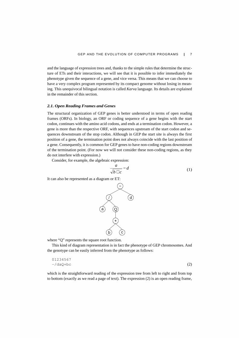
Consider, for example, the algebraic expression:
(1)
It can also be represented as a diagram or ET:
a
d
b c
Q
where “Q” represents the square root function.This kind of diagram representation is in fact the phenotype of GEP chromosomes. And
the genotype can be easily inferred from the phenotype as follows:
01234567-/daQ+bc (2)
which is the straightforward reading of the expression tree from left to right and from topto bottom (exactly as we read a page of text). The expression (2) is an open reading frame,
dcb
a −+
8 | C FERREIRA
starting at “-” (position 0) and terminating at “c” (position 7). These open reading frameswere named K-expressions from Karva language.
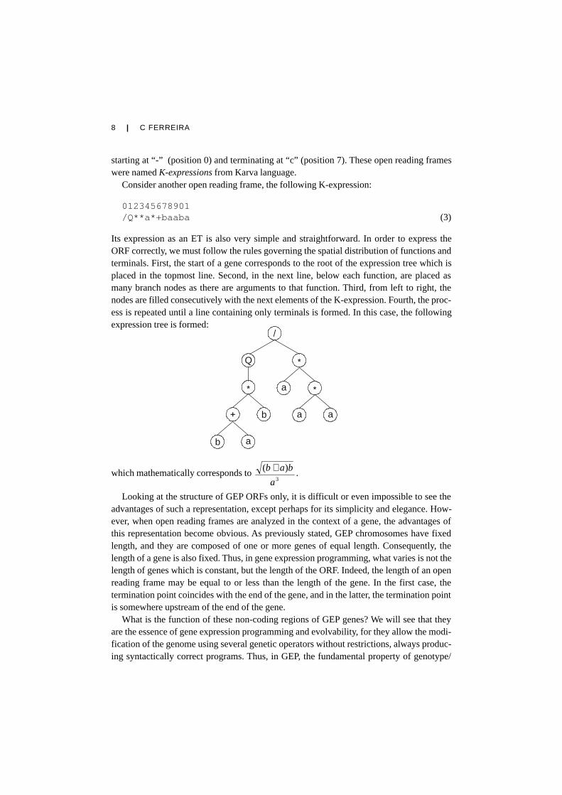
Consider another open reading frame, the following K-expression:
012345678901/Q**a*+baaba (3)
Its expression as an ET is also very simple and straightforward. In order to express theORF correctly, we must follow the rules governing the spatial distribution of functions andterminals. First, the start of a gene corresponds to the root of the expression tree which isplaced in the topmost line. Second, in the next line, below each function, are placed asmany branch nodes as there are arguments to that function. Third, from left to right, thenodes are filled consecutively with the next elements of the K-expression. Fourth, the proc-ess is repeated until a line containing only terminals is formed. In this case, the followingexpression tree is formed:
b
b
a
aa
a
Q
which mathematically corresponds to 3
)(
a
bab + .
Looking at the structure of GEP ORFs only, it is difficult or even impossible to see theadvantages of such a representation, except perhaps for its simplicity and elegance. How-ever, when open reading frames are analyzed in the context of a gene, the advantages ofthis representation become obvious. As previously stated, GEP chromosomes have fixedlength, and they are composed of one or more genes of equal length. Consequently, thelength of a gene is also fixed. Thus, in gene expression programming, what varies is not thelength of genes which is constant, but the length of the ORF. Indeed, the length of an openreading frame may be equal to or less than the length of the gene. In the first case, thetermination point coincides with the end of the gene, and in the latter, the termination pointis somewhere upstream of the end of the gene.
What is the function of these non-coding regions of GEP genes? We will see that theyare the essence of gene expression programming and evolvability, for they allow the modi-fication of the genome using several genetic operators without restrictions, always produc-ing syntactically correct programs. Thus, in GEP, the fundamental property of genotype/
GEP AND THE EVOLUTION OF COMPUTER PROGRAMS | 9
phenotype systems – syntactic closure – is intrinsic, allowing the totally unconstrained re-structuring of the genotype and, consequently, an efficient evolution.
In the next section we are going to analyze the structural organization of GEP genes inorder to understand how they invariably code for syntactically correct programs and whythey allow an unconstrained application of virtually any genetic operator.
2.2. Structural Organization of Genes
The genes of gene expression programming are composed of a head and a tail. The headcontains symbols that represent both functions and terminals, whereas the tail contains onlyterminals. For each problem, the length of the head h is chosen, whereas the length of thetail t is a function of h and the number of arguments n of the function with more arguments(also called maximum arity) and is evaluated by the equation:
t = h (n-1) + 1 (4)
Consider a gene for which the set of functions F = {Q, *, /, -, +} and the set of terminalsT = {a, b}. In this case n = 2; if we chose an h = 11, then t = 11 (2 - 1) + 1 = 12; thus, thelength of the gene g is 11 + 12 = 23. One such gene is shown below (the tail is shown inbold):
which mathematically corresponds to the expression ( )1−ab . In this case, the termina-
tion point shifts four positions to the right (position 13), enlarging and changing signifi-cantly the daughter tree.
Obviously the opposite also might happen, and the daughter tree might shrink. For ex-ample, consider again gene (5) above, and suppose a mutation occurred at position 1, chang-ing the “-” into “a”:
In this case, the ORF ends at position 2, shortening the original ET in seven nodes.So, despite their fixed length, each gene has the potential to code for expression trees of
different sizes and shapes, where the simplest is composed of only one node (when the firstelement of a gene is a terminal) and the largest is composed of as many nodes as the lengthof the gene (when all the elements of the head are functions with maximum arity).
It is evident from the examples above, that any modification made in the genome, nomatter how profound, always results in a structurally correct program. Obviously, the struc-tural organization of genes must be preserved, always maintaining the boundaries betweenhead and tail. We will be able to fully appreciate the plasticity of GEP chromosomes in thesection Genetic Operators and Evolution where the mechanisms and effects of differentgenetic operators will be thoroughly analyzed.
GEP AND THE EVOLUTION OF COMPUTER PROGRAMS | 11
2.3. Multigenic Chromosomes
The chromosomes of gene expression programming are usually composed of more thanone gene of equal length. For each problem or run, the number of genes, as well as thelength of the head, are a priori chosen. Each gene codes for a sub-ET and the sub-ETsinteract with one another forming a more complex multi-subunit expression tree.
Consider, for example, the following chromosome with length 39, composed of threegenes, each with length 13 (the tails are shown in bold):
It has three open reading frames, and each ORF codes for a sub-ET (Figure 6). The start ofeach ORF is always given by position 0; the end of each ORF, though, is only evident uponconstruction of the corresponding sub-ET. As shown in Figure 6, the first open readingframe ends at position 9; the second ORF ends at position 5; and the last ORF ends atposition 2. Thus, GEP chromosomes contain several ORFs of different sizes, each ORFcoding for a structurally and functionally unique sub-ET. Depending on the problem at hand,these sub-ETs may be selected individually depending on their respective outputs, or theymay form a more complex, multi-subunit expression tree and be selected as a whole. Inthese multi-subunit structures, individual sub-ETs interact with one another by a particularkind of posttranslational interaction or linking. For instance, algebraic sub-ETs can be linkedby addition or multiplication whereas Boolean sub-ETs can be linked by OR, AND or IF.
The linking of three sub-ETs by addition is illustrated in Figure 6, c. Note that the finalET could be linearly encoded as the following K-expression:
012345678901234567890++/*-baQba++Qb*/abbba (9)
However, the use of multigenic chromosomes is more appropriate to evolve solutions tocomplex problems, for they permit the modular construction of complex, hierarchical struc-tures, where each gene codes for a smaller and simpler building block. These smaller buildingblocks are separated from each other, and thus can evolve independently. Not surprisingly,these multigenic systems are much more efficient than unigenic ones (Ferreira 2001, 2002a).
3. Genetic Operators and Evolution
Genetic operators are the core of all evolutionary algorithms, and two of them are commonto all evolutionary systems: selection and replication. Indeed, all artificial systems use ascheme to select individuals more or less according to fitness. Some schemes are totallydeterministic, whereas others include a touch of unpredictability. Gene expression program-ming uses one of the latter, namely, a fitness proportionate roulette-wheel scheme (see e.g.Goldberg 1989) coupled with the cloning of the best individual (simple elitism) as it mim-ics nature very faithfully and produces very good results.
12 | C FERREIRA
Figure 6. Expression of GEP genes as sub-ETs. a) A three-genic chromosome with the tails shown inbold. Position zero marks the start of each gene. b) The sub-ETs codified by each gene, which corre-
spond respectively to abbb /2 + , ( )baa +− , and ab / . c) The result of posttranlational linking with
addition, which obviously corresponds to ( ) abbaaabbb //2 ++−++ . The linking functions are
Thus, according to fitness and the luck of the draw, individuals are selected to be repli-cated. Although crucial, replication is the most uninteresting operator. During replication,chromosomes are dully copied and passed on to the next generation. The fitter the indi-vidual the higher the probability of passing on its genes to the next generation. So, duringreplication, the genomes of the selected individuals are copied every time the roulette picksthem up. And the roulette is spun as many times as there are individuals in the populationso that the same population size is maintained from generation to generation.
Although the center of the storm, by themselves, selection and replication, do nothing interms of adaptation. In fact, by themselves they can only cause genetic drift, makingpopulations less and less diverse with time until all the individuals are exactly the same.So, the corner stone of all evolutionary systems is genetic modification. And different algo-rithms create this modification differently. For instance, genetic algorithms normally usemutation and recombination; genetic programming uses almost exclusively tree recombi-nation; and gene expression programming uses mutation, inversion, transposition, and re-combination.
With the exception of GP, which is severely constrained in terms of tools of geneticmodification, in both GAs and GEP it is possible to implement easily a vast set of searchoperators because the search operators act on simple linear chromosomes. In fact, a variedset of search operators was implemented in gene expression programming in order to shedsome light on the dynamics of evolutionary systems, but what is important is to provide forthe necessary degree of genetic diversification in order to allow an efficient evolution. Nev-ertheless, mutation (by far the most efficient operator) by itself is capable of wonders. How-ever, the interplay of mutation with other operators not only allows an efficient evolutionbut also allows the duplication of genes and their subsequent differentiation, the creationof small repetitive sequences, and so forth, making things really interesting.
In the remainder of this section we will see how the search operators work and how theirimplementation in gene expression programming is a child’s play due to the simple factthat the genome is completely autonomous and consequently is not tied up in the structuralcomplexities of the computer programs encoded within.
3.1. Mutation
In gene expression programming, mutations can occur anywhere in the chromosome. How-ever, the structural organization of chromosomes must remain intact, that is, in the heads ofgenes any symbol can change into another (function or terminal), whereas in the tails ter-minals can only change into terminals. This way, the structural organization of chromo-somes is preserved, and all the new individuals produced by mutation are structurally cor-rect programs.
Suppose a mutation changed the “*” at position 5 in gene 1 to “a”; the “-” at position 1 ingene 2 to “Q”; and the “a” at position 2 in gene 3 to “*”. In this case the following chromo-some is obtained:
Note that if a function is mutated into a terminal or vice versa, or a function of oneargument is mutated into a function of two arguments or vice versa, the expression tree isusually modified drastically. Note also that the mutation on gene 1 is an example of a neu-tral mutation, as it occurred in the non-coding region of the gene. It is worth emphasizingthat the non-coding regions of GEP chromosomes are ideal places for the accumulation ofneutral mutations which are known to play an important role in evolution (Kimura 1983;Ferreira 2002b).
In summary, in gene expression programming there are no constraints both in the kindof mutation and the number of mutations in a chromosome as, in all cases, the newly cre-ated individuals are syntactically correct programs.
3.2. Inversion
We know already that the modifications bound to make a big impact occur usually in theheads of genes. Therefore, the inversion operator was restricted to these regions. Here anysequence might be randomly selected and inverted.
In gene expression programming, the inversion operator randomly chooses the chromo-some, the gene to be modified, and the start and termination points of the sequence to beinverted. It is worth pointing out that this is the first time the inversion operator is describedin gene expression programming.
Consider, for instance, the following three-genic chromosome:
It is worth pointing out that, since the inversion operator was restricted to the heads ofgenes, there is no danger of a function ending up in the tails and, consequently, all the newindividuals created by inversion are syntactically correct programs.
GEP AND THE EVOLUTION OF COMPUTER PROGRAMS | 15
3.3. Transposition and Insertion Sequence Elements
The transposable elements (also called transposons) of gene expression programming arefragments of the genome that can be activated and then jump to another place in the chro-mosome. In GEP there are three kinds of transposable elements: (1) short fragments with afunction or terminal in the first position that transpose to the head of genes except the root(insertion sequence elements or IS elements); (2) short fragments with a function in thefirst position that transpose to the start position of genes (root IS elements or RIS elements);(3) and entire genes that transpose to the beginning of chromosomes.
3.3.1. IS Transposition
Any sequence in the genome might become an IS element and, therefore, these elementsare randomly selected throughout the chromosome. A copy of the transposon is made andinserted at any position in the head of a gene, except the first position. The transpositionoperator randomly chooses the chromosome, the start and termination points of the IS ele-ment, and the target site. It is worth pointing out that the implementation of this operator asdescribed here, slightly differs from the original implementation (Ferreira 2001) where thelength of the IS elements was a priori chosen.
Suppose that the sequence “a/-” in gene 3 (positions 3-5) was picked up as an IS element tobe then inserted between positions 1-2 in gene 2, obtaining:
Note that, in this case, a perfect copy of the transposon appears at the site of insertion.Note also that a sequence with as many symbols as the IS element is deleted at the end ofthe head (in this case, the sequence “a*a” was deleted). Thus, despite this insertion, thestructural organization of chromosomes is maintained and, therefore, all the new individu-als created by IS transposition are syntactically correct programs.
3.3.2. Root Transposition
All root IS elements start with a function, and therefore must be chosen among the se-quences of the heads. For that, a point is randomly chosen in the head and the gene isscanned downstream until a function is found. This function becomes the start position ofthe RIS element. If no functions are found, the operator does nothing.
The RIS transposition operator randomly chooses the chromosome, the gene to be modi-fied, and the start and termination points of the RIS element. It is worth noticing that this
16 | C FERREIRA
operator is slightly different from the original RIS transposition (Ferreira 2001) as the lengthof the transposon is randomly chosen by this simpler RIS transposition.
Suppose that the sequence “/+b” in gene 1 was randomly chosen to become an RIS ele-ment. The transposon copies itself and then transposes to the root of the gene, giving:
Note that during transposition, the whole head shifts to accommodate the RIS element,losing, at the same time, the last symbols of the head (as many as there are in thetransposon). In this case, the sequence “+b*” was deleted and the transposon becameonly partially duplicated. As with IS transposition, the tail of the gene subjected to RIStransposition and all nearby genes remain unchanged. Note, again, that all the programsnewly created by this operator are syntactically correct as it also preserves the structuralorganization of the chromosome.
3.3.3. Gene Transposition
In gene transposition an entire gene works as a transposon and transposes itself to the be-ginning of the chromosome. In contrast to the other forms of transposition, in gene trans-position, the transposon (the gene) is deleted at the place of origin.
The gene transposition operator randomly chooses the chromosome to be modified andthen randomly chooses one of its genes (except the first, obviously) to transpose. Considerthe following chromosome composed of three genes:
Apparently, gene transposition is only capable of shuffling genes and, for sub-ETs linkedby commutative functions, this contributes nothing to adaptation in the short run. Note,however, that when the sub-ETs are linked by a non-commutative function, the order of the
GEP AND THE EVOLUTION OF COMPUTER PROGRAMS | 17
genes matters and, in this case, gene transposition becomes a macromutator. However, genetransposition becomes particularly interesting when it is used in conjunction with recombi-nation, for it allows not only the duplication of genes but also a more generalized shufflingof genes or smaller building blocks.
3.4. Recombination
In gene expression programming there are three kinds of recombination: one-point recom-bination, two-point recombination, and gene recombination. In all types of recombination,two chromosomes are randomly chosen and paired to exchange some material between them,creating two new daughter chromosomes.
3.4.1. One-point Recombination
In one-point recombination the parent chromosomes are paired and split up at exactly thesame point. The material downstream of the recombination point is afterwards exchangedbetween the two chromosomes.
Consider the following parent chromosomes, each composed of three genes:
Suppose bond 4 in gene 2 (between positions 3 and 4) was randomly chosen as the crosso-ver point. Then, the paired chromosomes are both cut at this bond, and exchange betweenthem the material downstream of the crossover point, forming the offspring below:
It is worth emphasizing that GEP chromosomes can cross over any point in the genome,continually disrupting old building blocks and continually forming new ones. Furthermore,due to both the multigenic nature of GEP chromosomes and the existence of non-codingregions in most genes, entire genes and intact open reading frames can be swapped be-tween parent chromosomes. Thus, the disruptive tendencies of one-point recombination(splitting of building blocks) coexist side by side with its more conservative tendencies(swapping of genes and ORFs), making one-point recombination (and of course two-pointrecombination too) a very well balanced genetic operator. Furthermore, like all the otherrecombinational operators, when one-point recombination is used together with gene trans-position, it is also capable of duplicating genes.
18 | C FERREIRA
3.4.2. Two-point Recombination
In two-point recombination two parent chromosomes are paired side by side and twopoints are randomly chosen as crossover points. The material between the recombina-tion points is afterwards exchanged between the parent chromosomes, forming two newdaughter chromosomes.
Consider the following pair of recombining chromosomes:
Suppose bond 7 in gene 1 (between positions 6 and 7) and bond 4 in gene 3 (betweenpositions 3 and 4) were chosen as crossover points. Then, the following daughter chromo-somes are created:
It is worth emphasizing that two-point recombination is more disruptive than one-pointrecombination in the sense that it recombines the genetic material more thoroughly, con-stantly destroying old building blocks and creating new ones. But like one-point recombi-nation, two-point recombination has also a conservative side and it is good at swappingentire genes and open reading frames. And, as observed for one-point recombination, two-point recombination can also give rise to duplicated genes if it were used together withgene transposition.
Notwithstanding, if the goal is to evolve good solutions, one-point or two-point recom-bination should never be used as the only source of genetic variation as they tend to ho-mogenize populations (Ferreira 2002c). However, together with mutation, inversion andtransposition, these operators are an excellent source of genetic variation and are more thansufficient to evolve good solutions to virtually all problems.
3.4.3. Gene Recombination
In the third kind of GEP recombination, entire genes are exchanged between two parentchromosomes, forming two daughter chromosomes containing genes from both parents.The exchanged genes are randomly chosen and occupy exactly the same position in theparent chromosomes.
Note that, with this kind of recombination, similar genes can be exchanged but, most of thetimes, the exchanged genes are very different from one another and new material is intro-duced in the population.
It is worth emphasizing that this operator is unable to create new genes: the individualscreated by gene recombination are different arrangements of existing genes. Obviously, ifgene recombination were used as the unique source of genetic variation, more complexproblems could only be solved using very large initial populations in order to provide forthe necessary diversity of genes. However, GEP evolvability is based not only in the shuf-fling of genes (achieved by gene recombination and gene transposition), but also in theconstant creation of new genetic material which is carried out essentially by mutation, in-version and transposition (both IS and RIS transposition) and, to a lesser extent, by recom-bination (both one-point and two-point recombination).
4. Evolving Computer Programs for Diagnosing Breast Cancer
In this section we are going to use gene expression programming to design a computerprogram that can be used to diagnose breast cancer. The data sets used both for trainingand testing were obtained from PROBEN1 – a set of neural network benchmark problemsand benchmarking rules (Prechelt 1994). Both the technical report and the data sets areavailable through anonymous FTP from Neural Bench archive at Carnegie Mellon Univer-sity (machine ftp.cs.cmu.edu, directory /afs/cs/project/connect/bench/contrib/prechelt)and from the machine ftp.ira.uka.de in directory /pub/neuron. The file name in both casesis proben1.tar.gz.
In this diagnosis task the goal is to classify a tumor as either benign (0) or malignant (1)based on nine different cell analysis (input attributes or terminals).
The model presented here was obtained using the cancer1 data set of PROBEN1 wherethe binary 1-of-m encoding in which each bit represents one of m-possible output classeswas replaced by a 1-bit encoding (“0” for benign and “1” for malignant). The first 350samples were used for training and the last 174 were used to test the performance of themodel in real use. This means that absolutely no information from the test set samples orthe test set performance are available during the adaptive process. Thus, both the classifi-cation accuracy and classification error on the test set can be used to evaluate the generali-zation performance of the evolved models.
For this problem a very simple function set was chosen, composed only of the four arith-metic operators, that is, F = {+, -, *, /}, where each function was weighted five times; theset of terminals consisted of the nine attributes used in this problem and were represented
20 | C FERREIRA
by T = {d0, ..., d
8} which correspond, respectively, to clump thickness, uniformity of cell
size, uniformity of cell shape, marginal adhesion, single epithelial cell size, bare nuclei,bland chromatin, normal nucleoli, and mitoses.
In classification problems where the output is often binary, it is important to set criteriato convert real-valued numbers into zero or one. This is the 0/1 rounding threshold R
t that
converts the output of a chromosome into “1” if the output is equal to or greater than Rt, or
into “0” otherwise. For this problem we are going to use Rt = 0.1.
The fitness function used to evaluate the performance of each candidate model is verysimple and is based on the number of samples correctly classified. Thus, the fitness f
i of an
individual program corresponds to the number of hits and is evaluated by the formula:
if n > Cp, then f
i = n; else f
i = 0 (10)
where n is the number of sample cases correctly evaluated, and Cp is the number of sam-
ples in the class with more members (predominant class).As it is customary in genetic programming (Koza 1992) and gene expression program-
ming (Ferreira 2001), the parameters used per run are summarized in a table (Table 1).Note that, in this case, a small population of 50 individuals and chromosomes composed ofthree genes with an h = 8 and sub-ETs linked by addition were used. The program below
Table 1Settings used in the breast cancer problem.
Number of generations 500
Population size 50
Number of training samples 350
Number of testing samples 174
Function set (+-*/)5
Terminal set d0 - d9
Rounding threshold 0.1
Head length 8
Number of genes 3
Linking function +
Chromosome length 51
Mutation rate 0.044
Inversion rate 0.1
IS transposition rate 0.1
RIS transposition rate 0.1
One-point recombination rate 0.3
Two-point recombination rate 0.3
Gene recombination rate 0.1
Gene transposition rate 0.1
GEP AND THE EVOLUTION OF COMPUTER PROGRAMS | 21
was discovered after 423 generations (genes are shown separately and a dot is used to sepa-rate each element):
It has a fitness of 340 evaluated against the training set of 350 fitness cases and maximumfitness on the test set of 174 examples. This means that this model is very good indeed,with a classification accuracy of 100% and a classification error of 0% in the test set. In thetraining set a classification accuracy of 97.14% and a classification error of 2.86% wereobtained.
Note that for the expression of chromosome (11a) to be complete the sub-ETs must belinked by addition and the 0/1 rounding threshold must be taken into account. With thesoftware APS 3.0 by Gepsoft, the model (11a) above can be automatically converted into afully expressed computer program or function, such as the C++ function below:
Similarly, all models evolved by gene expression programming can be immediately con-verted into virtually any programming language through the use of grammars, includingthe universal representation of parse trees (Figure 7). These trees can then be used to graspimmediately the mathematical intricacies of the evolved models and therefore are ideal forextracting knowledge from data.
As you can clearly see in Figure 7, all the cell analysis seem to be relevant to an accu-rate diagnosis of breast cancer. This is, indeed, one of the great advantages of gene expres-sion programming: the possibility of extracting knowledge almost instantaneously as themodels evolved by GEP can be represented in any conceivable language, including theuniversal diagram representation of expression trees.
5. Conclusions
In this chapter the details of implementation of gene expression programming were thor-oughly explained, giving other researchers the possibility of implementing it themselves.Furthermore, this new algorithm was summarily compared to genetic algorithms and ge-netic programming in order to bring into focus the fundamental differences between thethree techniques and, consequently, enable readers to appreciate the advantages a full-fledged
22 | C FERREIRA
Figure 7. The sub-ETs of the model (11b) evolved by gene expression programming to diagnose breastcancer. (Expression trees drawn by Gepsoft APS 3.0.)
genotype/phenotype system brings into evolutionary computation. In addition, the classifi-cation task solved in this work clearly demonstrates the modeling prowess of this new tech-nique: the compact computer programs evolved by gene expression programming in itsnative Karva code can be immediately used to generate highly sophisticated computer pro-grams in virtually any programming language through the use of grammars as is alreadydone in commercially available software.
GEP AND THE EVOLUTION OF COMPUTER PROGRAMS | 23
Bibliography
Cramer, N. L. (1985). A Representation for the Adaptive Generation of Simple SequentialPrograms. In J. J. Grefenstette, ed., Proceedings of the First International Conference onGenetic Algorithms and Their Applications, Erlbaum.
Dawkins, R. (1995). River out of Eden, Weidenfeld and Nicolson.
Ferreira, C. (2001). Gene Expression Programming: A New Adaptive Algorithm for SolvingProblems. Complex Systems, 13 (2): 87-129.
Ferreira, C. (2002a). Gene Expression Programming: Mathematical Modeling by an Artifi-cial Intelligence, Angra do Heroísmo, Portugal.
Ferreira, C. (2002b). Genetic Representation and Genetic Neutrality in Gene Expression Pro-gramming. Advances in Complex Systems, 5 (4): 389-408.
Ferreira, C. (2002c). Mutation, Transposition, and Recombination: An Analysis of the Evolu-tionary Dynamics. In H. J. Caulfield, S.-H. Chen, H.-D. Cheng, R. Duro, V. Honavar, E. E.Kerre, M. Lu, M. G. Romay, T. K. Shih, D. Ventura, P. P. Wang, Y. Yang, eds., Proceedings ofthe 6th Joint Conference on Information Sciences, 4th International Workshop on Frontiersin Evolutionary Algorithms, 614-617, Research Triangle Park, North Carolina, USA.
Friedberg, R. M. (1958). A Learning Machine: Part I. IBM Journal, 2 (1): 2-13.
Friedberg, R. M., B. Dunham, and J. H. North (1959). A Learning Machine: Part II. IBMJournal, 3 (7): 282-287.
Goldberg, D. E. (1989). Genetic Algorithms in Search, Optimization, and Machine Learning,Addison-Wesley.
Holland, J. H. (1975 ). Adaptation in Natural and Artificial Systems: An Introductory Analy-sis with Applications to Biology, Control, and Artificial Intelligence, University of MichiganPress (second edition: MIT Press, 1992).
Kimura, M. (1983). The Neutral Theory of Molecular Evolution, Cambridge University Press,Cambridge, UK.
Koza, J. R. (1992). Genetic Programming: On the Programming of Computers by Means ofNatural Selection, Cambridge, MA: MIT Press.
Prechelt, L. (1994). PROBEN1 – A Set of Neural Network Benchmark Problems andBenchmarking Rules. Technical Report 21/94, University of Karlsruhe, Germany.