FACULDADE DE E NGENHARIA DA UNIVERSIDADE DO P ORTO Gene prediction using Deep Learning Pedro Vieira Lamares Martins Mestrado Integrado em Engenharia Informática e Computação Supervisor: Rui Camacho (FEUP) Second Supervisor: Nuno Fonseca (EBI-Cambridge, UK) July 22, 2018
Transcript
FACULDADE DE ENGENHARIA DA UNIVERSIDADE DO PORTO
Gene prediction using Deep Learning
Pedro Vieira Lamares Martins
Mestrado Integrado em Engenharia Informática e Computação
Supervisor: Rui Camacho (FEUP)
Second Supervisor: Nuno Fonseca (EBI-Cambridge, UK)
July 22, 2018
Gene prediction using Deep Learning
Pedro Vieira Lamares Martins
Mestrado Integrado em Engenharia Informática e Computação
Approved in oral examination by the committee:
Chair: Doctor Jorge Alves da Silva
External Examiner: Doctor Carlos Manuel Abreu Gomes FerreiraSupervisor: Doctor Rui Carlos Camacho de Sousa Ferreira da Silva
July 22, 2018
Abstract
Every living being has in their cells complex molecules called Deoxyribonucleic Acid (or DNA)which are responsible for all their biological features. This DNA molecule is condensed intolarger structures called chromosomes, which all together compose the individual’s genome. Genesare size varying DNA sequences which contain a code that are often used to synthesize proteins.Proteins are very large molecules which have a multitude of purposes within the individual’s body.
Only a very small portion of the DNA has gene sequences. There is no accurate number on thetotal number of genes that exist in the human genome, but current estimations place that numberbetween 20000 and 25000. Ever since the entire human genome has been sequenced, there hasbeen an effort to consistently try to identify the gene sequences. The number was initially thoughtto be much higher, but it has since been furthered down following improvements in gene findingtechniques. Computational prediction of genes is among these improvements, and is nowadaysan area of deep interest in bioinformatics as new tools focused on the theme are developed. Geneprediction is however not an easy task, with many variables conditioning its effectiveness.
Advances in machine learning techniques are expected to improve the prediction and classifi-cation of DNA sequences. Deep Learning (DL), in particular, is one of such techniques. DL can beseen as an evolution of the Artificial Neural Networks technology where the training methodologyhas been improved. It has been shown that DL is quite adequate to handle classification/regressiontasks where data sets have a very large number of attributes. That is the case, for example, whenlarge DNA sequences are used as inputs to neural networks.
This project aims towards the study of prediction and classification of genomic sequencesusing a DL model called multilayer perceptron. Through data mining and machine learning tech-niques, we trained this model to distinguish genes from other DNA elements. With this work, wehope to promote the use of this type of technologies to create new tools that could handle largeamounts of biological data, further improving knowledge in the field of gene prediction.
i
ii
Resumo
Todos os seres vivos têm na constituição das suas células moléculas complexas chamadas ÁcidoDesoxirribonucleico (ou ADN) que são responsáveis por todas as suas atividades biológicas. Estasmoléculas são condensadas em estruturas maiores chamadas cromossomas, que no seu conjuntoformam o chamado genoma do indivíduo. Genes são sequências de ADN com tamanho variadoque contêm código que é muitas vezes usado para sintetizar proteínas, moléculas de tamanhoconsiderável que são usadas numa vasta quantidade de funções no organismo.
Apenas uma porção muito pequena do ADN tem sequências que fazem parte dos genes. Nãoexiste um número certo para a quantidade total de genes no genoma humano, mas as estimati-vas mais recentes colocam esse número entre 20000 e 25000. Desde que o genoma humano foisequenciado na sua totalidade que existe um esforço para tentar identificar as sequências que con-stituem os genes. O número de genes, inicialmente pensado como bastante maior, tem levadouma redução ao longo do tempo após inovações em técnicas de deteção de genes. A utilização docomputador para previsão de genes está entre essas inovações, sendo hoje uma área de interesseem Bioinformática, com ferramentas focadas no tema a serem constantemente desenvolvidas. Aprevisão de genes não é, porém, uma tarefa fácil, havendo vários condicionantes à sua efetividade.
É esperado que avanços em técnicas de machine learning possam melhorar a previsão e classi-ficação de sequências de ADN. Deep Learning (DL) é uma dessas técnicas, podendo ser vista comouma evolução das Redes Neuronais Artificiais convencionais, onde o método de treino dessas re-des é superior. Foi provado que DL é bastante adequado para lidar com tarefas de classificação/re-gressão onde os conjuntos de dados possuem um vasto número de atributos, sendo este o caso paraos conjuntos de genes que servem como entrada para as redes neuronais.
Este projeto tem como objetivo estudar a previsão e classificação de sequências genómicasutilizando um modelo em DL chamado perceptron em multicamadas. Através do uso de técnicasde extração de dados e aprendizagem computacional, treinámos este modelo para distinguir genesde outros elementos do ADN. Com este trabalho, desejamos promover a utilização deste tipo detecnologias para criar novas ferramentas que consigam lidar com grandes quantidades de dados deorigem biológica, permitindo avanços na área de previsão de genes.
iii
iv
Acknowledgements
I want to take this opportunity to acknowledge a few people which were pivotal not only in theconclusion of this work but also throughout this chapter of my life as a college student which isabout to come to an end.
First and foremost, this dissertation couldn’t be done without the consistent support from RuiCamacho and Nuno Fonseca, my supervisors. I’m deeply thankful for their mentorship, readilyavailability and above all the technology freedom they allowed me to have in order to accomplishthe desired goals.
Next, I want to acknowledge the whole group of people that were present during my academ-ical life. Some became friends, others did not, but all of them in their own way had an impact inmy life and defined me as the person I am today. I won’t name all of them because fortunately theyare so many and I would risk forgetting someone, but the very few special ones know who theyare and can be sure that I could not have reached this far if it weren’t for their constant friendshipover the years. They put a smile on my face when I needed to and I will always be grateful forthat.
Next, my dear parents. For all their unconditional love, financial and emotional support andthe occasional well needed slap in the face.
Finally, I don’t think that none of this could be possible if it wasn’t for the exceptional in-tellectual ability of one of the most important and decisive but yet sometimes seemingly under-appreciated people of our history. The discoveries he made would eventually be put to practiceinto modern technologies and completely transform the way we see and interact with our world,creating the most important invention of the 20th century. I’m currently writing this document inthat invention and I plan on devoting my entire life to it. So for your unprecedented work, thankyou very much Mr. Alan Turing.
ANN Artificial Neural NetworkCESAR Coding Exon Structure Aware RealignerCNN Convolutional Neural NetworkCRISP-DM CRoss-Industry Standard Process for Data MiningDDBJ DNA Data Bank of JapanDL Deep LearningDL4J DeepLearning4JDNA DeoxyriboNucleic AcidENA European Nucleotide ArchiveFFNN FeedForward Neural NetworkFN False NegativesFP False PositivesFTP File Transfer ProtocolGHMM Generalized Hidden Markov ModelGVPS General Vertebrate Parameter SetHMM Hidden Markov ModelJDMP Java Data Mining PackageKDD Knowledge Discovery from DatabasesLINE Long Interspersed Nuclear ElementsLR Linear RegressionMLP MultiLayer PerceptronmRNA Messenger RiboNucleic AcidMSE Mean Squared ErrorNB Naive-BayesNCBI National Center for Biotechnology InformationNIH National Institutes of HealthNPV Negative Predictive ValuePCA Principal Component AnalysisPPV Positive Predictive ValueRBM Restricted Boltzmann MachineReLU Rectified Linear UnitRNA RiboNucleic AcidRNN Recurrent Neural NetworkSDA Stacked Denoising AutoencoderSINE Short Interspersed Nuclear ElementsSVM Support Vector MachineTN True NegativesTP True PositivestRNA Transfer RiboNucleic Acid
xvii
Chapter 1
Introduction
This section begins by presenting the context of this work. Then we introduce the goals and mo-
tivations behind the project and also the main approaches that were thought to tackle the problem.
We finish this section by explaining what is the remaining structure that this document follows.
1.1 Context
The human genome consists of approximately three billion base pairs and has been sequenced for
thirteen years between 1990 and 2003 in a scientific research project called the Human Genome
Project [CMP03]. By making the genome available, scientists could discover its constitution and
identify which genome sequences were behind the production of proteins. This genome sequences
are called genes.
Finding and identifying genes and how they work has been important throughout the years, be-
ing fundamental in many medical and scientific breakthroughs. Examples include the discovering
of how certain mutations are linked to some forms of cancer, using individual genome informa-
tion in the application of forensic science, processing of genetically modified food among other
utilizations in distinct areas such as agriculture, energy production, archeology, paleontology and
biochemical engineering.
Computational gene prediction has been growing in the past two decades and is becoming
increasingly important as a method of automatic analysis and annotation of large genome se-
quences [WZ04], with many software tools developed over the years targeting a variety of organ-
isms. The different treatment of the inputs, the performance when running the application, the
accuracy of the prediction, the algorithm used for modeling the gene structure and the way the
outputs are shown to the user are all measurements that can be used to compare the existing soft-
ware tools [Eri15]. Most existing gene prediction software are trained by the developers of these
software using gene sets either provided by outside sources or widely available online.
1
Introduction
1.2 Goals and Motivations
The main goal of most gene prediction software is to find out whether or not given input (usually
sequences of DNA, although other type of biological sequences might be accepted as well) is a
protein-coding gene, with most softwares delivering other useful insightful information such as
where does that gene starts in the sequence, where does it end and the likelihood of all that data,
among other things. Sometimes, this information is inaccurate [MSSR02]. This can be due to a
number of reasons, one of them being limitations related with the inherited structure behind the
learning process or algorithms used in the creation of some software tools.
Gene prediction can be divided into various domains, each of them having their own founda-
tions and based software tools. Comparative genomics, one of these domains, has the objective
of placing genomes of different species side by side to identify potential similarities between
them, easing the subsequent gene annotation of the target species. Ab initio on the other hand,
is a domain which uses only information retrieved from the sequences alone to identify particular
characteristics of that sequence. Gene prediction been extensively studied over the years, with
many related software being developed as well for both of the aforementioned domains [SN00].
Finding genes within a genome is not an easy task. It is error prone, with many problems aris-
ing from the inconsistency between genes and due to the fact that the genome of most eukaryotic
organisms contain a very small amount of genes. Other problems arise from the great distances
between gene segments (exons) and the possibility of alternative splicing (different ways of com-
bining those exons).
Deep Learning (DL) is a machine learning subfield which extends the notions of artificial
neural networks. Although poorly understood, DL is getting consistently more attention in the
artificial intelligence area after being found to outperform the more commonly used classification
methods such as decision trees and linear classifiers [Out, LNC+11, Sch15].
The goal of this work is to study the usage of DL techniques on the field of gene prediction
and classification. By exploring common DL architectures, we want to create a classifier which
can clarify how this type of algorithms behave with large DNA sequences. We hope that this
sort of insights can lead to subsequent implementations of new, state of the art gene prediction
applications.
Our main intention is to create a model following the usual approaches in machine learning,
which include the following steps:
• Find meaningful datasets of DNA sequences which are used in the training process of the
model construction. Apart from being ultimately divided into two distinct sets (one used to
train the model and the other one used to test it), this data needs to go through some data
preparation and pre-processing before being fed to the algorithm.
• The conceptualization and implementation of a DL-based model. This is the longest pro-
cess, which requires the correct tuning of all its hyperparameters.
• The evaluation of the created model, with a subsequent analysis on the results.
2
Introduction
1.3 Document Structure
Besides this introductory chapter, this report has four other chapters which focus on different
aspects of the work.
In Chapter 2, we introduce the reader into the biological background concepts necessary to
understand the scope of this work. We start by giving a succinct explanation of genomics. Among
others, we establish notions such as gene, DNA and chromosome and how they relate with each
other. In addition to this, we also provide a brief explanation of gene prediction techniques and a
report on a few available dedicated software tools.
Chapter 3 focus on the technological aspects of this project. We throughly explain how data
mining and deep learning work, describing the main concepts and topics behind each of those
fields. We also provide formulas, images and tables whenever necessary to further improve our
explanations. Additional sections present the most commonly used tools for data mining and state
of the art deep learning frameworks.
Chapter 4 explains the implementation of the project. Besides describing our research method-
ology and work environment, we also give details on the creation of the model and the reasoning
behind the choice of hyperparameters. We then comprehensively report our experiments and as-
sess and discuss the results.
Finally, Chapter 5 concludes this document by presenting the goal’s fulfillment, the most no-
ticeable difficulties as well as prospects for future work.
3
Introduction
4
Chapter 2
Biological Background
This chapter explains the basic biological concepts necessary to understand our project. We start
out by giving an explanation on how the cellular biology works and its relation with notions such
as genes and chromosomes. Next, we explain gene prediction, its various techniques and different
applications in the real world. We end this section by describing some well known software tools
used for gene prediction.
2.1 Cell and DNA
Every living being is composed of small biological units called cells. Unicellular organisms con-
sist of only one cell, while multicellular organisms consist of more than one cell. The number
of cells is related with the complexity of an organism, where some animals 1 can be comprised
of several hundreds of trillions of cells collectively forming higher structures such as tissue and
organs [LBZ+95].
Cells are itself very complex, being composed of many parts called organelles. Each organelle
has a different purpose, but all together they carry out the most basic biological functions such as
processing nutrients into energy. The nucleus is one of these organelles, and serves the cell with
instructions which control how it behaves with its environment [Koz83]. Nucleus also contains
the organism’s hereditary information in large structures called chromosomes. Chromosomes are
made of packaged long molecules called DeoxyriboNucleic Acid (DNA) [Cel, Yun76].
DNA carries the genetic information of an individual. DNA is a large molecule composed
of nucleotides, where each nucleotide is itself comprised of three subunits: a nitrogenous base, a
sugar and at least a phosphate group. The nitrogenous base can be one of possible four - adenine,
cytosine, guanine and thymine - and they pair between themselves following some basic rules,
creating base pairs. One type of nitrogenous base cannot be paired with another nitrogenous base
of the same type, while Cytosine can only be paired with Guanine and Thymine can only be paired
with Adenine [PBH+94]. This can be observed in Figure 2.1 2.
1e.g. the blue whale2Image source: https://commons.wikimedia.org
5
Biological Background
Figure 2.1: DNA structure with the four possible nitrogenous bases
2.2 Genome
The genome of an organism is its genetic material. This genetic material has all the information
the organism needs to grow and develop. The size of the genome varies. For example, in the
case of humans, there is more than three billion base pairs which condense into all the forty six
chromosomes [VAM+01].
The complete list of nucleotides that creates the DNA is called the genome sequence. This
sequence is very similar between individuals of the same species, varying only in very small
subsets which allows diversity. There is more than 34,000 species [TRCM08] which have their
genomes sequenced, the Homo sapiens being one of them.
The human genome composition can be seen in Figure 2.2 3. The configuration of the genome
can be divided into two distinct groups:
• Non-coding sequences, which include elements such as introns, pseudogenes, transposable
elements, long interspersed nuclear elements (LINEs), short interspersed nuclear elements
(SINEs), regulatory DNA, among others.
• Coding sequences, which carry the necessary information for protein synthesis.
Non-coding sequences account for almost 99% of the entire human genome [BFAW+05]. The
remaining sequences - the coding part of the genome - are also called genes.
Genes are DNA sequences with sizes varying from a couple of hundred base pairs to more than
two million base pairs. Humans are estimated to have somewhere between 20000 and 25000 genes
in its genome. These sequences are responsible for the codification of proteins in a process called
protein synthesis [VVDVDV+02]. The codification itself is highly similar among all living or-
ganisms, being also known as the genetic code. Inside the cell’s nucleus, the process of protein
synthesis begins by having the DNA helix unzipping into a specific set of instructions. This in-
structions are interpreted in sequences of three consecutive nucleotides called codons. All 32 pos-
sible combinations of codons have a specific meaning that is decoded by the genetic code [AB93].
The synthesis itself happen between two sets of codons: the start codon and the stop codon. At
the starting position, the cell proceeds to create a copy of the DNA in the form of a RiboNucleic
Acid (RNA) molecule, delivering it to outside the nucleus for decoding. This process is called
transcription and the sequence is now called messenger RNA (mRNA). The mRNA sequence can
contain coding regions called exons and non-coding regions called introns. Although RNA and
7
Biological Background
DNA have a very similar structure, RNA is composed of only one string of nucleotides, with
Thymine being replaced by another nitrogenous base called Uracil [KFDB01].
The translation is the following step and it occurs in the zone inside the cell surrounding the
nucleus called cytoplasm. The introns are removed in a process called splicing, and the result-
ing sequence is attached by an organelle called ribosome that scans the mRNA to find its start
codon. The sequence is read until a stop codon is found. A molecule called transfer RNA (tRNA)
serves as the link between the mRNA and the amino acid chain required to produce the proteins.
Each tRNA then follows the set of rules present in the genetic code. For example, a sequence of
Adenine, Uracil and Guanine (AUG) corresponds to a tRNA carrying the amino acid Methionine
(MET) [Cri68]. The process of protein synthesis is illustrated in Figure 2.3 4.
Figure 2.3: Transcription and translation processes of protein synthesis
2.4 Genome Annotation
The concept of genome annotation consists of making an encyclopedic approach to the coding
areas of the genome. This involves dividing the genome in portions where the coding and the
non-coding areas are identified. These regions are later qualified according to their biological
definition [MSSR02].
One annotation is categorized structurally as well as functionally. The structural annotation
consists of identifying the physical location of a gene inside the genome as well as its constitution.
Concurrently, the functional annotation attempts to describe the gene’s biological activity and how
it expresses itself to proteins [Sle10].
Gene prediction or gene finding consists of a series of techniques and methods which can be
considered as a step in gene annotation. The goal of gene prediction is to find the beginning and
the end positions of a gene and other functional regions of the genome [DC06]. This information
can then be used to further study the region, eventually leading to its annotation.
4Image source: https://www.science-explained.com
8
Biological Background
Statistical Methods
Statistical or ab initio methods attempt to find or predict genes based on the constitution of the
sequence. There’s statistical significance in some coding regions of a sequence, such as near the
starting or ending points of those regions or near transcription regions. The knowledge about these
regions can be used to create probability models that can be applied to other similar genes [MD02].
These methods rely on empirical evidence regarding already existing genes. They detect warn-
ing spots or signs regarding certain regions of the DNA sequence, which can vary in size. These
signs depend on the type of organism. If the organism is a prokaryote 5, the task is usually easy due
to the nonexistence of introns in the genome and the appearance of DNA segments which initiate
transcription called promoters. In eukaryotes 6, however, the task might prove itself to be harder
mostly due to the great distances between exons, the limited knowledge of promoters compared to
prokaryotes and the existance of alternative splicing after the transcription [AR02, YKF+09].
Comparative Methods
There are many sequenced genomes which have their genes throughly documented and empirically
verified. Comparative or extrinsic methods attempt to discover new genes using the information
acquired from those documented genomes. This method derives from the fact that two organisms
which aren’t taxonomically very far from each other have very similar genes. For instance, al-
though they only share the same class, human and mouse genes can be compared in many ways.
Near 95% of both protein coding regions are almost identical, 75% have coding regions with
similar lengths and even the non coding areas share around 35% of similarity [NK05].
Most versions of the method begin by aligning the sequences to be compared and try to find
similarities between them. These can be either global methods (which compare the sequences over
their entire length) or local methods (which search only for certain regions of highly similarity).
Almost all of these methods require some sort of cleanup between the comparing sequences to
avoid common introns and other non-coding regions inserted between the genes.
2.4.1 Gene Prediction Software
In this section, we will present a few software tools that have been consistently used as reference
when discussing computational gene prediction.
GENSCAN
GENSCAN [Kor04] identifies exons and introns in genomic DNA using ab initio methods. The
algorithms include a homogeneous fifth order Markov model of non coding regions and a three
periodic (inhomogeneous) fifth order Markov model of coding regions. Among the existing fea-
tures, there is the possibility of predicting multiple genes in a sequence, to deal with partial or
5Prokaryotes are organisms, mostly unicellular, composed of simple structures without a cell nucleus6Eukaryotes are organisms with more complex organelles bound by membranes, including a nucleus
9
Biological Background
complete genes, and to predict genes starting on both ends of the DNA input sequences. GEN-
SCAN accepts sequences up to one million characters in length, and accepts parameters from the
General Vertebrate Parameter Set (GVPS), among others such as Arabidopsis thaliana 7
GENSCAN can be used via a web user interface 8 and is also available for use in a Desktop.
It is not open source, but has been available since 1997 and it is one of the first and most studied
gene prediction software which influenced the creation of other existing tools.
HMMgene
HMMgene [HCBS03] focuses on the prediction of human and Caenorhabditis elegans 9 genes.
It is based on a probabilistic Hidden Markov Model (HMM) model, with its framework allowing
a very simple but powerful way of including database matches. The big advantage of this HMM
compared with other models is that it recreates the grammatical structure of genes. This ensures
starting and ending at the right codons, and prevents alternative splicing among other nuisances.
HMMgene is a web-based tool 10 created in 2000 which is not available for download. The
user has many available options to shape the results, including the possibility of downloading the
generated outputs. There is no possibility of further model training.
CESAR
Coding exon structure aware realigner (CESAR) [SEH16] is a HMM based software tool created
with the purpose of distinguish itself from existing tools by using comparative methods instead
of statistical or methods. CESAR is a faster, more memory resourceful tool than most, allowing
its use without resorting to heavy computational power. This model enables the ability to find
distant exons, increasing the accuracy of its results. It also analyzes and searches full sequences
for deleted introns, being able to find entire genes instead of only small and local pieces of them.
Although CESAR can be used for gene prediction, its main focus and the reason that drove
into its implementation is a method called pairwise sequence alignment. This method consists in
a way of arranging DNA or RNA sequences with the intent of finding similarities between them.
It is a recent tool, being available since 2016. It is, however, unavailable for personal use. The
accuracy results have been publicized in a paper from Max Planck Institute of Molecular Cell
Biology and Genetics.
GeneWise
GeneWise [BCD04] is available as a tool which predicts gene structures using homologous amino
acid sequences. It was created with a combination of HMM models and is considered highly
accurate, providing many completed gene sequences if served with the right inputs. The tool
7A plant native to Eurasia and Africa also known as thale cress8GENSCAN online: http://genes.mit.edu/GENSCAN.html9A terrestrial nematode, the first multicellular organism to have its full genome sequenced
accepts parameters from the GVPS, plants from the Brassicales order and some species of fungi
from the Zygomycetes class.
This software appeared in 2004 and provided a web user interface 11 with many distinct options
from other tools back then. These included the possibility of inputs of two different sequences at
the most and outputs about the translation into proteins. The inputs could be sequences o DNA,
RNA or amino acids.
AUGUSTUS
AUGUSTUS [SM05] is a tool which predicts genes in eukaryotic organisms with an implemen-
tation based on the evaluation of hints to some coding regions of the genome. It is trained by a
Generalized Hidden Markov Model (GHMM) that takes intrinsic and extrinsic information into
account. This model has been trained by more than seventy organisms ranging from animals to
bacteria.
The algorithm ignores conflicts with other existing sequences. It was developed by Mario
Stanke in 2003 and is available as a web-based service with a user interface 12 or it can be down-
loaded to be run locally in Linux systems. Augustus is also open source.
GeneTack
GeneTack [AWJP08] uses a frameshift identification in protein-coding sequences to identify genes
in prokaryotic organisms. The program uses the Viterbi algorithm [For73] to find the maximum
likelihood path between true genes and sequences which appear to be protein-coding but in fact
are not.
This tool was developed in 2009 in the Department of Biomedical Engineering and Division
of Computational Science and Engineering at the Georgia Institute of Technology and is freely
available for download.
Other tools
Gene prediction software have been appearing ever since the dawn of computing due to ever
growing interest in the area. Tools over the years can be divided into four different generations:
• The first generation, designed to identify estimated locations of protein-coding regions in
the genome. Examples include TestCode (from 1982) and Grail (from 1992).
• The second generation, which could more accurately predict exon locations by combining
splice signal and identification of homologous protein-coding regions. Examples include
Sorfind (from 1992) and Xpoung (from 1994).
• The third generation, which predicted complete gene structures instead of localized exons.
Some examples include FGENEH (1994) and Genie (1995).11GeneWise online: https://www.ebi.ac.uk/Tools/psa/genewise/12AUGUSTUS online: http://augustus.gobics.de/
11
Biological Background
• The fourth and current generation, which combined the knowledge obtained from the previ-
ous generations with machine learning theory to create faster, more accurate tools. With eas-
ier access to computers and with projects being developed more frequently and by smaller
teams, there has been an enormous amount of software developed in this generation. AU-
GUSTUS, GENESCAN, GeneWise, HMMgene, GeneTack and PRODIGAL are just a few
examples among several others described at [WZ04] and [PIM+10].
2.5 Chapter Summary
In this chapter, we reported all the biological concepts needed in order to understand the scope
of the project. We explained the biology behind genes and the purposes and applications of gene
prediction. We also summarized available gene prediction software tools, concluding that the
main differences between them reside in the trained models, with some tools being focused on
eukaryotic organisms while others are directed towards prokaryotes. The most used and referenced
software had a few peculiarities which distinguished themselves from the lesser known tools. This
included features such a web-user interface with several available options for the user as well as
a higher and more diverse number of organisms that had their genomes used during the tool’s
training.
12
Chapter 3
Technological Background
In this chapter, we introduce the technological concepts behind the fields of Data Mining and
Deep Learning which were used in the development of our project. We give an overview on both
departments: a detailed explanation of all the Data Mining related tasks and algorithms, and an
analysis of all the architectures and configuration parameters behind Deep Learning. We also
introduce tools and frameworks commonly used in this kind of projects.
3.1 Data Mining
Many state of the art technologies exist today in part due to Machine Learning. Image and voice
recognition, personalized marketing, advanced customization and all sorts of data analytics are
just a few areas affected by the ability of the computer to learn and understand its surroundings.
Machine Learning is a subfield of Computer Science which has the goal of making the com-
puters act and learn on their own without the need of explicit programming. This learning can
only be achieved if the computer works with real data. The field that tries to collect information
or patterns from data is known as Knowledge Discovery from Databases (KDD). A KDD process
has many related tasks, with one of them being called Data Mining [FPSS96]. Since nowadays the
term Data Mining is often used instead of KDD, we will follow this trend and use Data Mining as
a synonym for KDD. The usual steps behind Data Mining problems can be seen in Figure 3.1.
The usual steps in Figure 3.1 are just one of several possible approaches to a Data Mining
problem. Another common example is a procedure called Cross-Industry Standard Process for
Data Mining (CRISP-DM), one of the most widely used methodologies in the industry today with
business-oriented tasks such as business understanding and the deployment plan [CCK+00].
Data Mining tasks can further divide the algorithms into two main different groups: predictive
learning (where we look at the current data and try to understand the future) and descriptive learn-
ing (where we analyze the current data and try to give insights to its meaning). Some sources also
identify a third group called prescriptive learning, which consists of looking at the data and trying
to obtain answers and advices on possible outcomes to decide what to do next [Lej01].
13
Technological Background
Figure 3.1: Usual sequence of steps in a Data Mining problem
Supervised and Unsupervised Learning
Supervised Learning consists of the task of inducing a function from labeled training data. It is
the most commonly used machine learning approach. In supervising learning, you have input
variables and an output variable and the goal is to use the algorithms to learn how to map the
inputs to the outputs.
Unsupervised learning, on the other hand, differs from supervised approaches because the
output variable is unknown or not given. The goal is to structurally model the data in order to
understand more about it. The name derives from the fact that there is not a correct answer in
the end, and the algorithms have to decide for themselves what to do with the analyzed data and
attempt to discover any meaningful connection between all the records [Don11].
Some sources identify semi-supervised learning as another learning type, which sits between
supervised and unsupervised learning. It happens when you have a large amount of input data yet
only some of the data are labeled, the goal being to try to learn from both types of input [CSZ09].
Data Mining Tasks
In this section, we will look into some universally used tasks and terms in Data Mining related
with descriptive and predictive learning [Han07].
Classification
The goal of classification algorithms is to assign classes or labels to records which haven’t been
seen before (called test set). These type of algorithms work with a given known collection of
records called training set and they work through a model or function which learns on how to map
object values to the labeled attributes. This is a type of predictive task.
14
Technological Background
Regression
Another type of predictive task, prediction algorithms work in a similar manner with classifica-
tion algorithms, but while classification mostly works with discrete data and maps their results
into categorical class labels, prediction models return possible outcomes by handling continuous
values.
Time-Series Analysis
This type of predictive task works with time as a variable to try to understand time-series data,
which are collections of data sequences over a time period without a consistent meaning. It is the
algorithm’s purpose to try to unravel that meaning [Ham94]
Clustering
This task works on collections of data, mostly unlabeled, to try to identify similarities between the
records and subsequently bundle the data together in groups called clusters. This association is
followed by an attempt to attribute a meaning or understanding to those groups through conceptual
clustering. This is a type of descriptive task.
Summarization
This sort of descriptive task has the goal of depicting data in a more compact and concise way
comparing to its raw representation without losing any of its original information. This can result
in the creation of alternative, simplified data presentations which can lead to other insights not
previously noticed.
Association Rules Discovery
The discovery of association rules can be described as a descriptive task as well. The purpose is
to find associations and rules between the elements of a set of records. This elements need to be
related between themselves, and that relation must be contextualized [AS+94].
Sequential Patterns Discovery
Working on a similar fashion as Association Rules, patterns discovery in sequential data also uses
time as a constraint to infer dependency rules among related records.
3.1.1 Data Selection
Data selection is the paramount phase in Data Mining. One can only hope to achieve state of the
art results if a suitable and appropriate dataset exists.
The whole purpose of data selection is to collect the data that is used as the dataset in the re-
maining process. The usual flow of actions can be seen in Figure 3.2. Depending on the problem
15
Technological Background
itself, we can have data of different types and representations, with images, video, audio, text or
sequence being the most commonly found types. The amount of data required can vary and is usu-
ally determined by the mining algorithm to be used as well as the goals behind the project. Deep
learning implementations, for instance, are a very greedy type of algorithms that work best when
fed with large amounts of data. On the other hand, low complexity models with fewer parameters
such as Linear Regression (LR) or Naive-Bayes (NB) can work well with small amounts of data.
Figure 3.2: Sequence of steps when selecting appropriate datasets
Available data repositories
Relevant amounts of data must be found in order to evaluate our solution later on. Although in
some cases data can come from private sources or are collected purposefully by other external
entities working for the project, there is also the possibility of searching and aggregating data
from public, free, widely available repositories.
When looking for genomics related data, there are many available options. In the context
of this project, we will be looking into samples retrieved from sequence databases that provide
annotated genomic sequences of a vast collection of genomes. We give details about two univer-
sally used repositories in the field of genomics as well as two other examples of smaller and more
focused sources.
GenBank
GenBank is a free, public collection of all available DNA sequences. It is served by an online
platform 1 that provides easy access to every existing sequence on its database through a powerful
search mechanism. At the time of this writing, GenBank had more than 200 million entries in
the form of DNA sequences which amounted to almost 263 billion base pairs [GEN]. It is main-
tained by the National Center for Biotechnology Information (NBCI), a United States branch of
the National Institutes of Health (NIH), together with synchronized contributions from Japan’s
DNA Data Bank of Japan (DBBJ) and Europe’s European Nucleotide Archive (ENA). Among the
existing features, GenBank supplies the DNA’s correspondent protein translation sequences and
gives the user the possibility of downloading large sets of records at once [BKML+08].
1https://www.ncbi.nlm.nih.gov/genbank/
16
Technological Background
Ensembl
The Ensembl project dates back from 1999, a few years before the human genome was fully
sequenced. It was created with the intention of allowing a comprehensive annotation of the
genome once its sequencing was completed, and eventually received an online platform 2 where
the users could submit their contributions or search for information about a particular position in
the genome. The project evolved over the years and today, maintained by almost 50 people, pro-
vides a graphical interface where the users can browse the entire genome of multiple organisms.
The available options range from homologue genes searching to the possibility of downloading
text-based representations of DNA or amino acid sequences (among others) from a File Transfer
Protocol (FTP) service [HBB+02].
GENCODE / NONCODE
GENCODE and NONCODE, although not related, are two projects focused on supplying very
specific types of datasets to public availability. Both projects also directly provide their results
to other more widely used databases, such as Ensembl and GenBank. The GENCODE project 3
provides gene sequences and annotations retrieved from human and mouse genomes. It contains
many files in common formats, ranging from protein-coding sequences to long non-coding tran-
script sequences [DJB+12]. The NONCODE project 4, on the other hand, provides a very rich
collection of datasets from 17 species, consisting of only non-coding samples [BYS+11].
Biological sequences formats
When working with DNA sequences and its related concepts (gene expression, genome annotation,
protein synthesis), there is a few default formats that most data appear in. Some of these formats
have a piece of text identifying the purpose of the sequence and all of them are in ASCII text. The
ones considered the most relevant for this project are reported in the next subsections.
FASTA / FASTQ
One file with the FASTA format represents a nucleotide or a peptide 5 sequence. It is a very
simple and trivial format, with only one line describing the sequence and the rest consisting of the
sequence itself. An example can be seen in Figure 3.3. It was developed in 1985 when the field of
bioinformatics was still starting with the intention of providing a standardized format which would
be portable and easy to parse. Online data repositories such as GeneBank and Ensembl provide
raw entries in the FASTA format. Besides ’.fasta’, FASTA files may come with the file extension
’.fa’, ’.fsa’, ’.ffn’, among others. Usually each of those file extensions has another meaning to it
(e.g., an ’.ffn’ file means the described sequence is that of a coding region in the genome).
2https://www.ensembl.org3https://www.gencodegenes.org/4http://www.noncode.org/5Smaller molecules compared with proteins, but not as small as amino acids.
17
Technological Background
Figure 3.3: A partial sequence in a FASTA format retrieved from GeneBank
FASTQ is an alternative version of the FASTA format that has a few changes and adds addi-
tional information, but keeps the simplicity and easiness to parse of the original [DG11]. A file in
FASTQ has the following configuration:
• The first line is similar to the FASTA format but starts with an ’@’ instead of a ’>’.
• The second line is the sequence itself.
• The third line contains an optional description preceded by a ’+’
• The fourth line is the same size as the second, but trades each nucleotide character for a
special encoding called "quality values". This encoding ensures the sequence is recognized
by software such as the Illumina Genome Analyzer [CFG+09].
Both FASTA and FASTQ (and other formats as well) follow a simple encoding with its charac-
ters, with each having a meaning depending on the context of the sequence (DNA, RNA or amino
acid results after translation). The significance of all the characters can be checked in Table 3.1.
FASTA is the most widely used format in the field of gene prediction and most state of the art
software tools accept files in that format.
GCG
The GCG format is used as an alternative in some software, but the premises are the same. The
configuration inside a GCG format file has a set of different rules, such as space for comments
when separated by two dots and meta-information containing the sequence length, name, date and
type (nucleic or amino acid). GCG files, unlike the FASTA format, have only one general suffix ,
’.gcg’ [SWT+98].
GenBank format
GenBank, besides accepting and providing raw sequences in the FASTA format, has also a special
format created for its databases with the same name as the platform, GenBank. It does not differ
18
Technological Background
much from both FASTA or GCG, but configures the file a little further by inserting strings at the
beginning and at the end of the sequence and throughout the rest of the file, with descriptive names
such as "ORIGIN" and "DEFINITION" [SAM].
Table 3.1: FASTA / FASTQ characters significance with nucleotide and protein sequences
Character in Fasta Translation (nucleotide) Translation (amino acid)
A A (Adenine) Alanine
B not A (either C, G, T or U) Asparagine
C C (Cytosine) Cysteine
D not C (either A, G, T or U) Aspartic acid
E - Glutamic acid
F - Phenylalanine
G G (Guanine) Glycine
H not G (either A, C, T or U) Histidine
I - Isoleucine
J - Leucine
K G, T or U (ketone bases) Lysine
L - Leucine
M A or C (amino groups) Methionine
N A, C, G, T or U Asparagine
O - Pyrrolysine
P - Proline
Q - Glutamine
R A or G (purine bases) Arginine
S C or G (strong bases) Serine
T T (Thymine) Threonine
U U (Uracil) Selenocysteine
V not T, not U (either A, C or G) Valine
W A, T or U (weak bases) Tryptophan
Y C, T or U (pydimidine bases) Tyrosine
Z - Glutamine
Plain format
Sequences may also come in raw format without any other attached meaning. The only rule they
have to follow in order to be correctly parsed by common gene prediction software is to have no
spaces whatsoever between the characters. The sequences must not have other characters besides
the Latin alphabet as well. Numbers are not allowed, and although lower case characters are
accepted, standards from other formats recommend upper case letters.
19
Technological Background
3.1.2 Data Pre-processing
Another important step in Data Mining is the pre-processing of the dataset once it is collected
and properly assembled. Since deep learning algorithms need sizable amounts of data to work as
expected, most datasets in this kind of environment have to be huge. The larger a dataset is, the
more pre-processing it needs. We cover a few of the topics that usually come with this much data
below, where we also present their associated problems and explore commonly used solutions. As
can be seen in Figure 3.4, although most steps in data mining are sequential, data pre-processing
does not follow a general order, with the only conditions being a raw dataset at the beginning and
a prepared training and testing set at the end.
Figure 3.4: Common steps in data pre-processing.
Data integration
The process of data integration consists of approaching data from several different sources and
re-arrange it in a way that consistency and coherence can be achieved [Len02]. In the context
of this project, it is important that data with different formats (for example, a FASTA file and a
GCG file) can be equally put together in the final training dataset before constructing the model.
This can happen by converting one format to the other or, uncommonly, by creating an entire new
one that joins information from both. In the case of conversion, it is usually made from the more
informative or complex format to the simpler one in order to avoid missing information.
Data cleaning
An important process regarding large sets of data, in particular those obtained from many sources
(as is the case of sequences archived at repositories such as GenBank) and those which emulate
real-world data, is to address faulty entries from these sets. Faultiness may arise from incomplete
(cases where the affected samples lack some attributes of interest), inconsistent (cases with at-
tribute values that are different from the expected, e.g a float instead of a string or a negative value
when the constraints specify it must be positive) or noisy records (cases where the values are just
wrong, or differ much from the rest).
20
Technological Background
The goal of data cleaning is to identify and either correct, replace or simply remove records
which deviate from the expected. There are a few local methods or procedures dedicated to a
particular issue in the process of data cleaning. Noisy data for instance, can be identified and
promptly removed by comparing each record with its neighbors with the help of algorithms called
binning methods [MMG12]. Uncompleted instances can be fixed by several approaches, either by
disregarding them or by filling the missing values with content that would not affect the subsequent
model [HPK11].
Data transformation
Transforming the data consists in a series of actions that have the goal of standardizing the values
from the samples before feeding them to the model. There are many ways to transform data. We
look into two of them, data normalization and data generalization.
Data normalization comprises the establishment of upper or lower bounds to the values and
ensure the dataset follows those restrictions.
Data generalization is the process of removing specificity, by turning more specific and local
data to their correspondent general cases.
Data reduction
Mining high-dimensional data, such as is the case in the field of genomics, can be computationally
expensive. When dealing with this type of data, in order to potentially increase the performance
of the models that will work with it, is important to find ways to create a more compact data
representation compared with raw reads. Data reduction techniques deal with that challenge by
analyzing and conceiving ways to condense the data without compromising the integrity of the
actual reads. We present common practices which seek to either reduce the size or the number of
attributes in the data.
Dimensionality reduction by data removal
In this case, we try to reduce the volume of the data by eliminating entries in the dataset which
prove themselves to be redundant, irrelevant or peripheral comparing to the rest. This differs from
the process of noisy data cleaning because we are not looking for faulty samples but samples
which, although with the correct specifications, don’t bring anything new to the mining process.
Numerosity reduction
This technique implies the total replacement of the dataset for a smaller numeric representation.
This can be through parametric or nonparametric methods. The former ensures the storage is
made through a model estimation such as regression and log-linear models, storing only vital
21
Technological Background
data attributes information instead of the actual data, while the latter uses concepts such as data
sampling and histograms to approximate sparse, sizable data [XKS+06].
Data compression
This type of methods have the intention of reducing the dataset size through encoding mecha-
nisms. One algorithm created for this purpose is called Principal Component Analysis (PCA).
This algorithm is computationally inexpensive and through a set of linear calculations tries to find
lower dimensional vectors that can be interpreted as the raw data. By being cast into a smaller
representation, the data is dimensionality reduced, which not only gives shorter training durations
in the mining process but may also provide insights and interpretations for further studying not
contemplated before [AW10]. The usage of PCA is available in many state of the art data mining
tools. An alternative version called KPCA is also known to provide great results.
3.1.3 Data Evaluation
Evaluating a model once it has been trained is one of the final steps in any data mining process.
There are some available options to do this. A confusion matrix, a typical performance measure-
ment, can be seen in Figure 3.5.
Figure 3.5: A confusion matrix in a classifier with two classes
Confusion matrix
A confusion matrix, also known as error matrix, displays the number or fraction of correct and
incorrect predictions made by the model after being trained, comparing the results against the
actual known classifications of the testing set.
True Positives
True Positives (TP) is the number of positive cases correctly predicted by the classifier.
True Negatives
True Negatives (TN) is the number of negative cases correctly predicted by the classifier.
22
Technological Background
False Positives
False Positives (FP) is the number of negative cases incorrectly predicted by the classifier.
False Negatives
False Negatives (FN) is the number of positive cases incorrectly predicted by the classifier.
Classification metrics
There are classification metrics that use the aforementioned confusion matrix values to calculate
the performance of the classifier. These are extensively supported in most data mining tools and
DL frameworks. We present the most commonly used below.
Positive Predictive Value or Precision
The Positive Predictive Value (PPV) is a metric which gives the fraction corresponding to the
positive cases correctly predicted by the classifier (Equation 3.1). This value is also known as
precision.
PPV =T P
T P+FP(3.1)
Negative Predictive Value
The Negative Predictive Value (NPV) is a metric which gives the fraction corresponding to the
negative cases correctly predicted by the classifier (Equation 3.2).
NPV =T N
T N +FN(3.2)
Recall or Sensitivity
The recall or sensitivity is a measurement which gives the classifier’s successfulness in predicting
positive cases (Equation 3.3).
Recall =T P
T P+FN(3.3)
23
Technological Background
Accuracy
A general metric which uses every value in the confusion matrix to show how effective a classifier
is (Equation 3.4).
Accuracy =T P+T N
T P+FP+T N +FN(3.4)
F1 Score
Uses both recall and PPV to calculate their harmonic mean (Equation 3.5). It is usually needed
when we are trying to balance between the aforementioned values or when there is class imbalance
with a large number of negative entries [BJCF07].
F1 = 2× PPV ×RecallPPV +Recall
=2×T P
2×T P+FP+FN(3.5)
3.1.4 Classification Algorithms
In the context of gene prediction, we are always dealing with classification problems. When
presented with a single sample, the goal of the computer is to decide whether or not that sample
falls into the gene category. This is done through machine learning by feeding dedicated models
or algorithms with sufficient amounts of data. We present in this section a few of those algorithms,
in what they consist and their main advantages over the others.
Decision trees
This method, which creates a graph-like structure that looks similar to a tree, can be implemented
by algorithms such as ID3 or its extension, C4.5. In a common decision tree, we can have three
types of nodes: decision nodes, chance nodes and end nodes, which are always at the end of the
tree (leaves). Flowing between nodes is ensured by decision rules. When an input reaches an end
node, it is classified with the value associated with that node. Besides classification trees, there are
other types of different trees and implementations, such as regression trees, boosted trees, rotation
forests, among others [RKA06]. An example can be seen in Figure 3.6 6.
Decision trees hold many advantages over other classification algorithms. Besides being very
easy to understand, they work well with small datasets which usually require little pre-processing.
They also perform well with larger amounts of data and are very maintainable, with new options
and attributes being very easy to add in subsequent updates. However, they can rapidly become
complex, arising the need of cutting out branches through pruning or other methods. Another
Java was the programming language of choice in the development of this project. The reasons
behind this decision were the greater performance on large-scale systems compared to languages
such as R and Python [Lan] and the usage of DL4J as the deep learning framework to build our
model. We also used Java Data Mining Package (JDMP) 3, a Java library for machine learning and
big data analytics, to visualize the raw data during the pre-processing phase. Our first intention
was to use RapidMiner due to its great capabilities on data mining, but we ended up using an
available library within the already chosen solution stack.
As mentioned, we created our model using the DL4J framework. This decision was made due
to several reasons, such as the high-level purpose of the language, easy training with GPUs and a
vast and comprehensive documentation with real examples. We also used two of its extensions:
3https://jdmp.org/
44
Development and Evaluation
DataVec 4 for data iteration and normalization and ND4J 5 for k-fold cross validation and feature
reduction with PCA.
IntelliJ IDEA from JetBrains 6, with dependency management and automated build guaranteed
by Apache Maven 7, was the integrated development environment of choice. The versions used in
both the software and the development kits at the final stage of the implementation are documented
in Table 4.2.
4.2 Dataset Preparation
The first step was to arrange a proper dataset that would represent the context we were working on.
Since we have a classification problem with two classes, we needed to select a good and balanced
number of samples from both classes. One common problem in machine learning problems is
to determine how large should be this number. According to [Pla], there is usually no right
answer and the number depends on many factors including how different are the classes, while
in [KVJK05] we can see that differences between coding and non-coding regions may be hard to
identify. Based on these two factors, we decided to construct a dataset of 50000 samples from the
human chromosome, with 25000 being coding regions and 25000 being non-coding regions.
Figure 4.1: From unprocessed data to processed data
Our raw samples were obtained from two different sources. GenCode, the first source, pro-
vided two files while Noncode, the other source, provided one file. Although in separate files,
both coding and non-coding regions were retrieved from the same transcript sequences on the re-
ferred chromosomes by GenCode. Since there was not enough non-coding sequences in the file
from GenCode, we chose Noncode to download additional data. The three files were in FASTA4https://github.com/deeplearning4j/deeplearning4j/tree/master/datavec5https://github.com/deeplearning4j/nd4j6https://www.jetbrains.com/idea/7https://maven.apache.org/
45
Development and Evaluation
format (extension .fa). The data was subsequently pre-processed following the steps presented in
Figure 4.1.
4.2.1 Sampling
The first step after downloading the files was to select which 25000 coding regions and 25000 non-
coding regions would be used for the rest of the process. The file with the protein-coding sequences
had 203835 sequences in total, but only 82335 of those sequences were genes. The GenCode file
with non-coding sequences had 35632 samples and the Noncode file had an additional 200000
samples. An example of a raw sample can be seen in Listing 4.1.
Listing 4.1: Example of an unprocessed sample. All the samples begin with > and have a descrip-tion, the size and a type (a protein coding sequence with 500 nucleotides in this case).
Although some models in deep learning are designed to work well with sequences of varying
length [SFWS18], for simplicity and due to our proposed architecture’s nature, we decided to work
with samples with the same size. Since there were only 48 protein-coding samples with exactly
500 nucleotides, we decided to choose larger sequences and dispose of additional nucleotides on
both ends. Called truncating, this method is usually considered a risk since we may be losing
valuable information. In this case however, we would be disposing of flanking regions 8 either
with little connection to the actual translating region of the sequence or with no connection at all.
Using regular expressions, we found 25121 matches of protein-coding sequences from 500
to 599 nucleotides in length, just enough to build one part of our dataset. Starting from samples
with 501 length, we truncated the excess number of nucleotides on both ends as can be seen on
Figure 4.2.
We have applied the same algorithm to non-coding regions, although due to the higher num-
ber of available sequences compared with protein-coding, we ended up truncating much less nu-
cleotides in total. Besides the selected samples, we eliminated every other element in the file,
including the initial information about the sequence. We also copied non-coding regions from
8Regions delimiting a gene that are not translated
46
Development and Evaluation
the Nocode file into the Gencode one. After this phase we were left with two files, each with
25000 sequences of 500 nucleotides in length. The sequences were separated by a new line escape
character (\n).
Figure 4.2: Example of truncating a sequence
4.2.2 Labeling
After transforming the data, we associated each sequence with its class. 1 was attached after each
coding sequence and 0 after each non-coding sequence.
4.2.3 Transformation and Feature Reduction
We have transformed our data both manually as well as through a feature reduction algorithm.
Our manual transformation consisted on changing the data type and presentation. Since deep
learning models can only work with numerical values, we needed to transform the characters into
numbers. Instead of replacing each letter with a number, we based our approach on [NTN+16]
and on the genetically importance of three nucleotide sequences [PRBB17].
By sliding through each sequence, we replaced every three joined characters with an associated
number and a new line. This resulted in a total of 64 numbers, one for each of the 4 x 4 x 4
possible combinations of three nucleotides. An example of our data transformation can be seen in
Figure 4.3.
Although the data transformation in Figure 4.3 is enough for computational interpretation, the
data could still be considered raw in some ways, especially the dimension. As it was right now, our
data set could be seen as a matrix with 50000 rows and 498 columns. Since we wanted to improve
the performance of our model by working with an optimized dataset, we needed to conduct some
form of dimensionality reduction. PCA is a simple and common algorithm for feature reduction.
It works by finding patterns in data and correlations between the variables through the use of two
concepts called eigenvectors and eigenvalues. After discarding the values considered the least
valuable, the algorithm projects the remaining data onto a smaller subspace without losing much
information.
47
Development and Evaluation
Figure 4.3: Example of transforming a sequence
We used an extension of DL4J called ND4J which provides a straightforward implementation
of PCA 9. We first converted our data so that it could be interpreted by INDArrays, the structure
behind ND4J that represents an n-dimensional array. We then chose the number of features to be
preserved in the lower-dimensional projection. This number was upper bounded by the original
number of features, 498. To decide this number, we needed to be sure that by removing certain
features we were not compromising much information. To asses this, we applied the following
algorithm:
• We placed the eigenvalues in ascending order. This was done in order to decide which
ones to exclude first, since the lowest eigenvalues represent the least information about the
distribution of the data.
• We iteratively divided the sum of the K lowest eigenvalues by the sum of all the eigenvalues.
This represented the ratio of lost information, and our goal was to minimize this ratio.
After several iterations, we concluded that the first 88 lowest eigenvalues represented a total
loss of 2% of the information, which seemed like a good number. We then excluded those, and
projected the remaining eigenvectors onto a 50000 x 410 new dataset.
4.2.4 Division and Shuffling
To train and test our model, we used a 5-fold cross-validation method to evade common issues in
data mining such as overfitting and lack of variance. With this technique, in every fold the dataset
is divided into two sections: one training set with 80% of the total data and one testing set with the
remaining 20%. We joined the protein-coding regions with the non-coding regions beforehand and
The hyperparameters used in the end were selected after extensive testing where most of them
were experimented with other values. Running the dataset with feature reduction, this configura-
tion resulted in an average running time of 1.5 minutes per fold, or about 6 minutes in total after
5 folds. Without feature reduction, the algorithm took longer to finish: 2 minutes after one fold or
10 minutes after 5 folds. The reasoning behind the choice of the hyperparameters is the following:
• The seed was selected as a random value for reproducibility in the initialization of the
weights.
• The weights themselves were initialized using Xavier, a method proposed by Xavier Glorot
and Yoshua Bengio in [GB10]. This technique fixes the problem of weights initializing
either too large or too small, which may result in the weights becoming useless over time.
Xavier’s formula makes sure the weights initialize in a sensible range of values through the
layers. We also tested initially a normal/gaussian distribution, but the results were poorer.
51
Development and Evaluation
• LeakyReLU was the activation of choice for all layers except the output one. ReLU in
general has been consistently achieving more state of the art results in DL and MLPs prob-
lems [XWCL15]. It is also computational cheaper to backpropagate comparing to other
commonly used functions such as Tanh and Sigmoid, mostly due to its very simple and lin-
ear formula. To avoid the vanishing gradient problem, we chose the alternative LeakyReLU.
On the other hand, Sigmoid was used on the output layer since it is the usual activation func-
tions in binary classification problems such as this one.
• ADAM [KB14] was chosen after testing with three other updaters supported by DL4J: Nes-
terovs, RmsProp and AdaGrad. ADAM trials increased the convergence time and gave
better results maintaining the other parameters unaltered. It worked with the default values:
alpha as 0.001, beta1 as 0.9, beta2 as 0.999 and epsilon as 10E-8.
• Learning rate is highly dependent on the model, and we couldn’t know beforehand which
value to use. Usually smaller numbers give greater results, but the model can take much
time to converge. We used values such as 0.1 and 0.01, but the results were lackluster. Since
we had computational limitations, we ended up using 0.001.
• Backpropagation was done with a default mini-batch gradient descent. DL4J also supported
stochastic gradient descents and other rare gradient optimizers such as hessian free, but
DL4J recommends mini-batch optimizers over other options due to it being more computa-
tionally efficient in their implementations. To use this optimization, we also needed to select
the size of mini-batch and pass it over to the configuration class. We chose 16, but any other
power of two starting at 16 (32, 64, 128) could have been chosen at the expense of longer
convergence times and probably very similar results [bat]. An additional backpropagation
boolean flag had to be set as true.
• DL4J provides many well known loss functions and even allows the user to customize their
own. We ended up selecting the Cross-Entropy for binary classification as our loss func-
tion which usually goes together with many DL problems that use Sigmoid at the output
layer [Tan13].
• Dropout is a regularization method that was created to prevent overfitting in models with
smaller datasets, such as ours [SHK+14]. This is done by disallowing units from adapting
too much. We used a percentage of 15%, since smaller percentages could have minimal
results while higher percentages could end up in under-learning. Another additional boolean
flag had to be set as true as well.
• Although not directly related with the configuration of the model, we also needed to set
the total number of epochs. Besides the algorithm taking longer to finish, the number of
epochs needs to be in the optimal range, since larger or smaller numbers can result in over
or underfitting. We chose the value 40 after also testing 30 and 50 which resulted in poorer
52
Development and Evaluation
evaluation metrics. Since we ran a 5-fold cross-validation method, the dataset fully passed
throughout the network a total of 200 times.
• The visualization number represented the period of waiting before the loss function would
print a result to the screen. This was made so that we could iteratively check the progress of
the training.
• An additional but mandatory parameter in DL4J regards pre-training. In unsupervised train-
ing for networks like RBMs and Autoencoders, pre-training is usually considered to deliver
more state of the art results. Since this is not the case for MLPs or FFNNs in general, this
flag was set to false.
4.3.2 Experiments
DL4J provides functions and classes to evaluate a model’s performance. For our model in par-
ticular, we wanted to access the confusion matrix, the accuracy, precision, recall, F1 Scores and
the negative predictive value. We also kept track of the rates of false positives and false negatives.
Since we also wanted to assess the performance improvements in an optimized dataset, we have
done experiments with the data before and after feature reduction with PCA.
Since the beginning of the project, we iteratively configured and trained the model by making
small changes in the hyperparameters, with the evaluation metrics and the confusion matrix being
printed in the screen after each fold. After several experiments, the configuration at Table 4.3 de-
livered the best overall results. These results are documented from Table 4.4 to Table 4.13. Finally,
Table 4.14 compares both approaches by placing the averages of all the tables into perspective.
Before feature reduction
Table 4.4: MLP - Metrics after the first fold without PCA
Confusion Matrix
Predicted coding regions Predicted non-coding regions
Real coding regions 4328 570
Real non-coding regions 1043 4059
Measures
Accuracy 0.84
Precision 0.81
Recall 0.89
F1 Score 0.84
Negative Predictive Value 0.88
False Positive Rate 0.20
False Negative Rate 0.12
53
Development and Evaluation
Table 4.5: MLP - Metrics after the second fold without PCA
Confusion Matrix
Predicted coding regions Predicted non-coding regions
Real coding regions 4517 474
Real non-coding regions 985 4024
Measures
Accuracy 0.85
Precision 0.82
Recall 0.91
F1 Score 0.86
Negative Predictive Value 0.89
False Positive Rate 0.20
False Negative Rate 0.10
Table 4.6: MLP - Metrics after the third fold without PCA
Confusion Matrix
Predicted coding regions Predicted non-coding regions
Real coding regions 4585 482
Real non-coding regions 1015 3918
Measures
Accuracy 0.85
Precision 0.82
Recall 0.90
F1 Score 0.86
Negative Predictive Value 0.89
False Positive Rate 0.21
False Negative Rate 0.10
54
Development and Evaluation
Table 4.7: MLP - Metrics after the fourth fold without PCA
Confusion Matrix
Predicted coding regions Predicted non-coding regions
Real coding regions 4395 614
Real non-coding regions 1061 3930
Measures
Accuracy 0.83
Precision 0.81
Recall 0.88
F1 Score 0.84
Negative Predictive Value 0.86
False Positive Rate 0.21
False Negative Rate 0.12
Table 4.8: MLP - Metrics after the fifth fold without PCA
Confusion Matrix
Predicted coding regions Predicted non-coding regions
Real coding regions 4448 587
Real non-coding regions 1003 3962
Measures
Accuracy 0.84
Precision 0.82
Recall 0.88
F1 Score 0.85
Negative Predictive Value 0.87
False Positive Rate 0.20
False Negative Rate 0.12
55
Development and Evaluation
After feature reduction
Table 4.9: MLP - Metrics after the first fold with PCA
Confusion Matrix
Predicted coding regions Predicted non-coding regions
Real coding regions 4754 250
Real non-coding regions 498 4498
Measures
Accuracy 0.93
Precision 0.91
Recall 0.95
F1 Score 0.93
Negative Predictive Value 0.95
False Positive Rate 0.10
False Negative Rate 0.05
Table 4.10: MLP - Metrics after the second fold with PCA
Confusion Matrix
Predicted coding regions Predicted non-coding regions
Real coding regions 4775 238
Real non-coding regions 469 4518
Measures
Accuracy 0.93
Precision 0.91
Recall 0.96
F1 Score 0.93
Negative Predictive Value 0.95
False Positive Rate 0.09
False Negative Rate 0.05
56
Development and Evaluation
Table 4.11: MLP - Metrics after the third fold with PCA
Confusion Matrix
Predicted coding regions Predicted non-coding regions
Real coding regions 4710 239
Real non-coding regions 467 4584
Measures
Accuracy 0.93
Precision 0.91
Recall 0.95
F1 Score 0.93
Negative Predictive Value 0.95
False Positive Rate 0.09
False Negative Rate 0.05
Table 4.12: MLP - Metrics after the fourth fold with PCA
Confusion Matrix
Predicted coding regions Predicted non-coding regions
Real coding regions 4815 227
Real non-coding regions 564 4394
Measures
Accuracy 0.92
Precision 0.90
Recall 0.96
F1 Score 0.92
Negative Predictive Value 0.95
False Positive Rate 0.11
False Negative Rate 0.04
57
Development and Evaluation
Table 4.13: MLP - Metrics after the fifth fold with PCA
Confusion Matrix
Predicted coding regions Predicted non-coding regions
Real coding regions 4749 243
Real non-coding regions 481 4527
Measures
Accuracy 0.93
Precision 0.91
Recall 0.95
F1 Score 0.93
Negative Predictive Value 0.95
False Positive Rate 0.09
False Negative Rate 0.05
Comparison between the averages of all the tables
Table 4.14: Comparison between both approaches after calculating the cross-validation average
Evaluation Measure Without PCA With PCA
Accuracy 0.84 0.93
Precision 0.82 0.91
Recall 0.89 0.95
F1 Score 0.85 0.93
Negative Predictive Value 0.88 0.95
False Positive Rate 0.20 0.10
False Negative Rate 0.11 0.05
4.3.3 Assessment and Discussion of Results
By analyzing our experiments, we conclude that using PCA delivers the best overall results com-
pared with the raw data. This can be seen not only in the achieved accuracies, precisions and other
calculated metrics, but also in the considerable reduction in the running time: from 10 minutes
with an unprocessed dataset to almost 6 minutes with PCA. This is the expected behavior, since
by reducing the dimensionality of the problem we have lesser nodes and therefore less calculations
to handle.
Approximately 93% was the best accuracy we could attain. Although this is not perfect, we
believe we couldn’t achieve much higher results due to the complex nature of the genome. Even
though genetic sequences usually share some similarities, there might be some sequences that
are just completely different from the rest and the algorithm could not correctly interpret them.
58
Development and Evaluation
Another possible reason for this was the truncating at the pre-processing phase that could have
resulted in important signals being removed in some cases. Moreover, deep learning algorithms
are known to provide greater results with very big datasets which was not our case.
Another noticeable result was the fact that non-coding regions were wrongly predicted more
times than coding regions in all the cases, even after feature reduction by PCA. This could be
due to a number of reasons, but in the context of our dataset we believe it happened because we
didn’t specify what type of non-coding sequence we were working on. All the 25000 non-coding
sequences were retrieved randomly by their size only, with their types being disregarded. Since
some non-coding elements that bear resemblance with genes (such as pseudogenes) were present
in the original files in high quantities, some of them probably ended up in the dataset and were
classified as protein-coding by the model.
As a final assessment in our work, we wanted to test some sequences in GENSCAN to check
the results. The goal was to understand why some non-coding sequences were misclassified by the
model. We didn’t test coding regions because they had already been tested in the empirical usage
of gene prediction tools on Section 4.1.1. We have also done this on a unprocessed dataset by
PCA, due to the fact that PCA completely transforms data and we could not chase the sample back
to its original form. To do this experiment, we first started by extracting the TNs and the FPs after
the model finished its fifth fold evaluating. We then systematically searched for pseudogenes in
the FP set through the corresponding sequences in the original files. This had to be done manually
and took some time, but eventually we found two pseudogene sequences. After selecting two other
random ones from the TN set just for the sake of comparing, we provided the four genes as inputs
to GENSCAN. The results are documented in Table 4.15.
Table 4.15: Tests with GENSCAN to assess divergences between FP and FN
Description Type Length Result
ENST00000441855.1 TN 514 No genes / exons found
ENST00000611726.1 TN 501 No genes / exons found
ENST00000431186.2 FP 522 1 exon found (0.514)
ENST00000529862.1 FP 507 1 exon found (0.962)
As the table suggests, GENSCAN identified the sequences as probable exons. This supports
our theory that non-coding regions with similarity to coding regions most likely contributed to the
misclassification divergences that we experienced in our tests. This didn’t prove to be much of
a nuisance fortunately, since pseudogenes and unprocessed pseudogenes were a minority in the
original non-coding file.
59
Development and Evaluation
4.4 Chapter Summary
In this chapter, we explained how we implemented our model by presenting its configuration
and the reasoning behind it. We then reported the results of the tests that were made: one with
the unprocessed dataset and another one with feature reduction after processing with PCA. We
finished this section by assessing and discussing the results in the context of our problem.
60
Chapter 5
Conclusions
5.1 About the Developed Work
The main goal of this project was to assess how DL models could be applied in the classification of
DNA sequences. Since gene prediction and gene annotation are essential tasks to understand how
the various genomes work, we wanted to contribute to the area with some insights about trending
technological approaches.
Developing a state of the art gene prediction software is not easy. Classifying genes, which
was the main purpose behind our work, is just a small step towards a full developed tool. Every
gene prediction software that has any usage in the bioinformatics field need to accomplish lots
of features besides identifying gene sequences. This include, among others, the identification of
promoter, terminator and regulatory regions, classification of homologous sequences and recogni-
tion of other specific binding sites within the genome. Usually there is also combined approaches
between ab initio and comparative methods to enrich prediction results. To wrap all the techno-
logical capabilities, most gene prediction software also have an interface where the user can either
change the existing parameters or see requested results. All of this proved to be impossible to
achieve given our time limitations. However, with this work and research we wanted to assess
and reinforce the usage of deep learning algorithms in the solving of genomic problems that still
trouble science, and we think we were successful on that matter.
One problem that proved to be hard to overcome was all the computational restrictions that
we had. The most popular DL projects usually deliver state of the art results by running large
amounts of data (either in size and dimension) by long periods of time in clusters of dozens or even
hundreds of high-end machines, all of them using GPUs for matrix calculations. By working with
one machine through the use of its quad-core CPU, we had to drastically reduce the dimensionality
of our project to make it solvable in due course.
61
Conclusions
5.2 Future Work
Regarding future prospects for this work, we could start by testing other existing architectures that
have been receiving attention for their results. RNNs in particular have been popular in sequence
classification problems with samples of varying length. They are however known to be particular
hard to tune and usually take longer to converge comparing with FNNs such as our MLP. This
facts alone led us to exclude this architecture still in the research phase of our work. Other con-
sidered option was a SDA, which would find alternative representations of our data through the
introduction of noise by stacking autoencoders. Just as RNNs though, due to the nature of our data
we would need a larger dataset to achieve state of the art results. This would result in a very slow
training, not applicable to our time limitations.
More attempts at extracting other features from DNA sequences before feeding them to the
models could also be made. This could result in overall more accurate evaluations.
The major improvement would have to be in our working environment. With achievements
such as GPU usage for calculations or the integration of our machine in a cluster of other comput-
ers, we could improve our hyperparameters such as a reduced learning rate, train additional state
of the art architectures or dramatically increase the size of our dataset. All of this could result in
better outcomes than those we attained.
62
References
[AB93] Francisco Antequera and Adrian Bird. Number of cpg islands and genesin human and mouse. Proceedings of the National Academy of Sciences,90(24):11995–11999, 1993.
[ABC+16] Martín Abadi, Paul Barham, Jianmin Chen, Zhifeng Chen, Andy Davis, JeffreyDean, Matthieu Devin, Sanjay Ghemawat, Geoffrey Irving, Michael Isard, et al.Tensorflow: a system for large-scale machine learning. In OSDI, volume 16,pages 265–283, 2016.
[AH12] Fareed Akthar and Caroline Hahne. Rapidminer 5 operator reference. Rapid-IGmbH, 2012.
[AJ3] Chainer: A flexible framework for neural networks. https://chainer.org/. Ac-cessed: June 2018.
[AR02] Gautam Aggarwal and Ramakrishna Ramaswamy. Ab initio gene identifica-tion: prokaryote genome annotation with genescan and glimmer. Journal ofbiosciences, 27(1):7–14, 2002.
[AS+94] Rakesh Agrawal, Ramakrishnan Srikant, et al. Fast algorithms for mining asso-ciation rules. In Proc. 20th int. conf. very large data bases, VLDB, volume 1215,pages 487–499, 1994.
[ATS03] Constantin F Aliferis, Ioannis Tsamardinos, and Alexander Statnikov. Hiton: anovel markov blanket algorithm for optimal variable selection. In AMIA AnnualSymposium Proceedings, volume 2003, page 21. American Medical InformaticsAssociation, 2003.
[AW10] Hervé Abdi and Lynne J Williams. Principal component analysis. Wiley inter-disciplinary reviews: computational statistics, 2(4):433–459, 2010.
[AWJP08] Istvan Albert, Shinichiro Wachi, Cizhong Jiang, and B Franklin Pugh. Gene-track—a genomic data processing and visualization framework. Bioinformatics,24(10):1305–1306, 2008.
[Bal12] Pierre Baldi. Autoencoders, unsupervised learning, and deep architectures. InProceedings of ICML workshop on unsupervised and transfer learning, pages37–49, 2012.
[bat] A gentle introduction to mini-batch gradient descent and how to configure batchsize, jason brownlee. https://machinelearningmastery.com/gentle-introduction-mini-batch-gradient-descent-configure-batch-size/. Accessed: June 2018.
63
REFERENCES
[BCD04] Ewan Birney, Michele Clamp, and Richard Durbin. Genewise and genomewise.Genome research, 14(5):988–995, 2004.
[BFAW+05] Carlos D Bustamante, Adi Fledel-Alon, Scott Williamson, Rasmus Nielsen,Melissa Todd Hubisz, Stephen Glanowski, David M Tanenbaum, Thomas JWhite, John J Sninsky, Ryan D Hernandez, et al. Natural selection on protein-coding genes in the human genome. Nature, 437(7062):1153, 2005.
[BG94] George Bebis and Michael Georgiopoulos. Feed-forward neural networks. IEEEPotentials, 13(4):27–31, 1994.
[BJCF07] Steven M Beitzel, Eric C Jensen, Abdur Chowdhury, and Ophir Frieder. Vary-ing approaches to topical web query classification. In Proceedings of the 30thannual international ACM SIGIR conference on Research and development ininformation retrieval, pages 783–784. ACM, 2007.
[BKML+08] Dennis A Benson, Ilene Karsch-Mizrachi, David J Lipman, James Ostell, andDavid L Wheeler. Genbank. Nucleic acids research, 36(Database issue):D25,2008.
[BYS+11] Dechao Bu, Kuntao Yu, Silong Sun, Chaoyong Xie, Geir Skogerbø, RuoyuMiao, Hui Xiao, Qi Liao, Haitao Luo, Guoguang Zhao, et al. Noncode v3.0: integrative annotation of long noncoding rnas. Nucleic acids research,40(D1):D210–D215, 2011.
[CCK+00] Pete Chapman, Julian Clinton, Randy Kerber, Thomas Khabaza, ThomasReinartz, Colin Shearer, and Rudiger Wirth. Crisp-dm 1.0 step-by-step datamining guide. 2000.
[Cel] What is a cell? - genetics home references.https://ghr.nlm.nih.gov/primer/basics/cell. Accessed: January 2018.
[CFG+09] Peter JA Cock, Christopher J Fields, Naohisa Goto, Michael L Heuer, and Pe-ter M Rice. The sanger fastq file format for sequences with quality scores, andthe solexa/illumina fastq variants. Nucleic acids research, 38(6):1767–1771,2009.
[Cho17] François Chollet. Xception: Deep learning with depthwise separable convolu-tions. arXiv preprint, pages 1610–02357, 2017.
[CMP03] Francis S Collins, Michael Morgan, and Aristides Patrinos. The human genomeproject: lessons from large-scale biology. Science, 300(5617):286–290, 2003.
[Cri68] Francis HC Crick. The origin of the genetic code. Journal of molecular biology,38(3):367–379, 1968.
[CSZ09] Olivier Chapelle, Bernhard Scholkopf, and Alexander Zien. Semi-supervisedlearning (chapelle, o. et al., eds.; 2006)[book reviews]. IEEE Transactions onNeural Networks, 20(3):542–542, 2009.
[CUH15] Djork-Arné Clevert, Thomas Unterthiner, and Sepp Hochreiter. Fast and accu-rate deep network learning by exponential linear units (elus). arXiv preprintarXiv:1511.07289, 2015.
64
REFERENCES
[DBKMR05] Pieter-Tjerk De Boer, Dirk P Kroese, Shie Mannor, and Reuven Y Rubinstein. Atutorial on the cross-entropy method. Annals of operations research, 134(1):19–67, 2005.
[DC06] Jin Hwan Do and Dong-Kug Choi. Computational approaches to gene predic-tion. The Journal of Microbiology, 44(2):137–144, 2006.
[DG11] Sebastian Deorowicz and Szymon Grabowski. Compression of dna sequencereads in fastq format. Bioinformatics, 27(6):860–862, 2011.
[DJB+12] Thomas Derrien, Rory Johnson, Giovanni Bussotti, Andrea Tanzer, Sarah Dje-bali, Hagen Tilgner, Gregory Guernec, David Martin, Angelika Merkel, David GKnowles, et al. The gencode v7 catalog of human long noncoding rnas: anal-ysis of their gene structure, evolution, and expression. Genome research,22(9):1775–1789, 2012.
[DL4] Deeplearning4j: Open-source, distributed deep learning for the jvm.https://deeplearning4j.org/. Accessed: June 2018.
[Don11] Ciro Donalek. Supervised and unsupervised learning. In Astronomy Colloquia.USA, 2011.
[DSH13] George E Dahl, Tara N Sainath, and Geoffrey E Hinton. Improving deep neuralnetworks for lvcsr using rectified linear units and dropout. In Acoustics, Speechand Signal Processing (ICASSP), 2013 IEEE International Conference on, pages8609–8613. IEEE, 2013.
[DVB93] Jacques De Villiers and Etienne Barnard. Backpropagation neural nets with oneand two hidden layers. IEEE transactions on neural networks, 4(1):136–141,1993.
[Eri15] Eric D. Green, James D. Watson and Francis S. Collins. Hu-man Genome Project: Twenty-five years of big biology : NatureNews. https://www.nature.com/news/human-genome-project-twenty-five-years-of-big-biology-1.18436, September 2015.
[For73] G David Forney. The viterbi algorithm. Proceedings of the IEEE, 61(3):268–278, 1973.
[FPSS96] Usama Fayyad, Gregory Piatetsky-Shapiro, and Padhraic Smyth. The kdd pro-cess for extracting useful knowledge from volumes of data. Communications ofthe ACM, 39(11):27–34, 1996.
[FRA] Comparison of frameworks | skymind. https://skymind.ai/wiki/comparison-frameworks-dl4j-tensorflow-pytorch. Accessed: June 2018.
[GB10] Xavier Glorot and Yoshua Bengio. Understanding the difficulty of training deepfeedforward neural networks. In Proceedings of the thirteenth international con-ference on artificial intelligence and statistics, pages 249–256, 2010.
[GBB11a] Xavier Glorot, Antoine Bordes, and Yoshua Bengio. Deep sparse rectifier neuralnetworks. In Proceedings of the fourteenth international conference on artificialintelligence and statistics, pages 315–323, 2011.
65
REFERENCES
[GBB11b] Xavier Glorot, Antoine Bordes, and Yoshua Bengio. Domain adaptation forlarge-scale sentiment classification: A deep learning approach. In Proceedingsof the 28th international conference on machine learning (ICML-11), pages 513–520, 2011.
[GCW+96] Robert Gaizauskas, Hamish Cunningham, Yorick Wilks, Peter Rodgers, andKevin Humphreys. Gate: An environment to supportresearch and developmentin natural language engineering. In ictai, page 58. IEEE, 1996.
[GD98] Matt W Gardner and SR Dorling. Artificial neural networks (the multilayerperceptron)—a review of applications in the atmospheric sciences. Atmosphericenvironment, 32(14-15):2627–2636, 1998.
[GEN] Ncbi-genbank flat file release 226.0. ftp://ftp.ncbi.nih.gov/genbank/gbrel.txt.Accessed: June 2018.
[GMH13] Alex Graves, Abdel-rahman Mohamed, and Geoffrey Hinton. Speech recog-nition with deep recurrent neural networks. In Acoustics, speech and signalprocessing (icassp), 2013 ieee international conference on, pages 6645–6649.IEEE, 2013.
[Gro13] Stephen Grossberg. Recurrent neural networks. Scholarpedia, 8(2):1888, 2013.
[Ham94] James Douglas Hamilton. Time series analysis, volume 2. Princeton universitypress Princeton, NJ, 1994.
[Han07] David J Hand. Principles of data mining. Drug safety, 30(7):621–622, 2007.
[Haw04] Douglas M Hawkins. The problem of overfitting. Journal of chemical informa-tion and computer sciences, 44(1):1–12, 2004.
[HBB+02] Tim Hubbard, Daniel Barker, Ewan Birney, Graham Cameron, Yuan Chen,L Clark, Tony Cox, J Cuff, Val Curwen, Thomas Down, et al. The ensemblgenome database project. Nucleic acids research, 30(1):38–41, 2002.
[HCBS03] Alexander K Hudek, Joseph Cheung, Andrew P Boright, and Stephen W Scherer.Genescript: Dna sequence annotation pipeline. Bioinformatics, 19(9):1177–1178, 2003.
[HFH+09] Mark Hall, Eibe Frank, Geoffrey Holmes, Bernhard Pfahringer, Peter Reute-mann, and Ian H Witten. The weka data mining software: an update. ACMSIGKDD explorations newsletter, 11(1):10–18, 2009.
[Hin92] Geoffrey E Hinton. How neural networks learn from experience. Scientific Amer-ican, 267(3):144–151, 1992.
[HPK11] Jiawei Han, Jian Pei, and Micheline Kamber. Data mining: concepts and tech-niques. Elsevier, 2011.
[IJD] Torch | scientific computing for luajit. http://torch.ch/. Accessed: June 2018.
[JSD+14] Yangqing Jia, Evan Shelhamer, Jeff Donahue, Sergey Karayev, Jonathan Long,Ross Girshick, Sergio Guadarrama, and Trevor Darrell. Caffe: Convolutionalarchitecture for fast feature embedding. In Proceedings of the 22nd ACM inter-national conference on Multimedia, pages 675–678. ACM, 2014.
66
REFERENCES
[KAH+14] Sasan Karamizadeh, Shahidan M Abdullah, Mehran Halimi, Jafar Shayan, andMohammad javad Rajabi. Advantage and drawback of support vector machinefunctionality. In Computer, Communications, and Control Technology (I4CT),2014 International Conference on, pages 63–65. IEEE, 2014.
[KB14] Diederik P Kingma and Jimmy Ba. Adam: A method for stochastic optimization.arXiv preprint arXiv:1412.6980, 2014.
[KFDB01] Ian Korf, Paul Flicek, Daniel Duan, and Michael R Brent. Integrating genomichomology into gene structure prediction. Bioinformatics, 17(suppl_1):S140–S148, 2001.
[KK92] Barry L Kalman and Stan C Kwasny. Why tanh: choosing a sigmoidal function.In Neural Networks, 1992. IJCNN., International Joint Conference on, volume 4,pages 578–581. IEEE, 1992.
[KLSS17] Nataliia Kussul, Mykola Lavreniuk, Sergii Skakun, and Andrii Shelestov. Deeplearning classification of land cover and crop types using remote sensing data.IEEE Geoscience and Remote Sensing Letters, 14(5):778–782, 2017.
[Kor04] Ian Korf. Gene finding in novel genomes. BMC bioinformatics, 5(1):59, 2004.
[Koz83] Marilyn Kozak. Comparison of initiation of protein synthesis in procaryotes,eucaryotes, and organelles. Microbiological reviews, 47(1):1, 1983.
[KSH12] Alex Krizhevsky, Ilya Sutskever, and Geoffrey E Hinton. Imagenet classificationwith deep convolutional neural networks. In Advances in neural informationprocessing systems, pages 1097–1105, 2012.
[KVJK05] Onkar C. Kulkarni, R. Vigneshwar, Valadi K. Jayaraman, and Bhaskar D. Kulka-rni. Identification of coding and non-coding sequences using local hölder expo-nent formalism. Bioinformatics, 21(20):3818–3823, 2005.
[Lan] R vs. java vs. python: which is right for your project?https://www.upwork.com/hiring/data/r-vs-java-vs-python-which-is-best/.Accessed: June 2018.
[LBZ+95] Harvey Lodish, Arnold Berk, S Lawrence Zipursky, Paul Matsudaira, David Bal-timore, James Darnell, et al. Molecular cell biology, volume 3. WH FreemanNew York, 1995.
[LDR00] Jinyan Li, Guozhu Dong, and Kotagiri Ramamohanarao. Instance-based classi-fication by emerging patterns. In European Conference on Principles of DataMining and Knowledge Discovery, pages 191–200. Springer, 2000.
[Lej01] Miguel APM Lejeune. Measuring the impact of data mining on churn manage-ment. Internet Research, 11(5):375–387, 2001.
67
REFERENCES
[Len02] Maurizio Lenzerini. Data integration: A theoretical perspective. In Proceedingsof the twenty-first ACM SIGMOD-SIGACT-SIGART symposium on Principles ofdatabase systems, pages 233–246. ACM, 2002.
[LNC+11] Quoc V Le, Jiquan Ngiam, Adam Coates, Abhik Lahiri, Bobby Prochnow, andAndrew Y Ng. On optimization methods for deep learning. In Proceedingsof the 28th International Conference on International Conference on MachineLearning, pages 265–272. Omnipress, 2011.
[Lop12] R Lopez. Opennn: Open neural networks library (version 0.9), 2012.
[LRB08] Nicolas Le Roux and Yoshua Bengio. Representational power of restricted boltz-mann machines and deep belief networks. Neural computation, 20(6):1631–1649, 2008.
[LS17] Paras Lakhani and Baskaran Sundaram. Deep learning at chest radiography: au-tomated classification of pulmonary tuberculosis by using convolutional neuralnetworks. Radiology, 284(2):574–582, 2017.
[M+06] Kevin P Murphy et al. Naive bayes classifiers. University of British Columbia,18, 2006.
[Mar10] James Martens. Deep learning via hessian-free optimization. In ICML, vol-ume 27, pages 735–742, 2010.
[MD02] Irmtraud M Meyer and Richard Durbin. Comparative ab initio prediction of genestructures using pair hmms. Bioinformatics, 18(10):1309–1318, 2002.
[MDKF08] André C Marreiros, Jean Daunizeau, Stefan J Kiebel, and Karl J Friston. Pop-ulation dynamics: variance and the sigmoid activation function. Neuroimage,42(1):147–157, 2008.
[MIK] Plaidml. https://github.com/plaidml. Accessed: June 2018.
[MMG12] Sharmila S Mande, Monzoorul Haque Mohammed, and Tarini Shankar Ghosh.Classification of metagenomic sequences: methods and challenges. Briefings inbioinformatics, 13(6):669–681, 2012.
[MSSR02] Catherine Mathé, Marie-France Sagot, Thomas Schiex, and Pierre Rouzé. Cur-rent methods of gene prediction, their strengths and weaknesses. Nucleic acidsresearch, 30(19):4103–4117, 2002.
[NH10] Vinod Nair and Geoffrey E Hinton. Rectified linear units improve restrictedboltzmann machines. In Proceedings of the 27th international conference onmachine learning (ICML-10), pages 807–814, 2010.
[NK05] Pernille Nielsen and Anders Krogh. Large-scale prokaryotic gene prediction andcomparison to genome annotation. Bioinformatics, 21(24):4322–4329, 2005.
[NTN+16] Ngoc Giang Nguyen, Vu Anh Tran, Duc Luu Ngo, Dau Phan, Favorisen Rosyk-ing Lumbanraja, Mohammad Reza Faisal, Bahriddin Abapihi, Mamoru Kubo,and Kenji Satou. Dna sequence classification by convolutional neural network.Journal of Biomedical Science and Engineering, 9(05):280, 2016.
68
REFERENCES
[OIJ] Mxnet: A scalable deep learning framework. https://mxnet.apache.org/. Ac-cessed: June 2018.
[Out] How does deep learning outperform other machine learning algorithms?https://medium.com/@haohanwang/how-deep-learning-outperforms-other-machine-learning-algorithms-fdfd4e55fcf3. Accessed: June 2018.
[PBH+94] C-K Peng, Sergey V Buldyrev, Shlomo Havlin, Michael Simons, H Eugene Stan-ley, and Ary L Goldberger. Mosaic organization of dna nucleotides. Physicalreview e, 49(2):1685, 1994.
[PC16] Maximilian Panzner and Philipp Cimiano. Comparing hidden markov modelsand long short term memory neural networks for learning action representations.In International Workshop on Machine Learning, Optimization and Big Data,pages 94–105. Springer, 2016.
[PIM+10] Amrita Pati, Natalia N Ivanova, Natalia Mikhailova, Galina Ovchinnikova,Sean D Hooper, Athanasios Lykidis, and Nikos C Kyrpides. Geneprimp: agene prediction improvement pipeline for prokaryotic genomes. Nature meth-ods, 7(6):455, 2010.
[Pla] Classifying plankton with deep neural networks, sander dieleman.http://benanne.github.io/2015/03/17/plankton.html. Accessed: June 2018.
[PM92] Sankar K Pal and Sushmita Mitra. Multilayer perceptron, fuzzy sets, classifiac-tion. 1992.
[PRBB17] Daewoo Pak, Robert Root-Bernstein, and Zachary F Burton. trna structure andevolution and standardization to the three nucleotide genetic code. Transcription,8(4):205–219, 2017.
[RKA06] Juan José Rodriguez, Ludmila I Kuncheva, and Carlos J Alonso. Rotation forest:A new classifier ensemble method. IEEE transactions on pattern analysis andmachine intelligence, 28(10):1619–1630, 2006.
[RM08] Lior Rokach and Oded Z Maimon. Data mining with decision trees: theory andapplications, volume 69. World scientific, 2008.
[RPR] R: What is r? https://www.r-project.org/about.html. Accessed: June 2018.
[SAM] Sample genbank record. https://www.ncbi.nlm.nih.gov/Sitemap/samplerecord.html.Accessed: June 2018.
[Sch15] Jürgen Schmidhuber. Deep learning in neural networks: An overview. Neuralnetworks, 61:85–117, 2015.
[SEH16] Virag Sharma, Anas Elghafari, and Michael Hiller. Coding exon-structure awarerealigner (cesar) utilizes genome alignments for accurate comparative gene an-notation. Nucleic acids research, 44(11):e103–e103, 2016.
[SFWS18] Bonan Song, Chunxiao Fan, Yuexin Wu, and Juanjuan Sun. Data prediction forpublic events in professional domains based on improved rnn-lstm. In Journal ofPhysics: Conference Series, volume 976, page 012007. IOP Publishing, 2018.
69
REFERENCES
[SHK+14] Nitish Srivastava, Geoffrey Hinton, Alex Krizhevsky, Ilya Sutskever, and RuslanSalakhutdinov. Dropout: a simple way to prevent neural networks from overfit-ting. The Journal of Machine Learning Research, 15(1):1929–1958, 2014.
[Sle10] Roy D Sleator. An overview of the current status of eukaryote gene predictionstrategies. Gene, 461(1):1–4, 2010.
[SM05] Mario Stanke and Burkhard Morgenstern. Augustus: a web server for geneprediction in eukaryotes that allows user-defined constraints. Nucleic acids re-search, 33(suppl_2):W465–W467, 2005.
[SN00] David Sankoff and Joseph H Nadeau. Comparative genomics. In ComparativeGenomics, pages 3–7. Springer, 2000.
[Sta09] D Stathakis. How many hidden layers and nodes? International Journal ofRemote Sensing, 30(8):2133–2147, 2009.
[SWT+98] Larry Simpson, Shirley H Wang, Otavio H Thiemann, Juan D Alfonzo, Dmitri AMaslov, and Herbert A Avila. U-insertion/deletion edited sequence database.Nucleic acids research, 26(1):170–176, 1998.
[T39] Keras documentation. https://keras.io/. Accessed: June 2018.
[Tan13] Yichuan Tang. Deep learning using linear support vector machines. arXivpreprint arXiv:1306.0239, 2013.
[TRCM08] Herve Tettelin, David Riley, Ciro Cattuto, and Duccio Medini. Comparative ge-nomics: the bacterial pan-genome. Current opinion in microbiology, 11(5):472–477, 2008.
[VAM+01] J Craig Venter, Mark D Adams, Eugene W Myers, Peter W Li, Richard J Mural,Granger G Sutton, Hamilton O Smith, Mark Yandell, Cheryl A Evans, Robert AHolt, et al. The sequence of the human genome. science, 291(5507):1304–1351,2001.
[VBY+95] Pieter Vermeulen, Etienne Barnard, Yonghong Yan, Mark Fanty, and RonaldColey. A comparison of hmm and neural network approaches to real worldtelephone speech applications. In IEEE International Conference on NeuralNetworks and Signal Processing, pages 796–799. Citeseer, 1995.
[Vie13] Propieties Viewer. Chemicalize. org. Recuperado el, 5, 2013.
[VVDVDV+02] Laura J Van’t Veer, Hongyue Dai, Marc J Van De Vijver, Yudong D He, Au-gustinus AM Hart, Mao Mao, Hans L Peterse, Karin Van Der Kooy, Matthew JMarton, Anke T Witteveen, et al. Gene expression profiling predicts clinicaloutcome of breast cancer. nature, 415(6871):530, 2002.
[WB09] Zhou Wang and Alan C Bovik. Mean squared error: Love it or leave it? a newlook at signal fidelity measures. IEEE signal processing magazine, 26(1):98–117, 2009.
[WZ04] Li Y Wang Z, Chen Y. A brief review of computational gene prediction methods.Genomics, Proteomics and Bioinformatics, pages 216–221, November 2004.
70
REFERENCES
[XKS+06] Xiaopeng Xi, Eamonn Keogh, Christian Shelton, Li Wei, and Chotirat AnnRatanamahatana. Fast time series classification using numerosity reduction. InProceedings of the 23rd international conference on Machine learning, pages1033–1040. ACM, 2006.
[XWCL15] Bing Xu, Naiyan Wang, Tianqi Chen, and Mu Li. Empirical evaluation of rec-tified activations in convolutional network. arXiv preprint arXiv:1505.00853,2015.
[YKF+09] Moran Yassour, Tommy Kaplan, Hunter B Fraser, Joshua Z Levin, JennaPfiffner, Xian Adiconis, Gary Schroth, Shujun Luo, Irina Khrebtukova, AndreasGnirke, et al. Ab initio construction of a eukaryotic transcriptome by massivelyparallel mrna sequencing. Proceedings of the National Academy of Sciences,106(9):3264–3269, 2009.
[Yun76] Jorge J Yunis. High resolution of human chromosomes. Science, pages 1268–1270, 1976.
[ZUA] Microsoft cognitive toolkit. https://www.microsoft.com/en-us/cognitive-toolkit/.Accessed: June 2018.
[ZZ05] Min-Ling Zhang and Zhi-Hua Zhou. A k-nearest neighbor based algorithm formulti-label classification. In Granular Computing, 2005 IEEE InternationalConference on, volume 2, pages 718–721. IEEE, 2005.


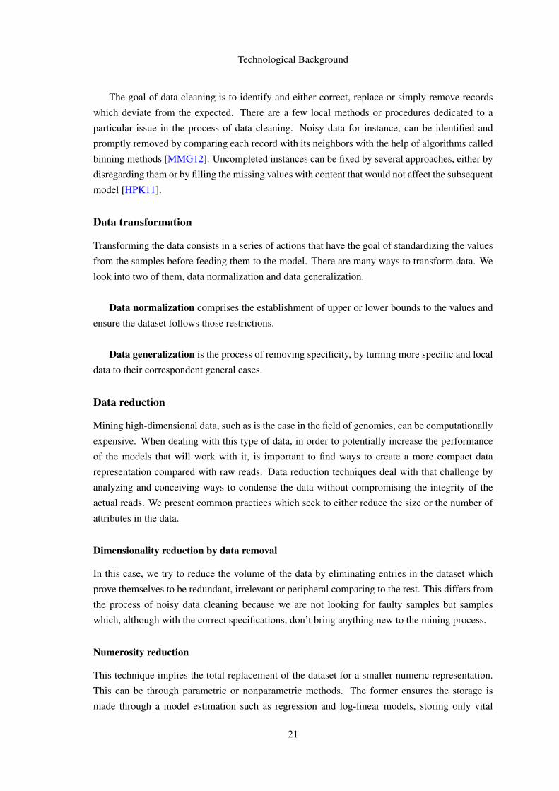


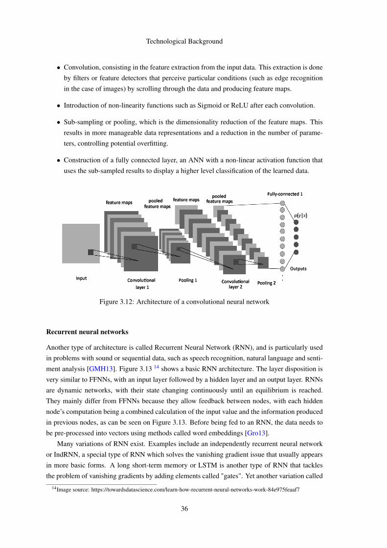


![EIAIcoholismo como una enfermedadEIAIcoholismo como una enfermedad PrOgreSiva ... alcoholismo como unvicio o delito y,en COnSeCuenCia,COmO un ... alcoh61ico・Por e]emplo,el](https://static.documents.pub/doc/80x56/60180c508f72433133531669/eiaicoholismo-como-una-enfermedad-eiaicoholismo-como-una-enfermedad-progresiva-.jpg)


