General enquiries on this form should be made to: Defra, Science Directorate, Management Support and Finance Team, Telephone No. 020 7238 1612 E-mail: [email protected]SID 5 Research Project Final Report SID 5 (2/05) Page 1 of 39
Transcript
General enquiries on this form should be made to:Defra, Science Directorate, Management Support and Finance Team,Telephone No. 020 7238 1612E-mail: [email protected]
SID 5 Research Project Final Report
SID 5 (2/05) Page 1 of 28
NoteIn line with the Freedom of Information Act 2000, Defra aims to place the results of its completed research projects in the public domain wherever possible. The SID 5 (Research Project Final Report) is designed to capture the information on the results and outputs of Defra-funded research in a format that is easily publishable through the Defra website. A SID 5 must be completed for all projects.
A SID 5A form must be completed where a project is paid on a monthly basis or against quarterly invoices. No SID 5A is required where payments are made at milestone points. When a SID 5A is required, no SID 5 form will be accepted without the accompanying SID 5A.
This form is in Word format and the boxes may be expanded or reduced, as appropriate.
ACCESS TO INFORMATIONThe information collected on this form will be stored electronically and may be sent to any part of Defra, or to individual researchers or organisations outside Defra for the purposes of reviewing the project. Defra may also disclose the information to any outside organisation acting as an agent authorised by Defra to process final research reports on its behalf. Defra intends to publish this form on its website, unless there are strong reasons not to, which fully comply with exemptions under the Environmental Information Regulations or the Freedom of Information Act 2000.Defra may be required to release information, including personal data and commercial information, on request under the Environmental Information Regulations or the Freedom of Information Act 2000. However, Defra will not permit any unwarranted breach of confidentiality or act in contravention of its obligations under the Data Protection Act 1998. Defra or its appointed agents may use the name, address or other details on your form to contact you in connection with occasional customer research aimed at improving the processes through which Defra works with its contractors.
Project identification
1. Defra Project code AM0130
2. Project title
An assessment of how process modelling can be used to estimate agricultural ammonia emissions and the efficacy of abatement techniques
3. Contractororganisation(s)
Centre for Ecology and HydrologyBush EstatePenicuikMidlothianEH260QBUK
54. Total Defra project costs £ £149861.00
5. Project: start date................ 01 August 2003
end date................. 31 July 2005
SID 5 (2/05) Page 2 of 28
6. It is Defra’s intention to publish this form. Please confirm your agreement to do so...................................................................................YES NO (a) When preparing SID 5s contractors should bear in mind that Defra intends that they be made public. They
should be written in a clear and concise manner and represent a full account of the research project which someone not closely associated with the project can follow.Defra recognises that in a small minority of cases there may be information, such as intellectual property or commercially confidential data, used in or generated by the research project, which should not be disclosed. In these cases, such information should be detailed in a separate annex (not to be published) so that the SID 5 can be placed in the public domain. Where it is impossible to complete the Final Report without including references to any sensitive or confidential data, the information should be included and section (b) completed. NB: only in exceptional circumstances will Defra expect contractors to give a "No" answer.In all cases, reasons for withholding information must be fully in line with exemptions under the Environmental Information Regulations or the Freedom of Information Act 2000.
(b) If you have answered NO, please explain why the Final report should not be released into public domain
Executive Summary7. The executive summary must not exceed 2 sides in total of A4 and should be understandable to the
intelligent non-scientist. It should cover the main objectives, methods and findings of the research, together with any other significant events and options for new work.
Project Aim1. The aim of this project was to show how mechanistic (process) modelling can be used to estimate
agricultural ammonia (NH3) emissions and assess how such models can be used within the Defra NH3 research programme to improve understanding and quantification of ammonia emissions and the potential for their abatement.
Review of existing models2. A comprehensive review of existing mechanistic models was conducted for the principal
agricultural NH3 sources: livestock housing, manure storage, land application of manures and fertilisers, grazing, cut grasslands and arable crops.
3. The model review highlighted the extent of existing modelling methods and showed where gaps occur in our knowledge of the processes and the types of systems to which these methods have been applied.
4. More specifically, existing housing models tend to be too specialised – focussing on a particularly livestock type or management method (principally slurry-based systems). Manure storage emission models also tend to focus on emissions from slurry whilst no general model of emissions from farm yard manure (FYM) stores exists. Model coverage is significantly better for land-application emissions, but few models exist to simulate NH3 emissions from crops, cut grasslands or grazing.
5. Following the review, a selection of the most useful or accessible models were put through a ‘sensitivity screening’ process to investigate which model parameters or input variables have the greatest influence on the models’ predictions.
6. For the majority of the housing and manure storage models, manure pH was found to be the most influential parameter in the models. This is because the surface pH controls the chemical equilibria at the manure surface and the higher the pH the more NH3 there is available for volatilisation (emission). Other influential parameters and variables were the air temperature and the total ammoniacal nitrogen (TAN) content of slurries and the air flow rate through composting FYM.
7. For the land-application model selected for detailed screening (VOLT’AIR), the soil pH was the most influential parameter with the pH and TAN content of the manure and the soil wetness also
SID 5 (2/05) Page 3 of 28
having a significant influence. Temperature had a smaller influence than expected due to offsetting interactions in the model.
8. For the cut grassland and grazing emission model selected for detailed screening (Pasim), soil pH was also the most influential parameter. The wind speed and ammonium status of the plant were also important.
Testing the models9. A review of results of experiments that determine NH3 emission rates was conducted to provide a
test database, with which selected models could be tested. The VOLT’AIR land-application model was tested with field measurements of NH3 volatilisation from organic manures and mineral fertilisers. On average the model agrees well with the emissions from manures. The model appears to under-estimate the emissions from ammonium nitrate fertilisers but performs well for the other fertiliser types. Unexpectedly, the measurements showed lower emissions from urea than ammonium nitrate, but this difference was consistent with the predictions of the VOLT’AIR model for these runs. Further analysis is required to distinguish the factors (incorporated explicitly in the model), which caused these differences between the experimental results (e.g. meteorology, soil type, application rates etc). It is only through the use of process based models that such differences can be explained.
10. To estimate the range of emissions expected from UK NH3 sources for different climates and farm management methods, a combined model linking slurry storage to land application of slurries was devised and tested using numerous scenarios. These scenarios investigated the effect of manure store dimensions, slurry pH, soil characteristics, manure application timing and climate on the modelled emissions.
11. The slurry storage scenarios predicted the largest emissions for the warmest part of the year, for the stores with the largest surface area and largest slurry pH. The land-application scenarios predicted the largest emissions for dry soils with high pH and of the loam and silt texture classes. The application rate and field dimensions were also important with highest emissions resulting from the largest application rates to the smallest fields. This can be related to an effect where % emissions from large fields are less due to “self-sheltering” (building up a boundary layer), that can only be treated by process models including advection interactions.
12. Methods to reduce the NH3 emissions were included in the scenarios. For slurry storage, the process models demonstrated quantitatively how store covers and surface crusting reduce the ammonia emissions. For the land-application of slurry, the process model (VOLT’AIR) provided robust estimates of the reduction in emissions achieved by incorporating the slurry after application, with the largest abatement benefits shown to occur in the warmest climates. Conversely, the model predicted that slurry application by band-spreading had little benefit to reduce ammonia emissions.
Recapture of ammonia by downwind vegetation13. The recapture of ammonia emissions by downwind farm vegetation is a potential abatement
technique to reduce impacts of ammonia deposition further downwind. Three atmospheric dispersion and deposition models were compared for a range of scenarios to investigate the spatial interactions between sources and nearby vegetation. Although the three models use different approaches, the deposition predictions from them were similar. The differences between the predictions could be explained by the model methodologies used. This shows that the modelling techniques are robust and can be applied in future work to demonstrate the multiple benefits of farm vegetation such as increased atmospheric dispersion, the sheltering of manure stores and abatement of emissions from livestock kept under trees.
Mechanistic modelling for inventories14. Mechanistic modelling has the potential to improve the spatial and temporal distribution of NH3
emissions in the current UK inventory. Currently, the only spatial and temporal variability included in the National Atmospheric Emission Inventory (NAEI) for ammonia is a result of the spatial distribution of livestock numbers, cropping and temporal dynamics of farm management. Conversely, meteorological conditions and soil characteristics are not taken into account which could lead to large errors in the inventory, both spatially and temporally (seasonal differences).
15. To investigate the principle of using mechanistic models to improve inventory estimates, one well-validated emission model, VOLT’AIR, was applied to the English and Welsh grid-squares (10 km) of the NARSES emission inventory model and the emissions from one NH3 source (land-application of cattle slurry) were compared for the two models (VOLT’AIR and NARSES) for two inventory months: January and July.
16. VOLT’AIR gave lower emissions than NARSES for January, while the total emissions were similar
SID 5 (2/05) Page 4 of 28
for July – but with a very different spatial distribution. The proportion of TAN volatilised in the NARSES model is spatially and temporally constant (42% for this source), but varies considerably in the VOLT’AIR process model results due to differences in soil pH and climate. These effects explain the differences between the models and highlight the importance of including process modelling in regional inventories.
17. The comparison between NARSES and VOLT’AIR highlighted the problems of using monthly averaged data (from NARSES) to drive a model that runs at an hourly time-step (VOLT’AIR). This a potential cause of the difference in emissions for January, since, with these input data the runs of VOLT’AIR were made under the assumption of ‘constant drizzle’ (at the average monthly rate), which should be revised in subsequent modelling.
Project conclusions18. This project has shown the potential of mechanistic models to improve our understanding of the
processes and the ability of the models to explain unusual experimental results which would not be possible using empirical models e.g. the prediction of low emissions from urea application. The project has also shown how mechanistic models have the potential to improve the current spatial and temporal distributions of emissions.
19. At present the current gaps in the coverage of existing models mean that a significant proportion of UK emissions (approximately 40%) cannot be modelled mechanistically. The majority of these emissions are from livestock housing; this highlights the lack of general emission models for this source type. Models need to be developed that take into account the air flows and temperature variations within and around different housing types and a better process understanding is needed of pH changes and mixing within slurries. Field models (land application and grassland) can be improved by modifying the routines that handle soil pH and soil water content.
20. To support the mechanistic modelling approaches, experiments need to make accurate measurements of pH (both of the manure and soil) and soil water content since these are the key parameter for many of the models. More accurate meteorological measurements are also needed - particularly farm-yard air flows and temperature distributions. For the modelling of emissions from grazed and cut grassland, accurate measurements of soil pH are also needed. The modelling of grassland systems has stressed the importance of the apoplastic (intercellular) ammonium status of the vegetation for emissions. These parameters are very difficult to measure and more work is needed to refine indicator methods from easier vegetation measurements (e.g. bulk foliar ammonium).
Project Report to Defra8. As a guide this report should be no longer than 20 sides of A4. This report is to provide Defra with
details of the outputs of the research project for internal purposes; to meet the terms of the contract; and to allow Defra to publish details of the outputs to meet Environmental Information Regulation or Freedom of Information obligations. This short report to Defra does not preclude contractors from also seeking to publish a full, formal scientific report/paper in an appropriate scientific or other journal/publication. Indeed, Defra actively encourages such publications as part of the contract terms. The report to Defra should include: the scientific objectives as set out in the contract; the extent to which the objectives set out in the contract have been met; details of methods used and the results obtained, including statistical analysis (if appropriate); a discussion of the results and their reliability; the main implications of the findings; possible future work; and any action resulting from the research (e.g. IP, Knowledge Transfer).
An assessment of how process modelling can be used to estimate agricultural ammonia emissions and the efficacy of
abatement techniquesM.R. Theobald1, A.G. Williams2, J. Rosnoblet3, C. Campbell1, T.R. Cumby2, T.G.M. Demmers2, B. Loubet3, D.J.
Parsons2, B. Gabrielle3, E. Nemitz1, S. Génermont3, E. Le Cadre3, U. Dragosits1, M. Van Oijen1, P. Cellier3 and M.A. Sutton1
SID 5 (2/05) Page 5 of 28
1Centre for Ecology and Hydrology (CEH), Bush Estate, Penicuik, Midlothian, EH26 0QB, UK.2Silsoe Research Institute, Wrest Park, Silsoe, Bedford, MK45 4HS, UK.3Environment and Arable Crops Research Unit (Unité EGC), INRA, Thiverval Grignon, F78850, France.
1. Introductiona. Ammonia emissions and abatement
Emission of ammonia (NH3) from agriculture and its subsequent deposition to sensitive ecosystems imposes a major environmental burden both nationally and internationally. The gradual recognition of this problem has led to NH3 being included in UNECE and EC emissions abatement agreements for the first time, under the Gothenburg Protocol, the National Emissions Ceilings Directive and the Directive on Integrated Pollution Prevention and Control. Many methods for reducing NH3 emissions have been suggested and the potential of several of these have been assessed experimentally. However, it is difficult to assess the potential of abatement nationally due to the variation in climate, soil types and management practices – all of which might modify the effectiveness of a particular technique. The quantification of NH3 emissions in a robust, validated inventory is an essential aspect in measuring the problem and assessing the achievement of environmental targets. The UK NH3 inventory currently contains many values derived from limited experimental data. These may have been measured, for example, from manure of other species of livestock, manure application to one soil or vegetation type, or for limited climatic conditions. In addition, some inventory values are derived from data sets with widely varying values, introducing a substantial uncertainty into the assessment of total emissions.
b. Modelling the system
One way to study the effect of climate, soil type and management practices on NH3 emissions and the potential for their abatement is to use mathematical models. There are many different approaches to mathematical modelling. Two types of model that are used to describe physical systems are empirical models and mechanistic (process) models. The main difference between these approaches is that empirical models use mathematical functions fitted to experimental data whereas mechanistic models represent the individual processes within the system mathematically (although these processes are often parameterised empirically). This distinction is important to make because although there are many empirical models treating NH3 emissions (e.g. MANNER [Chambers et al., 1999], NGAUGE [Brown et al., 2005], FYNE [Theobald et al., 2004) there are far fewer mechanistic models considering NH3. The advantage of the mechanistic modelling approach is that it gives an insight into the individual processes involved and the relationships between them. In principle, mechanistic models should achieve better results than empirical models because they address the key factors that affect emissions, e.g. temperature, moisture content, pH, wind speed, movement of material etc. In addition to this, such models can be broken down into their constituent processes and these can be parameterised and tested separately. This allows a substantial degree of transferability between different systems. The main disadvantages for mechanistic modelling are that the processes must be understood well and this approach results in great complexity. This is in contrast to empirical models which can often be formulated without any knowledge of the underlying processes and, therefore, can be relatively simple and require less detailed input data.
c. Project overview and objectives
This study has reviewed and assessed existing mechanistic models of NH3 emission processes from a variety of agricultural sources. Furthermore, emission abatement scenarios will be assessed by application of these models. An essential stage in the model assessment is a study of the sensitivity of the models to parameter values and input data. This stage is important for two reasons: 1) it highlights which model processes have the largest influence on the resulting NH3 emission and 2) it shows which variables are most important to measure in experimental studies. Once a better understanding of these models has been obtained, it is important to assess how accurately the models can simulate the NH3 emission by comparison with experimental studies. For many of the models this has already been done as part of the model development, but there are datasets remaining that can be used to assess the performance of certain models. The most promising models have been used for scenario analyses to simulate the NH3 emissions (and abatement potential) for an agricultural system under a range of different climatic, soil and management conditions. One model has been combined with the NARSES geo-spatial emissions inventory to demonstrate how such an inventory can be improved using
SID 5 (2/05) Page 6 of 28
mechanistic modelling. The main body of this report presents summaries and overviews of the analysis and modelling and full details are provided in the appendices.
The objectives of the project were:
1. To construct and refine an integrated conceptual framework of nitrogen flows and NH3 emissions to which all process models can be related.
2. To conduct a critical analysis of available NH3 emission process models for agricultural sources.
3. To carry out sensitivity analyses on the process models to identify and prioritise the influence of individual parameters and variables.
4. To construct a database containing data from NH3 emission measurements.
5. To assess the dependence of modelled emission estimates (with and without the application of abatement techniques) on spatially variable parameters such as soil type and climate.
6. To investigate how the modelled emission estimates could be incorporated into the spatial emissions modelling inventory of NARSES.
7. To recommend which process models (or parts therein) are best suited for use within Defra’s ‘Ammonia emissions from agriculture’ research programme.
8. To investigate modelling NH3 recapture by vegetation for different source-receptor configurations.
9. To recommend which variables need to be measured in experiments to enable the results to be best interpreted and used within process models.
2. Modelling ammonia emissions and abatementa. The emission processes
In general, NH3 emissions from agriculture originate at an interface between an NH3-containing aqueous solution and the atmosphere. This is commonly modelled mechanistically using a first order differential equation (Haslam et al, 1924):
dM/dt = A K (PNH3liquid-PNH3air) Eqn 1
The term dM/dt is the rate of NH3 emission in terms of mass per unit time; A is the exposed surface area, K is a mass transfer coefficient (with units of velocity, e.g. m s-1) and PNH3liquid and PNH3air are the partial pressures of NH3 in the bulk of the emitting aqueous solution and in the air above, respectively. is a coefficient that relates the partial pressure of NH3 to the concentration of free NH3 in solution (CNH3liquid), such as the Henry’s Law coefficient, where CNH3liquid = PNH3liquid. The emission process is driven by the difference between PNH3liquid and PNH3air.
When Eqn 1 is applied to different NH3 sources, the terms of the equation can represent many complex processes. A detailed analysis of the application of this equation is presented in Appendix 1.
b. Ammonia emission systems
The main source of NH3 emissions is livestock excreta. There is a flow of N from feed through animals from which useful products are derived (e.g. milk and eggs). Animals excrete N, both in buildings and fields (Figure 1).
SID 5 (2/05) Page 7 of 28
Feed
Animals
N in Excreta
Deposition and short
term storage in buildings
Direct deposition in fields
Ammonia emissions
Storage Land application
Processing ( e.g . separation)
Useful products
Flow of Nitrogen
Flow of NH 3
Figure 1 Simplified framework of nitrogen flows and ammonia emissions from animal production systems. (Shaded boxes represent the focal points of several different process models.)
Nitrogen may be excreted as urea in mammalian urine (or uric acid from poultry) and organic N (Org-N) in faeces. These are mineralised by micro-organisms (mainly bacteria) to liberate ammoniacal N (NH3-N and NH4
+-N, the balance between these depending on pH), with urea being the most bio-degradable and faecal Org-N the least.
Urea hydrolysis is fairly fast, therefore emissions from buildings are relatively large. Emissions continue when manures are stored. Slurries emit a relatively small proportion of ammoniacal N, compared with solid manures. This is because spontaneous composting can raise temperatures considerably (up to about 65°C), greatly accelerating volatilisation, while slurries remain at approximately ambient temperature. After storage, manures are generally applied to land. In conventional application systems, manures are broadcast, so that a large surface area is exposed from which emission can occur. This can be partly mitigated by rapid incorporation or injection (slurry only).
Once on or in land, further mineralisation may occur. The fate of the nitrogen depends on the uptake by plant roots (following nitrification), leaching and uptake by plant leaves. Some N may not follow these routes, leading to ammonia emissions. Plants may also emit ammonia during senescence and can also act as receptors for NH3 deposition.
Mineral fertilisers contain N in three main forms: NO3-N, NH4+-N and urea-N. NO3-N should not
contribute directly to ammonia emissions, although an increase in plant mediated ammonia emission can occur [Sutton et al., 2001]. NH4
+-N will find an equilibrium with NH3-N, depending on the local environment (dominated by soil pH) and ammonia can thus be emitted. Urea-N is in general first hydrolysed to NH3-N/ NH4
+-N before it is taken up by plants or nitrified to NO3—N. Urea tends to
develop a higher pH than ammonium based fertilisers, so leading to generally higher emissions of ammonia.
c. Methods of reducing ammonia emissions
There are many methods available for reducing emissions of NH3 to the atmosphere. When considering the abatement of emissions, it is important to bear in mind the N flow shown in Figure 1 because abatement of NH3 losses in the early stages of the system will result in more ammonia available for emission later [Hutchins et al.,1995]. Another consideration is that some NH3 abatement measures may have the effect of increasing the loss of other pollutants such as N2O and NO3
-; however, this is beyond the scope of this project.
The techniques available to reduce ammonia emissions can be described in the following general terms:
1. Reduce emitting area
2. Reduce pH
3. Reduce air speed over the emitting surface
SID 5 (2/05) Page 8 of 28
4. Increase resistance to mass transfer of the emitting surface
5. Reduce the temperature of the emitting material
6. Reduce rate of mineralisation of organic N to produce TAN
a. Reduce water in poultry litter (to reduce the mineralisation rate of uric acid – does not work for pig or cattle manures)
7. Increase sinks and assimilation of TAN
8. Reduce TAN concentration via dietary manipulation (beyond the scope of current models)
Practical measures to achieve these effects for different NH3 sources are listed in Appendix 2.
d. Canopy recapture models
Following the emission of NH3 into the atmosphere, the gas is readily deposited to vegetation especially semi-natural land and trees [e.g. Sutton et al., 1993]. If this deposition occurs close to the original source on land owned by a farmer then the canopy recapture of the NH3 can be considered an abatement measure since the NH3 is removed from the atmosphere before it has an impact on sensitive conservation areas. Defra project WA0719 ‘AMBER’ (Ammonia Mitigation By Enhanced Recapture) [Defra, 2003; Theobald et al., 2001] investigated the potential of this abatement strategy using a combination of experiments and modelling. In the experiments, NH3 was released upwind of a tree belt stretching 60 m downwind and the proportion of NH3 that was deposited to the leaf and branch surfaces was estimated from measurements. To extend these results to other source-receptor configurations, a 2-dimensional atmospheric dispersion and deposition model was used. This study concluded that tree belts have the potential to recapture 5-10% of the emitted ammonia, while additional benefits include up to 30% reduction in local concentrations (due to additional dispersion) and potentially 30% reduction in emissions due to the sheltering effect of trees, with each of these figures highly dependent on local emission configuration and tree belt design. Lastly, it was expected that agroforestry systems, including animals under trees could reduce net emissions by up to 80%. The current project extends the AMBER modelling to other atmospheric dispersion and deposition models to compare methodologies and predictions. This will provide guidance on which are the most suitable modelling approaches and how these can be applied in future NH3 projects on this emerging research topic.
3. Review of existing modelsa. Review methodology
A literature search was carried out for existing mechanistic NH3 emission models for different source types (livestock housing, manure storage, land application of manures, grazing and fertiliser application). The models were assessed in terms of 16 criteria (Table 1) and the results of these analyses are presented in Appendices 3-7. From these analyses, a decision was made on which models should be assessed further in this project. The same criteria were also used to assess existing canopy recapture models and these analyses are presented in Appendix 8.
SID 5 (2/05) Page 9 of 28
Table 1 Criteria used for evaluation of models
Criteria
1 What is the model for?
2 Processes in common with other models
3 Parameters that need measuring or estimating
4 Limits in application and extrapolation
5 Strengths of parts or whole
6 Weaknesses of parts or whole
7 How mechanistic and empirical it is
8 Ability to deal with abatement processes
9 Potential for use in a geo-spatial national ammonia inventory (e.g. NARSES)
10 Potential to improve the current estimates in the national ammonia inventory
11 Potential for use in national and international ammonia emission and deposition models
12 Level of detail required in input data
13 Availability of suitable input data in terms of variable type together with spatial and temporal resolution
14 Ability to use readily available geo-spatial data (e.g. 30 year meteorological data means, soil textures, vegetation classes on 5 km2 grids)
15 Inclusion of supplementary environmental information (e.g. calculation of nitrate leaching)
16 Usefulness in future experimental work
b. Summary of livestock housing emission models
Six models were assessed (Appendix 3); three were chosen for further analysis:
1. Groot Koerkamp, P.W.G. (1998) Ammonia emission from aviary housing systems for laying hens. PhD Thesis, Wageningen University IBSN 90-5485-885-0 [pp 73-86, Degradation of nitrogenous components and volatilisation of ammonia from litter
Comments This model is useful for calculating NH3 production from litter, concentrating on managerially influenced conditions. However, it does not deal properly with mass transfer to be called a model of NH3 emissions. It is a good research tool, with some potential for abatement. It has a limited capacity for use in inventories, but may show the likely scope of emissions.
2. Monteny, G. J. (2000) Modelling of ammonia emissions from dairy cow houses. Thesis, Wageningen University
Comments This is a mainly mechanistic model, which is very useful for experimental work and for assessing some approaches to abatement. The high level of detail required may mean that it is not suitable for use in inventories.
3. Ni,J.Q., Hendriks,J., Vinckier,C. and Coenegrachts,J. (2000) Development and validation of a dynamic mathematical model of ammonia release in pig house. Environment International 26, 105-115.
Comments This is a useful, largely mechanistic model for mechanically ventilated houses, but it is limited by the need for very detailed data and need to estimate empirical factors for the partition of well mixed and unmixed air. Emissions from a house are also limited to slurry channels, and not floors or
SID 5 (2/05) Page 10 of 28
walls. It makes a good, novel contribution in the effect of CO2 emissions on surface pH. It has potential for abatement processes, but the mathematical solution used seems naïve compared with the description.
c. Summary of manure/dirty water storage emission models
Seven models were assessed (Appendix 4); four were chosen for further analysis:
1. Cronjé A L (2004). Ammonia emissions and pathogen inactivation during controlled composting of pig manure. PhD Thesis, University of Birmingham
Comments This is a largely mechanistic model of composting solid manure, including NH3 emissions. It was designed for in-vessel composting with known air supply, rather than uncontrolled composting of a field heap and so does not represent mainstream practice especially well. Nonetheless, it is the only model to address this major source of NH3 emission.
2. Olesen, J.E. and Sommer, S.G. (1993) Modeling effects of wind-speed and surface cover on ammonia volatilization from stored pig slurry. Atmospheric Environment Part A-General Topics 27, 2567-2574.
Comments This is a largely mechanistic model derived from one for land spreading. The method for calculating the mass transfer coefficient is more suitable and flexible than that used by Muck & Steenhuis (1982) or Ruxton (1995), but there may be some doubts about the details of airflow over and around a store. It has diffusion through layers, but does not address mixing, surface pH effects or generation of NH3 from organic N.
3. Ruxton ,G.D. (1995) Mathematical modelling of ammonia volatilization from slurry stores and its effect on cryptosporidium oocyst viability. Journal of Agricultural Science 124, 55-60.
Comments Based almost entirely on Muck and Steenhuis (1982). Includes microbial generation of NH3 from urea. Uses Haslam’s (1924) relationship for wind speed and temperature on the mass transfer coefficient. Diffusion equation solved by finite difference. Includes NH3 generation from urea, but not other organic N.
4. Scotford, I.M. and Williams, A.G. (2001) Practicalities, costs and effectiveness of a floating plastic cover to reduce ammonia emissions from a pig slurry lagoon. Journal of Agricultural Engineering Research 80, 273-281.
Comments They dealt with the geometry of lagoons as they fill and are subject to evaporation and rainfall and hence produce a changing surface area for emission. Only deals with limited part of NH3 emission process, but useful for inventory work and mechanistic models with non-uniform cross sections.
Four models were thus considered suitable for further examination. Cronjé’s (2004) model was included as being the only one dealing with solid manure, but it was developed for forced ventilation, rather than normal storage. The Ruxton (1995) model was included partly to contrast it with Olesen and Sommer’s (1993) model, but also as obtaining the model code was thought to be easier than the earlier model of Muck and Steenhuis (1982). Scotford and Williams’s (2001) model applied only to the geometry of a lagoon and so was not considered suitable for analysis beyond sensitivity.
d. Summary of land application emission models
The review identified seven mechanistic (m), three part-mechanistic, and seven empirical (e) models (Appendix 5). Of these, two mechanistic and two empirical models were chosen for critical analysis: VOLT’AIR (m), STAL (m), PLÖCHL (e) and ALFAM (e).
SID 5 (2/05) Page 11 of 28
VOLT’AIR [Génermont, 1996, 1997; Le Cadre, 2004]
This model, developed in France, comprises 9 sub-models that simulate the application of organic and mineral fertilisers and the subsequent soil processes and interactions with environmental conditions that result in transfer of NH3 to the atmosphere. The model can operate at an hourly time-step and has the capability to simulate several emissions abatement methods such as timing of application, changing fertiliser characteristics and incorporation of the fertiliser following application.
STAL [Morvan, 1999]
The STAL model, also developed in France, operates in a similar way to VOLT’AIR but some of the processes (such as soil infiltration) are empirically derived rather than mechanistic. This currently limits the application of the model to French acid-loam soils, for which it has been parameterised.
PLÖCHL [Plöchl, 2001]
This model has been empirically derived from 51 experimental datasets of NH3 volatilisation from manure applications using a neural network approach. It can only be applied to situations similar to those from which the parameterisation was derived and therefore is not very suitable for predictions.
ALFAM [Sogaard et al., 2002]
A more complex model than PLOCHL, comprised of 10 empirically sub-models which were parameterised using an EU dataset of emissions from slurry applications. ALFAM is able to simulate abatement measures such as the timing of the application, changing the slurry characteristics, incorporation, band spreading and injection techniques.
e. Summary of grazing and fertilizer/vegetation emission models
NH3 volatilisation from grazed systems has been modelled by soil-plant process models such as DN-DC [Li et al., 1992] and CENTURY [Parton et al., 1987]. However, the NH3 components of these models are very simplified and mainly focus on chemical equilibria within the soils and the resulting volatilisation. Neither of these two models simulate the bidirectional exchange of NH3 between the plant and the atmosphere, which is an important component of the flux for both intensively and non-intensively managed grassland [e.g. Milford et al., 2001]. One carbon-nitrogen simulation process model that has been modified specifically to model the bidirectional flows of NH3/NH4
+ is Pasim [Riedo et al., 2002] which is based on the Hurley Pasture Model [Thornley, 1998]. Pasim is assessed in detail in Appendix 6;a brief summary follows:
Model use: Models carbon (C), nitrogen (N) and energy dynamics of productive pastures taking into account pasture management, fertiliser application and grazing. Developed by modifying an existing grassland process model by combining it with a resistance model of gaseous NH3 exchange. The model operates at an hourly time step and simulations can be run for time periods of a few hours to decades.
Input variables: Large number including meteorological variables (hourly values), soil variables, grassland initial conditions (C, N concentrations etc.) and management data (livestock numbers, fertiliser application, cutting etc.).
Strengths: Pasim can simulate the bi-directional exchange of NH3 between plant and atmosphere and can also simulate the nitrogen status of the plant.
Weaknesses: With present parameterisation, peak NH3 emissions after cutting and fertilisation may be underestimated and the overall emission of N2O is also underestimated.
Conclusions: Pasim is a useful tool for simulating the nutrient dynamics of individual managed grasslands including the NH3 exchange with the atmosphere. It is also useful for developing relationships between emissions and other factors such as climate, management and abatement techniques. Due to the need for detailed meteorological, soil and management data, the modelling approach of Pasim is not suitable for general application e.g. as part of a national inventory, but the trends of the model output could be used for this purpose. For this reason, and the fact that it is the only grazing model that can simulate bi-directional exchange, Pasim was chosen for further analysis.
SID 5 (2/05) Page 12 of 28
4. Sensitivity screening of the modelsa. Sensitivity analysis vs. sensitivity screening
To understand fully the behaviour of a complex mathematical model, it is usually necessary to carry-out a sensitivity analysis to investigate the model’s response to variations in the values of the model parameters and variables. This is necessary because it is important to know which parameters and variables have a strong influence on the model output and therefore need to be accurately parameterised or measured. Descriptions of mathematical models routinely use the terms ‘parameters’ and ‘variables’ but there are no strict definitions of these terms. For the following analyses we will use the following definitions:
Parameter: Entity that is considered to be constant at a specific location e.g. soil pH, dry matter content of manure
Variable: Entity that is considered variable at a specific location e.g. wind speed, air temperature, rainfall.
Sensitivity analysis (SA) generally proceeds in five steps [Saltelli et al., 2000] (1) quantifying the probability distributions of variables and parameters; (2) selecting representative sets of variable and parameter values from the probability distributions; (3) running the models for the selected sets; (4) quantifying the resulting overall output uncertainty; (5) quantifying the contribution of the different variables and parameters to output uncertainty.
For the current project it was not possible to carry out a detailed SA for every model assessed because there are too many of them. Instead a ‘sensitivity screening’ was performed which allowed assessment of the sensitivity of all the models to the majority of parameters and variables. The protocol for this assessment is listed in Appendix 9. This protocol generates a ‘sensitivity value’ (S) for each parameter and variable assessed; larger values signifying greater influence on the model output.
b. Sensitivity screening of housing and storage emission models
The sensitivity screening for housing and storage emission models is presented in full in Appendix 10. Table 2 to 5 give the summary values of the sensitivity value (S) for each parameter or variable assessed for each of the models in order of decreasing influence on the model output.
Table 2 Sensitivity screening for poultry litter degradation in laying hen house (Groot Koerkamp, 1998)
Table 3 Sensitivity screening for composting pig farmyard manure (FYM) (Cronjé, 2004). Mass of TS is a parameter relating to the degradability of the substrate
Parameter (P) or Variable (V)
Mean sensitivity value (S)
Ranking
Air flow rate (P) 0.39 1Initial moisture content (P) 0.15 2Initial C:N ratio (P) 0.13 3Saturation of off gas (P) 0.070 4Mass of TS at equilibrium (P) 0.045 5Ambient air temperature (V) 0.019 6Initial TAN: Org-N ratio (P) 0.007 7Initial pH (P) 0.001 8
SID 5 (2/05) Page 13 of 28
Table 4 Sensitivity screening for slurry storage model - Olesen and Sommer (1993)
Parameter (P) or Variable (V)Parameter/Variable
values usedMean sensitivity value (S) after time t, days
Table 5 Sensitivity of lagoon geometry in terms of the coefficient of variation (CV) of surface area - Scotford and Williams (2001)
Parameter Mean sensitivity value (S) Ranking
Max depth 0.44 1Base length 0.30 2
Rise angle () 0.23 3
c. Sensitivity screening of VOLT’AIR land spreading emission model
Details of the sensitivity screening for the VOLT’AIR model are listed in Appendix 11 and a brief summary of the method and results follows:
Two parameter groups (slurry properties and soil properties) and one variable group (meteorological variables) were identified for the screening. Two separate analyses were carried out: 1) independent runs for different parameter/variable values whilst keeping all other parameters/variables at median values (i.e. no analysis of interactions between parameters/variables) and 2) combined runs using all possible combinations of parameter/variable values. Table 6 shows a comparison between the sensitivity values for cumulative NH3 emission after 15 days of the independent and combined screening runs.
Table 6 Sensitivity screening of cumulative NH3 emissions of the VOLT’AIR model. The shaded rows indicate the 8 most influential parameters and variables for the combined runs.
* The sensitivity values above 100 or with a division by zero were deleted (number in parenthesis). These result from model runs using parameters at the limits of their ranges.** Ksat is the soil hydraulic conductivity at saturation, b is a parameter in Campbell's hydraulic conductivity equation [Campbell, 1974] and Hsat is the water suction at air entry value. When the water content at saturation is lower than the initial water content, the latter took the value at saturation.
Both the independent and combined runs give the soil pH as the most influential parameter. The sensitivity value (S) for the combined runs is significantly larger than that from the independent runs suggesting that the emissions are sensitive to interactions between soil pH and other soil parameters; this also seems to be the case for the initial soil water content and Campbell’s Ksat (soil hydraulic conductivity at saturation). Out of the slurry parameters, ammoniacal nitrogen content and slurry pH are the most influential. Similar values of S (for the slurry parameters) for the independent and combined runs suggest that interactions between slurry properties are not significant. Out of the meteorological variables studied, wind speed and water vapour pressure are the most influential. Interactions between these also do not seem to be significant.
d. Sensitivity screening of Pasim grassland model
The emission (or deposition) flux calculated by the Pasim grazing model has 3 components: soil flux, stomatal flux (plant-atmosphere exchange through the leaf stomata) and cuticular flux (deposition to the leaf surface). Appendix 13 presents the results of the sensitivity screening in full. Table 7 below lists the parameters, management and meteorological variables to which the simulated total annual ammonia flux is most sensitive.
Table 7 Sensitivity screening results for the Pasim model for total NH3 flux
Parameter Mean sensitivity value (S) Meteorological variable Mean sensitivity value (S)
Soil pH 0.93 Windspeed 0.60
SID 5 (2/05) Page 15 of 28
Min fraction of NH4+ in apoplastic N 0.50 Water vapour pressure 0.35
Thickness of soil layers 0.36 Total solar radiation 0.33
Saturated soil water content in surface layer 0.35 Air temperature 0.18
Minimum cuticular resistance 0.23 Rainfall 0.08
Fraction of leaf water in apoplast 0.22 Management Parameter Mean sensitivity value (S)
Shoot fresh to dry biomass ratio 0.21 Livestock Density 0.13
Apoplastic pH 0.19 Duration of grazing 0.11
Cuticular resistance factor b 0.15 Grazing start date 0.10
Soil pH is the most influential parameter on the simulated total ammonia flux. This is due to the control exerted on the soil ammonia flux by soil pH. The soil layer thickness and the saturation soil water content of the surface layer also have high sensitivity values, however, this is due to a threshold effect; above a critical value these values have very little impact on the simulated total ammonia flux.
The parameters listed in table 7 which are associated with the stomatal flux are the minimum fraction of ammonium in the apoplastic nitrogen content, the fraction of leaf water in the apoplast, the shoot fresh to dry biomass ratio and the apoplastic pH. The parameters associated with the cuticular flux are the minimum cuticular resistance and the cuticular resistance factor b. With the exception of the fresh to dry biomass ratio, all of these parameters are exceedingly difficult to measure and have significant small scale spatial variability. However, the sensitivity of the total flux to these parameters justifies research effort in order to characterise empirical relationships between these parameters and standard simple measurements of vegetation properties.
The sensitivity of the modelled total ammonia flux to meteorological variables was evaluated at four UK sites (see Appendix 13 for details). The results presented in Table 7 are the means of the sensitivity values for each variable. The wind speed has the highest mean sensitivity value, followed by vapour pressure, solar radiation and air temperature, then finally rainfall. The rainfall does not exert a strong influence at any of the four sites. Thus, to reduce the uncertainty in simulated total ammonia flux, it would be most effective to address errors in the wind speed, vapour pressure and solar radiation measurement data.
The sensitivity to grazing management was assessed for the livestock density, the duration of grazing and the start date of the grazing period. It was found that the sensitivity value of each of the grazing management parameters was relatively low, thus small changes in these data will have a relatively small effect on the simulated total annual ammonia flux.
5. Comparison of measured and modelled emissionsa. Data suitable for testing of emission models
Appendix 14 lists datasets that are available for testing NH3 emission models including those that have been used in this project to validate existing models.
b. Testing the VOLT’AIR land spreading emission model
VOLT’AIR has been tested using experimental emission data from the 4 experiments listed in Appendix 14. Most of the measurements were made over 7-day periods. The results of the two farmyard manure (FYM) applications are not yet published. Figures 2 and 3 show the comparison between measured and modelled cumulative ammonia volatilisation, 7 days after application, for organic and mineral fertilisers. Each point represents one single fertiliser application. Most of the points are included within a 50% error limit. FYM and UAN solution give the best fit between measurements and the model. We also notice that urea gives a negligible volatilisation. We may thus consider that the mixture of AN and urea prills (pellets) can be considered as simple AN prills. The AN prills points are widely distributed, but if we consider the mean of the 4 points, measurements and model results are similar. Modelled and measured emissions from urea were lowest out of all fertilisers. This is the opposite to studies in the literature which generally give the highest emissions from urea. The fact that the model agrees with the experimental emissions suggests that the mechanistic modelling approach can provide an explanation for the low urea emissions. However, more analysis is needed to reveal which model
SID 5 (2/05) Page 16 of 28
inputs (e.g. soil type, soil pH, wetness, and meteorology) can explain this behaviour. Finally, although VOLT’AIR was not calibrated with these results, simulated and measured volatilisation fit reasonably well.
Figure 2 Comparison of modelled and measured cumulative volatilisation for different manure applications using the VOLT’AIR model [Génermont, 1996, 1997; Le Cadre, 2004] and measurements (slurry) of Génermont (1996) and unpublished data (FYM).
Figure 3 Comparison of modelled (VOLT’AIR model) and measured [Le Cadre, 2004] cumulative volatilisation for different fertiliser applications.
6. Scenario modellinga. Using scenarios to predict farm-scale ammonia emissions
SID 5 (2/05) Page 17 of 28
As highlighted in Section two, NH3 emissions are an integral part of agricultural N flow. If suitable and reliable models existed for each NH3 source, it would be possible to construct a farm emission modelling framework that could simulate emissions from all farm activities. This framework could then be tested with a range of input data (environmental conditions, different management strategies, different methods of abatement etc.) to study how total farm emissions respond and can be controlled. The review of existing models in Section three shows that suitable models are not available for all source types and therefore a simpler system has had to be constructed consisting of manure storage and land application. The lack of suitable housing emission models means that this significant source type has been omitted from the analysis.
b. Manure storage scenarios
A full description of the scenarios used is given in Appendix 15. A summary follows:
Scenarios were developed for a dairy cattle and finishing pig unit. These operations were chosen because suitable models exist for the storage and spreading of cattle and pig manure. The pig unit was simpler, with a fixed stocking rate, while the dairy farm had variable stocking, with most (at times, all) animals at grass in the summer and hence less excreta collected in the housing and milking area. The pig and dairy units had roughly equivalent numbers of livestock units. Excreta production and wash water used were based on values derived from RB209 [Defra, 2000] for different classes of livestock. With dairy cows at grass, it was assumed that they spent 2 h per day in housing during milking. This proportion of excreta production was thus included in the output from the housing.
It was also assumed that some rainwater entered the slurry system and that all slurry entered one system, i.e. there was no separate dirty water handling. Some rain water evaporates between its precipitation and arrival a slurry tank. This was set to an arbitrary 15%. Once the diluted slurry arrived in the store, it was assumed that rainfall entered the store according to its surface area. Evaporation was set at 80% of that calculated by the Penman formula for evaporation over an open surface of water [ES0117 ‘SCENTS’ final report to Defra, 2005]. It was assumed that all slurry stores would be emptied three times a year: in February, July and November. The store was cylindrical and could be of five heights: 1.2, 2.4, 3.6, 4.8 and 6 m depending on expected rainfall in the location. The slurry pH values were the mean of those measured in the SCENTS small scale experiments.
There is no mechanistic model for ammonia losses from accumulating FYM. Consequently, emission estimates were taken from ADAS’s MANNER program [Chambers et al., 1999]. The pH values were provided by David Chadwick (Pers comm., Head of Wastes Group at IGER).
Four abatement options for storage ammonia emissions were modelled: 1) reduction in slurry pH, 2) reduction in surface area, 3) covering the slurry stores and 4) crusting of the slurry surface.
c. Land spreading scenarios
A full description of the scenarios used is in Appendix 16 with an additional description of the soil data used in Appendix 17. A brief summary of the scenarios follows:
Data from the manure storage scenarios (e.g. TAN content, pH) were passed to the land spreading scenarios which included variations in soil type, application dates, manure types and inorganic fertiliser types. These scenarios also studied the effect of different abatement methods such as band spreading and incorporation after different time periods since application.
d. Meteorological scenarios
The manure storage and land spreading scenarios were analysed under a range of meteorological data taken from 3 sites in the UK. The meteorological data were taken from the Environmental Change Network sites [ECN, 2005] at Drayton, North Wyke and Rothamsted. It was hoped to obtain data reflecting the whole range of UK meteorological conditions but it was not possible to obtain data of a sufficient quality for a site in the north of the UK. To allow analysis over a wide a range of conditions as possible, extreme years out of all sites (warmest, coolest, wettest and driest) were selected as well the average years. The full analyses of these datasets are in Appendix 18.
e. Summary of manure storage results
The full results of the analysis are listed in Appendix 19.
With a tank height of 3.6 m, the results showed that there were relatively small differences in ammonia emissions between locations (different meteorological conditions). The weather affected not only N
SID 5 (2/05) Page 18 of 28
losses, but also straight dilution of the slurries with rainwater so that the TAN and Org-N concentrations were 16% higher in the driest year than the average North Wyke scenario. The overall effects of weather are complex, as are the interactions between the measured variables.
The distribution of emissions within the year was not uniform, with relatively more ammonia emitted from the July-November accumulation period and much less from the November-February period. There were differences between the weather scenarios, with the biggest being in the November-February period with both the driest and coldest scenarios giving less emission than that of the milder North Wyke. Of course, although milder, the winter weather in North Wyke is windier, which also enhances the ammonia emission rate.
Increasing the store depth (h) reduces the exposed area per unit volume (SA/V) stored and therefore represents an abatement option. Figure 4 shows the combined effects of changing the store depth and changing the slurry pH. Generally total NH3 losses are lower for deeper stores and more acidic (lower pH) conditions. For the higher pH values, the total loss of N is linear with 1/height but becomes non-linear at pH values greater than 7.5. Similar scenarios run with the North Wyke meteorological data show that modelled NH3 emissions are 8% greater at North Wyke compared with Rothamsted.
Lowering pH from 7.5 by a unit to 6.5 cut emissions by nearly 90%, while allowing it to increase to 8.5 exacerbated emissions over five fold. The effect was also examined using North Wyke meteorology and the results were almost identical - the effect of pH can be considered universal.
Two other abatement techniques: covering slurry stores and surface crusting are investigated in Appendix 19.
0
10
20
30
40
50
0.15 0.25 0.35 0.45 0.55 0.65 0.75 0.85 Surface area / volume (1/h), m -1
Los
s of t
otal
N, %
pH 6.5 pH 7 pH 7.5 pH 8 pH 8.5
Figure 4 Effect of changing slurry store surface area to volume ratio (SA/V) and slurry pH on the loss of ammonia for a pig slurry store using Rothamsted meteorological data.
f. Summary of land spreading results
The full results of the scenarios without abatement measures are listed in Appendix 20.
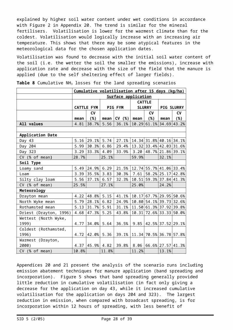
Cumulative NH3 volatilisation 15 days after manure spreading is given in Table 8.
The cumulative volatilisation is similar for cattle and pig FYM. Volatilisation is higher for pig slurry than for cattle slurry, due to the higher ammoniacal nitrogen content of the pig slurry. Volatilisation seems quite low for FYM.
The application date has a large influence on the cumulative losses with a coefficient of variation (CV) of c. 25 to 60%. This variation is due to the different time periods of meteorological data used (e.g. air temperatures and wind speeds).
SID 5 (2/05) Page 19 of 28
Volatilisation is also affected by the soil type, giving a CV of c. 24 to 27 % of the mean volatilisation from manures. The soil type has much less influence with mineral fertilisers (Appendix 20). Appendix 20 also has a more detailed analysis of the effect of soil type. This analysis shows that the most influential parameter is soil pH (in agreement with the sensitivity screening) and if the same (median) soil pH is used for each soil type then soil texture is most influential with finer soils giving less volatilisation.
The meteorological scenario has the least influence for manures, with a CV of c. 11 to 13% only. The influence for mineral fertilisers is higher, with a CV of about 22 to 95 %. The mean volatilisation for manures is generally lower under the wettest meteorology than under the driest. This may be explained by higher soil water content under wet conditions in accordance with Figure 2 in Appendix 20. The trend is similar for the mineral fertilisers. Volatilisation is lower for the warmest climate than for the coldest. Volatilisation would logically increase with an increasing air temperature. This shows that there may be some atypical features in the meteorological data for the chosen application dates.
Volatilisation was found to decrease with the initial soil water content of the soil (i.e. the wetter the soil the smaller the emissions), increase with application rate and decrease with the size of the field that the manure is applied (due to the self sheltering effect of larger fields).
Table 8 Cumulative NH3 losses for the land spreading scenarios
Cumulative volatilisation after 15 days (kg/ha)Surface application
CATTLE FYM PIG FYMCATTLE SLURRY PIG SLURRY
mean CV (%) mean CV (%) mean CV (%) mean CV (%)All values 4.81 38.7% 5.56 36.1% 10.29 61.1% 34.69 43.2%
Appendices 20 and 21 present the analysis of the scenario runs including emission abatement techniques for manure application (band spreading and incorporation). Figure 5 shows that band spreading generally provided little reduction in cumulative volatilisation (in fact only giving a decrease for the application on day 43, while it increased cumulative volatilisation for the application on days 204 and 323). The largest reduction in emission, when compared with broadcast spreading, is for incorporation within 12 hours of spreading, with less benefit of incorporation after 24 hours. Manure incorporation seven days after application only reduced emissions for the application on day 43 and actually increased emissions for the applications on days 204 and 323. Further analysis is needed to explain some of these interactions.
SID 5 (2/05) Page 20 of 28
0
2
4
6
8
10
12
14
16
BROADCAST BAND INCORP 12h INCORP 24h INCORP 7d
Cum
ulat
ive
vola
tilis
atio
n af
ter 1
5 da
ys
(kg
N /h
a)
Day 43 Day 204 Day 323
Figure 5 Effect of different abatement techniques (band spreading and incorporation after 12 hours, 24 hours and 7 days) on the cumulative NH3 losses for the 3 different application dates modelled using VOLT’AIR (mean values taken from all combined model runs).
From all of the scenario model runs, the mean volatilisation abatement is about 7% for band spreading and 43-49 % for incorporation 12 hours and 24 hours after spreading. The mean abatement is negligible when incorporation is made after 7 days.
The analysis in Appendix 20 also investigates the effect of extent and depth that the manure is incorporated (volatilisation decreasing both with extent and depth).
7. Use of process models in national inventoriesa. Emission inventory approaches
Inventories of gaseous emissions are used at local, regional and national scales to provide an overview of the contribution of different sources to the total emission as well as provide input data for atmospheric dispersion models. The total emission from the inventory can also be used to compare with statutory emissions targets to assess compliance. Emissions can vary spatially and temporally and ideally inventories should capture this variation although simplifications have to be made. For NH3 emissions in the UK, the inventory prepared by Misselbrook et al. (2000) has been used by Defra to provide an estimate of total UK NH3 emissions which can be compared with the 2010 emissions target of 297 kt per year set under the National Emission Ceilings Directive and the Gothenburg protocol. The ammonia terms in the National Atmospheric Emissions Inventory (NAEI) thus use an ‘emission factor’ approach i.e. the NH3 emissions are estimated by applying a factor (e.g. g NH3-N animal-1 day-1) estimated from experimental studies. Emission estimates are calculated for the main stages of agricultural management: livestock housing, grazing, storage and land-application of manure and slurry and fertiliser application. These are further subdivided into the main livestock classes: cattle (9 sub-classes), pigs (7), poultry (5), sheep (2), goats (2), horses (1) and deer (3). Despite this detailed breakdown of emissions, the inventory provides no information regarding their spatial and temporal variability. Estimates of the UK spatial variability of ammonia emissions are provided for the NAEI using the AENEID model (Ammonia Emissions for National Environmental Impacts Determination, Dragosits et al. 1998, Dragosits and Sutton 2004). The maps produced have the advantage of linking parish agricultural statistics directly with 1 km resolution land cover data, but the direct coupling to the NAEI totals means that the spatial effects of meteorology, soils etc are not incorporated.
b. Description of NARSES emission inventory
Under the Defra-funded project ‘NARSES’ (National Ammonia Reduction Strategy Evaluation System) – AM0101, a new NH3 emission inventory has been produced which does provide the potential to include some spatial and temporal variability. As well as being an emission inventory, NARSES also incorporates NH3 emission abatement techniques and their costs and can therefore be used to explore
SID 5 (2/05) Page 21 of 28
emission reduction scenarios. It calculates cost curves to give the costs necessary to implement these scenarios. The NARSES inventory takes a slightly different approach to that used by Misselbrook et al and uses the concept of total ammoniacal nitrogen (TAN) flow. TAN is the nitrogen that is in the form of both NH3 and NH4
+ and is present in slurries and manures produced by livestock. The NH3 emission from a particular source will be derived from the TAN pool of that source and therefore an emission factor can be derived from experiments giving the proportion of TAN present that is emitted as NH3. The focus of NARSES is to allow calculation of abatement and costs, as well as, in future, the effects of soil and climatic variation at a low spatial resolution (10 km) using non-disclosive datasets. The approach of NARSES therefore complements the fine scale spatial variability assessment of the AENEID model, therefore progress has also been made in refining a coupled NARSES-AENEID approach. This combines the potential for spatial variability in abatement options of NARSES (10 km) with the fine scale effects of land cover, including disclosive datasets at 1 km of the AENEID approach, for application in atmospheric transport models. Appendix 22 provides more details of the emissions modelling methodology used in NARSES.
c. Feasibility of including process models into a national inventory – VOLT’AIR
To assess how the NARSES emission inventory could be improved by the inclusion of process-based models, the land-application model VOLT’AIR was applied to each NARSES 10 km grid-square. This model was chosen because it is a well-validated model with a short run-time and so can be applied to all 3000 10 km grid-squares within a reasonable time period. The objective of this assessment was to determine if the data used in NARSES are sufficient to drive the VOLT’AIR model and if so how does the emission estimate and also the spatial and temporal variability of the emissions differ between the two approaches. Full details of this assessment are presented in Appendix 22; a summary of the analysis follows:
The first step was to prepare VOLT’AIR input data that correspond to the data available to the NARSES model. The English and Welsh soil data that NARSES uses come from the National Soil Resources Institute (www.silsoe.cranfield.ac.uk/ nsri / ) and the meteorology data come from the UK climate impact programme (UKCIP) (http://www.metoffice.com/research/hadleycentre/obsdata/ukcip/). Soil data for Scotland were not available to this project and therefore the analysis was restricted to England and Wales. The soil and meteorological data are at a grid resolution of 5 km and were averaged to 10 km to match the grid resolution of NARSES. Meteorological data from January and July were used to investigate the temporal variations of the emissions. VOLT’AIR runs at an hourly time-step but since only monthly meteorological data are available to NARSES, VOLT’AIR was run on the mean monthly values.
One emission source was investigated: the emissions from cattle slurry applied to arable land. This source was chosen because it is a widespread practice throughout the UK and the emission process is well characterised in VOLT’AIR. The baseline NARSES model was run and the mass of TAN applied to each grid square (in the form of cattle slurry to arable land) was used as input to VOLT’AIR. Figure 6 shows a comparison of the NH3 emission per grid-square for VOLT’AIR and NARSES for January and July.
Figure 6 A comparison of the grid-square emissions of VOLT’AIR and NARSES for the two months January and July.
On average, VOLT’AIR gave lower NH3 emissions per grid-square than NARSES and this was more pronounced in January where VOLT’AIR gave lower emissions for the vast majority of grid-squares. These differences are the result of different % NH3 volatilisation rates. In NARSES, the % volatilisation of TAN is fixed at 42% but for the VOLT’AIR results it ranges from 0-84%. The most influential factor determining the % volatilisation of VOLT’AIR is the soil pH (Figure 7) with volatilisation increasing with pH. Other important factors are: hours of sunshine and rainfall (for January) and air temperature and rainfall (for July).
Abatement was modelled in VOLT’AIR using the same scenario as the NARSES baseline (12% incorporation of slurry after 24 hours and 1% injection of slurry for all grid-squares). For January VOLT’AIR estimated a reduction in emissions for incorporated slurry (compared with surface-spread) of about 50% whilst for July the reduction was about 43%. Emissions from injected slurry were assumed to be zero because VOLT’AIR cannot presently model this method of application.
Figure 7 Plot showing the dependence of the % volatilisation from the VOLT’AIR model on soil pH for January and July
8. Modelling canopy recapturea. Existing models
Appendix 8 contains a full review of existing canopy recapture models and approaches using the assessment criteria of section 3. A summary of three most useful models follows:
MODDAAS 2D: The MODAAS-2D [Loubet, 2000] model derives from the coupling of a Lagrangian Stochastic (LS) dispersion model with a leaf-scale ammonia exchange model. It is a steady state, two-dimensional model, with no chemical interactions. The model simulates the dispersion of ‘particles’ (i.e. NH3 molecules) from the source as they travel through the canopy. The interaction (i.e. bi-directional exchange) with the canopy is handled by the NH3-exchange sub-model. By simulating a large number of particle trajectories, a concentration and deposition field can be built-up. Disadvantages of this model are primarily the long run-time and the steady-state output.
FIDES-2D: The FIDES-2D [Loubet et al, 2001] model uses an analytical solution to the standard diffusion equations to simulate the concentration and atmosphere-canopy exchange of NH3 downwind of a source. In a similar way to MODDAAS-2D, FIDES-2D models the canopy interactions using a leaf-scale NH3 exchange model. Due to the fast model run-time it is possible to use a time-series as input data, thus producing a pseudo-variable-state model to simulate temporal changes in the dispersion and canopy exchange. The main disadvantage of this model is that it does not model the dispersion and exchange of NH3 within the canopy, just at the canopy surface.
SID 5 (2/05) Page 23 of 28
LADD: LADD [Hill, 1998] is a 3-dimensional dispersion and deposition model. It is a Lagrangian model that simulates the dispersion and deposition of NH3 by moving a vertical column of air along straight-line trajectories across a grid. As the column moves across the grid, NH3 is emitted into the lowest layer from sources along its trajectory and mixed vertically within the column at a rate determined by the turbulent diffusion coefficient (K). Deposition from the lowest layer to the surface is dependent on the land use assigned to the grid-square. The measured wind direction frequencies (for each 10° sector) are used by the model to weight the contribution, to concentrations, from each trajectory. Since LADD is a 3-dimensional model, the run times can be long. Other disadvantages are that bi-directional exchange with the surface is not simulated and (like FIDES-2D) within-canopy dispersion is not modeled.
b. Modelling recapture scenarios
Within the Defra project AMBER [Defra, 2003], the MODDAAS-2D atmospheric dispersion and deposition model was used to simulate a range of source-receptor configurations i.e. spatial relationships between NH3 emission sources and nearby vegetation. Two groups of scenarios were analysed: 1) canopy recapture of emissions from livestock housing/manure storage and 2) canopy recapture from emissions from land spreading of manures. A full list of the scenarios can be found in Appendix 23. The current project takes the same scenarios and re-simulates them using the LADD and FIDES ammonia dispersion and deposition models to compare the 3 different approaches to modelling canopy recapture.
c. Recapture scenario results
The comparison of the canopy recapture simulated by the 3 models (Appendix 23) shows that the LADD and FIDES-2D models give very similar predictions. The main differences between their predictions are due to the wind speed being constant with height in the LADD model or are due to different ways that the scenarios have had to be represented in the two models. The MODDAAS-2D model generally gave lower recapture rates which can be explained by the way the canopy structure is represented in the model. In this model application, the canopy structure was very open at low levels and therefore much of the NH3 passed through the lower levels of the canopy without being recaptured. Changing the canopy structure in the model had a large effect on the amount of NH3 recaptured, which demonstrates that a complex dispersion model is required to take into account variations between different canopies.
9. Priorities for future modelling and experimental worka. Priorities for future model development
Appendix 28 suggests priorities for future development of mechanistic NH3 emission models as a result of the analyses of this project. A brief summary follows:
Housing and storage emissions modelsWe recommend that improvements in modelling of slurries should concentrate on:
1. Prediction of surface pH as affected by bulk pH changes, CO2 emission and mixing by wind and thermal effects
2. Prediction of surface resistance changes as crusts are generated and destroyed.
3. Better prediction of Org-N degradation in slurries
4. Expansion of implementation to deal with weeping wall stores and flushed slurry channels
5. Modelling of air flows within naturally and mechanically ventilated houses
6. Spatial temperature effects in houses
Land-application model and grassland model (VOLT’AIR and Pasim)Two important factors for both of these models are the soil pH and the soil water content and there is potential for improvement of the routines that use these parameters. Improvements specific to VOLT’AIR include modelling applications made in presence of a crop canopy, modelling slurry application by injection (which is currently assumed to give zero emissions in the model), improving the
SID 5 (2/05) Page 24 of 28
infiltration routine of the model, and modelling the evolution of manure characteristics (e.g. crusting). Specific Pasim improvements include the incorporation of routines to model interactions between canopy resistances, the difference between root uptake of ammonium and nitrate and decomposition above the soil surface.
b. Priorities for future experimental work
Appendix 28 suggests priorities for future experimental work as a result of the analyses of this project. A brief summary follows:
1. pH measurements - The sensitivity analyses for stored slurry highlight the importance of surface pH. In most experimental work, bulk pH is measured. There is great need to measure surface pH as well and to high degree of accuracy. Soil pH is a key factor for the VOLT’AIR and Pasim models and therefore should be measured accurately.
2. Soil water content - The VOLT’AIR and Pasim models would be improved by incorporating better soil water content routines. These model improvements would necessarily need to be backed-up by accurate soil water measurements.
3. Organic matter degradation - As organic matter degrades, it can influence ammonia emissions in two ways: 1) mineralisation of organic-N thereby increasing the source strength and 2) heat generation in solid manures. Improved characterisation requires more experimental work, but should be conducted in conjunction with modellers.
4. Meteorology - Sometimes, wind speeds are measured at only one height, so that assumptions have to be made about wind profiles. Measurements at, at least, two heights are required. Animal houses are complex structures and detailed characterisation of internal air speeds (and their connection with the external environment) is needed to enable a mechanistic model to operate successfully. To reduce uncertainties in the model predictions of VOLT’AIR and Pasim, it is recommended that wind speed, vapour pressure and solar radiation data are measured as accurately as possible.
The cost of erroneous measurements may be incalculable. If possible, three sensors should always be used for each measurement.
10. Discussiona. Key findings of this project
This project has highlighted three main points concerning the use of mechanistic models to simulate ammonia emissions:
1. Many different models exist of varying complexity but there are still significant gaps in the range of systems that can be modelled (the model coverage).
2. Sensitivity screening of a range of mechanistic models has shown that the parameters and variables that a model is most sensitive to depends on the processes modelled and how they are represented. However, the analysis has also shown that certain parameters and variables have a strong influence on a range of models e.g. pH.
3. The application of a single model to the full range of conditions in England and Wales gives a large range of emission estimates highlighting the potential spatial and temporal variability of NH3 emissions.
b. Model coverage
In this section values for UK emissions are taken from the NH3 emission inventory of Misselbrook et al (2000). In Section 3, six models of housing emissions were assessed. Three of these were considered not useful because they are either too simple or model processes in a way that is not appropriate to calculate emissions. The three remaining models estimate emissions from quite specialised systems, hence leaving gaps in the coverage of housing systems. From Table 2 in Appendix 3, significant gaps can be seen for pig housing on FYM, poultry housing and cattle housing on FYM. From the emission inventory, these gaps represent 21% of UK NH3 emissions. The situation is similar for the manure and slurry storage emission models (see Table 2 in Appendix 4) with gaps in
SID 5 (2/05) Page 25 of 28
emissions from poultry manures and slurries and only one model dealing with emissions from FYM storage. Storage emissions from poultry however account for only 0.1% of UK emissions. No mechanistic models have been developed specifically for hard standings’ emissions but a hybrid of a housing model (e.g. Monteny's, which includes urine patches and their "refreshment") and slurry storage emissions model could be adapted for this purpose. Seven mechanistic models cover land application emissions from FYM, slurry, urea and mineral fertilisers. These models cover a significant proportion (33%) of UK NH3 emissions. The grazing and crop models assessed are generally complex soil-plant-atmosphere nitrogen (and carbon) cycling models, often emitting NH3 as a by-product of its intended function in a crude manner. These models reflect the complex nature of the system but the resulting models are often too unwieldy for use in UK upscaling of NH3 emissions. Crop emissions account for 9% of UK emissions and grazing emissions account for 11%.
c. Model sensitivity and uncertainty
The sensitivity screening has shown how certain parameters and variables influence the modelled emissions and how a similar set of these can influence a range of different models. Due to the alkalinity of NH3, the pH of the emitting surface is the most important parameter for many of the models (housing, storage and land-application). For many of the models, the TAN content of the manure is also very important. Of the meteorological variables, air temperature and wind speed are influential for some models but not for others; reflecting the different processes incorporated into the models. At present, UK soil pH data are only available at a 5 km resolution. Within each 5 km grid-square there will typically be several soil series’ present, each with a characteristic pH. It is not easy to assess the uncertainty in modelled emissions as a result of this spatial variability but it is expected to be substantial. The variability in TAN content of manure could also lead to significant variability of emissions from housing, storage and land-application.
d. National variability of modelled emissions
The comparison of the VOLT’AIR model with the NARSES emission estimates for winter and summer has highlighted the deficiencies in the current NARSES model and the difficulties in applying a mechanistic model at coarse spatial and temporal scales. The only spatial data that NARSES currently takes into account for land-spreading emissions are the mass of TAN produced in each 10 km grid-square per month (derived from livestock numbers). Using these TAN data along with the meteorological and soil data in the VOLT’AIR model gives a much better representation of the spatial variability within England and Wales. However, VOLT’AIR gives a much lower total emission for January compared with NARSES (NARSES agrees with the NAEI). This difference probably results from using averaged monthly meteorological data (from NARSES), particularly rainfall data as well as not modelling the soil water content particularly well. As a result of the spatial variability of meteorological and soil data, VOLT’AIR gives a mean TAN volatilisation of 20% for January and 42% for July compared with the constant 42% used in NARSES. There is clearly potential for improvement of the NARSES model with the incorporation of a mechanistic approach to the emission modelling. This is an objective of the current NARSES development project [Defra project: AM0133]. The problems associated with gaps in model coverage (with respect to the systems modelled) and the problems with using monthly meteorological data to model a temporally variable system need to be addressed. Similarly, such a processed based method is applicable in the coupled NARSES-AENEID approach (coupling of the NARSES model with a land-use model to improve the spatial distribution of emissions), but would necessarily only include the regional (10 km) effects of meteorological and soils differences. In many areas sub-grid variability (1 and 5 km) in these effects would be small, which would be most relevant for grids containing a large variability in topography.
11. ConclusionsThis project has demonstrated the current state of knowledge with regards to process-based modelling of NH3 emissions from agricultural sources. A range of different modelling approaches exist but there still exist significant gaps in model coverage for some source types. The models that are available are sensitive to many different parameters and variables but many models are influenced by a similar parameter set. Scenario modelling has shown that existing models can be used to investigate the effects of climate, location and management techniques and also provide a means of evaluating the efficacy of abatement methods, including the use of canopy recapture. It was demonstrated that non-complex process-based models do have the potential to improve the spatial and temporal distribution of national emissions but care needs to be taken with the data that drive these models.
SID 5 (2/05) Page 26 of 28
References to published material9. This section should be used to record links (hypertext links where possible) or references to other
published material generated by, or relating to this project.
Brown, L, Scholefield, D, Jewkes, EC, Lockyer, DR, del Prado, A. (2005) NGAUGE: A decision support system to optimise N fertilisation of British grassland for economic and environmental goals. Agric. Ecosys. and Environ., 109 (1-2): 20-39.
Campbell, G. S. (1974), A simple method for determining unsaturated conductivity from moisture retention data. Soil Science. 117: 311-314
Chambers B. J.; Lord E. I.; Nicholson F. A.; Smith K. A.; (1999) Predicting nitrogen availability and losses following application of organic manures to arable land: MANNER. Soil Use and Management 15 (3): 137-143
Cronjé A L (2004). Ammonia emissions and pathogen inactivation during controlled composting of pig manure. PhD Thesis, University of Birmingham
Defra: Fertiliser recommendations for agricultural and horticultural crops (RB209), Seventh edition (2000), http://www.defra.gov.uk/environ/pollute/rb209/
Defra: Final report for project WA0719: AMBER (2003), http://www2.defra.gov.uk/research/project_data/projects.asp?M=KWS&V=amber&SCOPE=0
Defra: Final report for project ES0117: The influence of store type and climatic variation on the nitrogen dynamics in stored farm slurries (2005), http://www2.defra.gov.uk/research/project_data/projects.asp?M=KWS&V=ES0117&SCOPE=0
ECN (Environmental Change Network), http://www.ecn.ac.uk/Génermont S. - 1996 - Modélisation de la volatilisation d'ammoniac après épandage de lisier sur parcelle
agricole. Thèse de Doctorat, Université Paul Sabatier Toulouse, INRA Unité Bioclimatologie de Grignon, 331 p.
Génermont S., Cellier P. - 1997 - A mechanistic model for estimating ammonia volatilization from slurry applied to bare soil. Agricultural and Forest Meteorology, 88, 1/4, 145-167.
Groot Koerkamp, P.W.G. (1998) Ammonia emission from aviary housing systems for laying hens. PhD Thesis, Wageningen University IBSN 90-5485-885-0 [pp 73-86, Degradation of nitrogenous components and volatilisation of ammonia from litter.
Haslam R T, Hershey R L and Keen R H (1924) Effect of gas velocity and temperature on rate of absorption. Industrial and Engineering Chemistry 16, 1224-1230.
Hill, J., 1998. Applications of computational modelling to ammonia dispersion from agricultural sources. PhD Thesis, Imperial College,Centre for Environmental Technology, University of London, London.
Le Cadre E. - 2004 - Modélisation de la volatilisation d'ammoniac après fertilisation minérale en interaction avec les processus biologiques et chimiques du sol (le modèle VOLT'AIR). Thèse de Doctorat INAPG, UMR INRA INAPG Environnement et Grandes Cultures de Grignon, soutenue le 30 mars 2004, 203 p.
Li, C., Frolking, S., Frolking, T.A., 1992. A model of nitrous oxide evolution from soil driven by rainfall events. 1. Model structure and sensitivity. Journal of Geophysical Research 97, 9759–9776.
Loubet, B., 2000. Modélisation du dépôt sec d'ammoniac atmosphérique à proximité des sources. Thèse de doctorat Thesis, Université de Toulouse, 330 pp.
Loubet, B., Milford, C., Sutton, M.A. and Cellier, P., 2001. Investigation of the interaction between sources and sinks of atmospheric ammonia in an upland landscape using a simplified dispersion-exchange model. Journal of Geophysical Research-Atmospheres, 106(D20): 24183-24195.
Milford, C., Theobald, M.R., Nemitz, E. and Sutton, M.A. (2001) Dynamics of ammonia exchange in response to cutting and fertilising in an intensively-managed grassland. Water Air and Soil Pollution: Focus 1:167-176.
Misselbrook TH, Van der Weerden TJ, Pain BF, Jarvis SC, Chambers BJ, Smith KA, Phillips VR, Demmers TGM. (2000) Ammonia emission factors for UK agriculture. Atmos. Env. 34(6): 871-880.Monteny, G. J. (2000) Modelling of ammonia emissions from dairy cow houses. Thesis, Wageningen University
Monteny, G.J. (2000) Modelling of ammonia emissions from dairy cow houses. Thesis, Wageningen University
Morvan T., 1999. Quantification et modélisation des flux d’azote résultant de l’épandage de lisier. Thèse université Paris 6, 146 p.
Muck R.E. and Steenhuis T.S. (1982) Nitrogen losses from manure storages. Agricultural Wastes 4, 41-54.
Ni,J.Q., Hendriks,J., Vinckier,C. and Coenegrachts,J. (2000) Development and validation of a dynamic mathematical model of ammonia release in pig house. Environment International 26, 105-115.
Olesen, J.E. and Sommer, S.G. (1993) Modeling effects of wind-speed and surface cover on ammonia volatilization from stored pig slurry. Atmospheric Environment Part A-General Topics 27, 2567-2574.
Parton, W.J., D.S. Schimel, C.V. Cole, and D.S. Ojima. 1987. Analysis of factors controlling soil organic matter levels in Great Plains grasslands. Soil Science Society of America Journal 51:1173-1179. 465
Plöchl, M., 2001. Neural network approach for modelling ammonia emission after manure application on the field. Atmosph. Envir. (35): p. 5833-5841.
Riedo M., Milford C., Schmid.M and Sutton M.A. (2002) Coupling soil-plant-atmosphere exchange of ammonia with ecosystem functioning in grasslands. Ecological Modelling 158, 83-110.
Ruxton G.D., Mathematical modelling of ammonia volatilization from slurry stores and its effect on Cryptosporidium oocysts. Journal of Agricultural Science, Cambridge (1995), 124, 55–60
Saltelli, A., Chan, K. & Scott, E.M. (Eds) (2000). Sensitivity Analysis. Wiley, Chichester: xv + 475 ppScotford, I.M. and Williams, A.G. (2001) Practicalities, costs and effectiveness of a floating plastic cover to
reduce ammonia emissions from a pig slurry lagoon. Journal of Agricultural Engineering Research 80, 273-281.
Sogaard, H. T., S. G. Sommer, N. J. Hutchings, J. F. M. Huijsmans, D. W. Bussink, and F. Nicholson. 2002. Ammonia volatilization from field-applied animal slurry: The ALFAM model. Atmos. Environ. 36:3309–3319.
Sommer, S.G. and Hutchings, N (1995) Techniques and strategies for the reduction of ammonia emission from agriculture. Water Air and Soil Pollution 85: 237-248.
Sutton, MA, Pitcairn, CER, Fowler, D (1993) THE EXCHANGE OF AMMONIA BETWEEN THE ATMOSPHERE AND PLANT-COMMUNITIES, ADVANCES IN ECOLOGICAL RESEARCH, 24, 301-393.
Sutton, MA, Milford, C, Nemitz, E, Theobald, MR, Hill, PW, Fowler, D, Schjoerring, JK, Mattsson, ME, Nielsen, KH, Husted, S, Erisman, JW, Otjes, R, Hensen, A, Mosquera, J, Cellier, P, Loubet, B, David, M, Genermont, S, Neftel, A, Blatter, A, Herrmann, B, Jones, SK, Horvath, L, Fuhrer, EC, Mantzanas, K, Koukoura, Z, Gallagher, M, Williams, P, Flynn, M, Riedo, M (2001) Biosphere-atmosphere interactions of ammonia with grasslands: Experimental strategy and results from a new European Initiative, Plant and Soil, 228 (1), 131-145.
Theobald, M.R., Milford, C., Hargreaves, K.J., Sheppard, L.J., Nemitz, E., Tang, Y.S., Phillips, V.R., Sneath, R., McCartney, L., Harvey, F.J., Leith, I.D., Cape, J.N., Fowler, D., and Sutton, M.A. (2001) Potential for ammonia recapture by farm woodlands: design and application of a new experimental facility. In Optimizing Nitrogen Management in Food and Energy Production and Environmental Protection: Proceedings of the 2nd International Nitrogen Conference on Science and Policy. TheScientificWorld 1(S2), 791–801.
Theobald M.R., Dragosits U., Place C.J., Smith J.U., Brown L., Scholefield D., del Prado A., Webb J., Whitehead P.G., Angus, A., Hodge I.D., Fowler D. and Sutton M.A. (2004) Modelling nitrogen fluxes at the landscape scale. Water Air and Soil Pollution 4, 135-142.
Thornley J H M 1998 Grassland dynamics. An ecosystem simulation model. 241 pp. CAB Int., Wallingford.