General introduction to the theory of magnetohydrodynamics

Dr Alexander RussellUniversity of Dundee

Image NASA SDO

Magneto-Hydrodynamics

Electromagnetism

Fluid dynamics

“A mechanical motion in the liquid will in general give rise to an e.m.f., which produces electric currents. The interaction between the magnetic field and these currents causes mechanical forces which change the state of motion of the liquid.”

“As the term electromagnetic-hydrodynamic is somewhat complicated, it may be convenient to call the phenomenon magnetohydrodynamic. (The term hydromagnetic is still shorter but not quite adequate.)”

1666 – 1687 Leibnitz & Newtondevelopment and publication of infinitesimal calculus

1757 Eulercontinuity & momentum equations

1816 Laplacefluid energy equation

1821 Naviermomentum equation with viscosity

1820 Ørstedelectric current deflects compass

1821 Faraday motor experiment

1826 Ampère“Mathematical Theory of

Electrodynamic Phenomena”

1831 Faradayinduction experiments

?

Prof. Hannes Alfvén 30 May 1908 - 2 April 1995

Education: Uppsala 1927-1934 Advisor: M. Siegbahn

Prof. Thomas G. Cowling 17 June 1906 - 16 June 1990 Education: Oxford 1924-1930

Advisor: E. A. Milne

Ingredients

Electromagnetism

Gauss’ law

electric fields spread out from charged objects

Solenoidal constraint

magnetic fields don’t spread out from anything no magnetic monopoles in classical E.M.

Ampère’s law

magnetic fields wrap around electric currentsand changing electric fields (displacement currents)

Faraday’s law

electric fields wrap around changing magnetic fields

E B

Div

Curl

Symmetries

Electromagnetic forces (motors)

Electrostatic force per unit volume

(from Coulomb’s experiments, 1784)

Lorentz force per unit volume from a current

(from Ampère’s and Faraday’s experiments, 1821-23)

Ohm’s law for conductors (generators)

For many materials on a lab bench, observe

Induction:

The more general relation that fixes the paradox is

Electromagnetic energy and Poynting’s theorem (1884)

energy of electric field plus energy of magnetic field

by Faraday’s and Ampère’s

by vector id

How is energy converted with Ohm’s law?

work doneon conductor

resistive heating

Electromagnetic energy and Poynting’s theorem (1884)

+

Summary of key E.M. resultsForces Maxwell’s equations

Poynting’s theorem

Ohm’s law for a conductor Heating

Fluid equations

Some useful calculus

Leibnitz rule for 1-dimensional space

Leibnitz rule for 3-dimensional space

By divergence theorem

Gauss theorems

When is a vector field and product is the dot product, get the divergence theorem of vector calculus.

When is a scalar field and product is scalar multiplication, get the gauss theorem for a gradient.

Continuity equation (mass conservation)

Define the mass density as

If true for any volume of fluid, then everywhere

Using the 3-d Leibnitz theorem with boundary moving with the fluid

by conservationof mass

Mass conservation: Classically, matter is neither created nor destroyed.

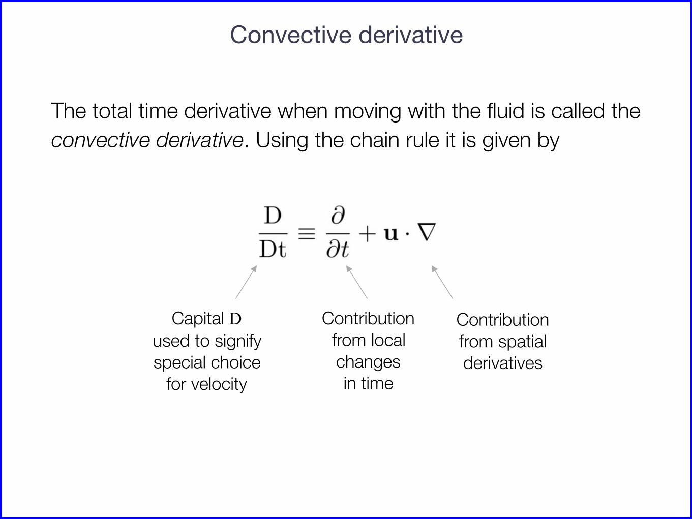
Convective derivative

The total time derivative when moving with the fluid is called the convective derivative. Using the chain rule it is given by

Capital D used to signifyspecial choice

for velocity

Contributionfrom localchangesin time

Contributionfrom spatialderivatives

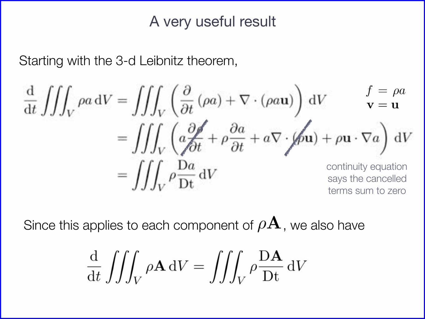
A very useful result

Starting with the 3-d Leibnitz theorem,

Since this applies to each component of , we also have

continuity equation says the cancelled terms sum to zero

Momentum equation (Newton’s 2nd law)

Newton's 2nd law: The rate of change of an object's momentum is equal to the sum of the forces acting on the object (F = ma).

The momentum per unit mass is the velocity, so

Consider two types of forces: • Body forces act within the volume, e.g. gravity. • Contact forces act on the surface that bounds the volume.

Momentum equation (Newton’s 2nd law)

The total body force acting on the volume

will therefore be

Introduce as the body force per unit volume, e.g. gravity contributes

Body forces Contact forces

Total is determined by integrating contact force per unit area over

the bounding surface.

If the only contact force is pressureacting normal to the surface, ,

the total contact force on V is

Momentum equation (Newton’s 2nd law)

Matching the two sides of Newton’s 2nd law therefore gives

If true for any volume of fluid, then everywhere

Note: Often need a more general treatment of contact forces. An important case is the Navier-Stokes equation with viscosity

Energy equation

Our model conserves mass and momentum. Does it conserve energy?

Body forces

Contact forces

Rates at which forces do work Change of kinetic energy

Work of compressing the volume is unaccounted for!

Energy equation (1st law of thermodynamics) Fix: include the fluid’s internal energy

Introduce as the specific internal energy density, i.e. per unit mass.

Internal energy of a volume of fluid =

The first law says internal energy changes through work and heating.

If true for any volume of fluid, then everywhereheating rate

per unit volume

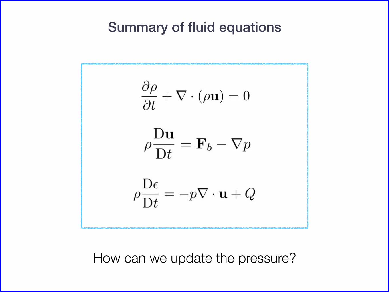
Summary of fluid equations

How can we update the pressure?

Closure (LTE equation of state)

For an ideal fluid in local thermal equilibrium, i.e. assuming collisions have made the particle distribution a drifting Maxwellian, find:

Numerically, can calculate as needed.Strategy 1:

or

Eliminate

Strategy 2:

Summary of fluid equations

Where closure was by assuming LTE.

Single-fluid resistive MHD

Macroscopic method

Fluid equations

closure by assuming ideal gas relations: LTE

E.M. equations

Fluid equations

E.M. equations

1. After applying body forces and Ohmicheating rate

2. Will set v = u.

3. Curl of Faraday’s law implies div(B) remains zero, so don’t need div(B) =0 as a separate condition.

Fluid equations

E.M. equations

4. Neglect displacement current and Coulomb force based on “quasi-neutrality”. Dimensional analysis indicates this applies when phase and fluid speeds are much less than speed of light. Sometimes called the MHD approximation.

At that point can drop Gauss’ law.

Fluid equations

E.M. equations

5. Eliminate j using Ampère’s law, and E using Ohm’s law, which can then be dropped.

E.M. equations

Fluid equations

MHD equations

Assumptions used

• Fluid • LTE • Ohm’s law• Isotropic pressure

• Quasi-neutrality (velocities much less than c)

Magnetic forces

magneticpressure

term

magnetictension

term

The perpendicular part of the “tension” term is

Standing coronal loop oscillations excited by flare (magnetic tension): see http://adsabs.harvard.edu/abs/1999Sci...285..862N

http://adsabs.harvard.edu/abs/1999ApJ...520..880A

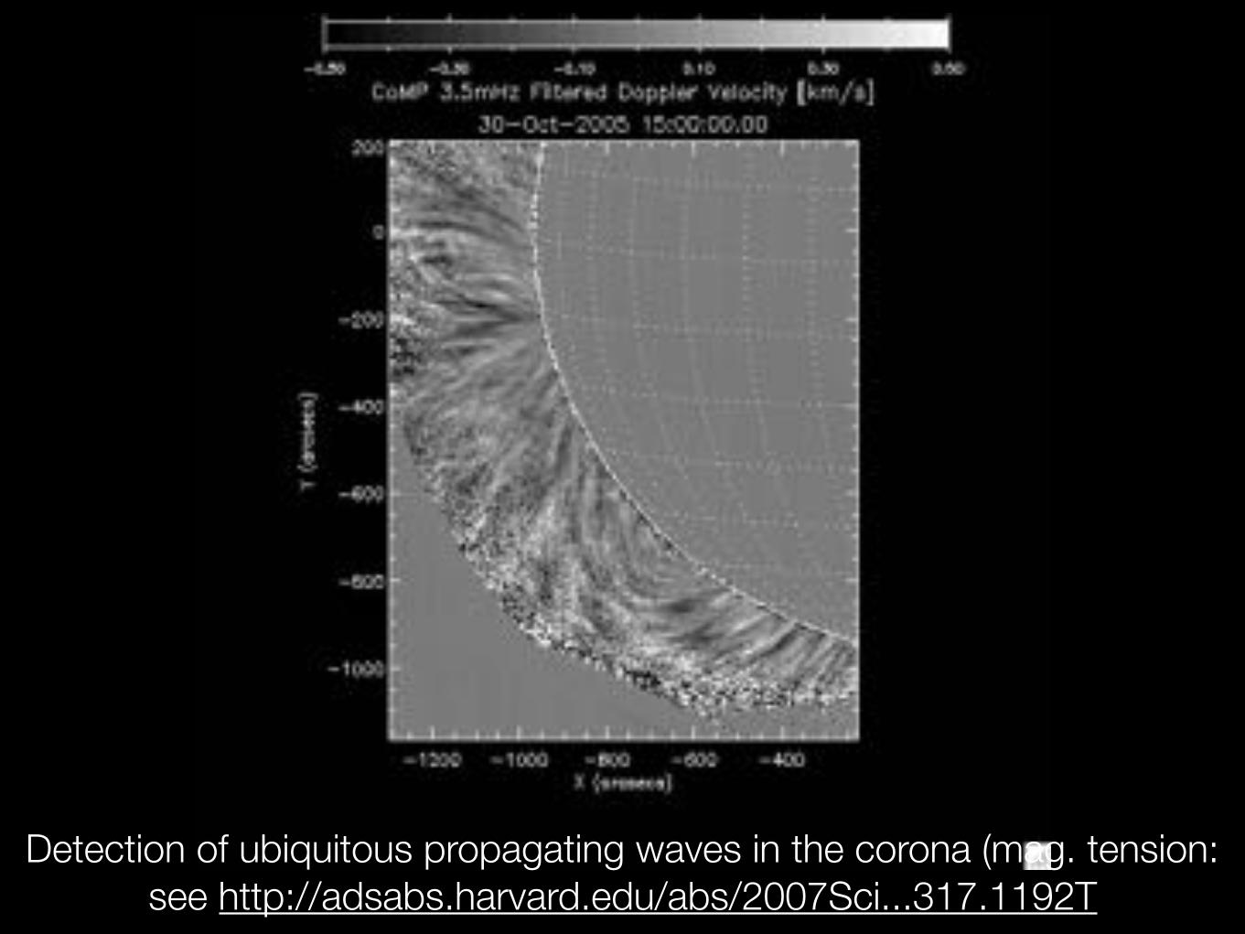
Detection of ubiquitous propagating waves in the corona (mag. tension: see http://adsabs.harvard.edu/abs/2007Sci...317.1192T

Magnetic forces

magneticpressure

term

magnetictension

term

Thermal pressure is proportional to internal energy per unit volume. Magnetic pressure is is proportional to magnetic energy per unit volume.

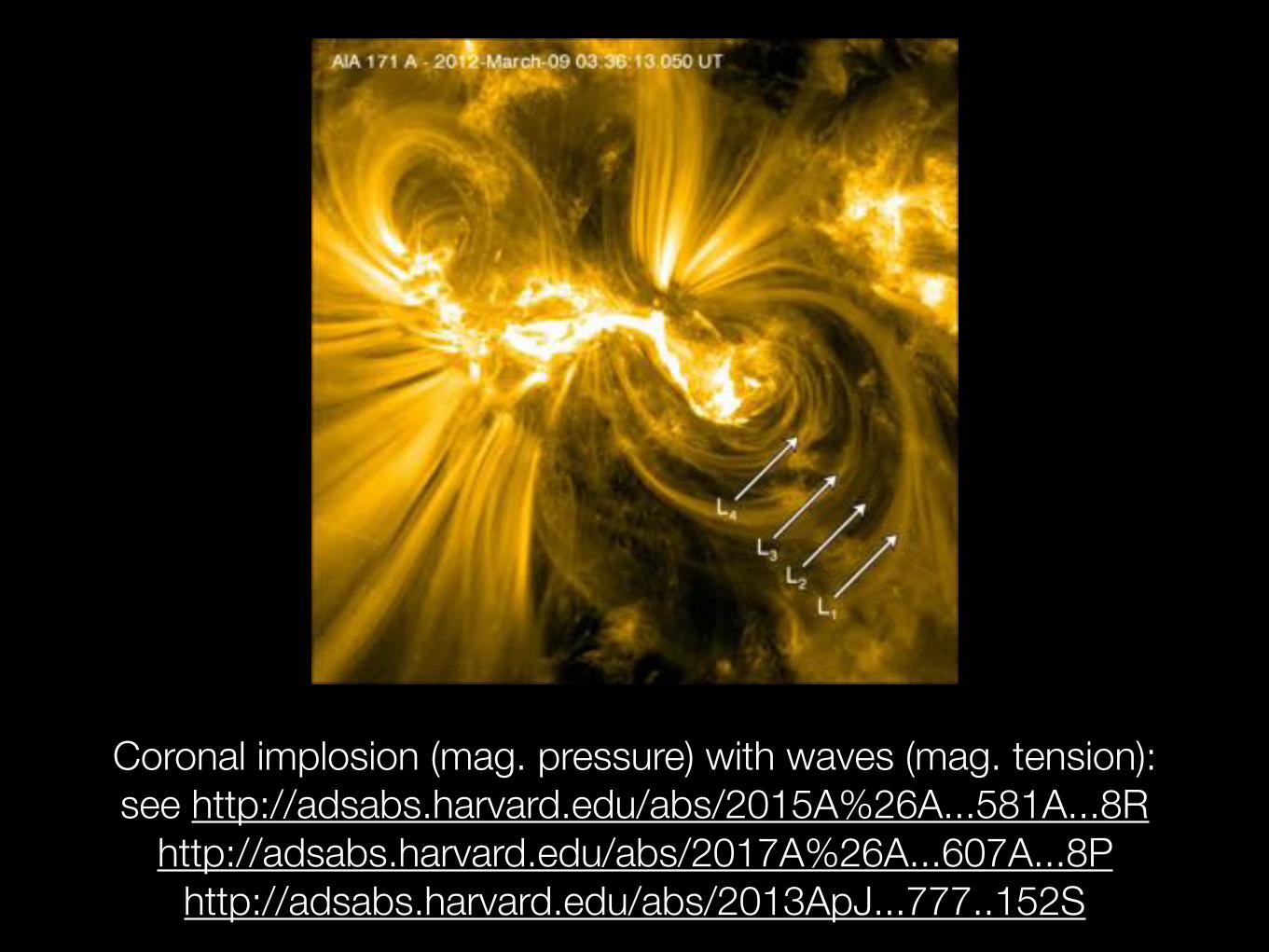
Coronal implosion (mag. pressure) with waves (mag. tension): see http://adsabs.harvard.edu/abs/2015A%26A...581A...8R

http://adsabs.harvard.edu/abs/2017A%26A...607A...8P http://adsabs.harvard.edu/abs/2013ApJ...777..152S

Thermal pressure forces

-6000 -4000 -2000 0 2000 4000Height (km)

10-1

100

101

102

103

104

105W

ave

speed (

km/s

)

vA

cs

Alfvén and sound speeds in the Sun

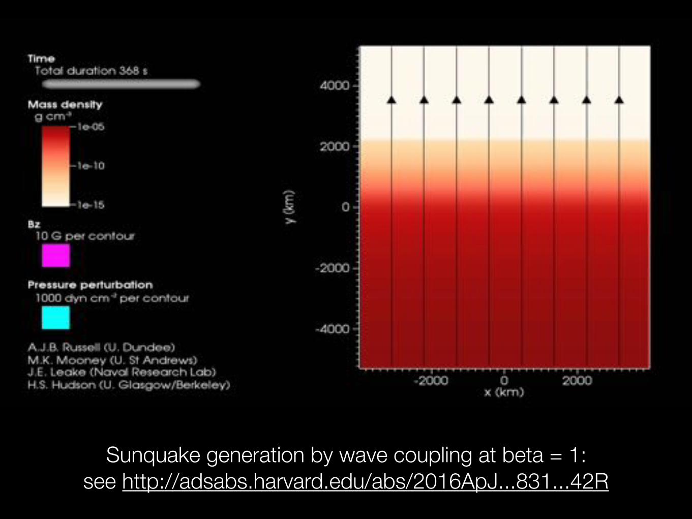
Sunquake generation by wave coupling at beta = 1: see http://adsabs.harvard.edu/abs/2016ApJ...831...42R

PROPERTIES OF FLARES-GENERATED SEISMIC 7

Figure 2. A white-light image of active region NOAA 10696 observed on October 28, 2003, andsuperimposed images of the Doppler signal at the impulsive phase, 11:06 UT (blue and yellow spotsshow up and down photospheric motions with variations in the MDI signal stronger than 1 km s−1),positions of three wave fronts at 11:37 UT, and also locations of the hard X-ray (50 – 100 keV) sources(yellow circles) at 11:06 UT and 2.2 MeV γ -ray sources (green circles).

was not detected for other seismic events. However, the strong photospheric motionsobserved in the Doppler signals at 11:06 UT show the best correspondence to thecentral positions of the wave fronts. This leads us to the conclusion that the origin ofthe seismic response is the hydrodynamic impact. This was verified by calculatingthe time–distance diagrams for various central positions and various angular sectors.When the central position of a time–distance diagram deviates from the seismicsource position, this deviation is immediately seen in the diagram as an off-setof the time–distance ridge. This approach provides effective source positions forcomplicated and distributed Doppler signals.

2.3.2. X1.2 Flare of January 15, 2005The flare of January 15, 2005, was of moderate X-ray class, X1.2, but producedthe strongest seismic wave observed so far by SOHO (Figure 1, bottom row). Itsamplitude exceeded 100 m s−1. This wave had an approximately elliptical shapewith the major axis in the SE – NW direction. This shape corresponds very wellto the linear shape of the seismic source extended in this case along the magneticneutral line. This is illustrated in Figure 3. The left panel shows the gray-scale mapthe Dopplergram difference at 0:40 UT, in which the long white feature near thecenter corresponds to strong down flows at the seismic source, and an image ofthe hard X-ray source (color spot). The right panel shows the corresponding MDImagnetogram and an image of the soft X-ray emission (in gray) and contour line

Kosovichev 2006

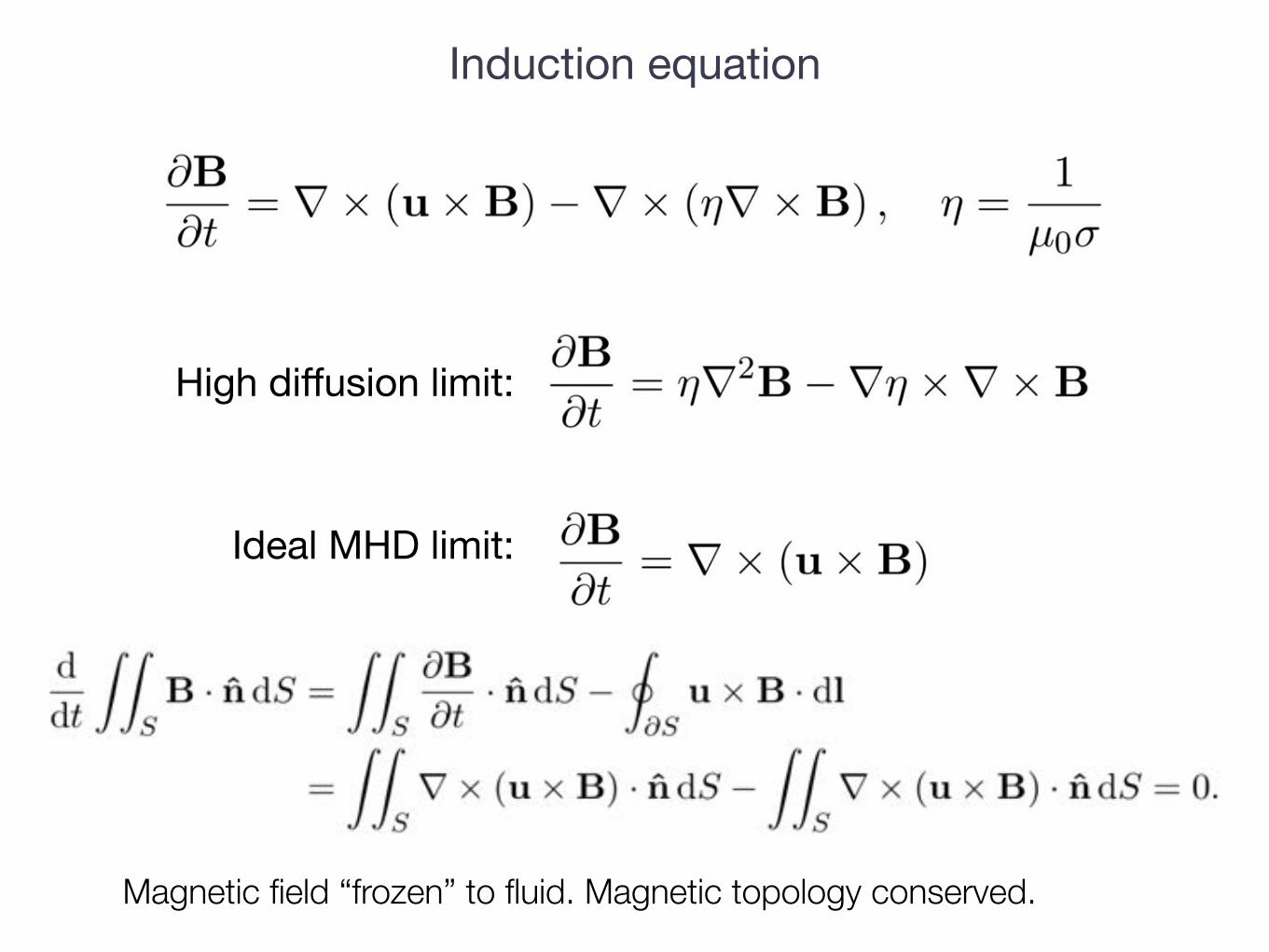
Induction equation

High diffusion limit:

Ideal MHD limit:

Magnetic field “frozen” to fluid. Magnetic topology conserved.

MHD simulation of fast triggered magnetic reconnection (high Rm): see http://adsabs.harvard.edu/abs/2012ApJ...760...81K

MHD simulation of a turbulently reconnecting magnetic braid see http://adsabs.harvard.edu/abs/2016PPCF...58e4008P

http://www.maths.dundee.ac.uk/mhd/pubs.shtml

MHD equations

Assumptions used

• Fluid • LTE • Ohm’s law• Isotropic pressure

• Quasi-neutrality (velocities much less than c)