Compurws Ckm. Vol. 15, No. I, pp. F&72, 1991 OOY7-8485/91 53.00 + 0.00 Printed in Great Britain. All rights reserved Copyright 0 1991 Pergamon Press plc

GENERAL LINEAR REGRESSION ANALYSIS- APPLICATION TO THE ELECTRIC DIPOLE-MOMENT

FUNCTION OF HCl

J. F. oGILVIE*

Department of Chemistry, National Tsing Hua University, Hsinchu 30043, Taiwan and Academia Sink, Institute of Atomic and Molecular Sciences, P-0. Box 23-166, Taipei 10764, Taiwan

(Received 27 Feebruary 1989; in revised form 7 March 1990; received for publication 12 June 1990)

Abstract-The program GWLREG has been designed for the convenient and efficient treatment of general iproblems in linear regression, including both multiple linear and univariate polynomial forms. There is brovision for transformation and weighting of input data, and output of indicators of goodness of fit. Two versions of the program GWLREG are presented, each based on a different computational algorithm and having slightly differing capabilities and performance. The program is applied to a new determination of the electric dipole-moment function of the diatomic molecule HCl from a critical assessment of the published experimental data.

1. INTRODUCTION

The mihimum attributes of a satisfactory computer program for linear regression applications are the followiag:

adequate accuracy; indicators of goodness of fit; simplicity of use and adaptation for particular problems; capability of weighting the input data; automatic transformation of input data; applicability of simple constraints, such as passage through the origin.

The author has been unable to discover a single program for microcomputers that has all these essen- tial attributes and is applicable to both univariate polynomial and multiple uninomial linear regression. For this reason I have undertaken to develop the program GWLREG. For reasons of convenience, this paogram has been prepared in BASIC, a language commonly available on microcomputers, in order bo generate in the most convenient analytic form a representation of these data. In this paper we discuss the algorithms and their new implementation in the two versions of the program GWLREG, and then apply it in order to determine the polynomial funvtion to represent the radial dependence of the electric dipole moment of a diatomic molecule.

2. MATHEMATICAL BASIS OF THE ALGORITHM

If we suppose that we have a set of n observations involving the independent variables x,, 1 ci 6 k, and

*All eoarespondence should be addressed to the author at the Academia Sinica address above; electronic mail to ogiluie@twniams.bitnet.

the dependent variable y, then as long as k c n, the coefficients /$ of nj are overdetermined. In these circumstances the statistical fitting of the data, sub- ject to some experimental error e assumed to be entirely associated with the dependent variable y and to be independent of the particular value of y, becomes the appropriate procedure according to the standard theory of regression analysis_ If, further- more, the values of y depend upon the parameters 8, in a linear manner, then the approach of linear regression may be used, much simpler and more direct than nonlinear parameter estimation. The values of the parameters bi are the best, i.e. most precise and unbiased, estimates of the unknown quantities p, if the criterion to determine them is the minimum value of the sum of the squares of the residuals

over the R items in the data set; if b, is present (x0 = 1) and has a value significantly different from zero, then the function does not pass the origin of the coordinate system having k dimensions.

The algorithms, to be discussed in the following paragraphs, were programmed in BASIC for the following reasons: this computing language is widely used on l&bit microcomputers of the type called personal computer; the program is easily written in this language: unlike FORTRAN, in compiled BASIC a program is prepared into an efficiently executing form in only one brief stage, without several passes for compilation and linking. Also, despite the fact that interpreted BASIC executes less rapidly than compiled BASIC, program preparation and testing is more conveniently conducted in the former way; moreover, no changes may be necessary

59

60 J. F. Oor~vt~

if one later resorts to compilation in order to improve speed of execution.

As a strategy for the construction of the new program GWLREG, it was decided to use as a basis the program MULNRG (Ogilvie & Abu-Eigheit, 1981) that was designed for only unweighted multiple linear regression. Thus, we first describe the math- ematical basis of the algorithms of GWLREG con- taining the enhancements and extensions beyond MULNRG for the present objectives. We state the basic problem in matrix form, for each data set:

((~1) = ((x)) ((4

in which ((x)) is a row matrix (or vector) of length k + 1 representing the values of the independent variables, ((b)) is a column matrix also of length k + 1 representing the values of the parameters to be determined according to the principle of least squares and ((y)) is thus a matrix of order 1 (equivalent to a scalar). The addend 1 in k + 1 results from the fact that, in the first instance, the function is not con- strained to pass the origin; in that case the numbering of the elements of ((x)) and (@)) starts at zero and x,, = 1. The data to be analyzed consist of II sets, the ith set containing the k values of the independent variables +, 1 <j < k, the value of the corresponding dependent variable yi, and the weight wi which may simply be the reciprocal of the variance (the square of the standard deviation) of the value of y; deter- mined as the result of replicated trials under the same conditions (i.e. the same vaIues of x5)_ In order to determine the ((b)) matrix, we must form two other matrices, the symmetric square matrix ((a)) of order k + 1 and the column matrix ((g)) of order k + 1 having elements as follows:

aa,0 = c wi,

a,, = z xjixli wi, 0 <j, I < k, j 6 I,

g0 = CYiwi3

gj = C xjiyi w,, 1 <j < k.

In each case it is to be understood, here and else- where unless otherwise specified, that the summation Z is over the values of i, 1 6 i d n, in the data set. The ((a)) matrix is then the product of the inverse, ((d)) of the ((n)) matrix with the (Cg)) matrix:

((4) = ((a))-’

and

((b)) = (V)) ((s>).

We need also to calculate the sum of the squared errors (SSE), which can be formed from the ((d)) and ((g)) matrices and the transpose ((g))’ of the ((g)) matrix:

SSE = ((g))‘((g)) - ((4)((g)),

although computationally it is better to calculate SSE directly from the definitions (expressed in both the

matrix form and the non-matrix form actually used in the program):

SSR - ((Y))‘((Y)) - 2(@))(x))‘((~))

+ 0)) ((x))‘((x)) ((3))

We define another column matrix ((s)) of order k + 1 of which each element sI is the standard error, the square root of the variance, of the corresponding elements of the parameter matrix ((a)):

s, = @!!SSE/~)“*,

in which f is the number of degrees of freedom of the regression process, equal to the number n of data sets minus the number of parameters k + 1. The other essential indicators of the goodness of fit are:

the standard deviation Q of the fit,

the absolute value Irt of the sample correlation coeiiicient r,

and .the F statistic or F-value (Ogilvie & Abu- Elgheit, 1981),

The square dispersion matrix ((v)), the product of the inverse of the ((a)) matrix with the error variance oz of regresion,

((0 )) = a’(V))*

contains as its elements vu- along the principal diag- onal the variances of the b parameters,

vjj = sj,

whereas the off-diagonal elements are the covariances that contain information about the correlation of the nominally independent parameters, the regressor matrix ((h)) that is formally the primary objective of the regression analysis. The elements c,, of the par- ameter correlation matrix, a more useful visual indl- cator of the independence of the 4 parameters, are formed simply by dividing the covariances by the square root of the product of the corresponding product of variances,

9, = ~,,l(~,,~,,Y,

General linear regression analysis 61

but in the prediction of new values of the dependent variable yprod from the specified values of the indepen- dent vagiables ((x)) and the determined parameter matrix,

&cd = ((x)) (@))

the variance, or square of the standard error, of the predicted value is most directly calcuiated from the variances and the covariances

In the case that the function y(x) is to be con- strained to pass the origin, i.e. when all xki= 0, k >O, then yi= 0, some equations above must be modified as follows, essentially to remove the zeroth row and the zeroth column from the ((a)) matrix and the zeroth element correspondingly from the ((g)) column matrix:

and

gj = c xJiYl “‘I 7 lGj<k.

Then the product of the ((d)) and ((g)) matrices is the @b)) matrix containing k elements starting with b, r leading to the variance of predicted values y- of the independent variable y according to the equation

The above description has been based upon the supposition that the independent variables x1, each unrelated to the other, are related to the dependent variable y ia a simply linear manner. For analysis according to the model of a polynomial in one independent variable, there is a trivial conversion,

xj=x{, j>l,

that has no other effect on the computational method, However, in practice, the magnitudes of the paramet.er correlation coefficients are then found generally to approach unity; this deficiency of a power sries is well known, but the practical utility of this form of model nevertheless makes it widely used. Other transformations of the independent variables can jusm as easily be effected, with no great effect on the nature of the computations. If the dependent variable y is however transformed from Y, then there must be an appropriate global weighting factor W = (d Y/dy)’ applied (de Levie, 1986) further to any specific weight w, arising from the standard deviation of any particular value Yi.

The aoding of the above equations into a computer program in two versions, each with adequate accu- racy, suffices to achieve the objectives of the present work.

3. IMPLEMENTATIONS OF THE ALGORITHM AND TFSTING

In the Cd version, the program GWLREG in BASIC consists of ten sections: initiation; variable transformation; control; data input; data correction; computation of results; output of basic results; out- put of table of residuals; output of parameter corre- lation coefficients; and termination. The initiation section declares the variables to be either double precision in floating point or integers and prints a heading. The variable transformation section consists of three function statements that convert all the independent and dependent variables and the weights into the appropriate form according to the particular application. The function to form the weight can incorporate any global weighting factor that may be required. In the control section, the user is prompted to ascertain whether either multiple linear or poly- nomial regression is required, the number of indepen- dent variables if the former or the maximum degree of the polynomial and whether results for lesser degrees are required if the latter, and finally whether the constraint of passage through the origin is to be applied. In the data input section, the number n of data sets is demanded, followed by a prompt for each value of xJi, y, and the particular weighting factor wj (further to the global weighting factor automatically applied according to the appropriate function state- ment). These values are displayed compactly on the monitor screen so that visual inspection of their correctness is easily achieved. If no input data are to be corrected, according to the prompt at the end of the data input, then the computation begins, and the output of the basic results automatically proceeds. Next the user is prompted for output of first the table of residuals then the table of parameter correlation coefficients cj,, The user is then prompted to delete any data cases, and to add further data cases; if there are any such deletions or additions then the computation of results is repeated. If there are no such alterations to the input data, either the program terminates for the case of the multiple linear regression and the polynomial regression at the maxi- mum degree, or the program continues with the next higher order of polynomial regression according to the control parameters input at the beginning of the run.

The testing of GWLREG has been conducted in several ways. First of all, because the entire accuracy of the analysis depends vitally on the inversion of the ((a)) matrix, this subroutine was separately tested. Three different methods of matrix inversion were tried; one employed the Gauss-Jordan elimination method and a second, using an alternative elimin- ation approach, was the MINV subroutine translated from FORTRAN. As Crout’s method of decompo- sition with partial pivoting (Golub & van Loan, 1983), followed by iterative improvement, gave superior results, although requiring a somewhat greater storage space for arrays (Press et al., 1985),

62 J. F. 0omw.e

this procedure was incorporated into the Cd version of GWLREG. The test was the Hilbert matrix in which the value of each element is the reciprocal of the sum of the subscripts, i.e.

this matrix is notoriously ill-conditioned and is there- fore an exemplary, critical and pertinent test of the inversion process.

At this point it becomes necessary to specify the varieties of BASIC used for the calculations. Three varieties have been tested, BASICA, Turbo-BASIC and Professional BASIC. The latter is most con- venient when one types in the program because it prompts as soon as most common typing errors are made, but because it, like BASICA, is interpreted BASIC it executes relatively slowly. Turbo-BASIC is compiled and consequently executes rapidly. Because these regression calculations require only a few seconds, the execution time, in any case commonly less than the time to print the results, residuals and correlation coefficients, is much less a matter of concern than the numerical accuracy. There is in principle a significant difference between BASICA which carries 17 decimal digits and the other two which carry only 16 decimal digits of precision_ For instance, in the inversion of the Hilbert matrix of order 6 by the Gauss-Jordan method, BASICA yields 10.1 correct digits on average, whereas the other processors yield 9.3 correct digits on average; for the Hilbert matrix of order 8, BASICA yields 7.2 correct digits, compared with 6.3 digits for the other specified processors. By Crout’s method, the average number of correct digits is 11.3, 10.2 or 11 .O for the matrix of order 6 and 9.0, 7.7 or 8.0 for order 8 by BASICA, Professional BASIC or Turbo-BASIC, respectively. However, it should be noted that the greater precision in BASICA is accompanied by the small range of exponent (- lo*‘*) and the evaluation of numerical functions in only single precision even if the argument is double precision, whereas both Professional BASIC and Turbo-BASIC provide a much greater range of exponent (- 10i308) and the evaluation of numerical functions of double-precision arguments (and in Turbo-BASIC even single-precision argu- ments) in double precision. For the range of values in the matrices under test, the difference in precision between these processors is significant, and obviously the requirement of matrjx inversion may prove the factor ultimately limiting the accuracy in permitting any program incorporating such a subroutine to produce significant results for high orders of the matrix to be inverted. Furthermore, although the gain in precision in the matrix inversion from Crout’s decomposition over the Gauss-Jordan method is substantial, in the subsequent solution of the normal equations the iterative approach provides even fur- ther improvement. An alternative algorithm involv- ing the direct factorization of the matrix of the coefficients of the normal equation according to

Doolittle’s approach produced essentially identical results to those from Crout!s decomposition.

The second version (svd) of the program GWLREG resembles the first (Cd) except that, instead of an algorithm intended to solve the normal equations, the method of singular-value decompo- sition used (Golub & van Loan, 1983). Thus, the substitution subroutine and the main ,section of the Cd version in which the matrix of the coefficients of the normal equations is effectively inverted are replaced by several loops which serve to solve directly the design matrix (the set of linear equations, one for each data set, in which the regression coefficients appear as the unknown parameters) by decompo- sition of its singular values.

The second kind of test of the accuracy and efficiency of both versions of GWLREG involved the test problems used by Wampler (1969) in this evalu- ation of the then available computers and programs for linear least squares. These are the two poly- nomials of order 5, identified as Yl and Y2:

Yl: Y&j j-0

and

Y2: y = i (x/io)j, j-0

with values of x, being the integers between 0 and 20; for the test of the cases constrained to pass the origin, the constant term (1) was omitted from both Yl and Y2. For these four cases, i.e. Y l(l), Y2(1), Yl(0) and Y2(0) with 1 and 0 values of the

y-intercept, respectively, the results are given in Table 1 for the cases of the three processors and the two algorithms. The indicators of the goodness of fit that are shown in the table are the F-value, for which a greater value is desirable, the standard .deliation of the fit, for which a smaller value is desirable, and the average number of correct digits in the derived parameters 4, 0 <j < 5 or 1 <j < 5, for the two values, 0 or 1 respectively, of the y-intercept. The results appear to demonstrate that for the implemen- tation of the Crout decomposition BASICA is the best of the three processors, based on the average number of correct digits being greatest in most test cases, although it should be noted that for Y l(1) and Y2(0) the standard errors of the regression parameters were in some cases significantly smaller for Turbo-BASIC than for BASICA. In contrast, the results (not shown) for BASICA for the svd algorithm are relatively poor. Due to the latter qualifications, to the generally useful more extensive range of exponents in Turbo-BASIC and to the greater speed of execution of Turbo-BASIC, this processor may be preferred for use with either version of GWLREG.

Comparison of the results for Y l(1) and Y2( 1) in Table 1 should also be made with the results in Wampler’s (1969) report. In that case the average

General linear regression analysis

Table 1. Comparison of results for the test regression problems by means of the algorithms using Grout decomposition (Cd) or singular-value &composition (svd) with the interpreters BASICA (BA) and Professional BASIC (PB) and the compiler Turbo-BASIC (TB); the criteria arc the F-value Q,

the standard deviation of the fit (a) and the average number of correct digits (No.)

Cd svd

BA PB TB PE TB

YW) F 1.1 x ion 6.0 x IO” 2.0 x 1p 1.7 x I@’ 7.3 x 103’

:o. 1.8 x IO-’ 7.9 x 10-S 4.3 x 10-q 4.7 x lo-‘0 2.3 x IO-‘0

8.0 7.5 9.3 11.3 11.3

YW) F 3.2 x Ion 4.3 x w 7.8 x 1026 2.5 x lo= 8.0 x 1oU

FJo. 6.4 x lo-” 9.4 x 10-a 1.3 x lo-” 7.2 x lo-” 1.2 x 10-I’

10.0 8.8 9.6 9.7 9.7

63

WO) F 1.8 Y ldn 1.9 x 10’6 2.0 x 10% 2.1 x lo-” 4.1 x lo-” k*. 4.5 x 8.4 10-a 2.7 x 9.6 IO-” 1.3 x 7.4 10-l 4.3 10.2 x 10-10

y--w F 6.9 x Id’ 3.7 x IO” 1.6 x lp6 2.6 x It?’ 8.0 x 10” zkl. 1.4 x 10.4 10-I’ 1.9 x 9.4 lo-‘2 2.9 x 9.4 lo-” 7.2 x 9.5 lo-” 1.3 x 9.7 lo-”

numbeti of correct digits for double-precision runs with 16 digits were 6.9 and 7.9 for Yl and 6.2 and 10.0 for Y2, although for double-precision runs with 18 digits the average numbers of correct digits were at least 9.3 for Yl and Il.8 for Y2 when elimination methods were used and generally more for other methods. Thus, because. the present results producing up to lg.3 correct digits for Yl(1) and 10.0 for Y2(1), respectively, are at least of the same order of magni- tude as for the programs that Wampler (1969) tested, one may conclude that GWLREG is thus likely to be acceptable as a general routine for applications in lineai regression, within the limitations mentioned above.

4, AF’PLXATION TO THE ELECl-RIC DtPOLEMOMENT FUNCTION OF HCI

In this application of the program GWLREG, we use not only the features discussed above but also thesprovision for weighting the input data. The latter pnavisian is crucial in this case because both the valqes of the dependent variables, the matrix elements <vJ/ M(x) Io’J’) of the dipole-moment function1 between vibration-rotational states specified by the quantum numbers D for vibration and J for rotation, and their nominal standard deviations vary over comparatively large ranges. The independent variable8 in this problem are the matrix elements (vJI_dla’J’> of the displacement x to various powers

j, which are roughly proportional to 10-i. Therefore, the test problem YZ(0) with k = 8 and using the Grout decomposition method is the most suitable to simulate the actual problem; running this problem with 0 $x < 32 produced an F-value 5.7 x 10” and a standard deviation of the fit 2.6 x lo-* with at least 5 accurate digits for each regressor. As the conditions of this test are much more severe than in the actual problem, this performance is considered acceptable.

The electric dipole-moment function M(x) of HCl may be expressed (Ogilvie & Tipping, 1983) in the form of a polynomial in the reduced internuclear displacement variable x in terms of the instantaneous R and equilibrium 4 internuclear separations. The power series which is truncated as required to fit the finite data, in this case at the seventh order,

has been determined anew from the available experimental data, namely the expectation values <vJ 1 M(x)1 vJ) of the dipole moment in particular vibration-rotational states, measured by means of experiments on the electric resonance spectra at radio frequencies on molecular beams using the Stark effect, and the matrix elements <$4(x)(0’> related to the intensities of vibration-rotational bands in the IR and VIS spectral regions. The data of Kaiser (1970) for the expectation values of the dipole moments of H”C1 and D”Cl were corrected for the deviation from the standard for such measurements [ground state of OCS (de Leeuw & Dymanus, 1970); corrected value for 1986 values (Cohen & Taylor, 1987) of the physical constants is (2.385558 k 0.00010) x 10e3’ C m] and for the change in the fundamental physical constants since 1970; these corrections are not much greater than the experimental uncertainties (taken as 3.5 SE) quoted by Kaiser. The analogous datum of de Leeuw & Dymanus (1973) for H3’Cl was also corrected, but only for the change in the phys- ical constants. The data for the intensities of the vibration-rotational bands were used without correc- tions, and in most cases with the acceptance of their nominal standard deviations. Measurements of these intensities have been carried out for several decades, during which period both spectral resolving power and the precision of measurement have increased greatly. For the fundamental and first-overtone bands, many data are available, listed by Pugh & Rao

64 1. F. OCXL~IE

(1976) and by Smith et al. (1985). Among these data for either band, the values range widely, far beyond the nominal uncertainties of the measurements. In particular, the data of Benedict et al. (1957), part of an extensive collection, have been found to be too small by comparison with more recent measurements; for this reason, all the data reported by these authors were arbitrarily assigned a further weighting that caused these values to have practically no e&t on the final results. Other data listed in the specified compilations have been omitted because the values are obviously inconsistent with more recent and presumably more accurate values. Specifically, the value by Smith (1973) for (O(M(x))2), a weighted mean of data that he then considered useful, has been omitted here because it is significantly smaller than real experimental values obtained both before and since that time. Similarly, the value of Benedict et al. for (1957) for <OIM(x))3) is confirmed to be too small (Stanton & Silver, 1988). For Kaiser’s (1970) data of DCl, it proved impossible to fit simul- taneously these data and all the data of HCl within reasonable bounds of uncertainties in relation to the nominal experimental errors; for this reason, these data of DC1 were also arbitrarily assigned the same standard further weighting that removed the sensi-

tivity of the results to these values. Kaiser attributed the inconsistency of these values of the expectation values of HCl and DC1 to a possible breakdown of the Bornappenheimer approximation, but an alternative explanation based on the inadequacy of the treatment of the rotational dependence of the expectation values has also been proposed (Ogilvie, 1988).

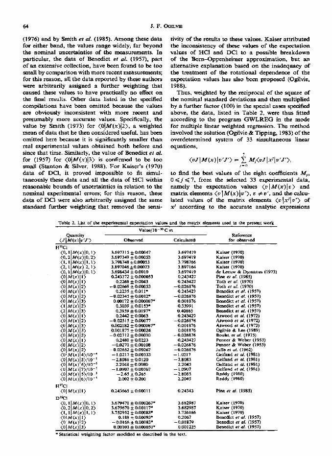
Thus, weighted by the reciprocal of the square of the nominal standard deviations and then multiplied by a further factor (100) in the special cases specified above, the data, listed in Table 2, were thus fitted according to the program GWLREG in the mode for multiple linear weighted regression. The method involved the solution (Ogilvie & Tipping, 1983) of the overdetermined system of 33 simultaneous linear equations,

to find the best values of the eight coefficients Mj, 0 <j $7, from the selected 33 experimental data, namely the expectation values <u ) M(x)(v > and matrix elements <v 1 M(x)lu’), v # v’, and the calcu- lated values of the matrix elements (v Ix/l o’> of xj according to the accurate analytic expressions

Table 2. List of the experimental expectation values and the matrix elements used in the present work

Value/lo-“Cm

&Y$&,> Reference

Observed Calculated for observtd

H”Cl

(0 M(x) 4>/10-4 <o M(x) 5>/10-’ (0 M(x) 6}/10-’ (0 M(x) 7>/10-’ <o M(x) s>/lom (0 M(x) 6)/10-’

H”CI <OlwG(l>

D”CI (0, 1 M(x) 0, (0.2 M(x) 032)

I I

1>

<I, 1 M(x) 1, I> <o Jwx1 I>

I I <o M(x) 2>

3.6973 I5 f 0.00047 3.697349 f 0.00053 3.798748 *0.00053 3.897046 4o.ooo73 3.698434 f 0.0010 0.243372 f O.OOtX53

il.2268 f 0.0043 -0.02669 f omOs3

0.2235 f O.Oll* -0.02345 f 0.0012”

0.00172 f 0.000087* 0.3039 f 0.0 153’ 0.3959 f 0.0197* 0.2442 f 0.0063

-0.02515 f 0.00077 0.002182 f 0.000087* 0.001875 f O.ooO24

-0.02712 f O.OtM30 0.2480 f 0.0223

-0.0270 f 0.00108 -0.02652 f 0.00267

-1.0217 f 0.00333 -2.8086 f 0.0120

2.2048 f OXi - 1.0907 f 0.00367

-2.65 f 0.265 2.002 f 0.200

3.697419 3.697419 3.798766 3.897164 3.6974 I9 0.243427 0.243427

-0.026876 0.243427

-0.026876 0.001876 0.33991 0.4086S 0.243427

-0.026876 0.001876 0.001876

-0.026876 0.243427

-0.026876 -0.026876 -1.0217 - 2.8083

2.204s -1.G907 - 2.8083

2.2045

Kaiser (1970) Kaiser (1970) Kaiser (1970) Kaiser (1970) de Lceuw & Dymanus (1973) Pine er rrl. (1985) Totb et nl. (1970) Totb et uL (1970) Benedict et al. (1957) Benedict et 01. (1957) Benedict et al. (1957) Benedict et al. (1957) Benedict et al. (1957) Atwood el al. (1972) Atwood et oi. (1972) Atwood er al. (1972) Ogilvie & Lee (1989) Boulet et ol. (1975) Penner & Wcber (1953) Penner & Webet (1953) Iaffe et al. (1962) Gelfand e& al. (1981) Gelfand er al. (1981) Gelfand ef al. (1981) Gelfand et al. (1981) Reddy ( 1980) Reddy (1980)

0.243665 f 0.0001 I 0.24343

3.679470 f 0.000267* 3.682987 3.679670 f 0.00117* 3.682987 3.752952 f 0.00083* 3.756166

0. I88 + 0.00093* 0.2067 -0.0166 f 0.00083* -0.01879

Pine et al. (1985)

Kaiser (1970) Kaiser (1970) Kaiser (1970) Benedict t-r al. (1957) Benedict er crl. (1957)

<olMw)l3> 0.00103 f 0.wOo50’ 0.001225

* Statistical weighting factor modified as described in the text.

Ekncdict et 4. (1957)

General linear regression analysis 65

(Bouanich et al., 1986) including terms containing (consistently) the potential-energy coefficients a, (Coxon & Ogilvie, 1982) in the Dunham (1932) function,

up to ,. “t

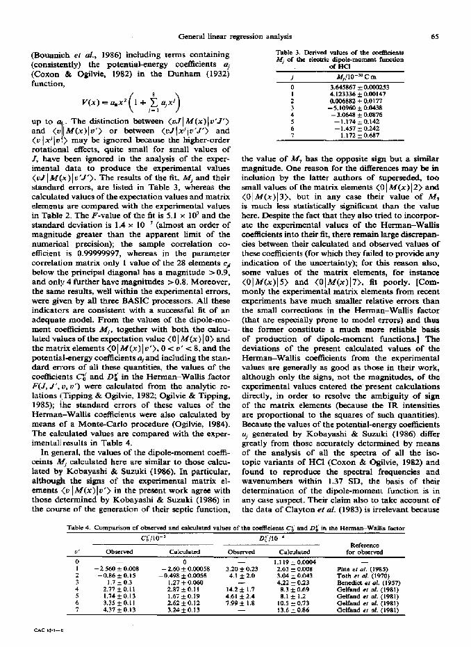
The distinction between <uJ 1 M(x) 1 u’J’> and (v lM(x)(v’> or between <uJ lx’1 v’J’> and {u Ix-‘lo!> may be ignored because the higher-order rotationial effects, quite small for small values of J, have been ignored in the analysis of the exper- imental data to produce the experimental values (uJ~MQx)~o’J’). The results of the fit, Mj and their standard1 errors, are listed in Table 3, whereas the calculated values of the expectation values and matrix elements are compared with the experimental values in Table 2. The P-value of the fit is 5.1 x lo7 and the standard deviation is 1.4 x lo-’ (almost an order of magnitude greater than the apparent limit of the numetiaal precision); the sample correlation co- efficient is 0.99999997, whereas in the parameter correlat/on matrix only I value of the 28 elements cir below the principal diagonal has a magnitude BO.9, and only, 4 further have magnitudes >0.8. Moreover, the same results, well within the experimental errors, were given by all three BASIC processors. All these indicatars are consistent with a successful fit of an adequate model. From the values of the dipole-mo- ment coefficients Mj, together with both the calcu- lated vallues of the expectation value <O 1 M(x) IO> and the matrix elements (0 1 M(x) I u’), 0 < tr’ < 8, and the potential-energy coefficients nj and including the stan- dard errors of all these quantities, the values of the co&icients Ct;’ and Dt;’ in the Herman-Wallis factor F(J, J’,Iu, u’) were calculated from the analytic rc- lations (Tipping & Ogilvie, 1982; Ogilvie & Tipping, 1985); the standard errors of these values of the Herman-Wallis coefficients were also calculated by means of a Monte-Carlo procedure (Ogilvie, 1984). The calculated values are compared with the exper- imentall results in Table 4.

In general, the values of the dipole-moment coeffl- ccints M, calculated here are similar to those calcu- lated by Kobayashi & Suzuki (1986). In particular, althouefh the signs of the experimental matrix el- ements (o I M(x) I u’> in the present work agree with those determined by Kobayashi & Suzuki (1986) in the course of the generation of their septic function,

Table 3. Derived values of the .meStcients M, of the cl&riic dipole-momant function

of HCl

i M,/lO-aCm 0 3.645867 * 0.000253 1 4.123336 & 0.00147 2 0.006882 + 0.0 177 3 -5.10960 * 0.0438 4 -3.0648 k 0.0876 5 -1.174 & 0.142 6 - 1.457 + 0.242 7 1.172 k 0.687

the value of M, has the opposite sign but a similar magnitude. One reason for the differences may be in inclusion by the latter authors of superseded, too small values of the matrix elements (0 ( M(x) (2> and <O)M(x)l3>, b t . u m any case their value of M, is much Iess statistically significant than the value here. Despite the fact that they also tried to incorpor- ate the experimental values of the Herman-Wallis coefficients into their fit, there remain large discrepan- cies between their calculated and observed values of these coefficients (for which they failed to provide any indication of the uncertainty); for this reason also, some values of the matrix elements, for instance (01 M&)15> and <OIM(x)17>, fit poorly. [Com- monly the experimental matrix elements from recent experiments have much smaller relative errors than the small corrections in the Herman-Wallis factor (that are especially prone to model errors) and thus the former constitute a much more reliable basis of production of dipole-moment functions.] The deviations of the present calculated values of the Herman-Wallis coefficients from the experimental values are generally as good as those in their work, although only the signs, not the magnitudes, of the experimental values entered the present calculations directly, in order to resolve the ambiguity of sign of the matrix elements (because the IR intensities are proportional to the squares of such quantities). Because the values of the potential-energy coefficients a, generated by Kobayashi & Suzuki (1986) differ greatly from those accurately de&mined by means of the analysis of all the spectra of all the iso- topic variants of HCl (Coxon & Ogilvie, 1982) and found to reproduce the spectral frequencies and wavenumbers within 1.37 SD, the basis of their determination of the dipole-moment function is in any case suspect. Their claim also to take account of the data of Clayton et al. (1983) is irrelevant because

Table 4. Comparison of observed and calculated values of the coefiicients Cg and Di in the Henna~WaHis factor

C$/lW LI:/10-’ Refereme

Observed Calculated Observed Calculated for observed 0 I.1 19 f 0.0004 -

-2.560 + 0.008 - 2.60 f 0.Ocm8 3.20fo.23 2.63 i 0.008 Pine er al. (1985)

-0.86*0.15 1.7*0.3 -0.498 1.27 f f 0.0056 O.OM) 4.1 - f 2.0 4.22 3.04 * + 0.043 0.23 Toth Benedict er al. et (1970) 41. (1957) 2.77 +O.ll 2.87+0.11 14.2 f I.7 8.3 * 0.69 Gelfand tv a/. (1981) 1.74+0.13 1.67kO.19 4.61 f 2.4 8.1 * 1.2 Gclfand LI nl. (1981) 3.35 f 0. I I 2.62fO.lZ 7.99 it 1.8 10.5 * 0.73 Gclfand ef a/. (1981) 4.37 f0.13 3.24kO.13 - 13.6 f 0.86 Gelfand et al. (1981)

66 J. F. OGILVE

the latter spectral data were also included in the analysis made by Coxon & Ogilvie (1982). It should be noted that the analysis of Clayton et al. (1983) is also suspect; because, for instance, the range of values of a, determined by Clayton et al. (1983) for IPCl and H3’C1 separately is 10 times the stated standard error, it is difficult to have confidence in the math- ematical significance of at least these error estimates, In a recent determination of the dipole-moment function of HCl, because Bouanich (1987) used terms up to only a, in the potential-energy function and in other quantities, his results are not as accurate as those presented here; moreover, his use of the super- seded values of <OIM(x)12> and <OlM(x)j3> means that, even within the Sited accuracy of the terms he retains, the results are obsolescent.

5. CONCLUSIONS

We have presented the mathematical basis for two versions of a new program for the general analysis of linear regression incorporating weights for the input data that may be based on both the standard devi- ations of these data and a global weighting factor that is required if the dependent variable has been transformed in a nontrivial manner in order to permit the linear regression. The implementation of this basis in both versions, Cd and svd, of the program GWLREG, listed in the appendices, has been tested both in its critical subroutine for matrix inversion and by means of standard functions (Wampler, 1969). For data sets with strongly correlated regressor vari- ables, the svd version is preferable. The program GWLREG has then been applied to the new determination of the electric dipole-moment function of the diatomic molecule HCl from the experimental data for the expectation values from the Stark effect and the matrix elements from IR intensities. The results will be used in a separate determination of the vibration-rotational Einstein coefficeints of HCI (to be published).

It should be noted that the new program GWLREG, based on previously developed algor- ithms and programs (Ogilvie & Abu-Elgheit, 1981), has many advantages because of both its flexibility (within the confines of linear regression models) and the range of indicators of goodness of fit. Even though one version may, on occasion, prove limited by the numerical presision involved in the procedure of matrix inversion, such cases will require extreme precision. Used in this version, the Crout method has been demonstrated to be very efficient in this appli- cation (F’ress el al., 1985). Although producing even greater precision, the other algorithm based on singu- lar-value decomposition requires about 60% greater storage area for arrays, has 30% more statements, and thus executes correspondingly less rapidly than the version based on the Crout decomposition. More- over, the application of the constraint of passage of the fitted function through the origin is more

difficult to accomplish in the svd version than in the Cd version, although in fact better results (i.e. much smaller residuals and correspondingly a smaller standard deviation of the fit) are obtained in the test programs Y 1 and Y2 if this constraint is not enforced. The comparative tests of the two versions to the solution of the normal equations or of the equivalent design matrix indicate that under these conditions the svd algorithm does not produce results greatly superior to the other; certainly in the actual application to the dipole-moment data the exper- imental error of the latter is much more important to the overall accuracy than the numerical limitations of either algorithm. Also, the implementation of the svd algorithm operates poorly with the BASICA interpreter, presumably because of the limitations of the exponent range thereof. For these reasons we present here both versions, Cd and svd, of the program GWLREG.

For comparison, another general routine for unconstrained parameter estimation (in FORTRAN and therefore much less easy to use on personal computers) in use in this laboratory can provide at least 14 significant digits of accuracy in the same regression problems Yl and Y2; this program utilizes the algorithm developed by Levenberg et al. (Osborne, 1972) and avoids the explicit inversion of a matrix by applying Gauss-Newton procedure starting from supplied initial estimates and (hope- fully) converging to the correct results. However, in this indirect approach, unlike the direct approach in GWLREG, the final results are dependent in principle on the choice of the initial estimates; such a disadvantage may be tolerable when for nonlinear regression models no direct approach is possible, but one would in general prefer to avoid any poss- ible arbitrariness of ‘the solutions to a physical prob- lem. The limitations due to numerical precision in GWLREG can essentially be ignored if and when a further variety of BASIC for personal microcom- puters becomes available that carries at least 20- and preferably 30---significant digits; the time is now ripe for such a development. Further extensions to GWLREG that one might contemplate are the provision of an automatic plotting routine (Ogilvie, 1986), which would however make the program less portable between different BASIC processors, and a subroutine for prediction (interpolation) of further values of the dependent variable for a given set of values of the independent variables, with full measure of the standard deviation of such predictions through the use of the parameter correlation matrix. The latter extension is trivial to program, but would require a specific inverse transformation of the depen- dent variable relative to that used in the regression analysis. Other transformations of input variable can be easily accommodated by means of the insertion of the necessary statements in the input section. The flexibility of BASIC as the language of this program GWLREG makes such modifications easy

General linear regression analysis 67

to carry out, with rapid subsequent recompilation if necessary.

Acknowledgemenls-I thank Dr L. Famell for helpful advice and the National Science Council of the Republic of China fad the support of a visiting research professorship.

REFERENCES

Atwood ti. R., Vu H. & Vodar B. (1972) 3. Phys. (Paris) 33, 499.

Benedict !W. S.. Herman R., Moore G. E. & Silverman S. (1957) ,T. Chem. Phys. 26, 1671.

Bouanich J. P. (1987) J. Qwmt. Spectrosc. Radiuz. Transfer 38, 89.

Bouanich J. P., Ogilvie J. F. & Tipping R. H. (1984) Corn&. Phys. Commun. 39, 439.

Boulet C,, Piollet-Marie1 E. & Levy A. (1975) Spectrochim. Acta 3#A, 463.

Clayton 4:. M., Merdes D. W., Pliva J., McCubbin T. K. & TippinF R. H. (1983) J. Mol. Spectrosc. 98, 168.

Cohen El R. & Taylor B. N. (1987) Rev. Mod. Phys. 59, 1121.

Coxon J., A. & Ogilvie J. F. (1982) J. Chew Sot. Faraaby Trans. ‘II 78, 1345.

Dunham J. L. (1932) Phys. Rev. 41, 721. Gelfand ;J., Zughul M., Rabitz H. & Han C. J. (1981)

.7. Q+t. Spectrosc. Radial. Transfer 24, 303. Golub Cid H. &van Loan C. F. (1983) Matrix Computations.

Johns Hopkins University Press, Baltimore, Md. Jaffe, J. Htr., Kimel S. % Hirshfeld M. A. (1962) Can. J. Phys.

40, 113. Kaiser E W. (1970) J. Chem. Phys. 53, 1686. Kobayas k L M. % Suzuki I. (1986) J. Mol. Spectrosc. 116,

422.

Stanton A. C. Br Silver J. A. (1988) Appf. Opt. 27, 5009. Tipping R. H. & Ogilvie J. F. (1982) J. Mol. Spectrosc. %,

442.

de Leeuut F. H. & Dymanus A. (1970) Chem. Phys. Lett. 7, Toth R. A., Hunt R. H. & Plyler E. K. (1970) J. Mol.

Specirosc. 35, 110. 288. Wampler R. H. (1969) J. Res. Nat. Bar. Stand. 73B, 59.

;: 80 40 50 60

’ 00 i: 10

120

a30 $40 iL50 $60 170 L80 :190 200 210

E % 40

& ::

E

70 80 90 00

de Leeuw F. H. & Dymanus A. (1973) J. Mol. Spectrosc. 48, 427.

de L.&e R. (1986) J. Ckm. E&c. 63, 10. Ogilvie J. F. (1984) Comput. Chem. 8, 205. Ogilvie J. F. (1986) Coff. Microcomput. 4, 283. Ogilvie J. F. (1988) J. Phys. B21, 1663. Ogilvie J. F. & Abu-Elghcit M. A. (1981) Comput. Chem. 5.

33; and references therein. Ogilvie J. F.& LxeY.P.(l989)Chem.Phys. Letr.159,239. Ogilvie J. F. & Tipping R. H. (1983) Int. Rev. Phys. Chem.

3, 3. Ogilvie J. F. & Tipping R. H. (1985) J. Quunt. Spectrosc.

Radiat. Transfer 33, 145. Osborne M. (1972) In Conference on Numerical Method

for Nonlinear Oprimisation (Edited by Lootsma F. A.). Academic Press, New York.

Penner S. S. & Weber D. (1953) J_ Chem. Phys. 21, 649. Pine A. S., Fried A. & Elkins J. W. (1985) J. Mol. Spectrosc.

109, 30. Press W. H., Flannery B. P., Teukolsky S. A. & Vetterling

W. T. (1985) Numerical Recipes: the Art of Scientz$c Computing. Cambridge Univ. Press, London.

Pugh L. A. & Rao K. N. (1976) In Mofecufar Spectroscopy: Modern Research, Vol. 2 (Edited by Rao K. N.), p. 165. Academic Press, New York.

Reddy K. V. (1980) J. Mol. Spectrosc. 82, 127. Smith F. G. (1973) J. Quant. Specrrosc. Radiar. Transfer 13,

717. Smith M. A. H., Rinsland C. P., Fridovich B. & Rao K. N.

(1985) In Molecular Spectroscopy: Modern Research, Vol. 3 (Edited by Rao K. N.), p. 112. Academic Press, New York.

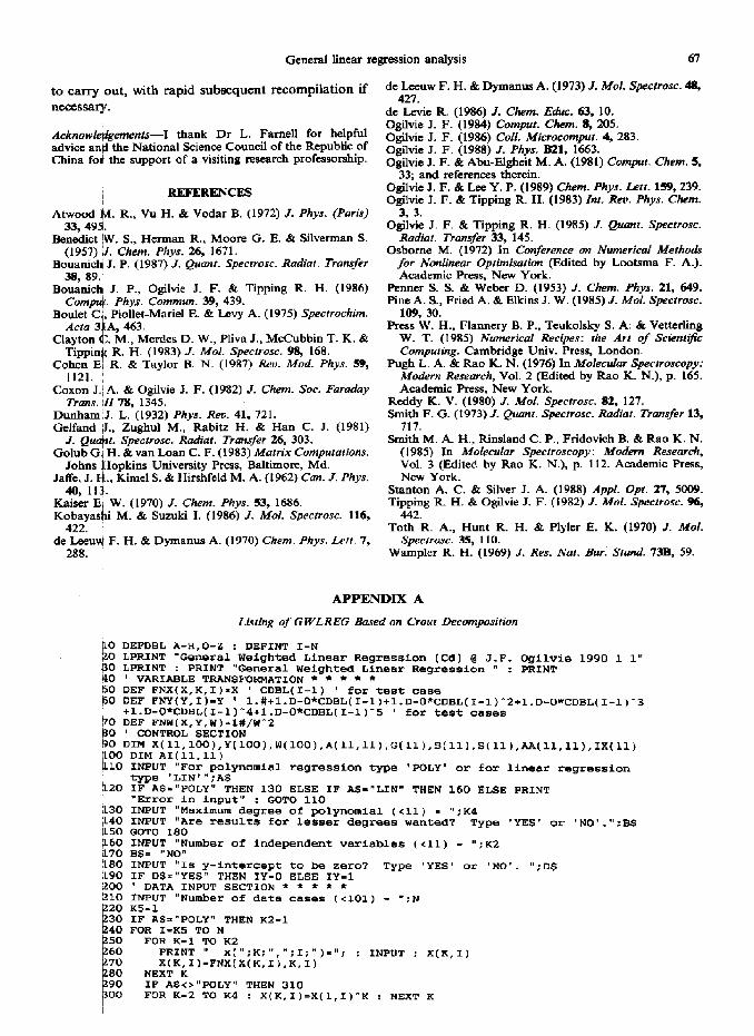
APPENDIX A

Listing of GWLREG Eased on Grout Decomposition

DEFDBL A-H,O-Z : DEFINT I-N LPRINT "General Weighted Linear Regression (Cd) @ J.F. Ogilvie 1990 1 1" LPRINT : PRINT 'General Weighted Linear Regression w : PRINT ’ VARIABLE TRANSFORMATION * * * * * DEF FNX(X,K,~)-x 0 cmL(I-1) 1 for test case DEF FNY(Y,I)-Y ’ 1.#+1.D-O*CDBL(I-1~+l.D-O*CDBL(~-l)-2+l.D-O*CDBL(I-l)-3 +1-D-O*CDBL(I-l)-Q+l.D-O*CDBL(I-11-5 ’ for test oases DEF FNW(X,Y,W)-l#/W'2 ’ CONTROL SECTION DIM X(ll,lOO),Y(lOO),W(loO).A(11,11~,G~ll),B(ll),S(ll~,~~ll,ll~,IX~ll~ DIM AI(ll.11) INPUT "For polynomial regreaSlOn type type 'LIN"';A$

'POLY' or for linear regression

IF A$="POLY" THEN 130 ELSE IF AS-"LIN" THEN 160 ELSE PRINT *Error in input" : GOT0 110 INPUT "Maximum degree of polynomial (~11) - ":K4 INPUT "Are results for lesser degrees wanted? Type 'YES' or 'NO'.":BS GOT0 180 INPUT "Number of independent variables (~11) = ":K2 B$= "No" INPUT "Is y-intercept to be zero? Type 'YES' or 'NO'. ":D$ IF DS="YES" THEN IY-0 ELSE IY-1 ’ DATA INPUT SECTION * * * * * INPUT "Number of data cases (~101) = ":N K5-1 IF AS=" POLY" THEN K2=1 FOR I-KS TO N

FOR K=l TO K2 PRINT II x(~':K:",":I;")I": : INPUT : X(K,I) X(K,I)-FNX(X(K.I),K,I)

NEXT K IF A$<>"POLY" THEN 310 FOR K-2 TO K4 : X(K,I)=X(l,I)-K : NEXT K

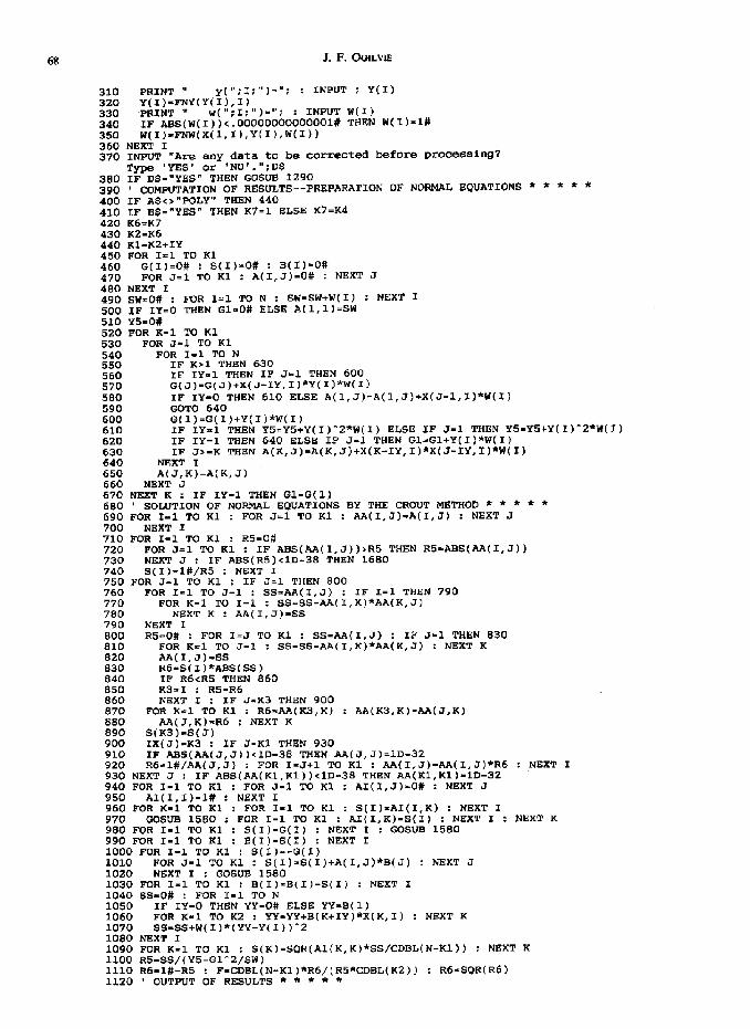
68 J. F. OOILVIE

PRINT u y(";I;")=": : INPUT ; Y(1) Y(I)-FNY(Y(I),I) PRINT n w(";I:")="; : INPUT W(I) IF ASS(W(I))<.~O~O~O~O~~O~~~# THEN W(I W(I)=FNW(X(l,I).Y(I).W(I))

310 320 330 340 350 360 370

300 390 400 410 420 430 440

NEXT I INPUT "Are mw data to be corrected befo Ire processing?

)=l#

&pe ‘YES’ or- 'NO'.";DS IF DS="YES" THEN WSUB I290 ' COMPOTATION OF RESULTS--PREPARATION OF NORMAL EQUATIONS * * * * * IF A$<>"POLY" THEN 440 IF B$="YBS" THEN K7=1 ELSE K?=K4 K6=K7 K2=K6 Kl-K2+IY FOR I=1 TO Kl 450

460 G(I)=O# : S(I)-O# : B(I)=O# 470 FOR J=l TO Kl : A(I,J)=O# : NEXT J 480 NEXT I 490 SW=O# : FOR 1~1 TO N : SW=SW+W(I) : NEXT I 500 IF IY=0 THEN Gl=O# ELSE A(l,l)=SW 510 Y5=0# 520 FOR K-l TO Kl 530 FOR J-1 TO Kl 540 FOR I-1 TO N 550 IF K>l THEN 630 560 IF IY-1 THEN IF J=l THEN 600 570 G(J)=G(J)+X(J-IY,I)*Y(I)*w(I) 580 IF IY-0 THEN 610 ELSE A(l,J)-A(l,J)+X(J-l,r)*W(I) 590 WTO 640 600 G(l)=G(I)+Y(I)*W(I) 610 IF IY=l THEN YS=YS+Y(I)-Z*W(I) ELSE IF J-1 THEN Y5.Y5+Y(I)-2*W(I) 620 IF IY=l THEN 640 ELSE IF J=l THEN Gl-Gl+Y(I)*W(I) 630 IF J>=K THEN A(K,J)-A(K,J)+X(K-IY,I)*X(J-IY,I)*W(I) 640 NEXT I 650 A( J,K)=A(K,J) 660 NEXT J 670 NEXT K : IF IY-l THEN Gl-G(1) 680 ' SOLUTION OF NORMAL EQUATIONS BY THE CROUT METHOD * * * * * 690 FOR I-1 TO Kl : FOR J=l TO K1 : AA(I,J)*A(I,J) : NEXT J 700 NEXT I 710 FOR 1-l TO Kl : R5=0# 720 FOR J-1 TO Kl : IF ABS(AA(I,J))>R5 THEN RS=ABS(AA(I, 51) 730 NEXT J : IF ABS(R5)<1D-38 THEN 1680 740 S(I).=l#/RJ : NEXT I 750 FOR J-1 TO Kl : IF J=l THEN 800 760 FOR I=1 TO J-l : SS=AA(I,J) : IF I=1 THEN 790 770 FOR K=l TO I-l : SS-SS-AA(I,K)*AA(K,J) 780 NBXT K : AA(I,J)-SS 790 NEXT I 800 R5-O# : FOR I=J TO Kl : SS-AA(1.J) : IF J-1 THEN 830 al0 FOR K=l TO J-l : SS-SS-AA(I,K)*AA(K,J) : NEXT K 020 AA(1, J)-SS a30 R6*S(I)*ABS(SS) a40 IF R6cR5 THEN 860 a50 K3-I : R5-R6 860 NEXT I : IF J-K3 THEN 900 am FOR K-1 TO Kl : R6=AA(K3,K) : AA(K3,K)-AA(J,K) a80 AA( J,K)-R6 : NEXT K 890 S(KB)d(J) 900 IX(J)-K3 : IF J-K1 THEN 930 910 IF ABS(AA(J,J))<ID-38 THEN AA(J,J)=lD-32 920 R6*1#/AA(J,J) : FOR T-J+1 TO Kl : AA(I,J)-AA(I,J)*R6 : NEXT I 930 NEXT J : IF ABS(AA(Kl,Kl))<lD-38 THEN AA(Kl,Kl)=lD-32 940 FOR I-l TO Kl : FOR J-l TO Kl : AI(I,J)-O# : NEXT J 950 AI(I,I)-l# : NEXT I 960 FOR K-1 TO Kl : FOR I-1 TO Kl : S(I)=AI(I,K) : NEXT I 970 GOSUB 1580 : FOR I-l TO K1 : AI(I,K)-S(1) : NEXT I : NEXT K 980 FOR I=1 TO Kl : $(1)-G(I) : NEXT I : GOSUB 1560 990 FOR I=1 TO Kl : B(l)-S(I) : NEXT I 1000 FOR I-l TO Kl : S(I)--G(I) 1010 FOR J=l TO Kl : S(I)-S(I)+A(I,J)*B( J) : NEXT J 1020 NEXT I : GOSUB 1580 1030 FOR I-l TO Kl : B(I)=B(I)-S(1) : NEXT I 1040 ss-O# : FOR I-l TO N 1050 IF IY-0 THEN YY-O# ELSE YY=B(l) 1060 FOR K=l TO K2 : YY=YY+B(K+IY)*X(K,I) : NEXT K 1070 ss-ss+W(I)*(YY-Y(I))"2 1080 NEXT I 1090 FOR K-1 TO Kl : S(K)=SOR(AI(K,K)*SS/CDBL(N-Kl)) : NEXT K 1100 R5-SS/(Y5-Gl-2/SW) 1110 R6=1#-R5 : F=CDBL(N-Kl)*Rs/(Rs+CDBL(K2)) : R6=SOR(R6) 1120 ’ OUTPUT OF RESULTS * * * * *

General linear regression analysis 69

1130 1140 1 50 i

;I% liS0 1 90 3! 1 00

1 10 t 1;20

1130 k 1 40

1250 lE60 1270 1280 lE90 1;300 1910 1:320 1[330 1340 x350 11360 11370 lt380 11390 1;aoo 1,410 I420 3430 11440 1450 1460 1470 1400 1490 1500 1510 s520 1530 1540

LPRINT : IF A$="POLY" THEN LPRINT "Degree of polynomial - ":K6 : LPRINT LPRINT “NO. Coefficient Standard Error" FOR K-l TO Kl : LPRINT K-IY,B(K),S(K) : NEXT K LPKTm 8 LPRINT “IF’-value I II, t LPRINW UEIN! "ww.##w#'- - - n IF8 LPRINT " Standard deviation of fit = * LPRINT USING "##.####-"--": SQR(SS*CDBL(N)/(kDBL(N-Kl)*SW)) LPRINT "Absolute value of sample Correlation Coefficient = ": R6 INPUT "Is table Of residuals wanted? Type 'YES ’ or ‘NO’.“:C$ IF C$-"YES" THEN GOSUB 1450 INPUT "Is table of correlation coefficients wanted? Type 'YES' or 'NO'.";CS IF CS-"YES" THEN GOSUB 1530 GOSUB 1290 IF A$<>"POLY" THEN 1700 K6-K6+1 IF K6<-K4 THEN 430 ELSE 1700 ’ DATA CORRECTION SECTION * * * * * PRINT : INPUT "Number of data oases to be deleted = ":K7 IF K7<1 THEN 1400 ELSE IF K7=1 THEN 1320 PRINT "Enter case numbers in descending Order." FOR J-l TO K7

N=N-1 INPUT "Case number to be deleted = ";K3 FOR I-K3 TO N

FOR K-1 TO X2 : X(K,I)=X(K,I+l) : NEXT K Y(I)=Y(I+l) : W(I)-w(I+l)

NEXT I NEXT J INPUT "Number of data cases to be added = “:K3 K5-N+l : N=N+K3 IF K7>0 OR K3>0 THEN 230 RETURN v OUTPUT OF TABLE OF RESIDUALS * * * * * LPRINT : LPRINT m Table of Residuals " : LPRINT LPRINT "Case No. X Y talc Y ohs Ycalc-Yobs FOR I=1 TO N

IF IY-0 THEN vV=O# ELSE YY=B(l) FOR K=l TO K2 : YY=YY+B(K+IY)*X(K,I) : NEXT K LPRINT " 1. ; I ; II ";X(l,I);" ";Yy; II ";Y(I):" ";YY-Y(1)

NEXT I LPRINT : RETURN ' OUTPUT OF COVARIANCE (CORRELATION) COEFFICIENTS * * * * * LPRINT n Parameter Correlation Matrix " : LPRINT FOR I=1 TO Kl : FOR Y=l TO I

LPRINT USING "###.####":AI(I.J)/SQR(AI(I,I)*AI(J,J)): 11550 Ii560 2570 NEXT J : LPRINT : NEXT I : RETURN 1560 ’ SUBSTITUTION SUBROUTINE * * * * * I590 K5-0 : FOR I=1 TO Kl : KB=IX(I) : SS-S(K3) I600 S(K3)=S(I) : IF K5=0 THEN 1620 1610 FOR J=K5 TO I-l : SS=SS-AA(I,J)*S(J) : NEXT J : GOT0 1630 1262; IF ABS(SS)>~D-36 THEN K5=1

S(I)=SS : NEXT I 4640 FOR I-K1 TO 1 STEP -1 : SS=S(I) 1650 1660 1670 4680

j% 1710 1720

IF I=Kl THEN 1670 FOR J=I+l TO Kl : SS-SS-AA(I,J)*S(J) : NEXT J S(I)-SS/AA(I,I) : NEXT I : RETURN

PRINT “Siingular matrix -- inversion aborted" ’ TERMINATION * * * * * LPRINT : PRINT : PRINT "Analysis completed" DS-INKEYS : IF DS-"" THEN 1710 END

:oo 30 LO

::

70

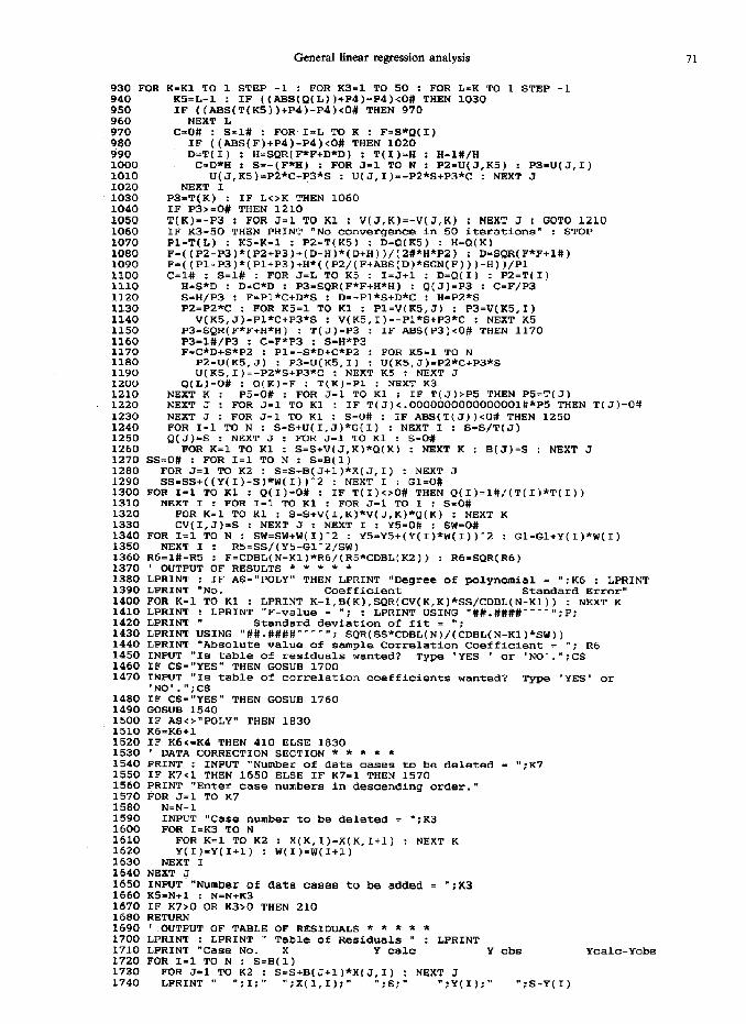
APPENDIX B

Listing of G WLREG Bclced on Singular-value Decomposition

DBFDBL A-H,O-Z : DEFINT I-N LPRINT “General Weighted Linear Regrsssion (svd) @ t.F. OgiIvie 1990 LPRINT : PRINT "General weighted Linear Regression : PRINT ’ VARIABLE TRANSFORMATION * * * * * DEF FNX(X,K,I)=X ' CDBL(I-1) ' for test Case DEF FNY(Y,I)-Y ' l.#+l.D-O*CDBL(I-l)+l.D-O*CDBL(I-1)-2+1.D-O*CDBL(I- +l.D-O*CDBL(I-l)-4+1.D-O*CDBL(I-l)-5 ' for teat Case8 DEF FNw(X,Y.W)-l#/W

1 1"

1)_3

80 ' CONTROL. SBCTION 90 DIM x(ll,lOO),~(lOO),w(lOO),~(lOO,ll),G(lOO),B(ll),CV(ll,ll)~T(l~) 100 DIM V(11,11).0(11) 110 INPUT “For polynomial regression type 'POLY' or for linear regression

type 'LIN"';A$

70 J. F. OGILVZ

120 IF AS-"POLY" THEN 130 ELSE IF AS="LIN" THEN 160 ELSE PRINT "Error in input" : GOT0 110

I.30 INPUT "Maximum degree of polynomial (tll) = ";K4 140 INPUT "Are results for lesser degrees wanted? Type 'YES' or 'NO'.":B$ 150 GOT0 180 160 INPUT "Number of independent variables (<ll) = ";K2 170 BS= "NO" 180 ' DATA INPUT SECTION * * * * * 190 INPUT "Number of data cases (~101) = ":N 200 K5=1 210 IF AS-"POLY" THEN K2=1 220 FOR I-K5 TO N 230 FOR K-l TO K2 240 PRINT ' x(":K;",";I;")="; : INPUT ; X(K,I) 250 X(K,I)-FNX(X(K,I),K,I) 260 NEXT K 270 IF A$<r"POLY" THEN 290 280 FOR K-2 TO K4 : X(K,I)=X(l,I)'K : NEXT K 290 PRINT 11 y(":I:")-": : INPUT : Y(1) 300 Y(I)=FNY(Y(I),I) 310 PRINT II w(";I;")=.'; : INPUT W(I) 320 IF ABS(W(1))<.00000000000001# THEN W(I)=l# 330 W(I)-FNW(X(1,I).Y(I),W(I)) 340 NEXT I 350 INPUT “Are any data to be corrected before processing? TYPO 'YES' or

'NO'.";D$ 360 IF DS=*YES" THEN GOSUB 1540 370 ' COMPUTATION OF RESULTS--PREPARATION OF DESIGN MATRIX * * * * * 380 IF A$<?"POLY' THEN 420 390 IF B$="YES" THEN K7=1 ELSE K7=Kd 400 K6=K7 410 KZ=K6 420 Kl=K2+1 430 FOR I=1 TO N 440 FOR J-1 TO K2 : U(I,J+l)-X(J,I)*W(I) : NEXT J 450 U(I.l)=W(I) : G(I)=Y(I)*W(I) : NEXT I 460 ' COMPUTATION OF RESULTS--SOLUTION BY SINGULAR-VALUE DECOMPOSITION * * 470 D=O# : P5=0# : P4.0# 480 FOR I-l TO Kl : L-I+1 : Q(I)=P5*D : D=O# : S=O# : P5-O# 490 IF I>N THEN 590 500 FOR K-I TO N : PS-PS+ABS(U(K,I)) : NEXT K 510 IF ABS(P5)<0# THEN 590 520 FOR K=I TO N : U(K,I)=U(K,I)/P5 : S.S+U(K,I)*U(K,I) : NEXT K 530 F-U(I,I) : D--SOR(S)*SGN(F) : H-Fell-S : U(I,I)=F-D 540 IF I-K1 THEN 580 550 FOR J.=L TO Kl : S=O# 560 FOR K-1 TO N : S.S+U(K,I)*U(K,J) t NEXT K 4 F-S/H 570 FOR K-I TO N : U(K,J)-U(K,J)+F*U(K,I) : NEXT K : NEXT J 580 FOR K=I TO N : U(K,X).P5*U(K,I) : NEXT K 590 T(I)=PS*D : D-0# : S=O# : P5-0# 600 IF I>N THEN 720 610 IF I-K1 THEN 720 620 FOR K=L TO Kl : PS=PS+ABS(U(I,K)) : NEXT K 630 IF ABS(P5)<0# THEN 720 640 FOR K-L TO Kl : U(I,K).U(I,K)/PS : S=S+U(I,K)*U(I,K) : NEXT K 650 F=V(I,L) : D=-SQR(S)*SGN(F) : H-F*D-S : U(I,L)=F-D 660 FOR K-L TO Kl : Q(K)-U(I,K)/H : NEXT K 670 IF I-N THEN 710 680 FOR J-L TO N : S=O# 690 FOR K-L TO Kl : S-S+U(J,K)*U(I,K) : NEXT K 700 FOR K=L TO Kl : U(J,K)=U(J,K)+S*Q(K) : NEXT K : NEXT J 710 FOR K-L TO Kl : U(I,K)-PS"U(1.K) : NEXT K 720 SEABS(T(I))+ABS(Q(I)) : IF Pd<S THEN P4-S 730 NEXT I 740 FOR I-K1 TO I STEP -1 : IF I>=Kl THEN 810 750 IF ABS(D)<O# THEN 800 760 FOR J=L TO Kl : V(J,I)-(U(I,J)/U(I,L))/D : NEXT 3 770 FOR J=L TO Kl : S-O# 780 FOR K-L TO Kl : S-S+U(I,K)*V(K,J) i NEXT K 790 FOR K-L TO Kl : V(K,J)-V(K,J)+S*V(K,I) : NEXT K : NEXT 2' 800 FOR Y-L TO Kl : V( I,J)=O# : V( J,I)-O# : NEXT J 810 V(I,I)-l# : D-Q(I) : L=I : NEXT I 820 FOR IrKl TO 1 STEP -1 : L-I+1 : D-T(I) 830 IF I<Kl THEN FOR J-L TO Kl : U(I,J)-O# : NEXT J 840 IF ABS(D)<O# THEN 910 050 D-l/%/D : IF I=Kl THEN 900 860 FOR J-L TO Kl : S=O# 070 FOR K=L TO N : S-S+U(K,I)*U(K,J) : NEXT K 080 F=(S/U(I,I))*D 090 FOR K-I TO N : tJ(K,J)=LJ(K,J)+F*U(K,I) : NEXT K : NEXT J 900 FOR J-1 TO N : U(J,I)PU(J,I)*D : NEXT J : GOT0 920 910 FOR J-I TO N : U(J,I).O# : NEXT J 920 U(I,I)-U(I,I)+l# : NEXT I

General linear regression analysis

930 FOR K-K1 TO 1 STEP -1 : FOR K3.1 TO 50 : FOR L=K TO 1 STEP -1

71

940 950 960 970 980 990 1000 1010 1020 1030 1040 1050 1060 1070 1080 1090 1100 1110 1120 1130 1140 1150 1160 1170 1180 1190 1200 1210 1220 1230 1240 1250 1260 1270 1280 1290 1300 1310 1320 1330 1340 1350 1360 1370 1380 1390 1400 1410 1420 1430 1440 1450 1460 1470

1480 1490 1500 1510 1520 1530 1540 1550 1560 1570 1580 1590 1600 1610 1620 1630 1640 1650 1660 1670 1680 1690 1700 1710 1720 1730 1740

K5=L-1 : IF ((ABS(Q(L))+PS)-P4)<0# THEN 1030 IF ((ABS(T(KS))+P4)-P4)<0# THEN 970

NEXT L C=O# : S=l# : FOR 1-L TO K : F=S*Q(I)

IF ((ABS(F)+P4)-P4)<0# THEN 1020 D-T(I) : H=SQR(F*F+D*D) : T(I)-H : H=l#/H C=D*H : SW-(F*H) : FOR J-l TO N : P2=U(J,K5) : P3=U(J,I)

U(J,K5)=P2*C+q3*S : U(J,I)--P2*S+P3*C : NEXT J NEXT I

PB=T(K) : IF L<>K THEN 1060 IF P3>=0# THEN 1210 T(K)--P3 : FOR J-l TO Kl : V(J,K)=-V(J,K) : NEXT J : GOT0 1210 IF X3-50 THEN PRINT "No convergence in 50 iterations" : STOP Pl=T(L) : K5-K-1 : P2-T(K5) : D-P(K5) : H-0(K) F=((P2-P3)*(P2+P3)+(D-H))/(2#fH*P2) : D=SQR(F*F+l#) F=((Pl-P3)*(Pl+P3)+H*((P2/(F+ABS(D)*SGN(F)))-H))/Pl C=l# : S=l# : FOR J=L TO K5 : I=J+l : D=Q(I) : P2=T(I)

H=S*D : D=C*D : P3=SQR(F*F+H*H) : Q(J)=PB : C-F/P3 S=H/P3 : F=Pl*C+D*S : D=-Pl*S+D*C : R=P2*S Pz=P2*c : FOR K5=1 TO Kl : Pl=V(KJ,J) : P3=V(K5,1)

V(K5,J)-Pl*C+P3*S : V(KS,I)=-Pl*S+P3*C : NEXT K5 P3=SQR(F*F+H*H) : T(J)=P3 : IF ABS(P3)<0# TREN 1170 P3=1#/P3 : C=F*P3 : S=H*P3 F-C*D+S*P2 : Pl--S*D+C*PZ : FOR K5-1 TO N

P2-U(K5.J) : P3=U(K5,1) : U(KS,J)-P2*C+P3*S U(K5,1)=-PZ*S+P3*C : NEXT K5 : NEXT J

Q(L)=O# : Q(K)=F : T(K)=Pl : NEXT K3 NEXT K : P5=0# : FOR J=l TO Kl : IF T(J)>P5 THEN P5=T(J) NEXT J : FOR J-1 TO Kl : IF T(J)<.00000000000OO0Ol#*P5 THEN T(J)=O# NEXT J : FOR J-l TO Kl : S=O# : IF ABS(T(J))<O# THEN 1250 FOR I=1 TO N : S=S+U(I,J)*G(I) : NEXT 1 : S-S/T(J) Q(J)& : NEXT J : FOR J=l TO Kl : S=O#

FOR K=l TO Kl : S=S+V(J,K)*Q(K) : NEXT K : B(J)=S : NEXT J SS=O# : FOR I=1 TO N : S-B(l)

FOR J=l TO K2 : S=SrB(J+l)*X(J,I) : NEXT J SS-SS+((Y(I)-S)*W(I))-2 : NEXT I : Gl=O#

FOR I-1 TO K1 : Q(I)=O# : IF T(I)<>O# THEN Q(I)=l#/(T(I)*T(I)) NEXT I : FOR I-1 TO Kl : FOR J=l TO I : S=O#

FOR K=l TO Kl : S=S+V(I,K)*V(J,K)*Q(K) : NEXT K CV(I,J)=S : NEXT J : NEXT I : Y5=0# : SW=O#

FOR I=1 TO N : SW=SW+W(I)_2 : Y5-Y5+(Y(I)*W(I))-2 : Gl=Gl+Y(I)*W(I) NEXT I : R5=SS/(Y5-Gl-Z/SW)

R6-l#-R5 : F=CDBL(N_Kl)*R6/(R5*CDBL(K2)) : R6=SQR(R6) ’ OUTPUT OF RESULTS * * * * * LPRINT : IF A$="POLY" THEN LPRINT "Degree of polynomial = ":K6 : LPRINT LPRINT "No. Coefficient Standard Error" FOR K=l TO Kl : LPRINT K-l,B(K),SQR(CV(K,K)*SS/CDBL(N-Kl)) : NEXT K LPRINT : LPRINT "F-value = ". : LPRINT USING "##.####----":F: LPRINT " Standard davktion of fit = ": LPRINT USING "##.####"""""; SQR(SS*CDBL(N),'(CDBL(N-Kl)*SW)) LPRINT "Absolute value of sample Correlation Coefficient = ": R6 INPUT "Is table of residuals wanted? Type 'YES ’ or ‘NO’.“;C$ IF CS-"YES" THEN GOSUB 1700 INPUT "Is table of correlation coefficients wanted? Type 'YES' or 'NO'.";CS IF C$="YES" THEN GOSUB 1760 GOSUB 1540 IF A$<>"POLY" THEN 1830 K6=K6+1 IF K6c=K4 THEN 410 ELSE 1830 ’ DATA CORRECTION SECTION * * * * * PRINT : INPUT "Number of data cases to be deleted = ":K7 IF K711 THEN 1650 ELSE IF K7=1 THEN 1570 PRINT "Enter case numbers in descending order." FOR J=l TO K7

N=N-1 INPUT "Case number to be deleted = ":K3 FOR I=K3 TO N

FOR K-l TO K2 : X(K,I)-X(K,I+l) : NEXT K Y(I)=Y(I+l) : W(I)=W(I+l)

NEXT I NEXT J INPUT "Number of date cases to be added = ";K3 K5-N+l : N=N+K3 IF K7>0 OR K3>0 THEN 210 RETURN 1 OUTPUT OF TABLE OF RESIDUALS * * * * * LPRINT : LPRINT 'I Table Of Residuals ' : LPRINT LPRINT "Case No. X Y talc Y obs FOR I=1 TO N : S=B(l)

FOR J=l TO K2 : S=S+B(J+l)*X(J,I) : NEXT J LPRINT " 0, ; I ; 1. ":X(1,1);" .I ; S ; II ":Y(I);" ":S-Y(1)

Ycalc-Yobs

72 J. F. 001~~~

1750 NEXT I : LPRINT : RETURN 1760 * OUTPUT 0~ COVARIANCE (CORRELATION) COEFFICIENTS * * * * * 1770 LPRINT * Parameter Correlation Matrix ' : LPRINT 1780 FOR I-l TO Kl : FOR J-l TO I 1790 LPRINT WPfNO “##U.#YI#“;CVLI. J)/SOR(CV(I,I)*CV(J,J))r 1800 NEXT J : LPRINT : NEXT I : RETURN 1810 PRINT “Singular matrix -- inversion aborted" 1820 ' TERMINATION * * * * * 1630 LPRINT : PRINT : PRINT "Analysis completed" 1840 DS-INKEYS : IF D$="" THEN 1840 1850 END