1. INTRODUCTIONCommission Internationale de l’Eclairage (CIE) has forsome time been active in developing a new physiologicallybased system for colorimetry.1 This attempt rests on theidea that there exists a linear relationship between colormatching functions (CMF’s) and the fundamental re-sponse curves of three types of photoreceptormechanisms—the physiological fundamentals.2 In thisrespect, the fundamentals can be regarded as a specialrepresentation of CMF’s. Psychophysical experimentsperformed over the past 50 years show that no such con-nection can be made with satisfactory precision on the ba-sis of the current CIE1931 standard colorimetricobserver.3,4
The technical committee CIE TC 1-36 has consideredusing the Stiles–Burch1959 10° observer5 (with some mi-nor modifications) as its colorimetric database, becausethese data represent a body of solid experimental mate-rial based exclusively on color matching. With this basisone would like to derive, for the 2° and 10° visual fields, afundamental tristimulus space accompanied by (1) a chro-maticity diagram obtained by a conical projection of thepoints of this space and (2) an equiluminant chromaticitydiagram constructed along the lines of Luther6 andMacLeod and Boynton.7,8 However, it is also desirable toestablish a connection to the existing CIE1931 XYZ system,particularly for any set of 2° CMF’s that may be derivedfrom the (slightly modified) Stiles–Burch1959 10°observer.9 Here we will present a general and detailedaccount of how to design an XYZ representation given anyset of CMF’s. This exercise is useful for two main rea-sons. First, it has given us the opportunity to review theprinciples behind the CIE1931 colorimetric system. Thisreview has revealed some arbitrariness in the criteria
used. Second, since practically all exact color specifica-tions are given in terms of chromaticity coordinates, itwould be advantageous to make possible comparisons ofchromaticity coordinates of identical stimuli in diagramsthat differ minimally.
In the course of this work, we discovered that not allthe criteria defining the CIE1931 XYZ tristimulus spacewere explicitly stated. Some conditions were hard totrace in the literature, and one of these, in particular, wasrather loosely formulated. In a recapitulation of the con-siderations that led to the CIE1931 XYZ system, we willpresent the old criteria used by CIE and also introducesome additional constraints to replace the more impreciseoriginal formulations.
In our presentation we will use, as an example, the de-velopment of an XYZ representation of the CMF’s of theStiles–Burch1955 2° pilot group.10 We denote this newrepresentation the X–Y–Z– tristimulus space, and we re-fer to the corresponding chromaticity diagram as the(x–, y–) diagram. The diagram has already been used byus in a comparison of the chromaticity differences that re-sult from adopting different sets of physiologicalfundamentals.11
2. THE CIE XYZ CONCEPTA detailed outline of the considerations that led to thecurrent CIE1931 XYZ system can be found in the paper bySmith and Guild12 and in the review paper by Fairmanet al.13 The well-known main criteria may be listed asfollows:
1. All color stimuli are to have all nonnegative tri-stimulus values.
1999 Optical Society of America
2846 J. Opt. Soc. Am. A/Vol. 16, No. 12 /December 1999 J. H. Wold and A. Valberg
2. In the chromaticity diagram the alychne is to berepresented by a line coinciding with the abscissa axis.
3. The chromaticity coordinates of Illuminant E (theequal power spectrum) are to equal 1/3 each.
In principle, there are many ways to ensure that criterion1 is fulfilled.14,15 The procedure actually followed in de-veloping the CIE1931 standard was to choose the new (vir-tual) primaries X, Y, and Z so that, in the chromaticitydiagram of the CIE RGB (red–green–blue) representation(referring to physical primaries),16,17 their chromaticitypoints define the vertices of a triangle that fully circum-scribes the spectrum locus.12
Criterion 2 requires that two of the primaries be repre-sented on the alychne, with the consequence that theCMF referring to the remaining primary is proportionalto the adopted spectral luminous efficiency function.14,18
In CIE’s standard representation this proportionality be-tween the CMF y(l) and the CIE spectral luminous effi-ciency function for photopic vision19 is restricted to iden-tity: i.e., y(l) [ V(l).
Criterion 3 implies that the CMF’s must be normalizedso that their integrals over the spectrum are the same forall three functions.
Obviously, criteria 1–3 do not define a unique XYZ rep-resentation. In order for an unequivocal representationto be obtained, additional constraints are necessary. Inthe relevant publications these constraints concern thesides of the triangle that circumscribes the spectrum lo-cus in the RGB representation. For instance, regardingthe boundary connecting the chromaticity points of theprimaries X and Y—the side XY—Smith and Guildstated12:
The side XY of the color triangle [the circumscribingtriangle] is made to pass through R, the red terminusof the spectral locus.... To extend the number of zerocoordinates as far as possible, we make XY tangen-tial to the spectral locus at R.
Whereas the above criterion is quite precise, the condi-tions for determining the side YZ are less accurate12:
The conditions are that it [side YZ] should pass thespectral locus at a reasonable distance, and lie in adirection which give a favourable disposition of thespectral locus within the triangle.
3. CONCEPT OF THE NEW X–Y–Z–
TRISTIMULUS SPACEIn designing a new colorimetric XYZ system, one may dis-cuss which criteria are useful. In deriving an XYZ rep-resentation of the Stiles–Burch1955 2° pilot group, wehave made the decision to apply much the same principlesas those used in developing the CIE1931 standard, but tostate the requirements more precisely whenever neces-sary. We have preferred an exact mathematical method,based partly on geometrical considerations. It should beemphasized, however, that this approach is only one ofmany possible alternatives.
A vital point in our method regards the constraints im-posed on the side YZ of the circumscribing triangle, inwhich the Smith–Guild formulation above is replaced by
the requirement of minimum difference between the new(x–, y–) diagram and our chosen reference diagram,20–22
the Judd–Vos (x8, y8) diagram.23,24 Moreover, on the as-sumption that the S cone does not contribute toluminance,25–29 the spectral luminous efficiency functiondefining the alychne in X–Y–Z– space has been chosen toequal a linear combination of the 2° fundamental L and Mresponse curves (L and M fundamentals) given by Stock-man et al.30 We denote this synthesized spectral lumi-nous efficiency function V–(l).
Now, in order to comply with the CIE 1931 procedure,modified as outlined above, we propose that the mainsteps in developing the new Stiles–Burch1955 X–Y–Z– tri-stimulus space should be as follows:
1. Transform the Judd–Vos (x8, y8) diagram to an(r8, g8) diagram that (a) refers to Wright primaries R8,G8, and B8 representing monochromatic stimuli of wave-lengths 700.0, 546.1, and 435.8 nm, respectively, and (b)has Illuminant E represented at the point (rE8 , gE8 )5 ( 1
3, 13).
2. Transform the original Stiles–Burch1955 ( r–, g–)
diagram (referring to primaries R–, G–, and B– that rep-resent unit radiance, monochromatic stimuli with wavenumbers 15,500, 19,000, and 22,500 cm21, respectively)into an (r–, g–) diagram that (a) refers to Wright prima-
ries R–, G–, and B– that represent monochromaticstimuli of wavelengths 700.0, 546.1, and 435.8 nm, re-spectively, and (b) has Illuminant E represented at thepoint (rE
– , gE– ) 5 ( 1
3, 13).
3. In the (r–, g–) diagram choose the chromaticity
points for the new primaries X–, Y–, and Z– such that thefollowing criteria are fulfilled:
(i) The chromaticity points of the primaries X–, Y–
and Z– define the vertices of a triangle that fullycircumscribes the spectrum locus.
(ii) The boundary connecting the chromaticitypoints of the primaries X– and Z– (the side XZ)coincides with the line representing the alychneas defined relative to the synthesized V–(l).
(iii) The boundary connecting the chromaticitypoints of the primaries X– and Y– (the side XY)– has the same slope as the line connecting the
chromaticity points of the primaries X8 andY8 in the Judd–Vos (r8, g8) diagram.
– is tangent to the spectrum locus in the longwavelength region.
(iv) The shortest distance from the spectrum locusto the boundary connecting the chromaticitypoints of the primaries Y– and Z– (the side YZ)is equal to the corresponding distance in theJudd–Vos (r8, g8) diagram.
(v) When the above criteria are obeyed, the meanEuclidean difference between correspondingpoints on the spectrum loci in the new (x–, y–)diagram and the Judd-Vos (x8, y8) diagram isminimum according to a least-root-mean-square
J. H. Wold and A. Valberg Vol. 16, No. 12 /December 1999 /J. Opt. Soc. Am. A 2847
(RMS) criterion, calculated at 1-nm intervals.[This criterion determines the slope of the sideYZ in the (r–, g–) diagram.]
4. From the r– and g– coordinates of the primaries
X–, Y–, and Z–, derive a new (x–, y–) chromaticity dia-gram satisfying the criterion
(vi) Illuminant E is represented at the point(xE– , yE
–) 5 ( 13, 1
3).
5. Determine the CMFs x–(l), y–(l), and z–(l) un-der the constraint
(vii) y–(l) [ V–(l).
Criteria (i), (ii), and (vi), parallel CIE criteria 1, 2, and 3,respectively. Furthermore, criteria (iii), (iv), and (v) arethose that have been introduced to unequivocally definethe representation, thereby replacing the more impreciseformulations of Smith and Guild.12
The remaining criterion, (vii), ensures that the finalrepresentation is in conformity with CIE’s standard by re-quiring that the choice of a common scaling factor for theCMF’s make the CMF that refers to the Y primary iden-tical to the adopted spectral luminous efficiency function.
4. (r8, g8) CHROMATICITY DIAGRAM OFTHE JUDD–VOS MODIFIED 2°OBSERVERSince the Judd–Vos modified 2° observer23,24 is consid-ered a significant improvement of the CIE1931 standardcolorimetric observer,3,4 we decided to use the Judd–Vos(x8, y8) chromaticity diagram as a reference in our work.Furthermore, in order to follow as closely as possible theprocedure adopted by CIE, we regarded it as important torefer all geometric manipulations to a correspondingJudd–Vos (r8, g8) diagram. This diagram refers toWright primaries R8, G8, and B8 that represent mono-chromatic stimuli of wavelengths 700.0, 546.1, and 435.8nm, respectively, and has Illuminant E represented at thepoint (rE8 , gE8 ) 5 ( 1
3, 13). Since the Judd–Vos modified 2°
observer was obtained by simply adjusting the CIE1931CMF’s x(l), y(l), and z(l) directly, without reference
back to an RGB representation, no such (r8, g8) diagramwas ever published. Being relevant for the work at hand,this diagram therefore had to be derived separately.
The projective transformation Tx8r8 converting the chro-
maticity coordinates of the Judd–Vos XYZ representationinto chromaticity coordinates of a corresponding RGBrepresentation is given in symbolic terms in Appendix A,Eqs. (A1). On insertion of the appropriate numerical val-ues, selected from Table 1, and elimination of dependentcoordinates, the final transformation equations turn outto be
rQ8 54.532604xQ8 2 0.682602yQ8 2 0.758220
1.933206xQ8 2 0.165284yQ8 1 1,
gQ8 520.978903xQ8 1 2.169755yQ8 1 0.129175
1.933206xQ8 2 0.165284yQ8 1 1, (1)
with xQ8 and yQ8 denoting the chromaticity coordinates of astimulus Q in the Judd–Vos XYZ representation and rQ8and gQ8 the chromaticity coordinates in the new RGB rep-resentation.
Figure 1(a) shows the original Judd–Vos (x8, y8) dia-gram, and Fig. 1(b) shows the new (r8, g8) diagram.Both diagrams show (1) the chromaticity points (X8),(Y8), and (Z8) of the original primaries X8, Y8, and Z8; (2)the chromaticity points (R8), (G8), and (B8) of the newprimaries R8, G8, and B8; and (3) the chromaticity point(E) of Illuminant E. With respect to the latter, it shouldbe emphasized that the (x8, y8) diagram deviates fromideality in having the chromaticity point of Illuminant Eslightly displaced from (1
3, 13). The (r8, g8) diagram, how-
ever, is made ideal by placing the chromaticity point of Il-luminant E at exactly (1
3, 13). The coordinate values of the
chromaticity points displayed in the figures are given inTable 1.
Also drawn in Fig. 1(b) are the straight lines L18 , L28 ,and L38 connecting the chromaticity points (X8), (Y8), and(Z8) of the old primaries X8, Y8, and Z8. The inset dia-grams to the left and right show magnifications of the twolocus segments framed in the main plot. The ordinatesd18 and d38 of these blowups give the Euclidean distances
Table 1. Chromaticity Coordinates of the Reference Stimuli X8, Y8, Z8 and R8, G8, B8 As Well As of the CIEIlluminant E, in the Respective XYZ and RGB Representations of the Judd–Vos Modified 2° Observer
a Values obtained by interpolation of spectral chromaticity coordinate functions (see Ref. 34).b Values taken from Vos (Ref. 24).
2848 J. Opt. Soc. Am. A/Vol. 16, No. 12 /December 1999 J. H. Wold and A. Valberg
Fig. 1. (a) (x8, y8) chromaticity diagram of the Judd–Vos modified 2° observer. Filled circles on the spectrum locus mark the chro-maticity points (R8), (G8), and (B8) of the new Wright primaries. The chromaticity point (E) of Illuminant E is positioned at(xE8 , yE8 ) 5 (0.33499, 0.33618), i.e., slightly displaced from the ideal point (1/3, 1/3). (b) (r8, g8) chromaticity diagram of the Judd–Vosmodified 2° observer resulting from transformation Eqs. (1). The diagram refers to Wright primaries R8, G8, and B8 representingmonochromatic stimuli of wavelengths 700.0, 546.1, and 435.8 nm, normalized so that the chromaticity point (E) of Illuminant E ispositioned at (rE8 , gE8 ) 5 (1/3, 1/3). Lines L18 , L28 , and L38 (dashed) constitute a circumscribing triangle with vertices at the chromaticitypoints (X8), (Y8), and (Z8) of the old primaries. Ordinates d18 and d38 of the inset magnifications give the Euclidean distances betweenthe points on the locus segments (framed) and their respective closest points on the lines L18 and L38 . Point (D8) marks the locus pointof shortest distance to line L18 . Line L38 intersects the abscissa axis in point (P8).
J. H. Wold and A. Valberg Vol. 16, No. 12 /December 1999 /J. Opt. Soc. Am. A 2849
between the points on the locus segments and their re-spective closest points on the lines L18 and L38 .
Numerical analysis shows that the distance d1D88 be-
tween L18—the YZ side of the circumscribing triangle—and the locus point (D8) closest to the line is
d1D88 5 0.020365. (2)
The parameter value at (D8) turns out to be lD85 504.046 nm, and accordingly (D8) is given as(rD8
8 , gD88 ) 5 (21.308762, 1.681121).
Regarding the line L38 connecting the points (X8) and(Y8)—the XY side of the circumscribing triangle—itsslope a38 is
a38 5gY8
8 2 gX88
rY88 2 rX8
85 21.010269. (3)
In our development of an XYZ representation of theStiles–Burch1955 2° pilot group, the parameters d1D8
8 anda38 play a central role in that their values are adopted forthe corresponding parameters that unequivocally deter-mine the chromaticity coordinates of the new primariesX–, Y–, and Z– in a diagram analogous to the (r8, g8) dia-gram of Fig. 1(b).
5. (r–, g–) CHROMATICITY DIAGRAM OFTHE STILES-BURCH1955 2° PILOT GROUPThe original tabulations of the Stiles–Burch1955 2° pilotgroup10,31 are given in an RGB representation referringto primaries R–, G–, and B– that represent monochro-matic stimuli of unit radiance and wave numbers 15,500,19,000, and 22,500 cm21, respectively. Initially, there-
fore, in order to develop the XYZ representation in com-pliance with the CIE procedure, we transformed the( r–, g–) diagram of the RGB representation into an
(r–, g–) diagram analogous to the (r, g) diagram in theRGB representation of the CIE1931 standard colorimetricobserver.
The projective transformation Tr–r– that converts the
chromaticity coordinates of the Stiles–Burch RGB repre-sentation into chromaticity coordinates of a correspond-ing RGB representation is given in symbolic terms in Ap-pendix B, Eqs. (B1). After inserting the appropriatenumerical values, read from Table 2, and eliminating de-pendent coordinates, we reduce the transformation equa-tions to
rQ– 5
0.403966rQ– 2 0.217818gQ
– 2 0.016470
20.607510rQ– 2 0.635054gQ
– 1 1,
gQ– 5
20.003951rQ– 1 0.575889gQ
– 1 0.009406
20.607510rQ– 2 0.635054gQ
– 1 1, (4)
where rQ– and gQ
– denote the chromaticity coordinates of a
stimulus Q in the original RGB representation and rQ–
and gQ– denote the chromaticity coordinates in RGB rep-
resentation.Figure 2(a) shows the original ( r–, g–) chromaticity
diagram of the Stiles–Burch1955 2° pilot group, and Fig.2(b) shows the (r–, g–) diagram resulting from transfor-mation equations (4). In both diagrams are shown (1)the chromaticity points (R–), (G–), and (B–) of the origi-
nal primaries R–, G–, and B–; (2) the chromaticity points
(R–), (G–), and (B–) of the primaries R–, G–, and B–;
Table 2. Chromaticity Coordinates of the Reference Stimuli R–, G–, B–; R–, G–, B– and X–, Y–, Z– As WellAs of the CIE Illuminant E, in the Respective RGB, RGB, and XYZ Representations of the
E 0.579468b 0.265210b 0.155322b 1/3 1/3 1/3 1/3 1/3 1/3
a Values obtained by interpolation of spectral chromaticity coordinate functions (see Ref. 34).b Values obtained by integration of color matching functions (see Ref. 34).
2850 J. Opt. Soc. Am. A/Vol. 16, No. 12 /December 1999 J. H. Wold and A. Valberg
Fig. 2. (a) ( r–, g–) chromaticity diagram of the Stiles–Burch1955
2° pilot group. The diagram refers to primaries R–, G–, and B–
representing unit radiance, monochromatic stimuli with wavenumbers 15,500, 19,000, and 22,500 cm21. Filled circles on thespectrum locus mark the chromaticity points (R–), (G–), and
(B–) of the new Wright primaries. The chromaticity point (E) ofIlluminant E is positioned at ( rE
– , gE–) 5 (0.579468, 0.265210).
(b) (r–, g–) chromaticity diagram of the Stiles–Burch1955 2° pilotgroup resulting from transformation Eqs. (4). The diagram re-
fers to Wright primaries R–, G–, and B– representing mono-chromatic stimuli of wavelengths 700.0, 546.1, and 435.8 nm,normalized so that the chromaticity point (E) of Illuminant E ispositioned at (rE8 , gE8 ) 5 (1/3, 1/3). Filled squares on the spec-trum locus mark the chromaticity points (R–), (G–), and (B–) ofthe original Stiles–Burch primaries ( joined by dashed lines).
and (3) the chromaticity point (E) of Illuminant E. Thecorresponding numerical coordinate values are found inTable 2.
6. CIRCUMSCRIPTION OF THE SPECTRUMLOCUS IN THE (r–, g–) DIAGRAM
According to the concept of the X–Y–Z– tristimulus space,
in the corresponding (r–, g–) diagram the triangle with
vertices at the chromaticity points of the primaries X–,
Y–, and Z– must fully circumscribe the spectrum locus.The lines making up the triangle are denoted as follows:
• L1– is the line connecting the chromaticity points of
the primaries Y– and Z– (the YZ line);
• L2– is the line connecting the chromaticity points of
the primaries X– and Z– (the XZ line);
• L3– is the line connecting the chromaticity points of
the primaries X– and Y– (the XY line).
A. XZ Line, L2– (the Alychne Line)
The XZ line L2– connecting the chromaticity points of the
primaries X– and Z– was taken as the line representingthe alychne as defined by the synthesized spectral lumi-nous efficiency function V–(l). As already mentioned,this function equals a linear combination of the 2° L andM fundamentals of Stockman et al.30 Thus, if L–(l) and
M–(l) denote these fundamentals, we have
V–~l! 5 cLL–~l! 1 cMM–~l!. (5)
The functions L–(l) and M–(l) are given as linear com-binations of the CMF’s of the Stiles–Burch1955 2° pilotgroup; that is,
L–~l! 5 aL1 r–~l! 1 aL2 g–~l! 1 aL3b–
~l!,
M–~l! 5 aM1 r–~l! 1 aM2 g–~l! 1 aM3b–
~l!, (6)
with r–(l), g–(l), and b–
(l) denoting the CMF’s of theRGB representation. If we substitute L–(l) and M–(l)
into Eq. (5), the equation for V–(l) takes the form
V–~l! 5 ~cLaL1 1 cMaM1! r–~l!
1 ~cLaL2 1 cMaM2! g–~l!
1 ~cLaL3 1 cMaM3! b–
~l!. (7)
Since, by definition, the luminosities [as defined relativeto V–(l)] of the stimuli represented on the alychne [refer-
ring to V–(l)] are all zero, Eq. (7) implies that the line in
the original ( r–, g–) diagram representing this alychne(the alychne line) is given by the equation
J. H. Wold and A. Valberg Vol. 16, No. 12 /December 1999 /J. Opt. Soc. Am. A 2851
with r– and g– denoting the chromaticity coordinates in
RGB representation. The chromaticity coordinate, b–,
has been eliminated here by use of the relation b– 5 1
2 r– 2 g–.According to the paper of Stockman et al.,30 the values
of the coefficients aLi (i 5 1, 2, 3) and aMi (i 5 1, 2, 3)are
aL1 5 0.214808, aM1 5 0.022882,
aL2 5 0.751035, aM2 5 0.940534,
aL3 5 0.045156, aM3 5 0.076827. (9)
To further comply with the work of Stockman et al.,30 wedecided to adopt their proposals for the values of the co-efficients cL and cM as well; i.e.,32
cL 5 0.682882, cM 5 0.352429. (10)
Inserting the values of Eqs. (9) and (10) into Eq. (8) andsubstituting r i
– (i 5 1, 2, 3) by using the inverse of Eqs.(4), i.e., the transformation
r– 52.510421r– 1 0.984891 g– 1 0.032082
1.520274 r– 1 1.677748 g– 1 1,
g– 50.007609 r– 1 1.699724 g– 2 0.016113
1.520274 r– 1 1.677748 g– 1 1, (11)
we determine the equation of the alychne line L2– in the
new (r–, g–) diagram. (Since the above transformation isa mapping of a line, indices Q are dropped in the trans-formation variables.) The equation turns out to be
L2– : g– 5 a2
–r– 1 b2– , a2
– 5 20.212634,
b2– 5 20.031615. (12)
The line is shown in Fig. 3(a).
B. XY Line, L3–
In conformity with the CIE concept, the XY line wasdrawn tangential to the spectrum locus in the long-wavelength region. As the first step, a set of interpola-tion functions for the spectral chromaticity coordinates inthe RGB representation were determined. Then, with acontinuous parametric representation of the spectrum lo-cus in the (r–, g–) diagram at hand, a line of slope a3
–
equal to the slope of the corresponding line in the Judd-Vos (r8, g8) diagram, i.e.,
a3– 5 a38 5 21.010269, (13)
was made tangent to the spectrum locus at one singlepoint (T–). The resulting XY line, L3
– , is shown in Fig.3(a). The inset to the right shows a magnification of thelong-wavelength region of the spectrum locus. Here theordinate d3
– is the Euclidean distance between the pointson the locus segment and their respective closest points
on L3– . The blowup shows that compared with the XY
lines in the analogous Judd–Vos (r8, g8) and CIE1931
(r, g) diagrams, the line L3– is shifted slightly to the right.
This parallel shift is due to a small convexity in the long-wavelength region of the spectrum locus in the (r–, g–)diagram, a convexity not present in the other two dia-grams. An alternative procedure would have been tosmooth the color matching data of the red flank of thespectrum before drawing the tangent line. However, notknowing whether the convexity reflects some significantphysiological mechanism, such as rod intrusion33 or otherinfluences, we decided to keep the data unchanged.
By means of numerical calculations, the tangent point(T–) between the XY line L3
– and the spectrum locus is
determined to be (rT–– , gT–
– ) 5 (0.979429, 0.021946),which corresponds to the parameter value lT–
5 637.849 nm. Given that we know the value of a3– ,
this implies that the equation of the chosen XY line is
L3–: g– 5 a3
–r– 1 b3– , a3
– 5 21.010269,
b3– 5 1.011432. (14)
The point (P–) of intersection between L3– and the ab-
scissa axis turns out to be (rP–– , gP–
– ) 5 (1.001152, 0). Incomparison, the corresponding points in the Judd–Vos(r8, g8) and CIE1931 (r, g) diagrams are (rP8
As already mentioned, the criteria imposed on the YZ lineare the following:
• The distance d1D–– from the YZ line’s closest point
(D–) on the spectrum locus is to equal the correspondingdistance in the Judd–Vos (r8, g8) diagram; that is,
d1D––
5 d1D88 5 0.020365. (15)
• The slope of the line is to be adjusted so that the ver-tices of the resulting circumscribing triangle define thechromaticity points of new primaries X–, Y–, and Z–, pro-
viding the basis for an (x–, y–) diagram whose spectrumlocus differs as little as possible from the spectrum locusin the Judd–Vos (x8, y8) diagram.
To be precise, the latter criterion requires that the Euclid-ean difference between the two spectrum loci be mini-mum according to a least-RMS criterion. Letting xl8 andyl8 denote the chromaticity coordinates of a monochro-matic stimulus of wavelength l in the Judd–Vos XYZ rep-resentation and xl
– and yl– the corresponding chromaticity
coordinates in the new Stiles–Burch XYZ representation,the RMS is interpreted as
RMS 5 H 1
341 (l5390
730
@~xl– 2 xl8 !2 1 ~ yl
– 2 yl8 !2#J 1/2
, (16)
with 341 5 730 2 390 1 1 being the number of tabu-lated values in the 1-nm tabulations of theStiles–Burch1955 2° pilot group.31 Numerical minimiza-tion shows that the RMS is minimum when the wave-
2852 J. Opt. Soc. Am. A/Vol. 16, No. 12 /December 1999 J. H. Wold and A. Valberg
Fig. 3. (a) (r–, g–) chromaticity diagram of the Stiles–Burch1955 2° pilot group [same as the diagram of Fig. 2(b)] with lines L1–, L2
– , and
L3– (dashed) constituting a circumscribing triangle with vertices at the chromaticity points (X–), (Y–), and (Z–) of the new primaries
X–, Y–, and Z–. Ordinates d1– and d3
– of the inset magnifications give the Euclidean distances between the points on the locus seg-
ments (framed) and their respective closest points on the lines L1– and L3
– . Point (D–) marks the locus point of shortest distance to line
L1– . Line L3
– is tangent to the spectrum locus in point (T–) and intersects the abscissa axis in (P–). (b) (x–, y–) chromaticity diagramof the Stiles–Burch1955 2° pilot group resulting from transformation Eqs. (19). Filled circles on the spectrum locus mark the chroma-ticity points (R–), (G–), and (B–) of the Wright primaries underlying the (r–, g–) diagram. The chromaticity point (E) of Illuminant
E is positioned at (xE– , yE
–) 5 (1/3, 1/3).
J. H. Wold and A. Valberg Vol. 16, No. 12 /December 1999 /J. Opt. Soc. Am. A 2853
length parameter at the point (D–) on the spectrum locus
of shortest distance d1D–– to the YZ line is lD–,min
5 501.662 nm, implying that (D–) is given as
(rD–– , gD–
– ) 5 (21.398789, 1.788181). The correspondingleast-RMS value is RMSmin 5 0.021411. Further detailson the computations involved are given elsewhere.34
Once the wavelength parameter lD–,min is determined,the coefficients determining the optimized YZ lineL1–—i.e., the slope a1
– and the ordinate b1– of intersection
with the ordinate axis—can be calculated, yielding thefollowing equation for L1
– :
L1– : g– 5 a1
–r– 1 b1– , a1
– 5 22.629242,
b1– 5 21.946861. (17)
The line is shown in Fig. 3(a). In the inset to the left,showing a magnification of the spectrum locus in the vi-cinity of (D–), the ordinate d1
– is the Euclidean distancebetween the points on the locus segment and their respec-tive closest points on L1
– .
D. Optimized Circumscribing TriangleGiven that the equations of the lines L1
– , L2– , and L3
– con-stituting the optimized circumscribing triangle areknown, the coordinates of its vertices—i.e., the chromatic-ity coordinates of the new primaries X–, Y–, and Z–—aregiven by the equations
rX––
5b3– 2 b2
–
a2– 2 a3
–, gX–
–
5a2–b3– 2 a3
–b2–
a2– 2 a3
–,
rY––
5b1– 2 b3
–
a3– 2 a1
–, gY–
–
5a3–b1– 2 a1
–b3–
a3– 2 a1
–,
rZ––
5b2– 2 b1
–
a1– 2 a2
–, gZ–
–
5a1–b2– 2 a2
–b1–
a1– 2 a2
–. (18)
The numerical values, obtained by inserting the coeffi-cients from Eqs. (12), (14), and (17), are listed in Table 2.
Since the vertices of the circumscribing triangle definethe chromaticity points of the new primaries, they are la-beled (X–), (Y–), and (Z–) in Fig. 3(a).
7. XYZ REPRESENTATION OF THESTILES–BURCH1955 2° PILOT GROUPWith the circumscribing triangle thus established, thederivation of the (x–, y–) diagram is now straightforward.The projective transformation T r–
x– converting chromatic-ity coordinates from RGB to XYZ representation is givenin symbolic terms in Appendix B, Eqs. (B2). By insertionof the appropriate values, read from Table 2, and elimi-nation of dependent coordinates, the equations trans-forming from chromaticity coordinates rQ
– and gQ– to new
coordinates xQ– and yQ
– are determined to be
xQ– 5
0.228051rQ– 1 0.086736gQ
– 1 0.168864
20.448711rQ– 2 0.087153gQ
– 1 1,
yQ– 5
0.133580rQ– 1 0.628216gQ
– 1 0.019861
20.448711rQ– 2 0.087153gQ
– 1 1. (19)
As seen from Table 2, in the (x–, y–) diagram deter-mined by Eqs. (19), the CIE Illuminant E is representedat exactly ( 1
3, 13). The corresponding chromaticity point
in the Judd–Vos (x8, y8) diagram is (0.33499, 0.33618).24
The concept of the circumscription of the spectrum lo-cus in the (r–, g–) diagram is sketched in Fig. 3(a), and
the (x–, y–) diagram resulting from transformation Eqs.(19) is shown in Fig. 3(b). Plotted in both diagrams are(1) the chromaticity points (R–), (G–), and (B–) of the
Wright primaries R–, G–, and B–; (2) the chromaticity
points (X–), (Y–), and (Z–) of the new primaries X–, Y–,
and Z–; and (3) the chromaticity point (E) of IlluminantE. The numerical values of the corresponding chromatic-ity coordinates are given in Table 2.
Now that the new (x–, y–) diagram has been created
with the help of an intermediate (r–, g–) diagram, whatremains is to determine the direct-route transformationof chromaticity coordinates from the Stiles–Burch origi-nal RGB representation into the new XYZ representa-tion. Clearly, we can do this by substituting rQ
– and gQ–
into Eqs. (19), using transformation equations (4). Moredirectly, however, the composite transformation isachieved by inserting the appropriate values—taken fromTable 2—into the symbolic expression given in AppendixB, Eqs. (B3). The result is
xQ– 5
20.010734rQ– 2 0.106262 gQ
– 1 0.164841
20.783283rQ– 2 0.583672 gQ
– 1 1,
yQ– 5
0.039157rQ– 1 0.317985 gQ
– 1 0.023416
20.783283rQ– 2 0.583672 gQ
– 1 1. (20)
For completeness we also calculate the inverse equations.These are
rQ– 5
443.553255 xQ– 1 13.440336 yQ
– 2 73.430328
302.544303xQ– 1 102.938188 yQ
– 1 1,
gQ– 5
276.898538 xQ– 1 158.326203 yQ
– 1 8.968607
302.544303 xQ– 1 102.938188 yQ
– 1 1.
(21)
In particular, with (xX–– , yX–
– ) 5 (1, 0), (xY–– , yY–
– )
5 (0, 1), and (xZ–– , yZ–
– ) 5 (0, 0) known the chromaticity
coordinates of the new primaries X–, Y–, and Z– in theStiles–Burch RGB representation can now be deter-mined by inserting the respective chromaticity coordi-nates into Eqs. (21). The numerical results are given inTable 2. Because of the rather remote location arrived atfor the chromaticity point ( rZ–
– , gZ–– ) of the primary Z–, a
figure showing the circumscription of the spectrum locusin the original ( r–, g–) diagram has not been included.
2854 J. Opt. Soc. Am. A/Vol. 16, No. 12 /December 1999 J. H. Wold and A. Valberg
At this point, the only task left for a complete descrip-tion of the new XYZ representation of theStiles–Burch1955 2° pilot group is the derivation of the lin-ear equations that transform the CMF’s of the originalRGB representation into a set of CMF’s referring to thenew primaries X–, Y–, and Z–. The transformation at is-sue is given in composite form in Appendix B, Eqs. (B4).After we insert the appropriate coordinate values selectedfrom Table 2 and ultimately determine a common scalingfactor by imposing the criterion y–(l) [ V–(l), the ma-
trix equations that transform the CMFs r–(l), g–(l), and
b–
(l) in Stiles–Burch’s original RGB representation into
CMF’s x–(l), y–(l), and z–(l) (defining the new
Stiles–Burch1955 X–Y–Z– tristimulus space) turn out tobe
S x–~l!
y–~l!
z–~l!D 5 F 0.381130 0.144873 0.407677
0.154753 0.844339 0.057912
0.000091 0.040433 2.007571G
3S r–~l!
g–~l!
b–
~l!D . (22)
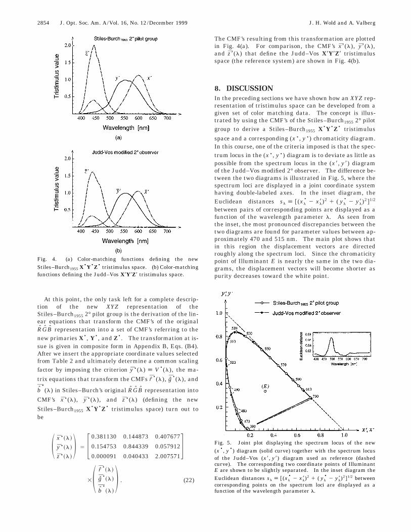
Fig. 4. (a) Color-matching functions defining the newStiles–Burch1955 X–Y–Z– tristimulus space. (b) Color-matchingfunctions defining the Judd–Vos X8Y8Z8 tristimulus space.
The CMF’s resulting from this transformation are plottedin Fig. 4(a). For comparison, the CMF’s x8(l), y8(l),and z8(l) that define the Judd–Vos X8Y8Z8 tristimulusspace (the reference system) are shown in Fig. 4(b).
8. DISCUSSIONIn the preceding sections we have shown how an XYZ rep-resentation of tristimulus space can be developed from agiven set of color matching data. The concept is illus-trated by using the CMF’s of the Stiles–Burch1955 2° pilotgroup to derive a Stiles–Burch1955 X–Y–Z– tristimulus
space and a corresponding (x–, y–) chromaticity diagram.In this course, one of the criteria imposed is that the spec-trum locus in the (x–, y–) diagram is to deviate as little aspossible from the spectrum locus in the (x8, y8) diagramof the Judd–Vos modified 2° observer. The difference be-tween the two diagrams is illustrated in Fig. 5, where thespectrum loci are displayed in a joint coordinate systemhaving double-labeled axes. In the inset diagram, theEuclidean distances sl [ @(xl
– 2 xl8)2 1 ( yl– 2 yl8)2#1/2
between pairs of corresponding points are displayed as afunction of the wavelength parameter l. As seen fromthe inset, the most pronounced discrepancies between thetwo diagrams are found for parameter values between ap-proximately 470 and 515 nm. The main plot shows thatin this region the displacement vectors are directedroughly along the spectrum loci. Since the chromaticitypoint of Illuminant E is nearly the same in the two dia-grams, the displacement vectors will become shorter aspurity decreases toward the white point.
Fig. 5. Joint plot displaying the spectrum locus of the new(x–, y–) diagram (solid curve) together with the spectrum locusof the Judd–Vos (x8, y8) diagram used as reference (dashedcurve). The corresponding two coordinate points of IlluminantE are shown to be slightly separated. In the inset diagram theEuclidean distances sl [ @(xl
– 2 xl8)2 1 ( yl– 2 yl8)2#1/2 between
corresponding points on the spectrum loci are displayed as afunction of the wavelength parameter l.
J. H. Wold and A. Valberg Vol. 16, No. 12 /December 1999 /J. Opt. Soc. Am. A 2855
The above discrepancies have their origin predomi-nantly in real differences between the color matches de-termined by the two groups of observers. This is appar-ent from a comparison of their complementarywavelengths (by necessity, reflecting characteristics ofthe observer groups and not of the representations). Asshown in Fig. 6, for the Judd–Vos modified 2° observerthe monochromatic stimuli from the long-wavelengthflank of the spectrum are complementary to monochro-matic stimuli of wavelengths up to between 493 and 494nm (by calculation 493.67 nm), whereas for theStiles–Burch1955 2° pilot group the corresponding wave-lengths are shorter and limited upward to just above 490nm (by calculation 490.36 nm).
With regard to the CMF’s derived by our method, acomment is needed on the shape of y–(l). As seen from
the graph in Fig. 4(a), y–(l) is not as smooth as the cor-responding function y8(l) of Fig. 4(b). In our procedurethere is no way of avoiding this since, on combining the Land M fundamentals of Stockman et al.30 so that the re-sult resembles the spectral luminous efficiency function,y–(l) [ V–(l) is the function obtained by adopting theirproposed weighting factors [Eqs. (10)]. Even thoughthese weighting factors may not be optimal, it neverthe-less turns out that a curve that (1) fits the CIE1988 2° spec-tral luminous efficiency function35 VM(l) [ y8(l) satis-factorily and (2) is totally free of irregularities cannot besynthesized by any linear combination of the fundamen-tal L and M response curves.
At this point we may recall Sperling’s finding that in-dividual spectral luminous efficiency functions for 2°fields, determined by flicker photometry, tend to showbends that are quite similar to those of y–(l).36 It may
therefore be that the irregularities of y–(l) [ V–(l),which at first glance may be interpreted as artifacts, ac-tually reflect characteristics of the eye’s luminous sensi-tivity that are apparent neither from the averaged spec-
Fig. 6. Complementary wavelengths of the Stiles–Burch1955 2°pilot group (solid curve) and the Judd–Vos modified 2° observer(dashed curve).
tral luminous efficiency function V(l) of the CIE1924
photometric observer19 nor from the CIE1988 2° spectralluminous efficiency function35 VM(l) of the Judd–Vosmodified 2° observer (the two functions being identical forl > 460). Taking into account the mixed origin of the1924 V(l), this may not be unlikely.
Regarding the more general aspects of our presenta-tion, purely geometrical considerations motivated the re-quirement that in the chromaticity diagram of the inter-mediate RGB representation the line connecting thechromaticity points of the X and Y primaries be tangentto the spectrum locus while having the same slope as thecorresponding line in a chosen reference diagram. An al-ternative and somewhat stricter criterion, which takesphysiological considerations into account, is to requirethat the CMF that refers to the Z primary be equal to thefundamental S response curve (S fundamental). In thechromaticity diagram of the RGB representation, the XYline is then fixed by this criterion alone. Moreover, sincethe XZ line is already determined by the luminous effi-ciency function adopted, the chromaticity point of the Xprimary—i.e., the point of intersection between the XYand the XZ line—is fixed as well. Hence what remainswill be to optimize the YZ line by using the criterion ofminimal deviation from the chosen reference diagram.
The advantage of introducing this alternative criterionis that only the X primary has no physiological correlate.(The CMF that refers to the Y primary will resemble thespectral luminous efficiency function, traceable to magno-cellular units in the visual pathway. The CMF that re-fers to the Z primary will equal the S fundamental, whichderives from S cones.) However, a condition that must befulfilled for success with such an approach is that the Sfundamental can be expressed as a linear combination ofthe CMF’s used as a database. Unfortunately, the 2°fundamental S response curve, S–(l), of Stockmanet al.30 cannot, like their proposed L and M fundamentals[L–(l) and M–(l)], be expressed as a linear combinationof the CMF’s of the Stiles–Burch1955 2° pilot group. TheS fundamental equals such a combination only in thewavelength region up to 525 nm. As a consequence ofthis lack of linear relationship, protanopic and deuteran-opic confusion points corresponding to the fundamentalsof Stockman et al.30 are not properly defined in a chroma-ticity diagram referring to the Stiles–Burch1955 2° pilotgroup. Only the tritanopic confusion point (S–) can bedetermined precisely. For wavelengths longer than 525nm, however, the values of both the S fundamental S–(l)
and the function S lin– (l) obtained by extending the range
of the linear relationship to include the entire visiblespectrum are quite small. Therefore the chromaticitypoints (L lin
– ) and (M lin– ), representing the primaries that
the L and M fundamentals of Stockman et al. would be re-ferring to if their S fundamental had been replaced byS lin– (l), can be taken as reasonable estimates of the pro-
tanopic and deuteranopic confusion points. The posi-tions of (L lin
– ) and (M lin– ) in the new (x–, y–) diagram are
determined to be (xL lin–
– , yL lin–
– ) 5 (0.737988, 0.262181) and
(xM lin–
– , yM lin–
– ) 5 (1.350806, 20.342893). The tritanopic
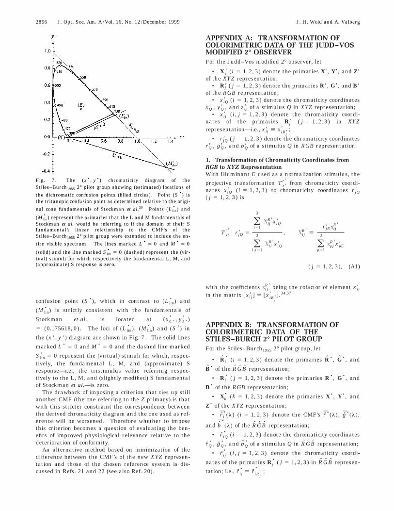
2856 J. Opt. Soc. Am. A/Vol. 16, No. 12 /December 1999 J. H. Wold and A. Valberg
confusion point (S–), which in contrast to (L lin– ) and
(M lin– ) is strictly consistent with the fundamentals of
Stockman et al., is located at (xS–– , yS–
– )
5 (0.175618, 0). The loci of (L lin– ), (M lin
– ) and (S–) in
the (x–, y–) diagram are shown in Fig. 7. The solid lines
marked L– 5 0 and M– 5 0 and the dashed line marked
S lin– 5 0 represent the (virtual) stimuli for which, respec-
tively, the fundamental L, M, and (approximate) Sresponse—i.e., the tristimulus value referring respec-tively to the L, M, and (slightly modified) S fundamentalof Stockman et al.—is zero.
The drawback of imposing a criterion that ties up stillanother CMF (the one referring to the Z primary) is thatwith this stricter constraint the correspondence betweenthe derived chromaticity diagram and the one used as ref-erence will be worsened. Therefore whether to imposethis criterion becomes a question of evaluating the ben-efits of improved physiological relevance relative to thedeterioration of conformity.
An alternative method based on minimization of thedifference between the CMF’s of the new XYZ represen-tation and those of the chosen reference system is dis-cussed in Refs. 21 and 22 (see also Ref. 20).
Fig. 7. The (x–, y–) chromaticity diagram of theStiles–Burch1955 2° pilot group showing (estimated) locations ofthe dichromatic confusion points (filled circles). Point (S–) isthe tritanopic confusion point as determined relative to the origi-nal cone fundamentals of Stockman et al.30 Points (L lin
– ) and
(M lin– ) represent the primaries that the L and M fundamentals of
Stockman et al. would be referring to if the domain of their Sfundamental’s linear relationship to the CMF’s of theStiles–Burch1955 2° pilot group were extended to include the en-tire visible spectrum. The lines marked L– 5 0 and M– 5 0
(solid) and the line marked S lin– 5 0 (dashed) represent the (vir-
tual) stimuli for which respectively the fundamental L, M, and(approximate) S response is zero.
APPENDIX A: TRANSFORMATION OFCOLORIMETRIC DATA OF THE JUDD–VOSMODIFIED 2° OBSERVERFor the Judd–Vos modified 2° observer, let
• X i8 (i 5 1, 2, 3) denote the primaries X8, Y8, and Z8of the XYZ representation;
• Rj8 ( j 5 1, 2, 3) denote the primaries R8, G8, and B8of the RGB representation;
• xiQ8 (i 5 1, 2, 3) denote the chromaticity coordinatesxQ8 , yQ8 , and zQ8 of a stimulus Q in XYZ representation;
• xij8 (i, j 5 1, 2, 3) denote the chromaticity coordi-nates of the primaries Rj8 ( j 5 1, 2, 3) in XYZrepresentation—i.e., xij8 [ xiRj8
8 ;
• rjQ8 ( j 5 1, 2, 3) denote the chromaticity coordinatesrQ8 , gQ8 , and bQ8 of a stimulus Q in RGB representation.
1. Transformation of Chromaticity Coordinates fromRGB to XYZ RepresentationWith Illuminant E used as a normalization stimulus, the
projective transformation Tx8r8 from chromaticity coordi-
nates xiQ8 (i 5 1, 2, 3) to chromaticity coordinates rjQ8( j 5 1, 2, 3) is
Tx8r8 : rjQ8 5
(i51
3
XijR8xiQ8
(l,i51
3
XilR8xiQ8
, XijR8 [
rjE8 xijR8
(r51
3
xrjR8xrE8
~ j 5 1, 2, 3 !, (A1)
with the coefficients xijR8 being the cofactor of element xij8
in the matrix @xij8 # [ @xiRj88 #.34,37
APPENDIX B: TRANSFORMATION OFCOLORIMETRIC DATA OF THESTILES–BURCH 2° PILOT GROUPFor the Stiles–Burch1955 2° pilot group, let
• Ri– (i 5 1, 2, 3) denote the primaries R–, G–, and
B– of the RGB representation;
• Rj– ( j 5 1, 2, 3) denote the primaries R–, G–, and
B– of the RGB representation;
• Xk– (k 5 1, 2, 3) denote the primaries X–, Y–, and
Z– of the XYZ representation;
• r i–(l) (i 5 1, 2, 3) denote the CMF’s r–(l), g–(l),
and b–
(l) of the RGB representation;
• r iQ– (i 5 1, 2, 3) denote the chromaticity coordinates
rQ– , gQ
– , and bQ– of a stimulus Q in RGB representation;
• r ij– (i, j 5 1, 2, 3) denote the chromaticity coordi-
nates of the primaries Rj– ( j 5 1, 2, 3) in RGB represen-
tation; i.e., r ij– [ r iR–
– ;
j
J. H. Wold and A. Valberg Vol. 16, No. 12 /December 1999 /J. Opt. Soc. Am. A 2857
1. Transformation of Chromaticity Coordinates fromRGB to RGB RepresentationWith Illuminant E used as a normalization stimulus, theprojective transformation Tr–
r– from original chromaticitycoordinates r iQ
– (i 5 1, 2, 3) to chromaticity coordinates
rjQ– ( j 5 1, 2, 3) is
Tr–r– : rjQ
– 5
(i51
3
RijR–r iQ
–
(l,i51
3
RilR–r iQ
–
, RijR– [
rjE– rij
R–
(r51
3
rrjR–rrE
–
~ j 5 1, 2, 3 !, (B1)
with rijR– being the cofactor of element r ij
– in the matrix( r ij– ) [ ( r iRj
–
– ).34,37
2. Transformation of Chromaticity Coordinates fromRGB to XYZ RepresentationWith Illuminant E used as a normalization stimulus, theprojective transformation T r–
3. Transformation of Chromaticity Coordinates fromRGB to XYZ RepresentationUsing Illuminant E as a normalization stimulus, the com-posite projective transformation T r–
x–[ T r–
x–+ T r–
r– con-
verting (directly) from chromaticity coordinates rQ– and gQ
–
to new chromaticity coordinates xQ– and yQ
– is
T r–x–
[ Tr–x–
+ Tr–r– : xkQ
– 5
(i51
3
RikX–r iQ
–
(n,i51
3
RinX–r iQ
–
,
RikX– [ (
j51
3~rjE– xkE
– !~ rijR–rjk
X–!
(r,m51
3
~ rrjR–rmk
X–!~ rrE– rmE
– !
~k 5 1, 2, 3 !,
(B3)
with r ijR– and r jk
X– defined as in Eqs. (B1) and (B2).34
4. Transformation of Color Matching Functions fromRGB to XYZ RepresentationWith Illuminant E used as a normalization stimulus, thelinear transformation T
r–x–
converting (directly) from the
original CMF’s r–(l), g–(l), and b–(l) to the new CMF’s
x–(l), y–(l), and z–(l) is
Tr–x–
: xk–~l! 5 k(
i51
3
R ikX–r i
–~l!,
RikX– [ (
j51
3~rjE– xkE
– !~ rijR–rjk
X–!
(r,m51
3
~ rrjR–rmk
X–!~ rrE– rmE
– !
,
k Þ 0 ~k 5 1, 2, 3 !, (B4)
with rijR– and rjk
X– defined as in Eqs. (B1) and (B2).34
For determining the common scaling factor k an addi-tional criterion is required, and to comply with the exist-ing CIE standard the criterion imposed is y–(l)[ x2
–(l) [ V–(l). On combination with Eq. (7), this im-plies that34
k 5cLaLi 1 cMaMi
R i2X–
, i P $1, 2, 3%. (B5)
[As indicated, Eq. (B5) is valid irrespective of the choice ofindex i.]38
ACKNOWLEDGMENTSWe thank Inger Rudvin, Thorstein Seim, Hans Vos, andDavid Brainard for valuable comments and FrancoiseVienot and Peter Walraven for their encouragement dur-ing this work.
Correspondence should be addressed to Arne Valberg,Norwegian University of Science and Technology,Department of Physics, N-7491 Trondheim, Norway.Fax, 47-7-359-1852; e-mail, [email protected].
REFERENCES AND NOTES1. F. Vienot, Report of the activity of CIE TC 1-36 ‘‘Funda-
mental chromaticity diagram with physiologically signifi-cant axes,’’ in Proceedings of the Symposium ’96 on Colour
2858 J. Opt. Soc. Am. A/Vol. 16, No. 12 /December 1999 J. H. Wold and A. Valberg
Standards for Image Technology, Vienna, 1996 (CentralBureau of the CIE, Vienna, 1996), pp. 35–40.
2. The CIE committee TC 1-36 distinguishes between the‘‘fundamental response curves,’’ representing the funda-mental spectral sensitivity functions of the three types ofcones at the corneal level, and the ‘‘cone absorption curves,’’which are derived by correcting the fundamentals by theabsorption of the lens and ocular media and the macularpigment. Hence, if Tmedia(l) denotes the spectral trans-mittance of the lens and ocular media and Tmacula(l) de-notes the spectral transmittance of the macular pigment,each cone absorption curve is given in terms of the corre-sponding fundamental response curve by the equation
cone absorption curve 5fundamental response curve
Tmedia~l!Tmacula~l!.
3. CIE, Proceedings of the 8th Session of the CIE, Cambridge,1931 (Cambridge U. Press, Cambridge, UK, 1932), pp. 19–29.
4. ISO/CIE, CIE Standard Colorimetric Observers, Publica-tion ISO/CIE 10527 (Central Bureau of the CIE, Vienna,1991).
5. W. S. Stiles and J. M. Burch, ‘‘NPL colour-matching inves-tigation: final report (1958),’’ Opt. Acta 6, 1–26 (1959).
6. R. Luther, ‘‘Aus dem Gebiet der Farbreizmetrik,’’ Z. Tech.Phys. 8, 540–558 (1927).
7. D. I. A. MacLeod and R. M. Boynton, ‘‘Chromaticity dia-gram showing cone excitation by stimuli of equal lumi-nance,’’ J. Opt. Soc. Am. 69, 1183–1186 (1979).
8. R. M. Boynton, ‘‘A system of photometry and colorimetrybased on cone excitation,’’ Color Res. Appl. 11, 244–252(1986).
9. CIE, Draft 9 of CIE TC 1-36, ‘‘Fundamental chromaticitydiagram with physiological axes’’ (Central Bureau of theCIE, Vienna, 1998).
10. W. S. Stiles and J. M. Burch, ‘‘Interim report to the Com-mission Internationale de l’Eclairage, Zurich, 1955, on theNational Physical Laboratory’s investigation of colour-matching,’’ Opt. Acta 2, 168–181 (1955).
11. J. H. Wold and A. Valberg, ‘‘Cones for colorimetry,’’ in Pro-ceedings of the 23rd Session of the CIE, New Delhi, 1995(Central Bureau of the CIE, Vienna, 1995), Vol. 1, pp. 24–27.
12. T. Smith and J. Guild, ‘‘The C.I.E. colorimetric standardsand their use,’’ Trans. Opt. Soc. 33, 73–134 (1931–1932).
13. H. S. Fairman, M. H. Brill, and H. Hemmendinger, ‘‘Howthe CIE 1931 color matching functions were derived fromWright-Guild data,’’ Color Res. Appl. 22, 11–23 (1997).
14. D. B. Judd, ‘‘Reduction of data on mixture of color stimuli,’’Bur. Stand. J. Res. 4, 515–548 (1930).
15. D. L. MacAdam, Color Measurement: Theme and Varia-tions (Springer-Verlag, Berlin, 1981).
16. The CIE RGB representation refers to Wright primaries R,G, and B, representing monochromatic stimuli of wave-lengths 700.0, 546.1, and 435.8 nm, respectively (see Refs. 3and 17). The norms of R, G, and B are defined so as toensure that the chromaticity coordinates of Illuminant Eare rE 5 gE 5 bE 5 1/3.
17. W. D. Wright, ‘‘A re-determination of the trichromatic coef-ficients of the spectral colours,’’ Trans. Opt. Soc. 30, 141–164 (1928–1929).
18. E. Schrodinger, ‘‘Uber das Verhaltnis der Vierfarben- zurDreifarbentheorie,’’ Sitzungber. Kaiserl. Wien. Akad. Wiss.Math.-Naturwiss. Kl. 134, Abt. IIa, 471–490 (1925).
19. CIE, Proceedings of the 6th Session of the CIE, Geneva, July1924 (Cambridge U. Press, Cambridge, UK, 1926), pp. 67–70.
20. Other constraints have also been considered. For in-stance, D. Brainard (topical editor, 1999, personal commu-nication) has suggested minimizing the difference betweenCMF’s (Judd–Vos versus Stiles–Burch1955) rather than be-tween the spectral loci of the chromaticity diagrams. Thisalternative seemed most attractive because of its simplicity.However, it turns out that such a minimization of differ-ences of tristimulus values in three dimensions leads to se-
vere and considerable distortions of the chromaticity dia-gram (see Refs. 21 and 22). Yet another alternative wouldbe to let the tristimulus vector to which the fundamentalS-response curve (S fundamental) refers serve as the Z pri-mary. (See Section 8 for further details.)
21. J. H. Wold and A. Valberg, ‘‘A comparison of two principlesfor deriving XYZ tristimulus spaces,’’ in The 15th Sympo-sium of the International Colour Vision Society, Gottingen,July 1999, Abstract P40.
22. J. H. Wold and A. Valberg, ‘‘The derivation of XYZ tristimu-lus spaces: a comparison of two alternative methods,’’Color Res. Appl. (to be published).
23. D. B. Judd, ‘‘CIE Technical Committee No. 7 ‘‘Colorimetryand artificial daylight,’’ Report of Secretariat United StatesCommittee,’’ in Proceedings of the 12th Session of the CIE,Stockholm, 1951 (Bureau Central de la CIE, Paris, 1951),Vol. 1, Part 7, pp. 1–60.
24. J. J. Vos, ‘‘Colorimetric and photometric properties of a 2°fundamental observer,’’ Color Res. Appl. 3, 125–128 (1978).
25. S. L. Guth, J. V. Alexander, J. I. Chumbly, C. B. Gillman,and M. M. Patterson, ‘‘Factors affecting luminance additiv-ity at threshold among normal and color-blind subjects andelaborations of a trichromatic-opponent colors theory,’’ Vi-sion Res. 8, 913–928 (1968).
26. V. C. Smith and J. Pokorny, ‘‘Spectral sensitivity of thefoveal cone photopigments between 400 and 500 nm,’’ Vi-sion Res. 15, 161–171 (1975).
27. A. Eisner and D. I. A. MacLeod, ‘‘Blue-sensitive cones donot contribute to luminance,’’ J. Opt. Soc. Am. 70, 121–123(1980).
28. W. Verdon and A. J. Adams, ‘‘Short-wavelength-sensitivecones do not contribute to mesopic luminosity,’’ J. Opt. Soc.Am. A 4, 91–95 (1987).
29. The contribution of the S cones to luminance has beensomewhat contentious. Some authors claim that S conesdo make a small contribution, whereas others maintainthat they do not. However, given that the contribution, ifany, is minor, it is convenient to assume that the S-conecontribution is zero. See, for instance, A. Stockman andL. T. Sharpe, ‘‘Cone spectral sensitivities and color match-ing,’’ in Color Vision: From Genes to Perception, K. R.Gegenfurtner and L. T. Sharpe, eds. (Cambridge U. Press,Cambridge, U.K., 1999).
30. A. Stockman, D. I. A. MacLeod, and N. E. Johnson, ‘‘Spec-tral sensitivities of the human cones,’’ J. Opt. Soc. Am. A10, 2491–2521 (1993).
31. G. Wyszecki and W. S. Stiles, Color Science: Concepts andMethods, Quantitative Data and Formulae, 2nd ed. (Wiley,New York, 1982).
32. In the paper by Stockman et al.,30 the proposed values are0.68237 and 0.35235. If we apply these values, the maxi-mum of V–(l) turns out to be 0.999777 (at 553 nm). To
normalize V–(l) to a maximum value of 1.000000, the co-efficients are multiplied by the factor 1/0.999777.
33. O. Estevez, ‘‘On the fundamental data-base of normal anddichromatic color vision,’’ Ph.D. dissertation (AmsterdamUniversity, Krips Repro Meppel, Amsterdam, 1979).
34. J. H. Wold and A. Valberg, ‘‘Mathematical description of amethod for deriving an XYZ tristimulus space,’’ Depart-ment of Physics Report Series (University of Oslo, Oslo,1999).
35. CIE, CIE 1988 2° Spectral Luminous Efficiency Function forPhotopic Vision, 1st ed., Publication CIE No. 86 (CentralBureau of the CIE, Vienna, 1990).
36. H. G. Sperling, ‘‘An experimental investigation of the rela-tionship between colour mixture and luminous efficiency,’’in Visual Problems of Colour (Her Majesty’s Stationery Of-fice, London, 1958), Vol. 1, pp. 249–247.
37. J. H. Wold, ‘‘Colorimetric transformation equations allow-ing flexible normalization,’’ Die Farbe (to be published).
38. A computer program (written in Mathematica) that deter-mines the coefficient of the transformations that convert agiven set of color matching data into a corresponding XYZrepresentation may be obtained from the authors on re-quest.