General relativistic dynamics

of binary black holes

Alexandre Le Tiec

Laboratoire Univers et TheoriesObservatoire de Paris / CNRS

Outline

1 Gravitational wave source modelling

2 Post-Newtonian approximation

3 Black hole perturbation theory

4 Effective one-body model

5 Comparisons

Outline

1 Gravitational wave source modelling

2 Post-Newtonian approximation

3 Black hole perturbation theory

4 Effective one-body model

5 Comparisons

Main sources of gravitational waves

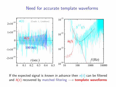
Need for accurate template waveforms

0 0.1 0.2 0.3 0.4 0.5

-2×10-19

-1×10-19

0

1×10-19

2×10-19

t (sec.)

n(t)

h(t)

10 100 1000 1000010-24

10-23

10-22

10-21

f (Hz)

h(f)

S1/2(f)

If the expected signal is known in advance then n(t) can be filteredand h(t) recovered by matched filtering −→ template waveforms

(Credit: L. Lindblom)

Need for accurate template waveforms

0 0.1 0.2 0.3 0.4 0.5

-2×10-19

-1×10-19

0

1×10-19

2×10-19

t (sec.)

n(t)

h(t)

100 h(t)

10 100 1000 1000010-24

10-23

10-22

10-21

f (Hz)

h(f)

S1/2(f)

If the expected signal is known in advance then n(t) can be filteredand h(t) recovered by matched filtering −→ template waveforms

(Credit: L. Lindblom)

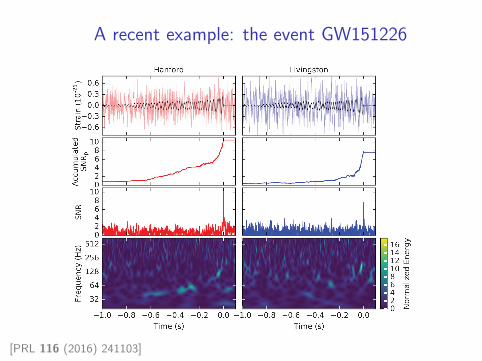
A recent example: the event GW151226

[PRL 116 (2016) 241103]

A long inspiral to merger to ringdown

[PRL 116 (2016) 241103]

Modelling coalescing compact binaries

numerical relativity

post­Newtonian theory

log10

(m2 /m

1)

0 1 2 3

0

1

2

3

4

4

log10

(r /m)

perturbation theory & self­force

(com

pact

ness

)

mass ratio

−1

Modelling coalescing compact binaries

numerical relativity

post­Newtonian theory

log10

(m2 /m

1)

0 1 2 3

0

1

2

3

4

4

log10

(r /m)

perturbation theory & self­force

(com

pact

ness

)

mass ratio

−1m

1

m2

r v2

c2∼ Gm

c2r 1

Modelling coalescing compact binaries

numerical relativity

post­Newtonian theory

log10

(m2 /m

1)

0 1 2 3

0

1

2

3

4

4

log10

(r /m)

perturbation theory & self­force

(com

pact

ness

)

mass ratio

−1 m1

m2

q ≡ m1

m2 1

Modelling coalescing compact binaries

numerical relativity

post­Newtonian theory

log10

(m2 /m

1)

0 1 2 3

0

1

2

3

4

4

log10

(r /m)

perturbation theory & self­force

(com

pact

ness

)

mass ratio

−1

m1

m2

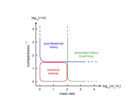
Modelling coalescing compact binaries

numerical relativity

post­Newtonian theory

log10

(m2 /m

1)

0 1 2 3

0

1

2

3

4

4

log10

(r /m)

(com

pact

ness

)

mass ratio

−1

perturbation theory & self­force

m2

M = m1 + m

2

EOB

m1

Outline

1 Gravitational wave source modelling

2 Post-Newtonian approximation

3 Black hole perturbation theory

4 Effective one-body model

5 Comparisons

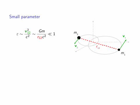
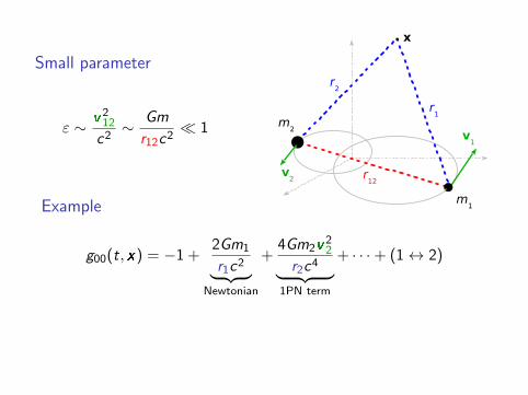
Small parameter

ε ∼ v212

c2∼ Gm

r12c2 1 m

2

m1

r12

v2

v1

Example

g00(t, x) = −1 +2Gm1

r1c2︸ ︷︷ ︸Newtonian

+4Gm2v

22

r2c4︸ ︷︷ ︸1PN term

+ · · ·+ (1↔ 2)

Notation

nPN order refers to effects O(c−2n) with respect to “Newtonian” solution

Small parameter

ε ∼ v212

c2∼ Gm

r12c2 1 m

2

m1

x

r1

r2

r12

v2

v1

Example

g00(t, x) = −1 +2Gm1

r1c2︸ ︷︷ ︸Newtonian

+4Gm2v

22

r2c4︸ ︷︷ ︸1PN term

+ · · ·+ (1↔ 2)

Notation

nPN order refers to effects O(c−2n) with respect to “Newtonian” solution

Small parameter

ε ∼ v212

c2∼ Gm

r12c2 1 m

2

m1

x

r1

r2

r12

v2

v1

Example

g00(t, x) = −1 +2Gm1

r1c2︸ ︷︷ ︸Newtonian

+4Gm2v

22

r2c4︸ ︷︷ ︸1PN term

+ · · ·+ (1↔ 2)

Notation

nPN order refers to effects O(c−2n) with respect to “Newtonian” solution

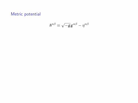
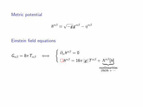
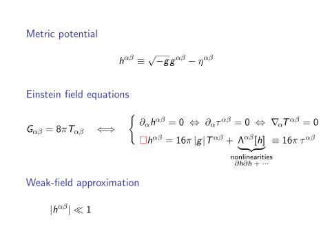
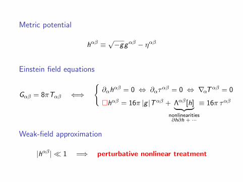
Metric potential

hαβ ≡ √−ggαβ − ηαβ

Einstein field equations

Gαβ = 8πTαβ

⇐⇒∂αh

αβ = 0

⇔ ∂αταβ = 0 ⇔ ∇αTαβ = 0

hαβ = 16π |g |Tαβ + Λαβ[h]︸ ︷︷ ︸nonlinearities∂h∂h + ···

≡ 16π ταβ

Weak-field approximation

|hαβ| 1

=⇒ perturbative nonlinear treatment

Metric potential

hαβ ≡ √−ggαβ − ηαβ

Einstein field equations

Gαβ = 8πTαβ

⇐⇒∂αh

αβ = 0

⇔ ∂αταβ = 0 ⇔ ∇αTαβ = 0

hαβ = 16π |g |Tαβ + Λαβ[h]︸ ︷︷ ︸nonlinearities∂h∂h + ···

≡ 16π ταβ

Weak-field approximation

|hαβ| 1

=⇒ perturbative nonlinear treatment

Metric potential

hαβ ≡ √−ggαβ − ηαβ

Einstein field equations

Gαβ = 8πTαβ ⇐⇒∂αh

αβ = 0

⇔ ∂αταβ = 0 ⇔ ∇αTαβ = 0

hαβ = 16π |g |Tαβ + Λαβ[h]︸ ︷︷ ︸nonlinearities∂h∂h + ···

≡ 16π ταβ

Weak-field approximation

|hαβ| 1

=⇒ perturbative nonlinear treatment

Metric potential

hαβ ≡ √−ggαβ − ηαβ

Einstein field equations

Gαβ = 8πTαβ ⇐⇒∂αh

αβ = 0

⇔ ∂αταβ = 0 ⇔ ∇αTαβ = 0

hαβ = 16π |g |Tαβ + Λαβ[h]︸ ︷︷ ︸nonlinearities∂h∂h + ···

≡ 16π ταβ

Weak-field approximation

|hαβ| 1

=⇒ perturbative nonlinear treatment

Metric potential

hαβ ≡ √−ggαβ − ηαβ

Einstein field equations

Gαβ = 8πTαβ ⇐⇒∂αh

αβ = 0 ⇔ ∂αταβ = 0

⇔ ∇αTαβ = 0

hαβ = 16π |g |Tαβ + Λαβ[h]︸ ︷︷ ︸nonlinearities∂h∂h + ···

≡ 16π ταβ

Weak-field approximation

|hαβ| 1

=⇒ perturbative nonlinear treatment

Metric potential

hαβ ≡ √−ggαβ − ηαβ

Einstein field equations

Gαβ = 8πTαβ ⇐⇒∂αh

αβ = 0 ⇔ ∂αταβ = 0 ⇔ ∇αTαβ = 0

hαβ = 16π |g |Tαβ + Λαβ[h]︸ ︷︷ ︸nonlinearities∂h∂h + ···

≡ 16π ταβ

Weak-field approximation

|hαβ| 1

=⇒ perturbative nonlinear treatment

Metric potential

hαβ ≡ √−ggαβ − ηαβ

Einstein field equations

Gαβ = 8πTαβ ⇐⇒∂αh

αβ = 0 ⇔ ∂αταβ = 0 ⇔ ∇αTαβ = 0

hαβ = 16π |g |Tαβ + Λαβ[h]︸ ︷︷ ︸nonlinearities∂h∂h + ···

≡ 16π ταβ

Weak-field approximation

|hαβ| 1

=⇒ perturbative nonlinear treatment

Metric potential

hαβ ≡ √−ggαβ − ηαβ

Einstein field equations

Gαβ = 8πTαβ ⇐⇒∂αh

αβ = 0 ⇔ ∂αταβ = 0 ⇔ ∇αTαβ = 0

hαβ = 16π |g |Tαβ + Λαβ[h]︸ ︷︷ ︸nonlinearities∂h∂h + ···

≡ 16π ταβ

Weak-field approximation

|hαβ| 1 =⇒ perturbative nonlinear treatment

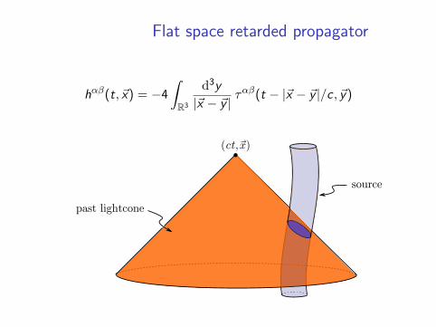
Flat space retarded propagator

hαβ(t, ~x) = −4

∫R3

d3y

|~x − ~y | ταβ(t − |~x − ~y |/c , ~y)

source

(ct,x)

past lightcone

Post-Newtonian equations of motion

m1

m2

r

v2

v1

GW

GW

n

dv1

dt= −Gm2

r2n +

A1PN

c2+A2PN

c4︸ ︷︷ ︸conservative terms

+A2.5PN

c5︸ ︷︷ ︸rad. reac.

+A3PN

c6︸ ︷︷ ︸cons. term

+A3.5PN

c7︸ ︷︷ ︸rad. reac.

+ · · ·

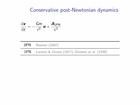
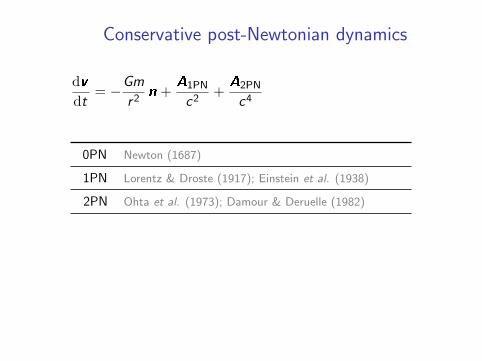
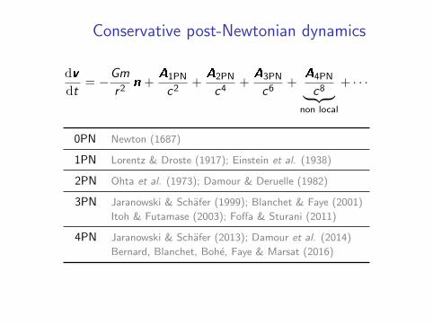
Conservative post-Newtonian dynamics

dv

dt= −Gm

r2n

+A1PN

c2+A2PN

c4+A3PN

c6+

A4PN

c8︸ ︷︷ ︸non local

+ · · ·

0PN Newton (1687)

1PN Lorentz & Droste (1917); Einstein et al. (1938)

2PN Ohta et al. (1973); Damour & Deruelle (1982)

3PN Jaranowski & Schafer (1999); Blanchet & Faye (2001)

Itoh & Futamase (2003); Foffa & Sturani (2011)

4PN Jaranowski & Schafer (2013); Damour et al. (2014)

Bernard, Blanchet, Bohe, Faye & Marsat (2016)

Poincare group symmetries −→ 10 conserved quantities

Conservative post-Newtonian dynamics

dv

dt= −Gm

r2n +

A1PN

c2

+A2PN

c4+A3PN

c6+

A4PN

c8︸ ︷︷ ︸non local

+ · · ·

0PN Newton (1687)

1PN Lorentz & Droste (1917); Einstein et al. (1938)

2PN Ohta et al. (1973); Damour & Deruelle (1982)

3PN Jaranowski & Schafer (1999); Blanchet & Faye (2001)

Itoh & Futamase (2003); Foffa & Sturani (2011)

4PN Jaranowski & Schafer (2013); Damour et al. (2014)

Bernard, Blanchet, Bohe, Faye & Marsat (2016)

Poincare group symmetries −→ 10 conserved quantities

Conservative post-Newtonian dynamics

dv

dt= −Gm

r2n +

A1PN

c2+A2PN

c4

+A3PN

c6+

A4PN

c8︸ ︷︷ ︸non local

+ · · ·

0PN Newton (1687)

1PN Lorentz & Droste (1917); Einstein et al. (1938)

2PN Ohta et al. (1973); Damour & Deruelle (1982)

3PN Jaranowski & Schafer (1999); Blanchet & Faye (2001)

Itoh & Futamase (2003); Foffa & Sturani (2011)

4PN Jaranowski & Schafer (2013); Damour et al. (2014)

Bernard, Blanchet, Bohe, Faye & Marsat (2016)

Poincare group symmetries −→ 10 conserved quantities

Conservative post-Newtonian dynamics

dv

dt= −Gm

r2n +

A1PN

c2+A2PN

c4+A3PN

c6

+A4PN

c8︸ ︷︷ ︸non local

+ · · ·

0PN Newton (1687)

1PN Lorentz & Droste (1917); Einstein et al. (1938)

2PN Ohta et al. (1973); Damour & Deruelle (1982)

3PN Jaranowski & Schafer (1999); Blanchet & Faye (2001)

Itoh & Futamase (2003); Foffa & Sturani (2011)

4PN Jaranowski & Schafer (2013); Damour et al. (2014)

Bernard, Blanchet, Bohe, Faye & Marsat (2016)

Poincare group symmetries −→ 10 conserved quantities

Conservative post-Newtonian dynamics

dv

dt= −Gm

r2n +

A1PN

c2+A2PN

c4+A3PN

c6+

A4PN

c8︸ ︷︷ ︸non local

+ · · ·

0PN Newton (1687)

1PN Lorentz & Droste (1917); Einstein et al. (1938)

2PN Ohta et al. (1973); Damour & Deruelle (1982)

3PN Jaranowski & Schafer (1999); Blanchet & Faye (2001)

Itoh & Futamase (2003); Foffa & Sturani (2011)

4PN Jaranowski & Schafer (2013); Damour et al. (2014)

Bernard, Blanchet, Bohe, Faye & Marsat (2016)

Poincare group symmetries −→ 10 conserved quantities

Conservative post-Newtonian dynamics

dv

dt= −Gm

r2n +

A1PN

c2+A2PN

c4+A3PN

c6+

A4PN

c8︸ ︷︷ ︸non local

+ · · ·

0PN Newton (1687)

1PN Lorentz & Droste (1917); Einstein et al. (1938)

2PN Ohta et al. (1973); Damour & Deruelle (1982)

3PN Jaranowski & Schafer (1999); Blanchet & Faye (2001)

Itoh & Futamase (2003); Foffa & Sturani (2011)

4PN Jaranowski & Schafer (2013); Damour et al. (2014)

Bernard, Blanchet, Bohe, Faye & Marsat (2016)

Poincare group symmetries −→ 10 conserved quantities

Gravitational-wave tails

• Gravitational waves arescattered by the bkgdcurvature generated bythe source’s mass M

space

time

space

source

• Starting at 4PN order, the near-zone metric depends onthe entire past history of the source [Blanchet & Damour 88]

δg tail00 (x, t) = −8G 2M

5c10x ix j

∫ t

−∞dt ′M

(7)ij (t ′) ln

(c(t − t ′)

2r

)

Phasing for inspiralling compact binaries

• Conservative orbital dynamics → 4PN binding energy

E (ω) = −µ2

(mω)2/3︸ ︷︷ ︸Newtonian

binding energy

(1 + · · ·

)︸ ︷︷ ︸4PN relative

correction

• Wave generation formalism → 3.5PN GW energy flux

F(ω) =32

5

µ2

m2(mω)5︸ ︷︷ ︸

Einstein’squad. formula

(1 + · · ·

)︸ ︷︷ ︸

3.5PN relativecorrection

• Energy balance → 3.5PN orbital phase and GW phase

dE

dt= −F

=⇒ dω

dt= −F(ω)

E ′(ω)=⇒ φ(t) =

∫ t

ω(t ′)dt ′

Phasing for inspiralling compact binaries

• Conservative orbital dynamics → 4PN binding energy

E (ω) = −µ2

(mω)2/3︸ ︷︷ ︸Newtonian

binding energy

(1 + · · ·

)︸ ︷︷ ︸4PN relative

correction

• Wave generation formalism → 3.5PN GW energy flux

F(ω) =32

5

µ2

m2(mω)5︸ ︷︷ ︸

Einstein’squad. formula

(1 + · · ·

)︸ ︷︷ ︸

3.5PN relativecorrection

• Energy balance → 3.5PN orbital phase and GW phase

dE

dt= −F

=⇒ dω

dt= −F(ω)

E ′(ω)=⇒ φ(t) =

∫ t

ω(t ′)dt ′

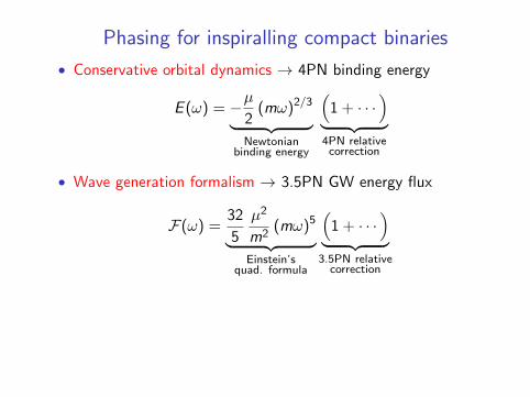
Phasing for inspiralling compact binaries

• Conservative orbital dynamics → 4PN binding energy

E (ω) = −µ2

(mω)2/3︸ ︷︷ ︸Newtonian

binding energy

(1 + · · ·

)︸ ︷︷ ︸4PN relative

correction

• Wave generation formalism → 3.5PN GW energy flux

F(ω) =32

5

µ2

m2(mω)5︸ ︷︷ ︸

Einstein’squad. formula

(1 + · · ·

)︸ ︷︷ ︸

3.5PN relativecorrection

• Energy balance → 3.5PN orbital phase and GW phase

dE

dt= −F

=⇒ dω

dt= −F(ω)

E ′(ω)=⇒ φ(t) =

∫ t

ω(t ′)dt ′

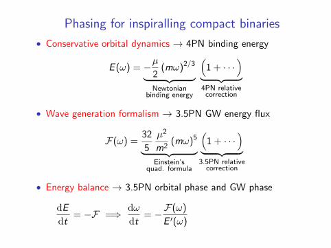
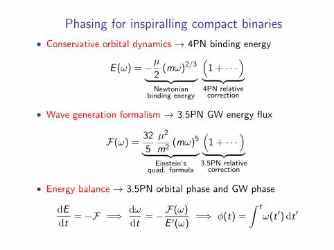
Phasing for inspiralling compact binaries

• Conservative orbital dynamics → 4PN binding energy

E (ω) = −µ2

(mω)2/3︸ ︷︷ ︸Newtonian

binding energy

(1 + · · ·

)︸ ︷︷ ︸4PN relative

correction

• Wave generation formalism → 3.5PN GW energy flux

F(ω) =32

5

µ2

m2(mω)5︸ ︷︷ ︸

Einstein’squad. formula

(1 + · · ·

)︸ ︷︷ ︸

3.5PN relativecorrection

• Energy balance → 3.5PN orbital phase and GW phase

dE

dt= −F =⇒ dω

dt= −F(ω)

E ′(ω)

=⇒ φ(t) =

∫ t

ω(t ′)dt ′

Phasing for inspiralling compact binaries

• Conservative orbital dynamics → 4PN binding energy

E (ω) = −µ2

(mω)2/3︸ ︷︷ ︸Newtonian

binding energy

(1 + · · ·

)︸ ︷︷ ︸4PN relative

correction

• Wave generation formalism → 3.5PN GW energy flux

F(ω) =32

5

µ2

m2(mω)5︸ ︷︷ ︸

Einstein’squad. formula

(1 + · · ·

)︸ ︷︷ ︸

3.5PN relativecorrection

• Energy balance → 3.5PN orbital phase and GW phase

dE

dt= −F =⇒ dω

dt= −F(ω)

E ′(ω)=⇒ φ(t) =

∫ t

ω(t ′) dt ′

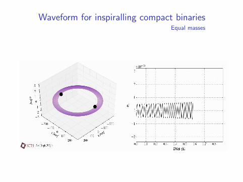
Waveform for inspiralling compact binariesEqual masses

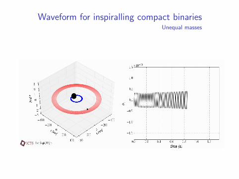
Waveform for inspiralling compact binariesUnequal masses

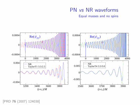
PN vs NR waveformsEqual masses and no spins

0 1000 2000 3000 4000

-0.0004

0

0.0004

NRTaylorT1 3.5/2.5

3200 3400 3600 3800

-0.004

0

0.004

(t-r*)/M

Re(ψ22 )

0 1000 2000 3000 4000

-0.0004

0

0.0004

NRTaylorT4 3.5/3.0

3500 3600 3700 3800 3900

-0.005

0

0.005

(t-r*)/M

Re(ψ22 )

[PRD 76 (2007) 124038]

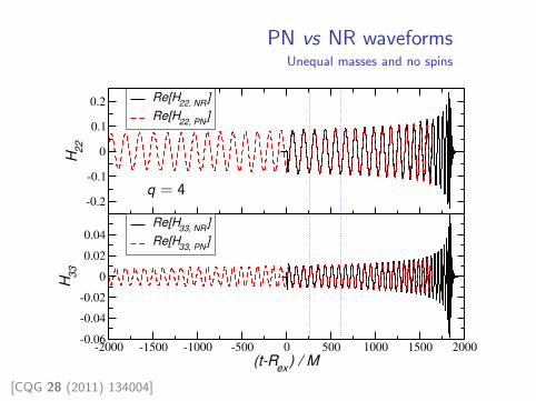
PN vs NR waveformsUnequal masses and no spins

-0.2

-0.1

0

0.1

0.2

H22

Re[H22, NR

]

Re[H22, PN

]

-2000 -1500 -1000 -500 0 500 1000 1500 2000

(t-Rex

) / M

-0.06

-0.04

-0.02

0

0.02

0.04

H33

Re[H33, NR

]

Re[H33, PN

]

q = 4

[CQG 28 (2011) 134004]

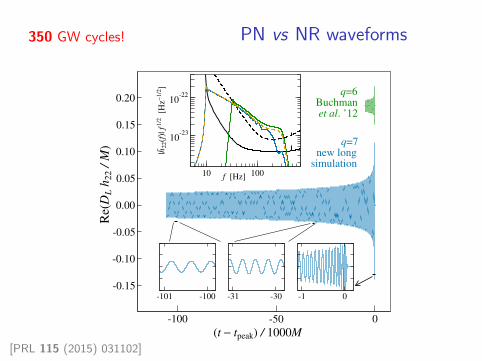
PN vs NR waveforms

-100 -50 0

-0.15

-0.10

-0.05

0.00

0.05

0.10

0.15

0.20

-1 0-31 -30-101 -100

10 100

10-23

10-22

|h~2

2(f

)| f

1/2

[H

z−1

/2]

q=6Buchmanet al. ’12

(t − tpeak) / 1000M

Re(

DL h

22

/ M

) q=7 new longsimulation

f [Hz]

350 GW cycles!

[PRL 115 (2015) 031102]

Further reading

Review articles

• Gravitational radiation from post-Newtonian sources. . .L. Blanchet, Living Rev. Rel. 17, 2 (2014)

• Post-Newtonian methods: Analytic results on the binary problemG. Schafer, in Mass and motion in general relativityEdited by L. Blanchet et al., Springer (2011)

• The post-Newtonian approximation for relativistic compact binariesT. Futamase and Y. Itoh, Living Rev. Rel. 10, 2 (2007)

Topical books

• Gravity: Newtonian, post-Newtonian, relativisticE. Poisson and C. M. Will, Cambridge University Press (2015)

• Gravitational waves: Theory and experimentsM. Maggiore, Oxford University Press (2007)

Outline

1 Gravitational wave source modelling

2 Post-Newtonian approximation

3 Black hole perturbation theory

4 Effective one-body model

5 Comparisons

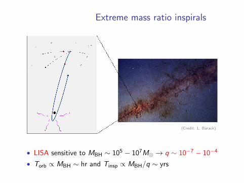
Extreme mass ratio inspirals

• LISA sensitive to MBH ∼ 105 − 107M → q ∼ 10−7 − 10−4

• Torb ∝ MBH ∼ hr and Tinsp ∝ MBH/q ∼ yrs

(Credit: L. Barack)

Large to extreme mass ratios

numerical relativity

post­Newtonian theory

log10

(m2 /m

1)

0 1 2 3

0

1

2

3

4

4

log10

(r /m)

perturbation theory & self­force

(com

pact

ness

)

mass ratio

−1 m1

m2

q ≡ m1

m2 1

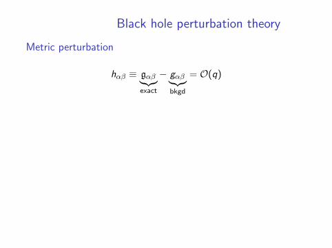
Black hole perturbation theory

Metric perturbation

hαβ ≡ gαβ︸︷︷︸exact

− gαβ︸︷︷︸bkgd

= O(q)

Lorenz gauge condition

∇αhαβ = 0

Einstein field equations

g hαβ + 2Rµ να β hµν = −16πTαβ

Linear equation but involved Green’s function

Black hole perturbation theory

Metric perturbation

hαβ ≡ gαβ︸︷︷︸exact

− gαβ︸︷︷︸bkgd

= O(q)

Lorenz gauge condition

∇αhαβ = 0

Einstein field equations

g hαβ + 2Rµ να β hµν = −16πTαβ

Linear equation but involved Green’s function

Black hole perturbation theory

Metric perturbation

hαβ ≡ gαβ︸︷︷︸exact

− gαβ︸︷︷︸bkgd

= O(q)

Lorenz gauge condition

∇αhαβ = 0

Einstein field equations

g hαβ + 2Rµ να β hµν = −16πTαβ

Linear equation but involved Green’s function

Black hole perturbation theory

Metric perturbation

hαβ ≡ gαβ︸︷︷︸exact

− gαβ︸︷︷︸bkgd

= O(q)

Lorenz gauge condition

∇αhαβ = 0

Einstein field equations

g hαβ + 2Rµ να β hµν = −16πTαβ

Linear equation but involved Green’s function

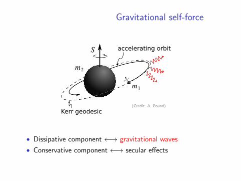
Gravitational self-force

• Dissipative component ←→ gravitational waves

• Conservative component ←→ secular effects

(Credit: A. Pound)

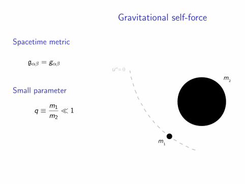
Gravitational self-force

Spacetime metric

gαβ = gαβ

+ hαβ

Small parameter

q ≡ m1

m2 1

Gravitational self-force

uα ≡ uβ∇βuα = f α[h]

m1→ 0

m2

u

Gravitational self-force

Spacetime metric

gαβ = gαβ

+ hαβ

Small parameter

q ≡ m1

m2 1

Gravitational self-force

uα ≡ uβ∇βuα = f α[h]

m1

m2

u

Gravitational self-force

Spacetime metric

gαβ = gαβ + hαβ

Small parameter

q ≡ m1

m2 1

Gravitational self-force

uα ≡ uβ∇βuα = f α[h]

m1

m2

u

h

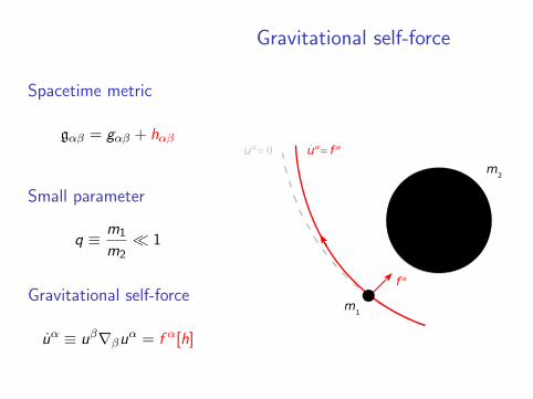
Gravitational self-force

Spacetime metric

gαβ = gαβ + hαβ

Small parameter

q ≡ m1

m2 1

Gravitational self-force

uα ≡ uβ∇βuα = f α[h]

m1

m2

f

u

Gravitational self-force

Spacetime metric

gαβ = gαβ + hαβ

Small parameter

q ≡ m1

m2 1

Gravitational self-force

uα ≡ uβ∇βuα = f α[h]

m1

m2

f

u u

f

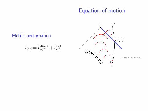
Equation of motion

Metric perturbation

hαβ = hdirectαβ + htail

αβ

MiSaTaQuWa equation

uα =(gαβ + uαuβ

)︸ ︷︷ ︸projector⊥ uα

(12∇βhtail

λσ −∇λhtailβσ

)uλuσ︸ ︷︷ ︸

“force”

≡ f α[htail]

Beware: the self-force is gauge-dependant

(Credit: A. Pound)

Equation of motion

Metric perturbation

hαβ = hdirectαβ + htail

αβ

MiSaTaQuWa equation

uα =(gαβ + uαuβ

)︸ ︷︷ ︸projector⊥ uα

(12∇βhtail

λσ −∇λhtailβσ

)uλuσ︸ ︷︷ ︸

“force”

≡ f α[htail]

Beware: the self-force is gauge-dependant

(Credit: A. Pound)

Equation of motion

Metric perturbation

hαβ = hdirectαβ + htail

αβ

MiSaTaQuWa equation

uα =(gαβ + uαuβ

)︸ ︷︷ ︸projector⊥ uα

(12∇βhtail

λσ −∇λhtailβσ

)uλuσ︸ ︷︷ ︸

“force”

≡ f α[htail]

Beware: the self-force is gauge-dependant

(Credit: A. Pound)

Equation of motion

Metric perturbation

hαβ = hdirectαβ + htail

αβ

MiSaTaQuWa equation

uα =(gαβ + uαuβ

)︸ ︷︷ ︸projector⊥ uα

(12∇βhtail

λσ −∇λhtailβσ

)uλuσ︸ ︷︷ ︸

“force”

≡ f α[htail]

Beware: the self-force is gauge-dependant

(Credit: A. Pound)

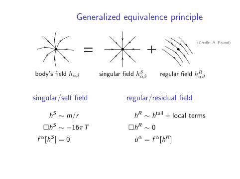
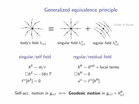
Generalized equivalence principle

singular/self field

hS ∼ m/r

hS ∼ −16πT

f α[hS ] = 0

regular/residual field

hR ∼ htail + local terms

hR ∼ 0

uα = f α[hR ]

Self-acc. motion in gαβ ⇐⇒ Geodesic motion in gαβ + hRαβ

(Credit: A. Pound)

Generalized equivalence principle

singular/self field

hS ∼ m/r

hS ∼ −16πT

f α[hS ] = 0

regular/residual field

hR ∼ htail + local terms

hR ∼ 0

uα = f α[hR ]

Self-acc. motion in gαβ ⇐⇒ Geodesic motion in gαβ + hRαβ

(Credit: A. Pound)

Generalized equivalence principle

singular/self field

hS ∼ m/r

hS ∼ −16πT

f α[hS ] = 0

regular/residual field

hR ∼ htail + local terms

hR ∼ 0

uα = f α[hR ]

Self-acc. motion in gαβ ⇐⇒ Geodesic motion in gαβ + hRαβ

(Credit: A. Pound)

Generalized equivalence principle

singular/self field

hS ∼ m/r

hS ∼ −16πT

f α[hS ] = 0

regular/residual field

hR ∼ htail + local terms

hR ∼ 0

uα = f α[hR ]

Self-acc. motion in gαβ ⇐⇒ Geodesic motion in gαβ + hRαβ

(Credit: A. Pound)

Further reading

Review articles

• Motion of small objects in curved spacetimesA. Pound, in Equations of Motion in Relativistic GravityEdited by D. Puetzfeld et al., Springer (2015)

• The motion of point particles in curved spacetimeE. Poisson, A. Pound and I. Vega, Living Rev. Rel. 14, 7 (2011)

• Gravitational self force in extreme mass-ratio inspiralsL. Barack , Class. Quant. Grav. 26, 213001 (2009)

• Analytic black hole perturbation approach to gravitational radiationM. Sasaki and H. Tagoshi, Living Rev. Rel. 6, 5 (2003)

Outline

1 Gravitational wave source modelling

2 Post-Newtonian approximation

3 Black hole perturbation theory

4 Effective one-body model

5 Comparisons

1m

2m

1m 2m

g

realE Eeff

realJ Nreal effJ effN

Real description

g eff

Effective description

Eeff(J,N) = f (Ereal(J,N))(Credit: Buonanno & Sathyaprakash 2015)

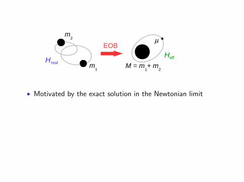
m2

M = m1+ m

2

EOB

m1

HH

real

eff

• Motivated by the exact solution in the Newtonian limit

• By construction, the EOB model:

Recovers the known PN dynamics as c−1 → 0 Recovers the geodesic dynamics when q → 0

• Idea extended to spinning binaries and to tidal effects

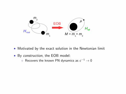
m2

M = m1+ m

2

EOB

m1

HH

real

eff

• Motivated by the exact solution in the Newtonian limit

• By construction, the EOB model:

Recovers the known PN dynamics as c−1 → 0 Recovers the geodesic dynamics when q → 0

• Idea extended to spinning binaries and to tidal effects

m2

M = m1+ m

2

EOB

m1

HH

real

eff

• Motivated by the exact solution in the Newtonian limit

• By construction, the EOB model:

Recovers the known PN dynamics as c−1 → 0

Recovers the geodesic dynamics when q → 0

• Idea extended to spinning binaries and to tidal effects

m2

M = m1+ m

2

EOB

m1

HH

real

eff

• Motivated by the exact solution in the Newtonian limit

• By construction, the EOB model:

Recovers the known PN dynamics as c−1 → 0 Recovers the geodesic dynamics when q → 0

• Idea extended to spinning binaries and to tidal effects

m2

M = m1+ m

2

EOB

m1

HH

real

eff

• Motivated by the exact solution in the Newtonian limit

• By construction, the EOB model:

Recovers the known PN dynamics as c−1 → 0 Recovers the geodesic dynamics when q → 0

• Idea extended to spinning binaries and to tidal effects

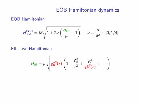
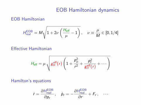
EOB Hamiltonian dynamics

EOB Hamiltonian

HEOBreal = M

√1 + 2ν

(Heff

µ− 1

), ν ≡ µ

M∈ [0, 1/4]

Effective Hamiltonian

Heff = µ

√√√√g efftt (r)

(1 +

p2φ

r2+

p2r

g effrr (r)

+ · · ·)

Hamilton’s equations

r =∂HEOB

real

∂pr, pr = −∂H

EOBreal

∂r+ Fr , · · ·

EOB Hamiltonian dynamics

EOB Hamiltonian

HEOBreal = M

√1 + 2ν

(Heff

µ− 1

), ν ≡ µ

M∈ [0, 1/4]

Effective Hamiltonian

Heff = µ

√√√√g efftt (r)

(1 +

p2φ

r2+

p2r

g effrr (r)

+ · · ·)

Hamilton’s equations

r =∂HEOB

real

∂pr, pr = −∂H

EOBreal

∂r+ Fr , · · ·

EOB Hamiltonian dynamics

EOB Hamiltonian

HEOBreal = M

√1 + 2ν

(Heff

µ− 1

), ν ≡ µ

M∈ [0, 1/4]

Effective Hamiltonian

Heff = µ

√√√√g efftt (r)

(1 +

p2φ

r2+

p2r

g effrr (r)

+ · · ·)

Hamilton’s equations

r =∂HEOB

real

∂pr, pr = −∂H

EOBreal

∂r+ Fr , · · ·

EOB effective metric

Effective metric

ds2eff = −g eff

tt (r ; ν)dt2 + g effrr (r ; ν)dr2 + r2 dΩ2

Effective potentials

g efftt = 1− 2M

r︸ ︷︷ ︸Schwarzschild

+ ν

[2

(M

r

)3

+

(94

3− 41

32π2

)(M

r

)4

+ · · ·]

︸ ︷︷ ︸finite mass-ratio “deformation”

Pade resummation

Motivation: improve convergence of PN series in strong-field regime

EOB effective metric

Effective metric

ds2eff = −g eff

tt (r ; ν)dt2 + g effrr (r ; ν)dr2 + r2 dΩ2

Effective potentials

g efftt = 1− 2M

r︸ ︷︷ ︸Schwarzschild

+ ν

[2

(M

r

)3

+

(94

3− 41

32π2

)(M

r

)4

+ · · ·]

︸ ︷︷ ︸finite mass-ratio “deformation”

Pade resummation

Motivation: improve convergence of PN series in strong-field regime

EOB effective metric

Effective metric

ds2eff = −g eff

tt (r ; ν)dt2 + g effrr (r ; ν)dr2 + r2 dΩ2

Effective potentials

g efftt = 1− 2M

r︸ ︷︷ ︸Schwarzschild

+ ν

[2

(M

r

)3

+

(94

3− 41

32π2

)(M

r

)4

+ · · ·]

︸ ︷︷ ︸finite mass-ratio “deformation”

Pade resummation

Motivation: improve convergence of PN series in strong-field regime

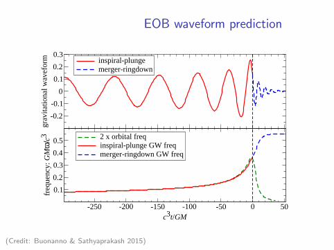
EOB waveform prediction

-0.2-0.1

00.10.20.3

grav

itatio

nal w

avef

orm inspiral-plunge

merger-ringdown

-250 -200 -150 -100 -50 0 50c3t/GM

0.10.20.30.40.5

freq

uenc

y: G

Mω

/c3 2 x orbital freq

inspiral-plunge GW freqmerger-ringdown GW freq

(Credit: Buonanno & Sathyaprakash 2015)

EOB vs NR waveformsEqual masses and no spins

[PRD 79 (2009) 081503]

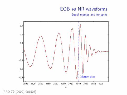
EOB vs NR waveformsEqual masses and no spins

3800 3820 3840 3860 3880 3900 3920 3940 3960 3980 4000

−0.3

−0.2

−0.1

0

0.1

0.2

0.3

t

Merger time

[PRD 79 (2009) 081503]

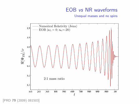
EOB vs NR waveformsUnequal masses and no spins

[PRD 79 (2009) 081503]

EOB vs NR waveformsEqual masses and aligned spins

0 1000 2000 3000 4000 5000 6000(t − r

*) / M

-0.4

-0.2

0.0

0.2

0.4R

e(R

/M h

22)

6000 6100 6200 6300 6400 6500(t − r

*) / M

-0.4

-0.2

0.0

0.2

0.4

Re(

R/M

h22

)NREOB

(q, χ1, χ

2) = (1, +0.98, +0.98)

[PRD 89 (2014) 061502]

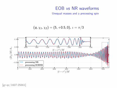
EOB vs NR waveformsUnequal masses and a precessing spin

(q, χ1, χ2) = (5,+0.5, 0), ι = π/3

0 1000 2000 3000 4000 5000 6000 7000

(t− r∗)/M

−0.05

0.00

0.05

0.10

(DL/M

)h

+

precessing NRprecessing EOBNR

6900 7000 7100 7200 7300 7400 7500

(t− r∗)/M

[gr-qc/1607.05661]

Recent developments

• Extension of EOB model to spinning binaries[Barausse & Buonanno (2011), Nagar (2011), Damour & Nagar (2014)]

• Addition of tidal interactions for neutrons stars[Damour & Nagar (2010), Bini et al. (2012), Hinderer et al. (2016)]

• Various calibrations to numerical relativity simulations[Damour & Nagar (2014), Pan et al. (2014), Taracchini et al. (2014)]

• Calibration of EOB potentials by comparison to self-force[Barack et al. (2011), Le Tiec (2015), Akcay & van de Meent (2016)]

Recent developments

• Extension of EOB model to spinning binaries[Barausse & Buonanno (2011), Nagar (2011), Damour & Nagar (2014)]

• Addition of tidal interactions for neutrons stars[Damour & Nagar (2010), Bini et al. (2012), Hinderer et al. (2016)]

• Various calibrations to numerical relativity simulations[Damour & Nagar (2014), Pan et al. (2014), Taracchini et al. (2014)]

• Calibration of EOB potentials by comparison to self-force[Barack et al. (2011), Le Tiec (2015), Akcay & van de Meent (2016)]

Recent developments

• Extension of EOB model to spinning binaries[Barausse & Buonanno (2011), Nagar (2011), Damour & Nagar (2014)]

• Addition of tidal interactions for neutrons stars[Damour & Nagar (2010), Bini et al. (2012), Hinderer et al. (2016)]

• Various calibrations to numerical relativity simulations[Damour & Nagar (2014), Pan et al. (2014), Taracchini et al. (2014)]

• Calibration of EOB potentials by comparison to self-force[Barack et al. (2011), Le Tiec (2015), Akcay & van de Meent (2016)]

Recent developments

• Extension of EOB model to spinning binaries[Barausse & Buonanno (2011), Nagar (2011), Damour & Nagar (2014)]

• Addition of tidal interactions for neutrons stars[Damour & Nagar (2010), Bini et al. (2012), Hinderer et al. (2016)]

• Various calibrations to numerical relativity simulations[Damour & Nagar (2014), Pan et al. (2014), Taracchini et al. (2014)]

• Calibration of EOB potentials by comparison to self-force[Barack et al. (2011), Le Tiec (2015), Akcay & van de Meent (2016)]

Further reading

Review articles

• Sources of gravitational waves: Theory and observationsA. Buonanno and B. S. Sathyaprakash, in General relativity andgravitation: A centennial perspectiveEdited by A. Ashtekar et al., Cambridge University Press (2015)

• The general relativistic two body problem and the EOB formalismT. Damour, in General relativity, cosmology and astrophysicsEdited by J. Bicak and T. Ledvinka, Springer (2014)

• The effective one-body description of the two-body problemT. Damour and A. Nagar, in Mass and motion in general relativityEdited by L. Blanchet et al., Springer (2011)

Outline

1 Gravitational wave source modelling

2 Post-Newtonian approximation

3 Black hole perturbation theory

4 Effective one-body model

5 Comparisons

numerical relativity

post­Newtonian theory

log10

(m2 /m

1)

0 1 2 3

0

1

2

3

4

4

log10

(r /m)

perturbation theory & self­force

(com

pact

ness

)

mass ratio

−1

numerical relativity

post­Newtonian theory

log10

(m2 /m

1)

0 1 2 3

0

1

2

3

4

4

log10

(r /m)

perturbation theory & self­force

(com

pact

ness

)

mass ratio

−1 ?

??

Why?

• Independent checks of long and complicated calculations

• Identify domains of validity of approximation schemes

• Extract information inaccessible to other methods

• Develop a universal model for compact binaries

How?

8 Use the same coordinate system in all calculations

4 Using coordinate-invariant relationships

What?

• Gravitational waveforms at future null infinity

• Conservative effects on the orbital dynamics

Why?

• Independent checks of long and complicated calculations

• Identify domains of validity of approximation schemes

• Extract information inaccessible to other methods

• Develop a universal model for compact binaries

How?

8 Use the same coordinate system in all calculations

4 Using coordinate-invariant relationships

What?

• Gravitational waveforms at future null infinity

• Conservative effects on the orbital dynamics

Why?

• Independent checks of long and complicated calculations

• Identify domains of validity of approximation schemes

• Extract information inaccessible to other methods

• Develop a universal model for compact binaries

How?

8 Use the same coordinate system in all calculations

4 Using coordinate-invariant relationships

What?

• Gravitational waveforms at future null infinity

• Conservative effects on the orbital dynamics

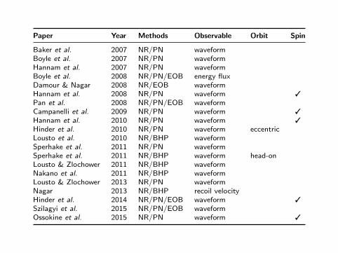
Paper Year Methods Observable Orbit Spin

Baker et al. 2007 NR/PN waveformBoyle et al. 2007 NR/PN waveformHannam et al. 2007 NR/PN waveformBoyle et al. 2008 NR/PN/EOB energy fluxDamour & Nagar 2008 NR/EOB waveformHannam et al. 2008 NR/PN waveform 3Pan et al. 2008 NR/PN/EOB waveformCampanelli et al. 2009 NR/PN waveform 3Hannam et al. 2010 NR/PN waveform 3Hinder et al. 2010 NR/PN waveform eccentricLousto et al. 2010 NR/BHP waveformSperhake et al. 2011 NR/PN waveformSperhake et al. 2011 NR/BHP waveform head-onLousto & Zlochower 2011 NR/BHP waveformNakano et al. 2011 NR/BHP waveformLousto & Zlochower 2013 NR/PN waveformNagar 2013 NR/BHP recoil velocityHinder et al. 2014 NR/PN/EOB waveform 3Szilagyi et al. 2015 NR/PN/EOB waveformOssokine et al. 2015 NR/PN waveform 3

Paper Year Methods Observable Orbit Spin

Detweiler 2008 BHP/PN redshift observableBlanchet et al. 2010 BHP/PN redshift observableDamour 2010 BHP/EOB ISCO frequencyMroue et al. 2010 NR/PN periastron advanceBarack et al. 2010 BHP/EOB periastron advanceFavata 2011 BHP/PN/EOB ISCO frequencyLe Tiec et al. 2011 NR/BHP/PN/EOB periastron advanceDamour et al. 2012 NR/EOB binding energyLe Tiec et al. 2012 NR/BHP/PN/EOB binding energyAkcay et al. 2012 BHP/EOB redshift observableHinderer et al. 2013 NR/EOB periastron advance 3Le Tiec et al. 2013 NR/BHP/PN periastron advance 3Bini & DamourShah et al.Blanchet et al.

2014 BHP/PN redshift observable

Dolan et al.Bini & Damour

2014 BHP/PN precession angle 3

Isoyama et al. 2014 BHP/PN/EOB ISCO frequency 3Akcay et al. 2015 BHP/PN averaged redshift eccentricShah & Pound 2015 BHP/PN precession angle 3Zimmerman et al. 2016 NR/PN surface gravityAkcay et al. 2016 BHP/PN precession angle eccentric

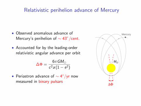
Relativistic perihelion advance of Mercury

• Observed anomalous advance ofMercury’s perihelion of ∼ 43”/cent.

• Accounted for by the leading-orderrelativistic angular advance per orbit

∆Φ =6πGM

c2a (1− e2)

• Periastron advance of ∼ 4/yr nowmeasured in binary pulsars

M⊙

Mercury

Periastron advance in black hole binaries

• Generic eccentric orbit parametrized bythe two invariant frequencies

Ωr =2π

P, Ωϕ =

1

P

∫ P

0ϕ(t) dt

• Periastron advance per radial period

K ≡ Ωϕ

Ωr= 1 +

∆Φ

2π

• In the circular orbit limit e → 0, therelation K (Ωϕ) is coordinate-invariant

m2

m1

t=0 t=P

Periastron advance vs orbital frequency

1.2

1.3

1.4

1.5

SchwEOBGSFνPNGSFq

0.01 0.02 0.03

-0.01

0

0.01

mΩϕ

KδK/K

1:1

[PRL 107 (2011) 141101]

Periastron advance vs orbital frequency

1.2

1.3

1.4

1.5

SchwEOBGSFνPNGSFq

0.01 0.02 0.03

-0.01

0

0.01

mΩϕ

KδK/K

q = m1/m2

= m1m2 /m2ν1:1

[PRL 107 (2011) 141101]

Periastron advance vs mass ratio

0 0.2 0.4 0.6 0.8 1

-0.024

-0.018

-0.012

-0.006

0

EOB

GSFνPN

0 0.5 1

-0.08

-0.04

0

0.04

Schw

GSFq

q

δK

/K

[PRL 107 (2011) 141101]