General relativity - Accueilo.castera.free.fr/zip/General_relativity.pdfGeneral relativity is a...

General relativityDr. Luigi E. Masciovecchio

[email protected]

first published on http://mio.discoremoto.alice.it/luigimasciovecchio/, October 2011

available as notebook and PDF on http://sites.google.com/site/luigimasciovecchio/

Print@"Revision ", IntegerPart@Date@DDDRevision 82013, 7, 30, 8, 0, 59<

A) INTRODUCTION

Dear Colleagues,

This is my personal Mathematica notebook on Albert Einstein's genial general theory of relativity. This document

wasn't originally intended for publication, but a few formulas and tricks are maybe of interest to you, so here they are. The

code seems to work well and I added some comments to make it more understandable. This is not an introduction to this

field, so use it at your own risk!

The main point about this work is to show how to do the typical mathematics of general relativity easily and rigor-

ously with Mathematica. In addition, I "streamlined" a little bit the derivation of some classical results (perihelion advance,

bending of light etc.).

As main textbook I have chosen the excellent and brilliantly instructive "A short course in general relativity" by

James Foster and J.David Nightingale. Mathematica together with the packages Tensorial and GeneralRelativity have been

used by David Park to do all the derivations, examples and exercises of this textbook. Most of the present notebook is

actually a rewrite of Park's very fine original work.

Once again, the combination of a good textbook and Mathematica provides a fun, easy and mathematical rigorous

learning environment that stimulates greatly understanding and own experiments with the formulas. Don't miss it!

* * *

General relativity is a metric theory of gravitation. At its core are Einstein's field equations, which describe the relation between

the geometry of a four-dimensional, pseudo-Riemannian manifold representing spacetime, and the energy-momentum contained

in that spacetime. First published by Albert Einstein in 1915 as a tensor equation, the Einstein's field equations equate spacetime

curvature (expressed by the Einstein tensor) with the energy and momentum within that spacetime (expressed by the energy-

momentum-stress tensor). General relativity's predictions have been confirmed in all observations and experiments to date.

Although general relativity is not the only relativistic theory of gravity, it is the simplest theory that is consistent with experimen-

tal data. (Wikipedia, 2011)

General relativity is a geometric theory and incorporates special relativity in the sense that locally the spacetime of the general

theory is like that of the special theory. So it's important for the sake of conceptual cleanness to derive in your course first special

relativity from the basic geometrical spacetime symmetries without using the postulate of constant speed of light or any other

"unneeded physics" (see for example Jean-Marc Lévy-Leblond, "One more derivation of the Lorentz transformation", American

Journal of Physics 44, 271-277 (1976); visit http://o.castera.free.fr for more information).

Valuable web resources on general relativity:• David Park, Mathematica notebooks (2005) based on "A short course in general relativity" (Foster/Nightingale)

• See books.google.com or the Springer editor web site for a preview of the above-mentioned textbook.

• Florian Schrack "Gravitation - Theorien, Effekte und Simulation am Computer" (2002)

• Gerard ’t Hooft "Introduction to General Relativity" (2007)

• Matt Visser "Math 464: Notes on Differential Geometry" (2009)

• Matt Visser "Math 465: Notes on General Relativity and Cosmology" (2009)

• Norbert Dragon "Geometrie der Relativitätstheorie" (2011)

• Sean Carroll "Lecture Notes on General Relativity" (1997)

• Tom Marsh "Notes for PX436, General Relativity" (2009)

• Clifford M. Will "The Confrontation between General Relativity and Experiment", Living Rev. Relativity, 9, (2006)

• Neil Ashby "Relativity in the Global Positioning System", Living Rev. Relativity, 6, (2003)

• Wikipedia: "General relativity", "Allgemeine Relativitätstheorie" and links

• General relativity video courses (Charles Bailyn, Alexander Maloney, Lenny Susskind)

General_relativity.nb 1

Valuable web resources on general relativity:• David Park, Mathematica notebooks (2005) based on "A short course in general relativity" (Foster/Nightingale)

• See books.google.com or the Springer editor web site for a preview of the above-mentioned textbook.

• Florian Schrack "Gravitation - Theorien, Effekte und Simulation am Computer" (2002)

• Gerard ’t Hooft "Introduction to General Relativity" (2007)

• Matt Visser "Math 464: Notes on Differential Geometry" (2009)

• Matt Visser "Math 465: Notes on General Relativity and Cosmology" (2009)

• Norbert Dragon "Geometrie der Relativitätstheorie" (2011)

• Sean Carroll "Lecture Notes on General Relativity" (1997)

• Tom Marsh "Notes for PX436, General Relativity" (2009)

• Clifford M. Will "The Confrontation between General Relativity and Experiment", Living Rev. Relativity, 9, (2006)

• Neil Ashby "Relativity in the Global Positioning System", Living Rev. Relativity, 6, (2003)

• Wikipedia: "General relativity", "Allgemeine Relativitätstheorie" and links

• General relativity video courses (Charles Bailyn, Alexander Maloney, Lenny Susskind)

Note:è Mathematica by Wolfram Research is a (fabulous) computer algebra system.

è A notebook is an interactive Mathematica document (extension .nb).

è Tensorial 3.0 (R. Cabrera, D. Park, J.-F. Gouyet, August 2005) is a general-purpose tensor calculus package for Mathematica

Version 4.1 or later.

è TGeneralRelativity1`GeneralRelativity` (D. Park, 29 January 2005) is a subpackage for the Tensorial package that adds

routines useful in special and general relativity. (This also automatically loads the regular Tensorial package.)

Print@"This system is:"D8"ProductIDName", "ProductVersion"< . $ProductInformation

ReadList@"!ver", StringD@@2DD8$MachineType, $ProcessorType, $ByteOrdering, $SystemCharacterEncoding<This system is:

8Mathematica, 5.2 for Microsoft Windows HJune 20, 2005L<Windows 98 @versione 4.10.1998D8PC, x86, -1, WindowsANSI<

B) HELP

(Extracted from the Tensorial package help.)

x,∆,g,G are the standard set of tensor labels used in all Tensorial derivative routines. They tell the routines which labels

will be considered to represent the coordinates x, Kronecker ∆, metric tensor g and Christoffel symbol G.

DeclareBaseIndices[index..] declares the base indices for the underlying linear space.

DeclareIndexFlavor[flavorname,flavorform...] will add the index flavors to the IndexFlavors list and establish

the Format for displaying indices with the given flavor name.

ToArrayValues[baseindices][expr] will convert the expression to a vector, matrix or array by expansion and substitu-

tion of any stored values.

EvaluateDotProducts[e,g,metricsimplify:True][expr] expands Dot products of vectors expressed in a given basis

e using the metric tensor g. Metric simplification is performed if the default argument metricsimplify is True.

LinearBreakout[f1,f2,...][v1,v2,...][expr] will break out the linear terms of any expressions within expr that

have heads matching the patterns fi over variables matching the patterns vj.

SetMetricValues[g,metricmatrix,flavor:Identity] creates value definitions for the up and down forms of the

metric tensor using the label g and a metric matrix.

CoordinateToTensors[r,Θ,Φ...,coord:x,flavor:Identity][expr] will convert the coordinate symbols in the

expression to the corresponding indexed tensors. The optional arguments coord and flavor give the coordinate label and index

flavor to use. Their default values are x and plain.General_relativity.nb 2

CoordinateToTensors[r,Θ,Φ...,coord:x,flavor:Identity][expr] will convert the coordinate symbols in the

expression to the corresponding indexed tensors. The optional arguments coord and flavor give the coordinate label and index

flavor to use. Their default values are x and plain.

SetChristoffelValueRules[xu[i,metricmatrix,G,simplification:Identity] calculates and stores substitution

rules for the Christoffel values of Gudd[i,j,k] and Gddd[i,j,k] from the values of metricmatrix and the xu[i] vector pattern.

SelectedTensorRules[label,pattern] will select the rules for label whose right hand sides are nonzero and whose left

hand sides match the pattern.

SimplifyTensorSum[expr] will check that all terms in a tensor sum have valid indices,that the free indices are the same in

all terms,and will simplify the sum by matching dummy indices in all terms that have the same index structure.

ExpandCovariantD[x,∆,g,G,a][expr] will expand first order covariant derivatives of tensors using x as the label for

the coordinates, ∆ as the label for the Kronecker, g as the label for the metric tensor and G as the label for Christoffel symbols.

The introduced dummy index will be a.

MapLevelParts[function,topposition,levelpositions][expr] will map the function onto the selected level

positions in an expression. The function is applied to them as a group and they are replaced with a single new expression. Other

parts not specified on the list are left unchanged.

C) PHYSICAL CONSTANTS

Some physical constants as given by Mathematica.

Print@"Miscellaneous`PhysicalConstants`:"D<< Miscellaneous`PhysicalConstants`

<< MiscellaneousÙnits`8SpeedOfLight, GravitationalConstant, CosmicBackgroundTemperature, HubbleConstant<9HubbleConstant-1, AgeOfUniverse HubbleConstant-1, Convert@AgeOfUniverse, YearD=9"Earth:", EarthMass, EarthRadius, "Sun:",

ConvertASolarSchwarzschildRadius SpeedOfLight2 H2 GravitationalConstantL, KilogramE,SolarRadius, SolarSchwarzschildRadius=

Miscellaneous`PhysicalConstants`:

:299792458 MeterSecond

,6.673 ´ 10-11 Meter2 Newton

Kilogram2, 2.726 Kelvin,

3.2 ´ 10-18

Second>

93.125 ´ 1017 Second, 1.504, 1.49036 ´ 1010 Year=9Earth:, 5.9742 ´ 1024 Kilogram, 6 378 140 Meter,

Sun:, 1.9888 ´ 1030 Kilogram, 6.9599 ´ 108 Meter, 2953.25 Meter=PrintA"Gravitational constant\nG = ",

ConvertAGravitationalConstant, Kilogram-1 Meter3 Second-2E, " = ",

ConvertAGravitationalConstant, Gram-1 Centimeter3 Second-2EEConvertA8 Π GravitationalConstant SpeedOfLight2, Meter KilogramE;PrintA"Einsteinsche Gravitationskonstante in SexlUrbantke S.69\nΚ = 8 Π G c-2 = ", %, " = ",

ConvertA%, Gram-1 Centimeter EEPrintA"coupling constant in FosterNightingale p.113\nΚ = - 8 Π G c-4 = ",

- %% SpeedOfLight2E


Gravitational constant

G =6.673´10-11 Meter3

Kilogram Second2=

6.673´10-8 Centimeter3

Gram Second2

Einsteinsche Gravitationskonstante in SexlUrbantke S.69

Κ = 8 Π G c-2 =1.86603´10-26 Meter

Kilogram=

1.86603´10-27 Centimeter

Gram

coupling constant in FosterNightingale p.113

Κ = - 8 Π G c-4 = -2.07624´10-43 Second2

Kilogram Meter

I will use the CODATA 2010 values. (See http://physics.nist.gov/ for updates.)

PrintA"CODATA 2010: G = 6.673 84H80L´10-11 m3 kg-1 s-2"EPrintA"Κ = - 8 Π G c-4 = ",

NumberFormA-8 Π 6.67384 ´ 10-11 I299 792 4584M, 7 E, " m-1 kg-1 s2"ECODATA 2010: G = 6.673 84H80L´10-11 m3 kg-1 s-2

Κ = - 8 Π G c-4 = -2.076504´10-43 m-1 kg-1 s2

D) OWN (?) CONSIDERATIONS

Special relativity teaches us how spacetime dictates the behavior of matter-energy and general relativity teaches us how matter-

energy influences the behavior of spacetime. We could say that this two entities, spacetime and matter-energy, are in some kind

of interaction. Starting from a heuristic principle that states that entities who can interact can not be completely different "in

essence", we could tentatively postulate a symmetry between spacetime and matter-energy, implying the possibility of a transfor-

mation of spacetime into matter-energy and vice-versa. So it's maybe sensible to ask:

• How much spacetime can we get from a given quantity of matter-energy or vice-versa? What is the conversion factor Λ between

(geometrized) spacetime and matter-energy (1 m4 =` Λ · 1 J)? Is Λ a universal constant?

• What are the observable signatures of spacetime V matter-energy transformations?

• How "expands" newly created spacetime in some finite region into the rest of the Universe? How works the local "collapse" of

the universe caused by the destruction of a finite piece of spacetime?

• How works the spacetime - matter-energy - transformation at a fundamental level?

Since wild speculations don't cost a thing, we can go further and postulate the existence of a substance called "Essenz" in which

matter-energy and spacetime are not separated entities and which constitutes all of the Universe at some point. We can assume

that the Big Bang represents the moment of the evolution of the Universe where the Essenz undergoes a phase transition separat-

ing into the two components spacetime and matter-energy. Since then we have "matter-energy acting on the stage of spacetime"

and we can define (at most locally) a metric to measure space and time. We said that the Essenz undergoes a phase transition at

some point: this means that this substance is not static. But the time coordinate that we need to catalogue events in the pre-Big-

Bang era has to be interpreted as an intrinsic parameter of the Essenz. This intrinsic time parameter must not necessarily be a

measurable quantity (if there is no metric) but may defines only an order relation between events, the evolution of the Essenz

proceeding by "leaps" much like today quantum systems evolves (e.g. successive decays in a radioactive series). Perhaps this

analogy is not accidental and points to some connection between quantum mechanics and spacetime physics!

Well, as I said, wild speculations don't cost a thing...


E) CALCULATIONS FROM

James Foster, J.David NightingaleA SHORT COURSE IN GENERAL RELATIVITY

(3.ed., 2006)

with Mathematica code by David Park (2005, for the 2. ed. [1995])partially modified, corrected and simplified by Luigi E. Masciovecchio (2011)

Utilization note: Every of the following Mathematica subsections should be evaluated by its own! The initialization code for a

subsection ends with a horizontal line. I present here only my limited set of calculations from the textbook, for a complete (!) and

extensively commented set see the huge work by David Park.

Chapter 1: Vector and tensor fields

1.0 Introduction p. 7

FN: "Our starting point is a consideration of vector fields in the familiar setting of three-dimensional Euclidean space and how

they can be handled using arbitrary curvilinear coordinate systems. We then go on to extend and generalize these ideas in two

different ways, first by admitting tensor fields, and second by allowing the dimension of the space to be arbitrary and its geome-

try to be non-Euclidean."

1.1 Coordinate systems in Euclidean space p. 7 - 13 (nonsuffix notation)

Keywords: Cartesian and non-Cartesian coordinate systems, coordinate surfaces and curves, position vector of points in space,

natural and dual basis in 3D Euclidean space.

Mathematica resources on coordinate systems (see the standard add-on package Calculus`VectorAnalysis`)

<< Calculus`VectorAnalysis`

CoordinatesToCartesian@Coordinates@SphericalD, SphericalD8Coordinates@SphericalD, CoordinateRanges@SphericalD<CoordinatesToCartesian@8u, v, w<, SphericalDCoordinatesFromCartesian@8x, y, z<, SphericalD8Rr Cos@PphiD Sin@TthetaD, Rr Sin@PphiD Sin@TthetaD, Rr Cos@TthetaD<88Rr, Ttheta, Pphi<, 80 £ Rr < ¥, 0 £ Ttheta £ Π, -Π < Pphi £ Π<<8u Cos@wD Sin@vD, u Sin@vD Sin@wD, u Cos@vD<: x2 + y2 + z2 , ArcCosB z

x2 + y2 + z2F, ArcTan@x, yD>


CoordinatesToCartesian@8u, v, w<, ParaboloidalD:u v Cos@wD, u v Sin@wD, 1

2Iu2 - v2M>

CoordinatesToCartesian@8u, v, w<, ParabolicCylindricalD:12

Iu2 - v2M, u v, w>

Example 1.1.2, p.10. "spherical coordinates - natural basis/dual basis"

x@u_, v_, w_D := u Cos@wD Sin@vD;y@u_, v_, w_D := u Sin@vD Sin@wD;z@u_, v_, w_D := u Cos@vD;r = 8x@u, v, wD, y@u, v, wD, z@u, v, wD<;H* inverted equations *Luu@x_, y_, z_D := x2 + y2 + z2 ;

vv@x_, y_, z_D := ArcCosBz x2 + y2 + z2 F;ww@x_, y_, z_D := ArcTan@x, yD;$Assumptions = 80 £ u < ¥, 0 £ v £ Π, -Π < w £ Π, 8x, y, z< Î Reals<;gradxyz@scalarfield_D := 9¶xscalarfield, ¶yscalarfield, ¶zscalarfield=Print@"Position and natural basis 8eu,ev,ew< in spherical coordinates u,v,w"Dr MatrixForm

naturalbasisuvw = 8¶ur, ¶vr, ¶wr<;MatrixForm naturalbasisuvwHnaturalbasisuvw.Transpose@naturalbasisuvwDL Simplify MatrixForm

PrintA"8eu,ev,ew< in u,v,w"Enormnaturalbasisuvw = naturalbasisuvw HSimplify@Sqrt@Abs@ð.ð DDD & naturalbasisuvwL;MatrixForm normnaturalbasisuvwnormnaturalbasisuvw.Transpose@normnaturalbasisuvwD Simplify MatrixForm

Position and natural basis 8eu,ev,ew< in spherical coordinates u,v,w

u Cos@wD Sin@vDu Sin@vD Sin@wDu Cos@vD

: Cos@wD Sin@vDSin@vD Sin@wDCos@vD ,

u Cos@vD Cos@wDu Cos@vD Sin@wD-u Sin@vD ,

-u Sin@vD Sin@wDu Cos@wD Sin@vD0

>1 0 0

0 u2 0

0 0 u2 Sin@vD2

8eù,e`v,e

`w< in u,v,w


Cos@vD Cos@wDCos@vD Sin@wD-Sin@vD ,

-Sin@wDCos@wD0

>1 0 00 1 00 0 1

Print@"Position and dual basis 8eu,ev,ew< in x,y,z"D8uu@x, y, zD, vv@x, y, zD, ww@x, y, zD< MatrixForm

dualbasisxyz =

;


dualbasisxyz =9gradxyz@uu@x, y, zDD, gradxyz@vv@x, y, zDD, gradxyz@ww@x, y, zDD= Simplify;

MatrixForm dualbasisxyz

dualbasisxyz.TransposeAdualbasisxyzE Simplify MatrixForm

Print@"8eu,ev,ew< in u,v,w"Ddualbasisuvw = dualbasisxyz . 8x ® x@u, v, wD, y ® y@u, v, wD, z ® z@u, v, wD<;MatrixForm dualbasisuvw Simplify

dualbasisuvw.Transpose@dualbasisuvwD Simplify MatrixForm

PrintA"8eu,ev,ew< in u,v,w"Enormdualbasisuvw = dualbasisuvw HSimplify@Sqrt@Abs@ð.ð DDD & dualbasisuvwL;normdualbasisuvw = % Simplify;

MatrixForm %

%%%.Transpose@%%%D Simplify MatrixForm

Position and dual basis 8eu,ev,ew< in x,y,z

x2 + y2 + z2

ArcCosB z

x2+y2+z2F

ArcTan@x, yD

:x

x2+y2+z2

y

x2+y2+z2

z

x2+y2+z2

,

x z

x2+y2 Ix2+y2+z2My z

x2+y2 Ix2+y2+z2M-

x2+y2

x2+y2+z2

,

-y

x2+y2

x

x2+y2

0

>

1 0 0

01

x2+y2+z20

0 01

x2+y2

8eu,ev,ew< in u,v,w


Cos@vD Cos@wDu

Cos@vD Sin@wDu

-1

u Abs@Csc@vDD,

-Csc@vD Sin@wD

u

Cos@wD Csc@vDu

0

>

1 0 0

01

u20

0 0Csc@vD2

u2

8eù,e

`v,e

`w< in u,v,w


Cos@vD Cos@wDCos@vD Sin@wD-

1

Abs@Csc@vDD,

-Csc@vD Sin@wDAbs@Csc@vDD

Cos@wD Csc@vDAbs@Csc@vDD0

>

1 0 00 1 00 0 1

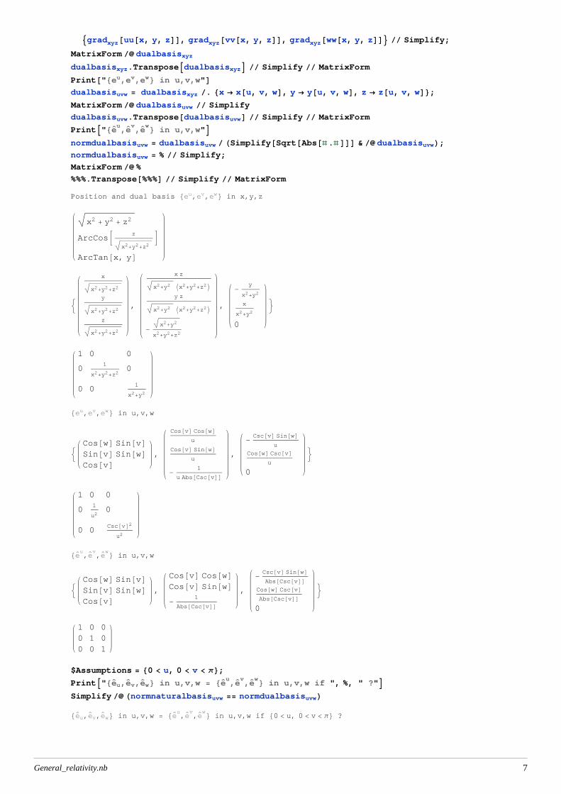
$Assumptions = 80 < u, 0 < v < Π<;PrintA"8eu,ev,ew< in u,v,w = 8eu,ev,ew< in u,v,w if ", %, " ?"ESimplify Hnormnaturalbasisuvw == normdualbasisuvwL8eù,e

`v,e

`w< in u,v,w = 8eù

,e`v,e

`w< in u,v,w if 80 < u, 0 < v < Π< ?


True

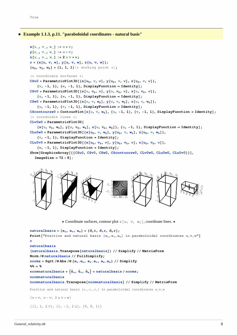
Example 1.1.3, p.11. "paraboloidal coordinates - natural basis"

x@u_, v_, w_D := u + v;

y@u_, v_, w_D := u - v;

z@u_, v_, w_D := 2 u v + w;

r = 8x@u, v, wD, y@u, v, wD, z@u, v, wD<;8u0, v0, w0< = 81, 1, 1<H* working point *L;H* coordinate surfaces *LCSu0 = ParametricPlot3D@8x@u0, v, wD, y@u0, v, wD, z@u0, v, wD<,8v, -1, 1<, 8w, -1, 1<, DisplayFunction ® IdentityD;CSv0 = ParametricPlot3D@8x@u, v0, wD, y@u, v0, wD, z@u, v0, wD<,8u, -1, 1<, 8w, -1, 1<, DisplayFunction ® IdentityD;CSw0 = ParametricPlot3D@8x@u, v, w0D, y@u, v, w0D, z@u, v, w0D<,8u, -1, 1<, 8v, -1, 1<, DisplayFunction ® IdentityD;CScontourzw0 = ContourPlot@z@u, v, w0D, 8u, -1, 1<, 8v, -1, 1<, DisplayFunction ® IdentityD;H* coordinate lines *LCLv0w0 = ParametricPlot3D@8x@u, v0, w0D, y@u, v0, w0D, z@u, v0, w0D<, 8u, -1, 1<, DisplayFunction ® IdentityD;CLu0w0 = ParametricPlot3D@8x@u0, v, w0D, y@u0, v, w0D, z@u0, v, w0D<,8v, -1, 1<, DisplayFunction ® IdentityD;CLu0v0 = ParametricPlot3D@8x@u0, v0, wD, y@u0, v0, wD, z@u0, v0, wD<,8w, -1, 1<, DisplayFunction ® IdentityD;Show@GraphicsArray@88CSu0, CSv0, CSw0, CScontourzw0, CLv0w0, CLu0w0, CLu0v0<<D,

ImageSize ® 72 ´ 8D;00.511.52

00.511.52

-2

0

2

00.511.52 00.511.52

-2-1.5-1-0.50

-2

0

2

-2-1.5-1-0.50

-2-1 0 1 2

-2-1012

-10123

-2-1 0 1 2

-2-1012

-1-0.500.51-1

-0.50

0.51

00.511.52-2-1.5-1-0.5

0

-1

0

1

2

3-2-1.5-1-0.5

0 00.511.5200.511.52

-1

0

1

2

300.511.52

0 1 2 3 4-1-0.500.5111.522.53

0 1 2 3 4

11.522.53

ø Coordinate surfaces, contour plot z@u, v, w0D, coordinate lines. ø

naturalbasis = 8eu, ev, ew< = 8¶ur, ¶vr, ¶wr<;Print@"Position and natural basis 8eu,ev,ew< in paraboloidal coordinates u,v,w"Dr

naturalbasisHnaturalbasis.Transpose@naturalbasisDL Simplify MatrixForm

Norm naturalbasis FullSimplify;

norms = Sqrt Abs 8eu.eu, ev.ev, ew.ew< Simplify

%% %

normnaturalbasis = 9eu, ev, ew= = naturalbasis norms;

normnaturalbasis

normnaturalbasis.Transpose@normnaturalbasisD Simplify MatrixForm

Position and natural basis 8eu,ev,ew< in paraboloidal coordinates u,v,w

8u + v, u - v, 2 u v + w<881, 1, 2 v<, 81, -1, 2 u<, 80, 0, 1<<


2 + 4 v2 4 u v 2 v

4 u v 2 + 4 u2 2 u2 v 2 u 1

: 2 + 4 v2 , 2 + 4 u2 , 1>True

:: 1

2 + 4 v2,

1

2 + 4 v2,

2 v

2 + 4 v2>, : 1

2 + 4 u2, -

1

2 + 4 u2,

2 u

2 + 4 u2>, 80, 0, 1<>

12 u v

I1+2 u2M I1+2 v2M2 v

2+4 v2

2 u v

I1+2 u2M I1+2 v2M1

2 u

2+4 u2

2 v

2+4 v2

2 u

2+4 u21

Exercise 1.1.2 c), p.12-13 "paraboloidal coordinates ( - dual basis)"

Evaluate first Example 1.1.3!

8eu, ev, ew<81, 0, 0< HoldForm@eu 2 + ev 2 - Hu + vL ewD% ReleaseHold

881, 1, 2 v<, 81, -1, 2 u<, 80, 0, 1<<81, 0, 0<

1

281, 1, 2 v< +

1

281, -1, 2 u< - Hu + vL 80, 0, 1<

True

Addendum

Print@"Inverted equations"Dr == 8x, y, z<Solve@%, 8u, v, w<D;8u, v, w< = 8u, v, w< . %@@1DDgradxyz@scalarfield_D := 9¶xscalarfield, ¶yscalarfield, ¶zscalarfield=Print@"Dual basis 8eu,ev,ew< in x,y,z and in paraboloidal coordinates u,v,w"Ddualbasisxyz = 9euxyz, evxyz, ewxyz= = 9gradxyz@uD, gradxyz@vD, gradxyz@wD=;9dualbasisxyz,dualbasisxyz.TransposeAdualbasisxyzE Simplify MatrixForm=

Clear@u, v, wDdualbasisuvw = H* 8eu,ev,ew<= *L8euuvw, evuvw, ewuvw< = dualbasisxyz . 8x ® x@u, v, wD, y ® y@u, v, wD, z ® z@u, v, wD<;8dualbasisuvw,dualbasisuvw.Transpose@dualbasisuvwD Simplify MatrixForm<

Inverted equations

8u + v, u - v, 2 u v + w< 8x, y, z<:x + y

2,x - y

2,1

2I-x2 + y2 + 2 zM>


Dual basis 8eu,ev,ew< in x,y,z and in paraboloidal coordinates u,v,w

:::12,1

2, 0>, : 1

2, -

1

2, 0>, 8-x, y, 1<>,

1

20

1

2H-x + yL

01

2

1

2H-x - yL

1

2H-x + yL 1

2H-x - yL 1 + x2 + y2

>

:::12,1

2, 0>, : 1

2, -

1

2, 0>, 8-u - v, u - v, 1<>,

1

20 -v

01

2-u

-v -u 1 + 2 u2 + 2 v2

>

1.2 Suffix notation p. 13 - 19

FN: "The suffix notation provides a way of handling collections of related quantities that otherwise might be represented by

arrays. The coordinates of a point constitute such a collection, as do the components of a vector, and the vectors on a basis. The

basic idea is to represent the members of such a collection by means of a kernel letter to which is attached a literal suffix (or

suffixes) representing numbers that serve to label the quantities in the collection."

Needs@"TensorCalculus3`Tensorial`"D$PrePrint =.

labs = 8x, ∆, g, G<;DeclareBaseIndices@81, 2, 3<D;Print@"Space dimension: ", NDimDDefineTensorShortcuts@88x, e<, 1<,88∆<, 2<DSetTensorValues@∆ud@i, jD, IdentityMatrix@NDimDD∆ud@i, jD HToArrayValues@D@∆ud@i, jDD MatrixFormLMyRed = StyleForm@Superscript@ð, "¢"D, FontColor ® RGBColor@1, 0, 0DD &;

DeclareIndexFlavor@8red, MyRed<DSpace dimension: 3

∆ ji

1 0 00 1 00 0 1

SetTensorValueRules@xu@iD, 8x@u, v, wD, y@u, v, wD, z@u, v, wD<D8xu@iD, ToArrayValues@D@xu@iDD<8ed@iD, ToArrayValues@D@ed@iDD<8xu@iD ed@iD, EinsteinSum@D@xu@iD ed@iDD, ToArrayValues@D@xu@iD ed@iDD<H%@@2DD . TensorValueRules@xDL %@@3DD9xi, 8x@u, v, wD, y@u, v, wD, z@u, v, wD<=9ei, 9e1, e2, e3==9ei xi, e1 x

1 + e2 x2 + e3 x

3, e1 x@u, v, wD + e2 y@u, v, wD + e3 z@u, v, wD=True

SetTensorValueRules@ed@iD, IdentityMatrix@NDimDDTensorValueRules@eD8xu@iD ed@iD, EinsteinSum@D@xu@iD ed@iDD, ToArrayValues@D@xu@iD ed@iDD<9e1 ® 81, 0, 0<, e2 ® 80, 1, 0<, e3 ® 80, 0, 1<=


9ei xi, e1 x1 + e2 x

2 + e3 x3, 8x@u, v, wD, y@u, v, wD, z@u, v, wD<=

a = xu@iD ed@iD ToArrayValues@D;MatrixForm 8"P", a . 8u ® u0, v ® v0, w ® w0<, "CL", a . 8v ® v0, w ® w0<, a . 8u ® u0, w ® w0<,

a . 8u ® u0, v ® v0<, "CS",

a . u ® u0, a . v ® v0, a . w ® w0, "s", a<:P, x@u0, v0, w0D

y@u0, v0, w0Dz@u0, v0, w0D , CL,

x@u, v0, w0Dy@u, v0, w0Dz@u, v0, w0D ,

x@u0, v, w0Dy@u0, v, w0Dz@u0, v, w0D ,

x@u0, v0, wDy@u0, v0, wDz@u0, v0, wD ,

CS,

x@u0, v, wDy@u0, v, wDz@u0, v, wD ,

x@u, v0, wDy@u, v0, wDz@u, v0, wD ,

x@u, v, w0Dy@u, v, w0Dz@u, v, w0D , s,

x@u, v, wDy@u, v, wDz@u, v, wD >

SetTensorValueRules@xu@rediD, 8u, v, w<D8xu@iD, xu@redjD<ToArrayValues@D %

a = PartialD@xu@jD, rediD;b = a ExpandPartialD@labsD;8a, b, b TraditionalForm, MatrixForm Hb ToArrayValues@DL<:xi, x

j¢ >88x@u, v, wD, y@u, v, wD, z@u, v, wD<, 8u, v, w<<

:x ,i¢j

, ¶xi

¢ xj,

¶xj

¶xi¢, : xH1,0,0L@u, v, wD

yH1,0,0L@u, v, wDzH1,0,0L@u, v, wD

,

xH0,1,0L@u, v, wDyH0,1,0L@u, v, wDzH0,1,0L@u, v, wD

,

xH0,0,1L@u, v, wDyH0,0,1L@u, v, wDzH0,0,1L@u, v, wD

>>

1.3 Tangents and gradients p. 19 - 23

Keywords: tangent vector to a curve, length of a curve, line element HdsL2 in general coordinates, partial differential operator

¶i or ,i.

Sometimes it is more natural to work with the natural basis (example: tangents to curves) and sometimes it is more natural to

work with the dual basis (example: gradients of scalar fields).


ScalarField@x_, y_, z_D = -+1

Hx - 1L2 + Hy - 1L2 + Hz - 1L2

--1

Hx - 1L2 + Hy - 2L2 + Hz - 1L2

;

gSF@x_, y_, z_D = Grad@ScalarField@x, y, zD, Cartesian@x, y, zDD;% MatrixForm

--1+x

IH-1+xL2+H-2+yL2+H-1+zL2M32 +-1+x

IH-1+xL2+H-1+yL2+H-1+zL2M32

--2+y

IH-1+xL2+H-2+yL2+H-1+zL2M32 +-1+y

IH-1+xL2+H-1+yL2+H-1+zL2M32-

-1+z

IH-1+xL2+H-2+yL2+H-1+zL2M32 +-1+z

IH-1+xL2+H-1+yL2+H-1+zL2M32

nmax = 500; s = .15;

rp = Table@2 8Random@D, 3 2 Random@D, Random@D<, 8n, 1, nmax<D;gSFp = gSF@Sequence ð1D & rp;

Table@Graphics3D@8Point@rp@@nDDD,General_relativity.nb 11

8Point@rp@@nDDD,8If@Ha = Norm@ gSFp@@nDDDL < Hb = 5L, Hue@a bD, [email protected],Line@8rp@@nDD, rp@@nDD + s gSFp@@nDD<D<<D,8n, 1, nmax<D;;

Show@%, Axes ® True, AxesLabel ® 8"X", "Y", "Z"<,PlotRange ® 2 880, 1<, 80, 3 2<, 80, 1<<, ViewPoint ® 82, 0, 0<, ImageSize ® 72 ´ 4D;

00.511.5

2

X

0 1 2 3

Y

0

0.5

1

1.5

2

Z

0

0.5

1

1.5

2

Z

ø Gradient of the 3D scalar field at random points. ø

Exercise 1.3.3, p.23.

Show that if the arc-length s (measured along a curve from some base point) is used as a parameter, then at each point of the

curve given by Ξ(s) the tangent vector d Ξ(s) / ds has unit length.

Solution by David Park:

Hâ sL2 gi j â xi â xj, 1 gi j

âxi

âs

âxj

âs;

Ξ ei xi,âΞ

âs ei

âxi

âs

âΞ

âs

2

ei

âxi

âs. e j

âxj

âs

âΞ

âs

2

gi j

âxi

âs

âxj

âs

âΞ

âs

2

1,âΞ

âs 1 q.e.d .

1.4 Coordinate transformations in Euclidean space p. 23 - 27

FN: "The purpose of this section is to explain how such things as the components of vectors relative to the bases defined by the

coordinate systems transform, when we pass from the unprimed to the primed coordinate system (or vice versa). To this end, we

shall use the suffix notation [...]."

Be careful:


:a b , a2 b > . 8a ® -1, b ® +1<9DtAs2E, HDt@sDL2, Dt@sD2, d s2, ds2= TraditionalForm

8-1, 1<92 s â s, Hâ sL2, Hâ sL2, d s2, ds2=

Example 1.4.1, p.25.

Mathematica: spherical coordinates: Rr Cos[Pphi] Sin[Ttheta], Rr Sin[Pphi] Sin[Ttheta], Rr Cos[Ttheta], Rr, Ttheta, Pphi, 0 £ Rr < ¥,

0 £ Ttheta £ Π, -Π < Pphi £ Π;

cylindrical coordinates: Rr Cos[Ttheta], Rr Sin[Ttheta], Zz, Rr, Ttheta, Zz, 0 £ Rr < ¥, -Π < Ttheta £ Π, -¥ < Zz <¥.

8x, y, z< 8r Sin@ΘD Cos@ΦD, r Sin@ΘD Sin@ΦD, r Cos@ΘD< 8Ρ Cos@ΦD, Ρ Sin@ΦD, z<;Drop@%, 1D Thread

8r Cos@ΦD Sin@ΘD Ρ Cos@ΦD, r Sin@ΘD Sin@ΦD Ρ Sin@ΦD, r Cos@ΘD z<Transformation between spherical coordinates and cylindrical coordinates :

Hin = :r ® Ρ2 + z2 , Θ ® ArcTan@Ρ zD, Φ ® Φ>;

Her = 8Ρ ® r Sin@ΘD, Φ ® Φ, z ® r Cos@ΘD< ;

88HerVar, HerTrans<, 8HinVar, HinTrans<< = 8Table@Hð . Rule ® ListL@@i, 1DD, 8i, 3<D,Table@Hð . Rule ® ListL@@i, 2DD, 8i, 3<D< & 8Hin, Her<

Us = Outer@D@ð1, ð2D &, HinTrans, HerVar, 1D;Uc = Simplify@Us . Hin, 8z ³ 0<D;Uc`

= Outer[D[#1, ð2F &, HerTrans, HinVar, 1F Simplify;

Us`

= Simplify[Uc` . Her, r ³ 0F;

MatrixForm :Us, Uc, Uc`, Us

` >MatrixForm :Us.Us` , Uc.Uc

` > Simplify

::8r, Θ, Φ<, : z2 + Ρ2 , ArcTanB Ρ

zF, Φ>>, 88Ρ, Φ, z<, 8r Sin@ΘD, Φ, r Cos@ΘD<<>

: Sin@ΘD r Cos@ΘD 00 0 1Cos@ΘD -r Sin@ΘD 0

,

Ρ

z2+Ρ2z 0

0 0 1z

z2+Ρ2-Ρ 0

,

Ρ

z2+Ρ20

z

z2+Ρ2

z

z2+Ρ20 -

Ρ

z2+Ρ2

0 1 0

,

Sin@ΘD 0 Cos@ΘDCos@ΘD

r0 -

Sin@ΘDr

0 1 0

>

: 1 0 00 1 00 0 1

,1 0 00 1 00 0 1

>From Exercise 1.1.2 the unit vector field Λ = i has the spherical contravariant components:


Lss = 8Sin@ΘD Cos@ΦD, Cos@ΘD Cos@ΦD r, -Csc@ΘD Sin@ΦD r<;Lsc = Simplify@Lss . Hin, 8z ³ 0<D;Lcs = Us.Lss Simplify;

Lcc = Simplify@Lcs . Hin, 8z ³ 0<D;MatrixForm 8Lss, Lsc, Lcs, Lcc<:Lsc == Uc

`.Lcc, Lss Simplify@Lsc . Her, r ³ 0D,

Lcc == [email protected], Lss == Us`.Lcs, Lcs Lcc . Her>

:Cos@ΦD Sin@ΘDCos@ΘD Cos@ΦD

r

-Csc@ΘD Sin@ΦD

r

,

Ρ Cos@ΦDz2+Ρ2

z Cos@ΦDz2+Ρ2

-Sin@ΦD

Ρ

,

Cos@ΦD-

Csc@ΘD Sin@ΦDr

0

,

Cos@ΦD-

Sin@ΦDΡ

0

>

8True, True, True, True, True<


[...] Hence, using G from Example 1.3.1 and U`

from Example 1.4.1, obtain the line element for Euclidean space in cylindrical

coordinates.

The contracted dummy indices have to be brought adjacent. But where they are not adjacent we must use a transpose.

Gss = DiagonalMatrixA91, r2, r2 Sin@ΘD2=E;Gsc = Gss . Hin Simplify;

MatrixForm 8Gss, Gsc<Dt@sD2 == [email protected]@HerVarD TraditionalForm

Print@"line element for Euclidean space in spherical coordinates"D: 1 0 0

0 r2 0

0 0 r2 Sin@ΘD2

,

1 0 0

0 z2 + Ρ2 0

0 0 Ρ2

>

Hâ sL2 Hâ rL2 + r2 Hâ ΘL2 + r2 Hâ ΦL2 sin2HΘLline element for Euclidean space in spherical coordinates

Gcs = Transpose@Us` D.Gss.Us` Simplify;

Gcc = Gcs . Hin Simplify;

MatrixForm 8Gcs, Gcc<Dt@sD2 == [email protected]@HinVarD TraditionalForm

Print@"line element for Euclidean space in cylindrical coordinates"D: 1 0 0

0 r2 Sin@ΘD2 0

0 0 1

,

1 0 0

0 Ρ2 0

0 0 1

>Hâ sL2 Hâ zL2 + Hâ ΡL2 + Ρ2 Hâ ΦL2

line element for Euclidean space in cylindrical coordinates


1.5 Tensor fields in Euclidean space p. 27 - 30

FN: "While scalar and vector fields are sufficient to formulate Newton's theory of gravitation, tensor fields are an additional

requirement for Einstein's theory."

Note: Often the label L instead of the Foster and Nightingale U is used to represent the transformation matrices.

The general rule for transforming tensors is just to use a transformation matrix L (Jacobian matrix) for each index in the tensor.

The L matrix always has the ud configuration and has indices of different flavors. The dummy indices must be matched to the

old indices and the other indices must correspond to the new free indices.

Example: Τ j¢i¢

L j¢l

L ki¢

Τ lk

Needs@"TGeneralRelativity1`GeneralRelativity`"D$PrePrint =.

DeclareBaseIndices@81, 2, 3<DDefineTensorShortcuts@88e, f, n<, 1<,88g, L, Τ<, 2<DMyRed = StyleForm@Superscript@ð, "¢"D, FontColor ® RGBColor@1, 0, 0DD &;

DeclareIndexFlavor@8red, MyRed<DThe force-stress-relation f

Ó = Τ ( nÓ ) in component form:

Print@"Vector representation of forces"Dfu@iD ed@iD Τ@nu@jD ed@jDDPrint@"Τ is linear on the basis vectors"D%% LinearBreakout@ΤD@ed@_DDPrint@"Expand Τ on the basis vectors"D%% . Τ@ed@jDD ® Τud@i, jD ed@iDPrint@"We obtain the force components:"DHð ed@iD & %%L FrameBox DisplayForm

Vector representation of forces

ei fi ΤBej njF

Τ is linear on the basis vectors

ei fi n

jΤBejF

Expand Τ on the basis vectors

ei fi ei n

jΤ ji

We obtain the force components:

fi nj

Τ ji


Show that the components Τ ji of the stress tensor Τ are given by Τ j

i ei.Τ IejMand use this result to re-establish the

transformation formula (1.58) for the components. General_relativity.nb 15

Show that the components Τ ji of the stress tensor Τ are given by Τ j

i ei.Τ IejMand use this result to re-establish the

transformation formula (1.58) for the components.

Hstep1 = Τud@i, jD == eu@iD.Τ@ed@jDDL FrameBox DisplayForm

PrintA"Expand Τ"Estep1 . Τ@ed@jDD ® Τud@k, jD ed@kDPrint@"Linearity of dot product"D%% LinearBreakout@DotD@ed@_DDPrint@"Basis, dual basis relation and using g as a Kronecker"D%% . BasisDotProductRules@e, gD% KroneckerAbsorb@gD

Τ ji

ei.ΤBejFExpand Τ

Τ ji

ei.Jek Τ jk N

Linearity of dot product

Τ ji

ei.ek Τ jk

Basis, dual basis relation and using g as a Kronecker

Τ ji

g ki Τ j

k

True

We can now use this to establish the transformation relation:

Print@"We turn step1 into a rule."Drule1 = Rule Reversestep1 LHSSymbolsToPatterns@8i, j<Dstep1 ToFlavor@redDPrint@"Express red basis vectors in terms of plain coordinates"D%% . eu@rediD ® Lud@redi, kD eu@kD . ed@redjD ® Lud@l, redjD ed@lDPrint@"Use linearity of Τ and dot product"D%% LinearBreakout@Dot, ΤD@ed@_D, eu@_D, Τ@_DDPrint@"Use previous relation to substitute Τ components"D%% . rule1

We turn step1 into a rule.

ei_.ΤBej_F ® Τ j

i

Τ j¢i¢

ei¢.ΤBej¢ F

Express red basis vectors in terms of plain coordinates

Τ j¢i¢

Iek L ki¢ M.ΤBel L j¢

l FUse linearity of Τ and dot product

Τ j¢i¢

ek.ΤAelE L j¢l

L ki¢

Use previous relation to substitute Τ components

Τ j¢i¢

L j¢l

L ki¢

Τ lk

This is the desired transformation relation.


This is the desired transformation relation.

1.6 Surfaces in Euclidean space p. 30 - 35

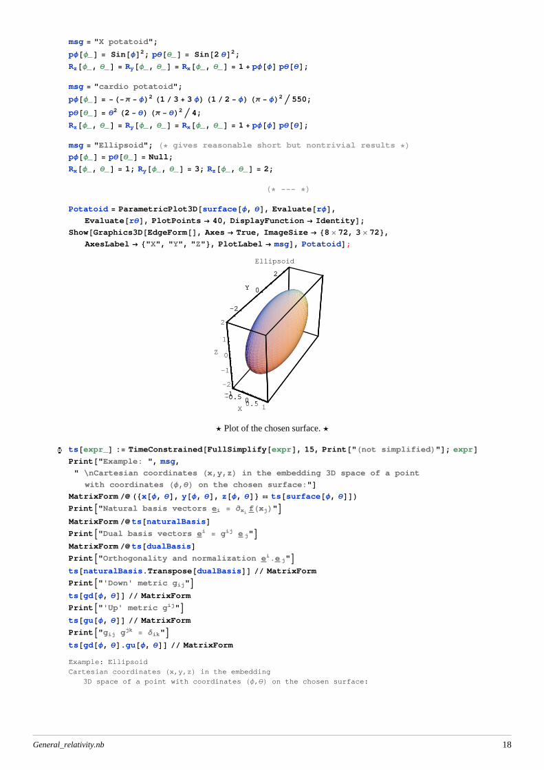
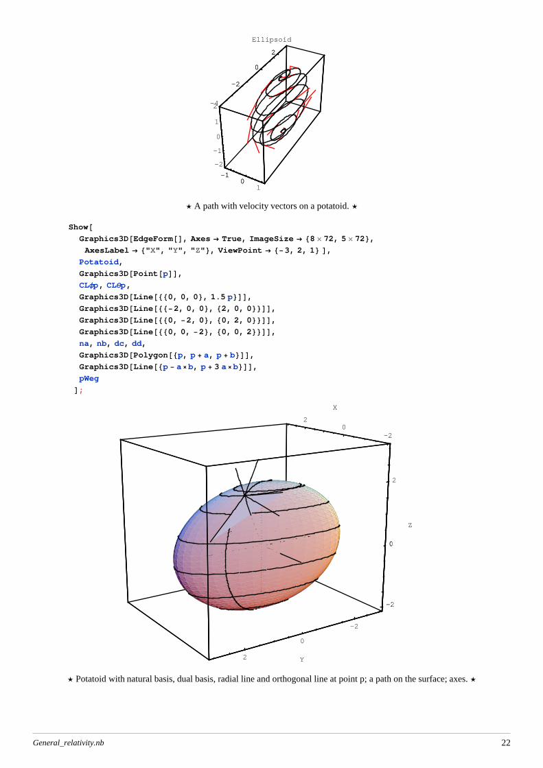
The Potatoid Project- A project for doing geometry on potatoids -

It's nice to play around with all the new geometrical concepts (coordinate transformations, natural basis, metric, dual basis,

geodetics, parallel transport, etc.) in a nontrivial context where a complete visual representation is still possible. Sufficiently

smooth and well-behaved deformations of a spherical surface (2D) embedded in a regular 3D Euclidean space (which I call

potatoids) provide such a "geometrical playground". The basic coordinate system (Φ, Θ) on potatoids is borrowed from spherical

coordinates on the sphere.

Spherical coordinates in Mathematica

Rr Cos[Pphi] Sin[Ttheta], Rr Sin[Pphi] Sin[Ttheta], Rr Cos[Ttheta], Rr, Ttheta, Pphi, 0 £ Rr < ¥, 0 £ Ttheta £ Π, -Π <

Pphi £ Π.

$Assumptions = -Π < Φ £ Π && 0 £ Θ £ Π;

rΦ = 8Φ, -Π, Π<; rΘ = 8Θ, 0, Π<;surface@Φ_, Θ_D = 9

Rx@Φ, ΘD Cos@ΦD Sin@ΘD,Ry@Φ, ΘD Sin@ΦD Sin@ΘD,Rz@Φ, ΘD Cos@ΘD=;

naturalBasis = 8nb1@Φ_, Θ_D, nb2@Φ_, Θ_D< = 8D@surface@Φ, ΘD, ΦD, D@surface@Φ, ΘD, ΘD<;H*'down' metric *Lgd@Φ_, Θ_D = naturalBasis.Transpose@naturalBasisD;H*'up' metric *Lgu@Φ_, Θ_D = Inverse@gd@Φ, ΘDD;dualBasis = 8db1@Φ_, Θ_D, db2@Φ_, Θ_D< = gu@Φ, ΘD.naturalBasis;angleBetweenNaturalBasisVectors@Φ_, Θ_D =

ArcCosAgd@Φ, ΘD@@1,2DD HNorm@nb1@Φ, ΘDD Norm@nb2@Φ, ΘDDLE Pi * 180;H* a path on the surface parametrized by t *Lpath@t_D = surface@fΦ@tD, fΘ@tDD;velocity@t_D = gd@fΦ@tD, fΘ@tDD@@1,1DD fΦ'@tD2 +

2 gd@fΦ@tD, fΘ@tDD@@1,2DD fΦ'@tD fΘ'@tD +

gd@fΦ@tD, fΘ@tDD@@2,2DD fΘ'@tD2

;

length@ti_, tf_D := àti

tf

velocity@tD ât;

Nlength@ti_, tf_D := NIntegrate@velocity@tD, 8t, ti, tf<D;H* A little collection of potatoids: *L

msg = "sphere";

pΦ@Φ_D = pΘ@Θ_D = 0;

Rz@Φ_, Θ_D = Ry@Φ_, Θ_D = Rx@Φ_, Θ_D = 1 + pΦ@ΦD pΘ@ΘD;msg = "shell potatoid";H* interesting, but NOT well behaved *LpΦ@Φ_D = H-Π - ΦL2; pΘ@Θ_D = 1;

Rz@Φ_, Θ_D = Ry@Φ_, Θ_D = Rx@Φ_, Θ_D = 1 + pΦ@ΦD pΘ@ΘD;


msg = "X potatoid";

pΦ@Φ_D = Sin@ΦD2; pΘ@Θ_D = Sin@2 ΘD2;

Rz@Φ_, Θ_D = Ry@Φ_, Θ_D = Rx@Φ_, Θ_D = 1 + pΦ@ΦD pΘ@ΘD;msg = "cardio potatoid";

pΦ@Φ_D = -H-Π - ΦL2 H1 3 + 3 ΦL H1 2 - ΦL HΠ - ΦL2 550;

pΘ@Θ_D = Θ2 H2 - ΘL HΠ - ΘL2 4;

Rz@Φ_, Θ_D = Ry@Φ_, Θ_D = Rx@Φ_, Θ_D = 1 + pΦ@ΦD pΘ@ΘD;msg = "Ellipsoid"; H* gives reasonable short but nontrivial results *LpΦ@Φ_D = pΘ@Θ_D = Null;

Rx@Φ_, Θ_D = 1; Ry@Φ_, Θ_D = 3; Rz@Φ_, Θ_D = 2;

H* --- *LPotatoid = ParametricPlot3D@surface@Φ, ΘD, Evaluate@rΦD,

Evaluate@rΘD, PlotPoints ® 40, DisplayFunction ® IdentityD;Show@Graphics3D@EdgeForm@D, Axes ® True, ImageSize ® 88 ´ 72, 3 ´ 72<,

AxesLabel ® 8"X", "Y", "Z"<, PlotLabel ® msgD, PotatoidD;Ellipsoid

-1-0.5 00.5 1X

-2

0

2

Y

-2

-1

0

1

2

Z

-1-0.5 00.5 1X

-2

0

2

Y

ø Plot of the chosen surface. ø

Ý ts@expr_D := TimeConstrained@FullSimplify@exprD, 15, Print@"Hnot simplifiedL"D; exprDPrint@"Example: ", msg,

" \nCartesian coordinates Hx,y,zL in the embedding 3D space of a point

with coordinates HΦ,ΘL on the chosen surface:"DMatrixForm H8x@Φ, ΘD, y@Φ, ΘD, z@Φ, ΘD< ts@surface@Φ, ΘDDLPrintA"Natural basis vectors ei = ¶xi fHxjL"EMatrixForm ts@naturalBasisDPrintA"Dual basis vectors ei = gij e j"EMatrixForm ts@dualBasisDPrintA"Orthogonality and normalization ei.e j"[email protected]@dualBasisDD MatrixForm

PrintA"'Down' metric gij"Ets@gd@Φ, ΘDD MatrixForm

PrintA"'Up' metric gij"Ets@gu@Φ, ΘDD MatrixForm

PrintA"gij gjk = ∆ik"Ets@gd@Φ, ΘD.gu@Φ, ΘDD MatrixForm

Example: Ellipsoid

Cartesian coordinates Hx,y,zL in the embedding

3D space of a point with coordinates HΦ,ΘL on the chosen surface:


x@Φ, ΘDy@Φ, ΘDz@Φ, ΘD

Cos@ΦD Sin@ΘD3 Sin@ΘD Sin@ΦD2 Cos@ΘD

Natural basis vectors ei = ¶xifHxjL

: -Sin@ΘD Sin@ΦD3 Cos@ΦD Sin@ΘD0

,Cos@ΘD Cos@ΦD3 Cos@ΘD Sin@ΦD-2 Sin@ΘD >

Dual basis vectors ei = gij e j

:H13+5 Cos@2 ΘDL Csc@ΘD Sin@ΦD

-29+11 Cos@2 ΘD-32 Cos@2 ΦD Sin@ΘD23 H-5+3 Cos@2 ΘDL Cos@ΦD Csc@ΘD

-29+11 Cos@2 ΘD-32 Cos@2 ΦD Sin@ΘD2-

16 Cos@ΘD Sin@2 ΦD-29+11 Cos@2 ΘD-32 Cos@2 ΦD Sin@ΘD2

,

18 Cos@ΘD Cos@ΦD29-11 Cos@2 ΘD+32 Cos@2 ΦD Sin@ΘD2-

6 Cos@ΘD Sin@ΦD-29+11 Cos@2 ΘD-32 Cos@2 ΦD Sin@ΘD2

-4 H5+4 Cos@2 ΦDL Sin@ΘD

29-11 Cos@2 ΘD+32 Cos@2 ΦD Sin@ΘD2>

Orthogonality and normalization ei.e j

K 1 00 1

O'Down' metric gij

H5 + 4 Cos@2 ΦDL Sin@ΘD2 8 Cos@ΘD Cos@ΦD Sin@ΘD Sin@ΦD8 Cos@ΘD Cos@ΦD Sin@ΘD Sin@ΦD Cos@ΘD2 H5 - 4 Cos@2 ΦDL + 4 Sin@ΘD2

'Up' metric gij

8+H10-8 Cos@2 ΦDL Cot@ΘD229-11 Cos@2 ΘD+32 Cos@2 ΦD Sin@ΘD2

8 Cot@ΘD Sin@2 ΦD-29+11 Cos@2 ΘD-32 Cos@2 ΦD Sin@ΘD2

8 Cot@ΘD Sin@2 ΦD-29+11 Cos@2 ΘD-32 Cos@2 ΦD Sin@ΘD2

2 H5+4 Cos@2 ΦDL29-11 Cos@2 ΘD+32 Cos@2 ΦD Sin@ΘD2

gij gjk = ∆ik

K 1 00 1

Op1 = Plot@pΦ@ΦD, Evaluate@rΦD, AxesLabel ® 8"Φ", "pΦ@ΦD"<,

PlotStyle ® Hue@0D, DisplayFunction ® IdentityD;p2 = Plot@pΘ@ΘD, Evaluate@rΘD, AxesLabel ® 8"Θ", "pΘ@ΘD"<,

PlotStyle ® Hue@0D, DisplayFunction ® IdentityD;p3 = Plot3D@Norm@surface@Φ, ΘDD, Evaluate@rΦD, Evaluate@rΘD,

Mesh ® True, PlotRange ® 8Rest@rΦD, Rest@rΘD, 80.5, 2<<,AxesLabel ® 8"Φ", "Θ", "r@Φ,ΘD "<, DisplayFunction ® IdentityD;

Show@GraphicsArray@8p1, p2, p3<D, ImageSize ® 72 ´ 8D;

0.2 0.4 0.6 0.8 1Φ

0.2

0.4

0.6

0.8

1pΦ@ΦD

0.2 0.4 0.6 0.8 1Θ

0.2

0.4

0.6

0.8

1pΘ@ΘD

-20

2Φ 0

1

23

Θ0.51

1.52

r@Φ,ΘD-2

02Φ

ø Functions pΦ(Φ) and pΘ(Θ) if defined. Radial coordinate r(Φ, Θ) of the point (Φ, Θ). ø

Ε = 90, 10-6, -10-6=;p1 = Plot3D@angleBetweenNaturalBasisVectors@Φ, ΘD, Evaluate@rΦ + ΕD, Evaluate@rΘ + ΕD,

Mesh ® True, PlotRange ® 8Rest@rΦD, Rest@rΘD, Automatic<, AxesLabel ® 8"Φ", "Θ", ""<,PlotLabel ® "ÐHe1, e2L in °", DisplayFunction ® IdentityD;

p2 = ContourPlot@angleBetweenNaturalBasisVectors@Φ, ΘD,, , ,


p2 = ContourPlot@angleBetweenNaturalBasisVectors@Φ, ΘD,Evaluate@rΦ + ΕD, Evaluate@rΘ + ΕD, PlotRange ® 8Rest@rΦD, Rest@rΘD, Automatic<,PlotPoints ® 50, FrameLabel ® 8"Φ", "Θ"<, DisplayFunction ® IdentityD;

Show@GraphicsArray@8p1, p2<D, ImageSize ® 72 ´ 6D;ÐHe1, e2L in °

-20

2Φ0

1

2

3

Θ

5075

100125

-20

2Φ -3 -2 -1 0 1 2 3Φ

0.5

1

1.5

2

2.5

3

Θ

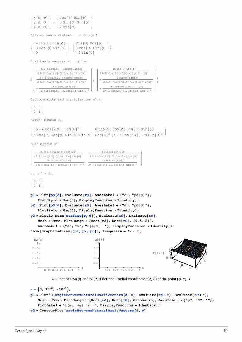
ø Angle between natural basis vectors at point (Φ, Θ). ø

H* working point p *LΦp = 2.5; Θp = 0.5 ;

p = surface@Φp, ΘpD N

8-0.384089, 0.860768, 1.75517<H* natural basis and properties at point p *La = nb1@Φp, ΘpD N; na = Graphics3D@Line@8p, p + a<DD;b = nb2@Φp, ΘpD N; nb = Graphics3D@Line@8p, p + b<DD;8a MatrixForm, b MatrixForm, Norm@aD, Norm@bD, a.b,

a.b HNorm@aD Norm@bDL, angleBetweenNaturalBasisVectors@Φp, ΘpD "°"<: -0.286923

-1.152270.

,-0.703071.57563-0.958851

, 1.18745, 1.9739, -1.61381, -0.688512, 133.512 °>H* down metric, up metric and their product at point p *LMatrixForm N@8gd@Φp, ΘpD, gu@Φp, ΘpD, gd@Φp, ΘpD.gu@Φp, ΘpD<D:K 1.41004 -1.61381

-1.61381 3.8963O, K 1.34841 0.5585

0.5585 0.48798O, 1. 3.17671 ´ 10-17

9.21572 ´ 10-17 1.>

H* dual basis and properties at point p *Lc = db1@Φp, ΘpD N; dc = Graphics3D@Line@8p, p + c<DD;d = db2@Φp, ΘpD N; dd = Graphics3D@Line@8p, p + d<DD;8c MatrixForm, d MatrixForm, Norm@cD, Norm@dD, c.d,

c.d HNorm@cD Norm@dDL, H180 - [email protected] HNorm@cD Norm@dDLD Pi * 180L "°"<88a.c, a.d<, 8b.c, b.d<< MatrixForm

: -0.779554-0.67374-0.535518

,-0.503330.125333-0.4679

, 1.16121, 0.698555, 0.5585, 0.688512, 133.512 °>1. -1.38791 ´ 10-16

2.17491 ´ 10-16 1.

CLΦp = ParametricPlot3D@surface@Φp, ΘD, Evaluate@rΘD, DisplayFunction ® IdentityD;CLΘp = ParametricPlot3D@surface@Φ, ΘpD, Evaluate@rΦD, DisplayFunction ® IdentityD;Show@CLΦp, CLΘp, na, nb, dc, dd, DisplayFunction ® $DisplayFunction,

AxesLabel ® 8"X", "Y", "Z"<, ImageSize ® 88 ´ 72, 3 ´ 72<, ViewPoint ® 5 H p + 8.2, .3, .5<LD;


-1-0.500.5X

-1

0

1

2

Y

-2

-1

0

1

2

Z

-1

0

1

2

Y

-2

-1

0

1

2

Z

ø Coordinate lines, natural basis and dual basis at point p. ø

H* Straight path from north pole to south pole, 0£t£1 *LfΦ@t_D := Π

fΘ@t_D := Π t

nr = 1;

H* Spiral path from north pole to south pole with nr spires, 0£t£1 *Lnr = 7;

fΦ@t_D := -Π + Mod@2 Π nr t, 2 ΠDfΘ@t_D := Π t

H* Path length analyticalnumerical *LTimeConstrained@length@0, 1D, 10DTimeConstrained@Nlength@0, 1D, 20D$Aborted

75.2417

H* At a particular point of the path *Lpt = 0.4;

MatrixForm 88Φpt = fΦ@ptD, Θpt = fΘ@ptD<,8apt = fΦ'@ptD, bpt = fΘ'@ptD<, apt nb1@Φpt, ΘptD + bpt nb2@Φpt, ΘptD<MatrixForm 8path@ptD, path'@ptD<%%@@3DD %@@2DD:K 1.88496

1.25664O, K 43.9823

ΠO, -40.0824

-36.0083-5.97566

>

: -0.2938932.713530.618034

,-40.0824-36.0083-5.97566

>True

pWeg = ParametricPlot3D@path@tD, 8t, 0, 1<, PlotPoints ® nr 75, DisplayFunction ® IdentityD;pvt@t_D = Graphics3D@8Hue@0D, Line@8path@tD, path@tD + path'@tD 50<D<D;Show@pWeg, N@Table@pvt@1 20 nD, 8n, 0, 20<DD,

DisplayFunction ® $DisplayFunction, ImageSize ® 88 ´ 72, 3 ´ 72<, PlotLabel ® msgD;


Ellipsoid

-10

1

-4

-2

0

2

-2

-1

0

1

2

-10

1

-4

-2

0

2

ø A path with velocity vectors on a potatoid. ø

Show@Graphics3D@EdgeForm@D, Axes ® True, ImageSize ® 88 ´ 72, 5 ´ 72<,AxesLabel ® 8"X", "Y", "Z"<, ViewPoint ® 8-3, 2, 1< D,

Potatoid,

Graphics3D@Point@pDD,CLΦp, CLΘp,

Graphics3D@Line@880, 0, 0<, 1.5 p<DD,Graphics3D@Line@88-2, 0, 0<, 82, 0, 0<<DD,Graphics3D@Line@880, -2, 0<, 80, 2, 0<<DD,Graphics3D@Line@880, 0, -2<, 80, 0, 2<<DD,na, nb, dc, dd,

Graphics3D@Polygon@8p, p + a, p + b<DD,Graphics3D@Line@8p - ab, p + 3 ab<DD,pWegD;

-20

2

X

-2

0

2 Y

-2

0

2

Z

-2

0

2

Z

ø Potatoid with natural basis, dual basis, radial line and orthogonal line at point p; a path on the surface; axes. ø


Export@"C:\\USERS\\LUMA\\Mathematica\\_Tensorrechnung\\1.6 - Potatoid_plus.dxf", %, "DXF"D

C:\USERS\LUMA\Mathematica\_Tensorrechnung\1.6 - Potatoid_plus.dxf

"Well, this was instructive but at some point we will have to learn how to do this without the embedding space."

1.7 Manifolds p. 35-37

coming soon...

1.8 Tensor Fields on manifolds p. 38 - 43"We can create new tensors from old tensors by a number of methods."

coming soon...

1.9 Metric properties p. 43 - 46 (pseudo-Riemannian manifolds)

coming soon...

1.10 What and where are the bases? p. 46 - 49

coming soon...

Chapter 2: The spacetime of general relativity and paths of particles

2.0 Introduction p. 53 - 56

FN: "The mathematics of geodesics is covered in the next few sections, along with the related concepts of parallelism and

absolute and covariant differentiation [...]. Note that in the present chapter we are concerned only with the motion of particles in

a given spacetime [...]. How that field arises is answered in the next chapter, where we relate the curvature of spacetime to the

sources of the gravitational field."

"The surface of a cylinder does not have curvature. Therefore, initially parallel geodesics would not deviate from one another.

The ants could not decide if they were on a cylinder or a flat plane simply by examining their geodesics." (David Park)


2.1 Geodesics p. 56 - 64


DeclareBaseIndices@81, 2, 3, 4<Dlabs = 8x, ∆, g, G<;DefineTensorShortcuts@88x, e, Λ, u, zero<, 1<,88∆, g<, 2<,88G<, 3<DDeclareZeroTensor@zeroD$Assumptions = -Π < Φ £ Π && 0 £ Θ £ Π;

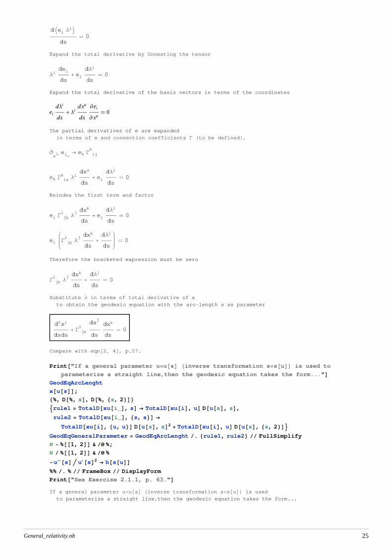
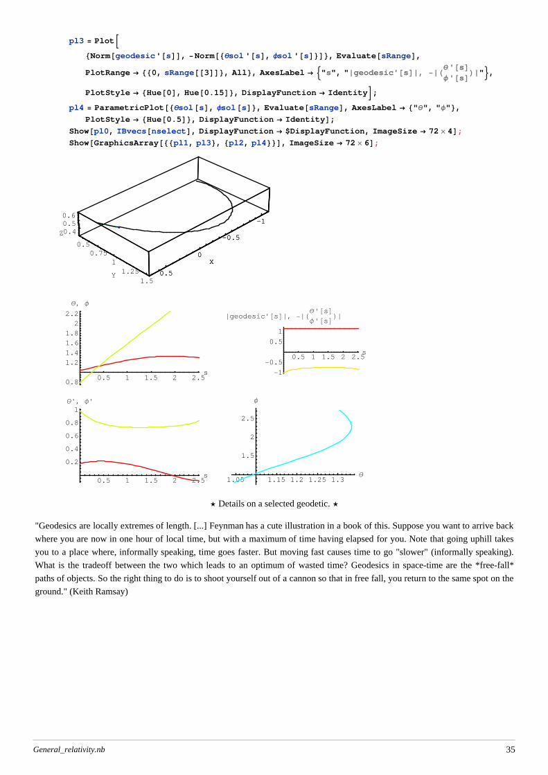
1) Derivation of the affinely parametrized geodesic equation in Euclidean space using the straightness concept. General parametrization.

Print@"For a straight line xHuL all the tangent vectors ΛHuL point in the same direction.

If we use the arc-length s as a parameter u, then the tangent vector is"DΛ TotalD@x, sD TraditionalForm

Print@"Constant direction of tangent vector implies"DTotalD@NestedTensor@ΛD, sD 0

Print@"Substitute component expression for Λ"D%% . Λ ® Λu@iD ed@iDPrint@"Expand the total derivative by Unnesting the tensor"D%% UnnestTensor

Print@"Expand the total derivative of the basis vectors in terms of the coordinates"DMapAt@ExpandTotalD@labs, aD, %%, 881, 1<<D TraditionalForm

Print@"The partial derivatives of e are expanded

in terms of e and connection coefficients G Hto be definedL, "DPartialD@labsD@ed@i_D, xu@j_DD ® Gudd@k, i, jD ed@kD%%% . PartialD@labsD@ed@i_D, xu@j_DD ® Gudd@k, i, jD ed@kDPrint@"Reindex the first term and factor"DMapAt@IndexChange@88k, i<, 8i, j<, 8a, k<<D, %%, 1DMapAt@Factor, %, 1DPrint@"Therefore the bracketed expression must be zero"DMapAt@Rest, %%, 1DPrint@"Substitute Λ in terms of total derivative of x to

obtain the geodesic equation with the arc-length s as parameter"DGeodEqArcLenght = %% . Λu@i_D ® TotalD@xu@iD, sD;% FrameBox DisplayForm

Print@"Compare with eqn@2, 4D, p.57."DFor a straight line xHuL all the tangent vectors ΛHuL point in the same

direction. If we use the arc-length s as a parameter u, then the tangent vector is

Λ â x

â s

Constant direction of tangent vector implies

âΛ

âs 0

Substitute component expression for Λ


âIei ΛiMâs

0

Expand the total derivative by Unnesting the tensor

Λiâei

âs+ ei

âΛi

âs 0

Expand the total derivative of the basis vectors in terms of the coordinates

ei

âΛi

âs+ Λi

âxa

âs

¶ei

¶ xa 0

The partial derivatives of e are expanded

in terms of e and connection coefficients G Hto be definedL,¶xj_ ei_ ® ek G ij

k

ek G iak Λi

âxa

âs+ ei

âΛi

âs 0

Reindex the first term and factor

ei G jki

Λj âxk

âs+ ei

âΛi

âs 0

ei G jki

Λj âxk

âs+

âΛi

âs 0

Therefore the bracketed expression must be zero

G jki

Λj âxk

âs+

âΛi

âs 0

Substitute Λ in terms of total derivative of x

to obtain the geodesic equation with the arc-length s as parameter

â2xi

âsâs+ G jk

iâx

j

âs

âxk

âs 0

Compare with eqn@2, 4D, p.57.

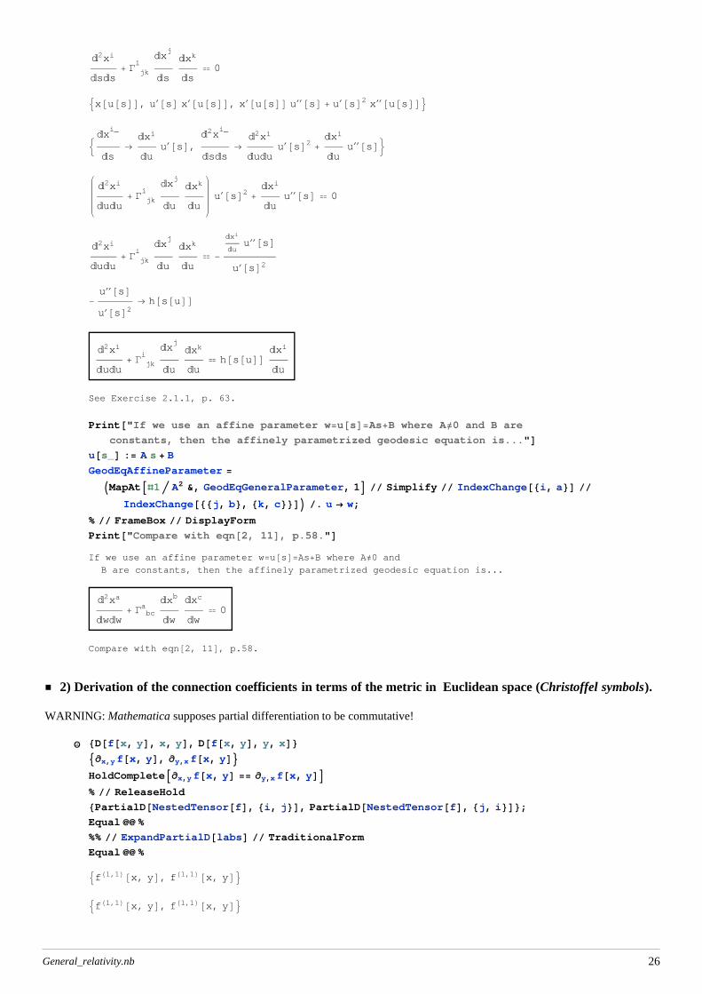
Print@"If a general parameter u=u@sD Hinverse transformation s=s@uDL is used to

parameterize a straight line,then the geodesic equation takes the form..."DGeodEqArcLenght

x@u@sDD;8%, D@%, sD, D@%, 8s, 2<D<9rule1 = TotalD@xu@i_D, sD ® TotalD@xu@iD, uD D@u@sD, sD,rule2 = TotalD@xu@i_D, 8s, s<D ®

TotalD@xu@iD, 8u, u<D D@u@sD, sD2 + TotalD@xu@iD, uD D@u@sD, 8s, 2<D=GeodEqGeneralParameter = GeodEqArcLenght . 8rule1, rule2< FullSimplify

ð - %@@1, 2DD & %;

ð %@@1, 2DD & %

-u¢¢@sD u¢@sD2 ® h@s@uDD%% . % FrameBox DisplayForm

Print@"See Exercise 2.1.1, p. 63."DIf a general parameter u=u@sD Hinverse transformation s=s@uDL is used

to parameterize a straight line,then the geodesic equation takes the form...


â2xi

âsâs+ G jk

iâx

j

âs

âxk

âs 0

9x@u@sDD, u¢@sD x¢@u@sDD, x¢@u@sDD u¢¢@sD + u¢@sD2 x¢¢@u@sDD=: âx

i_

âs®

âxi

âuu¢@sD, â2x

i_

âsâs®

â2xi

âuâuu¢@sD2 +

âxi

âuu¢¢@sD>

â2xi

âuâu+ G jk

iâx

j

âu

âxk

âuu¢@sD2 +

âxi

âuu¢¢@sD 0

â2xi

âuâu+ G jk

iâx

j

âu

âxk

âu -

âxi

âuu¢¢@sD

u¢@sD2

-u¢¢@sDu¢@sD2

® h@s@uDD

â2xi

âuâu+ G jk

iâx

j

âu

âxk

âu h@s@uDD âxi

âu

See Exercise 2.1.1, p. 63.

Print@"If we use an affine parameter w=u@sD=As+B where A¹0 and B are

constants, then the affinely parametrized geodesic equation is..."Du@s_D := A s + B

GeodEqAffineParameter =IMapAtAð1 A2 &, GeodEqGeneralParameter, 1E Simplify IndexChange@8i, a<D IndexChange@88j, b<, 8k, c<<DM . u ® w;

% FrameBox DisplayForm

Print@"Compare with eqn@2, 11D, p.58."DIf we use an affine parameter w=u@sD=As+B where A¹0 and

B are constants, then the affinely parametrized geodesic equation is...

â2xa

âwâw+ G bc

aâxb

âw

âxc

âw 0


2) Derivation of the connection coefficients in terms of the metric in Euclidean space (Christoffel symbols).

WARNING: Mathematica supposes partial differentiation to be commutative!

Î 8D@f@x, yD, x, yD, D@f@x, yD, y, xD<9¶x,yf@x, yD, ¶y,xf@x, yD=HoldCompleteA¶x,yf@x, yD == ¶y,xf@x, yDE% ReleaseHold8PartialD@NestedTensor@fD, 8i, j<D, PartialD@NestedTensor@fD, 8j, i<D<;Equal %

%% ExpandPartialD@labsD TraditionalForm

Equal %

9fH1,1L@x, yD, fH1,1L@x, yD=9fH1,1L@x, yD, fH1,1L@x, yD=


HoldCompleteA¶x,yf@x, yD ¶y,xf@x, yDETrue

f,i,j f,j,i

: ¶2 f

¶ xi ¶ xj,

¶2 f

¶ xi ¶ xj

>True

Print@"The order of partial differentiation is commutative

with smooth functions Hcontinuous second partial derivativesL."D8PartialD@ed@iD, jD, PartialD@ed@jD, iD<% ExpandPartialD@labsD TraditionalForm

% . ed@k_D ® PartialD@NestedTensor@rD, kD% ExpandPartialD@labsD TraditionalForm

Print@"Definition of metric tensor"Dgdd@i, jD [email protected]@jDPrint@"Taking the partial derivative of each side"DPartialD@ð, kD & %%

Print@"Substituting the expansion in terms of Christoffel symbols"D%% . PartialD@ed@i_D, j_D ® Gudd@m, i, jD ed@mDPrint@"Evaluating the dot products"DHeqn@1D = %% EvaluateDotProducts@e, g, FalseDL FrameBox DisplayForm

The order of partial differentiation is commutative

with smooth functions Hcontinuous second partial derivativesL.:ei,j, ej,i>: ¶ei

¶ xj,

¶e j

¶ xi>

:¶xjr,i, ¶xi r,j>

: ¶2 r

¶ xi ¶ xj,

¶2 r

¶ xi ¶ xj

>Definition of metric tensor

gij ei.ej

Taking the partial derivative of each side

gij,k ei,k.ej + ej,k.ei

Substituting the expansion in terms of Christoffel symbols

gij,k Iem G ikm M.ej + Jem G jk

m N.eiEvaluating the dot products

gij,k gmj G ikm + gmi G jk

m

eqn@1Deqn@2D = eqn@1D IndexChange@Transpose@88i, j, k<, 8j, k, i<<DDeqn@3D = eqn@1D IndexChange@Transpose@88i, j, k<, 8k, i, j<<DD


eqn@3D = eqn@1D IndexChange@Transpose@88i, j, k<, 8k, i, j<<DDPrint@"Add the first two equations"DInner@Plus, eqn@1D, eqn@2D, EqualDPrint@"Subtract the third equation"DInner@Subtract, %%, eqn@3D, EqualDPrint@"Apply the symmetries"DDeclareTensorSymmetries@g, 2, 81, 81, 2<<DDeclareTensorSymmetries@G, 3, 81, 82, 3<<D%%%% SymmetrizeSlots@DPrint@"Reverse, multiply by the inverse metric and simplify"Dguu@l, jD 2 ð & Reverse@%%DHeqn@4D = MapAt@MetricSimplify@gD, %, 1DL FrameBox DisplayForm

Print@"Compare with eqn@2, 9D, p.58."DPrint@"Lower the first index to obtain an expression for the down components of G"Dgdd@l, mD ð & eqn@4D MetricSimplify@gDPrint@"Reindex"D%% IndexChange@Transpose@88m, i, k<, 8a, b, c<<DD;MapAt@Factor, %, 2D FrameBox DisplayForm

gij,k gmj G ikm + gmi G jk

m

gjk,i gmk G jim

+ gmj G kim

gki,j gmk G ijm

+ gmi G kjm

Add the first two equations

gij,k + gjk,i gmj G ikm + gmk G ji

m+ gmi G jk

m+ gmj G ki

m

Subtract the third equation

gij,k + gjk,i - gki,j -gmk G ijm

+ gmj G ikm + gmk G ji

m+ gmi G jk

m+ gmj G ki

m - gmi G kjm

Apply the symmetries

gij,k + gjk,i - gki,j 2 gjm G ikm

Reverse, multiply by the inverse metric and simplify

gljgjm G ik

m 1

2glj Jgij,k + gjk,i - gki,jN

G ikl

1

2glj Jgij,k + gjk,i - gki,jN


Lower the first index to obtain an expression for the down components of G

Gmik 1

2gim,k -

1

2gki,m +

1

2gmk,i

Reindex

Gabc 1

2Igac,b + gba,c - gcb,aM

?? ChristoffelDownRule

ChristoffelDownRule gives the rule for the G Christoffel down elements in terms of the metric g.

ChristoffelDownRule = Gabc ®1

2Igac,b + gba,c - gbc,aM

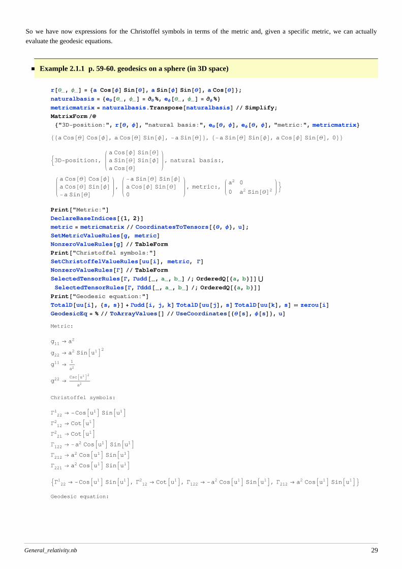
So we have now expressions for the Christoffel symbols in terms of the metric and, given a specific metric, we can actually

evaluate the geodesic equations.General_relativity.nb 28

So we have now expressions for the Christoffel symbols in terms of the metric and, given a specific metric, we can actually

evaluate the geodesic equations.

Example 2.1.1 p. 59-60. geodesics on a sphere (in 3D space)

r@Θ_, Φ_D = 8a Cos@ΦD Sin@ΘD, a Sin@ΦD Sin@ΘD, a Cos@ΘD<;naturalbasis = 8eΘ@Θ_, Φ_D = ¶Θ %, eΦ@Θ_, Φ_D = ¶Φ %<metricmatrix = naturalbasis.Transpose@naturalbasisD Simplify;

MatrixForm 8"3D-position:", r@Θ, ΦD, "natural basis:", eΘ@Θ, ΦD, eΦ@Θ, ΦD, "metric:", metricmatrix<88a Cos@ΘD Cos@ΦD, a Cos@ΘD Sin@ΦD, -a Sin@ΘD<, 8-a Sin@ΘD Sin@ΦD, a Cos@ΦD Sin@ΘD, 0<<:3D-position:,

a Cos@ΦD Sin@ΘDa Sin@ΘD Sin@ΦDa Cos@ΘD , natural basis:,

a Cos@ΘD Cos@ΦDa Cos@ΘD Sin@ΦD-a Sin@ΘD ,

-a Sin@ΘD Sin@ΦDa Cos@ΦD Sin@ΘD0

, metric:,a2 0

0 a2 Sin@ΘD2>

Print@"Metric:"DDeclareBaseIndices@81, 2<Dmetric = metricmatrix CoordinatesToTensors@8Θ, Φ<, uD;SetMetricValueRules@g, metricDNonzeroValueRules@gD TableForm

Print@"Christoffel symbols:"DSetChristoffelValueRules@uu@iD, metric, GDNonzeroValueRules@GD TableForm

SelectedTensorRules@G, Gudd@_, a_, b_D ; OrderedQ@8a, b<DD ÜSelectedTensorRules@G, Gddd@_, a_, b_D ; OrderedQ@8a, b<DD

Print@"Geodesic equation:"DTotalD@uu@iD, 8s, s<D + Gudd@i, j, kD TotalD@uu@jD, sD TotalD@uu@kD, sD zerou@iDGeodesicEq = % ToArrayValues@D UseCoordinates@8Θ@sD, Φ@sD<, uDMetric:

g11 ® a2

g22 ® a2 SinAu1E2

g11 ®1

a2

g22 ®CscAu1E2

a2

Christoffel symbols:

G 221 ® -CosAu1E SinAu1E

G 122 ® CotAu1E

G 212 ® CotAu1E

G122 ® -a2 CosAu1E SinAu1EG212 ® a2 CosAu1E SinAu1EG221 ® a2 CosAu1E SinAu1E9G 22

1 ® -CosAu1E SinAu1E, G 122 ® CotAu1E, G122 ® -a2 CosAu1E SinAu1E, G212 ® a2 CosAu1E SinAu1E=

Geodesic equation:


â2ui

âsâs+ G jk

iâu

j

âs

âuk

âs zeroi

9-Cos@Θ@sDD Sin@Θ@sDD Φ¢@sD2 + Θ¢¢@sD 0, 2 Cot@Θ@sDD Θ¢@sD Φ¢@sD + Φ¢¢@sD 0=Try to solve the geodesic equation with initial conditions analytically and numerically.

eqs = GeodesicEq Ü 8Θ@0D 1, Θ'@0D 1, Φ@0D 1, Φ'@0D 1<;DSolve@eqs, 8Θ@sD, Φ@sD<, sDNDSolve@eqs, 8Θ@sD, Φ@sD<, 8s, 0, 2 Π<Dr@Θ@sD, Φ@sDD . %@@1DD . a ® 1;

ParametricPlot3D@%, 8s, 0, Π<, ViewPoint ® 8-1, 1, 1 <, ImageSize ® 88 ´ 72, 3 ´ 72<D;DSolveA9Θ@0D 1, Φ@0D 1, Θ¢@0D 1, Φ¢@0D 1,

-Cos@Θ@sDD Sin@Θ@sDD Φ¢@sD2 + Θ¢¢@sD 0, 2 Cot@Θ@sDD Θ¢@sD Φ¢@sD + Φ¢¢@sD 0=, 8Θ@sD, Φ@sD<, sE88Θ@sD ® InterpolatingFunction@880., 6.28319<<, <>D@sD,

Φ@sD ® InterpolatingFunction@880., 6.28319<<, <>D@sD<<

-0.5

-0.250

0.25

-1-0.5

00.5

1

-0.5

0

0.5

-0.5

-0.250

0.25

-1-0.5

00.5

1

ø Plot of the numerically found geodesic. ø

For circles of latitude the geodesic equation is satisfied only by the equator.

Block@8Θ, Φ, Θ0, a<,H* circles of latitude *LΘ@s_D := Θ0; Φ@s_D := s Ha Sin@Θ0DL;Print@GeodesicEq, ", ", 8Θ@sD, Θ'@sD, Φ@sD, Φ'@sD< . s ® 0D;Θ0 = Π 2;

Print@GeodesicEq, ", ", 8Θ@sD, Θ'@sD, Φ@sD, Φ'@sD< . s ® 0D;D:-

Cot@Θ0Da2

0, True>, :Θ0, 0, 0,Csc@Θ0D

a>

8True, True<, : Π

2, 0, 0,

1

a>

Example 2.1.2 p. 61-63. geodesic equation for the Robertson-Walker spacetime

DeclareBaseIndices@80, 1, 2, 3<DVar = 8t, r, Θ, Φ<;cmetric = DiagonalMatrixB:1, -R@tD2

1

1 - k r2, -R@tD2 r2, -R@tD2 r2 Sin@ΘD2>F;


cmetric = DiagonalMatrixB:1, -R@tD2

1 - k r2, -R@tD2 r2, -R@tD2 r2 Sin@ΘD2>F;

% MatrixForm

Dt@sD2 [email protected]@VarD, -R@tD2E TraditionalForm

1 0 0 0

0 -R@tD21-k r2

0 0

0 0 -r2 R@tD2 0

0 0 0 -r2 R@tD2 Sin@ΘD2

Hâ sL2 Hâ tL2 - RHtL2Hâ rL2

1 - k r2+ r2 Hâ ΘL2 + r2 Hâ ΦL2 sin2HΘL

BeginTime = SessionTime@D;metric = cmetric CoordinatesToTensors@VarDSetMetricValues@g, metricDSetChristoffelValueRules@xu@iD, metric, G, Simplify@ð, Trig ® FalseD &DSelectedTensorRules@G, Gudd@a_, b_, c_D ; OrderedQ@8b, c<DD

UseCoordinates@VarD TableForm

Print@"Geodesic equation for the Robertson-Walker spacetime"DTotalD@xu@iD, 8u, u<D + Gudd@i, j, kD TotalD@xu@jD, uD TotalD@xu@kD, uD zerou@iD% ToArrayValues@D UseCoordinates@VarD;Collect@ð, R@tD R'@tDD & %;

CollectAð, r Ik r2 - 1ME & %;

% TableForm TraditionalForm

Print@"Compare with eqn@2, 20D, p.62."DPrint@"- - - - Time used: ", N@SessionTime@D - BeginTime, 3D, " s"D:81, 0, 0, 0<, :0, -

RAx0E2

1 - k Ix1M2, 0, 0>, :0, 0, -RAx0E2 Ix1M2

, 0>, :0, 0, 0, -RAx0E2SinAx2E2 Ix1M2>>

G 110 ®

R@tD R¢@tD1-k r2

G 220 ® r2 R@tD R¢@tD

G 330 ® r2 R@tD Sin@ΘD2 R¢@tD

G 011 ®

R¢@tDR@tD

G 111 ®

k r

1-k r2

G 221 ® r I-1 + k r2M

G 331 ® r I-1 + k r2M Sin@ΘD2

G 022 ®

R¢@tDR@tD

G 122 ®

1

r

G 332 ® -Cos@ΘD Sin@ΘD

G 033 ®

R¢@tDR@tD

G 133 ®

1

r

G 233 ® Cot@ΘD

Geodesic equation for the Robertson-Walker spacetime

â2xi

âuâu+ G jk

iâx

j

âu

âxk

âu zeroi


â2t

âu2+ RHtL K âr

âuO2

1-k r2+ r2 J âΘ

âuN2

+ r2 J âΦ

âuN2

sin2HΘL R¢HtL 0

k r K âr

âuO2

1-k r2+

2ât

âuR¢ HtL âr

âu

RHtL +â2r

âu2+ r Ik r2 - 1M J âΘ

âuN2

+ J âΦ

âuN2

sin2HΘL 0

-cosHΘL sinHΘL J âΦ

âuN2

+2

âr

âu

âΘ

âu

r+

â2Θ

âu2+

2ât

âu

âΘ

âuR¢ HtL

RHtL 0

2âr

âu

âΦ

âu

r+ 2 cotHΘL âΘ

âu

âΦ

âu+

2ât

âuR¢ HtL âΦ

âu

RHtL +â2Φ

âu2 0


- - - - Time used: 10.4 s

More examples: geodesics on special surfaces (in 3D space).

msg = "trumpet H'mbuti, vuvuzelaL";Reduce@8Ρ > 0, Π 2 < Θ < Π, Abs@zD Ρ Tan@Θ - Π 2D,

z -1 Ρ, x Ρ Cos@ΦD, y Ρ Sin@ΦD<, 8Ρ, x, y, z<, RealsDr@Φ_, Θ_D = 8%@@3, 2DD, %@@4, 2DD, %@@5, 2DD< . Θ ® HΘ + ΠL 2;

Π

2< Θ < Π && Ρ -Tan@ΘD && x Cos@ΦD -Tan@ΘD && y Sin@ΦD -Tan@ΘD && z -

1

-Tan@ΘDmsg = "sphere";

r@Φ_, Θ_D = 8Cos@ΦD Sin@ΘD, Sin@ΦD Sin@ΘD, Cos@ΘD<;msg = "cardio potatoid";

pΦ@Φ_D = -H-Π - ΦL2 H1 3 + 3 ΦL H1 2 - ΦL HΠ - ΦL2 550;

pΘ@Θ_D = Θ2 H2 - ΘL HΠ - ΘL2 4;

r@Φ_, Θ_D = H1 + pΦ@ΦD pΘ@ΘDL 8Cos@ΦD Sin@ΘD, Sin@ΦD Sin@ΘD, Cos@ΘD<;Print@msgDPrint@"3D-position:"Dr@Φ, ΘD MatrixForm Short

naturalbasis = 8eΦ, eΘ< = 8¶Φr@Φ, ΘD, ¶Θr@Φ, ΘD<;Print@"natural basis:"DMatrixForm 8eΦ, eΘ< Short

Print@"metric:"Dmetricmatrix = naturalbasis.Transpose@naturalbasisDH*Simplify*L;% Short MatrixForm

Potatoid = ParametricPlot3D@r@Φ, ΘD, 8Φ, -Π, Π<,8Θ, 0 + 2 $MachineEpsilon, Π<, PlotPoints -> 840, 40<, DisplayFunction ® IdentityDcardio potatoid

3D-position:

J1 -H2-ΘL 6

2200N Cos@ΦD Sin@ΘD

1H1L 1

natural basis:

: H1L Cos@ΦD Sin@ΘD - 1

1 + 1H1L 1 1

,1 + H1L 1 Sin@ΘD1

1

>metric:

99H1L2 Cos@ΘD2 + H1L2 + H1 - 1L2, 1=, 1=


Graphics3D

DeclareBaseIndices@81, 2<Dmetric = metricmatrix CoordinatesToTensors@8Φ, Θ<, uD;Block@8SetMetricValueRules<,SetMetricValueRules@g_, MT_, flavor_: IdentityD :=

Module@8i, j<,SetTensorValueRules@Tensor@g, 8Void, Void<, 8i, j<D ToFlavor@flavorD, MTD;SetTensorValueRules@Tensor@g, 8i, j<, 8Void, Void<D ToFlavor@flavorD,Identity@Inverse@MTDDDD;

SetMetricValueRules@g, metricD; SetChristoffelValueRules@uu@iD, metric, GD;DPrint@"g:"D;NonzeroValueRules@gD Shallow TableForm

Print@"G:"D;SelectedTensorRules@G, Gudd@_, a_, b_D ;

OrderedQ@8a, b<DD Shallow TableForm

Print@"Geodesic equation:"DTotalD@uu@iD, 8s, s<D + Gudd@i, j, kD TotalD@uu@jD, sD TotalD@uu@kD,

sD zerou@iDGeodesicEq = % ToArrayValues@D UseCoordinates@8Φ@sD, Θ@sD<, uD;GeodesicEq Short

eqs := GeodesicEq Ü IBConds;

g:

83 ® Plus@3D, 3 ® Plus@3D, 3 ® Plus@3D, 3 ® Plus@3D,3 ® Times@2D, 3 ® Times@2D, 3 ® Times@2D, 3 ® Times@2D<

G:

83 ® Times@2D, 3 ® Times@2D, 3 ® Times@2D,3 ® Times@2D, 3 ® Times@2D, 3 ® Times@2D<

Geodesic equation:

â2ui

âsâs+ G jk

iâu

j

âs

âuk

âs zeroi

81 0, 1 0<A collection of geodetics starting at the same point on the chosen surface:

Ι = .4; sRange = 8s, 0, Ι 2 Π <;geodplots = 8<; Clear@funs, IBvecsDDs = .001; Μ = 250; Α = 1;8Φ0, Θ0< = 8 Π 4, Π 3<;nmax = 9;

Do@HΒ = Hn - 1L 2 Π nmax;

IBConds = 8Θ@0D Θ0, Θ'@0D Α Cos@ΒD, Φ@0D Φ0, Φ'@0D Α Sin@ΒD<;solrule = NDSolve@eqs, 8Φ, Θ<, sRangeD;8Φsol, Θsol< = 8solrule@@1, 1, 2DD, solrule@@1, 2, 2DD<;geodesic@s_D := r@Φsol@sD, Θsol@sDD;funs@nD = 8Φsol, Θsol, geodesic<;AppendTo @geodplots, ParametricPlot3D@

1.001 geodesic@sD + 80, 0, .01<, Evaluate@sRangeD, DisplayFunction ® IdentityDD;r0 = r@Φsol@0D, Θsol@0DD;rs = r@Φsol@0D + Φsol '@0D Ds, Θsol@0D + Θsol '@0D DsD;Dr = rs - r0;

IBvecs@nD = 8


IBvecs@nD = 8Graphics3D@8Hue@0D, [email protected]<, Point@r@Φsol@0DD, Θsol@0DDD,Graphics3D@[email protected], Line@8r0, r0 + Μ Dr<D<D,Graphics3D@[email protected], [email protected], Point@r0 + Μ DrD<D<;

AppendTo@geodplots, IBvecs@nDD;L,8n, 1, nmax<D H* End of Do *LvP = 5 r@Φ0, Θ0D;Show@8

Graphics3D@EdgeForm@DD, Potatoid,

geodplots, Graphics3D@[email protected], Point@80, 0, 0<D<D<,Axes ® True, AxesLabel ® 8"X", "Y", "Z"<,DisplayFunction ® $DisplayFunction, ViewPoint ® vP, ImageSize ® 72 ´ 6D;

-1

-0.5

0

0.5

1

X

-1

0

1

Y

-1

0

1

Z

-1

-0.5

0

0.5

1

X

ø Plot of the chosen surface with a collection of geodetics starting at the same point. ø

Export@"C:\\USERS\\LUMA\\Mathematica\\_Tensorrechnung\\2.1- Geodesics_on_special_surfaces.dxf", %, "DXF"D

C:\USERS\LUMA\Mathematica\_Tensorrechnung\2.1 - Geodesics_on_special_surfaces.dxf

More details on a selected geodetics:

nselect = 3;8Φsol, Θsol, geodesic< = funs@nselectD;pl0 = ParametricPlot3D@geodesic@sD, Evaluate@sRangeD,

AxesLabel ® 8"X", "Y", "Z"<, ViewPoint ® vP, DisplayFunction ® IdentityD;pl1 = Plot@8Θsol@sD, Φsol@sD<, Evaluate@sRangeD, PlotRange ® 880, sRange@@3DD<, Automatic<,

AxesLabel ® 8"s", "Θ, Φ"<, PlotStyle ® 8Hue@0D, [email protected]<, DisplayFunction ® IdentityD;pl2 = Plot@8Θsol '@sD, Φsol '@sD<, Evaluate@sRangeD,

PlotRange ® 880, sRange@@3DD<, Automatic<, AxesLabel ® 8"s", "Θ', Φ'"<,PlotStyle ® 8Hue@0D, [email protected]<, DisplayFunction ® IdentityD;


PlotStyle ® 8Hue@0D, [email protected]<, DisplayFunction ® IdentityD;pl3 = PlotB

8Norm@geodesic'@sDD, -Norm@8Θsol '@sD, Φsol '@sD<D<, Evaluate@sRangeD,PlotRange ® 880, sRange@@3DD<, All<, AxesLabel ® :"s", "Ègeodesic'@sDÈ, -ÈHΘ'@sD

Φ'@sDLÈ">,PlotStyle ® 8Hue@0D, [email protected]<, DisplayFunction ® IdentityF;

pl4 = ParametricPlot@8Θsol@sD, Φsol@sD<, Evaluate@sRangeD, AxesLabel ® 8"Θ", "Φ"<,PlotStyle ® [email protected]<, DisplayFunction ® IdentityD;

Show@pl0, IBvecs@nselectD, DisplayFunction ® $DisplayFunction, ImageSize ® 72 ´ 4D;Show@GraphicsArray@88pl1, pl3<, 8pl2, pl4<<D, ImageSize ® 72 ´ 6D;

-1

-0.5

0

0.5

X

0.50.75

11.25

1.5Y

0.40.50.6

Z

-1

-0.5

0

0.5

X

0.40.50.6

Z

0.5 1 1.5 2 2.5s

0.2

0.4

0.6

0.8

1Θ', Φ'

1.05 1.15 1.2 1.25 1.3Θ

1.5

2

2.5

Φ

0.5 1 1.5 2 2.5s

0.8

1.2

1.4

1.6

1.8

2

2.2

Θ, Φ

0.5 1 1.5 2 2.5s

-1

-0.5

0.5

1

Ègeodesic'@sDÈ, -ÈHΘ'@sDΦ'@sDLÈ

ø Details on a selected geodetic. ø

"Geodesics are locally extremes of length. [...] Feynman has a cute illustration in a book of this. Suppose you want to arrive back

where you are now in one hour of local time, but with a maximum of time having elapsed for you. Note that going uphill takes

you to a place where, informally speaking, time goes faster. But moving fast causes time to go "slower" (informally speaking).

What is the tradeoff between the two which leads to an optimum of wasted time? Geodesics in space-time are the *free-fall*

paths of objects. So the right thing to do is to shoot yourself out of a cannon so that in free fall, you return to the same spot on the

ground." (Keith Ramsay)


2.2 Parallel vectors along a curve p. 64 - 71


DeclareBaseIndices@81, 2, 3, 4<Dlabs = 8x, ∆, g, G<;DefineTensorShortcuts@88x, e, Λ, Λ0, zero<, 1<,88∆, g<, 2<,88G<, 3<DDeclareZeroTensor@zeroDDeclareTensorSymmetries@G, 3, 81, 82, 3<<DH* A simple routine for formatted output of tensors: *LST@tensor_D :=

Print@"Tensor ", EinsteinArray@D@tensorD, " is ", ToArrayValues@D@tensorDD;H* A victor is a graphical rappresentation of a vector as a pin. pin-

head Hgreen=STARTL bloody pin-tip Hred=STOPL: *Lvictor@a_, b_, linecolor_: [email protected] := 8

Graphics3D@[email protected], [email protected], Point@aD<D,Graphics3D@8linecolor, Line@8a, a + b<D<D,Graphics3D@[email protected], [email protected], Point@a + bD<D<;H* nbProjHvL are the components of a vector v in the basis 8eΘ, eΦ, eΘeΦ<: *L

nbProj@v_D := 8"v=", v MatrixForm, "nbProjHvL=",8v.eΘ@Θ, ΦD, v.eΦ@Θ, ΦD, v.eΘ@Θ, ΦDeΦ@Θ, ΦD< MatrixForm< Simplify;

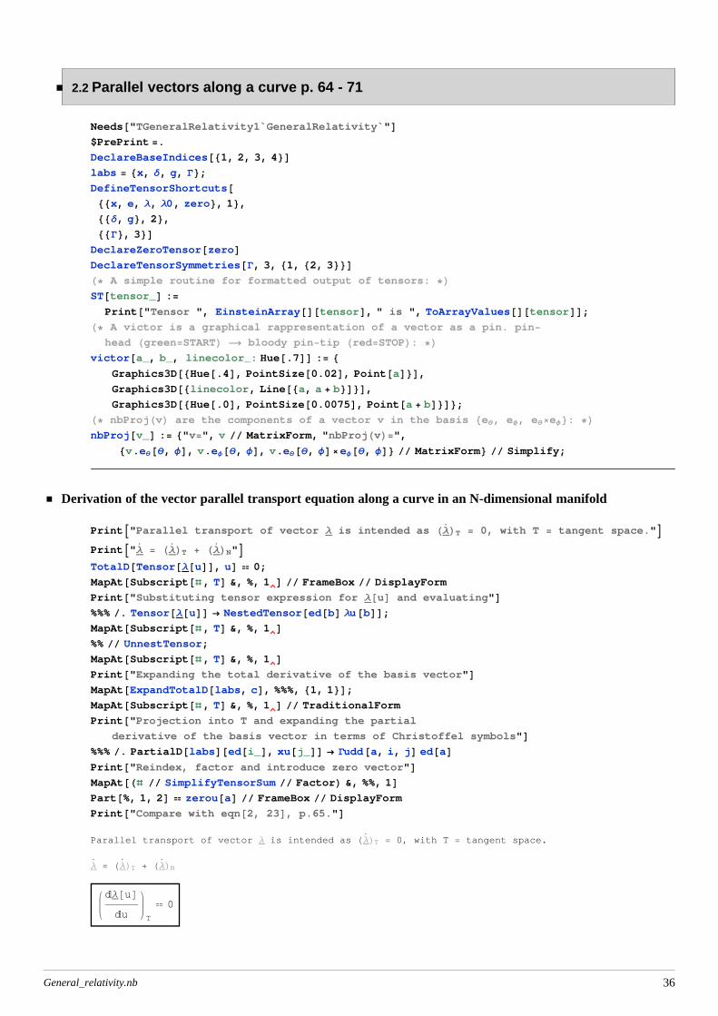
Derivation of the vector parallel transport equation along a curve in an N-dimensional manifold

PrintA"Parallel transport of vector Λ is intended as HΛ LT = 0, with T = tangent space."E

PrintA"Λ

= HΛ LT + HΛ

LN"ETotalD@Tensor@Λ@uDD, uD 0;

MapAt@Subscript@ð, TD &, %, 1 D FrameBox DisplayForm

Print@"Substituting tensor expression for Λ@uD and evaluating"D%%% . Tensor@Λ@uDD ® NestedTensor@ed@bD Λu@bDD;MapAt@Subscript@ð, TD &, %, 1 D%% UnnestTensor;

MapAt@Subscript@ð, TD &, %, 1 DPrint@"Expanding the total derivative of the basis vector"DMapAt@ExpandTotalD@labs, cD, %%%, 81, 1<D;MapAt@Subscript@ð, TD &, %, 1 D TraditionalForm

Print@"Projection into T and expanding the partial

derivative of the basis vector in terms of Christoffel symbols"D%%% . PartialD@labsD@ed@i_D, xu@j_DD ® Gudd@a, i, jD ed@aDPrint@"Reindex, factor and introduce zero vector"DMapAt@Hð SimplifyTensorSum FactorL &, %%, 1DPart@%, 1, 2D zerou@aD FrameBox DisplayForm

Print@"Compare with eqn@2, 23D, p.65."DParallel transport of vector Λ is intended as HΛ

LT = 0, with T = tangent space.

Λ

= HΛ LT + HΛ

LN

âΛ@uDâu T

0


Substituting tensor expression for Λ@uD and evaluating

âIeb ΛbMâu

T

0

Λbâeb

âu+ eb

âΛb

âuT

0

Expanding the total derivative of the basis vector

eb

âΛb

âu+ Λb

âxc

âu

¶eb

¶ xcT

0

Projection into T and expanding the partial

derivative of the basis vector in terms of Christoffel symbols

ea G bca Λb

âxc

âu+ eb

âΛb

âu 0

Reindex, factor and introduce zero vector

ea G bca Λb

âxc

âu+

âΛa

âu 0

G bca Λb

âxc

âu+

âΛa

âu zeroa


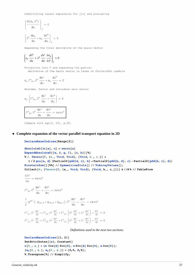
Complete expansion of the vector parallel transport equation in 2D

DeclareBaseIndices@Range@2DDAbsoluteD@Λu@aD, uD zerou@aDExpandAbsoluteD@8x, ∆, g, G<, 8c, b<D@%D% . Tensor@G, 8a_, Void, Void<, 8Void, b_, c_<D ®

1 2 guu@a, dD HPartialD@gdd@d, cD, bD + PartialD@gdd@b, dD, cD - PartialD@gdd@b, cD, dDLEinsteinSum@D@%%D SymmetrizeSlots@D ToArrayValues@D;Collect@ð, 8Tensor@G, 8a_, Void, Void<, 8Void, b_, c_<D<D & % TableForm

DΛa

du zeroa

G cba Λb

âxc

âu+

âΛa

âu zeroa

1

2gad I-gcb,d + gcd,b + gdb,cM Λb

âxc

âu+

âΛa

âu zeroa

G 111 Λ1 âx1

âu+ G 22

1 Λ2 âx2

âu+ G 12

1 KΛ2 âx1

âu+ Λ1 âx2

âuO +

âΛ1

âu 0

G 112 Λ1 âx1

âu+ G 22

2 Λ2 âx2

âu+ G 12

2 KΛ2 âx1

âu+ Λ1 âx2

âuO +

âΛ2

âu 0

Definitions used in the next two sections:

DeclareBaseIndices@81, 2<DSetAttributes@8a<, ConstantDr@Θ_, Φ_D = 8a Cos@ΦD Sin@ΘD, a Sin@ΦD Sin@ΘD, a Cos@ΘD<;8eΘ@Θ_, Φ_D, eΦ@Θ_, Φ_D< = 8¶Θ %, ¶Φ %<;%.Transpose@%D Simplify;


%.Transpose@%D Simplify;

metric = % CoordinatesToTensors@8Θ, Φ<, xD;SetMetricValueRules@g, metricDSetChristoffelValueRules@xu@iD, metric, GD

Example 2.2.1 p. 66-68. vector parallel transport on a 2D-sphere

SetAttributes@8Θ0, Ω, Α<, ConstantDPrint@"Vector parallel transport equation on a sphere with radius a"Deqns = TotalD@Λu@mD, tD + Gudd@m, n, sD Λu@nD TotalD@xu@sD, tD zerou@mD% ToArrayValues@D TableForm

Print@"...and along a circle of latitude Θ0 for vector Λ@tD with I.C. on Λ@0D"DSetTensorValueRules@xu@iD, 8Θ0, t<Dxu@iD ST

eqns = Heqns ToArrayValues@DL . Λu@i_D ® Λu@iD@tD;conds = 8Λu@1D@0D Cos@ΑD a, Λu@2D@0D Sin@ΑD Ha Sin@Θ0DL<;eqns Ü conds TableForm FrameBox DisplayForm

sols = DSolve@eqns Ü conds, 8Λu@1D, Λu@2D<, tDP1T . Cos@Θ0D ® Ω;

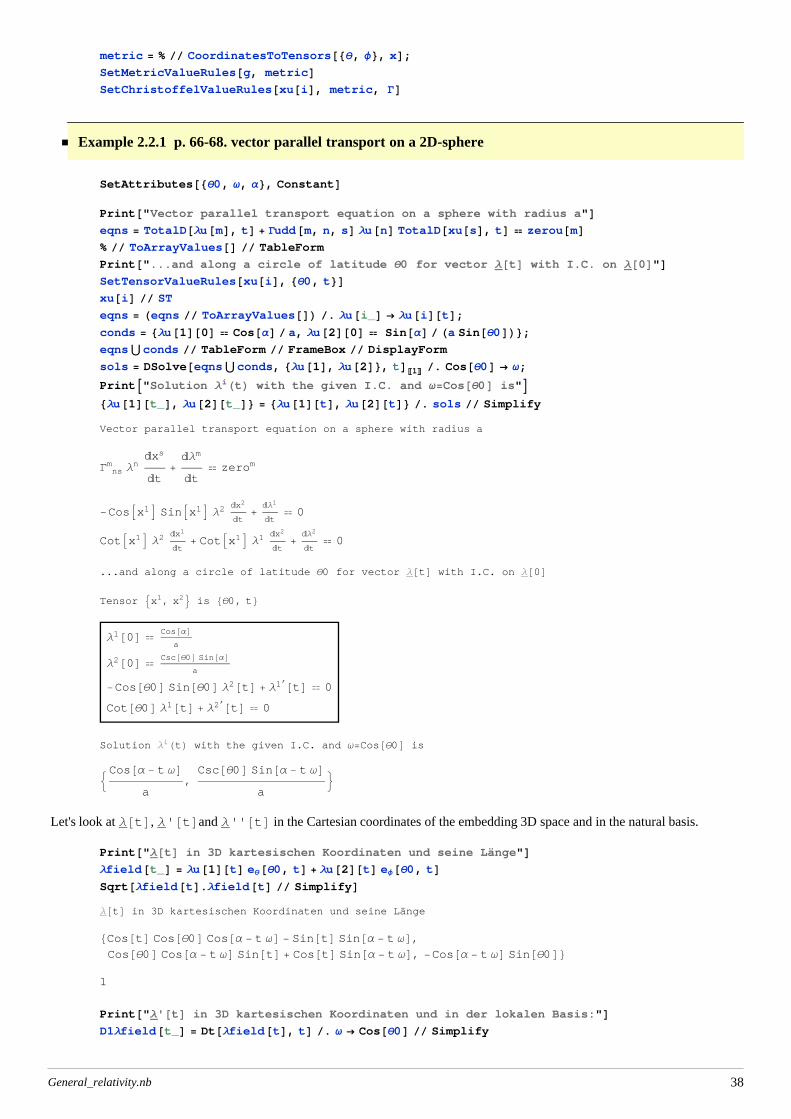
PrintA"Solution ΛiHtL with the given I.C. and Ω=Cos@Θ0D is"E8Λu@1D@t_D, Λu@2D@t_D< = 8Λu@1D@tD, Λu@2D@tD< . sols Simplify

Vector parallel transport equation on a sphere with radius a

G nsm Λn

âxs

ât+

âΛm

ât zerom

-CosAx1E SinAx1E Λ2 âx2

ât+

âΛ1

ât 0

CotAx1E Λ2 âx1

ât+ CotAx1E Λ1 âx2

ât+

âΛ2

ât 0

...and along a circle of latitude Θ0 for vector Λ@tD with I.C. on Λ@0DTensor 9x1, x2= is 8Θ0, t<

Λ1@0D Cos@ΑD

a

Λ2@0D Csc@Θ0D Sin@ΑD

a

-Cos@Θ0D Sin@Θ0D Λ2@tD + Λ1¢@tD 0

Cot@Θ0D Λ1@tD + Λ2¢@tD 0

Solution ΛiHtL with the given I.C. and Ω=Cos@Θ0D is

:Cos@Α - t ΩDa

,Csc@Θ0D Sin@Α - t ΩD

a>

Let's look at Λ@tD, Λ'@tDand Λ''@tD in the Cartesian coordinates of the embedding 3D space and in the natural basis.

Print@"Λ@tD in 3D kartesischen Koordinaten und seine Länge"DΛfield@t_D = Λu@1D@tD eΘ@Θ0, tD + Λu@2D@tD eΦ@Θ0, tDSqrt@Λfield@tD.Λfield@tD SimplifyDΛ@tD in 3D kartesischen Koordinaten und seine Länge

8Cos@tD Cos@Θ0D Cos@Α - t ΩD - Sin@tD Sin@Α - t ΩD,Cos@Θ0D Cos@Α - t ΩD Sin@tD + Cos@tD Sin@Α - t ΩD, -Cos@Α - t ΩD Sin@Θ0D<

1

Print@"Λ'@tD in 3D kartesischen Koordinaten und in der lokalen Basis:"DD1Λfield@t_D = Dt@Λfield@tD, tD . Ω ® Cos@Θ0D Simplify


D1Λfield@t_D = Dt@Λfield@tD, tD . Ω ® Cos@Θ0D Simplify8D1Λ[email protected]Θ@Θ0, tD, D1Λ[email protected]Φ@Θ0, tD,D1Λ[email protected]Θ@Θ0, tDeΦ@Θ0, tD< Simplify

Λ'@tD in 3D kartesischen Koordinaten und in der lokalen Basis:

9-Cos@tD Sin@Θ0D2 Sin@Α - t Cos@Θ0DD,-Sin@tD Sin@Θ0D2 Sin@Α - t Cos@Θ0DD, -Cos@Θ0D Sin@Θ0D Sin@Α - t Cos@Θ0DD=

90, 0, -a2 Sin@Θ0D2 Sin@Α - t Cos@Θ0DD=Print@"Λ''@tD in 3D kartesischen Koordinaten und in der lokalen Basis:"DD2Λfield@t_D = Dt@Λfield@tD, 8t, 2<D . Ω ® Cos@Θ0D Simplify8D2Λ[email protected]Θ@Θ0, tD, D2Λ[email protected]Φ@Θ0, tD,

D2Λ[email protected]Θ@Θ0, tDeΦ@Θ0, tD< Simplify

Λ''@tD in 3D kartesischen Koordinaten und in der lokalen Basis:

9Sin@Θ0D2 HCos@tD Cos@Θ0D Cos@Α - t Cos@Θ0DD + Sin@tD Sin@Α - t Cos@Θ0DDL,Sin@Θ0D2 HCos@Θ0D Cos@Α - t Cos@Θ0DD Sin@tD - Cos@tD Sin@Α - t Cos@Θ0DDL,Cos@Θ0D2 Cos@Α - t Cos@Θ0DD Sin@Θ0D=

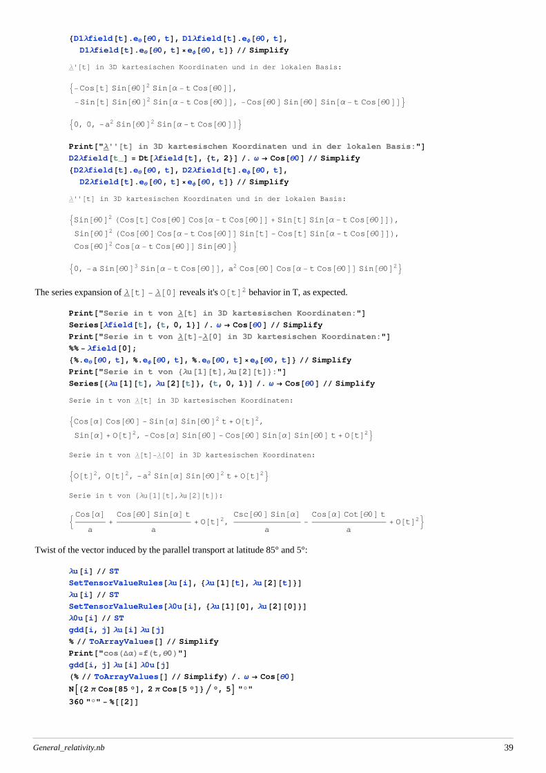
90, -a Sin@Θ0D3 Sin@Α - t Cos@Θ0DD, a2 Cos@Θ0D Cos@Α - t Cos@Θ0DD Sin@Θ0D2=The series expansion of Λ@tD - Λ@0D reveals it's O@tD2 behavior in T, as expected.

Print@"Serie in t von Λ@tD in 3D kartesischen Koordinaten:"DSeries@Λfield@tD, 8t, 0, 1<D . Ω ® Cos@Θ0D Simplify

Print@"Serie in t von Λ@tD-Λ@0D in 3D kartesischen Koordinaten:"D%% - Λfield@0D;8%.eΘ@Θ0, tD, %.eΦ@Θ0, tD, %.eΘ@Θ0, tDeΦ@Θ0, tD< Simplify

Print@"Serie in t von 8Λu@1D@tD,Λu@2D@tD<:"DSeries@8Λu@1D@tD, Λu@2D@tD<, 8t, 0, 1<D . Ω ® Cos@Θ0D Simplify

Serie in t von Λ@tD in 3D kartesischen Koordinaten:

9Cos@ΑD Cos@Θ0D - Sin@ΑD Sin@Θ0D2 t + O@tD2,

Sin@ΑD + O@tD2, -Cos@ΑD Sin@Θ0D - Cos@Θ0D Sin@ΑD Sin@Θ0D t + O@tD2=Serie in t von Λ@tD-Λ@0D in 3D kartesischen Koordinaten:

9O@tD2, O@tD2, -a2 Sin@ΑD Sin@Θ0D2 t + O@tD2=Serie in t von 8Λu@1D@tD,Λu@2D@tD<::Cos@ΑD

a+Cos@Θ0D Sin@ΑD t

a+ O@tD2,

Csc@Θ0D Sin@ΑDa

-Cos@ΑD Cot@Θ0D t

a+ O@tD2>

Twist of the vector induced by the parallel transport at latitude 85° and 5°:

Λu@iD ST

SetTensorValueRules@Λu@iD, 8Λu@1D@tD, Λu@2D@tD<DΛu@iD ST

SetTensorValueRules@Λ0u@iD, 8Λu@1D@0D, Λu@2D@0D<DΛ0u@iD ST

gdd@i, jD Λu@iD Λu@jD% ToArrayValues@D Simplify

Print@"cosHDΑL=fHt,Θ0L"Dgdd@i, jD Λu@iD Λ0u@jDH% ToArrayValues@D SimplifyL . Ω ® Cos@Θ0DNA82 Π Cos@85 °D, 2 Π Cos@5 °D< °, 5E "°"

360 "°" - %@@2DD


Tensor 9Λ1, Λ2= is 9Λ1, Λ2=Tensor 9Λ1, Λ2= is :Cos@Α - t ΩD

a,Csc@Θ0D Sin@Α - t ΩD

a>

Tensor 9Λ01, Λ02= is :Cos@ΑDa

,Csc@Θ0D Sin@ΑD

a>

gij Λi Λj

1

cosHDΑL=fHt,Θ0Lgij Λi Λ0

j

Cos@t Cos@Θ0DD831.376 °, 358.63 °<1.37 °

A graphic representation of the vector parallel transport on a sphere.

BlockA8Α = .4, Θ0 = Π 3, Ω = Cos@Θ0D, a = 1.<,range = 8t, 0, 2 Π, 2 Π 5<;ParametricPlotA8Λu@1D@tD, Λu@2D@tD<, Evaluate@Most@rangeDD,AxesLabel ® 9"Λ1", "Λ2"=, AspectRatio ® Automatic, ImageSize ® 72 ´ 3E;

ΛfieldPlot = Table@victor@r@Θ0, tD, Λfield@tDD, Evaluate@rangeDD;D1ΛfieldPlot = Table@victor@r@Θ0, tD, D1Λfield@tD, [email protected], Evaluate@rangeDD;D2ΛfieldPlot = Table@victor@r@Θ0, tD, D2Λfield@tD, [email protected], Evaluate@rangeDD;naturalbasisPlot = Table@8

victor@r@Θ0, tD, eΘ@Θ0, tD, [email protected], victor@r@Θ0, tD, eΦ@Θ0, tD, [email protected]<,Evaluate@rangeDD; sphereaxisPlot = Graphics3D@[email protected], Line@a 881, 0, 0<, 8-1, 0, 0<<D,Line@a 880, 1, 0<, 80, -1, 0<<D, Line@a 880, 0, 1<, 80, 0, -1<<D<D;

Show@sphereaxisPlot, naturalbasisPlot,

ΛfieldPlot, D1ΛfieldPlot, D2ΛfieldPlot,

Axes ® True, AxesLabel ® 8"X", "Y", "Z"<,PlotRange ® 1.6 88-1, 1<, 8-1, 1<, 8-1, 1<<, ImageSize ® 72 ´ 5D;E

-0.5 0.5 1Λ1

-1

-0.75

-0.5

-0.25

0.25

Λ2


-1

0

1X

-1

0

1Y

-1

0

1

Z

-1

0

1X

-1

0

1Y

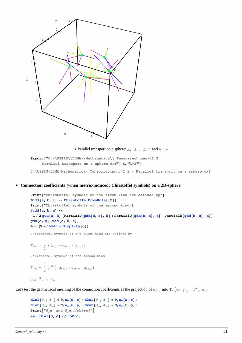
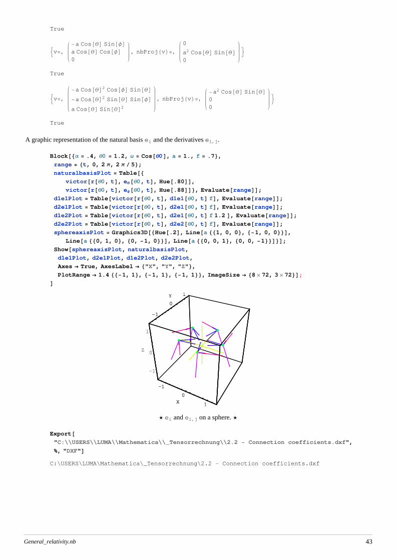
ø Parallel transport on a sphere: Λ, Λ', Λ'' and ei.ø

Export@"C:\\USERS\\LUMA\\Mathematica\\_Tensorrechnung\\2.2- Parallel transport on a sphere.dxf", %, "DXF"D

C:\USERS\LUMA\Mathematica\_Tensorrechnung\2.2 - Parallel transport on a sphere.dxf

Connection coefficients (when metric-induced: Christoffel symbols) on a 2D-sphere

Print@"Christoffel symbols of the first kind are defined by"DGddd@a, b, cD == ChristoffelDownRule@@2DDPrint@"Christoffel symbols of the second kind"DGudd@a, b, cD ==

1 2 guu@a, dD HPartialD@gdd@d, cD, bD + PartialD@gdd@b, dD, cD - PartialD@gdd@b, cD, dDLgdd@a, dD Gudd@d, b, cD;% H% MetricSimplify@gDLChristoffel symbols of the first kind are defined by

Gabc 1


Christoffel symbols of the second kind

G bca

1

2gad I-gbc,d + gbd,c + gdc,bM

gad G bcd Gabc

Let's test the geometrical meaning of the connection coefficients as the projection of ei,j into T: Iei,jMT

= G ijk ek .

d1e1@Θ_, Φ_D = ¶ΘeΘ@Θ, ΦD; d2e1@Θ_, Φ_D = ¶ΦeΘ@Θ, ΦD;d1e2@Θ_, Φ_D = ¶ΘeΦ@Θ, ΦD; d2e2@Θ_, Φ_D = ¶ΦeΦ@Θ, ΦD;PrintA"¶jei and ¶jeinbProj"Eaa = d1e1@Θ, ΦD nbProj


aa = d1e1@Θ, ΦD nbProj

bb = d2e1@Θ, ΦD nbProj

cc = d1e2@Θ, ΦD nbProj

dd = d2e2@Θ, ΦD nbProj

bb == cc

¶jei and ¶jeinbProj

:v=,-a Cos@ΦD Sin@ΘD-a Sin@ΘD Sin@ΦD-a Cos@ΘD , nbProjHvL=,

00

-a3 Sin@ΘD >

:v=,-a Cos@ΘD Sin@ΦDa Cos@ΘD Cos@ΦD0

, nbProjHvL=,

0

a2 Cos@ΘD Sin@ΘD0

>


, nbProjHvL=,

0

a2 Cos@ΘD Sin@ΘD0

>

:v=,-a Cos@ΦD Sin@ΘD-a Sin@ΘD Sin@ΦD0

, nbProjHvL=,

-a2 Cos@ΘD Sin@ΘD0

-a3 Sin@ΘD3

>True

Print@"G"DDrop@NonzeroValueRules@GD UseCoordinates@8Θ, Φ<, uD, -3D8G@1, 1, 1D = 0, G@1, 1, 2D = 0, G@1, 2, 1D = G@1, 1, 2D, G@1, 2, 2D = -Cos@ΘD Sin@ΘD,

G@2, 1, 1D = 0, G@2, 1, 2D = Cot@ΘD, G@2, 2, 1D = G@2, 1, 2D, G@2, 2, 2D = 0< TableForm HoldForm

PrintA"Gkijek and Gk

ijeknbProj"EG@1, 1, 1D eΘ@Θ, ΦD + G@2, 1, 1D eΦ@Θ, ΦD nbProj

Most@ð @@4, 1DDD & Haa %LG@1, 1, 2D eΘ@Θ, ΦD + G@2, 1, 2D eΦ@Θ, ΦD nbProj

Most@ð @@4, 1DDD & Hbb %LG@1, 2, 1D eΘ@Θ, ΦD + G@2, 2, 1D eΦ@Θ, ΦD nbProj

Most@ð @@4, 1DDD & Hcc %LG@1, 2, 2D eΘ@Θ, ΦD + G@2, 2, 2D eΦ@Θ, ΦD nbProj

Most@ð @@4, 1DDD & Hdd %LG

9G 221 ® -CosAx1E SinAx1E, G 12

2 ® CotAx1E, G 212 ® CotAx1E=

G@1, 1, 1D = 0G@1, 1, 2D = 0G@1, 2, 1D = G@1, 1, 2DG@1, 2, 2D = -Cos@ΘD Sin@ΘDG@2, 1, 1D = 0G@2, 1, 2D = Cot@ΘDG@2, 2, 1D = G@2, 1, 2DG@2, 2, 2D = 0

Gkijek and Gk

ijeknbProj:v=,

000

, nbProjHvL=,000

>True


, nbProjHvL=,

0

a2 Cos@ΘD Sin@ΘD0

>


True


, nbProjHvL=,

0

a2 Cos@ΘD Sin@ΘD0

>True

:v=,

-a Cos@ΘD2 Cos@ΦD Sin@ΘD-a Cos@ΘD2 Sin@ΘD Sin@ΦDa Cos@ΘD Sin@ΘD2

, nbProjHvL=,-a2 Cos@ΘD Sin@ΘD00

>True

A graphic representation of the natural basis ei and the derivatives ei,j.

Block@8Α = .4, Θ0 = 1.2, Ω = Cos@Θ0D, a = 1., f = .7<,range = 8t, 0, 2 Π, 2 Π 5<;naturalbasisPlot = Table@8

victor@r@Θ0, tD, eΘ@Θ0, tD, [email protected],victor@r@Θ0, tD, eΦ@Θ0, tD, [email protected]<, Evaluate@rangeDD;

d1e1Plot = Table@victor@r@Θ0, tD, d1e1@Θ0, tD fD, Evaluate@rangeDD;d2e1Plot = Table@victor@r@Θ0, tD, d2e1@Θ0, tD fD, Evaluate@rangeDD;d1e2Plot = Table@victor@r@Θ0, tD, d2e1@Θ0, tD f 1.2 D, Evaluate@rangeDD;d2e2Plot = Table@victor@r@Θ0, tD, d2e2@Θ0, tD fD, Evaluate@rangeDD;sphereaxisPlot = Graphics3D@[email protected], Line@a 881, 0, 0<, 8-1, 0, 0<<D,

Line@a 880, 1, 0<, 80, -1, 0<<D, Line@a 880, 0, 1<, 80, 0, -1<<D<D;Show@sphereaxisPlot, naturalbasisPlot,

d1e1Plot, d2e1Plot, d1e2Plot, d2e2Plot,

Axes ® True, AxesLabel ® 8"X", "Y", "Z"<,PlotRange ® 1.4 88-1, 1<, 8-1, 1<, 8-1, 1<<, ImageSize ® 88 ´ 72, 3 ´ 72<D;D

-1

0

1X

-1

0

1Y

-1

0

1

Z

-1

0

1X

-1

0

1Y

ø ei and ei,j on a sphere. ø

Export@"C:\\USERS\\LUMA\\Mathematica\\_Tensorrechnung\\2.2 - Connection coefficients.dxf",

%, "DXF"DC:\USERS\LUMA\Mathematica\_Tensorrechnung\2.2 - Connection coefficients.dxf


2.3 Absolute and covariant differentiation p. 71 - 79


DeclareBaseIndices@81, 2, 3, 4<Dlabs = 8x, ∆, g, G<;DefineTensorShortcuts@88x, Λ, Μ<, 1<,88∆, g, Τ<, 2<,88G<, 3<DSetTensorValues@∆ud@i, jD, IdentityMatrix@NDimDDDeclareTensorSymmetries@G, 3, 81, 82, 3<<DTensorList = 8Tensor@ΦD, Λu@aD, Λd@aD, Τuu@a, bD, Τdd@a, bD, Τud@a, bD, Τdu@a, bD<;

Absolute differentiation

Haa = AbsoluteD@NestedTensor@ð D, uD;aa Haa UnnestTensor ExpandAbsoluteD@labs, 8i, j<DLL & TensorList TableForm

Print@"last expression fully expanded:"DCollect@ð, 8TotalD@Tensor@x, List@_D, List@VoidDD, uD<D & EinsteinSum@D@Last@%%DD SymmetrizeSlots@D

DΦ

du

âΦ

âu

DΛa

du G ij

aΛj âxi

âu+

âΛa

âu

DΛa

du -G ia

jΛj

âxi

âu+

âΛa

âu

DΤab

du JG ij

bΤaj

+ G ija

ΤjbN âxi

âu+

âΤab

âu

DΤab

du J-G ib

jΤaj - G ia

jΤjbN âxi

âu+

âΤab

âu

DΤ ba

du J-G ib

jΤ ja

+ G ija

Τ bj N âxi

âu+

âΤ ba

âu

DΤab

du J-G ia

jΤj

b+ G ij

bΤa

jN âxi

âu+

âΤab

âu

last expression fully expanded:

DΤab

du IG 11

b Τa1 + G 12

b Τa2 + G 13

b Τa3 + G 14

b Τa4 - G 1a

1 Τ1b - G 1a

2 Τ2b - G 1a

3 Τ3b - G 1a

4 Τ4bM âx1

âu+

IG 12b Τa

1 + G 22b Τa

2 + G 23b Τa

3 + G 24b Τa

4 - G 2a1 Τ1

b - G 2a2 Τ2

b - G 2a3 Τ3

b - G 2a4 Τ4

bM âx2

âu+

IG 13b Τa

1 + G 23b Τa

2 + G 33b Τa

3 + G 34b Τa

4 - G 3a1 Τ1

b - G 3a2 Τ2

b - G 3a3 Τ3

b - G 3a4 Τ4

bM âx3

âu+

IG 14b Τa

1 + G 24b Τa

2 + G 34b Τa

3 + G 44b Τa

4 - G 4a1 Τ1

b - G 4a2 Τ2

b - G 4a3 Τ3

b - G 4a4 Τ4

bM âx4

âu+

âΤab

âu

AbsoluteD@Λu@aD, uD;% H% ExpandAbsoluteD@labs, 8i, j<DLMapAt@ExpandTotalD@labs, iD, %, 2DMapAt@Factor, %, 2DPrint@"in FullForm:"D%% FullForm


DΛa

du G ij

aΛj âxi

âu+

âΛa

âu

DΛa

du G ij

aΛj âxi

âu+

âxi

âu¶xi Λa

DΛa

du

âxi

âuJG ij

aΛj

+ ¶xi ΛaNin FullForm:

Equal@AbsoluteD@Tensor@\[Lambda], List@aD, List@VoidDD, uD,Times@TotalD@Tensor@x, List@iD, List@VoidDD, uD,Plus@Times@Tensor@\[CapitalGamma], List@a,Void,VoidD, List@Void,i,jDD, Tensor@

\[Lambda], List@jD, List@VoidDDD, PartialD@List@x, \[Delta], g, \[CapitalGamma]DD@Tensor@\[Lambda], List@aD, List@VoidDD, Tensor@x, List@iD, List@VoidDDDDDD

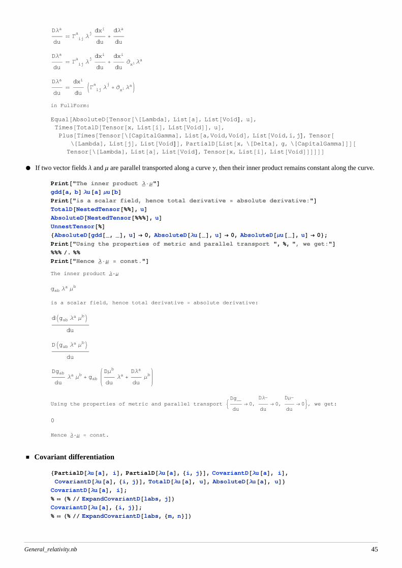
æ If two vector fields Λ and Μ are parallel transported along a curve Γ, then their inner product remains constant along the curve.

Print@"The inner product Λ×Μ"Dgdd@a, bD Λu@aD Μu@bDPrint@"is a scalar field, hence total derivative = absolute derivative:"DTotalD@NestedTensor@%%D, uDAbsoluteD@NestedTensor@%%%D, uDUnnestTensor@%D8AbsoluteD@gdd@_, _D, uD ® 0, AbsoluteD@Λu@_D, uD ® 0, AbsoluteD@Μu@_D, uD ® 0<;Print@"Using the properties of metric and parallel transport ", %, ", we get:"D%%% . %%

Print@"Hence Λ×Μ = const."DThe inner product Λ×Μ

gab Λa Μb

is a scalar field, hence total derivative = absolute derivative:

âIgab Λa ΜbMâu

DIgab Λa ΜbMdu

Dgab

duΛa Μb + gab

DΜb

duΛa +

DΛa

duΜb

Using the properties of metric and parallel transport :Dg__du

® 0,DΛ_

du® 0,

DΜ_

du® 0>, we get:

0

Hence Λ×Μ = const.

Covariant differentiation

8PartialD@Λu@aD, iD, PartialD@Λu@aD, 8i, j<D, CovariantD@Λu@aD, iD,CovariantD@Λu@aD, 8i, j<D, TotalD@Λu@aD, uD, AbsoluteD@Λu@aD, uD<

CovariantD@Λu@aD, iD;% H% ExpandCovariantD@labs, jDLCovariantD@Λu@aD, 8i, j<D;% H% ExpandCovariantD@labs, 8m, n<DL


:Λ ,ia , Λ ,i,j

a, Λ ;i

a , Λ ;i;ja

,âΛa

âu,DΛa

du>

Λ ;ia G ij

aΛj

+ ¶xi Λa

Λ ;i;ja

Λm ¶xj

G ima + ¶

xi,xjΛa - G ji

n IG nma Λm + ¶xn ΛaM + G im

a ¶xj

Λm + G jna JG im

n Λm + ¶xi ΛnNHaa = CovariantD@NestedTensor@ð D, iD;

aa Haa UnnestTensor ExpandCovariantD@labs, 8j<DLL & TensorList TableForm

Print@"last expression fully expanded:"DEinsteinSum@D@Last@%%DDΦ;i Φ,i

Λa;i

G ija

Λj

+ ¶xi Λa

Λa;i -G ia

jΛj + ¶xi Λa

Τab;i

G ijb

Τaj

+ G ija

Τjb

+ ¶xi Τab

Τab;i -G ib

jΤaj - G ia

jΤjb + ¶xi Τab

Τ ba

;i -G ib

jΤ ja

+ G ija

Τ bj

+ ¶xi Τ ba

Τab;i

-G iaj

Τjb

+ G ijb

Τaj

+ ¶xi Τab

last expression fully expanded:

Τab;i

G i1b Τa

1 + G i2b Τa

2 + G i3b Τa

3 + G i4b Τa

4 - G ia1 Τ1

b - G ia2 Τ2

b - G ia3 Τ3

b - G ia4 Τ4

b + ¶xi Τab

æ In general relativity we define the divergence using covariant differentiation.

CovariantD@Λu@aD, aD% ExpandCovariantD@labs, iD% EinsteinSum@D SymmetrizeSlots@D FullSimplifyHaa = CovariantD@NestedTensor@ð D, aD;

aa Haa UnnestTensor ExpandCovariantD@labs, 8i<DLL &

TensorList@@82, 4, 6<DD TableForm

Λ ;aa

G aia Λi + ¶xa Λa

IG 111 + G 12

2 + G 133 + G 14

4 M Λ1 + IG 121 + G 22

2 + G 233 + G 24

4 M Λ2 +

IG 131 + G 23

2 + G 333 + G 34

4 M Λ3 + IG 141 + G 24

2 + G 343 + G 44

4 M Λ4 + ¶x1 Λ1 + ¶x2 Λ2 + ¶x3 Λ3 + ¶x4 Λ4

Λa;a

G aia Λi + ¶xa Λa

Τab;a

G aib Τai + G ai

a Τib + ¶xa Τab

Τ ba

;a -G ab

i Τ ia + G ai

a Τ bi + ¶xa Τ b

a

The divergence of a covariant vector field is defined to be that of the associated contravariant vector field.

Μu@iD guu@i, jD Μd@jDCovariantD@ð, iD & %

% . Tensor@g, 8_, _, Void<, 8Void, Void, Cov@_D<D ® 0

Μi gij

Μj

Μ ;ii g ;i

ijΜj + g

ijΜj;i


Μ ;ii g

ijΜj;i

Example 2.3.1 p. 79. Divergence of a radial field in Euclidean space

H* coordinates *Lcoord = 8r, Θ, Φ<;H* manifold *L 8r Cos@ΦD Sin@ΘD, r Sin@ΦD Sin@ΘD, r Cos@ΘD<;H* natural basis *L Table@¶coord@@nDD %, 8n, 1, Length@coordD<D;H* metric *L%.Transpose@%D Simplify;H* Christoffel symbols in tensor notation *LDeclareBaseIndices@Range@Length@coordDDDSetChristoffelValueRules@xu@iD, CoordinatesToTensors@coord, xD@%%D, GDH* radial field Λ *LSetAttributes@8A, B<, ConstantDSetTensorValueRules@Λu@iD, 8A xu@1D + B, 0, 0<DCovariantD@Λu@iD, iD% ExpandCovariantD@labs, jD% ToArrayValues@D Simplify UseCoordinates@coordD% . A ® 1 . B ® 0

Λ ;ii

G iji

Λj

+ ¶xi Λi

3 A +2 B

r

3

2.4 Geodesic coordinates p. 79 - 81


labs = 8x, ∆, g, G<;DefineTensorShortcuts@88x, x0<, 1<,88g, ∆, X<, 2<,88G, G0, X<, 3<DSetTensorValues@∆ud@a, bD, IdentityMatrix@NDimDDMyRed = StyleForm@Superscript@ð, "¢"D, FontColor ® RGBColor@1, 0, 0DD &;

MyBlue = StyleForm@Superscript@ð, "¢¢"D, FontColor ® RGBColor@0, 0, 1DD &;

DeclareIndexFlavor@8red, MyRed<, 8blue, MyBlue<DDeclareTensorSymmetries@G, 3, 81, 82, 3<<D

1.1) Geodesic coordinates at a point on a sphere

Set up the metric and the Christoffel symbols for a 2D-sphere of radius 1 in spherical coordinates in an embedding Euclidean

space.

ma@u_, v_D = 8Cos@uD Sin@vD, Sin@uD Sin@vD, Cos@vD<;ru = 8u, -Π, Π<; rv = 8v, 0, Π<;H* P0 *L8u0, v0< = 81 3, 1 2<;


H* coordinates *Lco = 8u, v<;H* manifold *Lma@u, vD;H* naturalbasis *L Table@¶co@@nDD %, 8n, 1, Length@coD<D;H* metric *Lg@u_, v_D = %.Transpose@%D Simplify;

DeclareBaseIndices@Range@Length@coDDD;metric = %% CoordinatesToTensors@coD; SetMetricValueRules@g, metricD;H* Christoffel symbols *LSetTensorValueRules@Gudd@a, b, cD, CalculateChristoffelu@xu@iD, metric, SimplifyDDSelectedTensorRules@g, gdd@_, _DD TableForm

SelectedTensorRules@G, Gudd@_, i_, j_D ; OrderedQ@8i, j<DD TableForm

g11 ® SinAx2E2

g22 ® 1

G 121 ® CotAx2E

G 112 ® -

1

2SinA2 x2E

Set the point P0. We need the Christoffel symbols evaluated in P0.

SetTensorValueRules@x0u@iD, 8u0, v0<DHGudd@a, b, cD ToArrayValues@DL . xu@i_D ® x0u@iD . TensorValueRules@x0DSetTensorValueRules@G0udd@a, b, cD, %D:::0, CotB1

2F>, :CotB 1

2F, 0>>, ::-

Sin@1D2

, 0>, 80, 0<>>Calculation of the Jacobian matrix X d

a¢

and the Jacobian determinant in P0.

Print@Xud@reda, dD, " = "D∆ud@a, dD + G0udd@a, d, cD Hxu@cD - x0u@cDL% ToArrayValues@D Simplify;

SetTensorValueRules@Xud@reda, bD, %DSetTensorValueRules@Xud@a, redbD, Inverse@%%D SimplifyDXud@reda, bD ToArrayValues@D UseCoordinates@coD MatrixForm

Print@Xud@reda, dD, " in P0 = "D%% . u ® u0 . v ® v0 MatrixForm

Print@"Jacobian determinant in P0:"DDet@%%DX

da¢

=

Hxc - x0cL G0 dca + ∆ d

a

1 -1

2CotB 1

2F + v CotB 1

2F 1

3H-1 + 3 uL CotB 1

2F

1

6HSin@1D - 3 u Sin@1DL 1

Xd

a¢in P0 =

K 1 00 1

OJacobian determinant in P0:

1

Let's check that the Christoffel symbols in the red coordinates are indeed 0 in P0 .


Print@Xudd@reda, d, eD, " = "DPartialD@labsD@Xud@reda, dD, xu@eDD% ToArrayValues@D;SetTensorValueRules@Xudd@reda, b, cD, %DHGudd@a, b, cD ToFlavor@redDL == Gudd@d, e, fD Xud@reda, dD Xud@e, redbD Xud@f, redcD -

Xud@e, redbD Xud@f, redcD Xudd@reda, e, fDToArrayValues@D %;

% . xu@i_D ® x0u@iD . TensorValueRules@x0DX

dea¢

=

¶xe X da¢

G b¢c¢a¢

-X b¢e X c¢

f X efa¢

+ X b¢e X c¢

f X da¢

G efd

999G 1¢1¢1¢

, G 1¢2¢1¢ =, 9G 2¢1¢

1¢, G 2¢2¢

1¢ ==, 99G 1¢1¢2¢

, G 1¢2¢2¢ =, 9G 2¢1¢

2¢, G 2¢2¢

2¢ === 8880, 0<, 80, 0<<, 880, 0<, 80, 0<<<Calculation of the metric in the red coordinates.

Print@gdd@reda, redbD, " = "DXud@c, redaD Xud@d, redbD gdd@c, dD% ToArrayValues@D Simplify;

SetTensorValues@gdd@reda, redbD, %D%% MatrixForm

ga¢b¢ =

gcd X a¢c X b¢

d

9 JSin@1D2+36 SinAx2E2-6 Sin@1D2 x1+9 Sin@1D2 Ix1M2NK18-9 CotB 1

2F+CotB 1

2F Sin@1D-6 CotB 1

2F Sin@1D x1+9 CotB 1

2F Sin@1D Ix1M2+18 CotB 1

2F x2O2 -

27 CotB 1

2F I-1+3 x1M I2 Cos@1D-2 Cos

K18-9 CotB 1

2F+CotB 1

2F Sin@1D-6 CotB 1

2F Sin@1D 2

-27 CotB 1

2F I-1+3 x1M I2 Cos@1D-2 CosA2 x2E+Sin@1D-2 Sin@1D x2M

K18-9 CotB 1

2F+CotB 1

2F Sin@1D-6 CotB 1

2F Sin@1D x1+9 CotB 1

2F Sin@1D Ix1M2+18 CotB 1

2F x2O2

9 4 CotB 1

2F2 SinAx2E2 I1-3 x1M2+9

K18-9 CotB 1

2F+CotB 1

2F Sin@1D-6 CotB 1

2F Sin@1D x1

2

The metric components are unchanged in P0.

Print@gdd@a, bD, " and ", gdd@reda, redbD, " in P0 ="DToArrayValues@D 8gdd@a, bD, gdd@reda, redbD< . xu@i_D ® x0u@iD .

TensorValueRules@x0D Simplify

MatrixForm % N

%% . List ® Equal

g0red = %%%@@2DD Simplify;

gab and ga¢b¢ in P0 =

:::SinB12

F2

, 0>, 80, 1<>, ::SinB12

F2

, 0>, 80, 1<>>:K 0.229849 0.

0. 1.O, K 0.229849 0.

0. 1.O>

True

Transformation to geodesic coordinates.

Print@xu@redaD, " = "Dxu@aD - x0u@aD + 1 2 G0udd@a, b, cD Hxu@bD - x0u@bDL Hxu@cD - x0u@cDL% ToArrayValues@D FullSimplify;

SetTensorValues@xu@redaD, %D


SetTensorValues@xu@redaD, %Dxu@redaD ToArrayValues@D UseCoordinates@coDSolve@8uu, vv< %, 8u, v<D;Select@%, FreeQ@ð, ComplexD &D;maRed@uu_, vv_D = ma@co . %@@1DD . List ® SequenceD;xa

¢=

xa - x0a +1

2Ixb - x0bM Hxc - x0cL G0 bc

a

:16

H-1 + 3 uL 2 - CotB12

F + 2 v CotB12

F , -1

2+ v -

1

36H1 - 3 uL2 Sin@1D>

1.2) Local Cartesian coordinates at a point on a sphere

8s, j< = JordanDecomposition@g0redD;snor = ð ð.ð & Transpose@sD FullSimplify Transpose;

jscale = FullSimplify@Inverse@Sqrt@Abs@jDDDD;MatrixForm 8"g0red", g0red, "s,j", s, j, "snor,jscale", snor, jscale, Transpose@jscaleD<[email protected] Simplify MatrixForm

:g0red, SinB 1

2F2

0

0 1, s,j, K 0 1

1 0O, 1 0

0 SinB 1

2F2 ,

snor,jscale, K 0 11 0

O, 1 0

0 CscB 1

2F ,

1 0

0 CscB 1

2F >

K 1 00 1

Operm = K 1 0

0 1O;

Pmat = snor.jscale.perm FullSimplify;

transPmat = Transpose@PmatD;invPmat = Inverse@PmatD;MatrixForm 8Pmat, transPmat, invPmat<HtransPmat.g0red.Pmat FullSimplifyL DiagonalMatrix@81, 1<D: 0 CscB 1

2F

1 0,

0 1

CscB 1

2F 0

,0 1

SinB 1

2F 0

>True

SetTensorValues@Xud@reda, bluebD, PmatDPrint@gdd@bluea, bluebD, " in P0 = "Dgdd@redc, reddD Xud@redc, blueaD Xud@redd, bluebDToArrayValues@D@%D . xu@i_D ® x0u@iD . TensorValueRules@x0D Simplify

ga¢¢b¢¢ in P0 =

gc¢d¢ X a¢¢c¢

X b¢¢d¢

881, 0<, 80, 1<<Transformation to local Cartesian coordinates.

Print@xu@blueaD, " = "DinvPmat.ToArrayValues@D@xu@redaDD FullSimplify;

SetTensorValues@xu@blueaD, %Dxu@blueaD ToArrayValues@D UseCoordinates@coD


xu@blueaD ToArrayValues@D UseCoordinates@coDSolve@8uuu, vvv< %, 8u, v<D;Select@%, FreeQ@ð, ComplexD &D;maBlue@uuu_, vvv_D = ma@co . %@@1DD . List ® SequenceD;xa

¢¢=

:-1

2+ v -

1

36H1 - 3 uL2 Sin@1D, 1

6H-1 + 3 uL 2 - CotB 1

2F + 2 v CotB1

2F SinB1

2F>

1.3) Coordinate mesh (spherical, geodesic and local Cartesian) at a point on a sphere

8P0 = ma@u0, v0D, g@u0, v0D MatrixForm<% N

H* coordinates *L coR = 8uu, vv<;H* manifold *L maRed@uu, vvD;H* naturalbasis *L Table@¶coR@@nDD %, 8n, 1, Length@coRD<D;H* metric *L gR@uu_, vv_D = %.Transpose@%D MatrixForm;8P0 == maRed@0, 0D, gR@0, 0D< Simplify

H* coordinates *L coB = 8uuu, vvv<;H* manifold *L maBlue@uuu, vvvD;H* naturalbasis *L Table@¶coB@@nDD %, 8n, 1, Length@coBD<D;H* metric *L gB@uuu_, vvv_D = %.Transpose@%D MatrixForm;8P0 == maBlue@0, 0D, gB@0, 0D< Simplify

::CosB13

F SinB 12

F, SinB13

F SinB 12

F, CosB12

F>, SinB 1

2F2

0

0 1>

:80.453036, 0.156865, 0.877583<, K 0.229849 0.0. 1.

O>:True, SinB 1

2F2

0

0 1>

:True, K 1 00 1

O>H* Graphics data *Ln = 10; Du = .2; Dv = .2;

Table@ParametricPlot3D@ma@u, vnD, 8u, u0 - Du, u0 + Du<, DisplayFunction ® IdentityD,8vn, v0 - Dv, v0 + Dv, 2 Dv Hn - 1L<D;Table@ParametricPlot3D@ma@un, vD, 8v, v0 - Dv, v0 + Dv<, DisplayFunction ® IdentityD,8un, u0 - Du, u0 + Du, 2 Du Hn - 1L<D;CoordinateMesh = 8%, %%<;n = 10; Du = .2; Dv = .2;

Table@ParametricPlot3D@maRed@u, vnD, 8u, -Du, Du<, DisplayFunction ® IdentityD,8vn, -Dv, Dv, 2 Dv Hn - 1L<D;Table@ParametricPlot3D@maRed@un, vD, 8v, -Dv, Dv<, DisplayFunction ® IdentityD,8un, -Du, Du, 2 Du Hn - 1L<D;CoordinateMeshRed = 8%, %%<;n = 10; Du = .2; Dv = .2;

Table@ParametricPlot3D@maBlue@u, vnD, 8u, -Du, Du<, DisplayFunction ® IdentityD,8vn, -Dv, Dv, 2 Dv Hn - 1L<D;Table@ParametricPlot3D@maBlue@un, vD, 8v, -Dv, Dv<, DisplayFunction ® IdentityD,8un, -Du, Du, 2 Du Hn - 1L<D;CoordinateMeshBlue = 8%, %%<;


CoordinateMeshBlue = 8%, %%<;pp = 40;

uvSphere = ParametricPlot3D@ma@u, vD, Evaluate@ruD,Evaluate@rvD, PlotPoints -> 8pp, pp<, DisplayFunction ® IdentityD;

VP = ViewPoint ® 2 P0;

Show@Graphics3D@EdgeForm@D, Axes ® True,

AxesLabel ® 8"X", "Y", "Z"<, VP, ImageSize ® 88 ´ 72, 6 ´ 72<D,Graphics3D@Point@N@P0DDD,CoordinateMesh,

CoordinateMeshRed,

CoordinateMeshBlue,

uvSphereD;

-1

-0.5

0

0.5

1

X

-0.5

0

0.5

1

Y

-1

-0.5

0

0.5

1

Z

-0.5

0

0.5

1

Y

-1

-0.5

0

0.5

1

Z

ø Spherical, geodesic and local Cartesian coordinates together on a sphere in P0. ø

Export@"C:\\USERS\\LUMA\\Mathematica\\_Tensorrechnung\\2.4 - Spherical,

geodesic and local Cartesian coordinates on a sphere.dxf", %, "DXF"DC:\USERS\LUMA\Mathematica\_Tensorrechnung\2.4 -

Spherical, geodesic and local Cartesian coordinates on a sphere.dxf

Show@Graphics3D@EdgeForm@D, Axes ® True,

AxesLabel ® 8"X", "Y", "Z"<, VP, PlotRange ® 880.2, .7<, 8-.1, .42<, 8.7, 1<<D,Graphics3D@Point@P0DD, ð, DisplayFunction ® IdentityD & 8CoordinateMesh, CoordinateMeshRed, CoordinateMeshBlue<;

Show@GraphicsArray@%D, ImageSize ® 72 ´ 8D;


0.2

0.3

0.4

0.5

0.6

X

00.2

0.4

Y

0.70.8

0.91

Z

00.2

0.4

Y

0.70.8

0.91

Z

0.2

0.3

0.4

0.5

0.6

X

00.2

0.4

Y

0.70.8

0.91

Z

00.2

0.4

Y

0.70.8

0.91

Z

0.2

0.3

0.4

0.5

0.6

X

00.2

0.4

Y

0.70.8

0.91

Z

00.2

0.4

Y

0.70.8

0.91

Z

ø Spherical, geodesic and local Cartesian coordinates on a sphere in P0. ø

2) Local Cartesian coordinates in the Painlevé-Gullstrand metric (a generalized Schwarzschild metric withoff-diagonal terms)

g0red =

1

3-

2

30 0

-2

3-1 0 0

0 0 -9 M2 0

0 0 0 -9 M2

; asmpt = M > 0;

8s, j< = JordanDecomposition@g0redD;invs = Inverse@sD FullSimplify;

snor = ð ð.ð & Transpose@sD FullSimplify Transpose;

invsnor = Inverse@snorD FullSimplify;

jscale = FullSimplify@Inverse@Sqrt@Abs@jDDD, asmptD;perm =

0 1 0 01 0 0 00 0 0 10 0 1 0

;

1) Since the metric matrix is symmetrical a Jordan decomposition will give a diagonal matrix.

MatrixForm 8s, invs, j, s.j.invs< Simplify8Hs.j.invs SimplifyL g0red, Hinvs.g0red.s SimplifyL j<

:-2+ 10

6

-2+ 10

6

0 0

1 1 0 00 0 0 10 0 1 0

,

3

5

2

1

2+

1

10

0 0

-

3

5

2

1

2-

1

10

0 0

0 0 0 10 0 1 0

,

1

3J-1 - 10 N 0 0 0

01

3J-1 + 10 N 0 0

0 0 -9 M2 0

0 0 0 -9 M2

,

1

3-

2

30 0

-2

3-1 0 0

0 0 -9 M2 0

0 0 0 -9 M2

>

8True, True<We calculate a new, orthogonal similarity matrix by normalizing the columns.


MatrixForm 8invsnor, invsnor.snor FullSimplify<invsnor == [email protected] FullSimplifyL g0red, Hinvsnor.g0red.snor FullSimplifyL j<

:1

2-

1

10

1

2+

1

10

0 0

-1

2+

1

10

1

2-

1

10

0 0

0 0 0 10 0 1 0

,

1 0 0 00 1 0 00 0 1 00 0 0 1

>

True

8True, True<2) Scaling matrix...

MatrixForm 8jscale, Inverse@jscaleD<jscale == [email protected] Simplify MatrixForm

:

1

3J-1 + 10 N 0 0 0

01

3J1 + 10 N 0 0

0 01

3 M0

0 0 01

3 M

,

3

-1+ 10

0 0 0

03

1+ 10

0 0

0 0 3 M 00 0 0 3 M

>

True

-1 0 0 00 1 0 00 0 -1 00 0 0 -1

3) Permutation...

perm.Hjscale.j.jscaleL Simplify MatrixForm

%.perm Simplify MatrixForm

perm == Transpose@permD0 1 0 0-1 0 0 00 0 0 -10 0 -1 0

1 0 0 00 -1 0 00 0 -1 00 0 0 -1

True

4) The FN P matrix is then...


Hperm.jscale.invsnorL.g0red.Hsnor.jscale.permL FullSimplify MatrixForm

Pmat = snor.jscale.perm FullSimplify;

transPmat = Transpose@PmatD FullSimplify;

invPmat = Inverse@PmatD FullSimplify ToRadicals;

MatrixForm 8Pmat, transPmat, invPmat<Print@"Have we transPmat.g0red.Pmat==Η ?"DHtransPmat.g0red.Pmat FullSimplifyL DiagonalMatrix@81, -1, -1, -1<D1 0 0 00 -1 0 00 0 -1 00 0 0 -1

:-

1

2+

2

5-

1

2+

2

50 0

1

30J-5 + 4 10 N 1

30J5 + 4 10 N 0 0

0 01

3 M0

0 0 01

3 M

,

-1

2+

2

5

1

30J-5 + 4 10 N 0 0

-1

2+

2

5

1

30J5 + 4 10 N 0 0

0 01

3 M0

0 0 01

3 M

,

-1

6+

22

5

3-

1

2+

2

50 0

1

30J-5 + 4 10 N 1

2+

2

50 0

0 0 3 M 00 0 0 3 M

>

Have we transPmat.g0red.Pmat==Η ?

True

FN: "The implication of this for general relativity is that about each point of spacetime we can introduce a coordinate system in

which GΝΣΜ

» 0, gΜΝ » ΗΜΝ [...] showing that locally the spacetime of general relativity looks like that of special relativity."

2.5 The spacetime of general relativity p. 82 - 85


labs = 8x, ∆, g, G<;DefineTensorShortcuts@88x, j, p, dx, f, u, zero<, 1<,88∆, g, Η, zero, F<, 2<,88G, zero<, 3<DDeclareZeroTensor@zeroDFlatToCurvedSpacetime = 8Η ® g, TotalD ® AbsoluteD, Dif ® Cov<;

Proper time dΤ for a particle and equation of motion under a force f :

Print@"Flat spacetime:"D; 9dΤ2 Ηdd@Μ, ΝD dxu@ΜD dxu@ΝD, TotalD@pu@ΜD, ΤD fu@ΜD=Print@"Curved spacetime:"D; H% . FlatToCurvedSpacetimeL


Flat spacetime:

:dΤ2 dxΜdxΝ ΗΜΝ,

âpΜ

âΤ f

Μ>Curved spacetime:

:dΤ2 dxΜdxΝ gΜΝ,

DpΜ

dΤ f

Μ>Maxwell equations in curved spacetime:

Heqn@2, 67D = 8PartialD@Fuu@Μ, ΝD, ΝD Μ0 ju@ΜD,Fold@ð1 + HPartialD@Fdd@ð1, ð2D, ð3D & ð2L &,

0, Table@RotateLeft@8Μ, Ν, Σ<, iD, 8i, 0, 2<DD zeroddd@Μ, Ν, ΣD<LHeqn@2, 68D = eqn@2, 67D . FlatToCurvedSpacetimeL9F ,Ν

ΜΝ Μ0 j

Μ, FΜΝ,Σ + FΝΣ,Μ + FΣΜ,Ν zeroΜΝΣ=

9F ;ΝΜΝ

Μ0 jΜ, FΜΝ;Σ + FΝΣ;Μ + FΣΜ;Ν zeroΜΝΣ=

Definition of time/light/space-like vectors.

MapThread@8ð1, ð2@gdd@Μ, ΝD Λu@ΜD Λu@ΝD, 0D< &,88"vector Λ timelike", "vector Λ null HlightlikeL", "vector Λ spacelike"<,8Greater, Equal, Less<<D TableForm FrameBox DisplayForm

vector Λ timelike gΜΝ Λu@ΜD Λu@ΝD > 0

vector Λ null HlightlikeL gΜΝ Λu@ΜD Λu@ΝD 0

vector Λ spacelike gΜΝ Λu@ΜD Λu@ΝD < 0

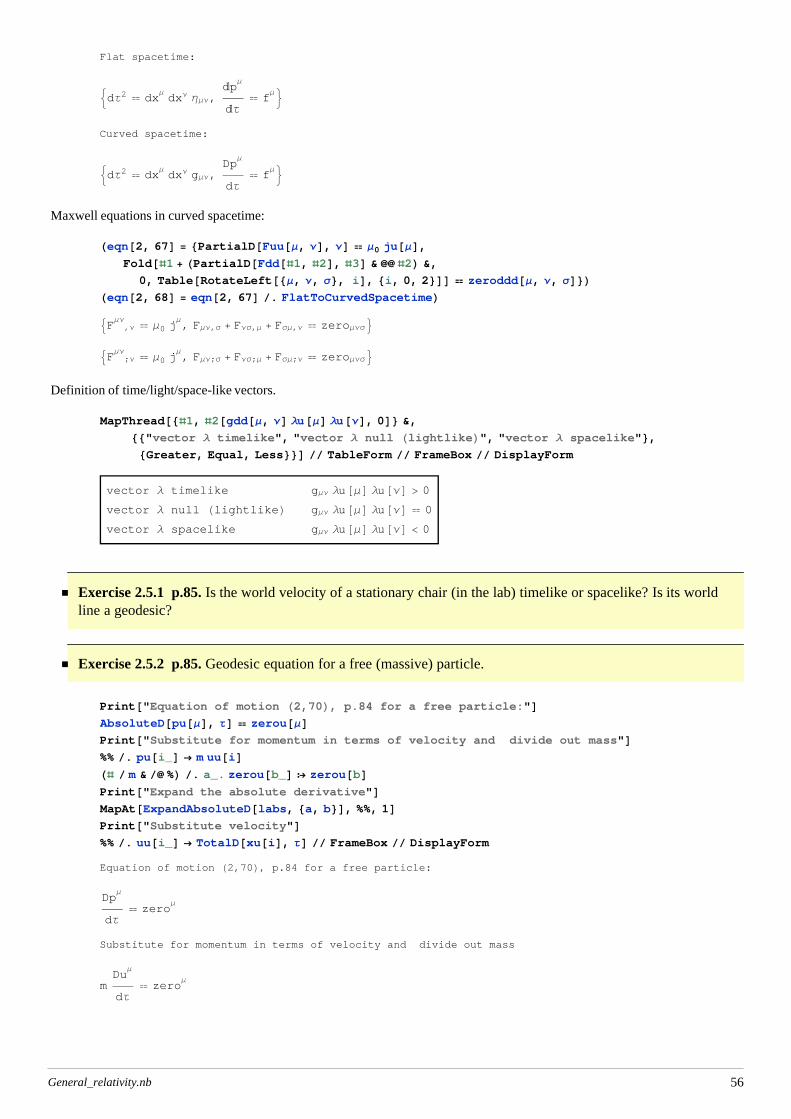
Exercise 2.5.1 p.85. Is the world velocity of a stationary chair (in the lab) timelike or spacelike? Is its world line a geodesic?

Exercise 2.5.2 p.85. Geodesic equation for a free (massive) particle.

Print@"Equation of motion H2,70L, p.84 for a free particle:"DAbsoluteD@pu@ΜD, ΤD zerou@ΜDPrint@"Substitute for momentum in terms of velocity and divide out mass"D%% . pu@i_D ® m uu@iDHð m & %L . a_. zerou@b_D ¦ zerou@bDPrint@"Expand the absolute derivative"DMapAt@ExpandAbsoluteD@labs, 8a, b<D, %%, 1DPrint@"Substitute velocity"D%% . uu@i_D ® TotalD@xu@iD, ΤD FrameBox DisplayForm

Equation of motion H2,70L, p.84 for a free particle:

DpΜ

dΤ zero

Μ

Substitute for momentum in terms of velocity and divide out mass

mDu

Μ

dΤ zero

Μ


DuΜ

dΤ zero

Μ

Expand the absolute derivative

âuΜ

âΤ+ ub G ab

Μâxa

âΤ zero

Μ

Substitute velocity

G abΜ

âxa

âΤ

âxb

âΤ+

â2xΜ

âΤâΤ zero

Μ

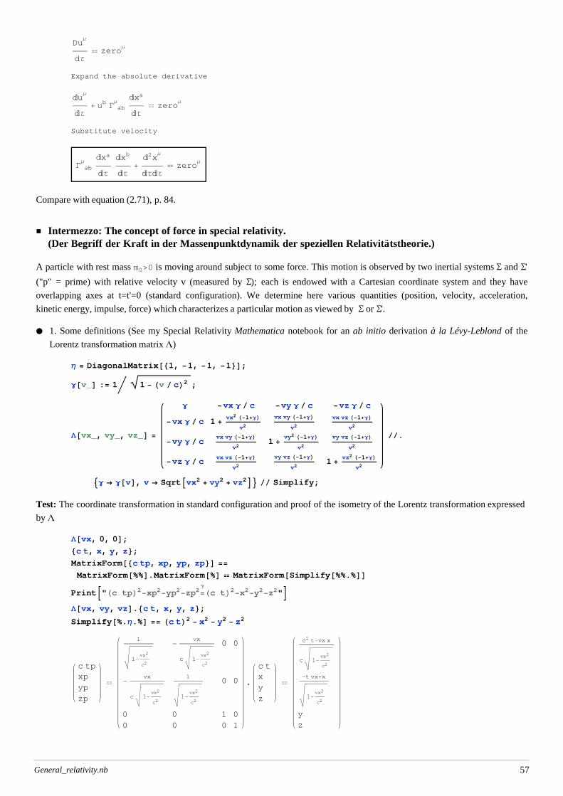
Compare with equation (2.71), p. 84.

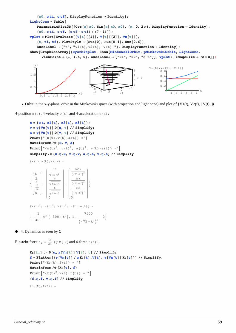
Intermezzo: The concept of force in special relativity.(Der Begriff der Kraft in der Massenpunktdynamik der speziellen Relativitätstheorie.)

A particle with rest mass m0>0 is moving around subject to some force. This motion is observed by two inertial systems S and S'

("p" = prime) with relative velocity v (measured by S); each is endowed with a Cartesian coordinate system and they have

overlapping axes at t=t'=0 (standard configuration). We determine here various quantities (position, velocity, acceleration,

kinetic energy, impulse, force) which characterizes a particular motion as viewed by S or S'.

æ 1. Some definitions (See my Special Relativity Mathematica notebook for an ab initio derivation à la Lévy-Leblond of the

Lorentz transformation matrix L.)

Η = DiagonalMatrix@81, -1, -1, -1<D;Γ@v_D := 1 1 - Hv cL2 ;

L@vx_, vy_, vz_D =

Γ -vx Γ c -vy Γ c -vz Γ c

-vx Γ c 1 +vx2 H-1+ΓL

v2

vx vy H-1+ΓLv2

vx vz H-1+ΓLv2

-vy Γ cvx vy H-1+ΓL

v21 +

vy2 H-1+ΓLv2

vy vz H-1+ΓLv2

-vz Γ cvx vz H-1+ΓL

v2

vy vz H-1+ΓLv2

1 +vz2 H-1+ΓL

v2

.

9Γ ® Γ@vD, v ® SqrtAvx2 + vy2 + vz2E= Simplify;

Test: The coordinate transformation in standard configuration and proof of the isometry of the Lorentz transformation expressed

by L.

L@vx, 0, 0D;8c t, x, y, z<;MatrixForm@8c tp, xp, yp, zp<D ==

MatrixForm@%%D.MatrixForm@%D MatrixForm@Simplify@%%.%DDPrintB"Hc tpL2-xp2-yp2-zp2=

?Hc tL2-x2-y2-z2"FL@vx, vy, vzD.8c t, x, y, z<;Simplify@%.Η.%D == Hc tL2 - x2 - y2 - z2

c tpxpypzp

1

1-vx2

c2

-vx

c 1-vx2

c2

0 0

-vx

c 1-vx2

c2

1

1-vx2

c2

0 0

0 0 1 00 0 0 1

.

c txyz

c2 t-vx x

c 1-vx2

c2

-t vx+x

1-vx2

c2

yz


Hc tpL2-xp2-yp2-zp2=?Hc tL2-x2-y2-z2

True

æ 2. A little collection of motions restrained to the x-y-plane.

msg = "Kräftefreie Bewegung";

Ν = 1 2;

x1@t_D := Ν t;

x2@t_D := Ν t; x3@t_D := 0

msg = "Hyperbolische Bewegung";

g = 1 4; Α = 3 Π 4;

x1@t_D := Cos@ΑD c2 g 1 + Hg t cL2 - 1 ; x2@t_D := Sin@ΑD c2 g 1 + Hg t cL2 - 1 ;

x3@t_D := 0

msg = "Bewegung auf Lissajous-Orbit";H* Caution: Problems with the inverse t =fHt'L, see below !*Lx1@t_D := Cos@Π tD 4;

x2@t_D := Sin@tD 4; x3@t_D := 0

msg = "Parabolic orbit HBewegung auf Parabel-OrbitL";x1@t_D := t 2;

x2@t_D := t2 20; x3@t_D := 0

For simplicity we assume c=1 and m0>0 ; time t Î [0, 2Π].

c = 1 ; m0 = 1;8ti, tf< = 80, 2 Π<;$Assumptions = 8ti £ t £ tf<;

æ 3. Cinematic as seen by S

Ordinary position X(t), velocity V(t) and acceleration A(t):

Print@" --- ", msg, " --- "DX@t_D := 8x1@tD, x2@tD, x3@tD<V@t_D := D@X@tD, tDVn@t_D := Simplify@Norm@V@tDDDA@t_D := Simplify@D@X@tD, 8t, 2<DDAn@t_D := Simplify@Norm@A@tDDDPrint@"8XHtL, VHtL, AHtL, ÈVHtLÈ, ÈAHtLÈ< ="DMatrixForm 8X@tD, V@tD, A@tD, Vn@tD, An@tD<

--- Parabolic orbit HBewegung auf Parabel-OrbitL ---

8XHtL, VHtL, AHtL, ÈVHtLÈ, ÈAHtLÈ< =

:t

2

t2

20

0

,

1

2t

10

0

,

01

10

0

,25 + t2

10,

1

10>

A graphical representation of the motion.

xyOrbitplot =

ParametricPlot@8x1@x0 cD, x2@x0 cD<, 8x0, c ti, c tf<, AspectRatio ® Automatic,

AxesLabel ® 8"x1", "x2"<, PlotStyle ® 8Hue@0D<, DisplayFunction ® IdentityD;MinkowskiOrbit = ParametricPlot3D@8x1@x0 cD, x2@x0 cD, x0, [email protected]<,8x0, c ti, c tf<, DisplayFunction ® IdentityD;pMinkowskiOrbit = ParametricPlot3D@8x1@x0 cD, x2@x0 cD, 0<,

, D;General_relativity.nb 58

pMinkowskiOrbit = ParametricPlot3D@8x1@x0 cD, x2@x0 cD, 0<,8x0, c ti, c tf<, DisplayFunction ® IdentityD;LightCone = Table@

ParametricPlot3D@8Cos@ΑD x0, Sin@ΑD x0, x0<, 8Α, 0, 2 Π<, DisplayFunction ® IdentityD,8x0, c ti, c tf, Hc tf - c tiL H7 - 1L<D;vplot = Plot@Evaluate@8V@tD@@1DD, V@tD@@2DD, Vn@tD<D,8t, ti, tf<, PlotStyle ® 8Hue@0D, [email protected], [email protected]<,

AxesLabel ® 8"t", "V1HtL,V2HtL,ÈVHtLÈ"<, DisplayFunction ® IdentityD;Show@GraphicsArray@8xyOrbitplot, Show@MinkowskiOrbit, pMinkowskiOrbit, LightCone,

ViewPoint ® 81, 1.4, 0<, AxesLabel ® 8"x1", "x2", "c t"<D, vplot<, ImageSize ® 72 ´ 8DD;

0.5 1 1.5 2 2.5 3x1

0.5

1

1.5

2x2

-505 x1

-5 05x2

0

2

4

6

c t

-505 x1 1 2 3 4 5 6

t

0.2

0.4

0.6

0.8V1HtL,V2HtL,ÈVHtLÈ

ø Orbit in the x-y-plane, orbit in the Minkowski space (with projection and light cone) and plot of V1(t), V2(t), È V(t)È ø

4-position x(t), 4-velocity v(t) and 4-acceleration a(t):

x = 8c t, x1@tD, x2@tD, x3@tD<;v = Γ@Vn@tDD D@x, tD Simplify;

a = Γ@Vn@tDD D@v, tD Simplify;

Print@"8xHtL,vHtL,aHtL< ="DMatrixForm 8x, v, a<PrintA"8xHtL2, vHtL2, aHtL2, vHtL×aHtL< ="ESimplify 8x.Η.x, v.Η.v, a.Η.a, v.Η.a< Simplify

8xHtL,vHtL,aHtL< =

:tt

2

t2

20

0

,

10

75-t2

5

75-t2

t

75-t2

0

,

100 t

I-75+t2M250 t

I-75+t2M2750

I-75+t2M20

>

8xHtL2, vHtL2, aHtL2, vHtL×aHtL< =

:-1

400t2 I-300 + t2M, 1,

7500

I-75 + t2M3, 0>

æ 4. Dynamics as seen by S

Einstein-force KE =d

dtHΓ m0 VLand 4-force f(t):

KE@t_D := D@m0 Γ@Vn@tDD V@tD, tD Simplify

f = Flatten@8Γ@Vn@tDD c [email protected]@tD, Γ@Vn@tDD KE@tD<D Simplify;

Print@"8KEHtL,fHtL< = "DMatrixForm 8KE@tD, f<PrintA"8fHtL2,vHtL×fHtL< = "E8f.Η.f, v.Η.f< Simplify

8KEHtL,fHtL< =


:5 t

I75-t2M3275

I75-t2M320

,

100 t

I-75+t2M250 t

I-75+t2M2750

I-75+t2M20

>

8fHtL2,vHtL×fHtL< =

: 7500

I-75 + t2M3, 0>

4-momentum p(t):

p = m0 v;

Γ@Vn@tDD D@p, tD Simplify;

PrintB"pHtL, Γ p HtL and Γ p HtL=?fHtL"F

MatrixForm 8p, %%, %% f<PrintB"Γ p

HtL and Γ p

HtL=

?\!\HK\_E\LHtL"F

D@Rest@pD, tD Simplify;8MatrixForm@%D, % == KE@tD<pHtL, Γ p

HtL and Γ p HtL=

?fHtL

:10

75-t2

5

75-t2

t

75-t2

0

,

100 t

I-75+t2M250 t

I-75+t2M2750

I-75+t2M20

, True>

Γ p HtL and Γ p

HtL=

?KEHtL

:5 t

I75-t2M3275

I75-t2M320

, True>

Kinetic energy T(t):

PrintB" THtL and T HtL=

?\!\HK\_E\LHtL×VHtL"F

T@t_D := Im0 Γ@Vn@tDD c2 - m0 c2M Simplify8T@tD,

Simplify HD@T@tD, tD [email protected]@tDL<THtL and T

HtL=?KEHtL×VHtL

:-1 +10

75 - t2, True>

æ 5. Comparisons of forces as seen by S and S'.

(Vergleich der Kräfte, die verschiedene Inertialsysteme bezüglich derselben Bewegung eines Massenpunktes beobachten.)

a) First, we choose a particular relative velocity v of S' with respect to S and set up the corresponding Lorentz transformation

matrix.


L = LB12,1

2,1

2F Simplify;

% MatrixForm

2 -1 -1 -1

-14

3

1

3

1

3

-11

3

4

3

1

3

-11

3

1

3

4

3

b) 4-position x'(t') as seen by S'.

Î Warning: In general the inverse t=f(t')to be calculated by the Solve[] statement may cause serious problems!

xp = L.x Simplify;8tip, tfp< = 8xp@@1DD . t ® ti, xp@@1DD . t ® tf<;$Assumptions = 8tip £ tp £ tfp<;Solve@8c tp == xp@@1DD<, tDtrule = %@@1, 1DD; H* soluzione scelta Hchosen solutionL: t=0 per tp=0 *Lxp = xp . trule Simplify;

xp MatrixForm

::t ® 15 - 5 45 - 4 tp >, :t ® 15 + 5 45 - 4 tp >>tp1

6J15 - 5 45 - 4 tp - 2 tpN

1

6J105 - 7 5 45 - 4 tp - 8 tpN

1

3J-15 + 5 45 - 4 tp - tpN

c) Ordinary velocity V'(t')and its norm as seen by S'.

Xp@tp_D = Rest@xpD;Vp@tp_D := Simplify@D@Xp@tpD, tpDDVnp@tp_D := Simplify@Norm@Vp@tpDDDMatrixForm 8Vp@tpD, Vnp@tpD< N Simplify

:-0.333333 +

0.745356

45.-4. tp

-1.33333 +5.21749

45.-4. tp

-0.333333 -1.49071

45.-4. tp

, 1.4142115. - 1.67705 45. - 4. tp - 1. tp

11.25 - 1. tp>

d) 4-velocity v'(t') and 4-acceleration a'(t')as seen by S'.

vp = Γ@Vnp@tpDD D@xp, tpD Simplify;

ap = Γ@Vnp@tpDD D@vp, tpD Simplify;

MatrixForm 8vp, ap<8vp.Η.vp, ap.Η.vp< Simplify


:

45-4 tp

-75+6 5 45-4 tp +4 tp

5 - 45-4 tp

3 -75+6 5 45-4 tp +4 tp

7 5 -4 45-4 tp

3 -75+6 5 45-4 tp +4 tp

-2 5 - 45-4 tp

3 -75+6 5 45-4 tp +4 tp

,

6 K-45 5 +10 45-4 tp +4 5 tpO45-4 tp K-75+6 5 45-4 tp +4 tpO22 K-15+2 5 45-4 tp O

3 K-75+6 5 45-4 tp +4 tpO210 K-3+ 5 45-4 tp O

3 K-75+6 5 45-4 tp +4 tpO210 K-12+ 5 45-4 tp O

3 K-75+6 5 45-4 tp +4 tpO2

>

81, 0<e) Einstein-force KE' Ht'Land 4-force f'(t')as seen by S'.

KsE@tp_D = D@m0 Γ@Vnp@tpDD Vp@tpD, tpD Simplify;

fp@tp_D = Flatten@8Γ@Vnp@tpDD c [email protected]@tpD, Γ@Vnp@tpDD KsE@tpD<D Simplify;

MatrixForm 8KsE@tpD, fp@tpD<vp.Η.fp@tpD Simplify

:

2 K15 K-6 5 + 45-4 tp O+8 5 tpO3 H-45+4 tpL K-75+6 5 45-4 tp +4 tpO32

10 K-45 5 +3 45-4 tp +4 5 tpO3 H-45+4 tpL K-75+6 5 45-4 tp +4 tpO32

10 K-45 5 +12 45-4 tp +4 5 tpO3 H-45+4 tpL K-75+6 5 45-4 tp +4 tpO32

,

60-6 5 45-4 tp

K-75+6 5 45-4 tp +4 tpO2

-2 K15 K-6 5 + 45-4 tp O+8 5 tpO

3 45-4 tp K-75+6 5 45-4 tp +4 tpO2

-10 K-45 5 +3 45-4 tp +4 5 tpO

3 45-4 tp K-75+6 5 45-4 tp +4 tpO2

-10 K-45 5 +12 45-4 tp +4 5 tpO

3 45-4 tp K-75+6 5 45-4 tp +4 tpO2

>

0

f) Is the 4-force f'(t')as seen by S' and calculated directly from the 4-position x'(t') identical to the 4-force calculated with

the Lorentz transformation of the 4-force f(t)as seen by S with t®t'?

L.f . trule Simplify;

% MatrixForm

Simplify@fp@tpD == %%D60-6 5 45-4 tp

K-75+6 5 45-4 tp +4 tpO22 K-15+2 5 45-4 tp O

3 K-75+6 5 45-4 tp +4 tpO210 K-3+ 5 45-4 tp O

3 K-75+6 5 45-4 tp +4 tpO210 K-12+ 5 45-4 tp O

3 K-75+6 5 45-4 tp +4 tpO2

True

Yes, it is! As it should...

"In moving from the flat spacetime of special relativity to the curved spacetime of general

relativity we hope somehow to incorporate the effects of gravity, and the point of view we

are adopting is that gravity is not a force, and that gravitational effects may be explained in

terms of the curvature of spacetime." (FN)


"In moving from the flat spacetime of special relativity to the curved spacetime of general

relativity we hope somehow to incorporate the effects of gravity, and the point of view we

are adopting is that gravity is not a force, and that gravitational effects may be explained in

terms of the curvature of spacetime." (FN)

2.6 Newton's laws of motion p. 86 - 87

2.7 Gravitational potential and the geodesic p. 87 - 89


labs = 8x, ∆, g, G<;DeclareBaseIndices@80, 1, 2, 3<DDefineTensorShortcuts@88x, v<, 1<,88∆, g, Η, h<, 2<,88G, h<, 3<DDeclareTensorSymmetries@G, 3, 81, 82, 3<<D

From the geodesic equation describing the motion of a free massive particle in GR we can recover the Newtonian equation of

motion of a particle moving in a gravitational field by means of a weak&quasi-static field and a slow motion approximation. This

is done here in three "easy" steps... We suppose that gΜΝ = ΗΜΝ + hΜΝ with h << Η = diag(1,-1,-1,-1) (This means also

that the coordinates xΝ are nearly Cartesian).

æ First, from the geodesic equation using the proper time Τ as (affine) parameter we get the geodesic equation using the coordi-

nate time t=t(Τ)as (non-affine) parameter; the inverse is Τ=Τ(t). (See also Exercise 2.1.1, p.63, and subsection 2.1.)

Print@"1L Geodesic equation with the coordinate time as parameter"DAbsoluteD@vu@ΜD, ΤD 0

AbsoluteD@vu@ΜD, tD h@Τ@tDD vu@ΜD% ExpandAbsoluteD@labs, 8Ν, Σ<DHeqn@2, 75D = % . vu@i_D ® TotalD@xu@iD, tDL FrameBox DisplayForm

Print@"Hsee eqn@2,75D and eqn@2,76D, p.87L\nwhere"Dh@Τ@tDD == TotalD@Τ, 8t, t<D TotalD@Τ, tD TraditionalForm

Print@"considering that"DHoldFormAI-f''@ΤD f'@ΤD-2 . Τ ® InverseFunction@fD@tDM

InverseFunction@fD''@tD InverseFunction@fD'@tDEReleaseHold@

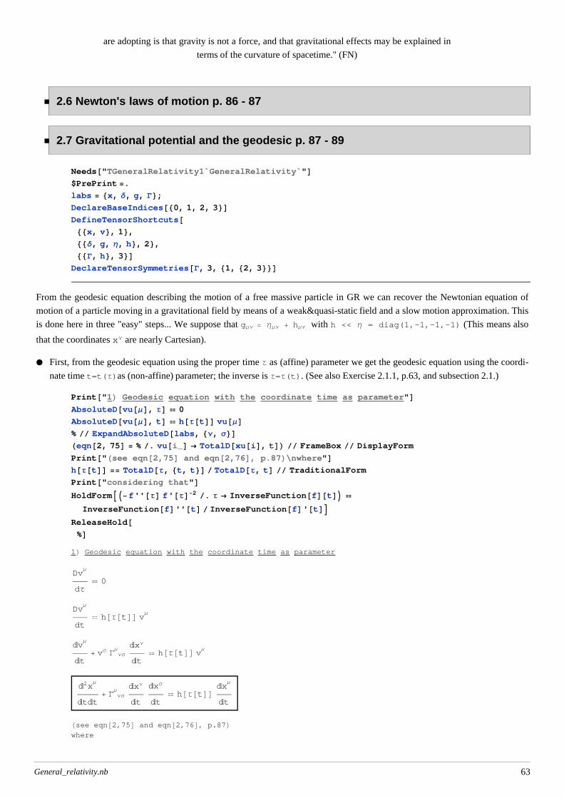
%D1L Geodesic equation with the coordinate time as parameter

DvΜ

dΤ 0

DvΜ

dt h@Τ@tDD v

Μ

âvΜ

ât+ vΣ G ΝΣ

Μ âxΝ

ât h@Τ@tDD v

Μ

â2xΜ

âtât+ G ΝΣ

Μ âxΝ

ât

âxΣ

ât h@Τ@tDD âx

Μ

ât

Hsee eqn@2,75D and eqn@2,76D, p.87Lwhere


hHΤHtLL â2Τ

ât2

âΤ

ât

considering that

-f¢¢@ΤDf¢@ΤD2

. Τ ® fH-1L@tD fH-1L¢¢@tDfH-1L¢@tD

True

Hsee eqn@2,75D and eqn@2,76D, p.87Lwhere

hHΤHtLL â2Τ

ât2

âΤ

ât

considering that

-f¢¢@ΤDf¢@ΤD2

. Τ ® fH-1L@tD fH-1L¢¢@tDfH-1L¢@tD

True

æ Now we construct all the approximations needed.

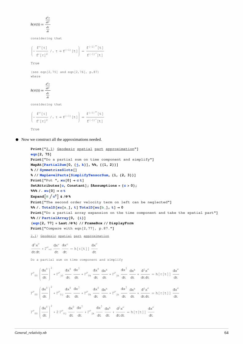
Print@"2,1L Geodesic spatial part approximation"Deqn@2, 75DPrint@"Do a partial sum on time component and simplify"DMapAt@PartialSum@0, 8j, k<D, %%, 881, 2<<D% SymmetrizeSlots@D% MapLevelParts@SimplifyTensorSum, 81, 82, 3<<DPrint@"Put ", xu@0D ® c tDSetAttributes@c, ConstantD; $Assumptions = 8c > 0<;%%% . xu@0D ® c t

ExpandAð c2E & %

Print@"The second order velocity term on left can be neglected"D%% . TotalD@xu@a_D, tD TotalD@xu@b_D, tD ® 0

Print@"Do a partial array expansion on the time component and take the spatial part"D%% PartialArray@0, 8i<DHeqn@2, 77D = Last %L FrameBox DisplayForm

Print@"Compare with eqn@2,77D, p.87."D2,1L Geodesic spatial part approximation

â2xΜ

âtât+ G ΝΣ

Μ âxΝ

ât

âxΣ

ât h@Τ@tDD âx

Μ

ât

Do a partial sum on time component and simplify

G 00Μ

âx0

ât

2

+ G j0Μ

âx0

ât

âxj

ât+ G 0k

Μâx0

ât

âxk

ât+ G jk

Μâx

j

ât

âxk

ât+

â2xΜ

âtât h@Τ@tDD âx

Μ

ât

G 00Μ

âx0

ât

2

+ G 0jΜ

âx0

ât

âxj

ât+ G 0k

Μâx0

ât

âxk

ât+ G jk

Μâx

j

ât

âxk

ât+

â2xΜ

âtât h@Τ@tDD âx

Μ

ât

G 00Μ

âx0

ât

2

+ 2 G 0jΜ

âx0

ât

âxj

ât+ G jk

Μâx

j

ât

âxk

ât+

â2xΜ

âtât h@Τ@tDD âx

Μ

ât


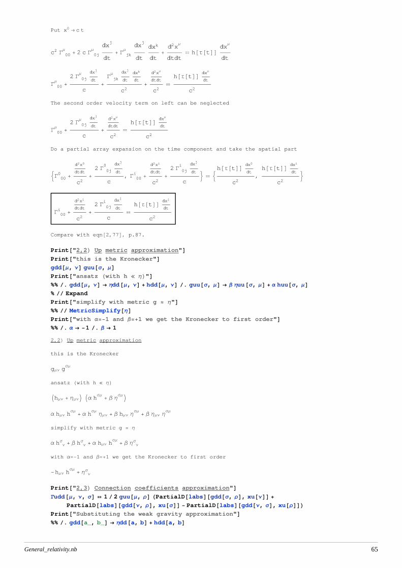
Put x0 ® c t

c2 G 00Μ

+ 2 c G 0jΜ

âxj

ât+ G jk

Μâx

j

ât

âxk

ât+

â2xΜ

âtât h@Τ@tDD âx

Μ

ât

G 00Μ

+2 G 0j

Μ âxj

ât

c+

G jkΜ âxj

ât

âxk

ât

c2+

â2xΜ

âtât

c2

h@Τ@tDD âxΜ

ât

c2

The second order velocity term on left can be neglected

G 00Μ

+2 G 0j

Μ âxj

ât

c+

â2xΜ

âtât

c2

h@Τ@tDD âxΜ

ât

c2

Do a partial array expansion on the time component and take the spatial part

:G 000 +

â2x0

âtât

c2+2 G 0j

0 âxj

ât

c, G 00

i +

â2xi

âtât

c2+2 G 0j

i âxj

ât

c> : h@Τ@tDD âx0

ât

c2,h@Τ@tDD âxi

ât

c2>

G 00i +

â2xi

âtât

c2+2 G 0j

i âxj

ât

c

h@Τ@tDD âxi

ât

c2

Compare with eqn@2,77D, p.87.

Print@"2,2L Up metric approximation"DPrint@"this is the Kronecker"Dgdd@Μ, ΝD guu@Σ, ΜDPrint@"ansatz Hwith h ` ΗL"D%% . gdd@Μ, ΝD ® Ηdd@Μ, ΝD + hdd@Μ, ΝD . guu@Σ, ΜD ® Β Ηuu@Σ, ΜD + Α huu@Σ, ΜD% Expand

Print@"simplify with metric g » Η"D%% MetricSimplify@ΗDPrint@"with Α=-1 and Β=+1 we get the Kronecker to first order"D%% . Α ® -1 . Β ® 1

2,2L Up metric approximation

this is the Kronecker

gΜΝ gΣΜ

ansatz Hwith h ` ΗLIhΜΝ + ΗΜΝM IΑ h

ΣΜ+ Β Η

ΣΜMΑ hΜΝ h

ΣΜ+ Α h

ΣΜΗΜΝ + Β hΜΝ Η

ΣΜ+ Β ΗΜΝ Η

ΣΜ

simplify with metric g » Η

Α h ΝΣ + Β h Ν

Σ + Α hΜΝ hΣΜ

+ Β Η ΝΣ

with Α=-1 and Β=+1 we get the Kronecker to first order

-hΜΝ hΣΜ

+ Η ΝΣ

Print@"2,3L Connection coefficients approximation"DGudd@Μ, Ν, ΣD 1 2 guu@Μ, ΡD HPartialD@labsD@gdd@Σ, ΡD, xu@ΝDD +

PartialD@labsD@gdd@Ν, ΡD, xu@ΣDD - PartialD@labsD@gdd@Ν, ΣD, xu@ΡDDLPrint@"Substituting the weak gravity approximation"D%% . gdd@a_, b_D ® Ηdd@a, bD + hdd@a, bD


%% . gdd@a_, b_D ® Ηdd@a, bD + hdd@a, bDPrint@"Η does not depend on x"D%% NondependentPartialD@8Η, x<DPrint@"Up metric approximation"D%% . guu@a_, b_D ® Ηuu@a, bD - huu@a, bDPrint@"Neglect h compared to Η"D%% . huu@_, _D ® 0

% . PartialD@labsD@hdd@a_, b_D, xu@c_DD ® hddd@a, b, Dif@cDD;GApproxRule = Rule % LHSSymbolsToPatterns@8Μ, Ν, Σ<D;2,3L Connection coefficients approximation

G ΝΣΜ

1

2g

ΜΡ J¶xΣ gΝΡ - ¶xΡ gΝΣ + ¶xΝ gΣΡNSubstituting the weak gravity approximation

G ΝΣΜ

1

2g

ΜΡ J¶xΣ hΝΡ - ¶xΡ hΝΣ + ¶xΝ hΣΡ + ¶xΣ ΗΝΡ - ¶xΡ ΗΝΣ + ¶xΝ ΗΣΡNΗ does not depend on x

G ΝΣΜ

1

2g

ΜΡ J¶xΣ hΝΡ - ¶xΡ hΝΣ + ¶xΝ hΣΡNUp metric approximation

G ΝΣΜ

1

2I-h

ΜΡ+ Η

ΜΡM J¶xΣ hΝΡ - ¶xΡ hΝΣ + ¶xΝ hΣΡNNeglect h compared to Η

G ΝΣΜ

1

2Η

ΜΡ J¶xΣ hΝΡ - ¶xΡ hΝΣ + ¶xΝ hΣΡNPrint@"2,4L Approximation for hHΤHtLL"DPrint@"Start with the derivative of the metric relation"DHTotalD@Τ, tDL2 gdd@Μ, ΝD TotalD@xu@ΜD, tD TotalD@xu@ΝD, tD c2

Print@"Substitute weak gravity metric"D%% . gdd@a_, b_D ® Ηdd@a, bD + hdd@a, bDPrint@"Expand on time coordinate"D%% ExpandAll PartialSum@0, 8i, j<DPrint@"Set ", xu@0D ® c tD;%% . xu@0D ® c t

Print@"Spatial velocities are small compared with time flow"D%% . TotalD@xu@i_D, tD ® 0

Print@"Set ", Ηdd@0, 0D ® 1D%% . Ηdd@0, 0D ® 1

ð & % PowerExpand

Print@"Take the first order Taylor series approximation."DMapAtANormalAð + O@hdd@0, 0DD2E &, %%, 2E TraditionalForm

DΤ = %@@2DD;Print@"Taking the total derivative and expanding"DTotalD@%%%, tDMapAt@ExpandTotalD@labs, aD, %, 2D .PartialD@labsD@hdd@a_, b_D, xu@c_DD ® hddd@a, b, Dif@cDD

Print@"Partial sum on time component and putting ", xu@0D ® c tD%% PartialSum@0, 8i<D% . TotalD@xu@0D, tD ® TotalD@c t, tD TraditionalForm

DDΤ = %@@2DDPrint@"Substitute expressions above"Dh@Τ@tDD TotalD@Τ, 8t, t<D TotalD@Τ, tDh@Τ@tDD DDΤ DΤ


h@Τ@tDD DDΤ DΤ

Print@"Neglect h00 ` Η00 = 1"D%% . hdd@0, 0D ® 0

hApproxRule = Rule %;

2,4L Approximation for hHΤHtLLStart with the derivative of the metric relation

Dt@Τ, tD2 gΜΝ

âxΜ

ât

âxΝ

ât

c2

Substitute weak gravity metric

Dt@Τ, tD2 IhΜΝ + ΗΜΝM âxΜ

ât

âxΝ

ât

c2

Expand on time coordinate

Dt@Τ, tD2

h00 K âx0

âtO2

c2+

Η00 K âx0

âtO2

c2+hi0

âx0

ât

âxi

ât

c2+

Ηi0

âx0

ât

âxi

ât

c2+h0j

âx0

ât

âxj

ât

c2+

Η0j

âx0

ât

âxj

ât

c2+hij

âxi

ât

âxj

ât

c2+

Ηij

âxi

ât

âxj

ât

c2

Set x0 ® c t

Dt@Τ, tD2 h00 + Η00 +hi0

âxi

ât

c+

Ηi0

âxi

ât

c+h0j

âxj

ât

c+

Η0j

âxj

ât

c+hij

âxi

ât

âxj

ât

c2+

Ηij

âxi

ât

âxj

ât

c2

Spatial velocities are small compared with time flow

Dt@Τ, tD2 h00 + Η00

Set Η00 ® 1

Dt@Τ, tD2 1 + h00

Dt@Τ, tD 1 + h00

Take the first order Taylor series approximation.

â Τ

â t

1

2h00 + 1

Taking the total derivative and expanding

Dt@Τ, 8t, 2<D 1

2

âh00

ât

Dt@Τ, 8t, 2<D 1

2h00,a

âxa

ât

Partial sum on time component and putting x0 ® c t

Dt@Τ, 8t, 2<D 1

2h00,0

âx0

ât+1

2h00,i

âxi

ât

â2 Τ

â t2

1

2c h00,0 +

1

2h00,i

âxi

ât


1

2c h00,0 +

1

2h00,i

âxi

ât

Substitute expressions above

h@Τ@tDD Dt@Τ, 8t, 2<D

Dt@Τ, tD

h@Τ@tDD

1

2c h00,0 +

1

2h00,i

âxi

ât

1 +1

2h00

Neglect h00 ` Η00 = 1

h@Τ@tDD 1

2c h00,0 +

1

2h00,i

âxi

ât

(David Park: "I have kept both terms here, departing slightly from FN. The first term is small because of the quasi-static approxi-

mation. The second term is small because of low spatial velocities.")

æ We put here all together!

Print@"3L Finally..."Deqn@2, 77DPrint@"Replace ", Gudd@i, j, kDD%% . GApproxRule

PrintA"Quasi-static field approximation and Ηi0=0"E%% . hddd@_, _, Dif@0DD ® 0 . Ρ ® k

Print@"Neglect approximation for hHΤHtLL"D%% . hApproxRule

%@@1DD 0

Print@"Test particle mass m and rearranging"DMapAð m c2 &, %%, 82<Eeqn@2, 80D = H%@@1, 2DD -%@@1, 1DD - %@@1, 3DDL;% FrameBox DisplayForm

Print@"Compare with eqn@2,80D, p.88."D3L Finally...

G 00i +

â2xi

âtât

c2+2 G 0j

i âxj

ât

c

h@Τ@tDD âxi

ât

c2

Replace G jki

1

2I-h00,Ρ + 2 h0Ρ,0M ΗiΡ +

â2xi

âtât

c2+

J-h0j,Ρ + h0Ρ,j + hjΡ,0N ΗiΡ âxj

ât

c

h@Τ@tDD âxi

ât

c2

Quasi-static field approximation and Ηi0=0

-1

2h00,k Ηik +

â2xi

âtât

c2+

J-h0j,k + h0k,jN Ηikâxj

ât

c

h@Τ@tDD âxi

ât

c2

Neglect approximation for hHΤHtLL

-1

2h00,k Ηik +

â2xi

âtât

c2+


ât

c

âxi

âtK 1

2c h00,0 +

1

2h00,i

âxi

âtO

c2


-1

2h00,k Ηik +

â2xi

âtât

c2+


ât

c 0

Test particle mass m and rearranging

-1

2c2 m h00,k Ηik + m

â2xi

âtât+ c m J-h0j,k + h0k,jN Ηik

âxj

ât 0

mâ2xi

âtât

1

2c2 m h00,k Ηik - c m J-h0j,k + h0k,jN Ηik

âxj

ât


The second rhs term "clearly smacks of rotation" (FN) and is zero in a nonrotating reference system:

eqnnr = Delete@eqn@2, 80D, 82, 2<Dm

â2xi

âtât

1

2c2 m h00,k Ηik

We can derive the rhs term from a gradient of a potential V:

Ieqn@2, 82D = Tensor@VD == 1 2 c2 hdd@0, 0D + constMPartialD@ð, kD & eqn@2, 82DReverse@%D . Equal ® Rule;

Print@"With ", %, " and intoducing the Kronecker delta we get finally"Deqnnr . %%;H% . %@@2, 3DD ® -∆uu@i, kDL FrameBox DisplayForm

Print@"Compare with eqn@2,81D, p.89."DV const +

1

2c2 h00

V,k 1

2c2 h00,k

With1

2c2 h00,k ® V,k and intoducing the Kronecker delta we get finally

mâ2xi

âtât -m V,k ∆ik


This is the Newtonian equation of motion for a particle moving in a gravitational field of potential V, if we can make the identifi-

cation g00 = 1 + V c2.


2.8 Newton's law of universal gravitation p. 89 - 90


labs = 8x, ∆, g, G<;DeclareBaseIndices@80, 1, 2, 3<DDefineTensorShortcuts@88x<, 1<,88∆, g, Η, h<, 2<,88G, h<, 3<DSetTensorValueRules@Ηuu@i, jD,DiagonalMatrix@81, Table@-1, 8NDim - 1<D . List ® Sequence<DD

SchwarzschildCoordinates = 8c t, r, Θ, Φ<;SetAttributes@8c, G, M<, ConstantDH* A little adjustment... *L¶c tf@tDIUnprotect@DD;D@fun_, c tD := c-1 D@fun, tD;Protect@DD;M

%%

¶c tf@tDf¢@tDc

FN: "Newton’s law of universal gravitation does not survive intact in general relativity, which is after all a new theory replacing

the Newtonian theory. However, we should be able to recover it as an approximation. The Schwarzschild solution is an exact

solution of the field equations of general relativity, and it may be identified as representing the field produced by a massive

body."

Print@"Jacobian matrix L for Cartesian « spherical coordinates transformation"DL = Outer@D, 8c t, r Sin@ΘD Cos@ΦD, r Sin@ΘD Sin@ΦD, r Cos@ΘD<, 8c t, r, Θ, Φ<D Simplify;

% MatrixForm

InvL = Inverse@LD Simplify;

% MatrixForm

Print@"A little test..."[email protected]@81, -1, -1, -1<D.L Simplify MatrixForm

Transpose@InvLD.%.InvL Simplify MatrixForm

Jacobian matrix L for Cartesian « spherical coordinates transformation

1 0 0 00 Cos@ΦD Sin@ΘD r Cos@ΘD Cos@ΦD -r Sin@ΘD Sin@ΦD0 Sin@ΘD Sin@ΦD r Cos@ΘD Sin@ΦD r Cos@ΦD Sin@ΘD0 Cos@ΘD -r Sin@ΘD 0

1 0 0 00 Cos@ΦD Sin@ΘD Sin@ΘD Sin@ΦD Cos@ΘD0

Cos@ΘD Cos@ΦDr

Cos@ΘD Sin@ΦDr

-Sin@ΘD

r

0 -Csc@ΘD Sin@ΦD

r

Cos@ΦD Csc@ΘDr

0

A little test...


1 0 0 00 -1 0 0

0 0 -r2 0

0 0 0 -r2 Sin@ΘD2

1 0 0 00 -1 0 00 0 -1 00 0 0 -1

Print@"Schwarzschild metric tensor gΜΝ"DSM = SchwarzschildMetric . m ® G c-2 M;

gΜΝ H% MatrixFormLPrint@"Schwarzschild line element"DHc Dt@ΤDL2 == [email protected]@SchwarzschildCoordinatesD TraditionalForm

Print@"Flat space metric Η and line element in spherical coordinates"DFSM = [email protected]@81, -1, -1, -1<D.L Simplify;

HoldFormAΗΜΝ sphericalE H% MatrixFormLHc Dt@ΤDL2 == [email protected]@SchwarzschildCoordinatesD TraditionalForm

Print@"hΜΝ=gΜΝ-ΗΜΝ Hspherical baseL"DH = SM - FSM;

% MatrixForm

Print@"hΜΝ HCartesian baseL"[email protected] Simplify;

SetTensorValues@hdd@Μ, ΝD, %D%% MatrixForm

Print@"hΜΝ ® 0 for large r"DLimit@%%, r ® InfinityD MatrixForm

Print@"This is [email protected] from subsection 2.7:"DEqual@Times@m, TotalD@Tensor@x, List@iD, List@VoidDD, List@t, tDDD,Plus@Times@Rational@1, 2D, Power@c, 2D, m, Tensor@h, List@Void, Void, VoidD,

List@0, 0, Dif@kDDD, Tensor@\[Eta], List@i,kD, List@Void,VoidDDD,Times@-1, c, m, Plus@Times@-1, Tensor@h, List@Void, Void, VoidD, List@0, j, Dif@kDDDD,

Tensor@h, List@Void, Void, VoidD, List@0, k, Dif@jDDDD, Tensor@\[Eta],List@i,kD, List@Void,VoidDD, TotalD@Tensor@x, List@jD, List@VoidDD, tDDDD

Print@"Expand the derivatives"D%% ExpandPartialD@labsDPrint@"Expand to HspatialL components"D%% ToArrayValues@81, 2, 3<DPrintB"r= x2 + y2 + z2 and use Cartesian coordinates symbols"F%% . r ® x2 + y2 + z2 UseCoordinates@8c t, x, y, z<D ColumnForm TraditionalForm

Schwarzschild metric tensor gΜΝ

gΜΝ

1 -2 G M

c2 r0 0 0

0 -1

1-2 G M

c2 r

0 0

0 0 -r2 0

0 0 0 -r2 Sin@ΘD2

Schwarzschild line element

c2 Hâ ΤL2 -Hâ rL2

1 -2 G M

c2 r

+ c2 1 -2 G M

c2 rHâ tL2 - r2 Hâ ΘL2 - r2 Hâ ΦL2 sin2HΘL


Flat space metric Η and line element in spherical coordinates

ΗΜΝ spherical

1 0 0 00 -1 0 0

0 0 -r2 0

0 0 0 -r2 Sin@ΘD2

c2 Hâ ΤL2 -Hâ rL2 + c2 Hâ tL2 - r2 Hâ ΘL2 - r2 Hâ ΦL2 sin2HΘLhΜΝ=gΜΝ-ΗΜΝ Hspherical baseL

-2 G M

c2 r0 0 0

0 1 -1

1-2 G M

c2 r

0 0

0 0 0 00 0 0 0

hΜΝ HCartesian baseL-

2 G M

c2 r0 0 0

02 G M Cos@ΦD2 Sin@ΘD2

2 G M-c2 r

G M Sin@ΘD2 Sin@2 ΦD2 G M-c2 r

G M Cos@ΦD Sin@2 ΘD2 G M-c2 r

0G M Sin@ΘD2 Sin@2 ΦD

2 G M-c2 r

2 G M Sin@ΘD2 Sin@ΦD22 G M-c2 r

G M Sin@2 ΘD Sin@ΦD2 G M-c2 r

0G M Cos@ΦD Sin@2 ΘD

2 G M-c2 r

G M Sin@2 ΘD Sin@ΦD2 G M-c2 r

2 G M Cos@ΘD22 G M-c2 r

hΜΝ ® 0 for large r

0 0 0 00 0 0 00 0 0 00 0 0 0

This is [email protected] from subsection 2.7:

mâ2xi

âtât

1


âxj

ât

Expand the derivatives

mâ2xi

âtât

G m M Ηik ¶xk r

r2- c m Ηik

âxj

âtK-¶xk h0j + ¶

xjh0kO

Expand to HspatialL components

:m â2x1

âtât -

G m M ¶x1 r

r2, m

â2x2

âtât -

G m M ¶x2 r

r2, m

â2x3

âtât -

G m M ¶x3 r

r2>

r= x2 + y2 + z2 and use Cartesian coordinates symbols

mâ2 x

ât2 -

G m M x

Ix2+y2+z2M32

mâ2 y

ât2 -

G m M y

Ix2+y2+z2M32

mâ2z

ât2 -

G m M z

Ix2+y2+z2M32

This is [email protected] from subsection 2.7:

mâ2xi

âtât

1


âxj

ât


Expand the derivatives

mâ2xi

âtât

G m M Ηik ¶xk r

r2- c m Ηik

âxj

âtK-¶xk h0j + ¶

xjh0kO

Expand to HspatialL components

:m â2x1

âtât -

G m M ¶x1 r

r2, m

â2x2

âtât -

G m M ¶x2 r

r2, m

â2x3

âtât -

G m M ¶x3 r

r2>

r= x2 + y2 + z2 and use Cartesian coordinates symbols

mâ2 x

ât2 -

G m M x

Ix2+y2+z2M32

mâ2 y

ât2 -

G m M y

Ix2+y2+z2M32

mâ2z

ât2 -

G m M z

Ix2+y2+z2M32

This seems to be typically Newtonian... Those we recovered the classical Newton's law from the general relativistic

Schwarzschild solution.

2.9 A rotating reference system p. 90 - 93


labs = 8x, ∆, g, G<;DeclareBaseIndices@80, 1, 2, 3<DDefineTensorShortcuts@88x, dx, zero<, 1<,88∆, g, L<, 2<,88G<, 3<DDeclareZeroTensor@zeroDMyRed = StyleForm@Superscript@ð, "¢"D, FontColor ® RGBColor@1, 0, 0DD &;

DeclareIndexFlavor@8red, MyRed<DSetAttributes@c, ConstantDIUnprotect@DD;D@fun_, c tD := c-1 D@fun, tD;Protect@DD;M

FN: "The principle of equivalence (see the Introduction) implies that the “fictitious” forces of accelerating coordinate systems

are essentially in the same category as the “real” forces of gravity. Put another way, if the geodesic equation contains gravity in

the GΝΣΜ it must also contain any accelerations which may have been built in by choice of coordinate system. In a curved space-

time it is not always easy, and often impossible, to sort these forces out, but in flat spacetime we have only the fictitious forces of

acceleration and these should be included in the GΝΣΜ . As an example of this, let us consider a rotating reference system in flat

spacetime."

Print@"Rotating' to nonrotating coordinate transformation"Dxu@redaD ® xu@aDSetTensorValues@xu@redaD, 8c t, x, y, z<DcTXYZ = 8c t, x Cos@Ω tD - y Sin@Ω tD, x Sin@Ω tD + y Cos@Ω tD, z<;SetTensorValues@xu@aD, cTXYZDHeqn@2, 85D = H8c T, X, Y, Z< == cTXYZ ThreadLL TableForm FrameBox DisplayForm


Heqn@2, 85D = H8c T, X, Y, Z< == cTXYZ ThreadLL TableForm FrameBox DisplayForm

Print@"Jacobian matrix"DLud@a, redbD == PartialD@xu@aD, redbDLmat = %@@2DD ExpandPartialD@labsD ToArrayValues@D;Lmat MatrixForm

SetTensorValues@Lud@a, redbD, LmatDSetTensorValues@Lud@reda, bD, Inverse@LmatD SimplifyDPrint@"Nonrotating metric HMinkowski metricL to rotating' metric"DSetMetricValues@g, DiagonalMatrix@81, -1, -1, -1<DDgdd@reda, redbD Lud@i, redaD Lud@j, redbD gdd@i, jDcmetric = %@@2DD ToArrayValues@D Simplify;

% MatrixForm

ClearTensorValues@8xu@redaD, xu@aD<DH* Achtung mit c t ® x0! *Lmetric = cmetric CoordinatesToTensors@8c t, x, y, z<, x, redD;% MatrixForm

SetMetricValues@g, metric, redDPrint@"Calculate the Christoffel symbols in the rotating' system"Dchristoffel = CalculateChristoffelu@xu@rediD, metric, SimplifyD;SetTensorValueRules@Gudd@a, b, cD ToFlavor@redD, %D;SelectedTensorRules@G, Gudd@_, a_, b_D ; OrderedQ@8a, b<DD TableForm

SetTensorValues@Gudd@a, b, cD ToFlavor@redD, christoffelDRotating' to nonrotating coordinate transformation

xa¢

® xa

c T c tX x Cos@t ΩD - y Sin@t ΩDY y Cos@t ΩD + x Sin@t ΩDZ z

Jacobian matrix

L b¢a x ,b¢

a

1 0 0 0-y Ω Cos@t ΩD-x Ω Sin@t ΩD

cCos@t ΩD -Sin@t ΩD 0

x Ω Cos@t ΩD-y Ω Sin@t ΩDc

Sin@t ΩD Cos@t ΩD 0

0 0 0 1

Nonrotating metric HMinkowski metricL to rotating' metric

ga¢b¢ gij L a¢i L b¢

j

c2-Ix2+y2M Ω2

c2

y Ω

c-

x Ω

c0

y Ω

c-1 0 0

-x Ω

c0 -1 0

0 0 0 -1

c2-Ω2 KJx1¢ N2+Jx2¢ N2Oc2

Ω x2¢

c-

Ω x1¢

c0

Ω x2¢

c-1 0 0

-Ω x1

¢

c0 -1 0

0 0 0 -1

Calculate the Christoffel symbols in the rotating' system


G 0¢0¢1¢

® -Ω2 x1

¢

c2

G 0¢2¢1¢

® -Ω

c

G 0¢0¢2¢

® -Ω2 x2

¢

c2

G 0¢1¢2¢

®Ω

c

Print@"Geodesic equation in the rotating system"DTotalD@xu@iD, 8Τ, Τ<D + Gudd@i, j, kD TotalD@xu@jD, ΤD TotalD@xu@kD, ΤD zerou@iD ToFlavor@redD

Print@"Expanding and using coordinates"D%% ToArrayValues@D% UseCoordinates@8c t, x, y, z<, x, redD;MapAt@ð c &, %, 881, 1<, 81, 2<<D;Heqn@2, 87D = %L TableForm FrameBox DisplayForm TraditionalForm

Print@"dtdΤ = constant and mass m"DHeqn@2, 88D = Distribute@m ð D & ð & Drop@eqn@2, 87D, 1D . Τ ® tL TableForm FrameBox DisplayForm TraditionalForm

Print@"Compare with eqn@2,88D, p.91."DGeodesic equation in the rotating system

â2xi¢

âΤâΤ+ G j¢k¢

i¢âx

j¢

âΤ

âxk¢

âΤ zeroi

¢

Expanding and using coordinates

: â2x0¢

âΤâΤ 0, -

Ω2 x1¢ âx0

¢

âΤ

2

c2+

â2x1¢

âΤâΤ-2 Ω

âx0¢

âΤ

âx2¢

âΤ

c 0,

-

Ω2 x2¢ âx0

¢

âΤ

2

c2+2 Ω

âx0¢

âΤ

âx1¢

âΤ

c+

â2x2¢

âΤâΤ 0,

â2x3¢

âΤâΤ 0>

â2t

âΤ2 0

-x Ω2 J ât

âΤN2

- 2 Ωâ y

âΤ

ât

âΤ+

â2 x

âΤ2 0

-y Ω2 J ât

âΤN2

+ 2 Ωâx

âΤ

ât

âΤ+

â2 y

âΤ2 0

â2z

âΤ2 0

dtdΤ = constant and mass m

-m x Ω2 - 2 mâ y

âtΩ + m

â2 x

ât2 0

-m y Ω2 + 2 mâx

âtΩ + m

â2 y

ât2 0

mâ2z

ât2 0


We compare now this result with the classical formula giving the transformation of the force m·b measured in an inertial system

S to the force m·b' seen by an non-inertial system S'.

b = 80, 0, 0<;B = 80, 0, 0<;W = 80, 0, Ω<; SetAttributes@Ω, ConstantD


W = 80, 0, Ω<; SetAttributes@Ω, ConstantDDW = TotalD@ð, tD & W;

rp = 8x, y, z<;vp = TotalD@ð, tD & rp;

bp = TotalD@ð, 8t, t<D & rp;

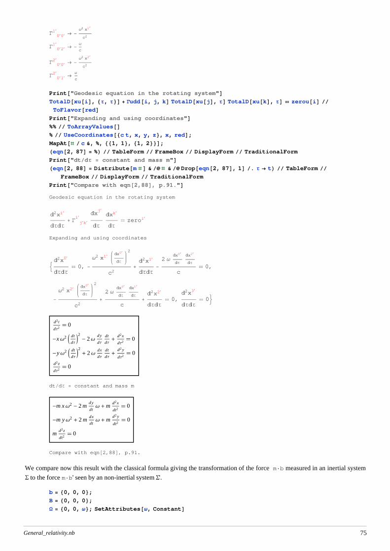
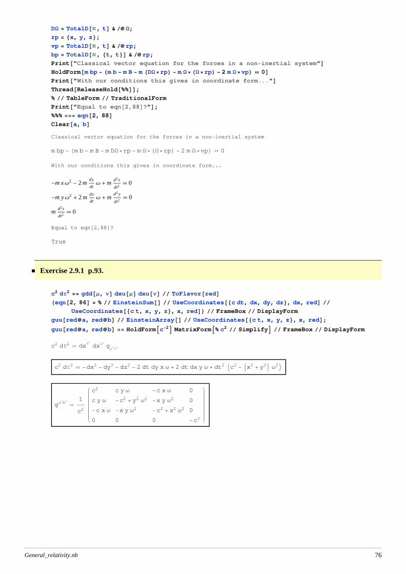
Print@"Classical vector equation for the forces in a non-inertial system"DHoldForm@m bp - Hm b - m B - m HDWrpL - m WHWrpL - 2 m WvpL 0DPrint@"With our conditions this gives in coordinate form..."DThread@ReleaseHold@%%DD;% TableForm TraditionalForm

Print@"Equal to eqn@2,88D?"D;%%% === eqn@2, 88DClear@a, bDClassical vector equation for the forces in a non-inertial system

m bp - Hm b - m B - m DWrp - m WHWrpL - 2 m WvpL 0

With our conditions this gives in coordinate form...

-m x Ω2 - 2 mâ y

âtΩ + m

â2 x

ât2 0

-m y Ω2 + 2 mâx

âtΩ + m

â2 y

ât2 0

mâ2z

ât2 0

Equal to eqn@2,88D?True

Exercise 2.9.1 p.93.

c2 dΤ2 == gdd@Μ, ΝD dxu@ΜD dxu@ΝD ToFlavor@redDHeqn@2, 86D = % EinsteinSum@D UseCoordinates@8c dt, dx, dy, dz<, dx, redD UseCoordinates@8c t, x, y, z<, x, redDL FrameBox DisplayForm

guu@reda, redbD EinsteinArray@D UseCoordinates@8c t, x, y, z<, x, redD;guu@reda, redbD == HoldFormAc-2E MatrixFormA% c2 SimplifyE FrameBox DisplayForm

c2 dΤ2 dxΜ¢

dxΝ¢gΜ¢Ν¢

c2 dΤ2 -dx2 - dy2 - dz2 - 2 dt dy x Ω + 2 dt dx y Ω + dt2 Ic2 - Ix2 + y2M Ω2M

ga¢b¢

1

c2

c2 c y Ω -c x Ω 0

c y Ω -c2 + y2 Ω2 -x y Ω2 0

-c x Ω -x y Ω2 -c2 + x2 Ω2 0

0 0 0 -c2


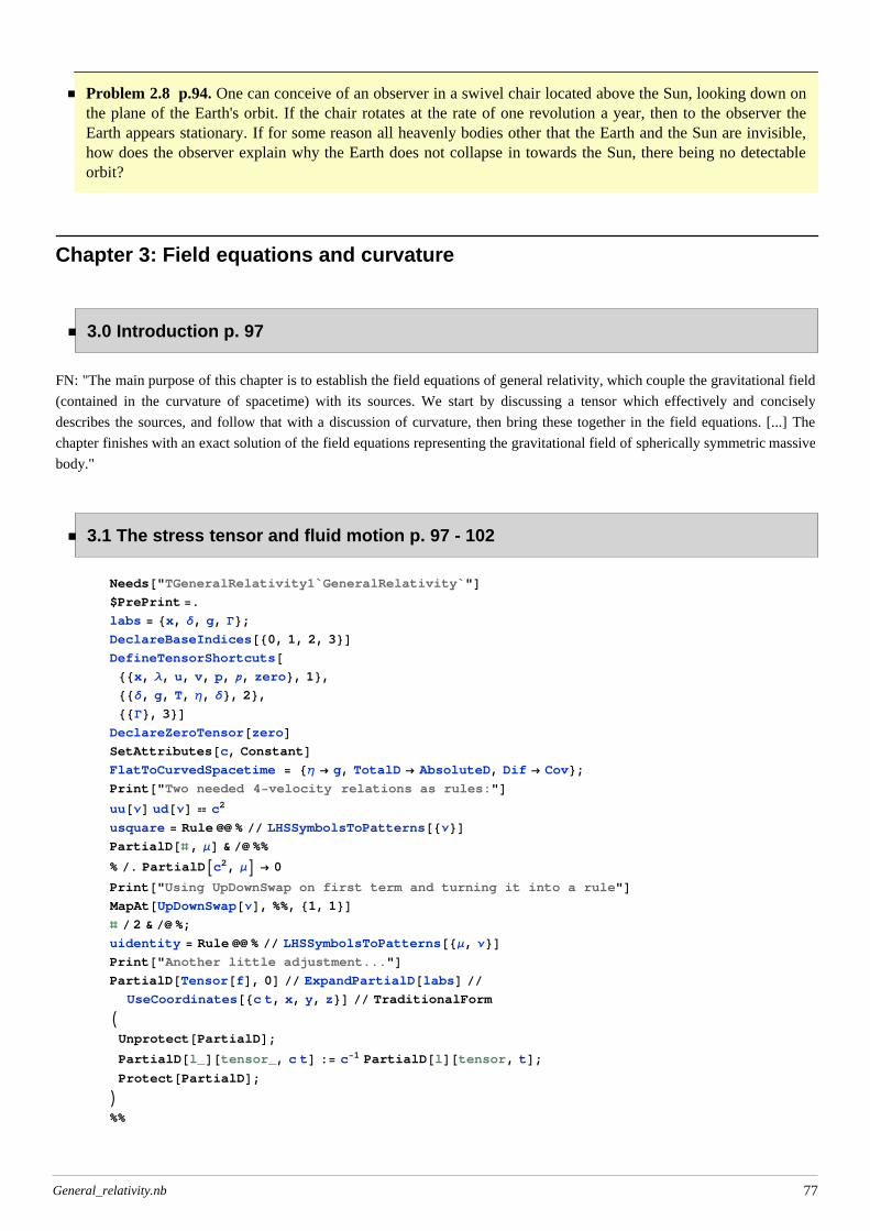
Problem 2.8 p.94. One can conceive of an observer in a swivel chair located above the Sun, looking down onthe plane of the Earth's orbit. If the chair rotates at the rate of one revolution a year, then to the observer theEarth appears stationary. If for some reason all heavenly bodies other that the Earth and the Sun are invisible,how does the observer explain why the Earth does not collapse in towards the Sun, there being no detectableorbit?

Chapter 3: Field equations and curvature


FN: "The main purpose of this chapter is to establish the field equations of general relativity, which couple the gravitational field

(contained in the curvature of spacetime) with its sources. We start by discussing a tensor which effectively and concisely

describes the sources, and follow that with a discussion of curvature, then bring these together in the field equations. [...] The

chapter finishes with an exact solution of the field equations representing the gravitational field of spherically symmetric massive

body."

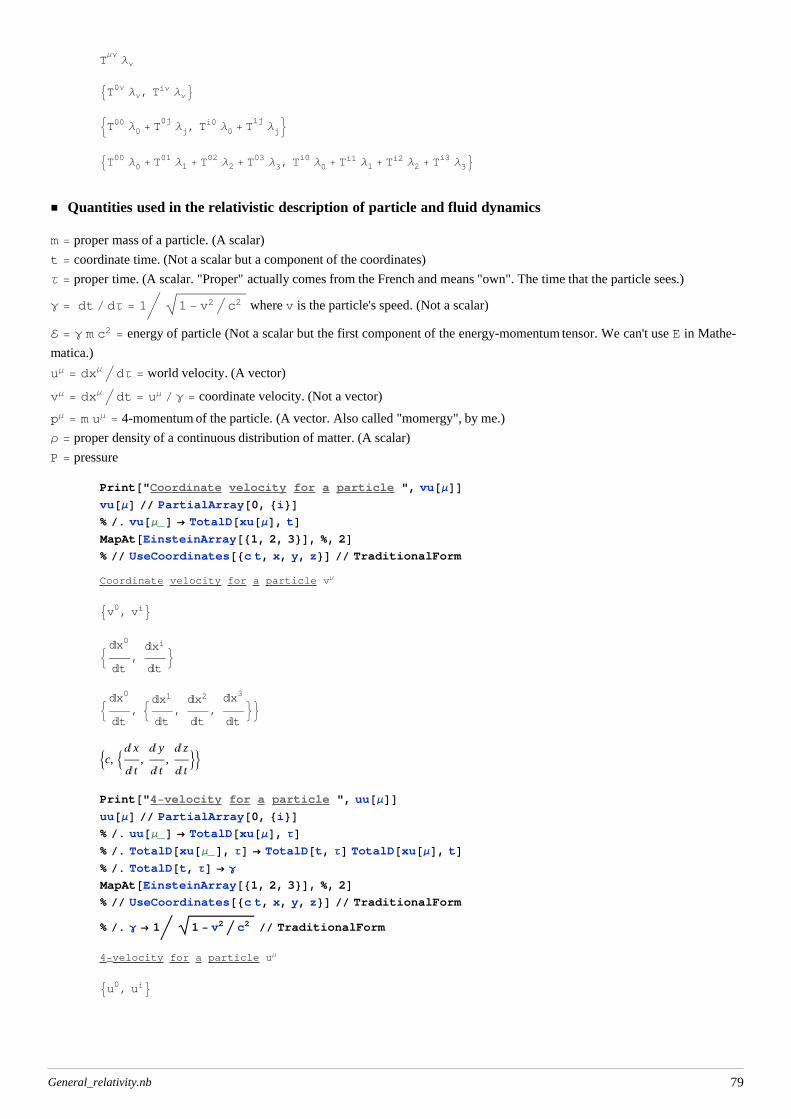
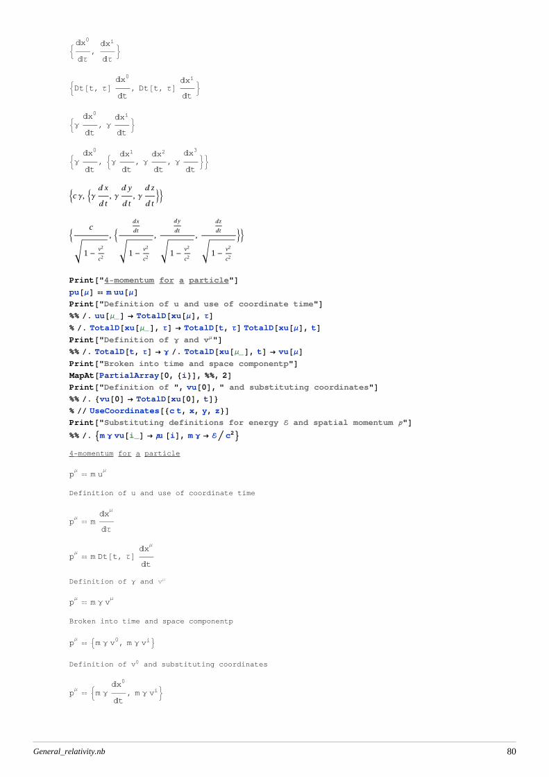
3.1 The stress tensor and fluid motion p. 97 - 102


labs = 8x, ∆, g, G<;DeclareBaseIndices@80, 1, 2, 3<DDefineTensorShortcuts@88x, Λ, u, v, p, p, zero<, 1<,88∆, g, T, Η, ∆<, 2<,88G<, 3<DDeclareZeroTensor@zeroDSetAttributes@c, ConstantDFlatToCurvedSpacetime = 8Η ® g, TotalD ® AbsoluteD, Dif ® Cov<;Print@"Two needed 4-velocity relations as rules:"Duu@ΝD ud@ΝD c2

usquare = Rule % LHSSymbolsToPatterns@8Ν<DPartialD@ð, ΜD & %%

% . PartialDAc2, ΜE ® 0

Print@"Using UpDownSwap on first term and turning it into a rule"DMapAt@UpDownSwap@ΝD, %%, 81, 1<Dð 2 & %;

uidentity = Rule % LHSSymbolsToPatterns@8Μ, Ν<DPrint@"Another little adjustment..."DPartialD@Tensor@fD, 0D ExpandPartialD@labsD

UseCoordinates@8c t, x, y, z<D TraditionalFormIUnprotect@PartialDD;PartialD@l_D@tensor_, c tD := c-1 PartialD@lD@tensor, tD;Protect@PartialDD;M

%%


Two needed 4-velocity relations as rules:

uΝ uΝ c2

uΝ_ uΝ_

® c2

uΝ uΝ,Μ + uΝ u ,ΜΝ

PartialDAc2, ΜEuΝ uΝ,Μ + uΝ u ,Μ

Ν 0

Using UpDownSwap on first term and turning it into a rule

2 uΝ u ,ΜΝ

0

uΝ_ u ,Μ_Ν_

® 0

Another little adjustment...

¶ f

¶c t

¶tf

c

Expanding the temporal and spatial parts of a tensor expressions

We can expand a 4-vector as follows...

Λu@ΜDΛu@ΜD EinsteinArray@DΛu@ΜD EinsteinArray@80<DΛu@ΜD EinsteinArray@81, 2, 3<DΛu@ΜD PartialArray@0, 8i<DMapAt@EinsteinArray@81, 2, 3<D, %, 2DH8Λ0, Λs< = %%L FullForm

Λs EinsteinArray@81, 2, 3<DΛ

Μ

9Λ0, Λ1, Λ2, Λ3=9Λ0=9Λ1, Λ2, Λ3=9Λ0, Λi=9Λ0, 9Λ1, Λ2, Λ3==List@Tensor@\[Lambda], List@0D, List@VoidDD, Tensor@\[Lambda], List@iD, List@VoidDDD9Λ1, Λ2, Λ3=

Mixed expansions. The number of separate parts goes as 2n where n is the number of free indices plus the number of dummy

pairs.

Tuu@Μ, ΝD Λd@ΝD% PartialArray@0, 8i<D% PartialSum@0, 8j<D%% EinsteinSum@D


TΜΝ

ΛΝ

9T0Ν ΛΝ, TiΝ ΛΝ=:T00 Λ0 + T

0jΛj, Ti0 Λ0 + T

ijΛj>

9T00 Λ0 + T01 Λ1 + T02 Λ2 + T03 Λ3, Ti0 Λ0 + Ti1 Λ1 + Ti2 Λ2 + Ti3 Λ3= Quantities used in the relativistic description of particle and fluid dynamics

m = proper mass of a particle. (A scalar)

t = coordinate time. (Not a scalar but a component of the coordinates)

Τ = proper time. (A scalar. "Proper" actually comes from the French and means "own". The time that the particle sees.)

Γ = dt dΤ = 1 1 - v2 c2 where v is the particle's speed. (Not a scalar)

E = Γ m c2 = energy of particle (Not a scalar but the first component of the energy-momentum tensor. We can't use E in Mathe-

matica.)

uΜ = dxΜ dΤ = world velocity. (A vector)

vΜ = dxΜ dt = uΜ Γ = coordinate velocity. (Not a vector)

pΜ = m uΜ = 4-momentum of the particle. (A vector. Also called "momergy", by me.)

Ρ = proper density of a continuous distribution of matter. (A scalar)

P = pressure

Print@"Coordinate velocity for a particle ", vu@ΜDDvu@ΜD PartialArray@0, 8i<D% . vu@Μ_D ® TotalD@xu@ΜD, tDMapAt@EinsteinArray@81, 2, 3<D, %, 2D% UseCoordinates@8c t, x, y, z<D TraditionalForm

Coordinate velocity for a particle vΜ

9v0, vi=: âx0

ât,

âxi

ât>

: âx0

ât, : âx1

ât,

âx2

ât,

âx3

ât>>

:c, : â x

â t,

â y

â t,

â z

â t>>

Print@"4-velocity for a particle ", uu@ΜDDuu@ΜD PartialArray@0, 8i<D% . uu@Μ_D ® TotalD@xu@ΜD, ΤD% . TotalD@xu@Μ_D, ΤD ® TotalD@t, ΤD TotalD@xu@ΜD, tD% . TotalD@t, ΤD ® Γ

MapAt@EinsteinArray@81, 2, 3<D, %, 2D% UseCoordinates@8c t, x, y, z<D TraditionalForm

% . Γ ® 1 1 - v2 c2 TraditionalForm

4-velocity for a particle uΜ

9u0, ui=


: âx0

âΤ,

âxi

âΤ>

:Dt@t, ΤD âx0

ât, Dt@t, ΤD âxi

ât>

:Γâx0

ât, Γ

âxi

ât>

:Γâx0

ât, :Γ

âx1

ât, Γ

âx2

ât, Γ

âx3

ât>>

:c Γ, :Γâ x

â t, Γ

â y

â t, Γ

â z

â t>>

: c

1 -v2

c2

, :âx

ât

1 -v2

c2

,

â y

ât

1 -v2

c2

,

âz

ât

1 -v2

c2

>>

Print@"4-momentum for a particle"Dpu@ΜD m uu@ΜDPrint@"Definition of u and use of coordinate time"D%% . uu@Μ_D ® TotalD@xu@ΜD, ΤD% . TotalD@xu@Μ_D, ΤD ® TotalD@t, ΤD TotalD@xu@ΜD, tDPrint@"Definition of Γ and vΜ"D%% . TotalD@t, ΤD ® Γ . TotalD@xu@Μ_D, tD ® vu@ΜDPrint@"Broken into time and space componentp"DMapAt@PartialArray@0, 8i<D, %%, 2DPrint@"Definition of ", vu@0D, " and substituting coordinates"D%% . 8vu@0D ® TotalD@xu@0D, tD<% UseCoordinates@8c t, x, y, z<DPrint@"Substituting definitions for energy E and spatial momentum p"D%% . 9m Γ vu@i_D ® pu @iD, m Γ ® E c2=4-momentum for a particle

pΜ

m uΜ

Definition of u and use of coordinate time

pΜ

mâx

Μ

âΤ

pΜ

m Dt@t, ΤD âxΜ

ât

Definition of Γ and vΜ

pΜ

m Γ vΜ

Broken into time and space componentp

pΜ

9m Γ v0, m Γ vi=Definition of v0 and substituting coordinates

pΜ

:m Γâx0

ât, m Γ vi>


pΜ

9c m Γ, m Γ vi=Substituting definitions for energy E and spatial momentum p

pΜ

: Ec, pi>

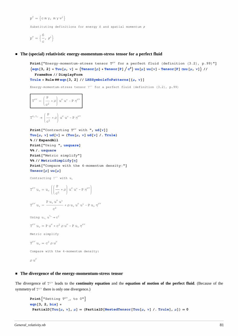
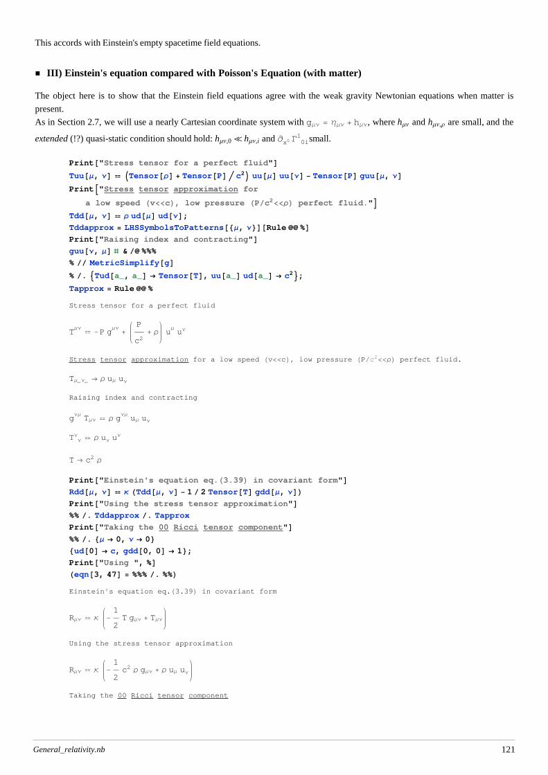
The (special) relativistic energy-momentum-stress tensor for a perfect fluid

Print@"Energy-momentum-stress tensor TΜΝ for a perfect fluid Hdefinition H3.2L, p.99L"DIeqn@3, 2D = Tuu@Μ, ΝD ITensor@ΡD + Tensor@PD c2M uu@ΜD uu@ΝD - Tensor@PD Ηuu@Μ, ΝDM FrameBox DisplayForm

Trule = Rule eqn@3, 2D LHSSymbolsToPatterns@8Μ, Ν<DEnergy-momentum-stress tensor TΜΝ for a perfect fluid Hdefinition H3.2L, p.99L

TΜΝ

P

c2+ Ρ u

ΜuΝ - P Η

ΜΝ

TΜ_Ν_

®P

c2+ Ρ u

ΜuΝ - P Η

ΜΝ

Print@"Contracting TΜΝ with ", ud@ΝDDTuu@Μ, ΝD ud@ΝD HTuu@Μ, ΝD ud@ΝD . TruleL% ExpandAll

Print@"Using ", usquareD%% . usquare

Print@"Metric simplify"D%% MetricSimplify@ΗDPrint@"Compare with the 4-momentum density:"DTensor@ΡD uu@ΜDContracting TΜΝ with uΝ

TΜΝuΝ uΝ

P

c2+ Ρ u

ΜuΝ - P Η

ΜΝ

TΜΝuΝ

P uΝ uΜuΝ

c2+ Ρ uΝ u

ΜuΝ - P uΝ Η

ΜΝ

Using uΝ_ uΝ_

® c2

TΜΝuΝ P u

Μ+ c2 Ρ u

Μ- P uΝ Η

ΜΝ

Metric simplify

TΜΝuΝ c2 Ρ u

Μ

Compare with the 4-momentum density:

Ρ uΜ

The divergence of the energy-momentum-stress tensor

The divergence of TΜΝ leads to the continuity equation and the equation of motion of the perfect fluid. (Because of the

symmetry of TΜΝ there is only one divergence.)

PrintA"Setting TΜΝ,Μ to 0"E

eqn@3, 2, bisD =

PartialD@Tuu@Μ, ΝD, ΜD HPartialD@NestedTensor@Tuu@Μ, ΝD . TruleD, ΜDL 0


PartialD@Tuu@Μ, ΝD, ΜD HPartialD@NestedTensor@Tuu@Μ, ΝD . TruleD, ΜDL 0

Print@"Expanding and using constancy of Η"D%% UnnestTensor

% . PartialD@Ηuu@_, _D, _D ® 0

Print@"Dropping first equation and expanding"Deqn@3, 3D = HDrop@%%, 1D ExpandAllLSetting TΜΝ

,Μ to 0

T ,ΜΜΝ

P

c2+ Ρ u

ΜuΝ - P Η

ΜΝ

,Μ

0

Expanding and using constancy of Η

T ,ΜΜΝ

P

c2+ Ρ IuΝ u ,Μ

Μ+ u

Μu ,Μ

Ν M - P,Μ ΗΜΝ

- P Η ,ΜΜΝ

+ uΜuΝ

P,Μ

c2+ Ρ,Μ 0

T ,ΜΜΝ

P

c2+ Ρ IuΝ u ,Μ

Μ+ u

Μu ,Μ

Ν M - P,Μ ΗΜΝ

+ uΜuΝ

P,Μ

c2+ Ρ,Μ 0

Dropping first equation and expanding

P,Μ uΜuΝ

c2+P uΝ u ,Μ

Μ

c2+ Ρ uΝ u ,Μ

Μ+P u

Μu ,Μ

Ν

c2+ Ρ u

Μu ,Μ

Ν- P,Μ Η

ΜΝ+ u

ΜuΝ Ρ,Μ 0

Print@"IL Equation of continuity"DPrintA"Contracting TΜΝ

,Μ with ", ud@ΝDEDistribute@ð ud@ΝDD & eqn@3, 3DPrint@"Using ", usquare, " and ", uidentityD%% . 8usquare, uidentity<MapAt@MapLevelParts@MetricSimplify@ΗD, 883, 4<<D, %, 81, 4<Deqn@3, 5, 1D = %;

ð c2 & %% Simplify

Print@"Check proposed simplification"DHeqn@3, 5D = First@%%@@1DDD +

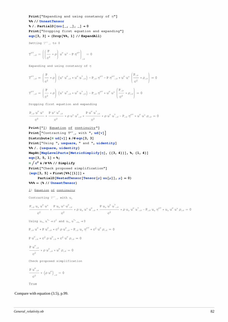
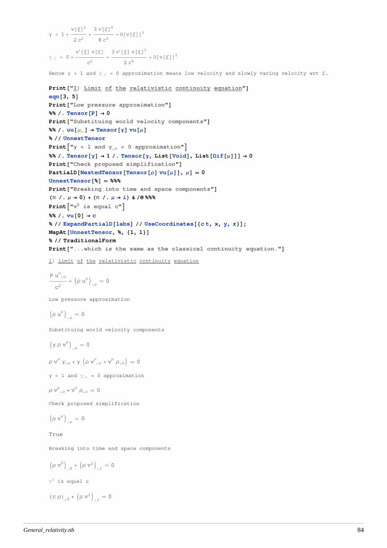
PartialD@NestedTensor@Tensor@ΡD uu@ΜDD, ΜD 0L%%% H% UnnestTensorLIL Equation of continuity

Contracting TΜΝ,Μ with uΝ

P,Μ uΝ uΜuΝ

c2+P uΝ u

Ν u ,ΜΜ

c2+ Ρ uΝ u

Ν u ,ΜΜ

+P uΝ u

Μu ,Μ

Ν

c2+ Ρ uΝ u

Μu ,Μ

Ν- P,Μ uΝ Η

ΜΝ+ uΝ u

ΜuΝ Ρ,Μ 0

Using uΝ_ uΝ_

® c2 and uΝ_ u ,Μ_Ν_

® 0

P,Μ uΜ

+ P u ,ΜΜ

+ c2 Ρ u ,ΜΜ

- P,Μ uΝ ΗΜΝ

+ c2 uΜ

Ρ,Μ 0

P u ,ΜΜ

+ c2 Ρ u ,ΜΜ

+ c2 uΜ

Ρ,Μ 0

P u ,ΜΜ

c2+ Ρ u ,Μ

Μ+ u

ΜΡ,Μ 0

Check proposed simplification

P u ,ΜΜ

c2+ IΡ u

ΜM,Μ

0

True

Compare with equation (3.5), p.99.


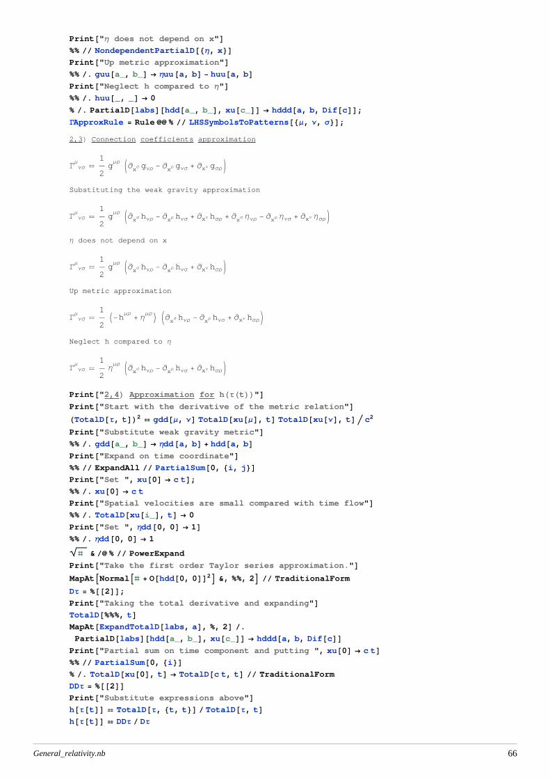
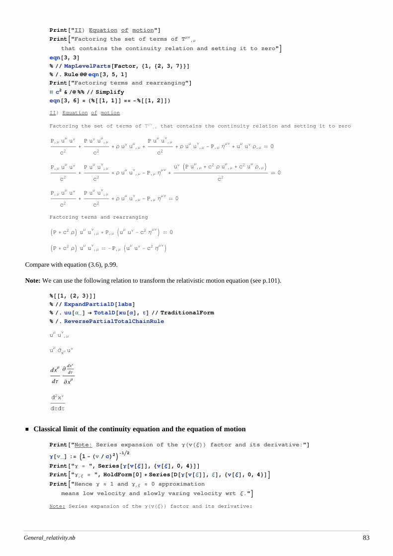
Print@"IIL Equation of motion"DPrintA"Factoring the set of terms of TΜΝ

,Μ

that contains the continuity relation and setting it to zero"Eeqn@3, 3D% MapLevelParts@Factor, 81, 82, 3, 7<<D% . Rule eqn@3, 5, 1DPrint@"Factoring terms and rearranging"Dð c2 & %% Simplify

eqn@3, 6D = H%@@1, 1DD == -%@@1, 2DDLIIL Equation of motion

Factoring the set of terms of TΜΝ,Μ that contains the continuity relation and setting it to zero

P,Μ uΜuΝ

c2+P uΝ u ,Μ

Μ

c2+ Ρ uΝ u ,Μ

Μ+P u

Μu ,Μ

Ν

c2+ Ρ u

Μu ,Μ

Ν- P,Μ Η

ΜΝ+ u

ΜuΝ Ρ,Μ 0

P,Μ uΜuΝ

c2+P u

Μu ,Μ

Ν

c2+ Ρ u

Μu ,Μ

Ν- P,Μ Η

ΜΝ+uΝ IP u ,Μ

Μ+ c2 Ρ u ,Μ

Μ+ c2 u

ΜΡ,ΜM

c2 0

P,Μ uΜuΝ

c2+P u

Μu ,Μ

Ν

c2+ Ρ u

Μu ,Μ

Ν- P,Μ Η

ΜΝ 0

Factoring terms and rearranging

IP + c2 ΡM uΜu ,Μ

Ν+ P,Μ IuΜ

uΝ - c2 ΗΜΝM 0


Ν -P,Μ IuΜ

uΝ - c2 ΗΜΝM


Note: We can use the following relation to transform the relativistic motion equation (see p.101).

%@@1, 82, 3<DD% ExpandPartialD@labsD% . uu@Α_D ® TotalD@xu@ΑD, ΤD TraditionalForm

% . ReversePartialTotalChainRule

uΜu ,Μ

Ν

uΜ

¶xΜ uΝ

âxΜ

âΤ

¶âxΝ

âΤ

¶ xΜ

â2xΝ

âΤâΤ

Classical limit of the continuity equation and the equation of motion

Print@"Note: Series expansion of the ΓHvHΞLL factor and its derivative:"DΓ@v_D := I1 - Hv cL2M-12Print@"Γ = ", Series@Γ@v@ΞDD, 8v@ΞD, 0, 4<DDPrintA"Γ,Ξ = ", HoldForm@0D + Series@D@Γ@v@ΞDD, ΞD, 8v@ΞD, 0, 4<DEPrintA"Hence Γ » 1 and Γ,Ξ » 0 approximation

means low velocity and slowly varing velocity wrt Ξ."ENote: Series expansion of the ΓHvHΞLL factor and its derivative:


Γ = 1 +v@ΞD2

2 c2+3 v@ΞD4

8 c4+ O@v@ΞDD5

Γ,Ξ = 0 +v¢@ΞD v@ΞD

c2+3 v¢@ΞD v@ΞD3

2 c4+ O@v@ΞDD5

Hence Γ » 1 and Γ,Ξ » 0 approximation means low velocity and slowly varing velocity wrt Ξ.

Print@"IL Limit of the relativistic continuity equation"Deqn@3, 5DPrint@"Low pressure approximation"D%% . Tensor@PD ® 0

Print@"Substituing world velocity components"D%% . uu@Μ_D ® Tensor@ΓD vu@ΜD% UnnestTensor

PrintA"Γ » 1 and Γ,Μ » 0 approximation"E%% . Tensor@ΓD ® 1 . Tensor@Γ, List@VoidD, List@Dif@ΜDDD ® 0

Print@"Check proposed simplification"DPartialD@NestedTensor@Tensor@ΡD vu@ΜDD, ΜD 0

UnnestTensor@%D %%%

Print@"Breaking into time and space components"DHð . Μ ® 0L + Hð . Μ ® iL & %%%

PrintA"v0 is equal c"E%% . vu@0D ® c

% ExpandPartialD@labsD UseCoordinates@8c t, x, y, z<D;MapAt@UnnestTensor, %, 81, 1<D% TraditionalForm

Print@"...which is the same as the classical continuity equation."DIL Limit of the relativistic continuity equation

P u ,ΜΜ

c2+ IΡ u

ΜM,Μ

0

Low pressure approximation

IΡ uΜM

,Μ 0

Substituing world velocity components

IΓ Ρ vΜM

,Μ 0

Ρ vΜ

Γ,Μ + Γ IΡ v ,ΜΜ

+ vΜ

Ρ,ΜM 0

Γ » 1 and Γ,Μ » 0 approximation

Ρ v ,ΜΜ

+ vΜ

Ρ,Μ 0

Check proposed simplification

IΡ vΜM

,Μ 0

True

Breaking into time and space components

IΡ v0M,0

+ IΡ viM,i

0

v0 is equal c

Hc ΡL,0 + IΡ viM,i

0


¶tΡ + ¶xi IΡ viM 0

¶ Ρ

¶ t+

¶ HΡ viL¶ xi

0

...which is the same as the classical continuity equation.


Print@"IIL Limit of the relativistic equation of motion for a perfect fluid"Deqn@3, 6DPrint@"Low pressure approximation"D%% . Tensor@PD ® 0

Print@"Substituing world velocity components"D%% . uu@Μ_D ® Tensor@ΓD vu@ΜD . PartialD@uu@ΝD, ΜD ® PartialD@Tensor@ΓD vu@ΝD, ΜDPrintA"Γ » 1 and Γ,Μ » 0 approximation"E%% . Tensor@ΓD ® 1 . Tensor@Γ, List@VoidD, List@Dif@ΜDDD ® 0

Print@"Expand, separate into time and space components"D%% ExpandAll

% PartialSum@0, 8j<D;% PartialArray@0, 8i<D Thread

Print@"Simplify Η, ",

vu@0D ® c, ", ",

vu@i_D vu@j_D ® 0, ", ", PartialD@vu@0D, j_D ® 0D%% . Ηuu@0, 0D ® 1 . Ηuu@i_, j_D ; i 0 ê j 0 ® 0;

% . vu@0D ® c . vu@i_D vu@j_D ® 0 . PartialD@vu@0D, j_D ® 0

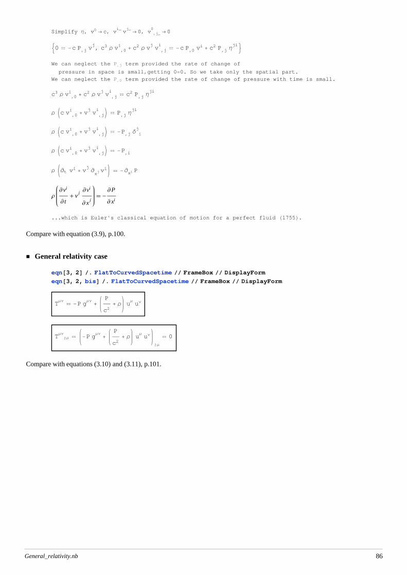
PrintA"We can neglect the P,j term provided the rate of change of pressure in space

is small,getting 0=0. So we take only the spatial part.\nWe can neglect

the P,0 term provided the rate of change of pressure with time is small."E%%@@2DD . Tensor@P, List@VoidD, List@Dif@0DDD ® 0

ð c-2 & % Simplify

% . Ηuu@j, iD ® -∆ud@j, iD% KroneckerAbsorb@∆D% ExpandPartialD@labsD UseCoordinates@8c t, x, y, z<D;% MapLevelParts@Factor, 81, 81, 2<<D% TraditionalForm

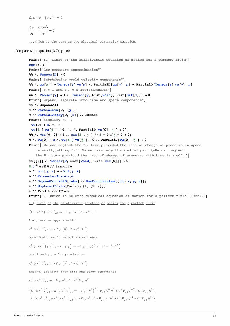
Print@"...which is Euler's classical equation of motion for a perfect fluid H1755L."DIIL Limit of the relativistic equation of motion for a perfect fluid


Ν -P,Μ IuΜ

uΝ - c2 ΗΜΝM

Low pressure approximation

c2 Ρ uΜu ,Μ

Ν -P,Μ IuΜ

uΝ - c2 ΗΜΝM

Substituing world velocity components

c2 Γ Ρ vΜ IΓ v ,Μ

Ν+ vΝ Γ,ΜM -P,Μ IHΓL2 v

ΜvΝ - c2 Η

ΜΝMΓ » 1 and Γ,Μ » 0 approximation

c2 Ρ vΜv ,Μ

Ν -P,Μ IvΜ

vΝ - c2 ΗΜΝM

Expand, separate into time and space components

c2 Ρ vΜv ,Μ

Ν -P,Μ v

ΜvΝ + c2 P,Μ Η

ΜΝ

:c2 Ρ v0 v ,00 + c2 Ρ v

jv ,j0

-P,0 Iv0M2- P,j v

0 vj

+ c2 P,0 Η00 + c2 P,j Ηj0,

c2 Ρ v0 v ,0i + c2 Ρ v

jv ,ji

-P,0 v0 vi - P,j v

i vj

+ c2 P,0 Η0i + c2 P,j Ηji>


Simplify Η, v0 ® c, vi_vj_

® 0, v ,j_0

® 0

:0 -c P,j vj, c3 Ρ v ,0

i + c2 Ρ vjv ,ji

-c P,0 vi + c2 P,j Η

ji>We can neglect the P,j term provided the rate of change of

pressure in space is small,getting 0=0. So we take only the spatial part.

We can neglect the P,0 term provided the rate of change of pressure with time is small.

c3 Ρ v ,0i + c2 Ρ v

jv ,ji

c2 P,j Ηji

Ρ Jc v ,0i + v

jv ,ji N P,j Η

ji

Ρ Jc v ,0i + v

jv ,ji N -P,j ∆ i

j

Ρ Jc v ,0i + v

jv ,ji N -P,i

Ρ K¶t vi + vj

¶xjviO -¶xi P

Ρ¶vi

¶ t+ v

j ¶vi

¶ xj

-¶ P

¶ xi

...which is Euler's classical equation of motion for a perfect fluid H1755L.Compare with equation (3.9), p.100.

General relativity case

eqn@3, 2D . FlatToCurvedSpacetime FrameBox DisplayForm

eqn@3, 2, bisD . FlatToCurvedSpacetime FrameBox DisplayForm

TΜΝ

-P gΜΝ

+P

c2+ Ρ u

ΜuΝ

T ;ΜΜΝ

-P gΜΝ

+P

c2+ Ρ u

ΜuΝ

;Μ

0

Compare with equations (3.10) and (3.11), p.101.


3.2 The curvature tensor and related tensors p. 102 - 105


labs = 8x, ∆, g, G<;DeclareBaseIndices@80, 1, 2, 3<DMyRed = StyleForm@Superscript@ð, "¢"D, FontColor ® RGBColor@1, 0, 0DD &;

DeclareIndexFlavor@8red, MyRed<DDefineTensorShortcuts@88x, Λ, e<, 1<,88∆, g, R, G, Τ<, 2<,88G, R, Τ<, 3<,88R<, 4<,88R<, 5<DH* - - - *LRiemannToChristoffelRule = LHSSymbolsToPatterns@8a, b, c, d<DRiemannRule

ChristoffelToRiemannRule = LHSSymbolsToPatterns@8a, b, c, d, e<DReverseRiemannRule

ChDoRule = LHSSymbolsToPatterns@8a, b, c<D@ChristoffelDownRuleDPaMeRule = LHSSymbolsToPatterns@8a, b, c<D@PartialMetricRuleDR a_b_c_d_

® -G ced G ab

e + G bed G ac

e - ¶xc G abd + ¶xb G ac

d

-G c_e_d_

G a_b_e_

+ G b_e_d_

G a_c_e_

- ¶xc_ G a_b_

d_+ ¶

xb_ G a_c_

d_® R abc

d

Ga_b_c_ ®1


ga_b_,c_ ® Gabc + Gbac

1) Curvature tensor R abcd from commutator of covariant differentiation

Print@"Commutator of the covariant differentiation of a covariant vector field ", Λd@aDDcommutator = CovariantD@Λd@aD, 8b, c<D - CovariantD@Λd@aD, 8c, b<DPrint@"Expanding and collecting ", Λd@dD, " terms"D%% ExpandCovariantD@labs, 8d, e<DCollect@%, Λd@dDDPrint@"Using symmetry of G"D%% SymmetrizeSlots@G, 3, 81, 82, 3<<DPrint@"Last terms cancel out"D%% MapLevelParts@SimplifyTensorSum, 882, 4<<D;% MapLevelParts@SimplifyTensorSum, 882, 3<<DPrint@"Substituting the definition of the Curvature tensor"Dcommutator == Heqn@3, 12D = %% . ChristoffelToRiemannRuleL FrameBox DisplayForm

Print@"Dies ist die Ricci-Identität. Ricci identity."DCommutator of the covariant differentiation of a covariant vector field Λa

Λa;b;c - Λa;c;b

Expanding and collecting Λd terms

-Λd ¶xc G bad + Λd ¶xb G ca

d + G bce I-G ea

d Λd + ¶xe ΛaM - G cbe I-G ea

d Λd + ¶xe ΛaM +

G cad ¶xb Λd - G ba

d ¶xc Λd - G cae J-G be

d Λd + ¶xb ΛeN + G bae I-G ce

d Λd + ¶xc ΛeM


Λd J-G ced G ba

e - G ead G bc

e + G bed G ca

e + G ead G cb

e - ¶xc G bad + ¶xb G ca

d N +

G bce ¶xe Λa - G cb

e ¶xe Λa + G cad ¶xb Λd - G ba

d ¶xc Λd - G cae ¶xb Λe + G ba

e ¶xc Λe

Using symmetry of G

Λd J-G ced G ab

e + G bed G ac


d N + G acd ¶xb Λd - G ab

d ¶xc Λd - G ace ¶xb Λe + G ab

e ¶xc Λe

Last terms cancel out

Λd J-G ced G ab

e + G bed G ac


d NSubstituting the definition of the Curvature tensor

Λa;b;c - Λa;c;b R abcd Λd

Dies ist die Ricci-Identität. Ricci identity.

If the curvature tensor is identically zero, then covariant differentiation is (generally) commutative. In flat spacetime we can

always find a coordinate system in which all the connection coefficients are zero, namely the Cartesian form of the Minkowski

metric. Therefore the curvature tensor will be zero, not only in the Cartesian form of the metric, but in all coordinate systems.

The connection coefficients are not necessarily zero in other coordinate systems. They are not tensors.

2) Der vollständig kovariante Riemannsche Krümmungstensor (down curvature tensor) Rabcd

Wir wollen hier verschiedene Formen des vollständig kovarianten Riemannschen Krümmungstensors berechnen.

Print@"Curvature tensor definition"DRuddd@f, b, c, dD == HRuddd@f, b, c, dD . RiemannToChristoffelRuleLPrint@"Lowering the index"DDistribute@gdd@a, fD ð D & %%

step1 = CovariantRiemannRule = % MetricSimplify@gDCurvature tensor definition

R bcdf G bd

e G cef - G bc

e G def - ¶xd G bc

f + ¶xc G bdf

Lowering the index

gaf R bcdf gaf G bd

e G cef - gaf G bc

e G def - gaf ¶xd G bc

f + gaf ¶xc G bdf

Rabcd G bde Gace - G bc

e Gade - gaf ¶xd G bcf + gaf ¶xc G bd

f

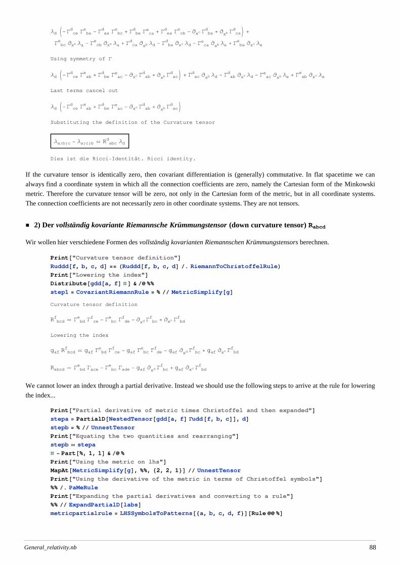
We cannot lower an index through a partial derivative. Instead we should use the following steps to arrive at the rule for lowering

the index...

Print@"Partial derivative of metric times Christoffel and then expanded"Dstepa = PartialD@NestedTensor@gdd@a, fD Gudd@f, b, cDD, dDstepb = % UnnestTensor

Print@"Equating the two quantities and rearranging"Dstepb stepa

ð - Part@%, 1, 1D & %

Print@"Using the metric on lhs"DMapAt@MetricSimplify@gD, %%, 82, 2, 1<D UnnestTensor

Print@"Using the derivative of the metric in terms of Christoffel symbols"D%% . PaMeRule

Print@"Expanding the partial derivatives and converting to a rule"D%% ExpandPartialD@labsDmetricpartialrule = LHSSymbolsToPatterns@8a, b, c, d, f<D@Rule %D


Partial derivative of metric times Christoffel and then expanded

Igaf G bcf M

,d

gaf,d G bcf + gaf G bc,d

f

Equating the two quantities and rearranging

gaf,d G bcf + gaf G bc,d

f Igaf G bcf M

,d

gaf G bc,df -gaf,d G bc

f + Igaf G bcf M

,d

Using the metric on lhs

gaf G bc,df -gaf,d G bc

f + Gabc,d

Using the derivative of the metric in terms of Christoffel symbols

gaf G bc,df -G bc

f IGafd + GfadM + Gabc,d

Expanding the partial derivatives and converting to a rule

gaf ¶xd G bcf -G bc

f IGafd + GfadM + ¶xd Gabc

ga_f_ ¶xd_ G b_c_

f_® -G bc

f IGafd + GfadM + ¶xd Gabc

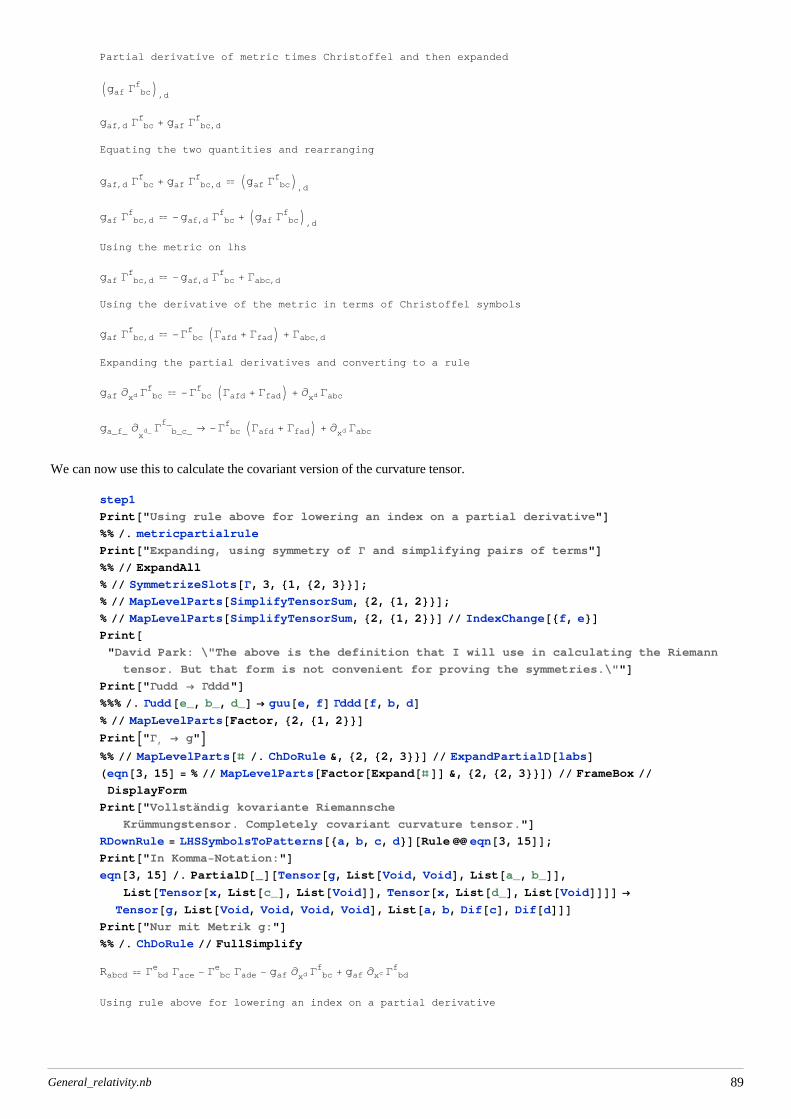
We can now use this to calculate the covariant version of the curvature tensor.

step1

Print@"Using rule above for lowering an index on a partial derivative"D%% . metricpartialrule

Print@"Expanding, using symmetry of G and simplifying pairs of terms"D%% ExpandAll

% SymmetrizeSlots@G, 3, 81, 82, 3<<D;% MapLevelParts@SimplifyTensorSum, 82, 81, 2<<D;% MapLevelParts@SimplifyTensorSum, 82, 81, 2<<D IndexChange@8f, e<DPrint@"David Park: \"The above is the definition that I will use in calculating the Riemann

tensor. But that form is not convenient for proving the symmetries.\""DPrint@"Gudd ® Gddd"D%%% . Gudd@e_, b_, d_D ® guu@e, fD Gddd@f, b, dD% MapLevelParts@Factor, 82, 81, 2<<DPrintA"G, ® g"E%% MapLevelParts@ð . ChDoRule &, 82, 82, 3<<D ExpandPartialD@labsDHeqn@3, 15D = % MapLevelParts@Factor@Expand@ð DD &, 82, 82, 3<<DL FrameBox DisplayForm

Print@"Vollständig kovariante Riemannsche

Krümmungstensor. Completely covariant curvature tensor."DRDownRule = LHSSymbolsToPatterns@8a, b, c, d<D@Rule eqn@3, 15DD;Print@"In Komma-Notation:"Deqn@3, 15D . PartialD@_D@Tensor@g, List@Void, VoidD, List@a_, b_DD,

List@Tensor@x, List@c_D, List@VoidDD, Tensor@x, List@d_D, List@VoidDDDD ®

Tensor@g, List@Void, Void, Void, VoidD, List@a, b, Dif@cD, Dif@dDDDPrint@"Nur mit Metrik g:"D%% . ChDoRule FullSimplify


e Gade - gaf ¶xd G bcf + gaf ¶xc G bd

f

Using rule above for lowering an index on a partial derivative



e Gade - G bdf IGafc + GfacM + G bc

f IGafd + GfadM - ¶xd Gabc + ¶xc Gabd

Expanding, using symmetry of G and simplifying pairs of terms


e Gade - G bdf Gafc + G bc

f Gafd - G bdf Gfac + G bc

f Gfad - ¶xd Gabc + ¶xc Gabd

Rabcd -G bde Geac + G bc

e Gead - ¶xd Gabc + ¶xc Gabd

David Park: "The above is the definition that I will use in calculating

the Riemann tensor. But that form is not convenient for proving the symmetries."

Gudd ® Gddd

Rabcd gef Gead Gfbc - gef Geac Gfbd - ¶xd Gabc + ¶xc Gabd

Rabcd gef IGead Gfbc - Geac GfbdM - ¶xd Gabc + ¶xc Gabd

G, ® g

Rabcd

gef IGead Gfbc - Geac GfbdM +1

2J-¶xb,xd gac - ¶xc,xd gba + ¶xa,xd gbcN +

1

2J¶xb,xc gad + ¶xc,xd gba - ¶xa,xc gbdN

Rabcd gef IGead Gfbc - Geac GfbdM +1

2J-¶xb,xd gac + ¶xb,xc gad + ¶xa,xd gbc - ¶xa,xc gbdN

Vollständig kovariante Riemannsche Krümmungstensor. Completely covariant curvature tensor.

In Komma-Notation:

Rabcd 1

2I-gac,b,d + gad,b,c + gbc,a,d - gbd,a,cM + gef IGead Gfbc - Geac GfbdM

Nur mit Metrik g:

Rabcd

1

4Igef II-gad,e + gae,d + ged,aM I-gbc,f + gbf,c + gfc,bM - H-gac,e + gae,c + gec,aL I-gbd,f + gbf,d + gfd,bMM +

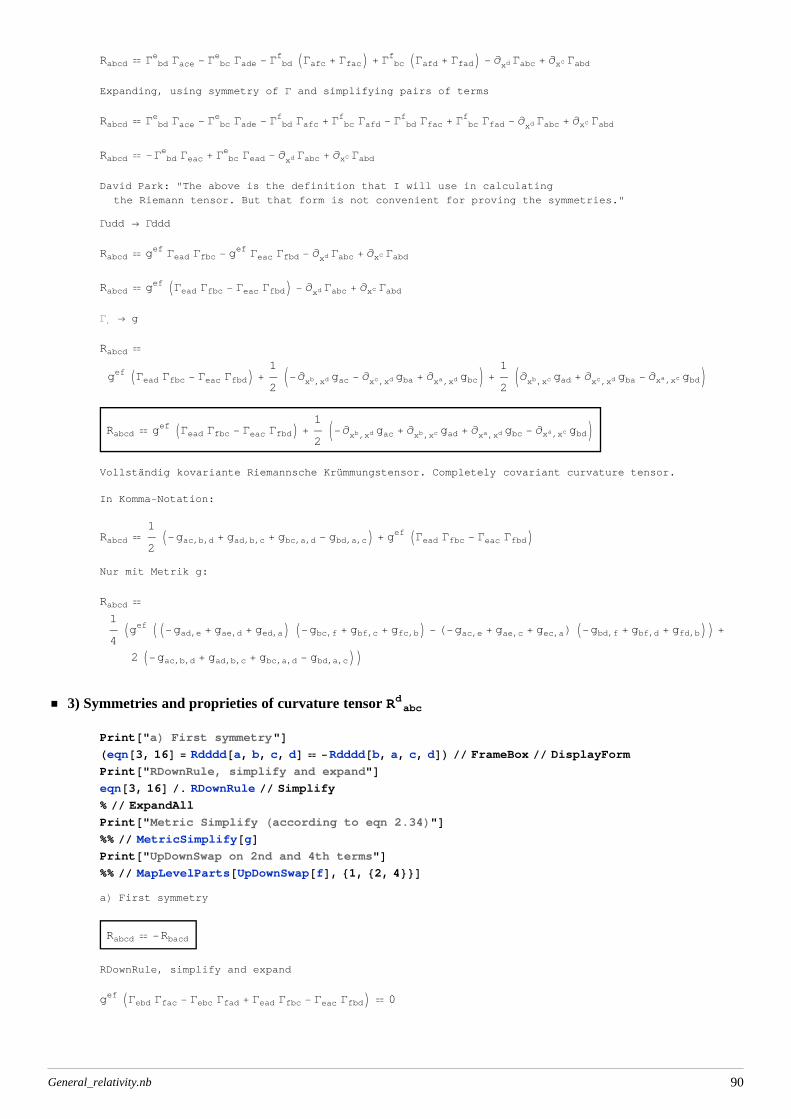
2 I-gac,b,d + gad,b,c + gbc,a,d - gbd,a,cMM 3) Symmetries and proprieties of curvature tensor R abc

d

Print@"aL First symmetry"DHeqn@3, 16D = Rdddd@a, b, c, dD -Rdddd@b, a, c, dDL FrameBox DisplayForm

Print@"RDownRule, simplify and expand"Deqn@3, 16D . RDownRule Simplify

% ExpandAll

Print@"Metric Simplify Haccording to eqn 2.34L"D%% MetricSimplify@gDPrint@"UpDownSwap on 2nd and 4th terms"D%% MapLevelParts@UpDownSwap@fD, 81, 82, 4<<DaL First symmetry

Rabcd -Rbacd

RDownRule, simplify and expand

gef IGebd Gfac - Gebc Gfad + Gead Gfbc - Geac GfbdM 0


gef Gebd Gfac - gef Gebc Gfad + gef Gead Gfbc - gef Geac Gfbd 0

Metric Simplify Haccording to eqn 2.34LG bdf Gfac - G bc

f Gfad + G adf Gfbc - G ac

f Gfbd 0

UpDownSwap on 2nd and 4th terms

True

Print@"bL Second symmetry"DHeqn@3, 17D = Rdddd@a, b, c, dD -Rdddd@a, b, d, cDL FrameBox DisplayForm

eqn@3, 17D . RDownRule Simplify

bL Second symmetry

Rabcd -Rabdc

True

Print@"cL Third symmetry"DHeqn@3, 18D = Rdddd@a, b, c, dD Rdddd@c, d, a, bDL FrameBox DisplayForm

PrintA"RDownRule, use g and G symmetries, simplify and expand"Eeqn@3, 18D . RDownRule SymmetrizeSlots@g, 2, 81, 81, 2<<D

SymmetrizeSlots@G, 3, 81, 82, 3<<D Simplify

% ExpandAll MetricSimplify@gDPrint@"UpDownSwap on second term"DMapAt@UpDownSwap@fD, %%, 881, 2<<DcL Third symmetry

Rabcd Rcdab

RDownRule, use g and G symmetries, simplify and expand

gef IGebc Gfad - Gead GfbcM 0

G bcf Gfad - G ad

f Gfbc 0

UpDownSwap on second term

True

Print@"dL Cyclic identity HExercise 3.2.2L"DHCyclicIdentity = Plus MapThread@Ruddd@a, Sequence ð D &,8Table@RotateLeft@8b, c, d<, iD, 8i, 0, 2<D<D 0L FrameBox DisplayForm

Print@"Expanding the terms to their definitions"DCyclicIdentity . RiemannToChristoffelRule

Print@"Using symmetry of G"D%% SymmetrizeSlots@G, 3, 81, 82, 3<<DdL Cyclic identity HExercise 3.2.2LR bcda + R cdb

a + R dbca 0

Expanding the terms to their definitions

-G dea G bc

e + G cea G bd

e + G dea G cb

e - G bea G cd

e - G cea G db

e +

G bea G dc

e - ¶xd G bca + ¶xc G bd

a + ¶xd G cba - ¶xb G cd

a - ¶xc G dba + ¶xb G dc

a 0

Using symmetry of G


True

Print@"eL Bianchi identity",

"\nAt any point P we can construct a geodesic coordinate system where"DredGrule = Gudd@a, b, cD ® 0 ToFlavor@redD LHSSymbolsToPatterns@8a, b, c<DPrint@"Definition of the curvature tensor at point P in the red coordinates and reindex"D

RiemannRule

% IndexChange@88d, a<, 8a, b<, 8b, c<, 8c, d<<D ToFlavor@redDPrint@"Unevaluating the partial derivatives"D%% . HoldPattern@PartialD@labs_D@t_Tensor, Tensor@x, 8a_<, 8Void<DDD ¦ PartialD@t, aDPrint@"Taking the partial derivative of each side"DPartialD@ð, redeD & %%

Print@"Setting the Christoffel symbols to zero, but not their derivatives"Dstep1 = %% . redGrule

Print@"But in the geodesic coordinates system, the

covariant derivative is the same as the partial derivative..."DFirst@step1D . Dif ® Cov

% ExpandCovariantD@8x, ∆, g, G<, redfD% . redGrule

% . HoldPattern@PartialD@labs_D@t_Tensor, Tensor@x, 8a_<, 8Void<DDD ¦ PartialD@t, aDPrint@"Therefore, at point P we can write a general rule:"DMapAt@ð . Dif ® Cov &, step1, 1D;RBrule = LHSSymbolsToPatterns@8a, b, c, d, e<D@%DPrint@"We now do a cyclic permutation of 8c,d,e< on R; and add"DTable@RotateLeft@red 8c, d, e<, iD, 8i, 0, 2<DCovariantD@Ruddd@reda, redb, ð1, ð2D, ð3D & ð & %

step2 = Plus % 0

step2 . RBrule

% ExpandPartialD@labsDPrint@"Since the point P was arbitrary, we can use the pointwise principle and write"DHBianchiIdentity = step2 ToFlavor@Identity, redDL FrameBox DisplayForm

Print@"This is the Bianchi identity."DeL Bianchi identity

At any point P we can construct a geodesic coordinate system where

G b_¢c_¢a_¢

® 0

Definition of the curvature tensor at point P in the red coordinates and reindex

R abcd ® -G ce

d G abe + G be

d G ace - ¶xc G ab

d + ¶xb G acd

R b¢c¢d¢a¢

® -G d¢e¢a¢

G b¢c¢e¢

+ G c¢e¢a¢

G b¢d¢e¢

- ¶xd

¢ G b¢c¢a¢

+ ¶xc

¢ G b¢d¢a¢

Unevaluating the partial derivatives

R b¢c¢d¢a¢

® -G d¢e¢a¢

G b¢c¢e¢

+ G c¢e¢a¢

G b¢d¢e¢

- G b¢c¢,d¢a¢

+ G b¢d¢,c¢a¢

Taking the partial derivative of each side

R b¢c¢d¢,e¢a¢

® G b¢d¢e¢

G c¢e¢,e¢a¢

- G b¢c¢e¢

G d¢e¢,e¢a¢

- G d¢e¢a¢

G b¢c¢,e¢e¢

+ G c¢e¢a¢

G b¢d¢,e¢e¢

- G b¢c¢,d¢,e¢a¢

+ G b¢d¢,c¢,e¢a¢

Setting the Christoffel symbols to zero, but not their derivatives

R b¢c¢d¢,e¢a¢

® -G b¢c¢,d¢,e¢a¢

+ G b¢d¢,c¢,e¢a¢

But in the geodesic coordinates system, the

covariant derivative is the same as the partial derivative...

R b¢c¢d¢;e¢a¢


R b¢c¢d¢f¢

G e¢f¢a¢

- R f¢c¢d¢a¢

G e¢b¢f¢

- R b¢f¢d¢a¢

G e¢c¢f¢

- R b¢c¢f¢a¢

G e¢d¢f¢

+ ¶xe

¢ R b¢c¢d¢a¢

¶xe

¢ R b¢c¢d¢a¢

R b¢c¢d¢,e¢a¢

Therefore, at point P we can write a general rule:

R b_¢c_¢d_¢;e_¢a_¢

® -G b¢c¢,d¢,e¢a¢

+ G b¢d¢,c¢,e¢a¢

We now do a cyclic permutation of 8c,d,e< on R; and add

88c¢, d¢, e¢<, 8d¢, e¢, c¢<, 8e¢, c¢, d¢<<9R b¢c¢d¢;e¢

a¢, R b¢d¢e¢;c¢

a¢, R b¢e¢c¢;d¢

a¢ =R b¢c¢d¢;e¢a¢

+ R b¢d¢e¢;c¢a¢

+ R b¢e¢c¢;d¢a¢

0

-G b¢c¢,d¢,e¢a¢

+ G b¢c¢,e¢,d¢a¢

+ G b¢d¢,c¢,e¢a¢

- G b¢d¢,e¢,c¢a¢

- G b¢e¢,c¢,d¢a¢

+ G b¢e¢,d¢,c¢a¢

0

True

Since the point P was arbitrary, we can use the pointwise principle and write

R bcd;ea + R bde;c

a + R bec;da 0

This is the Bianchi identity.

Print@"fL Total and indipendent components of the curvature tensor Rabcd"DPrependA9ToString@ð1D <> "D", ð14, ð12 Ið12 - 1M 12= & Range@5D,8"Manifold dimension", "tot. comp.", "ind. comp."<E TableForm

fL Total and indipendent components of the curvature tensor Rabcd

Manifold dimension tot. comp. ind. comp.1D 1 02D 16 13D 81 64D 256 205D 625 50

4) Ricci tensor Rab

The Ricci tensor is obtained by contracting the curvature tensor.

Heqn@3, 21D = Rdd@a, bD Ruddd@c, a, b, cDL FrameBox DisplayForm

Rab R abcc


Print@"By contracting the cyclic identity we can prove that the Ricci tensor is symmetric."D

CyclicIdentity

Print@"Contract a with d"D%% . d ® a

Print@"Use antisymmetry on 3rd term"DMapAt@ð . Ruddd@a_, b_, c_, d_D ® -Ruddd@a, b, d, cD &, %%, 81, 3<DPrint@"Contraction of first two slotp is zero"D%% . Ruddd@a_, a_, c_, d_D ® 0

Print@"Use definition of Ricci tensor and rearrange"D%% . Ruddd@a_, b_, c_, a_D ® Rdd@b, cDð - Part@%, 1, 2D & %

By contracting the cyclic identity we can prove that the Ricci tensor is symmetric.

R bcda + R cdb

a + R dbca 0

Contract a with d

R abca + R bca

a + R caba 0

Use antisymmetry on 3rd term

R abca + R bca

a - R cbaa 0

Contraction of first two slotp is zero

R bcaa - R cba

a 0

Use definition of Ricci tensor and rearrange

Rbc - Rcb 0

Rbc Rcb

5) Curvature scalar R

Contracting the Ricci tensor gives the curvature scalar.

Heqn@3, 22, 1D = Tensor@RD guu@a, bD Rdd@a, bDL FrameBox DisplayFormHeqn@3, 22, 2D = eqn@3, 22, 1D MetricSimplify@gDLR gab Rab

R R bb

6) Einstein tensor Gab

The Einstein tensor is defined by...

Heqn@3, 23D = Gdd@a, bD Rdd@a, bD - 1 2 Tensor@RD gdd@a, bDL FrameBox DisplayForm

Gab -1

2R gab + Rab

Since G is symmetric it possesses only one divergence and this divergence is zero.

Print@"Proof that the divergence of the Einstein tensor G is zero."DPrint@"Divergence of G"DdivG = CovariantD@NestedTensor@Guu@a, bDD, bD


divG = CovariantD@NestedTensor@Guu@a, bDD, bDPrint@"Definition of G"D%% . Guu@a, bD ® Ruu@a, bD - 1 2 Tensor@RD guu@a, bDPrint@"Evaluate"D%% UnnestTensor

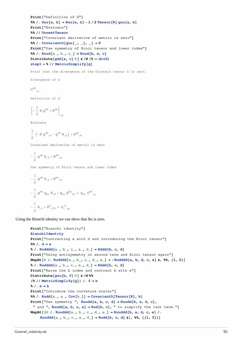
Print@"Covariant derivative of metric is zero"D%% . CovariantD@guu@_, _D, _D ® 0

Print@"Use symmetry of Ricci tensor and lower index"D%% . Ruud@a_, b_, c_D ® Ruud@b, a, cDDistribute@gdd@a, cD ð D & H% divGLstep1 = % MetricSimplify@gDProof that the divergence of the Einstein tensor G is zero.

Divergence of G

Gab;b

Definition of G

-1

2R gab + Rab

;b

Evaluate

1

2I-R g ;b

ab - gab R,bM + R ;bab

Covariant derivative of metric is zero

-1

2gab R,b + R ;b

ab

Use symmetry of Ricci tensor and lower index

-1

2gab R,b + R ;b

ba

-1

2gab gac R,b + gac R ;b

ba gac Gab

;b

-1

2R,c + R c;b

b Gcb;b

Using the Bianchi identity we can show that lhs is zero.

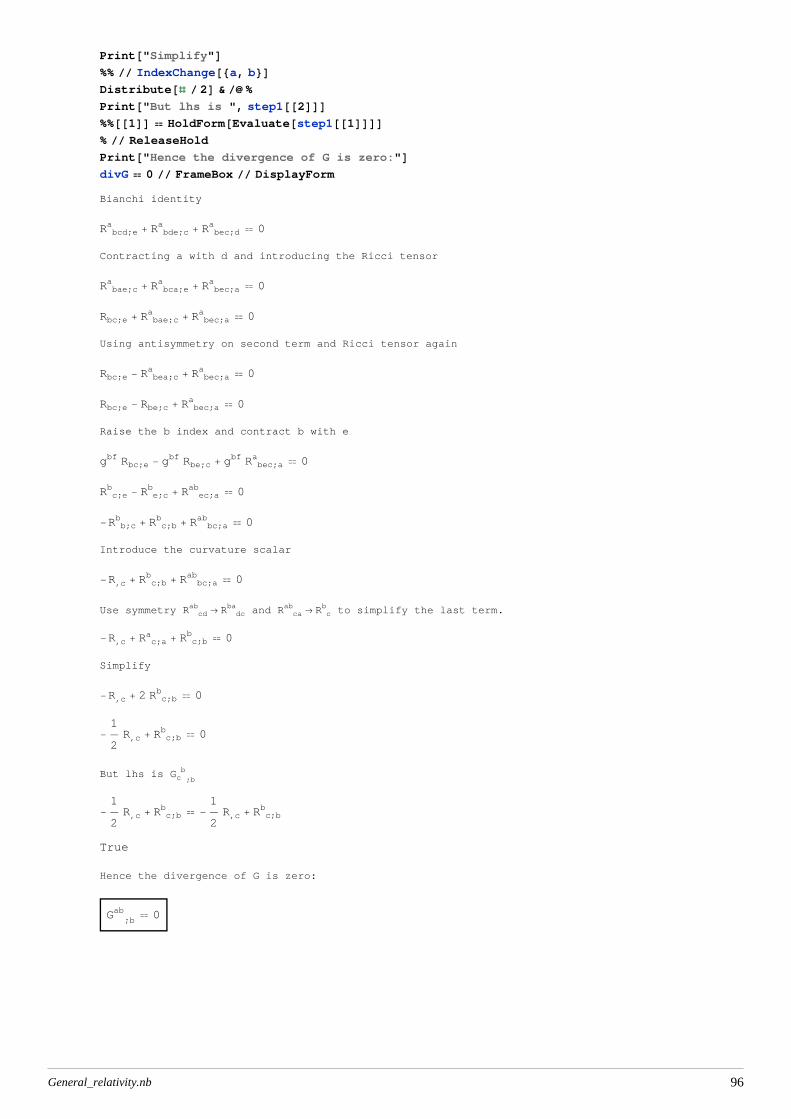
Print@"Bianchi identity"DBianchiIdentity

Print@"Contracting a with d and introducing the Ricci tensor"D%% . d ® a

% . Rudddd@a_, b_, c_, a_, d_D ® Rddd@b, c, dDPrint@"Using antisymmetry on second term and Ricci tensor again"DMapAt@ð . Rudddd@a_, b_, c_, d_, e_D ® -Rudddd@a, b, d, c, eD &, %%, 81, 2<D% . Rudddd@a_, b_, c_, a_, d_D ® Rddd@b, c, dDPrint@"Raise the b index and contract b with e"DDistribute@guu@b, fD ð D & %%H% MetricSimplify@gDL . f ® b

% . e ® b

Print@"Introduce the curvature scalar"D%% . Rudd@a_, a_, Cov@b_DD ® CovariantD@Tensor@RD, bDPrint@"Use symmetry ", Ruudd@a, b, c, dD ® Ruudd@b, a, d, cD," and ", Ruudd@a, b, c, aD ® Rud@b, cD, " to simplify the last term."D

MapAt@Hð . Ruuddd@a_, b_, c_, d_, e_D ® Ruuddd@b, a, d, c, eD .Ruuddd@a_, b_, c_, a_, d_D ® Rudd@b, c, dD &L, %%, 881, 3<<D


Ruuddd@a_, b_, c_, a_, d_D ® Rudd@b, c, dD &L, %%, 881, 3<<DPrint@"Simplify"D%% IndexChange@8a, b<DDistribute@ð 2D & %

Print@"But lhs is ", step1@@2DDD%%@@1DD HoldForm@Evaluate@step1@@1DDDD% ReleaseHold

Print@"Hence the divergence of G is zero:"DdivG 0 FrameBox DisplayForm

Bianchi identity

R bcd;ea + R bde;c

a + R bec;da 0

Contracting a with d and introducing the Ricci tensor

R bae;ca + R bca;e

a + R bec;aa 0

Rbc;e + R bae;ca + R bec;a

a 0

Using antisymmetry on second term and Ricci tensor again

Rbc;e - R bea;ca + R bec;a

a 0

Rbc;e - Rbe;c + R bec;aa 0

Raise the b index and contract b with e

gbf Rbc;e - gbf Rbe;c + gbf R bec;aa 0

R c;eb - R e;c

b + R ec;aab 0

-R b;cb + R c;b

b + R bc;aab 0

Introduce the curvature scalar

-R,c + R c;bb + R bc;a

ab 0

Use symmetry R cdab ® R dc

ba and R caab ® R c

b to simplify the last term.

-R,c + R c;aa + R c;b

b 0

Simplify

-R,c + 2 R c;bb 0

-1

2R,c + R c;b

b 0

But lhs is Gcb;b

-1

2R,c + R c;b

b -1

2R,c + R c;b

b

True

Hence the divergence of G is zero:

Gab;b

0


7) Extras

ã a) For covariant differentiation we can reach inside the derivative and lower the index.

step1 = CovariantD@NestedTensor@gdd@a, dD Τud@d, bDD, cDstep2 = % UnnestTensor

step2 step1

Print@"Covariant derivative of metric tensor is zero"D%% . CovariantD@gdd@_, _D, _D ® 0

Print@"We can lower indices inside a covariant derivative from outside"DMapAt@MetricSimplify@gD, %%, 82, 1<D FrameBox DisplayForm

Igad Τ bd M

;c

gad;c Τ bd + gad Τ b;c

d

gad;c Τ bd + gad Τ b;c

d Igad Τ bd M

;c

Covariant derivative of metric tensor is zero

gad Τ b;cd Igad Τ b

d M;c

We can lower indices inside a covariant derivative from outside

gad Τ b;cd Τab;c

ã b) Covariant differentiation commutator.

? CovariantCommutator

CovariantCommutator@8c1, c2<, R, dD@termD will calculate the covariant

commutator, CovariantD@term,8c1,c2<D - CovariantD@term,8c2,c1<D, and express

the result in terms of the Riemann tensor R. d is the dummy index introduced.

8Λd@aD, Λu@aD, Τuu@a, bD, Τuud@a, b, cD, Λu@aD Λd@bD<CovariantCommutator@8d, e<, R, fD %

9Λa, Λa, Τab, Τ cab , Λa Λb=

9R adef Λf, -R fde

a Λf, -R fdeb Τaf - R fde

a Τfb, R cdef Τ f

ab - R fdeb Τ c

af - R fdea Τ c

fb , -R fdea Λf Λb + R bde

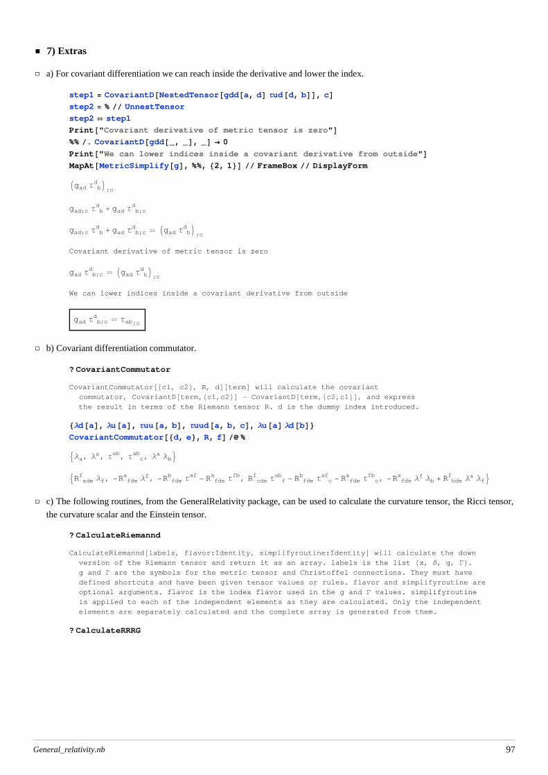
f Λa Λf=ã c) The following routines, from the GeneralRelativity package, can be used to calculate the curvature tensor, the Ricci tensor,

the curvature scalar and the Einstein tensor.

? CalculateRiemannd

CalculateRiemannd@labels, flavor:Identity, simplifyroutine:IdentityD will calculate the down

version of the Riemann tensor and return it as an array. labels is the list 8x, ∆, g, G<.g and G are the symbols for the metric tensor and Christoffel connections. They must have

defined shortcuts and have been given tensor values or rules. flavor and simplifyroutine are

optional arguments. flavor is the index flavor used in the g and G values. simplifyroutine

is applied to each of the independent elements as they are calculated. Only the independent

elements are separately calculated and the complete array is generated from them.

? CalculateRRRG


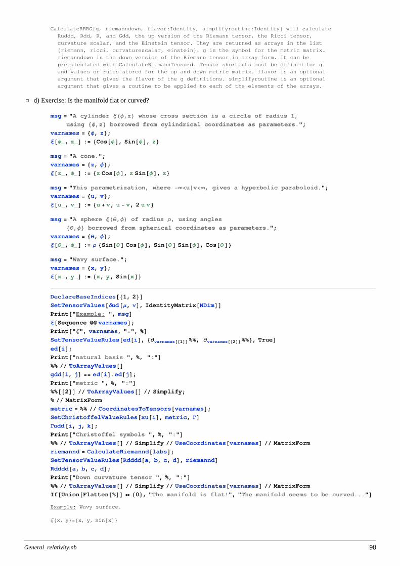
CalculateRRRG@g, riemanndown, flavor:Identity, simplifyroutine:IdentityD will calculate

Ruddd, Rdd, R, and Gdd, the up version of the Riemann tensor, the Ricci tensor,

curvature scalar, and the Einstein tensor. They are returned as arrays in the list8riemann, ricci, curvaturescalar, einstein<. g is the symbol for the metric matrix.

riemanndown is the down version of the Riemann tensor in array form. It can be

precalculated with CalculateRiemannTensord. Tensor shortcuts must be defined for g

and values or rules stored for the up and down metric matrix. flavor is an optional

argument that gives the flavor of the g definitions. simplifyroutine is an optional

argument that gives a routine to be applied to each of the elements of the arrays.

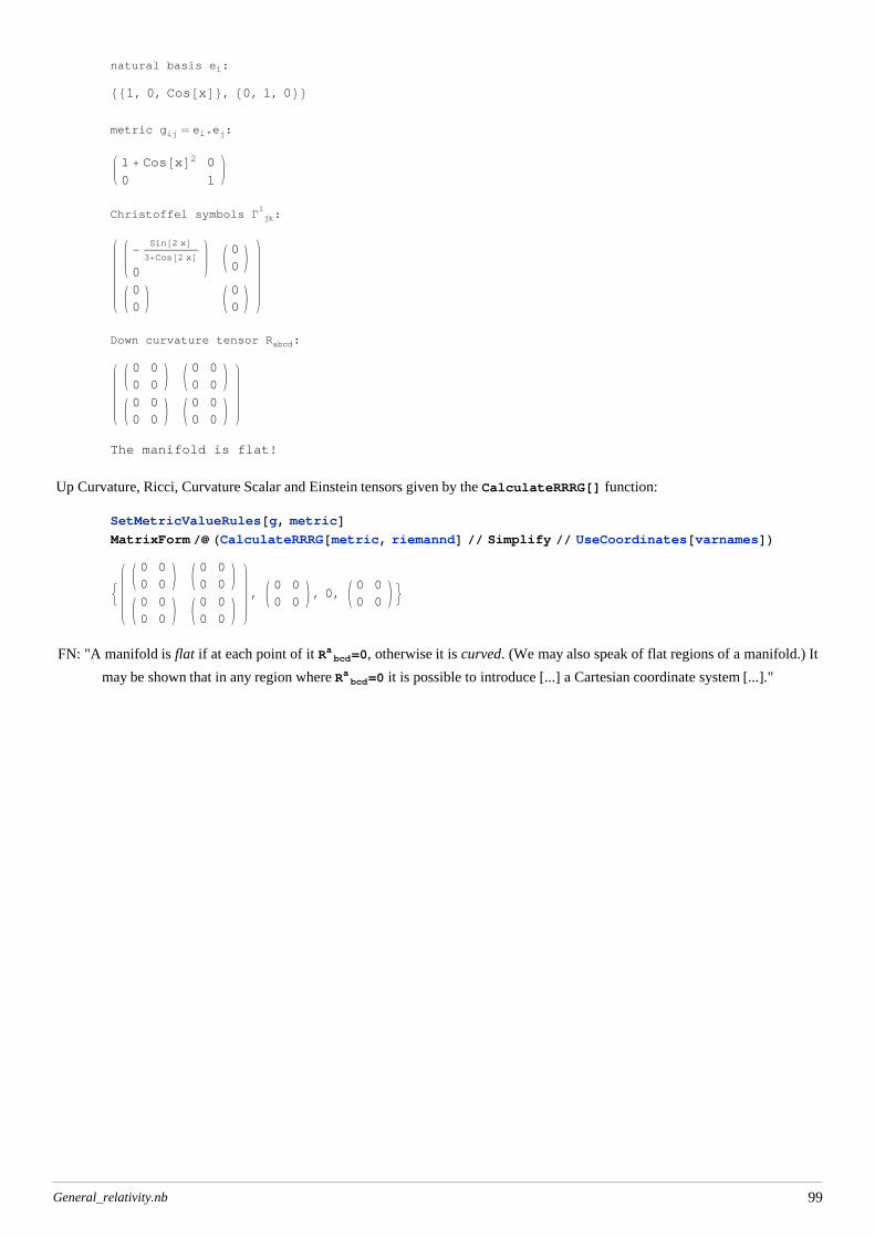
ã d) Exercise: Is the manifold flat or curved?

msg = "A cylinder ΞHΦ,zL whose cross section is a circle of radius 1,

using 8Φ,z< borrowed from cylindrical coordinates as parameters.";

varnames = 8Φ, z<;Ξ@Φ_, z_D := 8Cos@ΦD, Sin@ΦD, z<msg = "A cone.";

varnames = 8z, Φ<;Ξ@z_, Φ_D := 8z Cos@ΦD, z Sin@ΦD, z<msg = "This parametrization, where -¥<uÈv<¥, gives a hyperbolic paraboloid.";

varnames = 8u, v<;Ξ@u_, v_D := 8u + v, u - v, 2 u v<msg = "A sphere ΞHΘ,ΦL of radius Ρ, using angles8Θ,Φ< borrowed from spherical coordinates as parameters.";

varnames = 8Θ, Φ<;Ξ@Θ_, Φ_D := Ρ 8Sin@ΘD Cos@ΦD, Sin@ΘD Sin@ΦD, Cos@ΘD<msg = "Wavy surface.";

varnames = 8x, y<;Ξ@x_, y_D := 8x, y, Sin@xD<DeclareBaseIndices@81, 2<DSetTensorValues@∆ud@Μ, ΝD, IdentityMatrix@NDimDDPrint@"Example: ", msgDΞ@Sequence varnamesD;Print@"Ξ", varnames, "=", %DSetTensorValueRules@ed@iD, 8¶varnames@@1DD %%, ¶varnames@@2DD %%<, TrueDed@iD;Print@"natural basis ", %, ":"D%% ToArrayValues@Dgdd@i, jD == [email protected]@jD;Print@"metric ", %, ":"D%%@@2DD ToArrayValues@D Simplify;

% MatrixForm

metric = %% CoordinatesToTensors@varnamesD;SetChristoffelValueRules@xu@iD, metric, GDGudd@i, j, kD;Print@"Christoffel symbols ", %, ":"D%% ToArrayValues@D Simplify UseCoordinates@varnamesD MatrixForm

riemannd = CalculateRiemannd@labsD;SetTensorValueRules@Rdddd@a, b, c, dD, riemanndDRdddd@a, b, c, dD;Print@"Down curvature tensor ", %, ":"D%% ToArrayValues@D Simplify UseCoordinates@varnamesD MatrixForm

If@Union@Flatten@%DD 80<, "The manifold is flat!", "The manifold seems to be curved..."DExample: Wavy surface.

Ξ8x, y<=8x, y, Sin@xD<


natural basis ei:

881, 0, Cos@xD<, 80, 1, 0<<metric gij ei.ej:

1 + Cos@xD2 0

0 1

Christoffel symbols G jki

:

-Sin@2 xD

3+Cos@2 xD0

K 00

OK 00

O K 00

ODown curvature tensor Rabcd:

K 0 00 0

O K 0 00 0

OK 0 00 0

O K 0 00 0

OThe manifold is flat!

Up Curvature, Ricci, Curvature Scalar and Einstein tensors given by the CalculateRRRG[] function:

SetMetricValueRules@g, metricDMatrixForm HCalculateRRRG@metric, riemanndD Simplify UseCoordinates@varnamesDL: K 0 0

0 0O K 0 0

0 0O

K 0 00 0

O K 0 00 0

O , K 0 00 0

O, 0, K 0 00 0

O>

FN: "A manifold is flat if at each point of it R bcda =0, otherwise it is curved. (We may also speak of flat regions of a manifold.) It

may be shown that in any region where R bcda =0 it is possible to introduce [...] a Cartesian coordinate system [...]."


3.3 Curvature and parallel transport p. 105 - 110


labs = 8x, ∆, g, G<;DeclareBaseIndices@80, 1, 2, 3<DDefineTensorShortcuts@88Λ, Λo, x, xP, Ξ, DΛ, i, j, u<, 1<,88∆, g, f<, 2<,88G, GP<, 3<,88R<, 4<DDeclareTensorSymmetries@G, 3, 81, 82, 3<<DH* - - - *LRiemannToChristoffelRule = LHSSymbolsToPatterns@8a, b, c, d<DRiemannRule;

ChristoffelToRiemannRule = LHSSymbolsToPatterns@8a, b, c, d, e<DReverseRiemannRule;

Format@Integral@expr_DD := DisplayFormARowBoxA9"Ù", RowBox@8"H", expr, "L"<D=EEFormat@ContourIntegral@expr_DD := DisplayFormARowBoxA9"", RowBox@8"H", expr, "L"<D=EE8Integral@"any expression"D, ContourIntegral@"any expression"D<victor@a_, b_, linecolor_: [email protected] := 8

Graphics3D@[email protected], [email protected], Point@aD<D,Graphics3D@8linecolor, Line@8a, a + b<D<D,Graphics3D@[email protected], [email protected], Point@a + bD<D<;

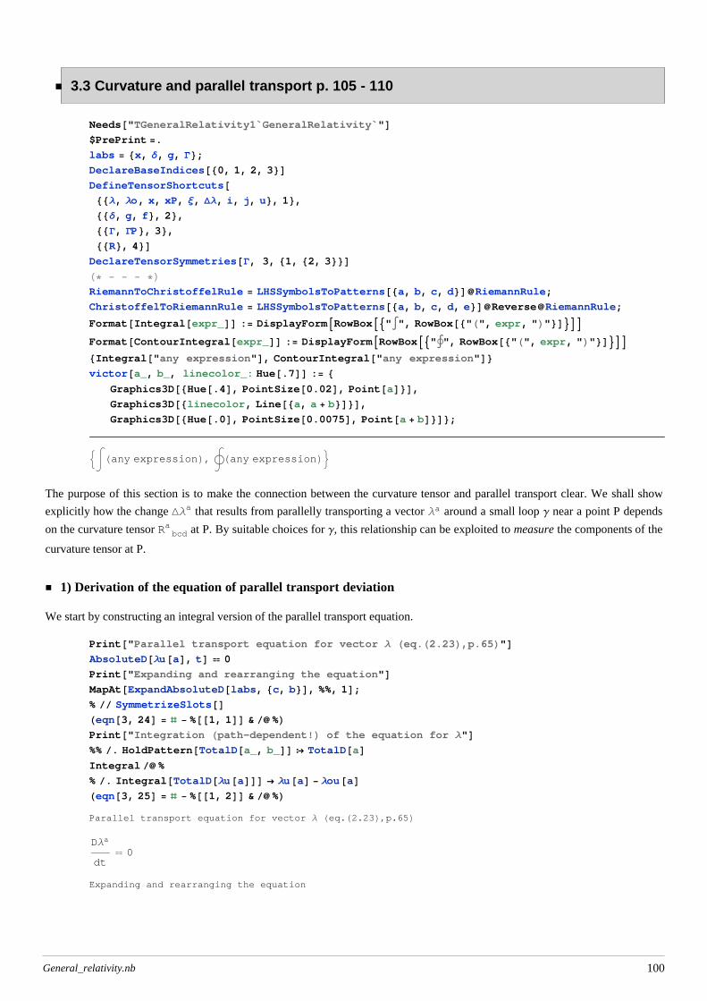
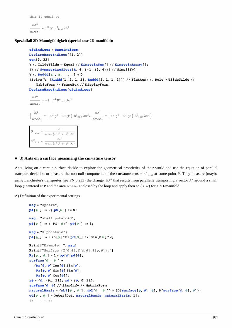
:à Hany expressionL, ¨ Hany expressionL>The purpose of this section is to make the connection between the curvature tensor and parallel transport clear. We shall show

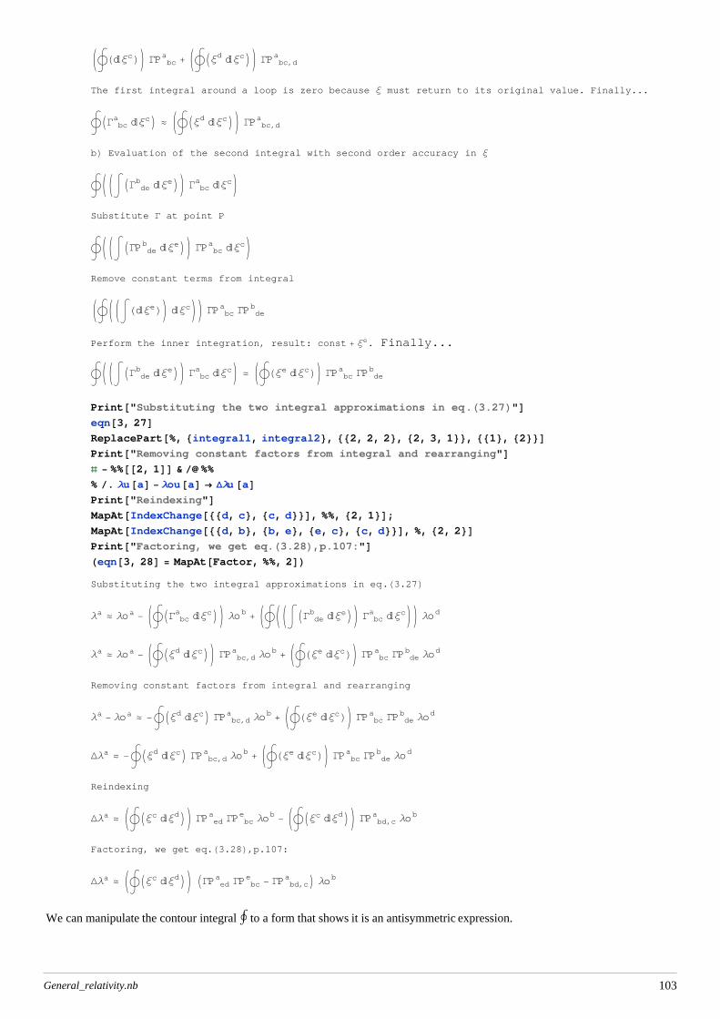
explicitly how the change DΛa that results from parallelly transporting a vector Λa around a small loop Γ near a point P depends

on the curvature tensor R bcda at P. By suitable choices for Γ, this relationship can be exploited to measure the components of the

curvature tensor at P.

1) Derivation of the equation of parallel transport deviation

We start by constructing an integral version of the parallel transport equation.

Print@"Parallel transport equation for vector Λ Heq.H2.23L,p.65L"DAbsoluteD@Λu@aD, tD 0

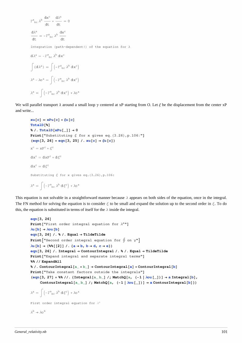
Print@"Expanding and rearranging the equation"DMapAt@ExpandAbsoluteD@labs, 8c, b<D, %%, 1D;% SymmetrizeSlots@DHeqn@3, 24D = ð - %@@1, 1DD & %LPrint@"Integration Hpath–dependent!L of the equation for Λ"D%% . HoldPattern@TotalD@a_, b_DD ¦ TotalD@aDIntegral %

% . Integral@TotalD@Λu@aDDD ® Λu@aD - Λou@aDHeqn@3, 25D = ð - %@@1, 2DD & %LParallel transport equation for vector Λ Heq.H2.23L,p.65LDΛa

dt 0

Expanding and rearranging the equation


G bca Λb

âxc

ât+

âΛa

ât 0

âΛa

ât -G bc

a Λbâxc

ât

Integration Hpath–dependent!L of the equation for Λ

âΛa -G bca Λb âxc

à HâΛaL à I-G bca Λb âxcM

Λa - Λoa à I-G bca Λb âxcM

Λa à I-G bca Λb âxcM + Λoa

We will parallel transport Λ around a small loop Γ centered at xP starting from O. Let Ξ be the displacement from the center xP

and write...

xu@cD xPu@cD + Ξu@cDTotalD@%D% . TotalD@xPu@_DD ® 0

Print@"Substituting Ξ for x gives eq.H3.26L,p.106:"DHeqn@3, 26D = eqn@3, 25D . xu@cD ® Ξu@cDLxc xPc + Ξc

âxc âxPc + âΞc

âxc âΞc

Substituting Ξ for x gives eq.H3.26L,p.106:Λa à I-G bc

a Λb âΞcM + Λoa

This equation is not solvable in a straightforward manner because Λ appears on both sides of the equation, once in the integral.

The FN method for solving the equation is to consider Ξ to be small and expand the solution up to the second order in Ξ. To do

this, the equation is substituted in terms of itself for the Λ inside the integral.

eqn@3, 26DPrint@"First order integral equation for Λa"DΛu@bD ® Λou@bDeqn@3, 26D . % . Equal ® TildeTilde

PrintA"Second order integral equation for on Γ"EΛu@bD ® H%%@@2DD . 8a ® b, b ® d, c ® e<Leqn@3, 26D . Integral ® ContourIntegral . % . Equal ® TildeTilde

Print@"Expand integral and separate integral terms"D%% ExpandAll

% . ContourIntegral@a_ + b_D ® ContourIntegral@aD + ContourIntegral@bDPrint@"Take constant factors outside the integrals"DHeqn@3, 27D = %% . 8Integral@a_ b_D ; MatchQ@a, H-1 Λou@_DLD ® a Integral@bD,

ContourIntegral@a_ b_D ; MatchQ@a, H-1 Λou@_DLD ® a ContourIntegral@bD<LΛa à I-G bc

a Λb âΞcM + Λoa

First order integral equation for Λa

Λb ® Λob


Λa » à I-G bca Λob âΞcM + Λoa

Second order integral equation for on Γ

Λb ® à I-G deb Λod âΞeM + Λob

Λa » ¨ K-G bca Kà I-G de

b Λod âΞeM + ΛobO âΞcO + Λoa

Expand integral and separate integral terms

Λa » ¨ K-à I-G deb Λod âΞeM G bc

a âΞc - G bca Λob âΞcO + Λoa

Λa » ¨ K-à I-G deb Λod âΞeM G bc

a âΞcO + ¨ I-G bca Λob âΞcM + Λoa

Take constant factors outside the integrals

Λa » Λoa - K¨ IG bca âΞcMO Λob + K¨ KKà IG de

b âΞeMO G bca âΞcOO Λod

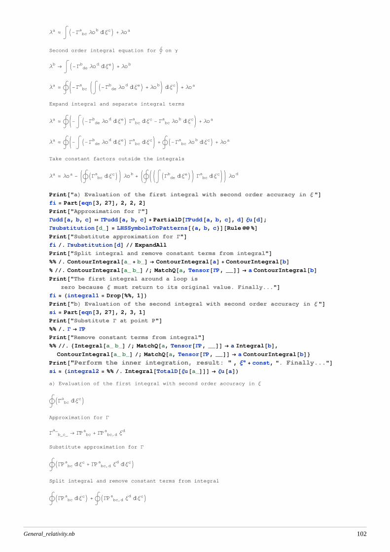
Print@"aL Evaluation of the first integral with second order accuracy in Ξ "Dfi = Part@eqn@3, 27D, 2, 2, 2DPrint@"Approximation for G"DGudd@a, b, cD GPudd@a, b, cD + PartialD@GPudd@a, b, cD, dD Ξu@dD;Gsubstitution@d_D = LHSSymbolsToPatterns@8a, b, c<D@Rule %DPrint@"Substitute approximation for G"Dfi . Gsubstitution@dD ExpandAll

Print@"Split integral and remove constant terms from integral"D%% . ContourIntegral@a_ + b_D ® ContourIntegral@aD + ContourIntegral@bD% . ContourIntegral@a_ b_D ; MatchQ@a, Tensor@GP, __DD ® a ContourIntegral@bDPrint@"The first integral around a loop is

zero because Ξ must return to its original value. Finally..."Dfi » Hintegral1 = Drop@%%, 1DLPrint@"bL Evaluation of the second integral with second order accuracy in Ξ "Dsi = Part@eqn@3, 27D, 2, 3, 1DPrint@"Substitute G at point P"D%% . G ® GP

Print@"Remove constant terms from integral"D%% . 8Integral@a_ b_D ; MatchQ@a, Tensor@GP, __DD ® a Integral@bD,

ContourIntegral@a_ b_D ; MatchQ@a, Tensor@GP, __DD ® a ContourIntegral@bD<Print@"Perform the inner integration, result: " , Ξe + const, ". Finally..."Dsi » Hintegral2 = %% . Integral@TotalD@Ξu@a_DDD ® Ξu@aDLaL Evaluation of the first integral with second order accuracy in Ξ

¨ IG bca âΞcM

Approximation for G

G b_c_a_

® GP bca + GP bc,d

a Ξd

Substitute approximation for G

¨ IGP bca âΞc + GP bc,d

a Ξd âΞcMSplit integral and remove constant terms from integral

¨ IGP bca âΞcM + ¨ IGP bc,d

a Ξd âΞcM


K¨ HâΞcLO GP bca + K¨ IΞd âΞcMO GP bc,d

a

The first integral around a loop is zero because Ξ must return to its original value. Finally...

¨ IG bca âΞcM » K¨ IΞd âΞcMO GP bc,d

a

bL Evaluation of the second integral with second order accuracy in Ξ

¨ KKà IG deb âΞeMO G bc

a âΞcOSubstitute G at point P

¨ KKà IGP deb âΞeMO GP bc

a âΞcORemove constant terms from integral

K¨ KKà HâΞeLO âΞcOO GP bca GP de

b

Perform the inner integration, result: const + Ξe. Finally...

¨ KKà IG deb âΞeMO G bc

a âΞcO » K¨ HΞe âΞcLO GP bca GP de

b

Print@"Substituting the two integral approximations in eq.H3.27L"Deqn@3, 27DReplacePart@%, 8integral1, integral2<, 882, 2, 2<, 82, 3, 1<<, 881<, 82<<DPrint@"Removing constant factors from integral and rearranging"Dð - %%@@2, 1DD & %%

% . Λu@aD - Λou@aD ® DΛu @aDPrint@"Reindexing"DMapAt@IndexChange@88d, c<, 8c, d<<D, %%, 82, 1<D;MapAt@IndexChange@88d, b<, 8b, e<, 8e, c<, 8c, d<<D, %, 82, 2<DPrint@"Factoring, we get eq.H3.28L,p.107:"DHeqn@3, 28D = MapAt@Factor, %%, 2DLSubstituting the two integral approximations in eq.H3.27LΛa » Λoa - K¨ IG bc

a âΞcMO Λob + K¨ KKà IG deb âΞeMO G bc

a âΞcOO Λod

Λa » Λoa - K¨ IΞd âΞcMO GP bc,da Λob + K¨ HΞe âΞcLO GP bc

a GP deb Λod

Removing constant factors from integral and rearranging

Λa - Λoa » -¨ IΞd âΞcM GP bc,da Λob + K¨ HΞe âΞcLO GP bc

a GP deb Λod

DΛa » -¨ IΞd âΞcM GP bc,da Λob + K¨ HΞe âΞcLO GP bc

a GP deb Λod

Reindexing

DΛa » K¨ IΞc âΞdMO GP eda GP bc

e Λob - K¨ IΞc âΞdMO GP bd,ca Λob

Factoring, we get eq.H3.28L,p.107:DΛa » K¨ IΞc âΞdMO IGP ed

a GP bce - GP bd,c

a M Λob

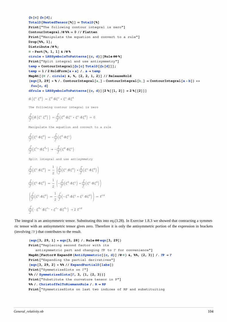
We can manipulate the contour integral to a form that shows it is an antisymmetric expression.


Ξu@cD Ξu@dD;TotalD@NestedTensor@%DD TotalD@%DPrint@"The following contour integral is zero"DContourIntegral %% 0 Flatten

Print@"Manipulate the equation and convert to a rule"DDrop@%%, 1D;Distribute %;

ð - Part@%, 1, 1D & %

cirule = LHSSymbolsToPatterns@8c, d<D@Rule %DPrint@"Split integral and use antisymmetry"Dtemp = ContourIntegral@Ξu@cD TotalD@Ξu@dDDD;temp 1 2 HoldForm@a + aD . a ® temp

MapAt@Hð . ciruleL &, %, 82, 2, 1, 2<D ReleaseHoldHeqn@3, 29D = % . ContourIntegral@a_D - ContourIntegral@b_D ® ContourIntegral@a - bDL ==

fuu@c, dDdfrule = LHSSymbolsToPatterns@8c, d<D@2 %@@1, 2DD ® 2 %@@2DDDâIΞc ΞdM Ξd âΞc + Ξc âΞd

The following contour integral is zero

¨ IâIΞc ΞdMM ¨ IΞd âΞc + Ξc âΞdM 0

Manipulate the equation and convert to a rule

¨ IΞc âΞdM -¨ IΞd âΞcM¨ IΞ

c_âΞ

d_M ® -¨ IΞd âΞcMSplit integral and use antisymmetry

¨ IΞc âΞdM 1

2K¨ IΞc âΞdM + ¨ IΞc âΞdMO

¨ IΞc âΞdM 1

2K-¨ IΞd âΞcM + ¨ IΞc âΞdMO

¨ IΞc âΞdM 1

2¨ I-Ξd âΞc + Ξc âΞdM fcd

¨ I-Ξd_

âΞc_

+ Ξc_

âΞd_M ® 2 fcd

The integral is an antisymmetric tensor. Substituting this into eq.(3.28). In Exercise 1.8.3 we showed that contracting a symmet-

ric tensor with an antisymmetric tensor gives zero. Therefore it is only the antisymmetric portion of the expression in brackets

(involving GP) that contributes to the result.

Heqn@3, 29, 1D = eqn@3, 28D . Rule eqn@3, 29DLPrint@"Replacing second factor with its

antisymmetric part and changing GP to G for convenience"DMapAt@Factor ExpandHAntiSymmetric@8c, d<D ð L &, %%, 82, 3<D . GP ® G

Print@"Expanding the partial derivatives"DHeqn@3, 29, 2D = %% ExpandPartialD@labsDLPrint@"SymmetrizeSlots on G"D%% SymmetrizeSlots@G, 3, 81, 82, 3<<DPrint@"Substitute the curvature tensor in P"D%% . ChristoffelToRiemannRule . R ® RP

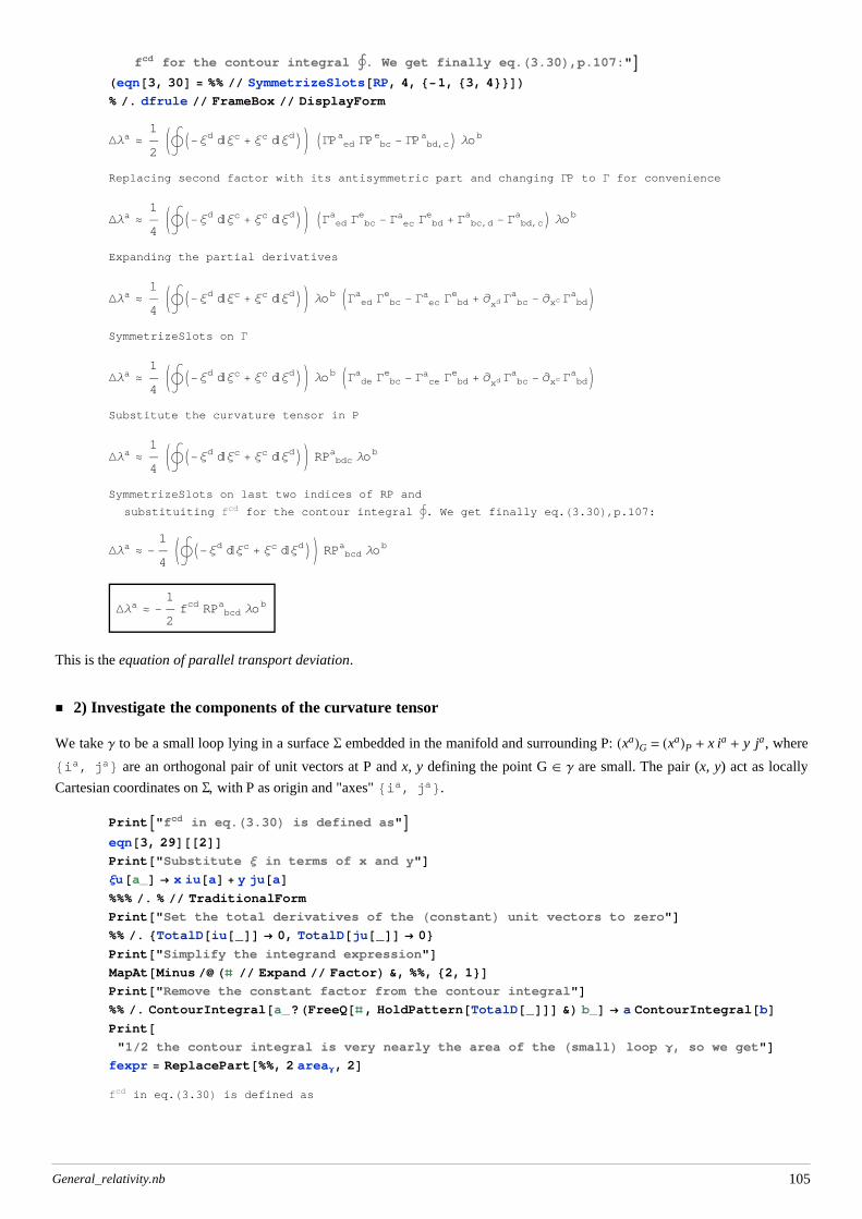
PrintA"SymmetrizeSlots on last two indices of RP and substituiting

fcd for the contour integral . We get finally eq.H3.30L,p.107:"E


PrintA"SymmetrizeSlots on last two indices of RP and substituiting

fcd for the contour integral . We get finally eq.H3.30L,p.107:"EHeqn@3, 30D = %% SymmetrizeSlots@RP, 4, 8-1, 83, 4<<DL% . dfrule FrameBox DisplayForm

DΛa »1

2K¨ I-Ξd âΞc + Ξc âΞdMO IGP ed

a GP bce - GP bd,c

a M Λob

Replacing second factor with its antisymmetric part and changing GP to G for convenience

DΛa »1

4K¨ I-Ξd âΞc + Ξc âΞdMO IG ed

a G bce - G ec

a G bde + G bc,d

a - G bd,ca M Λob

Expanding the partial derivatives

DΛa »1

4K¨ I-Ξd âΞc + Ξc âΞdMO Λob JG ed

a G bce - G ec

a G bde + ¶xd G bc

a - ¶xc G bda N

SymmetrizeSlots on G

DΛa »1

4K¨ I-Ξd âΞc + Ξc âΞdMO Λob JG de

a G bce - G ce

a G bde + ¶xd G bc

a - ¶xc G bda N

Substitute the curvature tensor in P

DΛa »1

4K¨ I-Ξd âΞc + Ξc âΞdMO RP bdc

a Λob

SymmetrizeSlots on last two indices of RP and

substituiting fcd for the contour integral . We get finally eq.H3.30L,p.107:DΛa » -

1

4K¨ I-Ξd âΞc + Ξc âΞdMO RP bcd

a Λob

DΛa » -1

2fcd RP bcd

a Λob

This is the equation of parallel transport deviation.

2) Investigate the components of the curvature tensor

We take Γ to be a small loop lying in a surface S embedded in the manifold and surrounding P: HxaLG = HxaLP + x ia + y ja, where8ia, ja< are an orthogonal pair of unit vectors at P and x, y defining the point G Î Γ are small. The pair (x, y) act as locally

Cartesian coordinates on S, with P as origin and "axes" 8ia, ja<.

PrintA"fcd in eq.H3.30L is defined as"Eeqn@3, 29D@@2DDPrint@"Substitute Ξ in terms of x and y"DΞu@a_D ® x iu@aD + y ju@aD%%% . % TraditionalForm

Print@"Set the total derivatives of the HconstantL unit vectors to zero"D%% . 8TotalD@iu@_DD ® 0, TotalD@ju@_DD ® 0<Print@"Simplify the integrand expression"DMapAt@Minus Hð Expand FactorL &, %%, 82, 1<DPrint@"Remove the constant factor from the contour integral"D%% . ContourIntegral@a_?HFreeQ@ð, HoldPattern@TotalD@_DDD &L b_D ® a ContourIntegral@bDPrint@"12 the contour integral is very nearly the area of the HsmallL loop Γ, so we get"D

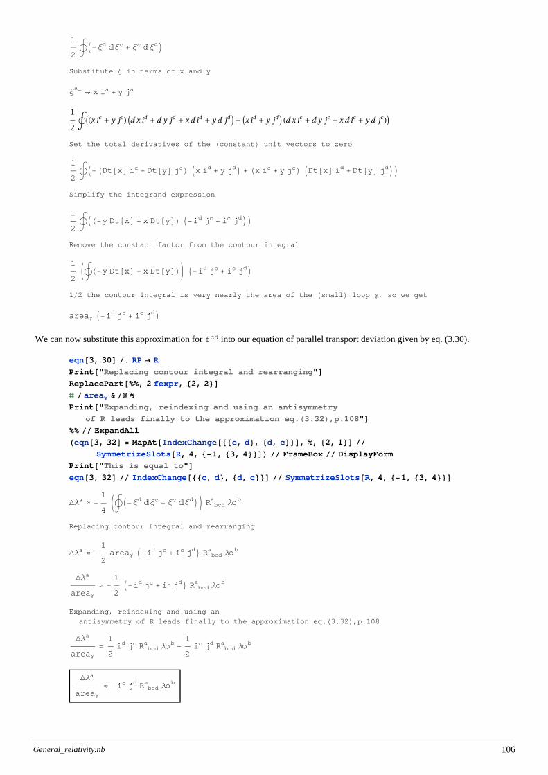
fexpr = ReplacePart@%%, 2 areaΓ, 2Dfcd in eq.H3.30L is defined as


1

2¨ I-Ξd âΞc + Ξc âΞdM

Substitute Ξ in terms of x and y

Ξa_

® x ia + y ja

1

2¨ IHx ic + y jcL Iâ x id + â y jd + x â id + y â jd M - Ix id + y jd M Hâ x ic + â y jc + x â ic + y â jcLM

Set the total derivatives of the HconstantL unit vectors to zero

1

2¨ I-HDt@xD ic + Dt@yD jcL Ix id + y jdM + Hx ic + y jcL IDt@xD id + Dt@yD jdMM

Simplify the integrand expression

1

2¨ IH-y Dt@xD + x Dt@yDL I-id jc + ic jdMM

Remove the constant factor from the contour integral

1

2K¨ H-y Dt@xD + x Dt@yDLO I-id jc + ic jdM

12 the contour integral is very nearly the area of the HsmallL loop Γ, so we get

areaΓ I-id jc + ic jdMWe can now substitute this approximation for fcd into our equation of parallel transport deviation given by eq. (3.30).

eqn@3, 30D . RP ® R

Print@"Replacing contour integral and rearranging"DReplacePart@%%, 2 fexpr, 82, 2<Dð areaΓ & %

Print@"Expanding, reindexing and using an antisymmetry

of R leads finally to the approximation eq.H3.32L,p.108"D%% ExpandAllHeqn@3, 32D = MapAt@IndexChange@88c, d<, 8d, c<<D, %, 82, 1<D

SymmetrizeSlots@R, 4, 8-1, 83, 4<<DL FrameBox DisplayForm

Print@"This is equal to"Deqn@3, 32D IndexChange@88c, d<, 8d, c<<D SymmetrizeSlots@R, 4, 8-1, 83, 4<<DDΛa » -

1

4K¨ I-Ξd âΞc + Ξc âΞdMO R bcd

a Λob

Replacing contour integral and rearranging

DΛa » -1

2areaΓ I-id jc + ic jdM R bcd

a Λob

DΛa

areaΓ

» -1

2I-id jc + ic jdM R bcd

a Λob

Expanding, reindexing and using an

antisymmetry of R leads finally to the approximation eq.H3.32L,p.108DΛa

areaΓ

»1

2id jc R bcd

a Λob -1

2ic jd R bcd

a Λob

DΛa

areaΓ

» -ic jd R bcda Λob


This is equal to

DΛa

areaΓ

» id jc R bcda Λob

Spezialfall 2D-Mannigfaltigkeit (special case 2D-manifold):

oldindices = BaseIndices;

DeclareBaseIndices@81, 2<Deqn@3, 32D% . TildeTilde ® Equal EinsteinSum@D EinsteinArray@D;H% SymmetrizeSlots@R, 4, 8-1, 83, 4<<D SimplifyL;% . Ruddd@a_, a_, _, _D ® 0HSolve@%, 8Ruddd@1, 2, 1, 2D, Ruddd@2, 1, 1, 2D<D FlattenL . Rule ® TildeTilde

TableForm FrameBox DisplayForm

DeclareBaseIndices@oldindicesDDΛa

areaΓ

» -ic jd R bcda Λob

: DΛ1

areaΓ

Ii2 j1 - i1 j2M R 2121 Λo2,

DΛ2

areaΓ

Ii2 j1 - i1 j2M R 1122 Λo1>

R 2121 »

DΛ1

areaΓ Ii2 j1-i1 j2M Λo2

R 1122 »

DΛ2

areaΓ Ii2 j1-i1 j2M Λo1

3) Ants on a surface measuring the curvature tensor

Ants living on a certain surface decide to explore the geometrical proprieties of their world and use the equation of parallel

transport deviation to measure the non-null components of the curvature tensor R bcda at some point P. They measure (maybe

using Lanchester's transporter, see FN p.233) the change DΛa that results from parallelly transporting a vector Λa around a small

loop Γ centered at P and the area areaΓ enclosed by the loop and apply then eq.(3.32) for a 2D-manifold.

A) Definition of the experimental settings.

msg = "sphere";

pΦ@Φ_D := 0; pΘ@Θ_D := 0;

msg = "shell potatoid";

pΦ@Φ_D := H-Pi - ΦL2; pΘ@Θ_D := 1;

msg = "X potatoid";

pΦ@Φ_D := Sin@ΦD^2; pΘ@Θ_D := Sin@2 ΘD^2;Print@"Example: ", msgDPrint@"Surface 8X@Φ,ΘD,Y@Φ,ΘD,Z@Φ,ΘD<:"DRr@Φ_, Θ_D = 1 + pΦ@ΦD pΘ@ΘD;surface@Φ_, Θ_D =8Rr@Φ, ΘD Cos@ΦD Sin@ΘD,

Rr@Φ, ΘD Sin@ΦD Sin@ΘD,Rr@Φ, ΘD Cos@ΘD<;

rΦ = 8Φ, -Pi, Pi<; rΘ = 8Θ, 0, Pi<;surface@Φ, ΘD Simplify MatrixForm

naturalBasis = 8nb1@Φ_, Θ_D, nb2@Φ_, Θ_D< = 8D@surface@Φ, ΘD, ΦD, D@surface@Φ, ΘD, ΘD<;gd@Φ_, Θ_D = Outer@Dot, naturalBasis, naturalBasis, 1D;H* - - - *L


H* - - - *LPrint@"Chosen point P:"DΦp = 1.5; Θp = 1.0;

p = surface@Φp, ΘpDPrint@"Chosen orthonormal vector pair 8i,j< at P Hnatural basis and 3D-basisL:"DClear@iu1, iu2, ju1, ju2DSolve@8iu1 0.5,8iu1, iu2<.gd@Φp, ΘpD.8iu1, iu2< 1,8ju1, ju2<.gd@Φp, ΘpD.8ju1, ju2< 1,8iu1, iu2<.gd@Φp, ΘpD.8ju1, ju2< 0<D;%@@1DD . Rule ® Set;

ColumnForm 88iu1, iu2<, 8ju1, ju2<<8i, j< = 8iu1 nb1@Φp, ΘpD +

iu2 nb2@Φp, ΘpD, ju1 nb1@Φp, ΘpD +

ju2 nb2@Φp, ΘpD<;ColumnForm %

Print@"Check orthonormality: i.i,j.j and i.j"D8i.i, j.j, i.j< Chop

Print@"Loop Γ:"DΕ = 0.1;

xx@t_D := Ε Cos@tD; yy@t_D := Ε Sin@tD;xG1@t_D := Φp + xx@tD iu1 + yy@tD ju1

xG2@t_D := Θp + xx@tD iu2 + yy@tD ju2

"8ΦHtL,ΘHtL<" == 8xG1@tD, xG2@tD<Print@"Parallel transported vector Λ Hnatural basisL:"D8Λo1, Λo2< = 81, 1<Example: X potatoid

Surface 8X@Φ,ΘD,Y@Φ,ΘD,Z@Φ,ΘD<:Cos@ΦD Sin@ΘD I1 + Sin@2 ΘD2 Sin@ΦD2MSin@ΘD Sin@ΦD I1 + Sin@2 ΘD2 Sin@ΦD2MCos@ΘD I1 + Sin@2 ΘD2 Sin@ΦD2M

Chosen point P:

80.108492, 1.52989, 0.984801<Chosen orthonormal vector pair 8i,j< at P Hnatural basis and 3D-basisL:: 0.5

-0.255063, -0.416714

-0.337998>

: -0.7563780.1750850.630268

, 0.6413870.009216590.767162

>

Check orthonormality: i.i,j.j and i.j

81., 1., 0<Loop Γ:

8ΦHtL,ΘHtL< 81.5 + 0.05 Cos@tD - 0.0416714 Sin@tD, 1. - 0.0255063 Cos@tD - 0.0337998 Sin@tD<Parallel transported vector Λ Hnatural basisL:81, 1<pp = 40;

Potatoid = ParametricPlot3D@surface@Φ, ΘD, Evaluate@rΦD,Evaluate@rΘD, PlotPoints ® 8pp, pp<, DisplayFunction ® IdentityD;

CLΦp = ParametricPlot3D@surface@Φp, ΘD, Evaluate@rΘD, DisplayFunction ® IdentityD;


CLΦp = ParametricPlot3D@surface@Φp, ΘD, Evaluate@rΘD, DisplayFunction ® IdentityD;CLΘp = ParametricPlot3D@surface@Φ, ΘpD, Evaluate@rΦD, DisplayFunction ® IdentityD;nb1p = victor@p, nb1@Φp, ΘpDD;nb2p = victor@p, nb2@Φp, ΘpDD;ip = victor@p, i, [email protected];jp = victor@p, j, [email protected];Γp = ParametricPlot3D@surface@xG1@tD, xG2@tDD, 8t, 0, 2 Π<, DisplayFunction ® IdentityD;g1 = Show@Graphics3D@EdgeForm@D, Axes ® True,

AxesLabel ® 8"X", "Y", "Z"<, ViewPoint ® p + 10 81, 1, 1<D,Potatoid,

Graphics3D@[email protected], Point@pD<D,CLΦp, CLΘp, nb1p, nb2p, ip, jp, Γp, DisplayFunction ® IdentityD;

g2 = ParametricPlot@8xG1@tD, xG2@tD<, 8t, 0, 2 Π - .3<, AspectRatio ® Automatic,

AxesLabel ® 8"ΦΓHtL", "ΘΓHtL"<, DisplayFunction ® IdentityD;Show@GraphicsArray@8g1, g2<D, ImageSize ® 72 ´ 7D;

-1

0

1X

-1

0

1

Y

-1

0

1

Z

-1

0

1X

-1

0

1

Y

1.44 1.46 1.48 1.52 1.54 1.56ΦΓHtL

0.96

0.98

1.02

1.04

ΘΓHtL

ø Plot of ant's world with coordinate lines and natural basis at point P, orthonormal vector pair i , j and loop Γ. ø

B) Theoretically expected results.

DeclareBaseIndices@81, 2<Dmetric = gd@Φ, ΘD CoordinatesToTensors@8Φ, Θ<, uD;SetMetricValueRules@g, metricD; SetChristoffelValueRules@uu@kD, metric, GD;Print@"Vector parallel transport equation on loop Γ"DMapAt@ExpandAbsoluteD@labs, 8c, b<D, AbsoluteD@Λu@aD, tD 0, 1D SymmetrizeSlots@D% EinsteinSum@D ArrayExpansion@aD ToArrayValues@D;% UseCoordinates@8xG1@tD, xG2@tD<, uD;% UseCoordinates@8Λ1@tD, Λ2@tD<, ΛD;% UseCoordinates@8xG1@tD, xG2@tD<, xD;VectorParallelTransportEquationOnΓ = %;

Short@%, 5DRuddd@a, b, c, dD% . RiemannToChristoffelRule8Ruddd@1, 2, 1, 2D, Ruddd@2, 1, 1, 2D<% . RiemannToChristoffelRule

Rtheor = % EinsteinSum@D ToArrayValues@D UseCoordinates@8Φ, Θ<, uD UseCoordinates@8Φ, Θ<, xD;

Rtheorp = 8"Theory", Rtheor . 8Φ ® Φp, Θ ® Θp<<Vector parallel transport equation on loop Γ


G bca Λb

âxc

ât+

âΛa

ât 0

:12

H-0.0337998 Cos@tD + 0.0255063 Sin@tDL524288 5 H1L

H1L2 H1L + H64 H-306 + 16 + 4 1L 1 H4 + 1LL IH1L2 H1LM Λ1@tD + 3 + Λ1 ¢@tD 0, 1 0>

R bcda

-G dea G bc

e + G cea G bd

e - ¶xd G bca + ¶xc G bd

a

9R 2121 , R 112

2 =:-G 2e

1 G 21e + G 1e

1 G 22e - ¶x2 G 21

1 + ¶x1 G 221 , -G 2e

2 G 11e + G 1e

2 G 12e - ¶x2 G 11

2 + ¶x1 G 122 >

8Theory, 88.65686, -3.6638<<C) Ant's experimental results and comparison with theory.

Print@"Measured areaΓ"DareaΓ = 1 2 NIntegrate@xx@tD yy'@tD - yy@tD xx'@tD, 8t, 0, 2 Π<DPrint@"Measured deviation 8DΛ1 ,DΛ2 <"DNDSolve@Union@VectorParallelTransportEquationOnΓ, 8Λ1@0D Λo1, Λ2@0D Λo2<D,8Λ1, Λ2<, 8t, 0, 2 Π<D;8Λ1@2 ΠD, Λ2@2 ΠD< . %;8DΛ1 , DΛ2 < = H% FirstL - 8Λo1, Λo2<8Ruddd@1, 2, 1, 2D, Ruddd@2, 1, 1, 2D<8"Experiment",8R1212 = DΛ1 HareaΓ Λo2 H iu2 ju1 - iu1 ju2LL, R2112 = DΛ2 HareaΓ Λo1 H iu2 ju1 - iu1 ju2LL<<Rtheorp8"Relativ error", 8R1212 %@@2, 1DD - 1, R2112 %@@2, 2DD - 1< * 100 "%"<Measured areaΓ

0.0314159

Measured deviation 8DΛ1,DΛ2<80.0713319, -0.0330282<9R 212

1 , R 1122 =

8Experiment, 88.24799, -3.81899<<8Theory, 88.65686, -3.6638<<8Relativ error, 8-4.72305 %, 4.23566 %<<

"Ants are small and silent. And gigantically mysterious..."


3.4 Geodesic deviation p. 110 - 112


labs = 8x, ∆, g, G<;DeclareBaseIndices@80, 1, 2, 3<DDefineTensorShortcuts@88x, xp, v, vp, Ξ, zero<, 1<,88∆, g<, 2<,88G, Gp<, 3<,88R<, 4<DDeclareZeroTensor@zeroDDeclareTensorSymmetries@G, 3, 81, 82, 3<<DH* - - - *LChristoffelToRiemannRule = LHSSymbolsToPatterns@8a, b, c, d, e<DReverseRiemannRule;

We derive here the equation of geodesic deviation.

Print@"Let there be two affinely parametrized nearby geodesics."DAbsoluteD@vpu@aD, uD 0

MapAt@ExpandAbsoluteD@8xp, ∆, g, Gp<, 8b, c<D, %, 1DHeqn@3, 33D = % . vpu@a_D ® TotalD@xpu@aD, uDL FrameBox DisplayForm

AbsoluteD@vu@aD, uD 0

MapAt@ExpandAbsoluteD@8x, ∆, g, G<, 8b, c<D, %, 1DHeqn@3, 34D = % . vu@a_D ® TotalD@xu@aD, uDL FrameBox DisplayForm

Print@"HWe are going to need the last equation in the form of a rule...L"Dgeodesicrule@b_, c_D =

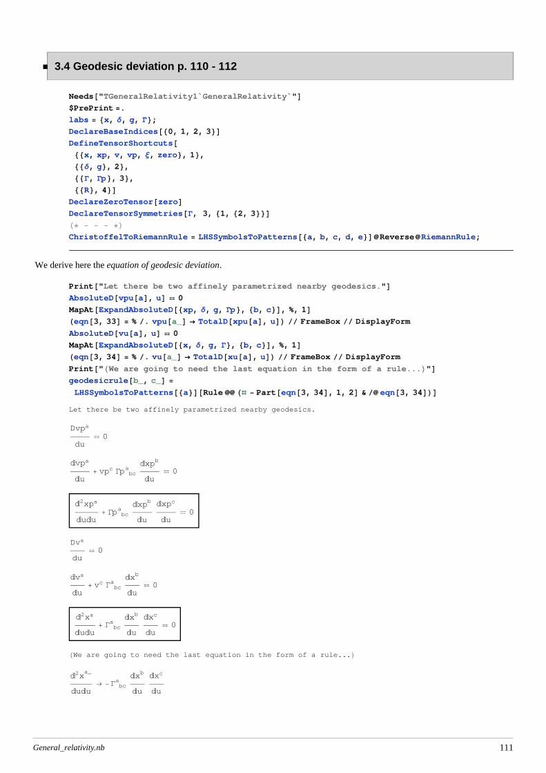
LHSSymbolsToPatterns@8a<D@Rule Hð - Part@eqn@3, 34D, 1, 2D & eqn@3, 34DLDLet there be two affinely parametrized nearby geodesics.

Dvpa

du 0

âvpa

âu+ vpc Gp bc

aâxpb

âu 0

â2xpa

âuâu+ Gp bc

aâxpb

âu

âxpc

âu 0

Dva

du 0

âva

âu+ vc G bc

aâxb

âu 0

â2xa

âuâu+ G bc

aâxb

âu

âxc

âu 0

HWe are going to need the last equation in the form of a rule...Lâ2x

a_

âuâu® -G bc

aâxb

âu

âxc

âu


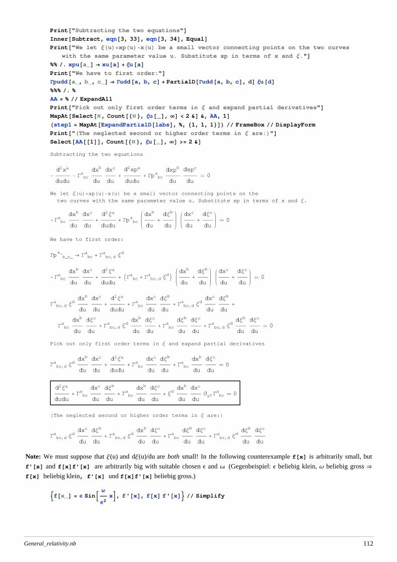
Print@"Subtracting the two equations"DInner@Subtract, eqn@3, 33D, eqn@3, 34D, EqualDPrint@"We let ΞHuL=xpHuL-xHuL be a small vector connecting points on the two curves

with the same parameter value u. Substitute xp in terms of x and Ξ."D%% . xpu@a_D ® xu@aD + Ξu@aDPrint@"We have to first order:"DGpudd@a_, b_, c_D ® Gudd@a, b, cD + PartialD@Gudd@a, b, cD, dD Ξu@dD%%% . %

AA = % ExpandAll

Print@"Pick out only first order terms in Ξ and expand partial derivatives"DMapAt@Select@ð, Count@8ð <, Ξu@_D, ¥D < 2 &D &, AA, 1DHstep1 = MapAt@ExpandPartialD@labsD, %, 81, 1, 1<DL FrameBox DisplayForm

Print@"HThe neglected second or higher order terms in Ξ are:L"DSelect@AA@@1DD, Count@8ð <, Ξu@_D, ¥D >= 2 &DSubtracting the two equations

-â2xa

âuâu- G bc

aâxb

âu

âxc

âu+

â2xpa

âuâu+ Gp bc

aâxpb

âu

âxpc

âu 0

We let ΞHuL=xpHuL-xHuL be a small vector connecting points on the

two curves with the same parameter value u. Substitute xp in terms of x and Ξ.

-G bca

âxb

âu

âxc

âu+

â2Ξa

âuâu+ Gp bc

aâxb

âu+

âΞb

âu

âxc

âu+

âΞc

âu 0

We have to first order:

Gp b_c_a_

® G bca + G bc,d

a Ξd

-G bca

âxb

âu

âxc

âu+

â2Ξa

âuâu+ IG bc

a + G bc,da ΞdM âxb

âu+

âΞb

âu

âxc

âu+

âΞc

âu 0

G bc,da Ξd

âxb

âu

âxc

âu+

â2Ξa

âuâu+ G bc

aâxc

âu

âΞb

âu+ G bc,d

a Ξdâxc

âu

âΞb

âu+

G bca

âxb

âu

âΞc

âu+ G bc,d

a Ξdâxb

âu

âΞc

âu+ G bc

aâΞb

âu

âΞc

âu+ G bc,d

a ΞdâΞb

âu

âΞc

âu 0

Pick out only first order terms in Ξ and expand partial derivatives

G bc,da Ξd

âxb

âu

âxc

âu+

â2Ξa

âuâu+ G bc

aâxc

âu

âΞb

âu+ G bc

aâxb

âu

âΞc

âu 0

â2Ξa

âuâu+ G bc

aâxc

âu

âΞb

âu+ G bc

aâxb

âu

âΞc

âu+ Ξd

âxb

âu

âxc

âu¶xd G bc

a 0

HThe neglected second or higher order terms in Ξ are:LG bc,da Ξd

âxc

âu

âΞb

âu+ G bc,d

a Ξdâxb

âu

âΞc

âu+ G bc

aâΞb

âu

âΞc

âu+ G bc,d

a ΞdâΞb

âu

âΞc

âu

Note: We must suppose that Ξ(u) and dΞ(u)/du are both small! In the following counterexample f[x] is arbitrarily small, but

f'[x] and f[x]f'[x] are arbitrarily big with suitable chosen Ε and Ω. (Gegenbeispiel: Ε beliebig klein, Ω beliebig gross Þ

f[x] beliebig klein, f'[x] und f[x]f'[x] beliebig gross.)

:f@x_D = Ε SinB Ω

Ε2xF, f'@xD, f@xD f'@xD> Simplify


:Ε SinBx Ω

Ε2F, Ω CosB x Ω

Ε2F

Ε,1

2Ω SinB 2 x Ω

Ε2F>

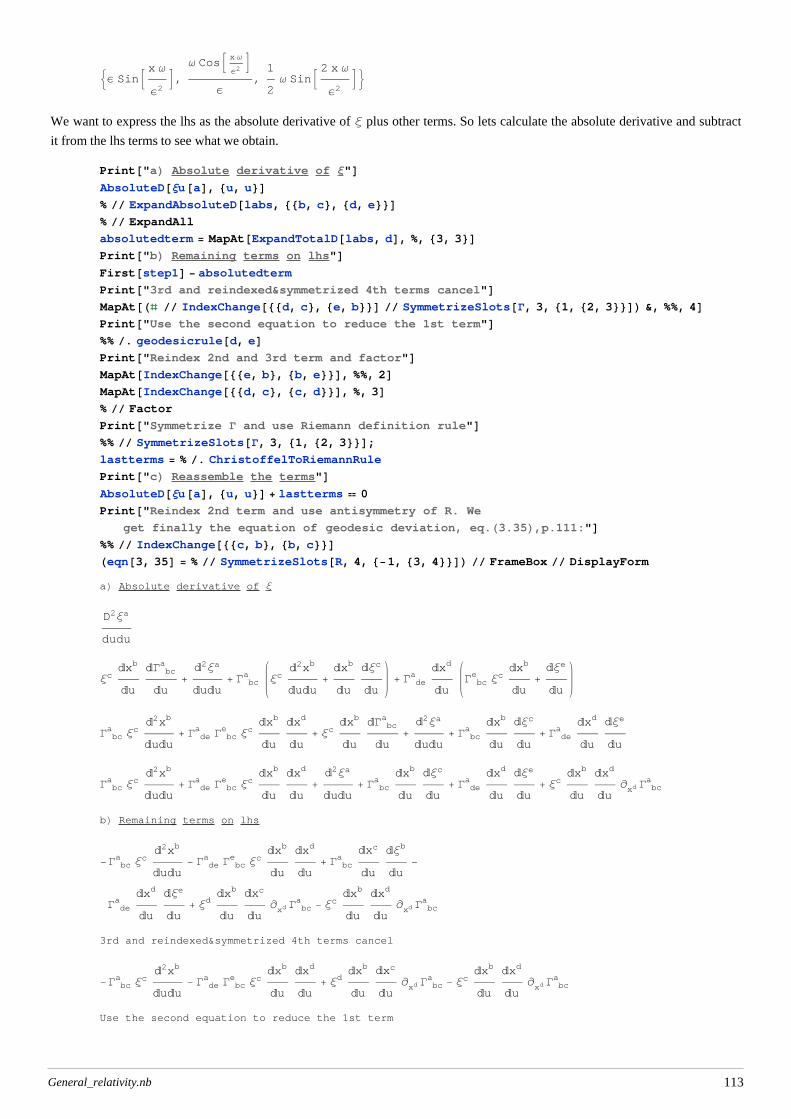
We want to express the lhs as the absolute derivative of Ξ plus other terms. So lets calculate the absolute derivative and subtract

it from the lhs terms to see what we obtain.

Print@"aL Absolute derivative of Ξ"DAbsoluteD@Ξu@aD, 8u, u<D% ExpandAbsoluteD@labs, 88b, c<, 8d, e<<D% ExpandAll

absolutedterm = MapAt@ExpandTotalD@labs, dD, %, 83, 3<DPrint@"bL Remaining terms on lhs"DFirst@step1D - absolutedterm

Print@"3rd and reindexed&symmetrized 4th terms cancel"DMapAt@Hð IndexChange@88d, c<, 8e, b<<D SymmetrizeSlots@G, 3, 81, 82, 3<<DL &, %%, 4DPrint@"Use the second equation to reduce the 1st term"D%% . geodesicrule@d, eDPrint@"Reindex 2nd and 3rd term and factor"DMapAt@IndexChange@88e, b<, 8b, e<<D, %%, 2DMapAt@IndexChange@88d, c<, 8c, d<<D, %, 3D% Factor

Print@"Symmetrize G and use Riemann definition rule"D%% SymmetrizeSlots@G, 3, 81, 82, 3<<D;lastterms = % . ChristoffelToRiemannRule

Print@"cL Reassemble the terms"DAbsoluteD@Ξu@aD, 8u, u<D + lastterms 0

Print@"Reindex 2nd term and use antisymmetry of R. We

get finally the equation of geodesic deviation, eq.H3.35L,p.111:"D%% IndexChange@88c, b<, 8b, c<<DHeqn@3, 35D = % SymmetrizeSlots@R, 4, 8-1, 83, 4<<DL FrameBox DisplayForm

aL Absolute derivative of Ξ

D2Ξa

dudu

Ξcâxb

âu

âG bca

âu+

â2Ξa

âuâu+ G bc

a Ξcâ2xb

âuâu+

âxb

âu

âΞc

âu+ G de

aâxd

âuG bce Ξc

âxb

âu+

âΞe

âu

G bca Ξc

â2xb

âuâu+ G de

a G bce Ξc

âxb

âu

âxd

âu+ Ξc

âxb

âu

âG bca

âu+

â2Ξa

âuâu+ G bc

aâxb

âu

âΞc

âu+ G de

aâxd

âu

âΞe

âu

G bca Ξc

â2xb

âuâu+ G de

a G bce Ξc

âxb

âu

âxd

âu+

â2Ξa

âuâu+ G bc

aâxb

âu

âΞc

âu+ G de

aâxd

âu

âΞe

âu+ Ξc

âxb

âu

âxd

âu¶xd G bc

a

bL Remaining terms on lhs

-G bca Ξc

â2xb

âuâu- G de

a G bce Ξc

âxb

âu

âxd

âu+ G bc

aâxc

âu

âΞb

âu-

G dea

âxd

âu

âΞe

âu+ Ξd

âxb

âu

âxc

âu¶xd G bc

a - Ξcâxb

âu

âxd

âu¶xd G bc

a

3rd and reindexed&symmetrized 4th terms cancel

-G bca Ξc

â2xb

âuâu- G de

a G bce Ξc

âxb

âu

âxd

âu+ Ξd

âxb

âu

âxc

âu¶xd G bc

a - Ξcâxb

âu

âxd

âu¶xd G bc

a

Use the second equation to reduce the 1st term


-G dea G bc

e Ξcâxb

âu

âxd

âu+ G bc

a G deb Ξc

âxd

âu

âxe

âu+ Ξd

âxb

âu

âxc

âu¶xd G bc

a - Ξcâxb

âu

âxd

âu¶xd G bc

a

Reindex 2nd and 3rd term and factor

-G dea G bc

e Ξcâxb

âu

âxd

âu+ G ec

a G dbe Ξc

âxb

âu

âxd

âu+ Ξd

âxb

âu

âxc

âu¶xd G bc

a - Ξcâxb

âu

âxd

âu¶xd G bc

a

-G dea G bc

e Ξcâxb

âu

âxd

âu+ G ec

a G dbe Ξc

âxb

âu

âxd

âu- Ξc

âxb

âu

âxd

âu¶xd G bc

a + Ξcâxb

âu

âxd

âu¶xc G bd

a

-Ξcâxb

âu

âxd

âuJG de

a G bce - G ec

a G dbe + ¶xd G bc

a - ¶xc G bda N

Symmetrize G and use Riemann definition rule

-R bdca Ξc

âxb

âu

âxd

âu

cL Reassemble the terms

D2Ξa

dudu- R bdc

a Ξcâxb

âu

âxd

âu 0

Reindex 2nd term and use antisymmetry of R. We

get finally the equation of geodesic deviation, eq.H3.35L,p.111:D2Ξa

dudu- R cdb

a Ξbâxc

âu

âxd

âu 0

D2Ξa

dudu+ R cbd

a Ξbâxc

âu

âxd

âu 0

Spezialfall 2D-Mannigfaltigkeit (special case 2D-manifold):


DeclareBaseIndices@81, 2<Deqn@3, 35D@@1DD zerou@aD% EinsteinSum@D EinsteinArray@D;% . Ruddd@a_, a_, _, _D ® 0;

% SymmetrizeSlots@R, 4, 8-1, 83, 4<<D Simplify

DeclareBaseIndices@oldindicesDD2Ξa

dudu+ R cbd

a Ξbâxc

âu

âxd

âu zeroa

: D2Ξ1

dudu+ R 212

1âx2

âu-Ξ2

âx1

âu+ Ξ1

âx2

âu 0,

D2Ξ2

dudu+ R 112

2âx1

âu-Ξ2

âx1

âu+ Ξ1

âx2

âu 0>


3.5 EINSTEIN's field equations p. 112 - 1143.6 Einstein's equation compared with Poisson's equation p. 115 - 116


labs = 8x, ∆, g, G<;DeclareBaseIndices@80, 1, 2, 3<DDefineTensorShortcuts@88x, y, Ξ, u<, 1<,88∆, g, G, R, T, Η, h<, 2<,88G<, 3<,88R, G, g<, 4<DDeclareTensorSymmetries@g, 2, 81, 81, 2<<DDeclareTensorSymmetries@R, 2, 81, 81, 2<<DDeclareTensorSymmetries@T, 2, 81, 81, 2<<DDeclareTensorSymmetries@g, 3, 81, 81, 2<<DDeclareTensorSymmetries@g, 4, 881, 81, 2<<, 81, 83, 4<<<DRiemannToChristoffelRule =

LHSSymbolsToPatterns@8a, b, c, d<DHRuddd@d, a, b, cD ® -Gudd@d, c, eD Gudd@e, a, bD +

Gudd@d, b, eD Gudd@e, a, cD - PartialD@Gudd@d, a, bD, cD + PartialD@Gudd@d, a, cD, bDLH* Check *LRiemannRule@@2DD %@@2DD ExpandPartialD@labsDChristoffelUpToMetricRule = LHSSymbolsToPatterns@8a, b, c<DHGudd@a, b, cD ®

1 2 guu@a, dD HPartialD@gdd@d, cD, bD + PartialD@gdd@b, dD, cD - PartialD@gdd@b, cD, dDLLH* Check *LChristoffelDownRule@@2DD gdd@a, eD H%@@2DD . a ® eL MetricSimplify@gD Simplify

GGRule =HTensor@G, List@a_, _, _D, List@_, b_, c_DD Tensor@G, List@d_, _, _D, List@_, e_, f_DD ®HChristoffelUpToMetricRule@@2DD . d ® rLHChristoffelUpToMetricRule@@2DD . 8d ® s, a ® d, b ® e, c ® f<LLPDChristoffelUpToMetricRule = LHSSymbolsToPatterns@8Ι<DHPartialD@ð, ΙD & ChristoffelUpToMetricRuleLSetAttributes@c, ConstantDR a_b_c_d_

® -G ced G ab

e + G bed G ac

e - G ab,cd + G ac,b

d

True

G b_c_a_

®1

2gad I-gbc,d + gbd,c + gdc,bM

True

G_b_c_a___

G_e_f_d___

®1

4gar gds I-gbc,r + gbr,c + grc,bM I-gef,s + ges,f + gsf,eM

G b_c_,Ι_a_

®1

2Ig ,Ι

ad I-gbc,d + gbd,c + gdc,bM + gad I-gbc,d,Ι + gbd,c,Ι + gdc,b,ΙMM

Classical Poisson's equation

("As is the case with the vector products discussed above, the common differential operations in three dimensions are defined in

terms of Cartesian coordinates. If you are working in another coordinate system and you wish to compute these quantities, you

must, in principle, first transform into the Cartesian system and then do the calculation. When you specify the coordinate system

in functions like Laplacian, Grad, and so on, this transformation is done automatically.", Mathematica)



Print@"Laplacian D: aL definition Hin Cartesian and spherical coordinatesL"DLaplacian@V@x, y, zD, Cartesian@x, y, zDDL = Laplacian@V@r, Θ, ΦD, Spherical@r, Θ, ΦDD Simplify

Print@"bL linearity"DExpand HLaplacian@a f@r, Θ, ΦD + b g@r, Θ, ΦD, Spherical@r, Θ, ΦDD ==

a Laplacian@f@r, Θ, ΦD, Spherical@r, Θ, ΦDD + b Laplacian@ g@r, Θ, ΦD, Spherical@r, Θ, ΦDDLPrint@"cL special case: spherical symmetric V"DIL . VH_,m_,n_L@r, Θ, ΦD :> 0 ; Hm > 0 ÈÈ n > 0LM Simplify

Laplacian D: aL definition Hin Cartesian and spherical coordinatesLVH0,0,2L@x, y, zD + VH0,2,0L@x, y, zD + VH2,0,0L@x, y, zD1

r2ICsc@ΘD2 VH0,0,2L@r, Θ, ΦD + Cot@ΘD VH0,1,0L@r, Θ, ΦD +

VH0,2,0L@r, Θ, ΦD + 2 r VH1,0,0L@r, Θ, ΦD + r2 VH2,0,0L@r, Θ, ΦDMbL linearity

True

cL special case: spherical symmetric V

2 VH1,0,0L@r, Θ, ΦDr

+ VH2,0,0L@r, Θ, ΦDPrint@"Example: gravitational potential and field for a homogenous sphere HNewtonL"DPrint@"gravitational potential VHrL Ha.u.L"DV@r_D = Ir2 H1 - UnitStep@r - 1DL + I3 - 2 r-1 M UnitStep@r - 1DM 6 - 1 2

Simplify@V@rDD% FullForm

Print@"VHr®¥L=", Limit@V@rD, r ® InfinityDDPrint@"Laplacian DVHrL~ΡHrL"DLV@r_D = Laplacian@V@rD, Spherical@r, Θ, ΦDD Simplify

% FullForm

Print@"gravitational field GHrL"DG@r_D = -Grad@V@rD, Spherical@r, Θ, ΦDD Simplify

Example: gravitational potential and field for a homogenous sphere HNewtonLgravitational potential VHrL Ha.u.L-1

2+1

6r2 H1 - UnitStep@-1 + rDL + 3 -

2

rUnitStep@-1 + rD

-1

3 rr ³ 1

1

6I-3 + r2M True

Piecewise@List@List@Times@Rational@-1, 3D, Power@r, -1DD, GreaterEqual@r, 1DDD,Times@Rational@1, 6D, Plus@-3, Power@r, 2DDDD

VHr®¥L=0

Laplacian DVHrL~ΡHrLµ 1 r < 1

Piecewise@List@List@1, Less@r, 1DDD, 0Dgravitational field GHrL


: -1

3 r2r ³ 1

-r

3True

, 0, 0>Plot@Evaluate@82 V@rD, LV@rD, 3 G@rD@@1DD<D,8r, 0, 5<, PlotStyle ® 8Hue@0D, Hue@1 3D, Hue@2 3D<,

AxesLabel ® 8"r", "VHrL, ΡHrL and GHrL Ha.u.L"<, ImageSize ® 72 ´ 5D;

1 2 3 4 5r

-1

-0.5

0.5

1

VHrL, ΡHrL and GHrL Ha.u.L

ø Plot of gravitational potential V(r) (red), density Ρ(r) (green) and gravitational field G(r) (blue) for a homogenous sphere

(Newton). ø

I) Einstein's equation (Einsteinsche Gleichung, Albert Einstein, 25. November 1915, Preußischen Akademie der Wissenschaft, Berlin)

Heqn@3, 38D = Ruu@Μ, ΝD - 1 2 Tensor@RD guu@Μ, ΝD Κ Tuu@Μ, ΝDL FrameBox DisplayForm

Print@"where ", eqn@3, 38D@@1DD == Guu@Μ, ΝDD-1

2R g

ΜΝ+ R

ΜΝ Κ T

ΜΝ

where -1

2R gΜΝ + RΜΝ GΜΝ

I) Gab is sym., Gab;b

0 and Gab is function of max. 2nd order derivatives of gΜΝ

.

An alternative form of Einstein's equation is

Heqn@3, 39D = Ruu@Μ, ΝD Κ HTuu@Μ, ΝD - 1 2 Tensor@TD guu@Μ, ΝDLL FrameBox DisplayForm

Print@"where"DTensor@TD Tud@Μ, ΜDPrint@"Special case: Empty spacetime HTΜΝ = 0L field equations"DHeqn@3, 40D = Ruu@Μ, ΝD 0L FrameBox DisplayForm

RΜΝ

Κ -1

2T g

ΜΝ+ T

ΜΝ

where

T T ΜΜ

Special case: Empty spacetime HTΜΝ = 0L field equations

RΜΝ

0

The structure of Einstein's equation (Die Struktur der Einsteinschen Gleichung)General_relativity.nb 117

The structure of Einstein's equation (Die Struktur der Einsteinschen Gleichung)

John Baez: "In 4 dimensions, it takes 20 numbers to specify the curvature at each point. 10 of these numbers are captured by the

Ricci tensor, while the remaining 10 are captured by the Weyl tensor."

Ted Bunn: "There's extra information in the [electric and magnetic] fields beyond just what the sources of the fields can tell you.

After all, you could have an electromagnetic wave passing by. It needn't have any source, but it still alters the fields. So in

electromagnetism, knowing all about the sources isn't enough to specify the fields. In general relativity, knowing all about the

sources (the stress-energy tensor T) isn't enough to tell you all about the curvature. In both cases, you can supplement the source

information with some extra initial conditions to get a unique solution."

Print@"HGeneralL Einstein's equation:"DH*EFE Einstein*LGuu@Μ, ΝD == eqn@3, 38D@@2DDH*EFE curvature scalar&Ricci*Leqn@3, 38DEFERicci =

% . 8Tensor@RD ® guu@a, bD Rdd@a, bD, Ruu@Μ, ΝD -> guu@a, ΜD guu@b, ΝD Rdd@a, bD< Simplify

EFERiemann = H% SimplifyL . Rdd@a_, b_D ® Ruddd@c, a, b, cDEFEG = % . RiemannToChristoffelRule

% . GGRule . PDChristoffelUpToMetricRule SymmetrizeSlots@D;MapAt@SimplifyTensorSum, %, 1D;EFEMetric = HMapAt@FullSimplify, %, 1D . r ® f SymmetrizeSlots@DLHGeneralL Einstein's equation:

GΜΝ

Κ TΜΝ

-1

2R g

ΜΝ+ R

ΜΝ Κ T

ΜΝ

1

2I2 gaΜ

gbΝ - gab gΜΝM Rab Κ T

ΜΝ

1

2I2 gaΜ

gbΝ - gab gΜΝM R abc

c Κ TΜΝ

1

2I2 gaΜ

gbΝ - gab gΜΝM I-G ce

c G abe + G be

c G ace - G ab,c

c + G ac,bc M Κ T

ΜΝ

1

8I2 gaΜ

gbΝ - gab gΜΝM I2 g ,c

cd Igab,d - gad,b - gbd,aM + 2 g ,bcd I-gac,d + gad,c + gcd,aM +

gcd Igef I-Hgac,e - gae,c - gce,aL Igbd,f - gbf,d + gdf,bM + Igab,e - gae,b - gbe,aM Igcd,f - gcf,d + gdf,cMM +

2 Igab,c,d - gac,b,d - gbd,a,c + gcd,a,bMMM Κ TΜΝ


DeclareBaseIndices@81, 2, 3<DPrint@NDim, "-dimensional Einstein's equation:"DGuu@Μ, ΝD == eqn@3, 38D@@2DDeqn@3, 38D% EinsteinSum@D EinsteinArray@D SymmetrizeSlots@D Flatten Union ColumnForm

EFERicci

% EinsteinSum@D EinsteinArray@D SymmetrizeSlots@D Flatten;

MapAt@Simplify, ð, 1D & % Union ColumnForm

DeclareBaseIndices@oldindicesD3-dimensional Einstein's equation:

GΜΝ

Κ TΜΝ

-1

2R g

ΜΝ+ R

ΜΝ Κ T

ΜΝ


-1

2R g11 + R11 Κ T11

-1

2R g12 + R12 Κ T12

-1

2R g13 + R13 Κ T13

-1

2R g22 + R22 Κ T22

-1

2R g23 + R23 Κ T23

-1

2R g33 + R33 Κ T33

1

2I2 gaΜ

gbΝ - gab gΜΝM Rab Κ T

ΜΝ

1

2I-g11 g23 R11 + 2 g13 g22 R12 + 2 g12 Ig13 R11 + g33 R13M + g22 g23 R22 + 2 g22 g33 R23 + g23 g33 R33M Κ T23

1

2Ig11 Ig12 R11 + 2 g22 R12 + 2 g23 R13M + 2 g13 Ig22 R23 + g23 R33M + g12 Ig22 R22 - g33 R33MM Κ T12

1

2Ig11M2

R11 + Ig12M2R22 + 2 g12 g13 R23 + Ig13M2

R33 + g11 Jg12 R12 + g13 R13 -1

2g22 R22 - g23 R23 -

1

2g33 R33N Κ

1

2Ig11 Ig13 R11 + 2 g23 R12 + 2 g33 R13M + 2 g12 Ig23 R22 + g33 R23M + g13 I-g22 R22 + g33 R33MM Κ T13

Ig12M2R11 + g12 Ig22 R12 + 2 g23 R13M +

1

2K-g11 g22 R11 - 2 g13 g22 R13 + Ig22M2

R22 + 2 g22 g23 R23 + 2 Ig23M2R33 - g

Ig13M2R11 + g13 I2 g23 R12 + g33 R13M +

1

2K-g11 g33 R11 - 2 g12 g33 R12 + 2 Ig23M2

R22 - g22 g33 R22 + 2 g23 g33 R23 +

(Quite complicate! And the Ricci tensor is not yet fully written out as a function of the metric tensor...)

II) Support for Einstein's equation by comparing the equation of geodesic deviation with its Newtoniancounterpart (empty spacetime)

GR: equation of geodesic deviation with proper time Τ as affine parameter:

AbsoluteD@Ξu@ΜD, 8Τ, Τ<D -Ruddd@Μ, Σ, Ν, ΡD Ξu@ΝD TotalD@xu@ΣD, ΤD TotalD@xu@ΡD, ΤDPrint@"GR tidal tensor of differential acceleration KGR:"DCoefficient@%%@@2DD, -Ξu@ΝDD;KGR = MapAt@IndexChange@88Ν, Ρ<, 8Ρ, Ν<<, -1D, %, 1DD2Ξ

Μ

dΤdΤ -R ΣΝΡ

ΜΞΝ

âxΡ

âΤ

âxΣ

âΤ

GR tidal tensor of differential acceleration KGR:

-R ΣΡΝΜ

âxΡ

âΤ

âxΣ

âΤ

Newton: we consider two particles moving under gravity on nearby paths given by coordinates x and y in space. Here Η =

diag(1,1,1).


DeclareBaseIndices@81, 2, 3<DDefineTensorShortcuts@Η, 2DSetTensorValueRules@Ηuu@i, jD, DiagonalMatrix@81, 1, 1<DD8Neqn1 = TotalD@yu@iD, 8t, t<D -Ηuu@i, kD PartialD@8y, ∆, Η, G<D@Tensor@VD, yu@kDD,Neqn2 = TotalD@xu@iD, 8t, t<D -Ηuu@i, kD PartialD@8x, ∆, Η, G<D@Tensor@VD, xu@kDD<

Inner@Subtract, Neqn1, Neqn2, EqualD% . HoldPattern@TotalD@a_, d_D - TotalD@b_, d_DD ® TotalD@NestedTensor@a - bD, dD Simplify

step1 = % . yu@iD - xu@iD ® Ξu@iD UnnestTensor

Print@"For the derivative on the y curve

we expand about the corresponding point on the x curve"Dderivativerule =


derivativerule =

PartialD@8y, ∆, Η, G<D@Tensor@VD, yu@k_DD ® PartialD@8x, ∆, Η, G<D@Tensor@VD, xu@kDD +

PartialD@8x, ∆, Η, G<D@Tensor@VD, 8xu@jD, xu@kD<D Ξu@jDstep1 . derivativerule

Print@"Newtonian tidal tensor of differential acceleration KN:"DCoefficient@%%@@2DD, -Ξu@jDDPrint@"Its trace is the Laplacian of the gravitational potential DV HΗ=diagH1,1,1LL:"D%% . i ® j EinsteinSum@D ToArrayValues@DClearTensorValues@Ηuu@i, jDDDeclareBaseIndices@oldindicesD: â2yi

âtât -Ηik ¶yk V,

â2xi

âtât -Ηik ¶xk V>

-â2xi

âtât+

â2yi

âtât Ηik ¶xk V - Ηik ¶yk V

â2I-xi + yiMâtât

Ηik J¶xk V - ¶yk VNâ2Ξi

âtât Ηik J¶xk V - ¶yk VN

For the derivative on the y curve we expand about the corresponding point on the x curve

¶yk_ V ® Ξ

j¶xj,xk

V + ¶xk V

â2Ξi

âtât -Ηik Ξ

j¶xj,xk

V

Newtonian tidal tensor of differential acceleration KN:

Ηik ¶xj,xk

V

Its trace is the Laplacian of the gravitational potential DV HΗ=diagH1,1,1LL:¶x1,x1 V + ¶x2,x2 V + ¶x3,x3 V

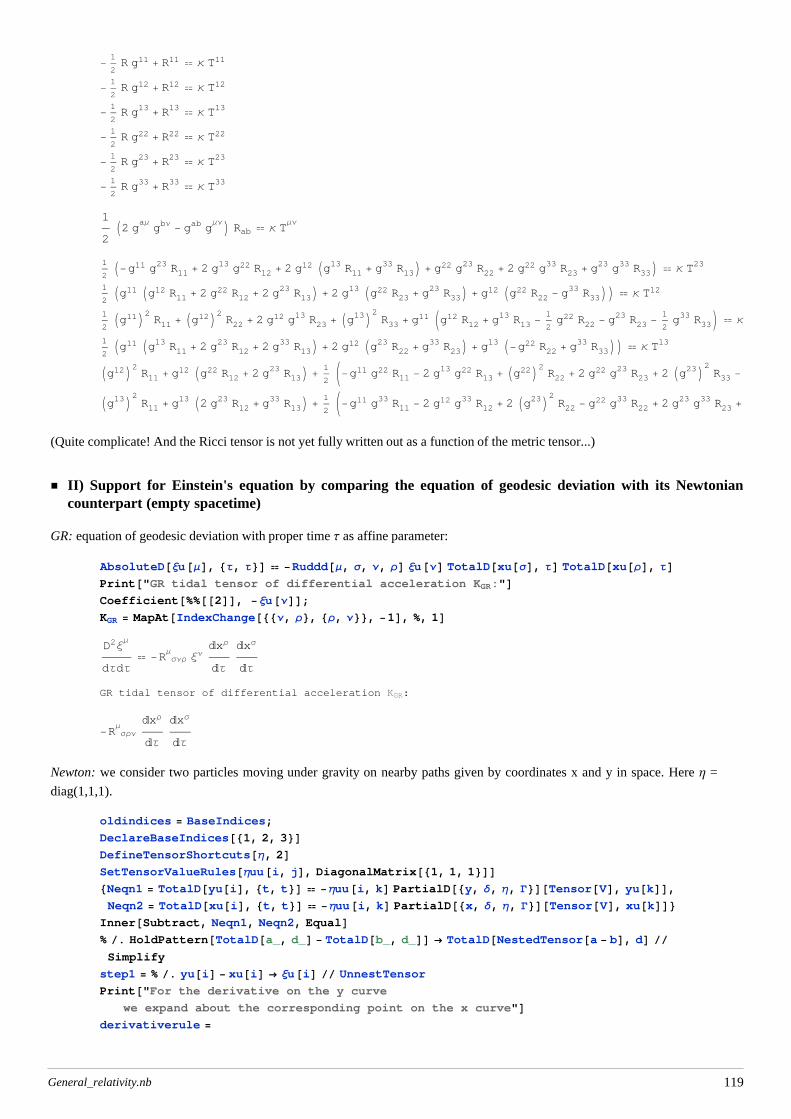
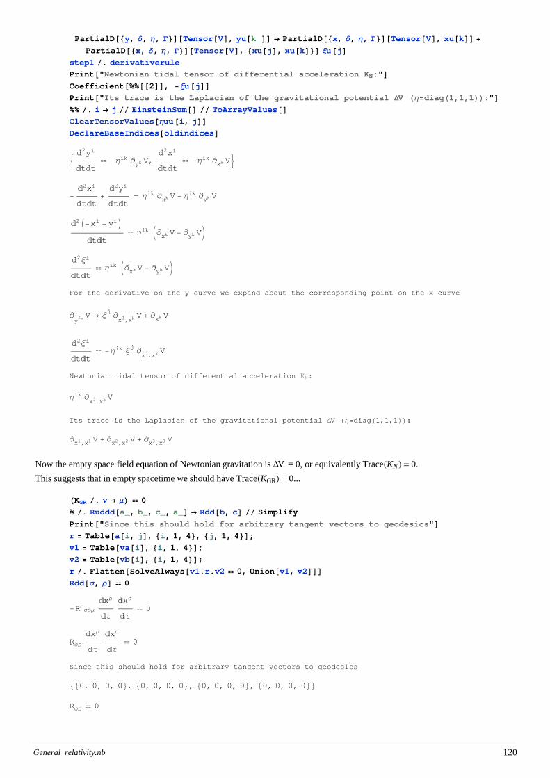
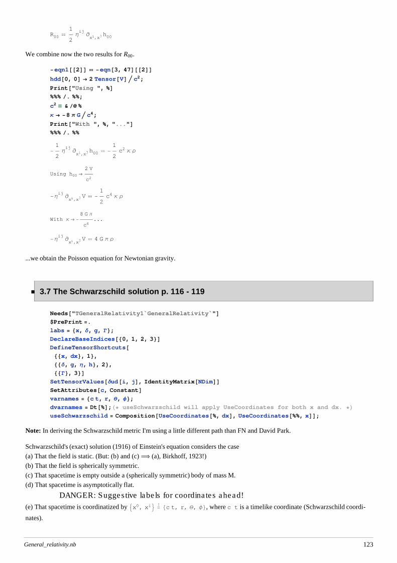
Now the empty space field equation of Newtonian gravitation is DV = 0, or equivalently TraceHKN L = 0.

This suggests that in empty spacetime we should have TraceHKGRL = 0...

HKGR . Ν ® ΜL 0

% . Ruddd@a_, b_, c_, a_D ® Rdd@b, cD Simplify

Print@"Since this should hold for arbitrary tangent vectors to geodesics"Dr = Table@a@i, jD, 8i, 1, 4<, 8j, 1, 4<D;v1 = Table@va@iD, 8i, 1, 4<D;v2 = Table@vb@iD, 8i, 1, 4<D;r . Flatten@[email protected] 0, Union@v1, v2DDDRdd@Σ, ΡD 0

-R ΣΡΜΜ

âxΡ

âΤ

âxΣ

âΤ 0

RΣΡ

âxΡ

âΤ

âxΣ

âΤ 0

Since this should hold for arbitrary tangent vectors to geodesics

880, 0, 0, 0<, 80, 0, 0, 0<, 80, 0, 0, 0<, 80, 0, 0, 0<<RΣΡ 0

This accords with Einstein's empty spacetime field equations.


This accords with Einstein's empty spacetime field equations.

III) Einstein's equation compared with Poisson's Equation (with matter)

The object here is to show that the Einstein field equations agree with the weak gravity Newtonian equations when matter is

present.

As in Section 2.7, we will use a nearly Cartesian coordinate system with gΜΝ = ΗΜΝ + hΜΝ, where hΜΝ and hΜΝ,Ρ are small, and the

extended (!?) quasi-static condition should hold: hΜΝ,0 ` hΜΝ,i and ¶x0 G 0ii small.

Print@"Stress tensor for a perfect fluid"DTuu@Μ, ΝD ITensor@ΡD + Tensor@PD c2M uu@ΜD uu@ΝD - Tensor@PD guu@Μ, ΝDPrintA"Stress tensor approximation for

a low speed Hv<<cL, low pressure HPc2<<ΡL perfect fluid."ETdd@Μ, ΝD Ρ ud@ΜD ud@ΝD;Tddapprox = LHSSymbolsToPatterns@8Μ, Ν<D@Rule %DPrint@"Raising index and contracting"Dguu@Ν, ΜD ð & %%%

% MetricSimplify@gD% . 9Tud@a_, a_D ® Tensor@TD, uu@a_D ud@a_D ® c2=;Tapprox = Rule %

Stress tensor for a perfect fluid

TΜΝ

-P gΜΝ

+P

c2+ Ρ u

ΜuΝ

Stress tensor approximation for a low speed Hv<<cL, low pressure HPc2<<ΡL perfect fluid.

TΜ_Ν_ ® Ρ uΜ uΝ

Raising index and contracting

gΝΜTΜΝ Ρ g

ΝΜuΜ uΝ

T ΝΝ Ρ uΝ u

Ν

T ® c2 Ρ

Print@"Einstein's equation eq.H3.39L in covariant form"DRdd@Μ, ΝD Κ HTdd@Μ, ΝD - 1 2 Tensor@TD gdd@Μ, ΝDLPrint@"Using the stress tensor approximation"D%% . Tddapprox . Tapprox

Print@"Taking the 00 Ricci tensor component"D%% . 8Μ ® 0, Ν ® 0<8ud@0D ® c, gdd@0, 0D ® 1<;Print@"Using ", %DHeqn@3, 47D = %%% . %%LEinstein's equation eq.H3.39L in covariant form

RΜΝ Κ -1

2T gΜΝ + TΜΝ

Using the stress tensor approximation

RΜΝ Κ -1

2c2 Ρ gΜΝ + Ρ uΜ uΝ

Taking the 00 Ricci tensor component


R00 Κ -1

2c2 Ρ g00 + Ρ Iu0M2

Using 9u0 ® c, g00 ® 1=R00

1

2c2 Κ Ρ

Print@"Riemann tensor"DEqual RiemannRule

Print@"Contracting to obtain the 00 Ricci tensor component"D%% . Thread@8a, b, c, d, e< ® 80, 0, Μ, Μ, Ν<D% . Ruddd@a_, b_, c_, a_D ® Rdd@b, cDPrintA"With small hΜΝ,Ρ, the G×G are small"E%% . Gudd@a_, _, _D Gudd@b_, _, _D ® 0

Print@"Expand into temporal and spatial parts and simplify"D%% PartialSum@0, 8i<D%%% EinsteinSum@DPrint@"Using the extended quasi-static approximation:"D%%% . PartialD@labsD@_, xu@0DD ® 0

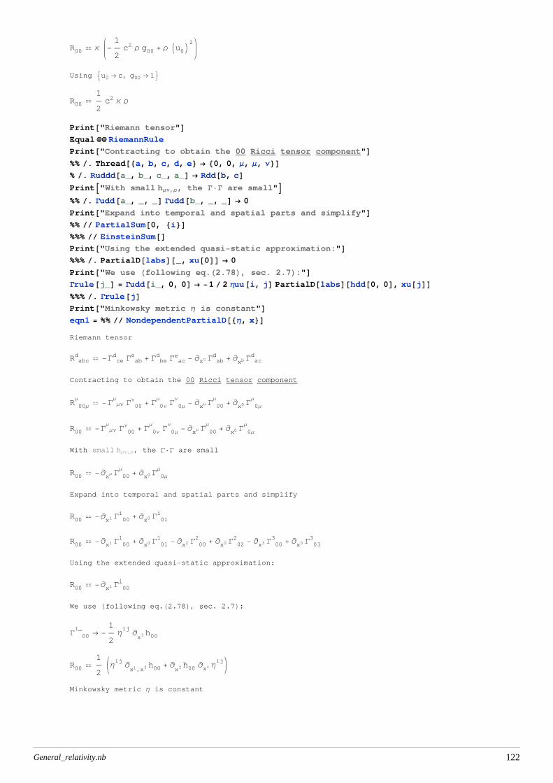
Print@"We use Hfollowing eq.H2.78L, sec. 2.7L:"DGrule@j_D = Gudd@i_, 0, 0D ® -1 2 Ηuu@i, jD PartialD@labsD@hdd@0, 0D, xu@jDD%%% . Grule@jDPrint@"Minkowsky metric Η is constant"Deqn1 = %% NondependentPartialD@8Η, x<DRiemann tensor

R abcd -G ce

d G abe + G be

d G ace - ¶xc G ab

d + ¶xb G acd

Contracting to obtain the 00 Ricci tensor component

R 00ΜΜ

-G ΜΝΜ

G 00Ν + G 0Ν

ΜG 0Μ

Ν- ¶xΜ G 00

Μ+ ¶x0 G 0Μ

Μ

R00 -G ΜΝΜ

G 00Ν + G 0Ν

ΜG 0Μ

Ν- ¶xΜ G 00

Μ+ ¶x0 G 0Μ

Μ

With small hΜΝ,Ρ, the G×G are small

R00 -¶xΜ G 00Μ

+ ¶x0 G 0ΜΜ

Expand into temporal and spatial parts and simplify

R00 -¶xi G 00i + ¶x0 G 0i

i

R00 -¶x1 G 001 + ¶x0 G 01

1 - ¶x2 G 002 + ¶x0 G 02

2 - ¶x3 G 003 + ¶x0 G 03

3

Using the extended quasi-static approximation:

R00 -¶xi G 00i

We use Hfollowing eq.H2.78L, sec. 2.7L:G 00i_

® -1

2Ηij

¶xjh00

R00 1

2KΗ

ij¶xi,xj

h00 + ¶xjh00 ¶xi Η

ijOMinkowsky metric Η is constant


R00 1

2Ηij

¶xi,xj

h00

We combine now the two results for R00.

-eqn1@@2DD -eqn@3, 47D@@2DDhdd@0, 0D ® 2 Tensor@VD c2;

Print@"Using ", %D%%% . %%;

c2 ð & %

Κ ® -8 Π G c4;

Print@"With ", %, "..."D%%% . %%

-1

2Ηij

¶xi,xj

h00 -1

2c2 Κ Ρ

Using h00 ®2 V

c2

-Ηij

¶xi,xj

V -1

2c4 Κ Ρ

With Κ ® -8 G Π

c4...

-Ηij

¶xi,xj

V 4 G Π Ρ

...we obtain the Poisson equation for Newtonian gravity.

3.7 The Schwarzschild solution p. 116 - 119


labs = 8x, ∆, g, G<;DeclareBaseIndices@80, 1, 2, 3<DDefineTensorShortcuts@88x, dx<, 1<,88∆, g, Η, h<, 2<,88G<, 3<DSetTensorValues@∆ud@i, jD, IdentityMatrix@NDimDDSetAttributes@c, ConstantDvarnames = 8c t, r, Θ, Φ<;dvarnames = Dt@%D;H* useSchwarzschild will apply UseCoordinates for both x and âx. *LuseSchwarzschild = Composition@UseCoordinates@%, dxD, UseCoordinates@%%, xDD;

Note: In deriving the Schwarzschild metric I'm using a little different path than FN and David Park.

Schwarzschild's (exact) solution (1916) of Einstein's equation considers the case

(a) That the field is static. (But: (b) and (c) (a), Birkhoff, 1923!)

(b) That the field is spherically symmetric.

(c) That spacetime is empty outside a (spherically symmetric) body of mass M.

(d) That spacetime is asymptotically flat.

DANGER: Suggestive labels for coordinates ahead!

(e) That spacetime is coordinatized by 9x0, xi= =! 8c t, r, Θ, Φ<, where c t is a timelike coordinate (Schwarzschild coordi-

nates).


Print@"Schwarzschild's ansatz for conditions HaL-HeL Hproof of uniqueness?L:"Dcmetric = DiagonalMatrixA9A@rD, -B@rD, -r2, -r2 Sin@ΘD2=E;gdd@Μ, ΝD H% MatrixFormLmetric = cmetric CoordinatesToTensors@varnamesD;SetMetricValueRules@g, metricDgdd@Μ, ΝD Hgdd@Μ, ΝD ToArrayValues@D MatrixFormLPrint@"Line element with assumed form of metric"Dds2 == gdd@Μ, ΝD dxu@ΜD dxu@ΝD% ToArrayValues@DHeqn@3, 51D = % useSchwarzschildL TraditionalForm

PrintA"A surface with constant c t and r has line element

dΣ2 and area element dS and so has the geometry of a sphere S:"EIeqn@3, 52D = IdΣ2 -eqn@3, 51D@@2DD . 8Dt@tD ® 0, Dt@rD ® 0<MM TraditionalForm

dS Ieqn@3, 52D@@2DD . Plus ® Times Sqrt PowerExpandM TraditionalForm

PrintB"àS

dS=", à-Π

Π à0

Π

%@@2DD HDt@ΘD Dt@ΦDL âΘ âΦFSchwarzschild's ansatz for conditions HaL-HeL Hproof of uniqueness?L:

gΜΝ

A@rD 0 0 00 -B@rD 0 0

0 0 -r2 0

0 0 0 -r2 Sin@ΘD2

gΜΝ

AAx1E 0 0 0

0 -BAx1E 0 0

0 0 -Ix1M20

0 0 0 -SinAx2E2 Ix1M2

Line element with assumed form of metric

ds2 dxΜdxΝ gΜΝ

ds2 AAx1E Idx0M2- BAx1E Idx1M2

- Idx2M2 Ix1M2- SinAx2E2 Idx3M2 Ix1M2

ds2 -BHrL Hâ rL2 + c2 AHrL Hâ tL2 - r2 Hâ ΘL2 - r2 Hâ ΦL2 sin2HΘLA surface with constant c t and r has line

element dΣ2 and area element dS and so has the geometry of a sphere S:

dΣ2 r2 Hâ ΘL2 + r2 Hâ ΦL2 sin2HΘLdS r2 â Θ â Φ sinHΘLàS

dS=4 Π r2

Comments:

(a): The trial solution is static because none of the metric components depend upon c t.

(b): The trial solution is spherically symmetric. The area of the sphere S is 4 Π r2, but if B[r]¹1, then r is not the radius (=

distance from center), but a "radial" coordinate.

(c): For empty spacetime we must set the Ricci tensor equal to zero.

(d): Asymptotic flatness requires that as r ® ¥, A@rD ® 1 and B@rD ® 1. Then Schwarzschild metric converges to the flat

space metric (in spherical coordinates).

Print@"Calculate the Christoffel symbols in

preparation for calculating the covariant Riemann tensor."DSetChristoffelValueRules@xu@iD, metric, GDSelectedTensorRules@G, Gudd@_, a_, b_D ; OrderedQ@8a, b<DD


SelectedTensorRules@G, Gudd@_, a_, b_D ; OrderedQ@8a, b<DD% UseCoordinates@varnamesD TableForm

Print@"Calculate the covariant Riemann

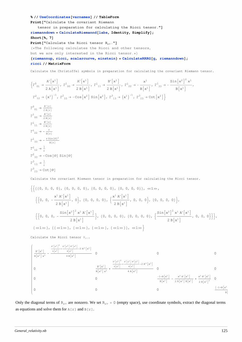
tensor in preparation for calculating the Ricci tensor."Driemanndown = CalculateRiemannd@labs, Identity, SimplifyD;Short@%, 7DPrint@"Calculate the Ricci tensor RΜΝ."DH*The following calculates the Ricci and other tensors,

but we are only interested in the Ricci tensor.*L8riemannup, ricci, scalarcurve, einstein< = CalculateRRRG@g, riemanndownD;ricci MatrixForm

Calculate the Christoffel symbols in preparation for calculating the covariant Riemann tensor.

:G 010 ®

A¢Ax1E2 AAx1E , G 00

1 ®A¢Ax1E2 BAx1E , G 11

1 ®B¢Ax1E2 BAx1E, G 22

1 ® -x1

BAx1E, G 331 ® -

SinAx2E2x1

BAx1E ,

G 122 ® Ix1M-1

, G 332 ® -CosAx2E SinAx2E, G 13

3 ® Ix1M-1, G 23

3 ® CotAx2E>G 010 ®

A¢@rD2 A@rD

G 001 ®

A¢@rD2 B@rD

G 111 ®

B¢@rD2 B@rD

G 221 ® -

r

B@rDG 331 ® -

r Sin@ΘD2B@rD

G 122 ®

1

r

G 332 ® -Cos@ΘD Sin@ΘD

G 133 ®

1

r

G 233 ® Cot@ΘD

Calculate the covariant Riemann tensor in preparation for calculating the Ricci tensor.

::880, 0, 0, 0<, 80, 0, 0, 0<, 80, 0, 0, 0<, 80, 0, 0, 0<<, 1,

::0, 0, -x1 A¢Ax1E2 BAx1E , 0>, 80, 0, 0, 0<, : x1 A¢Ax1E

2 BAx1E , 0, 0, 0>, 80, 0, 0, 0<>,

::0, 0, 0, -SinAx2E2

x1 A¢Ax1E2 BAx1E >, 80, 0, 0, 0<, 80, 0, 0, 0<, :SinAx2E2

x1 A¢Ax1E2 BAx1E , 0, 0, 0>>>,

81<, 881<, 81<, 81<, 81<<, 1>Calculate the Ricci tensor RΜΝ.

A¢Ax1EBAx1E x1

-

A¢Bx1F2ABx1F +

A¢Bx1F B¢Bx1FBBx1F -2 A¢¢Ax1E4 BAx1E 0 0 0

0B¢Ax1EBAx1E x1

+

A¢Bx1F2ABx1F +

A¢Bx1F B¢Bx1FBBx1F -2 A¢¢Ax1E4 AAx1E 0 0

0 0-1+BAx1EBAx1E -

x1 A¢Ax1E2 AAx1E BAx1E +

x1 B¢Ax1E2 BAx1E2 0

0 0 0I-1+BAx1E

BAOnly the diagonal terms of RΜΝ are nonzero. We set RΜΝ = 0 (empty space), use coordinate symbols, extract the diagonal terms

as equations and solve them for A[r] and B[r].


8eqn@3, 54D, eqn@3, 55D, eqn@3, 56D, eqn@3, 57D<;HTr@Simplify@ricci UseCoordinates@varnamesDD, ListD 80, 0, 0, 0< Thread SimplifyL;8%%, %<;

Transpose@%D TableForm

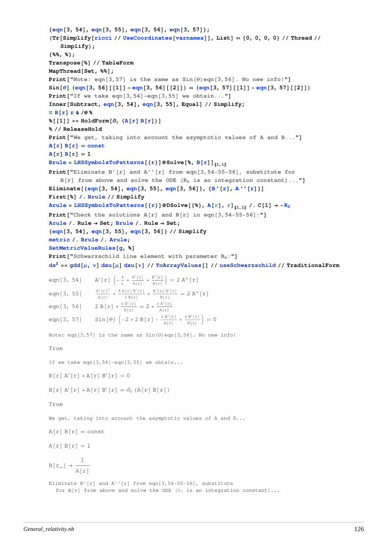
MapThread@Set, %%D;Print@"Note: eqn@3,57D is the same as SinHΘLeqn@3,56D. No new info!"DSin@ΘD Heqn@3, 56D@@1DD - eqn@3, 56D@@2DDL Heqn@3, 57D@@1DD - eqn@3, 57D@@2DDLPrint@"If we take eqn@3,54D-eqn@3,55D we obtain..."DInner@Subtract, eqn@3, 54D, eqn@3, 55D, EqualD Simplify;

ð B@rD r & %

%@@1DD == HoldForm@¶r HA@rD B@rDLD% ReleaseHold

Print@"We get, taking into account the asymptotic values of A and B..."DA@rD B@rD const

A@rD B@rD 1

Brule = LHSSymbolsToPatterns@8r<DSolve@%, B@rDDP1,1TPrint@"Eliminate B'@rD and A''@rD from eqn@3,54-55-56D, substitute for

B@rD from above and solve the ODE HRS is an integration constantL..."DEliminate@8eqn@3, 54D, eqn@3, 55D, eqn@3, 56D<, 8B'@rD, A''@rD<DFirst@%D . Brule Simplify

Arule = LHSSymbolsToPatterns@8r<DDSolve@8%<, A@rD, rDP1,1T . C@1D ® -RS

Print@"Check the solutions A@rD and B@rD in eqn@3,54-55-56D:"DArule . Rule ® Set; Brule . Rule ® Set;8eqn@3, 54D, eqn@3, 55D, eqn@3, 56D< Simplify

metric . Brule . Arule;

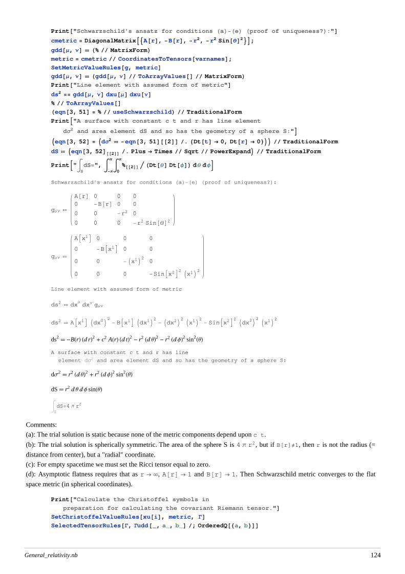
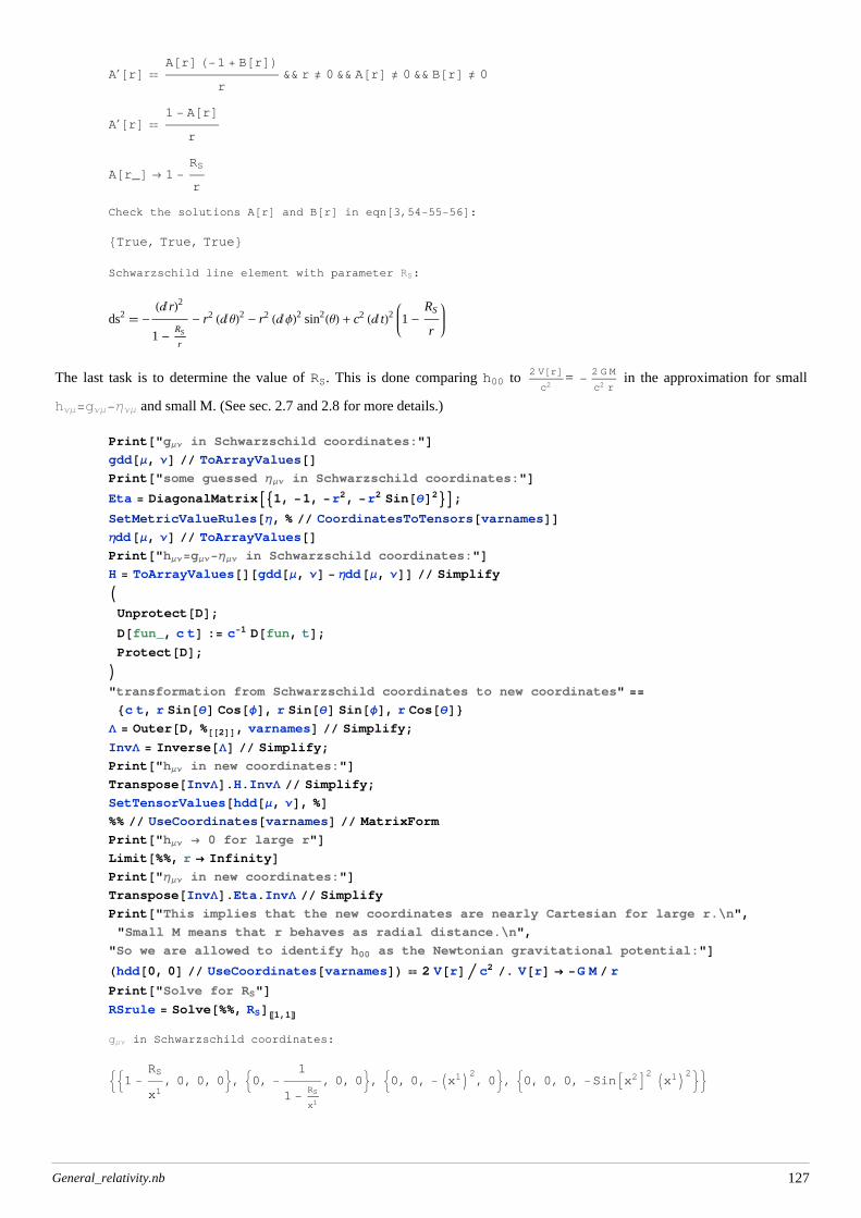
SetMetricValueRules@g, %DPrint@"Schwarzschild line element with parameter RS:"Dds2 == gdd@Μ, ΝD dxu@ΜD dxu@ΝD ToArrayValues@D useSchwarzschild TraditionalForm

eqn@3, 54D A¢@rD J-4

r+

A¢@rDA@rD +

B¢@rDB@rD N 2 A¢¢@rD

eqn@3, 55D A¢@rD2A@rD +

4 A@rD B¢@rDr B@rD +

A¢@rD B¢@rDB@rD 2 A¢¢@rD

eqn@3, 56D 2 B@rD +r B¢@rDB@rD 2 +

r A¢@rDA@rD

eqn@3, 57D Sin@ΘD J-2 + 2 B@rD -r A¢@rDA@rD +

r B¢@rDB@rD N 0

Note: eqn@3,57D is the same as SinHΘLeqn@3,56D. No new info!

True

If we take eqn@3,54D-eqn@3,55D we obtain...

B@rD A¢@rD + A@rD B¢@rD 0

B@rD A¢@rD + A@rD B¢@rD ¶rHA@rD B@rDLTrue

We get, taking into account the asymptotic values of A and B...

A@rD B@rD const

A@rD B@rD 1

B@r_D ®1

A@rDEliminate B'@rD and A''@rD from eqn@3,54-55-56D, substitute

for B@rD from above and solve the ODE HRS is an integration constantL...


A¢@rD A@rD H-1 + B@rDL

r&& r ¹ 0 && A@rD ¹ 0 && B@rD ¹ 0

A¢@rD 1 - A@rD

r

A@r_D ® 1 -RS

r

Check the solutions A@rD and B@rD in eqn@3,54-55-56D:8True, True, True<Schwarzschild line element with parameter RS:

ds2 -Hâ rL2

1 -RS

r

- r2 Hâ ΘL2 - r2 Hâ ΦL2 sin2HΘL + c2 Hâ tL2 1 -RS

r

The last task is to determine the value of RS. This is done comparing h00 to 2 V@rDc2

= - 2 G M

c2 r in the approximation for small

hΝΜ=gΝΜ-ΗΝΜ and small M. (See sec. 2.7 and 2.8 for more details.)

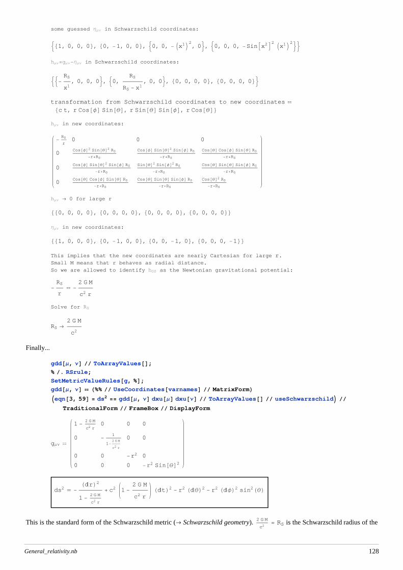
Print@"gΜΝ in Schwarzschild coordinates:"Dgdd@Μ, ΝD ToArrayValues@DPrint@"some guessed ΗΜΝ in Schwarzschild coordinates:"DEta = DiagonalMatrixA91, -1, -r2, -r2 Sin@ΘD2=E;SetMetricValueRules@Η, % CoordinatesToTensors@varnamesDDΗdd@Μ, ΝD ToArrayValues@DPrint@"hΜΝ=gΜΝ-ΗΜΝ in Schwarzschild coordinates:"DH = ToArrayValues@D@gdd@Μ, ΝD - Ηdd@Μ, ΝDD SimplifyIUnprotect@DD;D@fun_, c tD := c-1 D@fun, tD;Protect@DD;M

"transformation from Schwarzschild coordinates to new coordinates" ==8c t, r Sin@ΘD Cos@ΦD, r Sin@ΘD Sin@ΦD, r Cos@ΘD<L = Outer@D, %@@2DD, varnamesD Simplify;

InvL = Inverse@LD Simplify;

Print@"hΜΝ in new coordinates:"[email protected] Simplify;

SetTensorValues@hdd@Μ, ΝD, %D%% UseCoordinates@varnamesD MatrixForm

Print@"hΜΝ ® 0 for large r"DLimit@%%, r ® InfinityDPrint@"ΗΜΝ in new coordinates:"[email protected] Simplify

Print@"This implies that the new coordinates are nearly Cartesian for large r.\n",

"Small M means that r behaves as radial distance.\n",

"So we are allowed to identify h00 as the Newtonian gravitational potential:"DHhdd@0, 0D UseCoordinates@varnamesDL 2 V@rD c2 . V@rD ® -G M r

Print@"Solve for RS"DRSrule = Solve@%%, RSDP1,1TgΜΝ in Schwarzschild coordinates:

::1 -RS

x1, 0, 0, 0>, :0, -

1

1 -RS

x1

, 0, 0>, :0, 0, -Ix1M2, 0>, :0, 0, 0, -SinAx2E2 Ix1M2>>


some guessed ΗΜΝ in Schwarzschild coordinates:

:81, 0, 0, 0<, 80, -1, 0, 0<, :0, 0, -Ix1M2, 0>, :0, 0, 0, -SinAx2E2 Ix1M2>>

hΜΝ=gΜΝ-ΗΜΝ in Schwarzschild coordinates:

::-RS

x1, 0, 0, 0>, :0, RS

RS - x1, 0, 0>, 80, 0, 0, 0<, 80, 0, 0, 0<>

transformation from Schwarzschild coordinates to new coordinates 8c t, r Cos@ΦD Sin@ΘD, r Sin@ΘD Sin@ΦD, r Cos@ΘD<hΜΝ in new coordinates:

-RS

r0 0 0

0Cos@ΦD2 Sin@ΘD2 RS

-r+RS

Cos@ΦD Sin@ΘD2 Sin@ΦD RS

-r+RS

Cos@ΘD Cos@ΦD Sin@ΘD RS

-r+RS

0Cos@ΦD Sin@ΘD2 Sin@ΦD RS

-r+RS

Sin@ΘD2 Sin@ΦD2 RS-r+RS

Cos@ΘD Sin@ΘD Sin@ΦD RS

-r+RS

0Cos@ΘD Cos@ΦD Sin@ΘD RS

-r+RS

Cos@ΘD Sin@ΘD Sin@ΦD RS

-r+RS

Cos@ΘD2 RS-r+RS

hΜΝ ® 0 for large r

880, 0, 0, 0<, 80, 0, 0, 0<, 80, 0, 0, 0<, 80, 0, 0, 0<<ΗΜΝ in new coordinates:

881, 0, 0, 0<, 80, -1, 0, 0<, 80, 0, -1, 0<, 80, 0, 0, -1<<This implies that the new coordinates are nearly Cartesian for large r.Small M means that r behaves as radial distance.

So we are allowed to identify h00 as the Newtonian gravitational potential:

-RS

r -

2 G M

c2 r

Solve for RS

RS ®2 G M

c2

Finally...

gdd@Μ, ΝD ToArrayValues@D;% . RSrule;

SetMetricValueRules@g, %D;gdd@Μ, ΝD H%% UseCoordinates@varnamesD MatrixFormLIeqn@3, 59D = ds2 == gdd@Μ, ΝD dxu@ΜD dxu@ΝD ToArrayValues@D useSchwarzschildM

TraditionalForm FrameBox DisplayForm

gΜΝ

1 -2 G M

c2 r0 0 0

0 -1

1-2 G M

c2 r

0 0

0 0 -r2 0

0 0 0 -r2 Sin@ΘD2

ds2 -HârL2

1 -2 G M

c2 r

+ c2 1 -2 G M

c2 rHâtL2 - r2 HâΘL2 - r2 HâΦL2 sin2HΘL

This is the standard form of the Schwarzschild metric (® Schwarzschild geometry). 2 G Mc2

= RS is the Schwarzschild radius of the

mass M.


This is the standard form of the Schwarzschild metric (® Schwarzschild geometry). 2 G Mc2

= RS is the Schwarzschild radius of the

mass M.

H* The Schwarzschild radius of some objects. *LRS@M_H*kg*LDH*m*L = RSrule@@2DD . 9G ® 6.674 ´ 10-11, c ® 299792 458=;data = :

:"12

solar mass neutron star", mSun 2, 104>,9"white dwarf H~Sirius BL", mSun, 5.750 106=,9"Sun", mSun = 1.989 1030H*kg*L, 6.960 108H*m*L=,9"Earth", 5.976 1024, 6.3710 106=, :"me Hoctober 2011L", mme = 77, 3 mme 10

-3 H4 ΠL3 >,:"proton", 1.67 ´ 10-27, 0.74 10-15>>;

RS@ð D & Hð@@2DD & dataL;RS@ð D & Hð@@2DD & dataL;% Hð@@3DD & dataL;Prepend @Transpose@8Hð@@1DD & dataL, %%, %<D,8"Object", "RS HmL", "RSrsurface"<D TableForm

Object RS HmL RSrsurface1

2solar mass neutron star 1477. 0.1477

white dwarf H~Sirius BL 2953.99 0.000513738

Sun 2953.99 4.24424 ´ 10-6

Earth 0.00887535 1.39309 ´ 10-9

me Hoctober 2011L 1.14358 ´ 10-25 4.33309 ´ 10-25

proton 2.48023 ´ 10-54 2.8832 ´ 10-39

Chapter 4: Physics in the vicinity of a massive object


FN: "Turning M up introduces curvature, so that spacetime is no longer flat, and there is no reason to assume that the coordinates

have the simple physical meanings they had in flat spacetime."

Ranges of the Schwarzschild coordinates :

t Î H-¥, +¥LΘ Î @0, ΠD, Φ Î @0, 2 ΠL with Φ + integer 2 Π º Φ

maxHrB, RSL, +¥L where rB is the boundary of the object

In the next subsections we investigate the relationship between coordinates and physically observable quantities in the framework

of the static spacetime given by the Schwarzschild solution.

4.1 Length and time p. 124

"Chuck Norris doesn’t wear a watch, HE decides what time it is."


labs = 8x, ∆, g, G<;DeclareBaseIndices@80, 1, 2, 3<D


DeclareBaseIndices@80, 1, 2, 3<DDefineTensorShortcuts@88x, dx<, 1<,88∆, g<, 2<,88G<, 3<DSetAttributes@c, ConstantDvarnames = 8c t, r, Θ, Φ<;dvarnames = Dt@%D;useSchwarzschild = Composition MapThread@UseCoordinates@ð1, ð2D &, 88%, %%<, 8dx, x<<D;box = Composition@DisplayForm, FrameBox, TraditionalFormD;H* Def. of Schwarzschild metric *LDiagonalMatrixB:1 - 2 G M Ic2 rM, -I1 - 2 G M Ic2 rMM-1

, -r2, -r2 Sin@ΘD2>F . IM ® m c2 GM;SetMetricValueRules@g, % CoordinatesToTensors@varnamesDD;

1) We rewrite the spacetime line element in the Schwarzschild metric as function of observable quantities.

Print@"Spacetime line element in Schwarzschild metric eq.H4.1L,p.124"Dds2 == c2 dΤ2 gdd@Μ, ΝD dxu@ΜD dxu@ΝDHeqn@4, 1D = %@@81, 3<DD ToArrayValues@D useSchwarzschildL box

PrintA"- Space line element at fixed time Hsign change!L eq.H4.2),p.124"Edl2 H-gdd@Μ, ΝD dxu@ΜD dxu@ΝD ToArrayValues@81, 2, 3<D useSchwarzschildL

HoldFormAdR2 + dL2EPrint@"-- tangential line element eq.H4.4L,p.125"DdL2 -gdd@Μ, ΝD dxu@ΜD dxu@ΝD ToArrayValues@82, 3<D Simplify useSchwarzschildHeqn@4, 4D = Sqrt % PowerExpandL box

Print@"-- radial line element eq.H4.5L,p.125"DdR2 -gdd@Μ, ΝD dxu@ΜD dxu@ΝD ToArrayValues@81<D useSchwarzschild

%@@1DD == HoldFormAEvaluateASeriesA%@@2DD Dt@rD2, 8r, ¥, 3<EEE HoldFormADt@rD2E TraditionalFormHeqn@4, 5D = Sqrt %% PowerExpandL box

Print@"- Proper time line element at fixed point in space eq.H4.6L,p.127"Dc2 dT2 gdd@Μ, ΝD dxu@ΜD dxu@ΝD ToArrayValues@80<D useSchwarzschild

%@@1DD == HoldFormAEvaluateASeriesA%@@2DD Dt@tD2, 8r, ¥, 3<EEE HoldFormADt@tD2E TraditionalFormIeqn@4, 6D = SqrtAð c2E & %% PowerExpandM box

Print@"Hence the spacetime line element in the Schwarzschild metric is:"Dds2 HoldFormAc2 dT2 - IdR2 + dL2ME% . H8eqn@4, 1D, eqn@4, 4D, eqn@4, 5D, eqn@4, 6D< . Equal ® RuleL ReleaseHold Simplify

Spacetime line element in Schwarzschild metric eq.H4.1L,p.124ds2 c2 dΤ2 dx

ΜdxΝ gΜΝ

ds2 -HârL2

1 -2 m

r

+ c2 1 -2 m

rHâtL2 - r2 HâΘL2 - r2 HâΦL2 sin2HΘL

- Space line element at fixed time Hsign change!L eq.H4.2),p.124dl2

Dt@rD2

1 -2 m

r

+ r2 Dt@ΘD2 + r2 Dt@ΦD2 Sin@ΘD2 dR2 + dL2

-- tangential line element eq.H4.4L,p.125dL2 r2 IDt@ΘD2 + Dt@ΦD2 Sin@ΘD2M


dL r HâΘL2 + HâΦL2 sin2HΘL-- radial line element eq.H4.5L,p.125dR2

Dt@rD2

1 -2 m

r

dR2 Hâ rL2 1 +2 m

r+ 4 m2

1

r

2

+ 8 m31

r

3

+ O1

r

4

dR âr

1 -2 m

r

- Proper time line element at fixed point in space eq.H4.6L,p.127c2 dT2 c2 1 -

2 m

rDt@tD2

c2 dT2 Hâ tL2 c2 -2 Ic2 mM

r+ O

1

r

4

dT 1 -2 m

rât

Hence the spacetime line element in the Schwarzschild metric is:

ds2 c2 dT2 - IdR2 + dL2MTrue

Coordinate distance of concentric spheres: surface S(r) < S(r+Dr), DS = S(r+Dr)-S(r). Dr¹DR !

ReduceA9DS 4 Π Hr + DrL2 - 4 Π r2 && Dr > 0 && r > 0 && DS > 0=, DrE@@3DD

Dr -r +4 Π r2 + DS

2 Π

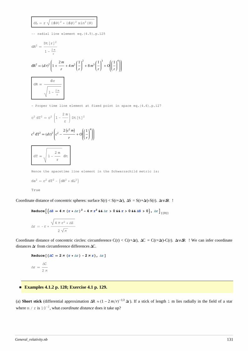
Coordinate distance of concentric circles: circumference C(r) < C(r+Dr), DC = C(r+Dr)-C(r). Dr¹DR ! We can infer coordinate

distances Dr from circumference differences DC.

Reduce@8DC 2 Π Hr + DrL - 2 Π r<, DrDDr

DC

2 Π

Examples 4.1.2 p. 128; Exercise 4.1 p. 129.

(a) Short stick (differential approximation DR » H1 - 2 m rL-12 Dr ). If a stick of length 1 m lies radially in the field of a star

where m r is 10-2, what coordinate distance does it take up?


eqn@4, 5DSolveA% . 9m r ® 10-2, dR ® 1=E N

res = %@@1, 1, 2DD;dR

Dt@rD1 -

2 m

r

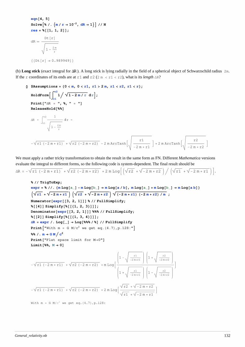
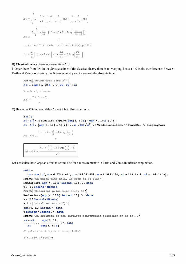
88Dt@rD ® 0.989949<<(b) Long stick (exact integral for DR ). A long stick is lying radially in the field of a spherical object of Schwarzschild radius 2m.

If the r coordinates of its ends are at r1 and r2 (2 m < r1 < r2), what is its length DR?

Ý $Assumptions = 80 < m, 0 < r1, r1 > 2 m, r1 < r2, r1 < r<;HoldFormBà

r1

r2

1 1 - 2 m r ârF;Print@"DR = ", %, " = "DReleaseHold@%%DDR = à

r1

r2 1

1 -2 m

r

âr =

- r1 H-2 m + r1L + r2 H-2 m + r2L - 2 m ArcTanhB r1

-2 m + r1F + 2 m ArcTanhB r2

-2 m + r2F

We must apply a rather tricky transformation to obtain the result in the same form as FN. Different Mathematica versions

evaluate the integral to different forms, so the following code is system-dependent. The final result should be

DR = - r1 H-2 m + r1L + r2 H-2 m + r2L + 2 m LogBJ r2 + -2 m + r2 N J r1 + -2 m + r1 NF.

% TrigToExp;

expr = % . 8m Log@a_D - m Log@b_D ® m Log@a bD, m Log@a_D + m Log@b_D ® m Log@a bD<J r1 + -2 m + r1 N J r2 + -2 m + r2 N H-2 m + r1L H-2 m + r2L m ;

Numerator@expr@@3, 2, 1DDD % FullSimplify;

%@@4DD Simplify@%@@81, 2, 3<DDD;Denominator@expr@@3, 2, 1DDD %%% FullSimplify;

%@@2DD Simplify@%@@81, 3, 4<DDD;DR = expr . Log@_D ® Log@%%% %D FullSimplify

PrintA"With m = G Mc2 we get eq.H4.7L,p.128:"E%% . m ® G M c2

Print@"Flat space limit for M®0"DLimit@%%, M ® 0D

- r1 H-2 m + r1L + r2 H-2 m + r2L + m LogB1 -

r1

-2 m+r11 +

r2

-2 m+r2

1 +r1

-2 m+r11 -

r2

-2 m+r2

F

- r1 H-2 m + r1L + r2 H-2 m + r2L + 2 m LogB r2 + -2 m + r2

r1 + -2 m + r1F

With m = G Mc2 we get eq.H4.7L,p.128:


- r1 -2 G M

c2+ r1 + r2 -

2 G M

c2+ r2 +

2 G M LogB r2 + -2 G M

c2+r2

r1 + -2 G M

c2+r1

Fc2

Flat space limit for M®0

-r1 + r2

Check differential approximation in example 4.1.2(a) with the exact formula for DR calculated in example 4.1.2(b):

DR . 9m ® 10-2, r1 ® 1 - res 2, r2 ® 1 + res 2=1 + 8-res, +res< 2

FindRootAIDR . 9m ® 10-2, r1 ® %@@1DD=M 1, 8r2, 1<E1.001

80.505025, 1.49497<8r2 ® 1.49398<

Extra space ES between the orbits of Earth and Venus in the gravitational field of the Sun. (Extra Raum ES zwischen den

Bahnen von Erde und Venus im Sonnenschwerefeld.):

data = 9m ® G M c2, G ® 6.674*^-11, c ® 299792 458,

M ® H*MSun=*L1.989*^30, r1 ® H*rVenus=*L108.2*^9, r2 ® H*rEarth=*L149.6*^9=;ES = HDR - Hr2 - r1LL Meter . data

ES HDR MeterL . data

ES Hc Meter SecondL . data

478.523 Meter

1.15585 ´ 10-8

1.59618 ´ 10-6 Second

4.2 Radar sounding (Shapiro-Effekt) p. 129


labs = 8x, ∆, g, G<;DeclareBaseIndices@80, 1, 2, 3<DDefineTensorShortcuts@88x, dx<, 1<,88∆, g<, 2<,88G<, 3<DSetAttributes@c, ConstantDvarnames = 8c t, r, Θ, Φ<;dvarnames = Dt@%D;useSchwarzschild = Composition@UseCoordinates@%, dxD, UseCoordinates@%%, xDD;H* Def. of Schwarzschild metric *LDiagonalMatrixB:1 - 2 G M Ic2 rM, -I1 - 2 G M Ic2 rMM-1

, -r2, -r2 Sin@ΘD2>F . IM ® m c2 GM;SetMetricValueRules@g, % CoordinatesToTensors@varnamesDD;

When Venus and Earth are line up with the sun a radar pulse is bounced off Venus from Earth. The proper time lapse DΤ for the

whole trip as measured by the observer on Earth is compared with the expected value DΤ from classical theory. (Irwin I. Shapiro,

December 1964, "Fourth Test of General Relativity", Physical Review Letters 13: 789–791; first detection in 1968.)


When Venus and Earth are line up with the sun a radar pulse is bounced off Venus from Earth. The proper time lapse DΤ for the

whole trip as measured by the observer on Earth is compared with the expected value DΤ from classical theory. (Irwin I. Shapiro,

December 1964, "Fourth Test of General Relativity", Physical Review Letters 13: 789–791; first detection in 1968.)

A) General relativity: two-way travel time DΤ

Print@"Spacetime line element in Schwarzschild metric"DDt@sD2 == c2 Dt@ΤD2 gdd@Μ, ΝD dxu@ΜD dxu@ΝDH% ToArrayValues@D useSchwarzschildL Rest

Print@"For fixed Θ and Φ Hinferior conjunctionL and using dΤ 0 for a radar pulse we get"DH%% . 8Dt@ΤD ® 0, Dt@ΘD ® 0, Dt@ΦD ® 0<L

Print@"Solve for the coordinate speed of light in the radial direction c@rDHNote: 2m < rL"D

Map@ð Dt@tD &, Solve@%%, Dt@rDD Flatten, 82<DIc@rD = %@@1,2DDM -%@@2,2DD Simplify

Print@"The two-way travel time from Earth Hr1L to

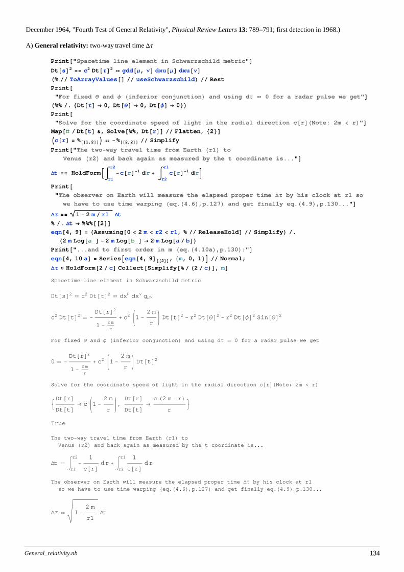
Venus Hr2L and back again as measured by the t coordinate is..."DDt == HoldFormBà

r1

r2

-c@rD-1 âr + àr2

r1

c@rD-1 ârFPrint@"The observer on Earth will measure the elapsed proper time DΤ by his clock at r1 so

we have to use time warping Heq.H4.6L,p.127L and get finally eq.H4.9L,p.130..."DDΤ == 1 - 2 m r1 Dt

% . Dt ® %%%@@2DDeqn@4, 9D = HAssuming@0 < 2 m < r2 < r1, % ReleaseHoldD SimplifyL .H2 m Log@a_D - 2 m Log@b_D ® 2 m Log@a bDLPrint@"...and to first order in m Heq.H4.10aL,p.130L:"Deqn@4, 10 aD = SeriesAeqn@4, 9D@@2DD, 8m, 0, 1<E Normal;

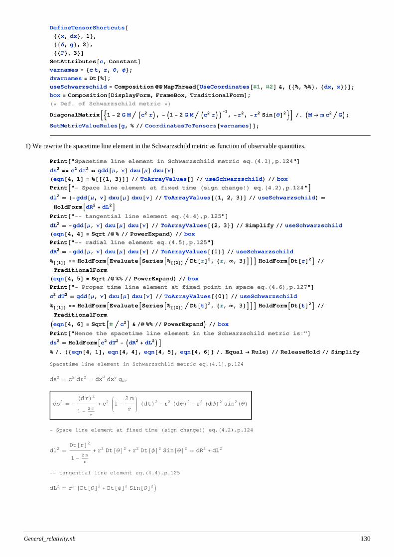
DΤ » HoldForm@2 cD Collect@Simplify@% H2 cLD, mDSpacetime line element in Schwarzschild metric

Dt@sD2 c2 Dt@ΤD2 dxΜdxΝ gΜΝ

c2 Dt@ΤD2 -Dt@rD2

1 -2 m

r

+ c2 1 -2 m

rDt@tD2 - r2 Dt@ΘD2 - r2 Dt@ΦD2 Sin@ΘD2

For fixed Θ and Φ Hinferior conjunctionL and using dΤ 0 for a radar pulse we get

0 -Dt@rD2

1 -2 m

r

+ c2 1 -2 m

rDt@tD2

Solve for the coordinate speed of light in the radial direction c@rDHNote: 2m < rL:Dt@rDDt@tD ® c 1 -

2 m

r,Dt@rDDt@tD ®

c H2 m - rLr

>True

The two-way travel time from Earth Hr1L to

Venus Hr2L and back again as measured by the t coordinate is...

Dt àr1

r2

-1

c@rD âr + àr2

r1 1

c@rD âr

The observer on Earth will measure the elapsed proper time DΤ by his clock at r1

so we have to use time warping Heq.H4.6L,p.127L and get finally eq.H4.9L,p.130...

DΤ 1 -2 m

r1Dt


DΤ 1 -2 m

r1àr1

r2

-1

c@rD âr + àr2

r1 1

c@rD âr

DΤ

2 1 -2 m

r1Jr1 - r2 + 2 m LogB -2 m+r1

-2 m+r2FN

c

...and to first order in m Heq.H4.10aL,p.130L:DΤ »

2

cr1 - r2 + m -1 +

r2

r1+ 2 LogB r1

r2F

B) Classical theory: two-way travel time D Τ

I depart here from FN. In the flat spacetime of the classical theory there is no warping, hence r1-r2 is the true distances between

Earth and Venus as given by Euclidean geometry and t measures the absolute time.

PrintA"Round-trip time DΤ"ED Τ Heqn@4, 10 bD = 2 Hr1 - r2L cLRound-trip time DΤ

D Τ 2 Hr1 - r2L

c

C) Hence the GR-induced delay DΤ - D Τ is to first order in m:

2 m c;

DΤ - D Τ » % Simplify@Expand@eqn@4, 10 aD - eqn@4, 10 bDD %DDΤ - D Τ » Ieqn@4, 11D = %@@2DD . m ® G M c2M TraditionalForm FrameBox DisplayForm

DΤ - D Τ »2 m J-1 +

r2

r1+ 2 LogB r1

r2FN

c

DΤ - D Τ »2 G M J r2

r1+ 2 logJ r1

r2N - 1N

c3

Let's calculate how large an effect this would be for a measurement with Earth and Venus in inferior conjunction.

data =9m ® G M c2, G ® 6.674*^-11, c ® 299 792 458, M ® 1.989*^30, r1 ® 149.6*^9, r2 ® 108.2*^9=;Print@"GR pulse time delay DΤ from eq.H4.10aL"DNumberForm@eqn@4, 10 aD Second, 10D . data

% H60 Second MinuteLPrintA"Classical pulse time delay DΤ"ENumberForm@eqn@4, 10 bD Second, 10D . data

% H60 Second MinuteLPrintA"DΤ-DΤ and cHDΤ-DΤL"Eeqn@4, 11D Second . data

% c Meter Second . data

Print@"An estimate of the required measurement precision on DΤ is..."DDΤ - D Τ

DΤ==

eqn@4, 11Deqn@4, 10 aD . data

GR pulse time delay DΤ from eq.H4.10aL276.1910745 Second


4.60318 Minute

Classical pulse time delay DΤ

276.1910708 Second

4.60318 Minute

DΤ-DΤand cHDΤ-DΤ

L3.6579 ´ 10-6 Second

1096.61 Meter

An estimate of the required measurement precision on DΤ is...

DΤ - D Τ

DΤ 1.32441 ´ 10-8

4.3 Spectral Shift p. 131


labs = 8x, ∆, g, G<;DeclareBaseIndices@80, 1, 2, 3<DDefineTensorShortcuts@88x, dx<, 1<,88∆, g<, 2<,88G<, 3<DSetAttributes@c, ConstantD

æ 1) General case: Suppose that in a static spacetime a signal is sent from an emitter E at a fixed point, that it travels along a

null geodesic and is received by a receiver R at a fixed point.

Print@"Line element in spacetime:"Dds2 gdd@Μ, ΝD dxu@ΜD dxu@ΝDPrint@"Line element along a null geodesic:"D%% . ds ® 0

PrintA"Null geodesic with affine parametrization xΜHuL, u Î @uE,uRD. Divide by du2."E%% . dxu@i_D ¦ TotalD@xu@iD, uDPrint@"Expand into temporal and spatial parts."DMapAt@PartialSum@0, 8i, j<D, %%, 2DPrint@"In a suitably defined coordinate system the mixed metric components

gi0 of a static spacetime are zero HLandau,vol.II,chap.10,par.88L."D%% . 8gdd@i, 0D ® 0, gdd@0, jD ® 0<PrintB"Solve for the coordinate time component.HÜ: a2 L"FReverse@%%D;ð - Part@%, 1, 2D & %

ð gdd@0, 0D & %

ð & %

MapAt@PowerExpand, %, 1DPrintA"Substitute variable x0HuL=c tHuL and simplify."E%% . Tensor@x, List@0D, List@VoidDD ® c t@uDð c & %

Print@"Integrate. We get the coordinate time of travel:"DIntegrate@ð, 8u, u"E", uR<D & %%


Line element in spacetime:

ds2 dxΜdxΝ gΜΝ

Line element along a null geodesic:

0 dxΜdxΝ gΜΝ

Null geodesic with affine parametrization xΜHuL, u Î @uE,uRD. Divide by du2.

0 gΜΝ

âxΜ

âu

âxΝ

âu

Expand into temporal and spatial parts.

0 g00

âx0

âu

2

+ gi0

âx0

âu

âxi

âu+ g0j

âx0

âu

âxj

âu+ gij

âxi

âu

âxj

âu

In a suitably defined coordinate system the mixed metric

components gi0 of a static spacetime are zero HLandau,vol.II,chap.10,par.88L.0 g00

âx0

âu

2

+ gijâxi

âu

âxj

âu

Solve for the coordinate time component.HÜ: a2 Lg00

âx0

âu

2

-gijâxi

âu

âxj

âu

âx0

âu

2

-gij

âxi

âu

âxj

âu

g00

âx0

âu

2

-gij

âxi

âu

âxj

âu

g00

âx0

âu -

gijâxi

âu

âxj

âu

g00

Substitute variable x0HuL=c tHuL and simplify.

c t¢@uD -gij

âxi

âu

âxj

âu

g00

t¢@uD

-gij

âxi

âu

âxj

âu

g00

c

Integrate. We get the coordinate time of travel:


-t@uED + t@uRD àuE

uR

-gij

âxi

âu

âxj

âu

g00

câu

The coordinate time delay tR - tE between emission and reception depends only on the chosen spatial path between the two

spatial points. (We don't actually care about the time of travel so we don't have to evaluate the integral.) For two signals 1 and 2

travelling on the same path we have tR1 - tE1 = tR2 - tE2, hence we get always DtR º tR2 - tR1 = tE2 - tE1 º DtE.

PrintB"Proper time delays between two signals in R and E:\n8DΤR,DΤE<=",

:DΤR = c-1 gdd@0, 0DR DtR,

DΤ"E" = c-1 gdd@0, 0D"E" Dt"E">FPrint@"Gravitational spectral shift in a static spacetime:"DΝR Ν"E" Hdummy = HoldForm@ n DΤRD HoldForm@ n DΤ"E"DL ==Hdummy ReleaseHoldL . DtR ® Dt"E" FrameBox DisplayForm

Proper time delays between two signals in R and E:

8DΤR,DΤE<=: DtR g00R

c,

DtE g00E

c>

Gravitational spectral shift in a static spacetime:

ΝR

ΝE

n

DΤR

n

DΤE

g00E

g00R

æ 2) Special case: Schwarzschild spacetime

Print@"Spectral shift in Schwarzschild spacetime:\nΝRΝE ="DKSpectralShift = KΝR = 1 - 2 G M Ic2 r"E"M O KΝ"E" = 1 - 2 G M Ic2 rRM OO

ISpectralShift . M ® m c2 GM » Simplify@Series@SpectralShift, 8M, 0, 1<DDPrint@"Fractional frequency shift in Schwarzschild spacetime:\nHΝR-ΝELΝE ="DHFractionalFrequencyShift = ΝR Ν"E" - 1L IFractionalFrequencyShift . M ® m c2 GM »

FullSimplify@Series@FractionalFrequencyShift, 8M, 0, 2<DDSpectral shift in Schwarzschild spacetime:

ΝRΝE =

1 -2 G M

c2 rE

1 -2 G M

c2 rR

1 -2 m

rE

1 -2 m

rR

» 1 +G J-

1

rE+

1

rRN M

c2+ O@MD2

Fractional frequency shift in Schwarzschild spacetime:HΝR-ΝELΝE =

-1 +

1 -2 G M

c2 rE

1 -2 G M

c2 rR

-1 +

1 -2 m

rE

1 -2 m

rR

»G J-

1

rE+

1

rRN M

c2+G2 HrE - rRL H3 rE + rRL M2

2 c4 rE2 rR

2+ O@MD3

Note: If you measure very carefully (to O IM2Mor higher), the gravitational redshift is more then a test of the equivalence

principle!

æ 3) Some examples of spectral shifts in a Schwarzschild spacetime


æ

3) Some examples of spectral shifts in a Schwarzschild spacetime

Print@"Dati approssimativi sulle nane bianche da Happroximate white dwarf

data fromL: Vittorio Castellani, Astrofisica stellare, p. 270-271."Dconst = 9G ® 6.674 10-11, c ® 299 792 458=;Msun = 1.989 1030; Rsun = 6.960 108;

Print@"From fig. 6.21, p.271, we get 8logHMML, logHRRL< for Sirius B and 40 Eri B:"D880.8 - 1.4 49 ´ 28 Chop,

-3.5 + 2 69.5 50.5<,80.8 - 1.4 49 ´ 40,

-3.5 + 2 69.5 59<<Print@"8MM, RR<:"D8WhiteDwarfSiriusB = 10^%%@@1DD,WhiteDwarf40EriB = 10^%%@@2DD<

Print@"8M, R<:"D8Msun kilogram, Rsun 1000 kilometer< ð & %%

Print@"Check: velocity v for the equivalent Doppler shift."Dv ==

G

c2

Mr Msun

Rr Rsunc 1000 kilometer second . const

8%@@2DD . Thread@8Mr, Rr< ® WhiteDwarfSiriusBD,%@@2DD . Thread@8Mr, Rr< ® WhiteDwarf40EriBD<

Print@"This agrees only roughly H?L with the results given by Castellani."D%% 891 kilometer second , 22 kilometer second < 100 "%"

Dati approssimativi sulle nane bianche da Happroximate white

dwarf data fromL: Vittorio Castellani, Astrofisica stellare, p. 270-271.

From fig. 6.21, p.271, we get 8logHMML, logHRR

L< for Sirius B and 40 Eri B:

880, -2.04676<, 8-0.342857, -1.80216<<8MM

, RR

<:

881, 0.0089792<, 80.454091, 0.0157704<<8M, R<:991.989 ´ 1030 kilogram, 6249.52 kilometer=, 99.03187 ´ 1029 kilogram, 10976.2 kilometer==Check: velocity v for the equivalent Doppler shift.

v 0.636196 kilometer Mr

Rr second

:70.8522 kilometersecond

,18.3186 kilometer

second>

This agrees only roughly H?L with the results given by Castellani.

877.8596 %, 83.2663 %<TableFormA98"object", "ΝRΝE", "HΝR-ΝELΝE"<,8" H1962L",

SpectralShift . Hdata = const Ü 8M ® Msun, r"E" ® Rsun, rR ® ¥<L,FractionalFrequencyShift . data<,8"White dwarf 40 Eri B",

SpectralShift . Hdata =

const Ü 8M ® WhiteDwarf40EriB@@1DD Msun, r"E" ® WhiteDwarf40EriB@@2DD Rsun, rR ® ¥<L,FractionalFrequencyShift . data<,8"White dwarf Sirius B HAdams,1925L",


8"White dwarf Sirius B HAdams,1925L",SpectralShift . Hdata = const Ü8M ® WhiteDwarfSiriusB@@1DD Msun, r"E" ® WhiteDwarfSiriusB@@2DD Rsun, rR ® ¥<L,FractionalFrequencyShift . data<, 9"Å Pound-Rebka experiment,1960",

SpectralShift .Idata = const Ü 9M ® 5.976 1024, r"E" ® IRearth = 6.3710 106M, rR ® Rearth + 22.5=M,FractionalFrequencyShift . data=,9"?: Exercise 4.3, p.131",

SpectralShift . Idata = const Ü 9M ® 1030, r"E" ® 106, rR ® ¥=M,FractionalFrequencyShift . data==E

object ΝRΝE HΝR-ΝELΝE

H1962L 0.999998 -2.12212 ´ 10-6

White dwarf 40 Eri B 0.999939 -0.0000611061White dwarf Sirius B HAdams,1925L 0.999764 -0.000236366

Å Pound-Rebka experiment,1960 1. -2.44249 ´ 10-15

?: Exercise 4.3, p.131 0.999257 -0.000742859

"Although the Global Positioning System (GPS) is not designed as a test of fundamental physics, it must account for the gravita-

tional redshift in its timing system, and physicists have analyzed timing data from the GPS to confirm other tests. When the first

satellite was launched, some engineers resisted the prediction that a noticeable gravitational time dilation would occur, so the

first satellite was launched without the clock adjustment that was later built into subsequent satellites. It showed the predicted

shift of 38 microseconds per day. This rate of discrepancy is sufficient to substantially impair function of GPS within hours if not

accounted for." (Wikipedia, 'Tests of general relativity', 2009)

Addendum: The Hafele-Keating experiment (Heuristische ex post Machbarkeitsstudie des Hafele-Keating-Experiments)

Hafele, J.; Keating, R. (July 14, 1972). "Around the world atomic clocks: observed relativistic time gains". Science 177 (4044):

168–170.

Abstract. Four cesium beam clocks flown around the world on commercial jet flights during October 1971, once eastward and

once westward, recorded directionally dependent time differences which are in good agreement with predictions of conventional

relativity theory. Relative to the atomic time scale of the U.S. Naval Observatory, the flying clocks lost 59 ± 10 nanoseconds

during the eastward trip and gained 273 ± 7 nanoseconds during the westward trip, where the errors are the corresponding

standard deviations. These results provide an unambiguous empirical resolution of the famous clock "paradox" with macro-

scopic clocks.

A very simple model in the framework of the Schwarzschild metric (neglecting the Earth spin effects implied by the Kerr metric)

can account for the experimental data given in the abstract. We assume that two airplanes travel in opposite directions along the

equator with constant height h and velocity v. (The Earth is a crazy planet, but not a black hole after all, so we will neglect the

difference between coordinate distances and actual distances.)

M = Earth mass, R = Earth radius

A: reference point at ground on the equator corotating with the Earth (plays the role of the U.S. Naval Observatory)

B: common round trip start and stop point at height h above A (corotating with the Earth)

D: reference point at ground on the equator fixed in space

C: reference point at height h above D fixed in space

O: east-flying airplane

W: west-flying airplane

Ω: angular velocity of the Earth rotation measured by D

vA: velocity of A measured by D

vB: velocity of B measured by C

vO =!

vB + v, vW =!

vB - v: velocity of the east(O)-/west(W)-flying airplane measured by C (definitions). If vB and v are small,

then v is nearly exactly the speed of the airplanes relative to B.

tA, tC, tD, tO, tW: round trip time as measured by the various observers

DtO =!

tO - tA, DtW =!

tW - tA: differences of measured round trip time (definitions)


M = Earth mass, R = Earth radius

A: reference point at ground on the equator corotating with the Earth (plays the role of the U.S. Naval Observatory)

B: common round trip start and stop point at height h above A (corotating with the Earth)

D: reference point at ground on the equator fixed in space

C: reference point at height h above D fixed in space

O: east-flying airplane

W: west-flying airplane

Ω: angular velocity of the Earth rotation measured by D

vA: velocity of A measured by D

vB: velocity of B measured by C

vO =!

vB + v, vW =!

vB - v: velocity of the east(O)-/west(W)-flying airplane measured by C (definitions). If vB and v are small,

then v is nearly exactly the speed of the airplanes relative to B.

tA, tC, tD, tO, tW: round trip time as measured by the various observers

DtO =!

tO - tA, DtW =!

tW - tA: differences of measured round trip time (definitions)

data = 9G ® 6.674 10-11, c ® 299 792 458, RS ® 2 G M c2, M ® 5.976 ´ 1024, R ® 6.3710 106,

Ω ® 7.292 10-5, DtOexp ® -59 10-9, DtWexp ® +273 10-9=; H* all data are in SI units *Lmps2kmph = 60 ´ 60 1000 kilometer hour;

Σ@h_D = 1 - RS HR + hL 1 - RS R ;

H* general relativistic time warping factor g00HR+hLg00HRL *LΓ@v_D = 1 1 - v2 c2 ;

vB = Ω Σ@hD HR + hL;vO = vB + v;

vW = vB - v;

tC = 2 Π HR + hL v;

tO = tC Γ@vOD;tW = tC Γ@vWD;Print@"tD = ", tD = tC Σ@hDDPrint@"vA = ", HvA = Ω RL 8meter second, mps2kmph< . dataDPrint@"tA = ", tA = tD Γ@vADDPrint@"DtO@h,vD = ", DtO@h_, v_D = tO - tADPrint@"DtW@h,vD = ", DtW@h_, v_D = tW - tAD

tD =

2 Π Hh + RL 1 -RS

R

v 1 -RS

h+R

vA = :464.573 metersecond

,1672.46 kilometer

hour>

tA =

2 Π Hh + RL 1 -R2 Ω2

c21 -

RS

R

v 1 -RS

h+R

DtO@h,vD = -

2 Π Hh + RL 1 -R2 Ω2

c21 -

RS

R

v 1 -RS

h+R

+

2 Π Hh + RL 1 -

v+

Ih+RM Ω 1-RS

R

1-RS

h+R

2

c2

v

DtW@h,vD = -

2 Π Hh + RL 1 -R2 Ω2

c21 -

RS

R

v 1 -RS

h+R

+

2 Π Hh + RL 1 -

-v+

Ih+RM Ω 1-RS

R

1-RS

h+R

2

c2

v

hh = 10000;

NSolve@DtO@hh, vD == DtOexp . dataD;Print@"h = ", hh meter, ", v = ", %@@2, 1, 2DD mps2kmphD8DtO@hh, vD, DtW@hh, vD< 10^9 ns . %%@@2DD . data;


8DtO@hh, vD, DtW@hh, vD< 10^9 ns . %%@@2DD . data;

Print@"Our model: ", %D8DtOexp, DtWexp< 10^9 ns . data;

Print@"Real data: ", %D%%%% %% 100 "%"

h = 10000 meter, v =793.909 kilometer

hour

Our model: 8-59.0226 ns, 356.114 ns<Real data: 8-59 ns, 273 ns<8100.038 %, 130.445 %<

The chosen cruising height (10000 m) and speed (ca. 800 km/h) are well within the capabilities of an airliner of the '70s, so the

experimental data is reproduced with a rather good approximation by our crude model.

4.4 General particle motion (Including photons) p. 136


labs = 8x, ∆, g, G<;DeclareBaseIndices@80, 1, 2, 3<DDefineTensorShortcuts@88x, zero, dx<, 1<,88∆, g<, 2<,88G<, 3<DDeclareZeroTensor@zeroDSetAttributes@c, ConstantDvarnames = 8c t, r, Θ, Φ<;useSchwarzschild = UseCoordinates@%, xD;

In the sections 4.5 and 4.6 we need the orbital equations for massive and massless particles in the Schwarzschild metric (SSM).

These equations are here deduced in four steps (without using variational methods as do FN).

1) We set up the geodetic equations in the SSM.

PrintA"Schwarzschild metric HSSML with m=G Mc2: ", gdd@i, jDEDiagonalMatrixB:1 - 2 G M c-2 r-1, -I1 - 2 G M c-2 r-1M-1

, -r2, -r2 Sin@ΘD2>F . IM ® m c2 GM;SSM = % CoordinatesToTensors@varnamesD;SetMetricValueRules@g, SSMD;SelectedTensorRules@g, gdd@a_, b_DD useSchwarzschild

Print@"Coordinates Hi=0,1,2,3L ", xu@iDDxu@iD ToArrayValues@D useSchwarzschild

Print@"Christoffel symbols in the SSM Hnonzero, nonduplicate up symbolsL ", Gudd@i, j, kD D

SetChristoffelValueRules@xu@iD, SSM, G, Simplify@ð D &DSelectedTensorRules@G, Gudd@_, a_, b_D ; OrderedQ@8a, b<DD useSchwarzschild

Print@"Affinely parametrized geodesic equation

in the SSM; w is any affine parameter along the geodesic."DTotalD@xu@iD, 8w, w<D + Gudd@i, j, kD TotalD@xu@jD, wD TotalD@xu@kD, wD zerou@iDarule = 8t ® t@wD, r ® r@wD, Θ ® Θ@wD, Φ ® Φ@wD<;GeodesicEqn = %% ToArrayValues@D useSchwarzschild . arule;

Print@"Explicitely:"D%% TableForm TraditionalForm

Schwarzschild metric HSSML with m=G Mc2: gij


:g00 ® 1 -2 m

r, g11 ® -

1

1 -2 m

r

, g22 ® -r2, g33 ® -r2 Sin@ΘD2>Coordinates Hi=0,1,2,3L xi

8c t, r, Θ, Φ<Christoffel symbols in the SSM Hnonzero, nonduplicate up symbolsL G jk

i

:G 010 ® -

m

2 m r - r2, G 00

1 ®m H-2 m + rL

r3, G 11

1 ®m

2 m r - r2, G 22

1 ® 2 m - r,

G 331 ® H2 m - rL Sin@ΘD2, G 12

2 ®1

r, G 33

2 ® -1

2Sin@2 ΘD, G 13

3 ®1

r, G 23

3 ® Cot@ΘD>Affinely parametrized geodesic equation in the SSM; w is any affine parameter along the geodesic.

â2xi

âwâw+ G jk

iâx

j

âw

âxk

âw zeroi

Explicitely:

c t¢¢HwL -2 c m r¢ HwL t¢ HwL2 m rHwL-rHwL2

0

m r¢ HwL2

2 m rHwL-rHwL2+

c2 m HrHwL-2 mL t¢ HwL2

rHwL3+ H2 m - rHwLL Θ¢HwL2 + H2 m - rHwLL sin2HΘHwLL Φ¢HwL2 + r¢¢HwL 0

-1

2sinH2 ΘHwLL Φ¢HwL2 +

2 r¢ HwL Θ¢ HwLrHwL + Θ¢¢HwL 0

2 r¢ HwL Φ¢ HwLrHwL + 2 cotHΘHwLL Θ¢HwL Φ¢HwL + Φ¢¢HwL 0

2) Note that (abc)' = a'bc + ab'c + abc', so multiplication of the first and the forth geodesic equation with a guessed integration

factor and integration in the variable w leads to two useful constant of motions. (Eyebrow raised? Then resort to variational

methods and guess L...) The third geodesic equation shows that in the SSM too all orbits will be in flat planes through the origin.

Print@"aL Constant of motion from the first geodesic equation."DIGeodesicEqn@@1, 1DD c-1 H1 - 2 m r@wDL SimplifyM 0

Integrate@%@@1DD, wD;Print@"eq.H4.22L,p.136"DCollect@%% Expand, t¢@wDD "const" k

trule = Solve@%@@1DD == %@@3DD, t¢@wDD@@1, 1DDPrint@"bL Constant of motion from the forth geodesic equation."DIGeodesicEqn@@4, 1DD r@wD2 Sin@Θ@wDD2 ExpandM 0

Print@"compare with eq.H4.23L,p.136"DSimplify@Integrate@%%@@1DD, wDD "const" h

Φrule = Solve@%@@1DD == %@@3DD, Φ¢@wDD@@1, 1DDPrint@"cL Spherical symmetry allows us to choose a coordinate system with Θ@0D=Π2

and Θ'@0D=0 as our initial condition. Then the third geodesic equation

implies that Θ@wD=Π2=const, hence the orbit lays in the equatorial plane."DGeodesicEqn@@3DD . w ® 0

% . 8Θ@0D ® Π 2, Θ'@0D ® 0<aL Constant of motion from the first geodesic equation.

2 m r¢@wD t¢@wD + r@wD H-2 m + r@wDL t¢¢@wDr@wD2

0

eq.H4.22L,p.1361 -

2 m

r@wD t¢@wD const k


t¢@wD ® -k r@wD

2 m - r@wDbL Constant of motion from the forth geodesic equation.

2 r@wD Sin@Θ@wDD2 r¢@wD Φ¢@wD + 2 Cos@Θ@wDD r@wD2 Sin@Θ@wDD Θ¢@wD Φ¢@wD + r@wD2 Sin@Θ@wDD2 Φ¢¢@wD 0

compare with eq.H4.23L,p.136r@wD2 Sin@Θ@wDD2 Φ¢@wD const h

Φ¢@wD ®h Csc@Θ@wDD2

r@wD2

cL Spherical symmetry allows us to choose a coordinate system with

Θ@0D=Π2 and Θ'@0D=0 as our initial condition. Then the third geodesic equation

implies that Θ@wD=Π2=const, hence the orbit lays in the equatorial plane.

2 r¢@0D Θ¢@0Dr@0D -

1

2Sin@2 Θ@0DD Φ¢@0D2 + Θ¢¢@0D 0

Θ¢¢@0D 0

3) From the definition of the spacetime line element ds we obtain:

Print@"Spacetime line element; ds=c dΤ for massive particles, ds=0 for massless particles"D

ds2 == gdd@i, jD dxu@iD dxu@jDPrintA"Line element in derivative form;

K=HdsdwL2=const¹0 for massive particles, K=0 for massless particles"EHoldFormBds

dw

ds

dwF == K gdd@i, jD TotalD@xu@iD, wD TotalD@xu@jD, wD

Print@"Expanding and substituting variables for SSM Hcompare with eq.H4.24L,p.136L"Deqn@4, 24D = Reverse@Rest@%%DD ToArrayValues@D useSchwarzschild . arule

Spacetime line element; ds=c dΤ for massive particles, ds=0 for massless particles

ds2 dxi dxjgij

Line element in derivative form;

K=HdsdwL2=const¹0 for massive particles, K=0 for massless particles

ds ds

dw dw K gij

âxi

âw

âxj

âw

Expanding and substituting variables for SSM Hcompare with eq.H4.24L,p.136L-r¢@wD2

1 -2 m

r@wD+ c2 1 -

2 m

r@wD t¢@wD2 - r@wD2 Θ¢@wD2 - r@wD2 Sin@Θ@wDD2 Φ¢@wD2 K


4) Some manipulation of the above equation and using the properties derived in 2) leads finally to the orbital equations for

massive and massless particles in the SSM.

PrintA"Divide by Φ¢@wD2"EExpandAð Φ¢@wD2E & eqn@4, 24DPrintA"Substitute r¢@wD2 Φ¢@wD2 by r¢@ΦD2"E%% . r¢@wD2 Φ¢@wD2 ® Dt@r@ΦD, ΦD2

Print@"Replacing t'@wD and Φ'@wD using the constant of motions derived above"D%% . 8trule, Φrule<Print@"Choose a coordinate system with the

orbit laying in the equatorial plane: Θ@wD=Π2=const; simplify"D%% . Θ ® HΠ 2 &L;Simplify@H1 - 2 m r@wDL ð D & %;

Expand %

Print@"Substitute with reparametrization r@wD®1u@ΦD and simplify"D%% . r@wD ® 1 u@ΦD . Dt@r@ΦD, ΦD ® Dt@1 u@ΦD, ΦD;ExpandA-u@ΦD4 ð E & %;

step1 = ð - %@@2DD & %

PrintA"aL Orbital equation for massive particles in SSM. Using

proper time Τ=w as affine parameter implies K=c2. eq.H4.25L,p.137:"Estep1 . K ® c2;

c2 I1 - k2M h2 ® -En

%% . HExpand %LIeqn@4, 25D = % . m ® G M c2M FrameBox DisplayForm

Print@"bL Orbital equation for massless particles in SSM. K=0. eq.H4.39L,p.142:"Dc2 k2 h2 ® F

step1 . K ® 0 . %Ieqn@4, 39D = % . m ® G M c2M FrameBox DisplayForm

Divide by Φ¢@wD2

-r@wD2 Sin@Θ@wDD2 -r¢@wD2

J1 -2 m

r@wD N Φ¢@wD2+c2 t¢@wD2

Φ¢@wD2-2 c2 m t¢@wD2

r@wD Φ¢@wD2-r@wD2 Θ¢@wD2

Φ¢@wD2

K

Φ¢@wD2

Substitute r¢@wD2 Φ¢@wD2 by r¢@ΦD2

-r@wD2 Sin@Θ@wDD2 -r¢@ΦD2

1 -2 m

r@wD+c2 t¢@wD2

Φ¢@wD2-2 c2 m t¢@wD2

r@wD Φ¢@wD2-r@wD2 Θ¢@wD2

Φ¢@wD2

K

Φ¢@wD2

Replacing t'@wD and Φ'@wD using the constant of motions derived above

-r@wD2 Sin@Θ@wDD2 -2 c2 k2 m r@wD5 Sin@Θ@wDD4

h2 H2 m - r@wDL2+

c2 k2 r@wD6 Sin@Θ@wDD4

h2 H2 m - r@wDL2-

r¢@ΦD2

1 -2 m

r@wD-r@wD6 Sin@Θ@wDD4 Θ¢@wD2

h2

K r@wD4 Sin@Θ@wDD4

h2

Choose a coordinate system with the orbit laying in the equatorial plane: Θ@wD=Π2=const; simplify

2 m r@wD - r@wD2 +c2 k2 r@wD4

h2- r¢@ΦD2 -

2 K m r@wD3

h2+K r@wD4

h2

Substitute with reparametrization r@wD®1u@ΦD and simplify

-c2 k2

h2+

K

h2-2 K m u@ΦD

h2+ u@ΦD2 - 2 m u@ΦD3 + u¢@ΦD2 0


aL Orbital equation for massive particles in SSM.

Using proper time Τ=w as affine parameter implies K=c2. eq.H4.25L,p.137:c2 I1 - k2M

h2® -En

-En -2 c2 m u@ΦD

h2+ u@ΦD2 - 2 m u@ΦD3 + u¢@ΦD2 0

-En -2 G M u@ΦD

h2+ u@ΦD2 -

2 G M u@ΦD3

c2+ u¢@ΦD2 0

bL Orbital equation for massless particles in SSM. K=0. eq.H4.39L,p.142:c2 k2

h2® F

-F + u@ΦD2 - 2 m u@ΦD3 + u¢@ΦD2 0

-F + u@ΦD2 -2 G M u@ΦD3

c2+ u¢@ΦD2 0

"Make things as simple as possible, but not simpler."

4.5 Perihelion advance p. 144

We follow the Møller argument to derive the advance of the perihelion and consider here only planetary motion, this means

bound nearly elliptical orbits around the Sun.

Wegen des zusätzlichen r-3-Terms ist die Gravitation in der ART stärker anziehend als die klassische Newtonsche Gravitation.

Die Bahnkurven der Planeten um die Sonne sind nur noch näherungsweise geschlossene Ellipsen mit großer Halbachse A und

Exzentrizität e , auf denen r periodisch zwischen dem Aphel r1 = A(1+e) = 1/u1 und dem Perihel r2 = A(1-e) = 1/u2 hin und her

pendelt. Es wird ein etwas größerer Winkel als 2Π von Perihel zu Perihel durchlaufen; das Perihel verschiebt sich in Umlaufrich-

tung nach vorne.


1) We derive an expression for u'(Φ). (Note: inverse radial coordinate u = 1 / r. )

PrintA"Orbital equation for massive particles

in the Schwarzschild metric, eq.H4.25L with m=G Mc2"E-En -

2 c2 m u@ΦDh2

+ u@ΦD2 - 2 m u@ΦD3 + u¢@ΦD2 0

PrintA"Rearrange and put Ε=2 m, but only in the u3 term Hthe 'GR correction' termL:"EHð - Most@%%@@1DDD & %%L . I2 m u@ΦD3 ® Ε u@ΦD3MPrintB"Solving the cubic equation for u at turning

points Hwhere u'=0L yields three solutions u1 HaphelionL < u2

HperihelionL and u3 H»1

2 min our contextL. Vieta states:"F

u1 + u2 + u3 -CoefficientA%%@@2DD, u@ΦD2E CoefficientA%%@@2DD, u@ΦD3EPrint@"Differential equation in terms of degree three u polynomial and its roots"Du¢@ΦD2 == Ε Hu - u1L Hu - u2L Hu - u3LSolve@%%%, u3D Simplify Flatten;

Print@"Substituting ", %@@1DDD%%% . %%

Print@"Taking the square root of both sides; u'>0 on HΦ@u1D,Φ@u2DL"DSqrt@ð D & %%;

step1 = MapAt@PowerExpand, %, 81<DOrbital equation for massive particles in the Schwarzschild metric, eq.H4.25L with m=G Mc2-En -

2 c2 m u@ΦDh2

+ u@ΦD2 - 2 m u@ΦD3 + u¢@ΦD2 0

Rearrange and put Ε=2 m, but only in the u3 term Hthe 'GR correction' termL:u¢@ΦD2 En +

2 c2 m u@ΦDh2

- u@ΦD2 + Ε u@ΦD3

Solving the cubic equation for u at turning points Hwhere u'=0L yields three

solutions u1 HaphelionL < u2 HperihelionL and u3 H»1

2 min our contextL. Vieta states:

u1 + u2 + u3 1

Ε

Differential equation in terms of degree three u polynomial and its roots

u¢@ΦD2 Hu - u1L Hu - u2L Hu - u3L Ε

Substituting u3 ® -u1 - u2 +1

Ε

u¢@ΦD2 Hu - u1L Hu - u2L u + u1 + u2 -1

ΕΕ

Taking the square root of both sides; u'>0 on HΦ@u1D,Φ@u2DL

u¢@ΦD Hu - u1L Hu - u2L u + u1 + u2 -1

ΕΕ


2) From u'(Φ) we derive now a suitable approximate expression for Φ'(u) in the case of weak relativistic perturbation.

1 ð & step1

Print@"Power series expansion for 1u¢@ΦD about the point Ε=0 to first order in Ε; simplify"D

Series@Part@%%, 2D, 8Ε, 0, 1<D1 u'@ΦD » H% Normal TogetherLPrint@"We have 1u'@ΦD=Φ'@uD, so on Hu1,u2L"DΦ'@uD » %%@@2DDPrint@"Change of variables"D8Α 1 2 Hu1 + u2L, Β 1 2 Hu2 - u1L<u1u2rules = Solve@%, 8u1, u2<D Flatten

step2 = MapAt@Expand, %%%% . %, 82, 2, 1<D Simplify

1

u¢@ΦD 1

Hu - u1L Hu - u2L Ju + u1 + u2 -1

ΕN Ε

Power series expansion for 1u¢@ΦD about the point Ε=0 to first order in Ε; simplify

1

H-u + u1L Hu - u2L -HHu - u1L Hu + u1 + u2LL Ε

2 JH-u + u1L H-u + u1L Hu - u2L N + O@ΕD2

1

u¢@ΦD »2 + u Ε + u1 Ε + u2 Ε

2 H-u + u1L Hu - u2LWe have 1u'@ΦD=Φ'@uD, so on Hu1,u2LΦ¢@uD »

2 + u Ε + u1 Ε + u2 Ε

2 H-u + u1L Hu - u2LChange of variables

:Α u1 + u2

2, Β

1

2H-u1 + u2L>

8u1 ® Α - Β, u2 ® Α + Β<Φ¢@uD »

2 + u Ε + 2 Α Ε

2 -u2 + 2 u Α - Α2 + Β2

3) Finally, to calculate DΦ from the above equation we integrate the rhs from aphelion u1 to perihelion u2. (We substitute u1 and

u2 in terms of Α and Β.)

HoldFormBàu1=Α-Β

u2=Α+Β

Φ¢@uD âuF

Integrate@Part@step2, 2D, 8u, u1, u2< . u1u2rules, Assumptions ® 0 < ΒDPrint@"Multiplying by 2 for a complete orbit"D2 %%@@2DD Distribute

Print@"The advance of the perihelion in one orbit is"DDΦ == %% - 2 Π

Print@"Substituting for Α and Ε, u=1r, we get eq.H4.45L"DHeqn@4, 45D = %% . 8Α ® Hu1 + u2L 2, Ε ® 2 m, u1 ® 1 r1, u2 ® 1 r2<L FrameBox DisplayForm

Print@"Substituing m"Deqn@4, 45D . m ® G M c2

àu1=Α-Β

u2=Α+Β

Φ¢@uD âu Π +3 Π Α Ε

2


Multiplying by 2 for a complete orbit

2 Π + 3 Π Α Ε

The advance of the perihelion in one orbit is

DΦ 3 Π Α Ε

Substituting for Α and Ε, u=1r, we get eq.H4.45L

DΦ 3 m Π1

r1+

1

r2

Substituing m

DΦ 3 G M Π J 1

r1+

1

r2N

c2

4) We can express M, r1 and r2 in terms of classical elliptical orbit parameters getting Einstein's approximate formula for the

perihelion advance.

Print@"If A is the semimajor axis, e is the eccentricity and applying

Kepler's third law with T meaning the sidereal orbit period, we get"D9r1 ® A H1 + eL, r2 ® A H1 - eL, M ® 4 Π2 A3 IG T2M=Ieqn@4, 45 aD = IH%%% . % SimplifyL . I-1 + e2M ® -HoldA1 - e2EM ReleaseHoldM

FrameBox DisplayForm

If A is the semimajor axis, e is the eccentricity and

applying Kepler's third law with T meaning the sidereal orbit period, we get

:r1 ® A H1 + eL, r2 ® A H1 - eL, M ®4 Π2 A3

G T2>

DΦ 24 Π3 A2

c2 T2 I1 - e2MDies ist genau die Formel (113) auf Seite 95 in Albert Einsteins Grundzüge der Relativitätstheorie.

Print@"Perihelion advance of Mercury - theory Horbital data: NASA 2010L"Deqn@4, 45 aD@@2DD . 9c ® 299 792 458, A ® 5.791 ´ 1010 , e ® 0.2056, T ® 87.969 ´ 24 ´ 60 ´ 60=;% 100 H87.969 365.256L;% 360 H2 ΠL ´ 60 ´ 60 ArcSeconds Century

Perihelion advance of Mercury - theory Horbital data: NASA 2010L42.9823 ArcSeconds

Century

"Dieser Ausdruck liefert die Erklärung für die seit hundert Jahren (seit Le Verrier) bekannte Perihelbewegung des Planeten

Merkur von etwa 42'' in hundert Jahren, welche die theoretische Astronomie bisher nicht in befriedigender Weise zu deuten

vermochte." Albert Einstein


4.6 Bending of light p. 146

We consider a photon originating from infinity in the direction Φ = 0, travelling in the equatorial plane (Θ = Π/2), passing a

massive object (mass M, lying on the origin) and going off to infinity in the direction Φ = Π + Α, where Α is a deflection angle to

be determined (Α = 0 in flat spacetime where M = 0). Let be r0 the radial coordinate of the point on the path nearest to the origin

and u=1/r the inverse radial coordinate.

Print@"Orbital equation for massless particles in the Schwarzschild metric, eq.H4.39L"Deqn@4, 39D = -F + u@ΦD2 -

2 G M u@ΦD3

c2+ u¢@ΦD2 0

PrintA"Put Ε = 2GMc2. We consider Ε u3

a relativistic correction to the flat spacetime equation."Eeqn@4, 39, bD = %% . M ® Ε c2 H2 GLPrint@"If u0=1r0 is the point of closest approach then u'@u0D=0."D%% . 8u'@ΦD ® 0, u@ΦD ® u0<Print@"Solve for F and substitute into the general equation"DFrule = Solve@%%, FD@@1, 1DDHeqn@4, 49D = eqn@4, 39, bD . FruleLSetAttributes@8Ε, u0<, ConstantDOrbital equation for massless particles in the Schwarzschild metric, eq.H4.39L-F + u@ΦD2 -

2 G M u@ΦD3

c2+ u¢@ΦD2 0

Put Ε = 2GMc2. We consider Ε u3 a relativistic correction to the flat spacetime equation.

-F + u@ΦD2 - Ε u@ΦD3 + u¢@ΦD2 0

If u0=1r0 is the point of closest approach then u'@u0D=0.

-F + u02 - u03 Ε 0

Solve for F and substitute into the general equation

F ® u02 - u03 Ε

-u02 + u03 Ε + u@ΦD2 - Ε u@ΦD3 + u¢@ΦD2 0

We will solve this equation by a perturbation method. The equation should have a solution close to the flat spacetime solution:

u@ΦD u0 Sin@ΦD + Ε v@ΦD. We substitute into the equation and work to first order in Ε.

Print@"Substituting perturbed solution"Du@ΦD ® u0 Sin@ΦD + Ε v@ΦDeqn@4, 49D . 8%, Dt@ð, ΦD & %<Print@"Working to first order in Ε"DSeries@ð, 8Ε, 0, 1<D & %% Normal

Print@"Solve the differential equation for v@ΦD Hintegration constant AL and simplify."D

DSolve@%%, v@ΦD, ΦD%@@1, 1, 2DD . C@1D ® A Expand

step1 = %@@2DD + Factor@%@@81, 3, 4<DDDPrint@"We fix A by requiring that the photon originates from infinity in the

direction Φ=0, so u@0D=0. Hence impose v@0D=0, solve for A and substitute"Dstep1 0 . Φ ® 0

Solve@%, ADP1,1T


Solve@%, ADP1,1Tstep1 = step1 . %

Print@"Substitute the above into the perturbed u@ΦD solution"Dstep1 = u0 Sin@ΦD + Ε step1

Substituting perturbed solution

u@ΦD ® u0 Sin@ΦD + Ε v@ΦD-u02 + u03 Ε + Hu0 Sin@ΦD + Ε v@ΦDL2 - Ε Hu0 Sin@ΦD + Ε v@ΦDL3 + Hu0 Cos@ΦD + Ε v¢@ΦDL2 0

Working to first order in Ε

Ε Iu03 - u03 Sin@ΦD3 + 2 u0 Sin@ΦD v@ΦD + 2 u0 Cos@ΦD v¢@ΦDM 0

Solve the differential equation for v@ΦD Hintegration constant AL and simplify.

::v@ΦD ® C@1D Cos@ΦD + Cos@ΦD 1

2u02 Cos@ΦD +

1

2u02 Sec@ΦD -

1

2u02 Tan@ΦD >>

u02

2+ A Cos@ΦD +

1

2u02 Cos@ΦD2 -

1

2u02 Sin@ΦD

A Cos@ΦD +1

2u02 I1 + Cos@ΦD2 - Sin@ΦDM

We fix A by requiring that the photon originates from infinity in

the direction Φ=0, so u@0D=0. Hence impose v@0D=0, solve for A and substitute

A + u02 0

A ® -u02

-u02 Cos@ΦD +1

2u02 I1 + Cos@ΦD2 - Sin@ΦDM

Substitute the above into the perturbed u@ΦD solution

Ε -u02 Cos@ΦD +1

2u02 I1 + Cos@ΦD2 - Sin@ΦDM + u0 Sin@ΦD

If M ¹ 0 the photon will no longer depart at the angle Π as in flat spacetime but rather at the angle Π + Α. We evaluate this under

the assumptions that Α and Ε are small.

Print@"Put Φ=Π+Α in the expression for u@ΦD"Dstep1 . Φ ® Π + Α

Print@"Since Α is small, expand to first order in Α"DSeries@%%, 8Α, 0, 1<D Normal

Print@"Set u to zero when the photon approaches infinity and solve for Α"D%% 0

Solve@%, ΑDP1,1TPrint@"Expand to first order in Ε"DHEqual MapAt@Normal@Series@ð, 8Ε, 0, 1<DD &, %%, 2DLPrint@"Subsitute Ε and u0. We get finally eq.H4.51L, p.149."D%% . Ε ® 2 m . u0 ® 1 r0Ieqn@4, 51D = % . m ® G M c2M FrameBox DisplayForm

Put Φ=Π+Α in the expression for u@ΦD-u0 Sin@ΑD + Ε u02 Cos@ΑD +

1

2u02 I1 + Cos@ΑD2 + Sin@ΑDM

Since Α is small, expand to first order in Α


2 u02 Ε + Α -u0 +u02 Ε

2

Set u to zero when the photon approaches infinity and solve for Α

2 u02 Ε + Α -u0 +u02 Ε

2 0

Α ® -4 u0 Ε

-2 + u0 Ε

Expand to first order in Ε

Α 2 u0 Ε

Subsitute Ε and u0. We get finally eq.H4.51L, p.149.

Α 4 m

r0

Α 4 G M

c2 r0

So in its flight past a massive object (mass M) with impact parameter r0 the photon is deflected through the angle Α.

Print@"Deflection of light passing the Sun at grazing incidence - theory"Deqn@4, 51D@@2DD . 9G ® 6.67384 ´ 10-11, c ® 299792 458, M ® 1.9891 ´ 1030, r0 ® 6.9599 ´ 108 =;% 360 H2 ΠL ´ 60 ´ 60 ArcSecond

Deflection of light passing the Sun at grazing incidence - theory

1.75095 ArcSecond

"Der bisher provisorisch ermittelte Wert liegt zwischen 0,9 und 1,8 Bogensekunden. Die Theorie fordert 1,7."

Albert Einstein, Prüfung der allgemeinen Relativitätstheorie, Die Naturwissenschaften, 7, 1919, S. 776.

4.7 Geodesic effect p. 149

coming soon...

4.8 Black holes p. 152

coming soon...

4.9 Other coordinate systems p. 157

coming soon...


4.10 Rotating objects; the Kerr solution p. 167

coming soon...

Chapter 5: Gravitational radiation

coming soon...

Chapter 6: Elements of cosmology

coming soon...

Appendices

coming soon...

"Nur wer nicht sucht, ist vor Irrtum sicher."

Albert Einstein (1879-1955)


Date post:	20-May-2020
Category:	Documents
Upload:	others
View:	23 times
Download:	3 times

General relativity - Accueilo.castera.free.fr/zip/General_relativity.pdfGeneral relativity is a...

Documents