88
GENERAL RELATIVITY. MATH3443 KOMISSAROV S.S 2009

GENERAL RELATIVITY.
MATH3443
KOMISSAROV S.S
2009

2
Contents
Contents 2
1 Introduction 5
2 From Euclidean space to surfaces and metric manifolds 112.1 Metric form . . . . . . . . . . . . . . . . . . . . . . . . . . . . . . . . . . . . . . . . 11
2.1.1 The notion of metric form . . . . . . . . . . . . . . . . . . . . . . . . . . . . . 112.1.2 Metric forms of surfaces: . . . . . . . . . . . . . . . . . . . . . . . . . . . . . . 132.1.3 Lengths of curves . . . . . . . . . . . . . . . . . . . . . . . . . . . . . . . . . . 142.1.4 Coordinate transformations: . . . . . . . . . . . . . . . . . . . . . . . . . . . . 14
2.2 Vectors, bases, and components of vectors . . . . . . . . . . . . . . . . . . . . . . . . 152.2.1 Coordinate bases . . . . . . . . . . . . . . . . . . . . . . . . . . . . . . . . . . 152.2.2 Coordinate transformations . . . . . . . . . . . . . . . . . . . . . . . . . . . . 16
2.3 Metric form and the scalar product . . . . . . . . . . . . . . . . . . . . . . . . . . . . 162.4 Geodesics and the variational principle . . . . . . . . . . . . . . . . . . . . . . . . . . 17
2.4.1 Euler-Lagrange Theorem . . . . . . . . . . . . . . . . . . . . . . . . . . . . . 172.4.2 Geodesics . . . . . . . . . . . . . . . . . . . . . . . . . . . . . . . . . . . . . . 172.4.3 Examples of geodesics: . . . . . . . . . . . . . . . . . . . . . . . . . . . . . . . 18
2.5 Non-Euclidean geometry of a Euclidean sphere . . . . . . . . . . . . . . . . . . . . . 202.6 Manifolds . . . . . . . . . . . . . . . . . . . . . . . . . . . . . . . . . . . . . . . . . . 212.7 Vectors as operators . . . . . . . . . . . . . . . . . . . . . . . . . . . . . . . . . . . . 22
2.7.1 Basic idea . . . . . . . . . . . . . . . . . . . . . . . . . . . . . . . . . . . . . . 222.7.2 Coordinate transformations . . . . . . . . . . . . . . . . . . . . . . . . . . . . 232.7.3 Magnitudes of vectors and the scalar product . . . . . . . . . . . . . . . . . . 23
3 Tensors 253.1 Tensors as operators . . . . . . . . . . . . . . . . . . . . . . . . . . . . . . . . . . . . 25
3.1.1 1-forms as operators acting on vectors . . . . . . . . . . . . . . . . . . . . . . 253.1.2 Vectors as operators acting on 1-forms . . . . . . . . . . . . . . . . . . . . . . 263.1.3 Tensors as operators acting on vectors and 1-forms . . . . . . . . . . . . . . . 273.1.4 Metric tensor . . . . . . . . . . . . . . . . . . . . . . . . . . . . . . . . . . . . 273.1.5 Constructing higher rank tensors via outer multiplication of vectors and 1-forms 28
3.2 Bases and components of tensors . . . . . . . . . . . . . . . . . . . . . . . . . . . . . 283.2.1 Induced basis of 1-forms . . . . . . . . . . . . . . . . . . . . . . . . . . . . . . 283.2.2 Induced bases of tensors . . . . . . . . . . . . . . . . . . . . . . . . . . . . . . 293.2.3 Index notation of tensors . . . . . . . . . . . . . . . . . . . . . . . . . . . . . 293.2.4 Coordinate bases . . . . . . . . . . . . . . . . . . . . . . . . . . . . . . . . . . 303.2.5 Coordinate components of df . . . . . . . . . . . . . . . . . . . . . . . . . . . 303.2.6 Metric form and metric tensor . . . . . . . . . . . . . . . . . . . . . . . . . . 30
3.3 Basic tensor operations and tensor equations . . . . . . . . . . . . . . . . . . . . . . 303.4 Basis transformation . . . . . . . . . . . . . . . . . . . . . . . . . . . . . . . . . . . . 32
3.4.1 Transformation of induced bases . . . . . . . . . . . . . . . . . . . . . . . . . 323.4.2 Transformation of components . . . . . . . . . . . . . . . . . . . . . . . . . . 33
3
4 CONTENTS
3.5 The operations of raising and lowering indexes of tensors . . . . . . . . . . . . . . . . 333.6 Symmetric and antisymmetric tensors . . . . . . . . . . . . . . . . . . . . . . . . . . 34
3.6.1 Symmetry with respect to a pair of indexes . . . . . . . . . . . . . . . . . . . 343.6.2 Antisymmetry with respect to a pair of indexes . . . . . . . . . . . . . . . . 34
4 Geometry of Riemannian manifolds 354.1 Parallel transport and Connection on metric manifolds . . . . . . . . . . . . . . . . . 35
4.1.1 Parallel transport of vectors. Connection . . . . . . . . . . . . . . . . . . . . 354.1.2 Connection of Euclidean space . . . . . . . . . . . . . . . . . . . . . . . . . . 364.1.3 Riemannian Connection . . . . . . . . . . . . . . . . . . . . . . . . . . . . . . 37
4.2 Parallel transport of tensors . . . . . . . . . . . . . . . . . . . . . . . . . . . . . . . . 374.2.1 Scalars . . . . . . . . . . . . . . . . . . . . . . . . . . . . . . . . . . . . . . . . 374.2.2 1-forms . . . . . . . . . . . . . . . . . . . . . . . . . . . . . . . . . . . . . . . 374.2.3 General tensors . . . . . . . . . . . . . . . . . . . . . . . . . . . . . . . . . . . 374.2.4 Metric tensor . . . . . . . . . . . . . . . . . . . . . . . . . . . . . . . . . . . . 38
4.3 Absolute and covariant derivatives . . . . . . . . . . . . . . . . . . . . . . . . . . . . 384.3.1 Absolute and covariant derivatives of vector fields . . . . . . . . . . . . . . . 394.3.2 Absolute and covariant derivatives of 1-form fields . . . . . . . . . . . . . . . 404.3.3 Absolute and covariant derivatives of general tensor fields . . . . . . . . . . . 404.3.4 Absolute and covariant derivatives of scalar fields . . . . . . . . . . . . . . . . 414.3.5 General properties of covariant differentiation . . . . . . . . . . . . . . . . . . 414.3.6 The field of metric tensor . . . . . . . . . . . . . . . . . . . . . . . . . . . . . 41
4.4 Geodesics and parallel transport . . . . . . . . . . . . . . . . . . . . . . . . . . . . . 414.5 Geodesic coordinates and Fermi coordinates . . . . . . . . . . . . . . . . . . . . . . . 42
4.5.1 Geodesic coordinates . . . . . . . . . . . . . . . . . . . . . . . . . . . . . . . . 424.5.2 Fermi coordinates . . . . . . . . . . . . . . . . . . . . . . . . . . . . . . . . . 44
4.6 Riemann curvature tensor . . . . . . . . . . . . . . . . . . . . . . . . . . . . . . . . . 454.7 Properties of the Riemann curvature tensor . . . . . . . . . . . . . . . . . . . . . . . 474.8 Ricci tensor, curvature scalar and the Einstein tensor . . . . . . . . . . . . . . . . . . 48
5 Space and time in the theory of relativity 495.1 Physical Space and Time in Newtonian Physics . . . . . . . . . . . . . . . . . . . . . 495.2 Physical Space and Time in Special Relativity . . . . . . . . . . . . . . . . . . . . . . 505.3 Relativistic equations of motion of particle dynamics . . . . . . . . . . . . . . . . . . 525.4 Conservation laws . . . . . . . . . . . . . . . . . . . . . . . . . . . . . . . . . . . . . 535.5 Relativistic continuity equation . . . . . . . . . . . . . . . . . . . . . . . . . . . . . . 555.6 Stress-energy-momentum tensor . . . . . . . . . . . . . . . . . . . . . . . . . . . . . . 55
5.6.1 Energy-momentum vector . . . . . . . . . . . . . . . . . . . . . . . . . . . . . 555.6.2 Stress-energy-momentum tensor of dust . . . . . . . . . . . . . . . . . . . . . 565.6.3 Energy-momentum conservation . . . . . . . . . . . . . . . . . . . . . . . . . 575.6.4 Stress-energy-momentum tensor of perfect fluid . . . . . . . . . . . . . . . . 57
5.7 Space and Time in General Relativity . . . . . . . . . . . . . . . . . . . . . . . . . . 595.8 Einstein’s equations of gravitational field . . . . . . . . . . . . . . . . . . . . . . . . 605.9 Newtonian limit . . . . . . . . . . . . . . . . . . . . . . . . . . . . . . . . . . . . . . . 63
6 Schwarzschild Solution 676.1 Schwarzschild Solution . . . . . . . . . . . . . . . . . . . . . . . . . . . . . . . . . . . 67
6.1.1 Schwarzschild Solution in Schwarzschild coordinates . . . . . . . . . . . . . . 676.1.2 Schwarzschild Solution in Kerr coordinates . . . . . . . . . . . . . . . . . . . 696.1.3 Event horizon . . . . . . . . . . . . . . . . . . . . . . . . . . . . . . . . . . . . 70
6.2 Gravitational redshift . . . . . . . . . . . . . . . . . . . . . . . . . . . . . . . . . . . 716.3 Integrals of motion of free test particles in Schwarzschild spacetime . . . . . . . . . . 726.4 Orbits of test particles in the Schwarzschild geometry . . . . . . . . . . . . . . . . . 756.5 Perihelion shift of planets . . . . . . . . . . . . . . . . . . . . . . . . . . . . . . . . . 78

CONTENTS 5
6.6 Bending of light . . . . . . . . . . . . . . . . . . . . . . . . . . . . . . . . . . . . . . . 80
7 Appendix 857.1 Geometric units . . . . . . . . . . . . . . . . . . . . . . . . . . . . . . . . . . . . . . . 85

6 CONTENTS
Chapter 1
Introduction
Einstein’s road to General Relativity began in November 1907. Two limitations of Special Relativ-ity bothered him at that time1. First, it applied only to uniform constant-velocity motion (inertialframes). Second, it did not incorporate Newton’s theory of gravity which conflicted with SpecialRelativity as it assumed instantaneous interaction between distant objects whereas in Special Rela-tivity no signal can propagate faster than the speed of light. “I was sitting in a chair in the patentoffice at Bern when all of a sudden a thought occurred to me,” recalled Einstein. “If a person fallsfreely he will not feel his own weight”. This simple observation hinted the deep connection betweengravity and accelerated frames and propelled Einstein on a eight-year effort to generalize his SpecialRelativity. Like in the case of Special Relativity, the key physical ideas of the new theory, calledGeneral Relativity, were developed by Einstein via “thought experiments” and below we describesome of them .
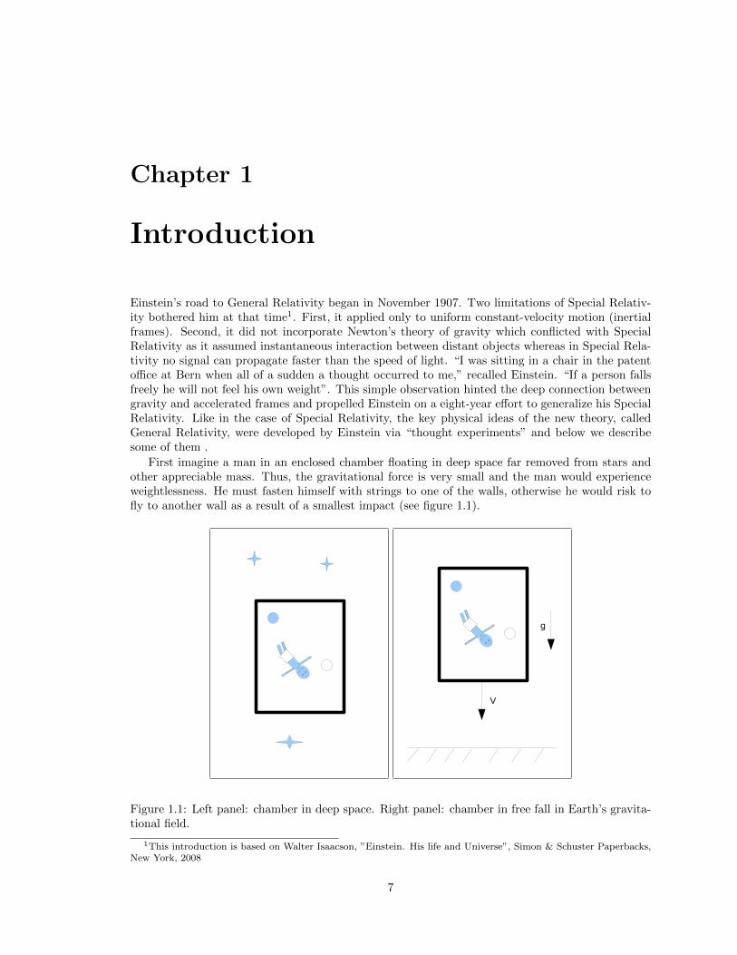
First imagine a man in an enclosed chamber floating in deep space far removed from stars andother appreciable mass. Thus, the gravitational force is very small and the man would experienceweightlessness. He must fasten himself with strings to one of the walls, otherwise he would risk tofly to another wall as a result of a smallest impact (see figure 1.1).
V
g
Figure 1.1: Left panel: chamber in deep space. Right panel: chamber in free fall in Earth’s gravita-tional field.
1This introduction is based on Walter Isaacson, ”Einstein. His life and Universe”, Simon & Schuster Paperbacks,New York, 2008
7

8 CHAPTER 1. INTRODUCTION
Now imagine that the same chamber is released close to earth and now falls freely towards it,accelerating all the time. Again, the man would experience weightlessness just like in deep space(In fact, nowadays this is used to train astronauts). Indeed, as this was discovered by Galileo allobjects freely falling under the Earth’s gravity experience the same acceleration. As the result, theman will not be pressed against the top or bottom walls of the chamber as the chamber acceleratesin exactly the same way as he does (see figure 1.1). Thus, we conclude that accelerated motion canneutralize gravity and in this sense both phenomena are very similar.
Now consider the chamber resting on the ground. The normal reaction force of the groundprevents the chamber from accelerated motion and the man as well as all objects are pressed againstthe floor. Any object lifted from the floor and then released will fall back on the floor (see figure1.2).
Next imagine this chamber in a deep space again but now a rope is attached to one of the walls(the roof) and pulled up with a constant force (acceleration). The man inside the chamber observesthat he and all other objects freely floating inside the chamber before now begin to move withexactly the same acceleration towards the opposite wall (the floor) – just like observed by Galileoin Pisa. Eventually, they all are pressed against the floor. Any object lifted from the floor and thenreleased falls back on the floor (see figure 1.2). All these observations naturally drive the man insideto conclude that the chamber is in gravitational field. He might wonder why the chamber itself isnot in free fall in this gravitational field. Just then, however, he discovers the hook and the rope andcomes to the false conclusion that the chamber is suspended above the ground. This force, howeveris not gravity. It is called inertial force but it’s effects are equivalent to the uniform gravity force.Einstein called this the principle of equivalence: “... it follows that it is impossible to discover byexperiment whether a given system of coordinates is accelerated, or whether ... the observed effectsare due to a gravitational field.”
a=g
g
Figure 1.2: Left panel: accelerated chamber in deep space. Right panel: chamber at rest on groundin Earth’s gravitational field.
The fact that all bodies experience the same acceleration in gravitational field means that theinertial mass equals (proportional) to the gravitational mass (charge). In the second law of Newton,
f = ma,
m is the inertial mass of a body. It describes body’s ability to resist the accelerating effect of force
9
f applied to it. In the Newton’s law of gravity,
f = −GmgM
r3r,
mg is body’s gravitational mass. It describes the intensity of its gravitational interaction withanother body of gravitational mass M . Newton noticed that if
m = mg (1.1)
then the acceleration of the body is independent of its mass
a = −GMr3r.
Thus, all bodies would experience exactly the same acceleration, just like discovered by Galileo.Now we can see that Einstein’s equivalence principle is rooted in the equivalence of inertial andgravitational masses.
These experiments implied that that new relativistic theory of gravity could be constructed viageneralizing Special Relativity in such a way that it deals with not only inertial frames but alsoaccelerated frames. Special Relativity dismissed the notions of absolute space and time. It alsodismissed the notion of absolute motion, that is the motion in absolute space. Only the motionrelative to other physical bodies is considered as meaningful. This equally applies to the motion ofbodies and the motion of reference frames. However, only a particular kind of motion of referenceframes was considered in the original Special Relativity, namely the non-accelerated motion, andhence only a particular kind of reference frames, namely the inertial frames. But why should somereference frames be more special compared to others? If the absolute space does not exist andthus only the relative motion is physically meaningful then whether the motion is accelerated or notshould also be relative. Similarly, there should not be a division on inertial and accelerated referenceframes and more general relativity theory should treat them equally. In particular, the physical lawsmust have the same form (to be covariant) in all reference frames making no distinction betweeninertial and accelerated ones. Hence the name of this new theory: General Relativity.
a=g
g
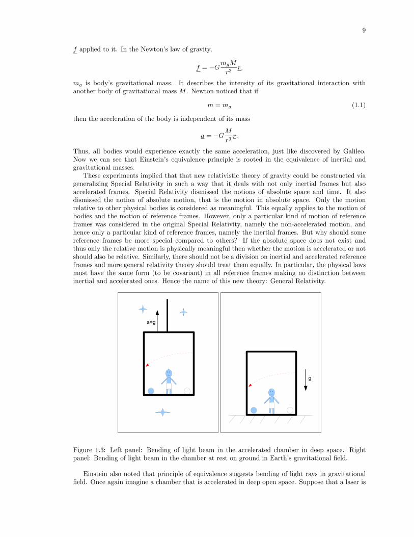
Figure 1.3: Left panel: Bending of light beam in the accelerated chamber in deep space. Rightpanel: Bending of light beam in the chamber at rest on ground in Earth’s gravitational field.
Einstein also noted that principle of equivalence suggests bending of light rays in gravitationalfield. Once again imagine a chamber that is accelerated in deep open space. Suppose that a laser is
10 CHAPTER 1. INTRODUCTION
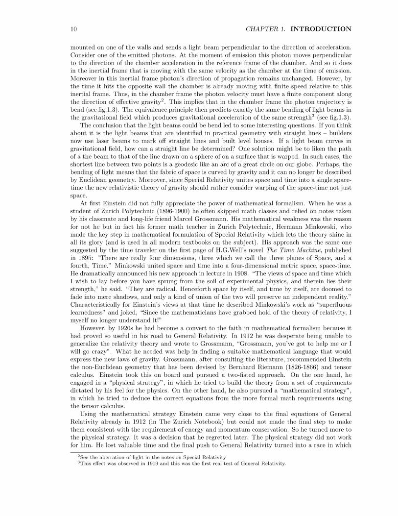
mounted on one of the walls and sends a light beam perpendicular to the direction of acceleration.Consider one of the emitted photons. At the moment of emission this photon moves perpendicularto the direction of the chamber acceleration in the reference frame of the chamber. And so it doesin the inertial frame that is moving with the same velocity as the chamber at the time of emission.Moreover in this inertial frame photon’s direction of propagation remains unchanged. However, bythe time it hits the opposite wall the chamber is already moving with finite speed relative to thisinertial frame. Thus, in the chamber frame the photon velocity must have a finite component alongthe direction of effective gravity2. This implies that in the chamber frame the photon trajectory isbend (see fig.1.3). The equivalence principle then predicts exactly the same bending of light beams inthe gravitational field which produces gravitational acceleration of the same strength3 (see fig.1.3).
The conclusion that the light beams could be bend led to some interesting questions. If you thinkabout it is the light beams that are identified in practical geometry with straight lines – buildersnow use laser beams to mark off straight lines and built level houses. If a light beam curves ingravitational field, how can a straight line be determined? One solution might be to liken the pathof a the beam to that of the line drawn on a sphere of on a surface that is warped. In such cases, theshortest line between two points is a geodesic like an arc of a great circle on our globe. Perhaps, thebending of light means that the fabric of space is curved by gravity and it can no longer be describedby Euclidean geometry. Moreover, since Special Relativity unites space and time into a single space-time the new relativistic theory of gravity should rather consider warping of the space-time not justspace.
At first Einstein did not fully appreciate the power of mathematical formalism. When he was astudent of Zurich Polytechnic (1896-1900) he often skipped math classes and relied on notes takenby his classmate and long-life friend Marcel Grossmann. His mathematical weakness was the reasonfor not he but in fact his former math teacher in Zurich Polytechnic, Hermann Minkowski, whomade the key step in mathematical formulation of Special Relativity which lets the theory shine inall its glory (and is used in all modern textbooks on the subject). His approach was the same onesuggested by the time traveler on the first page of H.G.Well’s novel The Time Machine, publishedin 1895: “There are really four dimensions, three which we call the three planes of Space, and afourth, Time.” Minkowski united space and time into a four-dimensional metric space, space-time.He dramatically announced his new approach in lecture in 1908. “The views of space and time whichI wish to lay before you have sprung from the soil of experimental physics, and therein lies theirstrength,” he said. “They are radical. Henceforth space by itself, and time by itself, are doomed tofade into mere shadows, and only a kind of union of the two will preserve an independent reality.”Characteristically for Einstein’s views at that time he described Minkowski’s work as “superfluouslearnedness” and joked, “Since the mathematicians have grabbed hold of the theory of relativity, Imyself no longer understand it!”
However, by 1920s he had become a convert to the faith in mathematical formalism because ithad proved so useful in his road to General Relativity. In 1912 he was desperate being unable togeneralize the relativity theory and wrote to Grossmann, “Grossmann, you’ve got to help me or Iwill go crazy”. What he needed was help in finding a suitable mathematical language that wouldexpress the new laws of gravity. Grossmann, after consulting the literature, recommended Einsteinthe non-Euclidean geometry that has been devised by Bernhard Riemann (1826-1866) and tensorcalculus. Einstein took this on board and pursued a two-fisted approach. On the one hand, heengaged in a “physical strategy”, in which he tried to build the theory from a set of requirementsdictated by his feel for the physics. On the other hand, he also pursued a “mathematical strategy”,in which he tried to deduce the correct equations from the more formal math requirements usingthe tensor calculus.
Using the mathematical strategy Einstein came very close to the final equations of GeneralRelativity already in 1912 (in The Zurich Notebook) but could not made the final step to makethem consistent with the requirement of energy and momentum conservation. So he turned more tothe physical strategy. It was a decision that he regretted later. The physical strategy did not workfor him. He lost valuable time and the final push to General Relativity turned into a race in which
2See the aberration of light in the notes on Special Relativity3This effect was observed in 1919 and this was the first real test of General Relativity.
11
he almost had been overtaken by a brilliant mathematician, David Hilbert. Luckily for Einstein, hereturned to the mathematical strategy, just in time, and it proved spectacularly successfully. OnNovember 25, 1915 in his lecture “The Field Equations of Gravitation”, Einstein presented the finalresult,
Rνµ − 1/2gνµR = 8πTνµ,
the equation that describes how “matter tells space-time how to curve and the curved space-timetells matter how to move.”
In this course we will not follow all the steps of the complicated route that has lead Einstein toGeneral Relativity. Instead, and along with most modern textbooks, we will pursue the mathematicalstrategy. This is the easiest and the shortest way indeed.
12 CHAPTER 1. INTRODUCTION
Chapter 2
From Euclidean space to surfacesand metric manifolds
2.1 Metric form
2.1.1 The notion of metric form
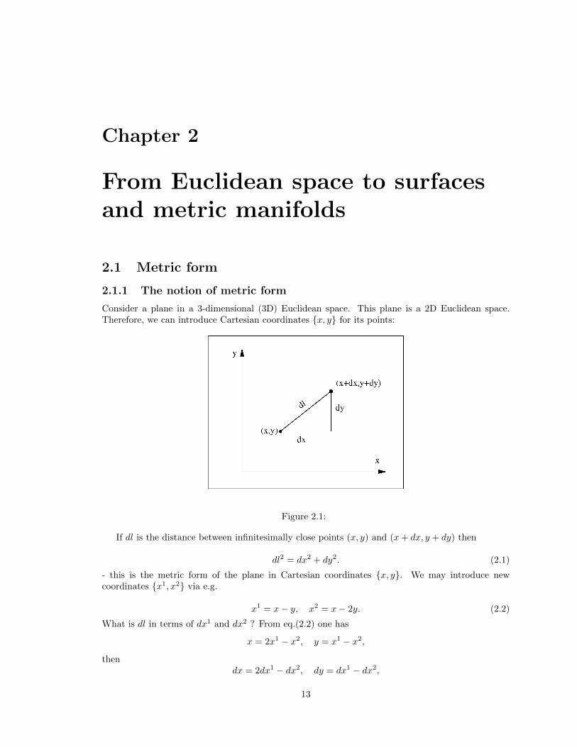
Consider a plane in a 3-dimensional (3D) Euclidean space. This plane is a 2D Euclidean space.Therefore, we can introduce Cartesian coordinates {x, y} for its points:
Figure 2.1:
If dl is the distance between infinitesimally close points (x, y) and (x+ dx, y + dy) then
dl2 = dx2 + dy2. (2.1)
- this is the metric form of the plane in Cartesian coordinates {x, y}. We may introduce newcoordinates {x1, x2} via e.g.
x1 = x− y, x2 = x− 2y. (2.2)
What is dl in terms of dx1 and dx2 ? From eq.(2.2) one has
x = 2x1 − x2, y = x1 − x2,
thendx = 2dx1 − dx2, dy = dx1 − dx2,
13

14CHAPTER 2. FROM EUCLIDEAN SPACE TO SURFACES AND METRIC MANIFOLDS
and finallydl2 = dx2 + dy2 = 5(dx1)2 − 6dx1dx2 + 2(dx2)2
or
dl2 = 5(dx1)2 − 3dx1dx2 − 3dx2dx1 + 2(dx2)2. (2.3)
We may write this as
dl2 =
2∑i=1
2∑j=1
gijdxidxj (2.4)
whereg11 = 5, g12 = g21 = −3, g22 = 2.
For any choice of coordinates the metric form can be written as in eq.(2.4) with gij = gji. Forexample, if x1 and x2 were Cartesian coordinates (just like x and y) then we would have
g11 = 1, g12 = g21 = 0, g22 = 1.
If instead of a 2D Euclidean plane we consider an n-dimensional Euclidean space then we obtaina similar result: the distance between its two infinitesimally close points can be written as
dl2 =
n∑i=1
n∑j=1
gijdxidxj (2.5)
wheregij = gji
for any set of coordinates {xi}, i = 1, 2, ..., n. Coefficients gij of the metric form are often shown ascomponents of a n× n matrix. For example, in the case (2.3)
gij =
(5 −3−3 2
),
and in the case (2.1)
gij =
(1 00 1
),
where it is assumed that x1 = x and x2 = y.
• Einstein summation rule:Any index appearing once as a lower index and once as an upper index of the same indexed object
or in the product of a number of indexed objects stands for summation over this index. Such indexis called a dummy index. Indexes which are not dummy are called free indexes.
According to this rule we can rewrite eq.(2.5) in a more concise form:
dl2 = gijdxidxj . (2.6)
This rule allows to simplify expressions involving multiple summations. Here are some more exam-ples:
1. aibi stands for
∑ni=1 aib
i; here i is a dummy index;
2. aibi stands for a product of ai and bi where i can have any value between 1 and n; here i is afree index.
3. aibkij stands for
∑ni=1 aib
kij ; here k and j are free indexes and i is a dummy index;
4. ai ∂f∂xi stands for∑ni=1 a
i ∂f∂xi ; thus, index i in the partial derivative ∂
∂xi is treated as a lowerindex;

2.1. METRIC FORM 15
2.1.2 Metric forms of surfaces:
For any smooth surface in Euclidean space the distance between its any two infinitesimally closepoints can be found in terms of coordinates introduced on the surface. For example, consider asphere of radius r in 3D Euclidean space. This is a 2D surface and one needs two coordinates tomark its points. Introduce the usual spherical coordinates {θ, φ}.
Figure 2.2:
Then for the Cartesian coordinates {x, y, z} shown in the figure x = r sin θ cosφ,y = r sin θ sinφ,z = r cos θ
.
This gives us dx = r cos θ cosφdθ − r sin θ sinφdφ,dy = r cos θ sinφdθ + r sin θ cosφdφ,dz = −r sin θdθ
and
dl2 = dx2 + dy2 + dz2 = ... = r2dθ2 + r2sin2θdφ2. (2.7)
Thus,
gij =
(r2 00 r2 sin2 θ
)where we assume that x1 = θ and x2 = φ.
• Locally Cartesian coordinates:
It is impossible to introduce Cartesian coordinates for the whole sphere, that is such two coor-dinates x1 and x2 that
dl2 = (dx1)2 + (dx2)2
everywhere on the sphere (a sphere is not like a plane). However, there exist so-called locallyCartesian coordinates.

16CHAPTER 2. FROM EUCLIDEAN SPACE TO SURFACES AND METRIC MANIFOLDS
Take some point of the sphere, denote it as A. Suppose its spherical coordinates are θa and φa.Near A introduce new coordinates {
x1 = r(θ − θa)x2 = r sin θa(φ− φa)
.
Then {dx1 = rdθdx2 = r sin θadφ
,
and {dθ = dx1/rdφ = dx2/r sin θa
.
Substitute these into eq.(2.7) to obtain the metric form
dl2 = (dx1)2 +
(sin θ
sin θa
)2
(dx2)2.
At the point A this becomesdl2 = (dx1)2 + (dx2)2.
Thus, near point A the metric form is the same as the metric form of a 2D Euclidean space withCartesian coordinates {xi}. Because of this property, the sphere is called ”locally Euclidean” or”Riemannian”. (All smooth surfaces in Euclidean space are locally Euclidean.)
2.1.3 Lengths of curves
Let {xi} be some arbitrary (curvilinear) coordinates in n-dimensional Euclidean space and xi = xi(λ)be a curve in the space. (λ is the curve parameter; one can view it as a coordinate introduced onlyfor the points of the curve).
Figure 2.3:
The length of the curve between its any two points, A and B, is given by
∆l =
B∫A
dl =
B∫A
(gijdxidxj)1/2 =
λB∫λA
(gijdxi
dλ
dxj
dλ
)1/2
dλ. (2.8)
2.1.4 Coordinate transformations:
Introduce arbitrary new coordinates {xi′} whose coordinate lines may be curved. xi′
are functionsof the old coordinates xk:
xi′
= xi′(xk).
Inversely, xk are functions of xi′:
xk = xk(xi′).
2.2. VECTORS, BASES, AND COMPONENTS OF VECTORS 17
Then
dl2 = gijdxidxj = gi′j′dx
i′dxj′, (2.9)
where
gij =∂xl
′
∂xi∂xm
′
∂xjgl′m′ , and gi′j′ =
∂xl
∂xi′∂xm
∂xj′glm. (2.10)
Eq.(2.10) is the transformation law for the components of the metric form.If {xi} are Cartesian then
glm =
{1 if l = m0 if l 6= m
(2.11)
and the second equation in eq.(2.10) reduces to
gi′j′ =
n∑l=1
∂xl
∂xi′∂xl
∂xj′. (2.12)
2.2 Vectors, bases, and components of vectors
In Euclidean geometry vectors are defined as straight arrows. The magnitude of a vector is thelength of the arrow. We denote it as |a|.
2.2.1 Coordinate bases
Let {xi} be Cartesian coordinates of n-dimensional Euclidean space. Let ei be the unit vectorspointing in the direction of the xi-coordinate axis. The set of all n vectors ei at any point of thespace forms a vector basis at this point, the Cartesian basis. If
a = aiei
then ai are the components of a in this basis. Vector
r = xkek. (2.13)
whose base coincides with the origin of the coordinate system and whose tip coincides with the pointwith coordinates xk is called the position vector of this point.
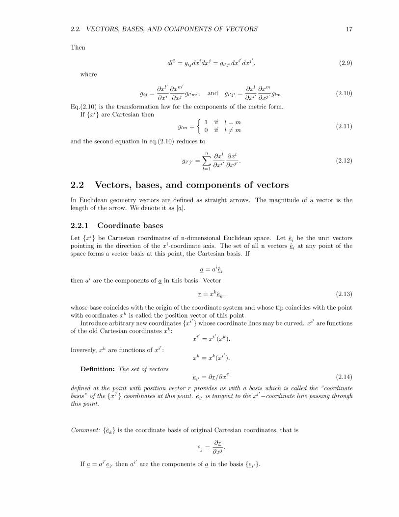
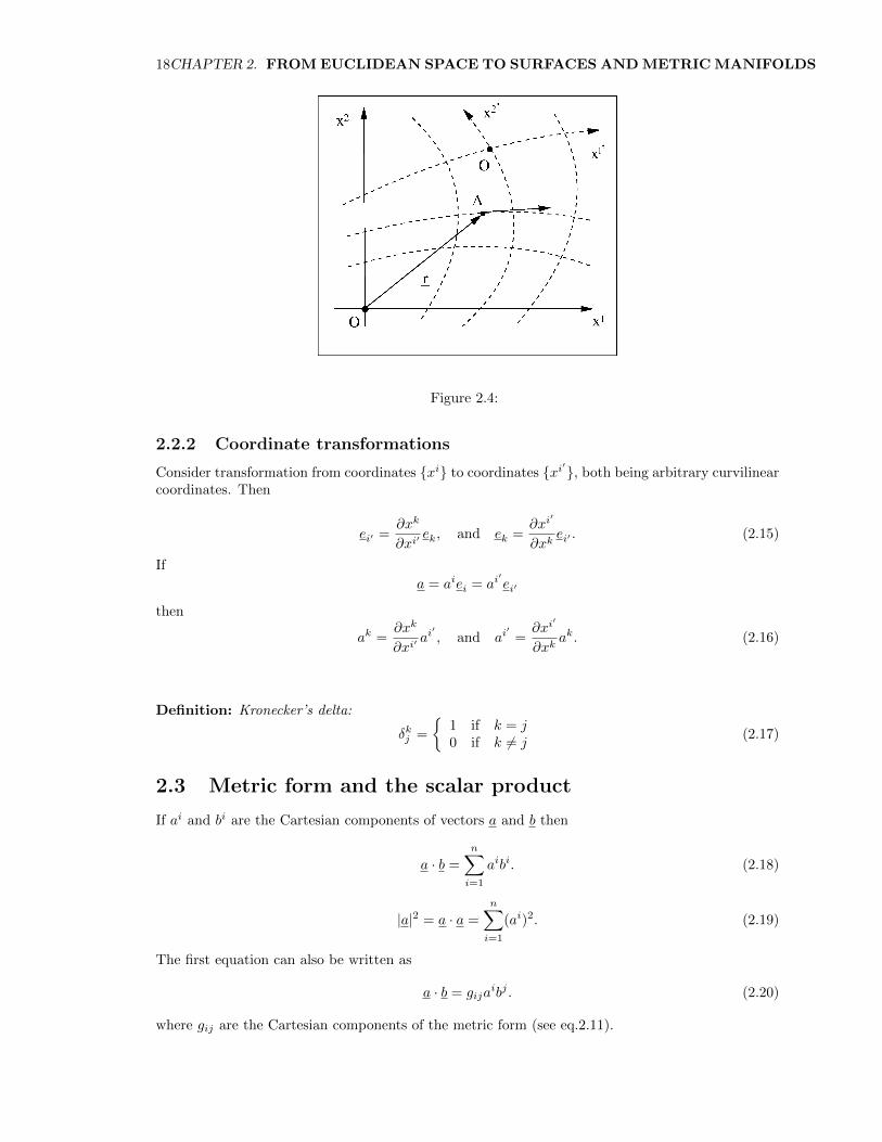
Introduce arbitrary new coordinates {xi′} whose coordinate lines may be curved. xi′are functions
of the old Cartesian coordinates xk:xi
′= xi
′(xk).
Inversely, xk are functions of xi′:
xk = xk(xi′).
Definition: The set of vectorsei′ = ∂r/∂xi
′(2.14)
defined at the point with position vector r provides us with a basis which is called the ”coordinatebasis” of the {xi′} coordinates at this point. ei′ is tangent to the xi
′−coordinate line passing throughthis point.
Comment: {ek} is the coordinate basis of original Cartesian coordinates, that is
ej =∂r
∂xj.
If a = ai′ei′ then ai
′are the components of a in the basis {ei′}.
18CHAPTER 2. FROM EUCLIDEAN SPACE TO SURFACES AND METRIC MANIFOLDS
Figure 2.4:
2.2.2 Coordinate transformations
Consider transformation from coordinates {xi} to coordinates {xi′}, both being arbitrary curvilinearcoordinates. Then
ei′ =∂xk
∂xi′ek, and ek =
∂xi′
∂xkei′ . (2.15)
If
a = aiei = ai′ei′
then
ak =∂xk
∂xi′ai
′, and ai
′=∂xi
′
∂xkak. (2.16)
Definition: Kronecker’s delta:
δkj =
{1 if k = j0 if k 6= j
(2.17)
2.3 Metric form and the scalar product
If ai and bi are the Cartesian components of vectors a and b then
a · b =
n∑i=1
aibi. (2.18)
|a|2 = a · a =
n∑i=1
(ai)2. (2.19)
The first equation can also be written as
a · b = gijaibj . (2.20)
where gij are the Cartesian components of the metric form (see eq.2.11).
2.4. GEODESICS AND THE VARIATIONAL PRINCIPLE 19
In fact, if ai′
and bi′
are the components of a and b and gi′j′ are the components of the metricform in the coordinate basis of any other coordinate system we still have
a · b = gi′j′ai′bj
′. (2.21)
Thus, expression (2.20) for the scalar product of two vectors is invariant under coordinate transfor-mations(!)
If gij are the components of the metric form in some coordinate system and {ei} is the coordinatebasis of this system then
gij = ei · ej . (2.22)
Consider an infinitesimally small vector dx connecting points with coordinates xi and xi + dxi.The components of dx in the coordinate basis are dxi. The magnitude of dx is the distance dlbetween the points. Then from the invariant expression eq.(2.21) one has
dl2 = dx · dx = gijdxidxj (2.23)
in agreement with eq.(2.6)
2.4 Geodesics and the variational principle
2.4.1 Euler-Lagrange Theorem
Consider the functional
lAB =
λB∫λA
L(xk, xk)dλ (2.24)
where xk = xk(λ) (k = 1, 2, ..., n) are functions of λ and xk = dxk/dλ.The functions which extremise lAB and satisfy the boundary conditions
xk(λA) = xkA, xk(λB) = xkB (2.25)
are solutions of the following ODEs
d
dλ
∂L
∂xk− ∂L
∂xk= 0 (k = 1, 2, ..., n) (2.26)
These ODEs are known as Euler-Lagrange equations.
2.4.2 Geodesics
Consider an n-dimensional Euclidean space or even a smooth surface in a higher dimensional Eu-clidean space. Let xi, i = 1, 2, ..., n be some arbitrary coordinates in this space or surface and gijare the corresponding components of the metric form.
Consider a curve xk = xk(λ) connecting points A and B with coordinates xkA and xkB , that is
xk(λA) = xkA, xk(λB) = xkB .
20CHAPTER 2. FROM EUCLIDEAN SPACE TO SURFACES AND METRIC MANIFOLDS
The distance between A and B along this curve is
lAB =
λB∫λA
L(xk, xk)dλ
where Lagrangian L isL(xk, xk) = [gij x
ixj ]1/2. (2.27)
Note that in general gij = gij(xk).
Definition: Curves that extremise distances between all its points are called geodesics.
From the Euler-Lagrange theorem it follows that geodesics are solutions of the Euler-Lagrangeequations with Lagrangian (2.27). Instead of the Lagrangian (2.27) one can also use the Lagrangian
L(xk, xk) = gij xixj . (2.28)
This will result in the same curves but with different parametrization. Namely, λ will be a normalparameter, that is such a parameter that
dλ = adl,
where a =const and l is the length of the geodesic (as measured from an arbitrary point of thegeodesic).
2.4.3 Examples of geodesics:
•Euclidean space:
If xk are Cartesian coordinates then the Lagrangian (2.28) reads
L =
n∑i=k
(xk)2
and the corresponding Euler-Lagrange equations reduce to
dxk
dλ= 0,
The solutions of these equations,xk(λ) = akλ+ bk,
describe straight lines.
•2D sphere in a 3D Euclidean space:
Consider a sphere of radius r with spherical coordinates {θ, φ}. Then the Lagrangian (2.28)reads
L = r2(θ2 + sin2 θφ2)
2.4. GEODESICS AND THE VARIATIONAL PRINCIPLE 21
and the corresponding Euler-Lagrange equations reduce to
ddλ
(sin2 θ dφdλ
)= 0
ddλ
(dθdλ
)− sin θ cos θ
(dφdλ
)2= 0.
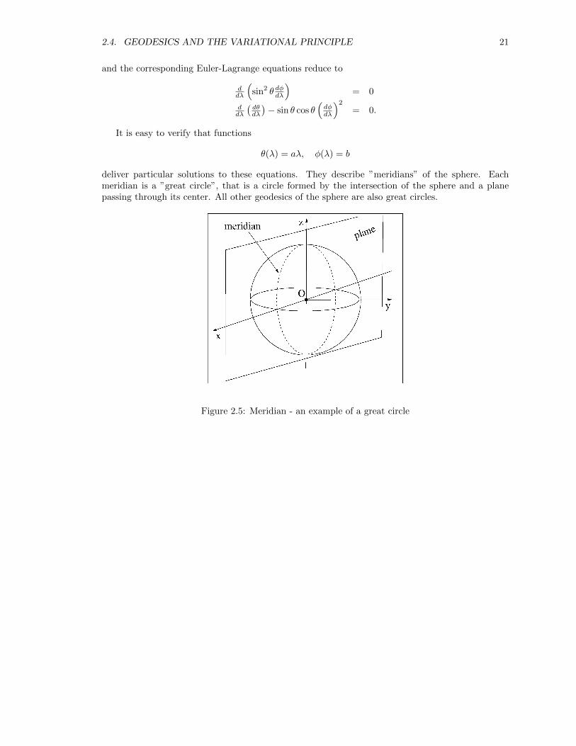
It is easy to verify that functions
θ(λ) = aλ, φ(λ) = b
deliver particular solutions to these equations. They describe ”meridians” of the sphere. Eachmeridian is a ”great circle”, that is a circle formed by the intersection of the sphere and a planepassing through its center. All other geodesics of the sphere are also great circles.
Figure 2.5: Meridian - an example of a great circle
22CHAPTER 2. FROM EUCLIDEAN SPACE TO SURFACES AND METRIC MANIFOLDS
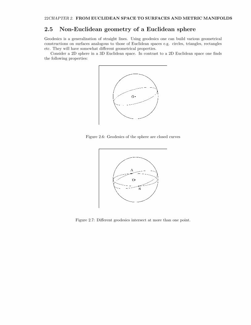
2.5 Non-Euclidean geometry of a Euclidean sphere
Geodesics is a generalization of straight lines. Using geodesics one can build various geometricalconstructions on surfaces analogous to those of Euclidean spaces e.g. circles, triangles, rectanglesetc. They will have somewhat different geometrical properties.
Consider a 2D sphere in a 3D Euclidean space. In contrast to a 2D Euclidean space one findsthe following properties:
Figure 2.6: Geodesics of the sphere are closed curves
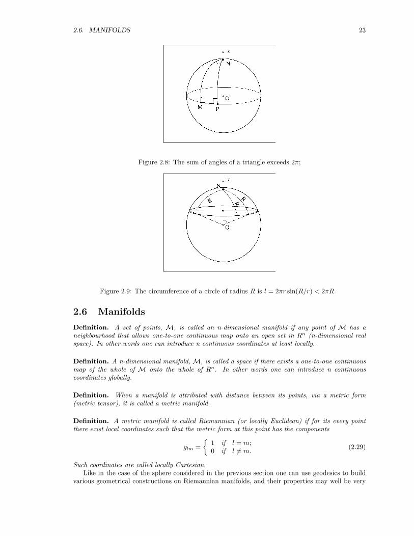
Figure 2.7: Different geodesics intersect at more than one point.
2.6. MANIFOLDS 23
Figure 2.8: The sum of angles of a triangle exceeds 2π;
Figure 2.9: The circumference of a circle of radius R is l = 2πr sin(R/r) < 2πR.
2.6 Manifolds
Definition. A set of points, M, is called an n-dimensional manifold if any point of M has aneighbourhood that allows one-to-one continuous map onto an open set in Rn (n-dimensional realspace). In other words one can introduce n continuous coordinates at least locally.
Definition. A n-dimensional manifold, M, is called a space if there exists a one-to-one continuousmap of the whole of M onto the whole of Rn. In other words one can introduce n continuouscoordinates globally.
Definition. When a manifold is attributed with distance between its points, via a metric form(metric tensor), it is called a metric manifold.
Definition. A metric manifold is called Riemannian (or locally Euclidean) if for its every pointthere exist local coordinates such that the metric form at this point has the components
glm =
{1 if l = m;0 if l 6= m.
(2.29)
Such coordinates are called locally Cartesian.Like in the case of the sphere considered in the previous section one can use geodesics to build
various geometrical constructions on Riemannian manifolds, and their properties may well be very

24CHAPTER 2. FROM EUCLIDEAN SPACE TO SURFACES AND METRIC MANIFOLDS
different from those in Euclidean geometry.
Definition. A Riemannian manifold is called a Euclidean space if there exist global coordinates,called Cartesian, such that the metric form has components (2.29) at every point of the manifold.
A 2-dimensional sphere in a 3-dimensional Euclidean space is a 2-dimensional Riemannian manifoldbut not a Euclidean space. A 2-dimensional plane in a 3-dimensional Euclidean space is a 2-dimensional Euclidean space. All smooth surfaces in a Euclidean space are Riemannian manifolds.
A manifold is not necessarily a surface in a Euclidean or any other space. The spacetime ofGeneral Relativity is an example of such manifold.
2.7 Vectors as operators
2.7.1 Basic idea
Vectors defined as straight arrows do not suit surfaces and manifolds. Such straight arrows cannotbelong to curved surfaces and, at most, can only be tangent to them, unless they are infinitesimallysmall.
Vectors defined as directed bits of surface geodesics do not allow to introduce meaningful opera-tions of addition and multiplication by real number, unless their are infinitesimally small and, thus,indistinguishable from straight arrows tangent to the surface.
Cartan proposed to define vectors as directional derivatives. Consider a n-dimensional surfacewith coordinates {xi} and a particle moving over the surface. The particle coordinates are functionsof time:
xi = xi(t). (2.30)
These equations describe a curve on the surface, the particle trajectory. t plays the role of itsparameter. The derivatives
vi =dxi
dt(2.31)
have the meaning of velocity components. Consider the differential operator
d
dt= vi
∂
∂xi, (2.32)
called the directional derivative along the curve (2.30). Note that vi are components of the operatord/dt in the basis of partial derivatives ∂/∂xi. Hence, the idea to identify the velocity vector withthis directional derivative and treat the partial derivatives and its local coordinate basis:
v =d
dt, ei =
∂
∂xi. (2.33)
Then eq.(2.32) reads
v = viei, (2.34)
Addition and multiplication of Cartan’s vectors is defined via eq.2.32. That is
c = a+ b if ci = ai + bi;
and
a = αb if ai = αbi.
The set of all vectors defined this way at any particular point of the surface form an n-dimensionalvector space associated with this point.

2.7. VECTORS AS OPERATORS 25
2.7.2 Coordinate transformations
Introduce new coordinates, {xi′}. According to the chain rule:
∂
∂xi′=∂xk
∂xi′∂
∂xkand
∂
∂xk=∂xi
′
∂xk∂
∂xi′.
or,
ei′ =∂xk
∂xi′ek, and ek =
∂xi′
∂xkei′ ,
exactly as in eq.(2.15). Then from
v = viei = vi′ei′ .
one has
vk =∂xk
∂xi′vi
′, and vi
′=∂xi
′
∂xkvk, (2.35)
just like in eq.(2.16). Thus, the new definition of vectors as operators leads to the same transforma-tion laws for their components as before. Note that neither the trajectory nor its parameter t areeffected by such transformation. Thus, the directional derivative v = d/dt is not effected either. Itis completely independent on the choice coordinates and exists even if no coordinates are introducedaltogether.
2.7.3 Magnitudes of vectors and the scalar product
Let v and w be two Cartan vectors (operators). Because of the transformation law (2.35) the quantitygijv
iwj remains invariant under coordinate transformations (such quantities are called scalars.) Thiscan still be called the scalar product of v and w
v · w = gijviwj .
Moreover, gijvivj , provides meaningful definition for the magnitude v = |v| of vector v:
|v|2 = gijvivj .
Indeed, consider the infinitesimal displacement vector of our particle,
dx = vdt.
Its componentsdxi = vidt
are the differences in coordinates of the two points on the particle trajectory separated by time dt.The distance between these points point is given by
dl2 = gijdxidxj = (gijv
ivj)dt2 = v2dt2.
Thus, we havedl = vdt
as usual.
In fact, none of the properties of Euclidean vectors introduced as arrows is lost by Cartan’svectors introduced as operators.
26CHAPTER 2. FROM EUCLIDEAN SPACE TO SURFACES AND METRIC MANIFOLDS
Chapter 3
Tensors
Tensors are used not only in the Theory of Relativity but also in many fields of Newtonian physics,sometimes without proper introduction.
3.1 Tensors as operators
Consider an n-dimensional manifold. Let P be a point of the manifold. Denote as Tp the set of allvectors defined at P. Tp is an n-dimensional vector space (see Sec.1.7.1)
3.1.1 1-forms as operators acting on vectors
Definition. A 1-form q defined at P is a linear scalar operator acting on vectors from Tp. That is
1. q : Tp → R;
2. For any v, u ∈ Tp and a, b ∈ R
q(av + bu) = aq(v) + bq(u). (3.1)
The set of all 1-forms defined at P is denoted as T ∗p . This is an n-dimensional vector space with
1. Zero-element 0 such that0(u) = 0 for any u ∈ Tp;
2. Operation of addition:q = p+ w if for any u ∈ Tp
q(u) = p(u) + w(u); (3.2)
3. Operation of multiplication:q = ap if for any u ∈ Tp
q(u) = ap(u). (3.3)
To stress that 1-form q is an operator it is often shown as
q( )
where the space inside the brackets is a slot to be filled with a vector.
27

28 CHAPTER 3. TENSORS
Examples of 1-forms:
• To any vector v ∈ Tp there corresponds a 1-form v introduced via the scalar product operationas follows
v(u) = v · u for any u ∈ Tp. (3.4)
This 1-form is called ”dual” to the vector v. The condition (3.1) is satisfied because
v · (au+ bw) = a(v · u) + b(v · w).
• Gradient of a scalar function.
Let f be a scalar function defined on the manifold. The 1-form df such that for any infinites-imally small vector dx from Tp
df(dx) = df (3.5)
is called the gradient of f at point P.
Figure 3.1:
Since df = (∂f/∂xi)dxi we have
df(dx) =∂f
∂xidxi.
This suggests that for any vector u
df(u) =∂f
∂xiui. (3.6)
The expression on the right is indeed a scalar (a number which the same for all coordinates):
∂f
∂xiui =
∂f
∂xi
(∂xi
∂xj′uj
′)
=
(∂f
∂xi∂xi
∂xj′
)uj
′=
∂f
∂xj′uj
′.
3.1.2 Vectors as operators acting on 1-forms
One can associate with any vector u ∈ Tp a linear scalar operator acting on 1-forms from T ∗p via
u(q) = q(u) ≡< u, q > (3.7)
From eqs.(3.2) and (3.3) it follows that indeed
u(ap+ bq) = au(p) + bu(q).
To stress this role of vectors they are often shown like
u( )
where the space inside the brackets is a slot to be filled with a 1-form.

3.1. TENSORS AS OPERATORS 29
3.1.3 Tensors as operators acting on vectors and 1-forms
Definition. An(lm
)-type tensor defined at point P is a linear scalar operator with l slots for 1-forms
from T ∗p and m slots for vectors from Tp. Such tensor can also be called as l-times contravariantand m-times covariant. The total number of slots, r = l +m, is called the rank of the tensor.
Thus,
1. Any vector is a(10
)-type tensor;
2. Any 1-form is a(01
)-type tensor;
3. If, for example, M( , ) is(11
)-type tensor with the first slot reserved for 1-forms then
•M(q, u) ∈ R;
•M(ap+ bq, u) = aM(p, u) + bM(q, u);
•M(p, au+ bv) = aM(p, u) + bM(p, v);
The set of all(lm
)-type tensors defined at point P is an nr-dimensional vector space with
1. Zero element O such that
O(u, . . . , q) = 0 for any l vectors from Tp and m 1-forms from T ∗p ;
2. Operation of addition
S = T +K if for any l vectors from Tp and m 1-forms from T ∗p
S(u, . . . , q) = T (u, . . . , q) +K(u, . . . , q); (3.8)
3. Operation of multiplication by real numbers
S = aT, where a ∈ R, if for any l vectors from Tp and m 1-forms from T ∗p
S(u, . . . , q) = aT (u, . . . , q); (3.9)
3.1.4 Metric tensor
Definition. A(02
)-type tensor g( , ) such that for any two vectors v, u ∈ Tp
g(v, u) = v · u (3.10)
is call the metric tensor.
Notice that the metric tensor and the one-form v dual to the vector v (see Sec.2.1.1) are relatedvia
v( ) = g(v, ). (3.11)
Indeed, this ensures thatv(u) = g(v, u) = v · u.
Later on we will describe a relationship between the metric tensor and the metric form

30 CHAPTER 3. TENSORS
3.1.5 Constructing higher rank tensors via outer multiplication of vectorsand 1-forms
The following examples explain the operation of outer multiplication. ⊗ is the symbol of thisoperation. Here v, u etc. are vectors from Tp, and p, q etc. are 1-forms from T ∗p .
• Example
F ( , ) = u( )⊗ v( )
is a(20
)-type tensor such that for any p, q
F (p, q) = u(p)v(q);
• Example
S( , ) = q( )⊗ v( )
is a(11
)-type tensor such that for any p, u
S(u, p) = q(u)v(p);
• Example
D( , , ) = q( )⊗ v( )⊗ t( )
is a(12
)-type tensor such that for any p, u, s
D(u, p, s) = q(u)v(p)t(s);
etc.
3.2 Bases and components of tensors
3.2.1 Induced basis of 1-forms
Let {ei}ni=1 be a basis in Tp. Then for any u ∈ Tp
u( ) = uiei( ). (3.12)
ui are the components of u in this basis. Note that i is an upper index.Let {wi}ni=1 be a basis in T ∗p . Then for any q ∈ T ∗p
q( ) = qiwi( ), (3.13)
where qi are the components of q in this basis. Note that i is a lower index in qi. This is to makeclear that we are dealing with the components of a 1-form but not a vector. In order to utilise theEinstein summation rule in equations like eq.(3.13) we are then forced to use upper indices for thebasis 1-forms wi.
From eqs.(3.12,3.13) one has
wi(u) = ujwi(ej);ei(q) = qjei(w
j);q(u) = qiu
jwi(ej).(3.14)
Definition. The basis {wi} is called induced by the basis {ei} if
wi(ej) = δij . (3.15)
3.2. BASES AND COMPONENTS OF TENSORS 31
Then eqs.(3.14) simplify so that we have
wi(u) = ui;ei(q) = qi;q(u) = qiu
i.(3.16)
Such simplifications is the main reason for using induced bases of 1-forms.
3.2.2 Induced bases of tensors
Induced bases of tensors are introduced for the same reason (simplicity). The following examplesexplain how these bases are constructed:
(a) The induced basis of(11
)-type tensors with the first slot intended for 1-forms is {ei ⊗ wj},
where {wi} is the induced basis of 1-forms.
If F ( , ) is such a tensor and F ij are its components in this basis, then
F ( , ) = F ij ei( )⊗ wj( ); (3.17)
F ij = F (wi, ej); (3.18)
F (q, u) = F ijqiuj . (3.19)
(b) The induced basis of(02
)-type tensors is {wi ⊗ wj}. If g( , ) is such a tensor and gij are its
components in this basis then
g( , ) = gijwi( )⊗ wj( ); (3.20)
gij = g(ei, ej); (3.21)
g(u, v) = gijuivj . (3.22)
etc.
3.2.3 Index notation of tensors
The number and position of indexes of tensor components reveal all the general information abouttensors as operators. For example if tensor T has components T i kj l this immediately tells us that
1. T is a 4th rank tensor;
2. T is a(22
)-type tensor;
3. Its 1st and 3rd slots are for 1-forms whereas its 2nd and 4th slots are for vectors. That is
T ( , , , ) = T i kj lei( )⊗ wj( )⊗ ek( )⊗ wl( )
Because of this nice property it is a custom to introduce tensors simply by showing their components.Hence, it is perfectly OK to say
”Let us consider tensor T i kj l”

32 CHAPTER 3. TENSORS
3.2.4 Coordinate bases
In Section 1.7.1 we introduced the coordinate basis
{∂/∂xi} i = 1, . . . , n
of vectors ( {∂r/∂xi} in the old fashion notation; see also Sec.1.2.1). The corresponding inducedbases of other tensors are also called coordinate. The coordinate basis of 1-forms is denoted as
{dxi} i = 1, . . . , n.
The coordinate basis of(02
)-type tensors is then
{dxi⊗ dx
j} i, j = 1, . . . , n
etc.
3.2.5 Coordinate components of df
If df is the gradient of the scalar function f then
df =∂f
∂xidx
i. (3.23)
Thus, ∂f/∂xi are the components of df in the coordinate basis of the coordinates {xi}.
3.2.6 Metric form and metric tensor
The metric form
dl2 = gijdxidxj (3.24)
gives us the distance, dl, between the point xi and the point xi + dxi. Consider the infinitesimallysmall vector
dx = dxi∂
∂xi.
If g( , ) is the metric tensor than
dx · dx = g(dx, dx) = gijdxidxj , (3.25)
where
gij = g
(∂
∂xi,∂
∂xj
)are the coordinate components of the metric tensor. Comparison of eq.(3.24) with eq.(3.25) showsthat
the components gij of the metric form are nothing else but the components of the metric tensorin the coordinate basis.
3.3 Basic tensor operations and tensor equations
Definition. Operations with tensors which produce other tensors are call tensor operations.
All such operations can be introduced without making use of bases and components of tensors.However, in this section we only describe the effect they have on components of tensors. In fact,this is a very concise and fully comprehensive way of describing tensor operations. Keep in mindthat what is shown below are just examples involving tensors of particular types. Generalisation,however, is very straightforward.
3.3. BASIC TENSOR OPERATIONS AND TENSOR EQUATIONS 33
1. Addition:
Cij = Aij +Bij (3.26)
when tensor C is a sum of tensors A and B;
2. Multiplication by a real number:
Cijk = aAijk (3.27)
when tensor C is a product of real number a and tensor A;
3. Outer multiplication:
T ijkl = DijBkl (3.28)
when T is the outer product of D and B (T = D ⊗B);
4. Contraction of a single tensor:
Sij = T illj (3.29)
when S is the result of contracting T over its second upper and first lower indexes (l is adummy index);
5. Contraction of two tensors:
T ij = DilBlj (3.30)
when T is the result of contraction D and B over the 2nd upper index of D and the first lowerindex of B (l is a dummy index);
Equations relating different tensors by means of tensor operations are called tensor equations.Thus, equations 3.26-3.30 are examples of tensor equations. All tensor equations satisfy the followingsimple formal rules:
1. All terms of tensor equations must have the same number and positions of freeindexes. Thus, for example, if i is an upper free index in one of the terms then it must be
an upper free index in all other terms.
Examples:
Sij = T ikj + P ij
is not a proper tensor equation whereas
Sij = T ikkj + P ij
is.
2. The order of free indexes is not important, so
Sij = T ikkj +D ij
is still OK.
3. Also remember not to write a lower index just below an upper index because this makes theorder of slots ambiguous. That is
Sij = T ikkj + P ij
is not OK.
34 CHAPTER 3. TENSORS
• Theorem
If a tensor equation involves m indexed objects and we know that
m− 1 of them are tensors then the remaining one is also a tensor. (3.31)
For example, if T ikl and ui are tensors and
T ikl = uiBkl
then Bkl is also a tensor. This theorem is proved using the transformation law of components oftensors.
3.4 Basis transformation
Here we study the way the components of tensors transform as the result of the transformationof the vector basis {ei} and, hence, the transformations of the induced bases of all other tensorstriggered by this transformation of the vector basis. The old style definition of tensors was basedon this transformation law. As before, we shell use ”dash” to indicate new bases and componentsof tensors.
Any vector of the new vector basis is a linear combination of the vectors of the old vector basis.Hence,
ek′ = Aik′ei. (3.32)
Aik′ is the transformation matrix (not a tensor). Similarly,
ek = Ai′
k ei′ . (3.33)
The transformation matrix Ai′
k is inverse to Aik′ , that is
Ai′
kAkj′ = δi
′
j′ and Ai′
kAji′ = δjk. (3.34)
If {ei = ∂∂xi } and {ei′ = ∂
∂xi′ } are the coordinate bases of coordinates {xi} and {xi′} respectivelythen
Ai′
k =∂xi
′
∂xkand Aji′ =
∂xj
∂xi′. (3.35)
3.4.1 Transformation of induced bases
The corresponding transformation of the induced basis of 1-forms is
wk′
= Ak′
i wi and wk = Aki′w
i′ . (3.36)
Given new bases of vectors and 1-forms one can construct induced bases of all higher rank tensors.For example
ei′ ⊗ wj′
= Aki′Aj′
l ek ⊗ wl; (3.37)
ei′ ⊗ ej′ = Aki′Alj′ek ⊗ el; (3.38)
wi′⊗ wj
′= Ai
′
kAj′
l wk ⊗ wl. (3.39)
3.5. THE OPERATIONS OF RAISING AND LOWERING INDEXES OF TENSORS 35
3.4.2 Transformation of components
Given the new basis (new induced basis) one can find the components of any tensor in this new basisand relate them to the original components in the old basis.
Vectors:
ui = Aik′uk′ and ui
′= Ai
′
k uk; (3.40)
1-forms:
qi = Ak′
i qk′ and qi′ = Aki′qk; (3.41)
Higher rank tensors:
General rule: Each upper index is treated as a vector index
and each lower index as an index of a 1-form. (3.42)
For example,
T i′
j′ = Ai′
kAlj′T
kl and T ij = Aik′A
l′
j Tk′
l′ (3.43)
3.5 The operations of raising and lowering indexes of tensors
δij can be considered as a tensor because it satisfies the tensor transformation law, eq.3.42. Indeed,
Aik′Al′
j δk′
l′ = Ail′Al′
j = δij .
Now suppose we are dealing with a metric manifold. Consider the tensor equation
gijgjk = δik, (3.44)
where gjk is the metric tensor. Since both gjk and δjk are tensors so must be gij (see eq.3.31). Thistensor is also called the metric tensor. This makes perfect sense because gij is uniquely defined bygij .
We already know that the metric tensor allows to relate vectors and 1-forms (see eq.3.11):
u( ) = g(u, ).
In components this reads
ui = gijuj . (3.45)
Given eq.3.44 we invert eq.3.45 to find
ui = gijuj . (3.46)
Thus, the metric tensor allows to define a one-to-one relationship (map) between vectorsand 1-forms. Now we can interpret u as a first rank tensor which can be representedeither as a vector, u, or a 1-form, u.
Often, the components ui are called the covariant components of u and ui the contravariantcomponents of u. This is because the transformation law for ui is the same as the one for the basisvectors (they covary) and it is different for ui:
ui′ = Aji′uj and ei′ = Aji′ej but ui′
= Ai′
j uj .
36 CHAPTER 3. TENSORS
Similarly, the metric tensor is used to unify all tensors of the same rank. For example, if
T ij = gjkTik
T ji = gikT
kj
Tij = gikgjlTkl
(3.47)
then T ij , Tij , Tij , and T j
i are different representations of the same tensor T . For this reasonthe operations like (3.45-3.47) are called rising and lowering indexes of a tensor.
• In the operation of contraction it does not matter which of the dummy indexes is lower andwhich is upper. For example,
T ikuk = T ikuk. (3.48)
• The vector-gradient of a scalar function f , ∇f , if defined as
∇if = gijdfj = gij∂f
∂xj. (3.49)
Thus, df and ∇f represent the same 1st rank tensor called the gradient of f .
3.6 Symmetric and antisymmetric tensors
In many applications we deal with so-called symmetric and antisymmetric tensors. Here we explainwhat they are by example.
3.6.1 Symmetry with respect to a pair of indexes
Tensor T ijk is called symmetric with respect to i and j if
T ijk = T jik. (3.50)
When any of the indexes of T is lowered the symmetry is preserved. That is
T ijk = T jikT ijk = T i
j k
T kij = T k
ji .
(3.51)
3.6.2 Antisymmetry with respect to a pair of indexes
Tensor T ijk is called antisymmetric with respect to i and j if
T ijk = −T jik. (3.52)
When any of the indexes of T is lowered the symmetry is preserved. That is
T ijk = −T jikT ijk = −T i
j k
T kij = −T k
ji .
(3.53)
It is easy to show that if T ijk is symmetric with respect to i and j and Fij is antisymmetric withrespect to i and j then
T ijkFij = 0. (3.54)
Indeed,T ijkFij = −T ijkFji = −T jikFji = −T ijkFij ,
where the first equality is due to the antisymmetry of Fij , the second one is due to symmetry ofT ijk and the third one stands because we simply rename dummy indexes. Next we obtain
2T ijkFij = 0,
from which eq.3.54 follows.
Chapter 4
Geometry of Riemannian manifolds
4.1 Parallel transport and Connection on metric manifolds
In the previous chapter we discussed operations on tensors defined at a single point of a manifold.By means of such operations we can compare two tensors defined at the same point and measurethe difference between them. Tensors are here to describe objects of real life and in real life thereare meaningful ways of comparing similar objects at different spatial locations. One way is to bringthe objects to the same location so that direct comparison is possible. In this approach we have tomake sure that the transported objects are not modified along way. This can be done via controlmeasurements carried out using standard tools. In geometry such transport of tensors from oneto another point of a manifold is called the parallel transport and the control measurements areintroduced by means of the metric tensor. Indeed, the metric tensor is a mathematical object whichallows us to introduce the very basic and hence the most important physical measurements, themeasurements of length (and time as we shell see later). In order to agree with its description as astandard control tool the metric tensor must be the same, in some absolute sense, everywhere on themanifold. That is its parallel transport from point A to point B should give us exactly the metrictensor already defined at point B. In other words defining the metric tensor on a manifold shouldbe consistent with 1) its defining at some single point of the manifold and 2) its parallel transportto all other points.
4.1.1 Parallel transport of vectors. Connection
Consider vector a at point P of a metric manifold. Parallel transport it along the displacementvector dx into the infinitesimally close point S (assuming that there is a meaningful way of suchtransport.) Denote the result as a. This operation can be expressed as
a = Γ(P, a, dx), (4.1)
where Γ is the operator of parallel transport. It is also called the connection. Once this operatoris introduced at every point of the manifold we have means of parallel transporting vectors (andtensors as well). Notice that Γ is not a tensor as equation (4.1) involves vectors defined at different(!)points of the manifold.
37

38 CHAPTER 4. GEOMETRY OF RIEMANNIAN MANIFOLDS
• Basic requirements on parallel transport:
1.If a = 0 then a = 0; (4.2)
2.If dx = 0 then a = a; (4.3)
3. Linearity 1.If a = αb+ βc then a = αb+ βc. (4.4)
4. Linearity 2. Introduce local coordinates {xi} on the manifold. Let ai and ai be the compo-nents of a and a in the coordinate bases at P and P respectively.
If ai − ai = dai
for dx(1) then ai − ai = αdai
for dx(2) = αdx(1). (4.5)
It is easy to see that these requirements are satisfied only if
ai = ai − Γijkajdxk (4.6)
where Γijk are called the coordinate components of Γ. They are also known as Christoffel’s symbolsof the first kind.
4.1.2 Connection of Euclidean space
In Euclidean space the parallel transport of tensors amounts to keeping their Cartesian componentsfixed (by definition). Thus, in Cartesian coordinates {xi} we must have
Γijk = 0. (4.7)
If Γ was a tensor than eq.(4.7) would hold in any coordinates, but it is not. One can show that innew coordinates {xi′}
Γi′
j′k′ = −(
∂2xl
∂xj′∂xk′
)(∂xi
′
∂xl
). (4.8)
Thus, only if the new coordinates are linear functions of the old Cartesian ones the new connectioncoefficients will remain vanishing. Otherwise, they will not.
From eqs (4.7-4.8), it follows that the connection of Euclidean space is always symmetric withrespect to its lower indexes:
Γijk = Γikj (4.9)
4.2. PARALLEL TRANSPORT OF TENSORS 39
4.1.3 Riemannian Connection
Since we cannot introduce global Cartesian coordinates on Riemannian manifolds we need a different,more general way of fixing their connections and, hence, their parallel transport. We require
• the scalar product of any two vectors to remain unchanged by parallel transport;
u · v = u · v (4.10)
• the connection to be symmetric relative to its lower indexes.
Note that both these conditions are satisfied by the parallel transport of Euclidean space.From condition (4.10) one finds that
∂gij∂xm
= gljΓlim + gilΓ
ljm (4.11)
From this result and (4.9) it follows that
Γjim =1
2
(∂gij∂xm
+∂gjm∂xi
− ∂gim∂xj
), (4.12)
whereΓjim = gjlΓ
lim (4.13)
andΓl im = glkΓkim. (4.14)
Γjim are called Christoffel’s symbols of the second kind.
4.2 Parallel transport of tensors
4.2.1 Scalars
Scalars can be considered as tensors of zero rank. The only meaningful parallel transport of scalarsis fully defined by
f = f. (4.15)
4.2.2 1-forms
Since q(u) = qiui is a scalar it makes sense to define the parallel transport of 1-forms in such a way
that qiui remains unchanged, that is
qiui = qiu
i. (4.16)
From this condition we obtainqi = qi + Γl ijqldx
j . (4.17)
4.2.3 General tensors
Similar condition is used to define the parallel transport of tensors. For example, consider tensorT ij . Since T ijqiu
j is a scalar we require
T ij qiuj = T ijqiu
j . (4.18)
This leads toT ij = T ij − ΓikmT
kjdx
m + ΓkjmTikdx
m. (4.19)
Similarly, for tensor Fij we require
Fij viuj = Fijv
iuj (4.20)
40 CHAPTER 4. GEOMETRY OF RIEMANNIAN MANIFOLDS
which leads toFij = Fij + ΓkimFkjdx
m + ΓkjmFikdxm. (4.21)
The general rule which applies to tensors of any type can be described as follows:
• The number of indexes equals to the number of terms involving Γ;
• Each upper index is treated as a vector index;
• Each lower index is treated as a 1-form index.
4.2.4 Metric tensor
According to the general rule the parallel transport of the metric tensor leads to
gij viuj = gijv
iuj . (4.22)
On the other hand, the condition eq.4.10 reads
gij viuj = gijv
iuj . (4.23)
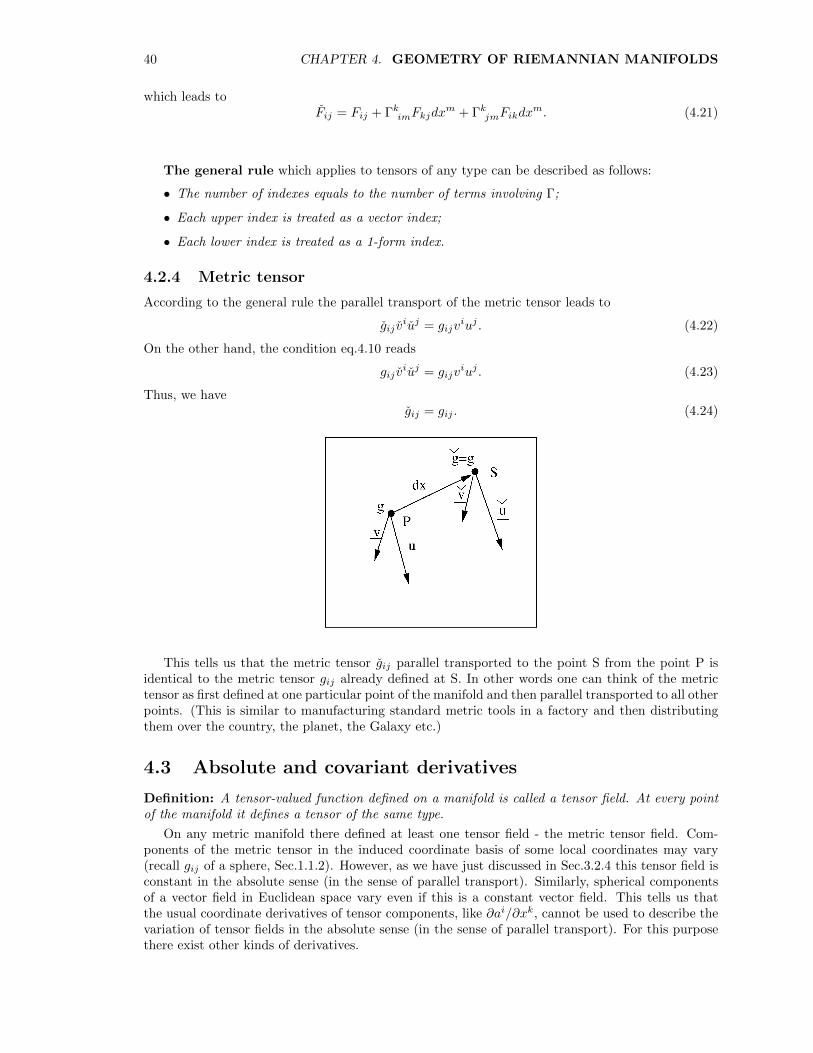
Thus, we havegij = gij . (4.24)
This tells us that the metric tensor gij parallel transported to the point S from the point P isidentical to the metric tensor gij already defined at S. In other words one can think of the metrictensor as first defined at one particular point of the manifold and then parallel transported to all otherpoints. (This is similar to manufacturing standard metric tools in a factory and then distributingthem over the country, the planet, the Galaxy etc.)
4.3 Absolute and covariant derivatives
Definition: A tensor-valued function defined on a manifold is called a tensor field. At every pointof the manifold it defines a tensor of the same type.
On any metric manifold there defined at least one tensor field - the metric tensor field. Com-ponents of the metric tensor in the induced coordinate basis of some local coordinates may vary(recall gij of a sphere, Sec.1.1.2). However, as we have just discussed in Sec.3.2.4 this tensor field isconstant in the absolute sense (in the sense of parallel transport). Similarly, spherical componentsof a vector field in Euclidean space vary even if this is a constant vector field. This tells us thatthe usual coordinate derivatives of tensor components, like ∂ai/∂xk, cannot be used to describe thevariation of tensor fields in the absolute sense (in the sense of parallel transport). For this purposethere exist other kinds of derivatives.
4.3. ABSOLUTE AND COVARIANT DERIVATIVES 41
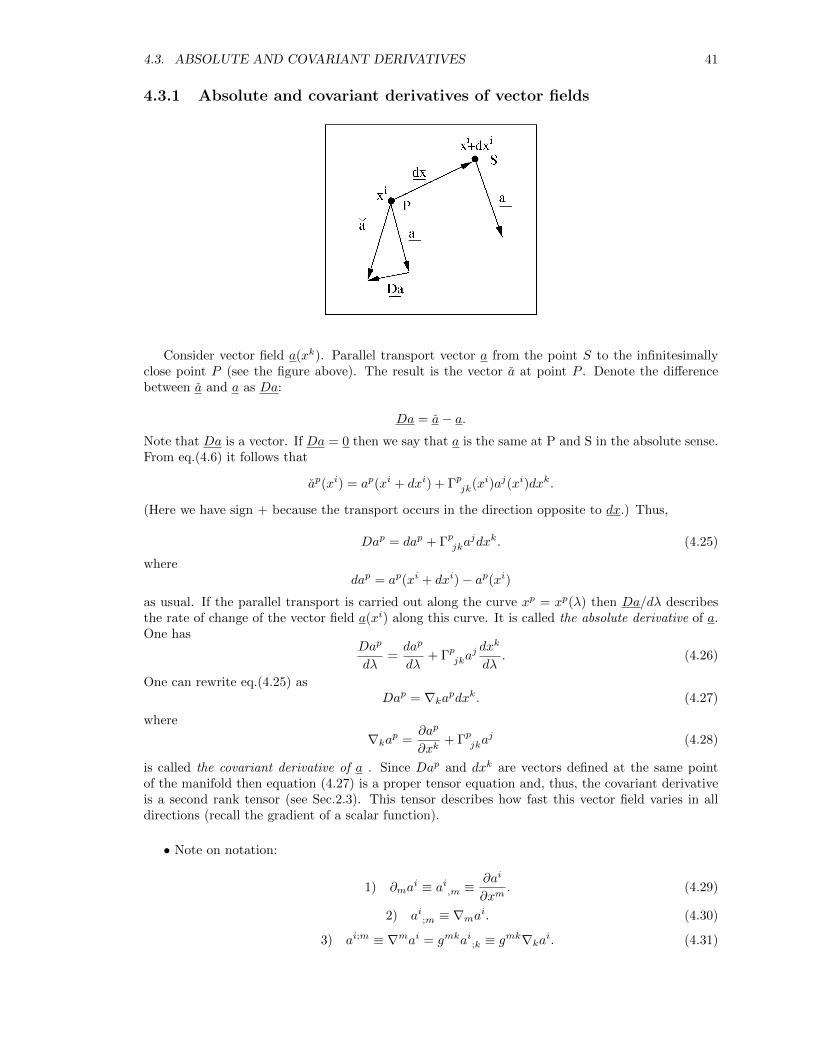
4.3.1 Absolute and covariant derivatives of vector fields
Consider vector field a(xk). Parallel transport vector a from the point S to the infinitesimallyclose point P (see the figure above). The result is the vector a at point P . Denote the differencebetween a and a as Da:
Da = a− a.Note that Da is a vector. If Da = 0 then we say that a is the same at P and S in the absolute sense.From eq.(4.6) it follows that
ap(xi) = ap(xi + dxi) + Γpjk(xi)aj(xi)dxk.
(Here we have sign + because the transport occurs in the direction opposite to dx.) Thus,
Dap = dap + Γpjkajdxk. (4.25)
wheredap = ap(xi + dxi)− ap(xi)
as usual. If the parallel transport is carried out along the curve xp = xp(λ) then Da/dλ describesthe rate of change of the vector field a(xi) along this curve. It is called the absolute derivative of a.One has
Dap
dλ=dap
dλ+ Γpjka
j dxk
dλ. (4.26)
One can rewrite eq.(4.25) asDap = ∇kapdxk. (4.27)
where
∇kap =∂ap
∂xk+ Γpjka
j (4.28)
is called the covariant derivative of a . Since Dap and dxk are vectors defined at the same pointof the manifold then equation (4.27) is a proper tensor equation and, thus, the covariant derivativeis a second rank tensor (see Sec.2.3). This tensor describes how fast this vector field varies in alldirections (recall the gradient of a scalar function).
• Note on notation:
1) ∂mai ≡ ai,m ≡
∂ai
∂xm. (4.29)
2) ai;m ≡ ∇mai. (4.30)
3) ai;m ≡ ∇mai = gmkai;k ≡ gmk∇kai. (4.31)
42 CHAPTER 4. GEOMETRY OF RIEMANNIAN MANIFOLDS
4.3.2 Absolute and covariant derivatives of 1-form fields
Similarly one obtains the following results for 1-forms
qp(xi) = qp(x
i + dxi)− Γjpk(xi)qj(xi)dxk.
Dqp = qp − qp = dqp − Γjpkqjdxk. (4.32)
wheredqp = qp(x
i + dxi)− qp(xi).
Note that Dq is a 1-form. The absolute derivative of q is
Dqpdλ
=dqpdλ− Γjpkqj
dxk
dλ. (4.33)
Dqp = ∇kqpdxk. (4.34)
where
∇kqp =∂qp∂xk− Γjpkqj (4.35)
is the covariant derivative of q . It is a second rank tensor which describes how fast the 1-form fieldvaries in all directions.
• Note on notation:
1) ∂mqi ≡ qi,m ≡∂qi∂xm
. (4.36)
2) qi;m ≡ ∇mqi. (4.37)
3) q ;mi ≡ ∇mqi = gmkqi;k ≡ gmk∇kqi. (4.38)
4.3.3 Absolute and covariant derivatives of general tensor fields
The same procedure applies to higher rank tensors. For example, for the field of second rank tensorT ij one obtains
DT ijdλ
= ∇mT ijdxm
dλ(4.39)
where
∇mT ij =∂T ij∂xm
+ ΓikmTkj − ΓkjmT
ik. (4.40)
General rule:
• The absolute derivative of a tensor field of rank r is a tensor or rank r;
• The covariant derivative of a tensor field of rank r is a tensor or rank r + 1;
• The first term in the expression for the covariant derivative is the usual partial coordinatederivative (∂/∂xm) of tensor’s components;
• There are r more terms in this expression, one per each index. In each such term for an upperindex this index is treated as a vector index and in each such term for a lower index it istreated as a 1-form index.
One more exampleDT ijsdλ
= ∇mT ijsdxm
dλ(4.41)
∇mT ijs =∂T ijs∂xm
+ ΓikmTkjs − ΓkjmT
iks − ΓksmT
ijk. (4.42)
4.4. GEODESICS AND PARALLEL TRANSPORT 43
4.3.4 Absolute and covariant derivatives of scalar fields
From eq.(4.15) it follows that for a scalar field f (scalar function)
Df
dλ= ∇mf
dxm
dλ(4.43)
∇mf =∂f
∂xm(4.44)
4.3.5 General properties of covariant differentiation
For any tensors A and B of the same type
∇m(A+B) = ∇mA+∇mB, (4.45)
and∇m(AB) = (∇mA)B +A(∇mB), (4.46)
where multiplication can be both inner and outer. Although the actual number and position ofindexes of A and B does not matter here (this is why their indexes are not shown) the general rulesof tensor equations still applies.
Examples:∇m(Aij +Bij) = ∇mAij +∇mBij ,
∇m(AiBi) = (∇mAi)Bi +Ai(∇mBi),
∇m(AiBj) = (∇mAi)Bj +Ai(∇mBj),
4.3.6 The field of metric tensor
Sincegij = gij
(see Sec.3.2.4) one hasDgijdλ
= 0 (4.47)
along any curve xi = xi(λ) and∇mgij = 0. (4.48)
4.4 Geodesics and parallel transport
We already know (see Sec.1.4) that geodesics are solutions of the Euler-Lagrange equations
d
dλ
∂L
∂xk− ∂L
∂xk= 0 (k = 1, 2, ..., n) (4.49)
with LagrangianL(xk, xk) = gij x
ixj . (4.50)
(Recall that xk = dxk/dλ where λ is a normal parameter of the geodesic.) It easy to see that
∂L
∂xk=∂gij∂xk
xixj and∂L
∂xk= 2gikx
i.
Substitution of these results into eq.(4.49) gives us
d
dλ(2gikx
i)− ∂gij∂xk
xixj = 0.

44 CHAPTER 4. GEOMETRY OF RIEMANNIAN MANIFOLDS
⇒ 2∂gik∂xj
xj xi + 2gikxi − ∂gij
∂xkxixj = 0.
⇒ gikxi +
1
2
(∂gik∂xj
+∂gjk∂xi
− ∂gij∂xk
)xixj = 0.
Now we can use eq.(4.12) and write this result as
gikxi + Γkij x
ixj = 0.
By raising index k (see eq.4.14 and eq.3.44) this is turned into the so-called geodesic equation
xk + Γkij xixj = 0 (4.51)
which is the same asDti
dλ= 0, (4.52)
where
ti =dxi
dλ(4.53)
is the tangent vector to the geodesic. In other words, the tangent vector ti is the same along thegeodesic in the absolute sense ( in the sense of parallel transport along the geodesic). This resultsallows to give the following alternative definition of a geodesic curve
Definition. A curve is called geodesic if it allows a parameter λ such that
Dti
dλ= 0, where ti =
dxi
dλ
Such parameter is called “normal” and ti is called ” the normal tangent vector”. It is this propertyof geodesics that is meant when they are described as the straightest possible curves.
4.5 Geodesic coordinates and Fermi coordinates
4.5.1 Geodesic coordinates
By definition, for any point of a Riemannian manifold one can find such a system of coordinates,called locally Cartesian that at this point
gij =
{1 if i = j0 if i 6= j
(4.54)
Moreover, for any point of a Riemannian manifold one can find such a system of coordinates that
Γijk = 0, (4.55)
and, hence,
gij,k = 0; (4.56)
∇m =∂
∂xm; (4.57)
D
dλ=
d
dλ. (4.58)
at this particular point. Such coordinates are call geodesic coordinates.Here is how geodesic coordinates coordinates can be set up. Select a point on the manifold where
the conditions (4.55-4.58) are to be satisfied. At this point, introduce a set of basis vectors, {ei},
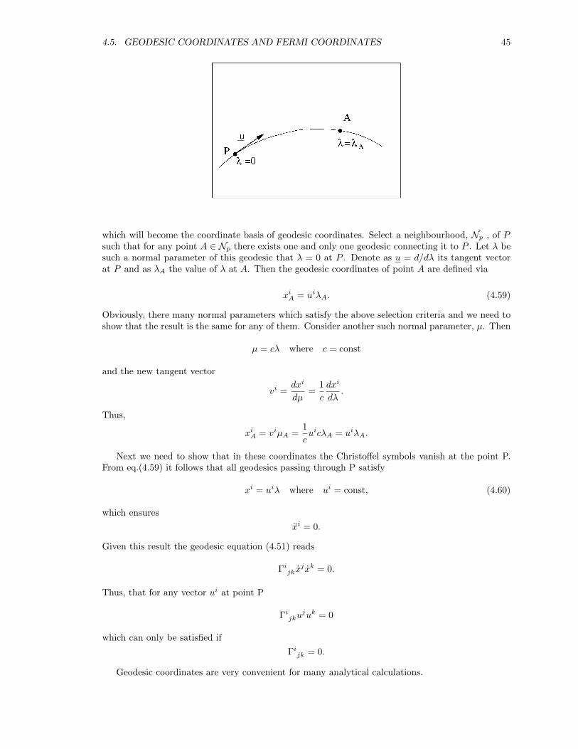
4.5. GEODESIC COORDINATES AND FERMI COORDINATES 45
which will become the coordinate basis of geodesic coordinates. Select a neighbourhood, Np , of Psuch that for any point A ∈ Np there exists one and only one geodesic connecting it to P . Let λ besuch a normal parameter of this geodesic that λ = 0 at P . Denote as u = d/dλ its tangent vectorat P and as λA the value of λ at A. Then the geodesic coordinates of point A are defined via
xiA = uiλA. (4.59)
Obviously, there many normal parameters which satisfy the above selection criteria and we need toshow that the result is the same for any of them. Consider another such normal parameter, µ. Then
µ = cλ where c = const
and the new tangent vector
vi =dxi
dµ=
1
c
dxi
dλ.
Thus,
xiA = viµA =1
cuicλA = uiλA.
Next we need to show that in these coordinates the Christoffel symbols vanish at the point P.From eq.(4.59) it follows that all geodesics passing through P satisfy
xi = uiλ where ui = const, (4.60)
which ensures
xi = 0.
Given this result the geodesic equation (4.51) reads
Γijkxj xk = 0.
Thus, that for any vector ui at point P
Γijkujuk = 0
which can only be satisfied if
Γijk = 0.
Geodesic coordinates are very convenient for many analytical calculations.
46 CHAPTER 4. GEOMETRY OF RIEMANNIAN MANIFOLDS
4.5.2 Fermi coordinates
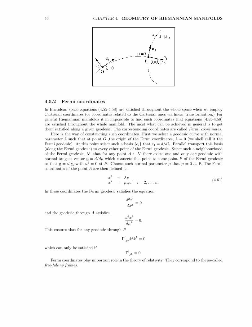
In Euclidean space equations (4.55-4.58) are satisfied throughout the whole space when we employCartesian coordinates (or coordinates related to the Cartesian ones via linear transformation.) Forgeneral Riemannian manifolds it in impossible to find such coordinates that equations (4.55-4.58)are satisfied throughout the whole manifold. The most what can be achieved in general is to getthem satisfied along a given geodesic. The corresponding coordinates are called Fermi coordinates.
Here is the way of constructing such coordinates. First we select a geodesic curve with normalparameter λ such that at point O ,the origin of the Fermi coordinates, λ = 0 (we shell call it theFermi geodesic). At this point select such a basis {ei} that e1 = d/dλ. Parallel transport this basis(along the Fermi geodesic) to every other point of the Fermi geodesic. Select such a neighbourhoodof the Fermi geodesic, N , that for any point A ∈ N there exists one and only one geodesic withnormal tangent vector u = d/dµ which connects this point to some point P of the Fermi geodesicso that u = uiei with u1 = 0 at P . Choose such normal parameter µ that µ = 0 at P. The Fermicoordinates of the point A are then defined as
x1 = λPxi = µAu
i i = 2, . . . , n.(4.61)
In these coordinates the Fermi geodesic satisfies the equation
d2xi
dλ2= 0
and the geodesic through A satisfiesd2xi
dµ2= 0.
This ensures that for any geodesic through P
Γijkxj xk = 0
which can only be satisfied ifΓijk = 0.
Fermi coordinates play important role in the theory of relativity. They correspond to the so-calledfree-falling frames.

4.6. RIEMANN CURVATURE TENSOR 47
4.6 Riemann curvature tensor
Parallel transport on Riemannian manifolds has a number of properties not seen in Euclidean space.This is clearly demonstrated in the following examples involving a 2D sphere. Recall that any vectortangent to a geodesic remains tangent during parallel transport along this geodesic. Moreover, sincethe angle between two parallel transported vectors is constant so must be the angle between a vectorparallel transported along a geodesic and this geodesic.
1. The result of parallel transport depends not only on the initial and final points but also on thepath along which this transport is carried out!
(a) When vector t is parallel transported from the point A on the equator to the north pole,N , along the meridian AN the result is vector t′;
(b) When vector t is first parallel transported from the point A to the point C along theequator, which results in vector t∗, and then parallel transported from C to N along themeridian CN the result is a different vector, t′′ 6= t′.
2. Parallel transport along a closed curve does not result in the original vector!
Indeed, when vector t′ is parallel transported along the closed path NACN the result is vectort′′
Obviously these peculiar properties stem from the fact that sphere is a curved surface! Curvatureof such surfaces and general manifolds is described via the so called Riemann curvature tensor.
48 CHAPTER 4. GEOMETRY OF RIEMANNIAN MANIFOLDS
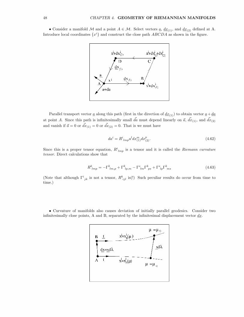
• Consider a manifold M and a point A ∈ M. Select vectors a, dx(1), and dx(2) defined at A.
Introduce local coordinates {xi} and construct the close path ABCDA as shown in the figure.
Parallel transport vector a along this path (first in the direction of dx(1)) to obtain vector a+da
at point A. Since this path is infinitesimally small ~da must depend linearly on ~a, ~dx(1), and ~dx(2)
and vanish if ~a = 0 or ~dx(1) = 0 or ~dx(2) = 0. That is we must have
dai = Rilmpaldxm(1)dx
p(2). (4.62)
Since this is a proper tensor equation, Rilmp is a tensor and it is called the Riemann curvaturetensor. Direct calculations show that
Rklmp = −Γklm,p + Γklp,m − ΓslmΓkps + ΓslpΓkms (4.63)
(Note that although Γijk is not a tensor, Rkijl is(!) Such peculiar results do occur from time totime.)
• Curvature of manifolds also causes deviation of initially parallel geodesics. Consider twoinfinitesimally close points, A and B, separated by the infinitesimal displacement vector dx.
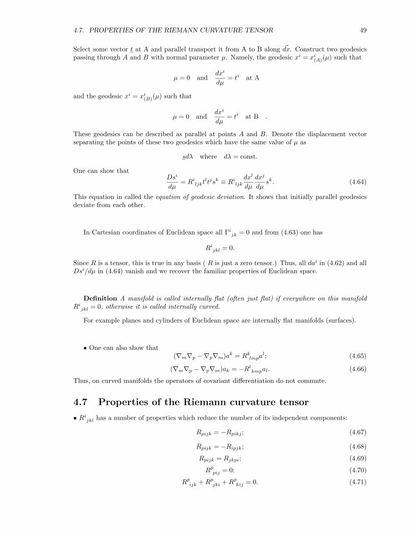
4.7. PROPERTIES OF THE RIEMANN CURVATURE TENSOR 49
Select some vector t at A and parallel transport it from A to B along ~dx. Construct two geodesicspassing through A and B with normal parameter µ. Namely, the geodesic xi = xi(A)(µ) such that
µ = 0 anddxi
dµ= ti at A
and the geodesic xi = xi(B)(µ) such that
µ = 0 anddxi
dµ= ti at B .
These geodesics can be described as parallel at points A and B. Denote the displacement vectorseparating the points of these two geodesics which have the same value of µ as
sdλ where dλ = const.
One can show thatDsi
dµ= Riljkt
ltjsk ≡ Riljkdxl
dµ
dxj
dµsk. (4.64)
This equation in called the equation of geodesic deviation. It shows that initially parallel geodesicsdeviate from each other.
In Cartesian coordinates of Euclidean space all Γijk = 0 and from (4.63) one has
Rijkl = 0.
Since R is a tensor, this is true in any basis ( R is just a zero tensor.) Thus, all dai in (4.62) and allDsi/dµ in (4.64) vanish and we recover the familiar properties of Euclidean space.
Definition A manifold is called internally flat (often just flat) if everywhere on this manifoldRijkl = 0, otherwise it is called internally curved.
For example planes and cylinders of Euclidean space are internally flat manifolds (surfaces).
• One can also show that(∇m∇p −∇p∇m)ak = Rklmpa
l; (4.65)
(∇m∇p −∇p∇m)ak = −Rlkmpal. (4.66)
Thus, on curved manifolds the operators of covariant differentiation do not commute.
4.7 Properties of the Riemann curvature tensor
• Rijkl has a number of properties which reduce the number of its independent components:
Rpijk = −Rpikj ; (4.67)
Rpijk = −Ripjk; (4.68)
Rpijk = Rjkpi; (4.69)
Rppij = 0; (4.70)
Rpijk +Rpjki +Rpkij = 0. (4.71)
50 CHAPTER 4. GEOMETRY OF RIEMANNIAN MANIFOLDS
Note the cyclic permutation of the lower indexes in eq.(4.71). The best way of proving theseproperties involves use of geodesic coordinates. Indeed, since in geodesic coordinates Γijk = 0and gij,k = 0, eq.(4.63) has a much simpler form
Rklmp = −Γklm,p + Γklp,m . (4.72)
Using eq.(4.12) this can also be written as
Rklmp =1
2[gkp,lm + glm,kp − gkm,lp − glp,km] (4.73)
(By the way, eq.(4.73) tells us that all second order derivatives of gij vanish only if Rijkl = 0!) Nowit easy to see that, for example,
Rklmp = −Γklm,p + Γklp,m = −(Γklm,p − Γklp,m) = −(−Γklp,m + Γklm,p) = Rklpm,
which proves eq.(4.67).Because of the properties (4.67-4.71) the curvature tensor has only
N =1
12n2(n2 − 1)
independent components (the total number of components is n4, where n is the dimension of themanifold.) If n = 2 then N = 1. The curvature tensor of 2D manifolds has only one independentcomponent.• One can also show (using geodesic coordinates once again) that
Rikpl;m +Riklm;p +Rikmp;l = 0 (4.74)
(Note the cyclic permutation of indexes p, l,m in this equation.) This result is known as the Bianchiidentity.
4.8 Ricci tensor, curvature scalar and the Einstein tensor
These important tensors are derived from the Riemann curvature tensor. The Ricci tensor is definedvia
Rij = Rsisj (4.75)
The symmetries (4.67-4.69) ensue that
Rij = −R si sj = −Rsijs = R s
si j , (4.76)
as well asRij = Rji. (4.77)
The curvature scalar is defined asR = Rii. (4.78)
The Einstein tensor is
Gij = Rij −1
2Rgij . (4.79)
It is easy to seeGij = Gji. (4.80)
Moreover, using the Bianchi identity one can show that
Gik;k ≡ ∇kGsk ≡ 0. (4.81)
In other words, the divergence of Einstein’s tensor is zero.
Chapter 5
Space and time in the theory ofrelativity
Each physical theory is based on a number of key assumptions - the rest of the theory is then buildon these assumptions using appropriate mathematical tools. Any good theory has to be
1. self-consistent (no internal contradictions),
2. consistent with Nature.
It seems like the second condition can never be achieved completely. As we learn more we discovernew, previously unknown contradictions between our theories and Nature. They force us to reviseour theories by constructing new sets of basic assumptions.
What was revised during the transition from from Newtonian physics to General Relativity arethe assumptions on the nature of physical time and space.
5.1 Physical Space and Time in Newtonian Physics
• Time: Physical time is absolute – it is the same everywhere in the Universe. Thus, it can bemeasured by a single standard clock and can be modeled as a one-dimensional metric spacewith coordinate t. This t is a convenient universal parameter for trajectories of particles.
• Space: Physical space is also absolute - it is the same at any time. For any moment of timeone can introduce Cartesian coordinates covering the whole physical space. Thus, this is aEuclidean space.
• Inertial frames: In order to describe motion/evolution of physical systems we need to havea system of spatial coordinates at any time. This can be arranged by building a spatial grid- a system of physical objects (nodes) which may or may not be kept at the same distancefrom each other. Such spatial grid is called a reference frame. Depending of the problemunder consideration some of these references frames are better than others as they provide asimple description of the studied phenomena. In particular, the motion of free particles hasa particularly simple form when described in so-called inertial frames where they move withconstant speed:
Dvi
dt= 0, (5.1)
51

52 CHAPTER 5. SPACE AND TIME IN THE THEORY OF RELATIVITY
where
vi =dxi
dtor v =
d
dt.
One can think of an inertial frame as a collection of free particles moving with the same speed,so that the distances between them are fixed, the grid of spatial coordinates being attached tothese particle. These spatial coordinates do not have to be Cartesian – the use of the absolutederivative in eq.5.1 ensures that the choice of spatial coordinates is not important. Sinceeq.5.1 in nothing else but the geodesic equation, the trajectory of free particle is a geodesic ofEuclidean space. The absolute time t is a normal parameter of this geodesic, and vi = dxi/dtis its tangent vector.
In Cartesian coordinates eq.5.1 can be written as
dvi
dt= 0, or
d2xi
dt2= 0.
If the particle is subject to a force f the law of motion becomes
D(mvi)
dt= f i. (5.2)
where scalar m is the particle’s mass.
• Newtonian principle of relativity:
There are infinitely many inertial frames and there is no way to tell which of them are movingand which of them are at rest in space. All laws of mechanics are exactly the same for all ofthem. Thus, there is no absolute motion, that is a motion relative to the space itself, but onlythe relative motion, that is a motion of some objects relative to others.
5.2 Physical Space and Time in Special Relativity
• Time, Space and Inertial Frames. Various experiments show that in vacuum electromag-netic waves propagate with the same speed, c, relative to all inertial observers. Moreover,c is the maximum possible speed for any signal. This implies that time can no longer beconsidered as absolute because there is no unambiguous way of determining simultaneity ofspatially separated events. (Only if there existed a way of communicating information withinfinitely large speed then simultaneity would have an absolute meaning.) This also explainswhy moving relative to each other inertial observers measure different time intervals betweenthe same events even if they use identical clocks and identical procedures. Because, time isno longer absolute, an inertial frame of Special Relativity is no longer just a collection of freeparticles moving with the same velocity and carrying the spacial grid. They should also carrysynchronized clocks used to measure time of this particular frame.
Physical space is not absolute either as different inertial observers obtain different resultswhen they measure lengths of the same objects even if they use identical standard meters andidentical procedures. This implies that physical space can not be described as a metric space.
However, all inertial observers obtain the same result for the spacetime interval
∆s2 = −c2∆t2 + ∆l2 (5.3)
for any two events. This suggests to unite physical time and space into a single 4-dimensionalmetric space, called spacetime, and consider ∆s as a generalised distance between its points,called events. If ∆s2 > 0 then there exists a frame where ∆t = 0 and ∆s2 = ∆l2. Suchspacetime intervals are called space-like. If ∆s2 < 0 then there exists a frame where ∆l = 0and ∆s2 = −c2∆t2. Such spacetime intervals are called time-like. Spacetime intervals such

5.2. PHYSICAL SPACE AND TIME IN SPECIAL RELATIVITY 53
that ∆s2 = 0 are called null. They cannot be reduced to either pure space or pure timeintervals. (If fact they describe events on the world-line of a light signal.)
Here are the basic assumptions on the nature of spacetime in Special Relativity:
1. Spacetime is a 4-dimensional metric space. If {xν}, ν = 0, 1, 2, 3, are arbitrary coordinatesof the spacetime then the interval between its infinitesimally close points is given by themetric form
ds2 = gµνdxµdxν where µ, ν = 0, 1, 2, 3. (5.4)
2. There exist such coordinate systems that
(a) The hyper-surfaces x0 =const have purely space-like metric form
dl2 = gijdxidxj i, j = 1, 2, 3, (5.5)
with gij independent on x0;
(b) The spacetime metric (5.4) reduces to
ds2 = −(dx0)2 + dl2. (5.6)
Such coordinate systems correspond to inertial frames with spatial coordinates xi,i = 1, 2, 3, and global time
t = x0/c.
(c) There exist such spatial coordinates xi that that
dl2 = (dx1)2 + (dx2)2 + (dx3)2
throughout the whole hypesurface x0 =const. Thus, this hypersurface is a 3-dimensionalEuclidean space.
In other words, spacetime allows coordinates {xν} such that
ds2 = −(dx0)2 + (dx1)2 + (dx2)2 + (dx3)2 (5.7)
and, hence,
gµν =
−1 0 0 0
0 1 0 00 0 1 00 0 0 1
(5.8)
throughout the whole spacetime. These coordinates are called pseudo-Cartesian. Metricspaces which allow such coordinates are called pseudo-Euclidean (or Minkowskian).
• Einstein’s principle of relativity:
Einstein assumed that not only mechanical laws but all physical laws are exactly the same inall inertial frames. Thus, the idea of absolute motion is completely rejected. This is known asEinstein’s principle of relativity. Introduction of spacetime allows us to transform this principleinto a simple prescription for writing relativistic laws of physics. Indeed, as we have alreadyseen, different inertial frames correspond to different systems of coordinates in spacetime. Thusif we write laws of physics in the form which does not involve coordinates whatsoever thenthey will automatically satisfy the principle of relativity. Tensor equations involving spacetimetensors fit into this category perfectly well.
For example, consider the motion of free particles. In spacetime each particle traces a curvewhich is called its world-line. One can use the particle’s proper time, τ , as a parameter of thecurve. The tangent vector
~u =d
dτor uν =
dxν
dτ(5.9)
54 CHAPTER 5. SPACE AND TIME IN THE THEORY OF RELATIVITY
is called the 4-velocity of the particle. Note that this is a spacetime vector. Now consider thefollowing tensor equation
Duν
dτ= 0. (5.10)
In the pseudo-Cartesian coordinates of any inertial frame this reads
duν
dτ= 0 or uν = const. (5.11)
Thus,
cdt
dτ= const and
dxi
dτ= const,
which gives usdxi
dt= const or
dvi
dt= 0. (5.12)
Since in Cartesian coordinatesdvi
dt=Dvi
dt
we have recovered the 3-tensor equation (5.12) of motion of free particles:
Dvi
dt= 0.
Thus, (i) the 4-tensor eq.(5.10) is the law of motion of free particles; (ii) from this 4-tensorequation there follows the 3-tensor law of motion which has the same invariant form for allinertial frames (in agreement with the principle of relativity).
5.3 Relativistic equations of motion of particle dynamics
The 4-tensor equation of motion of free particles (eq.5.10),
Duν
dτ= 0,
is nothing else but the geodesic equation. Thus, world lines of free particles are geodesics ofspacetime. Since uνu
ν < 0 they are time-like geodesics. Using the spacetime connection thisequation can be written as
duν
dτ+ Γνµηu
µuη = 0. (5.13)
and, finally, as a system of second order PDEs for xν(τ)
d2xν
dτ2+ Γνµη
dxµ
dτ
dxη
dτ= 0. (5.14)
(This is the most general form of equations of motions of free particles which holds for anysystem of spacetime coordinates.)
In pseudo-Cartesian coordinates all Christoffel’s symbols vanish and eq.(5.14) reduces to
d2xν
dτ2= 0, (5.15)
which immediately integrates to give
xν = aντ + bν where aν , bν = const.
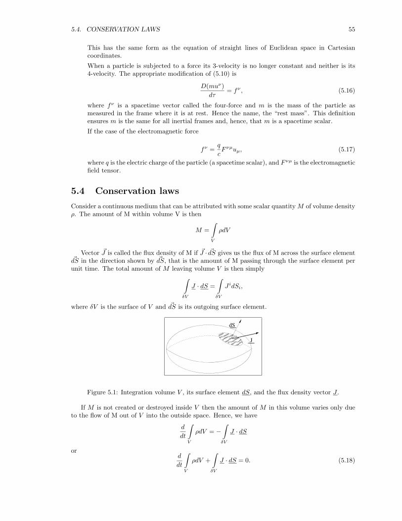
5.4. CONSERVATION LAWS 55
This has the same form as the equation of straight lines of Euclidean space in Cartesiancoordinates.
When a particle is subjected to a force its 3-velocity is no longer constant and neither is its4-velocity. The appropriate modification of (5.10) is
D(muν)
dτ= fν , (5.16)
where fν is a spacetime vector called the four-force and m is the mass of the particle asmeasured in the frame where it is at rest. Hence the name, the “rest mass”. This definitionensures m is the same for all inertial frames and, hence, that m is a spacetime scalar.
If the case of the electromagnetic force
fν =q
cF νµuµ, (5.17)
where q is the electric charge of the particle (a spacetime scalar), and F νµ is the electromagneticfield tensor.
5.4 Conservation laws
Consider a continuous medium that can be attributed with some scalar quantity M of volume densityρ. The amount of M within volume V is then
M =
∫V
ρdV
Vector ~J is called the flux density of M if ~J · ~dS gives us the flux of M across the surface element~dS in the direction shown by ~dS, that is the amount of M passing through the surface element perunit time. The total amount of M leaving volume V is then simply∫
δV
J · dS =
∫δV
J idSi,
where δV is the surface of V and ~dS is its outgoing surface element.
���������������������������������������������������������������������������������������������������������������������������������������������������������
���������������������������������������������������������������������������������������������������������������������������������������������������������
J
dS
Figure 5.1: Integration volume V , its surface element dS, and the flux density vector J .
If M is not created or destroyed inside V then the amount of M in this volume varies only dueto the flow of M out of V into the outside space. Hence, we have
d
dt
∫V
ρdV = −∫δV
J · dS
ord
dt
∫V
ρdV +
∫δV
J · dS = 0. (5.18)
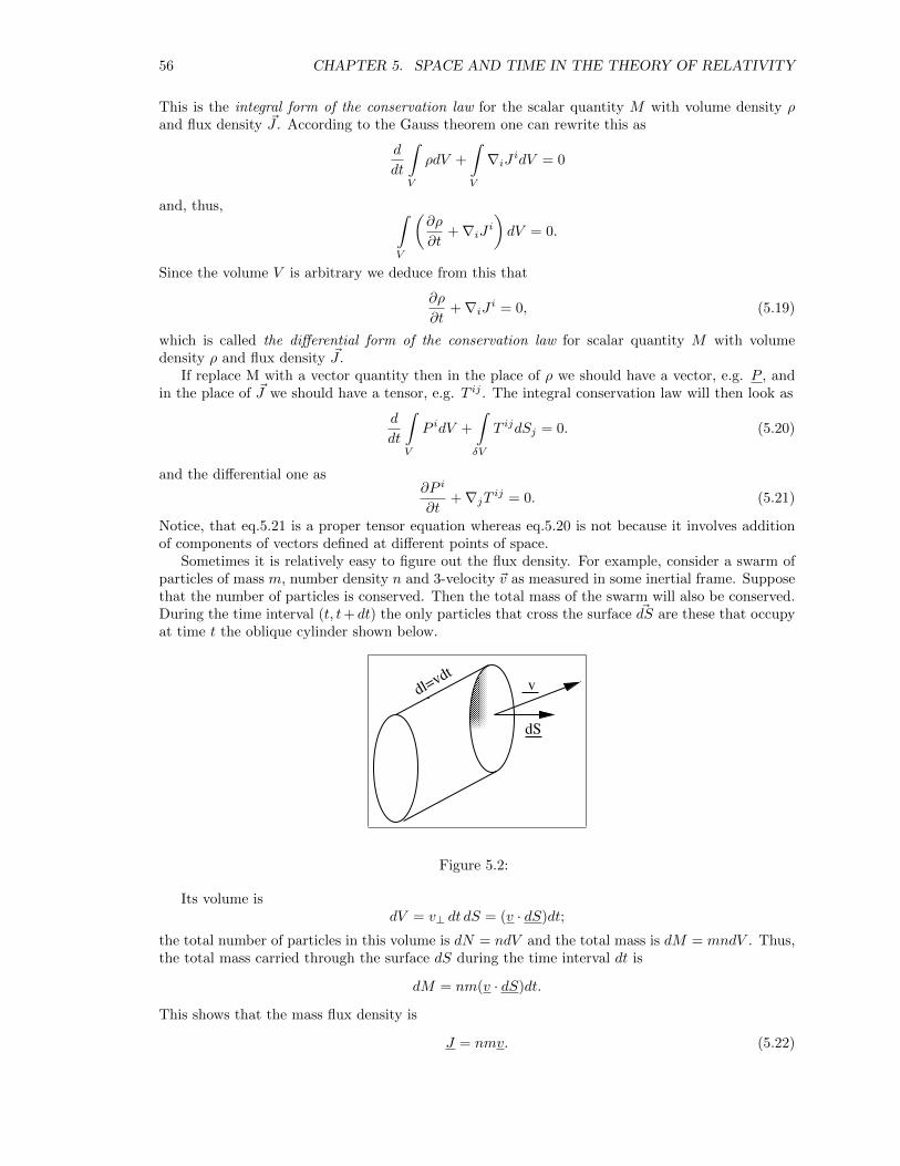
56 CHAPTER 5. SPACE AND TIME IN THE THEORY OF RELATIVITY
This is the integral form of the conservation law for the scalar quantity M with volume density ρand flux density ~J . According to the Gauss theorem one can rewrite this as
d
dt
∫V
ρdV +
∫V
∇iJ idV = 0
and, thus, ∫V
(∂ρ
∂t+∇iJ i
)dV = 0.
Since the volume V is arbitrary we deduce from this that
∂ρ
∂t+∇iJ i = 0, (5.19)
which is called the differential form of the conservation law for scalar quantity M with volumedensity ρ and flux density ~J .
If replace M with a vector quantity then in the place of ρ we should have a vector, e.g. P , andin the place of ~J we should have a tensor, e.g. T ij . The integral conservation law will then look as
d
dt
∫V
P idV +
∫δV
T ijdSj = 0. (5.20)
and the differential one as∂P i
∂t+∇jT ij = 0. (5.21)
Notice, that eq.5.21 is a proper tensor equation whereas eq.5.20 is not because it involves additionof components of vectors defined at different points of space.
Sometimes it is relatively easy to figure out the flux density. For example, consider a swarm ofparticles of mass m, number density n and 3-velocity ~v as measured in some inertial frame. Supposethat the number of particles is conserved. Then the total mass of the swarm will also be conserved.During the time interval (t, t+ dt) the only particles that cross the surface ~dS are these that occupyat time t the oblique cylinder shown below.
���������������������������������������������������������������������������������������������������������������������
���������������������������������������������������������������������������������������������������������������������
vdl=vdt
dS
Figure 5.2:
Its volume isdV = v⊥ dt dS = (v · dS)dt;
the total number of particles in this volume is dN = ndV and the total mass is dM = mndV . Thus,the total mass carried through the surface dS during the time interval dt is
dM = nm(v · dS)dt.
This shows that the mass flux density is
J = nmv. (5.22)
5.5. RELATIVISTIC CONTINUITY EQUATION 57
5.5 Relativistic continuity equation
Consider a swarm of particles moving with four-velocity uν . Let n be the number density of theseparticles as measured in the inertial frame moving with the same velocity as the local velocity of theswarm. It is called the proper number density. Consider the following 4-tensor equation
∇ν(nuν) = 0. (5.23)
Here ∇ν is the operator of covariant differentiation in spacetime. Notice that n is a spacetime scalar,∇µ(nuν) is a spacetime tensor, and hence ∇ν(nuν) is a spacetime scalar. Thus, equation (5.23) isa proper tensor equation and may express a physical law (see the principle of relativity). But whatlaw? In the pseudo-Cartesian coordinates of an arbitrary inertial frame, laboratory frame,
∇ν =∂
∂xνand uν = γ(c, v1, v2, v3) (5.24)
where γ is the Lorentz factor and vi is the usual velocity vector (three-vector). Thus, (5.23) reads
∂
∂x0(γcn) +
∂
∂xi(γnvi) = 0 (5.25)
Since x0 = ct and in Cartesian coordinates
∇i =∂
∂xi
this can also be written as
∂
∂t(γn) +∇i(γnvi) = 0 (5.26)
or
∂
∂t(n) +∇i(nvi) = 0 (5.27)
where n = γn is the number density of particles as measured in the laboratory frame, it is differentfrom n because of the Lorentz contraction. (Notice that∇i is the operator of covariant differentiationin space, the hypersurface x0 =const.) Obviously, eq.(5.26) describes the conservation of particles asseen in the laboratory frame and, thus, the 4-tensor equation (5.23) describes the same conservationbut in a coordinate independent form.
Introduce the proper rest mass density of the swarm,
ρ = mn. (5.28)
Since the rest mass m is a spacetime scalar we can now rewrite (5.23) as
∇ν(ρuν) = 0. (5.29)
This 4-tensor equation is called the relativistic continuity equation.
5.6 Stress-energy-momentum tensor
5.6.1 Energy-momentum vector
Consider a particle of rest mass m and 4-velocity uν . The 4-vector
P ν = muν (5.30)
is called the energy-momentum vector of the particle (or its4-momentum vector). In the laboratoryframe
P ν = mγ(c, v1, v2, v3) = (E/c, p1, p2, p3), (5.31)
58 CHAPTER 5. SPACE AND TIME IN THE THEORY OF RELATIVITY
whereE = mγc2 (5.32)
is the particle energy andpi = mγvi (5.33)
is the 3-vector of particle’s momentum as measured in the laboratory frame.
m = mγ (5.34)
is called the inertial mass of the particle, it’s mass as measured in the laboratory frame. Fromeq.(5.12) it follows that for a free particle
E = const and pi = const. (5.35)
Thus, the energy and the momentum of a free particle are conserved. The 4-tensor equation withdescribes this conservation is
DPµ
dτ= 0. (5.36)
5.6.2 Stress-energy-momentum tensor of dust
Consider now a swarm of free particles of the proper number density n, the proper rest mass densityρ = mn, and the 4-velocity uν . The tensor
Tµν = ρuµuν (5.37)
is called the stress-energy-momentum tensor of the swarm. Components of this tensor also allowsimple interpretation. Consider an arbitrary inertial frame (the laboratory frame). Denote as e theenergy density (per unit volume), as πi the momentum density and as si the energy flux density ofthe swam in this frame. Then
e = T 00, πi = (1/c)T 0i = (1/c)T i0, si = cT 0i = cT i0. (5.38)
Moreover, T ij if the momentum flux density, the stress 3-tensor. (T ij gives us the flux density ofthe i-component of momentum in the j-direction, and, at the same time, the flux density of thej-component of momentum in the i-direction.) Indeed,
•e = ρu0u0 = ργ2c2 = (mγc2)(nγ) = En; (5.39)
•πi = ρu0ui/c = ργ2vi = (mγvi)(nγ) = pin; (5.40)
•si = cρu0ui = ργ2c2vi = evi; (5.41)
•T ij = ρuiuj = (ργ2vi)vj = πivj ; (5.42)
andT ij = ρuiuj = (ργ2vj)vi = πjvi. (5.43)
Thus, like the usual energy and momentum of a single particle are simply components of a firstrank 4-tensor ( energy-momentum vector), the usual energy density, momentum density, energy fluxdensity and stress tensor (3-tensor) of a continuously distributed system are components of a secondrank 4-tensor (stress-energy-momentum tensor).
5.6. STRESS-ENERGY-MOMENTUM TENSOR 59
5.6.3 Energy-momentum conservation
Consider the following equation
∇νTµν = 0. (5.44)
Since this is a 4-tensor equation it may express some physical law. But what law? In the pseudo-Cartesian coordinates of the laboratory frame
∇µ =∂
∂xµ. (5.45)
Thus, eq.(5.44) reads∂
∂xνTµν = 0 (5.46)
or∂
∂x0Tµ0 +
∂
∂xiTµi = 0 (5.47)
or1
c
∂
∂tTµ0 +
∂
∂xiTµi = 0. (5.48)
The time component of this equation (µ = 0) can be written as
∂
∂te+∇isi = 0. (5.49)
This is just the energy conservation law. The spatial component (µ = 1, 2, 3) of eq.(5.48) reads as
∂
∂tπj +∇iT ji = 0. (5.50)
This is just the momentum conservation law. Thus eq.(5.44) describes the conservation of energyand momentum in a coordinate independent form.
5.6.4 Stress-energy-momentum tensor of perfect fluid
Any continuous system like a fluid or a force field can be attributed with its own stress-energy-momentum tensor and if this system is isolated (does not interact with other systems) then eq.(5.44)is satisfied.
Let us determine the stress-energy-momentum tensor of ideal fluid. What we need is an expres-sion for this 4-tensor in terms of lower rank (more basic) 4-tensors like in eq.(5.37). But it is easierto figure out the components of T ij in the rest frame of the fluid. (By this we mean the inertialframe where the fluid is at rest. Obviously, each fluid element has it own rest frame.) In the restframe the energy per unit volume is given by
T 00 = e = ρc2 + ε,
their ρ is the rest mass density and ε is the thermal energy density. Moreover, since vi = 0 themomentum density and hence the energy flux density vanish in this frame
πi = T 0i = T i0 = 0.
The components of stress tensor of ideal fluid at rest in Cartesian coordinates are
T ij =
p 0 00 p 00 0 p
where p is the thermodynamic pressure. Thus, in the pseudo-Cartesian coordinates of the rest framethe components of stress-energy momentum tensor of ideal fluid are

60 CHAPTER 5. SPACE AND TIME IN THE THEORY OF RELATIVITY
Tµν =
e 0 0 00 p 0 00 0 p 00 0 0 p
. (5.51)
Note that e and p are spacetime scalars. They completely determine the thermodynamical stateof ideal fluid. Its motion is completely determined by the 4-vector uν . Thus, what we need to donow is to construct T νµ from e, p, and uν via suitable tensor operations in such a way that in thefluid frame we end up with eq.(5.51). In fact,
Tµν = (e+ p
c2)uµuν + pgµν (5.52)
does the job. Indeed, in the pseudo-Cartesian coordinates of the rest frame of the fluid
uν = (c, 0, 0, 0)
gµν =
−1 0 0 0
0 1 0 00 0 1 00 0 0 1
,
and eq.(5.52) reduces to eq.(5.51).

5.7. SPACE AND TIME IN GENERAL RELATIVITY 61
5.7 Space and Time in General Relativity
The key idea of General Relativity is that gravitational interaction makes itself felt via producinginternal curvature of spacetime. The following example from Newtonian mechanics helps to under-stand this idea. Consider the motion of particles bound to a spherical surface but otherwise free ofany force. Such particle simply move along geodesics of the sphere (with constant speed). Thesegeodesics are great circles. Consider two such particles initially located on the equator with paralleland equal initial velocities. As they move in the direction of the north pole they accelerate towardeach other as if they were under the action of a mutual attraction force.
• Space and Time: The spacetime is no longer a flat pseudo-Euclidean space but a curvedpseudo-Riemannian manifold. This manifold is only locally pseudo-Euclidean which meansthat one can introduce local coordinates such that
gµν =
−1 0 0 0
0 1 0 00 0 1 00 0 0 1
, (5.53)
at a single point but not throughout the manifold. All basic results from the theory of Rie-mannian manifolds apply to pseudo-Riemannian manifolds.
• Inertial frames: There are no global inertial frames in General Relativity. Indeed, the cur-vature of spacetime (inflicted by gravitational interactions) does not allow us to introduceglobal pseudo-Cartesian coordinates. However, one can introduce local pseudo-Cartesian co-ordinates, like geodesic coordinates or Fermi coordinates. These correspond to locally inertialframes. In particularly, the Fermi coordinates built around a time-like geodesic correspondto a small free-falling laboratory. Within the small volume of such a laboratory the effects offinite curvature of spacetime are also very small.
• General Principle of Relativity: It is not possible to detect the effects of gravitationalinteraction via local measurements. In other words, via experiments carried out within asufficiently small free-falling laboratory, one can not detect the presence of nearby gravitatingbodies. For example, the astronauts on board of a space station orbiting the Earth and theastronauts on board of a spacecraft free flying far away from Earth, in almost empty deepspace, share exactly the same experiences, e.g. weightlessness. This implies that, all localphysical laws (laws formulated in terms of quantities defined at a single point of spacetime)must have exactly the same form as in the flat spacetime of Special Relativity and, hence, theRiemann curvature tensor can not appear in them. (The only exception are the equations
62 CHAPTER 5. SPACE AND TIME IN THE THEORY OF RELATIVITY
of gravitational field which show how exactly the curvature is imposed on spacetime.) Forexample, the motion of free particles is still described by equation (5.1),
Duµ
dτ= 0,
and, thus, their world lines are still geodesics of spacetime. Similarly, the motion of ideal fluid(and dust) is still described equations (5.29,5.44),
∇νρuν = 0,
∇µT νµ = 0.
5.8 Einstein’s equations of gravitational field
Let us speculate on how the equations of gravitational field could look like. Obviously they must betensor equations and should involve the Riemann curvature tensor. If this curvature is caused bymatter then some tensor fields describing the distribution of matter must also be involved.
In Newtonian gravity matter is present in the form of its volume mass density. But in relativisticphysics things are different in two respects:
1. Mass is attributed not only to matter but also to force fields (like the electromagnetic field)via m = E/c2. This suggests that not only matter but also force field can curve spacetime.
2. The volume mass density (or energy density) is not a spacetime scalar but just one componentof the stress-energy-momentum tensor. This suggests to seek a simple tensor equation relatingthe Riemann curvature tensor with T νµ, the total stress-energy-momentum tensor!
The metric tensor may also be present in this equation because of it fundamental role in geometry.However, the equation must agree with the symmetries of involved tensors. It does not seem possibleto relate T νµ and gµν with Rνµηπ directly. For example, the equation
Rνµηπ = agµνTηπ
is in conflict with the symmetries of the Riemann curvature tensor (eqs.4.67-4.71). However, theRicci tensor has the same rank and the same symmetry as T νµ and initially Einstein suggested that
Rνµ = aT νµ,
where a is a constant. However, he quickly realised that this is no good. Indeed, because
∇µRνµ 6= 0
one ends up with∇µT νµ 6= 0
which contradicts to the general principle of relativity. So, Einstein suggested another equationwhich is free from such a flaw, namely
Gνµ = aT νµ, (5.54)
where Gνµ = Rνµ− (R/2)gνµ is now known as the Einstein tensor. Indeed, as we have already seen(equation 4.81),
∇µGνµ ≡ 0
implying∇µT νµ = 0. (5.55)
Equation (5.54) is known as the Einstein equation of gravitational field. Later we shell see that
a =8πG
c4(5.56)

5.8. EINSTEIN’S EQUATIONS OF GRAVITATIONAL FIELD 63
The Einstein equation (5.54) is the key equation of General Relativity. Once this equation isintroduced we can forget all the reasons which have led Einstein to this equation and simply derivefrom it all the important results of the Theory of Relativity. For example, as we have already seen,equation (5.55) follows directly from the Einstein equation. This equation describes the dynamicsof continuous media like fluids and fields. For a swarm of dust particles
Tµν = ρuµuν , (5.57)
where ρ = mn is the rest mass density of the swarm (see Sec.4.5.2). Hence, eq.(5.55) reads
∇νTµν = ∇νρuνuµ = ρuν∇νuµ + uµ∇νρuν = 0. (5.58)
Since these particle do not interact with each other their total number is conserved and we have
∇νρuν = 0. (5.59)
This allows us to write eq.(5.58) as
ρuν∇νuµ = 0,
orDuν
dτ= 0.
This is the equation of motion of free particles (geodesic motion).Now we may consider a time-like geodesic of a free falling laboratory and construct the corre-
sponding system of Fermi coordinates of this geodesic. Since in these coordinates
Γνµη = 0D
dt=
d
dtand ∇ν =
∂
∂xν
along the geodesic (notice that here τ = t) the equations of continuous dynamics, (5.55) and (5.59)reduce to
∂
∂xµT νµ = 0,
and∂
∂xµρuµ = 0,
and the equation of geodesic motion reduces to
duν
dt= 0.
This is exactly how they read in the pseudo-Cartesian coordinates of flat spacetime. Thus, gravity“disappears” in free falling locally inertial frames.
Einstein’s equation can be written in slightly different form which we shell use later on. Toobtain this, we first contract (eq.5.54)
Gνν = aT νν or Rνν −1
2Rδνν = aT νν
Next we denote
T νν as T (5.60)
and use that δνν = 4 to obtain
R = −aT. (5.61)
Finally, substitute this into (5.54) to obtain
Rνµ = a(T νµ − 1
2Tgνµ). (5.62)
64 CHAPTER 5. SPACE AND TIME IN THE THEORY OF RELATIVITY
We know that components of the Riemann curvature tensor in the coordinate basis are functionsof Γνµη and Γνµη,β . We also know that Γνµη are functions of gνµ and gνµ,β . Thus, the components ofRµνηγ , and hence the components of Rνµ and Gνµ, depend on the components of gνµ and their firstand second partial derivatives. Thus, the Einstein equations can be viewed as second order partialdifferential equations for the components of the metric tensor! The total number of independentequations in this system is 10 ( Do you know why?) The same is the total number of independentcomponents of the metric tensor. What a match! However, rather complicated analysis of theEinstein equations shows that they include only 6 evolution equations that describe the “time-evolution” of gµν . Others may be consider as differential constrains on the initial solution (like
∇ ~B = 0 in electrodynamics). Thus, there in no match after all and the system appears to be under-determined. In fact, this is good news! Indeed, the components of metric tensor depend not only onthe structure of the spacetime but also on the system of coordinates we choose. When we introducefour coordinates in spacetime we effectively impose four additional conditions on the components ofmetric tensor. And in reverse, an introduction of four additional conditions on the components ofmetric tensor amounts to setting up a coordinate system. Here is two examples of such conditions:
• The conditionsg00 = −1, gi0 = 0.
define the so-called “time-orthogonal coordinates” (they may not exist).
• The conditionsgµνΓβµν = 0, which ensure ∇µ∇µxβ = 0,
introduce the so-called “harmonic coordinates”.
Often one cannot give a clear physical interpretation of coordinates introduced in such a way (e.g.one cannot tell which coordinate is time-like and which are space-like). Only after the Einsteinequations are solved and the functions gνµ(xβ) are found such an interpretation becomes possible.
In fact, the Einstein equations are local and do not tell anything about the spacetime topology.We have to make explicit assumptions on the topology of spacetime – for example, we may assumethat it has the same topology as a 4-dimensional sphere of a 5-dimensional Euclidean space. Butwill this be a correct assumption?

5.9. NEWTONIAN LIMIT 65
5.9 Newtonian limit
The Newtonian theory of gravity has been extremely successful. It describes the motion of planetsand satellites with great accuracy. This means that in the limit of low velocities and hence weakgravity any good theory of gravity must reduce to the Newtonian theory. Let us check that theEinstein theory satisfies this condition.
Here is the basic equations of the Newtonian theory.
• The equation of motion (the second law of particle mechanics):
~a = −~∇Φ orDvi
dt= −∇iΦ, (5.63)
where ~v is the particle velocity, ~a is the particle acceleration, and Φ is the gravitational poten-tial.
• The equation of gravitational field:∆Φ = 4πGρ, (5.64)
where ρ is the mass density, G is the gravitational constant, and
∆ = ∇i∇i = gij∇i∇j
is the Laplace operator.
In Cartesian coordinates {xi} these equations read
dvi
dt= − ∂Φ
∂xi(5.65)
and3∑i=1
∂2Φ
∂xi2 = 4πGρ. (5.66)
The basic equations of the Einstein theory are
• The equation of motion:Duν
dτ= 0, (5.67)
• The field equation:
Rµν = a(Tµν −1
2Tgµν). (5.68)
What are the conditions of weak gravity?
1. The curvature of spacetime must be very small. Thus, there must be possible to constructsuch a system of coordinates that the metric tensor has almost the same components as in flatspacetime (Minkowskian) in pseudo-Cartesian coordinates. That is
gµν = ηµν + hµν , (5.69)
where
ηµν =
−1 0 0 0
0 1 0 00 0 1 00 0 0 1
, (5.70)
and|hµν | � 1. (5.71)

66 CHAPTER 5. SPACE AND TIME IN THE THEORY OF RELATIVITY
2. Moreover, the particle velocity must be much lower than the speed of light. Hence, we mayassume
u0 = c, and |ui| � c. (5.72)
This ensures that the proper time of the particle, τ , is very close to the coordinate timet = x0/c:
τ = t. (5.73)
Moreover, given such low characteristic speeds
∂
∂x0≈(vc
) ∂
∂xi� ∂
∂xi. (5.74)
3. Finally, for a nonrelativistic thermal motion (low temperatures)
ρc2 � ε, p. (5.75)
This means that only the rest mass of gravitating objects makes any noticeable contributionto their stress-energy-momentum tensors. Thus, the gravitational field is fully determined bythe distribution of rest mass.
Conditions (5.72) and (5.75) show that the T00 component of the Tµν tensor is much larger thanall other components and we may assume that
Tµν =
ρc2 0 0 00 0 0 00 0 0 00 0 0 0
(5.76)
with great accuracy.Let us check if under these conditions the Einstein equations (5.67) and (5.68) reduce to the
Newtonian equations (5.65) and (5.66). Let us start with the equation of motion. Using (5.73) onecan write the spatial part of (5.67) as
dui
dt+ Γiµνu
µuν = 0.
Using (5.72) this can be written asdui
dt+ Γi00c
2 = 0. (5.77)
From (4.12) we have
Γαµν =1
2gαγ
[∂gγµ∂xν
+∂gγν∂xµ
− ∂gµν∂xγ
].
Substituting gνµ from (5.69-5.71) and keeping only the terms first order in h we obtain
Γαµν =1
2ηαγ
[∂hγµ∂xν
+∂hγν∂xµ
− ∂hµν∂xγ
], (5.78)
which gives us
Γi00 =1
2ηiγ[∂hγ0∂x0
+∂hγ0∂x0
− ∂h00∂xγ
].
Since ηνµ is diagonal we have
Γi00 =1
2ηii[∂hi0∂x0
+∂hi0∂x0
− ∂h00∂xi
]=
1
2
[∂hi0∂x0
+∂hi0∂x0
− ∂h00∂xi
].
Finally, using (5.74) we may ignore the derivative with respect to x0 and obtain
5.9. NEWTONIAN LIMIT 67
Γi00 = −1
2
∂h00∂xi
. (5.79)
Then eq.(5.77) reads
dui
dt=c2
2
∂h00∂xi
. (5.80)
Notice that this equation has exactly the same form as (5.65). This suggests to relate h00 withNewtonian gravitational potential via
Φ = −c2
2h00. (5.81)
Let us now deal with the field equation. From eq.(5.76) we find
T00 = ρc2 and T = T νν = T 00 = η00T00 = −ρc2.
Thus, the time component of (5.68) reads
R00 =a
2ρc2. (5.82)
Equation (5.78) shows that all components of Γ are small (of order O(h)). Keeping only termslinear in Γ we can write
Rαβγδ =∂
∂xγΓαβδ −
∂
∂xδΓαβγ
(see eq.4.63) and thus
R00 = Rα0α0 =∂
∂xαΓα00 −
∂
∂x0Γα0α.
Once again we may ignore derivatives with respect to x0 and obtain
R00 =∂
∂xiΓi00.
Substitution of Γi00 from (5.79) into this equation gives us
R00 = −1
2
3∑i=1
∂2h00
∂xi2 .
Thus, equation (5.82) reads
−1
2
3∑i=1
∂2h00
∂xi2 =
a
2ρc2. (5.83)
Using eq.(5.81) we can write this as3∑i=1
∂2Φ
∂xi2 =
ac4
2ρ. (5.84)
This equation has exactly the same form as the Newtonian field equation (5.66). Thus, Einstein’sequations do reduce to the Newtonian equations indeed! Moreover, now we can express constant aof the Einstein equations in terms the gravitational constant, G, and the speed of light:
a =8πG
c4. (5.85)
68 CHAPTER 5. SPACE AND TIME IN THE THEORY OF RELATIVITY

Chapter 6
Schwarzschild Solution
In this chapter we study a particular solution of Einstein’s equations that describes the spacetimeoutside of a spherically symmetric non-rotating body of a certain mass, e.g. a non-rotating blackhole, and the motion of test particles in such spacetime. Throughout this chapter we use therelativistic units, also known as the geometric units, where G = 1 and c = 1.
6.1 Schwarzschild Solution
6.1.1 Schwarzschild Solution in Schwarzschild coordinates
The interval of pseudo-Euclidean spacetime of special relativity in pseudo-Cartesian coordinates isgiven by
ds2 = −dt2 + dx2 + dy2 + dz2
For problems with spherical symmetry in space (t =const hypersurface) it is more convenient to usespherical spatial coordinates {r, θ, φ}. Then the spacetime interval takes the following form:
ds2 = −dt2 + dr2 + r2(dθ2 + sin2 θdφ2).
Now, let us try to come up with a simple and reasonable expression for the metric form of thespacetime about a stationary spherically symmetric body of total mass m. When we say “stationary”we mean that it must be possible to introduce such a reference frame that the spatial location ofthe body remains fixed forever. In such frame the components of metric tensor cannot depend ontime t. (Far away from the body this t must tick at the same rate as the proper time of observersat rest relative to mass m. )
If the body is spherically symmetric then we expect the spacetime to be spherically symmetric aswell. Therefore, like in Euclidean space, we should be able to introduce spatial coordinates {r, θ, φ}such that the line element depends on the angles θ and φ only via the combination
dθ2 + sin2 θdφ2.
Thus, we expect the metric form to have the following structure
ds2 = −a(r,m)dt2 + b(r,m)dr2 + c(r,m)r2(dθ2 + sin2 θdφ2). (6.1)
There three unknown functions, they are a(r,m), b(r,m), and c(r,m), in this expression1. It can bereduced to two, if we redefine r via
(r′)2 = c(r,m)r2.
1Notice that we introduced more than 4 additional constraints on the components of metric tensor assuming themetric form (6.1) (see the discussion at the end of Sec.5.8)
69

70 CHAPTER 6. SCHWARZSCHILD SOLUTION
Then, (6.1) reads
ds2 = −A(r,m)dt2 +B(r,m)dr2 + r2(dθ2 + sin2 θdφ2) (6.2)
where we have omitted ′, or
gµν =
−A(r,m) 0 0 00 B(r,m) 0 00 0 r2 00 0 0 r2 sin2 θ
.
Far away from this body we expect the curvature gradually reduce to zero. In other words, weexpect the spacetime to become flat at spatial infinity, that is
A,B → 1 as r →∞. (6.3)
In fact we can impose even more restrictive constraint on A(r,m). Indeed, given the results ofSec.5.9, we may assume that far away from the body
A = 1− htt = 1 + 2Φ = 1− 2m/r. (6.4)
(Here htt is the same as h00 in Sec.5.9)This is how we think the metric tensor should look like in some suitable coordinates {t, r, θ, φ}.
It remains to be seen that Einstein’s equations do indeed allow solutions of this form. The requiredcomputations are carried out as follows: (i) compute gµν,γ , (ii) then gµν,γδ, (iii) then Rµνγδ, (iv)then Rµν , (v) then Gµν . To find the solution describing spacetime outside of the body we need tosubstitute the result into the vacuum version of Einstein’s equations:
Gνµ = 0.
This gives us a system of second order ordinary differential equations for A(r,m) and B(r,m) (notethat m is a parameter, not a variable.) which we need to solve subject to conditions at infinity. Thegeneral solution of those equation is
A(r,m) = a(m)− b(m)/r,
B(r,m) = c(m)/A(r,m).
Conditions (6.3,6.4) are satisfied by A(r,m) if
a(m) = 1, b(m) = 2m,
and the condition (6.3) is satisfied ifc(m) = 1.
Thus, the final result is
ds2 = −(1− 2m/r)dt2 + (1− 2m/r)−1dr2 + r2(dθ2 + sin2 θdφ2) (6.5)
orgµν = 0 if ν 6= µ
gtt = −(1− 2m/r), grr = (1− 2m/r)−1, gθθ = r2, gφφ = r2 sin2 θ.
This solution is known as the Schwarzschild solution and the coordinates {t, r, θ, φ} are called theSchwarzschild coordinates. If the radius of the body is r∗ then it holds only for r > r∗. However, theSchwarzschild solution also describes the spacetime of a black hole – in such case it applies for r > 0.To be more precise, this solution applies only to non-rotating objects. Rotation inflicts additionalcurvature on spacetime.
6.1. SCHWARZSCHILD SOLUTION 71
Let us analyse the nature of the Schwarzschild coordinates.
• For any r > 0
gθθ =~∂
∂θ·~∂
∂θ> 0, gφφ =
~∂
∂φ·~∂
∂φ> 0
and, thus, θ and φ are space-like coordinates.
• For r > 2m
gtt =~∂
∂t·~∂
∂t< 0, grr =
~∂
∂r·~∂
∂r> 0
and, thus, t is a time-like coordinate and r is a space-like one as expected.
• However, for r < 2m
gtt =~∂
∂t·~∂
∂t> 0, grr =
~∂
∂r·~∂
∂r< 0
and, thus, r is a time-like coordinate and t is a space-like one. Hence the lesson: Do notassume that the coordinate denoted as t always refers to time measurements! Be prepared tounexpected!
One can see that r = 0 is special. gtt and grr → ∞ as r → 0. In fact, the curvature scalar Ralso tends to ∞. At this point the curvature of spacetime becomes infinite. This is a real spacetimesingularity of the Schwarzschild solution – the place where the approximation of General Relativitybreaks down.
6.1.2 Schwarzschild Solution in Kerr coordinates
r = 2m is also rather special as grr → ∞ as r → 2m. However, R remains finite and hence thecurvature of spacetime is finite. There is no spacetime singularity on this surface. In fact, onthis surface the system of Schwarzschild coordinates becomes singular. It is possible to introduceother coordinate systems that are free from such singularity. One example is the system of Kerrcoordinates which is introduced as follows:
• r, θ, and φ are the same as in Schwarzschild coordinates,
• New t′ = t′(t, r) coordinate is introduced via the following transformation, singular at r = 2m:
dt′ = dt− (1− r/2m)−1dr, (6.6)
or∂t′
∂t= 1
∂t′
∂r= (1− r/2m)−1
Notice that Maxwell’s integrability condition
∂2t′
∂t∂r=
∂2t′
∂r∂t
is satisfied by the transformation (6.6)
Substitution of dt from (6.6) into (6.5) gives
ds2 = −(1− 2m/r)dt′2 + (4m/r)dt′dr + (1 + 2m/r)dr2 + r2(dθ2 + sin2 θdφ2). (6.7)
One can see that now all components of the metric tensor are finite at r = 2m and, thus, there isno singularity there. Moreover, now the r-coordinate is always space-like. Notice, that eqs.(6.5) and(6.7) describe the same spacetime (In what follows we will no longer use ′ to indicate Kerr’s time.)

72 CHAPTER 6. SCHWARZSCHILD SOLUTION
6.1.3 Event horizon
Is it always possible to have a physical object, say a test particle, at rest relative to a black hole,that is with fixed r, θ, φ coordinates? The spacetime interval along the world-line of any particle isnegative
ds2 = −dτ2,where τ is the proper time of the particle. For a stationary particle
dr = dθ = dφ = 0
and, thus, along its world-line one has
ds2 = −(1− 2m/r)dt2
which is negative if r > 2m and positive if r < 2m. Thus, no stationary particle, as well as nostationary physical observer, can exist at r < 2m!
If inside r = 2m particles must be moving then what kind of motion is it? It is easy to see thatall terms on the right side in eq.(6.7) are non-negative if r < 2m except the second one, which mayboth positive and negative. Hence, if ds2 is negative then so must be this second term. This means
drdt < 0 and, hence, dr/dt < 0.
Thus the particle is forced to move inwards, toward the physical singularity at r = 0. The criticalradius rg = 2m is called the gravitational or Schwarzschild radius (in generic units rg = 2Gm/c2)and the surface r = rg is called the event horizon as nothing can escape from inside of this surfaceinto the outside space. Whatever event occurs inside the event horizon the outside observers are notreceiving any information about it.
ExerciseDetermine the distance Lhs between the horizon and the singularity along the radial direction of
Kerr coordinates (t, θ, φ = const).
Solution: In Kerr coordinates
~∂
∂r·~∂
∂r= grr = 1 + 2m/r > 0
and, thus, along the radial direction
ds2 = dl2 = grrdr2 > 0.
This is a space-like direction. Hence,
Lhs =
r=2m∫r=0
dl =
2m∫0
√grrdr =
2m∫0
√1 + 2m/rdr
If we introduce new variable y =√r/2m then
Lhs = 4m
1∫0
√1 + y2dy.
Given that ∫ √1 + y2dy =
1
2
[y√
1 + y2 + ln(y +√
1 + y2)]
we finally obtain
Lhs = 2m[√
2 + ln(1 +√
2)].
6.2. GRAVITATIONAL REDSHIFT 73
6.2 Gravitational redshift
Consider the Schwarzschild solution in Schwarzschild coordinates:
ds2 = −(1− 2m/r)dt2 + (1− 2m/r)−1dr2 + r2(dθ2 + sin2 θdφ2). (6.8)
Consider an observer at rest (dr = dθ = dφ = 0) at infinity. If τ∞ is the proper time of this observerthen
dτ2∞ = −ds2 = dt2. (6.9)
Thus, the coordinate t that selects the spacetime hypersurface t = const may be interpreted as thetime measured by an observer at rest at infinity by means of a standard clock.
Consider another observer at rest at 2m < r <∞. His/her proper time is
dτ2r = −ds2 = (1− 2m/r)dt2 (6.10)
and, thus,
dτ2r = (1− 2m/r)dτ2∞ (6.11)
Notice, that dτr < dτ∞. This property is often described as slowing down of clocks ( or evenof time) in gravitational field. In fact, this is exactly what a distant observer watching a standardclock of another observer, placed near a gravitating body, will see.
Consider two observers, A and B, resting at r = ra and r = rb respectively (both outside thehorizon). The interval of coordinate time δt required for a light signal emitted by A to reach Bdoes not depend on the time of emission because the components of metric tensor in Schwarzschildcoordinates do not depend on t. To illustrate this point consider the case where both observersare situated along the same radial direction (θa = θb, φa = φb. This simplifies the calculations.)Due to the spherical symmetry of spacetime the light signal has to propagate along the same radialdirection and the spacetime interval along its world-line is given by
ds2 = gttdt2 + grrdr
2 = 0.
Therefore,
dt2 = (−grr/gtt)dr2
and
δt =
∣∣∣∣∣∣rb∫ra
√(−grr/gtt)dr
∣∣∣∣∣∣ . (6.12)
Since gµν do not depend on t so does not δt.Suppose A emits two signals separated by the interval ∆t of the coordinate time t. When B
receives these signals they are still separated by the same interval ∆t. Indeed, if they are emittedat t = 0 and ∆t then they are received at t = δt and ∆t + δt. For the same reason, if A emits aperiodic signal of period ∆t of coordinate time t, B records the same period. However, the propertime τ measured by standard clocks of the observers run at rates different from the rate of t. Fromeq.6.10 one has
∆τ2a = (1− 2m/ra)∆t2, ∆τ2b = (1− 2m/rb)∆t2
and, thus,
∆τ2a =
(1− 2m/ra1− 2m/rb
)∆τ2b . (6.13)
If rb =∞ then we have

74 CHAPTER 6. SCHWARZSCHILD SOLUTION
∆τ2a = (1− 2m/ra)∆τ2∞. (6.14)
Thus, if A emits a periodic signal with the period of its standard clock then B at r = ∞ will seethat this clock runs slower than his/her own standard clock. Notice, that eq.6.14 has exactly thesame form as eq.6.11.
On the other hand, ∆τ could be just a period of a monochromatic electromagnetic wave emittedby A as measured by his/her standard clock. Since the frequency of the wave ν = 1/∆τ , we have
ν2a =
(1− 2m/rb1− 2m/ra
)ν2b . (6.15)
If rb > ra then νb < νa. Thus, the frequency of an electromagnetic wave is decreasing as the wavepropagates away from the source of gravity. This effect is called the gravitational redshift. (Opticallines shift toward the red part of the spectrum).
6.3 Integrals of motion of free test particles in Schwarzschildspacetime
By test particles we understand particles of such a small mass that their gravitational field is neg-ligibly small compared to the field of other involved objects. Such particles can be used to test thegravitational field created by those bodies without disturbing them. Hence the name test particles.In Sec.5.3,5.7 we have learned that the equation of motion of a free particle is
Duα
dτ= 0, (6.16)
and, hence, its world-line is a geodesic of spacetime.From Sec.4.4 ( just substitute λ with τ) we know that the geodesic equations can be can be
written as the Euler-Lagrange equations
d
dτ
∂L∂uµ
− ∂L∂xµ
= 0 (6.17)
with the Lagrangian
L(xν , uµ) = gαβ(xν)uαuβ . (6.18)
These equations allows us to derive a number of very important results on the motion of test particlesin the Schwarzschild spacetime in a rather easy way.
• Both in the Schwarzschild and Kerr coordinates
∂gαβ∂t
= 0
and, thus,
∂L∂t
= 0. (6.19)
From (6.17) and (6.19) one hasd
dτ
∂L∂ut
= 0,
and, thus, dL/dut is an integral of motion, which means that it is constants along the world-lineof the particle. In fact,
∂L∂ut
=∂(gνµu
νuµ)
∂ut= 2gtνu
ν = 2ut.
6.3. INTEGRALS OFMOTIONOF FREE TEST PARTICLES IN SCHWARZSCHILD SPACETIME75
Thus, we conclude that
ut = E = const. (6.20)
At infinity, where both in Schwarzschild and Kerr coordinates the metric attains its Minkowskianform, one has
E = ut = gtνuν = gttu
t = −ut = −γ = −Epmp
(6.21)
where Ep is the energy of the particle as measured by an observer at rest and mp is the restmass of the particle. For this reason −E is called the specific energy at infinity.
• Moreover, both in the Schwarzschild and Kerr coordinates
∂gαβ∂φ
= 0
and, thus,
∂L∂φ
= 0 andd
dτ
∂L∂uφ
= 0. (6.22)
Since
∂L∂uφ
=∂(gνµu
νuµ)
∂uφ= 2gφνu
ν = 2uφ,
we conclude that
uφ = l = const (6.23)
is another integral of motion. It is called the specific angular momentum at infinity.
• Since gµν depend on r and θ we conclude that ur and uθ are not integrals of motion!
• However, a test particle with initial uθ = 0 placed in the equatorial plane, θ = π/2 remains inthis plane forever. Since the direction of the polar axis is not restricted (spherical symmetry!)this result simply tells us that the motion of free particles in Schwarzschild geometry is planar.
Let us derive this results. Consider the θ-component of (6.17):
d
dτ
∂L∂uθ− ∂L∂θ
= 0. (6.24)
∂L∂θ
=∂(gνµu
νuµ)
∂θ=∂gφφ∂θ
uφuφ =
=∂(r2 sin2 θ)
∂θuφuφ = 2 cos θ sin θr2(uφ)2.
uφ = gφφuφ =1
gφφl =
l
r2 sin2 θ
Thus,∂L∂θ
=2 cos θl2
r2 sin3 θ. (∗)
Next,∂L∂uθ
=∂(gνµu
νuµ)
∂uθ= 2gθνu
ν = 2gθθuθ = 2r2uθ. (∗∗)
76 CHAPTER 6. SCHWARZSCHILD SOLUTION
Substitution of (*) and (**) into (6.24) gives
d
dτ
(r2dθ
dτ
)− cos θl2
r2 sin3 θ= 0. (6.25)
It is easy to see that θ(τ) = π/2 satisfies this equation. Moreover, this is the unique solutionsatisfying the initial conditions {
θ(τ0) = π/2dθ/dτ(τ0) = 0
(The theorem of uniqueness for second order ODEs.)
ExerciseA meteorite falls radially from rest at infinity into a Schwarzschild black hole. Show that in
Schwarzschild coordinatesur = −
√2m/r.
SolutionAt infinity
ui = 0, γ = 1 and, thus, E = −1.
Since the fall is radial, uθ = uφ = 0, the condition
gµνuµuν = −1
readsgttu
tut + grrurur = −1. (+)
Using E one can eliminate ut from this equation. Indeed,
ut = gttut =1
gttE = − 1
gtt
Thus, eq.(+) reads
gtt1
g2tt+ grru
rur = −1.
Now we can find ur = ur(r):
(ur)2 = −(1 + 1/gtt)/grr = −(1− 1
1− 2m/r)(1− 2m/r) =
= −((1− 2m/r)− 1) = 2m/r.

6.4. ORBITS OF TEST PARTICLES IN THE SCHWARZSCHILD GEOMETRY 77
6.4 Orbits of test particles in the Schwarzschild geometry
Consider the Schwarzschild solution in the Schwarzschild coordinates:
ds2 = −(1− rg/r)dt2 + (1− rg/r)−1dr2 + r2(dθ2 + sin2 θdφ2).
We already know that motion of test particles in the Schwarzschild spacetime is planar. We canalways choose the coordinates in such a way that the plane of motion becomes the equatorial plane,θ = π/2. Then uθ = 0 and the condition
gµνuµuν = −1
reads
gttutut + grru
rur + gφφuφuφ = −1. (6.26)
Sinceut = gttut = E/gtt and uφ = gφφuφ = l/gφφ,
eq.(6.26) readsE2
gtt+
l2
gφφ+ grru
rur = −1.
or
E2 + (1 +l2
gφφ)gtt + grrgtt(u
r)2 = 0. (∗)
For θ = π/2 one has
gφφ = r2, grr = (1− rg/r)−1, gtt = −(1− rg/r),
and eq.(*) reduces to(ur)2 + (1− rg/r)(1 + l2/r2) = E2.
Thus, we obtain(ur)2 + Φl(r) = E2, (6.27)
where
Φl(r) = (1− rg/r)(1 + l2/r2) (6.28)
From (6.27) one finds
dur
dτ= −1
2
dΦldr
(6.29)
This explains why Φ is called the effective potential.In the important case of a circular orbit
ur = 0, anddur
dτ= 0,
and equations (6.27) and (6.29) reduce to
Φl(r) = E2, (6.30)
and
dΦldr
= 0 (6.31)
respectively. These equations can be used to find the constants of motion, E and l, of circular orbits.Before we proceed with the analysis of let us briefly review the Newtonian results.
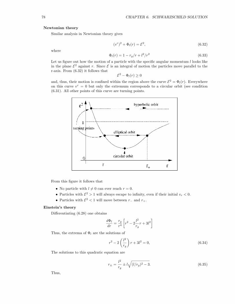
78 CHAPTER 6. SCHWARZSCHILD SOLUTION
Newtonian theory
Similar analysis in Newtonian theory gives
(vr)2 + Φl(r) = E2, (6.32)
whereΦl(r) = 1− rg/r + l2/r2 (6.33)
Let us figure out how the motion of a particle with the specific angular momentum l looks likein the plane E2 against r. Since E is an integral of motion the particles move parallel to ther-axis. From (6.32) it follows that
E2 − Φl(r) ≥ 0
and, thus, their motion is confined within the region above the curve E2 = Φl(r). Everywhereon this curve vr = 0 but only the extremum corresponds to a circular orbit (see condition(6.31). All other points of this curve are turning points.
From this figure it follows that
• No particle with l 6= 0 can ever reach r = 0.
• Particles with E2 > 1 will always escape to infinity, even if their initial vr < 0.
• Particles with E2 < 1 will move between r− and r+.
Einstein’s theory
Differentiating (6.28) one obtains
dΦldr
=rgr4
[r2 − 2
l2
rgr + 3l2
]Thus, the extrema of Φl are the solutions of
r2 − 2
(l2
rg
)r + 3l2 = 0, (6.34)
The solutions to this quadratic equation are
r± =l2
rg± l√
(l/rg)2 − 3. (6.35)
Thus,
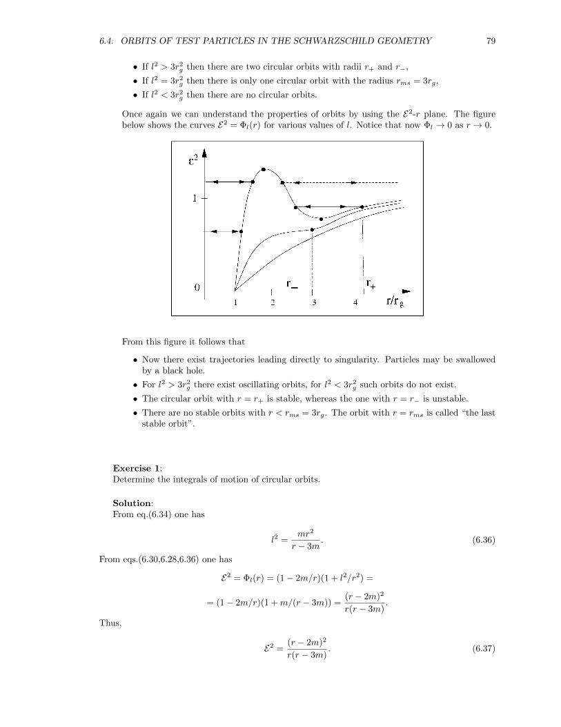
6.4. ORBITS OF TEST PARTICLES IN THE SCHWARZSCHILD GEOMETRY 79
• If l2 > 3r2g then there are two circular orbits with radii r+ and r−,
• If l2 = 3r2g then there is only one circular orbit with the radius rms = 3rg,
• If l2 < 3r2g then there are no circular orbits.
Once again we can understand the properties of orbits by using the E2-r plane. The figurebelow shows the curves E2 = Φl(r) for various values of l. Notice that now Φl → 0 as r → 0.
From this figure it follows that
• Now there exist trajectories leading directly to singularity. Particles may be swallowedby a black hole.
• For l2 > 3r2g there exist oscillating orbits, for l2 < 3r2g such orbits do not exist.
• The circular orbit with r = r+ is stable, whereas the one with r = r− is unstable.
• There are no stable orbits with r < rms = 3rg. The orbit with r = rms is called “the laststable orbit”.
Exercise 1:Determine the integrals of motion of circular orbits.
Solution:From eq.(6.34) one has
l2 =mr2
r − 3m. (6.36)
From eqs.(6.30,6.28,6.36) one has
E2 = Φl(r) = (1− 2m/r)(1 + l2/r2) =
= (1− 2m/r)(1 +m/(r − 3m)) =(r − 2m)2
r(r − 3m).
Thus,
E2 =(r − 2m)2
r(r − 3m). (6.37)
80 CHAPTER 6. SCHWARZSCHILD SOLUTION
Exercise 2:A spaceship is orbiting a black hole of mass m. Given that its orbit is circular one with radius r
determine the orbital period as measured by(i) a passenger of the spaceship, T(i),(ii) a stationary observer far away from the hole (at infinity), T(ii).
Solution:(i) The period T(i) is measured by a standard clock carried with the ship. Its time is the proper
time of the ship, τ . Since
uφ =dφ
dτ
one hasT(i) = 2π/uφ.
But
uφ = gφφuφ = l/gφφ =1
r2
(mr2
r − 3m
)1/2
=
=1
r
(m
r − 3m
)1/2
.
Hence,
T(i) = 2πr
(r − 3m
m
)1/2
.
(ii) The period T(ii) is measured by a standard clock at rest at infinity. It runs with the samerate as t (see Sec.6.2). Hence,
T(ii) =dt
dτT(i) = utT(i).
But
ut = gttut = E/gtt = − 1
1− 2m/r
(− r − 2m√
r(r − 3m)
)=
√r
r − 3m.
Thus,
T(ii) =
√r
r − 3m2πr
√r − 3m
m= 2πr
√r/m.
6.5 Perihelion shift of planets
The biggest success of Newtonian theory of gravity is the great accuracy with which it describes themotion of planets around Sun. For example, it predicts that the planetary orbits are not exactlyelliptical. The closest point of a planetary orbit, called perihelion, gradually moves (precesses) inthe orbital plane due to the gravitational interaction with other planets. This is indeed what isobserved. However, by the beginning of last century a small annoying disagreement between thetheory and measurements of the precession of the closest planet to Sun, Mercury, was becomingapparent. General relativity explains this result.
Let us find the equation for the trajectory of test particle in Schwarzschild geometry. SelectSchwarzschild coordinates in such a way that the orbital plane has θ = π/2. From eq.6.27 we have
(ur)2 = E2 − (1− rg/r)(1 + l2/r2).
Next,
uφ = gφφuφ =l
gφφ=
l
r2.

6.5. PERIHELION SHIFT OF PLANETS 81
Combining these two results we find(dr
dφ
)2
=
(ur
uφ
)2
=E2 − (1− rg/r)(1 + l2/r2)
l2/r4. (6.38)
Next we introduce more convenient variable
w =rgr
(recall that rg = 2m in geometric units and rg = 2Gm/c2 in generic units). Then eq.6.38 reduces to
(w′)2 = E2a− (1− w)(a+ w2), (6.39)
where w′ = dw/dφ and
a =(rgl
)2.
Next differentiate eq.6.39 to obtain
w′′ + w − 3
2w2 =
a
2. (6.40)
This is the equation of particle trajectory. Circular orbits are characterized by vanishing w′′. Thus,for circular orbits
3
2w2 − w +
a
2= 0.
The typical distance of Mercury from Sun is r ' 5.5× 10⁷km, whereas Sun’s gravitational radius isonly rg ' 2.94km. Thus, w is very small, ' 5 × 10⁻⁸. Then, we can ignore the quadratic term inthe above equation and write
w =a
2.
This tells us that a is also very small. Let us now consider slightly non-circular orbits
w =a
2+ s,
where s� a� 1. Substitute this into eq.6.40 and retain only terms zero and first order in s:
s′′ + (1− 3a
2)s =
3a2
8. (6.41)
The general solution of this linear ODE is easy to find,
s =3a2
9+A cos(
√bφ+B),
where A and B are arbitrary constants and
b = 1− 3a
2.
Thus, we obtain
w = (a
2+
3a2
9) +A cos(
√bφ+B). (6.42)
The Newtonian theory gives somewhat different solution to this problem,
w =a
2+A cos(φ+B). (6.43)
This equation describes perfect ellipse. The fact that the orbit is a closed curve comes from the factthat the phase, Φ = φ+B, of cos-function in eq.6.43 changes exactly by 2π when φ changes by 2π.
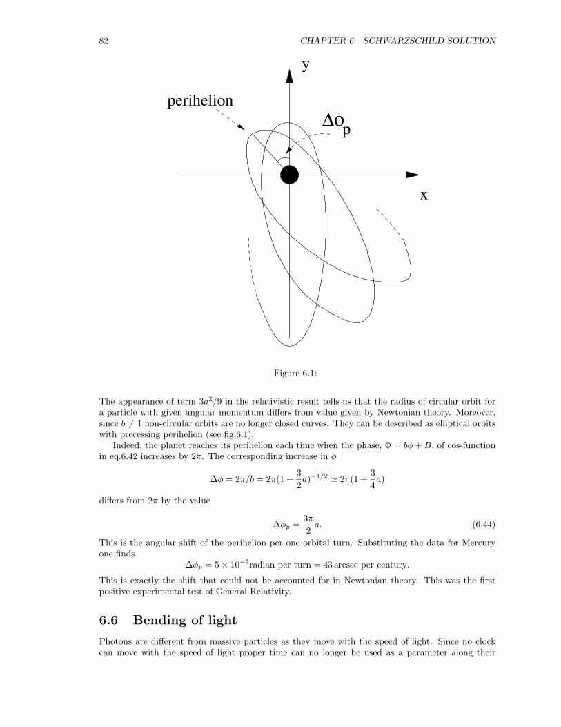
82 CHAPTER 6. SCHWARZSCHILD SOLUTION
∆φperihelion
y
x
p
Figure 6.1:
The appearance of term 3a2/9 in the relativistic result tells us that the radius of circular orbit fora particle with given angular momentum differs from value given by Newtonian theory. Moreover,since b 6= 1 non-circular orbits are no longer closed curves. They can be described as elliptical orbitswith precessing perihelion (see fig.6.1).
Indeed, the planet reaches its perihelion each time when the phase, Φ = bφ+B, of cos-functionin eq.6.42 increases by 2π. The corresponding increase in φ
∆φ = 2π/b = 2π(1− 3
2a)−1/2 ' 2π(1 +
3
4a)
differs from 2π by the value
∆φp =3π
2a. (6.44)
This is the angular shift of the perihelion per one orbital turn. Substituting the data for Mercuryone finds
∆φp = 5× 10⁻⁷radian per turn = 43 arcsec per century.
This is exactly the shift that could not be accounted for in Newtonian theory. This was the firstpositive experimental test of General Relativity.
6.6 Bending of light
Photons are different from massive particles as they move with the speed of light. Since no clockcan move with the speed of light proper time can no longer be used as a parameter along their
6.6. BENDING OF LIGHT 83
world lines. This leads to slight modification in the analysis of their motion. When photons arenon-interacting with other particles this motion is still geodesic and it is still governed by the Euler-Lagrange equations
d
dλ
∂L∂uµ
− ∂L∂xµ
= 0 (6.45)
with the LagrangianL(xν , uν) = gαβ(xν)uαuβ .
However, now λ is just some normal parameter, which we do not have to specify in advance, and
uµ =dxν
dλ
is the corresponding tangent vector to photon’s world-line (null vector). Repeating exactly the samecalculations as those in Sec.6.3 we derive the same results as for massive particles
ut = E = const, (6.46)
uφ = l = const, (6.47)
andd
dλ
(r2dθ
dλ
)− cos θl2
r2 sin3 θ= 0. (6.48)
Just like in the case of massive particles the last equation tells us that the motion of photon is stillplanar and without any loss of generality we may assume that it occurs in the equatorial plane ofSchwarzschild coordinates:
θ = π/2, uθ = 0.
Now ~u is null,gµνu
µuν = 0,
and in Schwarzschild coordinates this reads
gtt(ut)2 + gφφ(uφ)2 + grr(u
r)2 = 0
orgtt(u
t/uφ)2 + gφφ + grr(ur/uφ)2 = 0. (6.49)
Sinceut = gttut = E/gtt,
uφ = gφφuφ = l/gφφ,
ur/uφ = dr/dφ
eq.6.49 reduces tog2φφgtt
(El
)2
+ gφφ + grr
(dr
dφ
)2
= 0.
Substituting expressions for the components of Schwarzschild metric, denoting l/E as b, and intro-ducing new variable
w = rg/r,
which is more convenient in the following calculations, we obtain(dw
dφ
)2
+ w2(1− w)−(rgb
)2= 0. (6.50)
Finally, we differentiate this equation with respect to φ to get
d2w
dφ2+ w − 3
2w2 = 0. (6.51)
84 CHAPTER 6. SCHWARZSCHILD SOLUTION
This second order ODE determines the space trajectory of a photon (w = w(φ) or r = r(φ)), givenits initial position, w(φ0), and initial direction of motion, dw/dφ(φ0). (Given w(φ0) and dw/dφ(φ0)one can find the value of parameter b for this photon from eq.6.50.)
Next we find the perturbative solution for the trajectory of photon in the warped space-time ofthe Sun and show that this trajectory is bend. This bending is just large enough to be measuredusing the technology available at the beginning of the last century.
Let the initial conditions be
w(0) = rg/r(0) = a,dw
dφ(0) = 0 (6.52)
(the latter means that at φ = 0 the photon trajectory is perpendicular to the radial direction). Theclosest distance a photon can get to the Sun is Sun’s radius, r� ' 7 × 1010cm. Sun’s gravitationalradius is much smaller, rg ' 3×105cm. Thus, the highest possible value of a is only about 5×10⁻⁶.This means that we have a small parameter in this problem and can use perturbative approach. Weshell seek solution in the form of asymptotic expansion
w(φ) = aw1(φ) + a2w2(φ) + a3w3(φ) + ... . (6.53)
In fact, we will only find the first two terms in this expansion and ignore the rest as a smallcontribution. Substitute this expression into eq.6.51 and ignore all terms that involve a to the powerof 3 and higher. The result is
aw′′1 + a2w′′2 + aw1 + a2w2 −3
2a2w2
1 = 0. (6.54)
Next we collect terms of the same order in a
a(w′′1 + aw1) + a2(w′′2 + w2 −3
2w2
1) = 0. (6.55)
One can see now that w1 can be found via integrating
w′′1 + aw1 = 0 (6.56)
and then w2 can be found via integrating
w′′2 + w2 −3
2w2
1 = 0. (6.57)
The initial conditions (6.52) and the expansion (6.53) imply the following initial conditions for w1
and w2:
w1(0) = 1, w′1(0) = 0, (6.58)
and
w2(0) = 0, w′1(0) = 0. (6.59)
We are dealing with simple second order linear ODEs. The solution of (6.56,6.58) is
w1(φ) = cosφ,
whereas the solution of (6.57,6.59) is
w2(φ) = 1− 1
2cosφ− 1
2cos2 φ.
Thus, the second order perturbative solution is
w(φ) = a cosφ+ a2(1− 1
2cosφ− 1
2cos2 φ). (6.60)

6.6. BENDING OF LIGHT 85
y
x
δφ δφ
φr
Figure 6.2:
If we kept only the terms of first order in a then we would obtain
r cosφ = rg/a = const.
This describes trajectory which runs parallel to the y-axis in the equatorial plane (see figure 6.2 )and hence shows no bending.
In order to find the magnitude of total bending described by eq.(6.60) consider the limit r =∞or w = 0. Then from eq.(6.60) we find
cosφ = −a1− cos2 φ
1− a/2. (6.61)
Since a� 1, this equation tells us that with great accuracy we can put
cosφ = −a.
The two solutions to this equation can be written as φ = ±(π/2 + δφ) where δφ > 0
sin δφ = a.
Because a� 1 this implies that δφ = a with great accuracy. Then the total bending angle is givenby
∆φ = 2δφ = 2a. (6.62)
For a photon that passes just above Sun’s surface r(0) = r� = 6.97 × 1010cm. This gives us thehighest possible value of a = 4.2× 10⁻⁶ and
∆φ = 1.75arcsec.
In 1919 British astrophysicist A.Eddington confirmed this prediction via observations of backgroundstars during full solar eclipse. The result propelled General Relativity to worldwide recognition.

86 CHAPTER 6. SCHWARZSCHILD SOLUTION
Chapter 7
Appendix
7.1 Geometric units
It is well known that physics needs 3 basic units, for length, time, and mass, and that all other unitscould be derived from these three. Any particular set of units gives certain values for the universalphysical constants, like c, G, and h. However, the universal physical constants allow to reduce thenumber of independent physical units. For example, instead of usual time t one can introduce newtime variable t′ = ct, the geometric time. Obviously, this new time variable will have the dimensionof length,
[t′] = L.
Similarly, instead of usual mass, m, one can introduce the geometric mass, m′ = Gm/c2. It also hasthe dimension of length,
[m′] = L.
Once, we have opted to use geometric time and mass, all other physical quantities get dimensionwhich is a power of L (L0, L, L2 etc.). For example, the dimension of force, which is defined via
f ′ = m′dx
dt′2,
is
[f ′] = LL
L2= L0.
Thus, force becomes dimensionless.Summarizing, the transition to geometric units is described by
t→ t′
c, m→ c2
Gm′. (7.1)
and the inverse transition to generic units is described by
t′ → ct, m′ → G
c2m. (7.2)
These also allow to relate the magnitudes of various physical variables in generic and geometricunits. Take force for example. According to Newton’s definition
f = md2x
dt2=c2
Gm′
d2x
dt′2/c2=c4
Gm′d2x
dt′2=c4
Gf ′.
What can we say about the dimensions of G′ and c′? The dimension of speed in geometric unitsis
[v′] =L
L= L0.
87

88 CHAPTER 7. APPENDIX
Thus, speed becomes dimensionless and so is the speed of light. The dimension of G′ becomesapparent when we inspect Newton’s law of gravity
f ′ = G′m′1m
′2
r2.
Indeed, as we have seen [f ′] = L0 and [m′1m
′2
r2
]=LL
L2= L0.
Thus,[G′] = L0.
The gravitational constant is dimensionless as well.Can we say anything about the values of G and c in geometric units? Yes,
G′ = 1 and c′ = 1. (7.3)
Indeed, in a locally inertial frame in generic units we have
ds2 = −c2dt2 + dl2.
In generic units this reads
ds2 = −c2 dt′2
c2+ dl2 = −dt′2 + dl2.
This tells us that c′ = 1. Next, consider the Newton gravity law
f = Gm1m2
r2.
Converting to geometric units we obtain
c4
Gf ′ = G
m′1(c2/G)m′2(c2/G)
r2=c4
G
m′1m′2
r2.
or
f ′ =m′1m
′2
r2.
This tells us that G′ = 1.


![Tensors, Relativity, And Cosmology [Dalarsson]](https://static.documents.pub/doc/80x56/5695d3cd1a28ab9b029f408d/tensors-relativity-and-cosmology-dalarsson.jpg)