Preprint typeset in JHEP style - HYPER VERSION General Relativity: the Notes * C.P. Burgess Department of Physics & Astronomy, McMaster University, 1280 Main Street West, Hamilton, Ontario, Canada, L8S 4M1. Perimeter Institute for Theoretical Physics, 31 Caroline Street North, Waterloo, Ontario, Canada, N2L 2Y5. Abstract: These notes present a brief introduction to Einstein’s General Theory of Relativity, prepared for the course Physics 3A03. * c Cliff Burgess, March 2009
Transcript
Preprint typeset in JHEP style - HYPER VERSION
General Relativity: the Notes∗
C.P. Burgess
Department of Physics & Astronomy, McMaster University,
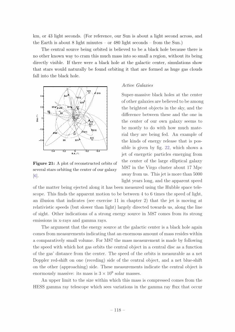
1280 Main Street West, Hamilton, Ontario, Canada, L8S 4M1.
Perimeter Institute for Theoretical Physics,
31 Caroline Street North, Waterloo, Ontario, Canada, N2L 2Y5.
Abstract: These notes present a brief introduction to Einstein’s General Theory
of Relativity, prepared for the course Physics 3A03.
The essence of general relativity is that gravity is described by the geometry of
spacetime, and so this first section pauses to summarize some of the mathematics
used to describe non-Euclidean geometries. Before doing so, a brief reminder about
Euclidean geometry.
Euclidean Geometry
Euclid founded his study of plane (i.e. 2-dimensional) geometry on the following five
axioms:
1. Any two points can be joined by a straight line.
2. Any straight line segment can be extended indefinitely in a straight line.
3. Given any straight line segment, a circle can be drawn having the segment as
radius and one endpoint as center.
4. All right angles are congruent.
5. Parallel postulate: If two lines intersect a third in such a way that the sum of
the inner angles on one side is less than two right angles, then the two lines
inevitably must intersect each other on that side if extended far enough.
All of these seem to be obviously true, given the standard notions of what a point,
straight line, circle, right angle and congruence mean. Among the consequences of
these axioms are many familiar statements like: the ratio of a circle’s circumference,
C, to its radius, r, is a universal number: C/r = 2π; the ratio of a circle’s area,
A, to the square of its radius is also a universal number A/r2 = π; the sum of the
interior angles of a triangle sum to 180 degrees, and so on. We are used to taking
– 2 –
these consequences for granted when understanding the relations amongst objects in
physical space.
The rest of this section is devoted to describing simple situations where they
do not all apply. Once this is done, it becomes an experimental issue whether or
not the Euclidean axioms are properties of the space in which we find ourselves
situated. The goal of this section is to develop the tools for this, by setting up a
precise characterization of these new geometries, and the ways they can differ from
Euclidean space.
1.1 The Geometry of Surfaces
The non-Euclidean geometries that are easiest to visualize are those of two-dimensional
surfaces, such as planes, spheres or hyperbolae. These are easy to picture since we
can envision these surfaces embedded in 3-dimensional space.
To this end consider the 3-dimensional vector space, IR3, whose vectors, r, de-
scribe the distance from an (arbitrary) origin, O, to the various points in space. It
is convenient to describe such a vector by its components referred to a ‘rectangular’
basis of unit vectors, ex, ey, ez, oriented in a fixed but arbitrary direction, so that
r = x ex + y ey + z ez
= xi ei , (1.1)
where the three coordinates, (x, y, z), each can run from −∞ to ∞.
Some important notation is introduced in the second equality of eq. (1.1), which
writes x1 = x, x2 = y, x3 = z, and e1 = ex, e2 = ey and e3 = ez. There is
also an implied sum from 1 to 3 over the repeated index ‘i’, or any other repeated
index taken from the middle of the Latin alphabet for that matter. (Indices taken
from the beginning of the Latin alphabet are encountered later, where they run over
a, b = 1, 2; and indices from the Greek alphabet also come up, and will be summed
from µ, ν = 0, 1, 2, 3.) This rule for summing over repeated indices is called the
Einstein summation convention, and in terms of it the dot product of two vectors
with components a = ai ei and b = bi ei can be written a · b = δij aibj, where the
Kronecker-δ symbol has the property that δij = 1 if i = j and δij = 0 otherwise.
We take the distance, s(r1, r2), between any two points, r1 and r2, in IR3 is given
in terms of their rectangular coordinates by the usual Pythagorean rule
s(r1, r2) = |r1 − r2| =√
(r1 − r2) · (r1 − r2)
=
√δij(xi1 − xi2)(xj1 − x
j2) (1.2)
=√
(x1 − x2)2 + (y1 − y2)2 + (z1 − z2)2 ,
– 3 –
where the middle line again uses the Einstein summation convention. This definition
has the important property that it does not depend at all on the origin, O, and
orientation of the axes, ei = ex, ey, ez, that are required to define the coordinates
xi = x, y, z describing r1 and r2.
Curves in Space
Before describing two-dimensional surfaces in IR3, it is worth briefly digressing to
describe the simpler case of one-dimensional curves. A curve in IR3 is defined by the
locus of points that are swept out as a single parameter varies:
r(u) = x(u) ex + y(u) ey + z(u) ez
= xi(u) ei . (1.3)
Here the parameter u labels the points on the curve and our interest is usually in
component functions xi(u) = x(u), y(u), z(u) that are multiply differentiable with
respect to u.
For example, straight lines in this picture are described by linear functions,
r(u) = a + bu, where a and b are arbitrary constant vectors. When the origin, O,
is not on the straight line (i.e. a 6= 0) then the origin together with the line define
a plane, which is spanned by the vectors a and b. More generally, a straight line is
also given by r(u) = a + b f(u), for any function f(u) that satisfies df/du 6= 0, since
this simply represents a relabelling of the points along the curve.
By contrast, a curve of the form r(u) = c + a cosu + b sinu traces out a more
complicated closed shape, which becomes an ellipse if a and b are perpendicular to
one another: a · b = axbx + ayby + azbz = 0. In this case c specifies the position of
the ellipse’s centre, and its two semi-major axes are
a = |a| =√
a · a =√a2x + a2
y + a2z =
√δij aiaj
b = |b| =√
b · b =√b2x + b2
y + b2z =
√δij bibj . (1.4)
This ellipse is inscribed on the plane spanned by the vectors a and b, and degenerates
into a circle in the special case that a and b have the same length: a = b.
The family of vectors that lie tangent to a curve r(u) is found by differentiation,
t(u) =dr
du=
dx
duex +
dy
duey +
dz
duez =
dxi
duei , (1.5)
and a one-parameter family of unit vectors tangent to the curve is found by normal-
izing
et(u) =t(u)
|t(u)|, (1.6)
– 4 –
so et · et = 1 for all u. For a straight line, r(u) = a + bf(u), the tangent
t(u) =dr
du= b
df
du, (1.7)
has a constant direction, but a u-dependent length that depends on the precise
function f(u) used to parametrize the curve. But for any parametrization the unit
tangent vector for a straight line is a constant vector: et = b/|b|. The basis vectors,
ei = ex, ey, ez may themselves be regarded as unit tangent vectors to the curves
defining the rectangular coordinate axes themselves: that is, ex is the unit tangent
to the curves along which y and z are constant, and similarly for ey and ez.
The tangent to the elliptical curve centered at the origin, r(u) = a cosu+b sinu
is given by t(u) = −a sinu + b cosu, whose direction changes continuously with u,
with norm |t(u)| =√a2 sin2 u+ b2 cos2 u (and we use a ·b = 0). In this case the unit
tangent is et(u) = (−a sinu+ b cosu)/|t(u)|. Notice that the inner product between
the radius vector and the tangent is t(u) · r(u) = (b2− a2) sinu cosu, which vanishes
for all u in the case of a circle, where b = a.
Distances along curves
Measures of length and angle play a central role in geometry, and since angle (in
radians) is defined in terms of ratios of lengths, the basic problem is how to measure
length within curved surfaces. This section describes a first step in this direction:
measuring length along curves.
The starting point is eq. (1.2), telling us how distances are measured in IR3. We
apply this to find the distance, ds, between two points on a curve, r(u) and r(u+du),
that are infinitesimally far from one another.
ds = |r(u+ du)− r(u)| =∣∣∣∣dr
du
∣∣∣∣ du =
√dr
du· dr
dudu =
√δij
dxi
du
dxj
dudu , (1.8)
The arc-length along a finite-sized interval of the curve is then obtained by integration
s(u1, u2) =
∫ u2
u1
du
√δij
dxi
du
dxj
du. (1.9)
For example, for the circle r(u) = a(ex cosu+ey sinu) we have dr/du = a(−ex sinu+
ey cosu) and so ds = a du, giving s(u1, u2) = a(u2 − u1).
Arc-length provides a particularly physical way to parameterize a curve. Once
this is done the tangent vector to a curve is automatically a unit vector. To see this
consider a generic curve, r(u), defined using a generic parameter, u. The tangent
vector computed using arc-length as a parameter is
dr
ds=
dr
du
du
ds=
t
|t|= et , (1.10)
where t = dr/du and eq. (1.8) is used to evaluate du/ds = 1/|t|.
– 5 –
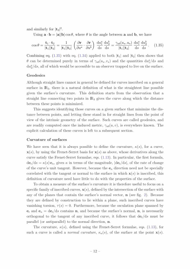
Curvature of curves
Figure 1: The Frenet-Serret basis vectors
and the osculating plane (Wikipedia).
In addition to the unit tangent, et =
dr/ds, there is also a natural family of
orthonormal basis vectors that can be
defined everywhere along a curve. A unit
vector, n, that is always perpendicular
to et is found as above by differentia-
tion with respect to arc length: n(s) =
det/ds. The fact that this definition gives
a vector normal to et can be seen by dif-
ferentiating the condition et · et = 1, as
follows:
et · n = et ·detds
=1
2
d
ds
(et · et
)= 0 .
(1.11)
The plane spanned by t(s) and n(s) at
each u is called the osculating plane for
the curve r(s). The vectors
et(s) , en(s) =n(s)
|n(s)|and the cross product eb(s) = et(s)× en(s) , (1.12)
give an orthonormal triad of vectors at each point along the curve, one of which is
always tangent.
Because these vectors form a basis, their derivative along the curve can be ex-
panded in terms of them, leading to:
detds
= κ en
dends
= −κ et + τ eb (1.13)
debds
= − τ en .
These expressions are known as the Frenet-Serret formulae, and the basis et, en
and eb is called the Frenet-Serret basis. The coefficients in this expression give a
differential measure of the curvature, κ(s), and torsion, τ(s), at each point of the
curve r(s).
Exercise 1: Use the definitions of et, en and eb to prove that only
two parameters, κ and τ , are required to label their derivatives as in
eqs. (1.13).
– 6 –
Notice that the definitions show that κ = τ = 0 for a straight line. Conversely,
if κ and τ vanish for all u, then eqs. (1.13) can be integrated twice to show that the
corresponding curve, r(u), is a straight line. Similarly, if τ should vanish for all u
(with κ(u) arbitrary), then the curve must be confined to the plane that is normal
to the constant vector eb.
Exercise 2: Show that the curvature and torsion of the curve r(s) =
a[ex cos(s/a) + ey sin(s/a)] (a circle of radius a) are constant, with κ =
1/a and τ = 0. Repeat for the helical curve r(u) = a(ex cosu+ey sinu)+
` u ez, keeping in mind that the arc-length in this case satisfies s =
u√a2 + `2.
Surfaces in IR3
A two-dimensional surface embedded in IR3 is similarly defined by the locus of points
swept out by a two-parameter family,
r(u, v) = xi(u, v) ei = x(u, v) ex + y(u, v) ey + z(u, v) ez . (1.14)
Alternatively, it is sometimes more convenient to define the surface implicitly, rather
than explicitly, such as through an algebraic condition of the form f(r) = 0. In this
case the expression r(u, v) can be regarded as being obtained as the solution to this
condition. We next provide explicit representations for some simple surfaces, many
of which are used as illustrative examples in later sections.
Planar surfaces:
A plane passing through the origin and spanned by two linearly-independent
vectors a and b is swept out by a surface whose equation has the form
r(u, v) = au+ b v , (1.15)
with −∞ < u, v < ∞. Straight lines can be inscribed inside such a plane, such as
r(u) = au or r(v) = b v or r(u) = (a + b)u, as can circles. As is easily verified, the
geometry of these circles and straight lines defined for any such a plane satisfies the
axioms of Euclidean geometry.
Planes can equally well be specified through a constraint f(r) = 0. For example,
the plane r(u, v) = ex u+ ey v defined by the x- and y-axes is equally well described
as the general solution to the condition z = 0, and so f(r) := z = ez · r.
Cylindrical surfaces:
A slightly more interesting example is provided by a cylindrical surface. A rep-
resentation for a cylinder concentric with the z-axis and having an elliptical profile
– 7 –
aligned with the x- and y-axes would be
r(u, v) = ex a cosu+ ey b sinu+ ez v , (1.16)
where 0 ≤ u < 2π and −∞ < v <∞. The constants a and b define the semi-major
axes of the elliptical cross sections taken at fixed z. This elliptical cylinder could
equally well be specified by the condition f(r) := (x2/a2) + (y2/b2) − 1 = 0. It is
possible to inscribe straight lines on such a cylinder, but only if they are parallel
with the z-axis: for instance r(v) = ex a cosu? + ey b sinu? + ez v, where u? is any
particular, fixed, value of u.
Spherical surfaces:
The surface of a sphere provides an example of a truly curved surface (in a
sense explained in detail below). A representative sphere centered at the origin with
radius a can be represented as the surface f(r) := x2 + y2 + z2− a2 = 0, or explicitly
parameterized using spherical polar coordinates (u = θ and v = φ) by:
r(u, v) = ex a sinu cos v + ey a sinu sin v + ez a cosu , (1.17)
with 0 < u < π and 0 ≤ v < 2π. It is intuitively clear that no straight lines can be
inscribed on a sphere.
Inscribed Curves
Given a surface r(u, v) = xi(u, v) ei in IR3, an inscribed curve is a curve, x(w) =
xi(w) ei, in IR3 whose points also lie within the surface. For instance if the surface
is defined by a condition of the form f(r) = 0, then an inscribed curve satisfies
f(x(w)) = 0 for all values of its parameter, w. An alternative way of describ-
ing an inscribed curve is to specify the curve parameters, u(w), v(w), that trace
out the points along the curve: r((u(w), v(w)) = x(w). For instance, the circle
x(w) = a(ex cosw + ey sinw) is inscribed in the sphere r(u, v) = a(ex sinu cos v +
ey sinu sin v+ez cosu), and can be described by the parameter values u(w), v(w) =
π2, w.
The tangent to an inscribed curve can therefore be written either in terms of
derivatives of x(w) or r(u, v),
t =dx
dw=
d
dwr(u(w), v(w)) =
∂r
∂u
du
dw+∂r
∂v
dv
dw. (1.18)
It is useful to use the Einstein summation convention to combine the above expres-
sions into the more compact notation
t =∂r
∂uadua
dw=∂xi
∂uadua
dwei , (1.19)
– 8 –
where a = 1, 2 with u1 = u and u2 = v.
A particularly simple family of inscribed curves is obtained by holding fixed either
one of the two parameters, u or v, that define the surface itself. Consider for instance
a surface defined by the locus of points swept out by a particular parameterization
r(u, v). A family of curves lying in this surface, parameterized by u, is found by
setting v to some fixed value v = v?: r(u) = r(u, v?). Different values of v? produce
different members of this family of curves. A second family of curves lying within
r(u, v) is similarly obtained by fixing u at a sequence of values, u = u?, and letting
the variation of v parameterize the curves: r(v) = r(u?, v). Different choices for u?
then define different members of this family of curves.
It is possible to use the tangents of inscribed curves to define a pair of linearly
independent tangent vectors to any surface that are not necessarily orthogonal. These
are given above simply by computing the tangent vector for the inscribed curves along
which only one of either u or v varies. The tangent to the curves along which only
u varies is given by
t(u) =∂r
∂u(u, v?) , (1.20)
and a family of unit vectors tangent to these curves are then given by eu = t(u)/|t(u)|.The tangents to the curves along which only v varies are similarly given by
t(v) =∂r
∂v(u?, v) , (1.21)
and the unit tangent becomes ev = t(v)/|t(v)|.Again using the notation ua = u1, u2 = u, v, these may be written
ta =∂r
∂ua=∂xi
∂uaei , (1.22)
where t1 = t while t2 = t. The span of the normalized vectors ea(u, v) define the
tangent plane to the surface at the point labelled by (u, v).
A normal vector defined everywhere on the surface r(u, v) may then be con-
structed using the two families of tangent vectors defined above, eu and ev, by taking
the cross product: en(u, v) = eu(u, v)× ev(u, v). This defines a basis of vectors that
is adapted to the surface at every point.
Notice that if the surface is specified by a constraint, f(r) = 0, then an alternative
way to identify this normal direction is by taking the gradient of f :
n = ∇f = ex
(∂f
∂x
)+ ey
(∂f
∂y
)+ ez
(∂f
∂z
), (1.23)
because the following argument shows this vector is orthogonal to the tangent vectors.
The argument relies on the observation that if r(u, v) is a parametrization of the
– 9 –
surface defined by f(r) = 0, then what this means is f(r(u, v)) = 0 for all u and v.
Differentiating this last expression with respect to u or v, and using the chain rule,
then implies ∇f · (∂r/∂u) = ∇f · (∂r/∂u) = 0, or
ta · ∇f =∂r
∂ua· ∇f =
∂xi
∂ua∂if =
∂x
∂ua∂f
∂x+
∂y
∂ua∂f
∂y+
∂z
∂ua∂f
∂z= 0 , (1.24)
which states that ∇f is perpendicular to both the tangent vectors, ta = t, t.Eq. (1.24) introduces the notation
∂i :=∂
∂xi, (1.25)
and (for practice) is rewritten several ways to emphasize the Einstein summation
convention.
Distances along surfaces
Distances along a surface are similarly measured along a curve inscribed in this
surface, and in general the distance between two points depends on the details of
which curve is used to link these points, just as is also true for points in IR3.
In IR3 when one speaks of the distance between two points without referring to
the curve involved, what is meant is the distance along the straight line that connects
the two points. Since a straight line cannot in general be inscribed into a generic
curved surface it is clear that the same definition cannot generically be used to define
a distance between points in a generic surface.
An exception to this is when the two points of interest are infinitesimally sepa-
rated on the surface: r(u, v) and r(u+ du, v+ dv), since in this case the straight-line
curve that connects them is arbitrarily close to an inscribed arc lying on the surface.
In this case the distance between the points becomes
ds = |r(u, v)− r(u+ du, v + dv)| =∣∣∣∣ ∂r
∂uadua∣∣∣∣ =
√δij
∂xi
∂ua∂xj
∂ubdua dub . (1.26)
The last version of this equation, using the Einstein summation convention, is most
commonly written without the ugly square root:
ds2 = γab(u, v) duadub , (1.27)
where the right-hand side defines what was historically called the surface’s first fun-
damental quadratic form — or its induced metric in more modern parlance — with
γab = δij∂xi
∂ua∂xj
∂ub. (1.28)
A central point of the geometry of surfaces is that any intrinsic property of the
surface — that is, involving only distances and angles associated to inscribed curves
on the surface — can be expressed in terms of γab(u, v) and its derivatives.
– 10 –
Exercise 3: Show that the induced metric for the plane given by r(u, v) =
ex u+ ey v in IR3 is
γab = δab =
(1 0
0 1
), (1.29)
where δab is the Kronecker δ-function, defined just above eq. (1.2). Repeat
the calculation for the cylinder r(u, v) = a(ex cosu + ey sinu) + ezv to
show that
γab =
(γuu γuv
γvu γvv
)=
(a2 0
0 1
). (1.30)
Finally repeat for the sphere r(u, v) = a(ex sinu cos v + ey sinu sin v +
ez cosu), to show
γab =
(γuu γuv
γvu γvv
)=
(a2 0
0 a2 sin2 u
). (1.31)
The arc-length along any inscribed curve running between points A and B may
now be found by integrating eqs. (1.27) in the form:
s(A,B) =
∫ wB
wA
dwds
dw=
∫ wB
wA
dw
√γab(w)
dua
dw
dub
dw, (1.32)
where γab(w) = γab(u(w), v(w)).
Angles between inscribed curves
The angle, θ, between two inscribed curves that intersect at a point P can also be
computed using γab evaluated at P .
To see this suppose the curves x1(s) and x2(s) inscribed in the surface r(u, v)
intersect at the point labelled by (u, v) = (u?, v?). The angle between these curves
may be defined as the angle between their tangent vectors, evaluated at P :
t1 =dx1
ds=
∂r
∂uadua1ds
, (1.33)
where ua1(s) = u1(s), v1(s) describes the parameters which describe the locus of
points on the surface through which the inscribed curve x1(s) = r(u1(s), v1(s)) passes.
An identical expression also holds for t2 = dx2/ds and ua2(s) = u2(s), v2(s). Clearly
the norm of the tangent vector evaluated at P is therefore given by
|t1|2 =dx1
ds· dx1
ds=
∂r
∂ua∂r
∂ubdua1ds
dub1ds
= γab(u?, v?)dua1ds
dub1ds
, (1.34)
– 11 –
and similarly for |t2|2.
Using a · b = |a||b| cos θ, where θ is the angle between a and b, we have
cos θ =t1 · t2
|t1||t2|=
1
|t1||t2|
(∂r
∂ua· ∂r
∂ub
)dua1ds
dub2ds
=γab(u?, u?)
|t1||t2|dua1ds
dub2ds
. (1.35)
Combining eq. (1.35) with eq. (1.34) applied to both |t1| and |t2| then shows that
θ can be determined purely in terms of γab(u?, v?) and the quantities dua1/ds and
dua2/ds, all of which would be accessible to an observer trapped to live on the surface.
Geodesics
Although straight lines cannot in general be defined for curves inscribed on a general
surface in IR3, there is a natural definition of what is the straightest line possible
given the surface’s curvature. This definition starts from the observation that a
straight line connecting two points in IR3 gives the curve along which the distance
between these points is minimized.
This suggests identifying those curves on a given surface that minimize the dis-
tance between points, and letting these stand in for straight lines from the point of
view of the intrinsic geometry of the surface. Such curves are called geodesics, and
are readily computed once the induced metric, γab(u, v), is everywhere known. The
explicit calculation of these curves is left to a subsequent section.
Curvature of surfaces
We have seen that it is always possible to define the curvature, κ(s), for a curve,
x(s), by using the Frenet-Serret basis for x(s) as above, whose derivatives along the
curve satisfy the Frenet-Serret formulae, eqs. (1.13). In particular, the first formula,
det/ds = κ(s) en, gives κ in terms of the magnitude, |det/ds|, of the rate of change
of the curve’s unit tangent. However, because the en direction need not be specially
correlated with the tangent or normal to the surface in which x(s) is inscribed, this
definition of curvature need have little to do with the properties of the surface.
To obtain a measure of the surface’s curvature it is therefore useful to focus on a
specific family of inscribed curves, x(s), defined by the intersection of the surface with
any of the planes that contain the surface’s normal vector, n (see fig. 2). Because
they are defined by construction to lie within a plane, such inscribed curves have
vanishing torsion, τ(s) = 0. Furthermore, because the osculation plane spanned by
et and en = det/ds contains n, and because the surface’s normal, n, is necessarily
orthogonal to the tangent of any inscribed curve, it follows that det/ds must be
parallel (or antiparallel) to the normal direction, n.
The curvature, κ(s), defined using the Frenet-Serret formulae, eqs. (1.13), for
such a curve is called a normal curvature, κn(s), of the surface at the point x(s).
– 12 –
Figure 2: Illustration of several planes whose intersection with a surface define the curves
whose curvature is a normal curvature (Wikipedia).
These are not unique, since they depend on the direction of the plane containing n
that is used in the construction. The surface’s principal curvatures, κ1 and κ2, are
defined at each point as the maximum and minimum values taken by the normal
curvatures as the direction of this plane is varied.
The surface’s mean curvature, H, and Gaussian curvature, K, are then defined
as the arithmetic and geometric means of κ1 and κ2:
H =1
2(κ1 + κ2) and K = κ1κ2 . (1.36)
Although it is not clear from its definition, Gauss’ Theorema Egregium states that
the Gaussian curvature can be determined purely in terms of lengths and angles
measured within the surface — that is, in terms of the induced metric γab and its
derivatives — and so is a property intrinsic to the surface itself (as opposed to an
extrinsic property that depends on how the surface is embedded into the external
IR3).
Exercise 4: Show that the principal curvatures for the plane r(u, v) =
ex u+ey v are κ1 = κ2 = 0. Repeat for the cylinder r(u, v) = a(ex cosu+
ey sinu) + ezv to show they are κ1 = 0 and κ2 = 1/a. Finally, show that
for the sphere r(u, v) = a(ex sinu cos v + ey sinu sin v + ez cosu), the
principal curvatures are equal and positive: κ1 = κ2 = 1/a.
– 13 –
Changing the parametrization
Notice that the discussion so far did not need to provide any details about the
kinds of parameters, (u, v), used to specify the surface. Before generalizing the
above discussion to more general spaces, it is worth first digressing briefly about how
quantities change as the coordinates used to describe them change.
Contravariant vectors
When describing a surface, r(u, v), we saw that the inscribed curves along which
the parameters ua = u, v vary could be used to provide a natural basis, ta =
∂r/∂ua, for the surface’s tangent plane. Because this forms a basis, it can be used
to define the components of any vector at all that is tangent to the surface:
c = ca ta = cu tu + cv tv , (1.37)
Suppose we now change our parametrization of the surface, defining new pa-
rameters ua′(u, v) = u′(u, v), v′(u, v) that provide equally good labels for points
on the surface: r(u, v) = r(u′(u, v), v′(u, v)). Provided that the new parameters are
really independent of one another (more about this below), the tangents to these
new parameter curves define a new basis, ta′ = ∂r/∂ua′, of the same tangent plane,
in terms of which the same vector c has the expansion
c = ca′ta′ = cu
′tu′ + cv
′tv′ . (1.38)
To obtain the relation between the coefficients ca′
and ca we relate the two sets
of tangent bases to one another, using the chain rule:
ta =∂r
∂ua=∂ua
′
∂ua∂r
∂ua′=∂ua
′
∂uata′ , (1.39)
and so
c = ca ta = ca∂ua
′
∂uata′ (1.40)
which implies
ca′= ca
∂ua′
∂ua. (1.41)
Components ca that transform in this way under a change of parametrization are
called contravariant components, and c would be called a contravariant vector.
An earlier-mentioned proviso to this discussion was the requirement that the new
coordinates be independent of one another and so provide a faithful parametrization
of the surface. Eq. (1.39) provides a local criterion for when this is so, since it is
equivalent to asking when the new pair of tangent vectors are linearly independent of
– 14 –
one another (as is required if they are to form a basis). Since eq. (1.39) can equally
well be written in matrix notation as
t = J t′ , (1.42)
with
t =
(tu
tv
), t′ =
(tu′
tv′
)and J =
(∂u′/∂u ∂v′/∂u
∂u′/∂v ∂v′/∂v
), (1.43)
the new basis is linearly independent if and only if the matrix J is invertible, or
equivalently if its determinant, J = det J — the Jacobian of the transformation
(u, v)→ (u′, v′) — is nonzero: J 6= 0.
Covariant Vectors
There is an alternative way of using parameters on a surface to describe vectors
that are tangent to the surface. Instead of defining a set of basis vectors that are
tangent to lines along which one parameter varies, ta = ∂r/∂ua = (∂xi/∂ua) ei, one
can instead define a basis of vectors, sa, using the normals to the surfaces along
which one of the parameters is held constant. That is we ask the basis sa to satisfy
the defining condition
sa · tb = δab , (1.44)
where, as before, the Kronecker symbol satisfies δab = 1 if a = b and vanishes
otherwise. Such a basis is often called a basis dual to the basis of tangent vectors.
Although these two definitions give the same bases
Figure 3: An example where
normals to coordinate surfaces
(small arrows) are not equiva-
lent to tangents to coordinate
directions (lines).
in many of the simple coordinates commonly used
(like rectangular or polar coordinates), they need not
always do so. An example of an ‘oblique’ set of coor-
dinates, where these two definitions would not agree,
is given by the parameters on a plane defined by
r(u, v) = au + b v, when the vectors a and b are
not orthogonal to one another. A cartoon of these
coordinates is given in figure 3. In general curvi-
linear coordinates both bases are possible, and most
importantly, transform differently when the surface
is reparameterized (u, v)→ (u′v′).
Since the sa form a basis for the surface’s tangent
plane, a general vector, c, tangent to the surface can be expanded
c = cb sb , (1.45)
– 15 –
and the coefficients in this expansion are given by
c · ta = cb sb · ta = cb δba = ca . (1.46)
These components change if the parameters used to label the surface are changed,
(u, v)→ (u′(u, v), v′(u, v)), but in a different way than did the components ca arising
when c is expanded directly in terms of the ta’s. Using eq. (1.39) with eq. (1.46)
gives
ca′ = c · ta′ =∂ub
∂ua′c · tb =
∂ub
∂ua′cb , (1.47)
where we use that the partial derivatives ∂ub/∂ua′make up the elements of the matrix
J−1 that is inverse to the matrix J whose elements are ∂ua′/∂ub. Equivalently, using
the Einstein summation convention we use the identity
∂ub
∂ua′∂ua
′
∂uc= δbc and its partner
∂ub′
∂ua∂ua
∂uc′= δb
′c′ . (1.48)
Coefficients that transform as in eq. (1.47) are said to transform as covariant com-
ponents.
Tensors
Since the first fundamental form, γab, is so central to the geometry on a surface,
it is worth knowing how it transforms when the parameters labelling the surface
are changed. Keeping in mind its definition in terms of the distance, ds, along the
surface, eq. (1.27), and recognizing that a physical quantity like ds must be parameter
independent shows that if (u, v)→ (u′, v′), then the chain rule implies
ds2 = γab duadub = γab∂ua
∂uc′∂ub
∂ud′duc
′dud
′, (1.49)
which shows
γc′d′(u′, v′) = γab(u(u′, v′), v(u′, v′))
∂ua
∂uc′∂ub
∂ud′. (1.50)
Since this looks like two copies of the transformation rule, eq. (1.47), the quantity
γab is said to transform like a covariant tensor of rank 2.
More generally, if something having many indices transforms under a change of
parameters like
T a′1..a′kb′1..b
′`(u′, v′) = T c1..ckd1..d`(u(u′, v′), v(u′, v′))
∂ua′1
∂uc1· · · ∂u
a′k
∂uck∂ud1
∂ub′1· · · ∂u
d`
∂ub′`
,
(1.51)
is called a tensor of covariant rank ` and contravariant rank k. The special case
of something which has no indices, such as an inner product between two vectors
tangent to a surface,
m · n = (ma ta) · (nb tb) = manb∂r
∂ua· ∂r
∂ub= γabm
anb , (1.52)
– 16 –
transforms according to
γa′b′ma′nb
′=
(γcd
∂uc
∂ua′∂ud
∂ub′
)(me ∂u
a′
∂ue
)(nf
∂ub′
∂uf
)= γef m
enf , (1.53)
(which uses eq. (1.48) twice) and is called a scalar.
The reason tensors like this are important is that physical laws cannot depend
on our arbitrary choice of how we parameterize a surface. A physical statement
— like F = m a, say — directly relates physical objects, like vectors, distances or
inner products. And although the components of each quantity like F, m and a
can individually change when different parameters or bases are used, it is always
true that both sides of the equality transform in precisely the same way. Thus it is
important for Newton’s Law that F and the product of m times a both transform
as vectors.
We similarly demand on curved space that any reasonable physical law must have
the form A = B, where both sides of the equation are tensors of precisely the same
type. This ensures that once we know the components Aa1..ak b1..b` and Ba1..akb1..b` are
equal in a particular basis, it is automatic that they will also be equal in any other
basis we should choose to examine.
1.2 More General Curved Space
We are now ready to kick away the crutch of embedding surfaces into flat IR3 and
formulate directly what non-Euclidean geometry might look like in three (or more)
dimensions. The key in doing so is to focus on those relations derived above for
surfaces that do not make any reference at all to how the surface is situated within
its embedding space.
Tensors and Curvilinear Coordinates
We start by choosing an arbitrary set of coordinates, xi, to label the points in three di-
mensions, without requiring that these coordinates be the usual rectangular x, y, z.For instance we could instead use spherical polar coordinates xi = r, θ, φ, or any
other choice of coordinates which happens to suit our purposes.1
Just as for surfaces we can also define curves ‘inscribed’ within our space by
specifying how the coordinates vary along the curve: xi(u) = x1(u), x2(u), x3(u).At each point P in our three-dimensional space we can define a tangent space, TP —
1As a technical point, it is not necessary that any one choice of coordinates describe all of the
points in space. It is sufficient to have a collection of coordinate choices which cover the entire
space once taken together, with sufficient overlap between pairs of coordinate patches to allow the
results of measurements to be translated from one set of coordinates to another.
– 17 –
i.e. a generalized tangent plane — comprising the vector space spanned by all of the
tangents at P to the curves that pass through P .
A choice of coordinates provides a natural basis for describing vectors that lie
within the tangent space at each point. This can be taken to be defined by the vectors
ti that are tangent to the curves along which only one of the coordinates varies.
Notice that this basis need not be normalized or mutually orthogonal, although it
must be linearly independent and complete.
In terms of the basis ti, the tangent, t, to any other curve defined by xi(w) has
components
t =dxi
dwti . (1.54)
These components define a contravariant vector, in the sense that if we change co-
ordinates from xi to xi′, the components t in the new basis vectors, ti′ , are given
bydxi
′
dw=∂xi
′
∂xjdxj
dw. (1.55)
Such a coordinate transformation is only well-defined if the matrix whose entries are
∂xi′/∂xj is invertible.
A contravariant tensor, T, having rank p is similarly defined to have components
involving p indices, that transform under a coordinate change according to
T i′1..i′p(x′) = T j1..jp(x(x′))
∂xi′1
∂xj1· · · ∂x
i′p
∂xjp. (1.56)
Metrics
We now come to the central concept. The essence of the geometry is determined
by specifying a notion of distance between points within the space. This is done
by giving the metric, gij(x) = gji(x), which is a symmetric three-by-three positive-
definite matrix whose entries are a function of position. gij(x) is defined to give the
distance between two infinitesimally displaced points, situated at xi and xi + dxi, as
ds =√gij(x) dxi dxj . (1.57)
The square root is always real because gij is positive definite, and ds = 0 only occurs
if dxi = 0. This last equation is more commonly written without the square root as
ds2 = gij(x) dxi dxj . (1.58)
Besides providing a notion of distance, the metric provides a natural way to define
the angle between two curves. This is done by using the metric to define an inner
product between the tangent vectors of the two curves at their point of intersection.
That is, suppose the curves xi1(u) and xi2(v) both pass through the point P , then
– 18 –
their tangent vectors, m1 and m2 respectively have components dxi1/du and dxi2/dv.
Guided by eq. (1.35), we can then define the intersection angle between the two
curves as
cos θ =m1 ·m2√
(m1 ·m2)(m2 ·m2), (1.59)
evaluated at P , where the inner product is defined in terms of the vector components
as
a · b = gij ai bj . (1.60)
Notice that in particular the inner product of the tangents of the two curves xi1(u)
and xi2(v) becomes
m1 ·m2 = gijdxi1du
dxj2dv
, (1.61)
and so in particular, for basis vectors defined as tangents to the coordinate lines
themselves we have
ti · tj = gij . (1.62)
Having a notion of angles also means we know what it means for vectors to be
orthogonal: a · b = 0. This then allows the definition of the second natural basis for
vectors, si, in terms of the normals to the surfaces on which one coordinate is held
fixed. Such a dual basis must satisfy si · tj = δij, and so if a vector m is expanded
m = mi ti and m = mi si, then the components are given by
mi = m · ti = (mj tj) · ti = mj gij . (1.63)
It is convenient to define the quantities gij as the components of the matrix
that is inverse to the matrix whose components are gij. Such a matrix always exists
because the fact that gij is positive definite excludes the possibility of it having a
zero eigenvector, and so not having an inverse. With this definition we have
gij gjk = δik , (1.64)
and so multiplying eq. (1.63) by gik (including the implied sum over i, from the
Einstein summation convention) gives
mk = gkimi . (1.65)
Notice that its definition, together with the invariance of the distance element,
ds, implies that under a coordinate transformation gij transforms as
gi′j′ = gkl∂xk
∂xi′∂xl
∂xj′, (1.66)
– 19 –
what is called the transformation of a covariant tensor of rank 2. Similarly the
covariant components, mi, of a vector m transform as (compare with eq. (1.56))
mi′ = mj∂xj
∂xi′, (1.67)
which is a covariant tensor of rank 1, or one-form. The transformation properties of
covariant tensors of higher rank can be similarly defined.
Geodesics
Returning to the main line of development, following the example of curves on a sur-
face, we now define a geodesic as the curve that minimizes the distance between two
points. Such curves are the natural generalization of the straight lines of Euclidean
geometry.
To determine the local equations that govern geodesics, we must first find an
expression for the distance between two points, A and B, that is to be minimized.
If this distance is measured along a curve, xi(u), that connects them, the distance
may be found by integrating the infinitesimal definition, eq. (1.57), in the form
sAB =
∫ uB
uA
duds
du=
∫ uB
uA
du
√gij(x(u))
dxi
du
dxj
du=
∫ uB
uA
du√gij(x(u)) xi xj .
(1.68)
This introduces the simplifying notation xi := dxi/du.
If xi(u) were the curve of minimum length, then the quantity sAB should be
stationary with respect to small changes, xi(u) → xi(u) + δxi(u), to the curve, at
least to first order in δxi(u). Such variations must vanish in the same way that small
changes to a function, f(x), vanish to linear order in δx if they are evaluated at a
function’s minimum, x = xm: f(xm + δx)− f(xm) ' f ′(xm) δx = 0. The conceptual
difference here is that the length sAB is a functional that depends on the shape of
the entire curve, xi(u), and not simply on its value at a single point, like A or B.
To see what it means for sAB to be stationary, let us write it as sAB[x(u)],
to emphasize that it depends on the shape of the curve xi(u) in addition to the
endpoints. We then evaluate the difference, δsAB = sAB[x(u)+δx(u)]−sAB[x(u)], and
expand the result out to linear order in δxi(u), using gij(x(u) + δx(u)) ' gij(x(u)) +
δxk(u) ∂kgij(x(u)) in eq. (1.68) to find
δsAB =1
2
∫ uB
uA
du
(δxk ∂kgij x
ixj + gij δxi xj + gij x
iδxj√gij xi xj
)
=
[gij x
iδxj
s
]B
A
−∫ uB
uA
du
(gij δx
j
s
)[xi + Γiklx
kxl −(s
s
)xi]. (1.69)
– 20 –
This uses the notation s = ds/du =√gij xixj and s = d2s/du2 and defines
Γijk = Γikj :=1
2gil(∂jgkl + ∂kgjl − ∂lgjk
), (1.70)
which is a useful quantity known as the Christoffel symbol of the second kind.2 Finally,
the last equality in eqs. (1.69) also arranges there to be no derivatives of δxi by
performing an integration by parts, using the identity
gij xiδxj
s=
d
du
[gij x
iδxj
s
]− δxj d
du
[gij x
i
s
]. (1.71)
Exercise 5: Explicitly verify both equalities in eq. (1.69).
Now if xi(u) is a geodesic connecting A and B then sAB must be minimized for all
paths that connect A to B, so we must demand δsAB = 0 for any choice for δxi(u) that
satisfies δxi(A) = δxi(B) = 0. Since this last condition ensures [gij xiδxj/s]BA = 0,
we ask what xi(u) must satisfy in order to ensure the vanishing of the integral in the
last line of eq. (1.69).
But now comes the main point: because δxi(u) is arbitrary, we can choose it to
vanish for all u apart from being positive in an arbitrarily narrow interval immediately
surrounding some point u = u?. This insures that the integral receives contributions
only from the integrand at u?, leading to the conclusion that the integrand must
therefore vanish at this point. But since we can choose δxi(u) to peak about an
arbitrary value of u? and sAB must be stationary with respect to all such variations,
we can conclude that this integrand must vanish for all u when evaluated for any
geodesic. But since gij is positive definite this is only possible if the square bracket
vanishes, leading to the following geodesic equation:
Dxi
du:= xi + Γijk x
jxk =
(s
s
)xi . (1.72)
Exercise 6: Use the transformation properties,
gij = gi′j′∂xi
′
∂xi∂xj
′
∂xjand gij = gi
′j′ ∂xi
∂xi′∂xj
∂xj′, (1.73)
under the coordinate transformation xi → xi′
to derive the transforma-
tion law
Γijk = Γi′
j′k′∂xi
∂xi′∂xj
′
∂xj∂xk
′
∂xk+
∂2xi′
∂xj∂xk∂xi
∂xi′, (1.74)
and show thereby that the Christoffel symbols are not tensors. Similarly
show that although xi transforms as a contravariant vector, xi does not.
Finally, show that the sum xi+Γijk xj xk does transform as a contravariant
vector, ensuring that if it vanishes in one set of coordinates, it must also
vanish in all others.2The Christoffel symbol of the first kind is [i, jk] := gilΓ
ljk = 1
2 (∂jgik + ∂kgij − ∂igjk).
– 21 –
The special case where s = 0 (and so u = as+ b for constants a and b) is called
an affinely-parameterized geodesic, which satisfies
xi + Γijk xjxk = 0 . (1.75)
Exercise 7: Use the explicit form computed earlier for the metric on a
2-sphere of radius a, ds2 = a2(dθ2 + sin2 θdφ2) in spherical polar coor-
dinates, to show that the only nonzero Christoffel symbols, Γabc, in these
coordinates are:
Γθφφ = − sin θ cos θ and Γφθφ = Γφφθ = cot θ . (1.76)
Use this to show that the equations for an affinely parameterized geodesic,
θ(s), φ(s), on a sphere are
d2θ
ds2− sin θ cos θ
(dφ
ds
)2
= 0
andd2φ
ds2+ 2 cot θ
(dθ
ds
)(dφ
ds
)= 0 . (1.77)
Show that the solutions to these equations are great circles. (HINT: It
will simplify your life to choose your coordinates so that the two points
connected by your geodesic are chosen to lie on the sphere’s equator.)
Curvature
Since the metric, gij, can take different forms in different coordinate systems, trans-
forming as eq. (1.66), when confronted with a complicated metric it is important
to know how much of the complication comes from complications in the underlying
geometry and how much simply arises due to the use of a complicated coordinate
system. For instance, the two following metrics describe the same physical distance
relation,
ds2 = dx2 + dy2 + dz2
ds2 = dx2 + x2 dy2 + x2 sin2 y dz2 , (1.78)
but simply do so with different coordinate choices (rectangular and spherical coordi-
nates, respectively). Given an arbitrary metric,
ds2 = f(x, y, z) dx2 + g(x, y, z) dy2 + h(x, y, z) dz2
+2j(x, y, z) dx dy + 2k(x, y, z) dx dz + 2l(x, y, z) dy dz , (1.79)
it is useful to have a criterion for deciding when a coordinate transformation exists,
x = x(u, v, w), y = y(u, v, w) and z = z(u, v, w), that can put this into a simple form
like ds2 = du2 + dv2 + dw2, for which gij = δij.
– 22 –
In fact, at first sight it is tempting to conclude that it is always possible to
perform such a transformation. After all, gij can be regarded as defining the compo-
nents of a real symmetric matrix, g, and the transformation rule, eq. (1.66), can be
regarded as a similarity transformation,
g′ = S g ST , (1.80)
where the superscript ‘T ’ denotes transpose, and the matrix S has components
∂xi/∂xj′. But any real symmetric matrix can always be made into the unit matrix
with an appropriate choice of S, since it can first be diagonalized using an orthogonal
matrix, and then its diagonal elements can be rescaled to unity.
Although the above argument does show that it is always possible to choose
coordinates so that gij = δij at any one point, it does not follow that this can be
done for an entire region of points at the same time (using the same coordinates). To
see why, suppose that the required matrix, S(x), is found, that when used in eq. (1.80)
ensures gi′j′ = δi′j′ . This can only be accomplished by a coordinate transformation
if there exist coordinates xi(x′) such that
∂xi
∂xj′= Sj′
i . (1.81)
But there can be integrability conditions that can obstruct being able to integrate
these equations to find the required xi(x′). For instance, if a solution is to exist it
must satisfy ∂2xi/∂xj′∂xk
′= ∂2xi/∂xk
′∂xj
′, so no solution is possible if it should
happen that ∂k′Sj′i 6= ∂j′Sk′
i.
It turns out that the freedom to change coordinates is sufficient to arrange that
both gij = δij at any particular point, P , and that Γijk = 0 at the same point.
Such coordinates are called Gaussian normal coordinates at P . Although this can
be arranged at any particular point, it cannot in general be arranged simultaneously
at all points in an open region around a given point.
Flat space
If there exist a set of coordinates for which gij = δij within a entire region, R,
(such as is possible for a 2D plane in IR3, say) then this region is said to be flat. A
necessary and sufficient condition for this to be possible is that the following tensor:
Rijkl = ∂kΓ
ijl − ∂lΓijk + ΓikmΓmjl − ΓilmΓmjk . (1.82)
must vanish, Rijkl = 0, everywhere in R. The tensor Ri
jkl is called the Riemann
curvature tensor. (For a proof of this see, for example, the text by Weinberg listed
in the bibliography.)
– 23 –
Exercise 8: Use the transformation properties for Γijk derived in Exercise
6 to show that Rijkl transforms as a tensor, ensuring that it suffices
to show that the Riemann tensor vanishes in one coordinate system to
conclude that it must vanish in them all.
Exercise 9: Use its definition, eq. (1.82), to prove the following symme-
try properties of Rijkl := gimRmjkl:
Rijkl = Rklij = −Rjikl = −Rijlk , (1.83)
and
Rijkl +Riklj +Riljk = 0 . (1.84)
It is a theorem that Rijkl is the unique tensor that can be constructed only using
the metric and its first and second derivatives at a point. Two related tensors can
be built from the Riemann tensor by taking traces using the metric. These are the
Ricci tensor, Rij, and the Ricci scalar, R, defined by
Rij := Rkikj and R := gij Rij = gij Rk
ikj . (1.85)
Exercise 10: Use the Christoffel symbols computed in exercise 1.2 to
compute explicitly the Riemann tensor for a 2-sphere in spherical polar
coordinates. Show in this way that its only nonzero component (up to
symmetries) is
Rθφθφ = sin2 θ , (1.86)
and so Rijkl = (gikgjl − gilgjk)/a2, while Rij = (1/a2) gij and R = 2/a2 =
2K, where K is the Gaussian curvature.
2. Special Relativity and Flat Spacetime
Once it is recognized that space can be curved its geometrical properties fall into
the domain of experiments, that can ask whether it is curved and how this curvature
might manifest itself physically. And if spacetime geometry is a physical quantity,
one might also seek the physical laws that govern its properties. General Relativity
is the result to which such a search leads.
As a first step towards making the connection between gravity and a physical
theory of geometry, it is important to realize that it is not just the geometry of
three-dimensional space that is at play; rather it is the geometry of four-dimensional
spacetime, defined as the union of all possible events in space for all times. Four
– 24 –
coordinates — three spatial coordinates, xi with i = 1, 2, 3, as well as time, x0 = t —
are required to specify positions of events in spacetime. These are collectively denoted
by xµ with Greek indices like µ, ν running from 0 to 3: xµ = x0, xi = t, x1, x2, x3.Within such a picture, point particles can be regarded as sweeping out world
lines, xµ(u), through spacetime as time evolves. For instance, if we use time, t,
itself to parameterize such a world line, then a particle that sits motionless at the
fixed position r = a (or xi = ai, for constants ai) has world line xµ(t) = t, ai.The world line of a particle moving at constant speed v might similarly be written
xµ(t) = t, vit, while that of a particle executing uniform circular motion in the
(x, y) plane would be xµ(t) = t, a cos(ωt), a sin(ωt), 0, and so on.
2.1 Minkowski Spacetime
If gravity is to be regarded as the physics of curved spacetime, we might expect that
the absence of gravity should be describable as the physics of flat spacetime. This
section aims to show that this is true, inasmuch as the non-gravitational physics
of special relativity is most efficiently expressed in terms of the geometry of flat
spacetime.
Inertial observers and the Minkowski metric
From this point of view, special relativity can be regarded as describing the motion of
particles in a spacetime that is endowed with a metric, ds2 = gµν dxµdxν , for which
coordinates can be found for which gνλ is a constant (and so for which the Christoffel
symbols and curvature vanish Γµνλ = Rµνλρ = 0). Observers whose measurements are
described by such coordinates are called inertial observers, and who are the observers
for which the standard postulates of special relativity apply:
1. Principle of Relativity: All laws of nature take the same form when written in
any inertial frame;
2. Invariance of the Speed of Light: All inertial observers measure precisely the
same numerical value, c = 299, 792, 458 m/s, for the speed of light in vacuum.
We therefore require these observers to use rectangular coordinates in space, xi =
x, y, z, and to move relative to one another by at most a constant velocity.
Exercise 11: Astronomers detect distant objects in the sky that appear
to move faster than light — how is this possible? Consider a very distant
object moving towards us at speed v at an angle θ to the line of sight.
Suppose the object sends us two light rays that depart at times t and t+dt,
and these are received at times t′ and t′ + dt′ (with all times measured
– 25 –
in our rest frame), during which time the object moves a distance dx =
v sin θ dt transverse to the line of sight. If the distance to the object when
the first signal is emitted is D = c (t′ − t), show that the distance to the
object when the second ray is sent is D − dD where dD = c(dt− dt′) 'v cos θ dt, assuming v dt D. Use this to show that the apparent lateral
speed of the object is
veff =dx
dt′=
(dx
dt
)(dt
dt′
)' v sin θ
1− (v/c) cos θ, (2.1)
which can satisfy veff > c if θ is close to zero and v is close to (but smaller
than) c.
Because all inertial observers measure the same value for c, it is worth defining
our unit of distance to be light-seconds — i.e. the distance travelled by light in 1
second — so that c = 1 and the speed of any particle moving more slowly than light
satisfies 0 ≤ v < 1. (Such units would not be useful if all inertial observers did not
agree on the speed of light.) These units are used throughout the rest of these notes,
and conversion of subsequent formulae to ordinary units is accomplished by inserting
whatever factors of c are required to give the expression the correct dimensions. (E.g.
for a result like v = 0.2 to have the dimensions of m/s, its right-hand-side must really
be 0.2 c. Similarly, for E an energy, p a momentum and m a mass, E = p becomes
E = p c and E = m becomes E = mc2.)
These observations guide us to choose the form taken for the metric to be one
for which all inertial observers agree. This suggests the constant metric agreed on
by inertial observers should be chosen to be the Minkowski metric, ηµν , defined by
ds2 = ηµν dxµ dxν = −dt2 + dx2 + dy2 + dz2 ,
and so for rectangular coordinates x0, x1, x2, x3 = t, x, y, z, we have
ηµν =
−1
1
1
1
. (2.2)
Notice that this metric is not positive definite, unlike the metrics considered
when thinking about the geometry of three-dimensional space. But ds2 is positive
and agrees with our notion of distance in flat space if it is restricted to a purely spatial
interval, along which dt = 0. (The possibility that ds2 can be zero or negative is
the main reason why the geometry of spacetime differs from that of the geometry of
four-dimensional space.) If ds2 > 0 the interval is called spacelike, and will turn out
– 26 –
represent the a spatial distance along the interval for the particular inertial observers
who see dt = 0 along the interval.
By contrast, the situation ds2 = 0 describes the trajectory of a light ray. That is,
ds = 0 implies dt2 = d`2, where d`2 = dx2 + dy2 + dz2 measures the spatial distance
traversed. Clearly any such a trajectory satisfies d`/dt = 1, and so moves at the
speed of light (since c = 1). The requirement that all inertial observers agree on the
interval ds2 therefore includes as a special case the condition that all such observers
agree on the speed of light in vacuo. An interval for which ds2 = 0 is called a null
interval.
In the situation where ds2 = −dt2 + d`2 < 0, the interval corresponds to the
world line of a trajectory of a particle moving at less than the speed of light, since
v2 = (d`/dt)2 = 1+(ds/dt)2 < 1. In this case it is useful to define dτ =√−ds2, since
this represents the proper time elapsed by the observer moving along this trajectory
(for whom d` = 0). For this reason intervals for which ds2 < 0 are called timelike.
Lorentz transformations
The transformations of special relativity may now be defined as those which do not
change the Minkowski metric, eq. (2.2), since all such observers will agree on physical
distances and so also agree on physical laws that are expressed in terms of them.
The resulting transformations are given by a combination of translations,
xµ → xµ + aµ , (2.3)
and linear transformations,
xµ → Λµν x
ν , (2.4)
where the constant matrices Λµν must satisfy
ηαβΛαµΛβ
ν = ηµν . (2.5)
The group of transformations defined by eqs. (2.3) through (2.5) is called the Poincare
group, while those defined by eqs. (2.4) and (2.5) alone are called the Lorentz group,
or the group O(3, 1).
Spatial rotations provide a special case, for which
Λµν =
(1
M ij
), (2.6)
where i, j = 1, 2, 3 runs over purely spatial directions, and M ij is an arbitrary 3× 3
orthogonal matrix: δijMikM
jl = δkl. The group of all such matrices is called O(3).
– 27 –
For instance, for rotations about the z axis through an angle α we would have
(Mz)ij =
cosα sinα
− sinα cosα
1
. (2.7)
A second special case is given by a boost, which relates two inertial observers
who move at constant speed relative to one another. For instance if the motion is
along the x axis, then such a boost is described by
(Λx)µν =
cosh β sinh β
sinh β cosh β
1
1
, (2.8)
and β is a parameter related (more about which below) to the relative speed of the
two observers who are related by the boost. Boosts along the y and z axes are
similarly given by
(Λy)µν =
cosh β sinh β
1
sinh β cosh β
1
and (Λz)µν =
cosh β sinh β
1
1
sinh β cosh β
. (2.9)
Exercise 12: Verify that the transformations (2.6) and (2.8) satisfy
condition (2.5).
2.2 Inertial Particle Motion
Newton’s first law states that a particle does not accelerate in the absence of external
forces, and so in special relativity the spacetime trajectory (or world-line) of such an
inertial particle (on which no forces act) is given by a straight line,
xµ(τ) = aµ + vµ f(λ) , (2.10)
where aµ and vµ are constant 4-vectors and λ is a parameter that labels the points
along the curve (and so for which the otherwise arbitrary function satisfies df/dλ >
0). For later purposes notice that any such a curve satisfies
d2xµ
dλ2=
d2f
dλ2vµ =
(d2f/dλ2
df/dλ
)dxµ
dλ, (2.11)
and so can be interpreted as a geodesic in flat spacetime (c.f. eq. (1.72)).
– 28 –
The interval measured along the trajectory is
ds2 = ηµνdxµ
dλ
dxν
dλdλ2 = (v · v)
(df
dλ
)2
dλ2 , (2.12)
so it follows that vµ must satisfy v · v = ηµν vµvν < 0 for a timelike trajectory, in
which case the vector vµ is also said to be timelike. (By contrast, for motion at the
speed of light — such as for a photon — vµ would instead be null: v · v = 0.)
For motion slower than the speed of light we define the proper time, τ , as the
distance measured along the trajectory, and so ds2 = −dτ 2, and it is convenient to
use λ = τ as the parameter along the curve. In this case uµ := dxµ/dτ is called
the 4-velocity of the trajectory, and eq. (2.12) then implies u · u = −1. Writing its
components as
dxµ
dτ= uµ =
(dt
dτ,dx
dτ,
dy
dτ,
dz
dτ
)(2.13)
=dt
dτ
(1,
dx
dt,dy
dt,dz
dt
), (2.14)
the condition u · u = −1 implies dt/dτ satisfies (dt/dτ)2(1 − v2) = 1, where the
velocity 3-vector, v, is defined to have components vi = dxi/dt. We read off from
this the time dilation that relates the proper time τ to the time t of the observer
with respect to which the trajectory has velocity v:
dt
dτ:= γ =
1√1− v2
. (2.15)
where the condition dt/dτ > 0 fixes the sign of the square root used in this expression.
We may now relate the parameter β appearing in a Lorentz boost to the speed,
v, of the inertial observers involved, and thereby verify that eq. (2.8) describes a
standard Lorentz transformation familiar from special relativity. To this end, suppose
Λµν is the Lorentz boost which transforms from the frame of an observer at rest
(and so whose 4-velocity is uµ = (1, 0, 0, 0)) to the frame of an inertial observer
moving with speed v along the x axis (and so whose 4-velocity is uµ = (γ, γv, 0, 0)).
Requiring that the Lorentz transformation of eq. (2.8) is the one that relates these
two 4-velocities gives the parameter β in terms of the speed, v. That is, ifγ
γv
0
0
=
cosh β sinh β
sinh β cosh β
1
1
1
0
0
0
, (2.16)
then cosh β = γ and sinh β = γv, and so tanh β = v. Notice that the definition
γ = (1 − v2)−1/2 is then equivalent to the identity cosh2 β − sinh2 β = 1. β is
sometimes called the rapidity of the moving particle.
– 29 –
Exercise 13: Prove the identity Λx(β1)Λx(β2) = Λx(β1 + β2) for the
composition of two boosts along the x axis, as in eq. (2.8), and use this
to show that the inverse of the matrix Λx(β) is Λ−1x (β) = Λx(−β). Use
your result with the relation v/c = tanh β to derive the relativistic law
for adding velocities: if β = β1 + β2 then
v =v1 + v2
1 + v1v2/c2. (2.17)
Using this connection between β and v in the relation between the coordinates
in these two frames, xµ′= Λµ′
νxν , or
t′
x′
y′
z′
=
cosh β sinh β
sinh β cosh β
1
1
t
x
y
z
, (2.18)
leads (temporarily replacing the factors of c) to the familiar expressions
t′ =t+ vx/c2√1− v2/c2
, x′ =x+ vt√1− v2/c2
, (2.19)
together with y′ = y and z′ = z. The fact that these expressions imply that events
sharing a common value for t are not the same as those sharing a common value for
t′ — i.e. the relativity of simultaneity — that makes it much more efficient to think
in terms of spacetime, rather than space and time separately.
Exercise 14: Calculate the relation between the coordinates t′, x′, y′, z′and t, x, y, z obtained by first performing a boost in the x direction with
speed v followed by a boost in the y direction with speed u.
Lorentz tensors
Physical quantities in different inertial frames in special relativity transform as ten-
sors with respect to Lorentz transformations
T µ′1..µ′pλ′1..λ
′q
= T ν1..νpρ1..ρq
(Λµ′1
ν1 · · ·Λµ′pνp
) (Λρ1
λ′1· · ·Λρq
λ′q
). (2.20)
As a result the Principle or Relativity is automatically satisfied if physical laws having
the schematic form of tensor = tensor, since the tensor transformation rule ensures
that if the law is true for any one frame, it must be true for them all.
– 30 –
For instance, the instantaneous 4-momentum of a particle having rest-mass m
moving along a trajectory xµ(τ) transforms as a 4-velocity, that is defined in terms
of the 4-velocity, eq. (2.13), by
pµ = mdxµ
dτ= muµ . (2.21)
The components of pµ define the particle’s instantaneous energy, E = p0, and 3-
momentum, pi, and so (using the components for uµ found earlier):
p0 = E = mγ =m√
1− v2and pi = mγ vi =
mvi√1− v2
. (2.22)
Notice that the condition ηµν(dxµ/dτ)(dxν/dτ) = −1 implies ηµνp
µpν = pµpµ =
−m2, which is equivalent to the relativistic energy-momentum relation
E2 = p2 +m2 . (2.23)
To describe photons we take the limit m → 0 and dτ → 0, so that pµ remains
fixed and well-defined. (The velocity dxµ/dλ is also well-defined, although it is no
longer possible to choose proper time, τ , as the parameter along the world line.) The
resulting 4-momentum satisfies ηµνpµpν = pµp
µ = 0, and so E = |p|.As an example of the utility of knowing that quantities like pµ and uµ transform
as 4-vectors under Lorentz transformations, consider the following proof that
E = −uµ pµ = −ηµν uµ pν , (2.24)
gives the energy of a particle with 4-momentum pµ as seen by an observer with 4-
velocity uµ. The proof starts by showing (by direct evaluation) that the result is
trivially true in the simple special case where the observer is at rest, in which case
uµ = 1, 0, 0, 0. To obtain the result for a general observer it suffices to recognize
that the 4-vector transformation properties of uµ and pν ensure that the quantity
uµ pµ is Lorentz invariant. That is, if xµ
′= Λµ′
νxν is the Lorentz transformation
that takes us to the observer’s rest frame, then pν′
= Λν′λp
λ and uµ′
= Λµ′ρu
ρ, and
so
ηµ′ν′uµ′pν
′= ηµ′ν′ Λµ′
ρuρ Λν′
λpλ = ηρλu
ρpλ , (2.25)
which uses eq. (2.5). This ensures that all inertial observers must obtain the same
thing for uµpµ, and so it suffices to show that E = −uµ pµ in the observer’s rest frame
to conclude it must be true for any frame.
2.3 Non-inertial Motion
The geometry of flat space captures equally well the relativistic kinematics of particles
that are not moving at constant speed.
– 31 –
Accelerated particles
For instance, consider an arbitrary trajectory, xµ(τ), that does not describe motion
at constant velocity, such as the following trajectory describing a particle that accel-
erates along the x axis from rest at x = 0, until its speed reaches v = vmax at which
point it then decelerates back to rest a distance ` away and then returns to x = 0,
again at rest:
xµ(t) =t, x(t), y(t), z(t)
=
t, ` sin2
(vmaxt
`
), 0, 0
. (2.26)
Here the inertial observer’s time, t, is used to label points on the curve, with 0 ≤ t ≤T = π`/vmax describing the entire round trip. The turning point at x = ` is achieved
at t = 12T , and because the instantaneous particle speed seen by the inertial observer
is
v(t) =dx
dt= vmax sin
(2vmaxt
`
), (2.27)
the maximum speed on the outbound leg takes place at t = 14T .
The proper time measured by a clock riding with the particle along such a
trajectory is
dτ 2 = −ds2 = −ηµν dxµ(t)dxν(t) =[1− v2 (t)
]dt2 , (2.28)
and so the 4-velocity and 4-acceleration become
uµ =dxµ
dτ=
dt
dτ
dxµ
dt=
1√1− v2 (t)
1, v (t) , 0, 0
and aµ :=
d2xµ
dτ 2=
dt
dτ
duµ
dt=
dv/dt
[1− v2(t)]2
v(t), 1, 0, 0
, (2.29)
withdv
dt=
2v2max
`cos
(2vmaxt
`
). (2.30)
In relativistic Newtonian mechanics the force responsible for this motion is described
by a 4-vector, F µ = maµ. Notice that all inertial observers must agree on the proper
acceleration given by the Lorentz-invariant definition
a2 := ηµν aµaν = aµa
µ =1
[1− v2(t)]3
(dv
dt
)2
. (2.31)
Exercise 15: Compute the proper time, 4-velocity, 4-momentum and
4-acceleration for the following trajectories: (a) constant proper acceler-
ation along the z axis, xµ(u) = ` sinh(αu), 0, 0, ` cosh(αu), and (b) uni-
form circular motion in the x-y plane, xµ(u) = t, d cos(ωt), d sin(ωt), 0.What is the physical interpretation of the parameters `, α, d and ω used
in these trajectories?
– 32 –
Exercise 16: Suppose a family of light rays having frequency ω is sent
parallel to the x-y plane at an angle θ to the x axis, and so has 4-
momentum kµ = ~ω?, ~ω? cos θ, ~ω? sin θ, 0. Show that this satisfies
kµkµ = 0, as it must if it is tangent to the trajectory of a light ray. Use
the relation E = ~ω and E = −ηµν uµkν to evaluate the frequency of
the photons that is measured by observers moving along the accelerated
trajectories in the previous exercise (Exercise 15).
Twin ‘paradox’
The Twin ‘Paradox’ compares the time elapsed for two identical clocks (or twins),
one of which travels along an accelerated trajectory as described above, while the
other remains at rest at x = 0. The time elapsed for the motionless clock is simply
the difference in t between the events when the two clocks separate and rejoin, and
so is ∆t = tf − ti = π`/vmax = T , while the time elapsed by the moving clock is
found by integrating eq. (2.28):
∆τ =
∫ T
0
dt√
1− v2(t) =
∫ T
0
dt
√1− v2
max sin2
(2πt
T
)=
2E(vmax)
π, (2.32)
where E(v) denotes the Elliptic-E func-
0.60.40.20
1
0.95
0.9
0.85
0.8
0.75
0.7
0.65
v
0.8
Figure 4: The ratio ∆τ/∆t of time elapsed
for the moving and stationary twins as a func-
tion of the moving twin’s maximum speed.
tion, defined by
E(v) :=
∫ 1
0
dx
√1− vx2
1− x2, (2.33)
and so which satisfies E(1) = 1. The
result for ∆τ/∆t — the elapsed proper
time for the moving twin as a fraction of
the time elapsed for the twin at rest —
is given as a function of vmax/c in Fig. 4.
The ‘paradox’ is that the moving twin
sees less time pass, but this is not really
a paradox at all since there is no rea-
son why clocks on inertial and acceler-
ated trajectories must agree with one an-
other. Indeed, the trajectory of the clock
at rest is a geodesic for the Minkowski
metric ηµν – it is after all a straight line and this metric is constant (and so flat).
But the negative sign in the time part of the Minkowski metric ensures that time-like
geodesics describe the maximum distance between two points in spacetime (whereas,
by contrast, geodesics in space give the minimum distance between two points). So
– 33 –
we are guaranteed that all other accelerating clocks also record an elapsed time that
is smaller than the one of the clock at rest.
Exercise 17: Imagine two clocks that both perform uniform circular
motion of radius a in the x-y plane, but in opposite directions: xµ(u) =
t, a cos(ωt),± a sin(ωt), 0. Suppose these clocks are synchronized to
agree when they are coincident at x = a at t = 0. How much time
elapses until the next time the clocks are at x = a, as seen by each clock
as well as by the inertial observer whose time is labelled by t?
Noninertial observers
In special relativity the laws of nature are simpler as seen by inertial observers, whose
rectangular positions and times are related by Lorentz transformations xµ′= Λµ′
νxν ,
but look different for observers who do not move at constant speeds relative to inertial
observers. This section computes an example of this, and shows in the process that
Newton’s first law of motion in a non-inertial frame can nonetheless still be regarded
as stating that particles move along geodesics in the absence of external forces.
To see how this works, consider the particular case of an observer experiencing
uniform circular motion in the x-y plane who uses coordinates, xµ = t, x, y, z, in
terms of which an inertial observer’s coordinates, xµ′= t, x′, y′, z, can be written
x′ = x cos(Ω t)− y sin(Ω t) and y′ = x sin(Ω t) + y cos(Ω t) . (2.34)
Ω here represents the angular velocity of the uniform circular motion. Using this
relation we have
dx′ = dx cos(Ω t)− dy sin(Ω t)−[x sin(Ω t) + y cos(Ω t)
]Ω dt
dy′ = dx sin(Ω t) + dy cos(Ωt) +[x cos(Ω t)− y sin(Ω t)
]Ω dt , (2.35)
so the Lorentz-invariant element of distance becomes
ds2 = −dt2 + dx′2
+ dy′2
+ dz2
=[−1 + (x2 + y2)Ω2
]dt2 + 2(x dy − y dx) Ω dt+ dx2 + dy2 + dz2 , (2.36)
corresponding to the metricgtt gtx gty gtz
gxt gxx gxy gxz
gyt gyx gyy gyz
gzt gzx gzy gzz
=
−1 + r2 Ω2 −yΩ xΩ 0
−yΩ 1 0 0
xΩ 0 1 0
0 0 0 1
, (2.37)
– 34 –
where r2 = x2 + y2.
For this non-inertial observer, a particle whose position is fixed in space defines
a world line along which only t varies, so dx = dy = dz = 0 (corresponding to
a particle executing uniform circular motion from the point of view of the inertial
observer). Proper time along such a trajectory as measured with the non-inertial
observer’s metric is dτ 2 = −ds2 = −gtt dt2 = (1 − r2Ω2) dt2, in agreement with the
inertial observer’s result (given that the inertial observer attributes a speed v = rΩ
due to the uniform circular motion).
In the absence of forces the inertial observer would say that particle trajectories
are straight lines: xµ′= xµ
′
0 +uµ′τ for constant xµ
′
0 and uµ′; or d2xµ
′/dτ 2 = 0. These
same trajectories do not have the same form for the non-inertial observer, since they
do not correspond to xµ = xµ0 + uµ τ or d2xµ/dτ 2 = 0.
But recall that d2xµ′/dτ 2 = 0 is the equation for a geodesic for the metric
gµ′ν′ = ηµ′ν′ , and that the condition for a geodesic can be written for a general
metric byd2xµ
dτ 2+ Γµνλ
dxν
dτ
dxλ
dτ= 0 , (2.38)
which is a form that is equally valid in any coordinate system. We should therefore
expect that this equation describes motion in the absence of forces as seen by our
non-inertial, uniformly rotating observer. But then what is the significance of the
Christoffel symbols, Γµνλ, in the non-inertial frame?
To find out we compute the nonzero components of Γµνλ, recalling the definition
of the Christoffel symbols
Γµνλ =1
2gµρ(∂νgλρ + ∂λgνρ − ∂ρgνλ
). (2.39)
For the metric of interest the only nonzero metric derivatives are ∂xgtt = 2xΩ2,
∂ygtt = 2 yΩ2, ∂ygtx = ∂ygxt = −Ω, and ∂xgty = ∂xgyt = Ω, and the inverse metric isgtt gtx gty gtz
gxt gxx gxy gxz
gyt gyx gyy gyz
gzt gzx gzy gzz
=
−1 −yΩ xΩ 0
−yΩ 1− y2 Ω2 xyΩ2 0
xΩ xyΩ2 1− x2 Ω2 0
0 0 0 1
, (2.40)
and so the nonzero Christoffel symbols (of the second kind) turn out to be
With these expressions the equations for a geodesic become
d2t
dτ 2=
d2z
dτ 2= 0 (2.42)
– 35 –
and
d2x
dτ 2− xΩ2
(dt
dτ
)2
− 2 Ω
(dt
dτ
)(dy
dτ
)= 0
d2y
dτ 2− yΩ2
(dt
dτ
)2
+ 2 Ω
(dt
dτ
)(dx
dτ
)= 0 . (2.43)
The first two of these may be integrated to give
z = z0 + γ vz τ = z0 + vz t and t = γ τ , (2.44)
where z0, vz and γ are constants. Using these in the second two equations, and
changing variables using d/dτ = γ(d/dt), then gives
d2x
dt2− xΩ2 − 2 Ω
(dy
dt
)= 0
d2y
dt2− yΩ2 + 2 Ω
(dx
dt
)= 0 . (2.45)
Defining the angular momentum vector by w := Ω ez, these equations can be written
in vector form asd2r
dt2+ w × (w × r) + 2 w × v = 0 , (2.46)
where r := x ex + y ey + z ez and v := dr/dt.
Eqs. (2.45) have as their solutions
x = x′(t) cos(Ω t) + y′(t) sin(Ω t)
and y = −x′(t) sin(Ω t) + y′(t) cos(Ω t) . (2.47)
where x′(t) = x′0+vx t and y′(t) = y0+vy t. The condition gµν(dxµ/dτ)(dxν/dτ) = −1
then implies (as usual) γ = (1− v2)−1/2 where v2 = v2x + v2
y + v2z .
We see that the Christoffel symbols provide precisely the ‘fictitious forces’ that
are required in order to ensure that the geodesics are straight lines, expressed in the
non-inertial coordinates. And experience with classical physics allows these fictitious
forces to be recognized as old friends; with the w × (w × r) term of eq. (2.46)
representing the centrifugal force and the velocity-dependent w × v term giving
the coriolis force associated with a rotating reference frame. The fact that Γµνλ do
not transform as the components of a tensor is consistent with the fact that these
fictitious forces can vanish in some frames — e.g. inertial ones — even if they do
not in others.
Exercise 18: Show that distances measured by non-inertial observers
with coordinates xµ = ξ, χ, y, z defined by t = χ sinh(aξ) and x =
χ cosh(aξ) (with χ > 0) are given by the Rindler metric
ds2 = −a2χ2dξ2 + dχ2 + dy2 + dz2 . (2.48)
– 36 –
Show that observers whose world-lines are the curves along which only
ξ varies undergo constant proper acceleration with invariant magnitude
ηµν(duµ/dτ)(duν/dτ) = 1/χ2. Show that the only nonzero Christoffel
symbols for this metric are Γχξξ = a2χ and Γξχξ = Γξξχ = 1/χ, and so show
that geodesics satisfy the equations d2y/dτ 2 = d2z/dτ 2 = 0 and
d2ξ
dτ 2+
2
χ
dχ
dτ
dξ
dτ= 0 and
d2χ
dτ 2+ a2χ
(dξ
dτ
)2
= 0 . (2.49)
Use these, and the identity dχ/dξ = χ/ξ (where over-dots denote d/dτ),
to show that if ξ parameterizes the geodesics, then χ(ξ) satisfies
d2χ
dξ2=χ
ξ2− χ ξ
ξ3= −a2χ+
2
χ
(dχ
dξ
)2
, (2.50)
revealing the fictitious forces required to describe inertial motion in this
accelerated frame. Show that the curves χ(ξ) = ` e± aξ solve this equation.
2.4 Conserved Quantities
A special role is played in physics by conserved quantities like electric charge, energy
and momentum, since these are all conserved and they all act as sources for known
forces of nature. As we shall see, energy and momentum are sources for gravity in
much the same way as electric charges and currents source electromagnetism. In order
to motivate how energy and momentum density is formulated within a relativistic
theory — as will be required in order to state in later sections how they act as
sources for gravity — it is convenient first to recall how other conserved quantities,
like electric charge density, are formulated.
Electric Current
If there is an observer who sees a nonzero density of electric charge, σ(x, t), then
anyone else who moves relative to this observer must see a nonzero electric current
density, j(x, t), in addition to seeing a charge density which is different due to the
Lorentz contraction of space in the direction of motion, and due to the change in the
relative motion of the moving charges. It follows that σ and j must transform into
one another under Lorentz transformations, and it turns out that they transform as
a 4-vector with components:
jµ =
(j0 = σ
ji
), (2.51)
where ji represent the 3 spatial components of the current density vector, j. Being
a 4-vector means that it transforms under a Lorentz transformation as
jµ′= Λµ
ν jν , (2.52)
– 37 –
and so in the specific case of a boost between inertial observers moving at relative
speed v, c.f. eqs. (2.8) and (2.19), this becomes
σ′ = j0′ =σ + v · j/c2√
1− v2/c2, j′ =
j + vσ√1− v2/c2
, (2.53)
Conservation of electric charge may be expressed in terms of this 4-vector in a
manifestly Lorentz-invariant way, as
∂µ jµ =
∂j0
∂t+∇ · j = 0 . (2.54)
Since this is a scalar, if any observer finds the right-hand-side to vanish, then all
inertial observers must also find it to vanish. That this equation expresses local
charge conservation may be seen by integrating it over a volume V having boundary
∂V , and using Gauss’ theorem
0 =
∫V
[∂j0
∂t+∇ · j
]d3x =
d
dt
∫V
σ d3x+
∫∂V
n · j d2S , (2.55)
where d2S denotes an infinitesimal area element of the surface, whose outward-
pointing normal vector is n. Written this way it is clear that charge is conserved,
inasmuch as the rate of change of the total charge in any volume V is equal to the
net flux of charge carried by the current through the boundaries of V .
Electromagnetism
Since charges and currents are sources for electric, E, and magnetic, B, fields, these
must similarly transform into one another under Lorentz transformations. It turns
out that these six quantities transform as the components of an antisymmetric tensor,
Fµν = −Fνµ, according toF00 F01 F02 F03
F10 F11 F12 F13
F20 F21 F22 F23
F30 F31 F32 F33
=
0 −Ex −Ey −EzEx 0 Bz −By
Ey −Bz 0 Bx
Ez By −Bx 0
, (2.56)
which labels the inertial coordinate in the usual way, xµ = x0, x1, x2, x3 = t, x, y, z.
Exercise 19: Use the transformation properties under Lorentz transfor-
mations of a covariant tensor of rank 2 to compute how the components
of electric and magnetic fields, E and B, are related for observers who
move relative to one another with constant speed v along the x-axis.
– 38 –
There are two types of fundamental laws in electromagnetism. One of these
expresses the forces felt by charges in the presence of electric and magnetic fields,
and states that a point charge of magnitude q moving with velocity v experiences a
Lorentz force of magnitude
F = q(E + v ×B
). (2.57)
The second type of law in electromagnetism relates the properties of the electric
and magnetic fields to the distribution of charges and currents that source them.
These may be summarized as Maxwell’s equations:
∇× E +∂B
∂t= 0 , ∇ ·B = 0 (2.58)
and
∇×B− ∂E
∂t= j , ∇ · E = σ . (2.59)
Since all inertial observers must agree on the laws of electromagnetism, it should
be possible to formulate these in terms of Lorentz tensors like Fµν and jµ. Indeed,
the two source-free Maxwell equation, eqs. (2.58), can be written as the combined
tensor equation
∂µFνλ + ∂νFλµ + ∂λFµν = 0 , (2.60)
and the two Maxwell equations with sources, eqs. (2.59), similarly can be written
∂νFµν = jµ . (2.61)
Notice that the antisymmetry F µν = −F νµ implies ∂µ∂νFµν vanishes identically,
showing that eq. (2.61) would be inconsistent if charge were not conserved, ∂µjµ 6= 0.
The Lorentz force, eq. (2.57), can also be grouped into a force 4-vector,
Fµ = qFµνuν , (2.62)
where uν denotes the 4-velocity of the point charge.
Finally, the source-free Maxwell equations, eqs. (2.58), are often solved by writing
the fields E and B in terms of an electric and magnetic potential, Φ and A, with
B = ∇×A and E = −∇Φ− ∂A
∂t, (2.63)
and these two equations can be grouped into the single tensor equation
Fµν = ∂µAν − ∂νAµ , (2.64)
with the gauge potential 4-vector defined by Aµ = A0, Ai = Φ, Ai.
Exercise 20: Verify that eqs. (2.57), (2.58), (2.59) and (2.63) follow
from eqs. (2.62), (2.60), (2.61) and (2.64), together with the definitions
of Fµν , Aµ and jµ.
– 39 –
Stress Energy
As the example of electric charge shows, we expect to be able to associate a current
4-vector with each conserved quantity. Since energy is conserved we might therefore
naively expect the energy density, ρ, to be combined under Lorentz transformations
with an energy flux, s, into a 4-vector sµ = s0, si = ρ, si. What makes this
expectation naive is the fact that the total energy, E =∫ρ d3x, unlike the total
electric charge, Q =∫σ d3x, is not itself Lorentz invariant, because it combines with
linear momentum, p, into the energy-momentum 4-vector, pµ = E, pi.The proper statement is instead that the energy density, ρ, energy flux, sj,
momentum density, πi, and momentum flux (or stress), tij, all combine under Lorentz
transformations into a Stress-Energy tensor, T µν , where
T µν =
(ρ sj
πi tij
). (2.65)
In terms of this tensor energy and momentum conservation are expressed by the
condition
∂νTµν = 0 , (2.66)
since this states that the total change of energy and momentum within any volume
V is equal to the net flux of energy and momentum current through the boundaries
of V :
∂νT0ν = 0⇒ dE
dt=
∫V
∂ρ
∂td3V = −
∫∂V
sj nj d2S (2.67)
∂νTiν = 0⇒ dP i
dt=
∫V
∂πi
∂td3V = −
∫∂V
tij nj d2S . (2.68)
Furthermore, because of the equivalence between mass and energy in relativity, there
is no difference between an energy flux, si, and a momentum density, πi: that is,
energy on the move (i.e. a flux of energy) carries momentum, and so is equivalent
to a density of momentum. Since it is also true that the internal stress tensor can
always also be chosen to be symmetric, tij = tji, the total stress-energy tensor can
also be taken to be symmetric: T µν = T νµ.
Examples
At this point it is useful to have explicit forms for the conserved current and stress
energy for some simple systems.
Massive point particles:
The simplest system for whom the stress energy can be explicitly written down is
for a point particle. A point particle is completely characterized by its world line,
– 40 –
xµ(τ), as well as the value of any conserved physical quantities it might have, such
as its rest-mass, m, or its electric charge, q.
The contribution of a massive charged particle to the conserved current is easiest
to evaluate in its rest frame, where it is motionless and so contributes no current at
all, j = 0, and its contribution to the charge density is
j0(r, t) = q δ3(r− y(t)) (rest frame) , (2.69)
where y(t) is the particle’s spatial trajectory. Here δ3(r) = δ(x)δ(y)δ(z) denotes
the 3-dimensional Dirac delta function, which can be regarded as a limiting case
as λ → 0 of the function (C/λ3) e−r2/λ2 , with the constant C chosen to ensure
that∫
d3x δ3(r) = 1. The result is a quantity that is infinitely peaked about zero
argument, but with a normalization that diverges in such a way as to ensure constant
area under the curve. It has the property that∫d3x f(r) δ(r− y) = f(y) , (2.70)
for arbitrary smooth functions, f .
The result for jµ in a general frame is then found simply by identifying a 4-vector
that agrees with this result in the rest frame. Any such a 4-vector must be unique,
since if two 4-vectors agree in one frame they must agree in them all. The result is
jµ(x) = q uµ δ3(x− y(τ)) , (2.71)
where xµ = yµ(τ) gives the components of the particle’s world-line, for which the
4-velocity, uµ(y(τ)) = dyµ/dτ , satisfies (as usual) uµuµ = −1. The delta function
therefore gives zero contribution except at the particle’s world line. Using the com-
ponents uµ = γ(1,v), with γ = (1− v2)−1/2, this gives
j0 = qγ δ3(x− y(τ))
and j = qγ v δ3(x− y(τ)) . (2.72)
The stress energy for such a particle is found using the same arguments. In the
rest frame there is no internal stress or energy flow, so the only nonzero component
is the energy density,
T 00 = mδ3(r− x(τ)) (rest frame) . (2.73)
The unique result for the tensor T µν in a general reference frame is then given by
T µν(x) = muµ uν δ3(x− y(τ)) , (2.74)
– 41 –
which has components
T 00 = mγ2 δ3(x− y(τ))
T 0i = mγ2 vi δ3(x− y(τ)) (2.75)
and T ij = mγ2 vivj δ3(x− y(τ)) .
Dust
A more common energy source for gravitational problems is a macroscopic collection
of a great many – N , say – individual particles. If these particles do not interact with
one another their total current and stress energy is just the sum of the contribution
of each, summed over all particles present:
jµ =N∑k=1
qk uµk δ
3(x− xk(τ)) and T µν =N∑k=1
mk uµk u
νk δ
3(x− xk(τ)) . (2.76)
Most commonly, when the gravitational properties of such a system are of interest
it is over distances, L, that are much larger than the typical inter-particle spacing,
a: L a. (Examples where this will prove to be true include the gravitational field
within a star or cloud of interstellar gas — for which the particles are gas molecules
or atoms — or for the overall shape of the universe as a whole — for which the
particles might be entire galaxies).
In this case only the average properties of the distribution of particles is relevant,
and it is unnecessary to carry around information concerning the position of each
separate particle. This can be made precise by identifying a region whose size, d,
is much larger than the typical inter-particle distance scale, yet still much smaller
than the scale, L, of gravitational interest: L d a. When such a region exists,
because d a it contains a large number of particles, and so has the property
that the statistical fluctuations (due to the exchange of individual particles with the
surrounding regions, say) about the mean of the energy and charge are very small.
However, because d L these mean properties can be well approximated as being
constant over each such region, although they can vary slowly from region to region.
In this case we can define the average frame of rest for a given region in terms
of the region’s average 4-velocity
Uµ(x) = CN∑k=1
uµk , (2.77)
where C is chosen to ensure that Uµ is normalized, UµUµ = −1, and N denotes
the number of particles in R. The x-dependence of Uµ emphasizes that the precise
– 42 –
average rest frame can vary slowly from region to region. The average rest frame for
R is the frame for which the spatial components vanish: U i = γvi = 0.
With this definition, the mean charge density, σ, and energy density, ρ, can be
defined for the average rest frame by
jµ(x) := σ(x)Uµ(x) and T µν(x) := ρ(x)Uµ(x)Uν(x) . (2.78)
In the limit where the particles all move non-relativistically these satisfy σ(x) 'q n(x) and ρ(x) ' mn(x), where n(x) = N (x)/V(x) is the macroscopic particle
density that reproduces∫V d3x n(x) = N as would the microscopic result, nmicro(x) =∑
k δ3(x − yk(τ)), when integrated over any spatial region of volume V containing
N particles. This is a less useful description for relativistic particles, since for these
the possibility of particle-antiparticle production and annihilation implies the total
number of particles is never strictly conserved.
A fluid made up of noninteracting massive particles of this type is known as
‘dust’, inasmuch as it represents a special case of a more general fluid for which the
pressure and viscosity terms are negligible.
Perfect fluids
The similarly simple but more realistic system for which the stress energy can be
explicitly written down is for a perfect fluid; defined as a system for which the average,
macroscopic conserved quantities are functions only of the local average fluid 4-
velocity, Uµ(x), and the local metric, ηµν (and not also their derivatives, say).3
Under this assumption the conserved current describing the conservation of their
total number is given by
jµ = σ Uµ =
(γ σ
γ σ vi
), (2.79)
where the local rest-frame charge density, σ(x) = −Uµ jµ has properties (like de-
pendence on temperature or other macroscopic variables) that depend on the details
of the microscopic properties of the particles involved. Regardless of these details,
conservation of the underlying charge requires jµ(x) must satisfy the conservation
condition: ∂µjµ = 0.
Similarly, the most general symmetric tensor depending only on ηµν and Uµ(x)
(but not its derivatives) is
T µν = (ρ+ p)Uµ Uν + p ηµν =
(γ2(ρ+ p v2) γ2(ρ+ p) vj
γ2(ρ+ p) vi γ2(ρ+ p) vivj + p δij
). (2.80)
3Inclusion of a dependence on derivatives into the macroscopic currents is what introduces
transport coefficients, like conductivities and viscosities, into the discussion.
– 43 –
The interpretation of the coefficient functions ρ(x) is found by going to the rest
frame, which reveals ρ = T 00|rest is the rest-frame energy density. Similarly, in the
rest frame T ij|rest = p δij. But conservation of momentum for a region V within the
fluid, eq. (2.68), then reads
dP i
dt=
∫V
∂T i0
∂td3V = −
∫∂V
T ij nj d2S = −∫∂V
p ni d2S , (2.81)
which uses ∂νTµν = 0, together with Stoke’s theorem in the form
∫V∂jT
ij d3V =∫∂VnjT
ij d2S. This shows that each surface element exerts an inward-directed force
of magnitude p, along the line defined by the surface element’s normal, n. Conse-
quently p can be interpreted as the fluid’s pressure. In general the detailed properties
of both ρ(x) and p(x) can depend on what kind of particles are involved in the fluid,
and is often characterized by an equation of state, of the form p = p(ρ, T ), where T
is the fluid’s local rest-frame temperature.
3. Weak Gravitational Fields
We are now in a position to begin making the connection between gravitation and the
geometry of spacetime. To this end it is first worth pausing to formulate Newtonian
gravity in an explicitly field-theoretic manner.
3.1 Newtonian Gravity
In the first encounter with Newtonian gravitation, one is normally taught that the
gravitational force acting on a point mass m1 situated at a position r1 due to the
presence of another point mass, m2, situated at r2, is
F12 =Gm1m2
|r2 − r1|2e12 , (3.1)
where e12 = (r2 − r1)/|r2 − r1| is the unit vector pointing from particle 1 to particle
2, and G = 6.673(10) × 10−11 N m2/kg2 is a universal constant known as Newton’s
constant of gravitation. The force due to a more complicated distribution of masses
is then found by summing eq. (3.1) over all of the particles that are present.
The principle of equivalence
Using eq. (3.1) in Newton’s 2nd Law of motion gives the acceleration of particle
number 1:
a1 =F12
m1
=Gm2
|r2 − r1|2e12 , (3.2)
and similarly for particle 2. This has the remarkable property of being completely
independent of the value of m1. This property, which assumes that a particle’s
– 44 –
inertial mass appearing in Newton’s second law — F = m a — is the same as its
gravitational mass, appearing in eq. (3.1). As applied to a constant gravitational
field, such as arises to good approximation at the Earth’s surface, this implies the
well-known fact that all objects near the Earth’s surface accelerate towards it with
a universal acceleration,d2r
dt2= g , (3.3)
with magnitude g = GM⊕/R2⊕ ' 9.8 m/s2, regardless of how massive they are.4
The best present test of the mass-independence of eq. (3.2) come from precision
measurements of the distance to the Moon that became possible once laser reflectors
were left on its surface by astronauts in the late 1960s. These show that the difference
between the Moon and the Earth’s average acceleration towards the Sun is [1]
∆a
a=|aE − aM |
12(aE + aM)
= (−1± 1.4)× 10−13 , (3.4)
which is consistent with zero with a precision of one part in 1013.
Measurements such as these provide the experimental cornerstone for under-
standing gravity theoretically, since they provide guidance about how to modify
Newton’s theory to be consistent with relativity. In particular, the great accuracy
with which a falling particle’s acceleration is known to be independent of its mass
suggests it be elevated to a principle whose validity is not restricted to its being a
consequence of Newton’s Laws.
The resulting principle is called the Principle of Equivalence because it makes
a constant gravitational force, as in eq. (3.3), appear very much like the fictitious
centrifugal and coriolis forces encountered earlier in eq. (2.46), since both produce
accelerations that are completely independent of the moving particle’s mass). A con-
stant gravitational force would in this sense be equivalent to the fictitious constant
force associated with being in a non-inertial frame undergoing constant accelera-
tion. Conversely, it is the observers in a freely falling frame that are the inertial
observers that experience Newton’s 2nd Law of motion in a constant gravitational
field (as is graphically experienced by astronauts who appear to float freely within
their spacecraft, as they all move in orbit around the Earth).
The gravitational field
A more useful way to think about Newtonian gravity for the purposes of generalizing
to relativity is in terms of fields, rather than forces. To this end one defines the
gravitational potential, Φ(r, t), throughout all space, whose strength is determined
4...provided all non-gravitational complications, like air resistance, are negligible.
– 45 –
by the field equation
∇2Φ = 4πGµ , (3.5)
where ∇2 = ∂2x + ∂2
y + ∂2z and µ(r, t) denotes the local density of mass, per unit
volume. Once Φ(r, t) is determined by solving this equation, the gravitational force
acting on any mass, m, located at a point, r, is found using the relation
F = −m∇Φ(r, t) . (3.6)
To see that eqs. (3.5) and (3.6) reproduce eq. (3.1) one first solves eq. (3.5) using
µ(r, t) = m2 δ3(r− r2(t)) to determine the gravitational potential set up by a point
mass, m2, situated at position r = r2(t). The solution that vanishes at spatial infinity
is
Φ(r, t) = − Gm2
|r− r2(t)|, (3.7)
and so applying eq. (3.6) to this for a point mass, m = m1, situated at r = r1 then
gives eq. (3.1).
Because Newton’s law of gravity is a conservative force, it can be derived from
a potential energy. For a collection of N otherwise noninteracting particles moving
under their mutual gravitation the total conserved energy in Newtonian physics is
(up to an infinite, but position-independent, constant)
E =1
2
N∑k=1
mk
[v2k + Φ(rk)
], (3.8)
where, as usual, v2k = vk · vk. For the special case of two particles, this may be
written
E =MV 2
2+mred v
2
2− Gm1m2
|r|, (3.9)
where M = m1+m2 is the total mass, V is the magnitude of the velocity of the center
of mass, V = dR/dt with R = (m1r1 + m2r2)/M . The quantity mred = m1m2/M
defines the reduced mass and r = r1− r2 is the relative position of the two particles,
whose velocity v = dr/dt has magnitude v. The relative position and center of mass
position are convenient variables because they separately evolve under the equations
of motiond2R
dt2= 0 and
d2r
dt2= −GM
|r|2er , (3.10)
where er = r/|r| is the unit vector parallel to r.
The solutions to these equations describe both bound orbits and unbound scat-
tering solutions, and an important property of the bound orbits is that their internal
– 46 –
kinetic and potential energies are similar in size. Consequently, the non-relativistic
approximation (required for such a Newtonian analysis) is valid if
v2 ' GM
r 1 . (3.11)
Putting back the factors of c, the criterion for the validity of a Newtonian description
becomes v2/c2 ' GM/rc2 1. The size of GM/Rc2 at the surface of the Sun and
Earth is listed in the following Table, and show why a non-relativistic Newtonian
approximation works so well for applications in the Solar System.
M (kg) R (m) GM/R c2
Earth (⊕) 5.97× 1024 6.38× 10⁶ 6.95× 10⁻¹⁰
Sun () 1.99× 1030 6.96× 10⁸ 2.12× 10⁻⁶
Table 1:
The size of non-Newtonian effects near the surface of the Earth and Sun.
Exercise 21: For a bound (elliptical) orbit of a particle in the gravi-
tational field of a large central mass M , use Newton’s Law in the form
ma = −(GMm/r2) er (where er is the outward pointing unit vector in the
radial direction) to prove 〈v2〉 = 〈GM/r〉, where 〈· · · 〉 := (1/T )∫
dt(· · · )denotes the time-average of a given quantity over one orbit (where T is
the orbital period). Use this to compute the ratio of the average kinetic
and potential energy of the particle, K = 12mv2 and U = −GMm/r,
over an orbit, and show that 〈K〉 = − 12〈U〉.
Consistency with relativity
There are several ways to see that the above Newtonian story is inconsistent with
special relativity. One is to notice that eq. (3.7) depends on time, t, only through
the specification of the instantaneous position, r2(t), of the source particle. This
means that the force exerted on other particles, eq. (3.6), changes instantaneously
as the source particle changes its position. Information about the source’s position
therefore travels faster than light to simultaneously tell all other particles that they
should fall towards the source particle’s new position.
But special relativity states that what is simultaneous for one inertial observer
is not simultaneous for all others, and so this same force rule cannot possibly hold
for all such observers. This violates the Principle of Relativity. This problem is
related to relativity’s proscription against things moving faster than light, which the
Newtonian force law also violates.
This particular problem arises because eq. (3.5) treats space differently from time,
and a naive way to fix it would be to replace the Laplacian operator, ∇2, appearing
– 47 –
in this equation by the Lorentz-invariant d’Alembertian operator, = ∇2 − ∂2t , to
get the following guess (called Nordstrom gravity):
Φ = ηµν ∂µ∂νΦ = ∂µ∂µΦ =
(− 1
c2
∂2Φ
∂t2+∇2Φ
)= 4πGµ(x) . (3.12)
A fully relativistic theory would also have to identify a Lorentz-invariant notion
of mass density, like perhaps the rest-frame energy density, ρ(x)/c2, to use on the
right-hand side.
This kind of proposal has the nice feature that changes to the forces seen by other
masses do not change instantaneously, with the news of changes in source position
instead being carried by waves in the field Φ (analogous to electromagnetic waves in
the electromagnetic field) that travel at the speed of light. It must be rejected as a
successful theory of gravity, however, because its predictions contradict a number of
experimental facts, including tests like eq. (3.4), or predictions for the gravitational
bending of light rays (to be discussed below).
A clue as to how to proceed comes from recognizing that the famous equation
E = mc2 implies energy and mass are equivalent to one another in relativity, and so
we should be seeking an equation like eq. (3.12), but with the entire conserved stress
energy on the right-hand side:
hµν =4πG
c2Tµν , (3.13)
in much the same way as it is the entire conserved 4-current, jµ, that appears on the
right-hand side in Maxwell’s equations, eqs. (2.61). This indicates we should seek
some sort of symmetric tensor field, hµν , to describe gravity, rather than a single
scalar field like Φ. Einstein’s insight was to see that it is the metric tensor, gµν , that
is the field we seek, although eq. (3.13) is only in this case an approximation to the
right field equations for gravity.
3.2 Gravity as Geometry
To make the case that it is the spacetime metric, gµν(x), that describes gravity we
next investigate in detail spacetime geometry in a spherically symmetric system, such
as should apply outside of a spherically symmetric matter distribution like the Sun
or Earth.
Spherically Symmetric Geometries
The first step is to identify what restrictions the metric must satisfy in order to be
spherically symmetric. For the present purposes, take spherical symmetry to mean
the existence of a symmetry acting on the three spatial coordinates, xi, of the form
– 48 –
given in eq. (2.6): xi →M ij x
j, where M is an orthogonal matrix (δijMikM
jl = δkl).
This is to be a symmetry in the sense that it leaves the metric completely unchanged.
The implications for the metric can be found by constructing the most general
invariant quadratic line element, ds2, that can be built from the vectors xi and dxi,
and from the scalars, t and dt. Given the three rotationally invariant combinations
This integrates to give the curves r∗(r) = ±t, where the upper (lower) sign cor-
responds to outward-going (in-falling) geodesics. Since the tortoise coordinate, r∗,
defined by
r∗ = r + rs ln
∣∣∣∣ rrs − 1
∣∣∣∣ , (5.14)
approaches r for large r, these trajectories get closer and closer to the flat-space
geodesics, r = ±t, as r →∞. Notice also that r∗ → −∞ as r → rs.
Suppose we now examine what happens to an in-falling light ray, for which r∗ =
−t. At asymptotically late times, t→∞, r∗ approaches −∞ and so r asymptotically
approaches rs from above. Even though we found that orbits are not energetically
precluded from reaching r = 0, the above result makes it seem as if an infinite
amount of time is required to reach the Schwarzschild radius. And this is indeed
true, although it is important in relativity to specify more precisely whose time the
coordinate t keeps track of.
Imagine therefore filling spacetime with observers who hover at a fixed radius
and angle in the Schwarzschild gravitational field. (Since these are not geodesics,
these observers would have to use rockets to accelerate and keep from falling in the
ambient gravitational field.) Only the coordinate t varies along the world-line of such
an observer, but the proper time as measured by one of these observers is given by
dτ 2 = −ds2 =(
1− rsr
)dt2 , (5.15)
and so dτ = (1 − rs/r)1/2 dt. In general this differs from dt because of the gravita-
tional redshift associated with each observer’s position, and so t represents the time
measured only by the asymptotic observer at r →∞.
The result above therefore shows that as seen by an observer at infinity, an in-
falling light ray takes an infinite amount of time to reach r = rs. It does not show
that this takes an infinite amount of time as measured by the in-falling observers
– 81 –
themselves. This can be determined by returning to our geodesic expression, eq. (5.7),
in the case L = 0:dr
dτ= ±
[E2 − ζ
(1− rs
r
)]1/2
. (5.16)
For in-falling null geodesics we choose ζ = 0, and so r = r0−E(τ − τ0), showing that
r = rs is reached in a finite parameter interval along the null geodesic. A similar
conclusion can be drawn for in-falling timelike geodesics, for which ζ = 1. This is
most simply done by choosing the special case E = 1, for which dr/dτ = −√rs/r,
and so r ∝ τ 2/3.
We conclude that in-falling observers pass r = rs in a finite amount of their own
time. Paradoxically, this is not inconsistent with the infinite amount of time taken
as seen by the observer from infinity. To understand this suppose that the in-falling
astronaut were to send regularly spaced signals out to the observer at infinity during
the trip. Because of the gravitational redshift, these signals arrive at infinity spaced
further apart than they were on their emission, with this redshift becoming infinite
as the astronaut reaches r = rs.
5.3 Singularities of the solution
Because coordinates can be chosen arbitrarily in General Relativity, it is always
important to check that they mean what they are assumed to mean. This is usually
done by using the metric to compute physical distances, such as when we chose the
radial coordinate earlier to be the radius or area of the spheres at fixed r and t.
However, because the metric itself is only found after solving the field equations, it
may be that the coordinates do not end up having all of the properties they were
assumed to have when they were chosen. For this reason it is always important to
check the properties of the metric which results, to see what it implies about the
properties of various coordinate surfaces.
The first thing to check is that the metric is well-defined: i.e. that its components
are finite and the metric is invertible. (Invertibility is important because if gµν is
not invertible then the infinitesimal coordinate displacements, dxµ, are not linearly
independent and so do not span all of the possible directions in the space.) Inspection
of the Schwarzschild metric, eq. (4.19), shows that there are two places which might
be problems: r = 0 and r = rs. Clearly neither of these is of real interest for most
astrophysical objects, for which the solution does not apply down to such small radii.
Curvature singularity: r = 0
The geometry near r = 0 is counter-intuitive because for all 0 < r < rs it is grr which
is negative, while gtt is positive. This means that in this region it is r, and not t,
that is the time coordinate!
– 82 –
r = 0 seems problematic, because the components of the metric and curvature
tensors all diverge at this point. This need not represent a physical problem in itself,
however, because the components of a tensor are different in different coordinate
systems, and it could just be that our coordinates are poorly chosen near r = 0. For
instance, even starting with the flat metric ds2 = −dt2 + dx2 + dy2 + dz2 can lead to
divergent metric components after performing the coordinate change x = 1/(w− 3),
since dx = −dw/(w−3)2 implies there are metric components which diverge as w → 3
or vanish as w → ∞. In this case this is a sign that the coordinate transformation
x→ w is singular (because x or w diverges).
Is this what is happening for the Schwarzschild solution at r = 0? If so there
would exist an inspired change of coordinates which would remove the singularities
in the metric and curvature as r → 0. A sufficient condition for such a change
of coordinates not to exist is if there is a scalar quantity which diverges, since a
scalar takes the same value in all coordinate systems. Examples of scalars might
be R, RµνRµν or the eigenvalues, λa, of the matrix Rµ
ν . (These last are scalars
because the covariance of the eigenvalue equation Rµνv
νa = λav
µa requires λa to be a
scalar. Notice the same would not be true for the eigenvalues of the matrix Rµν !)
Unfortunately, none of those listed helps for the Schwarzschild geometry, because
this satisfies Rµν = 0 by construction. However, there is a scalar which diverges at
r = 0:
RµνλρRµνλρ =
12 r2s
r6, (5.17)
which shows that r = 0 really is a curvature singularity, and not merely a coordinate
singularity.
Given that we believe Einstein’s equations are likely to be weak-curvature ex-
pansions of something more fundamental, we should be wary of taking too seriously
the properties of the Schwarzschild solution very near r = 0.
Coordinate singularity: r = rs = 2GM
What about the singularity seen in eq. (4.19) as r → rs? Is this also a curvature
singularity? It is the purpose of this section to argue that this is a coordinate
singularity, which merely expresses the breakdown of the Schwarzschild coordinates
for r ≤ rs. An indication that this is possible comes from the fact that nothing
particular seems to happen to in-falling observers as they reach rs.
This suggests dropping the coordinates r and t and instead trying coordinates
which are adapted to in-falling and out-going radial light rays. To this end consider
the new coordinates u and v, defined in terms of the tortoise coordinate, r∗, of
eq. (5.14):
u = t− r∗ v = t+ r∗ . (5.18)
– 83 –
Radially in-falling light rays are described in these coordinates by constant v, while
radially out-going light rays travel along the lines of constant u.
The idea is to trade t, the Schwarzschild time variable, for either u or v. For in-
stance, Eddington-Finkelstein coordinates are defined by using the coordinates (v, r),
in terms of which the Schwarzschild metric becomes
ds2 = −(
1− rsr
)dv2 + 2dvdr + r2(dθ2 + sin2 θdφ2) , (5.19)
and so gvv = −(1 − rs/r), grv = gvr = 1 and grr = 0. It is clear that none of the
metric components diverge anymore as r → rs, although some do pass through zero
there. However, zero values for metric elements are not in themselves a problem —
after all, there were plenty of zeros in the diagonal Schwarzschild metric for r 6= rs —
provided that the metric remains invertible. However the determinant of the above
metric is g ≡ det gµν = −r4 sin2 θ, which is nonzero (and so gµν is invertible) for all
r > 0.
5.4 Black Holes and Event Horizons
Clearly, there is nothing singular about the Schwarzschild geometry at r = rs, it is
just that the Schwarzschild coordinates, (t, r, θ, φ), break down at this point. Now
that we have coordinates which do not break down, what then is the interpretation
of the surface r = rs?
To see this consider again the trajectories of in-falling and out-going light rays.
In Eddington-Finkelstein coordinates the condition ds = 0 implies these satisfy
ds2 = 0 = dv[2dr −
(1− rs
r
)dv], (5.20)
and so dv/dr = 0 for in-falling light rays, and dv/dr = 2(1 − rs/r)−1 for out-going
light rays. Notice that for the outgoing rays, this means that dr/dv is positive only if
r > rs, but dr/dv < 0 when r < rs. This shows that r always decreases when r < rs,
even for the outgoing light ray! At r = rs, the outgoing ray satisfies dr/dv = 0, and
so the ray simply ‘hovers’ at r = rs. That is to say, the surface r = rs is a null
surface, spanned by null geodesics.
These arguments show that the surface r = rs serves as the point of no return,
inasmuch as no light signal emitted at r < rs can escape to r > rs. The same is
also true for timelike geodesics, as might have been expected since these particles
necessarily move more slowly than do light rays. The existence of such a surface
also makes sense from the following point of view. If the escape speed, vesc, were
computed as a function of r using Newtonian physics, it would be defined as that
speed that gets the object to infinity with precisely zero kinetic energy, and so would
– 84 –
satisfymv2
esc
2− GMm
r= 0 , (5.21)
and so v2esc = 2GM/r. The radius at which vesc = c would then be rs = 2GM/c2,
in agreement with the Schwarzschild radius. (There is no reason why the numerical
factors of the Newtonian calculation should agree exactly with the relativistic calcu-
lation, but it is nonetheless a happy accident that they do.) What is new to special
relativity is the proscription of motion with v > c, which completely precludes the
ability for anything to escape from r < rs.
A surface such as this, which divides spacetime into regions between which signals
cannot be sent due to the speed of light being the maximum speed, is called an event
horizon. r = rs is an event horizon for the Schwarzschild geometry. The region with
r < rs is called a black hole, since it is something from which nothing, not even light,
can classically escape.
Validity of the approximations
If gravitational effects are so dramatic as to divide spacetime into two regions like
this, one might ask whether the curvatures are too large to trust our use of Einstein’s
equations to predict them. It is worth keeping in mind when doing so that we have
three scales in the problem, namely G, M and r, and so there are two independent
dimensionless ratios which we can form from them. These are GM/r and G/r2 (in
our units with ~ = c = 1). It turns out that each of these controls a different kind
of approximation.
• Relativistic Effects: We have already seen that the first of these, 2GM/rc2 ∼rs/r (once the factors of c are restored), controls the importance of relativistic
effects, and the fact that this is O(1) when r ∼ rs shows that relativistic effects
are crucial to understanding the properties of the event horizon.
• Quantum effects: Our treatment of gravity has been purely classical, and it
turns out that the relative size of quantum corrections to our treatment are
of order G/r2 — or ~G/c3r2 once ~ and c are restored (notice the tell-tale ~,
the signature of quantum effects). The classical approximation is typically a
good one provided that this ratio is small. Since the unit of length — the
Planck length — associated with G is very small, `p = (~G/c3)1/2 ∼ 10−33 cm,
the condition G/r2 = (`p/r)2 1 is not a very strong restriction for any r of
astrophysical interest!
• Weak curvature: Recall that Einstein’s equations are motivated as being the
weak-curvature approximation to some possibly more fundamental theory, and
– 85 –
so corrections to these equations might be expected to arise that are of order
GR, where R is any invariant notion of the local curvature. (For example,
one might think of GR being the square root of the invariant G2RµνλρRµνλρ
for the Schwarzschild geometry.) But inspection of the Riemann tensor for
Schwarzschild shows that in order of magnitude the components of Rµνλρ are
of order GM/r3 and so GR ∼ G2M/r3 ∼ (G/r2)(rs/r), which shows how
curvature corrections to Einstein’s equations are related to the size of quantum
corrections.
The above arguments indicate that the effects of quantum gravity near the event
horizon, when r = rs, should be of order
δs =~Gc3r2
s
=`2p
r2s
=~c
4GM2=
M2p
4M2, (5.22)
and this gets smaller the larger M is. The quantity Mp =√~c/G = 2.18 × 10⁻⁸
kg is called the Planck mass, and its size shows that δs 1 for the black holes of
astrophysics, for which M > M ' 1.99 × 1030 kg. Given that the interpretation
of astrophysical objects as black holes is based purely on the classical predictions of
general relativity, one might have worried that this interpretation might be under-
mined by unknown quantum gravity effects. The fact that δs 1 for such black
holes shows that this worry is likely to be groundless.
Quantum effects would be important, however, for very light black holes, such
as if their mass were as small as that of an elementary particle like a proton, whose
mass is mp ' 1.67 × 10⁻²⁷ kg. We should not trust any classical inferences about
the gravitational field of a proton at radii as small as its Schwarzschild radius, and
so have no reason to believe these should behave gravitationally as classical black
holes.
5.5 Quantum Effects Near Black Holes
What about black holes with masses in between these two extremes? For a black
hole with M ' 10−3 kg (i.e. 1 gram) we have δs ' 10−10, ensuring that it is
massive enough that the classical approximation would be very good, even at the
Schwarzschild radius. On the other hand, although quantum effects are small for such
a black hole, they need not be completely negligible. Are there any novel quantum
phenomena that might arise?
Particle Production
The first quantum property of a black hole that can arise in this way as a small
quantum correction in a controlled semiclassical approximation was found in the
– 86 –
1970 s by Stephen Hawking. He discovered that black holes need not be strictly
black, since quantum effects can make them radiate elementary particles.
The effect he discovered for black holes is a special case of a more general quan-
tum phenomenon: the spontaneous production of particles by an external field. This
kind of effect had been predicted theoretically decades earlier by Julian Schwinger,
who predicted that a sufficiently strong electric field would create electrons and
positrons out of the vacuum.
It is instructive to see how particle production like this works energetically. Be-
cause of the randomness of quantum mechanics the vacuum of empty space is better
imagined as a frothing soup of particles and antiparticles that are forever trying
to emerge as real particles. (In quantum mechanics, whatever is not forbidden is
compulsory.) They normally cannot emerge, however, because their appearance is
forbidden by conservation laws. For instance, electrons cannot emerge from the
vacuum alone without violating conservation of electric charge, since each electron
carries charge q = −e, where e = 1.60 × 10⁻¹⁹ Coulomb. But since positrons carry
the opposite charge, charge conservation cannot forbid the joint emergence of an
electron-positron pair. But it is energy conservation that keeps such pairs from
emerging all the time from the vacuum around us, because such an emergence would
require the production of sufficient energy to account for their masses, E = 2mc2.
Although there is a sense that the Uncertainty Principle allows quantum fluctuations
to violate energy conservation, they can only do so very briefly and in the long term
energy conservation is inviolate.
The situation changes in the presence of an electric field, E, because the energy of
a pair of oppositely charged particles is a function of their separation. Such particles
can lower their energy by separating because their opposite charges make them feel
forces in opposite directions due to the electric field. It is the work done by these
forces that lowers their energy, and if their total energy (including their mass) can be
lowered to zero in this way then energy conservation can no longer forbid their being
produced spontaneously from the vacuum. The energy (including the rest mass) of
an electron-positron pair (held at rest) a distance x apart in a constant electric field
turns out to be
E = 2mc2 − e|E|x , (5.23)
and so this can vanish (just like for the vacuum), once x > 2mc2/e|E|.Using the quantum probability of having the electrons emerge a distance x apart
from the vacuum, p(x) ∼ e−2mcx/~, implies the probability for producing electron-
positron pairs by an electric field is given by
p ∼ exp
(−4m2c3
e|E|~
). (5.24)
– 87 –
Notice that the exponential dependence makes this probability extremely small unless
e|E| >∼ 4m2c3/~, which is why electrons don’t pop out of the vacuum all the time
in the presence of the stray electric fields that arise in day-to-day life. The kinds of
fields that are required can exist very near very heavy nuclei (having more protons
than the heaviest naturally occuring nuclei), once all of their screening electrons have
been stripped off.
Hawking Radiation
Hawking’s observation was that a similar phenomenon can happen in the gravita-
tional field produced by a black hole. As particles and antiparticles pop in and out
of the fermenting froth of the vacuum near the Schwarzschild radius, r = rs, one
member of a pair can fall into the black hole and so be unable to recombine with its
erstwhile partner. And the energy that is released by having this member fall into
the hole can be sufficient to carry its surviving partner far enough away from the
black hole that it can escape. The resulting prediction is that a black hole should
emit a constant stream of elementary particles, now called the Hawking radiation.
To see why sufficient energy is liberated, consider a particle having 4-momentum
pµ = mvµ, where m is the particle rest-mass and vµ = dxµ/dτ is its 4-velocity,
moving along a radial trajectory, r = r(t), in a Schwarzschild geometry. Since
v · v = gµνvµvν = −(1− rs/r)(dt/dτ)2 + (1− rs/r)−1(dr/dτ)2 = −1, we have
vµ =
γ
γ v
0
0
, (5.25)
where v = dr/dt and
γ =
[(1− rs
r
)− v2
(1− rs/r)
]−1/2
. (5.26)
Notice that the requirement that dt/dτ = γ be real requires v2 ≤ (1− rs/r)2, which
approaches zero as r → rs. This limit arises because v is defined using the asymptotic
time t, and reflects the breakdown of this coordinate near r = rs due to the infinite
redshift that exists between this coordinate and the proper time for freely-falling
observers in this limit.
Recall that the quantity that is conserved along the trajectory of a particle as it
falls in (or climbs out) of the black hole is
E = −gttdt
dτ=(
1− rsr
) ptm
= γ(
1− rsr
), (5.27)
– 88 –
and so is the quantity of interest for deciding whether one of a particle-antiparticle
pair can escape to infinity. This is an energy inasmuch as it agrees at r → ∞ with
the energy, E = −u · p = −gµνuµpν = −gtt utpt, of the particle as seen by a static
observer hovering at fixed radius whose 4-velocity, uµ, is ut = [1− rs/r]−1/2 and
ui = 0.
Since E → 1 as r → ∞, the obstacle to having a particle escape to infinity is
that E for the escaping particle must get to unity whereas the sum E1 + E2 for the
particle-antiparticle pair starts at zero (same as in the absence of the pair) and is
conserved as they move along their respective geodesics. In order to have E1 = 1 for
the particle, say, its partner must be able to tunnel to a region for which E2 = −1.
The remarkable thing is that eq. (5.27) shows that this is possible, provided r < rs
because E < 0 in this region. Furthermore, E = −1 can be reached if r gets close
enough to r = 0.
Particle production can therefore occur provided the particle-antiparticle pair
can tunnel to a separation of order r ' rs, since one particle must remain outside
the event horizon (in order to escape) while the other must get deep enough inside
to ensure that it reaches an area for which E ≤ −1. Using the quantum amplitude,
ψ ' e−mr, for the amplitude for a pair of mass m to separate by a distance r leads
one to expect a particle production rate that is suppressed by a power of e−mrs .
It happens that a more precise calculation does give this result, and the dis-
tribution of particles that are released in this way closely resembles what would be
expected for the radiation from a hot body, ∝ exp(−m/TH), with the temperature
given by
kBTH =~c
4πrs=
~c3
8πGM, (5.28)
where kB = 1.38×10⁻²³ Joule/Kelvin is Boltzmann’s constant, which tells how much
energy is associated with a given temperature. TH is called the black hole’s Hawking
temperature, TH ∝ 1/rs. Numerically, for a solar-mass astrophysical black hole with
M = M, this predicts the completely negligible temperature TH ' 10−8 Kelvin.
For thermal emission into radiation the surface brightness (energy loss rate per
unit area), f , is completely characterized by the temperature, with f = αBNrT4,
where Nr counts the number of species of particles in the radiation and αB =
π2k4B/(60~3c2) = 5.67× 10⁻⁸ Watts/(metre)2(Kelvin)4 is the Stefan-Boltzmann con-
stant. The total rate of energy loss that is produced in this way far from the black
hole whose surface area is 4πr2s is then of order
dE
dt' −4παBNrT
4Hr
2s = −Nr
(MM
)2
9.00× 10⁻²⁹ Watts . (5.29)
Although this is negligible for any astrophysical system, for a black hole with M = 1
gram, it is 1066 times bigger than for a solar mass, implying a whopping power release
– 89 –
of 1038 Watts! Since the black hole energy is given by its mass, the above equation
can be read as implying dM/dt ∝ −M−2, which can be integrated to infer how M
varies with time. The result is a monotonically decreasing function that ultimately
reaches zero, describing the black hole’s evaporation.
Because the radiation rate grows as M falls, for relatively small black holes the
energy loss due to Hawking radiation can be appreciable. And the more energy
that is lost, the smaller becomes the mass of the black hole, making the Hawking
temperature (and so also the radiation rate) larger. This is the recipe for a runaway
evaporation, wherein the radiation becomes faster and faster, ultimately becoming
explosive once the black hole mass gets down to the vicinity of the Planck mass,
Mp ' 2×10⁻⁸ kg. The time taken for the evaporation of such a black hole turns out
to be
τev =5120πG2M3
~c4=
(M
M
)3
6.62× 1074 seconds . (5.30)
This is much larger than the age of the universe (1010 years, or 3 × 10¹⁷ seconds)
in the case of a solar-mass black hole, but is in the ballpark of 10−25 seconds for a
one-gram black hole.
Hawking radiation is one of the few cases where a quantum effect can be reliably
computed in a gravitating environment, and it carries many surprises. It tells us
that very small black holes are unlikely to exist, since they are likely to evaporate
very quickly and explosively. It also turns out that the similarity between black holes
and thermal systems appears to be very deep, with 1/4 of the area of the black hole
event horizon (in Planck units) playing the role of its entropy
S =πr2
s
`2p
=4πGM2
~c, (5.31)
called the Bekenstein-Hawking entropy. The classical evolution of the black hole
then combines precisely with the thermodynamic evolution of any surrounding hot
particles to ensure the validity of the three laws of Thermodynamics (including the
inevitability of the increase of total entropy), in a deep way that even now remains
poorly understood.
5.6 Rotating Black Holes
The Schwarzschild solution described to this point describes the unique gravita-
tional field outside of any spherically symmetric source (including a black hole). But
because such a source carries no angular momentum, it cannot describe the gravita-
tional field exterior to a rotating source, or the field external to a black hole formed
by the collapse of initially rotating matter.
– 90 –
Rotating black holes are instead described by what is called the Kerr metric,9
which is axially symmetric rather than spherically symmetric. The Kerr metric can
be explicitly written using Boyer-Lindquist coordinates, t, r, θ, φ, where 0 < θ < π
and 0 < φ < 2π are periodic angular variables (as for spherical polar coordinates),
while both t and r can take arbitrarily large values. It is given by
ds2 = −(
1− 2GMr
ρ2
)dt2 − 2GMar sin2 θ
ρ2
(dt dφ+ dφ dt
)+ρ2
∆dr2 + ρ2dθ2 +
sin2 θ
ρ2
[(r2 + a2
)2 − a2∆ sin2 θ]dφ2 (5.32)
= −∆
ρ2
[dt− a sin2 θ dφ
]2
+sin2 θ
ρ2
[(r2 + a2)dφ− a dt
]2
+ρ2
∆dr2 + ρ2dθ2 ,
where a and GM are positive real parameters with dimensions of length while ρ(r, θ)
and ∆(r) are functions, given explicitly by
∆ := r2 − 2GMr + a2 , (5.33)
and
ρ2 := r2 + a2 cos2 θ . (5.34)
As is straightforward (but tedious) to verify, the Ricci tensor constructed from this
metric vanishes — Rµν = 0 — so it satisfies the vacuum Einstein equations.
For r a and r GM these functions become ρ ' r and ∆ ' r2− 2GMr and
so metric becomes
ds2 ' −(
1− 2GM
r
)dt2 − 2GMa sin2 θ
r
(dt dφ+ dφ dt
)(5.35)
+
(1 +
2GM
r
)dr2 + r2
(dθ2 + sin2 θ dφ2
),
up to terms that are subdominant by two powers of 1/r. This asymptotes to
Minkowski space in spherical polar coordinates as r → ∞, showing that this ge-
ometry is asymptotically flat at large r.
Keeping terms of order 1/r shows g00 ' −1 + 2GM/r and so the Newtonian
potential seen by very distant observers is Φ = −GM/r, as appropriate for an object
of mass M (where G, as usual, denotes Newton’s gravitational constant). This
interpretation of M as the black hole mass is also supported by taking the a → 0
limit for arbitrary r, in which case (5.32) becomes the Schwarzschild metric, with
rs = 2GM .
The dependence on θ implies the metric (5.32) has less symmetry than does the
Schwarzschild metric, making it not spherically symmetric. It is symmetric under
9Both Schwarzschild and Kerr solutions to Einstein’s equations are named after their discoverers.
– 91 –
the independent constant shifts of the coordinates t and φ, however, showing that it
is both time-translation invariant — i.e. ‘stationary’ — and invariant under rotations
for which θ remains fixed. For the asymptotically flat geometry at large r, shifts of
φ with fixed θ correspond to rotations about only the z-axis.
As usual there is a conserved angular momentum associated with this rotational
invariance, but because the invariance is only about the z-axis, there is only a single
conserved quantity, J , instead of a vector’s-worth of quantities, J. This conserved
angular momentum works out to be related to a by
J = Ma , (5.36)
so the a→ 0 limit corresponds to turning off the geometry’s angular momentum (in
which limit we saw above the geometry becomes Schwarzschild).
The presence of the dt dφ + dφ dt term implies the Kerr geometry is (unlike
the Schwarzschild geometry) not ‘static’ — i.e. not invariant under time-reversal,
for which t → −t — even though the geometry is stationary.10 The absence of
time-reversal invariance is also what would be expected for nonzero J because time-
reversal also changes the sign of J , and indeed the Kerr solution remains invariant
under t→ −t if at the same time we take a→ −a.
In the limit M → 0 with a fixed, the metric (5.32) becomes
ds2 = −dt2 +r2 + a2 cos2 θ
r2 + a2dr2 +
(r2 + a2 cos2 θ
)dθ2 +
(r2 + a2
)sin2 θ dφ2 . (5.37)
This is again flat space but written in ellipsoidal coordinates, related to cartesian
coordinates by
x =√r2 + a2 sin θ cosφ , y =
√r2 + a2 sin θ sinφ , z = r cos θ . (5.38)
Surfaces of constant r in these coordinates are ellipsoids that satisfy
x2 + y2
r2 + a2+z2
r2= 1 . (5.39)
As r → 0 these ellipsoids degenerate down to a circular disk, x2 + y2 ≤ a2, at
z = 0, whose centre corresponds to cos θ = 1 and whose boundary at x2 + y2 = a2
corresponds to cos θ = 0.
10Strictly speaking, a geometry is stationary when it has a time-like Killing vector field, ξµ — see
the discussion around eq. (3.38) — and it is static if this vector field is ‘hypersurface orthogonal’,
i.e. perpendicular to surfaces of constant t.
– 92 –
Event horizons and Ergosphere
The Kerr geometry describes the spacetime surrounding a spinning black hole, and
it is a black hole inasmuch as there is a region of the spacetime from which it is
impossible to escape to spatial infinity. The boundary of this region defines an
‘event horizon’ through which the flow of test particles is purely a one-way trip.
To explore the physically significant surfaces like this, consider various families of
observers moving within this spacetime.
The first class of observers to consider are those who simply ‘hover’ at fixed r,
θ and φ. These are the observers who remain at rest with stationary observers at
infinity, relative to whose clocks the hovering observers experience time-dilation (or
redshift). The 4-velocity, uµ, of any such a hovering observer points purely in the t
direction and must be time-like or null, so that gµνuµuν = gtt(u
t)2 ≤ 0. Increments
of proper time, dτ , for such an observer are given by
dτ 2 =
(1− 2GMr
ρ2
)dt2 . (5.40)
Such observers are only possible when 2GMr < ρ2 = r2 + a2 cos2 θ and so
r > GM +√
(GM)2 − a2 cos2 θ , (5.41)
and for radii smaller than this all timelike observers must also move in the direction
of the black hole’s rotation. For the equator (for which θ = π2
and so cos θ = 0) this
amounts to r > 2GM — just like the corresponding condition for Schwarzschild.
It occurs for smaller radii than this at higher latitudes, with hovering observers
allowed for r > r+ := GM +√
(GM)2 − a2 at the poles (for which cos θ = ±1).
Eq. (5.41) defines the exterior of the ‘ergosphere’, defined as the region within which
it is impossible to simply hover at fixed r, θ and φ.
Consider next a photon that moves in the equatorial plane (cos θ = 0) initially
with no radial velocity. Such a photon instantaneously has a 4-momentum pointing
purely in the φ and t directions, and so satisfies gttdt2+gtφ(dt dφ+dφ dt)+gφφdφ2 = 0,
and so
dφ
dt= − gtφ
gφφ±
√(gtφgφφ
)2
− gttgφφ
. (5.42)
Evaluating this right at the boundary of the ergosphere (which for θ = π2
corresponds
to r = 2GM) implies gtt = 0 and so
dφ
dt= 0 or
dφ
dt= −2
(gtφgφφ
)=
a
2(GM)2 + a2. (5.43)
These show that a photon moving in a retrograde sense relative to the black hole
rotation has zero transverse speed when at the edge of the ergosphere. A massive
– 93 –
particle not moving radially at this radius moves more slowly than a photon and so
must be carried along by the rotation within the ergosphere. By contrast, motion
in the same sense as the black hole rotation has nonzero speed, suggesting that the
edge of the ergosphere is unlikely also to define the event horizon in the equatorial
plane.11
This disagreement between the position of the event horizon and the boundary
of the ergosphere arises because Kerr is stationary but not static. To identify the
position of the event horizon consider the trajectory r(t) of a radially out-going light
ray. This satisfies ds2 = 0 and so r(t) must satisfy
dr
dt=
√∆
ρ2
(1− 2GMr
ρ2
). (5.44)
The radial position, r, no longer increases with increasing t once the right-hand side
of this equation vanishes. This either occurs when 2GMr = ρ2 = r2 + a2 cos2 θ or
when ∆ = r2 − 2GMr + a2 = 0.
The problem at 2GMr ≤ ρ2 proves to be more about the breakdown of the
ability to use the coordinate t to parameterize time along a timelike curve inside
the ergosphere. Instead it is radii for which ∆(r) = 0 that turn out to correspond
to event horizons for the Kerr metric, corresponding to where grr = 1/grr vanishes.
This implies the event horizons occur as surfaces of constant r, at the specific values
r = r± := GM ±√
(GM)2 − a2 . (5.45)
External observers only access information from outside the outermost of the two
event horizons — i.e. the one at r = r+. Precisely as for the Schwarzschild geometry,
the apparent singularity of the metric at r± is only an artifact of the breakdown
there of the coordinates t, r, θ, φ.Notice that the external horizon becomes the Schwarzschild horizon r+ → 2GM
as a→ 0, and also corresponds to the boundary of the ergosphere (for all θ) in this
limit. The ergosphere touches the outer horizon only at the poles, but elsewhere (for
all cos2 θ < 1) is strictly exterior to the outer horizon.
Both the boundary of the ergosphere and the event horizons are only real for all
θ if a ≤ GM , in which case the black-hole angular momentum satisfies the upper
bound
J = Ma ≤ GM2 . (5.46)
This is believed to be a physical condition for black holes because geometries with
a > GM turn out to have regions of infinite curvature that are not masked by event
11Recall for a Schwarzschild black hole a photon cannot have tangential components to momentum
right at the horizon, r = 2GM .
– 94 –
horizons (what are called ‘naked singularities’), that are unstable and are believed
to be unphysical.
6. Other Astrophysical Applications
The universe is a violent place, containing many examples of matter situated in very
extreme environments. Many of the most violent of these involve black holes located
in galactic centres whose masses are many millions of times the mass of our Sun.
These release enormous amounts of energy as material falls into the black hole, in
amounts that can only be understood within a relativistic framework.
Furthermore more sophisticated surveying techniques are now mapping out larger
and larger regions of the universe, allowing a more detailed understanding of how
much matter is out there, where it is, and how it interacts with its surroundings.
Since most of this material turns out to be dark, there is a high premium for un-
derstanding how it gravitates, since this provides the only observational handle on
knowing where it is.
Many of these studies rely heavily on General Relativity, and some are accurate
enough to provide precision tests of the theory that are similar in spirit to those
performed in the solar system. This section summarizes a few of these.
6.1 Stellar interiors
For an astrophysical object like a star the properties of the event horizon are irrel-
evant, because the Schwarzschild geometry only applies down to the star’s radius,
R?, below which we must re-solve Einstein’s equations in the presence of matter,
Tµν 6= 0. To illustrate how this works, this section finds this interior geometry us-
ing a simple model of the physics of the star. The absence of stable orbits in the
Schwarzschild solution too close to r = rs should make one expect that stars should
not be able to stave off gravitational collapse if they become too dense, R? ∼ rs, and
this expectation is borne out in detail in the analysis below.
If the star is spherically symmetric then the arguments made earlier show that
it is always possible to choose coordinates so that the metric has the form
where we may take a = a(r) and b = b(r) if the star’s interior is time-independent.
The goal is to solve for these functions using the field equations,
Gµν ≡ Rµν −1
2Rgµν = 8πGTµν , (6.2)
– 95 –
given a simple choice for Tµν . To this end we require the components of the Einstein
tensor, Gµν , which can be found using eqs. (4.12):
Gtt =e2(a−b)
r2
(2r∂rb− 1 + e2b
), Grr =
1
r2
(2r∂ra+ 1− e2b
),
Gθθ = r2e−2b
[∂2ra+ (∂ra)2 − ∂ra ∂rb+
1
r(∂ra− ∂rb)
](6.3)
and Gφφ = Gθθ sin2 θ.
For the stress energy, we take the stellar interior to be a perfect fluid which is
characterized by an energy density, ρ, and pressure, p, which are related by some
sort of equation of state, p = p(ρ, S), where S is the fluid’s entropy. Any such a fluid
must have a local rest frame, whose 4-velocity is denoted by uµ(x), where as usual
gµνuµuν = −1.
To determine the stress tensor for such a fluid, we appeal to the principle of
equivalence. First consider the limit of flat space for which we would like Ttt = ρ
and Tij = p δij in the fluid’s rest frame (for which uµ = (1, 0, 0, 0)). This implies Tµν ,
written in terms of uµ, ρ and p, must be defined by
Tµν = (ρ+ p)uµuν + p gµν , (6.4)
where gµν = ηµν in flat space. The principle of equivalence says that this same ex-
pression should also hold in the presence of a gravitational field, since it is a generally
covariant expression which agrees with the flat-space result of special relativity in
the special frame for which gµν = ηµν .
Evaluating eq. (6.4) using the metric, eq. (6.1) leads to the following components
for Tµν :
Ttt = e2aρ , Trr = e2bp , Tθθ = r2p , (6.5)
and Tφφ = Tθθ sin2 θ. The expression of energy conservation for this metric, ∇µTµν =
0, then implies
(ρ+ p)da
dr= − dp
dr. (6.6)
Using eqs. (6.5) in the Einstein equations leads to three independent expressions:
e−2b
r2
(2r∂rb− 1 + e2b
)= 8πGρ (tt equation)
e−2b
r2
(2r∂ra+ 1− e2b
)= 8πGp (rr equation) (6.7)
r2e−2b
[∂2ra+ (∂ra)2 − ∂ra ∂rb+
1
r(∂ra− ∂rb)
]= 8πGp (θθ equation) .
– 96 –
Since the (tt) equation does not involve a(r), it can be put into a more physically
intuitive form by performing a change of variables from b(r) to
m(r) =r
2G
(1− e−2b
), (6.8)
for which e2b = [1−2Gm(r)/r]−1. In terms of this variable the (tt) equation becomes
dm
dr= 4πr2 ρ , (6.9)
which integrates to give
m(r) = 4π
∫ r
0
dr r2ρ(r) . (6.10)
If the boundary of the star is taken to be r = R?, then for r > R? the geometry
is given by the Schwarzschild metric. Continuity of the metric across r = R? then
requires the function m(r) must satisfy the boundary condition m(R?) = M , where
M is the mass of the star. That is,
M = 4π
∫ R?
0
dr r2ρ(r) . (6.11)
This last equation almost (but not quite) says that m(r) is the integral of the energy
density out to radius r, and so that M is the integral of this energy density over
the entire volume of the star. The qualification ‘almost’ is required here because
the integral of the energy density would really have been weighted by the covari-
ant measure of volume which involves the determinant of the entire spatial metric,√det gij = ebr2 sin θ dr dθ dφ, and so the integrated energy is really given by
Mtot = 4π
∫ R?
0
dr eb(r)r2ρ(r) = 4π
∫ R?
0
drr2ρ(r)
[1− 2Gm(r)/r]1/2> M . (6.12)
This shows that Mtot is better thought of as the energy the star would have if it
were distributed to infinity and so had no gravitational field, making the difference
Mtot −M the star’s gravitational binding energy.
Trading b(r) for m(r) in the (rr) equation then gives the following result for
a(r):da
dr=Gm(r) + 4πGr3p
r[r − 2Gm(r)]. (6.13)
Rather than trying to simplify this using the (θθ) equation, it is simpler instead to
use conservation of energy, eq. (7.70), to trade da/dr for dp/dr, to get
dp
dr= −(ρ+ p)[Gm(r) + 4πGr3p]
r[r − 2Gm(r)]. (6.14)
– 97 –
This equation, called the Tolman-Oppenheimer-Volkoff equation, expresses how
the pressure profile in the star’s interior must adjust in order to balance the gravi-
tational force required to support the star’s outer layers, and provides the condition
of hydrostatic equilibrium for the interior of the star. In particular, so long as p and
ρ are both positive and r > 2Gm(r), eq. (6.14) implies dp/dr < 0 and so the pres-
sure profile decreases monotonically with radius within the star, taking its maximum
value at the star’s centre at r = 0.
Notice that in the Newtonian limit we may take p ρ, since the energy density
is dominated by the rest mass of the atoms in the star, as well as r 2Gm(r),
allowing eq. (6.14) to be approximated by the more familiar form
dp
dr= −Gm(r)ρ
r2. (6.15)
This equation simply states that the pressure gradient adjusts to ensure that the
net force acting on any particular fluid element vanishes. To see this, consider a
small fluid element that extends from r to r + dr with cross-sectional area A. Since
pressure is force per unit area, the radial component of the net fluid force acting on
this element is
dFp = p(r)A− p(r + dr)A ' −dp
drA dr . (6.16)
Eq. (6.15) simply states that this force must balance the gravitational attraction
between the matter in the fluid element (whose mass is ρA dr) and the matter that
lies interior to it in the star (whose mass is m(r)) and so whose radial component is
dFg = −Gm(r)ρA
r2dr . (6.17)
Implications for stellar phenomenology
In general, hydrostatic equilibrium relates dp/dr to ρ and m (which is itself related
to ρ), and this can be integrated to obtain explicit profiles, p(r) and ρ(r), once an
equation of state is given, like p = p(ρ, S) where S is the entropy density of the fluid.
For example, for a perfect fluid one might use p = κρT where κ is a constant related
to the mass per particle of the atoms making up the fluid and T is the local fluid
temperature (and so is related to its entropy).
Once such an equation of state is known p can be eliminated (in principle) in
terms of ρ, as can m using eq. (6.10), allowing eq. (6.14) to be regarded as an
equation involving ρ only. This can be integrated, typically numerically, to give the
profile ρ(r) from which the equation of state then gives p(r), while m(r) and a(r) are
obtained from eqs. (6.10) and (6.13). Of course this process can become complicated
in detail if the changes in pressure and density trigger phase changes in the stellar
material, or in the dominant mechanism for energy transfer within the star, but the
– 98 –
logic still remains the same in such cases provided one is careful to use the proper
new expression relating p and ρ in the relevant areas.
The upshot is that an assumed equation of state leads to a prediction for all
three of these profiles that depends on a single integration constant, usually taken
to be the value of the energy density at the stellar centre: ρ? = ρ(r = 0). What
is important is that this means that the two external properties of a star — its
mass M and radius R? — must be related to one another because both of these can
be calculated once ρ? is known. The stellar radius is calculable because it may be
defined as the radius r = R? where p(R?) = 0. The mass is then found by using
eq. (6.10) at r = R?. Because these two variables are both predicted from the one
integration constant one expects to find a relation M = M(R?) that relates all stars
that share the same equation of state.
The importance of this observation is that both M and R? can often be deter-
mined by observations. For instance, the mass can often be found by observing how
other objects orbit around the given star. Although such orbits exist for a surpris-
ingly large number of stars, since just under half of stars are found in binary systems
with pairs of (or more than two) stars orbiting one another, in practice the two stars
are usually required to eclipse one another (from the Earth’s point of view) in order
to obtain the stellar mass. This is because it is Kepler’s third law that gives the
mass in terms of the orbital period and semi-major axis, but the semi-major axis can
only be determined if the orientation of the stellar orbit relative to the line of sight
is known.
The radius, on the other hand, is more easily observable because it typically
controls the star’s overall luminosity, L, defined as its rate of energy emission. This
depends on R? because stars emit energy thermally and so do so with a flux — i.e.
rate per unit surface area — that is characterized purely by their surface temperature:
f = f(T ) = σT 4, where σ is a known constant. Since this temperature can be
measured from the spectrum of radiation the star emits, as can the total luminosity,
L = 4πf R2?, from the total observed brightness of the star (once its distance from
the Earth is known), the radius R? can be inferred from observations.
In the event, 90% of stars are dominantly made up of hydrogen, and provide the
pressure gradients required to stave off gravitational collapse by fusing hydrogen into
helium in their cores. Consequently they share the same equation of state, and so
their pressure, density and temperature profiles are all calculable in terms of their
central density, ρ?. They should be expected to fall along a single curve M(R?) if
their masses and radii are plotted in the M − R? plane. Astronomers really test
this prediction by instead plotting their luminosity against their temperature, and
looking for a correlation between L and T since these are the two quantities that are
– 99 –
the most easily observable. And they indeed find that most stars — known as main
sequence stars — do fall along a curve when plotted in the L− T plane (known as a
Hertzsprung-Russell diagram).
When mass can be measured it
Figure 9: A Hertzsprung-Russell (HR) diagram
showing the correlation between stellar luminosity
and temperature.
is also observed to be correlated with
luminosity when main sequence stars
are plotted in the M −L plane. Be-
cause the energy source in stars ul-
timately comes from nuclear reac-
tions, small increases in mass lead
to fairly small increases in the cen-
tral temperature, but this leads to a
large change in luminosity. Obser-
vationally one finds the strong vari-
ation L ∝ M3.5, with more massive
stars being much more luminous.
For ordinary stars the balance
between pressure and gravity is perilously achieved, because it relies on the pressures
associated with the energy release due to nuclear fusion which becomes possible at
the high pressures which occur in stellar cores. This is perilous because it can only
work so long as there is nuclear fuel to burn in this way, and so ends once this fuel
is depleted. Furthermore, since the main sequence lifetime is of order τ ∝ M/L the
observed mass-luminosity correlation shows that τ ∝ M−2.5, and so more massive
stars have a much shorter lifetime than do lighter ones.
At some point either a new, more stable, source of pressure must be found to
balance gravity if a permanent object is to be formed, or gravity wins – leading to a
runaway gravitational collapse.
An incompressible star
To see in more detail what the options are for balancing gravity with various forms
of pressure it is instructive to specialize to the very simple case of an incompressible
fluid, ρ = ρ? for all p. This represents the extreme case where the stellar material
resists changing its density regardless of how high the pressures get. It also has the
advantage of allowing explicit solutions which illustrate the behaviour in the more
general case.
Suppose, then, that we assume the incompressible density profile
ρ(r) =
ρ? if r < R?
0 if r > R?
, (6.18)
– 100 –
which is characterized by the two parameters ρ? and R?. In this case we may directly
integrate to obtain m(r), leading to
m(r) =
4πρ?r
3/3 if r < R?
4πρ?R3?/3 = M if r > R?
, (6.19)
which last relation allows one to trade R? and M as independent parameters. Simi-
larly, the pressure profile found by integrating (6.14) becomes
p(r) = ρ?
[R?
√R? − rs −
√R3? − rsr2√
R3? − rsr2 − 3R?
√R? − rs
]if r < R? , (6.20)
where, as usual, rs = 2GM . Notice that the pressure goes to zero at r = R?:
p(R?) = 0, as expected by hydrostatic equilibrium for the stellar surface.
Notice that this implies e2a(R?) = 1 − rs/R?, as required by continuity with the
exterior Schwarzschild solution.
It is the pressure equation, eq. (6.20), which says something really interesting.
Recall that it implies the pressure goes to zero at the stellar surface, p(R?) = 0, and
then grows monotonically as one moves into the interior (i.e. for decreasing r), as is
required by hydrostatic equilibrium. The maximum pressure reached is at the stellar
center, and is given by
pmax = p(0) = ρ?
[ √R? − rs −
√R?√
R? − 3√R? − rs
]. (6.22)
Notice in particular that if we increase M (and so also rs) for fixed R?, then p(0)→∞once rs = 8
9R?, or Mmax = 4
9(R?/G). This states that once the star becomes too
dense it is completely impossible to support it against gravitational collapse. A
similar conclusion is reached using more realistic equations of state, but for these it
is also true that Mmax ≤ 49(R?/G), a result known as Buchdahl’s theorem. This is as
one might have expected: it is an incompressible fluid which supports the maximum
mass which is possible.
If M should be larger than Mmax for any given equation of state then there is no
static solution possible, and the star collapses. It continues to collapse, either until
the equation of state modifies so that M becomes smaller than the new Mmax, or until
the entire star falls below r = rs, forming a black hole. For real astrophysical objects
there are a number of stable objects which can be formed in this way, including
– 101 –
planets (for which gravity is balanced by material stresses); white dwarf stars (for
which gravity is balanced by electron degeneracy pressure); and neutron stars (for
which gravity is balanced by neutron degeneracy pressure). These can remain stable
indefinitely, unless additional matter is added to them in such a way as to push them
over the limit of stability. (Some supernovae can arise when white dwarfs are pushed
over their limits in this way within binary star systems.)
6.2 Gravitational Lensing
Since we can now see objects that are
Figure 10: A photograph of gravita-
tional lensing (the arc-like shapes) of
distant galaxies by a foreground galaxy
cluster.
very distant in the Universe, we should ex-
pect to find a reasonably large number of
coincidences with distant galaxies appearing
to lie very close to the same line of sight as
nearer galaxies in the foreground. Because of
this we expect the widespread occurrence of
gravitational lensing, wherein light from very
distant galaxies is deflected by the gravita-
tional field of a foreground mass. This kind
of lensing has in fact been seen many times,
such as the strong lensing that is shown in
fig. 10, where the arcs are lensed image of a
distant galaxy distorted by a large cluster of
galaxies in the foreground. But other exam-
ples of lensing have also been seen, including
the micro-lensing of stars in our galaxy (and in nearby galaxies) by other stars that
pass along the intervening line of sight, and the weak lensing that slightly distorts
the shape of a great many galaxies across the sky.
This section describes the basics of such lensing events. One should keep in mind
that lensing phenomena are typically not used to test GR, because comparatively
little is known about the properties of the foreground masses that are doing the
lensing. Because of this it is difficult to have precise predictions with which to
compare the observations. What is done instead is to use the observed lensing to
infer the distribution of foreground matter, under the assumption that GR provides
a good description of the lensing physics. It is arguments such as these that point to
the widespread existence throughout the Universe of an unknown form of matter —
called Dark Matter — whose presence is only inferred from its gravitational effects.
Lensing Basics
The starting point for the story is the basic observation, derived in section 3.3, that
– 102 –
General Relativity predicts that light rays passing close to a spherical gravitational
source are deflected through an angle
α ' 4GM
b=
2 rsb, (6.23)
where M is the source’s mass and b is the impact parameter of the passing light ray.
The goal is to re-express this angle in
Figure 11: A diagram of the geometry
of a lensing event.
terms of those that are more suited to what
is actually measured when a lensing event
is seen. In particular, rather than knowing
the deflection angle, α, it is more useful to
know the angular position, θ, of the image,
I, relative to the angular position, β, of the
source, S, as seen from by the observer, O.
The figure, fig. 11, shows how these are re-
lated. A great help when using this figure
to solve for θ is the early recognition that
for most events the distances involved are
enormous and the deflection angles are con-
sequently very small. Because of this we can
idealize the change of direction of the light
ray as being completely localized at a single
instant when it passes by the plane of the
lens’ position in the sky, and we can liberally use the approximation sinx ' x for
x 1.
Inspection of the top of the figure shows that the angles α, β and θ are related
by
θ DS = β DS + αDLS , (6.24)
and so dividing through by DS and eliminating α using eq. (6.23), with b ' ξ ' θ DL
then gives
θ = β +θ2E
θ, (6.25)
where the Einstein angle, θE, is defined in terms of the distances in the problem by
θE =
√2 rsDLS
DSDL
. (6.26)
Solving eq. (6.25) for θ gives the desired solutions, θ = θ±, for the angular
positions of the two perceived images (one on each side of the lens in the plane
defined by the observer source and lens), with
θ± =1
2
(β ±
√β2 + 4θ2
E
). (6.27)
– 103 –
In the degenerate situation that the lens lies directly in front of the source — i.e.
if β = 0, and so the observer, lens and source do not define a plane — then the
observed image would be an Einstein ring that surrounds the lens, whose angular
radius is θ = θE.
To get an idea of how big this ring is, suppose the source and lens are as distant
from each other as the lens is from us, DLS ' DL := D and so DS ' 2D. Then if12
D ' 1 Mpc and the lens has a mass M ' 108M, its Schwarzschild radius would be
rs ' 3× 10¹¹ m and so θE '√rs/2D ' 2× 10⁻⁶ radians, or 0.5 seconds of arc.
When the source and lens are instead only slightly off-set this ring degenerates
into two arcs, much like those seen in fig. 10, and these are relatively easy to recognize.
There are also several ways to check that two candidate objects in the sky are really
multiple, lensed images of the same source. One is to compare their spectra, which
should be identical for two images of the same source because (unlike for lenses in
the lab) the bending of light by gravity is the same for all wavelengths. The other
is to watch for correlations in any time-dependence in the intensity of the received
light, since any fluctuations in the intensity of one must be repeated for the other
— possibly after a delay due to any difference in the path length along the two light
trajectories. Time-lags of this sort are observed for pairs of gravitationally lensed
images, with changes in one image followed by changes in the other, often several
weeks later.
But lensing events are not always so
32.5
3
1 20.5
0
-1
beta
2
1.5
1
Figure 12: A plot of θ+ (upper red) and θ−
(lower blue) vs β, in units of θE.
easy to identify, since the lenses are often
too dark to see and the images needn’t
be so strongly distorted if the lens and
source are not aligned sufficiently closely.
Alternatively, for some objects the an-
gle θE can be too small to be resolved.
It turns out that there are nonetheless
sometimes useful ways for searching for
lensing that do not rely on directly de-
tecting the independent images of a par-
ticular source.
Weak Lensing
When looking at a field of view filled with distant galaxies, evidence, even for rel-
atively weak lensing, can be found using statistical methods even if it is hopeless
to find multiple images of individual galaxies. This evidence relies on statistically
identifying the distortion that lensing produces on a galaxy’s shape.12Mpc denotes a megaparsec, or 106 parsecs, which is a commonly used distance unit in extra-
galactic astronomy. A parsec is an astronomical measure of distance, defined to be one AU per
arc-second, where an astronomical unit (AU) is the mean Earth-Sun distance. This makes a parsec
about 3.262 light years, or 3.086× 10¹⁶ m, which is roughly the distance to the nearest stars. So 1
Mpc ' 3× 10²² m.– 104 –
To quantify this distortion imagine describing the sky using angular coordinates
that are centered on the position of the foreground object that is responsible for the
lensing. In this case, as before, we use θ to describe the ‘radial’ angle of an image
away from the lens, and ϕ to measure the ‘azimuthal’ angle of the image transverse
to the radial direction θ. Lensing only moves the image of the source away or towards
the lens (in the θ direction), with one image inside of and one outside of θ = θE, but
does not also change ϕ.
In terms of these coordinates, suppose a narrow beam of light rays has angular
widths ∆θ and ∆ϕ when it leaves the source. Since the source is displaced relative
to the lens by the angle β, the spread in ∆θ can be interpreted as a spread ∆β in
the initial angular position of the beam relative to the lens. Once the beam has been
lensed its new angular position relative to the lens is θ±, and although the spread
in the beam in the ϕ direction remains unchanged, in the θ direction the spread
becomes
∆θ± =
(dθ±dβ
)∆β =
1
2
[1± β√
β2 + 4θ2E
]∆β . (6.28)
Because of this distortion the images of a galaxy that would have appeared to us
as being spherical without the lens, become elliptical in a precisely calculable way.
Observationally, the problem is that galaxies are not perfectly spherical, and so the
trick is to distinguish the distortions due to lensing from general oddities in galactic
shapes. This is where statistics come in, because galaxies are usually randomly
oriented in the sky and can come in a fairly random pattern of shapes. But the
distortions due to lensing in the part of the sky near a source are preferentially
distorted along the direction towards the lens. If one samples a large sample of
galaxies in a particular part of the sky and finds a bias for galaxies to be distorted
(on average) in a particular direction, this can be interpreted as evidence for lensing
by a source that lies in this direction. By repeating this process over and over again
for nearby regions it is possible to provide a map of the foreground mass distribution
that is doing the lensing, regardless of whether this distribution is directly visible or
not.
Maps of the mass distribution in the universe produced by weak lensing surveys
of this type are just now (2008) being performed, and are providing one of the main
lines of evidence for the existence of vast amounts of Dark Matter throughout the
universe (more about which later).
Microlensing
Lensing can also be applied to objects in our own galaxy, and for nearby galaxies
(like the Magellanic Clouds – which are two small galaxies that orbit our own) since
stars, planets and other objects can periodically pass into the line of sight towards
– 105 –
other stars. Seeking these kinds of lensing events could allow us to count the number
of relatively small and dark objects that may be floating about the galaxy, otherwise
unseen.
A major complication in this case is the
Figure 13: A sketch of the angular dis-
tortion of the two lensed images.
very small size of the angular deflection, how-
ever, since a solar-mass lens situated 10 kpc
away (a typical galactic distance) lensing a
source that is 10 kpc beyond it, would give
(using 10 kpc ' 3 × 10²⁰ m) θE ' 2 × 10⁻⁹
radians, or 5 × 10⁻⁴ arc seconds. Angular
distances this small are too small to measure
from Earth, even if two stars could be found
lying this close to the same line of sight.
But even if the two separate images of
the source star are not separately visible,
taken together they increase the total amount
of light received at the earth from the source,
compared with what would have arrived in the absence of lensing. Although we do
not know how bright the initial source star intrinsically is, we know that within our
galaxy stars are moving, with an average speed of roughly 200 km/sec. So although
the absolute brightness of the unresolved images cannot be compared with a known
initial source brightness, the change in brightness of the images as the lens and source
move into and out of alignment can be measured.
What does this change of brightness look like? Since a star emits radiation
thermally, its surface brightness depends only on its temperature and so its apparent
brightness as seen by any given observer is controlled purely by the total fraction of
the star’s radiation that the observer is able to catch. And this fraction is controlled
by the solid angle that the source subtends as seen by the observer. (This is why
the apparent brightness of a star usually falls off with distance, d, from the star like
1/d2.) The increase in brightness due to the lensing may therefore be computed by
calculating the increased solid angle subtended due to the splitting and distorting of
the lensed images.
Consider then a beam of light coming from the source at θ = β having a small
angular width ∆θ = ∆β and ∆ϕ. The solid angle, observed from Earth, spanned
by this beam at the source is then ∆Ω = sin θ∆θ∆ϕ ' β∆β∆ϕ. Once it has
been lensed, we have seen that the beam acquires a new angular position, θ = θ±,
and widths ∆θ± = (dθ±/dβ)∆β and ∆ϕ. After the lensing the beam subtends the
new solid angle ∆Ω± ' |θ±∆θ±∆ϕ|, where the absolute value arises because θ− is
– 106 –
negative. The change in intensity due to the imaging is therefore given by the ratio
of these two solid angles summed over the two images:
Ilens
Isource
=∑i=±
∣∣∣∣θi∆θi∆ϕβ∆β∆ϕ
∣∣∣∣ =∑i=±
∣∣∣∣θiβ(
dθidβ
)∣∣∣∣=
1
2
[β√
β2 + 4θ2E
+
√β2 + 4θ2
E
β
]. (6.29)
Notice that since f(x) = 12
(x+ 1/x) ≥ 1 (with equality occurring only when x = 1)
we have Ilens ≥ Isource, with equality occurring only if θE/β → 0.
The time-dependence enters
Figure 14: Observational traces of brightness vs day
of observation for candidate microlensing events (from
the MACHO Collaboration).
this intensity because β varies
with time as the relative posi-
tions of the source and lens change.
The maximum change occurs once
β ' θE and so for lens and source
a distance of order D away, the
time required for a maximal change
of intensity can be estimated to
be τ ' θED/v, where v ' 200
km/sec is the typical speed of
galactic objects. TakingD ' 10
kpc and θE ' 2 × 10⁻⁹ radi-
ans, as above, then gives the es-
timate τ ' 0.1 years, or a few
months.
Although it might seem like
a million-to-one shot to happen to see a lens and source line up in precisely this
way, these kinds of microlensing events have been sought by dedicating a telescope
to repeatedly photograph large fields of stars over many nights, and then looking
for the few stars whose brightness changes. Such a search inevitably finds various
types of variable stars, whose brightness changes for other reasons internal to the
star, but these can be identified by seeing how their pattern of variation differs at
different wavelengths. Once these are removed, a handful of bona fide microlensing
events remain, some of which are shown in fig. 14. The frequency of these events
is consistent with what is known for small stellar and planetary objects, but is too
small to account for the dark matter (whose presence is inferred in all galaxies from
measurements of how they rotate).
– 107 –
6.3 Gravitational Waves
Waves are a generic consequence of relativistic field theory, and correspond to the
fact that information can only travel out through the field at a finite speed (at most,
the speed of light), bringing the news to other particles about how their sources have
moved. For the special case of General Relativity, since gravity is represented as the
geometry of spacetime, gravitational waves are ripples in the fabric of spacetime itself.
These are generated when masses are moved relative to one another. These waves
are the precise analogs of the electromagnetic waves that are generated by moving
electrical charges, and which we know as light, radio waves, x-rays etc., depending
on their frequency.
To understand many of the properties of gravitational waves it suffices to consider
very small geometrical ripples about flat spacetime, for which the metric has the form
gµν(x) = ηµν + hµν(x) , (6.30)
where hµν represents a small deviation that depends on position and time. Calcu-
lating the Christoffel symbols and curvature tensor, but dropping all terms that are
quadratic and higher in the small quantity hµν leads a Ricci tensor of the form
Rµν = −1
2ηαβ(∂α∂β hµν − ∂µ∂α hβν − ∂ν∂α hβµ + ∂µ∂ν hαβ
)+O(h2) . (6.31)
We can simplify this by using the freedom to change coordinates, in which case
a small change, xµ → xµ + ξµ, leads to
hµν → hµν + ηνλ∂µξλ + ηµλ∂νξ
λ , (6.32)
up to quantities that quadratic in ξµ. A convenient choice is to use the four in-
dependent quantities in ξµ to impose the following four independent constraints on
hµν :
ησν∂σ
(hµν −
1
2ηµνη
αβhαβ
)= 0 , (6.33)
since with this choice the vacuum Einstein equations become, to linear order in h:
Rµν = −1
2hµν = 0 , (6.34)
where = ηαβ ∂α∂β denotes the d’Alembertian operator (which was introduced in
the earlier sections devoted to special relativity).
The significance of this last equation is that it is a wave equation, as may be
seen by writing it out without the benefit of the Einstein summation convention
(and re-introducing the factors of c):
hµν = − 1
c2
∂2hµν∂t2
+∇2hµν = 0 . (6.35)
– 108 –
This has as solutions arbitrary linear combinations of plane waves,
hµν(x) = εµν(k) exp[ikµx
µ], (6.36)
where the quantity εµν describes the wave’s polarization (of which there are two
independent forms, more about which below), and the 4-vector kµ must satisfy
k2 = ηµνkµkν = 0 . (6.37)
Writing kµ = ω,k, eq. (6.37) implies k = ωk, where k := k/|k| is the unit
vector normal to the plane of the wave-front. The plane wave then becomes
exp[ikµx
µ]
= exp[−iωt+ ik · x
]= exp
[−iω
(t− k · x
)]. (6.38)
General spatial profiles, hµν(x), are built as linear combinations of the above solutions
(i.e. by Fourier transformation). Eq. (6.38) implies the waves are functions of the
combination t − x/c, where x = k · x and the factors of c are restored. This shows
that wave profiles propagate with speed c: both gravitational and electromagnetic
waves move at the speed of light.
The two polarizations of gravitational waves correspond to the choices possible
for the polarization tensor, εµν(k), which eqs. (6.33) imply satisfy
kµεµν −1
2kν ε
µµ = 0 . (6.39)
This condition has many more than two solutions, but it is also true that this con-
dition does not completely remove the freedom to change εµν(k) by using coordi-
nate transformations of the form (6.32) with ξµ(x) = ζµeik·x, with constant ζµ and
k2 = kµkµ = 0. To see why, notice that under such a transformation we have
εµν(k)→ εµν(k) with
εµν(k) := εµν(k) + ikµζν + ikνζµ , (6.40)
and so if εµν(k) satisfies (6.39) then so also does εµν(k), since (using k2 = 0)
kµεµν(k)− 1
2kν ε
µµ = i(k · ζ)kν −
i
2kν (2k · ζ) = 0 . (6.41)
This remaining freedom to redefine coordinates is also removed if εµν(k) is re-
quired to also satisfy a second condition: `µεµν(k) = 0 where `µ is a second future-
pointed null vector, `µ`µ = 0, chosen such that kµ`
µ = −1. Contracting (6.39) with
`ν then implies εµµ = 0 and so kµεµν = 0. For instance, for a wave moving along the
positive z-axis with frequency ω 6= 0, we can choose
kµ = ω
1
0
0
1
and `µ =1
2ω
1
0
0
−1
, (6.42)
– 109 –
and so the most general εµν(k) satisfying kµεµν = `µεµν = εµµ = 0 is
εµν =
0 0 0 0
0 ε+ ε× 0
0 ε× −ε+ 0
0 0 0 0
, (6.43)
where ε+ and ε× denote the two types of polarizations. Notice the wave is transverse
(just like an electromagnetic wave) because these polarizations are only nonzero in
the x and y directions for a wave travelling along the z-axis.
If such a wave were to pass by a material it causes nearby particles to move
relative to one another in an oscillatory fashion. Because gravity is so weak the
induced motion for test particles on Earth is likely to be extremely small.
Remarkably, such relative motion was recently observed for the arms of a pair of
long laser interferometers, built by the LIGO collaboration with precisely the goal of
determining if such waves actually exist in nature. The LIGO interferometers each
have arms several kilometers long, and were situated thousands of kilometers away
from one another (so that their reactions to any stray environmental effects would not
be correlated, unlike for the passage of a gravitational wave). The observed wave had
precisely the properties that would have been expected if the wave were emitted by
two distant black holes, that initially orbited one another but whose orbits decayed
(for reasons described below) until they eventually merged together into a larger,
spinning, black hole.
6.4 Binary pulsars
The most precise extra-solar tests of GR come from the study of the orbits of binary
pulsars. This section briefly describes what these systems are, and what new features
arise in their study beyond those that are familiar from tests of GR within the solar
system.
What are Binary Pulsars?
A pulsar is an astrophysical object that is observed to send regularly repeated bursts
of radiation (which could be radio waves, or x-rays etc.), whose repetition period
ranges from a few seconds to a few milliseconds (see Fig. 15).
Their properties fit what would be expected for a very compact star, called a
neutron star, that is rapidly spinning. A neutron star is an exotic beast, with a mass
similar to that of the Sun but a radius of only a few kilometres, which is not much
larger than its Schwarzschild radius. This small size makes it capable of rotating as
quickly as many times a second. Such a star, once rapidly rotating, would tend to
set up a large magnetic field which would tend to fire very energetic particles into
– 110 –
space along a well-directed beam. Such a beam would rotate with the neutron star,
causing a lighthouse-like beam of particles that sweeps around as the neutron star
turns. The regular pattern of pulses of radio waves or x-rays seen from the Earth
then arises as this lighthouse beam repeatedly sweeps past us.
A binary pulsar is a pulsar (i.e.
Figure 15: Plots of the spectrum of radiation
from two representative pulsars. The pattern
shown is repeated over and over again.
a neutron star) that orbits a com-
panion star. This companion can
be an ordinary star like the Sun, or
possibly even another neutron star.
(Stars orbiting one another like this
are actually not an unusual occur-
rence, since just under half the stars
visible in the sky orbit a partner in
this way.) The fact that the pulsar
is in an orbit around another star
can be inferred from the shifts that
this motion induces in the frequency
of the light the pulsar emits, a phe-
nomenon called the Doppler effect.
It takes a pulsar a few days or so
to orbit once around its partner, in-
dicating that the pulsar and its com-
panion are closer to one another than
Mercury is to our Sun. Together
with the compactness of the pulsar
itself, this means that the gravitational fields through which these stars pass are much
stronger than those to which we are accustomed in the solar system. What’s more,
the fact that the pulsar sends out such regularly repeating signals means that we
see an exquisitely precise clock in orbit around another star, providing a remarkable
chance to measure the nature of space and time in these orbits.
For all of these reasons there are a number of relativistic effects that are com-
paratively large relative to those seen in the solar system. This allows a potentially
greater suite of tests of GR than are possible in the solar system. Some of the rela-
tivistic effects that have been seen in these systems are the ones that are also seen
in the solar system. These include
• the relativistic precession, or periastron shift, of the pulsar orbits;
• the relativistic slowing of time as counted by the pulsar as it moves in the
gravitational field of its companion;
– 111 –
• the Shapiro time delay of the pulsar signals as they pass through the gravita-
tional field of the massive companion.
Orbital Decay
There are also new effects seen
Figure 16: A plot comparing measurements of
the rate of decay of the pulsar orbital period as
a function of time, with the prediction following
from gravitational radiation in GR.
in binary pulsar systems, that have
not been seen before. Foremost among
these is the observed decay of the
pulsar orbit, which are very slowly
spiralling in towards one another. This
orbital decay is observed as an ex-
tremely small, slow, secular increase
in the orbital period, seen in Fig. 16.
Although small, the increase is ob-
servable because the pulsars have been
watched consistently over a long pe-
riod of time, in some cases — for the
Hulse-Taylor pulsar, for example —
for several decades.
Why is this decay a relativistic
effect? It is because orbital decay in-
dicates that the pulsar orbit is losing
energy. General Relativity predicts
such an energy loss, due to the emis-
sion of gravitational waves. After a
short aside to summarize the prop-
erties of gravitational waves, we return to a discussion of their implications for pulsar
orbits in more detail.
– 112 –
Figure 17: Plot of the prediction for periastron shift (blue), orbital decay rate (dotted
black) and relativistic time delay (dashed red) for the Hulse-Taylor binary, PSR 1913+16
in General Relativity, as functions of the mass of the pulsar and its companion in the binary
system. If GR is true all three lines should touch at a point (within errors), revealing the
masses of the actual bodies involved.
Gravitational Waves and Orbital Decay
Because the waves are produced by moving masses, much as electromagnetic waves
arise from the motion of electric charges, the energy loss rate into gravitational
radiation turns out to be proportional to a power of both the total mass, M , of the
orbiting system and of its orbital angular frequency, Ω = 2π/P :
L =128G
5c5M2R4Ω6 ' 2× 1033 erg
sec
[(M
M
)(1 hour
P
)]10/3
, (6.44)
and the second equality uses Kepler’s 3rd Law, Ω2 = GM/R3, to trade R for M
and Ω (or the orbital period, P ). Alternatively, L ' 25 (GM2Ω/R) (v/c)5, where
v ' RΩ is of order the orbital speed. This way of writing things shows that the first
term represents an emission of an appreciable fraction of the gravitational binding
energy per period, while the second factor suppresses the result by 5 powers of v/c.
For orbits with a period of P ' 1 hour ' 1.1× 10⁻⁴ year, Kepler’s 3rd Law implies
a mean orbital radius that is of order R ' (1.1× 10⁻⁴)2/3 AU ' 0.002 AU, where 1
AU ' 1.5× 10¹¹ m. Consequently, v/c ' RΩ/c ' 0.1.
– 113 –
Equating this to the loss rate of orbital energy and using the properties of Newto-
nian orbits to relate the energy to the orbital period, give the resulting GR prediction
for the period change
dP
dt= −3× 10⁻¹²
[(M
M
)(1 hour
P
)]5/3
. (6.45)
Fig. 16 plots the comparison between the prediction of eq. (6.45) and the observed
rate of decrease of orbital period for the Hulse-Taylor pulsar, PSR B1913+16, which
has been closely and continually watched for several decades now.
But in order for this to provide a test of General Relativity it is necessary to
know what the masses are for both the pulsar and its companion. How were these
measured in order to make the comparison of fig. 16? Although they cannot be
measured directly, since the companion is not in this case visible, progress is possible
because the masses also appear in the prediction for the size of the other relativistic
effects that are observed for pulsars. The strategy is to use the agreement of these
predictions with experiment to infer the masses of the orbiting stars, and then to use
these to predict the gravitational radiation rate.
Fig. 17 illustrates this strategy, showing three curves that give the relationship
between the pulsar mass and the mass of its companion that follows by requiring the
prediction of GR for the precession of the orbit, the slowing down of the pulsar clock,
and the orbital decay caused by gravitational radiation, to agree with what is seen
for a particular pulsar. If GR provides a correct description of the pulsar system, all
three of these curves should touch at a single point, corresponding to the masses of
the two bodies in the orbit. The remarkable fact is that they do, and because they
do we learn both that GR is working well, and what the masses of the two stars must
be. And given these masses the rate of decay evolves in time in precisely the way
predicted by GR, as seen in Fig. 16.
The Double Binary Pulsar
Almost a thousand pulsars have been discovered over the years, and some of the
ones found more recently promise to provide new ways to test General Relativity. A
particularly promising system is given by the pulsar J0737-3039, which (unusually)
consists of a pulsar being orbited by another pulsar. Even better, the pulsars almost
eclipse one another (that is, the beam from one passes through the astrophysical
detritus that surrounds the other), and so their orbit is inclined so that we see it
edge-on from the point of view of the Earth.
This system is something of a holy grail for testing general relativity, since it
provides access to more relativistic effects than do other pulsar systems. For example,
the near-eclipsing of one pulsar by the other implies that the observed light signal
– 114 –
from one pulsar passes very close to the other on its way to the Earth, and so
experiences a Shapiro time delay that is observable and may be compared with
predictions.
The prediction of General Relativity
Figure 18: Plot of the prediction for peri-
astron shift (dashed blue), orbital decay rate
(dashed green), relativistic time delay (red),
Shapiro time delay (orange) and shift (black),
for the double-binary system, PSR J0737-
3039 in General Relativity, as functions of
the mass of the two pulsars. If GR is true
all five lines should touch at a point (which
they do within the errors).
for the five observable relativistic effects
as a function of the two pulsar masses
is given in Fig. 18. If GR provides a
correct description of the pulsar system,
all of the curves should touch at a single
point, corresponding to the masses of the
two pulsars. Remarkably, again they all
do to within the errors, confirming that
GR is working well. And just like for
the Hulse-Taylor pulsar, the precision of
these tests will improve the longer its sig-
nals are watched.
6.5 Astrophysical Black Holes
There is considerable evidence within as-
trophysics for the existence of black holes
in the universe, and this provides sup-
port for the general picture of these ob-
jects that is painted by General Relativ-
ity even though they do not yet provide
precision tests of the theory.
In each case the thrust of the evidence identifies the total mass of an unseen
central object by watching how it is orbited by objects that we can see. This is
compared with upper limits to its size, that either come from direct observations of
the innermost positions of the orbiting objects, or by considerations related to how
fast the object is observed to change its brightness. In many cases there is so much
mass crammed into so small a region that there is no known way for it to support
itself against collapse into a black hole.
There are two broad classes of black holes that have been reliably identified in
this way: stellar-sized black holes; and super-massive black holes in the centers of
galaxies. (Intermediate-sized black holes, with masses of order thousands of solar
masses, are also believed to exist — perhaps at the centers of globular clusters of
stars — but evidence for them is more controversial.)
– 115 –
Stellar-sized black holes
Among the first black hole candidates were those having masses not so different
from that of the Sun, as would be expected as the endpoints of the gravitational
collapse of a sufficiently massive star. Although the black hole itself is not visible, it
can be observed when matter that falls into it radiates. And such infalling matter
is particularly likely in situations where the black hole is in an orbit with another
ordinary star, since in this case material from the companion star can be siphoned off
to continually feed the black hole (as illustrated in fig. 19). As it falls in, this matter
can become hot enough to emit x-rays, and many examples of such x-ray binaries
are known (some of which are among the brightest objects in the sky when viewed
in x-rays).
Sometimes the stellar companion to
Figure 19: A drawing (courtesy of the Euro-
pean Space Agency and Hubble Space Tele-
scope) of an x-ray binary system.
the black hole is a star that is sufficiently
luminous to be directly visible in optical
or radio wavelengths. In such cases the
black hole dominates the luminosity of
the binary pair in x-rays, while its stel-
lar partner is the one that can be seen in
the visible spectrum. Among the most
famous x-ray binaries that are believed
to consist of black holes is Cygnus X-1,
the brightest x-ray source in its constel-
lation as seen from Earth. The orbital
partner of the x-ray source has been identified to be the super-giant star AGK2 +35
1910 = HDE 226868, which is itself incapable of emitting the x-rays observed from
its partner. Both stars are 2 kpc away from us, and move together in an aggregation
of stars, indicating a probable common origin.
The light from this star exhibits the characteristic Doppler shifts that are asso-
ciated with being in an orbit about a massive partner, with an orbital period of 5.6
days. Because the plane of the orbit relative to the sky is unknown it is trickier to
determine unambiguously the mass of the partner, but the best estimates lead to a
mass of 8.7± 0.8 M. On the other hand, since the x-ray source varies in time with
a timescale faster than several times a second, it cannot be larger than a fraction
of a light-second across (the best estimates indicate its size is smaller than 105 km).
The compact object is believed to be a black hole since neutron stars cannot be this
massive, and no other object is known that can have this much mass compressed
within the allowed size.
– 116 –
Galactic black holes
Enormous black holes, more massive than a million Suns, are believed to reside at
the center of most galaxies. When fed by infalling material, these can be among the
most luminous objects in the universe.
The Milky Way
Detailed studies of the properties of the galactic center give very good evidence
that our own galaxy, the Milky Way, itself contains such a super-massive black hole.
This evidence partially comes from the indications that there is a very powerful
energy source located near the galactic center, as would be expected if material
accretes there onto a black hole. The galactic center is an active energy emitter
when viewed in radio and x-ray wavelengths. (Studies with visible light are more
difficult because this is obscured by the dust that lies along our line of sight to the
galactic center.) Fig. 20 shows an x-ray photograph of our galactic center, showing
the presence of a variety of sources.
A more detailed picture of the Milky
Figure 20: An Chandra satellite x-ray im-
age of the center of our galaxy.
Way’s central object is formed by study-
ing how it affects the motion of stars in
its immediate vicinity. The motion of a
handful of such stars have been observed
continually for 16 years, allowing a de-
tailed reconstruction of their orbits that
in some cases includes enough time for
them to have completed an entire revo-
lution about the galactic center [6].
The observed orbits are consistent
with motion in the presence of a very
massive point source, since they are very
close to Keplerian. For instance, one of
the innermost stars — the star S2 of
fig. 21 — moves in an orbit whose eccentricity is e = 0.88 and whose semimajor
axis subtends an angle (seen from the Earth) of 0.1 seconds of arc, or 4 × 10⁻⁷ ra-
dians. Since the galactic center is 8.3 kpc away, this corresponds to an orbit whose
semimajor axis is 0.01 light years, or about 4 light days.
These orbits indicate that the mass of the central mass is 4.3× 10⁶ M. On the
other hand, the size of the source must be much smaller than the point of closest
approach of the smallest orbit (which turns out to be 17 light hours) because the
orbits are consistent with the central object being at a single point. For comparison,
the Schwarzschild radius corresponding to a mass of 4.3× 10⁶ M is about 1.2× 10⁷
– 117 –
km, or 43 light seconds. (For reference, our Sun is about a light second across, and
the Earth is about 8 light minutes – or 480 light seconds – from the Sun.)
The central source being orbited is believed to be a black hole because there is
no other known way to cram this much mass into so small a region, without its being
directly visible. If there were a black hole at the galactic center, simulations show
that stars would naturally be found orbiting it that are formed as huge gas clouds
fall into the black hole.
Active Galaxies
Figure 21: A plot of reconstructed orbits of
several stars orbiting the center of our galaxy
[6].
Super-massive black holes at the center
of other galaxies are believed to be among
the brightest objects in the sky, and the
difference between these and the one in
the center of our own galaxy seems to
be mostly to do with how much mate-
rial they are being fed. An example of
the kinds of energy release that is pos-
sible is given by fig. 22, which shows a
jet of energetic particles emerging from
the center of the large elliptical galaxy
M87 in the Virgo cluster about 17 Mpc
away from us. This jet is more than 5000
light years long, and the apparent speed
of the matter being ejected along it has been measured using the Hubble space tele-
scope. This finds the apparent motion to be between 4 to 6 times the speed of light,
an illusion that indicates (see exercise 11 in chapter 2) that the jet is moving at
relativistic speeds (but slower than light) largely directed towards us, along the line
of sight. Other indications of a strong energy source in M87 comes from its strong
emissions in x-rays and gamma rays.
The argument that the energy source at the galactic center is a black hole again
comes from measurements indicating that an enormous amount of mass resides within
a comparatively small volume. For M87 the mass measurement is made by following
the speed with which hot gas orbits the central object in a central disc as a function
of the gas’ distance from the center. The speed of the orbits is measurable as a net
Doppler red-shift on one (receding) side of the central object, and a net blue-shift
on the other (approaching) side. These measurements indicate the central object is
enormously massive: its mass is 3× 10⁹ solar masses.
An upper limit to the size within which this mass is compressed comes from the
HESS gamma ray telescope which sees variations in the gamma ray flux that occur
– 118 –
over timescales of a few days. This indicates that the 3 billion solar masses lie within
a region that is a few light days across. For comparison, the Schwarzschild radius of
a black hole whose mass is 3 × 10⁹ M is about 8 light hours (which is larger than
the planetary orbits of our solar system). The only known object that can be this
massive and yet so small is a black hole.
A second piece of circumstantial evi-
Figure 22: A Hubble Space Telescope pho-
tograph of an energetic jet emerging from the
center of galaxy M87.
dence for the central object being a black
hole is the enormous efficiency – 6 times
better than the nuclear fusion that drives
stars like the Sun – with which a black
hole is able to convert mass into energy.
To see why this is so consider the con-
served quantity, E = −(1−rs/r)(dt/dτ),
of a particle moving in a circular orbit at
radius r. The 4-velocity for such a par-
ticle is
uµ = γ
1
0
0
Ω
, (6.46)
where γ = dt/dτ and Ω = dφ/dt. Since
1 = −u · u = γ2[(1 − rs/r) − r2Ω2], we
have
γ =1√
(1− rs/r)− r2Ω2=
1√1− 3rs/2r
, (6.47)
where the last equality uses Kepler’s 3rd Law, Ω2 = GM/r3 = rs/(2r3) — which is
exactly satisfied for circular orbits in Schwarzschild spacetime (see exercise 28) — to
write r2Ω2 = rs/(2r).
Using eq. (6.47) in the expression for E then gives
E =1− rs/r√1− 3rs/2r
, (6.48)
which for the innermost circular orbit at r = 6M = 3rs becomes
E =2√
2
3' 0.94 . (6.49)
Since E = 1 for a particle at rest at infinity, E can be interpreted as the energy per
unit rest mass, and eq. (6.49) shows that as much as 6% of the rest mass of a particle
– 119 –
can be converted to gravitational binding energy as a particle falls into an orbit
close to the black hole. This is ultimately the energy that is released to drive the
acceleration of the few particles that escape the black hole by being accelerated out
the jet (which emerges along the axis of rotation for the accretion disc that infalling
matter forms around the black hole).
By comparison, typical nuclear interactions release the nuclear binding energy,
and comparing the 27 MeV released by each fusion of a Helium nucleus from four
Hydrogen nuclei shows that this type of fusion releases roughly only 1% of the rest
mass available as energy. The energy released from matter infalling into a black hole
is therefore expected to be roughly 6 times more abundant than would have been
released by using the same amount of matter in some sort of a nuclear reaction.
7. Cosmology
The earlier sections show that once one accepts Einstein’s point of view that the
right way to describe gravity is as the curvature of spacetime, it becomes possible
to relate our local geometry to the distribution of matter in our immediate vicinity.
However the same logic also connects geometry to the matter distribution over much
larger scales, and in principle should relate the geometry of the Universe as a whole
to the average distribution of matter on the largest observable scales.
It is this realization that underlies the
Figure 23: A map of the nearby distri-
bution of galaxies on the sky seen from
the earth, as obtained from the 2-Mass
galaxy survey. The ‘S’-shaped smear is
where our view is obscured by the pres-
ence of our own galaxy in the foreground.
science of cosmology, which uses observations
of the distribution of matter on very large
scales to make inferences about the overall
curvature of space and time, and how these
change in time. This section provides a brief
overview of the Big Bang theory of cosmol-
ogy, with an emphasis is on the theoretical
ideas that pertain to General Relativity.
7.1 Kinematics of an Expanding Uni-
verse
We start with a section describing the geom-
etry of spacetime on which all of the subse-
quent sections rely. The key underlying as-
sumption in this section is that the universe is homogeneous and isotropic when seen
on the largest distance scales. Here isotropic means that all directions are equivalent
as seen by an observer situated at a particular point, and so is equivalent to the
spherical symmetry of the geometry about this point. Homogeneity states that the
– 120 –
above isotropy holds for an observer located at any point. Until relatively recently
this assertion about the homogeneity and isotropy of the universe was an assump-
tion, often called the Cosmological Principle. More recently it has become possible
to put this assertion on an observational footing, based on large-scale surveys of the
distribution of matter and radiation within the observed universe. The isotropy of
this distribution relative to our own vantage point can be seen in fig. 23, which shows
a the results of a representative galaxy survey.
The LFRW Metric
The assumption that the universe is spherically symmetric and homogeneous puts a
strong restriction on the form of the universe’s overall geometry. We have already
seen that spherical symmetry by itself ensures that the metric can always be written
where the dots denote differentiation with respect to t and the primes represent
derivatives with respect to `.
Using these expressions for the Christoffel symbols, the four geodesic equations
then become
d2t
ds2+ aa
(d`
ds
)2
+ r2
[(dθ
ds
)2
+ sin2 θ
(dφ
ds
)2]
= 0
d2`
ds2+ 2
(a
a
)d`
ds
dt
ds− rr′
[(dθ
ds
)2
+ sin2 θ
(dφ
ds
)2]
= 0
d2θ
ds2+ 2
(a
a
)dθ
ds
dt
ds+ 2
(r′
r
)dθ
ds
d`
ds− sin θ cos θ
(dφ
ds
)2
= 0
d2φ
ds2+ 2
(a
a
)dφ
ds
dt
ds+ 2
(r′
r
)dφ
ds
d`
ds+ 2 cot θ
dθ
ds
dφ
ds= 0
Since the metric is rotationally invariant, angular momentum is conserved along
these geodesics in precisely the same way as it was for the Schwarzschild metric.
That is, the motion is guaranteed to take place entirely within a plane, and we are
free to choose our coordinates so that this plane is described by the equator, θ = π2,
for all s (which is clearly a solution to the d2θ/ds2 equation above). Rotational
invariance implies that the equation of motion for φ may be integrated once, to give
(using θ = π/2)
L = a2r2 dφ
ds, (7.12)
where L is a constant.
– 124 –
The remaining equations can often be explicitly integrated. When a = 0 they
describe motion at constant speed along the geodesics of the spatial geometry (along
straight lines if this geometry is flat: κ = 0). When a 6= 0, motion along these
geodesics instead tends to damp out under the influence of the a/a terms in the
equations (called the Hubble ‘friction’ terms). This damping arises because the ex-
pansion of the universe extracts energy from the motion. Several special cases are of
particular interest.
• Radial Motion: If dθ/ds = dφ/ds = 0 at one point, then these quantities
remain zero along the entire geodesic. This shows that an initially radial motion
continues in the radial direction for all times. Radial free fall is described by
the equations of motion
d2t
ds2+ a a
(d`
ds
)2
= 0 andd2`
ds2+ 2
a
a
(d`
ds
)(dt
ds
)= 0 . (7.13)
These together imply the constancy of the proper distance along the geodesic,
(d/ds)[(dt/ds)2 − a2(d`/ds)2] = 0, as expected on general grounds.
• Inertial Motion: If a galaxy is initially at rest — and so d`/ds = dθ/ds =
dφ/ds = 0 — then it remains at rest, at fixed coordinate position, for all t.
This shows that observers who remain at fixed position ` (the analogs of the
observers at fixed r for the Schwarzschild metric) move along geodesics (unlike
for the fixed-r observers in Schwarzschild).
Hubble Flow and Peculiar Motion
Figure 24: A plot of velocity (redshift)
vs (luminosity) distance for a class of
bright, distant objects that are used to
trace the motions of very distant galax-
ies (courtesy of Michael Richmond).
Consider now a particle moving more slowly
than light, but for which some force keeps it
from moving along a geodesic. This might
happen for a galaxy, for instance, if some lo-
cal density enhancement attracts it. In par-
ticular, consider for simplicity a galaxy hav-
ing coordinates (t, ` = `(t), θ = θ0, φ = φ0),
which moves on a purely radial trajectory.
The proper distance to this galaxy from, say,
the origin is given by D(`, t) = `(t)a(t), and
so its proper velocity relative to an observer
at the origin is
Vp =dD
dt= `
da
dt+ a
d`
dt= H D + a
d`
dt,
(7.14)
– 125 –
where
H(t) :=1
a
(da
dt
). (7.15)
The first term of eq. (7.14) describes the galaxy’s apparent motion due to the overall
universal expansion, and expresses the Hubble Law: in the absence of other motions
at any given instant all galaxies recede with a proper speed which is proportional
to their proper distance. (This law describes the observed overall motion of galaxies
very well, as is illustrated in fig. 24.) By contrast, the second term describes peculiar
velocity,
Vpec = ad`
dt, (7.16)
which expresses any deviation from geodesic motion in the overall LFRW metric.
Measurements of H at the present epoch, H0 = H(t = t0), give H0 = 70 ±10 km/sec/Mpc, which for a galaxy 1,000 Mpc distant (using present-day proper
distance) would represent an apparent Hubble velocity of VH = 70, 000 km/sec, or
VH/c ∼ 0.2.
If the proper time of an observer riding in this galaxy, τ , is used as the parameter
along its trajectory, then (as usual)
gµν
(dxν
dτ
)(dxν
dτ
)= −1 . (7.17)
This expression allows the time dilation of observers in the galaxy to be related to
the motion just described. Specialized to the radial motion ` = `(t) this last equation
reads (dt
dτ
)2
− a2
(d`
dτ
)2
=
(dt
dτ
)2 [1− V 2
pec
]= 1 , (7.18)
and so the local time dilation is
dt
dτ= γpec =
1√1− V 2
pec
. (7.19)
We see that there is no time dilation in the absence of peculiar motion, so t
describes the proper time for all observers who sit at fixed coordinate positions.
In the presence of proper motion a time dilation arises, given by the usual special
relativistic expression in terms of the peculiar velocity, Vpec.
Light Rays and Redshift
The trajectories of particles (like photons) moving at the speed of light similarly
satisfy
gµν
(dxν
ds
)(dxν
ds
)= 0 , (7.20)
– 126 –
which for radial motion specializes to
dt
ds= ± a
d`
ds. (7.21)
Consider now a photon which is sent to us (at the origin) along a radial trajectory
from a galaxy which is situated at fixed coordinate position ` = L. If we suppose the
photon to arrive at our position at t = 0 then we may compute its departure time at
the emitting galaxy, t = −T . Explicitly, the look-back time, T , is given by eq. (7.21)
to be
L =
∫ T
0
dt
a(t). (7.22)
Imagine now repeating this calculation for a sequence of photons (or for a train
of wave crests) which are emitted from the galaxy and are received here. Suppose
two consecutive photons are emitted at events which are labelled by the coordinate
positions (−T, L, θ0, φ0) and (−T +δT, L+δL, θ0, φ0), with the first of these received
at the origin at time t = 0 and the second arriving at (δt, δ`, θ0, φ0). The redshift
of such a wave train may be found by computing how δt depends on δT , the scale
factor, a(t), and the peculiar motions of the emitter and observer.
We know that the trajectories of both photons satisfy eq. (7.21), and so we know
L =
∫ T
0
dt
a(t)and (L+ δL)− δ` =
∫ T−δT
−δt
dt
a(t). (7.23)
Subtracting the first of these from the second, and expanding the result to first order
in the small quantities δt, δT δL leads to the following relation
δL− δ` =
∫ T−δT
−δt
dt
a(t)−∫ T
0
dt
a(t)≈ δt
a0
− δT
a(T ), (7.24)
where a0 = a(0). Dividing by δT then gives
δL
δT− δ`
δt
(δt
δT
)=
1
a0
(δt
δT
)− 1
a(T ). (7.25)
This may now be solved for δt/δT as a function of a0, a(T ) and the emitter and
observer’s peculiar velocities, Vpec = a(T )[δL/δT ] and vpec = a0[δ`/δt] to give
δt
δT=
a0
a(T )
(1 + Vpec
1 + vpec
). (7.26)
The redshift, z, of the light is defined in terms of its wavelength at emission,
λem, and at observation, λobs, by z = (λobs − λem)/λem and so
1 + z =λobs
λem
=δτobs
δτem
=δt
δT
[1− v2
pec
1− V 2pec
]1/2
(7.27)
=a0
a(T )
(1 + Vpec
1 + vpec
)[1− v2
pec
1− V 2pec
]1/2
.
– 127 –
This last expression uses eq. (7.19) to relate the proper time of the observer, δτobs,
and of the emitter, δτem, to the corresponding coordinate time differences, δt and
δT .
Eq. (7.27) is the main result. For negligible peculiar motions it reduces to a
simple expression for the redshift due to the Hubble flow
1 + z =a0
a(T ), (7.28)
which is a red shift – i.e. z > 0 – if the universe expands – i.e. a0 > a(T ). This
expression gives a good method for measuring the universe’s scale factor, a(t), since
it shows that it is simply related to the redshift of the light received from distant
galaxies.
For non-relativistic peculiar velocities this generalizes to the approximate formula
1 + z ≈ a0
a(T )
[1 + (Vpec − vpec)
]. (7.29)
Notice that (as expected) relative peculiar motion also generates a redshift – z > 0
– if Vpec > vpec – that is, if the emitting galaxy is receding from the observing one.
In principle, the dependence of z on peculiar velocity complicates the inference
of the universal scale factor from measurements of redshift, since in principle it
requires knowledge of the peculiar velocity of the distant emitting galaxy. In practice,
however, this complication is only important for relatively nearby galaxies, for which
the redshift due to the peculiar velocities are not dominated by that due to the
universal expansion.
7.2 Distance vs Redshift
In LFRW cosmology the expansion of the universe is characterized by the time de-
pendence of the scale factor, a(t), which we shall see is in most circumstances a
monotonic function of t. In principle, predictions for a(t) can be tested by mea-
suring the proper distances, D(L,−T ), to distant celestial objects and comparing
this with the look-back time, T , to these objects. Measurements of D(L,−T ) vs T
allow the inference of a(t) because of the connection between L and T — i.e. the
relation L(T ) given implicitly by eq. (7.23) — which expresses the fact that all of our
observations about the distant universe lie along our past light cone, because they
rely on our detecting photons which have come to us from the far reaches of space.
In practice, however, it is much easier to directly measure a than it is to measure
T because of the direct relationship between a and redshift. So inferences about the
geometry of spacetime instead are founded on measuring the dependence of distance
on redshift, z, for distant objects, rather than on look-back time, T . z and T carry
– 128 –
the same information provided a(t) is a monotonic function of time, and so it is more
convenient to use z itself as an operational measure of the universe’s age and size.
The remainder of this section derives expressions for the dependence of various
measures of distance on redshift, given a universal expansion history, a(t).
Proper Distance
Consider, then, a galaxy which at event (−T, L, θ0, φ0) sends light to us which we
receive at the origin at t = 0. Writing a0 = a(0), the present-day proper distance to
this galaxy is given by
D(T ) = D(L(T ),−T ) = a0 L =
∫ T
0
(a0
a(t)
)dt . (7.30)
This may be changed into an expression in terms of redshift by changing integration
variable from t to z using the relations
1 + z =a0
a(t)and so dz = −
(a0 a
a2
)dt = −(1 + z)H dt , (7.31)
where as before H = a/a. This leads to the desired result
D(z) =
∫ z
0
dz′
H(z′). (7.32)
Unfortunately, proper distance is also not particularly convenient since it is not
easily obtained from observations. There are two other notions of distance which are
more practical, whose dependence on z is now derived.
Luminosity Distance
One way of inferring how far away a distant object is becomes possible if the object’s
intrinsic rate of energy release per unit time — i.e. luminosity, L— is known. If L is
known then it may be compared with the observed energy flux, f , which is received
at Earth from the object, with the distance to the object obtained by assuming
that the flux is related to L only by the geometrical solid angle which the Earth
subtends at the source. For instance in Euclidean space the flux received by a source
of luminosity L situated a distance D away is given by
f =L
4πD2, (7.33)
provided the source sends its energy equally in all directions and that there is no
absorption or scattering of the light while it is en route from the source. The lu-
minosity distance, DL, to the object may then be defined in terms of L and f by
– 129 –
DL = [L/(4πf)]1/2. This is the distance measure which is used, for example, in
recent measurements of the universal expansion using distant Type I supernovae.
Suppose, then, that the source emits a packet of light having energy, δEem, in a
time, δtem, and so has luminosity L = δEem/δtem. In an LFRW universe the relation
between L and the flux, f , we observe depends differently on distance than in flat
spacetime, in the following ways.
• Because the wavelength of the light is stretched by the universal expansion,
and the energy of a light wave is inversely proportional to its wavelength (E =
hν = hc/λ) this packet of energy arrives to us having a red-shifted energy
δEobs = δEem/(1 + z).
• Because of the expansion of space the wavelength of the light stretches as space
expands while it is en route. As a result the spatial extent of the packet also
stretches by a factor 1 + z during its passage between the source and us. The
means that on its arrival the time taken for the packet to deliver its energy is
δtobs = δtem(1 + z).
• The total energy from the source is sent in all directions, and so (using the
LFRW metric) it is spread over a sphere having surface area A = 4πr2(L)a2 at
a proper distance D = La from the source, where r(L) is given by eq. (7.3).
The flux observed at Earth is therefore given by
f =1
4πr2(L) a20
(δEobs
δtobs
)=
1
4πr2(L) a20
(δEem/(1 + z)
δtem(1 + z)
)(7.34)
=
(L
4πr2(L) a20
)1
(1 + z)2,
and so the luminosity distance becomes
DL(z) ≡[L
4πf
]1/2
= a0 r(L(z)) (1 + z) . (7.35)
Notice that the present-day proper distance to the same galaxy would be D = La0.
Since in the special case of a spatially-flat universe, κ = 0, we have r(`) = `, in this
case DL is related to this proper distance by
DL(z) = D(z) (1 + z) (if κ = 0) . (7.36)
– 130 –
Angular-Diameter Distance
A second measure of distance becomes possible if an object of known proper length is
observed at a distance, since the angle which the object subtends as seen from Earth
is geometrically related to its distance from us. In Euclidean geometry an object of
length ds placed a distance D ds from us subtends an angle
dθ =ds
D(radians) , (7.37)
which motivates defining the angular-diameter distance by DA = ds/dθ in terms of
the (assumed) known length ds and measured angle dθ. This notion of distance comes
up in the study of the temperature fluctuations of the cosmic microwave background
radiation (about which more will be said later).
The connection between ds and dθ differs in the LFRW geometry in the following
ways.
• At any given time, within an LFRW geometry the proper length of an object
which subtends an angle dθ when placed a proper distance D = a ` away is
given by ds = a r(`) dθ, with r(`) given by eq. (7.3).
• When an object is observed from a great distance it is the proper distance at
the time its light was emitted which appears in the previous argument. Due to
the overall expansion of space this corresponds to a proper distance at present
which is a factor a0/a(−T ) = 1 + z larger.
With these two effects in mind, the angle subtended by an object having proper
length ds when observed from a present-day proper distance D = a0L away is given
by
dθ =ds
a(−T ) r(L)=
ds
a0 r(L)/(1 + z), (7.38)
and so the angular-diameter distance of such an object is
DA(z) ≡ ds
dθ=a0 r(L(z))
1 + z=
DL(z)
(1 + z)2, (7.39)
where the last equality uses eq. (7.35).
Notice that in the special case of a spatially-flat universe (κ = 0), we have
r(`) = ` and so the angular-diameter distance to an object situated a proper distance
D = a0L away is
DA(z) =D(z)
1 + z(if κ = 0) . (7.40)
This is equivalent to the object’s proper distance as measured at the time of the
light’s emission rather than its present proper distance.
– 131 –
Exercise 31: Measurements of the total number, N , of distant objects
as a function of their redshift, z, provide another way to measure a(t).
Show that if the objects in question have a density n(t), then
dN = 4πn(t)a3(t)r2(`(t)) d`
= 4πn(t)a2(t)r2(`(t)) dt (7.41)
= 4πn[t(z)]a20r
2[`(t(z))]dz
(1 + z)3H(z).
The Recent Universe
For later purposes it is useful to evaluate the above distance-redshift expressions
for various choices for the time-dependence of the universal expansion, a(t). For
simplicity (and because this appears to be a good description of the present-day
universe) in the case of DL and DA we provide formulae for the special case κ = 0.
A great many cosmological observations are restricted to the comparatively
nearby universe, for which the observed red-shifts are small. For such small red-
shifts it is useful to evaluate the distance-redshift expressions by expanding about
the present epoch, for which z = 0. Consider, therefore, a scale factor of the form
a(t) = a0 + a0 (t− t0) +1
2a0 (t− t0)2 + · · · , (7.42)
where t = t0 denotes the present epoch. In what follows it is convenient to measure
the time difference in units of H−10 , where H0 = a0/a0 by defining ζ = −H0 (t− t0),
in which case the above expansion is expected to furnish a good approximation for
|ζ| <∼ 1. (Notice that as defined ζ ≥ 0 when applied to a(t) in the past universe, for
which t ≤ t0.)
In terms of this expansion the redshift of light becomes
1 + z =a0
a(t)= 1 + ζ +
(1 +
q0
2
)ζ2 + · · · , (7.43)
where q0 ≡ −a0a0/a20 = −a/(a0H
20 ), with the sign chosen so that q0 > 0 for a
decelerating universe (for which a0 < 0).
The distance-redshift relations are governed by H(z), which is given by
H = H0
[1 +
(a0
a0
− a0
a0
)(t− t0) + · · ·
](7.44)
= H0
[1 + (1 + q0) z + · · ·
].
Using this in eq. (7.32) leads to the following expression for D(z) near z = 0
D(z) = H−10
[z − 1
2(1 + q0) z2 + · · ·
], (7.45)
– 132 –
which for κ = 0 also imply the following small-z expansions for the luminosity and
angular-diameter distances
DL(z) = H−10
[z +
1
2(1− q0) z2 + · · ·
](7.46)
DA(z) = H−10
[z − 1
2(3 + q0) z2 + · · ·
].
For small z the leading distance-redshift dependence is therefore predicted to be
linear — D(z) ' H−10 z — for all of the distance definitions given above, a result
which expresses Hubble’s Law in the form observers really test it (such as in fig. 24).
It is the measurement of this slope, such as by the Hubble Key Project [7], that lead
to the current best value H0 = 72± 8 km/sec/Mpc.
Clearly a precise determination of dis-
Figure 25: Measurements of the
present-day Hubble scale, H0, as ob-
tained from distance-redshift measure-
ments by the Hubble Key Project.
tance vs redshift for objects out to larger red-
shifts permits the extraction of the deceler-
ation parameter (q0) in addition to both the
present-day Hubble constant (H0). This has
proven quite difficult to do reliably, but has
recently been accomplished (see fig. 26) using
the luminosity-distance vs redshift relation
measured for Type IA supernovae, which are
bright enough to be seen at enormous dis-
tances but for which the intrinsic luminosity
is known. It is these measurements that dis-
covered that the universal expansion is ac-
celerating – that is, q0 < 0 so a0 > 0.
Power-Law Expansion
Another situation of considerable practical interest is the case where the expansion
varies as a power of t, as in
1 + z =a0
a(t)=
(t0t
)α, (7.47)
for some choices for the parameters a0, t0 and α. In later sections we shall find this
law is produced (if κ = 0) with α = 12
for a universe full of radiation, and with α = 23
for a universe consisting dominantly of non-relativistic matter (like atoms or stars).
For such a universe the Hubble and deceleration parameters become
H(t) =a
a=α
t= H0
(t0t
)= H0 (1 + z)1/α and q(t) = −a a
a2=
1− αα
.
(7.48)
– 133 –
Notice that this kind of power law implies that a vanishes for t = 0 provided
only that α > 0 (and so in particular does so for the cases α = 12
and 23
mentioned
above). This is the Big Bang which underlies much of modern cosmology. In terms
of q = q0 and the present value of the Hubble parameter, H0, this occurs a time
t0 = αH−10 =
H−10
q0 + 1(7.49)
in the past.
Using the above expressions for q and H(z) in eq. (7.32) gives the following
expression for the proper distance
D(z) = H−10
∫ z
0
dz′
(1 + z′)1/α=H−1
0
q
[1− 1
(1 + z)q
], (7.50)
which with DL(z) = D(z) (1 + z) and DA(z) = D(z)/(1 + z) give the luminosity and
angular-diameter distances when κ = 0.
Radiation-Dominated Universe (if κ = 0):
As mentioned above, the special case where the universe is dominated by radiation
with κ = 0 turns out to correspond to a power-law expansion with α = 12, and so
we have H(z) = H0(1 + z)2 and q(z) = q0 = 1. This leads to the following proper
distance
D(z) = H−10
(z
1 + z
)=
H−1
0 [z − z2 + · · · ] if z 1
H−10
[1− 1
z+ · · ·
]if z 1
. (7.51)
Since κ = 0 the luminosity and angular-diameter distances become
DL(z) = H−10 z , DA(z) = H−1
0
[z
(1 + z)2
]=
H−1
0 [z − 2 z2 + · · · ] if z 1H−1
0
z
[1− 2
z+ · · ·
]if z 1
.
(7.52)
Matter-Dominated Universe (if κ = 0):
The special case where κ = 0 and the universe is dominated by non-relativistic
matter corresponds to power-law expansion with α = 23, and so H(z) = H0(1 + z)3/2
and q(z) = q0 = 12. This leads to the proper distance
D(z) = 2H−10
[(1 + z)1/2 − 1
(1 + z)1/2
]=
H−1
0
[z − 3
4z2 + · · ·
]if z 1
2H−10
[1−
(1z
)1/2+ · · ·
]if z 1
. (7.53)
Because κ = 0 the luminosity and angular-diameter distances are
DL(z) = 2H−10
[(1 + z)−
√1 + z
]=
2H−1
0
[z + 1
4z2 + · · ·
]if z 1
2H−10 z
[1−
(1z
)1/2+ · · ·
]if z 1
,
(7.54)
– 134 –
and
DA(z) = 2H−10
[(1 + z)1/2 − 1
(1 + z)3/2
]=
H−1
0
[z − 7
4z2 + · · ·
]if z 1
2H−10
z
[1−
(1z
)1/2+ · · ·
]if z 1
. (7.55)
Notice that for both matter- and radiation-dominated universes the present-day
proper distance approaches a limiting value of order H−10 when z →∞. This implies
that we do not learn about arbitrarily large distances when we look into the past at
objects having larger and larger redshifts. A related observation is the fact that the
angular-diameter distance is not a monotonic function of z, since it grows like z for
small z but vanishes asymptotically for large z, proportional to 1/z. Since (when
κ = 0) angular-diameter distance is the proper distance to the source measured at
the time the light is emitted rather than observed, this vanishing of DA for large
z shows that our observations are limited to a vanishingly small local region in the
very distant past. This limitation to our view is called our local particle horizon. It
arises because for these geometries the universe becomes vanishingly small at a finite
time in our past and the universal expansion can be fast enough to permit objects
to be sufficiently distant that light cannot reach us from them given the limited age
of the universe.
Exponential Expansion
The next special case of interest corresponds to exponential expansion
1 + z =a0
a(t)= exp[−H0 (t− t0)] , (7.56)
which may be regarded as the limiting case of a power law for which α → ∞. We
shall find this kind of expansion can be produced when the universal energy density
is dominated by the energy of the vacuum.
In this case the Hubble and deceleration parameters are time-independent, with
H(t) =a
a= H0 and q(t) = q0 = −1 , (7.57)
and the redshift-dependence of the proper distance is D(z) = H−10
∫ z0
dz′ = H−10 z.
The luminosity and angular-diameter distances (when κ = 0) then become.
DL(z) = H−10 z(1 + z) and DA(z) = H−1
0
(z
1 + z
). (7.58)
Notice that, unlike for the previous examples, the expansion in this case is accel-
erated, with a > 0 and so q0 < 0. This kind of expansion is particularly interesting
because of recent tests of Hubble’s Law out to comparatively large redshifts, which
indicate q0 really is negative (see fig. 26). We shall see later that this kind of ex-
pansion can also be generated by plausible kinds of matter, and in particular would
arise if the vacuum itself were to have a nonzero energy density.
– 135 –
Unlike the case of matter- and radiation-
Figure 26: Measurements of the
luminosity-distance/redshift relation to
higher redshifts, with evidence for q0 <
0, by the Supernova Cosmology Project
and the High-z Supernova Search.
domination considered earlier, in this case
the present-day proper distance grows with-
out bound but the proper-distance at emis-
sion approaches a fixed limit, DA → H−10 ,
as z → ∞. This distance represents an ap-
parent horizon beyond which we are unable
to penetrate with observations, and differs
from the particle horizon considered above
because it is not tied to there only having
been a finite proper time since the universe
had zero size. For the exponentially-expanding
universe only a finite proper distance in the
past is accessible to us even though t can run
back to −∞. The existence of this horizon can be traced to the enormous speed of
the exponential expansion, with which light waves travelling at finite speed cannot
keep up.
7.3 Dynamics of an Expanding Universe
The previous sections described the kinematics of how various distance-redshift re-
lationships depend on the universal expansion history, a(t). The present section
instead addresses the question of how this expansion history depends on the energy
content of the matter which lives inside the universe. This connection has its roots
in the Einstein field equations
Rµν −1
2Rgµν = 8πGTµν , (7.59)
which relate the curvature of spacetime to its energy-momentum content — i.e.
“matter tells space how to curve”.
Homogeneous and Isotropic Stress Energy
The conditions of homogeneity and isotropy strongly restrict the distribution of mat-
ter and energy within the universe, in the same way that they restrict the metric to
take the Friedmann-Robertson-Walker form, given by eq. (7.2). For the stress-energy
tensor, Tµν , the analogous conditions have the following form.
• Isotropy permits the energy density, ρ = T tt, to be an arbitrary function of
time, t, and radial position, `, but homogeneity forbids any dependence on
the position `. The most general energy density can therefore only be time
dependent: T tt = ρ(t).
– 136 –
• Isotropy permits a net energy flux, si = T ti with i = 1, 2, 3, so long as it points
purely in the radial direction.13 In LFRW coordinates this implies T tθ = T tφ =
0 while T t` can be a nonzero function of t and `. Homogeneity, however,
requires T t` = 0 because having a nonzero energy flux would necessarily allow
one to distinguish between the directions from which and to which the energy
is flowing. The same conclusions equally apply to the momentum density:
πi = T it = 0.
• Isotropy permits the 3-dimensional stress tensor, T ij, to be nonzero provided
it is built from the metric tensor itself, or from the radial direction vector, xi.
That is, isotropy allows T ij = p gij + q xixj, where p and q can be functions
of both t and `. However homogeneity precludes p from depending on `, and
does not permit a nonzero q at all, since the radial vector picks out a preferred
place as its origin. It follows that the stress tensor must have the diagonal form
T ji = gikTkj = p(t) δji .
We are led to the conclusion that homogeneity and isotropy only permit a stress-
energy of the form
T tt = ρ(t) , T ti = T it = 0 and T ij = p(t) gij , (7.60)
which is characterized by two functions of time: ρ(t) and p(t). As is clear from the
definition of T µν , ρ represents the (average) energy density as seen by co-moving
observers who are situated at fixed values of (`, θ, φ). As we saw in earlier sections,
the interpretation of T ij as a momentum flux together with stress-energy conservation
implies that the net rate of change in momentum of a volume V — i.e. the net force
acting on V — is given by the flux of momentum current through the boundary, ∂V :
F i ≡ dP i
dt=
∫V
∂πi
∂td3V = −
∫∂V
T ijnj d2S = −∫∂V
p ni d2S , (7.61)
which shows that p represents the total (average) pressure of the matter whose stress
energy is under consideration.
Our goal now is to see how Einstein’s equations relate these quantities to a(t).
Einstein’s Equations
In order to determine how a(t) is connected to ρ(t) and p(t) we require the Ricci
tensor for the LFRW metric, eq. (7.2). It is convenient to write the metric in terms
of the time coordinate, t, and the space coordinates, xi = r, θ, φ, as
gtt = −1 , gti = 0 and gij = a2(t) gij , (7.62)
13This can be removed by changing the radial coordinate, but we do not do so in order not to
lose the simple connection between proper distance and coordinate distance, D = a(t)∆`.
– 137 –
where gij dxidxj = dr2/(1−κr2/r20) + r2 (dθ2 + sin2 θ dφ2) denotes the spatial metric
with the scale factor, a(t), removed. In terms of these, the only nonzero Christoffel
symbols are
Γtij = aa gij , Γitj = Γijt =a
aδij and Γijk = Γijk , (7.63)
where Γijk denotes the Christoffel symbols built from the spatial metric, gij. The
components of the Ricci tensor are similarly given by
Rtt = −3 a
a, Rti = 0 and Rij = Rij +
(aa+ 2 a2
)gij , (7.64)
where the Ricci tensor for the spatial metric is
Rij =2κ
r20
gij . (7.65)
In the same basis the components of the stress energy are
Ttt = ρ , Tti = 0 and Tij = p gij = p a2 gij , (7.66)
and so specializing the Einstein field equations, eq. (4.4), to homogeneous and
isotropic geometries leads to the following two independent differential equations
which relate a(t) to ρ(t) and p(t):
3
(a
a
)= −4πG (ρ+ 3p)
a
a+ 2
(a
a
)2
+2κ
a2r20
= 4πG (ρ− p) . (7.67)
In particular, a particularly useful combination of these may be chosen for which a
is eliminated, and is called the Friedmann equation,(a
a
)2
+κ
a2r20
=8πG
3ρ . (7.68)
Rather than directly using an equation involving second derivatives as our second
equation it is more convenient to instead use the equation describing the Conservation
of Stress-Energy in curved space, eq. (4.6):
∇µTµν = ∂µT
µν + ΓµµαTαν + ΓνµαT
µα = 0 . (7.69)
Once specialized to the stress energy and connection given above, eqs. (7.63) and
(7.66), the ν = i components of this equation vanish for any ρ or p (because of
the assumed homogeneity and isotropy). But the ν = t component of this equation
carries some content:
0 =∂T tt
∂t+ ΓiitT
tt + ΓtijTij
= ρ+ 3
(a
a
)(ρ+ p) . (7.70)
– 138 –
The physical meaning of this last equation as energy conservation is more easily
seen if it is rewritten asd
dt
(ρ a3)
+ pd
dt(a3) = 0 , (7.71)
since in this form it relates the rate of change of the total energy, ρa3, to the work
done by the pressure as the universe expands. For matter in thermal equilibrium, a
comparison of this last equation with the 1st Law of Thermodynamics shows that the
expansion of the universe is adiabatic, inasmuch as the total entropy of the matter
in the universe does not change in a homogeneous and isotropic expansion.
Cosmic Acceleration and Matter
In what follows we use the easier-to-use first-order Friedmann and energy-conservation
equations, eqs. (7.68) and (7.70), rather than the original second-order equations,
eq. (7.67), that directly arise from the Einstein equations.
To see that these are equivalent it is instructive to rederive the second-order
equations, eqs. (7.67), from eqs. (7.68) and (7.70). To this end differentiate eq. (7.68)
and use eq. (7.70) to eliminate ρ. This gives (if a 6= 0) the first of eqs. (7.67):
a
a= −4πG
3(ρ+ 3p) . (7.72)
Notice that this last equation implies that a < 0 for most forms of matter, since for
these ρ and p are typically positive. This corresponds physically to the statement
that gravity is always attractive, and so the mutual attraction of the galaxies in the
universe always acts to slow down the universal expansion. As we shall see there can
be exceptions to this general rule, for which ρ+ 3p < 0, and so whose presence could
cause the universal expansion to accelerate rather than decelerate.
Another application of eq. (7.72) is to use it to see what may be learned about
the present-day values of ρ and p from measurements of the present-day expansion
rate, H0, and deceleration parameter, q0. To this end notice that the Friedmann
equation evaluated at the present epoch implies
H20 +
κ
(a0r0)2=
8πG
3ρ0 or 1 +
κ
(a0H0r0)2=ρ0
ρc≡ Ω0 , (7.73)
where the critical density is defined by ρc ≡ 3H20/(8πG) and the last equality defines
Ω0 to be the energy density in units of this critical density, Ω0 = ρ0/ρc. Given the
current measurement H0 = 70 ± 10 km/sec/Mpc, the critical density’s numerical
value becomes ρc = 5200± 1000 MeV m−3 = (9± 2)× 10−30 g cm−3.
ρc is defined in the way it is because if ρ0 = ρc then κ = 0. Similarly if κ = +1
then we must have ρ0 > ρc and if κ = −1 then ρ0 < ρc. Evaluating the acceleration
equation, eq. (7.72), at the present epoch similarly gives
q0 = − a0
a0H20
=4πG
3H20
(ρ0 + 3p0) =ρ0 + 3p0
2ρc=
Ω0
2(1 + 3w0) , (7.74)
– 139 –
where we define w0 = p0/ρ0. Clearly a measurement of H0 and q0 allows the inference
of both ρ0 and p0, and knowledge of ρ0 also allows the determination of κ, since
κ = +1 if and only if Ω0 > 1 and q0 >12
while κ = −1 requires both Ω0 < 1 and
q0 <12. In particular, distance-redshift measurements that indicate q0 < 0 also imply
w0 < −13
(given that ρ0 ' ρc > 0).
Equations of State
Mathematically speaking, finding the evolution of the universe as a function of time
requires the integration of eqs. (7.68) and (7.70), but in themselves these two equa-
tions are inadequate to determine the evolution of the three unknown functions, a(t),
ρ(t) and p(t). Another condition is required in order to make the problem well-posed.
The missing condition is furnished by the equation of state for the matter in
question, which for the present purposes may be regarded as being an expression for
the pressure as a function of energy density, p = p(ρ). As we shall see this expression
is typically characteristic of the microscopic constituents of the matter whose stress
energy is of interest. Such an equation of state naturally arises for matter which
is in local thermodynamic equilibrium, since this often allows both p and ρ to be
expressed in terms of a single quantity like the local temperature, T . But it may also
arise for matter which was only in equilibrium in the past, even if it is no longer in
equilibrium at present.
Most of the equations of state of interest in cosmology have the general form
p = w ρ , (7.75)
where w is a t-independent constant. Given an equation of state of this form it is
possible to integrate eqs. (7.68) and (7.70) to determine how a, ρ and p vary with
time, as we now see.
The first step is to determine how p and ρ depend on a, since this is dictated by
energy conservation. Using eq. (7.75) to eliminate p allows eq. (7.70) to be written
ρ
ρ+ 3(1 + w)
a
a= 0 , (7.76)
which may be integrated to obtain
ρ = ρ0
(a0
a
)σwith σ = 3(1 + w) . (7.77)
The pressure satisfies an identical dependence on a by virtue of the equation of state:
p = wρ.
If eq. (7.77) is now used to eliminate ρ from eq. (7.68), the following differential
equation for a(t) is obtained
a2 =8πGρ0a
20
3
(a0
a
)σ−2
− κ
r20
, (7.78)
– 140 –
In the special case that κ = 0 this equation is easily integrated to give
a(t) = a0
(t
t0
)αwith α =
2
σ=
2
3(1 + w). (7.79)
We now apply the above expressions to a few examples of the equations of state
which are known to be relevant to cosmology.
Empty Space
The simplest cosmology possible is obtained in the absence of matter, in which case
ρ = p = 0. In this case we have a2 = −κ, from which we see that κ 6= +1. Two
distinct solutions are possible, depending on whether κ = 0 or κ = −1.
If κ = 0 we have a = 0 and so we may choose a = 1 for all t. In this case the
LFRW metric simply reduces to the flat metric of Minkowski space, written in polar
coordinates.
If κ = −1 then we have a = ±1 and so a = ±(t−t0)+a0. This negatively-curved
geometry is known as the Milne Universe, but so far as we know it does not play any
role in Big Bang cosmology.
Radiation
A gas of relativistic particles, like photons or neutrinos (or other particles for suffi-
ciently high temperatures), when in thermal equilibrium has an energy density and
pressure given by
ρ = aB T4 and p =
1
3aB T
4 , (7.80)
where aB = π2/15 = 0.6580 is the Stefan-Boltzmann constant (in units where kB =
c = ~ = 1) and T is the temperature. These two expressions ensure that ρ and p
satisfy the relation
p =1
3ρ and so w =
1
3. (7.81)
Since w = 13
we see that σ = 3(1 + w) = 4 and so ρ ∝ a−4. This has a simple
physical interpretation for a gas of noninteracting photons, since for these the total
number of photons is fixed (and so nγ ∝ a−3), but each photon energy also redshifts
like 1/a as the universe expands, leading to ργ ∝ a−4.
Since σ = 4 we have α = 2/σ = 1/2, and so if κ = 0 then a(t) ∝ t1/2. Explicit
expressions are given in previous sections for the proper, luminosity and angular-
diameter distance as functions of redshift for this type of expansion.
– 141 –
Non-relativistic Matter
An ideal gas of non-relativistic particles in thermal equilibrium has a pressure and
energy density given by14
p = nT and ρ = nm+nT
γ − 1, (7.82)
where n is the number of particles per unit volume, m is the particle’s rest mass and
γ = cp/cv is its ratio of specific heats, with γ = 53
for a gas of monatomic atoms.
For non-relativistic particles the total number of particles is usually also con-
served, which implies thatd
dt
[n a3
]= 0 . (7.83)
Since m T (or else the atoms would be relativistic) the equation of state for this
gas may be taken to be
p/ρ ≈ 0 and so w ≈ 0 . (7.84)
Notice that although this equation of state is derived for a thermal gas, it applies
much more generally, such as for the cosmic fluid of galaxies, or for other forms of
non-relativistic matter that are not in thermal equilibrium. This because for all such
systems the pressure is suppressed relative to the energy density by factors of v/c.
If w = 0 then energy conservation implies σ = 3(1 + w) = 3 and so ρa3 is
a constant. This is appropriate for non-relativistic matter for which the energy
density is dominated by the particle rest-masses, ρ ≈ nm, because in this case energy
conservation is equivalent to conservation of particle number, which we’ve seen is
equivalent to n ∝ a−3 (since this leaves the total number of particles, N ∼ n a3,
fixed).
Given that σ = 3 we have α = 2/σ = 23
and so if κ = 0 then the universal scale
factor expands like a ∝ t2/3. Explicit expressions for the proper, luminosity and
angular-diameter distances for this type of expansion are all given in earlier sections.
Nonrelativistic Solutions for General κ:
When σ = 3 it is also possible to solve eq. (7.68) analytically even when κ 6= 0. We
pause here to display these solutions in some detail because most of the history of the
universe from z ∼ 104 down to z ∼ 1 appears to have been governed by a universe
whose energy density was dominated by non-relativistic matter.
As was described in earlier sections, we may expect the solutions for general κ to
be described by two integration constants, which we may take to be Ω0 and H0, or
equivalently to be q0 = Ω0/2 and H0. The value of κ is related to these parameters
14Units are again used for which Boltzmann’s constant is unity: kB = 1.
– 142 –
because Ω0 = 2q0 = 1 if and only if κ = 0, and κ = +1 if Ω0 > 1 and κ = −1 if
Ω < 1.
For κ = +1 (and so ρ0 > ρc) the solution for a(t) is most compactly given in
parametric form, as the formula for a cycloid:
a(ζ)
a0
=q0
2q0 − 1
(1− cos ζ
)=
1
2
(Ω0
Ω0 − 1
)(1− cos ζ
)H0 t(ζ) =
q0
(2q0 − 1)3/2
(ζ − sin ζ
)=
Ω0
2(Ω0 − 1)3/2
(ζ − sin ζ
). (7.85)
Here the initial conditions which parameterize this solution are given in terms of the
physically measurable parameters, q0 = Ω0/2 and H0.
As ζ increases from 0 to 2π, t increases monotonically from an initial value of 0
to tend = πΩ0H−10 /(Ω0 − 1)3/2, but a/a0 rises from 0 at t = 0 to a maximum value,
Ω0/(Ω0 − 1) when t = tmax = tend/2. After this point a/a0 decreases monotonically
until it again vanishes at t = tend. This describes a universe which begins in a Big
Bang at t = 0, stops expanding at t = tmax and then finally recollapses and ends in
a Big Crunch at t = tend.
For κ = −1 (and so Ω0 < 1 and q0 <12) the solution for a(t) is given by a very
similar expression
a(ζ)
a0
=q0
1− 2q0
(cosh ζ − 1
)=
1
2
(Ω0
1− Ω0
)(cosh ζ − 1
)H0 t(ζ) =
q0
(1− 2q0)3/2
(sinh ζ − ζ
)=
Ω0
2(1− Ω0)3/2
(sinh ζ − ζ
). (7.86)
This time both t and a increase monotonically with ζ, whose range runs from 0 to
infinity. In this case the universe begins in a Big Bang at t = 0 and then continues
expanding (and cooling) forever, leading to a Big Chill in the remote future.
The Vacuum
If the vacuum is Lorentz invariant, as the success of special relativity seems to in-
dicate, then its stress energy must satisfy Tµν = ρ gµν . This implies the vacuum
pressure must satisfy the only possible Lorentz-invariant equation of state:
p = −ρ and so w = −1 . (7.87)
Clearly either p or ρ must be negative with this equation of state, and unlike for
other equations of state there is no reason of principle for choosing either sign for ρ
a priori.
Because w = −1 when the vacuum energy is dominant, we see that σ = 3(1 +
w) = 0 and so energy conservation implies that ρ is a constant, independent of a
– 143 –
or t. This kind of constant energy density is often called, for historical reasons, the
cosmological constant.
In this situation α = 2/σ → ∞, which shows that the power-law solutions,
a ∝ tα, are not appropriate. Returning directly to the Friedmann equation, eq. (7.68),
shows that if κ = 0 then a ∝ ±a and so the solutions are given by exponentials:
a ∝ exp[±H0(t − t0)]. Explicit expressions for the proper, luminosity and angular-
diameter distances as functions of z are given for this expansion in earlier sections.
Notice also that in this case ρ+ 3p = −2ρ, which is negative if ρ is positive. As
such this furnishes an explicit example of an equation of state for which the universal
acceleration, a/a = −43πG(ρ+ 3p) = +8
3πGρ, can be positive if ρ > 0.
If all lengths are expanding, how can one tell?
We round out this section by taking a breather to address a basic conceptual question
concerning the expanding universe. Since it is spacetime itself that is expanding, this
question asks, how it is possible to measure the expansion of the universe if all of
one’s rulers are also expanding?
In a nutshell, the key to this puzzle is that time, t, is not expanding, and so
energies that are defined relative to this time do not change as the universal length
scale expands. For example, we have seen above that the rest masses of nonrelativistic
particles do not change as the universe expands, and this is related to why the
energy density of such particles fall with the universal expansion proportional to
1/a3. Because energies and masses do not change, neither do the sizes of bound
states like atoms, and so small everyday objects do not grow along with the universal
expansion.
To see this in more detail, imagine solving the Schrodinger equation for the
ground state of the Hydrogen atom in a universe that is expanding, but doing so at
a rate that is much smaller than any atomic frequencies.15 In terms of rectangular
co-moving coordinates, x, physical (proper) distances, y, are measured by including
the (slowly varying) time-dependent scale factor, y = ax, where a = a(t). In terms
of these the Schrodinger equation is
− ~2
2me
∇2yψ −
α
|y|ψ = Eψ , (7.88)
where α = e2/4π is the electromagnetic fine-structure constant, me is the electron
mass, r2 = y2 = a2x2 and so ∇2y = a−2∇2
x relates the Laplace operators for the
coordinates y and x respectively.
15This is an extremely good approximation, since the present-day Hubble scale, H0, is roughly
10−34 times smaller than the frequency associated with the 13.6 eV binding energy of the Hydrogen
atom.
– 144 –
Following the usual steps leads to ground-state wave functions of the form ψ ∝exp(−r/a0), with the Bohr radius given by a0 = 1/(αme) and the energy E0 =
−12α2me. This shows that the atom’s physical size, a0, measured using the nominally
expanding physical coordinates, y, is fixed by the time-independent constants me and
α. This is in contrast with the time-dependent separation between galaxies in the
LFRW metric, which are situated at fixed values of x (because these are geodesics),
and so separate as a gets larger.
But how do we see that it is the scale H that is the relevant comparison when
deciding which bound systems do not expand with the universal expansion? And
what about bound states where it is gravity itself that is doing the binding? Do the
Schwarzschild radii of stars increase as the universe expands? These questions can be
explicitly answered using an exact solution to Einstein’s equations that describes a
gravitating object (like a black hole) sitting within an expanding LFRW cosmology.
The solution in question is called the McVittie solution [8], and for spatially flat