General Strategy for Stability Testing and Phase-Split Calculation in Two and Three Phases Zhidong Li, SPE, RERI, and Abbas Firoozabadi, SPE, RERI and Yale University Summary Efficient and robust phase equilibrium computation has become a prerequisite for successful large-scale compositional reservoir simulation. When knowledge of the number of phases is not avail- able, the ideal strategy for phase-split calculation is the use of sta- bility testing. Stability testing not only establishes whether a given state is stable, but also provides good initial guess for phase-split calculation. In this research, we present a general strat- egy for two- and three-phase split calculations based on reliable stability testing. Our strategy includes the introduction of system- atic initialization of stability testing particularly for liquid/liquid and vapor/liquid/liquid equilibria. Powerful features of the strat- egy are extensively tested by examples including calculation of complicated phase envelopes of hydrocarbon fluids mixed with CO 2 in single-, two-, and three-phase regions. Introduction Robust and efficient multiphase equilibrium computation of mul- ticomponent fluids is important in large-scale compositional reser- voir simulation. It may be performed billions of times and may cost significant CPU time in complex simulation runs. In the past, the focus has been on two-phase compositional simulation. Currently, there is an increasing need to perform three-phase compositional modeling for CO 2 - and steam-related enhanced oil recovery (EOR) processes and for asphaltene precipitation problems. The challenging issue is that the number of phases at equilib- rium cannot be determined a priori. Two approaches have been adopted to attack the problem. In one approach, phase-split calcu- lation is performed on the basis of a pre-assigned number of phases. If an unphysical solution is obtained [i.e., one or more phases have a negative amount (the so-called “negative flash”)], phase-split calculation is repeated based on a consecutively decreasing number of phases until the physical solution is found (Neoschil and Chambrette 1978; Whitson and Michelsen 1989; Leibovici and Neoschil 1995). This approach may be computa- tionally expensive. It may also suffer from the absence of a good initial guess. In another approach, stability testing is used prior to phase-split calculation to determine whether it is necessary to increase the number of phases (Baker et al. 1982; Michelsen 1982a, b). This approach is widely used in compositional reser- voir simulation because stability testing has fewer variables and thus is mathematically simpler than direct phase-split calculation. Moreover, stability testing can provide good initial estimate for phase-split calculation when it is not available from the previous timestep. This is particularly important for fractured reservoirs, where composition may change significantly between two consec- utive timesteps (Hoteit amnd Firoozabadi 2009). Both stability testing and phase-split calculation can be formulated as either global minimization, or local minimization, or direct solution of nonlinear algebraic equations. Diverse global minimization techniques have been developed to seek the local minima and global minimum of Gibbs tangent plane distance (TPD) function in stability testing, and the global minimum of Gibbs free energy in phase-split calculation. The homotopy continuation approach was used by Sun and Seider for both stability testing and phase-split calculation (1995). The inte- gral area method by Eubank, Elhassan, Barrufet and Whiting was used to solve the multiphase equilibrium of binary and ternary flu- ids (Eubank et al. 1992; Elhassan et al. 1996; Hodges et al. 1997). The interval Newton/generalized bisection method was used by Hua et al. for stability testing (Hua et al. 1996, 1998a, b). The generic optimization was used by McKinnon and Mongeau for the chemical and phase equilibrium problems (1998). The simu- lated annealing was used by Pan and Firoozabadi for various types of phase equilibrium (1998); by Nichita et al. for wax precipita- tion from hydrocarbon mixtures (2001); and by Zhu for stability testing (2000). The so-called DIviding RECTangles (DIRECT) method was applied to stability analysis by Saber and Shaw (2008). McDonald and Floudas studied the phase- and chemical- equilibrium problem and stability problem by using the determin- istic branch and bound algorithm (1995a, b, c, 1996). Nichita et al. proposed a hybrid approach on the basis of the tunneling technique for the multiphase equilibrium calculations (2002a, b). The adoption of these expensive techniques can significantly increase the success to find the global minimum of Gibbs TPD function and Gibbs free energy. These techniques may be still sensitive to the initialization and are generally very slow. They may not be a good fit for compositional reservoir simulation in large scale. Local minimization of Gibbs TPD function and Gibbs free energy has been used in compositional reservoir simulations. In this method, the zero-gradient condition is adopted, which leads to a set of nonlinear algebraic equations. Numerous techniques are used to solve these equations robustly and efficiently. In sta- bility testing, one example is Michelsen’s unconstrained local minimization implemented by the Broyden-Fletcher-Godfarb- Shanno (BFGS) quasi-Newton method (Michelsen 10982a). It has proved to be robust and efficient in our examination. However, stability testing based on local minimization requires multiple ini- tial estimates to avoid missing the instability. In phase-split calcu- lation, the popular methods include the successive substitution iteration (SSI), quasi-Newton, Newton, steepest-descent, and their various modifications and combinations (Michelsen 1982b, 1993; Trangenstein 1987; Lucia et al. 1985; Ammar and Renon 1987). Among them, the SSI combined with Newton method is probably the best option. Good initialization may increase the probability of finding the global minimum of Gibbs free energy in phase-split calculation based on local minimization. Initial guesses from sta- bility testing and from the previous simulation timestep may do the job. For both stability testing and phase-split calculation, the efficiency can be improved if the equations are solved in the reduced space (Firoozabadi and Pan 2000; Pan and Firoozabaadi 2003). It is difficult to distinguish between local minimization and equation-solving methods, but they may not be exactly identical. The working equations and variables in local minimization may not be the same as those in an equation-solving method in a differ- ent formulation (Pan and Firoozabadi 2003; Firoozabadi 1999). In addition, while factoring a symmetric and positive Hessian Copyright V C 2012 Society of Petroleum Engineers This paper (SPE 129844) was accepted for presentation at the SPE Improved Oil Recovery Symposium on Oilfield Chemistry, Tulsa, 24–28 April 2010, and revised for publication. Original manuscript received for review 9 August 2010. Revised manuscript received for review 26 January 2012. Paper peer approved 3 February 2012. 1096 December 2012 SPE Journal
Transcript
General Strategy for Stability Testingand Phase-Split Calculation in Two
and Three PhasesZhidong Li, SPE, RERI, and Abbas Firoozabadi, SPE, RERI and Yale University
Summary
Efficient and robust phase equilibrium computation has become aprerequisite for successful large-scale compositional reservoirsimulation. When knowledge of the number of phases is not avail-able, the ideal strategy for phase-split calculation is the use of sta-bility testing. Stability testing not only establishes whether agiven state is stable, but also provides good initial guess forphase-split calculation. In this research, we present a general strat-egy for two- and three-phase split calculations based on reliablestability testing. Our strategy includes the introduction of system-atic initialization of stability testing particularly for liquid/liquidand vapor/liquid/liquid equilibria. Powerful features of the strat-egy are extensively tested by examples including calculation ofcomplicated phase envelopes of hydrocarbon fluids mixed withCO2 in single-, two-, and three-phase regions.
Introduction
Robust and efficient multiphase equilibrium computation of mul-ticomponent fluids is important in large-scale compositional reser-voir simulation. It may be performed billions of times and maycost significant CPU time in complex simulation runs. In the past,the focus has been on two-phase compositional simulation.Currently, there is an increasing need to perform three-phasecompositional modeling for CO2- and steam-related enhancedoil recovery (EOR) processes and for asphaltene precipitationproblems.
The challenging issue is that the number of phases at equilib-rium cannot be determined a priori. Two approaches have beenadopted to attack the problem. In one approach, phase-split calcu-lation is performed on the basis of a pre-assigned number ofphases. If an unphysical solution is obtained [i.e., one or morephases have a negative amount (the so-called “negative flash”)],phase-split calculation is repeated based on a consecutivelydecreasing number of phases until the physical solution is found(Neoschil and Chambrette 1978; Whitson and Michelsen 1989;Leibovici and Neoschil 1995). This approach may be computa-tionally expensive. It may also suffer from the absence of a goodinitial guess. In another approach, stability testing is used prior tophase-split calculation to determine whether it is necessary toincrease the number of phases (Baker et al. 1982; Michelsen1982a, b). This approach is widely used in compositional reser-voir simulation because stability testing has fewer variables andthus is mathematically simpler than direct phase-split calculation.Moreover, stability testing can provide good initial estimate forphase-split calculation when it is not available from the previoustimestep. This is particularly important for fractured reservoirs,where composition may change significantly between two consec-utive timesteps (Hoteit amnd Firoozabadi 2009). Both stabilitytesting and phase-split calculation can be formulated as eitherglobal minimization, or local minimization, or direct solution ofnonlinear algebraic equations.
Diverse global minimization techniques have been developedto seek the local minima and global minimum of Gibbs tangentplane distance (TPD) function in stability testing, and the globalminimum of Gibbs free energy in phase-split calculation. Thehomotopy continuation approach was used by Sun and Seider forboth stability testing and phase-split calculation (1995). The inte-gral area method by Eubank, Elhassan, Barrufet and Whiting wasused to solve the multiphase equilibrium of binary and ternary flu-ids (Eubank et al. 1992; Elhassan et al. 1996; Hodges et al. 1997).The interval Newton/generalized bisection method was used byHua et al. for stability testing (Hua et al. 1996, 1998a, b). Thegeneric optimization was used by McKinnon and Mongeau forthe chemical and phase equilibrium problems (1998). The simu-lated annealing was used by Pan and Firoozabadi for various typesof phase equilibrium (1998); by Nichita et al. for wax precipita-tion from hydrocarbon mixtures (2001); and by Zhu for stabilitytesting (2000). The so-called DIviding RECTangles (DIRECT)method was applied to stability analysis by Saber and Shaw(2008). McDonald and Floudas studied the phase- and chemical-equilibrium problem and stability problem by using the determin-istic branch and bound algorithm (1995a, b, c, 1996). Nichitaet al. proposed a hybrid approach on the basis of the tunnelingtechnique for the multiphase equilibrium calculations (2002a, b).The adoption of these expensive techniques can significantlyincrease the success to find the global minimum of Gibbs TPDfunction and Gibbs free energy. These techniques may be stillsensitive to the initialization and are generally very slow. Theymay not be a good fit for compositional reservoir simulation inlarge scale.
Local minimization of Gibbs TPD function and Gibbs freeenergy has been used in compositional reservoir simulations. Inthis method, the zero-gradient condition is adopted, which leadsto a set of nonlinear algebraic equations. Numerous techniquesare used to solve these equations robustly and efficiently. In sta-bility testing, one example is Michelsen’s unconstrained localminimization implemented by the Broyden-Fletcher-Godfarb-Shanno (BFGS) quasi-Newton method (Michelsen 10982a). It hasproved to be robust and efficient in our examination. However,stability testing based on local minimization requires multiple ini-tial estimates to avoid missing the instability. In phase-split calcu-lation, the popular methods include the successive substitutioniteration (SSI), quasi-Newton, Newton, steepest-descent, and theirvarious modifications and combinations (Michelsen 1982b, 1993;Trangenstein 1987; Lucia et al. 1985; Ammar and Renon 1987).Among them, the SSI combined with Newton method is probablythe best option. Good initialization may increase the probabilityof finding the global minimum of Gibbs free energy in phase-splitcalculation based on local minimization. Initial guesses from sta-bility testing and from the previous simulation timestep may dothe job. For both stability testing and phase-split calculation, theefficiency can be improved if the equations are solved in thereduced space (Firoozabadi and Pan 2000; Pan and Firoozabaadi2003). It is difficult to distinguish between local minimization andequation-solving methods, but they may not be exactly identical.The working equations and variables in local minimization maynot be the same as those in an equation-solving method in a differ-ent formulation (Pan and Firoozabadi 2003; Firoozabadi 1999). Inaddition, while factoring a symmetric and positive Hessian
Copyright VC 2012 Society of Petroleum Engineers
This paper (SPE 129844) was accepted for presentation at the SPE Improved Oil RecoverySymposium on Oilfield Chemistry, Tulsa, 24–28 April 2010, and revised for publication.Original manuscript received for review 9 August 2010. Revised manuscript received forreview 26 January 2012. Paper peer approved 3 February 2012.
1096 December 2012 SPE Journal
matrix, local minimization method monitors the numerical itera-tion to proceed in the direction of lower Gibbs TPD function orGibbs free energy. There is no such requirement in the equation-solving method and the solution may be only a stationary point.
Direct solution to a set of nonlinear algebraic equations describ-ing both stability testing and phase-split calculation also prevailsin compositional reservoir simulation. In stability testing, finding astationary point with negative TPD value assures the instability ofa mixture. However, to provide a good initial guess for phase-splitcalculation, more than one stationary point may be needed. Thereare various numerical algorithms used to determine the stationarypoints of Gibbs TPD function by using multiple initial estimates(Firoozabadi 1999). The conventional technique is using the SSIfollowed by the Newton method (Hoteit and Firoozabadi 2006).The equation-solving method of stability testing also stronglydepends on the initialization, and only one or two initial estimatesmay not detect the instability. In phase-split calculation, the non-linear algebraic equations arise from the equal chemical potentialscombined with the mass conservation. With good-enough initialestimate either from reliable stability testing or from the previoussimulation timestep, the equation-solving method of phase-splitcalculation normally can converge to the global minimum of Gibbsfree energy. For two-phase split calculation, there has been muchprogress in developing the numerical algorithms. For three-phasesplit calculation, the combination of SSI and Newton methods hasproved to be both robust and efficient (Firoozabadi 1999; Haugenet al. 2011). The SSI provides good initial estimate for the Newtonmethod. The Newton method generally converges within a fewiterations if the initial guess is good enough and the Jacobian marixis not nearly singular. Within each SSI step, the nonlinear Rach-ford-Rice (RR) equation (1952) is solved independently througheither bisection or Newton method (Haugen et al. 2011; Michelsenand Mollerup 2004) or minimization of a convex function (Michel-sen 1994; Okuno et al. 2010a, b; Leibovici and Nichita 2008).Recently the reduction method has received considerable attentionfor both stability testing and phase-split calculation because thecomputational efficiency may be further improved (pan and Firoo-zabadi 2003; Michelsen 1986; Hendriks 1988; Hendriks and Van-bergen 1992; Nichita and Minescu 2004; Nichita 2006; Nichitaet al. 2006, 2007; Okuno et al. 2010b, c).
Early in this project, we found that standard stability testingbased on local minimization and equation-solving methods wasnot always reliable because the initial guesses (Wilson correla-tion) did not guarantee the detection of instability, especially forliquid/liquid and vapor/liquid/liquid equilibria. In this research,we propose a general strategy for two- and three-phase split calcu-lations based on reliable stability testing. In stability testing, weuse the Wilson correlation (1968) and a new expression to providethe initial guesses. We implement stability testing by applying theBFGS-quasi-Newton method based on Michelsen’s unconstrainedlocal minimization (1982a). Phase-split calculation uses the initialguesses from stability testing for equilibrium ratios and from thebisection method for phase fractions. The combination of the SSIand Newton methods is adopted in the numerical implementationbased on equation-solving method. Both stability testing andphase-split calculation are performed in conventional space. Thestrategy proposed in this research has been tested extensively by alarge number of examples of different degrees of complexity, andit is both robust and efficient. In the future we may examine themethods in reduced space.
The remainder of this article is organized as follows. The nexttwo sections describe the theoretical background and numericalimplementation of stability testing and phase-split calculation.The fourth section illustrates several examples including the com-putation of complicated phase envelopes in single-, two-, andthree-phase regions. Finally, the main results and conclusions aresummarized. Appendix A provides the expressions to calculatetotal compressibility and total partial molar volumes in single-,two-, and three-phase states. These are required in formulation ofpressure equation for some compositional models (Moortgat andFiroozabadi 2010; Moortgat et al. 2011a, b).
Theoretical Background
Single-Phase Stability Testing. For a mixture containing C com-ponents with overall mole fractions fnig at given temperature Tand pressure p, single-phase stability testing may be needed toexamine whether the mixture is stable in a single-phase state. Instability testing, the reduced molar Gibbs TPD function isexpressed by (Michelsen 1982a; Firoozabadi 1999)
TPDðfytriali gÞ
¼XC
i¼1
ytriali ½ln/iðfytrial
i gÞ þ lnytriali � ln/iðfztest
i gÞ � lnztesti �
� � � � � � � � � � � � � � � � � � � ð1Þ
where fytriali g and fztest
i g are the compositions of the trial andtest phases, respectively; and /iðfytrial
i gÞ and /iðfztesti gÞ are the fu-
gacity coefficients of component i in the trial and test phases,respectively. For single-phase stability testing, fztest
i ¼ nig: Thestationary points of TPD function satisfy the condition (Firooza-badi 1999)
where the variable fYi ¼ ytriali e�Wg; with W being the TPD value
at one of the stationary points. The trial phase compositions can
be determined from fytriali ¼ Yi=
XC
i¼1
Yig. Michelsen introduced the
formulation in terms of an unconstrained local minimization andused an alternative function TPD* (in terms of fYig) to replaceTPD function (Michelsen 1982a)
TPD�ðfYigÞ
¼ 1þXC
i¼1
Yi½ln/iðfYigÞ þ lnYi � ln/iðfztesti gÞ � lnztest
i � 1�
� � � � � � � � � � � � � � � � � � � ð3Þ
The functions TPD* and TPD have the same stationary points andthe same sign at stationary points.
Two-Phase Split Calculation. Two-phase equilibrium satisfiesthe condition of equal fugacities of each component in bothphases, fxi ¼ fyi (i¼1 to C), where fxi and fyi are the fugacities ofcomponent i in phases x and y, respectively. The equality offugacities can be further transformed using the natural logarithmof the equilibrium ratios as the primary variables (phase x is cho-sen as the reference) (Haugen et al. 2011),
lnKyi ¼ ln/xi � ln/yi ði ¼ 1 to CÞ; ð4Þ
where Kyi ¼ yi=xi is the equilibrium ratio of component i with xi
and yi being the mole fractions of component i in phases x and y,respectively. /xi and /yi are the corresponding fugacity coefficients.xi and yi are restricted by the RR equation (Rachford and Rice 1952)
RRy ¼XC
i¼1
ðyi � xiÞ ¼XC
i¼1
niðKyi � 1Þ1þ byðKyi � 1Þ ¼ 0; ð5Þ
where by is the mole fraction of phase y. The combination of Eqs.4 and 5 with Cþ 1 variables, fKyig and by; is used to solve two-phase equilibrium. The phase compositions are determined from
xi ¼ni
1þ byðKyi � 1Þ ; yi ¼ Kyixi ði ¼ 1 to CÞ: ð6Þ
Two-Phase Stability Testing. Two-phase stability testing maybe needed to examine whether the mixture is stable in a giventwo-phase state. It is thermodynamically equivalent to testing thestability of one of the two equilibrium phases (Baker et al. 1982).The TPD and TPD* functions are not affected by the selection of
. . . . . . . . . . . . . . . .
. . . . . . .
. . . . . . . .
December 2012 SPE Journal 1097
the test phase because the term ln/iðfztesti gÞ þ lnztest
i in Eqs. 1 and3 remains the same. In this research, we use the phase with highermolar weight to perform two-phase stability testing; the reasonwill be provided in the Results and Discussion section.
Three-Phase Split Calculation. Three-phase equilibrium satis-fies the condition fxi ¼ fyi ¼ fzi (i¼1 to C), where fxi; fyi; and fzi arethe fugacities of component i in phases x, y, and z, respectively.Similarly, the equilibrium condition also can be expressed interms of the natural logarithm of the equilibrium ratios (phase x ischosen as the reference) (Haugen et al. 2011)
lnKyi ¼ ln/xi � ln/yi
lnKzi ¼ ln/xi � ln/ziði ¼ 1 to CÞ;
�ð7Þ
where Kyi ¼ yi=xi and Kzi ¼ zi=xi are equilibrium ratios of com-ponent i with xi; yi; and zi being the mole fractions of component iin phases x, y, and z, respectively. /xi; /yi; and /zi are the corre-sponding fugacity coefficients. The RR equation is given by(Rachford and Rice 1952)
RRy ¼XC
i¼1
ðyi � xiÞ ¼XC
i¼1
niðKyi � 1Þ1þ byðKyi � 1Þ þ bzðKzi � 1Þ ¼ 0
RRz ¼XC
i¼1
ðzi � xiÞ ¼XC
i¼1
niðKzi � 1Þ1þ byðKyi � 1Þ þ bzðKzi � 1Þ ¼ 0
8>>>><>>>>:
� � � � � � � � � � � � � � � � � � � ð8Þ
where by and bz are the mole fractions of phases y and z, respec-tively. Three-phase equilibrium is solved by combining Eqs. 7and 8. There are 2Cþ 2 variables, fKyig; fKzig; by; and bz. Thephase compositions are determined from
xi ¼ni
1þ byðKyi � 1Þ þ bzðKzi � 1Þ ;
yi ¼ Kyixi; zi ¼ Kzixi ði ¼ 1 to CÞ: � � � � � � � � � � � � � � ð9Þ
Numerical Implementation
Stability Testing. Local minimization and equation-solvingmethods of stability testing cannot guarantee the detection ofinstability. There is a strong dependency on the initial guess of
the trial phase compositions fytriali g or more practically the equi-
librium ratios fKstabi ¼ ytrial
i =ztesti g: Improper initialization may
miss all the stationary points with negative TPD values and fail todetect the instability. The only way to overcome this intrinsicshortcoming is using multiple initial estimates. In standard stabil-ity testing, Wilson correlation and its reciprocal are used to pro-
vide the initial guesses of fKstabi g: The Wilson correlation is given
by (Wilson 1968)
KWilsoni ¼ pci
pexp 5:37ð1þ xiÞ 1� Tci
T
� �� �; ð10Þ
where Tci; pci; and xi are the critical temperature, critical pres-sure, and acentric factor of component i, respectively. Canas-
Marin et al. (2007) linearly combine fKWilsoni g and f1=KWilson
i g to
construct a set of initial guesses of fKstabi g for single-phase stabil-
ity testing. If instability is not detected, this empirical method willcontinue refining the linear combination and construct more initialguesses. If instability still cannot be found, the stationary pointwith the least positive TPD value is used as the initial guess toperform two-phase split calculation. In this suggestion, stabilitytesting may not be in line with phase-split calculation.
It is well recognized that when the equilibrium is between
vapor and liquid, fKWilsoni g and f1=KWilson
i g often provide good
initial guesses of fKstabi g for stability testing. It is the standard
approach in virtually all of the commercial simulation softwares.However, when there is more than one liquid phase (e.g., liquid/liquid and vapor/liquid/liquid equilibria), stability testing becomes
unreliable if only fKWilsoni g and f1=KWilson
i g are adopted for theinitialization. There is no universally accepted practice to guaran-tee the detection of instability. Michelsen suggested that the trialphase can be initially assumed to be a pure substance (Michelsen1982a). This suggestion is significant but further improvement isneeded because the trial phase may be very different from puresubstance. On the basis of Michelsen’s suggestion, we proposethat the initial composition of one of the components is 90 mol%and the others equally share 10 mol% in the trial phase, and sug-gest the following expression:
Knewi ¼ 0:9=ztest
i
Knewj ¼ ½0:1=ðC� 1Þ�=ztest
j ð j 6¼ iÞ:
�ð11Þ
Any component can be assumed to have the initial mole fractionof 90% in the trial phase. For our general purpose, all of the com-ponents are tried. In our research, we combine Eqs. 10 and 11 toprovide the initial guesses of fKstab
i g for stability testing:
fKstabi gðinitÞ
¼ ½fKWilsoni g ; f1=KWilson
i g; fffiffiffiffiffiffiffiffiffiffiffiffiffiffiKWilson
i3
qg; f1=
ffiffiffiffiffiffiffiffiffiffiffiffiffiffiKWilson
i3
qg; fKnew
i g�:
� � � � � � � � � � � � � � � � � � � ð12Þ
The first four terms are identical to Haugen’s four-sided initializa-tion for stability testing (private communication). There are C ini-tial guesses in the last term. We use all the Cþ 4 initial estimatesin Eq. 12 to perform both single- and two-phase stability testings.Eq. 12 has been extensively tested in this research, in our compo-sitional simulation (Moortgat et al. 2011), and in the challengingphase-behavior computations of asphaltene precipitation (Li andFiroozabadi 2010a, b). If we know in advance that only vapor andliquid phases may exist, it is often safe to use the first two termsin Eq. 12.
We adopt the BFGS-quasi-Newton method to implement sta-bility testing within the framework of Michelsen’s unconstrainedlocal minimization of TPD* function (i.e., Eq. 3). The details canbe found in Michelsen (1982a) and Hoteit and Firoozabadi(2006). After extensive examination, we find this approach worksboth robustly and efficiently. Despite the multiple initial guesses,at most three non-trivial solutions are found. For single-phase sta-
bility testing, the trivial solution is fK1P-stabi ¼ 1g. For two-phase
stability testing, the trivial solutions are fK2P-stabi ¼ 1g and
fK2P-stabi ¼ K2P-split
i g (or fK2P-stabi ¼ 1=K2P-split
i g; depending onthe reference phase). Trivial solutions are also the local minima ofTPD* hypersurface. The state is practically considered stable ifall the non-trivial solutions have the TPD* value higher than
�10�10: On the basis of our tests, the number of iterations gener-
ally does not exceed 100 for the tolerance of 10�10 (Hoteit andFiroozabadi 2006).
The BFGS-quasi-Newton method based on unconstrainedlocal minimization is like other algorithms and may also meetconvergence difficulty in both single- and two-phase stability test-ings. That is probably because sometimes the TPD* hypersurfaceonly contains the saddle points and trivial solutions, and the itera-tion process encounters one saddle point. Passing through the sad-dle point to reach the trivial solution needs a large number ofiterations. This convergence issue has been systematically studiedin Nichita et al. (2007). In that case, the solution is safely consid-ered trivial when the number of iterations is higher than 1,000.We set the default number of iterations at 1,000 for a successfuloutcome.
Phase-Split Calculation. In reservoir simulation, if the previoustimestep cannot provide good initial guesses of equilibrium ratiosand phase fractions, we must provide them to implement phase-split calculation. In two-phase split calculation, generally the ini-
tial guess of fKyig is fK1P-stabi g with the lowest TPD* value in sin-
gle-phase stability testing. In three-phase split calculation, the
initial guesses of fKyig and fKzig are fK2P-stabi g with the lowest
. . . . . . . . . . . . . .
. . . . . . . .
. . . . . . . . . . .
1098 December 2012 SPE Journal
TPD* value in two-phase stability testing and fK2P-spliti g (or
f1=K2P-spliti g; depending on the reference phase) in previous two-
phase split calculation, respectively. The initial guess of by in
two-phase split calculation is obtained by 1D bisection method tosolve Eq. 5 in the range [0, 1] (Michelsen and Mollerup 2004).Similarly, solving Eq. 8 by 2D bisection method can generatethe initial guesses of by and bz within [0, 1] in three-phase split
calculation (Haugen et al. 2011). Compared with alternatives, 2Dbisection method does not require the starting guess and shouldalways work. We significantly improve both efficiency androbustness of 2D bisection method even near phase boundariesand bicritical points. These features have been demonstrated in Liand Firoozabadi (2012). Note that the bisection method is adoptedonly for the initialization of phase fractions.
The SSI method is carried out first with the initial guesses ofequilibrium ratios and phase fractions. Within each SSI step, theequilibrium ratios are updated iteratively through Eq. 4 or 7 in theouter loop. The phase fractions are solved for independentlythrough Eq. 5 or 8 by the Newton method in the inner loop usingupdated equilibrium ratios. The phase compositions are updatedthrough Eq. 6 or 9. We define the maximal absolute incrementbetween two successive iteration steps to describe the conver-gence as D ¼ maxðfjDlnKyijg; jDbyjÞ and D ¼ maxðfjDlnKyijg;fjDlnKzijg; jDbyj; jDbzjÞ for two- and three-phase split calcula-
tions, respectively. Once D is smaller than a predefined switching
criterion 10�5; we turn to the Newton method to solve for boththe natural logarithm of equilibrium ratios and phase fractionssimultaneously until D is smaller than a predefined tolerance
10�10: The Newton method has a quadratic convergence rate andcan locate the solution within a few iteration steps if its initialguess is close enough to the solution. According to our tests, thenumber of iterations is usually not higher than 100 for the SSI andnot higher than 3 for the Newton method. Two-phase split calcu-lation generally needs far fewer SSI steps than three-phase splitcalculation. The Newton method also can be formulated by solv-ing for the natural logarithm of equilibrium ratios and phase frac-tions separately. It reduces the dimension of Jacobian matrix butneeds more iteration steps.
Phase-split calculation in the critical region is very challeng-ing. In the critical region, the TPD* value for nontrivial solutionsof stability testing could be very close to zero. Our initial guess ofequilibrium ratios is very close to the final solution, but the initialguess of phase fractions from bisection method could be far fromthe final solution. The Newton method may fail when the Jacobianmatrix is nearly singular or D keeps fluctuating or even divergesin phase-split calculation. In that case, the SSI is switched backuntil the tolerance is satisfied. Although the SSI would eventuallyconverge after enough iteration steps (Michelsen and Mollerup2004), at the beginning D may not have a decreasing trend for avery large number of steps and even at later stage D also con-verges very slowly (Gibbs free energy always decreases as theSSI proeeds). We do not accelerate the SSI by using methodssuch as the General Dominant Eigenvalue method (Crowe andNishio 1975) suggested by Michelsen (1982b) because that maylead to the divergence of D and the phase-split calculation may
fail especially close to the critical point. Phase fractions may con-verge to the tolerance much slower than the natural logarithmof equilibrium ratios in critical region. Because our simulationrequires total compressibility to update the pressure field, controlover the accuracy of phase fractions is particularly important inthe critical region because inaccurate phase fractions may resultin a negative total compressibility and cause the fluctuation of thepressure field. However, if total compressibility is not required,one may consider using the initial guesses of equilibrium ratiosand phase fractions directly as phase-split result because the twocritical phases are nearly indistinguishable.
Results and Discussion
Our strategy has been successfully implemented in our two- andthree-phase compositional simulations (Moortgat et al. 2011a)with outstanding efficiency and robustness. We discuss variousexamples to illustrate the powerful features of our algorithm. Wefollow the stand-alone calculation to test these examples, from sin-gle-phase stability testing to two-phase split calculation (if the sin-gle-phase state is unstable) to two-phase stability testing to three-phase split calculation (if the two-phase state is unstable). In reser-voir simulation, because the previous timestep is frequently used toprovide initial guesses for phase-split calculation, the procedurecan be significantly expedited by avoiding some modules (e.g., sta-bility testing, bisection method, and the SSI in phase-split calcula-tion). We use the Peng-Robinson equation of state (PR-EOS) toimplement both stability testing and phase-split calculation (Pengand Robinson 1976; Robinson et al. 1985). All the runs are exe-cuted on a Dell Inspiron E1505 laptop with IntelVR CoreTM DuoProcessor T2300 (1.66GHz) and 1GB RAM, a 6-year-old machine.
We start with some well-defined fluids including N2/C2, N2/C1/C2, C1/CO2, C1/CO2/H2S, and C1/CO2/H2S/H2O. Their phasebehavior computations at certain conditions have been describedas “challenging” (Sofyan et al. 2003). Table 1 lists the criticaltemperature TC; critical pressure pC; acentric factor x; molecularweight MW ; and the nonzero binary interaction coefficients kij: MW
is used to estimate the mass density. Table 2 shows the CPU timefor both stability testing and phase-split calculation at various (T,p, fnig) conditions by using our strategy. Note that each CPU timeis only for the particular computation stated in the table. Forinstance, the CPU time for three-phase split calculation does notinclude those for single-phase stability testing, two-phase split cal-culation, and two-phase stability testing. For C1/CO2/H2S/H2Omixture, Sofyan et al. (2003) may have typographical errors inTPD values of single-phase stability testing for the first and thirdconditions. The mixture is in three-phase state at the last conditionbut Sofyan et al. (2003) do not show that. For all the conditions,our strategy can always locate the global minimum of TPD func-tion in single-phase stability testing and find the correct results ofphase-split calculation. Although multiple initial estimates in Eq.12 are used, stability testing does not significantly increase thecomputational cost and has similar CPU time as two-phase splitcalculation. But three-phase split calculation is much slower.
The other examples include the calculation of complicatedphase envelopes for CO2 mixing with six hydrocarbon fluids.
TABLE 1—COMPONENT DATA FOR N2/C2, N2/C1/C2, C1/CO2, C1/CO2/H2S, AND C1/CO2/H2S/H2O MIXTURES
Component TC (K) PC (bar) x Mw (g/mol) ki,C1 ki,N2 ki,CO2 ki,H2S
H2O 647.3 220.5 0.344 18 0.4928 0.04a C1/CO2 mixtureb C1/CO2/H2S mixture at first four conditions and C1/CO2/H2S/H2O mixturec C1/CO2/H2S mixture at last two conditions
December 2012 SPE Journal 1099
They are the acid gas from Pan and Firoozabadi (1998; Haugenet al. 2011), Oil B from Shelton and Yarbourough (Haugen et al.2011; Nichita et al. 2006; Shelton and Yarborough 1977), Malja-mar reservoir oil from Orr et al. (Haugen et al. 2011; Orr et al.1981), Maljamar separator oil also from Orr et al. (Haugen et al.2011; Orr et al. 1981), Bob Slaughter Block oil from Khan et al.(1992; Okuno et al. 2010d) and North Ward Estes oil from Khanet al. (1992; Okuno 2010b For the last two oils, the mixing gascontains 95 mol% CO2 and 5 mol% C1. Tables 3 through 8 listthe component data of the six fluids. The calculated phase enve-lopes for CO2 mixing with these six hydrocarbon mixtures are dis-played in Figs. 1 through 6. We approximately locate thebicritical points based on four criteria. First, TPD� � 0 (approxi-mately �10�10) in two-phase stability testing. Second, fKyi �Kzig or fKyi � 1g or fKzi � 1g:Third, the two physically similarphases have nonnegligible amounts; Finally, the mixture entersthe two-phase region when the pressure is slightly increased(0.001 bar). The phase boundaries are captured with the accuracyof 0.001 bar.
The CO2 mixing with acid gas (Fig. 1) has the most complexphase envelope with three single-phase, three two-phase, and onethree-phase regions. The single vapor phase only appears when
the pressure is lower than 1 bar. The phase envelope has the larg-est three-phase region. It terminates at three points and each pointalso connects to two two-phase and one single-phase regions.When CO2 overall mole fraction is less than 0.469 and higherthan 0.832, the three-phase region has a “retrograde” behavior.The amount of one liquid phase (L2 on the left side and L1 on theright side) first increases and then decreases as the pressureincreases. Fig 2 presents the computed phase envelope for CO2
mixing with Oil B. It shows a very narrow three-phase region. Onthe left side, the three-phase region is terminated by a point analo-gous to those three points in Fig. 1. On the right side, the three-phase region ends at a bicritical point at which the vapor and L2
phase become indistinguishable. The three-phase region of CO2
mixing with Maljamar reservoir oil is completely immersed in thetwo-phase region and ends at two bicritical points (Fig. 3). TheCO2 mixing with Maljamar separator oil has the phase envelopesimilar to that for Oil B (Fig. 4). Bob Slaughter Block oil mixedwith impure CO2 has nearly similar phase envelope as Oil B andMaljamar separator oil except for an obvious single L2 phaseregion when the mixture is almost the pure mixing gas (Fig. 5). A“retrograde” behavior is observed when CO2 overall mole fractionis higher than that of the bicritical point. Fig. 6 shows the phase
TABLE 2—CPU TIME OF STABILITY TESTING AND PHASE-SPLIT CALCULATION FOR N2/C2, N2/C1/C2, C1/CO2, C1/CO2/H2S,
AND C1/CO2/H2S/H2O MIXTURES AT INDIVIDUAL CONDITIONS
envelope for North Ward Estes oil mixed with impure CO2. Thethree-phase region is not connected to the single L1 phase region.It ends at two bicritical points, similar to that for Maljamar reser-voir oil.
All the terms, particularly the last one in Eq. 12, facilitate todetect the instability in both single- and two-phase stability test-ings. We have examined totally 2394 conditions in Figs. 1through 6. For single-phase stability testing, 613 conditions (true
TABLE 4—COMPONENT DATA OF OIL B
Component n (initial) TC (K) PC (bar) x Mw (g/mol) ki,CO2 ki,N2 ki,C1
Component n (initial) TC (K) PC (bar) x Mw (g/mol) ki,CO2
CO2 304.211 73.819 0.225 44
C5–7 0.2354 516.667 28.82 0.2651 89.9 0.115
C8–10 0.3295 590 23.743 0.3644 125.7 0.115
C11–14 0.1713 668.611 18.589 0.4987 174.4 0.115
C15–20 0.1099 745.778 14.8 0.6606 240.3 0.115
C21–28 0.0574 812.667 11.954 0.8771 336.1 0.115
C29þ 0.0965 914.889 8.523 1.2789 536.7 0.115
TABLE 7—COMPONENT DATA OF BOB SLAUGHTER BLOCK OIL
Component n (initial) TC (K) PC (bar) x Mw (g/mol) ki,CO2
CO2 0.0337 304.2 73.77 0.225 44.01
C1 0.0861 160 46 0.008 16.04 0.055
PC1 0.6478 529.03 27.32 0.481 98.45 0.081
PC2 0.2324 795.33 17.31 1.042 354.2 0.105
December 2012 SPE Journal 1101
solution) are stable in single-phase state when all the terms areused. It becomes 671 without the first and second terms, 617 with-out the third and fourth terms, and 670 without the last term. Fortwo-phase stability testing, 1,340 conditions (true solution) arestable in two-phase state when all the terms are used. It becomes
1,366 without the first and second terms, 1,364 without the thirdand fourth terms, and 1,508 without the last term. If we replacethe values 0.9 and 0.1 in Eq. 11 by 0.99 and 0.01 or by 0.8 and0.2, Eq. 12 may fail to detect the instability. Although the TPDand TPD* functions remain the same for different test phases intwo-phase stability testing, choosing the phase with lower molarweight as the test phase produces six failures among a total of
0.2 0.3 0.4 0.5 0.6 0.7 0.8 0.9 1.00
5
10
15
20
25
30
35
40
45
50
55
L2
L1
L1−L
2
V−L1−L
2
V−L2
V−L1
V
Pre
ssur
e (b
ar)
CO2 mole fraction
Fig. 1—The phase envelope for CO2 mixing with acid gas at178.8 K showing the single-, two-, and three-phase regions. V,L1, and L2 denote the vapor, CO2-lean, and CO2-rich liquidphases. Note the single-phase V appears when the pressure islower than 1 bar.
TABLE 8—COMPONENT DATA OF NORTH WARD ESTES OIL
Component n (initial) TC (K) PC (bar) x Mw (g/mol) ki,CO2
CO2 0.0077 304.2 73.77 0.225 44.01
C1 0.2025 190.6 46 0.008 16.04 0.12
PC1 0.118 343.64 45.05 0.13 38.4 0.12
PC2 0.1484 466.41 33.51 0.244 72.82 0.12
PC3 0.2863 603.07 24.24 0.6 135.82 0.09
PC4 0.149 733.79 18.03 0.903 257.75 0.09
PC5 0.0881 923.2 17.26 1.229 479.95 0.09
0.65 0.70 0.75 0.80 0.85 0.90 0.95 1.00
70
75
80
85
90
95
100
L1
L1−L
2
V−L1−L
2
V−L1
Pre
ssur
e (b
ar)
CO2 mole fraction
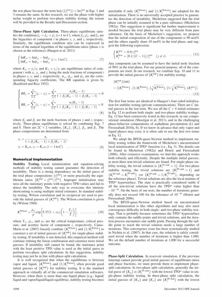
Fig. 2—The phase envelope for CO2 mixing with Oil B at 307.6 Kshowing the single-, two-, and three-phase regions. V, L1, andL2 denote the vapor, CO2-lean, and CO2-rich liquid phases. Thesolid circle represents the bicritical point.
64
66
68
70
72
74
76
78
L1
L1−L
2
V−L1−L
2
V−L1
Pre
ssu
re (
bar
)
CO2 mole fraction
0.65 0.70 0.75 0.80 0.85 0.90 0.95 1.00
Fig. 4—The phase envelope for CO2 mixing with Maljamar sepa-rator oil at 305.35 K showing the single-, two-, and three-phaseregions. V, L1, and L2 denote the vapor, CO2-lean, and CO2-richliquid phases. The solid circle represents the bicritical point.
70
75
80
85
90
95
L1−L
2
V−L1−L
2
V−L1
Pre
ssu
re (
bar
)
CO2 mole fraction
0.65 0.70 0.75 0.80 0.85 0.90 0.95 1.00
Fig. 3—The phase envelope for CO2 mixing with Maljamar reser-voir oil at 305.35 K showing the two- and three-phase regions.V, L1, and L2 denote the vapor, CO2-lean, and CO2-rich liquidphases. The solid circles represent the bicritical points.
1102 December 2012 SPE Journal
1,781 conditions where two-phase stability testing is required.That is because the initial guess of fytrial
i g depends on the testphase despite the fact that the same initial guess of fKstab
i g isused; the iteration may take the wrong path when the phase withlower molar weight is the test phase.
In Table 9, we randomly choose one condition for CO2 mixingwith each hydrocarbon fluid and estimate the CPU time for bothstability testing and phase-split calculation by using our strategy.As before, both single- and two-phase stability testings have simi-
lar CPU time as two-phase split calculation, but three-phase splitcalculation is much more expensive. The computational costincreases with the number of components. In Table 10, we esti-mate the total CPU time used to calculate each phase envelope,including bicritical points. Each phase envelope only needs a fewseconds, although there are many single-, two-, and three-phasestates. Because we require very high accuracy for both equilib-rium ratios and phase fractions, in our strategy the CPU timeincreases close to the critical point.
Because the equal fugacity condition is necessary but not suffi-cient for phase equilibrium, an improper initial guess may
0.1 0.2 0.3 0.4 0.5 0.6 0.7 0.8 0.90
40
80
120
160
200
240
280
L2
V−L1−L2
L1−L
2
L1
V−L1
Pre
ssu
re (
bar
)
CO2 mole fraction
Fig. 5—The phase envelope for impure CO2 (95 mol% CO2 1 5mol% C1) mixing with Bob Slaughter Block oil at 313.71 K show-ing the single-, two-, and three-phase regions. V, L1, and L2
denote the vapor, CO2-lean, and CO2-rich liquid phases. Thesolid circle represents the bicritical point. Note the single-phase L2 appears when the mixture is almost the pure mixinggas.
0.1 0.2 0.3 0.4 0.5 0.6 0.7 0.8 0.9
Pre
ssu
re (
bar
)
CO2 mole fraction
40
80
120
160
200
V−L1−L2
L1
L1−L
2
V−L1
Fig. 6—The phase envelope for impure CO2 (95 mol% CO2 1 5mol% C1) mixing with North Ward Estes oil at 301.48 K showingthe single-, two-, and three-phase regions. V, L1, and L2 denotethe vapor, CO2-lean, and CO2-rich liquid phases. The solidcircles represent the bicritical points.
TABLE 9—CPU TIME OF STABILITY TESTING AND PHASE-SPLIT CALCULATION FOR CO2 MIXING WITH ACID GAS, OIL B,
MALJAMAR RESERVOIR OIL, MALJAMAR SEPARATOR OIL, BOB SLAUGHTER BLOCK OIL, AND NORTH WARD ESTES OIL
AT INDIVIDUAL CONDITIONS
Mixture T (K) P (bar) n (CO2)
CPU Time (sec)
1P-Stab 2P-Split 2P-Stab 3P-Split
Acid gas 178.8 20 0.5 8.89e–4 2.13e–4 1.08e–3 3.50e–3
Oil B 307.6 76 0.9 4.14e–3 3.97e–3 6.43e–3 2.02e–2
North Ward Estes oil 301.48 79 0.80866 6.73e–4 1.18e–3 1.03e3 4.56e–3
TABLE 10—CPU TIME TO CALCULATE PHASE ENVELOPES AND BICRITICAL POINTS FOR
CO2 MIXING WITH ACID GAS, OIL B, MALJAMAR RESERVOIR OIL, MALJAMAR SEPARATOR
OIL, BOB SLAUGHTER BLOCK OIL, AND NORTH WARD ESTES OIL
Mixture
Number of States CPU time (sec)
1P 2P 3P Phase Envelope Bicritical Point
Acid gas 166 249 221 1.68
Oil B 39 133 54 5.02 0.42
Maljamar reservoir oil 0 133 52 6.81 5.01
Maljamar separator oil 65 173 46 0.81 0.09
Bob Slaughter Block oil 224 320 30 0.51 0.08
North Ward Estes oil 119 332 38 1.81 0.61
December 2012 SPE Journal 1103
produce an incorrect phase-split solution with a local minimum ofGibbs free energy. Reliable stability testing can effectively avoidthe blind selection of the initial guess for phase-split calculation.Very often, fK1P-stab
i g with the lowest TPD* value is the best ini-tial guess for two-phase split calculation. However, in a few cases,that may lead to an incorrect two-phase solution. The incorrect so-lution could be either VL or LL type. It is “unstable,” but three-phase solution does not exist. The correct two-phase solution canbe obtained by trying another initial guess [e.g., fK2P-stab
i g withthe lowest TPD* value in two-phase stability testing after theincorrect two-phase split calculation]. The correct solution is sta-ble, and three-phase split calculation is not required. The correctsolution has a Gibbs free energy only slightly lower than theincorrect one. The same observation has been made in Ref.20
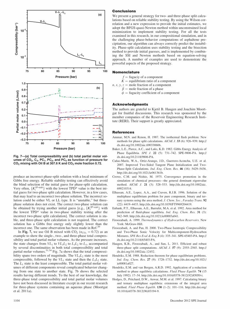
In Fig. 7, we use Oil B mixed with CO2 (nCO2¼ 0:72) as an
example to show the single-, two-, and three-phase total compres-sibility and total partial molar volumes. As the pressure increases,the state changes from VL1 to VL1L2 to L1L2 to L1, accompaniedby several discontinuities in both total compressibility and totalpartial molar volumes.31,34 Fig. 7a shows that the total compressi-bility spans two orders of magnitude. The VL1L2 state is the mostcompressible, followed by the VL1 state and then the L1L2 state.The L1 state is the least compressible. The total partial molar vol-umes of different components reveal complicated behavior chang-ing from one state to another state. Fig. 7b shows the selectedresults having different trends. To the best of our knowledge, thethree-phase total compressibility and total partial molar volumeshave not been discussed in literature except in our recent researchfor three-phase systems containing an aqueous phase (Moortgatet al. 2011a).
Conclusions
We present a general strategy for two- and three-phase split calcu-lations based on reliable stability testing. By using the Wilson cor-relation and a new expression to provide the initial estimates, weadopt the BFGS-quasi-Newton method within unconstrained localminimization to implement stability testing. For all the testsexamined in this research, in our compositional simulation, and inthe challenging phase-behavior computations of asphaltene pre-cipitation, our algorithm can always correctly predict the instabil-ity. Phase-split calculation uses stability testing and the bisectionmethod to provide initial guesses, and is implemented by combin-ing the SSI and Newton methods based on equation-solvingapproach. A number of examples are used to demonstrate thepowerful aspects of the proposed strategy.
Nomenclature
f ¼ fugaciy of a componentK ¼ equilibrium ratio of a component
n, x, y, z ¼ mole fraction of a componentb ¼ mole fraction of a phase/ ¼ fugacity coefficient of a component
Acknowledgments
The authors are grateful to Kjetil B. Haugen and Joachim Moort-gat for fruitful discussions. This research was sponsored by themember companies of the Reservoir Engineering Research Insti-tute (RERI). Their support is greatly appreciated.
References
Ammar, M.N. and Renon, H. 1987. The isothermal flash problem: New
methods for phase split calculations. AIChE J. 33 (6): 926–939. http://
dx.doi.org/10.1002/aic.690330606.
Baker, L.E., Pierce, A.C., and Luks, K.D. 1982. Gibbs Energy Analysis of
Phase Equilibria. SPE J. 22 (5): 731–742. SPE-9806-PA. http://
dx.doi.org/10.2118/9806-PA.
Canas-Marın, W.A., Ortiz-Arango, J.D., Guerrero-Aconcha, U.E. et al.
2007. Improved Two-Sided Tangent Plane Initialization and Two-
Fig. 7—(a) Total compressibility and (b) total partial molar vol-umes of CO2, C3, PC1, PC2, and PC5 as function of pressure forCO2 mixing with Oil B at 307.6 K and CO2 mole fraction 0.72.
1104 December 2012 SPE Journal
Hoteit, H. and Firoozabadi, A. 2006. Simple phase stability-testing algo-
rithm in the reduction method. AIChE J. 52 (8): 2909–2920. http://
dx.doi.org/10.1002/aic.10908.
Hoteit, H. and Firoozabadi, A. 2009. Numerical Modeling of Diffusion in
Fractured Media for Gas-Injection and -Recycling Schemes. SPE J. 14
Whitson, C.H. and Michelsen, M.L. 1989. The negative flash. Fluid PhaseEquilib. 53 (December 1989): 51–71. http://dx.doi.org/10.1016/0378-
3812(89)80072-x.
Wilson, G.M. 1968. A Modified Redlich-Kwong Equation of State, Appli-
cation to General Physical Data Calculations. Presented at the 65th
National AIChE Meeting, Cleveland, Ohio, USA, 4–7 May. Paper 15-
C.
Zhu, Y. 2000. High pressure phase equilibrium through the simulated
annealing algorithm: Application to SRK and PR equations of state.
Presented at the AIChE Annual Meeting, Los Angeles, California,
USA, 12–17 November.
Appendix A—Total Compressibility and TotalPartial Molar Volumes in Single-, Two-,and Three-Phase States
For an individual phase a; fna;kg is the number of moles for com-
ponents, Na ¼X
k
na;k is the total number of moles, vEOSa ¼
ZaRT=p is the molar volume without volume shift, Za is the com-pressibility factor, and ffa;kg is the fugacity for components. For
the whole system, fnk ¼X
a
na;kg is the number of moles for
components, N ¼X
k
nk ¼Xa;k
na;k is the total number of moles,
VEOS ¼X
a
VEOSa ¼
Xa
ZaNaRT=p is the total volume without
volume shift, and V ¼X
a
Va ¼X
a
ðZaNaRT=pþX
k
na;kckÞ is
the total volume with volume shift fckg: In the following expres-sions, the subscripts n ¼ fnkg; n 6¼k ¼ fn1; :::; nk�1; nkþ1; :::; nCg;na ¼ fna;kg; and na;6¼k ¼ fna;1; :::; na;k�1; na;kþ1; :::; na;Cg:
Single-Phase State. When the mixture is in single-phase state,the compressibility and partial molar volumes are given by
jT ¼VEOS
V
1
p� 1
Z
@Z
@p
� �T;n
" #ðA-1Þ
vi ¼NRT
p
@Z
@ni
� �T;p;n6¼i
þ vEOS þ ci ði ¼ 1 to CÞ: ðA-2Þ
Two-Phase State. When the mixture is in two-phase state, thetotal compressibility and total partial molar volumes are given by
jT ¼VEOS
Vp� 1
V
X2
a¼1
(NaRT
p
@Za
@p
� �T;na
þXC
k¼1
NaRT
p
@Za
@na;k
� �T;p;na;6¼k
þ vEOSa þ ck
264
375 @na;k
@p
� �T;n
)� � � ðA-3Þ
vi ¼X2
a¼1
XC
k¼1
NaRT
p
@Za
@na;k
� �T;p;na; 6¼k
þ vEOSa þ ck
264
375 @na;k
@ni
� �T;p;n6¼i
ði¼ 1 to CÞ
� � � � � � � � � � � � � � � � � � � ðA-4Þ
The unknowns in Eqs. A-3 and A-4 can be solved from
XC
k¼1
@f1;j
@n1;k
� �T;p;n1; 6¼k
þ @f2;j
@n2;k
� �T;p;n2; 6¼k
" #@n2;k
@p
� �T;n
¼ @f1;j
@p
� �T;n1
� @f2;j
@p
� �T;n2
ð j ¼ 1 to CÞ � � � � � � � ðA-5Þ
XC
k¼1
@f1;j
@n1;k
� �T;p;n1; 6¼k
þ @f2;j
@n2;k
� �T;p;n2; 6¼k
" #@n2;k
@ni
� �T;p;n6¼i
¼XC
k¼1
dki@f1;j
@n1;k
� �T;p;n1;6¼k
ð j ¼ 1 to CÞ � � � � � � � � � � ðA-6Þ
combined with the mass balance fnk ¼X2
a¼1
na;kg: dki is the Kro-
necker delta function. Note jT ¼ 1 for C ¼ 1.
Three-Phase State. When the mixture is in three-phase state, thetotal compressibility and total partial molar volumes are given by
jT ¼VEOS
Vp� 1
V
X3
a¼1
(NaRT
p
@Za
@p
� �T;na
þXC
k¼1
NaRT
p
@Za
@na;k
� �T;p;na;6¼k
þ vEOSa þ ck
264
375 @na;k
@p
� �T;n
)
� � � � � � � � � � � � � � � � � � � ðA-7Þ
vi ¼X3
a¼1
XC
k¼1
NaRT
p
@Za
@na;k
� �T;p;na; 6¼k
þ vEOSa þ ck
264
375 @na;k
@ni
� �T;p;n6¼i
ði¼ 1 to CÞ
� � � � � � � � � � � � � � � � � � � ðA-8Þ
. . . . . . . . . . . . . . . . .
. . . . .
1106 December 2012 SPE Journal
The unknowns in Eqs. A-7 and A-8 can be solved from
XC
k¼1
@f1;j@n1;k
� �T;p;n1;6¼k
þ @f2;j@n2;k
� �T;p;n2;6¼k
26664
37775
@n2;k
@p
� �T;n
þ @f1;j@n1;k
� �T;p;n1;6¼k
@n3;k
@p
� �T;n
¼ @f1;j@p
� �T;n1
� @f2;j@p
� �T;n2
8>>><>>>:
9>>>=>>>;
XC
k¼1
@f1;j@n1;k
� �T;p;n1;6¼k
@n2;k
@p
� �T;n
þ
@f1;j@n1;k
� �T;p;n1;6¼k
þ @f3;j@n3;k
� �T;p;n3;6¼k
26664
37775 @n3;k
@p
� �T;n
¼ @f1;j@p
� �T;n1
� @f3;j@p
� �T;n3
8>>>>>>>>><>>>>>>>>>:
9>>>>>>>>>=>>>>>>>>>;
ð j ¼ 1 to CÞ
8>>>>>>>>>>>>>>>>>>><>>>>>>>>>>>>>>>>>>>:
� � � � � � � � � � � � � � � � � � � ðA-9Þ
XC
k¼1
@f1;j@n1;k
� �T;p;n1;6¼k
þ @f2;j@n2;k
� �T;p;n2;6¼k
26664
37775
@n2;k
@ni
� �T;p;n6¼i
þ @f1;j
@n1;k
� �T;p;n1; 6¼k
@n3;k
@ni
� �T;p;n 6¼i
¼XC
k¼1
dki@f1;j@n1;k
� �T;p;n1; 6¼k
8>>>><>>>>:
9>>>>=>>>>;
XC
k¼1
@f1;j@n1;k
� �T;p;n1; 6¼k
@n2;k
@ni
� �T;p;n 6¼i
þ
@f1;j
@n1;k
� �T;p;n1; 6¼k
þ @f3;j
@n3;k
� �T;p;n3;6¼k
26664
37775 @n3;k
@ni
� �T;p;n 6¼i
¼XC
k¼1
dki@f1;j
@n1;k
� �T;p;n1; 6¼k
8>>>>>>>>><>>>>>>>>>:
9>>>>>>>>>=>>>>>>>>>;
ðj ¼ 1 to CÞ
8>>>>>>>>>>>>>>>>>>>><>>>>>>>>>>>>>>>>>>>>:
� � � � � � � � � � � � � � � � � � � ðA-10Þ
combined with the mass balance fnk ¼X3
a¼1
na;kg: A special case
of three-phase total compressibility and total partial molar vol-umes for the system containing water and two hydrocarbon phaseshas been recently presented in Ref. 53.
Zhidong Li is a postdoctoral researcher at RERI. email: [email protected]. His research interest is in thermodynamics of IOR/EOR withgas/water injection, asphaltene precipitation and stabiliza-tion, shale gas/oil, multiphase equilibrium computation, andPVT modeling. Li holds BS and MS degrees from Tsinghua Uni-versity, Beijing, China, and a PhD degree from the University ofCalifornia at Riverside, all in chemical engineering.
Abbas Firoozabadi is the senior scientist and director at RERI.He also teaches at Yale University. email: [email protected]. Hismain research activities center on thermodynamics of hydro-carbon reservoirs and production and on multiphase-multi-component flow in fractured petroleum reservoirs. Firoozabadiholds a BS degree from the Abadan Institute of Technology,Abadan, Iran, and MS and PhD degrees from the Illinois Insti-tute of Technology, Chicago, all in gas engineering. Firooza-badi is the recipient of the 2002 SPE/AIME Anthony Lucas GoldMedal and the 2004 SPE John Franklin Carll Award. Firooza-badi is also the recipient of the 2009 SPE Honorary MembershipAward. Firoozabadi has become a member of the NationalAcademy of Engineering since 2011.