Generalised Wasserstein Dice Score for Imbalanced Multi-class Segmentation using Holistic Convolutional Networks Lucas Fidon 1 , Wenqi Li 1 , Luis C. Garcia-Peraza-Herrera 1 , Jinendra Ekanayake 2,3 , Neil Kitchen 2 , S´ ebastien Ourselin 1,3 , and Tom Vercauteren 1,3 1 TIG, CMIC, University College London, London, UK 2 NHNN, University College London Hospitals, London UK 3 Wellcome / EPSRC Centre for Interventional and Surgical Sciences, UCL, London, UK Abstract. The Dice score is widely used for binary segmentation due to its robustness to class imbalance. Soft generalisations of the Dice score allow it to be used as a loss function for training convolutional neural networks (CNN). Although CNNs trained using mean-class Dice score achieve state-of-the-art results on multi-class segmentation, this loss function does neither take advantage of inter-class relationships nor multi-scale information. We argue that an improved loss function should balance misclassifications to favour predictions that are semanti- cally meaningful. This paper investigates these issues in the context of multi-class brain tumour segmentation. Our contribution is threefold. 1) We propose a semantically-informed generalisation of the Dice score for multi-class segmentation based on the Wasserstein distance on the prob- abilistic label space. 2) We propose a holistic CNN that embeds spatial information at multiple scales with deep supervision. 3) We show that the joint use of holistic CNNs and generalised Wasserstein Dice score achieves segmentations that are more semantically meaningful for brain tumour segmentation. 1 Introduction Automatic brain tumour segmentation is an active research area. Learning-based methods using convolutional neural networks (CNNs) have recently emerged as the state of the art [9,11]. One of the challenges is the severe class imbalance. Two complementary ways have traditionally been used when training CNNs to tackle imbalance: 1) using a sampling strategy that imposes constraints on the selection of image patches; and 2) using pixel-wise weighting to balance the con- tribution of each class in the objective function. For CNN-based segmentation, samples should ideally be entire subject volumes to support the use of fully convolutional network and maximise the computational efficiency of convolu- tion operations within GPUs. As a result, weighted loss functions appear more promising to improve CNN-based automatic brain tumour segmentation. Using arXiv:1707.00478v4 [cs.CV] 29 Aug 2017
Lucas Fidon1, Wenqi Li1, Luis C. Garcia-Peraza-Herrera1,Jinendra Ekanayake2,3, Neil Kitchen2,
Sebastien Ourselin1,3, and Tom Vercauteren1,3
1 TIG, CMIC, University College London, London, UK2 NHNN, University College London Hospitals, London UK
3 Wellcome / EPSRC Centre for Interventional and Surgical Sciences,UCL, London, UK
Abstract. The Dice score is widely used for binary segmentation dueto its robustness to class imbalance. Soft generalisations of the Dicescore allow it to be used as a loss function for training convolutionalneural networks (CNN). Although CNNs trained using mean-class Dicescore achieve state-of-the-art results on multi-class segmentation, thisloss function does neither take advantage of inter-class relationshipsnor multi-scale information. We argue that an improved loss functionshould balance misclassifications to favour predictions that are semanti-cally meaningful. This paper investigates these issues in the context ofmulti-class brain tumour segmentation. Our contribution is threefold. 1)We propose a semantically-informed generalisation of the Dice score formulti-class segmentation based on the Wasserstein distance on the prob-abilistic label space. 2) We propose a holistic CNN that embeds spatialinformation at multiple scales with deep supervision. 3) We show thatthe joint use of holistic CNNs and generalised Wasserstein Dice scoreachieves segmentations that are more semantically meaningful for braintumour segmentation.
1 Introduction
Automatic brain tumour segmentation is an active research area. Learning-basedmethods using convolutional neural networks (CNNs) have recently emerged asthe state of the art [9,11]. One of the challenges is the severe class imbalance.Two complementary ways have traditionally been used when training CNNs totackle imbalance: 1) using a sampling strategy that imposes constraints on theselection of image patches; and 2) using pixel-wise weighting to balance the con-tribution of each class in the objective function. For CNN-based segmentation,samples should ideally be entire subject volumes to support the use of fullyconvolutional network and maximise the computational efficiency of convolu-tion operations within GPUs. As a result, weighted loss functions appear morepromising to improve CNN-based automatic brain tumour segmentation. Using
arX
iv:1
707.
0047
8v4
[cs
.CV
] 2
9 A
ug 2
017
2 Lucas Fidon et al.
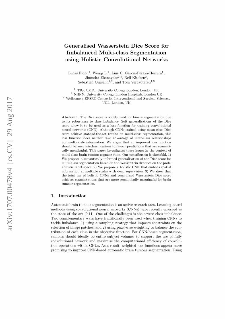
Tumour
Tumour core Edema(2)
Enhancing core(4)
Non-enhancing tumour
Necrotic core(1)
Non-enhancing core(3)
0,2
0,2
0,1
0,1
0,10,1
Fig. 1. Left: tree on BraTS label space. Edge weights have been manually selected toreflect the distance between labels. Right: illustration on a T2 scan from BraTS’15 [14].
soft generalisations of the Dice score (a popular overlap measure for binary seg-mentation) directly as a loss function has recently been proposed [15,18]. Byintroducing global spatial information into the loss function, the Dice loss hasbeen shown to be more robust to class imbalance. However at least two sourcesof information are not fully utilised in this formulation: 1) the structure of thelabel space; and 2) the spatial information across scales. Considering the classimbalance and the hierarchical label structure illustrated in Fig.1, both of themare likely to play an important role for multi-class brain tumour segmentation.
In this paper, we propose two complementary contributions that leverageprior knowledge about brain tumour structure. First, we exploit the Wasser-stein distance [7,17], which can naturally embed semantic relationships betweenclasses for the comparison of label probability vectors, to generalise the Dicescore for multi-class segmentation. Second, we propose a new holistic CNN ar-chitecture inspired by [8,19] that embeds spatial information at different scalesand introduces deep supervision during the CNN training. We show that thecombination of the proposed generalised Wasserstein Dice score and our Holis-tic CNN achieves better generalisation compared to both mean soft Dice scoretraining and classic CNN architectures for multi-class brain tumour segmenta-tion.
2 A Wasserstein approach for multi-class soft Dice score
2.1 Dice score for crisp binary segmentation
The Dice score is a widely used overlap measure for pairwise comparison of binarysegmentations S and G. It can be expressed both in terms of set operations orstatistical measures as:
D =2|S ∩G||S|+ |G|
=2ΘTP
2ΘTP +ΘFP +ΘFN=
2ΘTP
2ΘTP +ΘAE(1)
with ΘTP the number of true positives, ΘFP /ΘFN the number of false posi-tives/false negatives, and ΘAE = ΘFP +ΘFN the number of all errors.
Generalised Wasserstein Dice Score 3
2.2 Dice score for soft binary segmentation
Extensions to soft binary segmentations [1,2] rely on the concept of disagreementfor pairs of probabilistic classifications. The classes Si and Gi of each voxeli ∈ X can be defined as random variables on the label space L = {0, 1} andthe probabilistic segmentations can be represented as label probability maps:p = {pi := P (Si = 1)}i∈X and g = {gi := P (Gi = 1)}i∈X. We denote P (L) theset of label probability vectors. We can now generalise ΘTP and ΘAE to softsegmentations:
ΘAE =∑i∈X
|pi − gi|, ΘTP =∑i∈X
gi(1− |pi − gi|) (2)
In the common case of a crisp segmentation g (i.e. ∀i ∈ X, gi ∈ {0, 1}), theassociated soft Dice score can be expressed as:
D(p, g) =2∑
i gipi∑
i(gi + pi)
(3)
A second variant has been used in [15], with a quadratic term in the denominator.
2.3 Previous work on multi-class Dice score
The easiest way to derive a unique criterion from the soft binary Dice score formulti-class segmentation is to consider the mean Dice score:
Dmean(p, g) =1
|L|∑l∈L
2∑
i gilp
il∑
i(gil + pil)
(4)
where {gil}i∈X, l∈L, {pil}i∈X, l∈L are the set label probability vectors for all voxelsfor the ground truth and the prediction.
A generalised soft multi-class Dice score has also been proposed in [4,18] bygeneralising the set theory definition of the Dice score (1):
DFM (p, g) =2∑
l αl
∑i min(pil, g
il)∑
l αl
∑i(p
il + gil)
(5)
where {αl}l∈L allows to weight the contribution of each class. However, thosedefinitions are still based only on pairwise comparisons of probabilities associatedwith the same label and don’t take into account inter-class relationships.
2.4 Wasserstein distance between label probability vectors
The Wasserstein distance (also sometimes called the Earth Mover’s Distance)represents the minimal cost to transform a probability vector p into another oneq when for all l, l′ ∈ L, the cost to move a unit from l to l′ is defined as thedistance Ml,l′ between l and l′. This is a way to map a distance matrix M (often
4 Lucas Fidon et al.
referred to as the ground distance matrix ) on L, into a distance on P (L) thatleverages prior knowledges about L. In the case of a finite set L, for p, q ∈ P (L),the Wasserstein distance between p and q derived from M can be defined as thesolution of a linear programming problem [17]:
WM (p, q) = minTl,l′
∑l,l′∈L
Tl,l′Ml,l′ ,
subject to ∀l ∈ L,∑l′∈L
Tl,l′ = pl, and ∀l′ ∈ L,∑l∈L
Tl,l′ = ql′ .(6)
where T = (Tl,l′)l,l′∈L is a joint probability distribution for (p, q) with marginal
distributions p and q. A value T that minimises (6) is called an optimal transportbetween p and q for the distance matrix M .
2.5 Soft multi-class Wasserstein Dice score
The Wasserstein distance WM in (6) yields a natural way to compare two labelprobability vectors in a semantically meaningful manner by supplying a distancematrix M on L. Hence we propose using it to generalise the measure of dis-agreement between a pair of label probability vectors and provide the followinggeneralisations:
ΘAE =∑i∈X
WM (pi, gi) (7)
ΘlTP =
∑i∈X
gil(WM (l, b)−WM (pi, gi)), ∀l ∈ L \ {b} (8)
where WM (l, b) is shorthand for Ml,b and M is chosen such that the backgroundclass b is always the furthest away from the other classes. To generalise ΘTP , wepropose to weight the contribution of the classes similarly to (5):
ΘTP =∑l∈L
αlΘlTP (9)
We chose αl = WM (l, b) to make sure that background voxels do not contributeto ΘTP . The Wasserstein Dice score with respect to M can then be defined as:
DM (p, g) =2∑
lWM (l, b)
∑i g
il(W
M (l, b)−WM (pi, gi))
2∑
l[WM (l, b)
∑i g
il(W
M (l, b)−WM (pi, gi))] +∑
iWM (pi, gi)
(10)In the binary case, setting M = [ 0 1
1 0 ] leads to WM (pi, gi) = |pi−gi| and reducesthe proposed Wasserstein Dice score to the soft binary Dice score (2).
2.6 Wasserstein Dice loss with crisp ground truth
Previous work on Wasserstein distance-based loss functions for deep learninghave been limited because of the computational burden [17]. However, in the
Generalised Wasserstein Dice Score 5
case of a crisp ground-truth {gi}i, and for any prediction {pi}i, a closed-formsolution exists for (6). An optimal transport is ∀l, l′ ∈ L, Tl,l′ = pilg
il′ and the
Wasserstein distance becomes:
WM (pi, gi) =∑l,l′∈L
Ml,l′pilg
il′ (11)
We define the Wasserstein Dice loss derived from M as LDM := 1−DM .
3 Holistic convolutional networks for multi-scale fusion
We now describe a holistically-nested convolutional neural network (HCNN) forimbalanced multi-class brain tumour segmentation inspired by the holistically-nested edge detection (HED) introduced in [19]. HCNN has been used success-fully for some imbalanced learning tasks such as edge detection in natural im-ages [19] and surgical tool segmentation [8]. The HCNN features multi-scaleprediction and intermediate supervision. It can produce a unified output usinga fusion layer while implicitly embedding spatial information in the loss. Wefurther improve on the ability of HCNNs to deal with imbalanced datasets byleveraging the proposed generalised Wasserstein Dice loss. To keep up with state-of-the-art CNNs, we also employ ELU as activation function [3] and use residualconnections [10]. Residual blocks include a pair of 33 convolutional filters andBatch Normalisation [20]. The proposed architecture is illustrated in Fig.2.
3.1 Multi-scale prediction to leverage spatial consistency in the loss
As the receptive field increases across successive layers, predictions computed atdifferent layers embed spatial information at different scales. Especially for im-balanced multi-class segmentation, different scales can contain complementary
1x1x1 Conv.
+
70
+
70
70
+
70
70
70
+
70
70
+
70
70
70
+
70
+ +
70
70
+
70
70
70
+
70
70
+
70
70
70
+
70
70
70
Loss Loss
70
Softmax
2x2
Loss
70
70
Softmax
2x2
Loss
70
SoftmaxSoftmax
Softmax
Loss
BN + ELU + 3x3x3 Conv.
BN + ELU + 3x3x3 Dilated Conv. (Factor 2)
Max. Pooling
Deconvolution
Scale 1 Scale 2 Scale 3 Scale 4
Fused scale
2x2
Fig. 2. Proposed holistically-nested CNN for multi-class labelling of brain tumours.
6 Lucas Fidon et al.
information. In this paper, to increase the receptive field and avoid redundancybetween successive scale predictions, max pooling and dilated convolutions (witha factor of 2 similar to [13]) have been used. As predictions are computed regu-larly at intermediate scales along the network (Fig.2), we chose to increase thenumber of features before the first prediction is made. For simplicity reasons,we then selected the same value for all hidden layers (fixed to 70 given memoryconstraints).
3.2 Multi-scale fusion and deep supervision for multi-classsegmentation
While classic CNNs provide only one output, HCNNs provide outputs ys at Sdifferent layers of the network, and combine them to provide a final output yfuse:
(yfusel )l∈L = Softmax(( S∑
s=1
wl,sysl
)l∈L
).
As different scales can be of different importance for different classes we learnclass-specific fusion weights wl,s. This transformation can also be represented bya convolution layer with kernels of size 13 where the multi-scale predictions arefused in separated branches for each class, as illustrated in Fig. 2 similarly tothe scalable layers introduced in [5]. In addition to applying the loss functionL to the fused prediction, L is also applied to each scale-specific predictionthereby providing deep supervision (coefficients λ and λs are set to 1/(S + 1)for simplicity):
LTotal((ys)Ss=1, y
fuse, y) = λL(yfuse, y) +
S∑s=1
λsL(ys, y)
4 Implementation details
4.1 Brain tumour segmentation
We evaluate our HCNN model and Wasserstein Dice loss functions on the taskof brain tumour segmentation using BraTS’15 training set that provides mul-timodal images (T1, T1c, T2 and Flair) for 220 high-grade gliomas subjectsand 54 low-grade gliomas subjects. We divide it randomly into 80% for train-ing, 10% for validation and 10% for testing so that the proportion of high-gradeand low-grade gliomas subjects is the same in each fold. The scans are labelledwith five classes (Fig. 1): (0) background, (1) necrotic core, (2) edema, (3) non-enhancing core and (4) enhancing tumour. The most common evaluation criteriafor BraTS is to use the Dice scores for the whole tumour (labels 1,2,3,4), the coretumour (labels 1,3,4) and the enhanced tumour (label 4). All the scans of BraTSdataset are skull stripped, resampled to a 1mm isotropic grid and co-registeredto the T1-weighted volume of each patient. Additionally, we applied histogramstandardisation to each imaging modality independently [16].
Generalised Wasserstein Dice Score 7
Table 1. Evaluation of different multi-class Dice scores for training and testing.LDMtree−PT stands for pre-training the HCNN with mean Dice score (4 epochs) andretraining it with LDMtree (85 epochs).
Loss function Evaluation: Mean(std) Dice scores (%)
Whole Core Enh. Mean Dice DM0−1 DMtree
Mean Dice 83(13) 70(21) 68(26) 60(12) 77(11) 80(12)L
We train the networks using ADAM [12] with a learning rate lr = 0.01, β1 =0.9 and β2 = 0.999. To regularise the network, we use early stopping on thevalidation set and dropout in all residual blocks before the last activation (asproposed in [20]), with a probability of 0.6. We use multi-modal volumes ofsize 803 from one subject concatenated as input during training and a samplingstrategy to maximise the number of classes in each patch. Experiments have beenperformed using Tensorflow 1.1 4 and a Nvidia GeForce GTX Titan X GPU.
5 Results
We evaluate the usefulness of the proposed soft multi-class Wasserstein Diceloss and the proposed HCNN with deep supervision. We compare the soft multi-class Wasserstein Dice loss to the state-of-the-art mean Dice score [5,13] for thetraining of our HCNN in Table 1 and 2. We also evaluate the segmentation atthe different scales of the HCNN in Table 3.
5.1 Examples of distance metrics on BraTS label space
To illustrate the flexibility of the proposed generalised Wasserstein Dice score,we evaluate two semantically driven choices for the distance matrix M on L:
M0−1 is associated with the discrete distance on L with no inter-class relation-ship. Mtree is derived from the tree structure of L illustrated in Fig. 1. Thistree is based on the tumour hierarchical structure: whole, core and enhancingtumour. We set branch weights to 0.1 for contiguous nodes and 0.2 otherwise.
4 The code is publicly available as part of NiftyNet (http://niftynet.io)
Fig. 3. Qualitative comparison of HCNN predictions at testing after training with theproposed Generalised Wasserstein Dice loss (LDMtree−PT ) or mean-class Dice loss.Training with LDMtree−PT allows avoiding implausible misclassifications encounteredin predictions after training with mean-class Dice loss (emphasized by white arrows).
5.2 Evaluation and training with multi-class Dice score
The mean Dice corresponds to the mean of soft Dice scores for each class asused in [5,13]. Results in Table 1 confirm that training with mean Dice score,DM0−1 or DMtree allow maximising results for the associated multi-class Dicescore during inference.
While DMtree takes advantage of prior information about the hierarchicalstructure of the tumour classes it makes the optimisation more complex byadding more constraints. To relax those constraints, we propose to pretrain thenetwork using the mean Dice score during a few epochs (4 in our experiment)and then retrain it using DMtree . This approach leads to the best results for allcriteria, as illustrated in the last line of Table 1. Moreover, it produces segmenta-tions that are more semantically plausible compared to the HCNN trained withmean Dice only as illustrated by Fig. 3.
5.3 Impact of the Wasserstein Dice loss on class confusion
Evaluating brain tumour segmentation using Dice scores of label subsets likewhole, core and enhancing tumour doesn’t allow measuring the ability of a modelto learn inter-class relationships and to favour voxel classifications, be it corrector not, that are semantically as close as possible to the ground truth. We proposeto measure class confusion using pairwise comparisons of all labels pair betweenthe predicted segmentation and the ground truth (Table 2). Mathematically, forall l, l′ ∈ L, the quantity in row l and colomn l′ stands for the soft binary Dicescore:
Dl,l′ =2∑
i gilp
il′∑
i(gil + pil′)
(12)
Generalised Wasserstein Dice Score 9
Table 2. Dice score evaluation of the confusion after training the HCNN using differentloss functions. Each line (resp. column) corresponds to the mean(standard deviation)Dice scores (%) of a region of the ground truth (resp. prediction) with all regions ofthe prediction (resp. ground truth) computed on the testing set.
Mean Dice Prediction
Ground truth Background Necrotic core Edema Non-enh. Enh.
Results in Table 2 compare class confusion of the proposed HCNN after beingtrained either using mean Dice loss, tree-based Wasserstein Dice loss (LDMtree ) ortree-based Wasserstein Dice loss pre-trained with mean Dice loss(LDMtree−PT ).The first one aims only at maximising the true positives (diagonal) while thetwo other additionally aim at balancing the misclassifications to produce sem-natically meaningful segmentations.
The network trained with mean Dice loss segments correctly most of the vox-els (diagonal in Table 2) but makes misclassifications that are not semanticallymeaningful. For example, it makes poor differentiation between the edema andthe core tumour as can be seen in the line corresponding to edema in Table 2and in Fig. 3.
In contrast, the network trained with LDMtree makes more meaningful con-fusion but it is not able to differentiate necrotic core and non-enhancing tumourat all (columns 2 and 4). It illustrates the difficulty to train the network withLDMtree starting from a random initialisation because LDMtree embeds moreconstraints than the mean Dice loss.LDMtree−PT allows combining advantages of both loss function: pre-training
the network using the mean Dice loss allows initialising it so that it produces
10 Lucas Fidon et al.
Table 3. Evaluation of scale-specific and fused predictions of the HCNN with Dicescore of whole, core, enhancing tumour and DMtree after being pre-trained with meanDice score (4 epochs) and retrained with LDMtree (85 epochs).
quickly an approximation of the segmentation, and retraining it with LDMtree
allows reaching a model which provides semantically meaningful segmentations(Fig. 3) with a higher rate of true positives compared to training with LDMtree
or mean Dice loss alone (Table 2).
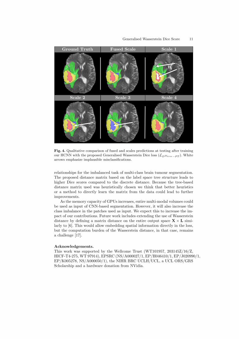
5.4 Evaluation of deep supervision
Results in Table 3 are obtained after pre-training HCNN with mean Dice scoreduring 4 epochs and then training it with LDMtree during 85 additional epochs.Scales 2 to 4 and fused achieve similar Dice scores for whole, core tumour andthe objective function DMtree while scale 1 obtains lower Dice scores. Holes intumour segmentations produced by scale 1, as illustrated in Fig. 4, suggest anunsufficient receptive field could account for those lower Dice scores. The bestresult for the enhancing tumour is achievied by both scale 2 and fused, whichwas expected as this is the smallest region of interest and the full resolution ismaintained until scale 2. Moreover, as illustrated in Fig. 4, scales 3 and 4 fail atsegmenting the thinest regions of the tumour because of their lower resolutioncontrary to scales 1 and 2 and fused. However, scales 1 to 3 contained implausi-ble segmentation regions contrary to scale 4 and fused. This suggests trade-offsbetween high receptive field and high resolution that are class specific. It con-firms the usefulness of the multi-scale holistic approach for the multi-class braintumour segmentation task.
6 Conclusion and future work
We proposed a semantically driven generalisation of the Dice score for soft multi-class segmentation based on the Wasserstein distance. This embeds prior knowl-edge about inter-class relationships represented by a distance matrix on the labelspace. Additionally, we proposed a holistic convolutional network that uses multi-scale predictions and deep supervision to make use of multi-scale information.We successfully used the proposed Wasserstein Dice score as a loss function totrain our holistic networks and show the importance of multi-scale and inter-class
Generalised Wasserstein Dice Score 11
Ground Truth Fused Scale Scale 1
Scale 2 Scale 3 Scale 4
Fig. 4. Qualitative comparison of fused and scales predictions at testing after trainingour HCNN with the proposed Generalised Wasserstein Dice loss (LDMtree−PT ). Whitearrows emphasize implausible misclassifications.
relationships for the imbalanced task of multi-class brain tumour segmentation.The proposed distance matrix based on the label space tree structure leads tohigher Dice scores compared to the discrete distance. Because the tree-baseddistance matrix used was heuristically chosen we think that better heuristicsor a method to directly learn the matrix from the data could lead to furtherimprovements.
As the memory capacity of GPUs increases, entire multi-modal volumes couldbe used as input of CNN-based segmentation. However, it will also increase theclass imbalance in the patches used as input. We expect this to increase the im-pact of our contributions. Future work includes extending the use of Wassersteindistance by defining a matrix distance on the entire output space X × L simi-larly to [6]. This would allow embedding spatial information directly in the loss,but the computation burden of the Wasserstein distance, in that case, remainsa challenge [17].
Acknowledgements.This work was supported by the Wellcome Trust (WT101957, 203145Z/16/Z,HICF-T4-275, WT 97914), EPSRC (NS/A000027/1, EP/H046410/1, EP/J020990/1,EP/K005278, NS/A000050/1), the NIHR BRC UCLH/UCL, a UCL ORS/GRSScholarship and a hardware donation from NVidia.
12 Lucas Fidon et al.
References
1. Anbeek, P., Vincken, K.L., van Bochove, G.S., van Osch, M.J., van der Grond, J.:Probabilistic segmentation of brain tissue in MR imaging. NeuroImage 27(4), 795– 804 (2005)
3. Clevert, D.A., Unterthiner, T., Hochreiter, S.: Fast and accurate deep networklearning by exponential linear units (elus). arXiv:1511.07289 (2015)
4. Crum, W.R., Camara, O., Hill, D.L.: Generalized overlap measures for evaluationand validation in medical image analysis. IEEE TMI 25(11), 1451–1461 (2006)
5. Fidon, L., Li, W., Garcia-Peraza-Herrera, L.C., Ekanayake, J., Kitchen, N.,Ourselin, S., Vercauteren, T.: Scalable multimodal convolutional networks for braintumour segmentation. MICCAI (2017)
6. Fitschen, J.H., Laus, F., Schmitzer, B.: Optimal transport for manifold-valuedimages. In: International Conference on Scale Space and Variational Methods inComputer Vision. pp. 460–472. Springer (2017)
7. Frogner, C., Zhang, C., Mobahi, H., Araya, M., Poggio, T.A.: Learning with awasserstein loss. In: NIPS. pp. 2053–2061 (2015)
8. Garcia-Peraza-Herrera, L.C., Li, W., Fidon, L., Gruijthuijsen, C., Devreker, A.,Attilakos, G., Deprest, J., Vander Poorten, E., Stoyanov, D., Vercauteren, T.,Ourselin, S.: ToolNet : Holistically-Nested Real-Time Segmentation of RoboticSurgical Tools. In: IROS (2017)
9. Havaei, M., Davy, A., Warde-Farley, D., Biard, A., Courville, A., Bengio, Y., Pal,C., Jodoin, P.M., Larochelle, H.: Brain tumor segmentation with deep neural net-works. Med. Image Anal. 35, 18–31 (2017)
10. He, K., Zhang, X., Ren, S., Sun, J.: Deep residual learning for image recognition.In: IEEE CVPR (2016)
11. Kamnitsas, K., Ledig, C., Newcombe, V.F., Simpson, J.P., Kane, A.D., Menon,D.K., Rueckert, D., Glocker, B.: Efficient multi-scale 3D CNN with fully connectedCRF for accurate brain lesion segmentation. Med. Image Anal. 36, 61–78 (2017)
12. Kingma, D., Ba, J.: Adam: A method for stochastic optimization. arXiv:1412.6980(2014)
13. Li, W., Wang, G., Fidon, L., Ourselin, S., Cardoso, M.J., Vercauteren, T.: On thecompactness, efficiency, and representation of 3D convolutional networks: Brainparcellation as a pretext task. IPMI (2017)
14. Menze, B.H., Jakab, A., Bauer, S., Kalpathy-Cramer, J., Farahani, K., Kirby, J.,Burren, Y., Porz, N., Slotboom, J., Wiest, R., et al.: The multimodal brain tumorimage segmentation benchmark (BraTS). IEEE TMI 34(10), 1993–2024 (2015)
15. Milletari, F., Navab, N., Ahmadi, S.A.: V-Net: Fully convolutional neural networksfor volumetric medical image segmentation. In: Proc. 3DV’16. pp. 565–571 (2016)
16. Nyul, L.G., Udupa, J.K., Zhang, X.: New variants of a method of MRI scale stan-dardization. IEEE TMI 19(2), 143–150 (Feb 2000)
17. Pele, O., Werman, M.: Fast and robust earth mover’s distances. ICCV (2009)18. Sudre, C.H., Li, W., Vercauteren, T., Ourselin, S., Cardoso, M.J.: Generalised
Dice overlap as a deep learning loss function for highly unbalanced segmentations.arXiv:1707.03237 (2017)