Generalized Additive Models (GAMs)

Israel BorokiniAdvanced Analysis Methods in Natural Resources and Environmental Science

(NRES 746)

October 3, 2016

Outline

• Quick refresher on linear regression

• Generalized Additive Models• Statistical expression

• Operations

• Research Applications

• R packages for GAMs

• Examples

• K selection

Regression• Regression methods are used to investigate relationships between

predictors and response variables

• A good model should perform three functions: description, inference and predictions

Linear Regression Model• Bivariate regression: Y = α + βX + ε

• Multivariate regression: Y = α + β1X1 + β2X2 + … + βnXn + ε

• Quadratic regression: Y = α + β1X1 + β2X22 + ε

• Polynomial regression: Y = α + β1X1 + β2X22 + β3X3

3 + βnXnn + ε

• Y - response variable X - explanatory variable

• ε - residual error, to cover unexplained information, assumed to be normally distributed with mean of 0 and δ2

• α and β are intercept and slope respectively, to be determined at CI = 95%

• N – sample size

• OLS regression computes values of α and β that best fit the response by minimizing sum of squared errors (assuming linearity and homoscedasticity)

where ε ~ N (0,δ2)

Assumptions of Linear regression models

• Linearity (sensitive to outliers & data inaccuracy)

• Multivariate normality

• Little or no multicollinearity & singularity

• No auto-correlation

• Homoscedasticity

• Prefers large response variable (20:1)

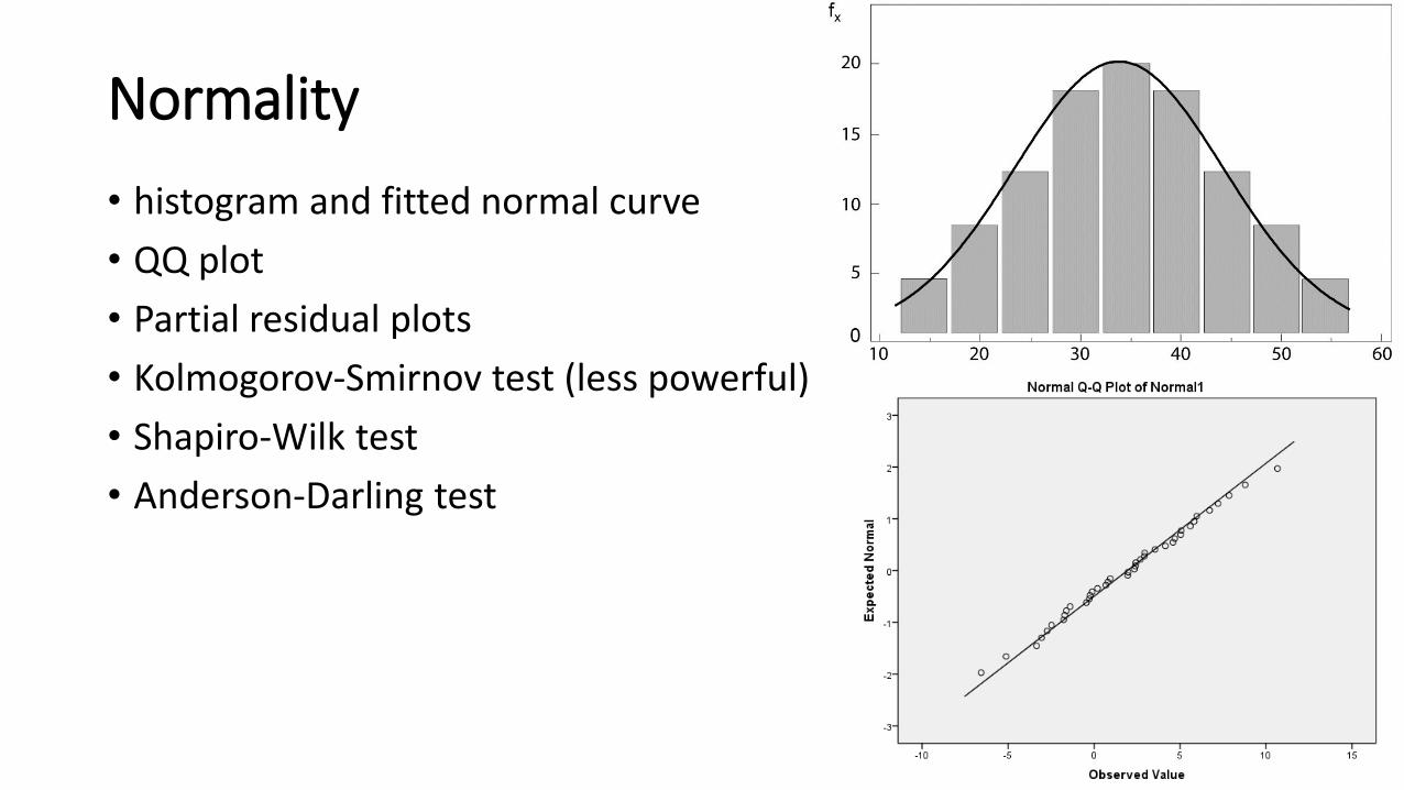
Normality

• histogram and fitted normal curve

• QQ plot

• Partial residual plots

• Kolmogorov-Smirnov test (less powerful)

• Shapiro-Wilk test

• Anderson-Darling test

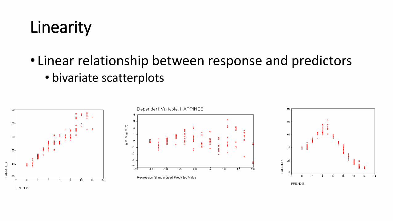
Linearity

• Linear relationship between response and predictors • bivariate scatterplots

Multicollinearity and singularity

• Multicollinearity – strong correlations between (or among) predictors

• Singularity – when predictors are perfectly correlated, that is r = 1.0

• Effects: bias predictions

• Solutions: remove some variables or factor analysis

• Detected with the following tests• Correlation matrix (correlation values >1 indicates multicollinearity)

• Tolerance measures: T = 1 – R2 (T < 0.1 indicates multicollinearity)

• Variance inflation factor: VIF = 1/T (VIF >100 indicates multicollinearity)

• Condition index (values ≥10 indicates multicollinearity)

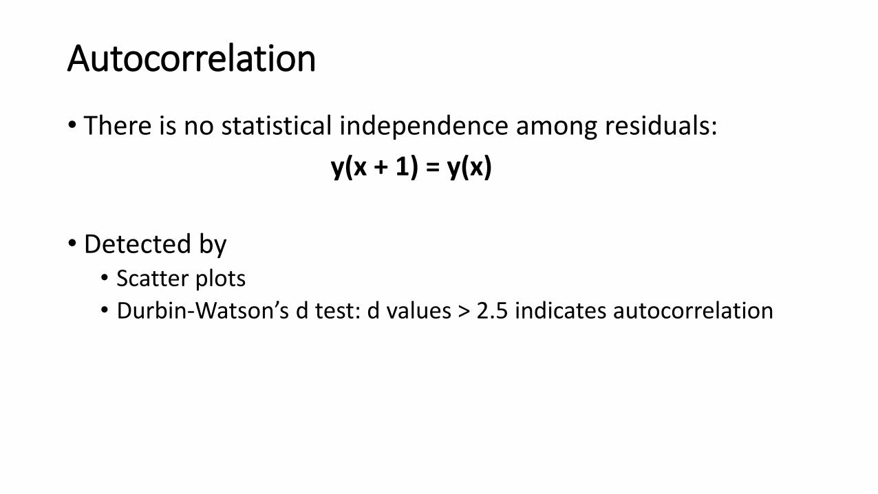
Autocorrelation

• There is no statistical independence among residuals:

y(x + 1) = y(x)

• Detected by• Scatter plots

• Durbin-Watson’s d test: d values > 2.5 indicates autocorrelation

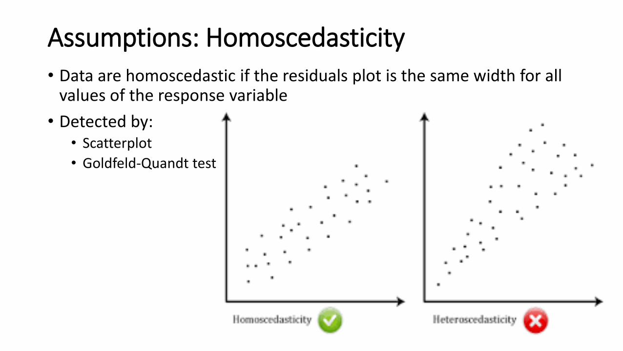
Assumptions: Homoscedasticity• Data are homoscedastic if the residuals plot is the same width for all

values of the response variable

• Detected by: • Scatterplot

• Goldfeld-Quandt test

Transformations

• Moderate deviation: square root transformation

• Substantial non-normal: log transformation

• Severe non-normal: inverse transformation

• Negative skew: data reflection before transformation

• Heteroscedasticity: Use general least squares

• Non-linear: non-linear least squares or MLE

http://rogeriofvieira.com/wp-content/uploads/2016/05/Data-Transformations-1.pdf

Transformation should be considered during model interpretations

Model types

• Parametric: strong parametric assumptions. Average change in response variable is proportional to change in predictor variable- LMs, GLMs

• Non-parametric: no assumptions on relationships among variables- kernel smoothing

• Semi-parametric: general assumptions, such that relationships among variables are not restricted to any shape – additive models, GAMs.

Additive Models

• Developed by Stone (1985)

• Estimates additive approximation to multivariate regression function

• Advantages:• Avoids “curse of dimensionality” by using univariate

smoother

• Individual terms estimates explain relationship among variables

https://support.sas.com/rnd/app/stat/topics/gam/gam.pdf

Generalized Additive Models (GAMs)

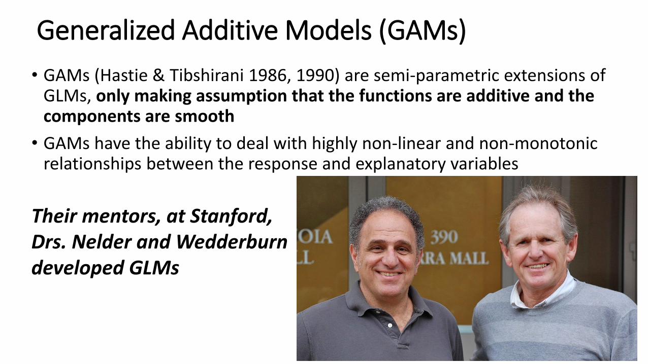
• GAMs (Hastie & Tibshirani 1986, 1990) are semi-parametric extensions of GLMs, only making assumption that the functions are additive and the components are smooth

• GAMs have the ability to deal with highly non-linear and non-monotonic relationships between the response and explanatory variables

Their mentors, at Stanford, Drs. Nelder and Wedderburndeveloped GLMs

Etymology – what’s in a name?

• From Italian word “gamba”

• In those days, it is a slang for a person’s leg, especially an attractive woman’s leg

Linear Regression Models

• Y - response variable X - explanatory variable

• ε - residual error, to cover unexplained information, assumed to be normally distributed with mean of 0 and δ2

• α and β are intercept and slope respectively, to be determined at CI = 95%

• N – sample size

Recall…

Y = α + β1X1 + β2X2 + … + βnXn + ε

When to use GAMs

• When assumptions cannot be made on specific link function for error distribution

• Non-linearity in partial residual plots may suggest semi-parametric modeling

• Priori hypothesis or theory suggest non-linear or skewed relationship among variables

• Shape of predictor functions is determined by the data (Data speak for themselves!!)

Generalized Additive Models• Expressed as:

• Y = α + f(X) + ε where ε ~ N (0,δ2)

• Where βX are replaced with the smoothing curve f(X) which is not defined by an equation, but can be predicted from the model

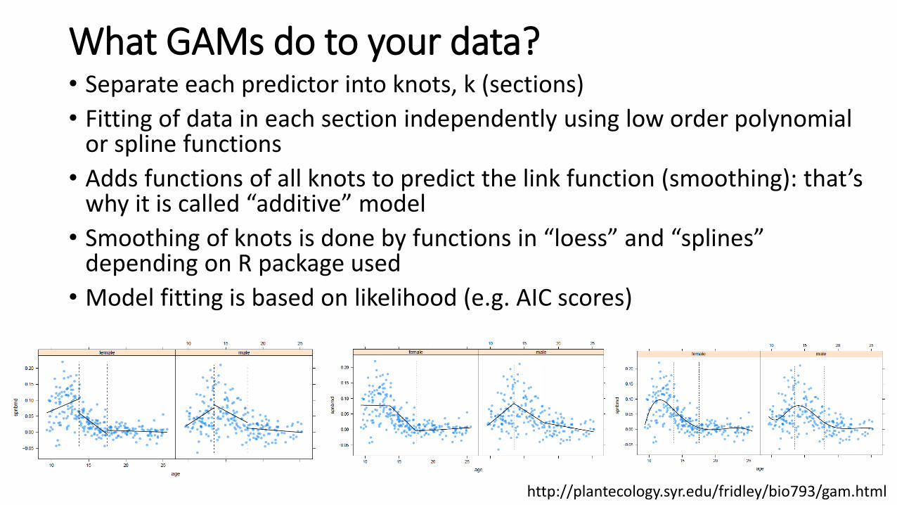
What GAMs do to your data?• Separate each predictor into knots, k (sections)

• Fitting of data in each section independently using low order polynomial or spline functions

• Adds functions of all knots to predict the link function (smoothing): that’s why it is called “additive” model

• Smoothing of knots is done by functions in “loess” and “splines” depending on R package used

• Model fitting is based on likelihood (e.g. AIC scores)

http://plantecology.syr.edu/fridley/bio793/gam.html

Uniqueness of GAMs• A unique aspect of generalized additive models is the non-parametric

(unspecified) function f of the predictor variables x

• Generalized additive models are very flexible, and provide excellent fit for both linear and nonlinear relationships (multiple link functions)

• GAMs can be applied normal distribution as well as Poisson, binomial, gamma and other distributions…

• Regularization of predictor functions helps to avoid over-fitting

Advantages and application of GAMs

• Very powerful for prediction and interpolation

• Highly used in SDMs and ENMs (Elith et al. 2006)

• Analogous to hinge feature of maxent algorithm (Phillips et al. 2006)

• Building optimization models

• Comparatively GAMs shows lower AIC scores and explained higher deviance than GLMs

• Applied in Genetics, epidemiology, molecular biology, air quality and medicine (Dominici et al. 2002)

http://plantecology.syr.edu/fridley/bio793/gam.html

Packages that implement GAMs in R

• gdxrrw (can read or write GDX files)

• mgcv

• gam (old version of mgcv) – requires “splines” package

• mda – “bruto” function

• gamstools

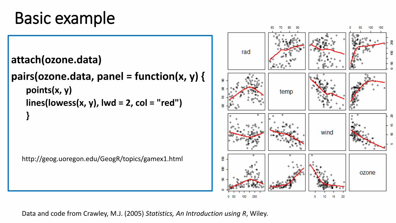
Basic example

attach(ozone.data)

pairs(ozone.data, panel = function(x, y) { points(x, y)

lines(lowess(x, y), lwd = 2, col = "red")

}

Data and code from Crawley, M.J. (2005) Statistics, An Introduction using R, Wiley.

http://geog.uoregon.edu/GeogR/topics/gamex1.html

ozone.gam1 <- gam(ozone ~ s(rad) + s(temp) + s(wind)) summary(ozone.gam1)

“s” is the smoother function added to the covariates

http://geog.uoregon.edu/GeogR/topics/gamex1.html

Significant effect shows evidence of non-linear relationship

plot(ozone.gam1, resid = T, pch = 16)

http://geog.uoregon.edu/GeogR/topics/gamex1.html

wt <- wind * temp ozone.gam2 <- gam(ozone ~ s(temp) + s(wind) + s(rad) + s(wt)) summary(ozone.gam2)

http://geog.uoregon.edu/GeogR/topics/gamex1.html

plot(ozone.gam2, resid = T, pch = 16)

http://geog.uoregon.edu/GeogR/topics/gamex1.html

GAMs has been reported not to handle interactions very well

To investigate how community diversity (measured by Shannon’s Index) is influenced by environmental variables like water quality and sediment

Another example with more functions…

Getting started

Data set collected from 303 stations in estuaries, bays, and tidal rivers located in the Virginian Biogeographic Province (Cape Cod MA to Cape Henry VA) by the U.S. Environmental Protection Agency’s Environmental Monitoring and Assessment Program

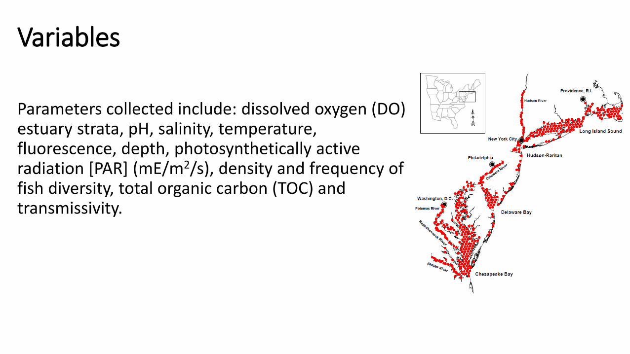
Variables

Parameters collected include: dissolved oxygen (DO), estuary strata, pH, salinity, temperature, fluorescence, depth, photosynthetically active radiation [PAR] (mE/m2/s), density and frequency of fish diversity, total organic carbon (TOC) and transmissivity.

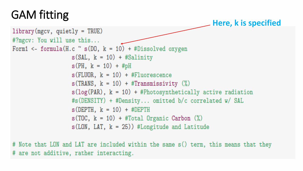
GAM fittingHere, k is specified

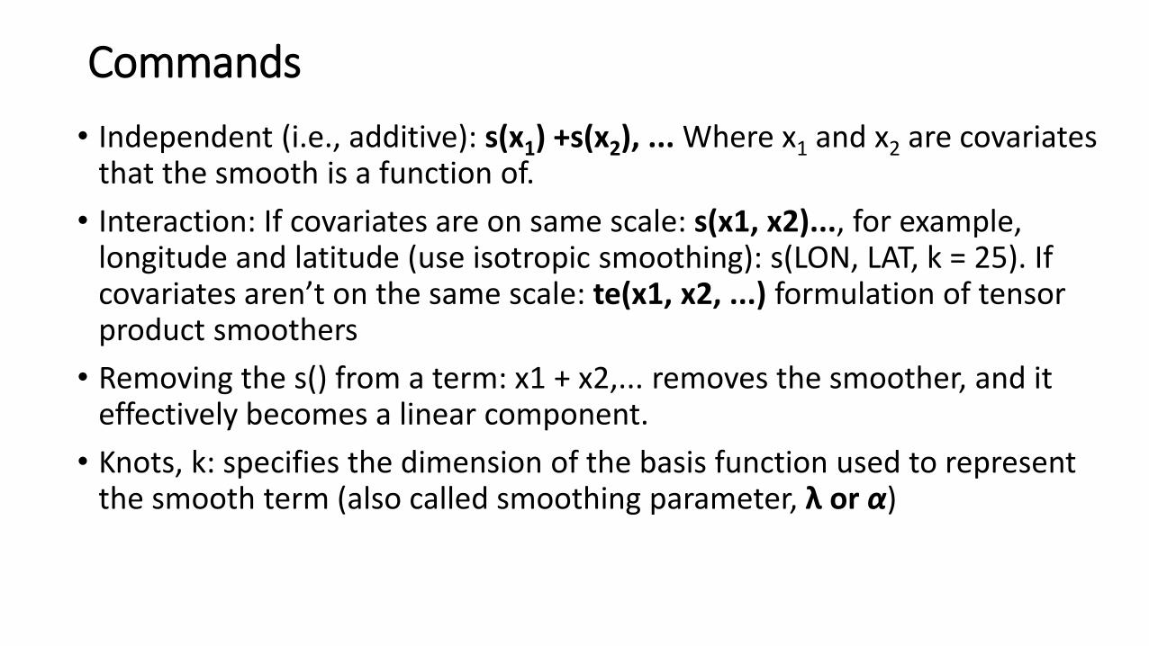
Commands

• Independent (i.e., additive): s(x1) +s(x2), ... Where x1 and x2 are covariates that the smooth is a function of.

• Interaction: If covariates are on same scale: s(x1, x2)..., for example, longitude and latitude (use isotropic smoothing): s(LON, LAT, k = 25). If covariates aren’t on the same scale: te(x1, x2, ...) formulation of tensor product smoothers

• Removing the s() from a term: x1 + x2,... removes the smoother, and it effectively becomes a linear component.

• Knots, k: specifies the dimension of the basis function used to represent the smooth term (also called smoothing parameter, λ or α)

AIC = 523.2

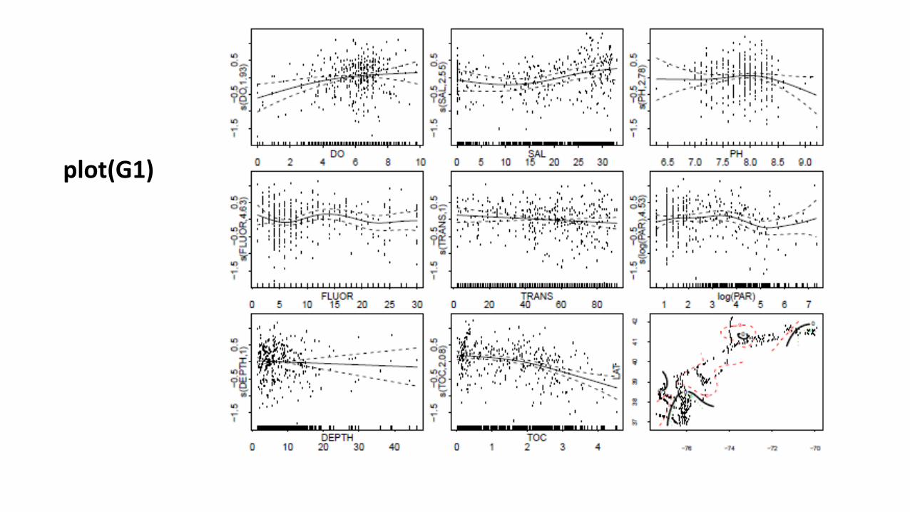
plot(G1)

Using gam.check function, we check how k selection fits the predictors: is it too low or too high?

gam.check or qq.gamproduces residual plots

K selection and overfitting

• If α is too large, we run risk of underfitting, and if α is too small, overfittingcan occur.

• Trade-off in bias (in-sample error) and variance

• Curves with less variance are good for prediction

http://multithreaded.stitchfix.com/blog/2015/07/30/gam/

Smoothing Parameter (λ, k or α)

• There are different methods used to select k:• Cross-validation methods (found in R package mgcv)

• Cross-validation (CV)

• Generalized Cross-validation (GCV)

• Unbiased Risk Estimator (UBRE)

• Likelihood Methods• Restricted Maximum Likelihood (REML)

• Maximum Likelihood (ML)

Explore smooth.terms in “mgcv” package for thorough explanations

How to deal with over-fitting in GAMs

• Model selection with AIC or BIC

• Simple models vs. complex models: curse of dimensionality

• Predictor selection: backward or forward

• Cross validation: 4 or 5-folds (training data)

• Regularization: penalize sources of over-fitting

• Reduce feature space using tools like PCA

• Use bagging (bootstrap aggregation)

• Iterative modelling and play around with k

https://www.quora.com/How-can-I-avoid-overfitting

Iterative modelling until you produce the best fit and optimal k

Degrees of Freedom (df or K’)

• Df is equal to the number of parameters needed to produce the curve, and is calculated by:

• Df = number of knots – 1

• The – 1 part is caused by identification constraint which ensures that all possible predictions from every smoother included in GAM equal to zero

• We use effective degrees of freedom (edf), which is inversely linked with λ, to compare smoothers

• High edf (≥8) means that the curve is non-linear (low λ), edf = 1 is a straight line (high λ)

Very useful resources

• https://stat.ethz.ch/R-manual/R-devel/library/mgcv/html/summary.gam.html

• http://multithreaded.stitchfix.com/blog/2015/07/30/gam/

• https://support.sas.com/rnd/app/stat/topics/gam/gam.pdf

• http://plantecology.syr.edu/fridley/bio793/gam.html

• http://geog.uoregon.edu/GeogR/topics/gamex1.html

• https://rpubs.com/ryankelly/GAMs