Generalized analytic signals in image processing: Comparison

Generalized analytic signals in imageprocessing: Comparison, theory andtheir applications

Swanhild Bernstein, Jean-Luc Bouchot, MartinReinhardt and Bettina Heise

Abstract. This article is intended as both a mathematical overview ofthe generalizations of analytic signals to higher dimensional problems aswell as their applications and comparisons on artificial and real-worldimage samples.

We first start by reviewing the basic concepts behind analytic sig-nal theory and derive its mathematical background based on boundaryvalue problems of one dimensional analytic functions. Based on that,two generalizations are motivated by means of higher dimensional com-plex analysis or Clifford analysis. Both approaches are proven to be validgeneralizations of the known analytic signal concept.

In a last part we experimentally motivate the choice of such higherdimensional analytic or monogenic signal representations in the contextof image analysis. We see how one can take advantage of one or anotherrepresentation depending on the application.

Mathematics Subject Classification (2010). Primary 94A12; Secondary44A12, 30G35.

Keywords. Monogenic signal, monogenic functional theory, image pro-cessing, texture, Riesz transform.

1. Introduction

In the past years and since the pioneer work of Gabor [10], the analytic signalhas attracted manifold interests in signal processing and information theory.Due to an orthogonal decomposition of oscillating signals into envelope andinstantaneous phase or respectively into energetic and structural components,this concept has become very suitable for analyzing signals. In this contextsuch a property is called a split of identity and allows to separate the differentcharacteristics of a signal into useful components.

2 Bernstein, Bouchot, Reinhardt and Heise

While this approach has given rise to many one dimensional signal pro-cessing methods, other developments have been directed towards higher di-mensional generalizations. Of particular interest is the two dimensional case,i.e.how to deal with images in an analytic way. As it will be demonstrated inour paper, two main directions have been taken, one based on multidimen-sional complex analysis and another one based on Clifford analysis.

This article is intended as an overview of the mathematical conceptsbehind analytic signals based on the Hilbert transform (Sec. 2). Then, themathematical generalizations are detailed in Sec. 3. The end of that sectionis dedicated to illustrative examples of the differences between the two gen-eralizations detailed. Sec. 4 describes the use of spinors for image analysistasks. The last section of this article (Sec. 5) illustrates their applicationslike demodulation of two dimensional AM-FM signals as provided e.g. ininterferometry and some applications in natural images processing.

2. Analytic signal theory and signal decomposition

Analytic signals have been introduced for signal processing in the context ofcommunication theory in the late 40s [10]. Since then, it has shown growinginterest as a useful tool for representing real valued signals [23]. We starthere by first reviewing the basics about analytic signal theory and Hilberttransform and see how the so-called split of identity is an interesting property.In the last part we review the mathematical basics and see how we can derivethe analytic signal from a boundary value problem in complex analysis.

2.1. Basic analytic signal theory and the Hilbert transform

Definition 2.1 (1 Dimensional Fourier Transform). In the following, we useas Fourier transform F :

F(f)(u) = f(u) =1√2π

∫Rf(t)e−itudt (2.1)

for t ∈ R, u ∈ R and f ∈ L2(R)

Definition 2.2 (Hilbert Transform). The Hilbert transform of a signal f ∈L2(R) (or more generally f ∈ Lp(R), 1 < p < ∞) is defined either in thespatial domain as a convolution with the Hilbert kernel 2.2 or as a Fouriermultiplier 2.3:

Hf = h ∗ f (2.2)

F(Hf)(u) = −i sign(u)F(f)(u) (2.3)

where we have made use of two functions:

• The Hilbert kernel h(t) = 1πt

• The operator sign(u) =

1 u > 00 u = 0−1 u < 0

Generalized analytic signals in image processing 3

Following its definition, we notice that the Hilbert transform acts as anasymmetric phase shifting: if we write ±i = e±iπ/2, the phase of the Fourierspectrum of the Hilbert is obtained by a rotation of ±90◦.

Proposition 2.3 (Properties of the Hilbert Transform). Given a signal f thefollowings hold true:

• ∀u 6= 0, |Hf(u)| = |F(f)(u)|• HHf = −f ⇒ H−1 = −H

Note that a constant function being not in L2 can not be reconstructed thatway.

The analytic signal is computed as a complex combination of both orig-inal signal and its Hilbert transform:

Definition 2.4 (Analytic Signal).

fA = f + iHf (2.4)

Due to its definition, an analytic signal has a one sided Fourier spectrum.And moreover, we have that its values are doubled on the positive side. Wecan also remark that it is possible to recover the original signal based on itsanalytic description by taking the real part.

It holds:

Proposition 2.5.

〈f,Hf〉L2= 0 Orthogonality (2.5)

‖f‖22 = ‖Hf‖22 Energy (2.6)

The energy equality is valid only if the DC component of the signal isneglected [9].

Note that it is possible to write the complex analytic signal in polarcoordinate. In this case we have: ∀t ∈ R, fA(t) = A(t)eiφ(t) A is called thelocal amplitude and φ is called the local phase. These local features aredefined as follows [10]:

Definition 2.6 (Local features).

A(t) =√f(t)2 +Hf(t)2 (2.7)

φ(t) = arctan

(Hf(t)

f(t)

)= arctan

(= (fA(t))

< (fA(t))

)(2.8)

Proposition 2.7 (Invariance - equivariance, Split of identity [9]). The localphase together with the local amplitude fulfill the property of invariance-equivariance:

• The local phase depends only on the local structure• The local amplitude depends only on the local energy

If moreover these features are a complete description of the signal, theyare said to perform a split of identity.


However as stated in [9], the split of identity is strictly valid only forband-limited signals with local zero mean property.

If these conditions are fulfilled the analytic signal representation relies onan orthogonal decomposition of the structural information (the local phase),and the energetic information (the local amplitude).

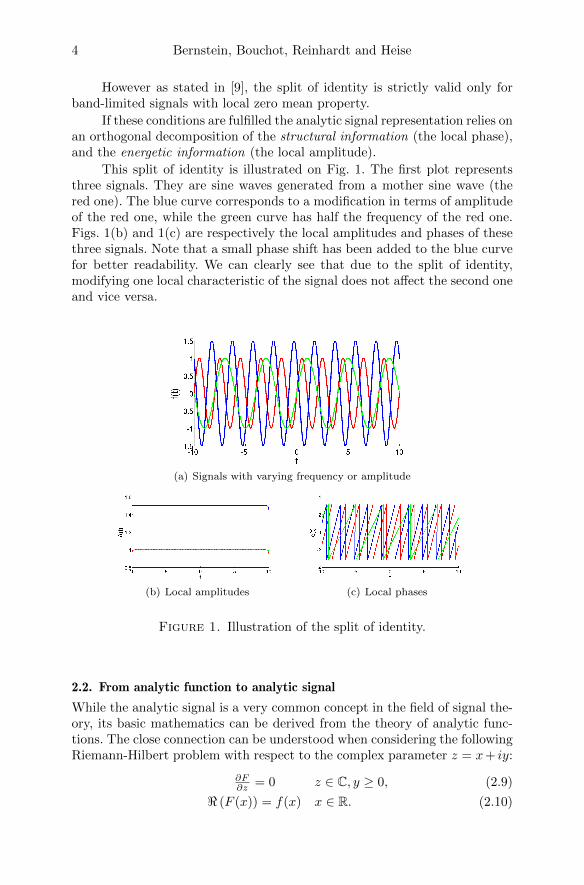
This split of identity is illustrated on Fig. 1. The first plot representsthree signals. They are sine waves generated from a mother sine wave (thered one). The blue curve corresponds to a modification in terms of amplitudeof the red one, while the green curve has half the frequency of the red one.Figs. 1(b) and 1(c) are respectively the local amplitudes and phases of thesethree signals. Note that a small phase shift has been added to the blue curvefor better readability. We can clearly see that due to the split of identity,modifying one local characteristic of the signal does not affect the second oneand vice versa.

(a) Signals with varying frequency or amplitude

(b) Local amplitudes (c) Local phases

Figure 1. Illustration of the split of identity.

2.2. From analytic function to analytic signal

While the analytic signal is a very common concept in the field of signal the-ory, its basic mathematics can be derived from the theory of analytic func-tions. The close connection can be understood when considering the followingRiemann-Hilbert problem with respect to the complex parameter z = x+ iy:

∂F∂z = 0 z ∈ C, y ≥ 0, (2.9)

< (F (x)) = f(x) x ∈ R. (2.10)


One solution of this problem is given by the Cauchy integral

F (z) = FΓf(z) :=1

2πi

∫R

1

τ − zf(τ)dτ. (2.11)

Of course this solution is unique only up to a constant. Normally, this constantwill be fixed by the condition = (F (z0)) = c, i.e.the imaginary part of F givenin an interior point.

When we now consider the trace of FΓ, i.e. the boundary value, wearrive at the so-called Plemelj-Sokhotzki formula:

trFΓf =1

2(I + iH)f =

1

2f +

1

2iHf =: PΓf. (2.12)

Up to the factor 1/2 this corresponds to our above definition of an analyticsignal.

In this way an analytic signal represents the boundary values of ananalytic function in the upper half plane (or for periodic functions in theunit disc). Starting from this concept we are going now to take a look athigher dimensional generalizations.

3. Higher dimensional generalizations

Different approaches have been studied in the past years to extend the defi-nition of an analytic signal to higher dimensional spaces. Two of them havegained the greatest interest based respectively on multidimensional complexanalysis and Clifford analysis.

3.1. Using multiple complex variables

3.1.1. Mathematics. In 1998 Bulow proposed a definition of a hypercomplexsignal based on the so-called partial and total Hilbert transform [5]. To lookfrom our point of view that analytic signals are functions in a Hardy spacewe consider the following Riemann-Hilbert problem in C2:

∂F∂z1

= 0 (z1, z2) ∈ C2, y1, y2 ≥ 0, (3.1)

∂F∂z2

= 0 (z1, z2) ∈ C2, y1, y2 ≥ 0, (3.2)

< (F (x1, x2)) = f(x1, x2) x1, x2 ∈ R2. (3.3)

For the solution, (see e.g. [7] or [20]), we just want to point out that thedomain is a poly-domain in the sense of Cn, so that we can give it in form ofthe Cauchy integral:

F (z1, z2) =1

4π2

∫R2

1

(ξ1 − z1)(ξ2 − z2)f(ξ1, ξ2)dξ1dξ2. (3.4)

Now again looking at the corresponding Plemelj-Sokhotzki formula weget

trF (x1, x2) = 14f(x1, x2)− 1

4

∫R2

1(ξ1−x1)(ξ2−x2)f(ξ1, ξ2)dξ1dξ2

+i 14

(∫R

1ξ1−x1

f(ξ1, x2)dξ1 +∫R

1ξ2−x2

f(x1, ξ2)dξ2

)(3.5)


which up to the factor 1/4 corresponds to the definition of an analytic signalby Hahn [12]. Here

Hif =

∫R

1

ξi − xif(ξi, ·)dξ1 (3.6)

is called the partial Hilbert transform and

HT f =1

4

∫R2

1

(ξ1 − x1)(ξ2 − x2)f(ξ1, ξ2)dξ1dξ2 (3.7)

the total Hilbert transform. On the level of Fourier symbols we get

F(trF )(u1, u2) = (1 + signu1)(1 + signu2)Ff(u1, u2). (3.8)

Let us now take a look at the definition of Bulow. To this end we considerF to be a function of two variables z1 and z2 with two different imaginaryunits i and j (with i2 = j2 = −1), i.e. z1 = x1 + iy1 and z2 = x2 + jy2.We remark that both imaginary units can be understood as elements of thequaternionic basis with multiplication rules ij = −ji = k. In this way theabove Riemann-Hilbert problem can be rewritten as

∂∂z1

F = 0 (z1, z2) ∈ C2, y1, y2 ≥ 0, (3.9)

F ∂∂z2

= 0 (z1, z2) ∈ C2, y1, y2 ≥ 0, (3.10)

< (F (x1, x2)) = f(x1, x2) x1, x2 ∈ R2, (3.11)

where the second equation should be understood as ∂z2 being applied fromthe from the right due to the non-commutativity of the complex units i andj.

The solutions is given by

F (z1, z2) =1

4π2

∫R2

1

(ξ1 − z1)(ξ2 − z2)f(ξ1, ξ2)dξ1dξ2 (3.12)

so that we get from the Plemelj-Sokhotzki formulae

trF (x1, x2) =1

4(I + iH1)(I + jH2)f(x1, x2) (3.13)

=1

4(f + iH1f + jH2f + kHT f)(x1, x2). (3.14)

While this is now a quaternionic-valued function, it still corresponds to aboundary value of a function holomorphic in two variables. For the repre-sentation in Fourier domain one has to keep in mind that now one has toapply one Fourier transform with respect to the complex plane in i and oneFourier transform with respect to the complex plane generated by j. Takinginto account that ij = −ji one arrives at the so-called quaternionic Fouriertransform [15, 5]:

QFf =

∫R2

eix1ξ1f(x1, x2)ejx2ξ2dx1dx2 (3.15)

and the following representation in Fourier symbols


QF(trF )(u1, u2) = (1 + signu1)(1 + signu2)QFf(u1, u2) (3.16)

3.1.2. Image analysis. In image analysis problems, according to [12] we canintroduce the following featuresAmplitude. The local amplitude of a multidimensional analytic signal is de-fined in a similar way as for the one-dimensional case:

AA(x, y) =√|f(x, y)|2 + |H1f(x, y)|2 + |H2f(x, y)|2 + |HT f(x, y)|2 (3.17)

This is also denoted as energetic informationPhase. The phase is a feature describing how much a vector or quaternionnumber diverge from the real axis. It is defined in a similar manner as for theclassical complex plane.

φA = arctan

(√H1f2 +H2f2 +HT f2

f

)(3.18)

This angle φA is what is denoted as phase or structural information.Orientation. As we are at the moment interested in 2D signals (=images),we can also describe an orientation information, as the principal directioncarrying the phase information. The imaginary plane, spanned by {i, j}, istwo-dimensional and therefore we can also define an angle θA in this plane:

θA = arctan

(H2f

H1f

)(3.19)

This new angle is called the orientation of the signal or geometric in-formation.

3.2. Using Clifford analysis

Another approach to higher dimensions is the so-called Clifford analysis.

3.2.1. Mathematics. Here we use a so-called Clifford algebra C`0,n [3]. Thisis the free algebra constructed over Rn generated modulo the relation

x2 = −|x|2e0 x ∈ Rn (3.20)

where e0 is the identity of C`0,n. For the algebra C`0,n we have theanti-commutation relationship

eiej + ejei = −2δije0, (3.21)

where δij is the Kronecker symbol. Each element x of Rn may be rep-resented by

x =

n∑i=1

xiei. (3.22)

A first-order differential operator which factorizes the Laplacian is givenas the so-called Dirac operator


Df(x) =

n∑j=1

∂f

∂xj. (3.23)

The Riemann-Hilbert problem for the Dirac operator can be stated inthe form

DF (x) = 0 x ∈ R3, x3 > 0 (3.24)

< (F (x1, x2)) = f(x1, x2) x1, x2 ∈ R2 (3.25)

To solve this problem we follow the same idea as above.

FΓf =

∫R2

x− y|x− y|2

e3f(x1, x2)dx1dx2 (3.26)

trFΓf =1

2(I + SΓ)f =

1

2f(y1, y2)

+1

2

∫R2

e1(x1 − y1) + e2(x2 − y2)

|x− y|2e3f(x1, x2)dx1dx2. (3.27)

Because the quaternions H are isomorphic to the even subalgebra C`+0,3,i.e. all elements of the form

c0 + c1e1e2 + c2e1e3 + c3e2e3, c0, c1, c2, c3 ∈ R (3.28)

we can set i = e1e2 and j = e2e3 so that

trFΓf =1

2(I + SΓ)f (3.29)

=1

2f(y1, y2) +

1

2

∫R2

i(x1 − y1) + j(x2 − y2)

|x− y|2f(x1, x2)dx1dx2.

(3.30)

Up to the factor 1/2 this is the monogenic signal fM = f + iR1f +jR2f := f + (i, j)Rf of Sommer and Felsberg [9]. Here R1, R2 and Rdenote respectively the first and second component of the Riesz transform,and the Riesz transform itself [22]. Defined as Fourier multipliers, it holds:

Rf(u1, u2) =i(u1, u2)

‖(u1, u2)‖2f(u1, u2) (3.31)

R1f(u1, u2) =iu1

‖(u1, u2)‖2f(u1, u2) (3.32)

R2f(u1, u2) =iu2

‖(u1, u2)‖2f(u1, u2) (3.33)

where ‖(u1, u2)‖2 =√u2

1 + u22.

or equivalently defined in the spatial domain by convolution with the2-dimensional Riesz kernel, for m = 1, 2

Rif = cxi‖x‖32

∗ f (3.34)


with c being a constant.

3.2.2. Image analysis. Following [9] three features can be computed and willbe denoted as energetic, structural and geometrical information too, as al-ready introduced for the multidimensional analytic signal.Amplitude. The local amplitude of a monogenic signal is defined in a similarway as for the analytic signal:

AM (x, y) =√|f(x, y)|2 + |Rf(x, y)|2 =

√fM (x, y)fM (x, y) (3.35)

where the · denotes the conjugation of a quaternion.Phase.

φM (x, y) = arctan|Rf(x, y)|f(x, y)

(3.36)

and we still have that φM denotes the angle between A(x, y) and fM(in the plane spanned by the two complex vectors). This yields values φM ∈[−π/2;π/2]

An alternative equivalent definition is using arccos:

φM = arccosf

|fM |(3.37)

In this case, we have φM ∈ [0;π]Orientation. Once again, we can derive an orientation θM ∈ [−π, π] based onthe monogenic signal which represents the direction of the phase information.

θM = arctanR2f

R1f(3.38)

We note that this definition actually only provides an orientation mod. π.To determine the orientation resp. direction mod. 2π it needs a further ori-entation unwrapping step or sign estimation [17, 4].

3.3. Illustrations

We want here to illustrate the differences between the generalizations pro-posed. We will visually assess the characteristics of both approaches firstfacing a Siemens star1 then facing a checkerboard image. Both examples areinteresting for their regularity (point symmetry for the star and many hori-zontal and vertical line symmetries for the checkerboard).

An example of such star is depicted on Fig. 2(a). The two other imagesof first row from Fig. 2 illustrate the two components of the Riesz transform.As we can see, and we will come back on that property later, the partial Riesztransforms show in some point a similar behavior as steered derivatives. Thefirst component tends to emphasize horizontal edges while the second onetends to respond more to vertical ones.

The second row shows the results applying the different Hilbert trans-forms to the Siemens star. The two first images represent the results of the

1The Siemens star is a known test image to characterize the resolution of different op-

tical/graphical devices such as printers or beamers. It is interesting as it shows lots ofregularity, many intrinsic one dimensional and two dimensional parts.


two partial Hilbert transforms and the last one depicts the results after thetotal Hilbert transform. We can notice the high anisotropy of these transformsat, for instance, the strong vertical resp. horizontal delimitation through thecenters of the images. We can also notice the patchy responses of the totalHilbert transform.

As the Riesz kernel in polar coordinate [r, α] of the spatial domain reads

R(r, α) ∼ 1

r2eiα (3.39)

it exhibits an isotropic behavior with respect to its magnitude. In comparison,the partial and the total Hilbert transforms induce a strict relationship to theorthogonal coordinate system and therefore also the two-dimensional analyticsignal is coined in such a way.

(a) Siemens star (b) First compo-nent of the Riesz

transform

(c) Second compo-nent of the Riesz

transform

(d) First Hilberttransform

(e) Second Hilberttransform

(f) Total Hilberttransform

Figure 2. The Siemens star together with the differentRiesz and Hilbert transforms presented in this section.

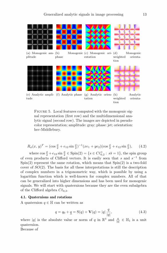
Next we consider the local features computed according to the formulasintroduced above. The results are depicted in Fig. 3. The first row corre-sponds to monogenic features, while the second one corresponds to analyticfeatures. The phase is displayed in a jet colormap, the orientation in an hsvcolormap. The last column shows the orientations whose intensity is weightedproportionally to the cosine of the phase. It is shown according to Middle-bury’s representation2: strength (cosine of the phase) is encoded as an in-tensity value of the color and the color itself corresponds to the orientation.

2Middlebury benchmark for optical flow is a web resource for comparing results on optical

flow computations. The color error representation is well suited for encoding our orienta-tion. More info can be found at http://vision.middlebury.edu/flow/


The main differences between these two sets of features lie in the shape orboundaries. While monogenic features yield rather smooth boundaries, theanalytic representation creates abrupt changes due to its anisotropy. We canremark how the phase gives reasonable insights about the structures in theimages.

(a) Monogenic am-

plitude

(b) Monogenic

phase

(c) Monogenic ori-

entation

(d) Phase weighted

monogenic orienta-tion

(e) Analytic ampli-tude

(f) Analytic phase (g) Analytic orien-tation

(h) Phase weightedanalytic orientation

Figure 3. Local features computed with the monogenic sig-nal representation (first row) and the multidimensional ana-lytic signal (second row). The images are depicted in pseudo-color representation; amplitude: gray; phase: jet; orientation:hsv-Middlebury.

In comparison to the Siemens star, the checkerboard example (see Fig. 4(a))shows many orthogonal features. In this case, we see that the partial Hilberttransforms give some good insights of the closeness of an edge and preservesthe checkerboard structure (Fig. 4(d) and 4(e)) while the Riesz transformgives more local responses. The total Hilbert transform acts as an accuratecorner detection, as it can be seen from its response on Fig. 4(f).

When discussing the analytic and monogenic features (Fig. 5) we re-mark that this effect is preserved. The Riesz transform being well localize atthe edges does not yield many differences inside one of the square and seemsto jump from an extreme to another through those edges. See in particu-lar Fig. 5(b) for an illustrative example of the phase. On the other side, theHilbert transform containing more neighborhood information yields smoothertransition in the phase from a square to another. This idea has to be consid-ered carefully based on the applications one wants to solve.


(a) Checkerboardimage

(b) First compo-nent of the Riesz

transform

(c) Second compo-nent of the Riesz

transform

(d) First Hilberttransform

(e) Second Hilberttransform

(f) Total Hilberttransform

Figure 4. The checkerboard together with the differentRiesz and Hilbert transforms presented in this section.

4. The geometric approach

For a better understanding of signals a geometric interpretation of a signalcan help. The following considerations about complex numbers, quaternions,rotations, the unitary group, the special unitary and special orthogonal groupas well as the spin group are well-known and can be found in numerouspapers. We would like to suggest the book [18], as a comprehensive insightin the topic. The analytic signal fA(t) = A(t)eiφ(t) are boundary values ofan analytic function, but the analytic signal can also be seen as a complexnumber, where eiφ(t) = cosφ(t) + i sinφ(t) has modulus 1 and hence can beidentified with the unit circle S1. But there is even more. The set of unitcomplex numbers becomes a group with the complex multiplication whichis the unitary group U(1) = {z ∈ C : zz = 1}. On the other hand a unitcomplex number can also be seen as a rotation in R2 if we identify the unitcomplex number with the matrix

Rφ =

(cosφ − sinφsinφ cosφ

)∈ SO(2) (4.1)

the group of all counter-clockwise rotations in R2. Now everything can also bedescribed inside Clifford algebras. Let us consider the Clifford algebra C`0,2with generators e1, e2. The complex numbers can be identified with all ele-ments x+ye12, x, y ∈ R, i.e. the even subalgebra C`+0,2 of the Clifford algebra

C`0,2. The rotation (4.1) can also be described by a Clifford multiplication.To see that we identify (x, y) ∈ R2 with xe1 + ye2 ∈ C`0,2 and


(a) Monogenic am-plitude

(b) Monogenicphase

(c) Monogenic ori-entation

(d) Monogenicweighted orienta-

tion

(e) Analytic ampli-tude

(f) Analytic phase (g) Analytic orien-tation

(h) Analyticweighted orienta-

tion

Figure 5. Local features computed with the monogenic sig-nal representation (first row) and the multidimensional ana-lytic signal (second row). The images are depicted in pseudo-color representation; amplitude: gray; phase: jet; orientation:hsv-Middlebury.

Rφ(x, y)T = (cos φ2 + e12 sin φ2 )−1(xe1 + ye2)(cos φ2 + e12 sin φ

2 ), (4.2)

where cos φ2 +e12 sin φ2 ∈ Spin(2) = {s ∈ C`+0,2 : ss = 1}, the spin group

of even products of Clifford vectors. It is easily seen that s and s−1 fromSpin(2) represent the same rotation, which means that Spin(2) is a two-foldcover of SO(2). The basis for all these interpretations is still the descriptionof complex numbers in a trigonometric way, which is possible by using alogarithm function which is well-known for complex numbers. All of thatcan be generalized into higher dimensions and has been used for monogenicsignals. We will start with quaternions because they are the even subalgebraof the Clifford algebra C`0,3.

4.1. Quaternions and rotations

A quaternion q ∈ H can be written as

q = q0 + q = S(q) + V(q) = |q| q|q|, (4.3)

where |q| is the absolute value or norm of q in R4 and q|q| ∈ H1 is a unit

quaternion.Because of


∣∣∣∣ q|q|∣∣∣∣2 =

3∑i=0

q2i

|q|2= 1, (4.4)

the set of unit quaternions H1 can be identified with S3, the threedimensional sphere in R4.On the other hand the Clifford algebra C`0,3 is generated by the elementse1, e2 and e3 with e2

1 = e22 = e2

3 = −1 and eiej + ejei = −2δi,j . Its evensubalgebra C`+0,3, as defined in 3.28, can be identified with quaternions bye1e2 ∼ i, e1e3 ∼ j and e2e3 ∼ k.Furthermore,

Spin(3) = {u ∈ C`+0,3 : uu = 1} = H1. (4.5)

That means a unit quaternion can be considered as a spinor. BecauseSpin(3) is a double cover of the group SO(3), rotations can be described byunit quaternions. The monogenic signal is interpreted as a spinor in [24] andlately in [1].

4.2. Quaternions in trigonometric form

The analytic signal is a holomorphic/analytic function and therefore con-nected to complex numbers. Complex numbers can be written in algebraicor trigonometric form:

z = x+ iy = reiφ.

The analytic signal is given by

A(t)eiφ(t)

with amplitude A(t) and (local) phase φ(t). We want to obtain a similarrepresentation of the monogenic signal by quaternions. A simple computationleads to

q = |q|(q0

|q|+

q

|q||q||q|

)= |q|(cosφ+ u sinφ),

where φ = arccos q0|q| and u =

q

|q| ∈ S2. (Alternatively, the argument φ can be

defined by the arctan.)We can represent the quaternion q by its amplitude |q|, the phase φ and theorientation u. Moreover,

q = |q| euφ,

where e is the usual exponential function.By the aid of an appropriate logarithm we can compute uφ from q

|q| =

euφ. Next, we want to explain the orientation u. We already got that

q = |q|(cosφ+ u sinφ),

where u =q

|q| ∈ S2 and u2 = −1, i.e. u behaves like a complex unit. But

because u ∈ S2 we can u express in spherical coordinates. We have

u =q1i + q2j + q3k

|q1i + q2j + q3k|= i

(q1

|q|+

(q2(−ij) + q3j)

|q|

)(4.6)


and if we set cos θ = q1|q| we get

u = i(cos θ + u sin θ), u =q

|q|and q = jq3 − ijq2. (4.7)

Because of

q = jq3 − ijq2 = j(q3 + iq2) (4.8)

and with cos τ = q3|q| we get that

u = j(cos τ + i sin τ). (4.9)

Finally, we put everything together and obtain

q = q0 + q1i + q2j + q3k (4.10)

= |q|(cosφ+ u sinφ) = |q|(cosφ+ i

(cos θ + u sin θ

)sinφ

)(4.11)

= |q| (cosφ+ i (cos θ + j (cos τ + i sin τ) sin θ) sinφ) (4.12)

= |q| (cosφ+ i sinφ cos θ + j sinφ sin θ sin τ + k sinφ sin θ cos τ) , (4.13)

where φ, θ ∈ [0, π] and τ ∈ [0, 2π]. In case of a reduced quaternion, i.e. q3 =0, a similar computation leads to

q = q0 + q1i + q2j (4.14)

= |q| (cosφ+ u sinφ) = |q| (cosφ+ i (cos θ − k sin θ) sinφ) (4.15)

= |q| (cosφ+ i sinφ cos θ + j sinφ sin θ) , (4.16)

where φ ∈ [0, π] and θ ∈ [0, 2π].It is easily seen that θ can be computed by

tan θ =q2

q1⇐⇒ θ = arctan

q2

q1.

If we compare that with the monogenic signal

fM (x, y) = f(x, y) + i(R1f)(x, y) + j(R2f)(x, y)

we see that (compare with 3.38)

θ = arctan(R2f)(x, y)

(R1f)(x, y)= θM (x, y). (4.17)

Therefore the vector u = i cos θ+ j sin θ can also be considered as the orien-tation.

4.3. Exponential function and logarithm for quaternionic arguments

The exponential function for quaternions and para-vectors in a Clifford alge-bra are defined in [11] and many other papers.

Definition 4.1. For q ∈ H is the exponential function defined as

eq :=

∞∑k=0

qk

k!. (4.18)


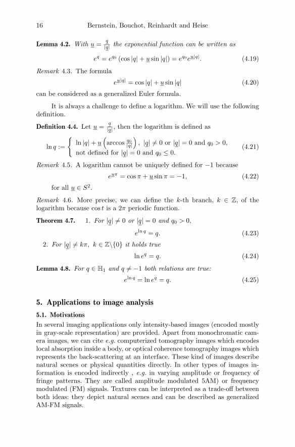
Lemma 4.2. With u =q

|q| the exponential function can be written as

eq = eq0 (cos |q|+ u sin |q|) = eq0eu|q|. (4.19)

Remark 4.3. The formula

eu|q| = cos |q|+ u sin |q| (4.20)

can be considered as a generalized Euler formula.

It is always a challenge to define a logarithm. We will use the followingdefinition.

Definition 4.4. Let u =q

|q| , then the logarithm is defined as

ln q :=

{ln |q|+ u

(arccos q0

|q|

), |q| 6= 0 or |q| = 0 and q0 > 0,

not defined for |q| = 0 and q0 ≤ 0.(4.21)

Remark 4.5. A logarithm cannot be uniquely defined for −1 because

euπ = cosπ + u sinπ = −1, (4.22)

for all u ∈ S2.

Remark 4.6. More precise, we can define the k-th branch, k ∈ Z, of thelogarithm because cos t is a 2π periodic function.

Theorem 4.7. 1. For |q| 6= 0 or |q| = 0 and q0 > 0,

eln q = q. (4.23)

2. For |q| 6= kπ, k ∈ Z\{0} it holds true

ln eq = q. (4.24)

Lemma 4.8. For q ∈ H1 and q 6= −1 both relations are true:

eln q = ln eq = q. (4.25)

5. Applications to image analysis

5.1. Motivations

In several imaging applications only intensity-based images (encoded mostlyin gray-scale representation) are provided. Apart from monochromatic cam-era images, we can cite e.g. computerized tomography images which encodeslocal absorption inside a body, or optical coherence tomography images whichrepresents the back-scattering at an interface. These kind of images describenatural scenes or physical quantities directly. In other types of images in-formation is encoded indirectly , e.g. in varying amplitude or frequency offringe patterns. They are called amplitude modulated 5AM) or frequencymodulated (FM) signals. Textures can be interpreted as a trade-off betweenboth ideas: they depict natural scenes and can be described as generalizedAM-FM signals.


To enrich the information content of pure intensity image (i.e. imagesencoded with a single value at each pixel), we test the concept of analyticsignals in image processing.

5.2. Application to AM-FM images demodulation

Here we study the applicability of the monogenic signal representation toAM-FM signal demodulation, as needed for instance in interferometric imag-ing [17]. A certain given two dimensional signal (= an image, Fig. 6(a))exhibits both amplitude modulations (Fig. 6(b)) and frequency modulations(Fig. 6(c)). The aim is to separate each components of the signal by meansof monogenic signal analysis.

(a) Original AM-

FM image

(b) Amplitude

modulations

(c) Frequency mod-

ulations

(d) Reconstructed

orientation

(e) Reconstructed

amplitude

(f) Reconstructed

phase

Figure 6. Example of a two dimensional AM-FM signal.The first row shows the input ground truth image togetherwith its amplitude and frequency modulations. The secondrow depicts the recovered orientation, amplitude and phases.Images are displayed using conventional jet colormap.

The three features described in the previous section are computed andtheir results are depicted on Fig. 6(d) (local orientation), Fig. 6(e) (localamplitude) and Fig. 6(f) (local phase).

It appears that on such AM-FM signals, the orientation is able to de-scribe the direction of the phase modulation, while the local amplitude givesa good approximation of the amplitude modulation (corresponding to the en-ergy of the two dimensional signal) and the phase encodes information aboutthe frequency modulation (understood as the structural information).

The next example shows a fringe pattern as an example of real-worldinterferometrice AM-FM image, Fig. 7(a).


(a) Fringe pattern (b) Monogenic lo-

cal phase

(c) Monogenic local

orientation

(d) Monogenic lo-cal amplitude

(e) Masked phase (f) Masked orienta-tion

Figure 7. Example of a fringe pattern and its monogenicdecomposition. Phase (second column) is encoded as a jetcolormap and orientation as hsv. The two last images showphase and orientation masked with a binary filter set to onewhen the local amplitude gets over a certain threshold.

The following images show the monogenic analysis of this image. Be-neath the fringe pattern (Fig. 7(d)) the local amplitude is depicted. Thisimage gives us a coarse idea of how much structure is to be found on a givenneighborhood. The second column illustrates the phase calculation either onthe whole image (Fig. 7(b)) or only where the local amplitude is above a giventhreshold (Fig. 7(e)). The two last images represent the monogenic orienta-tion encoded in hsv with or without the previous mask. As we would expect,illumination changes are appearing in the amplitude while local structuresare contained in both phase and orientation features.

5.3. Application to texture analysis

A task of particular interest in artificial vision, is the characterization ordescription of textures. The problem here is to find interesting features todescribe a given texture the best we can in order to classify it for instance [13].The use of steerable filters could optimize the feature computations and affectthe classification. In other words, if we can compute well describing features,we can better characterize a texture.

Considering textures from a more general viewpoint as almost AM-FM signals, we examine here the use of monogenic representation for localcharacterization of a textured object depicted in Fig. 8(a).

When looking at the monogenic signal’s local description (amplitudeon Fig. 8(b), phase on Fig. 8(c) and orientation on Fig. 8(d)) we indeed see


(a) Original texture (b) Monogenic am-plitude

(c) Monogenicphase

(d) Monogenic ori-entation

Figure 8. Example of a textured image superposed by areliability mask together with its monogenic analysis; regionswith too little amplitude are masked out to be unreliable.

these repetitive features along the textured object. Moreover, these estimatedvalues seem to be robust against small imperfection in the periodicity.

5.4. Applications to natural image scenes

In this part of work, we want to give some ideas of the interest of the mono-genic signal for natural images. Such images have completely different char-acteristics as the ones introduced above. For instance, images are often em-bedded in full cluttered background, encoded on more color channels, haveinformation at many different scales... In practical applications one needs toapply band-pass filters before analyzing such images [9]. Note that this workconsiders only gray-scaled images, but literature can be found in order todeal with multichannel images [2].

We will in the followings describe two tasks useful for image processing.The first part deals with edge detection. We see how the Riesz transformcan be used as an edge detector in images. Then we see how the orienta-tion estimation is useful for instance in computer vision tasks and how themonogenic signal analysis can help for this, as it has already been done forstructure interpretation [21, 14].

5.4.1. Edge detection. The Riesz transform can be seen as an edge detectorsfor several reasons. It appears clearly when one has a closer look at its def-inition as a Fourier multiplier. Indeed, let us recall the jth Riesz multiplier(see Eq. 3.31):

Rjf = iuj|u|f (5.1)

and we have

Rjf = i1

|u|∂jf (5.2)

so that the Riesz transform acts as a normalized derivative operator.Another (eventually better) way to see this derivative effect is to con-

sider the Fourier multipliers in polar coordinates [16], which is given byEq.3.39 .

Fig. 9 illustrates this behavior.


(a) Lena image (b) Lena’s first

Riesz component

(c) Lena’s second

Riesz component

(d) Barbara image (e) Barbara’s firstRiesz component

(f) Barbara’s sec-ond Riesz compo-

nent

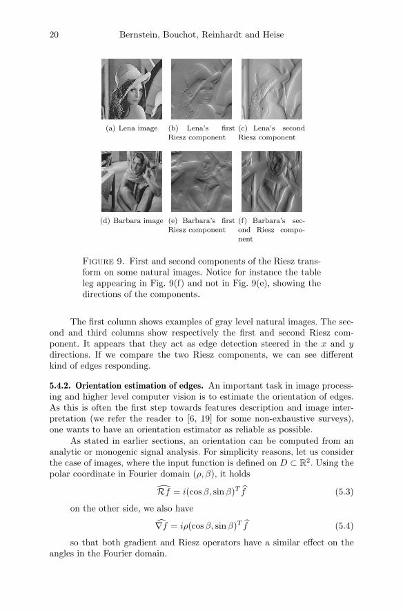
Figure 9. First and second components of the Riesz trans-form on some natural images. Notice for instance the tableleg appearing in Fig. 9(f) and not in Fig. 9(e), showing thedirections of the components.

The first column shows examples of gray level natural images. The sec-ond and third columns show respectively the first and second Riesz com-ponent. It appears that they act as edge detection steered in the x and ydirections. If we compare the two Riesz components, we can see differentkind of edges responding.

5.4.2. Orientation estimation of edges. An important task in image process-ing and higher level computer vision is to estimate the orientation of edges.As this is often the first step towards features description and image inter-pretation (we refer the reader to [6, 19] for some non-exhaustive surveys),one wants to have an orientation estimator as reliable as possible.

As stated in earlier sections, an orientation can be computed from ananalytic or monogenic signal analysis. For simplicity reasons, let us considerthe case of images, where the input function is defined on D ⊂ R2. Using thepolar coordinate in Fourier domain (ρ, β), it holds

Rf = i(cosβ, sinβ)T f (5.3)

on the other side, we also have

∇f = iρ(cosβ, sinβ)T f (5.4)

so that both gradient and Riesz operators have a similar effect on theangles in the Fourier domain.


(a) Monogenic local

amplitude of Lena

(b) Monogenic lo-

cal phase

(c) Monogenic local

orientation

(d) Phase weighted

orientation

(e) Monogenic localamplitude

(f) Monogenic localphase

(g) Monogenic localorientation

(h) Phase weightedorientation

Figure 10. Local features computed by means of mono-genic signal analysis.

It has been shown [8] that using monogenic orientation estimation in-creases the robustness compared to the traditional Sobel operator. Moreoverin their work Felsberg and Sommer introduced an improved version based onlocal neighborhood considerations and using the phase as a confidence value.

Fig. 10 illustrates the monogenic analysis of our two test images. Thefirst column represents the local amplitude of the image; the second one showsthe local phases according to the monogenic definition. The two last columnsillustrate the computation of the monogenic orientation. The color are en-coded on a linear periodic basis according to the Middlebury color coding.The last column shows the exact same orientation but with the importanceof the phase as intensity information. The basic idea is to keep relevant ori-entation only where the structural information (i.e.the phase) is high.

Note that we are are here not to discuss here the local-zero mean prop-erty in natural image scenes. So e.g. background and illumination effects mayinfluence the procedure and will be discussed somewhere else.

6. Conclusion

In this article the specificity and analysis of both generalizations of the ana-lytic signal have been detailed mathematically based respectively on multiplecomplex analysis and Clifford analysis. It is shown that they are both validextensions of the one dimensional concept of analytic signal. A main differ-ence between the two approaches is regarding rotation invariance due to the


point symmetric definition of the sign function in the case of monogenic ap-proach against the single orthant definition of the multidimensional analyticsignal.

In a second part we have illustrated such analytic or monogenic anal-ysis of images on some artificial samples and real-world examples of fringeanalysis or texture analysis. In the context of AM-FM signal demodulationthe monogenic signal analysis yields a robust decomposition into energectic,structural and geometric information. Finally some ideas for the use of gen-eralized analytic signals in higher-level image processing and computer visiontasks are given showing high potential for further research.


Acknowledgment

We thank the ERASMUS program and the financial support by the FederalMinistry of Economy, Family and Youth and the National Foundation forResearch, Technology and Development are gratefully acknowledged. Thiswork was further supported by part by the Austrian Science Fund undergrant no. P21496 N23.

References

1. T. Batard and M. Berthier, The spinor representation of images, 2011, Preprint.

2. T. Batard, M. Berthier, and C. Saint-Jean, Clifford fourier transform for colorimage processing, Geometric Algebra Computing in Engineering and ComputerScience (2008), 135–161.

3. F. Brackx, R. Delanghe, and F. Sommen, Clifford analysis, Research notes inmathematics 76 (1982).

4. T. Bulow, D. Pallek, and G. Sommer, Riesz transform for the isotropic esti-mation of the local phase of moire interferograms, DAGM-Symposium, 2000,pp. 333–340.

5. T. Bulow and G. Sommer, Hypercomplex signals-a novel extension of the ana-lytic signal to the multidimensional case, Signal Processing, IEEE Transactionson 49 (2001), no. 11, 2844–2852.

6. V. Chandrasekhar, D.M. Chen, A. Lin, G. Takacs, S.S. Tsai, N.M. Cheung,Y. Reznik, R. Grzeszczuk, and B. Girod, Comparison of local feature descriptorsfor mobile visual search, Image Processing (ICIP), 2010 17th IEEE InternationalConference on, IEEE, 2010, pp. 3885–3888.

7. A. Dzhuraev, On riemann–hilbert boundary problem in several complex vari-ables, Complex Variables and Elliptic Equations 29 (1996), no. 4, 287–303.

8. M. Felsberg and G. Sommer, A new extension of linear signal processing forestimating local properties and detecting features, Proceedings of the DAGM2000 (2000), 195–202.

9. , The monogenic signal, Signal Processing, IEEE Transactions on 49(2001), no. 12, 3136–3144.

10. D. Gabor, Theory of communication, Electrical Engineers-Part III: Radio andCommunication Engineering, Journal of the Institution of 93 (1946), no. 26,429–441.

11. K. Gurlebeck, K. Habetha, and W. Sprossig, Holomorphic functions in the planeand n-dimensional space, Birkhauser, 2008.

12. S.L. Hahn, Multidimensional complex signals with single-orthant spectra, Pro-ceedings of the IEEE 80 (1992), no. 8, 1287–1300.

13. R.M. Haralick, K. Shanmugam, and I.H. Dinstein, Textural features for imageclassification, Systems, Man and Cybernetics, IEEE Transactions on 3 (1973),no. 6, 610–621.

14. B. Heise, S.E. Schausberger, C. Maurer, M. Ritsch-Marte, S. Bernet, andD. Stifter, Enhancing of structures in coherence probe microscopy imaging, Pro-ceedings of SPIE, vol. 8335, 2012, p. 83350G.


15. E.M.S. Hitzer, Quaternion fourier transform on quaternion fields and general-izations, Advances in Applied Clifford Algebras 17 (2007), no. 3, 497–517.

16. U. Kothe and M. Felsberg, Riesz-transforms versus derivatives: On the rela-tionship between the boundary tensor and the energy tensor, Scale Space andPDE Methods in Computer Vision (2005), 179–191.

17. K.G. Larkin, D.J. Bone, and M.A. Oldfield, Natural demodulation of two-dimensional fringe patterns. i. general background of the spiral phase quadraturetransform, JOSA A 18 (2001), no. 8, 1862–1870.

18. P. Lounesto, Clifford algebras and spinors, vol. 286, Cambridge Univ Pr, 2001.

19. K. Mikolajczyk and C. Schmid, A performance evaluation of local descriptors,Pattern Analysis and Machine Intelligence, IEEE Transactions on 27 (2005),no. 10, 1615–1630.

20. W. Rudin, Function theory in the unit ball of Cn, Springer, 1980.

21. V. Schlager, S. Schausberger, D. Stifter, and B. Heise, Coherence probe mi-croscopy imaging and analysis for fiber-reinforced polymers, Image Analysis(2011), 424–434.

22. E.M. Stein, Singular integrals and differentiability properties of functions,vol. 30, Princeton Univ Pr, 1970.

23. J. Ville, Theorie et applications de la notion de signal analytique (theory andapplications of the notion of analytic signal), Cables et transmission 2 (1948),no. 1, 61–74.

24. D. Zang and G. Sommer, Signal modeling for two-dimensional image structures,Journal of Visual Communication and Image Representation 18 (2007), no. 1,81–99.

Index

Analytic signal, 2, 3

Local amplitude, 3Local phase, 3

Two dimensional, 6

Local amplitude, 7Local orientation, 7

Local phase, 7

Checkerboard, 12

Demodulation, 17Dirac operator, 7

Euler formula

for quaternions, 16

Fourier transform, 2

quaternionic, 6

Hilbert transform, 2

partial, 6total, 6

Interferometry, 17

Monogenic signal, 8

Local amplitude, 9

Local orientation, 9Local phase, 9

Plemelj-Sokhotzki formula, 5

Quaternion

Exponential, 15Logarithm, 16Orientation, 14

Riemann-Hilbert problem, 4Riesz transform, 8

Siemens star, 10Sobel operator, 21Spin group, 13Spinor, 14Split of identity, 2, 3

Texture, 16

25


Swanhild BernsteinTechnische Universitat Bergakademie FreibergFakultat fur Mathematik und InformatikInstitut fur Angewandte AnalysisD-09596 FreibergGermanye-mail: [email protected]

Jean-Luc BouchotJohannes Kepler UniversityDepartment of Knowledge-Based Mathematical Systems, FLLLAltenbergerstr., 69A-4040 LinzAustriae-mail: [email protected]

Martin ReinhardtTechnische Universitat Bergakademie FreibergFakultat fur Mathematik und InformatikInstitut fur Angewandte AnalysisD-09596 FreibergGermanye-mail: [email protected]

Bettina HeiseJohannes Kepler UniversityDepartment of Knowledge-Based Mathematical Systems, FLLL andChristian Doppler Laboratory MS-MACHCenter for Surface- and Nanoanalytics, ZONAAltenbergerstr., 69A-4040 LinzAustriae-mail: [email protected]

Date post:	03-Feb-2022
Category:	Documents
Upload:	others
View:	2 times
Download:	0 times

Generalized analytic signals in image processing: Comparison

Documents