George C. Marshall Space Flight Center Engineering Directorate Propulsion Department Thermal & Combustion Analysis Branch GENERALIZED FLUID SYSTEM SIMULATION PROGRAM (GFSSP) VERSION 5.0 (Draft Report) Alok Majumdar NASA/Marshall Space Flight Center Todd Steadman Jacobs Engineering, ESTS Group Ric Moore UNITeS Contract February, 2007
Transcript
George C. Marshall Space Flight Center
Engineering Directorate Propulsion Department
Thermal & Combustion Analysis Branch
GENERALIZED FLUID SYSTEM SIMULATION PROGRAM (GFSSP)
VERSION 5.0
(Draft Report)
Alok Majumdar NASA/Marshall Space Flight Center
Todd Steadman Jacobs Engineering, ESTS Group
Ric Moore UNITeS Contract
February, 2007
i
PREFACE The motivation to develop a general purpose computer program to compute pressure and flow distribution in a complex fluid network came from the need to calculate the axial load on the bearings in a turbopump. During the early years of Space Shuttle Main Engine (SSME) development, several specific purpose codes were developed to model the turbopumps. However, it was difficult to use those codes for a new design without making extensive changes in the original code. Such efforts often turn out to be time consuming and inefficient. To satisfy the need to model these turbopumps in an efficient and timely manner, development of Generalized Fluid System Simulation Program (GFSSP) was started at Marshall Space Flight Center (MSFC) in March of 1994. The objective was to develop a general fluid flow system solver capable of handling phase change, compressibility and mixture thermodynamics. Emphasis was given to construct a “user friendly” program using a modular structured code. The intent of this effort was that an engineer with an undergraduate background in fluid mechanics and thermodynamics should be able to rapidly develop a reliable model. The interest in modular code development was intended to facilitate future modifications to the program. The code development was carried out in several phases. At the end of each phase, a workshop was held where the latest version of the code was released to MSFC engineers for testing, verification and feedback. The steady state version of GFSSP (Version 1.4) was first released in October of 1996. This version is also commercially available through the Open Channel Foundation. The unsteady version was released in October of 1997 (Version 2.0). A graphical user interface for GFSSP was developed and was part of Version 3.0 which was released in November of 1999. GFSSP (Version 3.0) won the NASA Software of the Year award in 2001. Fluid Transient (Water Hammer) capability was added in Version 4.0 which was released in March of 2003. The main highlight of the present version (Version 5.0) is its capability to handle conjugate heat transfer. This document provides a detailed discussion of the data structure, mathematical formulation, computer program, graphical user interface and includes a number of example problems. Chapter 1 provides an introduction and overview of the code. Data structure of the code is described in Chapter 2. The mathematical formulation which includes the description of governing equations and the solution procedure to solve these equations is described in Chapter 3. The program structure is discussed in Chapter 4. Chapter 5 describes GFSSP’s Graphical User Interface (GUI), which is called VTASC (Visual Thermofluid Dynamic Analyzer for Systems and Components). Several example problems are described in Chapter 6. The new user may skip Chapters 2 to 4 initially, but will benefit from these chapters after gaining some experience with the code. The support of MSFC’s Ares I Crew Launch Vehicle, Nuclear Propulsion, MSFC, Kennedy Space Center (KSC) and Jacobs Engineering’s Internal Research and Development (IRAD) Programs in developing, documenting and validating GFSSP (Version 5) is gratefully acknowledged. The authors would like to acknowledge Saif Warsi for developing the first version of graphical user interface, VTASC. The contributions of Paul Schallhorn, John Bailey and Biplab Sarkar in the development of earlier versions of GFSSP are gratefully acknowledged. Katherine VanHooser and Kimberly Holt made substantial contribution to enhance GFSSP’s capability to model turbopump and pressurization systems. The authors would also like to thank Bruce Tiller, Larry Turner, Henry Stinson, Sammy Nabors and Tom Beasley for their support in the development of GFSSP.
ii
ABSTRACT The Generalized Fluid System Simulation Program (GFSSP) is a general-purpose computer program for analyzing steady state and time-dependant flow rates, pressures, temperatures, and concentrations in a complex flow network. The program is capable of modeling real fluids with phase changes, compressibility, mixture thermodynamics, conjugate heat transfer between solid and fluid, fluid transients, pumps, compressors and external body forces such as gravity and centrifugal. The thermo-fluid system to be analyzed is discretized into nodes, branches and conductors. The scalar properties such as pressure, temperature, and concentrations are calculated at nodes. Mass flow rates and heat transfer rates are computed in branches and conductors. The graphical user interface allows users to build their models using “point, drag and click” method; the users can also run their models and post-process the results in the same environment. Two thermodynamic property programs (GASP/WASP and GASPAK) provide required thermodynamic and thermo-physical properties for thirty six fluids: helium, methane, neon, nitrogen, carbon monoxide, oxygen, argon, carbon dioxide, fluorine, hydrogen, parahydrogen, water, kerosene (RP-1), isobutene, butane, deuterium, ethane, ethylene, hydrogen sulfide, krypton, propane, xenon, R-11, R-12, R-22, R-32, R-123, R-124, R-125, R-134A, R-152A, nitrogen trifluoride, ammonia, hydrogen peroxide and air. The program also provides the options of using any incompressible fluid with constant density and viscosity or ideal gas. The users can also supply property tables for fluids that are not in the library. Twenty-one different resistance/source options are provided for modeling momentum sources or sinks in the branches. These options include: pipe flow, flow through a restriction, non-circular duct, pipe flow with entrance and/or exit losses, thin sharp orifice, thick orifice, square edge reduction, square edge expansion, rotating annular duct, rotating radial duct, labyrinth seal, parallel plates, common fittings and valves, pump characteristics, pump power, valve with a given loss coefficient, Joule-Thompson device, control valve, heat exchanger core, parallel tube and compressible orifice. The program has the provision of including additional resistance options through user subroutines. GFSSP employs a finite volume formulation of mass, momentum, and energy conservation equations in conjunction with the thermodynamic equations of state for real fluids as well as energy conservation equations for the solid. The system of equations describing the fluid network is solved by a hybrid numerical method that is a combination of the Newton-Raphson and successive substitution methods. This report illustrates the application and verification of the code through fifteen demonstrated example problems. The examples are: 1) Simulation of a flow system containing a pump, valve and pipeline, 2) Flow network for a water distribution system, 3) Compressible flow in a converging-diverging nozzle, 4) Mixing of combustion gases and a cold gas stream, 5) Flow in a counter flow heat exchanger, 6) Radial flow in a rotating radial disk, 7) Flow in a squeeze film damper, 8) Blow down of a pressurized tank, 9) A reciprocating Piston-Cylinder, 10) Pressurization of a Propellant Tank, 11) Power Balancing of a Turbopump Assembly, 2) Helium Pressurization of LOX and RP-1 propellant tanks, 13) Steady-state Conduction through a Circular Rod, 14) Chilldown of a cryogenic transfer line, 15) Fluid Transient (Waterhammer) due to sudden valve closure. .
iii
TABLE OF CONTENTS
Section Description Page Number Number
Preface i Abstract iii Table of Contents iv List of Figures viii List of Tables xi Nomenclature xii1.0 Introduction 1-11.1 Network Flow Analysis Methods 1-21.2 Units & Sign Conventions 1-31.3 Data Structure 1-51.4 Mathematical Formulation 1-61.5 Fluid Properties 1-71.6 Flow Resistances 1-81.7 Program Structure 1-91.8 Graphical User Interface 1-101.9 Example Problems 1-122.0 Data Structure 2-12.1 Network Elements and Properties 2-12.2 Internal and Boundary Node Thermofluid Properties 2-32.3 Internal Node Geometric Properties 2-42.4 Branch Properties 2-52.5 Fluid-Solid Network for Conjugate Heat Transfer 2-62.6 Solid Node Properties 2-62.7 Solid to Solid Conductor 2-62.8 Solid to Fluid Conductor 2-92.9 Ambient Node Properties 2-92.10 Solid to Ambient Conductor 2-93.0 Mathematical Formulation 3-13.1 Governing Equations 3-13.1.1 Mass Conservation Equation 3-23.1.2 Momentum Conservation Equation 3-23.1.3 Energy Conservation Equation 3-53.1.3.1 Energy Conservation Equation of Fluid 3-53.1.3.2 Energy Conservation Equation of Solid 3-63.1.4 Fluid Specie Conservation Equation 3-83.1.5 Thermodynamic and Thermophysical Properties 3-93.1.5.1 Equation of State for Real Fluid 3-9
iv
TABLE OF CONTENTS (CONTINUED)
Section Description Page Number Number
3.1.6 Mixture Property Calculations 3-103.1.7 Friction Calculations 3-113.1.7.1 Branch Option 1 (Pipe Flow) 3-113.1.7.2 Branch Option 2 (Flow Through a Restriction) 3-123.1.7.3 Branch Option 3 (Non-circular Duct) 3-133.1.7.4 Branch Option 4 (Pipe with Entrance and Exit Loss) 3-153.1.7.5 Branch Option 5 (Thin Sharp Orifice) 3-163.1.7.6 Branch Option 6 (Thick Orifice) 3-173.1.7.7 Branch Option 7 (Square Reduction) 3-183.1.7.8 Branch Option 8 (Square Expansion) 3-183.1.7.9 Branch Option 9 (Rotating Annular Duct) 3-193.1.7.10 Branch Option 10 (Rotating Radial Duct) 3-203.1.7.11 Branch Option 11 (Labyrinth Seal) 3-223.1.7.12 Branch Option 12 (Flow Between Parallel Plates) 3-223.1.7.13 Branch Option 13 (Common Fittings and Valves) 3-233.1.7.14 Branch Option 14 (Pump Characteristics) 3-243.1.7.15 Branch Option 15 (Pump Horsepower) 3-243.1.7.16 Branch Option 16 (Valve with a Given Loss Coefficient) 3-243.1.7.17 Branch Option 17 (Joule-Thompson Device) 3-263.1.7.18 Branch Option 18 (Control Valve) 3-263.1.7.19 Branch Option 19 (User Defined Resistance) 3-273.1.7.20 Branch Option 20 (Heat Exchanger Core) 3-273.1.7.21 Branch Option 21 (Parallel Tube) 3-283.1.7.22 Branch Option 22 (Compressible Orifice) 3-293.2 Solution Procedure 3-294.0 Computer Program 4-14.1 Process Flow Diagram 4-14.2 Solver and Property Module 4-24.2.1 Non-Simultaneous Solution Scheme 4-24.2.2 Simultaneous Solution Scheme 4-34.2.3 Conjugate Heat Transfer 4-34.2.4 Thermodynamic Property Package 4-8 4.3 User Subroutines 4-94.3.1 Indexing Practice 4-94.3.2 Description of User Subroutines 4-135.0 Graphical User Interface 5-15.1 Menus 5-25.1.1 File Menu 5-25.1.2 Edit Menu 5-35.1.3 Advanced Menu 5-3
v
TABLE OF CONTENTS (CONTINUED)
Section Description Page Number Number
5.1.4 Run and Module Menus 5-35.1.5 Display, Canvas and Help Menus 5-45.2 Global Options 5-45.2.1 General Information 5-55.2.2 Circuit Options 5-75.2.3 Unsteady Options 5-95.2.4 Fluid Options 5-95.3 Fluid Circuit Design 5-115.3.1 Boundary and Internal Node Properties 5-115.3.2 Branch Properties 5-135.3.3 Conjugate Heat Transfer 5-195.4 Advanced Options 5-215.4.1 Transient Heat 5-215.4.2 Heat Exchanger 5-225.4.3 Tank Pressurization 5-225.4.4 Turbopump 5-235.4.5 Valve Open/Close 5-245.4.6 Fluid Conduction 5-245.5 GFSSP Input File 5-255.5.1 Title Information 5-255.5.2 Logical Variables 5-255.5.3 Node, Branch and Fluid Information 5-265.5.4 Solution Control Variable 5-265.5.5 Time Control Variables 5-265.5.6 Fluid Designation 5-265.5.7 Node Numbering & Designation 5-275.5.8 Node Variables 5-275.5.9 Transient Heat/Variable Geometry Information 5-285.5.10 Node-Branch Connections 5-285.5.11 Branch Flow Designation and Resistance Options 5-295.5.12 Unsteady Information 5-295.5.13 Inertia Information 5-295.5.14 Fluid Conduction Information 5-315.5.15 Rotation Information 5-315.5.16 Valve Open/Close Information 5-315.5.17 Momentum Source Information 5-325.5.18 Heat Exchanger Information 5-325.5.19 Moving Boundary Information 5-325.5.20 Turbopump Information 5-335.5.21 Tank Pressurization Information 5-335.5.22 Variable Rotation Information 5-335.5.23 Restart File 5-33
vi
TABLE OF CONTENTS (CONTINUED)
Section Description Page Number Number
5.5.24 Cyclic Boundary Information 5-345.5.25 Conjugate Heat Transfer Information 5-345.6 User Executable 5-355.7 GFSSP Execution 5-375.7.1 Steady-state Run Manager 5-375.7.2 Unsteady Run Manager 5-385.8 GFSSP Output File 5-385.8.1 Titles and Data Files 5-395.8.2 Logical Variables 5-395.8.3 Node and Branch Information 5-405.8.4 Fluid Information 5-405.8.5 Boundary Conditions 5-405.8.6 Fluid Network Information 5-415.8.7 Initial Field Information 5-415.8.8 Conjugate Heat Transfer Network Information 5-425.8.9 Solution Results 5-435.8.10 Convergence Information 5-455.9 Post Processing Simulation Data 5-465.9.1 Steady-state Simulation Results 5-475.9.2 Unsteady Simulation Results 5-485.9.2.1 VTASC Plot 5-485.9.2.2 Winplot 5-515.9.3 Display in Flow Circuit 5-52
6.0 Examples 6-16.1 Example 1 - Simulation of a Flow System Consisting of a
Pump, Valve and Pipe Line 6-2
6.2 Example 2 - Simulation of a Water Distribution Network 6-86.3 Example 3 - Simulation of Compressible Flow in a
Converging- Diverging Nozzle 6-11
6.4 Example 4 - Simulation of the Mixing of Combustion Gases and a Cold Gas Stream
6-18
6.5 Example 5 - Simulation of a Flow System Involving a Heat Exchanger
6-20
6.6 Example 6 - Radial Flow on a Rotating Radial Disk 6-266.7 Example 7 - Flow in a Long Bearing Squeeze Film
Damper 6-29
6.8 Example 8 - Simulation of the Blow Down of a Pressurized Tank
6-34
6.9 Example 9 - A Reciprocating Piston-Cylinder 6-376.10 Example 10 - Pressurization of a Propellant Tank 6-41
6.11 Example 11 - Power Balancing of a Turbopump Assembly
6-51
vii
TABLE OF CONTENTS (CONTINUED)
Section Description Page Number Number 6.12 Example 12 – Helium Pressurization of LOX and RP-1
Propellant Tanks 6-57
6.13 Example 13 - Steady State & Transient Conduction Through a Circular Rod, With Convection
6-68
6.14 Example 14 - Chilldown of a Short Cryogenic Pipeline 6-71 6.15 Example 15 - Simulation of Fluid Transient Following
Sudden Valve Closure 6-73
7 References 7-1
Appendices Description Appendix A - Derivation of Kf for Pipe Flow Appendix B - Newton-Raphson Method of Solving Coupled Nonlinear Systems of
Algebraic Equations Appendix C - Successive Substitution Method of Solving Coupled Nonlinear
Systems of Algebraic Equations Appendix D - Glossary of Fortran Variables in the Common Block Appendix E - Listing of Blank User Subroutines Appendix F - Input and Output Data Files from Example 1 Appendix G - Input and Output Data Files from Example 2 Appendix H - Input and Output Data Files from Example 3 Appendix I - Input and Output Data Files from Example 4 Appendix J - Input and Output Data Files from Example 5 Appendix K - Input and Output Data Files from Example 6 Appendix L - Input and Output Data Files from Example 7 Appendix M - Input and Output Data Files from Example 8 Appendix N - Input and Output Data Files from Example 9 Appendix O - Input and Output Data Files from Example 10 Appendix P - Input and Output Data Files from Example 11 Appendix Q - Input and Output Data Files from Example 12 Appendix R - Input and Output Data Files from Example 13 Appendix S - Input and Output Data Files from Example 14 Appendix T - Input and Output Data Files from Example 15 Appendix U - List of Publications where GFSSP has been used
viii
LIST OF FIGURES
Figure Description Page Number Number
1.1 A Typical Flow Network consists of Fluid Node, Solid Node, Flow
Branches and Conductors 1-4
1.2 Data Structure of the Fluid-Solid Network has Six Major Elements 1-51.3 Schematic of Mathematical Closure of GFSSP 1-71.4 Inter-propellant Seal Flow Circuit in a Rocket Engine Turbopump 1-81.5 GFSSP’s Program Structure showing the interaction of three major
modules 1-11
1.6 GFSSP’s Graphical User Interface, VTASC allows creating, running and viewing results in one environment
1-12
2.1 Examples of Structured and Unstructured Co-ordinate Systems 2-22.2 Thermofluid Properties of Internal and Boundary Nodes 2-32.3 Data Structure of Geometric property of an internal node 2-42.4 Example of Node Relational Property 2-52.5 Relational Geometric properties of a branch 2-72.6 Example of Relational Geometric Property of a Branch 2-72.7 Thermofluid Properties of a branch 2-82.8 Network Elements for Conjugate Heat Transfer 2-82.9 GFSSP Network for Conjugate Heat Transfer 2-92.10 Properties of Solid Node 2-102.11 Properties of Solid To Solid Conductor 2-112.12 Properties of Solid to Fluid Conductor 2-122.13 Properties of Ambient Node 2-132.14 Properties of Solid to Ambient Conductor 2-13 3.1.1 Schematic of GFSSP Nodes, Branches and Indexing Practice 3-13.1.2 Schematic of a Branch Showing Gravity and Rotation 3-23.1.3 A schematic showing the connection of a solid node with
3.1.15 Control Valve in a Pressurization System 3-273.1.16 Heat Exchanger Core 3-273.1.17 Parallel Tube 3-283.1.18 SASS (Simultaneous Adjustment with Successive Substitution)
Scheme for solving Governing Equations 3-31
4.1 GFSSP Process Flow Diagram showing interaction among three
modules 4-2
4.2 Flowchart of Non-simultaneous Solution Algorithm in Solver and Property Module
4-4
4.3 Flowchart of Simultaneous Solution Algorithm in Solver and Property Module
4-5
4.4 Solid Temperature Calculation by Successive Substitution Method 4-64.5 Solid Temperature Calculation by Newton-Raphson Method 4-74.6 Calculation of Residuals of Energy Conservation Equation for
Newton-Raphson Method 4-8
4.7 Interaction of User Subroutine with Solver Module 4-10 5.1 Main VTASC window 5-15.1.1 VTASC File Menu 5-25.1.2 VTASC Edit Menu 5-35.1.3 VTASC Advanced Menu 5-35.2.1 Global Options Dialog 5-45.2.2a General Information Dialogs (User Information Tab) 5-65.2.2b General Information Dialogs (Solution Control Tab) 5-65.2.2c General Information Dialogs (Output Control Tab) 5-75.2.3a Circuit Options Dialogs (Circuit Tab) 5-85.2.3b Circuit Options Dialogs (Initial Values Tab) 5-85.2.4 Unsteady Options Dialog 5-95.2.5 Fluid Options Dialog 5-105.3.1 Boundary and Interior Nodes on Canvas 5-115.3.2a Node Popup Menus (Boundary Node) 5-125.3.2b Node Popup Menus (Internal Node) 5-125.3.3 Node Properties Dialog 5-125.3.4 Nodes with Branch “Handles” 5-135.3.5 Direct Line Segment Branch 5-135.3.6 Two-Line Segment Branch 5-145.3.7 Example Fluid Circuit with Complete Branch Connections 5-145.3.8 Branch Popup Menu 5-155.3.9 Relocate Branch ID Dialog 5-155.3.10 Change Branch Connections Dialog 5-16
x
LIST OF FIGURES (Continued)
Figure Description Page Number Number
5.3.11 Branch Resistance Options Dialog 5-165.3.12 Example Fluid Circuit with Resistance Options 5-175.3.13 Fittings and Valve Resistance Option Properties Dialog 5-185.3.14 Rotation/Momentum Dialog 5-185.3.15 Solid Node Properties Dialog 5-195.3.16 Ambient Node Properties Dialog 5-195.3.17 Conductor Popup Menu 5-205.3.18 Conductors Dialog 5-215.4.1 Transient Heat Load Option Dialog 5-225.4.2 Heat Exchanger Option Dialog 5-225.4.3 Tank Pressurization Option Dialog 5-235.4.4 Turbopump Option Dialog 5-235.4.5 Valve Open/Close Option Dialog 5-245.4.6 Fluid Conduction Dialog 5-245.6.1 User Executable Build Dialog 5-365.7.1 GFSSP Steady State Run Manager 5-375.7.2 GFSSP Unsteady Run Manager 5-385.9.1 GFSSP Steady State Simulation Results Internal Fluid Node Table 5-475.9.2 GFSSP Results Dialog for Unsteady Simulation 5-485.9.3a GFSSP VTASC Plot Properties Dialog (Data Tab) 5-505.9.3b GFSSP VTASC Plot Properties Dialog (Labeling Tab) 5-505.9.3c GFSSP VTASC Plot Properties Dialog (Scale Tab) 5-515.9.4 Display Results in Flow Circuit Example 5-535.9.5 Display Results/Properties Dialog 5-535.9.6 Display Property Units Dialog 5-54 6.1.1 Schematic of Pumping System and Reservoirs (Example 1) 6-36.1.2 Manufacturer Supplied Pump Head-Flow Characteristics 6-36.1.3a GFSSP Model of Pumping System and Reservoirs (Detailed
Schematic) 5-4
6.1.3b GFSSP Model of Pumping System and Reservoirs (VTASC Model)
5-4
6.1.4 Pump Characteristics Curve in GFSSP Format 6-56.1.5 Fluid System Operating Point 6-76.2.1 Water Distribution Network Schematic (Example 2) 6-86.2.2 GFSSP Model of the Water Distribution Network 6-106.2.3 A Flow Rate Comparison Between GFSSP and Hardy Cross
Method Predictions 6-11
6.3.1 Converging-Diverging Steam Nozzle Schematic (Example 3) 6-116.3.2a Converging-Diverging Steam Nozzle Model (Detailed Schematic) 6-126.3.2b Converging-Diverging Steam Nozzle Model (VTASC Model) 6-126.3.3 Predicted Pressures for the Isentropic Steam Nozzle 6-14
xi
LIST OF FIGURES (Continued)
Figure Description Page Number Number
6.3.4 Predicted Temperatures for the Isentropic Steam Nozzle 6-146.3.5 Temperature/Entropy Plot Comparing the Isentropic Steam Nozzle
with an Irreversible Process 6-17
6.4.1 Mixing Problem Schematic (Example 4) 6-186.4.2 GFSSP Model of Mixing Problem 6-196.5.1 Flow System Schematic of a Heat Exchanger (Example 5) 6-216.5.2a GFSSP Model of the Heat Exchanger (Detailed Schematic) 6-226.5.2b GFSSP Model of the Heat Exchanger (VTASC Model) 6-226.5.3 VTASC Heat Exchanger Dialog 6-236.5.4 Temperature and Flowrate Predictions in Heat Exchanger 6-246.6.1 Flow Schematic of a Rotating Radial Disk (Example 6) 6-266.6.2a GFSSP Model of the Rotating Radial Disk (Detailed Schematic) 6-276.6.2a GFSSP Model of the Rotating Radial Disk (VTASC Model) 6-286.6.3 Comparison of GFSSP Model Results with Experimental Data 6-286.7.1 Squeeze Film Damper Schematic (Example 7, View 1) 6-296.7.2 Squeeze Film Damper Schematic (Example 7, View 2) 6-306.7.3 Unwrapping and Discretization of Squeeze Film Damper 6-316.7.4 GFSSP Model of Squeeze Film Damper 6-326.7.5 Predicted Circumferential Pressure Distributions in the Squeeze
Film Damper 6-33
6.7.6 Comparison of GFSSP Model Results with Experimental Data for Squeeze Film Damper
6-34
6.8.1a Venting Air Tank Schematics (Physical Schematic) 6-356.8.1b Venting Air Tank Schematics (Detailed Model Schematic) 6-356.8.1c Venting Air Tank Schematics (VTASC Model) 6-356.8.2 Comparison of the Predicted Pressure History by GFSSP and the
Analytical Solution 6-37
6.9.1 Piston-Cylinder Configuration 6-386.9.2 Coordinate Transformed Piston-Cylinder Configuration 6-396.9.3a GFSSP Model of the Piston-Cylinder (Detailed Model Schematic) 6-396.9.3b GFSSP Model of the Piston-Cylinder (VTASC Model) 6-406.9.4 Predicted Temperature History of Piston Cylinder Model 6-496.9.5 Predicted Pressure History of Piston Cylinder Model 6-416.10.1 Schematic of Propellant Tank Pressurization System 6-426.10.2a Simple Pressurization System Test Model (Detailed Model
Schematic) 6-43
6.10.2b Simple Pressurization System Test Model (VTASC Model) 6-436.10.3 Example 10 Tank Pressurization Dialog 6-436.10.4 Ullage and Tank Bottom Pressure History 6-466.10.5 Ullage and Tank Wall Temperature History 6-476.10.6 Helium Mass Flow Rate History 6-476.10.7 LOX Mass Flow Rate History 6-48
xii
LIST OF FIGURES (Continued)
Figure Description Page Number Number
6.10.8 GOX Mass Transfer Rate History 6-496.11.1 Simplified Turbopump Assembly 6-516.11.2a A Flow Circuit Containing Turbopump Assembly (Detailed Model
Schematic 6-52
6.11.2b A Flow Circuit Containing Turbopump Assembly (VTASC Model) 6-526.11.3 Example 11 Turbopump Dialog 6-536.11.4 Example 11 Heat Exchanger Dialog 6-546.11.5 GFSSP RCS Model Results 6-556.11.6 Parametric Study Results: Turbopump Pressure Differential 6-566.11.7 Parametric Study Results: Turbopump Hydrogen Mass Flow Rate 6-566.11.8 Parametric Study Results: Turbopump Torque and Horsepower 6-576.12.1 Propulsion Test Article 1 Helium Pressurization System Schematic 6-586.12.2a GFSSP Model of the Pressurization System of Example 12
(Detailed Model Schematic) 6-59
6.12.2b GFSSP Model of the Pressurization System of Example 12 (VTASC Model)
6-59
6.12.3 Propellant Tank Pressure History 6-616.12.4 RP-1 Temperature History 6-626.12.5 RP-1 Heat Transfer History 6-636.12.6 LOX Temperature History 6-636.12.7 LOX Tank Heat Transfer History 6-646.12.8 Mass Transfer History of Propellant 6-646.12.9 Propellant Flowrate History 6-656.12.10 Ullage Volume History in Propellant Tanks 6-676.12.11 Helium Flowrate History 6-676.13.1 Schematic of Circular Rod Connected to Walls at Different
Temperatures 6-68
6.13.2a . GFSSP Model of Circular Rod for Example 13 (Detailed Model Schematic)
6-69
6.13.2b . GFSSP Model of Circular Rod for Example 13 (VTASC Model) 6-696.13.3 Comparison of GFSSP Temperature Prediction and Closed Form
Solution 6-70
6.14.1 Short Cryogenic Tube Schematic 6-716.14.2 GFSSP Model of Short Cryogenic Tube 6-726.14.3 Comparison of GFSSP and Analytical Solution [35] 6-736.15.1 Schematic a Propellant Tank, Pipeline and Valve 6-746.15.2 GFSSP Model of a Propellant Tank, Pipeline and Valve 6-746.15.3 Example 15 Valve Open/Close Dialog 6-746.15.4 Comparison of GFSSP and MOC Predicted Pressure Oscillations 6-76
xiii
LIST OF TABLES
Table Description Page Number Number
1.1 Units of Variables in Input/Output and Solver Module 1-41.2 Mathematical Closure 1-61.3 Fluids Available in GASP and WASP 1-81.4 Fluids Available in GASPAK 1-91.5 Resistance Options in GFSSP 1-10 3.1.1 Resistance Options in GFSSP 3-133.1.2 Poiseuille Number Coefficients for Non-circular Duct Cross-
sections 3-14
3.1.3 Constants for Two K Method of Hooper (Reference 22) for Fittings/Valves (GFSSP Resistance Option 13)
3-25
3.2.1 Mathematical Closure 3-30 5.9.1 Winplot Comma Delimited Unsteady Output Files 5-52 6.1.1 Tabulated Pump Characteristics Data 6-56.1.2 Predicted System Characteristics 6-76.2.1 Water Distribution Network Branch Data 6-86.2.2 GFSSP Predicted Pressure Distribution at the Internal Nodes 6-96.2.3 GFSSP and Hardy Cross Method Predicted Branch Flow Rates 6-106.3.1 Converging-Diverging Nozzle Branch Information 6-136.3.2 Converging-Diverging Nozzle Boundary Conditions 6-136.3.3 Predicted Mass Flow Rate with Varying Exit Pressure 6-156.3.4 Comparison of Choked Mass Flow Rates 6-166.7.1 Branch Dimensions of Squeeze Film Damper 6-326.7.2 Moving Boundary Information of Squeeze Film Damper 6-336.10.1 Vapor Pressure Relation Constants 6-446.10.2 Liquid Specific Volume Correlation Constants 6-456.10.3 Constants for LOX Propellant 6-506.12.1 Boundary Nodes of Helium Pressurization Flow Circuit 6-606.12.2 Comparison between GFSSP and McRight’s [42] Helium Flowrates 6-66
xiv
NOMENCLATURE Symbol Description
A Area (in2) a Length (in)
A0 Pump Characteristic Curve Coefficient b Length (in) B0 Pump Characteristic Curve Coefficient C Heat Capacity (Btu/sec - ° R) CL Flow Coefficient c Clearance (in)
ci,k Mass Concentration of kth Specie at ith Node cp Specific Heat (Btu/lb oF) Cv Flow Coefficient for a Valve D Diameter (in) f Darcy Friction Factor g Gravitational Acceleration (ft/ sec2) gc Conversion Constant (= 32.174 lb-ft/lbf-sec2) h Enthalpy (Btu/lb) hij Heat Transfer Coefficient (Btu/ft2-sec-°R) J Mechanical Equivalent of Heat (778 ft-lbf/Btu)
K,K1 Non-dimensional Head Loss Factor Ki Inlet Loss Coefficient Ke Exit Loss Coefficient k Thermal Conductivity (Btu/ft-sec-° R) kv Empirical Factor L Length (in)
Lohm Resistance of the Joule Thompson Device M Molecular Weight m Resident Mass (lb) m.
Mass Flow Rate (lb/sec) mp Pitch (in) N Revolutions Per Minute (rpm), Number of Iterations n Number of Teeth p Pressure (lbf/ in2) P Pump Power (hp) Po Poiseuille Number Pr Prandtl Number
Q, q•
Heat Source (Btu/sec)
Re Reynolds Number (Re = ρuD/µ R Gas Constant (lbf-ft/lb-R)
xv
NOMENCLATURE (Continued) Symbol Description
r Radius (in) S Momentum Source (lbf) s Entropy (Btu/lb-R) T Fluid Temperature (o F) Ts Solid Temperature (o F) u Velocity (ft/sec) V Volume (in3) Vf Viscosity Correction Factor v Specific Volume (ft3/lb) w Joule Thompson Device Flow Rate (lbm/hr) x Quality and Mass Fraction z Compressibility Factor
Greek
ρ Density (lb/ft3) θ Angle Between Branch Flow Velocity Vector and Gravity Vector (deg),
Angle Between Neighboring Branches for Computing Shear (deg) Tθ Time required to drain pressurized propellant tank (sec)
ε/D Relative Roughness α Multiplier for Labyrinth Seal Resistance η Efficiency
∆h Head Loss (ft) µ Viscosity ( lb/ft-sec) ν Kinematic Viscosity (ft2/sec) −ρ Molar Density (lb-mol/ft3) γ Specific Heat Ratio δ Distances between velocity locations (ft)
ijδ Distance between two solid nodes(ft)
∆τ Time Step (sec) τ Time (sec) σ Stephan Boltzman Constant (= 4.7611x10⁻¹³ Btu/ft2-R4-sec)
Subscript
xvi
a Ambient B Back c Cold cr Critical
Dis Discharge F Front F Fluid h Hot
Im Impeller S Solid
Symbol
Description
Subscript (Continued) i Node ij Branch
trans Transverse gen Generation eff Effective or Orifice f Liquid g Vapor
Turb Turbine
1-1
1.0 INTRODUCTION The need for a generalized computer program for thermo-fluid analysis in a flow network has been felt for a longtime in Aerospace Industries. Designers of thermo-fluid systems often need to know pressures, temperatures, flowrates, concentrations, and heat transfer rates at different parts of a flow circuit for a steady state or transient conditions. Such applications occur in propulsion systems for tank pressurization, internal flow analysis of rocket engine turbo-pumps, chilldown of cryogenic tanks and transfer lines and many other applications of gas-liquid systems involving fluid transients and conjugate heat and mass transfer. Computer resource requirements to perform time-dependant three-dimensional Navier-Stokes Computational Fluid Dynamic (CFD) analysis of such systems are prohibitive and therefore are not practical. A possible recourse is to construct a fluid network consisting of a group of flow branches such as pipes and ducts that are joined together at a number of nodes. They can range from simple systems consisting of a few nodes and branches to very complex networks containing many flow branches simulating valves, orifices, bends, pumps and turbines. In the analysis of existing or proposed networks, node pressures, temperatures and concentrations at the system boundaries are usually known. The problem is to determine all internal nodal pressures, temperatures, concentrations and branch flow rates. Such schemes are known as Network Flow Analysis methods and they use largely empirical information to model fluid friction and heat transfer. For example, an accurate prediction of axial thrust in a liquid rocket engine turbopump requires the modeling of fluid flow in a very complex network. Such a network involves the flow of cryogenic fluid through extremely narrow passages, flow between rotating and stationary surfaces, phase changes, mixing of fluids and heat transfer. Propellant feed system designers are often required to analyze pressurization or blow down processes in flow circuits consisting of many series and parallel flow branches containing various pipe fittings and valves using cryogenic fluids. The designers of a fluid system are also required to know the maximum pressure in the pipeline after sudden valve closure or opening. Available commercial codes are generally suitable for steady-state, single phase incompressible flow. Because of the proprietary nature of such codes, it is not possible to extend their capability to satisfy the above mentioned needs. In the past, specific purpose codes were developed to model the Space Shuttle Main Engine (SSME) turbopump. However, it was difficult to use those codes for a new design without making extensive changes in the original code. Such efforts often turn out to be time consuming and inefficient. Therefore, the Generalized Fluid System Simulation Program (GFSSP) [1] has been developed at NASA/Marshall Space Flight Center as a general fluid flow system solver capable of handling phase changes, compressibility, mixture thermodynamics and transient operations. It also includes the capability to model external body forces such as gravity and centrifugal effects in a complex flow network. The objective of the present effort is to develop: a) a robust and efficient numerical algorithm to solve a system of equations describing a flow network containing phase changes, mixing and rotation, and b) to implement the algorithm in a structured, easy-to-use computer program.
1-2
This program requires that the flow network be resolved into nodes and branches. The program’s preprocessor allows the user to interactively develop a fluid network simulation consisting of fluid nodes and branches, solid nodes and conductors. In each branch, the momentum equation is solved to obtain the flow rate in that branch. At each fluid node, the conservation of mass, energy and species equations are solved to obtain the pressures, temperatures and species concentrations at that node. At each solid node, the energy conservation equation is solved to calculate temperature of the solid. This report documents the data structure, mathematical formulation, computer program and Graphical User Interface (GUI). Use of the code is illustrated by fifteen example problems. It also documents the verification and validation effort conducted by code developers and users. This chapter also presents an overview of the subsequent chapters to provide users with a global perspective of the code.
NETWORK FLOW ANALYSIS METHODS The oldest method for systematically solving a problem consisting of steady flow in a pipe network is the Hardy Cross method [2]. Not only is this method suited for hand calculations, but it has also been widely employed for use in computer generated solutions. But as computers allowed much larger networks to be analyzed, it became apparent that the convergence of the Hardy Cross method might be very slow or even fail to provide a solution in some cases. The main reason for this numerical difficulty is that the Hardy Cross method does not solve the system of equations simultaneously. It considers a portion of the flow network to determine the continuity and momentum errors. The head loss and the flow rates are corrected and then it proceeds to an adjacent portion of the circuit. This process is continued until the whole circuit is completed. This sequence of operations is repeated until the continuity and momentum errors are minimized. It is evident that the Hardy Cross method belongs in the category of successive substitution methods and it is likely that it may encounter convergence difficulties for large circuits. In later years, the Newton-Raphson method has been utilized [3] to solve large networks. The Newton-Raphson method solves all the governing equations simultaneously and is numerically more stable and reliable than successive substitution methods. The network analysis method [4] has been widely used in thermal analysis codes (SINDA/G [5] and SINDA/FLUINT [6]) using an electric analog. The partial differential equation of heat conduction is discretized into finite difference form expressing temperature of a node in terms of temperatures of neighboring nodes and ambient nodes. The set of finite difference equations are solved to calculate temperature of the solid nodes and heat fluxes between the nodes. There have been some limited applications of thermal network analysis methods to model fluid flows. Such attempts did not go far because of the inability of heat conduction equations to handle the non-linear fluid inertia term. There has been limited success in modeling compressible and two phase flows by such methods.
1-3
At NASA/Marshall Space Flight Center, another system analysis code, ROCETS [7] is routinely used for simulating flow in Rocket Engines. ROCETS has a very flexible architecture where users develop the system model by integrating component modules, such as pumps, turbines and valves. The user can also build any model of specific components to integrate into the system model. ROCETS solve the system of equation by a modified Newton-Raphson method [8]. Finite Volume Method (FVM) [9] has been widely used in solving Navier-Stokes equations in CFD. FVM divides the flow domain into a discrete number of control volumes and determines the conservation equations for mass, momentum, energy and species for each control volume. Simultaneous solutions of these conservation equations provide the pressure, velocity components, temperature and concentrations representative of the discrete control volumes. The numerical method is called “pressure-based” if the pressures are calculated from the mass conservation equation and density from the equation of state. On the other hand, a “density-based” numerical method uses mass conservation equation to calculate density of the fluid and pressure from the equation of state. GFSSP uses a “pressure-based” finite volume method as the foundation of its numerical scheme. NETWORK DEFINITIONS GFSSP constructs a fluid network using fluid and solid nodes. The fluid circuit is constructed with boundary nodes, internal nodes and branches (Figure 1.1) while the solid circuit is constructed with solid nodes, ambient nodes and conductors. The solid and fluid nodes are connected with solid-fluid conductors. Users must specify conditions, such as pressure, temperature and concentration of species at the boundary nodes. These variables are calculated at the internal nodes by solving conservation equations of mass, energy and species in conjunction with the thermodynamic equation of state. Each internal node is a control volume where there are inflow and outflow of mass, energy and species at the boundaries of the control volume. The internal node also has resident mass, energy and concentration. The momentum conservation equation is expressed in flowrates and is solved in branches. At the solid node, the energy conservation equation for solid is solved to compute temperature of the solid node. Figure 1.1 shows a schematic and GFSSP flow circuit of a counter-flow heat exchanger. Hot nitrogen gas is flowing through a pipe, colder nitrogen is flowing counter to the hot stream in the annulus pipe and heat transfer occurs through metal tubes. The problem considered is to calculate flowrates and temperature distributions in both streams.
UNITS & SIGN CONVENTIONS GFSSP uses British Gravitational Units (Commonly known as Engineering Units). Table 1.1 describes the units of variables used in the code. The units in the second column are
1-4
the units that appear in the input and output data files. Users must specify the values in these units in their model. The units that are listed in the third column are internal to the code and used during the solution of the equations. These units must be used in user provided subroutines. GFSSP uses standard sign conventions for mass and heat transfer. Mass and heat input to a node is considered positive. Similarly mass and heat output from a node is considered negative.
Figure 1.1 – A Typical Flow Network consists of Fluid Node, Solid Node, Flow Branches and Conductors
DATA STRUCTURE GFSSP has a unique data structure (Figure 1.2) that allows constructing all possible arrangements of a flow network with no limit on the number of elements. The elements of a flow network are boundary nodes, internal nodes and branches. For conjugate heat transfer problems, there are three additional elements, solid node, ambient node and conductor. The relationship between a fluid node and a branch as well as a solid node and conductor is defined by a set of relational geometric properties. For example the relational geometric properties of a node are number and name of branches connected to it. With the help of these properties, it is possible to define any structure of the network as it progresses through every junction of the network. The positive or negative flow
Nitrogen 250 º F Nitrogen
70 º F Dinner= 2 inches
Douter= 4 inches
L= 2 ft 2.59 lb/sm
•= 2.63 lb/sm
•=
Internal Node
Boundary Node
Solid Node
Solid-Fluid Conductor
Solid-Solid Conductor
1-5
direction is also defined locally. Unlike structured co-ordinate system, there is no global definition of flow direction and origin. The development of a flow network can start from any point and can proceed in any direction.
Table 1.1 Units of Variables in Input/Output and Solver Module
Variables Input/Output
Solver Module
Length inches feet Area Inches2 feet2
Pressure psia psf Temperature °F °R
Mass injection lbm/sec lbm/sec Heat Source Btu/s OR Btu/lbm Btu/s OR Btu/lbm
All elements of a network have properties. The properties can be classified into two categories: 1) Geometric, and 2) Thermo-fluid. Geometric properties are again classified into two sub categories: a) Relational and b) Quantitative. Relational properties define the relationship of the element with the neighboring elements. Quantitative properties include geometric parameters such as area, length and volume. GFSSP’s data structure is discussed in detail in chapter 2.
Figure 1.2 – Data Structure of the Fluid-Solid Network has Six Major Elements
MATHEMATICAL FORMULATION
Network
Internal Node
Solid Node
Branch Ambient Node
Boundary Node
Conductor
Fluid Solid
Solid to Solid Conduction
Solid to Solid Radiation
Solid to Fluid Solid to Ambient
1-6
GFSSP solves the conservation equations of mass and momentum in internal nodes and branches to calculate fluid properties. It also solves for energy conservation equations to calculate temperatures of solid nodes. Table 1.2 shows the mathematical closure that describes the unknown variables and the available equations to solve the variables. Pressure, temperature, specie concentration and resident mass in a control volume are calculated at the internal nodes whereas the flowrate is calculated at the branch. The equations are coupled and non-linear. Therefore, they are solved by an iterative numerical scheme. GFSSP employs unique numerical scheme known as Simultaneous Adjustment with Successive Substitution (SASS) which is a combination of Newton-Raphson and Successive Substitution methods. The coupling of equations is shown in Figure 1.3. The mass and momentum conservation equations and the equation of state are solved by the Newton-Raphson method while the conservation of energy and species are solved by the successive substitution method.
Table 1.2 Mathematical Closure Unknown Variables Available Equations to Solve 1. Pressure 1. Mass Conservation Equation 2. Flowrate 2. Momentum Conservation Equation 3. Fluid Temperature 3. Energy Conservation Equation of Fluid 4. Solid Temperature 4. Energy Conservation Equation of Solid 4. Specie Concentrations 4. Conservation Equations for Species 5. Fluid Mass (Unsteady Flow) 5. Thermodynamic Equation of State
The total number of equations to be solved is determined from the number of internal nodes and branches. Figure 1.4 shows a typical inter propellant flow circuit in a rocket engine turbopump. In this circuit there are five boundary nodes and seven internal nodes. These nodes are connected by twelve branches. There are three inlet boundary nodes (48, 66 and 22) where oxygen, helium and hydrogen enter into the fluid circuit. Mixture of helium-hydrogen and helium-oxygen exits the circuit through boundary nodes numbered 50 and 16 respectively. At each internal node four equations are solved to calculate pressure, temperature and two concentrations. It should be noted that in a mixture of three components, we need to solve for concentrations of two components. The concentration of third component is determined from the fact that sum of all concentrations must be unity. Flowrates are calculated in twelve branches. Therefore, GFSSP solves for 40 (=7 x 4 + 12) equations to calculate all required variables in the circuit. Since the example problem is at steady-state, resident mass in the control volume was not calculated. The transient model of the same fluid circuit would require solution
1-7
of 47 (=7x5+12) equations at each time step of the simulation. The mathematical formulation has been described in detail in chapter 3.
Figure 1.3 Schematic of Mathematical Closure of GFSSP
FLUID PROPERTIES GFSSP is linked with two thermodynamic property programs, GASP & WASP [10, 11] and GASPAK [12] that provide thermodynamic and thermo-physical properties of selected fluids. Both programs cover a range of pressure and temperature that allow fluid properties to be evaluated for liquid, liquid-vapor (saturation) and vapor region. GASP and WASP provide properties of twelve fluids (Table 1.3). GASPAK includes a library of thirty six fluids (Table 1.4). GASPAK has also an option of generic fluid that allows users to estimate the properties of a fluid with the help of a reference fluid and critical properties of the given fluid.
p
Mass Momentum
Energy
Specie
State
ρ,.
,mp
.m
ρ,.
m
ρ
hp,
hm,.
h
cm,.
c
Error
Iteration Cycle
Pressure−p Flowrate-
.m
Enthalpy- hionConcentrat - c
Density- ρ
Coupling of Thermodynamics & Fluid Dynamicsp
Mass Momentum
Energy
Specie
State
Mass Momentum
Energy
Specie
State
Mass Momentum
Energy
Specie
State
ρ,.
,mp
.m
ρ,.
m
ρ
hp,
hm,.
h
cm,.
c
Error
Iteration Cycle
Pressure−p Flowrate-
.m
Enthalpy- hionConcentrat - c
Density- ρ
Coupling of Thermodynamics & Fluid Dynamics
1-8
16
25
87
47
86
46
88
63
129
23 23 226068
138
67
137
66
25
49
58
48
142
50
Notes:1) Number of Internal Nodes = 72) Number of Branches = 123) Total Number of Equations = 7 x 4 + 12 = 404) Number of Equations Solved by Newton Raphson Method = 7 + 12 = 195) Number of Equations Solved by Successive Substitution Method = 3 x 7 = 21
Atmosphere14.7 psia
Atmosphere14.7 psia
Helium151 psia70 o F
Oxygen550 psia-60 o F
Hydrogen172 psia-174 o F
X
X
XX Branch
Boundary Node
Internal Node
Assumed Branch Flow Direction
Legend
Figure 1.4 - Inter-propellant Seal Flow Circuit in a Rocket Engine Turbopump
Table 1.3 - Fluids Available in GASP & WASP
Index Fluid Index Fluid 1 HELIUM 7 ARGON
2 METHANE 8 CARBON DIOXIDE
3 NEON 9 FLUORINE
4 NITROGEN 10 HYDROGEN
5 CARBON MONOXIDE 11 WATER
6 OXYGEN 12 RP-1
FLOW RESISTANCES In network flow analysis code, flow resistances are modeled by empirical laws. These empirical laws have been incorporated to model flow resistances for pipe flow, orifices, valves and various pipe fittings. GFSSP models these flow resistances in the momentum
1-9
conservation equation as friction term. There are eighteen different resistance options available to users to choose from. There is also a provision for introducing new resistance option through user subroutines. The available resistance options are shown in Table 1.5.
Table 1.4 – Fluids Available in GASPAK
PROGRAM STRUCTURE GFSSP has three major parts (Figure 1.5). The first part is the Graphical User Interface, VTASC (Visual Thermofluid Analyzer of Systems and Components). VTASC allows users to create a flow circuit by a ‘point and click’ paradigm. It creates the GFSSP input file after the completion of model building process. It can also create a customized GFSSP executable by compiling and linking User Subroutines with the solver module of the code. Users can run GFSSP from VTASC and post process the results in the same environment. The second major part of the program is the Solver and Property Module. This is the heart of the program that reads the input data file, generates the required conservation equations for all internal nodes and branches with the help of thermodynamic property data. It also interfaces with User Subroutines to receive any specific inputs from users. Finally, it creates output files for VTASC to read and display results. The User Subroutine is the third major part of the program. This consists of several blank subroutines that are called by the Solver Module. These subroutines allow the users to incorporate any new physical model, resistance option, fluid etc. in the model. The computer program is discussed in detail in chapter 4.
11 WATER 29 R134 12 RP- 1 30 R152 13 ISO UTAN 31 NITROGEN 14 BUTAN 32 AMMONI 15 DEUTERIU 33 IDEAL 16 ETHAN 34 HYDROGEN PEROXIDE 17 ETHYLENE
18 HYDROGEN SULFIDE
35 AIR
1-10
Table 1.5 - Resistance Options in GFSSP
Optio
n Type of
Resistance Input
Parameters Option
Type of Resistance
Input Parameters
1 Pipe Flow L (in), D (in), ε/D
12 Flow Between Parallel Plates
ri (in), c (in), L (in)
2 Flow Through Restriction
CL, A (in2) 13 Common Fittings and Valves (Two
K Method)
D (in), K1, K2
3 Non-circular Duct a (in), b (in)
14 Pump Characteristics1
A0, B0, A (in2)
4 Pipe with Entrance and Exit
Loss
L (in), D (in), ε/D, Ki, Ke
15 Pump Power P (hp), η, A (in2)
5 Thin, Sharp Orifice
D1 (in), D2 (in) 16 Valve with Given Cv
Cv , A
6 Thick orifice L (in), D1 (in), D2 (in)
17 Joule-Thompson Device
Lohm, Vf, kv, A
7 Square Reduction D1 (in), D2 (in) 18 Control Valve See Example 12 data file
8 Square Expansion D1 (in), D2 (in) 19 User Defined A (in2) 9 Rotating Annular
Duct L (in), ro (in),
ri (in), N (rpm) 20 Heat Exchanger
Core Af (in2), As(in2), Ac (in2), L(in), Kc, Ke
10 Rotating Radial Duct
L (in), D (in), N (rpm)
21 Parallel Tube L (in), D (in), ε/D, n
11 Labyrinth Seal ri (in), c (in), m (in), n, α
22 Compressible Orifice
CL, A (in2)
1 Pump characteristics are expressed as ∆p m = A + B0 0
. 2
∆p - Pressure rise, lbf/ft2
m.
- Flow rate, lbm/sec
GRAPHICAL USER INTERFACE GFSSP’s Graphical User Interface (Figure 1.6) provides the users a platform to build and run their models. It also allows post-processing of results. The network flow circuit is first built using three basic elements: boundary node, internal node and branch. Then the properties of the individual elements are assigned. Users are also required to define global options of the model that includes input/output files, fluid specification and any special options such as rotation, heat exchanger etc. During execution of the program, a run manager window opens up and users can monitor the progress of the numerical solution. On the completion of the run, it allows users to visualize the results in tabular
1-11
form for steady-state solutions and in graphical form for unsteady solutions. It also provides an interface to activate and import data to the plotting program, WINPLOT [13] for post processing. The graphical user interface is discussed in detail in chapter 5.
Figure 1.5 - GFSSP’s Program Structure showing the interaction of three major
modules
EXAMPLE PROBLEMS Several example problems have been included to aid users to become familiar with different options of the code. The example problems also provide the verification and validation of the code by comparing code’s predictions with analytical solution and experimental data. These examples include: 1) Simulation of a flow system containing a pump, valve and pipeline, 2) Flow network for a water distribution system, 3) Compressible flow in a converging-diverging nozzle, 4) Mixing of combustion gases and a cold gas stream, 5) Flow in a counter flow heat exchanger, 6) Radial flow in a rotating radial disk, 7) Flow in a squeeze film damper, 8) Blow down of a pressurized tank, 9) A Reciprocating-Piston Cylinder, 10) Pressurization of a Propellant Tank, 11) Power Balancing of a Turbopump Assembly, 12) Helium Pressurization of LOX and RP-1 Propellant Tanks, 13)Steady-state Conduction through a Circular Rod, 14) Chilldown of cryogenic transfer line, 15) Fluid Transient (Waterhammer) due to sudden valve closure. These example problems are discussed in detail in chapter 6 of this report.
Conventional Computational Fluid Dynamic (CFD) codes generally use a structured co-ordinate system to express conservation equations for mass, momentum and energy. The examples of structured co-ordinate system are rectangular cartesian, cylindrical polar and spherical polar. In these co-ordinate systems, each control volume has a fixed number of neighboring control volumes with which it exchanges mass, momentum and energy. In one dimension, each control volume has two neighbors; in two and three dimensions, it has four and six neighbors respectively. However, in network flow analysis, a control volume can have an arbitrary number of neighbors as shown in Figure 2.1. Therefore the network analysis code requires a unique data structure that allows each control volume to know its neighbors. This is achieved by introducing relational properties for each control volume. GFSSP has a unique data structure that allows constructing all possible arrangements of a flow network with no limit of number of elements. The elements of a flow network are fluid nodes and branches, solid nodes and conductors. The relationship between a fluid node and a branch is defined by a set of relational geometric properties. Similarly, the relationship between solid node and conductors is defined by a set of relational geometric properties. The connection between solid and fluid node for analyzing conjugate heat transfer is also defined by a set of relational properties. With the help of these properties, it is possible to define any structure of the network as it progresses through every junction of the network. The positive or negative flow direction is also defined locally. Unlike a structured co-ordinate system, there is no global definition of flow direction and origin. The development of a flow network can start from any point and can proceed in any direction. This chapter describes the data structure used to develop the governing equations to be described in chapter 3. 2.1 NETWORK ELEMENTS AND PROPERTIES GFSSP constructs a flow network with three basic elements: 1) Boundary Node, 2) Internal Node, and 3) Branch. Thermodynamic states, such as pressure, temperature and specie concentrations are assigned in Boundary Nodes. At Internal Nodes, GFSSP calculates all thermo-fluid dynamic variables such as pressure, temperature, enthalpy, entropy, specie concentration and thermo-physical properties such as viscosity and conductivity. Flowrate and velocity are calculated in Branches. A typical flow network consisting of Boundary Node, Internal Node and Branch are shown in Figure 1.1. All nodes and branches are numbered arbitrarily by the user. GFSSP, however, assigns an index number to each node and branch as the user creates a new node or branch to construct a flow circuit. For example NODE(I) represents the node number where I is the pointer of the NODE-array. As nodes are created additional pointers are added to the array. Similarly IBRANCH(I) represents the branch number where I is the pointer of the IBRANCH-array. INDEX(I) defines type of node. For an internal node, INDEX(I) = 1,
2-2
whereas for a boundary node, INDEX(I) = 2. The internal node numbers are also designated as INODE(I), where index I ranges from 1 to total number of internal nodes.
Figure 2.1 Examples of Structured and Unstructured Co-ordinate Systems Conjugate heat transfer modeling requires extension of fluid network to include network of solid nodes with interface between solid and fluid nodes. With this interface, convective and radiation heat transfer between solid and fluid node is modeled. Three additional elements, solid nodes, ambient nodes and conductors become part of the integrated network. All elements have properties. The properties can be classified into two categories: 1) Geometric and 2) Thermo-fluid (Figure 1.2). Geometric properties are again classified into two sub categories: 1) Relational and b) Quantitative. Relational properties define the relationship of the element with the neighboring elements. Quantitative properties include geometric parameters such as area, length and volume.
i , j i +1, j i -1
i i +1 i -1, j
i , j + 1
i , j - 1
(a) One Dimensional Structured Co-ordinate (b) Two Dimensional Structured Co-ordinate
(c) Unstructured Co-ordinate to represent Flow Network
i
J = 1 J = 2
J = 3
J = 4
J = 5
J = 6
j = n - 1
j = n
2-3
2.2 INTERNAL AND BOUNDARY NODE THERMOFLUID PROPERTIES The thermo-fluid properties (Figure 2.2) of internal and boundary nodes are:
• Pressure • Temperature • Density • Specie Concentration • Enthalpy • Entropy • Gas Constant • Viscosity • Conductivity • Specific Heat Ratio
For unsteady flow each internal node also includes thermo-fluid properties at the previous time step.
Figure 2.2 Thermofluid Properties of Internal and Boundary Nodes
Entropy
Temperatur Density
Concentration
Enthalpy
Pressur
Gas
Viscosity
Conductivity
Sp. Heat Ratio
Thermo-flui
Entropy Entropy
TemperaturTemperatur Density Density
Concentration Concentration
Enthalpy Enthalpy
PressurPressur
Gas Gas
Viscosity Viscosity
Conductivity Conductivity
Sp. Heat Ratio Sp. Heat Ratio
Thermo-flui
2-4
2.3 INTERNAL NODE GEOMETRIC PROPERTIES The internal node has geometric properties of two kinds, relational and quantitative. The relational geometric properties of an internal node are:
• NUMBR (I), which defines the number of branches connected to the node of index I.
• NAMEBR(I,J), which defines the name of branch connected to node with index I; the index J extends from 1 to number of branches connected to the node I, stored in NUMBR (I).
The quantitative geometric property of an internal node is Node Volume, which is necessary to calculate resident mass for unsteady calculation. The resident mass that determines the capacitance of the node is not required for steady state calculations. The data structure of geometric properties of an internal node is shown in Figure 2.3. Figure 2.4 shows an example of relational geometric property of a node. Following are the relational geometric properties of Node 1. Number of branches connected to Node I, NUMBR (I) = 4 Name of the Branches connected to Node I, NAMEBR (I, 1) = 31 NAMEBR (I, 2) = 41 NAMEBR (I, 3) = 51 NAMEBR (I, 4) = 12
Figure 2.3 Data Structure of Geometric property of an internal node
12
NUMBR(I )NAMEBR(I, 1)
NAMEBR(I, 2)
NAMEBR(I, NUMBR(I))
………..
VOLUME
Geometric
Relational Quantitative
NUMBR – Number of branches connected to the node
NAMEBR – Name of the branches connected to the node
NUMBR(I )NUMBR(I )NAMEBR(I, 1)
NAMEBR(I, 2)
NAMEBR(I, 1)
NAMEBR(I, 2)
NAMEBR(I, NUMBR(I))
………..
VOLUMEVOLUME
Geometric
Relational Quantitative
NUMBR – Number of branches connected to the node
NAMEBR – Name of the branches connected to the node
2-5
Figure 2.4 Example of Node Relational Property
2.4 BRANCH PROPERTIES The branch has geometric properties of both kinds, i.e. relational and quantitative The relational geometric properties of a branch are:
• Name of upstream node • Name of downstream node • Number of upstream branches • Name of upstream branches • Number of downstream branches • Name of downstream branches • Index number of resistance option
Figure 2.5 shows the geometric relational property of a branch. An example of those properties in a typical flow network is shown in Figure 2.6. Each relational property of Branch number 12 (IBRANCH (I) = 12) in Figure 2.6 is now defined: Name of Upstream Node, IBRUN (I) = 1 Number of Upstream Branches, NOUBR (I) = 3 Name of Upstream Branches, NMUBR (I, 1) = 31 NMUBR (I, 2) = 41 NMUBR (I, 3) = 51 Name of Downstream Node, IBRDN (I) = 2 Number of Downstream Branches, NODBR (I) = 3 Name of Downstream Branches, NMDBR (I, 1) = 26 NMDBR (I, 2) = 27 NMDBR (I, 3) = 28 The quantitative geometric properties of a branch are:
1 2
3
4
5
6
7
8
12
31
41
51
26
27
28
2-6
• Area • Volume • Radial distance of upstream node from the axis of rotation • Radial distance of downstream node from the axis of rotation • Rotational speed of the branch • Six additional generic geometric parameters to characterize a given resistance
option The thermo-fluid properties of a branch (Figure 2.7) are:
• Flowrate • Velocity • Resistance Coefficient
For unsteady flow each branch also includes the quantitative geometric and thermo-fluid dynamic properties at the previous time step. 2.5 FLUID-SOLID NETWORK FOR CONJUGATE HEAT TRANSFER In fluid-solid network for conjugate heat transfer, solid nodes, ambient nodes and conductors for heat transfer become part of GFSSP network. Network elements for conjugate heat transfer are shown in Figure 2.8. There are four types of conductors: solid to solid conduction, solid to solid radiation, solid to fluid and solid to ambient. A typical GFSSP network for conjugate heat transfer is shown in Figure 2.9. A solid node can be connected to a fluid node and ambient node. To determine solid temperature, conduction, convection and radiation heat transfer between solid-solid, solid-fluid and solid-ambient are computed. 2.6 SOLID NODE PROPERTIES The properties of solid node are shown in Figure 2.10. In addition to name, material, mass and specific heat, there are six more relational properties that identify the number and names of solid to solid, solid to fluid and solid to ambient conductors. 2.7 SOLID TO SOLID CONDUCTOR The properties of solid to solid conductor are shown in Figure 2.11. The relational properties are names of connecting solid and fluid nodes. The geometric properties are area and distance between adjacent solid nodes. The thermo-physical property includes conductivity and effective conductance.
2-7
NOUBR – Number of Upstream Branches; NMUBR – Name of Upstream Branches NODBR – Number of Downstream Branches; NMDBR – Name of Downstream Branches
Figure 2.5 Relational Geometric properties of a branch
Figure 2.6 Example of Relational Geometric Property of a Branch
Relational
Name of Downstream Node
Name of Upstream Node
NODBR(I)
NMDBR(I,1)
NMDBR(I,NODBR(I))
……….
NOUBR(I)
NMUBR(I,1)
NMUBR(I,NOUBR(I))
Index Number of Resistance Option
………..
Relational
Name of Downstream Node
Name of Downstream Node
Name of Upstream Node
NODBR(I)
NMDBR(I,1)
NMDBR(I,NODBR(I))
NODBR(I)
NMDBR(I,1)
NMDBR(I,NODBR(I))
NMDBR(I,1)
NMDBR(I,NODBR(I))
……….
NOUBR(I)
NMUBR(I,1)
NMUBR(I,NOUBR(I))
NOUBR(I)
NMUBR(I,1)
NMUBR(I,NOUBR(I))
NMUBR(I,1)
NMUBR(I,NOUBR(I))
Index Number of Resistance Option
………..
1 2
3
4
5
6
7
8
12
31
41
51
26
27
281 2
3
4
5
6
7
8
12
31
41
51
26
27
28
ThermofluidThermofluid
2-8
Figure 2.7 Thermofluid Properties of a branch
Figure 2.8 Network Elements for Conjugate Heat Transfer
Network
Internal Node
Solid Node
Branch Ambient Node
Boundary Node
Conductor
Fluid Solid
Solid to Solid Conduction
Solid to Solid Radiation
Solid to Fluid Solid to Ambient
2-9
Figure 2.9 GFSSP Network for Conjugate Heat Transfer
2.8 SOLID TO FLUID CONDUCTOR The properties of solid to fluid conductors are shown in Figure 2.12. The relational properties are names of connecting solid and fluid node. The geometric and thermo-fluid properties are heat transfer area, heat transfer coefficient, effective conductance, emissivity of solid and fluid node. 2.9 AMBIENT NODE PROPERTIES Ambient node has only two properties; name and temperature (Figure 2.13). 2.10 SOLID TO AMBIENT CONDUCTOR The properties of solid to ambient conductor are shown in Figure 2.14. The relational properties of solid to ambient conductor are names of connecting solid and ambient node. The geometric and thermo-fluid properties include heat transfer area, heat transfer coefficient, effective conductance and emissivity of solid and ambient.
Boundary Node Internal Node
Branches
Solid Node
Ambient Node Conductor
Solid to Solid Solid to Fluid Solid to Ambient
2-10
Figure 2.10 Properties of Solid Node
Solid Node
Name NODESL (I)
Material MATRL (I)
Mass SMASS (I)
Sp. Heat CPSLD (I)
Number of Solid to Solid Conductors NUMSS (I)
Names of Solid to Solid Conductors NAMESS (I,NUMSS(I))
Number of Solid to Fluid Conductors NUMSF (I)
Names of Solid to Fluid Conductors NAMESF (I,NUMSF(I))
Number of Solid to Ambient Conductors NUMSA (I)
Names of Solid to Ambient Conductors NAMESA (I,NUMSA(I))
Names of Solid to Solid Radiation Conductors NAMESSR (I,NUMSA(I))
Number of Solid to Solid Radiation Conductors NUMSSR (I)
Temperature TS (I)
Heat Source SHSORC (I)
2-11
Figure 2.11 Properties of Solid To Solid Conductor
SOLID TO SOLID CONDUCTOR
Name ICONSS (I)
Name of Connecting Node I
ICNSI (I)
Name of Connecting Node J
ICNSJ (I)
Conductivity between Node I & J CONDKIJ (I)
Conduction Area between Node I & J
ARCSIJ (I)
Distance between Node I & J DISTSIJ (I)
Effective Conductance between Node I & J
EFCSIJ (I)
Heat Transfer between Node I & J QDOTSS (I)
Name ICONSF (I)
Name of Connecting Solid Node
ICS (I)
2-12
Figure 2.12 Properties of Solid to Fluid Conductor
AMBIENT NODE
NAME NODEAM
TEMPERATURE TAMB (I)
2-13
Figure 2.13 Properties of Ambient Node
Figure 2.14 Properties of Solid to Ambient Conductor
SOLID TO AMBIENT CONDUCTOR
Name ICONSA (I)
Name of Connecting Solid Node ICSAS (I)
Name of Connecting Ambient Node
ICSAA (I)
Heat Transfer Coeff between Solid & Ambient
HCSA (I)
Heat Transfer Area between Solid & Ambient
ARSA (I)
Heat Transfer Rate between Solid & Ambient
QDOTSA (I)
Effective Conductance between Solid & Ambient
EFCSA (I)
Emissivity of Solid EMSAS (I)
Emissivity of Ambient EMSAA (I)
3-1
3.0 MATHEMATICAL FORMULATION GFSSP assumes a Newtonian, non-reacting and one-dimensional flow in the flow circuit. The flow can be steady or unsteady, laminar or turbulent, incompressible or compressible, with or without heat transfer, phase change, mixing and rotation. The analysis of thermo-fluid dynamics in a complex network requires resolution of the system into fluid nodes and branches, and solid nodes and conductors. GFSSP calculates scalar properties such as pressure, temperature and density at the nodes, and vector properties such as flowrates, heat fluxes at fluid branches and conductors respectively. Fluid nodes can be either internal nodes where properties are calculated or boundary nodes where properties are specified. Temperatures are calculated at the solid nodes and specified at the ambient nodes. This chapter describes all governing equations and solution procedure.
3.1 GOVERNING EQUATIONS Figure 3.1.1 displays a schematic showing adjacent nodes, their connecting branches, and the indexing system. In order to solve for the unknown variables, mass, energy and fluid specie conservation equations are written for each internal node and flow rate equations are written for each branch.
Nodej = 1 mji
. Nodej = 3
mij.
Nodej = 2
mij.
Nodej = 4
mji.
mji.
mij.
= -
SingleFluidk = 1
SingleFluidk = 2
Fluid Mixture
Fluid Mixture
Nodei
Figure 3.1.1 - Schematic of GFSSP Nodes, Branches and Indexing Practice
3-2
3.1.1 Mass Conservation Equation
∑=
=−=
∆−∆+
nj
jmmm
ij1
.
ττττ (3.1.1)
Equation 3.1.1 requires that for the unsteady formulation, the net mass flow from a given node must equate to the rate of change of mass in the control volume. In the steady state formulation, the left side of the equation is zero. This implies that the total mass flow rate into a node is equal to the total mass flow rate out of the node. Each term in equation 3.1.1 has the unit of lb/s.
3.1.2 Momentum Conservation Equation The flow rate in a branch is calculated from the momentum conservation equation (Equation 3.1.2) which represents the balance of fluid forces acting on a given branch. A typical branch configuration is shown in Figure 3.1.2. Inertia, pressure, gravity, friction and centrifugal forces are considered in the conservation equation. In addition to these five forces, a source term S has been provided in the equation to input pump characteristics or to input power to a pump in a given branch. If a pump is located in a given branch, all other forces except pressure are set to zero. The source term, S, is set to zero in all branches without a pump or other external momentum source.
i
j
g
θ
ω ri rj
.mij
Axis of Rotation
Branch
Node
Node
Figure 3.1.2 - Schematic of a Branch Showing Gravity and Rotation
-- Moving Boundary-- -- Normal Stress --- -- Source -- The momentum equation consists of eleven terms. There will be no occasion when all eleven terms will be present in a control volume. Users have the ability to include or exclude all terms except the pressure term. For example friction and shear term will never be active at the same branch. Shear term will be activated for multi-dimensional flow modeling when friction term must be set to zero. The pressure term will be active under all circumstances. The left hand side of the momentum equation represents the inertia of the fluid. The surface and body forces applied in the control volume are assembled in the right hand side of the equation. Each term of equation 3.1.2 has the unit of lbf. Unsteady This term represents rate of change of momentum with time. For steady state flow, time step is set to an arbitrary large value and this term is reduced to zero. Longitudinal Inertia This term is important when there is a significant change in velocity in the longitudinal direction due to change in area and density. An upwind differencing scheme is used to compute the velocity differential. Flow in a converging-diverging nozzle is an example where this term must be active. Transverse Inertia This term is important for multi-dimensional flow. It accounts for any longitudinal momentum being transported by a transverse velocity component. Once again an upwind differencing scheme is used to compute the velocity differential. Pressure This term represents the pressure gradient in the branch. The pressures are located at the upstream and downstream face of a branch. Gravity This term represents the effect of gravity. The gravity vector makes an angle (θ) with the assumed flow direction vector. At θ = 180° fluid is flowing against gravity, at θ = 90° fluid is flowing horizontally and gravity has no effect on the flow.
3-4
Friction This term represents the frictional effect. Friction was modeled as a product of Kf and the square of the flow rate and area. Kf is a function of the fluid density in the branch and the nature of the flow passage being modeled by the branch. The calculation of Kf for different types of flow passages is described in detail later within this report. Centrifugal This term in the momentum equation represents the effect of the centrifugal force. This term will be present only when the branch is rotating as shown in Figure 3.1.2. Krot is the factor representing the fluid rotation. Krot is unity when the fluid and the surrounding solid surface rotate with the same speed. This term also requires knowledge of the distances from the axis of rotation between the upstream and downstream faces of the branch. Shear This term represents shear force exerted on the control volume by a neighboring branch. This term is active only for multi-dimensional flow. The friction term is deactivated when this term is present. This term requires knowledge of distances between branches to compute the shear stress. Moving Boundary This term represents force exerted on the control volume by a moving boundary. This term is not active for multi-dimensional calculations. Normal Stress This term represents normal viscous force. This term is important for highly viscous flows. Source This term represents a generic source term. Any additional force acting on the control volume can be modeled through the source term. In a system level model, a pump can be modeled by this term. A detailed description of modeling a pump by this source term, S, appears in Sections 3.1.7.14 and 3.1.7.15 of this report. A simplified form of the momentum equation has also been provided to compute choked flowrate for compressible flow in an orifice. When the inertia term is not activated and the following criterion is satisfied:
j
icr
pp
p< , (3.1.2.a) where:
crp =+
⎛⎝⎜
⎞⎠⎟
−γ
γ
γ
121
, (3.1.2.b)
the flow rate in a branch is calculated from:
( ) ( )
. / ( ) /ij ijL i i c cr crm C A p g p p=
−− −⎡
⎣⎢⎤⎦⎥
ργ
γγ γ γ2
12 1 1 . (3.1.2.c)
3-5
3.1.3 Energy Conservation Equations
GFSSP solves for energy conservation equations for both fluid and solid at internal fluid nodes and solid nodes. Energy conservation equation for fluid is solved for all real fluids with or without heat transfer. For conjugate heat transfer, the energy conservation equation for solid node is solved in conjunction with energy equation of fluid node. The heat transfer between solid and fluid node is calculated at the interface and used in both equations as source and sink terms. 3.1.3.1 Energy Conservation Equation of Fluid
The energy conservation equation for node i, shown in Figure 3.1.1, can be expressed following first or second law of thermodynamics. The first law formulation uses enthalpy as the dependant variable while second law formulation uses entropy. The energy conservation equation based on enthalpy is shown in Equation 3.1.3a.
( ) ( )
m hpJ
m hpJ
j
j nMAX m h MAX m h
MAX m
m
p p K m Qij j ij i
ij
ij
i j ij ij i
−⎛⎝⎜
⎞⎠⎟ − −
⎛⎝⎜
⎞⎠⎟
=
=
=−
⎡
⎣⎢⎢
⎤
⎦⎥⎥
−⎡
⎣⎢⎢
⎤
⎦⎥⎥
⎧⎨⎪
⎩⎪
⎫⎬⎪
⎭⎪+
−⎡
⎣⎢⎢
⎤
⎦⎥⎥
− +⎡
⎣⎢⎢
⎤
⎦⎥⎥
+
+
∑
ρ ρτ
υ
τ τ τ∆
∆
10 0
0 2.,
.,
.,
.
. Aij
(3.1.3a)
Equation 3.1.3a shows that for transient flow, the rate of increase of internal energy in the control volume is equal to the rate of energy transport into the control volume minus the rate of energy transport from the control volume plus the rate of work done on the fluid by the pressure force plus the rate of work done on the fluid by the viscous force plus the rate of heat transfer into the control volume. For a steady state situation, the energy conservation equation, Equation 3.1.3a, states that the net energy flow from a given node must equate to zero. In other words, the total energy leaving a node is equal to the total energy coming into the node from neighboring nodes and from any external heat sources (Qi) coming into the node and work done on the fluid by pressure and viscous forces. The MAX operator used in Equation 3.1.3a is known as an upwind differencing scheme and has been extensively employed in the numerical solution of Navier-Stokes equations in convective heat transfer and fluid flow applications [9]. When the flow direction is not known, this operator allows the transport of energy only from its upstream neighbor. In other words, the upstream neighbor influences its downstream neighbor but not vice versa. The second term in the right hand side represents the work done on the fluid by the pressure and viscous force. The difference between the steady and unsteady formulation lies in the left side of the equation. For a
3-6
steady state situation, the left side of Equation 3.1.3a is zero, where as in unsteady cases the left side of the equation must be evaluated. The energy conservation equation based on entropy is shown in Equation 3.1.3b. ( ) ( ) [ ] [ ] [ ]
1
,.0,
10,0, ∑
=
=+
⎪⎭
⎪⎬⎫
⎪⎩
⎪⎨⎧ −
∑=
=+
⎭⎬⎫
⎩⎨⎧ −−=
∆
−∆+ nj
j iTiQ
genijSm
mMAXnj
j ismMAXjsmMAXmsms
ij
ijijij
&
&&&
ττττ (3.1.3b)
The entropy generation rate due to fluid friction in a branch is expressed as
JT
mK
JTpm
Suu
ijf
uu
viscousijijgenij
ρρ
3.
,
.
,
.⎟⎠
⎞⎜⎝
⎛
=∆
= (3.1.3c)
Equation 3.1.3b shows that for unsteady flow, the rate of increase of entropy in the control volume is equal to the rate of entropy transport into the control volume plus the rate of entropy generation in all upstream branches due to fluid friction plus the rate of entropy added to the control volume due to heat transfer. The first term in the right hand side of the equation represents the convective transport of entropy from neighboring nodes. The second term represents the rate of entropy generation in branches connected to the ith node. The third term represents entropy change due to heat transfer. Each term in equation 3.1.3b has the unit of Btu/R-s. 3.1.3.2 Energy Conservation Equation of Solid Typically a solid node can be connected with other solid nodes, fluid nodes and ambient nodes. Figure 3.1.3 shows a typical arrangement where a solid node is connected with other solid nodes, fluid nodes and ambient node. The energy conservation equation for solid node i can be expressed as:
( ) i
n
jsa
n
jsf
n
jss
isp SqqqTmC
sa
a
sf
f
ss
s
•
=
•
=
•
=
•
+++=∂∂ ∑∑∑
111
τ (3.1.4)
The left hand side of the equation represents rate of change of temperature of the solid node, i. The right hand side of the equation represents the heat transfer from the neighboring node and heat source or sink. The heat transfer from neighboring solid, fluid and ambient nodes can be expressed as
( )is
jsijijijss TTAkq s
sss−=
•
δ/ (3.1.4a)
( )is
jfijijsf TTAhq f
ff−=
•
(3.1.4b)
( )is
jaijijsa TTAhq a
aa−=
•
(3.1.4c)
3-7
Figure 3.1.3. A schematic showing the connection of a solid node with neighboring solid, fluid and ambient nodes
The heat transfer rate can be expressed as a product of conductance and temperature differential. The conductance for equations (3.1.4a), (3.1.4b) and (3.1.4c) are:
s
ss
sij
ijijij
AkC
δ= ;
fff ijijij AhC = ; aaf ijijij AhC = (3.1.4d)
where effective heat transfer coefficients for solid to fluid and solid to ambient nodes are expressed as:
aaa
fff
ijrijcij
ijrijcij
hhh
hhh
,,
,,
+=
+= (3.1.4e)
( ) ( ) [ ]
( ) ( )[ ][ ]1/1/1
1/1/1
,,
22
,
,,
22
,
−+++
=
−+
+⎥⎦⎤
⎢⎣⎡ +
=
sijaij
is
ja
is
ja
ijr
sijfij
is
jf
is
jf
ijr
TTTTh
TTTTh
aa
a
ff
f
εεσ
εε
σ
(3.1.4h)
GFSSP provides users with four different options for specifying heat transfer coefficient:
1. User can provide a constant heat transfer coefficient 2. User can specify Dittus-Boelter equation [14] for single phase flow where Nusselt
Number is expressed as:
i
js = 1
js = 2 js = 3
js = 4
jf = 1 jf = 2 jf = 3 jf = 4
ja = 1 ja = 2
Solid Node
Fluid Node
Ambient Node
3-8
( ) ( )0.8 0.33
0.023 Re Prc
f
h D
k= (3.1.4f)
where Ref
uDρ
µ= and Pr p f
f
C
k
µ=
3. User can specify modified Miropolosky’s correlation [15] for two phase flow ( ) ( ) ( )0.8 0.40.023 Re Prmix vNu Y= (3.1.4f)
( )Re 1vmix
v l
uDx x
ρρµ ρ
= + −⎡ ⎤⎛ ⎞ ⎛ ⎞
⎜ ⎟ ⎢ ⎜ ⎟ ⎥⎝ ⎠ ⎝ ⎠⎣ ⎦
Pr p vv
v
C
k
µ=
⎛ ⎞⎜ ⎟⎝ ⎠
( )0.4
0.41 0.1 1 1v
l
Y xρρ
= − − −⎛ ⎞⎜ ⎟⎝ ⎠
4. User can provide new correlation in the User Subroutine to be described in Chapter 4.
Equation (3.1.4) can be rearranged to determine isT .
( )
∑ ∑ ∑
∑ ∑ ∑
= = =
= =
•
=
+++∆
+∆
+++
=ss
s
sf
f
sa
a
afs
ss
s
sf
f
sa
a
a
a
f
f
s
s
n
j
n
j
n
jijijij
p
n
j
n
j
ims
mpn
j
jaij
jfij
jsij
is
CCCmC
STmC
TCTCTCT
1 1 1
1 1,
1
τ
τ (3.1.5)
3.1.4 Fluid Specie Conservation Equation For a fluid mixture density is a function of mass fraction of fluid species. In order to calculate the density of the mixture, the concentration of the individual fluid species within the branch must be determined. The concentration for the kth specie can be written as ( ) ( ) .
,,,,,
10,
.0,
.S
nj
jcmMAXcmMAX
cmcmkikiijkjij
kiikii+∑
=
= ⎪⎭
⎪⎬⎫
⎪⎩
⎪⎨⎧
⎥⎥⎦
⎤
⎢⎢⎣
⎡−
⎥⎥⎦
⎤
⎢⎢⎣
⎡−=
∆
−∆+
ττ ττ (3.1.6)
For a transient flow, Equation 3.1.6 states that the rate of increase of the concentration of kth specie in the control volume equals the rate of transport of the kth specie into the control volume minus the rate of transport of the kth specie out of the control volume plus the generation rate of the kth specie in the control volume.
3-9
Like Equation 3.1.3, for steady state conditions, Equation 3.1.6 requires that the net mass flow of the kth specie from a given node must equate to zero. In other words, the total mass flow rate of the given specie into a node is equal to the total mass flow rate of the same specie out of that node. For steady state, the left side of Equation 3.1.6 is zero. For the unsteady formulation, the resident mass in the control volume is changing and therefore the left side must be computed. Each term in equation 3.1.4 has the unit of lb/s.
3.1.5 Thermodynamic and Thermophysical Properties The momentum conservation equation, Equation 3.1.2, requires knowledge of the density and the viscosity of the fluid within the branch. These properties are functions of the temperatures, pressures and concentrations of fluid species for a mixture. Three thermodynamic property routines have been integrated into the program to provide the required fluid property data. GASP [10] provides the thermodynamic and transport properties for ten fluids. These fluids include Hydrogen, Oxygen, Helium, Nitrogen, Methane, Carbon Dioxide, Carbon Monoxide, Argon, Neon and Fluorine. WASP [11] provides the thermodynamic and transport properties for water and steam. For RP-1 fuel, a look up table of properties has been generated by a modified version of GASP. An interpolation routine has been developed to extract the required properties from the tabulated data. GASPAK [12] provides thermodynamic properties for helium, methane, neon, nitrogen, carbon monoxide, oxygen, argon, carbon dioxide, hydrogen, parahydrogen, water, RP-1, isobutane, butane, deuterium, ethane, ethylene, hydrogen sulfide, krypton, propane, xenon, R-11, R-12, R-22, R-32, R-123, R-124, R-125, R-134A, R-152A, nitrogen trifluoride, ammonia, hydrogen peroxide and air. 3.1.5.1 Equation of State for a Real Fluid Transient flow calculations require the knowledge of resident mass in a control volume. The resident mass is calculated from the equation of state for real fluid which can be expressed as
pVmzRT
= (3.1.7)
It may be noted that equation (3.1.7) is valid for liquid, gas and gas liquid mixture. For an ideal gas compressibility factor, z is unity. The compressibility factor for real gas is computed from the equation of state of real fluids using the above mentioned thermodynamic property programs. For two phase mixture, z is computed from the following relation.
mix
pzRTρ
= (3.1.7a)
where ( )1l g
mixl gx x
ρ ρρ
ρ ρ=
− − (3.1.7b)
3-10
and, l
g l
s sxs s
−=
−. (3.1.7c)
3.1.6 Mixture Property Calculations This section describes a procedure developed for GFSSP to estimate the density and temperature of mixtures of real fluids. Let us assume that n fluids are mixing in the ith node. At node i, pressure, pi, and molar concentrations, xk, are known. The problem is to calculate the density, ρi, and temperature, Ti , specific heat, Cp, specific heat ratio, γ, and viscosity, µ, of the mixture at the ith node. During iterative calculations, GFSSP calculates the mixture properties using the following steps:
1. Calculate ρk, µk, Cp,k and γk from pi and Ti using the thermodynamic property routines of the program.
2. Calculate the compressibility factor of each component of the mixture, zk, from the
equation of state for a real gas (Equation 3.1.8).
kz ip
k kR kT= ρ (3.1.8)
Where Rk is the gas constant for kth fluid.
3. Calculate compressibility factor of the mixture, zi, as shown in Equation 3.1.9, by taking the molar average of the component compressibility factors obtained in Step 2.
zixk zk
k
k n=
=
=∑
1 (3.1.9)
4. Calculate gas constant of the mixture, Ri, by taking the molar average of the
component gas constants.
∑=
=
=nk
kkki RxR
1
(3.1.10)
5. Calculate the density of the mixture, ρi, from the equation of state of a real fluid.
TRzi
piii
i =ρ (3.1.11)
3-11
6. Calculate viscosity, specific heat and specific heat ratio of the mixture by taking the molar average of the component properties, µk, Cp,k and γk as shown in equation (3.1.12), (3.1.13) and (3.1.14).
i kx kk
k nµ µ=
=
=∑
1 (3.1.12)
∑=
=
=nk
k kk
kkkpip Mx
MxCC
1
,, (3.1.13)
i kx kk
k nγ γ=
=
=∑
1 (3.1.14)
7. Calculate Ti from the energy conservation equation expressed in terms of a product of specific heat and temperature instead of enthalpy.
( )( )
( )∑ ∑
∑ ∑=
=
=
=
=
=
=
=∆+
∆+⎥⎦⎤
⎢⎣⎡
+∆+⎥⎦⎤
⎢⎣⎡−
=nj
j
n fk
kipijjk
iiiip
nj
j
n fk
kijjjk
i
mCmMAXx
QTmCmMAXTxT
1 1,
.
,jk,
,1 1
.
,jk,
/0,Cp
/0,Cp
τ
τ
τ
τ
ττ (3.1.15)
Where Cpk is the molar specific heat and xk is the mole-fraction of the kth specie. Note that an unsteady formulation of the energy equation (Equation 3.1.3) was used to compute Ti.
3.1.7 Friction Calculations It was mentioned earlier in this document that the friction term in the momentum equation is expressed as a product of Kf, the square of the flow rate and the flow area. Empirical information is necessary to estimate Kf . Several options for flow passage resistance are listed in Table 3.1.1. In this subsection, the expression of Kf for all resistance options are described.
Figure 3.1.4 shows the pipe resistance option parameters that are required by GFSSP. This option considers that the branch is a pipe with length, L, diameter, D, and surface roughness, ε. For this option, Kf, can be expressed as:
fKfL
u D cg=
852
ρ π (3.1.16)
where ρu is the density of the fluid at the upstream node of a given branch. The derivation of Kf for pipe flow is covered in Appendix A. The Darcy friction factor, f, is determined from the Colebrook Equation [16] which is expressed as:
1 237
2 51f D f
= − +⎡
⎣⎢⎢
⎤
⎦⎥⎥
log.
.Re
ε (3.1.17)
Where ε/D and Re are the surface roughness factor and Reynolds number respectively.
3.1.7.2 Flow Through a Restriction (Branch Option - 2) This option regards the branch as a flow restriction with a given flow coefficient, CL, and area, A. For this option, Kf can be expressed as:
fL
Kcg u C A
=1
2 2 2ρ (3.1.18)
In classical fluid mechanics, head loss is expressed in terms of a nondimensional “K factor”.
∆h Ku
g=
2
2 (3.1.19)
K and CL are related as:
CK
L =1
(3.1.20)
3-13
Table 3.1.1 - Resistance Options in GFSSP Optio
n Type of
Resistance Input
Parameters Option
Type of Resistance
Input Parameters
1 Pipe Flow L (in), D (in), ε/D
12 Flow Between Parallel Plates
ri (in), c (in), L (in)
2 Flow Through Restriction
CL, A (in2) 13 Common Fittings and Valves (Two
K Method)
D (in), K1, K2
3 Non-circular Duct a (in), b (in)
14 Pump Characteristics1
A0, B0, A (in2)
4 Pipe with Entrance and Exit
Loss
L (in), D (in), ε/D, Ki, Ke
15 Pump Power P (hp), η, A (in2)
5 Thin, Sharp Orifice
D1 (in), D2 (in) 16 Valve with Given Cv
Cv , A
6 Thick orifice L (in), D1 (in), D2 (in)
17 Joule-Thompson Device
Lohm, Vf, kv, A
7 Square Reduction D1 (in), D2 (in) 18 Control Valve See Example 12 data file
8 Square Expansion D1 (in), D2 (in) 19 User Defined A (in2) 9 Rotating Annular
Duct L (in), ro (in),
ri (in), N (rpm) 20 Heat Exchanger
Core Af (in2), As(in2), Ac (in2), L(in), Kc, Ke
10 Rotating Radial Duct
L (in), D (in), N (rpm)
21 Parallel Tube L (in), D (in), ε/D, n
11 Labyrinth Seal ri (in), c (in), m (in), n, α
22 Compressible Orifice
CL, A (in2)
1 Pump characteristics are expressed as ∆p m = A + B0 0
. 2
∆p - Pressure rise, lbf/ft2
m.
- Flow rate, lbm/sec
3.1.7.3 Non-circular Duct (Branch Option – 3) This option considers a duct with a non-circular cross-section. Four different types of cross-sections can be modeled as shown in Figure 3.1.5. These include 1) rectangle, 2) ellipse, 3) concentric cylinder and 4) circular sector.
3-14
b/2a
(d) - Circular Sector
a
b
(c) - Concentric Annulus
ba
(b) - Ellipse(a) - Rectangle
ba
Figure 3.1.5 - Non-circular Duct Cross-section White [17] describes a procedure to estimate the friction factor in a non-circular duct. This procedure consists of the following steps: 1. Estimate the hydraulic diameter of the cross-section:.
Dh = (4)(Area) / Perimeter 2. Estimate the Poiseuille Number for a particular cross-section. The Poiseuille Number can
be expressed as a polynomial function of aspect ratio as shown in Equation 3.1.21. Table 3.1.2 provides the coefficients for different geometries.
Po A Aba A
ba A
ba A
ba
= +⎛⎝⎜
⎞⎠⎟ +
⎛⎝⎜
⎞⎠⎟ +
⎛⎝⎜
⎞⎠⎟ +
⎛⎝⎜
⎞⎠⎟0 1 2
2
3
3
4
4
(3.1.21)
Table 3.1.2 - Poiseuille Number Coefficients for Non-circular Duct Cross-sections
Ki = Entrance Loss CoefficientKe = Exit Loss Coefficient
Entrance ExitDETAIL A
D
L
DETAIL A
ε
Figure 3.1.6 - Pipe with Entrance and/or Exit Loss Resistance Option Parameters
3-16
Figure 3.1.6 shows the pipe with entrance and/or exit loss resistance option parameters that are required by GFSSP. This option is an extension of Option 1. In addition to the frictional loss in the pipe, entrance and exit losses are also calculated. For this option, Kf can be expressed as:
fK iK
u D cg
fL
u D cgeK
u D cg= + +
82 4
82 5
82 4ρ π ρ π ρ π
(3.1.26)
Where Ki and Ke are the entrance and exit loss coefficients respectively.
3.1.7.5 Thin Sharp Orifice (Branch Option – 5) Figure 3.1.7 shows the thin sharp orifice resistance option parameters that are required by GFSSP. This option considers the branch as a thin sharp orifice with a pipe diameter of D1 and an orifice diameter of D2. For this option, Kf can be expressed [18] as:
Figure 3.1.8 - Thick Orifice Resistance Option Parameters Figure 3.1.8 shows the thick orifice resistance option parameters that are required by GFSSP. This option models the branch as a thick orifice with a pipe diameter of D1, an orifice diameter of D2 and orifice length of Lor. This option should be used if Lor/D2 ≤ 5. If Lor/D2 > 5 the user should use a square expansion, Option 8, or a square reduction, Option 7. For Option 6, Kf can be expressed as in Equation 3.1.27. However, the K1 in Equation 3.1.27 is calculated [18] from the following expressions. For upstream Re ≤ 2500:
( )K
DD
DD
DD L Dor
12
1
22
1
21
2
4
21 52 72
1201 1 1 0 584
0 09360 225
= +⎛⎝⎜
⎞⎠⎟
−⎛⎝⎜
⎞⎠⎟
⎡
⎣⎢⎢
⎤
⎦⎥⎥
−⎛⎝⎜
⎞⎠⎟
⎡
⎣⎢⎢
⎤
⎦⎥⎥
⎛⎝⎜
⎞⎠⎟
−⎡
⎣⎢⎢
⎤
⎦⎥⎥
++
⎡
⎣⎢⎢
⎤
⎦⎥⎥
.Re
..
/ .. (3.1.30)
For upstream Re > 2500:
( )K
DD
DD
DD L Dor
12
1
22
1
21
2
4
21 52 72
40001 1 0 584
0 09360 225
= −⎛⎝⎜
⎞⎠⎟
⎛⎝⎜
⎞⎠⎟
⎡
⎣⎢⎢
⎤
⎦⎥⎥
−⎛⎝⎜
⎞⎠⎟
⎡
⎣⎢⎢
⎤
⎦⎥⎥
⎛⎝⎜
⎞⎠⎟
−⎡
⎣⎢⎢
⎤
⎦⎥⎥
++
⎡
⎣⎢⎢
⎤
⎦⎥⎥
.Re
..
/ .. (3.1.31)
This option is recommended for subsonic and incompressible flow.
3-18
3.1.7.7 Square Reduction (Branch Option – 7) Figure 3.1.9 shows the square reduction resistance option parameters that are required by GFSSP. This option considers the branch as a square reduction. The diameters of the upstream and downstream pipes are D1 and D2 respectively. For this option, Kf can be expressed as in Equation 3.1.27. However, the K1 in Equation 3.1.27 is calculated from the following expressions [18]. The Reynolds number and friction factor that are utilized within these expressions are based on the upstream conditions. The user must specify the correct flow direction through this branch. If the model determines that the flow direction is in the reverse direction, the user will have to replace the reduction with an expansion and rerun the model. For upstream Re ≤ 2500:
KDD
11
2
4
12160
1= +⎡⎣⎢
⎤⎦⎥
⎛⎝⎜
⎞⎠⎟
−⎡
⎣⎢⎢
⎤
⎦⎥⎥
.Re
(3.1.32)
For upstream Re > 2500:
[ ]K fDD
DD
11
2
21
2
2 2
0 6 0 48 1= +⎛⎝⎜
⎞⎠⎟
⎛⎝⎜
⎞⎠⎟
−⎡
⎣⎢⎢
⎤
⎦⎥⎥
. . (3.1.33)
This option is recommended for subsonic and incompressible flow.
3.1.7.8 Square Expansion (Branch Option – 8) Figure 3.1.10 shows the square expansion resistance option parameters that are required by GFSSP. This option considers the branch as a square expansion. The diameters of the upstream and downstream pipes are D1 and D2 respectively. For this option, Kf can be expressed as in Equation 3.1.27. However, the K1 in Equation 3.1.27 is calculated from the following expressions [18]. The Reynolds number and friction factor that are utilized within these expressions are based on the upstream conditions. The user must specify the correct flow
3-19
direction through this branch. If the model determines that the flow direction is in the reverse direction, the user will have to replace the expansion with a reduction and rerun the model.
Figure 3.1.10 - Square Expansion Resistance Option Parameters For upstream Re ≤ 4000:
KDD
11
2
4
2 1= −⎛⎝⎜
⎞⎠⎟
⎡
⎣⎢⎢
⎤
⎦⎥⎥
(3.1.34)
For upstream Re > 4000:
[ ]K fDD
11
2
2 2
1 08 1= + −⎛⎝⎜
⎞⎠⎟
⎡
⎣⎢⎢
⎤
⎦⎥⎥
. (3.1.35)
This option is recommended for subsonic and incompressible flow.
3.1.7.9 Rotating Annular Duct (Branch Option - 9) Figure 3.1.11 shows the rotating annular duct resistance option parameters that are required by GFSSP. This option considers the branch as a rotating annular duct. The length, outer and inner radius of the annular passage are L, r0, and ri respectively. The inner surface is rotating at N rpm (N=30ω/π). For this option, Kf can be expressed as:
( )f
i
KfL
u A cg r r=
−ρ π2 20
(3.1.36)
3-20
Figure 3.1.11 - Rotating Annular Duct Resistance Option Parameters The friction factor, f, in Equation 3.1.36 was calculated from the following expressions [19]:
( )00.240 077Tf Ru= −. (3.1.37)
Where:
( )
Ruu r ru i=
−ρµ
2 0 (3.1.38)
And u is the mean axial velocity, therefore:
f
Tfir
u01 0 7656
2
2 0 38= +
⎛⎝⎜
⎞⎠⎟
⎡
⎣⎢⎢
⎤
⎦⎥⎥
..
ω (3.1.39)
3.1.7.10 Rotating Radial Duct (Branch Option – 10) Figure 3.1.12 shows the rotating radial duct resistance option parameters that are required by GFSSP. This option considers the branch as a rotating radial duct. This option accounts only for the frictional losses encountered with this type of flow. Since centrifugal effects are also important in a rotating radial duct, the user must select this option and activate the rotational term in the momentum conservation equation (Equation 3.1.2).
Figure 3.1.12 - Rotating Radial Duct Resistance Option Parameters The length and diameter of the duct are L and D respectively. The rotational speed is ω radian/sec. For this option, Kf can be expressed as:
fKfL
u D cg=
852
ρ π (3.1.40)
The friction factor, f, in equation 3.1.40 was calculated from the following equations [20]:
( )00 250 0791Tf = −. Re . (3.1.41)
f
TfDu
D
00 942 0 058
20 282
= +⎛⎝⎜
⎞⎠⎟⎛
⎝⎜⎜
⎞
⎠⎟⎟
⎡
⎣
⎢⎢⎢
⎤
⎦
⎥⎥⎥
. .
.ω ω
ν (3.1.42)
3-22
3.1.7.11 Labyrinth Seal (Branch Option - 11)
ri
cm
Where:c = Clearancem = Gap Length (Pitch)ri = Radius (Tooth Tip)n = Number of Teeth
Figure 3.1.13 - Labyrinth Seal Resistance Option Parameters Figure 3.1.13 shows the labyrinth seal resistance option parameters that are required by GFSSP. This option considers the branch as a labyrinth seal. The number of teeth, clearance and pitch are n, c and m respectively. For this option, Kf can be expressed as:
( )fK
cg u A=
+ +1 0 5 152
2
2 2
/ . .ερ α
n (3.1.43)
where the carry over factor, ε, is expressed as:
( )( )
ε =−
−+
1
11
0 02n m
n c mp c /
/ .
(3.1.44)
For a straight labyrinth seal α should be set to unity. For a stepped labyrinth seal α should be less than unity. A value of 0.9 has been recommended for many rocket engine turbopump applications.
3.1.7.12 Flow between Parallel Plates (Branch Option - 12) Figure 3.1.14 shows the parallel flat plate resistance option parameters that are required by GFSSP. This option considers the branch as having laminar flow between parallel flat plates. A face seal can be modeled using this option. The flow is assumed to occur between two parallel plates separated by a distance equal to the clearance between the shaft and the housing. The
3-23
effect of curvature is neglected. The length, inner diameter and clearance of the seal are L, D and c respectively. For this option, Kf can be expressed [21] as:
fKcg Dc m
=12
3
µ ρ
π
L . (3.1.45)
L
c
B
Where:c = Seal Thickness (Clearance)B = Passage Width (B = πD)L = Seal Length D
3.1.7.13 Common Fittings and Valves (Branch Option -13) This option considers the branch as a common fittings or valves. The resistance in common fittings and valves can be computed by the two-K method [22]. For this option, Kf can be expressed as:
( )
fKK K D
cg u A=
+ +∞12
1 12
/ Re /ρ
(3.1.46)
Where: K1= K for the fitting at Re =1; K ∞ = K for the fitting at Re = ∞ ; D = Internal diameter of attached pipe, in. The constants K1 and K ∞ for common fittings and valves are listed in Table 3.1.3.
3-24
3.1.7.14 Pump Characteristics (Branch Option 14) This option considers the branch as a pump with given characteristics. The pump characteristics must be expressed as:
∆p m= A + B0 0. 2
(3.1.47) Where: ∆p = Pressure rise, lbf/ft2
m.
= Flow rate, lbm/sec The momentum source, S, in Equation 3.1.2 is then expressed as:
S p A= ∆ (3.1.48)
3.1.7.15 Pump Horsepower (Branch Option - 15) This option considers the branch as a pump with a given horsepower, P, and efficiency, η . The momentum source, S, in Equation 3.1.2 is then expressed as:
S u P
m=
550ρ η A. (3.1.49)
3.1.7.16 Valve with a Given Loss Coefficient (Branch Option - 16) This option considers the branch as a valve with a given flow coefficient, Cv. The flow coefficient is the volume (in gallons) of water at 60 °F that will flow per minute through a valve with a pressure drop of 1 psi across the valve. The recommended formula for Cv determination with water is:
vC Qp
=1
∆ (3.1.50)
Where Q is the volumetric flow rate in GPM of water at 60° F and ∆p is the pressure drop in psia. For this option, Kf can be expressed as:
fKu
=×4 68 510
2.ρ vC
(3.1.51)
3-25
Table 3.1.3 - Constants for Two K Method of Hooper (Reference 22) for Fittings/Valves (GFSSP Resistance Option 13)
Fitting Type K1 K∞
Standard (R/D = 1), Screwed 800 0.40 Standard (R/D = 1), Flanged or Welded 800 0.25 Long Radius (R/D = 1.5), All Types 800 0.20 90° Elbows 1 Weld (90° Angle) 1000 1.15 2 Welds (45° Angle) 800 0.35 Mitered (R/D = 1.5) 3 Welds (30° Angle) 800 0.30 4 Welds (22.5° Angle) 800 0.27 5 Welds (18° Angle) 800 0.25 Standard (R/D = 1), All Types 500 0.20 45° Elbows Long Radius (R/D = 1.5), All Types 500 0.15 Mitered, 1 Weld, 45° Angle 500 0.25 Mitered, 2 Weld, 22.5° Angle 500 0.15 Standard (R/D = 1), Screwed 1000 0.60 180° Elbows Standard (R/D = 1), Flanged or Welded 1000 0.35 Long Radius (R/D = 1.5), All Types 1000 0.30 Standard, Screwed 500 0.70 Tee, Used as Elbow Long Radius, Screwed 800 0.40 Standard, Flanged or Welded 800 0.80 Stub-in-type Branch 1000 1.00 Screwed 200 0.10 Tee, Flow Through Flanged or Welded 150 0.50 Stub-in-type Branch 100 0.0 Gate, Ball, Plug Full Line Size, β = 1.0 300 0.10 (β = dorifice/dpipe) Reduced Trim, β = 0.9 500 0.15 Reduced Trim, β = 0.8 1000 0.25 Globe, Standard 1500 4.0 Valves Globe, Angle or Y-Type 1000 2.0 Diaphragm, Dam Type 1000 2.0 Butterfly 800 0.25 Lift 2000 10.0 Check Swing 1500 1.5 Tilting Disk 1000 0.5
3-26
3.1.7.17 Joule-Thompson Device (Branch Option - 17) This option considers the branch as a Viscojet [23], which is a specific type of flow resistance with relatively large flow passages with very high-pressure drops. The flow rate through the Viscojet is given by:
( )wV
Lp S xv
f
ohm= −10000 1 k ∆ (3.1.52)
Where w is the flow rate in lbm/hr, Lohm is the resistance of the fluid device, kv is an empirical factor and Vf is the viscosity correction factor. For this option, Kf can be expressed as:
( )fohm
f vK S
LV k x
=−
⎛⎝⎜
⎞⎠⎟
18 66241
2. (3.1.53)
3.1.7.18 Control Valve (Branch Option - 18) This is an exclusively transient option that considers the branch as a control valve that monitors the pressure at some arbitrary point downstream of the valve and opens and closes to maintain that pressure within a prescribed tolerance. This option was originally developed for use with the pressurization option to model on/off, or “bang-bang”, pressurization systems as shown in Figure 3.1.15. The valve is regarded as a flow restriction with a given flow coefficient, CL, and area, A, and uses Equation 3.1.17 to calculate Kf for the valve. The remaining inputs for the control valve option define its open/close characteristics. The sub-option determines the type of open/close response of the valve (instantaneous, linear or non-linear) and the valve initial position describes whether the valve is initially open or closed. The control node defines the location in the model where the control valve option is to monitor and maintain the pressure while the pressure tolerance file name provides the code with the name of the file containing the pressure tolerance data for the control valve. For a linear open/close response, the time to open/close and the number of time steps needed to complete that response are provided as additional inputs. Finally, for a non-linear open/close response, the file names for the open and close characteristics of the valve are required as additional inputs.
3-27
Propellant
Ullage
P
Figure 3.1.15 – Control Valve in a Pressurization System 3.1.7.19 User Defined Resistance (Branch Option - 19) This option allows users to create a new resistance option that is not available in GFSSP library. Once this option is chosen, user is required to supply the coding for calculating Kf for this option in the User Subroutine to be described in the following chapter. In the preprocessor the user is required to supply the cross-sectional area of the branch.
3.1.7.20 Heat Exchanger Core (Branch Option – 20)
Figure 3.1.16 – Heat Exchanger Core
1 2
3-28
This option considers branch as a heat exchanger core. In a typical heat exchanger core (Figure 3.1.16), the fluid goes past a tube bank to allow heat transfer between fluids in the main duct and fluids within the tubes. Free flow area is reduced and there is larger surface area of contact between fluid and solid walls. Section 1 and 2 in Figure 3.1.16 represent inlet and outlet of heat exchanger core respectively. The pressure drop through heat exchanger core [24] can be expressed as:
( ) ( )2
2 22 2
1
1 1 1
1 2 1 12
s m
c e
c c
A vv vGp v K f K
g v A v vσ σ∆ = + − + − + − − −
⎡ ⎤⎛ ⎞⎜ ⎟⎢ ⎥⎝ ⎠⎣ ⎦
(3.1.54)
The equation (3.1.54) can be rewritten as:
( ) ( )2 21 1 1
2
1 2 2
211 2 1 1
2s
c e
c c c avg
Ap K f K
g A Am
ρ ρ ρσ σ
ρ ρ ρ ρ
•
∆ = + − + − + − − −⎡ ⎤⎛ ⎞⎢ ⎥⎜ ⎟
⎝ ⎠⎣ ⎦ (3.1.55)
Therefore, Kf can be expressed as:
( ) ( )2 21 1 1
2 2
2
1
1 2 1 1
2
s
c e
c avg
f
c c
AK f K
AK
g A
ρ ρ ρσ σ
ρ ρ ρ
ρ
+ − + − + − − −
=
⎛ ⎞⎜ ⎟⎝ ⎠
(3.1.56)
3.1.7.21 Parallel Tube (Branch Option - 21) This option considers branch as a parallel tube where fluid flows through n number of tubes (Figure 3.1.17). The flow is assumed to be distributed uniformly in all tubes. This resistance option calculates the pressure drop in the parallel tube. For this option Kf can be expressed as:
Figure 3.1.17 – Parallel Tube
2 5 2
8f
u c
fLK
D g nρ π= (3.1.57)
3-29
3.1.7.22 Compressible Orifice (Branch Option 22) This option considers branch as an orifice for compressible flow. In this option, unlike other options, flowrate is calculated from a simplified momentum equation (equation 3.1.2c). There is no need to calculate Kf for this option. The input to this option is identical to option 2 (Flow through Restriction).
3.2 SOLUTION PROCEDURE GFSSP numerically solves the governing equations described in the previous section to compute pressure, temperature, flowrate and other fluid properties in a given flow circuit. The mathematical closure is described in Table 3.2.1 where each variable and the designated governing equation to solve that variable are listed. It may be noted that the pressure is calculated from the mass conservation equation although pressure does not explicitly appear in equation 3.1.1. This is, however, possible in the iterative scheme where pressures are corrected to reduce the residual error in mass conservation equation. This practice was first implemented in SIMPLE (Semi-Implicit Pressure Linked Equation) algorithm proposed by Patankar and Spalding [25] and commonly referred as “Pressure Based” algorithm in Computational Fluid Dynamics literature. The momentum conservation equation (equation 3.1.2) which contains both pressure and flowrate is solved to calculate the flowrate. The strong coupling of pressure and flowrate require that mass and momentum conservation equations are solved simultaneously. The energy conservation equation can either be expressed in terms of enthalpy or entropy. The temperature, density and other thermo-physical properties such as viscosity, specific heats are computed from pressure and enthalpy or entropy using thermodynamic property programs, GASP/WASP [10, 11] or GASPAK [12]. In flow circuits where solid to fluid heat transfer is present, the energy conservation equation for solid is solved to calculate the solid temperature. The rate of heat transfer between solid to fluid appear as source or sink term in the energy conservation equations of fluid and solid. For a mixture, the conservation equations of species are solved to compute the mass fraction of species. Unlike single fluid, the energy equation is solved in terms of temperature (equation 3.1.14) instead of enthalpy or entropy. For each specie density and other thermo-physical properties such as viscosity, specific heats are computed from pressure and temperature using the above mentioned thermodynamic property programs. For a transient problem, fluid mass is required in mass and momentum conservation equations (equation 3.1.1 and 3.1.2). GFSSP uses thermodynamic equation of state (equation 3.1.7) to calculate resident mass in an internal node where density, compressibility factor and temperature are computed.
3-30
Table 3.2.1 – Mathematical Closure Variable Number
Variable Name Designated Equation to Solve the Variable
1 Pressure Mass Conservation 2 Flowrate Momentum Conservation 3 Fluid Enthalpy or
Entropy Energy Conservation of Fluid
4 Solid Temperature Energy Conservation of Solid 5 Specie
Concentration Species Conservation
6 Fluid Mass Thermodynamic State There are two types of numerical methods available to solve a set of non-linear coupled algebraic equations: (1) the successive substitution method and (2) the Newton-Raphson method. In the successive substitution method, each equation is expressed explicitly to calculate one variable. The previously calculated variable is then substituted into the other equations to calculate another variable. In one iterative cycle each equation is visited. The iterative cycle is continued until the difference in the values of the variables in successive iterations becomes negligible. The advantages of the successive substitution method are its simplicity to program and its low code overhead. The main limitation, however, is finding an optimum order for visiting each equation in the model. This visiting order, which is called the information flow diagram, is crucial for convergence. Under-relaxation (partial substitution) of variables is often required to obtain numerical stability. Details of the successive substitution method appear in Appendix C. In the Newton-Raphson method, the simultaneous solution of a set of non-linear equations is achieved through an iterative guess and correction procedure. Instead of solving for the variables directly, correction equations are constructed for all of the variables. The intent of the correction equations is to eliminate the error in each equation. The correction equations are constructed in two steps: (1) the residual errors in all of the equations are estimated and (2) the partial derivatives of all of the equations, with respect to each variable, are calculated. The correction equations are then solved by the Gaussian elimination method. These corrections are then applied to each variable, which completes one iteration cycle. These iterative cycles of calculations are repeated until the residual error in all of the equations is reduced to a specified limit. The Newton-Raphson method does not require an information flow diagram. Therefore, it has improved convergence characteristics. The main limitation to the Newton-Raphson method is its requirement for a large amount of computer memory. Details of the Newton-Raphson method appear in Appendix B. In GFSSP, a combination of the successive substitution method and the Newton-Raphson method is used to solve the set of equations. This method is called SASS (Simultaneous Adjustment with Successive Substitution). In this scheme, the mass and momentum conservation equations are solved by the Newton-Raphson method. The energy and specie conservation equations are solved by the successive substitution method. The underlying principle for making such a division was that the equations that are more strongly coupled are
3-31
solved by the Newton-Raphson method. The equations that are not strongly coupled with the other set of equations are solved by the successive substitution method. Thus, the computer memory requirement can be significantly reduced while maintaining superior numerical convergence characteristics.
Figure 3.2.1 SASS (Simultaneous Adjustment with Successive Substitution) Scheme for solving Governing Equations
SASS has two options available. In one option, there are two iterative loops: inner and outer. In the inner iterative loop, mass and momentum conservation equations are solved by the Newton-Raphson scheme. For unsteady formulation, the equation of state is also solved by the Newton-Raphson scheme in addition to mass and momentum conservation equations. In the outer loop, the energy and specie conservation equations are solved by the successive substitution method. The outer loop also calculates the density and other thermodynamic and thermo-physical properties and the flow resistance coefficient, Kf, which is a function of density. This option is called non-simultaneous option. The total number of iterations in this option can be expressed as:
∑=
=0
1
n
iiTotal nN , (3.2.1)
Simultaneous Solution
Successive Substitution
Property Calculation
Convergence Check
Iteration Loop
Mas s Conservation
Momentum Conservation Equation of State
Energy Conservation of fluid
Energy Conservation of solid
Thermodynamic Property Program
Governing Equations
Pressure
Flowrate
Resident Mass
Enthalpy
Solid Temperature
Temperature, Density, Compressibility factor, Viscosity, etc.
Variables
3-32
where 0n is the number of outer iterations and in is the number of inner iterations. The inner iterative cycle is terminated when the normalized maximum correction, max∆ , is less than the convergence criterion, Cc. max∆ is determined from
∑= Φ
Φ=∆EN
i i
iMAX1
'
max (3.2.2)
where EN is the total number of equations solved by the Newton-Raphson scheme
)) ( 2 x ) ( (FlowUnsteadyBranchesofNumberNodesofNumber
FlowSteadyBranchesofNumberNodesofNumberN E
+=+=
The outer iteration is terminated when ∆omax is less than the convergence criterion, Cc. ∆o
max is determined from ∆∆∆∆=∆ shK f
MAX or ,,omax ρ (3.2.3)
where,
∑
∑
∑
∑
=
=
=
=
=∆
=∆
=∆
=∆
N
N
N
B
f
N
is
N
ih
N
i
N
i f
fK
ssMAX
hhMAX
MAX
KKMAX
1
'
1
'
1
'
1
'
ρρ
ρ
(3.2.4)
circuit. flow ain ly respective nodes and branches ofnumber theare and NB NN In the second option, there is only one iterative loop. During the iterative cycle mass, momentum and the equation of state are first solved by the Newton-Raphson scheme. Then the energy and specie conservation equations are solved by the successive substitution method. The iterative cycle is terminated when the normalized maximum correction, max∆ , is less than the convergence criterion, Cc. This option is called simultaneous option and is more efficient than non-simultaneous option. The non-simultaneous option, however, is more numerically stable. With the help of the logical variable, SIMUL, the user can switch between the first and second options. More detailed discussion of both options appears in chapter 4.
4-1
4.0 COMPUTER PROGRAM The purpose of this chapter is to describe the structure and major functions of the program. The main objective of the computer program is to implement the numerical algorithm described in the previous chapter in a way which is easy to follow, modular to allow for future extension, robust and free of errors. There are seven major functions of the computer program: 1. Development of a flow circuit with fluid and solid nodes with branches and conductors 2. Development of an indexing system or data structure to define a network of fluid and solid nodes with branches and conductors 3. Generation of conservation equations of fluid mass, momentum, energy and species and solid temperatures in respective nodes and branches 4. Calculation of thermodynamic and thermophysical properties of the fluid and solid in nodes 5. Numerical solution of conservation equations 6. Input/Output 7. User Defined Modules. GFSSP consists of three major modules: Graphical User Interface (GUI), Solver and Property (SP) module and User Subroutine (US) module (Figure 4.1). Functions 1 and 6 are done in the GUI; functions 2 through 6 are done in SP module and function 7 is done in US module. A distinct boundary is maintained among GUI, SP and US module. The GUI and US module supply the information to SP module through an Input Data file and User Subroutines. The SP module returns Output Data file and plot files for graphical and text display of results. The maintenance of a strict boundary among three modules is a key feature of GFSSP that makes the code easy to use, maintain and upgrade. Users are not required to know the details of the computational method to become a proficient user of the code. The modularity also helps the developer to add new capabilities with minimum impact to the existing code. This chapter describes the SP and US modules. The GUI module is described in chapter 5. 4.1 PROCESS FLOW DIAGRAM Figure 4.1 shows GFSSP’s process flow diagram to describe the interaction among GUI, SP and US modules. Users create a flow circuit in the Graphical User Interface (GUI), Visual Thermo-fluid Analyzer for System and Components (VTASC) by a “point, drag and click” method. VTASC creates an input data file that is read by the SP module. The user runs the SP module from VTASC, which also reads the output data file generated by the SP module to display the results in the GUI. The VTASC also allows users to plot time dependant results in WINPLOT [13]. Specialized input to the model can be supplied through User Subroutines that also interact with the SP module. Such specialized input includes time dependant processes, non-linear boundary conditions, and external mass, momentum and energy sources, customized output and new resistance and fluid options.
4-2
Figure 4.1 GFSSP Process Flow Diagram showing interaction among three modules
4.2 SOLVER AND PROPERTY MODULE The main routine and the associated set of subroutines perform seven major functions that include: 1) Reading of the input data file generated by VTASC, GFSSP’s graphical user interface 2) Generation of trial solution based on the initial guess 3) Supply time-dependant boundary conditions for unsteady flow 4) Numerical solution of conservation equations by SASS scheme 5) Interaction with thermodynamic property programs to calculate properties at nodes 6) Calculation of flow resistances in the branches 7) Create text output and plot files. The flow charts of SP module for non-simultaneous and simultaneous scheme are shown in Figures 4.2 and 4.3 respectively. 4.2.1 Non-Simultaneous Solution Scheme The flowchart of non-simultaneous solution algorithm is shown in Figure 4.2. In this scheme, there are two iteration cycles: outer and inner. In the inner iteration cycle, the mass and momentum conservation equation and resident equation of state are solved by Newton-Raphson scheme until convergence. During this iteration cycle, property and resistance coefficients are not updated. In the outer iteration cycle the energy and concentration equations are solved and density and resistance coefficients are updated and a new set of Newton-Raphson iteration is
GFSSP – Program Structure
Graphical User Interface (VTASC)
Solver & Property Module User Subroutines
Input Data File
New Physics • Time dependent
proces
• -linear
condition
• External source
• Customized
• New resistance / fluid
optio
Output Data File
• Equation
• Equation
• Fluid Property
• Creates Flow Circuit
• Runs
• Displays results
Graphical User Interface (VTASC)
Solver & Property Module User Subroutines
Input Data File
New Physics • Time dependent
process • -Non-linear Boundary Condition
• External source
• Customized output
• New resistance / fluid option
Output Data File
• Equation Generator
• Equation Solver
• Fluid Property
• Creates Flow Circuit
• Runs GFSSP • Displays results
4-3
started. The outer iteration loop is repeated until the fractional change in density, resistance coefficient and enthalpy is negligible. The subroutine READIN reads the input data file. The subroutine INIT generates a trial solution by interacting with the thermodynamic property codes GASP, WASP and GASPAK, or the property tables. Subroutine BOUND reads any applicable time-dependent boundary conditions from the model history files. Subroutine NEWTON conducts the Newton-Raphson solution of the mass conservation, flow rate and energy conservation equations with the help of the subroutines EQNS, COEF, SOLVE and UPDATE. The subroutine EQNS generates the equations. The coefficients of the correction equations are calculated in COEF. The correction equations are solved by the Gaussian Elimination method in SOLVE. After applying the corrections, the variables are updated in subroutine UPDATE. This cycle of calculations are repeated until the corrections are negligible. The energy conservation equation is then solved in subroutine ENTHALPY or ENTROPY by the successive substitution scheme. For problems involving fluid mixture subroutine MASSC is called to solve specie conservation equations. For conjugate heat transfer problems, the energy conservation equations for solid nodes are solved in subroutine TSOLID or TSOLIDNR. The resistance for each branch is calculated in RESIST following the calculation of fluid densities at each node in the subroutine DENSITY. The flow resistance coefficients (Kf) for each branch are computed in subroutines KFACT1 through KFACT18 depending upon the resistance option selected for a particular branch. The convergence of the numerical scheme is checked to determine if the cycle of calculation needs to be repeated. The solver module also calls fifteen User Subroutines from various subroutines as described in Section 4.x. 4.2.2 Simultaneous Solution Scheme The flowchart of the simultaneous solution algorithm is shown in Figure 4.3. The functionality of subroutine READIN, INIT and BOUND is identical to non-simultaneous scheme. In this scheme, there is only one iteration loop. The enthalpy (or entropy), concentrations, density and resistance coefficient are updated in each Newton-Raphson iteration. Therefore in each Newton-Raphson iteration, subroutine ENTHALPY or ENTROPY, MASSC, TSOLID or TSOLIDNR, RESIST and DENSITY are called to compute and update all variables. The iteration loop is controlled in subroutine NEWTON. The interaction of SP and User Subroutine module is identical to non-simultaneous scheme. 4.2.3 Conjugate Heat Transfer GFSSP can model solid to fluid heat transfer which is commonly known as conjugate heat transfer. There are two solution options for solving the conservation equation for solid nodes: successive substitution and Newton-Raphson. The successive substitution scheme is implemented in subroutine TSOLID and the flowchart of the subroutine is shown in Figure 4.4. Subroutine TSOLID calls STCOND, CONVHC, RADHCF, RADHCSA, RADHCSSR & SLDCP to estimate different terms of the conservation equation. STCOND determines the thermal conductivity from the property table. CONVHC determines the heat transfer coefficient from GFSSP’s built in correlation. CONVHC also calls subroutine USRHCF to allow user to provide
4-4
Figure 4.2 - Flowchart of Non-simultaneous Solution Algorithm in Solver and Property
Module
Start
READIN - Reads input data from data
file generated by VTASC
INIT – Generate Trial Solution
GASP & Wasp or GASPAK – A routine for
thermodynamic properties
Obtain a trial solution
Simultaneous (S) solution of
pressure, flowrate, and resident mass
NEWTON – Controls the
iteration loop of Newton-Raphson scheme
COEF – Constructs the
coefficient matrix of the correction
equation
SOLVE – Solve correction
equation by Gaussian
elimination method
UPDATE – After applying corrections update each variable
(11)
Successive Substitution (SS) solution of enthalpy & concentration
ENTHALPY – Solves
enthalpy by SS method
MASSC – Solves
concentration by SS method
Calculate flow resistances RESIST – Calculates
resistances for all branches
DENSITY – Calculates density
and other properties
GASP & Wasp or GASPAK – A routine for
thermodynamic properties
KFACT1 – KFACT21 Calculates branch
resistances
Convergence check
EQNS – Calculates residuals of
three governing equations
Momentum Conservation
Mass conservation
Equation of State
Energy Conservation
Specie Conservation
BOUND – Supply Time-dependant
boundary conditions
Solution of Temperature
of Solid TSOLID or TSOLIDNR –
Solves temperature by SS or S method
Solid Temperature
Time check
Iteration loop
Time loop
Stop
WINPLOT – Generates plot files
for WINPLOT
PLTVTASC – Generates plot files
for VTASC
4-5
Figure 4.3 - Flowchart of Simultaneous Solution Algorithm in Solver and Property Module
Start
READIN - Reads input data from data
file generated by VTASC
INIT – Generate Trial Solution
GASP & Wasp or GASPAK – A routine for
thermodynamic properties
Obtain a trial solution
Implement SASS scheme
by calling Subroutine NEWTON
NEWTON – Controls the
iteration loop of Simultaneous
Solution Scheme
Newton-Raphson
solution of pressure,
flowrate and resident mass
Successive Substitution
(SS) solution of enthalpy &
concentration
Solution of Temperature of
Solid
Calculate flow resistances
COEF – Constructs the
coefficient matrix of the correction
equation
SOLVE – Solve correction
equation by Gaussian
elimination method
UPDATE – After applying corrections update each variable
(11)
DENSITY – Calculates density
and other properties
GASP & Wasp or GASPAK – A routine for
thermodynamic properties
EQNS – Calculates residuals of
three governing equations
Momentum Conservation
Mass conservation
Equation of State
Energy Conservation
Specie Conservation
BOUND – Supply Time-dependant
boundary conditions
Solid Temperature
Time check
Time loop
Stop
WINPLOT – Generates plot files
for WINPLOT
ENTHALPY – Solves
enthalpy by SS method
MASSC – Solves
concentration by SS method
TSOLID or TSOLIDNR –
Solves temperature by SS or S method
RESIST – Calculates resistances for all
branches
KFACT1 – KFACT21 Calculates branch
resistances PLTVTASC –
Generates plot files for VTASC
4-6
Figure 4.4 – Solid Temperature Calculation by Successive Substitution Method
SUBROUTINE TSOLID
Solid to Solid Heat Transfer Solid to Fluid Heat Transfer
Convection Radiation
Solid to Ambient Heat Transfer Solid to Solid Radiation Heat Transfer Transient Term Calculate Solid Temperature by Successive Substitution method Check for convergence Calculate Solid to Solid Conduction and Radiation Heat
STCOND Conductivity of Solid
CONVHC Solid to Fluid Heat Transfer
Coefficient
RADHCF Solid to Fluid Radiation Heat
Transfer Coefficient
RADHCSA Solid to Ambient Radiation Heat Transfer Coefficient
RADHCSSR Solid to Solid Radiation Heat
Transfer
SLDCP Specific Heat of Solid
QDOTSSCR Solid to Solid Conduction &
Radiation Heat Transfer
4-7
Figure 4.5 – Solid Temperature Calculation by Newton-Raphson Method
a problem-specific heat transfer coefficient. RADHCF, RADHCSA, RADHCSSR are three subroutines called from TSOLID to compute radiation heat transfer from solid to fluid, solid to ambient and solid to solid respectively. SLDCP determines the specific heat from property table for computing the transient term. Subroutine QDOTSSCR calculates solid to solid conduction and radiation heat transfer. The Newton-Raphson scheme is implemented in subroutine TSOLIDNR. The flowchart of this subroutine is shown in Figure 4.5. TSEQNS, TSCOEF and GAUSSY are three subroutines that perform the major functions of Newton-Raphson scheme. The residuals are calculated in TSEQNS. The flowchart of subroutine TSEQNS is shown in Figure 4.6. TSCOEF calculates the coefficient matrix. The correction equations are solved in GAUSSY. After convergence of the numerical scheme, subroutine QDOTSSCR calculates solid to solid conduction and radiation heat transfer.
SUBROUTINE TSOLIDNR
Calculates Residuals of Conservation Equations Constructs Coefficient Matrix of Correction Equation Solves the Correction Equation by Gaussian Elimination Method Calculate new Temperature by applying correction Check for convergence Calculate Solid to Solid Conduction and Radiation Heat Transfer
TSEQNS
TSCOEF
GAUSSY
QDOTSSCR Solid to Solid Conduction &
Radiation Heat Transfer
4-8
Figure 4.6 – Calculation of Residuals of Energy Conservation Equation for Newton-
Raphson Method 4.2.4 Thermodynamic Property Package The thermodynamic property packages included in GFSSP consist of three separate programs, GASP [10], WASP [11] and GASPAK [12]; it also includes tabulated data for RP-1. The GASP and WASP programs consist of a number of subroutines. GASP provides the thermodynamic properties for ten fluids: helium, methane, neon, nitrogen, carbon monoxide, oxygen, argon, carbon dioxide, fluorine and hydrogen. WASP provides the thermodynamic properties of water. RP-1 properties are provided in the form of tables. Subroutine RP1 searches for the required property values from these tables. GASPAK provides thermodynamic properties for helium, methane, neon, nitrogen, carbon monoxide, oxygen, argon, carbon dioxide, hydrogen, parahydrogen, water, isobutane, butane, deuterium, ethane, ethylene, hydrogen sulfide, krypton, propane, xenon, R-11, R-12, R-22, R-32, R-123, R-124, R-125, R-134A, R-152A, nitrogen trifluoride and ammonia.
SUBROUTINE TSEQNS
Transient Term Solid to Solid Heat Transfer Solid to Fluid Heat Transfer
Convection Radiation
Solid to Ambient Heat Transfer Solid to Solid Radiation Heat Transfer
STCOND Conductivity of Solid
CONVHC Solid to Fluid Heat Transfer
Coefficient
RADHCSA Solid to Ambient Radiation Heat Transfer Coefficient
RADHCSSR Solid to Solid Radiation Heat
Transfer
SLDCP Specific Heat of Solid
RADHCF Solid to Fluid Radiation Heat
Transfer Coefficient
4-9
The thermodynamic property subroutines are called from two GFSSP subroutines, INIT and DENSITY. In subroutine INIT, enthalpies and densities are computed from given pressures and temperatures at the boundary and internal nodes. In subroutine DENSITY, density, temperatures, specific heats and specific heat ratios are calculated from given pressures and enthalpies at each node.
4.3 USER SUBROUTINES Experienced users have the ability to introduce additional capability into the code through User Subroutines. Fifteen User Subroutines are called from various locations of the Solver module. The caller and called subroutines are shown in Figure 4.7. All necessary GFSSP variables are available through COMMON BLOCK and subroutine arguments. Users can develop many additional capabilities by developing their own code in User Subroutines. These may include: 1. Heat or mass transfer model in any node of a circuit 2. External forces applied on the fluid in any branch of the circuit. Users also have the ability
to modify the existing formulation of various forces already existing in the code 3. Variable time step, geometry and boundary conditions for a time-dependant problem 4. New resistance or fluid options 5. Develop customized output and/or plot file Appropriate use of User Subroutines requires some familiarity with GFSSP variables and indexing practice. Common block variables are explained in Appendix – D. GFSSP indexing practice and User subroutines are explained in the following sections. The use of User Subroutines has also been demonstrated in Example 10. 4.3.1 Indexing Practice Users who will be using User Subroutines to add new features into the code need to understand the indexing practice. In order to develop the coding to incorporate new features, users need to access different variables at nodes and branches. All variables are stored in one-dimensional arrays. The description of all node variables appears in Sections 2 and 3 of Appendix D. Section 4 describes all branch variables. Fluid Node User defined fluid node names are stored in NODE-array. NODE-array includes both internal and boundary nodes. The total number of elements in NODE-array is NNODES, which represents the total number of nodes in a given model. Subroutine INDEXI finds the address location for a given node.
4-10
Solver Module User Subroutine
Figure 4.7 Interaction of User Subroutine with Solver Module
FILENUME Defines input and output files numbers within the code
TSTEP Allows user to overwrite the specified time step
USRSET Allows user to redefine input file to custom format
USRADJUST Allows user to adjust boundary condition iteratively
USRINT Allows user to overwrite initial values and steady state
boundary condition
BNDUSER Allows user to define time-dependant boundary
conditions
SORCEM Allows user to provide an external mass source
SORCEF Allows user to provide an external momentum source
SORCEQ Allows user to provide an external heat source
SORCEC Allows user to provide an external specie source
SORCETS Allows user to provide an external heat source to solid
node
USRHCF Allows user to provide heat transfer coefficient
KFUSER Allows user to define new resistance options
PRPUSER Allows user to define new fluid properties
PRNUSER Allows user to provide any additional output file(s)
MAIN
Controls program execution
from start to stop
READIN Reads input data file
INIT Provides initial value and
steady state boundary condition
BOUND Provides time dependant
boundary conditions for quasi-steady and unsteady flow
EQNS Calculates residual for mass, momentum and
equation of state
ENTHALPY/ENTROPY Solves energy equation
MASSC Solves specie equation
TSOLID/TSOLIDNR Solves energy equation of solid
by successive substitution/Newton-Raphson
CONVHC Calculates convective heat
transfer between solid and fluid
RESIST Calculates flow resistance
DENSITY Calculates fluid properties
PRINT Generates the output file
4-11
SUBROUTINE INDEXI (NUMBER, NODE, NNODES, IPN) Input Variables: NUMBER: Node Number NODE: Array for storing Node NNODES: Number of Nodes Output Variable: IPN: Location of Node Branch User defined branch numbers are stored in IBRANCH-array. The total number of elements in the IBRANCH-array is NBR, which represents the total number of branches in a given model. Subroutine INDEXI is also used to find the address location for a given branch. SUBROUTINE INDEXI (NUMBER, IBRANCH, NBR, IB) Input Variables: NUMBER: Branch Number IBRANCH: Array for storing Branch Number NBR: Number of Branches Output Variable: IB: Location of Branch in Array (Pointer) Solid Node User defined solid node numbers are stored in NODESL-array. The total number of elements in the NODESL-array is NSOLIDX, which represents the total number of solid nodes in a given model. Subroutine INDEXS finds the address location for a given solid node. SUBROUTINE INDEXS (NUMBER, NODESL, NSOLIDX, IPSN) Input Variables: NUMBER: Solid Node Number NODESL: Array for storing Solid Node Number NSOLIDX: Number of Solid Nodes Output Variable: IPSN: Location of Solid Node in Array (Pointer) Ambient Node
4-12
User defined ambient node numbers are stored in NODEAM-array. The total number of elements in the NODEAM-array is NAMB, which represents the total number of ambient nodes in a given model. Subroutine INDEXA finds the address location for a given ambient node. SUBROUTINE INDEXA (NUMBER, NODEAM, NAMB, IPAN) Input Variables: NUMBER: Ambient Node Number NODEAM: Array for storing Ambient Node Number NAMB: Number of Ambient Nodes Output Variable: IPAN: Location of Ambient Node in Array (Pointer) Solid to Solid Conductor User defined solid to solid conductor numbers are stored in ICONSS-array. The total number of elements in the ICONSS-array is NSSC, which represents the total number of solid to solid conductor in a given model. Subroutine INDEXSSC finds the address location for a given solid to solid conductor. SUBROUTINE INDEXSSC (NUMBER, ICONSS, NSSC, ICSS) Input Variables: NUMBER: Solid to Solid Conductor Number ICONSS: Array for storing Solid to Solid Conductor Number NSSC: Number of Solid to Solid Conductors Output Variable: ICSS: Location of Solid to Solid Conductor in Array (Pointer) Solid to Fluid Conductor User defined solid to fluid conductor numbers are stored in ICONSF-array. The total number of elements in the ICONSF-array is NSFC, which represents the total number of solid to fluid conductor in a given model. Subroutine INDEXSFC finds the address location for a given solid to fluid conductor. SUBROUTINE INDEXSFC (NUMBER, ICONSF, NSFC, ICSF) Input Variables: NUMBER: Solid to Fluid Conductor Number ICONSF: Array for storing Solid to Fluid Conductor Number
4-13
NSFC: Number of Solid to Fluid Conductors Output Variable: ICSF: Location of Solid to Fluid Conductor in Array (Pointer) Solid to Ambient Conductor User defined solid to ambient conductor numbers are stored in ICONSA-array. The total number of elements in the ICONSA-array is NSAC, which represents the total number of solid to ambient conductors in a given model. Subroutine INDEXSAC finds the address location for a given solid to ambient conductor. SUBROUTINE INDEXSAC (NUMBER, ICONSA, NSAC, ICSA) Input Variables: NUMBER: Solid to Ambient Conductor Number ICONSA: Array for storing Solid to Ambient Conductor Number NSAC: Number of Solid to Ambient Conductors Output Variable: ICSA: Location of Solid to Ambient Conductor in Array (Pointer) Solid to Solid Radiation Conductor User defined solid to solid radiation conductor numbers are stored in ICONSSR-array. The total number of elements in the ICONSSR-array is NSSR, which represents the total number of solid to solid conductors in a given model. Subroutine INDEXSAC finds the address location for a given solid to ambient conductor. SUBROUTINE INDEXSSRC (NUMBER, ICONSSR, NSSR, ICSSR) . Input Variables: NUMBER: Solid to Solid Radiation Conductor Number ICONSSR: Array for storing Solid to Solid Radiation Conductor Number NSSR: Number of Solid to Solid Radiation Conductors Output Variable: ICSSR: Location of Solid to Solid Radiation Conductor in Array (Pointer) 4.3.2 Description of User Subroutines Additional capabilities can be added to the code by the utilization of User Subroutines. Twelve blank subroutines are provided with a Common Block of variables. These subroutines are called from various locations in the SP module as shown in Figure 4.7. A few subroutines also pass pertinent local variables through arguments. Users can develop their code to add new capabilities through use of these variables. A short description of each subroutine is now
4-14
provided. A description of all common block variables appears in Appendix D and listing of blank User Subroutines are provided in Appendix E. Subroutine FILNUM This subroutine is called from the main program at the beginning of computation to assign file numbers to integer names. All file numbers are assigned integer variable names in MAIN routine of GFSSP. All file numbers are listed in this subroutine for users to make them aware what file numbers are already in use. It also includes 10 additional file numbers for possible use in user subroutines. Users need to make sure they do not use the existing file numbers. Subroutine USRINT This subroutine is called from Subroutine INIT. This allows the user to assign different initial values and steady state boundary conditions and overwrite the values assigned in Subroutine INIT. Subroutine SORCEM This subroutine is called from Subroutine EQNS. It has two arguments: IPN – Address location of node TERMU – Transient term of mass conservation equation In this subroutine, users can define any additional mass sources, EMS (IPN), at any internal node. An alternative form of the transient term in the mass conservation equation (Equation 3.1.1) can be used by overwriting the existing TERMU. Subroutine SORCEF This subroutine is called from Subroutine EQNS. This subroutine allows users the ability to redefine each term in the momentum equation and provides an opportunity to add external momentum sources to any branch. It has thirteen arguments: I – Address location of branch TERM0 – Unsteady Term in Momentum Conservation Equation TERM1 – Longitudinal Inertia TERM2 – Pressure Gradient TERM3 – Gravity Force TERM4 – Friction Force TERM5 – Centrifugal Force TERM6 – External Momentum Source due to Pump TERM7 – Momentum Source due to Transverse Flow (Multi-Dimensional Model)
4-15
TERM8 - Momentum Source due to Shear (Multi-Dimensional Model) TERM9 – Variable Geometry Unsteady Term TERM10 – Normal Stress TERM100 – User Supplied Momentum Source The first argument is the address location of the branch. The other twelve arguments represent the various terms of the momentum equation. The algebraic form of each term is described in Equation 3.1.2. However, GFSSP’s Newton-Raphson scheme solves the equation in the following form:
( ) 0,......,, 13121 =nxxxxF The momentum equation in Subroutine EQNS, therefore, appear as: TERM0 + TERM1 – TERM2 – TERM3 + TERM4 – TERM5 – TERM6 + TERM7 – TERM8 + TERM9 – TERM10 – TERM100 = 0 Subroutine SORCEQ This subroutine is called from subroutine ENTHALPY (if SECONDL is false) or from subroutine ENTROPY (if SECONDL is true). It has two arguments: IPN - Address location of node TERMD – Component of linearized source term appearing in the denominator of the enthalpy or entropy equation. This subroutine allows the user to introduce a heat source or sink at any internal node. In numerical calculation it is often necessary to linearize the heat source to ensure numerical stability. Suppose we want to account for heat transfer from the wall at a given temperature (say Twall ) to the fluid at TF in the energy conservation equation. The additional heat source can be expressed as:
( )TThAQ Fwallwall −=.
In a linearized formulation of the energy conservation equation, wallc ATh appears in the numerator and pc CAh / appears in the denominator of the equation as shown below:
pc
nj
jj
wallc
nj
jjj
i
CAha
AThhah
/1
1
+
+=
∑
∑=
=
=
=
Example of coding:
4-16
SORCEF(IPN) = HC*HAREA*TWALL TERMD = HC*HAREA/CPNODE(IPN) Where HC = Heat transfer coefficient (Btu/ft2-sec-R) HAREA = Heat transfer area (ft2) TWALL = Wall Temperature (° R) CPNODE(IPN) = Specific heat of fluid at IPN (Btu/lbm–R) An example of adding a heat source is shown in Example 8 in Chapter 6. Subroutine SORCEC This subroutine is called from subroutine MASSC. This subroutine allows users to introduce a source or sink of species at any internal node. An example of use of this subroutine appears in Example 10 of chapter 5. Subroutine SORCETS This subroutine is called from subroutine TSOLID or TSOLIDNR depending upon whether energy conservation equation for solid is solved by successive substitution or Newton-Raphson method. This subroutine allows users to introduce heat source or sink at any solid node. Subroutine KFUSER This subroutine is called from subroutine RESIST. In this subroutine, users can introduce a new resistance option in any branch. It has four arguments: I – Address location of branch RHOU – Upstream node density EMUU – Upstream node viscosity AKNEW - Kf for the branch in consideration. . Usesr must provide all input data to calculate Kf for the branch in this subroutine. Subroutine PRPUSER This subroutine will be used when users want to integrate a separate thermodynamic property package instead of built-in thermodynamic property packages, GASP, WASP and GASPAK. Example 8 in Chapter 6 demonstrates the use of an alternative thermodynamic property package by use of this subroutine. Subroutine TSTEP This subroutine is called from the main program at the start of each time step. In this subroutine users has the opportunity to overwrite and prescribe a new time step. Subroutine BNDUSER
4-17
This subroutine is called from subroutine BOUND. In this subroutine users can modify boundary conditions and geometry at each time step for an unsteady model. This subroutine must be used when users want to integrate a separate thermodynamic property package instead of the built-in thermodynamic property packages, GASP and WASP. In an unsteady model, boundary conditions are specified at each time step. The thermodynamic properties at the boundary node must be calculated at the start of new time step. Example 8 in chapter 6 demonstrates the use of this subroutine. Subroutine PRNUSER This subroutine is called from subroutine PRINT. In this subroutine users can add additional information in GFSSP output files or can create new output files. Example 8 in chapter 6 demonstrates the use of this subroutine. Subroutine USRSET This subroutine is called from subroutine READIN if USETUP is set to true. This subroutine allows users to set up their own model instead of using the GFSSP preprocessors. When this option is activated, GFSSP reads the title, input and output filenames from the data file. The user must provide other necessary information for the model. Only experienced users may have a need to use this subroutine. Subroutine USRHCF This subroutine is called from subroutine CONVHC. It has two arguments: NUMBER – Address location of solid to fluid conductor, HCF – Heat transfer coefficient in Btu/sec-ft2-R. This subroutine allows users to calculate heat transfer coefficient by a correlation provided by the user to overwrite the heat transfer coefficient calculated by GFSSP’s solver module. Subroutine USRADJUST This subroutine is called from MAIN. Users can adjust the boundary condition and introduce additional iterative cycle to achieve any desired design goal.
5-1
5.0 GRAPHICAL USER INTERFACE
This chapter introduces the Visual Thermo-fluid dynamics Analyzer for Systems and Components (VTASC), a unique graphical user interface (GUI) designed to simplify the model building process for GFSSP. VTASC allows the user to design GFSSP models using an interactive “point and click” paradigm. The program seeks to eliminate some of the more tedious, error prone and time-consuming operations associated with the model building process such as the selection of unique numbers for nodes, branches and the explicit specification of the upstream and downstream nodes for every branch. The models may be easily modified both in terms of additional nodes, branches and the model specific data. Figure 5.1 shows the main VTASC window, which consists of menu and toolbar options and a blank canvas.
Figure 5.1 – Main VTASC window 5.1 Menus
5-2
5.1.1 File Menu The file pull down menu, shown in Figure 5.1.1 below, contains the functions to begin a new model, open an existing model, save the model, save the model with an alternate location and name, print the model to a printer, print an image of the model to a bitmap (.bmp extension) file, write an input file for GFSSP based on the current model, and exit the application. The most commonly used of these functions are available, as short cuts, from the file input/output toolbar. In addition, the File menu contains a listing of the nine most recently saved models.
Figure 5.1.1 – VTASC File Menu
The new model function will re-initialize the application to a clean state without having to exit and then restart the application; if model data is present then the user will be prompted to continue the operation. The open model function will present a file dialog to allow the user to select a previous model - note that all model files have a “.vts” extension. The VTASC model files are not synonymous with the GFSSP input files; GFSSP compatible input files may be generated, based on the current model, as described below. The save function allows the user to save the current model to a desired location. In the case where the model has not been previously read or saved, a file dialog will appear and allow the user to save the current model to a given location. The save as function works identically except that a file dialog will appear in all instances. The print function produces a Postscript file, which allows the user to print the current circuit to a printer or to a file. The print image function will save an image of the circuit in a bitmap file. The write GFSSP file function will become active once the user has input the
5-3
required data; this is covered in the following section. The save and print functions are not available until at least one node is present. 5.1.2 Edit Menu The edit pull down menu, shown in Figure 5.1.2, contains the functions to delete a selected item(s), activate the Global Options dialog, open an existing GFSSP output file using Notepad, and select all elements on the canvas. The delete function, which is not available until at least one node is present, also appears as a short cut from the file input/output toolbar. The Global Options dialog is discussed in detail in Section 5.2.
Figure 5.1.2 – VTASC Edit Menu 5.1.3 Advanced Menu The advanced pull down menu, shown in Figure 5.1.3, contains the functions to activate dialogs for GFSSP’s advanced options such as Transient Heat, Heat Exchanger, Tank Pressurization, Turbopump, Valve Open/Close, Fluid Conduction and Conjugate Heat Transfer. With the exception of Conjugate Heat Transfer, these functions are not available unless the advanced option has been activated through the Global Options dialog. The advanced option dialogs are discussed in detail in Section 5.4.
Figure 5.1.3 – VTASC Advanced Menu 5.1.4 Run and Module Menus The run pull down menu contains the functions to call and run GFSSP and Winplot. Both of these functions also appear as short cuts from the file input/output toolbar. Note that Winplot is not part of the GFSSP installation package and must be obtained separately. Also note that Winplot is not made available by VTASC unless a model is defined as an unsteady model. The
5-4
module menu contains the function to activate the user executable Build dialog. The user executable Build dialog is discussed in detail in Section 5.6. 5.1.5 Display, Canvas and Help Menus The display pull down menu contains the functions to activate the Display Results/Properties dialog and clear any results/properties displayed on the canvas. The Display Results/Properties dialog is discussed in detail in Section 5.8.2. The canvas pull down menu contains the functions to toggle between a single or a double page canvas. The double page canvas configuration is useful for larger models that will not easily fit on a single page canvas. Note that in this configuration, a print margin is defined between the two canvas pages. The area within the print margin will not appear when a model hard copy is printed, so the user should avoid placing model elements in this area. The help pull down menu contains the function to activate a pop up window with additional information about that particular version of VTASC. 5.2 Global Options From the Edit menu, select the menu-option labeled Options… to display the Global Options dialog shown below in Figure 5.2.1. A left-mouse click on items listed to the extreme left allows access to the desired information within the right pane. As shown, selecting the “Instructions” option gives general instructions on the use of this dialog.
Figure 5.2.1 – Global Options dialog 5.2.1 General Information
5-5
Selecting the “General Information” item displays the following dialog (Figure 5.2.2) to access User Information, Solution Control, and Output Control. The User Information tab shown in Figure 5.2.2.a allows specification of the title, name of the analyst, working directory, GFSSP compatible input file, the output file to be generated by GFSSP, and the name and location of the GFSSP executable that will be used to run the model. The working directory, which is the directory where VTASC will write the GFSSP input and output files associated with the model, is assigned by specifying a file path for the GFSSP input file. The installation version of GFSSP is the default executable defined for any new model. Note that the file menu option “Write GFSSP File” will become active only when the input and output GFSSP files have been specified. The Solution Control tab shown in Figure 5.2.2.b allows specification of certain characteristics of the solution procedure of a particular model. The user can choose either a simultaneous solution procedure or the original hybrid solution scheme. The user can also choose between the first law and second law of thermodynamics based solution procedures for the energy equation. For the solid energy equation, the user can select either a Newton Raphson or Successive Substitution solution scheme. In addition, the user can specify the convergence criteria, relaxation parameters and choose the method by which the initial guess is made. Note that while there is an input box where the maximum number of iterations can be changed, this value is not currently being used by GFSSP. The user can also specify if they wish to use restart files by checking the appropriate box. Checking the Save Information box indicates the user wishes to save the final solution to use as an initial guess in another model. Checking the Read Information box indicates the user wishes to read in a previously saved solution as an initial guess. Note that if both boxes are checked, GFSSP will overwrite the initial restart files during the simulation. Two restart files are used by GFSSP for both saving and reading information. One file is used for node information and one for branch information. The user may name the restart files using the designated text boxes. The Output Control tab shown in Figure 5.2.2.c allows specification of the type of data to output during the GFSSP simulation as well as offering the user the option to perform a sanity check on the GFSSP solution and flag any unreasonable values to the user. The solution check can be activated by choosing Check Values. The output options consist of inclusion (default) or suppression of: 1) network information; 2) extended thermodynamic and thermophysical information at the nodes; 3) the initial flow field; 4) Winplot data. For Winplot data, the user can define how often GFSSP writes output to the Winplot data files (the default is 1, which writes output at every time step) as well as the type of file that is generated (comma separated value files or binary files). Note that the Accept button must be pressed to accept modifications to the data in any of the tabs. To reset the data to default on all three tabs press Default and then the Accept buttons. The Cancel button closes the “General Information” item without accepting any changes.
5-6
a) User Information Tab
b) Solution Control Tab
5-7
c) Output Control Tab
Figure 5.2.2 – General Information Dialogs
5.2.2 Circuit Options Selecting the “Circuit Options” item displays the following pane; refer to Figure 5.2.3 below, allowing access to Circuit Options and Initial Guess. The Circuit tab shown in Figure 5.2.3.a allows specification of the options that will be activated for this circuit. These options include: Inertia (Note that while this option allows you to choose to supply relative angles between adjacent branches, no mechanism currently exists to define those angles using VTASC. The user must manually edit the GFSSP input file to supply those angles. This is also discussed in Section 5.5.13); Rotation; Gravity; Buoyancy (requires Gravity to be activated); Fluid Conduction (activates Fluid Conduction advanced option); Fluid Mass Injection; Heat Exchangers (activates Heat Exchanger advanced option); Turbopumps (activates Turbopump advanced option); Moving Boundary; Momentum Source; Axial Thrust; Normal Stress; Heat Source (with optional units); Cyclic Boundary; Solid-Fluid Heat Transfer Coefficient with the ability to choose method of calculation (only active for models using conjugate heat transfer); Dalton’s Law of Partial Pressure (only active for multiple fluid models). Note that activating these options may require additional inputs in other areas of VTASC. The Initial Guess tab shown in Figure 5.2.3.b allows the user to set initial values of Pressure, Temperature, etc. for both boundary and interior nodes as well as solid nodes. The initial guess for all nodes may be changed, after the model has been built, by modifying the desired data and pressing the “Apply to All” button.
5-8
a) Circuit Tab
b) Initial Values Tab
Figure 5.2.3 – Circuit Options Dialogs
5-9
5.2.3 Unsteady Options Selecting the “Unsteady Options” item displays the dialog shown in Figure 5.2.4. The unsteady options dialog allows users to choose from various levels of unsteady modeling. The options in this window include: Steady (default); Quasi-Steady; Time Step; Start Time (a relative time – does not have to be zero); End Time; Print Interval (controls print interval to all output files except Winplot files); Unsteady; Variable Rotation (user specifies variable rotation file name); Variable Heat Load (activates Transient Heat advanced option); Variable Geometry (user specifies the variable geometry file name); Tank Pressurization (activates Tank Pressurization advanced option); Valve Open/Close (activates Valve Open/Close advanced option). Note that activating the unsteady options may require additional inputs in other areas of VTASC.
Figure 5.2.4 – Unsteady Options Dialog
5.2.4 Fluid Options Finally, selecting the “Fluid Options” item displays the dialog shown in Figure 5.2.5. The fluid options dialog allows users to choose the thermodynamic property approach used in the model. The user can choose from the imbedded thermodynamic property packages 1) GASP and WASP or 2) GASPAK. Additionally, the user can choose a constant density fluid (the energy equation
5-10
is not calculated with this option and this option cannot be used with fully unsteady modeling); an ideal gas by specifying the fluid gas constant, specific heat, viscosity, thermal conductivity, reference pressure, reference temperature, reference enthalpy and reference entropy; hydrogen peroxide, with the capability to define the mole fraction of water present in the fluid; user defined fluids through user defined property files. Note that choosing the constant density fluid option causes the program to set the flow to steady and all unsteady options to be turned off. Desired fluids from the library of fluids may be selected and added to the selected fluids list by pressing the button. Fluids may be deleted from the selected fluids list by selecting the unwanted fluids and pressing the button. Note that a number enclosed in parentheses appears by each selected fluid. This is the GFSSP index number for that fluid. If a user fluid is selected, VTASC will prompt the user to double click the fluid name to supply the fluid property file names and fluid molecular weight. Note that all user defined property files must reside in the model’s working directory. The Switch Package button allows the user to switch between the two available thermodynamic property packages. The Switch Package button will only work when all selected fluids are common to both fluid libraries. Note that manually switching between the two thermodynamic property packages will delete all fluids from the selected fluids list.
Figure 5.2.5 – Fluid Options Dialog
5-11
5.3 Fluid Circuit Design
5.3.1 Boundary and Internal Node Properties
The boundary node addition tool located on the left border of VTASC is used to place boundary nodes on the drawing area, henceforth called the canvas. Upon selection of this tool the user may add boundary nodes by moving the mouse to the canvas and pressing the left mouse button. Placing a node will activate the delete function in the toolbar, edit menu or by typing CTRL+D. Similarly, interior nodes may be added by selecting the interior node addition tool
. Note that the nodes are automatically given unique numeric identifiers. Figure 5.3.1 shows a canvas with a number of boundary and interior nodes.
Figure 5.3.1 – Boundary and Interior Nodes on Canvas
The selection tool is used to select the desired node and either modify its location or to enable its deletion. Positioning the mouse and pressing the left button performs the selection; upon selection the selected node will be shown with a red border. Repositioning a node is simply performed by pressing and holding the left mouse button over a node, moving the mouse to the desired location and releasing the left mouse button. Multiple nodes may be selected for deletion by using the Ctrl keyboard button in conjunction with the mouse. The nodes may then be deleted using the Delete toolbar button as long as they are not attached to any branches. A press of the left mouse button, within the canvas, away from any nodes will deselect any previously selected nodes. A right mouse button press upon a node will select the node and present a popup menu (Figure 5.3.2) allowing the user to delete the node (will not work on multiple node selections and is not available if the node is connected to any branch), set the properties for the indicated node, or
5-12
align the node either horizontally or vertically with its neighboring elements (horizontal alignment aligns all elements to the right of the selected node, while vertical alignment aligns all elements below the selected node). Once a model has been run, the internal node popup menu also allows the user to activate the results dialogs, which will be discussed in Section 5.8.
a) Boundary Node b) Internal Node
Figure 5.3.2 – Node Popup Menus Choosing the Properties … option will present the dialog shown in Figure 5.3.3 below. The appropriate inputs will be activated dependent upon the choices present within the Global Options dialog and the type of the selected node, whether boundary or interior. The user may modify the desired data within this dialog. To modify the concentration of a given fluid select the desired fluid and type in the desired concentration. Note that directly upon selecting a fluid the user may type without having to reposition the mouse. If the user wants to change the numeric identifier for a node, simply type in the desired numeric identifier (maximum of 5 numbers). The user may enter any desired descriptive text into the Node Description input box. Pressing the OK button will accept and adjust the revised data and the cancel button will reject the revised data. Also, in the case of an unsteady flow each boundary node will be automatically assigned a unique Node History File name that is subject to user modification.
Figure 5.3.3 – Node Properties Dialog
5-13
5.3.2 Branch Properties
The branch addition tool is used to specify the branches between the nodes. Selection of this tool immediately causes each interior and boundary node to be drawn with a series of “handles” as denoted by the green squares in Figure 5.3.4 below.
Figure 5.3.4 – Nodes with Branch “Handles”
The “handles” serve to clearly identify eight possible locations, on a node, where the initial (upstream) or terminal (downstream) points of a branch may be located. Note that an unlimited number of branches may initiate or terminate at each “handle”. There are two different types of branches that may be created; the first being a directed line segment between any two nodes while the second type is two possibly discontinuous line segments. In either case, a left mouse button click on a “handle” will initiate a branch - once an initial “handle” (specifies the upstream node) has been selected further movement of the mouse will draw a directed line segment from that “handle” to the current location of the mouse, as shown by Figure 5.3.5.a. For the first type of branch, selecting another “handle” completes the branch, as this second “handle” effectively specifies the downstream node (Figure 5.3.5.b).
a) b) Figure 5.3.5 – Direct Line Segment Branch
The second type of branch is initiated identically however, after selecting an initial “handle”, an additional anchor point may be set at any location on the canvas by a press of the left mouse button at the desired location. The branch is then completed, as usual, by selecting another “handle”. This series of steps are shown in the figures 5.3.6.a and 5.3.6.b.
5-14
a) b)
Figure 5.3.6 – Two-Line Segment Branch
Completing a branch will activate the delete function in the toolbar, edit menu or by typing CTRL+D. As shown in Figures 5.3.5.b and 5.3.6.b, a unique numeric branch identifier formed by concatenating adjacent node numbers is automatically generated and the directed arrowhead visually defines the branch upstream and downstream node relationship. A click on the branch addition tool may be used to clear a branch currently under design and reinitialize the
process. The selection tool may be used to select the desired branch and either modify its location or to enable its deletion. The Ctrl button may be used in conjunction with the mouse to select multiple branches and nodes for deletion using the Delete toolbar button. Note that a node can only be deleted using this method if all branches attached to it are deleted as well. Figure 5.3.7 below shows an example fluid circuit complete with nodes and branches.
Figure 5.3.7 – Example Fluid Circuit with Complete Branch Connections
Specification of a new branch shows an image, which visually indicates that the resistance for this branch has not been specified. A right mouse click upon the image will present the popup
5-15
menu shown in Figure 5.3.8, which allows the user to specify the “Component”, i.e., the resistance for the branch; align the branch either horizontally or vertically with its neighboring elements (horizontal alignment aligns all elements to the right of the selected branch, while vertical alignment aligns all elements below the selected branch); activate the Relocate ID dialog; activate the Change Branch Connection dialog; delete the branch. The properties option will be activated once a resistance has been selected for the branch and the Rotation/Momentum Data option will be activated in the case where either Rotation or Momentum is selected in the global options and for the specific branch under consideration. Once a model has been run, the branch popup menu also allows the user to activate the results dialogs, which will be discussed in Section 5.8.
Figure 5.3.8 – Branch Popup Menu
Figures 5.3.9 shows the Relocate ID dialog. This dialog gives the user a choice of eight locations where the branch identifier can be placed in relation to the branch element on the canvas. Figure 5.3.10 shows the Change Branch Connection dialog. This dialog allows the user to change the nodes that the branch connects and/or the “handles” where the branch attaches to each node. Note that changing the nodes connected to a branch does not automatically change the branch identifier.
Figure 5.3.9 – Relocate Branch ID Dialog
5-16
Figure 5.3.10 – Change Branch Connections Dialog
Figure 5.3.11 – Branch Resistance Options Dialog
Choosing the “Component …” option will present the resistance options dialog shown in Figure 5.3.11. This dialog shows pictorial representations for each of the twenty two branch resistance options currently allowed in GFSSP - note that the Control Valve option will not be available for steady flows. The available resistance options are discussed in Section 3.1.7. To assign a resistance option, left click on the desired component and press the Accept button. Figure 5.3.12 below shows an example where each of the branches has been assigned a resistance option. The user may change the resistance option for a branch at any time without deleting the branch.
5-17
Figure 5.3.12 – Example Fluid Circuit with Resistance Options
A right click of the mouse on a branch where the resistance has been specified will present the popup menu (Figure 5.3.8) with the “Properties …” option activated. Choosing the “Properties …” option will present a dialog that is specifically tailored to receive input for that resistance option. In all instances, the properties specification dialogs behave in an identical fashion however, the “Fitting and Valves - ” dialog is somewhat different and will be shown as an example. Choosing the properties option, for a fitting and valve, will present the dialog shown in Figure 5.3.13. The user can input the desired data or use the tree structure to the right to select a desired fitting or valve. Selection of a fitting or valve, from the tree, will load its specific data into the fields to the left; this data may then be edited as desired. The Accept button must be pressed to apply the data.
5-18
Figure 5.3.13 – Fittings and Valve Resistance Option Properties Dialog
In general, the following applies to every resistance option. If the user wants to change the numeric identifier for a branch, simply type in the desired numeric identifier (maximum of 5 numbers). For the unsteady case, the initial flowrate may be specified, and depending upon the selected global options the “Rotation”, “Momentum Source” and “Inertia” checkboxes may be active. Notice, in this case, that the “Rotation” checkbox is active and has been selected. If “Rotation” has been checked, a right click of the mouse button will present the popup menu with the “Rotation/Momentum Source” option active and selecting this option will present the following dialog (Figure 5.3.14) to allow input of the relevant information.
Figure 5.3.14 – Rotation/Momentum Dialog
5.3.3 Conjugate Heat Transfer
5-19
The solid node , ambient node , and conductor addition tools are used to specify the conjugate heat transfer portion of a GFSSP model. These tools are inactive until the user activates Conjugate Heat Transfer by selecting it from the Advanced menu. In practice, adding solid and ambient nodes to the VTASC canvas is analogous to adding fluid boundary and internal nodes, while adding conductors is an identical process to adding fluid resistance branches. A right mouse click on an ambient node reveals a popup menu identical to the fluid boundary node popup menu shown in Figure 5.3.2.a, while the solid node popup menu is identical to the fluid internal node popup menu shown in Figure 5.3.2.b. The properties dialog for a solid node is shown in Figure 5.3.15. For a solid node, all inputs are required at each node. A list of available materials is shown at the right of the dialog. When the user left mouse clicks the desired material from the list, the GFSSP index number for that material is automatically written to the Material input box. The ambient node properties dialog, shown in Figure 5.3.16, requires only temperature as a modeling input.
Figure 5.3.15 – Solid Node Properties Dialog
Figure 5.3.16 – Ambient Node Properties Dialog
5-20
The conductor popup menu, shown in Figure 5.3.17, is very similar to the fluid branch popup menu (Figure 5.3.8). The only differences are that a “Conductors” option replaces the “Components” option, there is no need for a Rotation/Momentum option, and the “Change Branch Connection” option is here named the “Change Conductor Connection” option (the functionality is identical to the “Change Branch Connection” option).
Figure 5.3.17 – Conductor Popup Menu
When the user first adds a conductor to the canvas, VTASC indicates that the conductor type is
undefined using this symbol . The user defines the type of conductor by selecting the “Conductors” option from the conductor popup menu. This opens the Conductors dialog shown in Figure 5.3.18. The user must select the appropriate type of conductor and click the Accept button. Note that VTASC will not allow the user to select a conductor type that is inconsistent with the types of nodes attached to that particular conductor (i.e. a solid-ambient convection conductor type cannot be applied to a conductor connecting two solid nodes). As with fluid resistance branches, once the conductor type has been defined, the “Properties” option becomes active in the conductor popup menu. Selecting the “Properties” option activates a Properties dialog where the user supplies characteristics that are specific to that conductor type.
5-21
Figure 5.3.18 – Conductors Dialog
5.4 ADVANCED OPTIONS
GFSSP contains many advanced features. These advanced features include: Transient Heat Load; Heat Exchanger; Tank Pressurization; Turbopump; Valve Open/Close; and Fluid Conduction. If any or all of the advanced features are selected, the user can input the appropriate information by selecting the option corresponding to the feature from the Advanced pull down menu (see Figure 5.1.3). The dialogs for each of the advanced options operate in an identical fashion. The user may add any number of components to that option by pressing the Add button. To modify the data for a particular component, the user must select the component of interest, modify the data, and press the Accept button. To delete a component, press the Delete button after a component has been selected. 5.4.1 Transient Heat The Transient Heat Load option dialog is shown in Figure 5.4.1. This option is activated from the “Unsteady Options” pane on the Global Options menu (see Section 5.2.3). The user provides the fluid node where the heat load is applied and the name and location of a history file containing the heat load as a function of time.
5-22
Figure 5.4.1 - Transient Heat Load Option Dialog
5.4.2 Heat Exchanger The Heat Exchanger option dialog is shown in Figure 5.4.2. This option is activated from the “Circuit Options” pane on the Global Options menu (see Section 5.2.2). The user has the option of modeling a counter flow or parallel flow heat exchanger. The user supplies the branch numbers that will be identified as the “hot” and “cold” branches as well as a value for heat exchanger effectiveness. If the user enters a heat exchanger effectiveness value between 0 and 1, GFSSP will perform calculations based on that effectiveness. If the user enters a value > 1, this prompts GFSSP to internally calculate the effectiveness. In the latter case, the user must also supply a value of UA (the product of the overall conductance for heat transfer and the surface area on which that conductance is based).
Figure 5.4.2 - Heat Exchanger Option Dialog
5.4.3 Tank Pressurization The Tank Pressurization option dialog is shown in Figure 5.4.3. This option is activated from the “Unsteady Options” pane on the Global Options menu (see Section 5.2.3). The user has the option of modeling a vertically oriented cylindrical tank or a spherical tank. The user identifies the fluid nodes and fluid resistance branches in the model that represent the tank’s ullage and propellant. The user is also asked to provide the initial surface areas where the ullage is interacting with a) the propellant and b) the tank wall. The user must also supply relevant tank characteristics (density, specific heat and thermal conductivity of the tank wall material; tank wall thickness; initial tank wall temperature). Finally, VTASC provides default values for the constants used in GFSSP’s tank pressurization heat transfer calculations, but the user may modify these constants through this dialog if desired.
5-23
Figure 5.4.3 - Tank Pressurization Option Dialog
5.4.4 Turbopump The Turbopump option dialog is shown in Figure 5.4.4. This option is activated from the “Circuit Options” pane on the Global Options menu (see Section 5.2.2). The user supplies the fluid resistance branches that will represent the pump and the turbine. The user also supplies some characteristics of the turbine (speed, efficiency, diameter and design point velocity ratio) as well as the name and location of a history file containing the pump characteristics [the quantities (Head/Speed2) and (Torque/(Density*Speed2)) as a function of (Flowrate/Speed)].
Figure 5.4.4 - Turbopump Option Dialog
5.4.5 Valve Open/Close
5-24
The Valve Open/Close option dialog is shown in Figure 5.4.5. This option is activated from the “Unsteady Options” pane on the Global Options menu (see Section 5.2.3). The user provides the fluid resistance branch that represents the valve and the name and location of a history file containing the cross-sectional flow area of the valve as a function of time.
Figure 5.4.5 – Valve Open/Close Option Dialog
5.4.6 Fluid Conduction The Fluid Conduction option dialog is shown in Figure 5.4.6. This option is activated from the “Circuit Options” pane on the Global Options menu (see Section 5.2.2). The user may populate the list of internal nodes in two ways. First, left mouse clicking the “Load Nodes” button will automatically populate the list with each internal node. Second, an individual internal node may be added to the list by typing the node identifier into the New Node input box and left mouse clicking the “Add” button. If the user wants to remove an internal node from the list, select that node from the list and left mouse click the “Delete” button. Selecting an internal node from the list reveals the list of upstream and downstream neighbors for that node. The user supplies the area and distance for each neighbor node by selecting that node from the neighbor nodes list.
Figure 5.4.6 – Fluid Conduction Dialog
5.5 GFSSP INPUT FILE
5-25
The primary interface between VTASC and GFSSP is the GFSSP input data file generated by VTASC. While it shouldn’t be necessary for the user to directly access the GFSSP input file for most modeling activities, knowledge of the content and format of the GFSSP input data file may be helpful in some circumstances. This section is intended to provide the user with a helpful reference for better understanding the GFSSP input data file. 5.5.1 Title Information The GFSSP input data file always begins with the title and documentary information for the model, which are shown below. The first two entries are internally defined by VTASC. The first, the GFSSP Version, tells GFSSP what features and formatting to expect while reading the input data file. The second entry defines where the user has installed GFSSP. The user defines the remaining four entries in VTASC. They include the analyst’s name, the working directory path and input data file name, output data file name, and a descriptive title for the model. GFSSP VERSION 503 GFSSP INSTALLATION PATH C:\Program Files\GFSSP\ ANALYST ALOK MAJUMDAR INPUT DATA FILE NAME C:\Program Files\GFSSP\Examples\Ex1\Ex1.dat OUTPUT FILE NAME Ex1.out TITLE Simulation of a Flow System Consisting of a Pump, Valve and Pipe Line 5.5.2 Logical Variables The GFSSP input data file includes all 44 of the logical variable definitions based on the user’s choices in VTASC. The user is referred to Appendix D for a specific definition of each logical variable. USETUP F DENCON GRAVITY ENERGY MIXTURE THRUST STEADY TRANSV SAVER F T T F F T F F HEX HCOEF REACTING INERTIA CONDX ADDPROP PRINTI ROTATION F F F F F F T F BUOYANCY HRATE INVAL MSORCE MOVBND TPA VARGEO TVM F T F F F F F F SHEAR PRNTIN PRNTADD OPVALVE TRANSQ CONJUG RADIAT WINPLOT F T T F F F F T PRESS INSUC VARROT CYCLIC CHKVALS WINFILE DALTON F F F F F T F NORMAL SIMUL SECONDL NRSOLVT F T T F
5.5.3 Node, Branch and Fluid Information
5-26
This section of the GFSSP input data file defines the basic scope of the model. This section defines: 1) the total number of nodes 2) the number of internal nodes 3) the number of branches 4) the number of fluids. NNODES NINT NBR NF 4 2 3 1 5.5.4 Solution Control Variables The next section of the GFSSP input data file defines the numerical parameters chosen by the user, including the three under-relaxation parameters, the convergence criteria and the maximum number of iterations. RELAXK RELAXD RELAXH CC NITER 1 0.5 1 0.0001 500 5.5.5 Time Control Variables This section of the GFSSP input data file is applicable only for unsteady models. It defines the time step, initial time, final time, output file print step and the Winplot file print step. DTAU TIMEF TIMEL NPSTEP NPWSTEP 1 0 200 25 1 5.5.6 Fluid Designation This section of the GFSSP input data file lists the appropriate fluid definition information based on the user’s selections in VTASC. For a general fluid (GASP/WASP or GASPAK), the fluid designation lists the GFSSP index number for each selected fluid as shown below. NFLUID(I), I = 1, NF 1 6 12 For a constant property fluid, the fluid designation lists the reference density and viscosity as shown below. RHOREF EMUREF 62.4 0.00066 For an ideal gas fluid, the fluid designation lists the index number for an ideal gas and the reference properties associated with the ideal gas fluid. NFLUID(I), I = 1, NF 33 RREF CPREF GAMREF EMUREF AKREF PREF TREF HREF SREF
For hydrogen peroxide, the fluid designation lists the index number and the mole fraction of water for the fluid. NFLUID(I), I = 1, NF 34 MFRAC 0.5 Finally, for a user defined fluid, the fluid designation lists the molecular weight of the fluid and the property table file names supplied by the user. FLUID 1 PROPERTY FILES 28.0 AKFL1.DAT RHOFL1.DAT EMUFL1.DAT GAMFL1.DAT HFL1.DAT SFL1.DAT CPFL1.DAT 5.5.7 Node Numbering and Designation The next section of the GFSSP input data file lists each node, designates whether that node is a boundary node (INDEX=2) or an internal node (INDEX=1), and includes a user supplied text description of the node. Nodes are listed in the order that they are created in VTASC, which may not be numerical order. NODE INDEX DESCRIPTION 1 2 " Node 1" 2 1 " Node 2" 3 1 " Node 3" 4 2 " Node 4" If the user has chosen to activate buoyancy, the reference node will be defined in this section right below the node listing. REFERENCE NODE FOR DENSITY 2 5.5.8 Node Variables The next section of the GFSSP input data file lists the initial properties at each node based on the user’s selections in VTASC. For a steady state model, the model boundary conditions are listed along with the internal node initial guesses. Concentrations are listed at each node in the same order the fluids are listed (see Section 5.5.6). If the user has chosen the constant property fluid option, the temperature will not appear in this listing.
For an unsteady model, the internal node initial solution values are listed first in the same order they were created. These properties include the node volume property, which does not appear in a steady state model. After all of the internal nodes have been listed, each boundary node history file is listed (again, in the order they were created). Each boundary node requires a separate history file. NODE PRES (PSI) TEMP(DEGF) MASS SOURC HEAT SOURC THRST AREA NODE-VOLUME CONCENTRATION 1 100 80 0 0 0 17280 ex8hs2.dat
5.5.9 Transient Heat/Variable Geometry Information This section of the GFSSP input data file is applicable only for unsteady models where the user has activated either the transient heat or variable geometry options. If the user has elected to use the variable geometry option, the variable geometry file name will appear right below the last boundary node history file name. There is no description line associated with the variable geometry listing in the input data file. The transient heat section of the GFSSP input data file first lists the number of nodes identified by the user as having a transient heat load. Each identified node is then listed along with the corresponding heat load file name in the order the user added their information in the Transient Heat dialog (see Section 5.4.1). Transient Heat Load Information Number of Nodes with Transient Heat Loads 1 Transient Heat Node Number 2 Corresponding Heat Load History File Name qdot.dat 5.5.10 Node-Branch Connections The next section of the GFSSP input data file identifies which branches are attached to each internal node. Each internal node (variable INODE) is listed in the same order they were created. The variable NUMBR defines how many branches are attached to that node. The array NAMEBR identifies which branches are attached to that node in the order they were created. INODE NUMBR NAMEBR 2 2 12 23 3 2 23 34 5.5.11 Branch Flow Designation and Resistance Options
5-29
The next section of the GFSSP input data file describes the characteristics of each fluid branch. This section consists of two subsections. The first subsection identifies the upstream node, downstream node, and branch resistance option chosen by the user. This subsection also includes any text description of that branch supplied by the user. BRANCH UPNODE DNNODE OPTION DESCRIPTION 12 1 2 14 "Pump 12" 23 2 3 13 "Valve 23" 34 3 4 1 "Pipe 34"
The second subsection lists the properties of each fluid branch as defined by the user. The branch properties are specific to each branch resistance option. They are discussed in detail in Section 3.1.7. BRANCH OPTION -14 PUMP CONST1 PUMP CONST2 PUMP CONST3 AREA 12 30888 0 -0.0008067 201.06 BRANCH OPTION -13 DIA K1 K2 AREA 23 6 1000 0.1 28.274 BRANCH OPTION -1 LENGTH DIA EPSD ANGLE AREA 34 18000 6 0.005 95.74 28.274
5.5.12 Unsteady Information The twelfth section of the GFSSP input data file is applicable only for unsteady models. This section defines the initial mass flow rates in each fluid branch in the order the branches were created. INITIAL FLOWRATES IN BRANCHES FOR UNSTEADY FLOW 1001 0.803 1002 0.803 1003 0.423 1004 0.423 5.5.13 Inertia Information This section of the GFSSP input data file is applicable only for models where the user has activated the inertia option. This section is divided into four subsections. The first subsection defines a fluid branch’s relationship with any upstream branches. Branches are listed in the order they were created. The variable NOUBR defines the number of upstream branches connected to a particular branch. The array NMUBR identifies which branches are attached upstream of that branch in the order they were created. The second subsection defines a fluid branch’s relationship with any downstream branches. Each branch is listed in the order they were created. The variable NODBR defines the number of downstream branches connected to a particular branch. The array NMDBR identifies which branches are attached downstream of that branch in the order they were created. BRANCH NOUBR NMUBR 12 0 23 1 12 34 1 23 BRANCH NODBR NMDBR 12 1 23
5-30
23 1 34 The third subsection allows the user to define relative angles between branches if desired. As discussed in Section 5.2.2, the user must edit this section of the input data file manually. VTASC supplies a template for each branch in the order they were created. The template lists each upstream branch and corresponding angle first, then each downstream branch and corresponding angle. VTASC defines each angle as a placeholder value of 0 degrees, which the user must replace with the appropriate angles. BRANCH 12 UPSTRM BR. ANGLE DNSTRM BR. ANGLE 23 0.00000 BRANCH 23 UPSTRM BR. ANGLE 12 0.00000 DNSTRM BR. ANGLE 34 0.00000 The fourth subsection identifies the fluid branches where the user has activated inertia. The first number (16 in the example below) defines the number of branches where the user has activated inertia. The subsequent lines list each branch where the user has activated inertia in the order they were created. NUMBER OF BRANCHES WITH INERTIA 16 12 23 34 45 56 67 78 89 910 1011 1112 1213 1314 1415 1516 1617 5.5.14 Fluid Conduction Information This section of the GFSSP input data file is applicable only for models where the user has activated the fluid conduction option. This section is divided into two subsections. The first
5-31
subsection identifies how many fluid conduction nodes the user has selected. For each of these fluid nodes, the number of upstream and downstream nodes connected to that node (identified here as neighbors) is defined and each neighbor node is listed. NUMBER OF FLUID CONDUCTION NODES 2 NODE NO. OF NEIGHBORS NEIGHBOR NODES 2 2 1 3 3 2 2 4 The second subsection defines the fluid conduction properties (area and internode distance) for the interaction between a particular node and each of its neighbors. For each node, the property of interest between that node and each neighbor is listed in the order the neighbor nodes are listed in the first subsection. NODE CONDUCTION AREAS 2 0.04909 0.04909 3 0.04909 0.04909 NODE INTERNODE DISTANCES 2 960 960 3 960 960 5.5.15 Rotation Information This section of the GFSSP input data file is applicable only for models where the user has activated the rotation option. This section first defines the number of branches where the user has activated rotation. Then, each branch is identified along with the rotational information for that branch (upstream and downstream node radii from center of rotation, rotational speed, and the rotational “slip” factor). NUMBER OF ROTATING BRANCHES 9 BRANCH UPST RAD DNST RAD RPM K ROT 23 1.25 2.25 5000 0.8671 34 2.25 3.625 5000 0.8158 45 3.625 4.6875 5000 0.763 56 4.6875 5.375 5000 0.7252 67 5.375 5.5 5000 0.7076 89 5.5 5.375 5000 0.7129 910 5.375 4.6875 5000 0.7349 1011 4.6875 3.625 5000 0.7824 1112 3.625 2.65 5000 0.8376 5.5.16 Valve Open/Close Information This section of the GFSSP input data file is applicable only for models where the user has activated the valve open/close option. This section first defines the number of fluid branches where the user will be modeling a valve transient. Next, for each valve, the branch that will represent the valve and the valve history file name are listed. NUMBER OF CLOSING/OPENING VALVES IN THE CIRCUIT 1 BRANCH 67
5-32
FILE NAME ex15vlv.dat 5.5.17 Momentum Source Information This section of the GFSSP input data file is applicable only for models where the user has activated the momentum source option. This section first defines the number of fluid branches where the user wishes to add a momentum source. Next, each branch where the user has defined a momentum source is listed along with the momentum source. NUMBER OF BRANCHES WITH MOMENTUM SOURCE 1 BRANCH MOMENTUM SOURCE 12 100 5.5.18 Heat Exchanger Information This section of the GFSSP input data file is applicable only for models where the user has activated the heat exchanger option. First, the number of heat exchangers identified by the user is defined. Then, the characteristics of each heat exchanger are listed as defined by the user, including the “hot” and “cold” branches, the type of heat exchanger (Counter Flow=1, Parallel Flow=2), the “hot” and “cold” surface areas, UA and the heat exchanger effectiveness. Note that the “hot” and “cold” surface areas are not currently recommended for use in GFSSP and cannot be modified using VTASC. NUMBER OF HEAT EXCHANGERS 1 IBRHOT IBRCLD ITYPHX ARHOT ARCOLD UA HEXEFF 23 67 1 0 0 1.1038 1.5 5.5.19 Moving Boundary Information This section of the GFSSP input data file is applicable only for models where the user has activated the moving boundary option. This section defines the number of nodes identified as having moving boundary, and lists each identified node. NUMBER OF NODES WITH MOVING BOUNDARY 2 NODE 1 2 5.5.20 Turbopump Information This section of the GFSSP input data file is applicable only for models where the user has activated the turbopump option. First, the number of turbopumps in the model is listed. Then,
5-33
the characteristics for each turbopump (fluid branch representing the pump, fluid branch representing the turbine, speed, turbine efficiency, turbine diameter, design point velocity ratio, and the pump characteristics curve file name) are listed. NUMBER OF TURBOPUMP ASSEMBLY IN THE CIRCUIT 1 IBRPMP IBRTRB SPEED(RPM) EFFTURB DIATRB PSITRD 23 1213 80000 0.5 3.435 0.4 PUMP CHARACTERISTICS CURVE DATA FILE ex11pmp23.dat 5.5.21 Tank Pressurization Information This section of the GFSSP input file is applicable only for models where the user has activated the tank pressurization option. First, the number of pressurized propellant tanks in the model is defined. Next, the characteristics of each tank are listed including: the tank type (Spherical=0, Cylindrical=1); fluid node representing the ullage; ullage-propellant interface pseudo boundary node; fluid node representing the propellant; fluid branch representing the propellant surface; the initial tank wall surface area exposed to the ullage; the tank wall thickness; the tank wall material density, specific heat & thermal conductivity; the ullage-propellant interface surface area; the heat transfer coefficient adjustment factor; the initial tank wall temperature; the heat transfer correlation ullage-propellant constants; the heat transfer correlation ullage-tank wall constants. NUMBER OF PRESSURIZATION PROPELLANT TANKS IN CIRCUIT 1 TNKTYPE NODUL NODULB NODPRP IBRPRP TNKAR TNKTH TNKRHO TNKCP 1 2 3 4 34 6431.9 0.375 170 0.2 TNKCON ARHC FCTHC TNKTM CIP FNIP CIW FNIW 0.0362 4015 1 -264 0.27 0.25 0.54 0.25
5.5.22 Variable Rotation Information This section of the GFSSP input file is applicable only for models where the user has activated the variable rotation option. The variable rotation history file name is listed in this section. ROTATION DATA FILE varrot.dat 5.5.23 Restart Information This section of the GFSSP input file is applicable only for models where the user has elected to read from and/or write to restart files. The section lists the node and branch restart file names. RESTART NODE INFORMATION FILE FNDEX15.DAT RESTART BRANCH INFORMATION FILE FBREX15.DAT
5-34
5.5.24 Cyclic Boundary Information This section of the GFSSP input file is applicable only for models where the user has activated the cyclic boundary option. The section lists the boundary node where the cyclic boundary option has been activated and the node that is upstream of the cyclic boundary node. CYCLIC BNDARY NODE UPSTREAM NODE 1 22 5.5.25 Conjugate Heat Transfer Information This section of the GFSSP input file is applicable only for models where the user has activated conjugate heat transfer. The section is divided into seven subsections. The first subsection identifies how many solid and ambient nodes are present in the model as well as how many conductors of each type (solid-solid conduction, solid-fluid, solid-ambient, and solid-solid radiation) are present in the model. NSOLID NAMB NSSC NSFC NSAC NSSR 8 2 7 8 2 1 The second subsection defines the characteristics of each solid node in the order they were created. The properties of each solid node (material, mass and initial temperature) are listed first. Then, the number of conductors of each type attached to the solid node is listed along with a text description of the solid node provided by the user. Finally, for each type of conductor, every conductor attached to that solid node is listed. NODESL MATRL SMASS TS NUMSS NUMSF NUMSA NUMSSR DESCRIPTION 2 41 1.00000 70.00000 1 1 1 1 "S Node 2" NAMESS 23 NAMESF 122 NAMESA 12 NAMESSR 24
The third subsection lists each ambient node in the order they were created and lists the temperature at that node along with a text description of the ambient node provided by the user. NODEAM TAMB DESCRIPTION 1 32.00000 "A Node 1" The fourth subsection lists each solid-solid conduction conductor along with its characteristics (“upstream” solid node, “downstream” solid node, surface area, distance and a user supplied text description) in the order they were created. ICONSS ICNSI ICNSJ ARCSIJ DISTSIJ DESCRIPTION 23 2 3 3.14159 3.00000 "Conductor 23"
5-35
The fifth subsection lists each solid-fluid conductor along with its characteristics including: solid node; fluid node; heat transfer coefficient model (User Supplied=0, Dittus-Boelter=1 and Miropolskii=2); surface area, user supplied heat transfer coefficient (if Model=0); emissivity of the solid; emissivity of the fluid; user supplied text description. ICONSF ICS ICF MODEL ARSF HCSF EMSFS EMSFF DESCRIPTION 122 2 12 0 1.88500e+01 3.17000e-04 0.00000e+00 0.00000e+00 "Convection 122"
The sixth subsection lists each solid-ambient conductor along with it characteristics (solid node, ambient node, surface area, heat transfer coefficient, emissivity of the solid, emissivity of the ambient, and a user supplied text description). ICONSA ICSAS ICSAA ARSA HCSA EMSAS EMSAA DESCRIPTION 12 2 1 3.14159e+00 2.00000e-02 0.00000e+00 0.00000e+00 "Convection 12"
The seventh subsection lists each solid-solid radiation conductor along with its characteristics (“upstream” solid node, “downstream” solid node, “upstream” surface area, “downstream” surface area, view factor, “upstream” emissivity, “downstream” emissivity, and a user supplied text description). ICONSSR ICNSRI ICNSRJ ARRSI ARRSJ VFSIJ EMSSI EMSSJ DESCRIPTION 24 2 3 3.14159 3.14159 1.00000 0.70000 0.70000 "Conductor 24"
5.6 USER EXECUTABLE Advanced users may wish to take advantage of the user subroutines to model physics not directly available in VTASC. In order to do this, the user will need access to a FORTRAN compiler so that a specialized GFSSP executable may be created. If the user has the Compaq Visual FORTRAN compiler installed on their computer, they can create a user executable through the Build dialog (activated from the Module menu). VTASC’s user subroutine build capability does not support any other FORTRAN compilers at this time. Figure 5.6.1 shows the Build dialog. The user supplies the user subroutine file name and location (if other than the model’s working directory). The user may browse to find the appropriate user subroutine file and can edit the file using the buttons at the right of the User Module File text box. VTASC will automatically identify the default GFSSP, GASPAK and GASP object file names and locations based on the user’s GFSSP installation directory. If for some reason, the user wishes to use some other object file versions, they may browse to the desired object file locations using the buttons at the right of each text box. When the user clicks the Build button, VTASC uses the Compaq Visual FORTRAN compiler to create a specialized user executable. The interaction between VTASC and the Compaq compiler is shown to the user with the display pane on the Build dialog. Any compilation errors or warnings will appear on the display pane. If the user wishes to stop the build process for any reason, clicking the Stop button will cancel the build session. If the build is successful, a specialized GFSSP executable named after the user subroutine is created and saved to the model’s working directory. Also, the user executable is automatically saved as the GFSSP executable on the User Information tab of the General Information item of the Options menu (see Section 5.2.1). The Close button will exit the Build dialog and return the user to the VTASC window.
5-36
Figure 5.6.1 – User Executable Build Dialog
5.7 GFSSP EXECUTION As noted in Section 5.1.4, GFSSP can be executed directly from the VTASC environment using either the Run menu or the shortcut on the file input/output toolbar. When the user activates the
5-37
Run GFSSP command, VTASC automatically writes the GFSSP text input file before executing GFSSP. If the text file already exists, VTASC will ask if the user wishes to overwrite the file. VTASC then executes GFSSP and opens the GFSSP Run Manager window. The appearance and function of the Run Manager depends on whether the model is a steady state or transient model. 5.7.1 Steady State Run Manager Figure 5.7.1 shows the GFSSP Run Manager appearance for a steady state simulation. If the user wishes to stop the GFSSP simulation for any reason, the button in the upper left corner of the Run Manager will stop GFSSP execution. During execution, the Run Manager will display GFSSP generated messages in the GFSSP display pane. After execution is complete, the GFSSP messages may be printed by clicking the Print button in the lower right corner of the Run Manager. The GFSSP generated text output file may also be viewed after execution is complete by clicking the Edit Output button in the lower left corner of the Run Manager. Clicking the Close button will exit the Run Manager and return the user to the VTASC window.
Figure 5.7.1 – GFSSP Steady State Run Manager
5.7.2 Unsteady Run Manager
5-38
Figure 5.7.2 shows the GFSSP Run Manager appearance for an unsteady simulation. The only difference between the unsteady and steady Run Managers is that the GFSSP display pane appears in the top half of the Run Manager and a real-time updated plot of GFSSP’s convergence behavior as a function of time appears in the bottom half of the Run Manager.
Figure 5.7.2 – GFSSP Unsteady Run Manager
5.8 GFSSP OUTPUT FILE The basic GFSSP output for any simulation is the text output file. As mentioned in the previous section, once a simulation is complete the Run Manager gives the user the option of viewing the output file in a text editor. The content of the output file is dependent on the options selected by the user during VTASC model development. This section is intended to give the user an understanding of the format and general layout of the text output file. 5.8.1 Title and Data Files
5-39
Each GFSSP output file begins with the header shown below, which identifies the version of GFSSP that was used for the model simulation. *************************************************** G F S S P (Version 5.0) Generalized Fluid System Simulation Program September, 2006 Developed by NASA/Marshall Space Flight Center Copyright (C) by Marshall Space Flight Center A generalized computer program to calculate flow rates, pressures, temperatures and concentrations in a flow network. **************************************************
Directly below the GFSSP header, the model title, analyst name, model working directory and text input file name, and text output file name as defined by the user are supplied. TITLE :Simulation of a Flow System Consisting of a Pump, Valve and Pipe Line ANALYST :ALOK MAJUMDAR FILEIN :C:\Program Files\GFSSP\Examples\Ex1\Ex1.dat FILEOUT :Ex1.out
5.8.2 Logical Variables This section of the GFSSP output file lists the logical variable definitions as used in the simulation. LOGICAL VARIABLES DENCON = F GRAVITY = T ENERGY = T MIXTURE = F THRUST = F STEADY = T TRANSV = F SAVER = F HEX = F HCOEF = F REACTING = F INERTIA = F CONDX = F TWOD = F PRINTI = T ROTATION = F BUOYANCY = F HRATE = T INVAL = F MSORCE = F MOVBND = F TPA = F VARGEO = F TVM = F SHEAR = F PRNTIN = T PRNTADD = T ADDPROP = F PRESS = F INSUC = F
5-40
VARROT = F NORMAL = F SECONDL = T CONJUG = F NRSOLVT = F 5.8.3 Node and Branch Information This section of the output file documents the size and scope of the model. It lists the total number of nodes as well as the number of internal nodes, the number of branches, the number of fluids, the number of variables (or equations) in the model (this is the sum of NBR and NINT), and finally the enthalpy reference node, which is hard-coded in GFSSP as the second node. NNODES = 4 NINT = 2 NBR = 3 NF = 1 NVAR = 5 NHREF = 2 5.8.4 Fluid Information This section of the output file documents the fluids that were used in the simulation. For a constant property fluid, the fluid information lists the reference density and viscosity as shown below. RHOREF = 62.4000 LBM/FT**3 EMUREF = 0.6600E-03 LBM/FT-SEC For all other fluid options, the fluid information lists each fluid in the order they were entered by the user as shown below. FLUIDS: O2 H2O 5.8.5 Boundary Conditions This section of the output file documents the boundary conditions of the model, which were supplied at each boundary node by the user. For a model with multiple fluids, the pressure, temperature, density, thrust surface area of the node and concentration of each fluid at that node are listed. A single fluid model provides the same listing with the exception of the fluid concentrations. A constant property fluid model lists only the pressure and surface area. BOUNDARY NODES NODE P T RHO AREA CONCENTRATIONS (PSI) (F) (LBM/FT^3) (IN^2) O2 H2O 1 0.5000E+03 0.1500E+04 0.3931E+00 0.0000E+00 0.1000E+00 0.9000E+00 2 0.5000E+03 0.8000E+02 0.2819E+01 0.0000E+00 0.1000E+01 0.0000E+00 4 0.1470E+02 0.8000E+02 0.4725E+02 0.0000E+00 0.5000E+00 0.5000E+00
5.8.6 Fluid Network Information
5-41
This section of the output file is only active if the user has selected to print network information from the Global Options dialog (see Section 5.2.1). For each internal node, it lists the thrust surface area, mass source and heat source designated by the user. For each branch, it reprints the branch flow designation and resistance option information from the input text file (see Section 5.5.11). INPUT SPECIFICATIONS FOR INTERNAL NODES NODE AREA MASS HEAT (IN^2) (LBM/S) (BTU/S) 2 0.0000E+00 0.0000E+00 0.0000E+00 3 0.0000E+00 0.0000E+00 0.0000E+00 BRANCH UPNODE DNNODE OPTION 12 1 2 14 23 2 3 13 34 3 4 1 BRANCH OPTION -14: PUMP CONST1, PUMP CONST2 PUMP CONST3 AREA 12 0.309E+05 0.000E+00 -0.807E-03 0.201E+03 BRANCH OPTION -13: DIA, K1, K2, AREA 23 0.600E+01 0.100E+04 0.100E+00 0.283E+02 BRANCH OPTION -1: LENGTH, DIA, EPSD, ANGLE, AREA 34 0.180E+05 0.600E+01 0.500E-02 0.957E+02 0.283E+02 5.8.7 Initial Field Information This section of the output file is only active if the user has selected to print the initial field from the Global Options dialog (see Section 5.2.1). For each internal node of a single fluid model, it lists the initial guesses for pressure and temperature as well as the resulting compressibility, density and quality from the thermodynamic property calculations. For a multiple fluid model, the list is the same except that the quality is replaced with the initial guesses for the mass concentration of each fluid. For a constant property fluid model, only the initial guess for pressure is listed. INITIAL GUESS FOR INTERNAL NODES NODE P(PSI) TF(F) Z(COMP) RHO QUALITY (LBM/FT^3) 2 0.1470E+02 0.6000E+02 0.7616E-03 0.6237E+02 0.0000E+00 3 0.1470E+02 0.6000E+02 0.7616E-03 0.6237E+02 0.0000E+00 For each branch, it lists the trial solution for the pressure drop across the branch and the mass flow rate in the branch. TRIAL SOLUTION BRANCH DELP(PSI) FLOWRATE(LBM/SEC) 12 0.0000 0.0100 23 0.0000 0.0100
5-42
34 0.0000 0.0100 5.8.8 Conjugate Heat Transfer Network Information This section of the output file is only active for models where the user has activated conjugate heat transfer and selected to print network information from the Global Options dialog (see Section 5.2.1). For each solid node and conductor, it reprints the conjugate heat transfer information from the input text file (see Section 5.5.25) CONJUGATE HEAT TRANSFER NSOLIDX = 8 NAMB = 2 NSSC = 7 NSFC = 8 NSAC = 2 NSSR = 0 NODESL MATRL SMASS TS NUMSS NUMSF NUMSA 2 41 1.0000 70.0000 1 1 1 NAMESS 23 NAMESF 122 NAMESA 12 NODEAM TAMB 1 32.0000 10 212.0000 ICONSS ICNSI ICNSJ ARCSIJ DISTSIJ 23 2 3 3.1416 3.0000 34 3 4 3.1416 3.0000 ICONSF ICS ICF ARSF EMSFS 122 2 12 18.8500 0.0000 0.0000 123 3 12 18.8500 0.0000 0.0000 ICONSA ICSAS ICSAA ARSA HCSA EMSAS EMSAA 12 2 1 0.3142E+01 0.2000E-01 0.0000E+00 0.0000E+00 910 9 10 0.3142E+01 0.2000E-01 0.0000E+00 0.0000E+00 5.8.9 Solution Results This section of the output file documents the solution results of the GFSSP model. If the model is unsteady, a solution will be output at each time step the user has chosen to print (defined by the Print Frequency as discussed in Section 5.2.3). The first line in the solution will list the current time step and the time at this step. ISTEP = 25 TAU = 0.25000E+02 Next, the unsteady model will print out the boundary conditions at each boundary node for that time step. The format is identical to that discussed in Section 5.8.5. BOUNDARY NODES NODE P(PSI) TF(F) Z(COMP) RHO QUALITY
5-43
(LBM/FT^3) 2 0.1470E+02 0.8000E+02 0.1000E+01 0.7355E-01 0.0000E+00 After this line, the solution will be output in the same format for a steady model or the time step of interest in an unsteady model. For each internal node in a single fluid model, the calculated pressure, temperature, compressibility, density, resident mass and fluid quality are listed. The listing is identical for a multiple fluid model except that the quality is replaced with the calculated mass concentration of each fluid at that node. For a constant property fluid model, only the calculated pressure and resident mass are listed. Note that for a steady model, the resident mass will always be zero. SOLUTION INTERNAL NODES NODE P(PSI) TF(F) Z RHO EM(LBM) QUALITY (LBM/FT^3) 2 0.2290E+03 0.6003E+02 0.1186E-01 0.6241E+02 0.0000E+00 0.0000E+00 3 0.2288E+03 0.6003E+02 0.1185E-01 0.6241E+02 0.0000E+00 0.0000E+00
If the user elects to print extended information in the Global Options dialog (see Section 5.2.1), the output file will next list the calculated enthalpy, entropy, viscosity, thermal conductivity, specific heat and specific heat ratio for each internal node. Note that this information will not be printed for constant property fluid models. NODE H ENTROPY EMU COND CP GAMA BTU/LB BTU/LB-R LBM/FT-SEC BTU/FT-S-R BTU/LB-R 2 0.2869E+02 0.5542E-01 0.7542E-03 0.9523E-04 0.1000E+01 0.1003E+01 3 0.2869E+02 0.5542E-01 0.7542E-03 0.9523E-04 0.1000E+01 0.1003E+01
For each branch, the calculated resistance factor, pressure drop, mass flow rate, velocity, Reynolds number, Mach number, entropy generation and lost work are listed. BRANCHES BRANCH KFACTOR DELP FLOW RATE VELOCITY REYN. NO. MACH NO. ENTROPY GEN. LOST WORK (LBF-S^2/(LBM-FT)^2) (PSI) (LBM/SEC) (FT/SEC) BTU/(R-SEC) LBF-FT/SEC 12 0.000E+00 -0.214E+03 0.191E+03 0.219E+01 0.241E+06 0.183E-02 0.000E+00 0.000E+00 23 0.764E-03 0.193E+00 0.191E+03 0.156E+02 0.644E+06 0.130E-01 0.210E-03 0.848E+02 34 0.591E+00 0.214E+03 0.191E+03 0.156E+02 0.644E+06 0.130E-01 0.162E+00 0.657E+05
If the second law is used to solve the energy equation, the total entropy generation and work lost will be listed directly below the branch solution information. ***** TOTAL ENTROPY GENERATION = 0.163E+00 BTU/(R-SEC) ****** **** TOTAL WORK LOST = 0.120E+03 HP *****
If the user has activated conjugate heat transfer for a model, the conjugate heat transfer results will be listed next in the output file. For each solid node, the specific heat that was used is listed along with the calculated solid temperature. Note that the specific heat will be zero for steady models. SOLID NODES NODESL CPSLD TS
5-44
BTU/LB F F 2 0.000E+00 0.423E+02 3 0.000E+00 0.569E+02 For each solid to solid conductor, the thermal conductivity that was used is listed along with the calculated heat transfer rate. SOLID TO SOLID CONDUCTOR ICONSS CONDKIJ QDOTSS BTU/S FT F BTU/S 23 0.261E-02 -0.333E-02 34 0.261E-02 -0.279E-02 For each solid to fluid conductor, the calculated heat transfer rate is listed along with the convection and radiation heat transfer coefficients that were used. SOLID TO FLUID CONDUCTOR ICONSF QDOTSF HCSF HCSFR BTU/S BTU/S FT**2 F 122 -0.115E-02 0.317E-03 0.000E+00 123 -0.544E-03 0.317E-03 0.000E+00 For each solid to ambient conductor, the calculated heat transfer rate is listed along with the convection and radiation heat transfer coefficients that were used. SOLID TO AMBIENT CONDUCTOR ICONSA QDOTSA HCSA HCSAR BTU/S BTU/S FT**2 F BTU/S FT**2 F 12 0.448E-02 0.200E-01 0.000E+00 910 -0.136E-01 0.200E-01 0.000E+00 For each solid to solid radiation conductor, the calculated heat transfer rate is listed along with the effective conductivity that was used. SOLID TO SOLID RADIATION CONDUCTOR ICONSSR QDOTSSR EFCSSR BTU/S BTU/S F 79 -0.113E-06 0.421E-08 If the user has requested that axial thrust be calculated in the Global Options dialog (see Section 5.2.2), the calculated axial thrust will be listed next in the output file. AXIAL THRUST = -527.30169 LBF If the user has activated the turbopump advanced option (see Section 5.4.4), the turbopump output will be listed next in the output file. First, the number of turbopumps in the model is listed (note that this value is not labeled in the output file). Then, the pump branch, turbine branch, speed, the turbine efficiency at the design point, the turbine velocity ratio at the design point, the required torque and the horsepower are listed for each turbopump in the model.
If the user has activated the pressurization advanced option (see Section 5.4.3), the pressurization output will be listed next in the output file. First, the number of pressurization tanks in the model is listed. Then, the ullage node, propellant node, ullage to propellant heat transfer rate, ullage to tank wall heat transfer rate, tank wall conduction heat transfer rate, tank wall temperature, propellant volume and ullage volume are listed for each pressurization tank. Note that the labels for this output do not include the units. The units are Btu/sec for the heat transfer rates, degrees Rankine for the tank wall temperature, and cubic feet for the volumes. NUMBER OF PRESSURIZATION SYSTEMS = 1 NODUL NODPRP QULPRP QULWAL QCOND TNKTM VOLPROP VOLULG 2 4 0.6644 2.1888 0.0000 195.6238 473.0886 26.9114
5.8.10 Convergence Information The final section of the output file contains information on the convergence of the solution. It is important to remember that GASP/WASP allows extrapolation outside the stated limits of its fluid property relationships. While this allows for flexibility during the iterative process, it can occasionally lead to a final solution based on extrapolated properties. For models where the user has selected GASP/WASP, GFSSP checks the pressure and temperature at each node and prints a warning in the output file if they are outside of GASP/WASP’s stated limits so that the user can verify that the results are reasonable. WARNING! CHKGASP: T out of fluid property range at node 1 WARNING! CHKGASP: T out of fluid property range at node 3 GFSSP also prints a statement indicating whether or not the solution converged. For an unsteady model, this statement is printed at each time step. If the solution converges, the statement lists the convergence criteria and the number of iterations needed to reach convergence. SOLUTION SATISFIED CONVERGENCE CRITERION OF 0.100E-03 IN 5 ITERATIONS
If the solution does not converge, the statement lists the convergence criteria, the number of iterations that were performed and the maximum difference after the last iteration. SOLUTION DID NOT SATISFY CONVERGENCE CRITERION 0.100E-02 IN 541 ITERATIONS DIFMAX IN SUCCESSIVE ITERATION = 0.175E-02
If the model includes the cyclic boundary option (see Section 5.2.2), the number of adjustment iterations and the final temperature difference are listed next in the output file. ITERADJC = 3 DIFTEM = 1.634E-16
5-46
This section of the output file is only active if the user has selected to print the initial field from the Global Options dialog (see Section 5.2.1). The time and time step will be listed after the convergence information. For a steady model, the time will read 100,000,000 seconds and the time step will be 1. TAU = 100000000.000000 ISTEP = 1
The final section of the output file lists the CPU time to complete the model simulation. ************************************************* TIME OF ANALYSIS WAS 1.001440000000000E-002 SECS ************************************************* 5.9 POST PROCESSING SIMULATION DATA While the GFSSP output file provides a comprehensive summary of model simulation results, it is not always a practical source of information to meet the user’s needs. Therefore, VTASC provides alternative methods of viewing GFSSP output for both steady and unsteady simulations. 5.9.1 Steady State Simulation Results As mentioned in Section 5.3, each GFSSP solution model element (fluid internal nodes & branches, conjugate heat transfer solid nodes and conductors) has a Results… dialog option located on their respective popup menus. After running a steady state simulation, if the user selects the Results option for a particular element, a table of results at that location will be displayed. Figure 5.9.1 shows the internal fluid node results table for a steady state simulation with multiple fluids. For this case, the table includes the calculated pressure, temperature, compressibility, density, resident mass, and the mass concentration of each fluid at that node. The internal fluid node table contents will vary just like the fluid node solution results discussed in Section 5.8.9 based on the user’s selections (multiple fluid, single fluid, constant property fluid, print extended information). Clicking the OK button will close the Results option and return the user to VTASC.
The results tables for the fluid branches, solid nodes and conductors are the same in appearance and function as the internal fluid node table discussed above. The parameters that are listed in each table are the same parameters discussed in Section 5.8.9 for each respective element. 5.9.2 Unsteady Simulation Results There are two options available in VTASC for generating plots of unsteady simulations, depending on the user’s needs. They are VTASC Plot and Winplot. 5.9.2.1 VTASC Plot VTASC Plot is a built-in plotting capability within VTASC. As with the steady state results tables, it is accessed by selecting the Results… dialog from the desired model element’s popup menu. The appearance and function of VTASC Plot is the same for each model element. The only difference will be the parameters available to plot, which are the same parameters discussed for each element in Section 5.8.9. Figure 5.9.2 shows the Results dialog for an unsteady simulation. Initially, the plot canvas space will be blank. The user can generate a hard copy or a bitmap of the desired plot by clicking the Print or Print to Bitmap button respectively. The user creates the desired plot using the
5-48
Properties dialog, which is activated by clicking the Properties… button. Once the user has finished, clicking the Close button will end the Results dialog and return the user to VTASC.
Figure 5.9.2 GFSSP Results Dialog for Unsteady Simulation
Figure 5.9.3 shows the Properties dialog used to create a plot of unsteady results. The dialog consists of three tabs, as well as Apply, OK and Cancel buttons. Clicking the Apply button accepts any changes that have been made. The OK button closes the Properties dialog and returns to the Results dialog. The Cancel button fulfills the same function as the OK button. The first tab (Figure 5.9.3.a) allows the user to define the data they wish to plot. The user may select parameters for plotting using the Data Selection list at the top of the tab. The user selects plot parameters by highlighting the desired parameters in the Available Data list and clicking the
button. These parameters will then be added to the Selected Data list. If the user wishes to remove parameters from the Selected Data list, highlight those parameters and click the button. Note that VTASC Plot does not have Multi-Y axis plotting capability so scale should be considered when plotting multiple parameters on a single plot. The Data Properties list at the bottom of the tab can be used to design the line style of each plot parameter. The user highlights the parameter whose line style they wish to design and then selects the line type, width and color from the available selections on the right. Once all changes have been made to a particular parameter, click the Apply button to accept the changes. The second tab (Figure 5.9.3.b) allows the user to define the labeling parameters. Titles may be written or modified for the X and Y axes as well as the overall plot. The user may select whether or not they wish to include a grid or a legend on the plot by clicking the appropriate check box. The user may also define the number of minor tick marks they wish to see for each axis. Once all changes have been made, click the Apply button to accept the changes.
5-49
The third tab (Figure 5.9.3.c) allows the user to modify the scale of each axis. By default, VTASC will auto scale a plot for the user. Deselecting the Auto Scale check box allows the user to define the minimum and maximum values for each axis. The user also has the option of converting the Y axis to a log scale. Once all changes have been made, click the Apply button to accept the changes.
a) Data Tab
5-50
b) Labeling Tab
c) Scale Tab
Figure 5.9.3 GFSSP VTASC Plot Properties Dialog
5-51
5.9.2.2 Winplot If the user selects the Winplot plotting option from the Global Options dialog (see Section 5.2.1), unsteady plot files will be generated in either comma delimited or binary formats. If the user selects the comma delimited option, several files are generated. The naming convention, description, and available parameters for each file are listed in Table 5.9.1. Note that the conjugate heat transfer related output files are only written if a node or conductor of that type is present in the model. If the user selects the binary format, a single file with the name convention “filename.WPL” will be generated. This file will contain all of the available parameters for each model element as discussed in Section 5.8.9 as well as DIFMAX, RSDMAX and ITER.
filenameFN.CSV Fluid Node Results P (psia), T (°F),Z, ρ (lbm/ft3), x of fluid or c of each fluid, µ (lbm/ft-sec), k (Btu/ft-sec-R), V (ft3), DIFMAX, RSDMAX,
ITER filenameB.CSV Fluid Branch Results v (ft/sec), DP (psid),
Results hcsf (Btu/sec-ft2-°F), hcsf,rad (Btu/sec-ft2-°F) if needed,
(Btu/sec) Qsf&
filenameSS.CSV Solid – Solid Conductor Results
kss (Btu/ft-sec-R), (Btu/sec) Qss
& filenameSA.CSV Solid – Ambient Conductor
Results hcsa (Btu/sec-ft2-°F), hcsa,rad (Btu/sec-ft2-°F) if needed,
(Btu/sec) Qsa&
filenameSSR.CSV Solid – Solid Radiation Results
keff,ssr (Btu/ft-sec-R), (Btu/sec) Qssr
&
As mentioned in Section 5.1.4, Winplot must be obtained separately by the user. If Winplot is installed on the user’s computer, the user may open Winplot using the Run Menu’s Winplot selection or the Run Winplot button on the VTASC toolbar. If the unsteady plot files already exist, they will automatically be loaded into Winplot. Otherwise, the user must reselect the Run Menu Winplot selection or toolbar Winplot button to load the plot files into Winplot. For plotting and manipulating data in Winplot, the user is referred to the Winplot user’s manual [13]. 5.9.3 Display in Flow Circuit
5-52
An option exists within VTASC to display results for a particular model element on the VTASC canvas itself. The user can then observe how certain solution parameters change as adjustments are made to the model. This also allows the user to print the model with the results of interest as a hard copy or bitmap for reports or presentations. The user activates this option by first selecting the model element(s) using the selection tool. Then, as discussed in Section 5.1.5, the user activates the Display Results/Properties dialog from the Display menu. Figure 5.9.4 shows an example of displaying the results on the VTASC canvas.
Figure 5.9.4 Display Results in Flow Circuit Example
Figure 5.9.5 shows the Display Results/Properties dialog. The user can select a maximum of three different parameters to display for each model element. Note that display parameters cannot be varied between like model elements (i.e. the user cannot display the pressure at one fluid node and the temperature at another fluid node). The selected parameters are displayed at all selected elements of that type. Also note that the conjugate heat transfer parameter selections are not active unless the user has activated conjugate heat transfer. Once the user has selected all desired display parameters, the Apply button is used to accept the changes. The OK button closes the Display Results/Properties dialog and returns the user to VTASC. The Cancel button fulfills the same function as the OK button.
5-53
Figure 5.9.5 Display Results/Properties Dialog
The display units may be changed through the Display Property Units dialog, which is activated by clicking the Change button. Figure 5.9.6 shows the Display Property Units dialog. Alternative display units are available here for certain display parameters. The user toggles between the available units choices for each parameter. The OK button closes the Display Property Units dialog and returns the user to the Display Results/Properties dialog. The Cancel button fulfills the same function as the OK button.
5-54
Figure 5.9.6 Display Property Units Dialog
6-1
6.0 EXAMPLES The purpose of this chapter is to demonstrate the major features of the code through fifteen example problems. These example problems were selected to serve two purposes. First, these problems will instruct the user on how to use the various options available in the code to analyze different fluid engineering problems. The other purpose of the examples contained within this chapter is to verify the code’s predictions. This verification was accomplished by comparing the GFSSP solutions with analytical solutions, other numerical solutions or with test data. The included demonstration problems are:
1. Simulation of a Flow System Consisting of a Pump, Valve and Pipe Line, 2. Simulation of a Water Distribution Network, 3. Simulation of Compressible Flow in a Converging-Diverging Nozzle, 4. Simulation of the Mixing of Combustion Gases and a Cold Gas Stream, 5. Simulation of a Flow System Involving a Heat Exchanger, 6. Radial Flow on a Rotating Radial Disk, 7. Flow in a Long Bearing Squeeze Film Damper, 8. Simulation of the Blow Down of a Pressurized Tank, 9. A Reciprocating Piston-Cylinder, 10. Pressurization of a Propellant Tank, 11. Power Balancing of a Turbopump Assembly, 12. Helium Pressurization of LOX and RP-1 Propellant Tanks, 13. Steady State & Transient Conduction Through a Circular Rod, with Convection, 14. Chilldown of a Short Cryogenic Pipeline, and 15. Simulation of Fluid Transient Following Sudden Valve Closure.
The selection of the order for these problems is primarily determined by their complexities. The first seven problems consider steady state flows and use relatively simple flow networks. Each example demonstrates use of a special option. Example 8 is a 2-node model to demonstrate the use of the unsteady option. More complex unsteady flow examples are illustrated in Examples 9,10, and 12. Options for time dependant geometry and moving boundary are shown in Example 9. Pressurization of a cryogenic propellant tank is described in Example 10. This example also illustrates the use of User subroutines to calculate evaporation and mass transfer. The application of the Turbopump and Heat Exchanger options in a typical gas turbine system is illustrated in Example 11. The use of a control valve in a pressurization system consisting of both fuel and oxidant tanks is the highlight of Example 12. Example 12 is the most complex example, using many options such as mixture and inertia in unsteady flow. Examples 13 and 14 introduce GFSSP’s conjugate heat transfer capability. Example 13 is an adaptation of a classical heat transfer problem into GFSSP, while Example 14 simulates a common conjugate heat transfer engineering application in cryogenic systems. Finally, Example 15 emphasizes GFSSP’s ability to predict fluid transient phenomena. Table 6.1 describes a matrix of the example problems and their use of various options to model the necessary physical processes. Several technical papers [37-39] also illustrate the application of GFSSP in computing secondary flow and axial thrust in rocket engine turbopumps for both steady and unsteady flow.
Table 6.1 – Use of Various Options in Example Problems
6.1 Example 1 - Simulation of a Flow System Consisting of a Pump, Valve
and Pipe Line Problem Considered: A problem commonly encountered in fluid engineering is to match a pump’s characteristics with the operating system’s characteristics. The designer needs to know the flow rate in the system and the power consumed by the pump. The following example problem demonstrates how GFSSP can be used to simulate such problems. The system considered for this example is shown in Figure 6.1.1. It consists of two reservoirs connected by 1500 feet of 6 inch diameter pipe with a roughness factor (ε/D) of 0.005. The receiving reservoir is located at an elevation that is 150 feet higher than the supply reservoir. The head-flow characteristics of the pump considered in this problem are shown in Figure 6.1.2. We want to use this pump to transport water, at 60 degree Fahrenheit, from the supply reservoir to the receiving reservoir. GFSSP will be used to determine the system flowrate and required pump horsepower.
6-3
Flow150 ft
PumpGateValve
Supply Reservoir
Receiving Reservoir
Water
L = 1500 ftD = 6 in.ε/D = 0.005
Pipe
Gravity Vector
θ θ(WRT Gravity Vector) = 95.74°
Figure 6.1.1 - Schematic of Pumping System and Reservoirs (Example 1)
GFSSP Model: The fluid system shown in Figure 6.1.1 can be simulated with a GFSSP model consisting of four nodes and three branches as shown in Figure 6.1.3.a. Nodes 1 and 4 are the boundary nodes representing the supply and receiving reservoirs that are both at 14.7 psia and 60°F. Node 2 is an internal node representing the pump exit and the inlet to the gate valve. Node 3 is an internal node representing the exit from the gate valve and the inlet to the pipe line which connects the valve to the receiving reservoir. Branches 12, 23 and 34 represent the pump, gate valve and pipe line respectively. Figure 6.1.3.b shows how this model appears in VTASC.
Figure 6.1.3 - GFSSP Model of Pumping System and Reservoirs
Once the boundary conditions have been established, the next step is to obtain the necessary information required to model the resistances and the momentum source located in the branches. Branch 12 (Pump) Option 14 was selected to represent the pump because this option allows the user to model a pump with a given characteristics curve using either two or three constants. For this problem, two constants, A0 and B0, were input as well as the pump area (area is only required for the velocity calculation). These constants represent the slope and the intercept of the &m 2 vs. ∆p curve. The following procedure is used to obtain these constants: 1. Construct a table, based on user selected points, from the pump characteristics curve shown
in Figure 6.1.2 to develop a relationship between &m 2 and ∆p. This data is shown in Table 6.1.1
2. Plot the ∆p and &m 2 data from Table 6.1.1 as shown in Figure 6.1.4. Note that the
relationship is linear (i.e. ∆p = A0 + B0 &m 2). Therefore, the pump characteristic curve can be prescribed with two constants, A0 and B0 and the optional third constant is not necessary.
Figure 6.1.4 - Pump Characteristics Curve in GFSSP Format
3. Determine the constants A0 and B0 from Figure 6.1.4.
The intercept ( ∆p at &m 2 = 0) is:
A0 = 30888
The slope (taken about Q = 10,000 GPM) is:
028080 29328
2 784 6 12372 68 067 4B E + E +
E=−−
= − −( . ) ( . )
( . )
Since the curve is linear, the slope can be determined at any point without sacrificing accuracy. In VTASC, A0 is entered in the intercept input box and B0 is entered in the 2nd Order input box.
6-6
Branch 23 (Gate valve) Option 13 was used to represent the gate valve. Option 13 requires two constants, K1 and K∞ (two K method), and the internal diameter to model various pipe fittings. The two required constants were obtained from Table 2.1.3 (see Chapter 2) assuming a reduced trim( . )β = 08 gate valve). Branch 34 ( Pipe line) Option 1 was used to represent the pipe line. This branch resistance option requires the user to supply the length, diameter, roughness factor (ε/D) and the angle between the gravity vector and the pipe line. Results The Example 1 GFSSP input and output data files (ex1.dat and ex1.out) are included in APPENDIX F. The Example 1 GFSSP model predicts a flowrate of 191 lb/sec and the pressure rise across the pump is 214 psi. Interpolation in the Table 6.1.1 data shows that the pump pressure rise for the GFSSP predicted flowrate is 213 psi, which indicates that the model is working as expected. This example demonstrates that GFSSP can accurately predict the operating point of a fluid system consisting of a pump and a pipeline with a valve. When selecting a pump, the mass flow rate in the attached fluid system is generally unknown. By generating a system characteristic curve and plotting this curve against the pump characteristic curve the operating point of the system can be determined. Using the Example 1 GFSSP model, the system characteristic curve can be generated in the following manner:
1. Eliminate the pump by setting A0 and B0 to zero. 2. Set boundary pressures P1 and P4 to desired values. 3. Run the model. 4. Repeat steps 2 & 3 to cover the desired range.
Table 6.1.2 shows typical system characteristics generated by performing the parametric study described above. The inlet pressures were arbitrarily selected to cover the expected operating range. The GFSSP predicted mass flow rates are shown in the third column. The flow resistance coefficients for the valve and the pipe are shown in the next two columns. The method of calculating these values is discussed in Chapter 2. The next three columns of Table 6.1.2 show hand calculated pressure drops over the gate valve and the pipe and the pressure difference that is associated with the elevation change that exists in the Example 1 model. The sum of these three losses is tabulated in the next column. The last column shows the overall pressure drop for the system for the given mass flow rate. A comparison of the values contained in the last two columns shows good agreement. To determine the operating point of the system with a given pump, the system characteristics can be plotted together with the pump characteristics. The system operating point will be determined
6-7
by the intersection of these two curves. Figure 6.1.5 shows the Example 1 fluid system characteristics, generated previously, plotted along with the pump characteristics data that is shown in Table 6.1.1. As seen from this figure, the operating point predicted by this method occurs at a pressure drop of approximately 214 psid and a mass flow rate of 190 lbm/s which compares well with the predicted results from the GFSSP model containing the pump. Finally, the power input to the pump can be calculated from the following relationship:
∆p cal, is the sum of three pressure drops listed in columns 6 through 8. ∆p pres, is the prescribed pressure differential (= P1-P4) across the circuit.
0
50
100
150
200
250
300
0 500 1000 1500 2000 2500 3000
Mass Flow Rate (lbm/s)
Pres
sure
(psi
d)
Pump CharacteristicsFluid System Characteristics
Figure 6.1.5 - Fluid System Operating Point 6.2 Example 2 - Simulation of a Water Distribution Network
6-8
Problem Considered: In Example 1 we analyzed a single line pipe flow problem commonly encountered by pipeline designers. In this example, we consider an example associated with multipath systems which are commonly known as flow networks. In general, water supply systems are considered as flow networks, since nearly all such systems consist of many interconnecting pipes. A ten pipe (commercial steel) distribution system is shown in Figure 6.2.1. Water at 50 psia enters the circuit at boundary node 1. Water is removed from the circuit at boundary nodes 3, 4 and 9 where pressures are also known. Use GFSSP to determine pressures at all of the remaining nodes and the flowrates in all of the pipes. The length, diameter and roughness factors for each pipe are given in Table 6.2.1. Note that pipes are designated as branches in the subsequent discussions.
1 2
5
7
3
6
8
4
9
48 psia 45 psia
50 psia
46 psia
Figure 6.2.1 - Water Distribution Network Schematic (Example 2)
Table 6.2.1 - Water Distribution Network Branch Data
The system shown in Figure 6.2.1 is modeled by GFSSP in VTASC using 9 nodes and 10 branches as shown in Figure 6.2.2. The fluid was assumed incompressible and therefore a constant density (DENCON = .TRUE.) option was used. Nodes 1, 3, 4 and 9 are boundary nodes where the pressures are prescribed. Node 1 represents the inlet boundary node. Nodes 3, 4 and 9 are outlet boundary nodes. All of the remaining nodes (2, 5, 6, 8 and 7) are internal nodes where the pressures are calculated. All of the branches in this circuit simulate pipes. Therefore, each branch uses branch resistance option 1. The length, diameter and roughness factors of all branches are given in Table 6.2.1. Results The input and output data files (ex2.dat and ex2.out) are shown in APPENDIX G. The GFSSP predicted results are shown in Table 6.2.2 and 6.2.3. Table 6.2.2 lists the predicted pressures at the internal nodes in psia and feet of water. Table 6.2.3 lists the predicted flowrates in lbm/sec and ft3/sec. Table 6.2.3 also provides a comparison between the GFSSP predicted results and values predicted by the Hardy Cross [2,26] method.
Table 6.2.2 - GFSSP Predicted Pressure Distribution at the Internal Nodes
49.80 114.92 48.11 111.02 45.34 104.63 48.35 111.58 46.01 106.18 Figure 6.2.3 shows a comparison between GFSSP and Hardy Cross predicted flowrates. The comparison appears reasonable considering the fact that Hardy Cross method assumes a constant friction factor in the branch while GFSSP computes the friction factor for all branches. Therefore, as the flowrates change the friction factor also changes.
6-10
Figure 6.2.2 - GFSSP Model of the Water Distribution Network
Figure 6.2.3 - A Flow Rate Comparison Between GFSSP and Hardy Cross Method
Predictions 6.3 Example 3 - Simulation of Compressible Flow in a Converging-Diverging
Nozzle Problem Considered: In the previous examples we considered incompressible flows in fluid systems. In this example we will consider compressible flow in a converging-diverging nozzle to demonstrate GFSSP’s capability to handle compressibility. One of the characteristics of the compressible flow in a duct is that the flow rate becomes independent of exit pressure after reaching a threshold flowrate. This threshold value is known as the choked flow rate and it is a function of inlet pressure and temperature. Flow in a confined duct becomes choked when the flow velocity equals the local velocity of sound. The purpose of this example is to investigate how accurately GFSSP can predict the choked flow rate in a converging-diverging nozzle. The converging-diverging nozzle considered for this example is shown in Figure 6.3.1. The nozzle is 6.3 inches long with a 0.492 inch diameter throat. The inlet diameter of the nozzle is 0.6758 inch and throat of the nozzle is located 0.158 inches downstream of the inlet. The fluid considered was steam at 150 psia and 1000 °F. The nozzle back pressure was varied from 134 psia to 45 psia. We want to use GFSSP to predict the flow rate and the pressure distribution for different exit pressures. The predicted flow rate will also be compared with the isentropic solution.
GFSSP Model: The fluid system shown in Figure 6.3.1 can be simulated with a GFSSP model consisting of seventeen nodes and sixteen branches as shown in Figure 6.3.2.a. Nodes 1 and 17 are the boundary nodes representing the inlet and outlet of the nozzle. All of the remaining nodes are internal nodes connected in series. GFSSP can be used to construct an isentropic model by selecting branch resistance option 2 (flow through a restriction), using a flow coefficient, Cl, set equal to zero and by setting the logical flag INERTIA = .TRUE. This option eliminates friction from the momentum equation, which represents a balance between the inertia and pressure force with the inclusion of the inertia term. Each branch assumes a constant flow area that was determined from the nozzle geometry at the mid point of the branch location. The branch information is listed in Table 6.3.1. Figure 6.3.2.b shows how this model appears in VTASC. It may also be noted that the energy equation has been solved using the second law option.
R = 0.158in
6.142 in
ThroatInlet Plane Exit Plane
Not to Scale
1 2 3 4 5 6 7 8 9 10 11 12 13 14 15 1716
0.0395 in. x 4
0.4424 in. x 2
0.0296 in. x 2
0.8848 in. x 5
0.4424 in.
0.1658 in. x 2
0.7265in
0.246 in
Flow
NodeNumber
a) Detailed Schematic
b) VTASC Model
Figure 6.3.2 – Converging-Diverging Steam Nozzle Model
6-13
Table 6.3.1 – Converging-Diverging Nozzle Branch Information
It may be mentioned here that the temperature at the outlet boundary node has no influence on the solution. However, the code must be supplied with a value to satisfy the input requirements for a boundary node. In this example the temperature was specified arbitrarily to 1000 °F at node 17. The boundary conditions are specified in Table 6.3.2.
Results The outlet boundary node pressures were varied to include 134, 100, 60, 50 and 45 psia. The input and output files (ex3.dat and ex3.out) from the example case using an exit pressure of 60 psia are included in Appendix H. The predicted pressure distributions for five test cases are shown in Figure 6.3.3. Figure 6.3.4 shows the predicted temperature distributions for the same cases.
Figure 6.3.4 - Predicted Temperatures for the Isentropic Steam Nozzle
6-15
Table 6.3.3 lists the model predicted mass flow rates with varying exit pressures. As expected, the mass flow rate increased as the exit pressure was decreased until the pressure ratio decreased below the critical pressure ratio. At this point and below, the mass flow rate remained constant due to choking of the flow at the nozzle throat.
Table 6.3.3 - Predicted Mass Flow Rate with Varying Exit Pressure
The isentropic flow rate was calculated from Equation 6.3.1. This equation assumes that the inlet pressure is a stagnation pressure. GFSSP's formulation assumes that the prescribed boundary conditions are taken at a static condition. The nozzle inlet velocity head component must be added to the GFSSP static inlet boundary pressure to obtain the correct nozzle inlet stagnation pressure to use in Equation 6.3.1 as shown in Equation 6.3.2.
m.
= A Pg
R T2
1throat inlet
11
c
+
+ - γ
γinlet
γγ
⎛⎝⎜
⎞⎠⎟
⎛⎝⎜
⎞⎠⎟
(6.3.1)
P MInlet = P 1 + - 12Static
γγ
γ⎛⎝⎜
⎞⎠⎟
⎛⎝⎜
⎞⎠⎟
−2
1 (6.3.2)
A value of the specific heat ratio at the nozzle inlet boundary node was obtained from GASP. Then, using the case where the exit pressure is 60 psia (the model output data file contained in Appendix H), the inlet Mach Number is obtained from the first branch connected to the inlet node. Substituting these values into Equation 6.3.2 gives the following total pressure at the nozzle inlet:
( ) ( )PInlet = 150 psia 1 + .2809 - 1
2 = 161.6 psia
10 342 2
1 28091 2809 1⎛
⎝⎜⎞⎠⎟
⎛⎝⎜
⎞⎠⎟
−
.
..
(6.3.3)
6-16
Substituting the calculated total inlet pressure from Equation 6.3.3 into Equation 6.3.1 and solving for the choked mass flow rate gives a calculated isentropic choked mass flow rate of 0.327 lbm/s as shown below:
( )m in
0.327 .
=⎛⎝⎜
⎞⎠⎟
−−
−−
+⎛⎝⎜
⎞⎠⎟ =019012 1616
32174 1281
8583 1460
21281 1
22
2
00
2 2810 281
. .. ( . )
. .
.
.lbfin
lbm ftlbf s
lbf ftlbm R
R
lbms
(6.3.4)
As the reader can see by comparing the results shown in Table 6.3.3 and Equation 6.3.4, there is good agreement (approximately a 3 percent difference) between the GFSSP predicted choked flow rate and the calculated isentropic choked flow rate. The prediction from first law based formulation has also been compared with the second law formulation. In the first law formulation, enthalpy was used as the dependant variable and Equation 2.1.3a was used instead of Equation 2.1.3b. Unlike the second law formulation where density is computed from pressure and entropy, the first law formulation calculates density from pressure and enthalpy. The comparison of choked mass flowrate for both formulations with the isentropic solution is shown in Table 6.3.4. It may be noted that the entropy based formulation more accurately predicts the mass flowrate than the enthalpy based formulation.
Table 6.3.4 - Comparison of Choked Mass Flow Rates
Parameter Second Law Formulation First Law Formulation GFSSP Predicted Isentropic Mass Flow Rate
0.337 lbm/s .308 lbm/s
Calculated Stagnation Inlet Pressure
161.6 psia 159.71 psia
Calculated Isentropic Mass Flow Rate
0.327 lbm/s 0.323 lbm/s
% Difference Between GFSSP Predicted and Calculated Isentropic Mass Flow Rates
3.06 % - 4.64 %
To validate GFSSP's ability to predict temperatures, the GFSSP predicted temperature at the nozzle throat was also compared with a hand calculated temperature using Equation 6.3.5. This equation assumes an isentropic process. In Equation 6.3.5, the pressure P1 was assumed to be the total pressure at the nozzle inlet that was calculated from Equation 6.3.3 and the throat pressure was taken from the GFSSP output.
6-17
( )T = T = 1460 psia psia
= 1258.6 R = 798.6 F2 1
PP
R2
1
1 1 2809 11 28098213
1616⎛⎝⎜
⎞⎠⎟ °
⎛⎝⎜
⎞⎠⎟ ° °
− −γγ .
.
..
(6.3.5)
The GFSSP predicted nozzle throat temperature is 819.9 °F. This temperature compares well, within 3%, with the value calculated from Equation 6.3.5 The isentropic steam nozzle model represents a reversible process in which no entropy is generated. In an actual steam nozzle there will be frictional losses that result in an increase in entropy. To demonstrate GFSSP's ability to predict the irreversibility (entropy generation) of a process, the isentropic steam nozzle model was modified to allow for frictional losses. The branch resistance option for each model branch was changed from Option 2 with a CL =0, to Option 1 using the branch lengths and diameters shown in Figure 6.3.2 and assuming an absolute roughness of 0.01 inch. Figure 6.3.5 shows a temperature/entropy comparison between the GFSSP isentropic steam nozzle model and the GFSSP steam nozzle model with frictional losses. As one can see in the referenced figure, the isentropic model predicts no change in entropy through the nozzle while the irreversible process predicts a increase in entropy of 0.019 btu/(lbm °R).
500
600
700
800
900
1000
1100
1.8 1.82 1.84 1.86 1.88 1.9 1.92 1.94 1.96 1.98 2
Entropy (Btu/lbm-R)
Tem
pera
ture
(F)
IsentropicIrreversible
Figure 6.3.5 - Temperature/Entropy Plot Comparing the Isentropic Steam Nozzle with an
Irreversible Process
6-18
6.4 Example 4 - Simulation of the Mixing of Combustion Gases and a Cold Gas Stream
Problem Considered: In the previous examples, the fluid systems we considered employed a single fluid. In this example we will consider the simulation of multiple fluids in a mixing process. We will demonstrate how to use the MIXTURE logical option in the code to simulate the mixing of combustion gases and a cold gas stream by utilizing the flow system shown in Figure 6.4.1. A mixture of hot combustion products, consisting of water vapor and oxygen, is mixed with cooler oxygen gas. The mixture temperature and composition are required to be calculated. A mixture consisting of 90 percent water vapor and 10 percent oxygen (by mass) at 500 psia and 1500 °F mixes with pure oxygen at 500 psia and 80 °F. We want to use GFSSP to predict the flow rate, mixture temperature and composition of the mixture. We will also perform a hand calculation of the mixture temperature and the composition of the mixture to verify GFSSP’s predictions.
GFSSP Model: The mixing chamber shown in Figure 6.4.1 can be simulated with a GFSSP model consisting of four nodes and three branches as shown in Figure 6.4.2. Nodes 1, 2 and 4 are the boundary nodes representing the inlet and outlet of the mixing chamber and node 3 is the internal node representing the mixing chamber. Branches 13 and 23 are represented by option 2 using a flow coefficient of 0.6 and area of 1 in2. Branch 34 also uses a flow coefficient of 0.6 and area of 1 in2, but it is modeled using option 22. The reason option 22 is used for Branch 34 is to account for the possibility of choked flow in the branch.
Figure 6.4.1 - Mixing Problem Schematic (Example 4)
6-19
Figure 6.4.2 - GFSSP Model of Mixing Problem Results: The input and output files of this example are included in APPENDIX - I as ex4.dat and ex4.out. The predicted flowrates in branches 13, 23 and 34 are 1.16, 3.10 and 4.26 lbm/s respectively. The predicted temperature at the outlet of the mixing chamber, node 3, is 689 °F and the composition is 24.47 % water vapor and 75.53% oxygen. The mixture will not vary between node 3 and 4. Now we would like to verify the predicted results by performing hand calculations of the mixing process. The temperature of the mixture can be calculated from the energy conservation equation written for the mixing chamber. The energy conservation equation for node 3 can be written as:
33422311311322222
TcmTcmTcmxTcmx mixpppOOHpOH OO ,
.
,
.
,
.
,
.=++ (6.4.1)
The above equation can be rearranged to find T3.
mixp
ppOOHpOH
cm
TcmTcmxTcmxT OO
,
.
,
.
,
.
,
.
34
223113113
322222
++= (6.4.2)
).)(sec
.(
))(.)(sec
.())(.)(sec
.)(.())(.)(sec
.)(.(
RlbBtulb
RRlb
BtulbRRlb
BtulbRRlb
Btulb
−
−+
−+
−=37570264
54023240131960251211611019605696016190
= 1149.1 °R or 689.5 °F Equation 6.4.2 calculates the temperature to be 689.5 °F, which compares well with the GFSSP prediction of 688.6 °F.
6-20
The mass concentration of the specie can be calculated from the specie conservation equation for node 3. The concentration of water vapor and oxygen can be expressed as:
31 13
342,
,
.
. H H O2
Ox x m
m= (6.4.3)
24510 264
16190.
sec.
)sec
.)(.(==
lb
lb
31 13 23
342
2
,
. .
. O, Ox x m m
m=
+ (6.4.4)
75490 264
1316110.
sec.
sec.)
sec.)(.(
=+
=lb
lblb
The concentration of water vapor and oxygen from the above equations are 0.2451 and 0.7549, which also compare well with the GFSSP predictions. 6.5 Example 5 - Simulation of a Flow System Involving a Heat Exchanger Problem Considered: In dealing with fluid system analysis, engineers often encounter systems that contain a heat exchanger. It is important that the thermal behavior of a heat exchanger is correctly accounted for in any system simulation. Otherwise, temperature discrepancies in the fluid property calculations will result in inaccurate system characteristics being predicted. The following example demonstrates GFSSP’s ability to accurately predict fluid temperatures in a heat exchanger system using effectiveness calculations. GFSSP has the ability to calculate temperatures downstream of a heat exchanger for three different cases. For the first case, a known heat exchanger effectiveness is used by GFSSP to calculate the flow temperatures downstream from the heat exchanger. The second case involves requiring GFSSP to calculate the effectiveness of the heat exchanger using the counter flow heat exchanger equations. That calculated effectiveness is then used to calculate the heat exchanger downstream temperatures. For the third case, the heat exchanger effectiveness is calculated using the parallel flow heat exchanger equations and the heat exchanger downstream temperatures are calculated from that effectiveness.
6-21
A simple counter flow heat exchanger system configuration, as shown in Figure 6.5.1, was chosen for this example. As shown in Figure 6.5.1, counter flow occurs when the hot branch of the heat exchanger has flow that is propagating in a direction opposite to the cold branch. This counter flow heat exchanger configuration consists of hot water, at 50 psi and 100 °F, flowing through 10 in. of 0.25 in. inner diameter pipe, through a 10 in. long heat exchanger and out through another 10 in. long section of 0.25 in. inner diameter pipe at 25 psi. Also, cold water, at 50 psi and 60 °F, flows through a 10 in. section of 0.5 in. inner diameter pipe, through the heat exchanger, and out through another 10 in. section of 0.5 in. inner diameter pipe at 25 psi. All of the pipes are assumed to have an absolute roughness of zero. At the conditions described above, Cp=0.9978 Btu/lbm-R is calculated for the hot water and Cp=1.0014 Btu/lbm-R is calculated for the cold water.
Heat Exchanger
PipeL=10 in.D=0.5 in.
PipeL=10 in.D=0.5 in.
Pipe L=10 in.D=0.25 in.
Pipe L=10 in.D=0.25 in.
WaterP=50 psiT=100 F
WaterP=50 psiT=60 F
P=25 psi
P=25 psi
Figure 6.5.1 - Flow System Schematic of a Heat Exchanger (Example 5) GFSSP Model: A GFSSP model consisting of 8 nodes and 6 branches can represent the counter flow heat exchanger system shown in Figure 6.5.1. This model is shown in Figure 6.5.2.a. Nodes 1, 4, 5, and 8 are boundary nodes. Nodes 1 and 5, the inlet boundary nodes for the hot and cold flow respectively, both have a pressure of 50 psi. In addition, the boundary temperature at Node 1 is 100 °F while the boundary temperature at Node 5 is 60 °F. Nodes 4 and 8, which are the downstream boundary nodes for the hot and cold flow, both have a boundary pressure of 25 psi. Downstream boundary temperatures are not used in GFSSP calculations so “dummy” temperature values of 80 °F and 70 °F are used for the hot and cold flow downstream boundary nodes. Nodes 2 and 6 are internal nodes that represent the entrances to the heat exchanger for the hot and cold flow respectively. In the same manner, Nodes 3 and 7 are internal nodes that represent the hot and cold flow heat exchanger exits. Branches 12, 34, 56, and 78 represent the pipes leading into and out of the heat exchanger for both the hot and cold flows. Finally, branches 23 and 67 represent the hot and cold sides of the heat exchanger. Figure 6.5.2.b shows how this model appears in VTASC.
6-22
12 2 23 3 34
78 7 67 6 56
L=10.0 in.D=0.25 in.
L=10.0 in.D=0.25 in.
Heat Exchanger Hot Branch L=10.0 in. D=0.25 in.
Heat Exchanger Cold Branch L=10.0 in. D=0.50 in.
L=10.0 in.D=0.50 in.
L=10.0 in.D=0.50 in.
WaterPi=50 psiTi=100 deg. F
Pe=25 psi
Pe=25 psiWaterPi=50 psiTi=60 deg. F
1 4
58
a) Detailed Schematic
b) VTASC Model
Figure 6.5.2 - GFSSP Model of the Heat Exchanger Branches 12, 34, 56, and 78 (Pipe Lines) Option 1 was used to represent each of the pipe sections in the heat exchanger model. The user is required to provide the length, inner diameter and relative roughness factor (ε/D) for this branch resistance option. Branches 23 and 67 (Heat Exchanger) Option 1 was also used to simulate the two heat exchanger branches. In addition to providing the length, inner diameter and ε/D for the two branches, the user must designate additional information in the Heat Exchanger Dialog window shown in Figure 6.5.3. First, the user must add a heat exchanger using the Add button. Next, the user must input which branch represents the hot flow side of the exchanger and which branch represents the cold flow side of the exchanger. Also, the user may either designate an effectiveness between 0 and 1 or enter an effectiveness > 1 and designate the type of heat exchanger in the system and a value for UA. UA is the product of the overall conductance for heat transfer and the surface area on which that conductance is based.
6-23
Figure 6.5.3 – VTASC Heat Exchanger Dialog
Results The Example 5 GFSSP input and output data files (ex5.dat and ex5.out) are included in APPENDIX J. The output file includes all of the input data, the trial solution for the internal nodes, and the final model solution. The first area of interest is the counter flow heat exchanger effectiveness calculations. During the GFSSP preprocessor input, a value for UA and an effectiveness are input to define the heat exchanger’s characteristics. For these verifications a value for UA was assumed with the following process. It was assumed that the heat exchanger had an effectiveness of ε =0.7. Then a GFSSP model was run with that effectiveness to obtain the mass flow rates. The mass flow rate for the cold branch was calculated to be 5.41 lbm/s and the flow rate for the hot branch was calculated to be 0.885 lbm/s. Then, Equations 6.5.1 and 6.5.2 were used to calculate the hot and cold fluid capacity rates [24].
Based on the previously calculated values, Cmax = Cc and Cmin = Ch. For the counter flow heat exchanger case, it was assumed that Cmax, Cmin and ε would remain the same as the values above. Next, a counter flow exchanger performance table was used, along with the previously calculated values, to estimate the number of heat transfer units, Ntu=1.25, for the counter flow exchanger [24]. Then Eq. 6.5.3 was used to calculate UA [24].
NUACtu =
min (6.5.3)
6-24
UA N CBtu
s RBtu
s Rtu= =−
=−min ( . )( . ) .125 0883 110375o o
A value greater than 1.0 was used for the effectiveness, which instructed GFSSP to calculate the effectiveness instead of employing a user input value. For this case, the counter flow heat exchanger option was chosen. Figure 6.5.4 shows the predicted temperatures and mass flow rates from this model.
Figure 6.5.4 – Temperature and Flowrate Predictions in Heat Exchanger
The mass flow rates predicted by this model (0.885 lbm/sec at Branch 12 and 5.41 lbm/sec at Branch 56) were the same as predicted for the counter flow exchanger that was used for the assumed case. Therefore, Cc and Ch remained the same. The heat exchanger effectiveness is not included in the data written to the GFSSP output file so it was necessary to calculate the effectiveness that GFSSP used. GFSSP’s effectiveness was calculated using Eq. 6.5.4 [24].
ε =−
−=
−−
C T TC T T
C T TC T T
h h in h out
h in c in
c c out c in
h in c in
( )( )
( )( )
, ,
min , ,
, ,
min , , (6.5.4)
( )
( )7050
5205608830
85315608830.
.
..=
−⎟⎠⎞
⎜⎝⎛
−
−⎟⎠⎞
⎜⎝⎛
−=RR
RsBtu
RRRs
Btu
oo
o
oo
o
ε
For comparison, a hand calculated counter flow effectiveness was determined using Equation. 6.5.5 [24].
ε =−
−
− −
− −
1
1
1
1
eC
C e
N CC
N CC
tu
tu
( )
min
max
( )
minmax
minmax( )
(6.5.5)
6-25
ε =−
− −
−
⎛
⎝
⎜⎜⎜
⎞
⎠
⎟⎟⎟
=
− − −
−
− − −
−
1
10883
5418
0 688
1 25 10 883
5 418
1 25 10 883
5 418
e
Btus R
Btus R
e
Btus R
Btus R
Btus R
Btus R
. (.
.)
. (.
.).
.
.
o
o
o
oo
o
Good agreement can be seen in a comparison between the hand calculated value and the GFSSP value. The second area of interest is the accuracy of GFSSP’s temperature predictions at the nodes downstream of the hot and cold heat exchanger branches. Equation 6.5.4 was manipulated to come up with Equations 6.5.6 and 6.5.7 which were used to hand calculate Th,out and Tc,out [24].
T TC T T
Ch out h inh in c in
h, ,
min , ,( )= −
− ε (6.5.6)
T R
Btus R
R R
Btus R
R Fh out,
( . )( )( . )
( . ). .= − −
−
−
= =5600883 560 520 0 688
0883532 48 72 48o
oo o
o
o o
T TC T T
Cc out c inh in c in
c, ,
min , ,( )= +
− ε (6.5.7)
T R
Btus R
R R
Btus R
R Fc out,
( . )( )( . )
( . ). .= + −
−
−
= =5200883 560 520 0 688
5418524 49 64 49o
oo o
o
o o
Comparing the hand calculated values with GFSSP’s temperature results of 71.8 °F at Node 3 and 64.51 °F at Node 7 in Figure 6.5.4 shows very good agreement, verifying the heat exchanger temperature calculation process used by the GFSSP code.
6-26
6.6 Example 6 - Radial Flow on a Rotating Radial Disk Problem Considered: This example illustrates the rotational effect (centrifugal force contribution) capability of GFSSP by modeling the flow of water through a closed impeller [27]. The impeller is 11 inches in diameter, it uses water as the operating fluid and is running at 5,000 rpm. The “slip” of the fluid is described by the rotational K-factor (Krotation). Krotation is defined as the ratio of the mean
circumferential fluid speed divided by the impeller speed: Kurrotation =⎛
⎝⎜⎞⎠⎟
θ
ω. (Higher Krotation-
factors translate to a higher pressure rise for radially outward flow.) A Krotation for each side of the impeller has been proposed and it is the purpose of this example to validate these Krotation correlations. The proposed correlations are: K = 0.8455 - 0.1403 r - r
r - rfront face
i
o i
⎛⎝⎜
⎞⎠⎟ for the front face;
K = 0.8857 - 0.1762 r - rr - rback
face
i
o i
⎛⎝⎜
⎞⎠⎟ for the back face. It is desired to compare the results with
experimental data. The impeller is schematically shown in Figure 6.6.1. For this example the effects of friction will be neglected for the rotating branches.
ω
Figure 6.6.1 - Flow Schematic of a Rotating Radial Disk (Example 6) GFSSP Model: The GFSSP model circuit is shown in Figure 6.6.2.a. All branches are modeled using Option 2. In the model, branches 23, 34, 45, 56, 67, 89, 910, 1011, and 1112 are rotating at 5000 rpm. The inlet and outlet radii are defined in the preprocessor for each of the rotating branches. The area
6-27
of each of the radial branches is calculated as the average cross sectional area for each
branch Ar r
rdrbranch abb a
r
r
a
b=
−⎛⎝⎜
⎞⎠⎟∫
1 2π . Figure 6.6.2.b shows how this model appears in VTASC.
Results The Example 6 GFSSP input and output data files (ex6.dat and ex6.out) are included in APPENDIX K. The pressure distribution predicted by GFSSP for the front and back faces of the impeller is shown in Figure 6.6.3. As is seen in Figure 6.6.3, the model results show excellent agreement with the experimental data.
1 2
3
4
5
6 9
10
11
7 8
12 13
78
23
34
45
56
67
12
89
910
1011
1112
1213
RotatingBranches
CL
r=1.25”
r=2.25”r=2.65”
r=3.625”
r=4.6875”
r=5.375”
r=5.5”
r
RotatingBranches
a) Detailed Schematic
6-28
b) VTASC Model
Figure 6.6.2 - GFSSP Model of the Rotating Radial Disk
Figure 6.6.3 - Comparison of GFSSP Model Results with Experimental Data
-0.05
0
0.05
0.1
0.15
0.2
0.25
0 0.1 0.2 0.3 0.4 0.5 0.6 0.7 0.8 0.9 1
(R/Ro)^2
∆p/
( ρ( ω
Ro)
^2)
GFSSP Model Using New Correlation Method - Front Face
GFSSP Model Using New Correlation Method - Back Face
Pratt & Whitney Water Experimental Data - Front Face
Pratt & Whitney Water Experimental Data - Back Face
6-29
6.7 Example 7 - Flow in a Long Bearing Squeeze Film Damper Problem Considered: Squeeze film dampers are used in turbomachinery to dampen out unstable behavior. The damper is installed at the bearing supports of a rotor-stator system on the outer race of a rolling-element bearing. The squeeze film damper consists of inner and outer elements separated by fluid (usually an oil). The inner element is mounted to the outer race of the rolling-element bearing, and the outer element is mounted to the bearing support. The arrangement is similar to a journal bearing except that the inner damper element does not rotate; it only translates. In order to calculate the effect of the squeeze film damper on the system, the forces generated by the squeeze film damper in the radial and tangential directions must be estimated. The forces are estimated by integrating the pressure distribution of the fluid in the damper. The difficulty for the designer/analyst is the estimation of the pressure distribution. The following example problem demonstrates how GFSSP can be used to predict this pressure distribution. The squeeze film damper considered for this example is shown schematically in Figures 6.7.1 and 6.7.2. Since the damper has sealed ends the axial flow is neglected. The diameter (d) of the bearing is 5 inches, the width (w) of the bearing is 0.94 inches, the clearance (c) is 0.0625 inches, and the ratio of the dynamic eccentricity (ε, radius of orbit to the clearance) is 0.82. The fluid density (ρ) is 57.806 lbm/ft3. The fluid viscosity (µ) is 5.932 x 10⁻³ lbm/(ft•sec). The running speed (ω) is set at 1770 rpm (ω = 185.354 radians/second). GFSSP will be used to determine the pressure distribution around the damper and the results will be compared with experimental data [28].
Figure 6.7.2 - Squeeze Film Damper Schematic (Example 7, View 2) GFSSP Model: A GFSSP model consisting of 20 nodes and 19 branches can approximate the fluid contained within the squeeze film damper system shown in Figures 6.7.1 and 6.7.2. The fluid to be used is not contained in the standard library of fluids and is assumed to be incompressible; therefore, the constant density feature of GFSSP must be used. In order to model the squeeze film damper, the damper will be “unwrapped.” Figure 6.7.3 shows the unwrapping of the damper and the discretization of the flow region. The GFSSP model is shown in Figure 6.7.4. As is shown in Figure 6.7.4, nodes 1 and 20 are the boundary nodes. The branches will use branch resistance Option 3 - Non Circular Duct, Sub-option 1 - Rectangular Duct. The heights of the branches are given in Table 6.7.1. The motion of the inner element will be simulated using the moving boundary option in GFSSP (only the motion of the damper normal to the inner element is modeled in this technique). The velocity of the moving boundary is given in Table 6.7.2. Setting the boundary nodes at the same pressure will simulate the periodic behavior of the damper. The boundary pressure is set at 0.0 psi. Results The Example 7 GFSSP input and output data files (ex7.dat and ex7.out) are included in APPENDIX L.
6-31
0
0 .0 2
0 .0 4
0 .0 6
0 .0 8
0 .1
0 .1 2
0 1 2 3 4 5 6
y
x
y
x
Bearing
HousingFluid
e
Y
X
ω
Figure 6.7.3 - Unwrapping and Discretization of Squeeze Film Damper
6-32
Table 6.7.1 - Branch Dimensions of Squeeze Film Damper
Figure 6.7.4 - GFSSP Model of Squeeze Film Damper The pressure distribution predicted by GFSSP is shown in Figure 6.7.5. The plot of pressure vs. angle (i.e. node position) in Figure 6.7.5 shows that the pressure is symmetric about the boundary pressure of 0.0 psi. The model results are compared to experimental results in Figure 6.7.6. In Figure 6.7.6, the pressure is normalized with a characteristic pressure (CpRe) and the angle has been converted to compare to a dimensionless time (ωt) for comparison with the experimental data. As seen in Figure 6.7.6, the pressure profile of the GFSSP model compares favorably with the experimental results in shape and magnitude, the only major difference between the two results is a phase shift.
6-33
Table 6.7.2 - Moving Boundary Information of Squeeze Film Damper
Figure 6.7.5 – Predicted Circumferential Pressure Distributions in the Squeeze Film
Damper
6-34
-1
-0.8
-0.6
-0.4
-0.2
0
0.2
0.4
0.6
0.8
0 1 2 3 4 5 6 7
ω t
p/C
pRe
Initial 20 Node GFSSP Model
Experimental Data
Figure 6.7.6 - Comparison of GFSSP Model Results with Experimental Data for Squeeze Film Damper
6.8 Example 8 - Simulation of the Blow Down of a Pressurized Tank Problem Considered: In the previous examples we considered the simulation of steady state flow in a given flow circuit. In this example we will employ the capabilities of the unsteady flow formulation of GFSSP to simulate the process of blowing down a pressurized tank. Consider a tank with an internal volume of 10 ft3, containing air at a pressure and temperature of 100 psia and 80 °F respectively. Air is discharged into the atmosphere through an orifice of 0.1 inch diameter for a period of 200 seconds. GFSSP will be used to determine the pressure, mass flowrate and temperature history of the isentropic blow down process. These predicted values are then compared with the analytical solution.
6-35
a) Physical Schematic
1 212
Ex8Hs2.datP=14.7 psiaT=80. °F
Fluid: AirPt=0=100 psiaTt=0=80. °F
V=17280. in3
slbm 0177.0
in 00785.00.1
2
=
=
=
i
L
m
AC
&
1 212
Ex8Hs2.datP=14.7 psiaT=80. °F
Fluid: AirPt=0=100 psiaTt=0=80. °F
V=17280. in3
slbm 0177.0
in 00785.00.1
2
=
=
=
i
L
m
AC
& b) Detailed Model Schematic
c) VTASC Model
Figure 6.8.1 - Venting Air Tank Schematics
GFSSP Model: The physical schematic for Example 8 is shown in Figure 6.8.1.a and a schematic of the corresponding GFSSP model is shown in Figure 6.8.1.b. Figure 6.8.1.c shows how the model looks in VTASC. The venting process can be modeled with two nodes and one branch. Node 1 is an internal node that represents the tank. For the unsteady formulation, the node volume and the initial conditions must be supplied for each internal node and a history file must be supplied for each boundary node. The history file contains the pressures, temperatures and concentrations at discrete times. At a minimum this file should include values at the process start time and at some time corresponding to the expected process stop time. Additional times can be included to account for non-linear variation in the values if required. The code interpolates in the history file data to determine the values for a particular instant. Shown below is a listing of EX8HS2.DAT, which is the history file of Example 8, used to provide the boundary conditions for node 2. The file listing has been annotated to explain the meaning of the entries. In the actual file, column headings and descriptions must not appear.
TankV = 10 ft3
Initial Conditions
pi = 100 psiaTi = 80°F
d = 0.1 in
Atmospherep = 14.7 psia
6-36
EX8HS2.DAT
2 - Number of data points tau(sec) p(psia) T (°F) Concentration 0 14.700 80.00 1.00 1000 14.700 80.00 1.00
In addition to supplying the internal node volumes and history data files, the time step (DTAU), start time (TAUF), stop time (TAUL) and print interval (NPSTEP) must also be included within the model input data file when creating an unsteady flow (STEADY = .False.) model. The initial pressure within the tank (node 1) was 100 psia. Resistance Option 22 was used for branch 12 with a flow coefficient of 1.0. Air is modeled using the ideal gas option that is available in VTASC. As an interesting note, this example could be used to model an isothermal process by using the SORCEQ user subroutine. The temperature of the fluid remains constant in an isothermal process. In this example it is presumed that initially the air and tank wall are at the same temperature. During blow down, the air temperature tends to drop. With heat transfer from the wall, temperature drop would be less compared to an isentropic process. For an isothermal process, there will be no change in temperature. This particular situation (isothermal) can be modeled by setting an infinite heat transfer coefficient between the wall and fluid in SORCEQ. Results The input and output files of this example are included in APPENDIX M as ex8.dat and ex8.out. It may be noted that for each time step, solutions for each node and branch are printed in the output file. Analytical Solution: The differential equation governing an isentropic blow down process can be written as:
( )pp
d p pd
AV
g pi
i
ic i i
⎛⎝⎜
⎞⎠⎟
+⎛⎝⎜
⎞⎠⎟
− + −( )/ ( )/ ( )/1 3 2 1 2 12
1
γ γ γ γ
τγρ γ ρ
γ = (6.8.1)
This is an initial value problem and the initial conditions are:
τ = 0 1,p
ip =
The analytical solution for p ip/ is given by Moody [29] as:
6-37
p
ipg ip A
Vc
i
= +−⎛
⎝⎜⎞⎠⎟ +⎛⎝⎜
⎞⎠⎟
⎡
⎣⎢⎢
⎤
⎦⎥⎥
+ − − −
11
22
1
1 2 1 2 1
γγ
γρ
τγ γ γ γ( )/ ( ) /( )
(6.8.2)
The analytical and GFSSP solutions are compared in Figure 6.8.2. The figure shows a comparison between the GFSSP solution and the analytical solution of pressures. The difference in pressures is also shown plotted for three different time steps (1, 0.1 and 0.01 seconds). The discrepancies between analytical and numerical solutions are found to diminish with reduction in time step. This observation is in conformity with expectations.
0
20
40
60
80
100
120
0 20 40 60 80 100 120 140 160 180 200
Time (sec)
Pres
sure
(psi
a)
0
0.01
0.02
0.03
0.04
0.05
0.06
0.07
0.08
0.09
0.1
dPress(psid)
P(gfssp) (psi)
P(Moody) (psi)
(gfssp minus Moody- 1sec Time Step)
(gfssp minus Moody,0.1sec Time step)
(gfssp minus Moody,0.01sec Time step)
Figure 6.8.2 - Comparison of the Predicted Pressure History by GFSSP and the Analytical
Solution 6.9 Example 9 - A Reciprocating Piston-Cylinder Problem Considered: This example further illustrates GFSSP's capability to model complex unsteady flow. Figure 6.9.1 shows the piston-cylinder configuration considered by this example problem. The cylinder has a diameter of 3.0 inches. Within the cylinder is nitrogen gas, sealed in by a piston moving at a rotational speed of 1200 rpm and a stroke of 3.0 inches. GFSSP will be used to predict the pressure and temperature within the system and the results will be compared with the isentropic solution.
6-38
L(t) = 4.0 + 3.0cos( ω t) inches
d = 3.0 inches
x
Figure 6.9.1 - Piston-Cylinder Configuration
GFSSP Model: In order to model this configuration, a coordinate transformation is utilized. In this new coordinate system, the endplate of the cylinder is modeled as another piston and the origin of the coordinate system is at the midpoint between the two “pistons.” Figure 6.9.2 demonstrates the modified piston-cylinder arrangement. The GFSSP model of the piston-cylinder arrangement consists of two internal nodes and one branch (Note: the model does not have any boundary nodes). Figure 6.9.3.a shows the GFSSP piston-cylinder model. In order to model the motion of the piston, two special options are utilized: the moving boundary option and the variable geometry option. The moving boundary option is required to adequately model the work input by the motion of the pistons. The variable geometry option is required to model the variation of the geometry of branch 12. The initial condition of the nitrogen in the cylinder is: 14.7 psia and 75°F. Figure 6.9.3.b shows how the model looks in VTASC. Results: APPENDIX N contains the input, variable geometry history and output files for this example. The results of the study are compared to an analytical solution (for constant ratio of specific heat, γ). Equations 6.9.1 and 6.9.2 are used to obtain the analytical solution assuming an isentropic process.
( )T(t T t) . ( ) .= +⎡
⎣⎢
⎤
⎦⎥
⎧⎨⎪
⎩⎪
⎫⎬⎪
⎭⎪−
−
00
1
459 6 459 6ρρ
γ
(6.9.1)
p t pt
( )( )
=⎡
⎣⎢
⎤
⎦⎥0
0
ρρ
γ
(6.9.2)
6-39
Where T0, p0 and ρ0 are temperature, pressure and density at time equal 0.
L(t) = 4.0 + 3.0cos(ωt) inches
d = 3.0 inches
x
Figure 6.9.2 - Coordinate Transformed Piston-Cylinder Configuration Figures 6.9.4 and 6.9.5 compare the results of the GFSSP piston-cylinder model with the analytical solution from Equations 6.9.1 and 6.9.2. As these figures illustrate, the GFSSP model compares favorably to the analytical solution. It should be noted that the isentropic solution uses a constant ratio of specific heats (γ), whereas GFSSP accounts for the variation of specific heat ratios with changes in temperature and pressure.
Figure 6.9.5 – Predicted Pressure History of Piston Cylinder Model
6.10 Example 10 - Pressurization of a Propellant Tank Problem Considered: In Example 8, we demonstrated the use of GFSSP's unsteady formulation by predicting the pressure and temperature history during the blow down of a pressurized tank. In this example, we will consider a more complex unsteady process, the pressurization of a propellant tank [30]. This example will also illustrate the use of User Subroutines to construct a model of mass transfer due to evaporation of propellant to the ullage space. The tank pressurization option incorporated in GFSSP models the following physical processes:
a. Change in ullage and propellant volume, b. Change in gravitational head in the tank, c. Heat transfer from pressurant to propellant, d. Heat transfer from pressurant to the tank wall, e. Heat conduction between the pressurant exposed tank surface and the propellant exposed tank
surface, f. Mass transfer from propellant to ullage.
The details of the mathematical formulation are described in Reference 30. A schematic of a propellant pressurization system is shown in Figure 6.10.1. It is assumed that initially the ullage space is filled with pressurant at propellant temperature. As the warm pressurant enters the ullage space, it mixes with the cold ullage gas and the temperature of the ullage gas starts to increase due to mixing and compression. Initially, the walls of the tank are also at propellant temperature. Heat transfer from the ullage gas to the propellant and the tank wall and mass transfer from the propellant to the ullage start immediately after the pressurant begins flowing into the tank. Propellant flows from the tank to the engine under the influence of ullage pressure and gravitational head in the tank. In the current model, condensation of propellant vapor has been neglected.
6-42
Propellant
UllageQPROP
WALLQ..
Pressurant
Propellant to Engine
WALLT
TPROP
QCOND.
TULLAGE
mPROP. V
Figure 6.10.1 - Schematic of Propellant Tank Pressurization System
GFSSP Model: A 5-node pressurization system GFSSP test model, as shown in Figure 6.10.2.a, was developed to test the implementation of the pressurization option. Helium at 95 psia and 120° F enters the ullage space, which is initially filled with helium at 67 psia and -264° F. Node 2 represents the ullage space, which has an initial volume of 25 ft3. A pseudo boundary node (Node 3) has been introduced to exert ullage pressure on the initial propellant volume of 475 ft3, which is represented by Node 4. The pressure at the pseudo boundary node is calculated from the ullage pressure and gravitational head and is the driving force to supply the propellant to the engine. This pressure is calculated at the beginning of each time step. Branch 12 models the tank inlet, Branch 34 represents the propellant surface and Branch 45 represents the line to the engine. All three branches were modeled using a Flow through a Restriction (Option 2). In this test model, the engine inlet pressure was set at 50 psia. Figure 6.10.2.b shows how the model looks in VTASC. Figure 6.10.3 shows the VTASC tank pressurization dialog and inputs for Example 10.
6-43
1
2
3
4 45 5
34
12
P = 50 psia
CL = 0.6A = 0.785 in2
CL = 0.3043A = 14.25 in2
Propellant Node
Pseudo Boundary Node
Ullage Node
CL = 0.0A = 4015 in2
Fluid: HeP = 95 psiaT = 120 °F
Propellant Surface
Fluid: O2
Pτ=0 = 74.76 psiaTτ=0 = -264 ºF
a) Detailed Model Schematic b) VTASC Model
Figure 6.10.2 - Simple Pressurization System Test Model
Figure 6.10.3 – Example 10 Tank Pressurization Dialog User Subroutine The calculation of mass transfer from propellant to ullage is not a capability that is available with the pressurization option so in the course of developing this test model separate coding was written to account for the mass transfer. This coding was included in the user routine SORCEC. This routine uses the heat transfer rate from the ullage to the propellant to calculate the mass transfer rate of vaporized
6-44
propellant to the ullage. It is assumed that the propellant is vaporized from the surface and the heat transfer from the ullage only contributes to the vaporization of propellant. The mass transfer due to vaporization is expressed as:
( )propsatpffg
propvprop TTch
Qm
-+=
&& (6.10.1)
The saturation temperature in Equation 6.10.1 is calculated using the vapor pressure relation:
satsatsat
sat DTTCTBAp +++= lnln , (6.10.2)
where A, B, C and D are fluid specific vapor pressure relation constants. Table 6.10.1 lists the values of the vapor pressure relation constants for the propellants considered in these routines.
Table 6.10.1. - Vapor Pressure Relation Constants Fluid A B C D
The enthalpy of vaporization in Equation 6.10.1 is calculated using the Clapeyron Equation:
( )sat
fgsatfg dTdPTh v-v= (6.10.3)
where vg is found using the Lee and Kesler modified BWR equation as described by Reid et al[40] with the exception of RP-1, where vg is calculated using the ideal gas equation. vf is determined from the following correlation:
L++++= 33
2210v TCTCTCCf (6.10.4)
where C0, C1, C2 etc. are curve fit constants. It should be noted that in the case of RP-1, vf is assumed to be constant at a value of 0.01923 ft3/lbm. Table 6.10.2 lists the values of the correlation constants for the other propellants considered in these routines. Table 6.10.2. - Liquid Specific Volume Correlation Constants
Subroutine SORCEC This subroutine is called from subroutine MASSC. The purpose of this subroutine is to calculate the
rate of mass transfer of propellant, prop
v
m.
, in the ullage space due to evaporation. This subroutine can handle four liquid propellants, namely nitrogen, oxygen, hydrogen and RP-1. For each fluid, the saturation temperature and enthalpy of evaporation were computed in subroutine SATPRP. SORCECON(IPUL,KFLU) is the source term of propellant specie in the ullage node and SORCEMAS is the mass source in the ullage node. The subroutine SATPRP calculates saturation temperature of the propellant at the prevailing ullage pressure. It employs a Newton-Raphson method to compute temperature from the vapor pressure relation shown in Equation 6.10.2. It also calls subroutine BWR to calculate specific volumes of liquid and vapor at a given pressure and temperature. Finally, it calculates enthalpy of evaporation as given in Equation 6.10.3. Subroutine PRNUSER This subroutine is called from subroutine PRINT. The purpose of this subroutine is to write specific variables in a file for plotting purpose. The variables written in this subroutine include various heat and mass transfer rates, temperature and volumes. For description of each variable, the reader is referred to Appendix D. Results The User Subroutine, input and output files including history files of Example 10 have been attached in Appendix - O. The pressurization system transient test model was run for 200 seconds with 0.1-second time step. Figure 6.10.4 shows both the ullage pressure and tank bottom pressure histories for the test model. After an initial pressure rise due to a “ramping up” transient effect, both pressures begin a slow but steady decline for the remainder of the run. It should be noted that tank bottom pressure was calculated by adding ullage pressure with pressure due to gravitational head. Figure 6.10.4 shows that as the gravitational head decreases, the ullage and tank bottom pressures slowly converge until all propellant is drained from the tank. The slow decline in ullage pressure is mainly due to the expanding ullage volume.
6-46
60
65
70
75
80
85
90
95
100
0 20 40 60 80 100 120 140 160 180 200
Time (sec)
Pres
sure
(psi
a)
Tank BottomUllage
Figure 6.10.4 - Ullage and Tank Bottom Pressure History
Figure 6.10.5 shows the histories for the ullage temperature and the tank wall temperature. This figure shows that the tank wall temperature rises thirty-two degrees over the course of the model run. It reveals that the 120 °F helium gas entering the tank has an increasing effect on the tank wall as propellant is drained from the tank and the wall surface area exposed to the warmer ullage gas grows. This effect is somewhat dampened, however, because the heat gained by the wall is conducted to the portion of the tank that is submerged in LOX, which acts as a heat sink. The ullage temperature rises one hundred ninety two degrees during the first sixty seconds of tank pressurization before beginning a slow decline for the remainder of the simulation. This large initial temperature rise is primarily due to the mixing of hot helium gas with the relatively cold gas present in the ullage. The decline in temperature is a result of expansion due to continuous increase of the ullage volume. Helium flow rate into the tank is shown in Figure 6.10.6. The helium flow rate was found to drop initially as the start transient takes place, which is consistent with the “ramp up” effect noted in Figure 6.10.4. Then the flow rate begins to gradually increase as ullage pressure drops due to the expanding ullage volume. LOX flow rate into the engine is shown in Figure 6.10.7. The LOX flow rate curve mirrors the ullage and tank bottom pressure curves, rising through an initial start transient to a peak value and then declining for the remainder of the run as tank pressure drops.
6-47
-300
-250
-200
-150
-100
-50
0
0 20 40 60 80 100 120 140 160 180 200
Time (sec)
Tem
pera
ture
(F)
Ullage
Tank Wall
Figure 6.10.5 Ullage and Tank Wall Temperature History
0
0.05
0.1
0.15
0.2
0.25
0 20 40 60 80 100 120 140 160 180 200
Time (sec)
Mas
s Fl
ow R
ate
(lbm
/s)
Figure 6.10.6. - Helium Mass Flow Rate History
6-48
0
20
40
60
80
100
120
140
160
180
0 20 40 60 80 100 120 140 160 180 200
Time (sec)
Mas
s Fl
ow R
ate
(lbm
/s)
Figure 6.10.7. - LOX Mass Flow Rate History
Figure 6.10.8 shows the mass transfer rate of Gaseous Oxygen (GOX) into the ullage space over the duration of the run. The mass transfer rate curve mirrors the ullage temperature curve, which is what one expects since the mass transfer is based on the ullage to propellant heat transfer, which is based on ullage temperature. GFSSP predicts a final GOX mass concentration of 0.15 in the ullage. As a validation, the model results were compared with a published correlation of pressurant requirements for a given displacement of propellant as published by Epstein and Anderson [41]. The correlation calculates the collapse factor, which is defined by Van Dresar [42] as a ratio of the actual pressurant consumption to an ideal pressurant consumption where no heat or mass transfer from the pressurant occurs. This correlation takes the form shown in equations 6.10.5 through 6.10.9.
( )[ ] ( )[ ]ww
TT
p C p S
pC
SS
Q
p
p s
p p
p pp
00
1 3
5
1 1 1 1
11 1
2 4
6 7
8
= −⎛⎝⎜
⎞⎠⎟ − − × − − +
⎧⎨⎩
⎫⎬⎭
× −+
⎛⎝⎜
⎞⎠⎟ +
⎛⎝⎜
⎞⎠⎟
⎡
⎣⎢
⎤
⎦⎥
exp exp
exp
(6.10.5)
6-49
0
0.005
0.01
0.015
0.02
0.025
0.03
0.035
0.04
0.045
0 20 40 60 80 100 120 140 160 180 200
Time (sec)
Mas
s Tr
ansf
er R
ate
(lbm
/s)
Figure 6.10.8. - GOX Mass Transfer Rate History
where
w Vp G0 0= ρ ∆ (6.10.6)
( )( )
Cc
c D
TT
p wall
p G eq
s=ρ δ
ρ
0
00
(6.10.7)
( )
Sh
c D
TT
T
p G eq
s=θ
ρ0
0 (6.10.8)
( )
Qq
c D TT
p G eq
=
•
θ
ρ0
0
(6.10.9)
Van Dresar [42] later modified this correlation by redefining Deq as shown in equation 6.10.10.
DV
Aeqsw
= 4∆
(6.10.10)
6-50
For this validation exercise, the tank is assumed to be cylindrical and therefore the tank diameter is used in place of Van Dresar’s equivalent diameter definition. The tank characteristics used are those values
utilized in the GFSSP test model. Also, the ideal pressurant properties of cBtu
lbm RpG
0 124=−
. and
ρG
lbmft
030 06087= . are found using the helium inlet conditions of P0 = 95 psia and T0 = 120 °F. The
saturation temperature of LOX (Ts) is taken to be -264 °F. The heat transfer coefficient is calculated to
be Rsft
Btueh--
04-368 2.= by taking the average value of the heat transfer coefficients calculated by
GFSSP at each time step. The change in propellant volume is the value predicted by the GFSSP test model and ambient heat flux is neglected in this model. The constants p1 through p8 are provided by Epstein and Anderson [41] and are shown in Table 6.10.3 below.
Solving equations 6.10.7 through 6.10.9 and substituting into equation 6.10.5 gives 5110 .=p
p
ww
. Solving
equation 6.10.6 gives lbm 9.280 =pw . The GFSSP output file predicts a required pressurant mass of approximately 46.29 lbm. Dividing this number by the ideal pressurant mass gives a GFSSP predicted collapse factor of 1.6. Therefore the predicted discrepancy of GFSSP with respect to Epstein’s method is 5.96%. It is believed that this discrepancy is due mainly to the sensitivity of the pressurization process to the heat transfer coefficient, which is difficult to calculate accurately.
6-51
6.11 Example 11 - Power Balancing of a Turbopump Assembly Problem Considered: This example, Example 11, illustrates the modeling of the mechanical coupling between two flow components. In the turbopump assembly shown in Figure 6.11.1, a co-axial shaft mechanically connects the pump and turbine. The power required by the pump must be transmitted from the turbine in order for the system to be in balance. The purpose of this example is to demonstrate this power balancing for a turbopump when used in a Gas Turbine Cycle. The physical plausibility of the predicted results was demonstrated by performing parametric studies on shaft speed.
Pump Turbine
Gas Generator
W.
m.
Figure 6.11.1 - Simplified Turbopump Assembly
GFSSP Model: A model of the turbopump portion of a flow circuit is shown in Figure 6.11.2.a. This model consists of an inlet from a hydrogen tank, a turbopump assembly (pump, turbine and a connection between them {shaft}), two heat exchangers, a bypass dump outlet and an outlet to the power turbine. The first of the heat exchangers (denoted on Figure 6.11.2.a as the Regenerator) is used to heat a small portion of the main LH2 flow by using the “hotter” hydrogen exiting the turbine, while the remainder of the LH2 flow bypasses this heat exchanger. The second heat exchanger is used to boil and superheat the hydrogen by means of external heat addition. The shaft speed for this model is set in the input file to 80,000 rpm. Figure 6.11.2.b shows how this model looks in VTASC.
6-52
1
16
17
20
2
3
4 5
6
7 8
9101112
13 14 15
1819
12
23
34
46 68
45 57 78Cold Line
1415Hot Line
Q = 189
Regenerator
910Cold Line
89
Pump
1314
1213Turbine
10111112
1819Hot Line
1920
ToPower Turbine
Heat Exchanger
1617
1618
ToBypass
LH2Tank
1516Line
.TurbopumpAssembly
Q.
a) Detailed Model Schematic
b) VTASC Model
Figure 6.11.2 – A Flow Circuit Containing Turbopump Assembly
6-53
This model uses the following options: • Branch Resistance Options:
1. Pipe Flow (Option -01), 2. Pump with Pump Efficiency (Option -15), 3. Valve with a Given Cv (Option -16).
Each pipe flow branch has a length of 100 inches, an inside diameter of 0.3927 inches and an absolute roughness of 0.00098175 inches. Branches 89, 1112 and 1618 each have Cv=3.554 and A=0.19635 in2. Branch 12 has Cv=2.877 with A=0.19635 in2 while Branch 1617 has Cv=0.00354 with A=0.01 in2. The branch options chosen to represent the turbine (Branch 1213) and the pump (Branch 23) have no bearing on the model calculations except for the flow areas that are provided. For this case, Option 15 was used for both branches with arbirtrary inputs for pump horsepower and efficiency. The flow areas are 0.12112 in2 for Branch 23 and 0.019635 in2 for Branch 1213. The turbopump characteristics are defined in the Turbopump dialog shown in Figure 6.11.3. The pump characteristic file is also shown below with annotations to explain the meanings of each value. The two heat exchanger dialogs are shown in Figures 6.11.4.a and 6.11.4.b.
Results: Appendix P contains the input, pump characteristics and output files for this example (ex11.dat, ex11pmp23.dat and ex11.out). The results of the study are illustrated in Figure 6.11.5.
Figure 6.11.5 - GFSSP RCS Model Results Parametric Study In order to verify this complicated model, a parametric study on the shaft speed of the turbopump was conducted. Figures 6.11.6, 6.11.7 and 6.11.8 illustrate the results of this model. Figure 6.11.6 illustrates the pressure differential across the turbopump for both the pump and the turbine as a function of the shaft speed. Figure 6.11.7 illustrates the hydrogen mass flow rate through the turbopump as a function of the shaft speed. Figure 6.11.8 illustrates the torque and horsepower transmitted in the turbopump as a function of the shaft speed. As each of these figures illustrates, a functional relationship is identifiable for each predicted variable as a function of shaft speed.
6-56
0
200
400
600
800
1000
1200
1400
0 10000 20000 30000 40000 50000 60000 70000
Shaft Speed (RPM)
Pres
sure
Diff
eren
tial (
psi)
Pressure Rise Across Pump
Pressure Drop Across Turbine
Figure 6.11.6 - Parametric Study Results: Turbopump Pressure Differential
0
0.02
0.04
0.06
0.08
0.1
0.12
0.14
0.16
0 10000 20000 30000 40000 50000 60000 70000
Shaft Speed (RPM)
Mas
s Fl
ow R
ate
(lbm
/sec
)
Figure 6.11.7 - Parametric Study Results: Turbopump Hydrogen Mass Flow Rate
6-57
0
5
10
15
20
25
30
35
40
0 10000 20000 30000 40000 50000 60000 70000
Shaft Speed (RPM)
Torque (in-lb)Horsepower
Figure 6.11.8 - Parametric Study Results: Turbopump Torque and Horsepower
6.12 Example 12 - Helium Pressurization of LOX and RP-1 Propellant Tanks
Problem Considered: Example 10 illustrates the use of the pressurization option in modeling ullage and propellant conditions in a tank. In this example we will construct an integrated model consisting of two propellant tanks, a flow network for the ullage pressurant supply from a Facility interface and engine propellant feed lines. The pressurization system of Propulsion Test Article 1(PTA1) consists of a liquid oxygen (LOX) tank and an RP-1 tank that are both pressurized by helium. This configuration is represented in the schematic shown in Figure 6.12.1. The objective of the present example is to develop an integrated mathematical model from the helium supply line to the engine inlet to model sixty seconds of engine operations. The model has three primary functions. They are:
a. To predict the flow rate and pressure distribution of the helium supply line feeding both the LOX and RP-1 tanks,
b. To predict the ullage conditions considering heat transfer between the ullage, propellant and the tank wall, as well as mass transfer from propellant to ullage,
c. To predict the propellant conditions leaving the tank.
6-58
GHe SupplyP = 750 psigT = 0 - 120 deg. F
Engine Purge InterfaceP = 600 - 800 psig
Engine Chamber
SV7
SV2
SV3
SV5 SV4
SV14SV15
OF14
SV12SV13
OF15 OF12OF13
FM2 FM1
CV9 CV8
LOX Tank RP-1 Tank
Flex Line
1.3" ID 1.3" ID 0.53" ID
0.53" ID 0.53" ID0.78" ID
4.26" ID 4.26" ID
Engine Chamber
LOX Pump RP-1 Pump
Figure 6.12.1. - Propulsion Test Article 1 Helium Pressurization System Schematic GFSSP Model: A GFSSP model of the Helium Pressurization System of LOX and RP-1 Tanks is shown in Figure 6.12.2.a. The model consists of 65 nodes and 64 branches. The model extends from facility interface to engine purge and engine chamber interfaces. It includes all piping and its fittings, orifices and valves. Both RP-1 and Liquid Oxygen (LOX) tanks and pumps are included in the model. Each propellant tank has a diffuser and control valve. Pressure and temperatures are specified at the interfaces, which are represented by six boundary nodes listed in Table 6.12.1.
It may be noted that the nodes representing ullage-propellant interface (Node 55 and 30) are pseudo boundary nodes. The code uses the calculated ullage pressure at the previous time step instead of pressures provided by the user through history files. Helium enters into the system from the facility interface where it is distributed into three parallel branches. The first branching takes place after 128 inches of pipeline and this branch supplies helium to the engine for engine purges. The second branching takes place 305 inches downstream of the first branch and this branch supplies helium to the LOX tank. The rest of the helium goes to pressurize the RP-1 tank. The lines leading to the LOX and RP-1 tanks each have two parallel legs, one of which remains closed during operation. The left leg of the circuit is used to pressurize the tank during pre-pressurization operation while the right leg of the circuit is used to pressurize the tank during pressurization stand-by and engine operations. In the model discussed in this report, setting a high resistance in the appropriate branches eliminated the flow to the left leg. Figure 6.12.2.b shows how this model looks in VTASC. Results: The input and output files including history files of Example 12 have been attached in Appendix Q. The GFSSP model shown in Figure 6.12.2 was run for a 60-second engine operation period. At the beginning of the model run, the control valve nominal set points are 72 psia for the LOX tank and 55 psia for the RP-1 tank with plus or minus 3 psi tolerances. After 3 seconds they drop 5 psi to 67 psia for the LOX tank and 50 psia for the RP-1 tank with plus or minus 3 psi tolerances. The output file contains pressure, temperature and density at all nodes as well as flow rate, velocity and pressure drop at all branches for selected time steps. Figure 6.12.3 shows the predicted pressure history of the RP-1 ullage, RP-1 tank bottom, LOX ullage and LOX tank bottom pressures. The difference in pressure between the tank bottom and ullage is the gravitational head, which slowly reduces as propellant is drained from the tank. The cyclic nature of the pressure profiles is due to the control valves, which are set to close or open as the tank bottom pressures exceed prescribed tolerances. It is observed that the frequency of pressure oscillation is larger in the LOX tank than the RP-1 tank. This observation is attributable to the higher flow rates associated with the LOX tank as compared to those required for the RP-1 tank.
6-61
Figure 6.12.4 shows the predicted ullage temperature history in the RP-1 tank. Initially wall and propellant temperatures were assumed equal at 70 °F. Heat transfer between ullage gas and wall is not very significant in the RP-1 tank and as a result the tank wall temperature rises less than a degree during the 60 second engine operation. Ullage temperature, on the other hand, increases by about 42 °F due to mixing and pressurization. Ullage temperature diminishes during the period of valve closure because of the heat transfer from ullage gas to wall. Figure 6.12.5 shows the heat transfer history for the RP-1 tank. The ullage to propellant heat transfer rises mirrors the RP-1 ullage temperature behavior, reaching a peak value of 0.297 Btu/s. The ullage to wall heat transfer grows continuously throughout engine operation, achieving a maximum value of 1.78 Btu/s. This continuous rise is due to the ever-increasing tank wall area exposed to ullage gas as propellant is expelled from the tank. Conduction from the ullage exposed tank wall to the wetted wall is negligible compared to the heat transfer between the ullage and the wall.
30
40
50
60
70
80
90
0 10 20 30 40 50 60
Time (sec)
Pres
sure
(psi
a)
LOX Tank BottomLOX UllageRP-1 Tank BottomRP-1 Ullage
Figure 6.12.3. - Propellant Tank Pressure History
6-62
60
70
80
90
100
110
120
0 10 20 30 40 50 60
Time (sec)
Tem
pera
ture
(deg
F)
Ullage
Tank Wall
Figure 6.12.4 - RP-1 Temperature History
The predicted ullage temperature history in the LOX tank is shown in Figure 6.12.6. The LOX ullage temperature is assumed to be initially at -260 °F and the tank wall temperature is assumed to be initially at -300 °F. The tank wall temperature rise is more pronounced in the LOX tank than the RP-1 tank, rising 8°F over the course of the 60-second run. The ullage temperature, on the other hand, rises about 147 °F. The higher temperature rise in the LOX tank is primarily due to the fact that the LOX ullage is initially assumed to be at -260 °F and mixes with helium at 120 °F. On the other hand, the initial temperature difference in the RP-1 ullage is much smaller. The other contributing factor is the higher helium flow rate into the LOX tank. Figure 6.12.7 shows the LOX tank heat transfer history. The LOX heat transfer curves follow a similar pattern to the RP-1 tank heat transfer curves, but on a much greater scale. The ullage to propellant heat transfer achieves a maximum value of 2.72 Btu/s and ullage to wall heat transfer peaks at 22.2 Btu/s.
6-63
0
0.2
0.4
0.6
0.8
1
1.2
1.4
1.6
1.8
2
0 10 20 30 40 50 60
Time (sec)
Hea
t Tra
nsfe
r (B
tu/s
ec)
Ullage to WallUllage to PropellantConduction
Figure 6.12.5 - RP-1 Heat Transfer History
-300
-250
-200
-150
-100
-50
0
0 10 20 30 40 50 60
Time (sec)
Tem
pera
ture
(deg
F)
Ullage
Tank Wall
Figure 6.12.6 - LOX Temperature History
6-64
0
5
10
15
20
25
0 10 20 30 40 50 60
Time (sec)
Hea
t Tra
nsfe
r (B
tu/s
ec)
Ullage to WallUllage to PropellantConduction
Figure 6.12.7 - LOX Tank Heat Transfer History
0
0.005
0.01
0.015
0.02
0.025
0.03
0.035
0 10 20 30 40 50 60
Time (sec)
Mas
s Tr
ansf
er R
ate
(lbm
/sec
)
GOX
RP-1
Figure 6.12.8 - Mass Transfer History of Propellant
6-65
The mass transfer history of propellant into the ullage for the LOX and RP-1 tanks is shown in Figure 6.12.8. The mass transfer of propellant to ullage was calculated using the user subroutines discussed in Section 6.10 (Example 10). The mass transfer rate of GOX into the LOX tank ullage is much larger than that of vaporized RP-1 into the RP-1 tank ullage due to the higher heat transfer rates seen in the LOX tank. At the end of the 60-second run, the mass concentration of GOX in the LOX tank ullage is 0.14 while the mass concentration of vaporized RP-1 in the RP-1 tank ullage is 0.002. The propellant flow rates are shown in Figure 6.12.9 to be 139 lbm/s for LOX and 64 lbm/s for RP-1. The constant propellant flow rate predictions are a result of the RP-1 and LOX pumps. The branches upstream and downstream of the pumps have been adjusted to reproduce the pressure drops associated with the flow paths between the tanks and pump inlets and pump exits and engine chamber. This was done because of a lack of detailed flow path geometry downstream of the propellant tanks.
60
70
80
90
100
110
120
130
140
150
0 10 20 30 40 50 60
Time (sec)
Mas
s Fl
ow R
ate
(lbm
/s)
LOX
RP-1
Figure 6.12.9 - Propellant Flowrate History
6-66
Table 6.12.2 Comparison between GFSSP and McRight’s [34] Helium Flowrates
While propellant is discharged to the engine, ullage volume increases. The increase in the ullage volume in the RP-1 and LOX tanks is shown in Figure 6.12.10. The initial ullage volume of the RP-1 tank was assumed to be 15 ft3 while the LOX tank initial ullage volume was assumed to be 25 ft3. The ullage volumes increase linearly to 90 ft3 and 141 ft3 for the RP-1 and LOX tanks respectively. Figure 6.12.11 shows the helium flow rates in the system. Helium flow rate varies over time due to the opening and closing of the control valves during this time period. The flow from the facility interface is distributed to three branches. A nearly constant flow rate (about 0.4 lbm/sec) is predicted to the engine purge interface for engine purges. The maximum flow rates to the LOX and RP-1 tanks are about 0.34 lbm/sec and 0.085 lbm/sec respectively. Table 6.12.2 shows a comparison of GFSSP helium flow predictions with McRight’s [34] pressurization analysis model. The comparison shown in Table 6.12.2 appears reasonable considering the fact that McRight’s analysis did not consider pressure loss in lines and fittings and choked flow rate through the orifice was calculated based on a facility pressure of 765 psia. GFSSP calculates pressure drop through the line and therefore the choked flow rate at lower pressure is evidently less than McRight’s prediction.
6-67
0
20
40
60
80
100
120
140
160
0 10 20 30 40 50 60
Time (sec)
Volu
me
(ft^3
)
LOX
RP-1
Figure 6.12.10 - Ullage Volume History in Propellant Tanks
0
0.05
0.1
0.15
0.2
0.25
0.3
0.35
0.4
0.45
0.5
0 10 20 30 40 50 60
Time (sec)
Mas
s Fl
ow R
ate(
lbm
/s)
Engine Purge Interface
LOX Tank Inlet
RP-1 Tank Inlet
Figure 6.12.11 - Helium Flowrate History
6-68
6.13 Example 13 - Steady State & Transient Conduction Through a Circular Rod, with Convection Problem Considered: In the previous examples, we have focused on GFSSP’s fluid modeling capabilities. In this example, we introduce GFSSP’s ability to model applications with conjugate heat transfer. The verification and validation of GFSSP’s conjugate heat transfer capability was performed by comparing with the known solution of a simple conduction-convection problem [4]. The heat transfer in a homogenous circular rod between two walls was considered (Figure 6.13.1). The two walls are held at temperatures of 32 º F and 212 º F, respectively. The 0.167 ft diameter rod is 2 ft in length and is initially at a temperature of 70 º F. The heat transfer coefficient between the rod and the ambient air is 1.14 Btu/ft2- hr-R and the thermal conductivity of the rod is 9.4 Btu/ft-hr-R.
Figure 6.13.1- Schematic of Circular Rod Connected to Walls at Different Temperatures
GFSSP Model: Figure 6.13.2.a shows a GFSSP schematic of the system described by Figure 6.13.1. The circular rod is represented by eight solid nodes and seven solid-solid conductors. Even though all of the material properties are not used for a steady state model, GFSSP still requires that placeholder values be input at each solid node. The thermal conductivity and specific heat temperature history files, which are shown below in an annotated form, are based on a user defined material.
USER1K.PRP
2 – Number of lines of data Temperature (R) Thermal Conductivity (Btu/ft-sec-R) 0 0.002611
6-69
1000 0.002611
USER1CP.PRP 2 – Number of lines of data Temperature (R) Specific Heat (Btu/lbm-R) 0 0.1981 1000 0.1981
Two ambient nodes are used to model the hot and cold walls, and their interaction with the rod is modeled using two solid-ambient conductors. Because GFSSP is first and foremost a fluid analysis code, it is necessary to include a fluid flow path in any GFSSP model that’s being developed. Therefore, a dummy flow circuit consisting of two boundary nodes, two internal nodes and three pipe flow branches was used to represent the ambient environment of Figure 6.13.1. The details of the flow path were arbitrarily chosen with the sole intent of maintaining a constant temperature of 70 °F at all points in the flow path to correctly simulate the ambient environment. The two internal flow nodes are connected to the solid rod by eight solid-fluid conductors that represent the heat transfer between the ambient and the rod in Figure 6.13.1. Figure 6.13.2.b shows how this model looks in VTASC.
11 12 14131112 1213 1314
L=0.1 inD=1.73 in
L=12 inD=1.73 in
L=12 inD=1.73 in
1 10
125 136122
123 124 137 138139
2 3 4 5 6 7 8 912 23 34 45 56 67 78 89 910
A=18.85 in2
hc=0.000317 Btu/ft2-sec-Reach branch
WaterP=50 psiaT=70 F
P=45 psiaT=70 F
T=32 F T=212 F
D=3 inA=3.14159 in2
each branch
A=3.14159 in2
hc=0.022 Btu/ft2-sec-R
Solid Node PropertiesMaterial: User 1Ti=70 Fm=1 lbmCp=0.1981 Btu/lbm-Rk=0.002611 Btu/ft-sec-R
a) Detailed Model Schematic
b) VTASC Model
Figure 6.13.2. GFSSP Model of Circular Rod for Example 13
6-70
Results: The input and output files, including property files, of Example 13 have been attached in Appendix R. Analytical Solution: From the Thermal Analysis Workbook [4], the differential equation of energy transport is given by
( ) 042
2
=−− ∞TTDk
hdx
Td (6.13.1)
with boundary conditions of T(0)=32 °F and T(L)=212 °F. The closed form of the solution is given by
( )x
Dkhx
Dkh
amb eeTxT44
65426534−
−+= .. (6.13.2) Figure 6.13.3 compares GFSSP’s predicted temperature distribution along the rod with the closed form solution. The comparison shows very close agreement between GFSSP and the closed form solution.
0
50
100
150
200
250
0 0.2 0.4 0.6 0.8 1 1.2 1.4 1.6 1.8 2
Distance (ft)
Tem
pera
ture
(F)
Closed Form Solution
GFSSP
6-71
Figure 6.13.3. Comparison of GFSSP Temperature Prediction and Closed Form Solution
6.14 Example 14 - Chilldown of a Short Cryogenic Pipeline Problem Considered: For this example, we have selected the chilldown of a short cryogenic transfer line to validate GFSSP’s transient conjugate heat transfer capability. An aluminum tube that is 26 inches in length with a 1/2 inch outside diameter and a 3/16 inch inside diameter is initially at a temperature of 80 ºF. The tube is then chilled by liquid hydrogen entering the tube at -425 ºF and 14.7 psia. The pressure at the outlet is set at 13.3 psia. Figure 6.14.1 shows a simple schematic of the problem.
CryogenMetal Tube
CryogenMetal Tube
Figure 6.14.1 – Short Cryogenic Tube Schematic
GFSSP Model: The tube shown in Figure 6.14.1 was discretized into 30 nodes and 29 branches as shown in Figure 6.14.2. Each branch is a pipe flow branch with a length of 0.897 inches and a diameter of 0.1875 inches. Nodes 1 and 30 are boundary nodes where inlet and outlet conditions were specified as defined in the problem description. Flow temperatures and pressures were calculated at internal nodes 2 through 29, which all have an initial pressure of 14 psi and an initial temperature of 60 °F. Each internal node was connected to a solid node (Nodes 31 through 58) by a solid-fluid conductor. The solid nodes were also connected to each other using solid-solid conductors. Each solid node has a mass of 0.0151 lbm, an initial temperature of 80 °F, and has user defined thermal conductivity and specific heat values (0.002611 Btu/ft-sec-R and 0.161 Btu/lbm-R respectively). Each solid-fluid conductor has a heat transfer area of 0.5283 in2, while the heat transfer coefficients are calculated using GFSSP’s Miropolskii equation. The conduction area and distance for each solid-solid conductor are 0.1687 in2 and 0.897 inches respectively.
6-72
Figure 6.14.2 – GFSSP Model of Short Cryogenic Tube
Results: The input and output files including history and property files of Example 14 have been attached in Appendix S. This model was originally created and compared with an analytical solution by Cross et al [35]. Figure 6.14.3 shows their original results, which shows excellent comparison between GFSSP and the analytical solution.
, KTw, z = 4.55 cm. - GFSSPTw, z = 4.55 cm. - AnalyticalTw, z = 31.90 cm. - GFSSPTw, z = 31.90 cm. - AnalyticalTw, z = 59.23 cm. - GFSSPTw, z = 59.23 cm. - AnalyticalTf, z = 4.55 cm. - GFSSPTf, z = 4.55 cm. - AnalyticalTf, z = 31.90 cm. - GFSSPTf, z = 31.90 cm. - AnalyticalTf, z = 59.23 cm. - GFSSPTf, z = 59.23 cm. - Analytical
Wall Temperatures
Fluid Temperatures
Figure 6.14.3 – Cross et al. Comparison of GFSSP and Analytical Solution [35]
6.15 Example 15 – Simulation of Fluid Transient Following Sudden Valve Closure
Problem Considered: This example takes advantage of GFSSP’s capability to model fluid transients. Fluid transients, also known as water hammer, can have a significant impact on the design and operation of both spacecraft and launch vehicle propulsion systems. These transients often occur at system activation and shut down, and they must be predicted accurately to ensure the structural integrity of the propulsion system fluid network. Consider the system shown in Figure 6.15.1. Liquid Oxygen (LOX) at 500 psia and 200 °R flows through a 400 foot long, 0.25 inch inside diameter pipeline at a mass flow rate of 0.1 lbm/sec. The corresponding downstream pressure is 450 psia. At time zero, a valve at the end of the pipe begins a 100 millisecond rapid closure. This example discusses how to predict the liquid’s response to the sudden valve closure, including the maximum expected surge pressure in the line.
6-74
400 ft
D = 0.25 inch
Liquid Oxygen at 500 psia and 200 R
Flowrate = 0.1 lb/s
Valve closes in 100 milliseconds
450 psia
400 ft
D = 0.25 inch
Liquid Oxygen at 500 psia and 200 R
Flowrate = 0.1 lb/s
Valve closes in 100 milliseconds
450 psia
Figure 6.15.1 – Schematic a Propellant Tank, Pipeline and Valve
GFSSP Model: The GFSSP model of the propellant tank and pipeline schematic of Figure 6.15.1 is shown in Figure 6.15.2. The system is represented by seven nodes and six branches. Node 1 represents the propellant tank as a boundary node. Node 7 represents the downstream pressure as a boundary node. Nodes 2 to 6 are internal nodes where pressure, temperature and density are calculated. Branches 12 to 56 represent pipe segments of 80 feet length and 0.25 inch diameter. Branch 67 represents the valve as a flow through a restriction with a flow area of 0.0491 in2 and a flow coefficient of 0.6. In addition, GFSSP’s unsteady valve open/close option is used to model the rapid valve closure in Branch 67. The valve open/close characteristics are defined in the valve open/close dialog shown in Figure 6.15.3. The valve open/close characteristic file is also shown below with annotations to explain the meanings of each value. GFSSP’s restart option is used to set the initial conditions of the model. The model is run as a steady state model, and the solution is saved in files FNDEX15.DAT and FBREX15.DAT. This solution is then read in as the initial solution for the transient model run.
Figure 6.15.2 – GFSSP Model of a Propellant Tank, Pipeline and Valve
Figure 6.15.3 – Example 15 Valve Open/Close Dialog
6-75
EX15VLV.DAT
7 – Number of lines of data Time (sec) Flow Area (in2) 0.00 0.0491 0.02 0.0164 0.04 0.00545 0.06 0.00182 0.08 0.00061 0.1 1.E-16 100 1.E-16
Some consideration should be given to the time step for this model. In order to properly model the fluid transient, a time step must be chosen that is small enough to accommodate the model discretization. This is done by calculating the Courant number, which is the period of oscillation of one branch divided by the time step (Equation 6.15.1). For the model to properly capture the fluid transient phenomena, the Courant number should be greater than unity.
14
NumberCourant ≥∆
=τfluid
branch
aL
(6.15.1)
The speed of sound (afluid) for LOX is 2462 ft/sec. Choosing a time step of 0.02 seconds gives a Courant number of 6.5, which satisfies the criteria for this model. Results: The input and output files including history and restart files of Example 15 have been attached in Appendix T. Figure 6.15.4 compares GFSSP’s predicted pressure at Node 6 with a Method of Characteristics (MOC) solution. Both solutions compare very well in the timing and character of the predicted pressure oscillations. The maximum surge pressure predicted by GFSSP is 624 psia compared to a MOC prediction of 636 psia. Additional studies have been performed using varying levels of discretization, different fluids and even liquid-gas mixtures [36].
6-76
0
100
200
300
400
500
600
700
0 0.5 1 1.5 2 2.5 3 3.5 4 4.5 5
Time (sec)
Pres
sure
(psi
a)
MOCGFSSP
Figure 6.15.4 – Comparison of GFSSP and MOC Predicted Pressure Oscillations
7-1
7. REFERENCES
1. Generalized Fluid System Simulation Program - Majumdar; Alok Kumar, Bailey; John W. ; Schallhorn; Paul Alan ; Steadman; Todd E. , United States Patent No. 6,748,349, June 8, 2004
2. Streeter, V.L., “Fluid Mechanics”, 3rd Edition, McGraw-Hill, 1962. 3. Stoecker, W. F., “Design of Thermal Systems”, 3rd Edition, McGraw Hill, 1989. 4. Owen, J.W., “Thermal Analysis Workbook”, NASA TM-103568, January, 1992. 5. SINDA/G Thermal Analyzer, Network Analysis Inc, http://www.sinda.com 6. SINDA/FLUINT, Heat Transfer and Fluid Flow Design and Analysis Software,
C&R Technologies, http://www.crtech.com/sinda.html 7. Seymore, D. C. “ROCETS Users Manual”, Internal Report, NASA/Marshall
Space Flight Center, October, 1999. 8. Broyden, C. G. “A Class of Methods for Solving Nonlinear Simultaneous
Equations”, Mathematics of Computation, Vol. 19, No. 92. (Oct., 1965), pp. 577-593.
9. Patankar, S. V., “Numerical Heat Transfer and Fluid Flow”, Hemisphere Publishing Corp., Washington, D. C., 1980.
10. Hendricks, R. C., Baron, A. K., and Peller, I. C., “GASP - A Computer Code for Calculating the Thermodynamic and Transport Properties for Ten Fluids: Parahydrogen, Helium, Neon, Methane, Nitrogen, Carbon Monoxide, Oxygen, Fluorine, Argon, and Carbon Dioxide”, NASA TN D-7808, February, 1975.
11. Hendricks, R. C., Peller, I. C., and Baron, A. K., “WASP - A Flexible Fortran IV Computer Code for Calculating Water and Steam Properties”, NASA TN D-7391, November, 1973.
12. Cryodata Inc., “User's Guide to GASPAK, Version 3.20”, November 1994. 13. “WINPLOT version 4.3” Users Manual, NASA/Marshall Space Flight Center 14. Holman, J. P., “Heat Transfer”, 8th Edition, McGraw Hill, 1997. 15. Miropolskii, Z. L., “Heat Transfer in Film Boiling of a Steam_Water Mixture in
Steam Generating Tubes”, Teploenergetika, Vol. 10, No.5, 1963, pp 49-52 (in Russian; translation Atomic Energy Commission, AEC-Tr-6252, 1964).
16. Colebrook, C. F., ”Turbulent Flow in Pipes, with Particular Reference to the Transition Between the Smooth and Rough Pipe Laws”, J. Inst. Civil Engineering, London, vol. 11, pp. 133-156, 1938-1939.
17. White, F. W., “Viscous Fluid Flow”, McGraw Hill, 1991. 18. Hooper, W. B., “Calculate Head Loss Caused by Change in Pipe Size”, Chem.
Engr., Nov. 7, pp. 89-92, 1988. 19. Yamada, Y., “Resistance to a Flow through an Annulus with an Inner Rotating
Cylinder”, Bulletin of the Japan Society of Mechanical Engineers, Vol. 5, pp. 302-310, 1962.
20. Ito, H. and Nanbu, K., “Flow in Rotating Straight Pipes of Circular Cross Section”, Transactions of ASME, Vol. 93, Series D, No. 3, pp. 383-394, 1971.
21. Howell, G. W. and Weather, T. M., “Aerospace Fluid Component Designers Handbook”, Volume 1, Revision D, TRW Systems Group, RPL-TDR-64-25, February, 1970.
7-2
22. Hooper, W. B., “The Two-K Method Predicts Head Losses in Pipe Fittings.” , Chem. Engr., Aug. 24, pp. 97-100, 1981.
23. Lebar, J. F. and Cady, E. C., “Viscojet Testing at NASA Lewis Research Center CCL-7 Test Facility”, Report Number A3-Y953-JFL-9G136, July, 1990.
24. Kays, William M. and London, A. L., “Compact Heat Exchangers”, New York, McGraw-Hill Book Company, 1984 (Third Edition)
25. Patankar, S. V. and Spalding D. B., “A Calculation Procedure for Heat, Mass and Momentum Transfer in Three Dimensional Parabolic Flows” Int. J. Heat Mass Transfer, Volume 15, pp 1787-1806, 1972.
26. Hodge, B. K., “Analysis and Design of Energy Systems”, Second Edition, Prentice Hall, 1990.
27. Schallhorn, P.A. and Majumdar, A. K.: “Numerical Prediction of Pressure Distribution Along the Front and Back Face of a Rotating Disc With and Without Blades,” AIAA 97-3098, Presented at the 33rd Joint Propulsion Conference, Seattle, Washington, July 6-9, 1997
28. Schallhorn, P.A., Elrod, D. A., Goggin, D. G. and Majumdar, A. K.: “A Novel Approach for Modeling Long Bearing Squeeze Film Damper Performance” Paper No. AIAA 98-3683, Presented at the 34th Joint Propulsion Conference, July 13-15, Cleveland, Ohio.
29. Moody, F. J., “Introduction to Unsteady Thermofluid Mechanics”, John Wiley, 1990.
30. Majumdar, A. K. and Steadman, T., “Numerical Modeling of Pressurization of a Propellant Tank”, Paper No. AIAA 99-0879, 37th AIAA Aerospace Sciences Meeting Conference and Exhibit, January 11-14, 1999, Reno, Nevada.
31. Epstein, M., and Anderson, R.E., “An Equation for the Prediction of Cryogenic Pressurant Requirements for Axisymmetric Propellant Tanks,” Advances in Cryogenic Engineering, Vol. 13, Plenum, New York, 1968, pp. 207-214.
32. Van Dresar, Neil T., “Prediction of Pressurant Mass Requirements for Axisymmetric Liquid Hydrogen Tanks”, Journal of Propulsion and Power, Vol. 13, No. 6, 1997, pp. 796-799.
33. Steadman, T., Majumdar, A. K. and Holt K., “Numerical Modeling of Helium Pressurization System of Propulsion Test Article (PTA)”, 10th Thermal Fluid Analysis Workshop to be held from September 13 – 17, 1999 at Huntsville, Alabama.
34. McRight, P., “Pressurization Analysis- A Visual Basic Computer Program to calculate mass flow rate of compressible sonic flow”, Marshall Space Flight Center, November 14, 1997
35. Cross, Matthew, Majumdar, Alok, Bennett, John & Malla, Ramesh, “Modeling of Chill Down in Cryogenic Transfer Lines”, Journal of Spacecraft and Rockets, Vol. 39, No. 2, pp 284-289, 2002
36. Majumdar, A. K. and Flachbart, R. H., “Numerical Modeling of Fluid Transients by a Finite Volume Procedure for Rocket Propulsion Systems”, Paper No. FEDSM2003-45275, Proceedings of ASME FEDSM’03, 4th ASME/JSME Joint Fluids Engineeing Conference, Honolulu, Hawaii, July 6-10, 2003.
37. Majumdar, A. K. and Van Hooser, Katherine, “A General Fluid System Simulation Program to Model Secondary Flows in Turbomachinery”, Paper No.
7-3
AIAA 95-2969, 31st AIAA/ASME/SAE/ASEE Joint Propulsion Conference and Exhibit, July 10-12, 1995, San Diego, CA.
38. Schallhorn, Paul, Majumdar, Alok, Van Hooser, Katherine and Marsh, Matthew, “Flow Simulation in Secondary Flow Passages of a Rocket Engine Turbopump”, Paper No. AIAA 98-3684, 34th AIAA/ASME/SAE/ASEE, Joint Propulsion Conference and Exhibit, July 13-15, 1998, Cleveland, OH.
39. Van Hooser, Katherine, Majumdar, Alok, Bailey, John, “Numerical Prediction of Transient Axial Thrust and Internal Flows in a Rocket Engine Turbopump” Paper No. AIAA 99-2189, 35th AIAA/ASME/SAE/ASEE, Joint Propulsion Conference and Exhibit, June 21, 1999, Los Angeles, CA.
40. Reid, R. C., Prausnitz, J. M. and Poling, B. E., “The Properties of Gases and Liquids”, Fourth Edition, McGraw Hill, 1987.
41. Epstein, M., and Anderson, R.E., “An Equation for the Prediction of Cryogenic Pressurant Requirements for Axisymmetric Propellant Tanks,” Advances in Cryogenic Engineering, Vol. 13, Plenum, New York, 1968, pp. 207-214.
42. Van Dresar, Neil T., “Prediction of Pressurant Mass Requirements for Axisymmetric Liquid Hydrogen Tanks”, Journal of Propulsion and Power, Vol. 13, No. 6, 1997, pp. 796-799.
A-1
APPENDIX A
DERIVATION OF KF FOR PIPE FLOW
It is assumed that there is a dynamic equilibrium that exists between the friction and the pressure forces. Therefore, the momentum conservation equation can be expressed as:
uP dP K mf− =. 2
(A-1)
Where Kf is a function of f, L, D and ρ. For a fully developed pipe flow, the momentum conservation equation can be written as:
( )τ ππ
DL uP dPD
= −2
4 (A-2)
The Darcy friction factor, f, can be expressed as:
fu
=8 cg
2
τρ
(A-3)
From the continuity equation:
um
D=
4.
ρ π 2 (A-4)
Substituting Equations A-3 and A-4 into Equation A-2:
Dgc
mfLPdPu 52
2.
8
πρ=− (A-5)
Therefore,
KfL
cg Df =8
5ρ π 2 (A-6)
B-1
APPENDIX B
NEWTON-RAPHSON METHOD OF SOLVING COUPLED NONLINEAR SYSTEMS OF ALGEBRAIC EQUATIONS
The application of the Newton-Raphson Method involves the following 7 steps: 1. Develop the governing equations. The equations are expressed in the following form:
11 2 3 0
12 2 3 0
1 2 3 0
f x x x nx
f x x x nx
nf x x x nx
( , , ,....... )
( , , ,....... )
........................................
( , , ,....... )
=
=
=
(B-1)
If there are n number of unknown variables, there are n number of equations. 2. Guess a solution for the equations. Guess 1 2 3*, * , *,....... *x x x nx as an initial solution for the governing equations 3. Calculate the residuals of each equation. When the guessed solutions are substituted into Equation B-1, the right hand side of the equation is not zero. The non-zero value is the residual.
The intent of the solution scheme is to correct 1 2 3*, * , *,....... *x x x nx with a set of corrections
1 2 3' , ' , ' ,....... 'x x x nx such that 1 2 3R R R nR, , ,........, are zero.
B-2
4. Develop a set of correction equations for all variables. First construct the matrix of influence coefficients: ∂∂
∂∂
∂∂
∂∂
∂∂
∂∂
∂∂
∂∂
∂∂
∂∂
∂∂
∂∂
11
12
13
1
21
22
23
2
1 2 3
f
x
f
x
f
x
f
nxf
x
f
x
f
x
f
nx
nf
xnf
xnf
xnf
nx
........
........
......................................
........
Then construct the set of simultaneous equations for corrections:
∂∂
∂∂
∂∂
∂∂
∂∂
∂∂
∂∂
∂∂
∂∂
∂∂
∂∂
∂∂
11
12
13
1
21
22
23
2
1 2 3
f
x
f
x
f
x
f
nxf
x
f
x
f
x
f
nx
nf
xnf
xnf
xnf
nx
........
........
......................................
........
⎡
⎣
⎢⎢⎢⎢⎢⎢⎢⎢⎢⎢
⎤
⎦
⎥⎥⎥⎥⎥⎥⎥⎥⎥⎥
⎡
⎣
⎢⎢⎢⎢⎢⎢⎢
⎤
⎦
⎥⎥⎥⎥⎥⎥⎥
=
⎡
⎣
⎢⎢⎢⎢⎢⎢
⎤
⎦
⎥⎥⎥⎥⎥⎥
1
212
'
'
'
x
x
nx
RR
nR
5. Solve for 1 2 3' , ' , ' ,....... 'x x x nx by solving the simultaneous equations. 6. Apply correction to each variable. 7. Iterate until the corrections become very small.
C-1
APPENDIX C
SUCCESSIVE SUBSTITUTION METHOD OF SOLVING COUPLED NONLINEAR SYSTEMS OF ALGEBRAIC EQUATIONS
The application of the successive substitution method involves the following steps: 1. Develop the governing equations:
11 2 3
12 2 3
1 2 3
1
2
x f x x x nx
x f x x x nx
x nf x x x nxn
=
=
=
( , , ,....... )
( , , ,....... )
........................................
( , , ,....... )
C-1
If there are n number of unknown variables, there are n number of equations. 2. Guess a solution for the equations: Guess 1 2 3*, * , *,....... *x x x nx as an initial solution for the governing equations. 3. Compute new values of 1 2 3x x x nx, , ,....... by substituting 1 2 3*, * , *,....... *x x x nx in the right
hand side of Equation C-1. 4. Under-relax the computed new value: ( )x x x= − +1 α α* where α is the under-relaxation parameter. 5. Replace 1 2 3*, * , *,....... *x x x nx with the computed value of 1 2 3x x x nx, , ,....... from Step 4. 6. Repeat Steps 3 to 5 until convergence.
D-1
APPENDIX D
GLOSSARY OF FORTRAN VARIABLES IN THE COMMON BLOCK GFSSP contains sixteen common blocks of variables. The following is a listing of the common blocks and the variables contained within them along with a description of each including units where applicable. Note that the units of several variables described in the common block are different in the input and output files. GFSSP converts the units of the following variables prior to solving the conservation equations:
Variable Description 1. COMMON/CFILNUM/ Common block for file numbers. NWRTE File number for the command line preprocessor output
file. NPRNT File number for the main output file. NREAD File number for the input deck. NGSPK File number for the GASPAK swap file. NFNOD File number for the node restart file. NGFSOUT File number for the GFSSP.OUT output file. NFBR File number for the branch restart file. NGASP File number for the GASP.OUT output file. NHSTN File number for the HISTN.XLS output file. NHSTB File number for the HISTBR.XLS output file. NHSTF File number for the input history files (except rotational
and control valve history files). NCVHST File number for maximum and minimum pressure
history of control valves. NCVCHR1 File number for time schedule history of open valve
characteristics of control valve sub-options. NCVCHR2 File number for time schedule history of closed valve
characteristics of control valve sub-options. NHSTROT File number for the input rotational history file.
D-2
NERROR File number for the ERROR.XLS output file. NRP1DAT File number for the RP-1 property files. NUSR1 User defined file number/integer. NUSR2 User defined file number/integer. NUSR3 User defined file number/integer. NUSR4 User defined file number/integer. NUSR5 User defined file number/integer. NUSR6 User defined file number/integer. NUSR7 User defined file number/integer. NUSR8 User defined file number/integer. NUSR9 User defined file number/integer. NUSR10 User defined file number/integer. NBRPLT File number for branch results for VTASC post-
processing NBRWINP File number for branch results for WINPLOT post
processing NCOND File number for thermal conductivity property data NCP File number for specific heat property data NCVHST File number for control valve history file NDPLT File number for node results for VTASC post-
processing NDWINP File number for node results for WINPLOT post
processing NVOPFILE File number for history file of valve opening/closing NSLDPLT File number for solid node results for VTASC post
processing NSSCPLT File number for solid to solid conductor results for
VTASC post processing NSFCPLT File number for solid to fluid conductor results for
VTASC post processing NSACPLT File number for solid to ambient conductor results for
VTASC post processing NSSRCPLT File number for solid to solid radiation conductor
results for VTASC post processing NSLDWIN File number for solid node results for WINPLOT post
processing NSSCWIN File number for solid to solid conductor results for
WINPLOT post processing NSFCWIN File number for solid to fluid conductor results for
WINPLOT post processing NSACWIN File number for solid to ambient conductor results for
WINPLOT post processing NSSCRWIN File number for solid to solid radiation conductor
results for WINPLOT post processing NBWPLOT File number for storing data in binary for WINPLOT
post processing
D-3
2. COMMON/CNODEI/ Common block for node index information. NNODES Total number of nodes. NINT Total number of internal nodes. NBND Total number of boundary nodes. NODREF Reference node number. NODE( ) User assigned node number. INDEX( ) Index number to distinguish between internal and
boundary node (1-internal node, 2-boundary node). INODE( ) Internal node number. IBNODE( ) Boundary node number. NUMBR( ) Number of branches connected to an internal node. NAMEBR( , ) Name of branches connected to an internal node. NMNODE Number of nodes with moving boundary. NRNODE Number of nodes with reaction. IVERS Version number of the code. IBU( ) Not used IBD( ) Not used NUMUB( ) Number of upstream branches of a given branch NUMDB( ) Number of downstream branches of a given branch INDEXUB( , ) Index number of upstream branches in a given branch INDEXDB( , ) Index number of downstream branches in a given
branch 3. COMMON/CNODEF/ Common block for node variable information. P( ) Pressure (lbf/ft2). PM( ) Pressure (lbf/ft2) at previous time step. RHO( ) Density (lbm/ft3). RHOM( ) Density (lbm/ft3) at previous time step. ZL( ) Not used. H( ) Specific enthalpy (Btu/lbm). HM( ) Specific enthalpy (Btu/lbm) at previous time step. TF( ) Temperature (°R). TM( ) Temperature (°R) at previous time step. CX( , ) Mass specie concentration. CXM( , ) Mass specie concentration at previous time step. CONDF( ) Thermal conductivity (Btu/ft-sec-°R). EMU( ) Absolute viscosity (lbm/ft-sec). GAMA( ) Ratio of specific heats. CM( , ) Molar specie concentration. RNODE( ) Gas constant (lbf-ft /lbm-°R). RNODEM( ) Gas constant (lbf-ft /lbm-°R) at previous time step. XV( ) Mass fraction of vapor in mixture. Z( ) Compressibility factor. ZM( ) Compressibility factor at the previous time step. AREAN( ) Surface area of node (ft2) for thrust calculation.
D-4
VOLUME( ) Node volume (ft3). VOLUMEM( ) Node volume (ft3) at previous time step. CVNODE( ) Specific heat at constant volume (Btu/lbm-°R). EM( ) Mass (lbm). EMM( ) Mass (lbm) at previous time step. U( ) Specific internal energy (Btu/lbm-°R). UM( ) Specific internal energy (Btu/lbm-°R) at previous time
step. EMS( ) Mass source (lbm/sec) at node. HSORCE( ) Heat source (Btu/sec or Btu/lbm) at node. NAMEND( , ) Neighboring nodes of an internal node for conduction
calculation DISTC( , ) Distance between internal and neighboring node (ft). AREAC( , ) Surface area of heat conduction between internal and
neighboring node (ft2). NABOR( ) Same as NUMBR(I) VBOUND( ) Velocity of moving boundary (ft/sec), for moving
boundary option. HSORCR( ) Heat source (Btu/sec) due to chemical reaction. H2( ) Hydrogen concentration in the reaction product. O2( ) Oxygen concentration in the reaction product. H2O( ) Water concentration in the reaction product. ENTROPY( ) Specific entropy (Btu/lbm-°R). ENTRPYM( ) Specific entropy (Btu/lbm-°R) at previous time step. CPNODE( ) Specific heat at constant pressure (Btu/lbm-°R) GIBBS( ) Not used. EXERGY( ) Not used. PR( ) Prandtl Number SGEN( ) Entropy generation rate (Btu/sec-°R). TSORCE( ) Not used. CVNODEM( ) Specific heat at constant volume in previous time step
(Btu/lbm-° R) HSDENOM( ) Not used VELIN( ) Average velocity at node inlet (ft/sec) AREAIN( ) Average area at node inlet (ft2) TFMAX( ) Not used HMAX( ) Not used QDOTSU( ) Not used QDOTSP( ) Not used RHOL( ) Liquid density (lbm/ft3) RHOV( ) Vapor density (lbm/ft3) EMUL( ) Liquid viscosity (lbm/ft-sec) EMUV( ) Vapor viscosity (lbm/ft-sec) CPNODEL( ) Liquid specific heat (Btu/lbm-°R). CPNODEV( ) Vapor specific heat (Btu/lbm-°R). CONDFL( ) Liquid thermal conductivity (Btu/ft-sec-°R)
D-5
CONDFV( ) Vapor thermal conductivity (Btu/ft-sec-°R) RE( ) Node Reynolds number 4. COMMON/CBRANCH/ Common block for branch information. NBR Total number of branches in a model. IBRANCH( ) User defined branch number. IBRUN( ) Upstream node number for a given branch. IBRDN( ) Downstream node number for a given branch. FLOWR( ) Mass flow rate (lbm/sec). FLOWRM( ) Mass flow rate (lbm/sec) at the previous time step. AK( ) Flow resistance coefficient, Kf, (lbf-sec2/(ft-lbm)2) for
the branch. AKM( ) Flow resistance coefficient, Kf, (lbf-sec2/(ft-lbm)2) for
the branch at the previous time step. AREA( ) Branch cross-sectional area (ft2). AREAM( ) Branch cross-sectional area (ft2) at the previous time
step. CLF( ) Not used. EL( ) Not used. D( ) Not used. SR( ) Not used. IOPT( ) Branch resistance option number (1-pipe flow, etc.). DELP( ) Pressure differential across the branch. AREAUP( ) Not used. AREADN( ) Not used. ANGLE( ) Angle (radians) between branch and the gravity vector.
Used when gravity is activated. NONBR( ) Not used. NOUBR( ) Number of upstream branches for a given branch. NODBR( ) Number of downstream branches for a given branch. NMUBR( , ) Name of each upstream branch for a given branch. NMDBR( , ) Name of each downstream branch for a given branch. ANGUBR( , ) Angle (radians) between current branch and each
upstream branch. Used in the longitudinal inertia option.
ANGDBR( , ) Angle (radians) between current branch and each downstream branch. Used in the longitudinal inertia option.
VEL( ) Velocity (ft/sec) of the fluid in a given branch. VELM( ) Velocity (ft/sec) of the fluid in a given branch at the
previous time step. RADU( ) Upstream node radius from axis of rotation (for rotation
option). RADD( ) Downstream node radius from axis of rotation (for
rotation option). RPM( ) Rotational speed (in RPM) for rotation option.
D-6
AKROT( ) Fluid slip factor, Krotation, for rotation (ratio of fluid rotational speed to solid rotational speed) .
NRBR Number of rotating branches. NMBR Number of branch with momentum source. NIBR Number of branches with longitudinal inertia. AREAS( , ) Not used. DISTS( , ) Not used. NMNBR( , ) Not used. BRPR1( ) Branch resistance input variable 1 (used in all branch
resistance options). BRPR1M( ) Branch resistance input variable 1 at the previous time
step. BRPR4( ) Branch resistance input variable 4. BRPR4M( ) Branch resistance input variable 4 at the previous time
step. BRPR5( ) Branch resistance input variable 5. BRPR5M( ) Branch resistance input variable 5 at the previous time
step. BRPR6( ) Branch resistance input variable 6. BRPR6M( ) Branch resistance input variable 6 at the previous time
step. SORCE( ) Momentum source (lbf). VOLBRN( ) Branch volume (ft3). VOLBRNM( ) Branch volume (ft3) at previous time step. PIPET( ) Not used. EMOD( ) Not used. EMACH( ) Branch Mach number. SOLID( ) Not used. AREASB( ) Not used. DISTSB( ) Not used. VELSB( ) Not used. REYN( ) Reynolds number in a branch 5. COMMON/CPROP/ Common block for property information. NF Total number of fluids in a given model. NF1 NF – 1 NFL Number of fluids available in the library. WM( ) Molecular weights of fluids in the library. RGAS( ) Gas constants (lbf-ft/ lbm-°R) of fluids in the library. DELH( ) Reference enthalpy (Btu/ lbm) of fluids in the library. DELH1( ) Reference enthalpy (Btu/ lbm) of fluids with respect to
D-7
1st reference point. DELH2( ) Reference enthalpy (Btu/ lbm) of fluids with respect to
2nd reference point. NAMEF( ) Character identifier for fluids in the library. NHREF Index for specifying reference point for enthalpy
calculation for mixture. IFLUID( ) Character identifier for fluid index in a model. NFLUID( ) Character identifier for fluid index in the fluid library. NDATA( ) Not used. PREF Reference pressure (lbf/ft2). TREF Reference temperature (°R). RHOREF Reference density (lbm/ft3). EMUREF Reference absolute viscosity (lbm/ft-sec). G Gravitational acceleration (32.174 ft/sec2). GC Force conversion factor (32.174 ft-lbm/lbf-sec2). PI π (3.1415926). HEQ Energy conversion factor (778.16 ft-lbf/Btu). GAMREF Reference ratio of specific heats. RREF Reference gas constant. CPREF Reference specific heat at constant pressure (Btu/lbm-
°R). AKREF Reference conductivity (Btu/ft-sec-°R). DELHGP( ) Reference enthalpy (Btu/ lbm) of fluids in the GASPAK
library. GSPMIN( ) Minimum allowable pressure for fluids in GASP
library. GSPMAX( ) Maximum allowable pressure for fluids in GASP
library. GSTMIN( ) Minimum allowable temperature for fluids in GASP
library. GSTMAX( ) Maximum allowable temperature for fluids in GASP
library. NCVFL( ) Identifier of fluids in GASPAK library that do not have
thermophysical properties. GPPMIN( ) Minimum allowable pressure for fluids in GASPAK
library. GPPMAX( ) Maximum allowable pressure for fluids in GASPAK
library. GPTMIN( ) Minimum allowable temperature for fluids in GASPAK
library. GPTMAX( ) Maximum allowable temperature for fluids in
GASPAK library. AKNBP Not used DNBP Not used INDFLCP Not used
D-8
INDFLV Not used SIGMAR Stephan-Boltzman constant = 4.7611E-13 Btu/ft2-R4-
sec TCRIT Not used TNBP Not used HREF Reference enthalpy (Btu/lbm) SREF Reference entropy (Btu/lbm-° R) RCONST Universal Gas Constant = 1545 lbf-ft/lbmol-° R) 6. COMMON/CNUM/ Common block for control variables NVAR Total number of variables to be solved in a model. TLRNCE Convergence criteria of Newton-Raphson scheme. ITMAX Maximum allowable number of Newton-Raphson
iterations. ITER Number of outer loop iterations (reset every time step). ITERNR Number of Newton-Raphson iterations (reset every
time the Newton-Raphson loop is called). ITERT Total number of iterations (reset every time step). ISTEP Number of time steps. DIFK Fractional change in flow resistance coefficient
between successive iterations. TAU Time (sec). DTAU Time step (sec). TIMEF Start time (sec). TIMEL End time (sec). AFACT Not used. GFACT Not used. V( ) Variable array for Newton-Raphson scheme. NAME( ) Name of variable array for Newton-Raphson scheme. NPSTEP Interval of printout for an unsteady calculation. DIFD Fractional change in density between successive
iterations. RELAXK Under-relaxation parameter for the K-factor, Kf.
NOTE: User must specify that 0<RELAXK<1. RELAXD Under-relaxation parameter for the density. NOTE:
User must specify that 0<RELAXD<1. RELAXH Under-relaxation parameter for the enthalpy/entropy.
NOTE: User must specify that 0<RELAXH<1. NITER Maximum number of outer iterations if SIMULA is
false (set in the input deck). ITERMIN Minimum number of iterations if SIMULA is false
(currently set at 5). CC Convergence criteria. DIFMAX Maximum normalized correction in Newton-Raphson
iteration GREAT An arbitrary large number (= 1025)
D-9
TINY An arbitrary small number (= 10-25) RELAXTS Under relaxation parameter in solid temperature
equation NPWSTEP Interval for WINPLOT data dump for an unsteady
calculation
7. COMMON/CHEX/ Common block for Heat Exchanger related variables.
NHEX Number of heat exchangers in a model. NODHIN( ) Upstream node of branch carrying hot fluid. NODHEX( ) Downstream node of branch carrying hot fluid. NODCIN( ) Upstream node of branch carrying cold fluid. NODCEX( ) Downstream node of branch carrying cold fluid. IBRHOT( ) Branch carrying hot fluid. IBRCLD( ) Branch carrying cold fluid. HEXEFF( ) Heat exchanger effectiveness. ITYPHX( ) Index number to describe the type of heat exchanger: 1-
Counter flow, 2-Parallel flow. ARHOT( ) Heat transfer area in hot side (ft2). ARCOLD( ) Heat transfer area in cold side (ft2). UA( ) Product of overall heat transfer coefficient and area
(Btu/sec-°R). 8. COMMON/CTABLE FLAK( ) Filename for thermal conductivity data table FLRHO( ) Filename for density data table FLEMU( ) Filename for viscosity data table FLGAM( ) Filename for specific heat ratio data table FLH( ) Filename for enthalpy data table FLS( ) Filename for entropy data table FLCP( ) Filename for specific heat data table 9. COMMON/CTPA/ Common block for Turbopump related variables. NTPA Number of turbopumps in a model. IBRPMP( ) Pump branch number. IBRTRB( ) Turbine branch number. NODPMP( ) Node number upstream of pump. NODTRB( ) Node number upstream of turbine. SPEED( ) Operating speed (RPM) of the turbopump. EFFTRB( ) Turbine efficiency. TORQUE( ) Calculated required torque. HPOWER( ) Horsepower of the pump. DIATRB( ) Turbine diameter (ft). Input file uses in. PSITRD( ) Flow coefficient of the turbine at the design point. ETATRB( ) Efficiency of turbine at design point.
D-10
PSITR( ) Flow coefficient of the turbine at the operating point. 10. COMMON/CTVM/ Common block for Transverse Momentum
variables. NTM Number of branches for which transverse momentum is
calculated. IBRANCHT( ) Name of branch for which transverse momentum will
be calculated. NUMBERL( ) Number of parallel branches used to calculate
transverse momentum for a given branch. NAMEL( , ) Name of each parallel branch for a given branch. ANGLEL( , ) Angle (radians) between each parallel branch and the
current branch. NOTE: If the branches are perfectly parallel and in opposite directions, this angle is π)
NUMBERT( , ) Number of branches connecting each parallel branch and the current branch.
NAMELT( , , ) Name of each connecting branch, corresponding to each parallel branch for the current branch.
ANGLELT( , , ) Angle (radians) between each connecting branch and the current branch.
11. COMMON/CSHR/ Common block for Shear variables. NSHR Number of branches for which shear will be calculated. IBRNCHSH( ) Name of branch for which shear will be calculated. NUMBRSH( ) Number of parallel branches, which will contribute to
the shear of the current branch. NAMESH( , ) Names of the parallel branches, which will contribute
to the shear of the current branch. ANGLESH( , ) Angle (radians) between each parallel branch and the
current branch. NOTE: If the branches are perfectly parallel and in opposite directions, this angle is π)
AREASH( , ) Shear area (ft2) between each parallel branch and the current branch
DISTSH( , ) Distance (ft) between the each parallel branch and the current branch.
NSOLID( ) Number of solid wall adjacent to the current branch. VSOLID( , ) Velocity (ft/sec) of each solid corresponding to the
current branch. ANGSOLID( , ) Angle (radians) between each solid walls
corresponding to the current branch. AREASOL( , ) Shear area (ft2) between each solid wall corresponding
to the current branch. DISTSOL( , ) Distance (ft) between each solid wall corresponding to
the current branch. ENTSHR( ) Entropy generated due to shear for the current branch.
D-11
12. COMMON/CTRANS/ Common block for Transient variables. VOLN( , ) Node volume (in3) - time (sec) array used in the input
history file for the variable geometry option. VOLB( , ) Branch volume (in3) - time (sec) array used in the input
history file for the variable geometry option. AREAB( , ) Branch area (in2) - time (sec) array used in the input
history file for the variable geometry option. HEIGHT( , ) Branch height (in) - time (sec) array used in the input
history file for the variable geometry option. This array is only used for branch resistance option 3 (non-circular duct).
WIDTH( , ) Branch width (in) - time (sec) array used in the input history file for the variable geometry option. This array is only used for branch resistance option 3 (non-circular duct).
TIMEG( ) Time (sec) array used in history files. NGSTEP Number of lines of time-data information in a history
file. ARNMB( , ) Nodal normal area (in2) - time (sec) array used in the
input history file for the variable geometry option when the moving boundary option is used.
VELMB( , ) Nodal normal velocity (ft/sec) - time (sec) array used in the input history file for the variable geometry option when the moving boundary option is used.
AREANB( ) Area of the moving boundary (ft2) of an internal node for the variable geometry option when the moving boundary option is used.
TIMER( ) Time (sec) used in history file for variable rotation option.
RPMT( ) Rotational speed (RPM) used in history file for variable rotation option.
13. COMMON/CPRESS/ Common block for Pressurization variables. NTANK Number of pressurization tanks in a model. NODUL( ) Node number representing ullage in a given tank. NODULB( ) Pseudo boundary node representing the interface
between ullage and propellant. NODPRP( ) Node number representing propellant tank pressure and
temperature. IBRPRP( ) Branch number representing propellant flow rate. TNKAR( ) Tank surface area (ft2) for heat transfer with ullage gas. TNKTH( ) Tank thickness (ft) for heat conduction calculation in
tank wall. TNKRHO( ) Tank density (lbm/ft3) for heat conduction calculation in
tank wall. TNKCP( ) Tank specific heat (Btu/lbm-°R) for heat conduction
D-12
calculation in tank wall. ELHC( ) Length scale (ft) for computing Grashoff number. ARHC( ) Surface area for heat transfer (ft2) between ullage and
propellant. FCTHC( ) Factor controlling the magnitude of heat transfer
coefficient (Default value = 1) TNKTM( ) Tank temperature (°R) TNKTMM( ) Tank temperature (°R) at the previous time step. QULWAL( ) Heat transfer rate (Btu/sec) between ullage and wall. QULPRP( ) Heat transfer rate (Btu/sec) between ullage and
propellant. EMDPRP( ) Not used. HFG( ) Not used. TSAT( ) Not used. TNKCON( ) Tank conductivity (Btu/ft-sec-°R) QCOND( ) Heat transfer rate (Btu/sec) between ullage exposed
tank surface and propellant exposed tank surface. ITTYPE( ) Index number to distinguish between type of propellant
tank (1 – Cylindrical tank, 2 – Spherical tank) CIP( ) Constant in the correlation for ullage to propellant heat
transfer coefficient FNIP( ) Power law index in the correlation for ullage to
propellant heat transfer coefficient CIW( ) Constant in the correlation for ullage to wall heat
transfer coefficient FNIW( ) Power law index in the correlation for ullage to wall
heat transfer coefficient 14. COMMON/CVALVE/ Common block for Control Valve variables. DTAUIN A temporary variable that stores the data file time step
(sec) input by the user. Used by subroutine CTRLVLV when determining minimum time step.
NVALVE Number of control valves in the model. DVTAU( ) User prescribed time step (sec) for each sub-option 2
or 3 control valve IVOPT( ) Sub-option of each control valve (1=instantaneous,
2=linear, 3=non-linear. NOVDAT( ) Number of open characteristics data points for
suboption 2 and 3 control valves. Used for reading open characteristics data.
NCVDAT( ) Number of close characteristics data points for suboption 2 and 3 control valves. Used for reading close characteristics data.
OVTIM( , ) Time schedule (sec) for open valve characteristics for suboption 2 and 3 control valves. Used in calculating
D-13
transient open valve characteristics. CVTIM( , ) Time schedule (sec) for close valve characteristics for
suboption 2 and 3 control valves. Used in calculating transient close valve characteristics.
OVCL( , ) Transient opening valve flow coefficient history for suboption 2 and 3 control valves. Used in calculating transient open valve characteristics.
CVCL( , ) Transient closing valve flow coefficient history for suboption 2 and 3 control valves. Used in calculating transient close valve characteristics.
OVAR( , ) Transient opening valve flow area history (in2) for suboption 2 and 3 control valves. Used in calculating transient open valve characteristics.
CVAR( , ) Transient closing valve flow area history (in2) for suboption 2 and 3 control valves. Used in calculating transient close valve characteristics.
VAREA( ) Flow area (ft2) calculated in the subroutine CTRLVLV for each control valve. Used for calculating flow resistance for the control valve in subroutine KFACT18.
VCL( ) Flow coefficient calculated in the subroutine CTRLVLV for each control valve. Used for calculating flow resistance for the control valve in subroutine KFACT18.
TIMEV( , ) Time schedule (sec) for the pressure tolerance files for each control valve. Used for determining the state for each control valve (The states are fully open, fully closed, opening, closing).
PMAXV( , ) Maximum pressure tolerance (psia) history for each control valve. Used for determining the state of each control valve (The states are fully open, fully closed, opening, closing).
PMINV( , ) Minimum pressure tolerance (psia) history for each control valve. Used for determining the state of each control valve (The states are fully open, fully closed, opening, closing).
NVDAT( ) Number of pressure tolerance file data points for each control valve. Used in reading pressure tolerance data.
15. COMMON/CCONV/ Common block for conversion factor variables. FACTP Conversion factor for pressure (to convert to and from
psf and psi, 144.). FACTV Conversion factor for Volume (to convert to and from
D-14
in3 and ft3, 1728.). FACTA Conversion factor for area (to convert to and from in2
and ft2, 144.). FACTL Conversion factor for length (to convert to and from in
and ft, 12.). FACTT Conversion factor for area (to convert to and from °F
and °R, 459.6). FACTTH Conversion factor for angle (to convert to and from
degree to radian, 0.01745) FACTVS Not used. 16. COMMON/CLOGIC/ Common block for logical variables. NOTE: a
declaration of these variables as logical variables must follow this common block.
STEADY Logical variable to indicate if the model is steady state, quasi-steady (a series of steady state runs with changing boundary conditions and/or geometry; requires TRANSV to be false), or fully unsteady (requires TRANSV to be true).
DENCON Logical variable to indicate if the model will use a user defined constant density fluid. NOTE: this option is ONLY valid for steady state and the energy equation will NOT be solved.
GRAVITY Logical variable to indicate if the model will account for gravity in branches where a branch length is associated.
ENERGY Logical variable to indicate if the model will solve one of the two forms of the energy equation within the code. Required for all fluids except when DENCON is true.
MIXTURE Logical variable to indicate if the model is using more than one fluid. NOTE: not valid if DENCON is true.
CHOKED Logical variable to indicate if the model will calculate choked flow.
CHOK( ) Logical variable to indicate if an individual branch will have choked flow calculated.
THRUST Logical variable to indicate if the model will calculate thrust (lbf) using pressure and thrust area (current formulation neglects thrust from linear inertia).
RESTART Not used. TRANSV Logical variable to indicate if the model will operate in
an unsteady mode. NOTE: requires STEADY to be false.
INERTIA Logical variable to indicate if the model will include linear inertia in the calculation of the momentum equation.
D-15
CONDX Logical variable to indicate if the model will calculate thermal conduction between nodes.
TWOD Not used. PRINTI Logical variable to indicate if the main output file will
contain the initial guess at the flow field. ROTATION Logical variable to indicate if the model contains
branches where rotation will contribute a momentum source/sink.
ROTATE( ) Logical variable indicating if an individual branch will have rotation included as a momentum source/sink. NOTE: requires ROTATION to be true.
BUOYANCY Logical variable to indicate if the model will consider buoyancy (density variation) effects in a gravity field. NOTE: requires GRAVITY to be true.
HRATE Logical variable to indicate if heat sources are in BTU/sec (true) or BTU/lbm (false).
INVAL Logical variable to indicate if the model will read in previously saved data from two restart files for node and branch data.
SAVER Logical variable to indicate if the model will write data into two restart files to be used for later restarting of the model.
HEX Logical variable to indicate if the model includes heat exchangers.
MSORCE Logical variable to indicate if the model contains additional momentum sources (in addition to pumps).
MOMSOR( ) Logical variable to indicate which branches have additional momentum sources. NOTE: requires MSORCE to be true.
HCOEF An additional option for heat exchanger calculation; if true UA is calculated, otherwise it must be specified.
MOVBND Logical variable to indicate if the model contains nodes which have a moving boundary.
MVBND( ) Logical variable to indicate which nodes contain a moving boundary. NOTE: requires MOVBND to be true.
REACTING Option for activating chemical reaction. NOTE: equilibrium reaction of hydrogen and oxygen is only available.
REACTION( ) Logical variable indicating if an individual node will have chemical reaction.
TPA Logical variable to indicate if the model includes turbopump assemblies.
TPABR( ) Logical variable indicating if an individual branch represents pump or turbine.
ELASTIC Not used.
D-16
VARGEO Logical variable to indicate if the model will consider variable geometries (time dependent geometries). NOTE: requires STEADY to be false.
TVM Logical variable to indicate if the model will consider the transverse component of inertia in the momentum equation (transverse momentum).
TRNSM( ) Logical variable to indicate which branches will consider transverse momentum. NOTE: requires TVM to be true.
SHEARE Logical variable to indicate if the model will consider shear stress instead of using a friction factor on at least one branch within the model.
SHER( ) Logical variable to indicate which branches will consider shear stress instead of friction. NOTE: requires SHEARE to be true.
ADDPROP
Logical variable to indicate if the model will use a fluid thermodynamic/theromphysical property package other than that which is already incorporated into the code. When ADDPROP is false, GASP and WASP are used; when GASPAK is true, the commercially available code Gaspak is required (along with a licence).
PRNTIN Logical variable to indicate if the main output file will contain the input variables.
PRNTADD Logical variable to indicate if the main output file will contain additional thermodynamic output data for each internal node.
PRESS Logical variable to indicate if the model will contain pressurization of a tank. NOTE: requires STEADY to be false and TRANSV to be true.
INSUC Logical variable to activate calculation of initial guess by using a successive substitution method.
VARROT Logical variable to indicate if the model will have time
dependent rotation. NOTE: requires ROTATION to be true, ROTATE to be true for at least one branch and STEADY to be false.
VOPEN( ) Logical variable that stores the initial position of the valve (T=Open, F=Closed). Used in initializing valve settings.
VFLOW( ) A logical variable that indicates whether or not there is flow through a control valve (T=CL & A >0, F=CL & A = 0). Used in flow resistance calculations by subroutine KFACT18.
INERT( ) Logical variable to activate longitudinal inertia calculation in a given branch.
NORMAL Logical variable to activate normal stress calculation in
D-17
a given branch. SIMULA Logical variable to indicate if the user would like the
model to be solved using a totally simultaneous solution scheme or a modified scheme (inner & outer loop for first five iterations of a given time step, then simultaneous).
SIMUL Logical variable set by SIMULA at the beginning of each time step. See description of SIMULA.
SECONDL Logical variable to indicate if the model will solve the energy equation using the first law of thermodynamics (false, uses enthalpy) or the second law of thermodynamics (true, uses entropy)
FRICTBP Logical variable used to override SIMULA and bypass the simultaneous solution scheme.
USETUP Logical variable to allow the user to customize the input deck. Used in association with the USRSET subroutine (user subroutine).
LAMINAR Logical variable used in conjunction with the SHEARE logical variable. When set to false, shear stress is calculated using a modified Prandtl mixing length model for branch to branch interaction and the log-law of the wall for branch to solid interaction. When set to true, shear stress is calculated from the derivative of the velocity and the fluid viscosity.
TRANSQ Logical variable used to identify that heat addition will vary with time using user supplied data in history file(s). Requires TRANSV to be true.
TRQ( ) Logical variable used to identify which nodes will have a time variant heat added. Requires TRANSQ to be true.
DFLI Logical variable used to identify between two
formulations for longitudinal inertia (requires INERTIA to be active). If set to true in a user subroutine, the differential form of longitudinal inertia will be active, else the original formulation will be active.
CONJUG Logical variable to indicate if the model will calculate solid to fluid heat transfer
DALTON Logical variable to indicate if the model will calculate mixture property by Dalton’s law of partial pressure
HYDPOX Logical variable to indicate if hydrogen peroxide is the working fluid
OPVALVE Logical variable to indicate if there is any opening or closing of valve
RADIATION Logical variable to indicate if model needs radiation
D-18
heat transfer WINPLOT Logical variable to indicate if WINPLOT will be used
to plot data HSTAG Logical variable to indicate if the model uses stagnation
(TRUE) or static (FALSE) enthalpy VISCWRK Logical variable to indicate if viscous work is
computed in energy equation CYCLIC Logical variable to indicate if cyclic boundary
condition is active REPEAT Logical variable to indicate if the iterative calculation
to be repeated to satisfy adjustable boundary condition NRSOLVT Logical variable to indicate if solid temperature
equation will be solved by Newton-Raphson method. NRSOLVT=.FALSE. indicates that solid temperature equation is solved by successive substitution method
HCGIVEN Not used CHKVAL Logical variable to indicate if calculated values need to
be checked for debugging purpose WFILE Logical variable to indicate if data dump for
WINPLOT is in ASCII(WFILE=.TRUE.) or binary (WFILE=.FALSE.)
17. COMMON/CUSER/ Common block for user defined variables. For use
in the User Subroutines. SORCEMAS( ) User defined mass source. Usually defined in the
SORCEM user subroutine. SORCEMOM( ) User defined momentum source. Usually defined in the
SORCEF user subroutine. SORCECON( , ) User defined specie concentration source. Usually
defined in the SORCEC user subroutine. SORCEH( ) User defined heat source. Usually defined in the
SORCEH user subroutine. USRVAR1( ) User defined one dimensional variable. Used to pass
information between different user subroutines. USRVAR2( ) User defined one dimensional variable. Used to pass
information between different user subroutines. USRVAR3( ) User defined one dimensional variable. Used to pass
information between different user subroutines. USRVAR4( ) User defined one dimensional variable. Used to pass
information between different user subroutines. USRVAR5( ) User defined one dimensional variable. Used to pass
information between different user subroutines. USRVAR6( ) User defined one dimensional variable. Used to pass
information between different user subroutines. USRVAR7( ) User defined one dimensional variable. Used to pass
D-19
information between different user subroutines. USRVAR8( ) User defined one dimensional variable. Used to pass
information between different user subroutines. USRVAR9( ) User defined one dimensional variable. Used to pass
information between different user subroutines. USRVAR10( ) User defined one dimensional variable. Used to pass
information between different user subroutines. USRVAR11( , ) User defined two dimensional variable. Used to pass
information between different user subroutines. USRVAR12( , ) User defined two dimensional variable. Used to pass
information between different user subroutines. USRVAR13( , ) User defined two dimensional variable. Used to pass
information between different user subroutines. USRVAR14( , , ) User defined three dimensional variable. Used to pass
information between different user subroutines. ITERADJU Iteration counter for adjustable boundary condition
iteration loop 18. COMMON/OPVALVE/ Common block for valve opening or closing AREAV( , ) Variable valve area during opening or closing in the
valve history file (ft2) NVOCBR( ) Branch names that represent variable area valve NVOPBR Number of valves in a circuit where valve area changes
with time NVOP( ) Number of data points in valve opening/closing history
file TIMEVOP( , ) Time in valve history file (sec)
19. COMMON/CHT/ Common block for conjugate heat transfer index variables
NSOLIDX Number of solid nodes NAMB Number of ambient nodes NSAC Number of solid to ambient conductors NSFC Number of solid to fluid conductors NSSC Number of solid to solid conductors NSSR Number of solid to solid radiation conductors 20. COMMON/SNODE/ Common block for solid node properties CPSLD( ) Specific heat of solid node (Btu/lbm-°R) CPSLDM( ) Specific heat of solid node (Btu/lbm-°R) at previous
time step MATRL( ) Index number to indicate material of solid node NAMESA( , ) Names of solid to ambient conductors connected to a
solid node
D-20
NAMESF( , ) Names of solid to fluid conductors connected to a solid node
NAMESS( , ) Names of solid to solid conductors connected to a solid node
NAMESSR( , ) Names of solid to solid radiation conductors connected to a solid node
NODESL( ) Names of the solid node NUMSA( ) Number of solid to ambient conductors NUMSF( ) Number of solid to fluid conductors NUMSS( ) Number of solid to solid conductors NUMSSR( ) Number of solid to solid radiation conductors SHSORC( ) External heat source to solid node (Btu/sec) SMASS( ) Mass of solid node (lbm) TS( ) Temperature of solid node (°R) TSM( ) Temperature of solid node (°R) at previous time step 21. COMMON/SSCOND/ Common block for solid to solid conductor
properties ARCSIJ( ) Conduction area between neighboring solid nodes (ft2) CONDKIJ( ) Conductivity between neighboring solid nodes (Btu/ft-
sec-°R) DISTSIJ( ) Distance between neighboring solid nodes (ft) EFCSIJ( ) Effective conductance between neighboring solid nodes
(Btu/sec-°R) ICNSI( ) Upstream solid node of solid to solid conductor ICNSJ( ) Downstream solid node of solid to solid conductor ICONSS( ) Name of solid to solid conductor QDOTSS( ) Heat transfer through a solid conductor (Btu/sec) 22. COMMON/SFCOND/ Common block for solid to fluid conductor
properties ARSF( ) Heat transfer area between solid and fluid nodes(ft2) EFCSF( ) Effective conductance between solid and fluid node
(Btu/sec-°R) EMSFF( ) Emissivity of fluid EMSFS( ) Emissivity of solid HCSF( ) Heat transfer coefficient between solid and fluid nodes
(Btu/ft2-sec-°R) HCSFR( ) Radiation heat transfer coefficient between solid and
fluid (Btu/ft2-sec-°R) ICF( ) Name of connecting fluid nodes ICONSF( ) Name of solid to fluid conductors ICS( ) Name of connecting solid nodes MODEL( ) Index to specify which heat transfer coefficient model
QDOTSF( ) Heat transfer between solid and fluid node (Btu/sec) 23. COMMON/SACOND/ Common block for solid to ambient conductor
properties ARSA( ) Heat transfer area between solid and ambient nodes(ft2) EFCSA( ) Effective conductance between solid and ambient node
(Btu/sec-°R) EMSAA( ) Emissivity of ambient EMSAS( ) Emissivity of solid HCSA( ) Heat transfer coefficient between solid and ambient
nodes (Btu/ft2-sec-°R) HCSAR( ) Radiation heat transfer coefficient between solid and
ambient nodes (Btu/ft2-sec-°R) ICONSA( ) Name of solid to ambient conductors ICSAA( ) Name of connecting ambient nodes ICSAS( ) Name of connecting solid nodes QDOTSA( ) Heat transfer between solid and ambient node (Btu/sec) 24. COMMON/SSRADC/ Common block for solid to solid radiation
conductor properties ARRSI( ) Area of ith solid node for radiation calculation (ft2) ARRSJ( ) Area of jth solid node for radiation calculation (ft2) EFCSSR( ) Effective radiation conductance between solid and
ambient node (Btu/sec-°R) EMSSI( ) Emissivity of ith solid node EMSSJ( ) Emissivity of jth solid node ICONSSR( ) Name of solid to solid radiation conductors ICNSRI( ) Name of ith solid node connecting radiation conductor ICNSRJ( ) Name of jth solid node connecting radiation conductor QDOTSSR( ) Heat transfer in solid to solid radiation conductor
(Btu/sec) 25. COMMON/CYCLIC/ Common block for cyclic boundary condition NDCYCLB Name of cyclic boundary node NDCYCLU Name of internal node upstream of cyclic boundary ITERADJC Integer count for iteration loop for cyclic boundary
calculation DIFTEM Normalized difference in temperature between
upstream and downstream node of cyclic boundary condition
E-1
APPENDIX E
LISTING OF BLANK USER SUBROUTINES
C*********************************************************************** C * C ***** GFSSP USER SUBROUTINES ***** * C * C*********************************************************************** C SUBROUTINE USRINT IS CALLED FROM INIT TO SPECIFY INITIAL VALUES COMPUTED C BY USER SPECIFIED THERMODYNAMIC PROPERTY PACKAGE C C SUBROUTINE SORCEM(IPN,TERMU) IS CALLED FROM EQNS FOR MASS SOURCES. C IN THIS ROUTINE THE USER DEFINES ANY ADDITIONAL MASS C SOURCES TO THE MODEL (MASS SOURCES ARE IN LBM/SEC). USER C CAN MODIFY TRANSIENT TERM BY REDEFINING THE ARGUMENT TERMU. C C SUBROUTINE SORCEF(I,TERM0,TERM1,TERM2,TERM3,TERM4,TERM5,TERM6,TERM7, C TERM8,TERM9,TERM10,TERM100) IS CALLED FROM EQNS FOR C MOMENTUM SOURCES. USER CAN MODIFY INDIVIDUAL TERMS OR C DEFINE ADDITIONAL MOMENTUM SOURCES THROUGH TERM100. C C SUBROUTINE SORCEQ IS CALLED FROM EITHER THE ENERGY ROUTINE (EITHER C ENTHALPY OR ENTROPY). IN THIS ROUTINE THE USER DEFINES C ANY ADDITIONAL HEAT SOURCES TO THE MODEL (HEAT SOURCES C ARE IN BTU/SEC) C C SUBROUTINE SORCEC IS CALLED FROM THE SPECIES CONCENTRATION ROUTINE C IN THIS ROUTINE THE USER DEFINES ANY ADDITIONAL SPECIES C CONCENTRATION SOURCES TO THE MODEL (CONCENTRATION SOURCES C ARE IN MASS FRACTIONS SUCH THAT THE SUM OF ALL OF THE C CONCENTRATIONS EQUALS 1.0) C C SUBROUTINE KFUSER IS CALLED FROM THE RESIST ROUTINE. IN THIS ROUTINE C THE USER DEFINES ANY VARIATION OF THE K-FACTOR OF A BRANCH C SUCH THAT THE K-FACTOR IS DEFINED AS THE PRESSURE DROP C DIVIDED BY THE MASS FLOW RATE^2 (PRESSURE IS IN PSF, FLOW C RATE IS IN LBM/SEC; I.E. THE K-FACTOR IS IN PSF-SEC^2/ C (LBM-FT)^2) C C SUBROUTINE PRPUSER IS CALLED FROM THE DENSITY ROUTINE. IN THIS C ROUTINE THE USER ADDS OR MODIFIES FLUID PROPERTIES (ALLOWS C FOR USER SPECIFIED FLUID) C C SUBROUTINE TSTEP IS CALLED FROM THE MAIN ROUTINE. IN THIS ROUTINE C THE USER CAN MODIFY THE TIMESTEP, DTAU, FOR AN UNSTEADY C MODEL (DTAU IS IN SECONDS) C C SUBROUTINE BNDUSER IS CALLED FROM THE BOUND ROUTINE. IN THIS ROUTINE C THE USER CAN MODIFY BOUNDARY CONDITIONS AND GEOMETRY AT C EACH TIMESTEP FOR AN UNSTEADY MODEL (PRESSURE IS IN PSF, C TEMPERATURE IS IN DEG. R, LENGTH {ETC.} IS IN FT, AREA IS C IN FT^2, VOLUME IS IN FT^3) C C SUBROUTINE PRNUSER IS CALLED FROM THE PRINT ROUTINE. IN THIS ROUTINE C THE USER CAN MODIFY ADD ADDITIONAL OUTPUT FILES SPECIFIC C TO A PARTICULAR MODEL C C SUBROUTINE FILNUM IS CALLED FROM THE MAIN ROUTINE. IN THIS ROUTINE C ESTABLISHES THE FILE NUMBERS THAT ARE TO BE OPENED FOR ALL C FILES IN GFSSP, AND INCLUDES 10 USER FILE NUMBERS FOR USE C IN THE PRNUSER SUBROUTINE C C SUBROUTINE USRSET IS CALLED FROM THE READIN ROUTINE. IN THIS ROUTINE C THE USER SETS UP THE MAJORITY OF THE MODEL; ONLY A DUMMY C SEGMENT OF AN INPUT FILE IS NECESSARY TO BE READ, WITH THE C REMAINDER OF THE MODEL SETUP IN THIS SUBROUTINE.
E-2
C C C*********************************************************************** SUBROUTINE FILENUM C PURPOSE: ESTABLISH THE FORTRAN FILE NUMBERS FOR READING & C WRITING OF INFORMATION C*********************************************************************** INCLUDE 'COMBLK.FOR' C********************************************************************** C C FILES ALREADY WITHIN GFSSP C C NWRTE = FILE # CORRESPONDING TO THE WRITEIN SUBROUTINE C (WRITING INPUT DECK FROM COMMAND LINE PREPROCESSOR) C NPRNT = FILE # CORRESPONDING TO THE PRINT SUBROUTINE C (WRITING THE MAIN OUTPUT FILE) C NREAD = FILE # CORRESPONDING TO THE READIN SUBROUTINE C (READING IN THE INPUT DECK) C NGSPK = FILE # CORRESPONDING TO A NON-GASP PROPERTY PACKAGE C NFNOD = FILE # CORRESPONDING TO THE FNODE RESTART FILE C NGFSOUT = FILE # CORRESPONDING TO THE GFSSP.OUT FILE C (DEBUGGING FILE) C NFBR = FILE # CORRESPONDING TO THE FBRANCH RESTART FILE C NGASP = FILE # CORRESPONDING TO THE GASP.OUT FILE C (DEBUGGING FILE) C NHSTN = FILE # CORRESPONDING TO THE HISTN.XLS FILE C NHSTB = FILE # CORRESPONDING TO THE HISTBR.XLS FILE C NHSTF = FILE # CORRESPONDING TO B.C. & VARGEO HISTORY FILES C NCVHST = FILE # CORRESPONDING TO THE CONTROL VALVE HISTORY FILE C NCVCHR1 = FILE # CORRESPONDING TO THE FIRST OF TWO CONTROL C VALVE FILES C NCVCHR2 = FILE # CORRESPONDING TO THE SECOND OF TWO CONTROL C VALVE FILES C NHSTROT = FILE # CORRESPONDING TO THE VARIABLE ROTATION C HISTORY FILE C NERROR = FILE # CORRESPONDING TO THE ERROR.XLS FILE C NRP1DAT = FILE # CORRESPONDING TO THE RP1 PROPERTY DATA FILES C NDPLT = FILE # CORRESPONDING TO NODE RESULTS FOR VTASC POST-PROCESSING C NBRPLT = FILE # CORRESPONDING TO NODE RESULTS FOR VTASC POST-PROCESSING C NDWINP = FILE # CORRESPONDING TO NODE RESULTS FOR WINPLOT POST-PROCESSING C NBRWINP = FILE # CORRESPONDING TO BRANCH RESULTS FOR WINPLOT POST-PROCESSING C NCOND = FILE # CORRESPONDING TO THERMAL CONDUCTIVITY PROPERTY DATA C NCP = FILE # CORRESPONDING TO SPECIFIC HEAT PROPERTY DATA C NSLDPLT = FILE # CORRESPONDING TO SOLID NODE RESULTS FOR PLOTTING C NSSCPLT = FILE # CORRESPONDING TO SOLID TO SOLID CONDUCTOR RESULTS FOR PLOTTING C NSFCPLT = FILE # CORRESPONDING TO SOLID TO FLUID CONDUCTOR RESULTS FOR PLOTTING C NSACPLT = FILE # CORRESPONDING TO SOLID TO AMBIENT CONDUCTOR RESULTS FOR PLOTTING C c THESE ASSIGNMENTS DUPLICATE THOSE FOUND IN GFSSP502.FOR C NGSPK=1 C NPRNT=10 C NFNOD=11 C NGFSOUT=12 C NFBR=13 C NREAD=15 C NGASP=17 C NHSTN=18 C NHSTB=19 C NWRTE=20 C NHSTF=21 C NCVHST=28 C NCVCHR1=29 C NCVCHR2=30 C NHSTROT=35 C NERROR=55 C NRP1DAT=51 C NDPLT=52 C NBRPLT=53 C NDWINP=54 C NBRWINP=56 C NCOND = 57 C NCP = 58 C NSLDPLT = 59 C NSSCPLT = 60 C NSFCPLT = 61
E-3
C NSACPLT = 62 C NSSRCPLT = 67 CRM add for SSR C NSSCRWIN = 68 CRM add for Binary Winplot file C nbwplot = 70 C C FILE NUMBERS FOR USER DEFINED FILES (THESE FILES CAN BE USED C IN ANY OF THE USER SUBROUTINES; HOWEVER, MOST LIKELY USE IS C IN THE PRNUSER SUBROUTINE). COMMENT OUT FILE NUMBERS NOT IN USE. C C NUSR1= C NUSR2= C NUSR3= C NUSR4= C NUSR5= C NUSR6= C NUSR7= C NUSR8= C NUSR9= C NUSR10= C RETURN END C*********************************************************************** SUBROUTINE USRINT C PURPOSE: PROVIDE INITIAL CONDITIONS WHEN ALTERNATE THERMODYNAMIC C PROPERTY PACKAGE IS USED C******************************************************************** INCLUDE 'COMBLK.FOR' C********************************************************************** C********************************************************************** C ADD CODE HERE RETURN END C*********************************************************************** SUBROUTINE SORCEM(IPN,TERMU) C PURPOSE: ADD MASS SOURCES C IPN - GFSSP INDEX NUMBER FOR NODE C TERMU - UNSTEADY TERM IN MASS CONSERVATION EQUATION C*********************************************************************** INCLUDE 'COMBLK.FOR' C********************************************************************** C ADD CODE HERE RETURN END C*********************************************************************** SUBROUTINE SORCEF(I,TERM0,TERM1,TERM2,TERM3,TERM4,TERM5,TERM6, & TERM7,TERM8,TERM9,TERM10,TERM100) C PURPOSE: ADD MOMENTUM SOURCES (LBF) C I - GFSSP INDEX NUMBER FOR BRANCH C TERM0 - UNSTEADY TERM IN MOMENTUM CONSERVATION EQUATION C TERM1 - LONGITUDINAL INERTIA C TERM2 - PRESSURE GRADIENT C TERM3 - GRAVITY FORCE C TERM4 - FRICTION FORCE C TERM5 - CENTRIFUGAL FORCE C TERM6 - EXTERNAL MOMETUM SOURCE DUE TO PUMP C TERM7 - MOMENTUM SOURCE DUE TO TRANSVERSE FLOW(MULTI-DIMENSIONAL MODEL) C TERM8 - MOMENTUM SOURCE DUE TO SHEAR(MULTI-DIMENSIONAL MODEL) C TERM9 - VARIABLE GEOMETRY UNSTEADY TERM C TERM10 - NORMAL STRESS C TERM100 - USER SUPPLIED MOMENTUM SOURCE C*********************************************************************** INCLUDE 'COMBLK.FOR' C********************************************************************** C ADD CODE HERE RETURN END C*********************************************************************** SUBROUTINE SORCEQ(IPN,TERMD) C PURPOSE: ADD HEAT SOURCES C IPN - GFSSP INDEX NUMBER FOR NODE C TERMD - COMPONENT OF LINEARIZED SOURCE TERM APPEARING IN THE C DENOMINATOR OF THE ENTHALPY OR ENTROPY EQUATION
E-4
C*********************************************************************** INCLUDE 'COMBLK.FOR' C********************************************************************** C********************************************************************** C ADD CODE HERE RETURN END C*********************************************************************** SUBROUTINE SORCEC C PURPOSE: ADD CONCENTRATION SOURCES C*********************************************************************** INCLUDE 'COMBLK.FOR' C********************************************************************** C ADD CODE HERE RETURN END C*********************************************************************** SUBROUTINE SORCETS(IPSN,TERMD) C PURPOSE: ADD SOURCE TERM IN SOLID TEMPERATURE EQUATION C*********************************************************************** INCLUDE 'COMBLK.FOR' C********************************************************************** C ADD CODE HERE RETURN END C*********************************************************************** SUBROUTINE KFUSER(I,RHOU,EMUU,AKNEW) C PURPOSE: ADD A NEW RESISTANCE OPTION C*********************************************************************** INCLUDE 'COMBLK.FOR' C********************************************************************** C ADD CODE HERE RETURN END C*********************************************************************** SUBROUTINE PRPUSER C PURPOSE: ADD NEW FLUID PROPERTY C*********************************************************************** INCLUDE 'COMBLK.FOR' C********************************************************************** C ADD CODE HERE RETURN END C*********************************************************************** SUBROUTINE TSTEP C PURPOSE: MODIFY TIME STEP C*********************************************************************** INCLUDE 'COMBLK.FOR' C********************************************************************** C ADD CODE HERE RETURN END C*********************************************************************** SUBROUTINE BNDUSER C PURPOSE: MODIFY BOUNDARY CONDITIONS C*********************************************************************** INCLUDE 'COMBLK.FOR' C********************************************************************** C ADD CODE HERE RETURN END C*********************************************************************** SUBROUTINE PRNUSER C PURPOSE: ADD NEW OUTPUT C*********************************************************************** INCLUDE 'COMBLK.FOR' C********************************************************************** C ADD CODE HERE RETURN END
E-5
C********************************************************************** SUBROUTINE USRSET(FILEIN,TITLE,HISTORY,FNODE,FBRANCH,PCURVE, & HISTGEO,HISTQ,HISTVLV,OVALV,CVALV,ANALYST,FILEOUT) C PURPOSE: USER SETS UP THE MAJORITY OF THE MODEL C*********************************************************************** INCLUDE 'COMBLK.FOR' C********************************************************************** CHARACTER*256, FILEIN,FILEOUT,ANALYST CHARACTER*80, TITLE CHARACTER*256, HISTQ(100),PCURVE(10),HISTGEO,HISTROT CHARACTER*256, HISTORY(100) CHARACTER*256, HISTVLV(10),OVALV(10),CVALV(10) CHARACTER*256, FNODE,FBRANCH C ADD CODE HERE C C THIS IS THE DEFAULT CODE FOR THIS BLOCK, COMMENT THIS OUT WHEN C CREATING A MODEL WITHIN THIS SUBROUTINE C WRITE(*,*) ' ' WRITE(*,*) ' USER ROUTINE USRSET DOES NOT HAVE A MODEL DEVELOPED' WRITE(*,*) ' ' WRITE(*,*) ' OPEN THE USER SUBROUTINE FILE AND MODIFY SUBROUTINE' WRITE(*,*) ' USRSET TO DEVELOP MODEL OR CHANGE LOGICAL VARIABLE' WRITE(*,*) ' USETUP TO FALSE AND DEVELOP MODEL IN INPUT FILE' WRITE(*,*) ' ' C STOP C C END OF DEFAULT CODE C RETURN END C********************************************************************** SUBROUTINE USRHCF(NUMBER,HCF) C PURPOSE: PROVIDE HEAT TRANSFER COEFFICIENT C*********************************************************************** INCLUDE 'COMBLK.FOR' C********************************************************************** dir RETURN END C********************************************************************** SUBROUTINE USRADJUST C PURPOSE: ADJUST BOUNDARY CONDITION OR GEOMETRY FOR STEADY-STATE MODEL C*********************************************************************** INCLUDE 'COMBLK.FOR' C********************************************************************** C ADD CODE HERE RETURN END C*********************************************************************** C * C ***** END OF USER SUBROUTINES ***** * C * C**********************************************************************
F-1
APPENDIX F
INPUT AND OUTPUT DATA FILES FROM EXAMPLE 1
Simulation of a Flow System Consisting of a Pump, Valve and Pipe Line
Contents Page Example 1 Input File F-2 Example 2 Output File F-4
F-2
GFSSP VERSION 503 GFSSP INSTALLATION PATH C:\Program Files\GFSSP\ ANALYST ALOK MAJUMDAR INPUT DATA FILE NAME C:\Program Files\GFSSP\Examples\Ex1\Ex1.dat OUTPUT FILE NAME Ex1.out TITLE Simulation of a Flow System Consisting of a Pump, Valve and Pipe Line USETUP F DENCON GRAVITY ENERGY MIXTURE THRUST STEADY TRANSV SAVER F T T F F T F F HEX HCOEF REACTING INERTIA CONDX ADDPROP PRINTI ROTATION F F F F F F T F BUOYANCY HRATE INVAL MSORCE MOVBND TPA VARGEO TVM F T F F F F F F SHEAR PRNTIN PRNTADD OPVALVE TRANSQ CONJUG RADIAT WINPLOT F T T F F F F T PRESS INSUC VARROT CYCLIC CHKVALS WINFILE DALTON F F F F F T F NORMAL SIMUL SECONDL NRSOLVT F T T F NNODES NINT NBR NF 4 2 3 1 RELAXK RELAXD RELAXH CC NITER 1 0.5 1 0.0001 500 NFLUID(I), I = 1, NF 11 NODE INDEX DESCRIPTION 1 2 " Node 1" 2 1 " Node 2" 3 1 " Node 3" 4 2 " Node 4" NODE PRES (PSI) TEMP(DEGF) MASS SOURC HEAT SOURC THRST AREA CONCENTRATION 1 14.7 60 0 0 0 2 14.7 60 0 0 0 3 14.7 60 0 0 0 4 14.7 60 0 0 0 INODE NUMBR NAMEBR 2 2 12 23 3 2 23 34 BRANCH UPNODE DNNODE OPTION DESCRIPTION 12 1 2 14 "Pump 12" 23 2 3 13 "Valve 23" 34 3 4 1 "Pipe 34" BRANCH OPTION -14 PUMP CONST1 PUMP CONST2 PUMP CONST3 AREA 12 30888 0 -0.0008067 201.06 BRANCH OPTION -13 DIA K1 K2 AREA 23 6 1000 0.1 28.274
F-3
BRANCH OPTION -1 LENGTH DIA EPSD ANGLE AREA 34 18000 6 0.005 95.74 28.274
F-4
*************************************************** G F S S P (Version 5.0) Generalized Fluid System Simulation Program September, 2006 Developed by NASA/Marshall Space Flight Center Copyright (C) by Marshall Space Flight Center A generalized computer program to calculate flow rates, pressures, temperatures and concentrations in a flow network. ************************************************** TITLE :Simulation of a Flow System Consisting of a Pump, Valve and Pipe Line ANALYST :ALOK MAJUMDAR FILEIN :C:\Program Files\GFSSP\Examples\Ex1\Ex1.dat FILEOUT :Ex1.out LOGICAL VARIABLES DENCON = F GRAVITY = T ENERGY = T MIXTURE = F THRUST = F STEADY = T TRANSV = F SAVER = F HEX = F HCOEF = F REACTING = F INERTIA = F CONDX = F TWOD = F PRINTI = T ROTATION = F BUOYANCY = F HRATE = T INVAL = F MSORCE = F MOVBND = F TPA = F VARGEO = F TVM = F SHEAR = F PRNTIN = T PRNTADD = T ADDPROP = F PRESS = F INSUC = F VARROT = F NORMAL = F SECONDL = T CONJUG = F NRSOLVT = F
NODE H ENTROPY EMU COND CP GAMA BTU/LB BTU/LB-R LBM/FT-SEC BTU/FT-S-R BTU/LB-R 2 0.2869E+02 0.5542E-01 0.7542E-03 0.9523E-04 0.1000E+01 0.1003E+01 3 0.2869E+02 0.5542E-01 0.7542E-03 0.9523E-04 0.1000E+01 0.1003E+01 BRANCHES BRANCH KFACTOR DELP FLOW RATE VELOCITY REYN. NO. MACH NO. ENTROPY GEN. LOST WORK (LBF-S^2/(LBM-FT)^2) (PSI) (LBM/SEC) (FT/SEC) BTU/(R-SEC) LBF-FT/SEC 12 0.000E+00 -0.214E+03 0.191E+03 0.219E+01 0.241E+06 0.183E-02 0.000E+00 0.000E+00 23 0.764E-03 0.193E+00 0.191E+03 0.156E+02 0.644E+06 0.130E-01 0.210E-03 0.848E+02 34 0.591E+00 0.214E+03 0.191E+03 0.156E+02 0.644E+06 0.130E-01 0.162E+00 0.657E+05 ***** TOTAL ENTROPY GENERATION = 0.163E+00 BTU/(R-SEC) ****** **** TOTAL WORK LOST = 0.120E+03 HP ***** SOLUTION SATISFIED CONVERGENCE CRITERION OF 0.100E-03 IN 5 ITERATIONS TAU = 100000000.000000 ISTEP = 1 ************************************************* TIME OF ANALYSIS WAS 1.001440000000000E-002 SECS *************************************************
F-7
This page is intentionally left blank
G-1
APPENDIX G
INPUT AND OUTPUT DATA FILES FROM EXAMPLE 2
Simulation of a Water Distribution Network
Contents Page Example 2 Input File G-2 Example 2 Output File G-4
G-2
GFSSP VERSION 503 GFSSP INSTALLATION PATH C:\Program Files\GFSSP\ ANALYST Alok Majumdar INPUT DATA FILE NAME C:\Program Files\GFSSP\Examples\Ex2\Ex2.dat OUTPUT FILE NAME Ex2.out TITLE Simulation of a water distribution network USETUP F DENCON GRAVITY ENERGY MIXTURE THRUST STEADY TRANSV SAVER T F F F F T F F HEX HCOEF REACTING INERTIA CONDX ADDPROP PRINTI ROTATION F F F F F F T F BUOYANCY HRATE INVAL MSORCE MOVBND TPA VARGEO TVM F F F F F F F F SHEAR PRNTIN PRNTADD OPVALVE TRANSQ CONJUG RADIAT WINPLOT F T T F F F F T PRESS INSUC VARROT CYCLIC CHKVALS WINFILE DALTON F F F F F T F NORMAL SIMUL SECONDL NRSOLVT F T T F NNODES NINT NBR NF 9 5 10 0 RELAXK RELAXD RELAXH CC NITER 1 0.5 1 0.0001 500 RHOREF EMUREF 62.4 0.00066 NODE INDEX DESCRIPTION 1 2 " Node 1" 2 1 " Node 2" 3 2 " Node 3" 4 2 " Node 4" 5 1 " Node 5" 6 1 " Node 6" 7 1 " Node 7" 8 1 " Node 8" 9 2 " Node 9" NODE PRES (PSI) MASS SOURC HEAT SOURC THRST AREA 1 50 0 0 0 2 49.6 0 0 0 3 48 0 0 0 4 45 0 0 0 5 48.4 0 0 0 6 47.4 0 0 0 7 49.2 0 0 0 8 46.4 0 0 0 9 46 0 0 0 INODE NUMBR NAMEBR 2 3 12 25 27
*************************************************** G F S S P (Version 5.0) Generalized Fluid System Simulation Program September, 2006 Developed by NASA/Marshall Space Flight Center Copyright (C) by Marshall Space Flight Center A generalized computer program to calculate flow rates, pressures, temperatures and concentrations in a flow network. ************************************************** TITLE :Simulation of a water distribution network ANALYST :Alok Majumdar FILEIN :C:\Program Files\GFSSP\Examples\Ex2\Ex2.dat FILEOUT :Ex2.out LOGICAL VARIABLES DENCON = T GRAVITY = F ENERGY = F MIXTURE = F THRUST = F STEADY = T TRANSV = F SAVER = F HEX = F HCOEF = F REACTING = F INERTIA = F CONDX = F TWOD = F PRINTI = T ROTATION = F BUOYANCY = F HRATE = F INVAL = F MSORCE = F MOVBND = F TPA = F VARGEO = F TVM = F SHEAR = F PRNTIN = T PRNTADD = T ADDPROP = F PRESS = F INSUC = F VARROT = F NORMAL = F SECONDL = T CONJUG = F NRSOLVT = F
68 0.289E+00 -0.650E+00 -0.180E+02 -0.331E+01 0.104E+06 0.000E+00 0.755E-04 0.270E+02 64 0.230E-01 0.355E+00 0.471E+02 0.864E+01 0.272E+06 0.000E+00 0.108E-03 0.385E+02 89 0.858E-02 0.447E-02 0.866E+01 0.102E+01 0.401E+05 0.000E+00 0.249E-06 0.892E-01 ***** TOTAL ENTROPY GENERATION = 0.232E-02 BTU/(R-SEC) ****** **** TOTAL WORK LOST = 0.151E+01 HP ***** SOLUTION SATISFIED CONVERGENCE CRITERION OF 0.100E-03 IN 11 ITERATIONS TAU = 100000000.000000 ISTEP = 1 ************************************************* TIME OF ANALYSIS WAS 2.002880000000000E-002 SECS *************************************************
G-8
This page is intentionally left blank
H-1
APPENDIX H
INPUT AND OUTPUT DATA FILES FROM EXAMPLE 3
Simulation of Compressible Flow in a Converging-Diverging Nozzle
Contents Page Example 3 Input File H-2 Example 3 Output File H-8
H-2
GFSSP VERSION 503 GFSSP INSTALLATION PATH C:\Program Files\GFSSP\ ANALYST jwb INPUT DATA FILE NAME C:\Program Files\GFSSP\Examples\Ex3\Ex3.dat OUTPUT FILE NAME Ex3.out TITLE Simulation of Compressible Flow in a Converging-Diverging Nozzle USETUP F DENCON GRAVITY ENERGY MIXTURE THRUST STEADY TRANSV SAVER F F T F F T F F HEX HCOEF REACTING INERTIA CONDX ADDPROP PRINTI ROTATION F F F T F F F F BUOYANCY HRATE INVAL MSORCE MOVBND TPA VARGEO TVM F F F F F F F F SHEAR PRNTIN PRNTADD OPVALVE TRANSQ CONJUG RADIAT WINPLOT F F F F F F F T PRESS INSUC VARROT CYCLIC CHKVALS WINFILE DALTON F F F F F T F NORMAL SIMUL SECONDL NRSOLVT F T T F NNODES NINT NBR NF 17 15 16 1 RELAXK RELAXD RELAXH CC NITER 1 0.5 1 0.0001 500 NFLUID(I), I = 1, NF 11 NODE INDEX DESCRIPTION 1 2 " Node 1" 2 1 " Node 2" 3 1 " Node 3" 4 1 " Node 4" 5 1 " Node 5" 6 1 " Node 6" 7 1 " Node 7" 8 1 " Node 8" 9 1 " Node 9" 10 1 " Node 10" 11 1 " Node 11" 12 1 " Node 12" 13 1 " Node 13" 14 1 " Node 14" 15 1 " Node 15" 16 1 " Node 16" 17 2 " Node 17" NODE PRES (PSI) TEMP(DEGF) MASS SOURC HEAT SOURC THRST AREA CONCENTRATION 1 150 1000 0 0 0 2 14.7 60 0 0 0 3 14.7 60 0 0 0
*************************************************** G F S S P (Version 5.0) Generalized Fluid System Simulation Program September, 2006 Developed by NASA/Marshall Space Flight Center Copyright (C) by Marshall Space Flight Center A generalized computer program to calculate flow rates, pressures, temperatures and concentrations in a flow network. ************************************************** TITLE :Simulation of Compressible Flow in a Converging-Diverging Nozzle ANALYST :jwb FILEIN :C:\Program Files\GFSSP\Examples\Ex3\Ex3.dat FILEOUT :Ex3.out LOGICAL VARIABLES DENCON = F GRAVITY = F ENERGY = T MIXTURE = F THRUST = F STEADY = T TRANSV = F SAVER = F HEX = F HCOEF = F REACTING = F INERTIA = T CONDX = F TWOD = F PRINTI = F ROTATION = F BUOYANCY = F HRATE = F INVAL = F MSORCE = F MOVBND = F TPA = F VARGEO = F TVM = F SHEAR = F PRNTIN = F PRNTADD = F ADDPROP = F PRESS = F INSUC = F VARROT = F NORMAL = F SECONDL = T CONJUG = F
Simulation of the Mixing of Combustion Gases and a Cold Gas Stream
Contents Page Example 4 Input File I-2 Example 4 Output File I-4
I-2
GFSSP VERSION 503 GFSSP INSTALLATION PATH C:\Program Files\GFSSP\ ANALYST ALOK MAJUMDAR INPUT DATA FILE NAME C:\Program Files\GFSSP\Examples\Ex4\Ex4.dat OUTPUT FILE NAME Ex4.out TITLE Simulation of the Mixing of Combustion Gases and a Cold Gas Stream USETUP F DENCON GRAVITY ENERGY MIXTURE THRUST STEADY TRANSV SAVER F F T T F T F F HEX HCOEF REACTING INERTIA CONDX ADDPROP PRINTI ROTATION F F F F F F T F BUOYANCY HRATE INVAL MSORCE MOVBND TPA VARGEO TVM F T F F F F F F SHEAR PRNTIN PRNTADD OPVALVE TRANSQ CONJUG RADIAT WINPLOT F T T F F F F T PRESS INSUC VARROT CYCLIC CHKVALS WINFILE DALTON F F F F F T F NORMAL SIMUL SECONDL NRSOLVT F F T F NNODES NINT NBR NF 4 1 3 2 RELAXK RELAXD RELAXH CC NITER 1 0.5 0.75 0.0001 500 NFLUID(I), I = 1, NF 6 11 NODE INDEX DESCRIPTION 1 2 " Node 1" 2 2 " Node 2" 3 1 " Node 3" 4 2 " Node 4" NODE PRES (PSI) TEMP(DEGF) MASS SOURC HEAT SOURC THRST AREA CONCENTRATION 1 500 1500 0 0 0 0.1 0.9 2 500 80 0 0 0 1 0 3 338.2 1500 0 0 0 0.1 0.9 4 14.7 80 0 0 0 0.5 0.5 INODE NUMBR NAMEBR 3 3 13 23 34 BRANCH UPNODE DNNODE OPTION DESCRIPTION 13 1 3 2 "Restrict 13" 23 2 3 2 "Restrict 23" 34 3 4 22 "Orifice 34" BRANCH OPTION -2 FLOW COEFF AREA
*************************************************** G F S S P (Version 5.0) Generalized Fluid System Simulation Program September, 2006 Developed by NASA/Marshall Space Flight Center Copyright (C) by Marshall Space Flight Center A generalized computer program to calculate flow rates, pressures, temperatures and concentrations in a flow network. ************************************************** TITLE :Simulation of the Mixing of Combustion Gases and a Cold Gas Stream ANALYST :ALOK MAJUMDAR FILEIN :C:\Program Files\GFSSP\Examples\Ex4\Ex4.dat FILEOUT :Ex4.out LOGICAL VARIABLES DENCON = F GRAVITY = F ENERGY = T MIXTURE = T THRUST = F STEADY = T TRANSV = F SAVER = F HEX = F HCOEF = F REACTING = F INERTIA = F CONDX = F TWOD = F PRINTI = T ROTATION = F BUOYANCY = F HRATE = T INVAL = F MSORCE = F MOVBND = F TPA = F VARGEO = F TVM = F SHEAR = F PRNTIN = T PRNTADD = T ADDPROP = F PRESS = F INSUC = F VARROT = F NORMAL = F SECONDL = T CONJUG = F NRSOLVT = F
NODE H ENTROPY EMU COND CP GAMA BTU/LB BTU/LB-R LBM/FT-SEC BTU/FT-S-R BTU/LB-R 3 0.7213E+03 0.1527E+01 0.2079E-04 0.8153E-05 0.3757E+00 0.1297E+01 BRANCHES BRANCH KFACTOR DELP FLOW RATE VELOCITY REYN. NO. MACH NO. ENTROPY GEN. LOST WORK (LBF-S^2/(LBM-FT)^2) (PSI) (LBM/SEC) (FT/SEC) BTU/(R-SEC) LBF-FT/SEC 13 0.228E+04 0.212E+02 0.116E+01 0.424E+03 0.560E+06 0.166E+00 0.590E-02 0.900E+04 23 0.317E+03 0.212E+02 0.310E+01 0.158E+03 0.294E+07 0.143E+00 0.800E-02 0.336E+04 34 0.317E+03 0.464E+03 0.426E+01 0.579E+03 0.277E+07 0.336E+00 0.259E-01 0.232E+05 ***** TOTAL ENTROPY GENERATION = 0.398E-01 BTU/(R-SEC) ****** **** TOTAL WORK LOST = 0.646E+02 HP ***** WARNING! CHKGASP: T out of fluid property range at node 1 WARNING! CHKGASP: T out of fluid property range at node 3 SOLUTION SATISFIED CONVERGENCE CRITERION OF 0.100E-03 IN 27 ITERATIONS TAU = 100000000.000000 ISTEP = 1 ************************************************* TIME OF ANALYSIS WAS 2.002880000000000E-002 SECS *************************************************
I-7
This page is intentionally left blank
J-1
APPENDIX J
INPUT AND OUTPUT DATA FILES FROM EXAMPLE 5
Simulation of a Flow System Involving a Heat Exchanger
Contents Page Example 5 Input File J-2 Example 5 Output File J-4
J-2
GFSSP VERSION 503 GFSSP INSTALLATION PATH C:\Program Files\GFSSP\ ANALYST Todd Steadman INPUT DATA FILE NAME C:\Program Files\GFSSP\Examples\Ex5\Ex5.dat OUTPUT FILE NAME Ex5.out TITLE Simulation of a Flow System Involving a Heat Exchanger USETUP F DENCON GRAVITY ENERGY MIXTURE THRUST STEADY TRANSV SAVER F F T F F T F F HEX HCOEF REACTING INERTIA CONDX ADDPROP PRINTI ROTATION T T F F F F F F BUOYANCY HRATE INVAL MSORCE MOVBND TPA VARGEO TVM F T F F F F F F SHEAR PRNTIN PRNTADD OPVALVE TRANSQ CONJUG RADIAT WINPLOT F T F F F F F T PRESS INSUC VARROT CYCLIC CHKVALS WINFILE DALTON F F F F F T F NORMAL SIMUL SECONDL NRSOLVT F T T F NNODES NINT NBR NF 8 4 6 1 RELAXK RELAXD RELAXH CC NITER 1 0.5 1 0.0001 500 NFLUID(I), I = 1, NF 11 NODE INDEX DESCRIPTION 1 2 " Node 1" 2 1 " Node 2" 3 1 " Node 3" 4 2 " Node 4" 5 2 " Node 5" 6 1 " Node 6" 7 1 " Node 7" 8 2 " Node 8" NODE PRES (PSI) TEMP(DEGF) MASS SOURC HEAT SOURC THRST AREA CONCENTRATION 1 50 100 0 0 0 2 14.7 60 0 0 0 3 14.7 60 0 0 0 4 25 60 0 0 0 5 50 60 0 0 0 6 14.7 60 0 0 0 7 14.7 60 0 0 0 8 25 60 0 0 0
*************************************************** G F S S P (Version 5.0) Generalized Fluid System Simulation Program September, 2006 Developed by NASA/Marshall Space Flight Center Copyright (C) by Marshall Space Flight Center A generalized computer program to calculate flow rates, pressures, temperatures and concentrations in a flow network. ************************************************** TITLE :Simulation of a Flow System Involving a Heat Exchanger ANALYST :Todd Steadman FILEIN :C:\Program Files\GFSSP\Examples\Ex5\Ex5.dat FILEOUT :Ex5.out LOGICAL VARIABLES DENCON = F GRAVITY = F ENERGY = T MIXTURE = F THRUST = F STEADY = T TRANSV = F SAVER = F HEX = T HCOEF = T REACTING = F INERTIA = F CONDX = F TWOD = F PRINTI = F ROTATION = F BUOYANCY = F HRATE = T INVAL = F MSORCE = F MOVBND = F TPA = F VARGEO = F TVM = F SHEAR = F PRNTIN = T PRNTADD = F ADDPROP = F PRESS = F INSUC = F VARROT = F
Contents Page Example 6 Input File K-2 Example 6 Output File K-7
K-2
GFSSP VERSION 503 GFSSP INSTALLATION PATH C:\Program Files\GFSSP\ ANALYST Paul Schallhorn INPUT DATA FILE NAME C:\Program Files\GFSSP\Examples\Ex6\Ex6.dat OUTPUT FILE NAME Ex6.out TITLE Radial Flow on a Rotating Radial Disk USETUP F DENCON GRAVITY ENERGY MIXTURE THRUST STEADY TRANSV SAVER F F T F F T F F HEX HCOEF REACTING INERTIA CONDX ADDPROP PRINTI ROTATION F F F T F F T T BUOYANCY HRATE INVAL MSORCE MOVBND TPA VARGEO TVM F T F F F F F F SHEAR PRNTIN PRNTADD OPVALVE TRANSQ CONJUG RADIAT WINPLOT F F F F F F F T PRESS INSUC VARROT CYCLIC CHKVALS WINFILE DALTON F F F F F T F NORMAL SIMUL SECONDL NRSOLVT F T F F NNODES NINT NBR NF 13 11 12 1 RELAXK RELAXD RELAXH CC NITER 1 0.5 1 0.0001 500 NFLUID(I), I = 1, NF 11 NODE INDEX DESCRIPTION 1 2 " Node 1" 2 1 " Node 2" 3 1 " Node 3" 4 1 " Node 4" 5 1 " Node 5" 6 1 " Node 6" 7 1 " Node 7" 8 1 " Node 8" 9 1 " Node 9" 10 1 " Node 10" 11 1 " Node 11" 12 1 " Node 12" 13 2 " Node 13"
*************************************************** G F S S P (Version 5.0) Generalized Fluid System Simulation Program September, 2006 Developed by NASA/Marshall Space Flight Center Copyright (C) by Marshall Space Flight Center A generalized computer program to calculate flow rates, pressures, temperatures and concentrations in a flow network. ************************************************** TITLE :Radial Flow on a Rotating Radial Disk ANALYST :Paul Schallhorn FILEIN :C:\Program Files\GFSSP\Examples\Ex6\Ex6.dat FILEOUT :Ex6.out LOGICAL VARIABLES DENCON = F GRAVITY = F ENERGY = T MIXTURE = F THRUST = F STEADY = T TRANSV = F SAVER = F HEX = F HCOEF = F REACTING = F INERTIA = T CONDX = F TWOD = F PRINTI = T ROTATION = T BUOYANCY = F HRATE = T INVAL = F MSORCE = F MOVBND = F TPA = F VARGEO = F TVM = F SHEAR = F PRNTIN = F PRNTADD = F ADDPROP = F PRESS = F INSUC = F VARROT = F
Contents Page Example 7 Input File L-2 Example 7 Output File L-6
L-2
GFSSP VERSION 503 GFSSP INSTALLATION PATH C:\Program Files\GFSSP\ ANALYST Paul Schallhorn INPUT DATA FILE NAME C:\Program Files\GFSSP\Examples\Ex7\Ex7.dat OUTPUT FILE NAME Ex7.out TITLE Flow in a Long Bearing Squeeze Film Damper USETUP F DENCON GRAVITY ENERGY MIXTURE THRUST STEADY TRANSV SAVER T F F F F T F F HEX HCOEF REACTING INERTIA CONDX ADDPROP PRINTI ROTATION F F F F F F F F BUOYANCY HRATE INVAL MSORCE MOVBND TPA VARGEO TVM F T F F T F F F SHEAR PRNTIN PRNTADD OPVALVE TRANSQ CONJUG RADIAT WINPLOT F F T F F F F F PRESS INSUC VARROT CYCLIC CHKVALS WINFILE DALTON F F F F F T F NORMAL SIMUL SECONDL NRSOLVT F T T F NNODES NINT NBR NF 20 18 19 0 RELAXK RELAXD RELAXH CC NITER 1 0.5 1 0.0001 500 RHOREF EMUREF 57.806 0.005932 NODE INDEX DESCRIPTION 1 2 " Node 1" 2 1 " Node 2" 3 1 " Node 3" 4 1 " Node 4" 5 1 " Node 5" 6 1 " Node 6" 7 1 " Node 7" 8 1 " Node 8" 9 1 " Node 9" 10 1 " Node 10" 11 1 " Node 11" 12 1 " Node 12" 13 1 " Node 13" 14 1 " Node 14" 15 1 " Node 15" 16 1 " Node 16" 17 1 " Node 17"
*************************************************** G F S S P (Version 5.0) Generalized Fluid System Simulation Program September, 2006 Developed by NASA/Marshall Space Flight Center Copyright (C) by Marshall Space Flight Center A generalized computer program to calculate flow rates, pressures, temperatures and concentrations in a flow network. ************************************************** TITLE :Flow in a Long Bearing Squeeze Film Damper ANALYST :Paul Schallhorn FILEIN :C:\Program Files\GFSSP\Examples\Ex7\Ex7.dat FILEOUT :Ex7.out LOGICAL VARIABLES DENCON = T GRAVITY = F ENERGY = F MIXTURE = F THRUST = F STEADY = T TRANSV = F SAVER = F HEX = F HCOEF = F REACTING = F INERTIA = F CONDX = F TWOD = F PRINTI = F ROTATION = F BUOYANCY = F HRATE = T INVAL = F MSORCE = F MOVBND = T TPA = F VARGEO = F TVM = F SHEAR = F PRNTIN = F PRNTADD = T ADDPROP = F PRESS = F INSUC = F VARROT = F
Contents Page Example 8 Input File M-2 Example 8 History File M-3 Example 8 Output File (Partial) M-4
M-2
GFSSP VERSION 503 GFSSP INSTALLATION PATH C:\Program Files\GFSSP\ ANALYST Alok Majumdar INPUT DATA FILE NAME C:\Program Files\GFSSP\Examples\Ex8\Ex8.dat OUTPUT FILE NAME Ex8.out TITLE Simulation of the Blow Down of a Pressurized Tank USETUP F DENCON GRAVITY ENERGY MIXTURE THRUST STEADY TRANSV SAVER F F T F F F T F HEX HCOEF REACTING INERTIA CONDX ADDPROP PRINTI ROTATION F F F F F T T F BUOYANCY HRATE INVAL MSORCE MOVBND TPA VARGEO TVM F F F F F F F F SHEAR PRNTIN PRNTADD OPVALVE TRANSQ CONJUG RADIAT WINPLOT F T T F F F F T PRESS INSUC VARROT CYCLIC CHKVALS WINFILE DALTON F F F F F T F NORMAL SIMUL SECONDL NRSOLVT F T T F NNODES NINT NBR NF 2 1 1 1 RELAXK RELAXD RELAXH CC NITER 1 0.5 1 0.0001 500 DTAU TIMEF TIMEL NPSTEP NPWSTEP 1 0 200 25 1 NFLUID(I), I = 1, NF 33 RREF CPREF GAMREF EMUREF AKREF PREF TREF HREF SREF 53.34 0.24 1.3999 1.26e-05 4.133e-06 14.7 -459 0 0 NODE INDEX DESCRIPTION 1 1 " Node 1" 2 2 " Node 2" NODE PRES (PSI) TEMP(DEGF) MASS SOURC HEAT SOURC THRST AREA NODE-VOLUME CONCENTRATION 1 100 80 0 0 0 17280 ex8hs2.dat INODE NUMBR NAMEBR 1 1 12 BRANCH UPNODE DNNODE OPTION DESCRIPTION 12 1 2 22 "Orifice 12" BRANCH OPTION -22 AREA FLOW COEF 12 0.00785 1 INITIAL FLOWRATES IN BRANCHES FOR UNSTEADY FLOW 12 0
M-3
EXAMPLE 8 HISTORY FILE EX8HS2.DAT 2 0 14.700 80.00 1.00 1000 14.700 80.00 1.00
M-4
*************************************************** G F S S P (Version 5.0) Generalized Fluid System Simulation Program September, 2006 Developed by NASA/Marshall Space Flight Center Copyright (C) by Marshall Space Flight Center A generalized computer program to calculate flow rates, pressures, temperatures and concentrations in a flow network. ************************************************** TITLE :Simulation of the Blow Down of a Pressurized Tank ANALYST :Alok Majumdar FILEIN :C:\Program Files\GFSSP\Examples\Ex8\Ex8.dat FILEOUT :Ex8.out LOGICAL VARIABLES DENCON = F GRAVITY = F ENERGY = T MIXTURE = F THRUST = F STEADY = F TRANSV = T SAVER = F HEX = F HCOEF = F REACTING = F INERTIA = F CONDX = F TWOD = F PRINTI = T ROTATION = F BUOYANCY = F HRATE = F INVAL = F MSORCE = F MOVBND = F TPA = F VARGEO = F TVM = F SHEAR = F PRNTIN = T PRNTADD = T ADDPROP = T PRESS = F INSUC = F VARROT = F
M-5
NORMAL = F SECONDL = T CONJUG = F NRSOLVT = F NNODES = 2 NINT = 1 NBR = 1 NF = 1 NVAR = 3 NHREF = 2 FLUIDS: IDEL BOUNDARY NODES NODE P T RHO AREA (PSI) (F) (LBM/FT^3) (IN^2) 2 0.1470E+02 0.8000E+02 0.7355E-01 0.0000E+00 INPUT SPECIFICATIONS FOR INTERNAL NODES NODE AREA MASS HEAT (IN^2) (LBM/S) (BTU/LBM) 1 0.0000E+00 0.0000E+00 0.0000E+00 BRANCH UPNODE DNNODE OPTION 12 1 2 22 BRANCH OPTION -22 FLOW COEF AREA 12 0.100E+01 0.785E-02 INITIAL GUESS FOR INTERNAL NODES NODE P(PSI) TF(F) Z(COMP) RHO QUALITY (LBM/FT^3) 1 0.1000E+03 0.8000E+02 0.1000E+01 0.5003E+00 0.0000E+00 TRIAL SOLUTION BRANCH DELP(PSI) FLOWRATE(LBM/SEC) 12 0.0000 0.0000 SOLUTION SATISFIED CONVERGENCE CRITERION OF 0.100E-03 IN 7 ITERATIONS TAU = 1.00000000000000 ISTEP = 1 : : : :
M-6
SOLUTION SATISFIED CONVERGENCE CRITERION OF 0.100E-03 IN 7 ITERATIONS TAU = 24.0000000000000 ISTEP = 24 ISTEP = 25 TAU = 0.25000E+02 BOUNDARY NODES NODE P(PSI) TF(F) Z(COMP) RHO QUALITY (LBM/FT^3) 2 0.1470E+02 0.8000E+02 0.1000E+01 0.7355E-01 0.0000E+00 SOLUTION INTERNAL NODES NODE P(PSI) TF(F) Z RHO EM(LBM) QUALITY (LBM/FT^3) 1 0.8831E+02 0.6118E+02 0.1000E+01 0.4578E+00 0.4578E+01 0.0000E+00 NODE H ENTROPY EMU COND CP GAMA BTU/LB BTU/LB-R LBM/FT-SEC BTU/FT-S-R BTU/LB-R 1 0.1294E+03 0.1501E+01 0.1260E-04 0.4133E-05 0.2400E+00 0.1400E+01 BRANCHES BRANCH KFACTOR DELP FLOW RATE VELOCITY REYN. NO. MACH NO. ENTROPY GEN. LOST WORK (LBF-S^2/(LBM-FT)^2) (PSI) (LBM/SEC) (FT/SEC) BTU/(R-SEC) LBF-FT/SEC 12 0.000E+00 0.736E+02 0.162E-01 0.647E+03 0.196E+06 0.579E+00 0.000E+00 0.000E+00 ***** TOTAL ENTROPY GENERATION = 0.000E+00 BTU/(R-SEC) ****** **** TOTAL WORK LOST = 0.000E+00 HP ***** SOLUTION SATISFIED CONVERGENCE CRITERION OF 0.100E-03 IN 7 ITERATIONS TAU = 25.0000000000000 ISTEP = 25 : : : : SOLUTION SATISFIED CONVERGENCE CRITERION OF 0.100E-03 IN 7 ITERATIONS TAU = 99.0000000000000 ISTEP = 99 ISTEP = 100 TAU = 0.10000E+03 BOUNDARY NODES NODE P(PSI) TF(F) Z(COMP) RHO QUALITY (LBM/FT^3) 2 0.1470E+02 0.8000E+02 0.1000E+01 0.7355E-01 0.0000E+00
M-7
SOLUTION INTERNAL NODES NODE P(PSI) TF(F) Z RHO EM(LBM) QUALITY (LBM/FT^3) 1 0.6159E+02 0.1025E+02 0.1000E+01 0.3539E+00 0.3539E+01 0.0000E+00 NODE H ENTROPY EMU COND CP GAMA BTU/LB BTU/LB-R LBM/FT-SEC BTU/FT-S-R BTU/LB-R 1 0.1294E+03 0.1501E+01 0.1260E-04 0.4133E-05 0.2400E+00 0.1400E+01 BRANCHES BRANCH KFACTOR DELP FLOW RATE VELOCITY REYN. NO. MACH NO. ENTROPY GEN. LOST WORK (LBF-S^2/(LBM-FT)^2) (PSI) (LBM/SEC) (FT/SEC) BTU/(R-SEC) LBF-FT/SEC 12 0.000E+00 0.469E+02 0.119E-01 0.615E+03 0.144E+06 0.579E+00 0.000E+00 0.000E+00 ***** TOTAL ENTROPY GENERATION = 0.000E+00 BTU/(R-SEC) ****** **** TOTAL WORK LOST = 0.000E+00 HP ***** SOLUTION SATISFIED CONVERGENCE CRITERION OF 0.100E-03 IN 7 ITERATIONS TAU = 100.000000000000 ISTEP = 100 : : : : SOLUTION SATISFIED CONVERGENCE CRITERION OF 0.100E-03 IN 7 ITERATIONS TAU = 199.000000000000 ISTEP = 199 ISTEP = 200 TAU = 0.20000E+03 BOUNDARY NODES NODE P(PSI) TF(F) Z(COMP) RHO QUALITY (LBM/FT^3) 2 0.1470E+02 0.8000E+02 0.1000E+01 0.7355E-01 0.0000E+00 SOLUTION INTERNAL NODES NODE P(PSI) TF(F) Z RHO EM(LBM) QUALITY (LBM/FT^3) 1 0.3914E+02 -0.4681E+02 0.1000E+01 0.2560E+00 0.2560E+01 0.0000E+00
M-8
NODE H ENTROPY EMU COND CP GAMA BTU/LB BTU/LB-R LBM/FT-SEC BTU/FT-S-R BTU/LB-R 1 0.1294E+03 0.1501E+01 0.1260E-04 0.4133E-05 0.2400E+00 0.1400E+01 BRANCHES BRANCH KFACTOR DELP FLOW RATE VELOCITY REYN. NO. MACH NO. ENTROPY GEN. LOST WORK (LBF-S^2/(LBM-FT)^2) (PSI) (LBM/SEC) (FT/SEC) BTU/(R-SEC) LBF-FT/SEC 12 0.000E+00 0.244E+02 0.804E-02 0.576E+03 0.976E+05 0.579E+00 0.000E+00 0.000E+00 ***** TOTAL ENTROPY GENERATION = 0.000E+00 BTU/(R-SEC) ****** **** TOTAL WORK LOST = 0.000E+00 HP ***** SOLUTION SATISFIED CONVERGENCE CRITERION OF 0.100E-03 IN 7 ITERATIONS TAU = 200.000000000000 ISTEP = 200 ************************************************* TIME OF ANALYSIS WAS 0.260374400000000 SECS *************************************************
M-9
This page is intentionally left blank
N-1
APPENDIX N
INPUT AND OUTPUT DATA FILES FROM EXAMPLE 9
A Reciprocating Piston-Cylinder
Contents Page Example 9 Input File N-2
EXAMPLE 9 HISTORY FILE N-4
Example 9 Output File (Partial) N-9
N-2
GFSSP VERSION 503 GFSSP INSTALLATION PATH C:\Program Files\GFSSP\ ANALYST Paul Schallhorn INPUT DATA FILE NAME C:\Program Files\GFSSP\Examples\Ex9\Ex9.dat OUTPUT FILE NAME Ex9.out TITLE A Reciprocating Piston-Cylinder USETUP F DENCON GRAVITY ENERGY MIXTURE THRUST STEADY TRANSV SAVER F F T F F F T F HEX HCOEF REACTING INERTIA CONDX ADDPROP PRINTI ROTATION F F F F F F F F BUOYANCY HRATE INVAL MSORCE MOVBND TPA VARGEO TVM F T F F T F T F SHEAR PRNTIN PRNTADD OPVALVE TRANSQ CONJUG RADIAT WINPLOT F F T F F F F T PRESS INSUC VARROT CYCLIC CHKVALS WINFILE DALTON F F F F F F F NORMAL SIMUL SECONDL NRSOLVT F T T F NNODES NINT NBR NF 2 2 1 1 RELAXK RELAXD RELAXH CC NITER 1 0.5 1 0.0001 500 DTAU TIMEF TIMEL NPSTEP NPWSTEP 0.0001 0 0.05 1 1 NFLUID(I), I = 1, NF 4 NODE INDEX DESCRIPTION 1 1 " Node 1" 2 1 " Node 2" NODE PRES (PSI) TEMP(DEGF) MASS SOURC HEAT SOURC THRST AREA NODE-VOLUME CONCENTRATION 1 14.7 75 0 0 0 0 2 14.7 75 0 0 0 0 ex9vg.dat INODE NUMBR NAMEBR 1 1 12 2 1 12
N-3
BRANCH UPNODE DNNODE OPTION DESCRIPTION 12 1 2 1 "Pipe 12" BRANCH OPTION -1 LENGTH DIA EPSD ANGLE AREA 12 7 3 0 0 7.0686 INITIAL FLOWRATES IN BRANCHES FOR UNSTEADY FLOW 12 0 NUMBER OF NODES WITH MOVING BOUNDARY 2 NODE 1 2
*************************************************** G F S S P (Version 5.0) Generalized Fluid System Simulation Program September, 2006 Developed by NASA/Marshall Space Flight Center Copyright (C) by Marshall Space Flight Center A generalized computer program to calculate flow rates, pressures, temperatures and concentrations in a flow network. ************************************************** TITLE :A Reciprocating Piston-Cylinder ANALYST :Paul Schallhorn FILEIN :C:\Program Files\GFSSP\Examples\Ex9\Ex9.dat FILEOUT :Ex9.out LOGICAL VARIABLES DENCON = F GRAVITY = F ENERGY = T MIXTURE = F THRUST = F STEADY = F TRANSV = T SAVER = F HEX = F HCOEF = F REACTING = F INERTIA = F CONDX = F TWOD = F PRINTI = F ROTATION = F BUOYANCY = F HRATE = T INVAL = F MSORCE = F MOVBND = T TPA = F VARGEO = T TVM = F SHEAR = F PRNTIN = F PRNTADD = T ADDPROP = F PRESS = F INSUC = F VARROT = F
N-10
NORMAL = F SECONDL = T CONJUG = F NRSOLVT = F NNODES = 2 NINT = 2 NBR = 1 NF = 1 NVAR = 5 NHREF = 2 FLUIDS: N2 BOUNDARY NODES NODE P T RHO AREA (PSI) (F) (LBM/FT^3) (IN^2) ISTEP = 1 TAU = 0.10000E-03 BOUNDARY NODES NODE P(PSI) TF(F) Z(COMP) RHO QUALITY (LBM/FT^3) SOLUTION INTERNAL NODES NODE P(PSI) TF(F) Z RHO EM(LBM) QUALITY (LBM/FT^3) 1 0.1471E+02 0.7510E+02 0.1000E+01 0.7182E-01 0.1028E-02 0.1000E+01 2 0.1471E+02 0.7510E+02 0.1000E+01 0.7182E-01 0.1028E-02 0.1000E+01 NODE H ENTROPY EMU COND CP GAMA BTU/LB BTU/LB-R LBM/FT-SEC BTU/FT-S-R BTU/LB-R 1 0.1975E+03 0.1054E+01 0.1199E-04 0.4154E-05 0.2487E+00 0.1401E+01 2 0.1975E+03 0.1054E+01 0.1199E-04 0.4154E-05 0.2487E+00 0.1401E+01 BRANCHES BRANCH KFACTOR DELP FLOW RATE VELOCITY REYN. NO. MACH NO. ENTROPY GEN. LOST WORK (LBF-S^2/(LBM-FT)^2) (PSI) (LBM/SEC) (FT/SEC) BTU/(R-SEC) LBF-FT/SEC 12 0.000E+00 0.000E+00 0.000E+00 0.000E+00 0.000E+00 0.000E+00 0.000E+00 0.000E+00 ***** TOTAL ENTROPY GENERATION = 0.000E+00 BTU/(R-SEC) ****** **** TOTAL WORK LOST = 0.000E+00 HP *****
N-11
: : : : ISTEP = 250 TAU = 0.25000E-01 BOUNDARY NODES NODE P(PSI) TF(F) Z(COMP) RHO QUALITY (LBM/FT^3) SOLUTION INTERNAL NODES NODE P(PSI) TF(F) Z RHO EM(LBM) QUALITY (LBM/FT^3) 1 0.2235E+03 0.6933E+03 0.1007E+01 0.5024E+00 0.1028E-02 0.1000E+01 2 0.2235E+03 0.6933E+03 0.1007E+01 0.5024E+00 0.1028E-02 0.1000E+01 NODE H ENTROPY EMU COND CP GAMA BTU/LB BTU/LB-R LBM/FT-SEC BTU/FT-S-R BTU/LB-R 1 0.3536E+03 0.1054E+01 0.2052E-04 0.7338E-05 0.2597E+00 0.1382E+01 2 0.3536E+03 0.1054E+01 0.2052E-04 0.7338E-05 0.2597E+00 0.1382E+01 BRANCHES BRANCH KFACTOR DELP FLOW RATE VELOCITY REYN. NO. MACH NO. ENTROPY GEN. LOST WORK (LBF-S^2/(LBM-FT)^2) (PSI) (LBM/SEC) (FT/SEC) BTU/(R-SEC) LBF-FT/SEC 12 0.125E+22 0.000E+00 0.620E-23 0.251E-21 0.154E-17 0.149E-24 0.658E-54 0.590E-48 ***** TOTAL ENTROPY GENERATION = 0.658E-54 BTU/(R-SEC) ****** **** TOTAL WORK LOST = 0.107E-50 HP ***** AT ISTEP= 250 WARNING! CHKGASP: T out of fluid property range at node 1 AT ISTEP= 250 WARNING! CHKGASP: T out of fluid property range at node 2 : : : :
N-12
ISTEP = 500 TAU = 0.50000E-01 BOUNDARY NODES NODE P(PSI) TF(F) Z(COMP) RHO QUALITY (LBM/FT^3) SOLUTION INTERNAL NODES NODE P(PSI) TF(F) Z RHO EM(LBM) QUALITY (LBM/FT^3) 1 0.1470E+02 0.7501E+02 0.1000E+01 0.7179E-01 0.1028E-02 0.1000E+01 2 0.1470E+02 0.7501E+02 0.1000E+01 0.7179E-01 0.1028E-02 0.1000E+01 NODE H ENTROPY EMU COND CP GAMA BTU/LB BTU/LB-R LBM/FT-SEC BTU/FT-S-R BTU/LB-R 1 0.1975E+03 0.1054E+01 0.1199E-04 0.4153E-05 0.2487E+00 0.1401E+01 2 0.1975E+03 0.1054E+01 0.1199E-04 0.4153E-05 0.2487E+00 0.1401E+01 BRANCHES BRANCH KFACTOR DELP FLOW RATE VELOCITY REYN. NO. MACH NO. ENTROPY GEN. LOST WORK (LBF-S^2/(LBM-FT)^2) (PSI) (LBM/SEC) (FT/SEC) BTU/(R-SEC) LBF-FT/SEC 12 0.510E+22 0.000E+00 0.620E-23 0.176E-20 0.263E-17 0.152E-23 0.406E-52 0.169E-46 ***** TOTAL ENTROPY GENERATION = 0.406E-52 BTU/(R-SEC) ****** **** TOTAL WORK LOST = 0.307E-49 HP ***** ************************************************* TIME OF ANALYSIS WAS 1.09156960000000 SECS *************************************************
N-13
This page is intentionally left blank
O-1
APPENDIX O
INPUT AND OUTPUT DATA FILES FROM EXAMPLE 10
Pressurization of a Propellant Tank
Contents Page Example 10 Input File O-2 Example 10 History Files O-4 Example 10 User Subroutine O-5 Example 10 Output File (Partial) O-21
O-2
GFSSP VERSION 503 GFSSP INSTALLATION PATH C:\Program Files\GFSSP\ ANALYST Todd Steadman INPUT DATA FILE NAME C:\Program Files\GFSSP\Examples\Ex10\Ex10.dat OUTPUT FILE NAME Ex10.out TITLE Pressurization of a Propellant Tank USETUP F DENCON GRAVITY ENERGY MIXTURE THRUST STEADY TRANSV SAVER F F T T F F T F HEX HCOEF REACTING INERTIA CONDX ADDPROP PRINTI ROTATION F F F F F F F F BUOYANCY HRATE INVAL MSORCE MOVBND TPA VARGEO TVM F T F F F F F F SHEAR PRNTIN PRNTADD OPVALVE TRANSQ CONJUG RADIAT WINPLOT F T T F F F F T PRESS INSUC VARROT CYCLIC CHKVALS WINFILE DALTON T F F F F T F NORMAL SIMUL SECONDL NRSOLVT F T F F NNODES NINT NBR NF 5 2 3 2 RELAXK RELAXD RELAXH CC NITER 1 0.5 0 0.001 500 DTAU TIMEF TIMEL NPSTEP NPWSTEP 0.1 0 200 10 1 NFLUID(I), I = 1, NF 1 6 NODE INDEX DESCRIPTION 1 2 " Node 1" 2 1 " Node 2" 3 2 " Node 3" 4 1 " Node 4" 5 2 " Node 5" NODE PRES (PSI) TEMP(DEGF) MASS SOURC HEAT SOURC THRST AREA NODE-VOLUME CONCENTRATION 2 67 -264 0 0 0 43200 1 0 4 74.76 -264 0 0 0 8.208e+05 0 1 ex10h1.dat ex10h3.dat ex10h5.dat INODE NUMBR NAMEBR 2 1 12 4 2 34 45
C*********************************************************************** C * C ***** GFSSP USER SUBROUTINES ***** * C * C*********************************************************************** C SUBROUTINE USRINT IS CALLED FROM INIT TO SPECIFY INITIAL VALUES COMPUTED C BY USER SPECIFIED THERMODYNAMIC PROPERTY PACKAGE C C SUBROUTINE SORCEM(IPN,TERMU) IS CALLED FROM EQNS FOR MASS SOURCES. C IN THIS ROUTINE THE USER DEFINES ANY ADDITIONAL MASS C SOURCES TO THE MODEL (MASS SOURCES ARE IN LBM/SEC). USER C CAN MODIFY TRANSIENT TERM BY REDEFINING THE ARGUMENT TERMU. C C SUBROUTINE SORCEF(I,TERM0,TERM1,TERM2,TERM3,TERM4,TERM5,TERM6,TERM7, C TERM8,TERM9,TERM10,TERM100) IS CALLED FROM EQNS FOR C MOMENTUM SOURCES. USER CAN MODIFY INDIVIDUAL TERMS OR C DEFINE ADDITIONAL MOMENTUM SOURCES THROUGH TERM100. C C SUBROUTINE SORCEQ IS CALLED FROM EITHER THE ENERGY ROUTINE (EITHER C ENTHALPY OR ENTROPY). IN THIS ROUTINE THE USER DEFINES C ANY ADDITIONAL HEAT SOURCES TO THE MODEL (HEAT SOURCES C ARE IN BTU/SEC) C C SUBROUTINE SORCEC IS CALLED FROM THE SPECIES CONCENTRATION ROUTINE C IN THIS ROUTINE THE USER DEFINES ANY ADDITIONAL SPECIES C CONCENTRATION SOURCES TO THE MODEL (CONCENTRATION SOURCES C ARE IN MASS FRACTIONS SUCH THAT THE SUM OF ALL OF THE C CONCENTRATIONS EQUALS 1.0) C SUBROUTINE SORCETS IS CALLED FROM SUROUTINE TSOLID AND TSOLIDNR. IN THIS C ROUTINE THE USER DEFINES ANY ADDITIONAL HEAT SOURCES TO ANY C SOLID NODE C C SUBROUTINE KFUSER IS CALLED FROM THE RESIST ROUTINE. IN THIS ROUTINE C THE USER DEFINES ANY VARIATION OF THE K-FACTOR OF A BRANCH C SUCH THAT THE K-FACTOR IS DEFINED AS THE PRESSURE DROP C DIVIDED BY THE MASS FLOW RATE^2 (PRESSURE IS IN PSF, FLOW C RATE IS IN LBM/SEC; I.E. THE K-FACTOR IS IN PSF-SEC^2/ C (LBM-FT)^2) C C SUBROUTINE PRPUSER IS CALLED FROM THE DENSITY ROUTINE. IN THIS C ROUTINE THE USER ADDS OR MODIFIES FLUID PROPERTIES (ALLOWS C FOR USER SPECIFIED FLUID) C C SUBROUTINE TSTEP IS CALLED FROM THE MAIN ROUTINE. IN THIS ROUTINE C THE USER CAN MODIFY THE TIMESTEP, DTAU, FOR AN UNSTEADY C MODEL (DTAU IS IN SECONDS) C C SUBROUTINE BNDUSER IS CALLED FROM THE BOUND ROUTINE. IN THIS ROUTINE C THE USER CAN MODIFY BOUNDARY CONDITIONS AND GEOMETRY AT C EACH TIMESTEP FOR AN UNSTEADY MODEL (PRESSURE IS IN PSF,
O-6
C TEMPERATURE IS IN DEG. R, LENGTH {ETC.} IS IN FT, AREA IS C IN FT^2, VOLUME IS IN FT^3) C C SUBROUTINE PRNUSER IS CALLED FROM THE PRINT ROUTINE. IN THIS ROUTINE C THE USER CAN MODIFY ADD ADDITIONAL OUTPUT FILES SPECIFIC C TO A PARTICULAR MODEL C C SUBROUTINE FILNUM IS CALLED FROM THE MAIN ROUTINE. IN THIS ROUTINE C ESTABLISHES THE FILE NUMBERS THAT ARE TO BE OPENED FOR ALL C FILES IN GFSSP, AND INCLUDES 10 USER FILE NUMBERS FOR USE C IN THE PRNUSER SUBROUTINE C C SUBROUTINE USRSET IS CALLED FROM THE READIN ROUTINE. IN THIS ROUTINE C THE USER SETS UP THE MAJORITY OF THE MODEL; ONLY A DUMMY C SEGMENT OF AN INPUT FILE IS NECESSARY TO BE READ, WITH THE C REMAINDER OF THE MODEL SETUP IN THIS SUBROUTINE. C C SUBROUTINE USRHCF IS CALLED FROM SUBROUTINE CONVHC. IN THIS ROUTINE C USER SPECIFIES THE HEAT TRANSFER COEFFICIENT. THE HEAT C TRANSFER COEFFICIENT CALCULATED BY GFSSP OR SPECIFIED BY C USER IS OVER-WRITTEN C C SUBROUTINE USRADJUST IS CALLED FROM MAIN ROUTINE. IN THIS ROUTINE C USER CAN ADJUST THE BOUNDARY CONDITION OR GEOMETRY UNTIL C DESIRED FLOW CONDITION IS ACHIEVED C*********************************************************************** SUBROUTINE FILENUM C PURPOSE: ESTABLISH THE FORTRAN FILE NUMBERS FOR READING & C WRITING OF INFORMATION C*********************************************************************** INCLUDE 'COMBLK.FOR' C********************************************************************** C C FILES ALREADY WITHIN GFSSP C C NWRTE = FILE # CORRESPONDING TO THE WRITEIN SUBROUTINE C (WRITING INPUT DECK FROM COMMAND LINE PREPROCESSOR) C NPRNT = FILE # CORRESPONDING TO THE PRINT SUBROUTINE C (WRITING THE MAIN OUTPUT FILE) C NREAD = FILE # CORRESPONDING TO THE READIN SUBROUTINE C (READING IN THE INPUT DECK) C NGSPK = FILE # CORRESPONDING TO A NON-GASP PROPERTY PACKAGE C NFNOD = FILE # CORRESPONDING TO THE FNODE RESTART FILE C NGFSOUT = FILE # CORRESPONDING TO THE GFSSP.OUT FILE C (DEBUGGING FILE) C NFBR = FILE # CORRESPONDING TO THE FBRANCH RESTART FILE C NGASP = FILE # CORRESPONDING TO THE GASP.OUT FILE C (DEBUGGING FILE) C NHSTN = FILE # CORRESPONDING TO THE HISTN.XLS FILE C NHSTB = FILE # CORRESPONDING TO THE HISTBR.XLS FILE
O-7
C NHSTF = FILE # CORRESPONDING TO B.C. & VARGEO HISTORY FILES C NCVHST = FILE # CORRESPONDING TO THE CONTROL VALVE HISTORY FILE C NCVCHR1 = FILE # CORRESPONDING TO THE FIRST OF TWO CONTROL C VALVE FILES C NCVCHR2 = FILE # CORRESPONDING TO THE SECOND OF TWO CONTROL C VALVE FILES C NHSTROT = FILE # CORRESPONDING TO THE VARIABLE ROTATION C HISTORY FILE C NERROR = FILE # CORRESPONDING TO THE ERROR.XLS FILE C NRP1DAT = FILE # CORRESPONDING TO THE RP1 PROPERTY DATA FILES C NDPLT = FILE # CORRESPONDING TO NODE RESULTS FOR VTASC POST-PROCESSING C NBRPLT = FILE # CORRESPONDING TO NODE RESULTS FOR VTASC POST-PROCESSING C NDWINP = FILE # CORRESPONDING TO NODE RESULTS FOR WINPLOT POST-PROCESSING C NBRWINP = FILE # CORRESPONDING TO BRANCH RESULTS FOR WINPLOT POST-PROCESSING C NCOND = FILE # CORRESPONDING TO THERMAL CONDUCTIVITY PROPERTY DATA C NCP = FILE # CORRESPONDING TO SPECIFIC HEAT PROPERTY DATA C NSLDPLT = FILE # CORRESPONDING TO SOLID NODE RESULTS FOR PLOTTING C NSSCPLT = FILE # CORRESPONDING TO SOLID TO SOLID CONDUCTOR RESULTS FOR PLOTTING C NSFCPLT = FILE # CORRESPONDING TO SOLID TO FLUID CONDUCTOR RESULTS FOR PLOTTING C NSACPLT = FILE # CORRESPONDING TO SOLID TO AMBIENT CONDUCTOR RESULTS FOR PLOTTING C NGSPK=1 NPRNT=10 NFNOD=11 NGFSOUT=12 NFBR=13 NREAD=15 NGASP=17 NHSTN=18 NHSTB=19 NWRTE=20 NHSTF=21 NCVHST=28 NCVCHR1=29 NCVCHR2=30 NHSTROT=35 NERROR=55 NRP1DAT=51 NDPLT=52 NBRPLT=53 NDWINP=54 NBRWINP=56 NCOND = 57 NCP = 58 NSLDPLT = 59 NSSCPLT = 60 NSFCPLT = 61 NSACPLT = 62 NSSRCPLT = 67 C
O-8
C FILE NUMBERS FOR USER DEFINED FILES (THESE FILES CAN BE USED C IN ANY OF THE USER SUBROUTINES; HOWEVER, MOST LIKELY USE IS C IN THE PRNUSER SUBROUTINE). COMMENT OUT FILE NUMBERS NOT IN USE. C NUSR1=14 C NUSR2= C NUSR3= C NUSR4= C NUSR5= C NUSR6= C NUSR7= C NUSR8= C NUSR9= C NUSR10= C RETURN END C*********************************************************************** SUBROUTINE USRINT C PURPOSE: PROVIDE INITIAL CONDITIONS WHEN ALTERNATE THERMODYNAMIC C PROPERTY PACKAGE IS USED C******************************************************************** INCLUDE 'COMBLK.FOR' C********************************************************************** C********************************************************************** C ADD CODE HERE RETURN END C*********************************************************************** SUBROUTINE SORCEM(IPN,TERMU) C PURPOSE: ADD MASS SOURCES C IPN - GFSSP INDEX NUMBER FOR NODE C TERMU - UNSTEADY TERM IN MASS CONSERVATION EQUATION C*********************************************************************** INCLUDE 'COMBLK.FOR' C********************************************************************** C ADD CODE HERE RETURN END C*********************************************************************** SUBROUTINE SORCEF(I,TERM0,TERM1,TERM2,TERM3,TERM4,TERM5,TERM6, & TERM7,TERM8,TERM9,TERM10,TERM100) C PURPOSE: ADD MOMENTUM SOURCES (LBF) C I - GFSSP INDEX NUMBER FOR BRANCH C TERM0 - UNSTEADY TERM IN MOMENTUM CONSERVATION EQUATION C TERM1 - LONGITUDINAL INERTIA C TERM2 - PRESSURE GRADIENT C TERM3 - GRAVITY FORCE C TERM4 - FRICTION FORCE C TERM5 - CENTRIFUGAL FORCE
O-9
C TERM6 - EXTERNAL MOMETUM SOURCE DUE TO PUMP C TERM7 - MOMENTUM SOURCE DUE TO TRANSVERSE FLOW(MULTI-DIMENSIONAL MODEL) C TERM8 - MOMENTUM SOURCE DUE TO SHEAR(MULTI-DIMENSIONAL MODEL) C TERM9 - VARIABLE GEOMETRY UNSTEADY TERM C TERM10 - NORMAL STRESS C TERM100 - USER SUPPLIED MOMENTUM SOURCE C*********************************************************************** INCLUDE 'COMBLK.FOR' C********************************************************************** C ADD CODE HERE TERM0=0.0 RETURN END C*********************************************************************** SUBROUTINE SORCEQ(IPN,TERMD) C PURPOSE: ADD HEAT SOURCES C IPN - GFSSP INDEX NUMBER FOR NODE C TERMD - COMPONENT OF LINEARIZED SOURCE TERM APPEARING IN THE C DENOMINATOR OF THE ENTHALPY OR ENTROPY EQUATION C*********************************************************************** INCLUDE 'COMBLK.FOR' C********************************************************************** C********************************************************************** C ADD CODE HERE RETURN END C*********************************************************************** SUBROUTINE SORCEC C PURPOSE: ADD CONCENTRATION SOURCES C*********************************************************************** INCLUDE 'COMBLK.FOR' C********************************************************************** C ADD CODE HERE C PURPOSE: COMPUTE MASS TRANSFER OF PROPELLANT INTO THE ULLAGE C DURING TANK PRESSURIZATION LOGICAL NOMASS CHARACTER*8, FLUID IF (PRESS) THEN NOMASS=.FALSE. IF (NOMASS) THEN GO TO 10 ENDIF DO I=1, NTANK C FIND NODE INDICES DO II=1, NNODES NUMBER=NODE(II) IF (NUMBER .EQ. NODUL(I))IPUL=II
O-10
IF (NUMBER .EQ. NODPRP(I))IPRP=II ENDDO C FIND MASS TRANSFER FROM HEAT TRANSFER SORCEMAS(IPUL)=0.0 DO J=1,NF DIFFLU=ABS(1.0-CX(IPRP,J)) IF (DIFFLU .LE. 1.0E-04) THEN NFLU=NFLUID(J) KFLU=J ENDIF !(IF (DIFFLU... ENDDO !(DO J=1,NF... IF (NFLU.EQ.4)FLUID='NITROGEN' IF (NFLU.EQ.6)FLUID='OXYGEN' IF (NFLU.EQ.10)FLUID='HYDROGEN' IF (NFLU.EQ.12)FLUID='RP1' CALL SATPRP(FLUID,P(IPUL),TSAT(I),HFG(I)) SORCECON(IPUL,KFLU)=QULPRP(I)/(HFG(I)+CPNODE(IPRP) & *MAX(TSAT(I)-TF(IPUL),0.0)) SORCEMAS(IPUL)=SORCEMAS(IPUL)+SORCECON(IPUL,KFLU) SORCEMAS(IPRP)=-SORCEMAS(IPUL) ENDDO !(DO I=1,NTANK) ENDIF !(IF(PRESS)) 10 CONTINUE RETURN END C*********************************************************************** SUBROUTINE SORCETS(IPSN,TERMD) C PURPOSE: ADD SOURCE TERM IN SOLID TEMPERATURE EQUATION C*********************************************************************** INCLUDE 'COMBLK.FOR' C********************************************************************** C ADD CODE HERE RETURN END C*********************************************************************** SUBROUTINE KFUSER(I,RHOU,EMUU,AKNEW) C PURPOSE: ADD A NEW RESISTANCE OPTION C*********************************************************************** INCLUDE 'COMBLK.FOR' C********************************************************************** C ADD CODE HERE RETURN END C*********************************************************************** SUBROUTINE PRPUSER C PURPOSE: ADD NEW FLUID PROPERTY C*********************************************************************** INCLUDE 'COMBLK.FOR' C**********************************************************************
O-11
C ADD CODE HERE RETURN END C*********************************************************************** SUBROUTINE TSTEP C PURPOSE: MODIFY TIME STEP C*********************************************************************** INCLUDE 'COMBLK.FOR' C********************************************************************** C ADD CODE HERE C FRICTBP = .TRUE. C DFLI = .FALSE. RETURN END C*********************************************************************** SUBROUTINE BNDUSER C PURPOSE: MODIFY BOUNDARY CONDITIONS C*********************************************************************** INCLUDE 'COMBLK.FOR' C********************************************************************** C ADD CODE HERE RETURN END C*********************************************************************** SUBROUTINE PRNUSER C PURPOSE: ADD NEW OUTPUT C*********************************************************************** INCLUDE 'COMBLK.FOR' C********************************************************************** C ADD CODE HERE C GENERATE EXCEL FILE FOR PLOT OPEN (NUSR1,FILE = 'EX10.XLS',STATUS = 'UNKNOWN') VOLULG=VOLUME(2) VOLPRP=VOLUME(4) TFTNK1=TNKTM(1)-460. WRITE(NUSR1,200) TAU,QULWAL(1),QULPRP(1), & QCOND(1),VOLULG,VOLPRP,TFTNK1,SORCECON(2,2), & CX(2,2) 200 FORMAT (2X,E12.6,100(2X,2E12.6)) RETURN END C*********************************************************************** SUBROUTINE USRSET(FILEIN,TITLE,HISTORY,FNODE,FBRANCH,PCURVE, & HISTGEO,HISTQ,HISTVLV,OVALV,CVALV,ANALYST,FILEOUT) C PURPOSE: USER SETS UP THE MAJORITY OF THE MODEL C*********************************************************************** INCLUDE 'COMBLK.FOR'
O-12
C********************************************************************** CHARACTER*256, FILEIN,FILEOUT,ANALYST CHARACTER*80, TITLE CHARACTER*20, HISTQ(100),PCURVE(10),HISTGEO,HISTROT CHARACTER*256, HISTORY(100) CHARACTER*20, HISTVLV(10),OVALV(10),CVALV(10) CHARACTER*20, FNODE,FBRANCH C C THIS IS THE DEFAULT CODE FOR THIS BLOCK, COMMENT THIS OUT WHEN C CREATING A MODEL WITHIN THIS SUBROUTINE C WRITE(*,*) ' ' WRITE(*,*) ' USER ROUTINE USRSET DOES NOT HAVE A MODEL DEVELOPED' WRITE(*,*) ' ' WRITE(*,*) ' OPEN THE USER SUBROUTINE FILE AND MODIFY SUBROUTINE' WRITE(*,*) ' USRSET TO DEVELOP MODEL OR CHANGE LOGICAL VARIABLE' WRITE(*,*) ' USETUP TO FALSE AND DEVELOP MODEL IN INPUT FILE' WRITE(*,*) ' ' C STOP C C END OF DEFAULT CODE C RETURN END C********************************************************************** SUBROUTINE USRHCF(NUMBER,HCF) C PURPOSE: PROVIDE HEAT TRANSFER COEFFICIENT C*********************************************************************** INCLUDE 'COMBLK.FOR' C********************************************************************** C ADD CODE HERE RETURN END C********************************************************************** SUBROUTINE USRADJUST C PURPOSE: ADJUST BOUNDARY CONDITION OR GEOMETRY FOR STEADY-STATE MODEL C*********************************************************************** INCLUDE 'COMBLK.FOR' C********************************************************************** C ADD CODE HERE RETURN END C*********************************************************************** C * C ***** END OF USER SUBROUTINES ***** * C * C********************************************************************** C************************************************************ SUBROUTINE SATPRP(FLUID,PRS,STRT,HTVAP)
O-13
C C THIS SUBROUTINE CALCULATES C ** SATURATION TEMPERATURE FROM VAPOR PRESSURE RELATION ** C ** ENTHALPY OF EVAPORATION FROM CLAPEYRON EQUATION ***** C ** SATPRP UTILIZED ENGLISH UNITS IN CALCULATIONS ******* C ************************************************************** CHARACTER*8, FLUID C **** FO(PEOS,TEOS): VAPOR PRESSURE RELATION FOR OXYGEN ****** C **** FN(PEOS,TEOS): VAPOR PRESSURE RELATION FOR NITROGEN ***** C **** FH(PEOS,TEOS): VAPOR PRESSURE RELATION FOR HYDROGEN ***** C **** FR(PEOS,TEOS): VAPOR PRESSURE RELATION FOR RP-1 ********* C **** FDASHO(TEOS): GRADIENT OF VAPOR PRESSURE CURVE FOR OXYGEN ** C **** FDASHN(TEOS): GRADIENT OF VAPOR PRESSURE CURVE FOR NITROGEN ** C **** FDASHH(TEOS): GRADIENT OF VAPOR PRESSURE CURVE FOR HYDROGEN ** C **** FDASHR(TEOS): GRADIENT OF VAPOR PRESSURE CURVE FOR RP-1 ****** C **** A,B,C & D ARE CONSTANTS OF VAPOR PRESSURE RELATION ******* FO(PEOS,TEOS) = ALOG(PEOS) -81.65833 + 2856.85477/TEOS + &13.04607*ALOG(TEOS) - 0.03101*TEOS FN(PEOS,TEOS) = ALOG(PEOS) + 76.60382 - 117.1873/TEOS - 17.40608 &*ALOG(TEOS) + 0.05372*TEOS FH(PEOS,TEOS)=ALOG(PEOS)-11.403728+211.94778/TEOS+1.22794 &*ALOG(TEOS)-0.040478*TEOS FR(PEOS,TEOS)=ALOG(PEOS) + 3551.8 - 888437.6/TEOS - 68.05 &*ALOG(TEOS) -2.73183*TEOS FDASHO(TEOS) = -2856.85477/(TEOS*TEOS) + 13.04607/TEOS - 0.03101 FDASHN(TEOS) = 117.1873/(TEOS*TEOS) - 17.4068/TEOS + 0.05372 FDASHH(TEOS)=-211.94778/(TEOS*TEOS)+1.22794/TEOS-0.040478 FDASHR(TEOS)=888437.6/(TEOS*TEOS) - 68.05/TEOS - 2.73183 DATA RLX,CNVRG/0.5,0.001/ PEOS=PRS/144. ITER=0 IF (FLUID.EQ.'OXYGEN') GO TO 100 IF (FLUID.EQ.'NITROGEN') GO TO 200 IF (FLUID.EQ.'HYDROGEN') GO TO 333 IF (FLUID.EQ.'RP1') GO TO 444 C 100 CONTINUE C DATA FOR OXYGEN IN ENGLISH UNITS C TEOS IS IN DEG R; PEOS IS IN PSIA A =81.65833 B = -2856.85477 C =-13.04607 D = 0.03101 C NOTE: TEOS IS A GUESS TEMPERATURE TEOS= 135. GO TO 1000 C 200 CONTINUE C DATA FOR NITROGEN IN ENGLISH UNITS C TEOS IS DEG R; PEOS IS IN PSIA
O-14
A = 67.78808 B = -2156.13382 C = -10.97167 D = 0.0327 C NOTE: TEOS IS A GUESS TEMPERATURE TEOS = 209.2 GO TO 1000 C 333 CONTINUE C DATA FOR HYDROGEN IN ENGLISH UNITS C TEOS IS IN DEG R ; PEOS IS IN PSI A=11.403728 B=-211.94778 C=-1.22794 D=0.040478 C NOTE: TEOS IS A GUESS TEMPERATURE TEOS=PEOS/2.7586 GO TO 1000 C 444 CONTINUE C DATA FOR RP-1 IN ENGLISH UNITS C TEOS IS IN DEG R ; PEOS IS IN PSI A=-3551.8 B=888437.6 C=68.05 D=2.73183 C NOTE: TEOS IS A GUESS TEMPERATURE TEOS=855. GO TO 1000 C THE FOLLOWING LOOP CALCULATES STRT AND HTVAP C 1000 CONTINUE IF (ITER .GT. 1000) THEN WRITE(*,*) 'SAT TMP EQN DID NOT CONVERGE' GO TO 5000 ENDIF C CALCULATE TEOS FROM VAPOR-PRESSURE RELATION USING NEWTON- C RAPHSON METHOD C IF (FLUID.EQ.'OXYGEN') ANUM =-FO(PEOS,TEOS) IF (FLUID.EQ.'NITROGEN') ANUM =-FN(PEOS,TEOS) IF (FLUID.EQ.'HYDROGEN') ANUM=-FH(PEOS,TEOS) IF (FLUID.EQ.'RP1') ANUM=-FR(PEOS,TEOS) IF (FLUID.EQ.'OXYGEN') DENOM = FDASHO(TEOS) IF (FLUID.EQ.'NITROGEN') DENOM = FDASHN(TEOS) IF (FLUID.EQ.'HYDROGEN') DENOM = FDASHH(TEOS) IF (FLUID.EQ.'RP1') DENOM = FDASHR(TEOS) TDASH = ANUM/DENOM TEOS = TEOS + RLX*TDASH IF (FLUID.EQ.'OXYGEN') RES = FO(PEOS,TEOS)
O-15
IF (FLUID.EQ.'NITROGEN') RES = FN(PEOS,TEOS) IF (FLUID.EQ.'HYDROGEN') RES=FH(PEOS,TEOS) IF (FLUID.EQ.'RP1') RES=FR(PEOS,TEOS) ITER = ITER + 1 IF (ABS(RES).GT.CNVRG) GO TO 1000 STRT = TEOS C VG AND VF ARE IN CUBIC FEET PER POUND-MASS CALL BWR(FLUID,PEOS,STRT,VG,VF) C HFG IS IN BTU PER POUND-MASS DPDT = PEOS*(-B/(STRT**2) + C/STRT + D) HTVAP = STRT*(VG-VF)*DPDT*(144.*0.0012849) 5000 CONTINUE RETURN END C************************************************************************ SUBROUTINE BWR(FLUID,PBWR,TBWR,VG,VF) C C ************************************************************ CHARACTER*8,FLUID LOGICAL SUCCES F(PR,VR,TR,B,C,D,C4,BETA,GAMA)=(PR*VR)/TR-1.-(B/VR)- &(C/VR**2)-(D/VR**5)-(C4/(TR**3*VR**2))*(BETA+GAMA/VR**2)* &EXP(-GAMA/VR**2) C *** LEE-KELSER CONSTANTS FOR SIMPLE FLUID **** DATA B1S,B2S,B3S,B4S/0.1181193,0.265728,0.15479,0.030323/ DATA C1S,C2S,C3S,C4S/0.0236744,0.0186984,0.0,0.042724/ DATA D1S,D2S/0.155488E-04,0.623689E-04/ DATA BETAS,GAMAS/0.65392,0.060167/ C *** LEE-KELSER CONSTANTS FOR REFERENCE FLUID *** DATA B1R,B2R,B3R,B4R/0.2026579,0.331511,0.027655,0.203488/ DATA C1R,C2R,C3R,C4R/0.0313385,0.0503618,0.016901,0.041577/ DATA D1R,D2R/0.48736E-04,0.07403361E-04/ DATA BETAR,GAMAR/1.226,0.03754/ DATA OMEGAR/0.3978/ DATA RCONST,CC/8.31434,0.001/ DATA RELAX,FACT/0.5,2./ VG=0. VF=0. C ***** OBTAIN CRITICAL CONSTANTS ****** CALL CONST1(FLUID,PC,TC,TB,WMOL) C *** CONVERT P FROM PSI TO PASCALS PK=PBWR/1.45E-04 C *** CONVERT PK FROM PASCALS TO KILO-PASCALS PK=PK/1000. C *** CONVERT T FROM DEG R TO DEG K TEMPF=TBWR-460. TEMPC=(5./9.)*(TEMPF-32.) TK=TEMPC+273.16 C *** CALCULATE VG FOR RP-1 ONLY IF (FLUID .EQ. 'RP1') THEN
O-16
C GAS CONSTANT FOR RP1 ADJUSTED BY 1000 TO ACCOUNT FOR KPA IN IDEAL GAS EQN RRP1=8315/(WMOL*1000) VG=(RRP1*TK)/PK GO TO 40 ENDIF C *** CHECK TO SEE IF STATE POINT FALLS IN INACCURACY WINDOW FOR ** C ** HYDROGEN ONLY ** PKI=PK TKI=TK IF(FLUID.EQ.'HYDROGEN')THEN CALL INTERPOLE(PKI,TKI,VG) ENDIF IF(VG.EQ.0.)GO TO 30 IF(VG.NE.0.)GO TO 40 30 PR=PK/PC TR=TK/TC C *** CALCULATE IDEAL REDUCED VOLUME OF A SIMPLE FLUID *** B=B1S-(B2S/TR)-(B3S/TR**2)-(B4S/TR**3) C=C1S-(C2S/TR)+(C3S/TR**3) D=D1S+(D2S/TR) C INITIAL GUESS IS FROM IDEAL GAS LAW VMOL=RCONST*TK/PK VMIDEAL=VMOL C DETERMINE THE INITAL RANGE OF VR VR1=(VMIDEAL*PC)/(RCONST*TC) VR2=10.*VR1 C **** FIND THRESHOLD FROM ZBRAC **** CALL ZBRAC(PR,VR1,VR2,TR,B,C,D,C4S,BETAS,GAMAS,SUCCES) C **** OBTAIN SOLUTION (=VR) ****** VRS=RTBIS(PR,VR1,VR2,TR,B,C,D,C4S,BETAS,GAMAS,CC,J1) ZS=(PR*VRS)/TR C **** CALCULATE THE IDEAL REDUCED VOLUME OF REFERENCE FLUID **** B=B1R-(B2R/TR)-(B3R/TR**2)-(B4R/TR**3) C=C1R-(C2R/TR)+(C3R/TR**3) D=D1R+(D2R/TR) C **** USE VR FROM SIMPLE FLUID AS FIRST GUESS **** C *** OBTAIN THRESHOLD **** VR1=VRS VR2=2.*VRS CALL ZBRAC(PR,VR1,VR2,TR,B,C,D,C4R,BETAR,GAMAR,SUCCES) C **** OBTAIN A SOLUTION (=VR) **** VRR=RTBIS(PR,VR1,VR2,TR,B,C,D,C4R,BETAR,GAMAR,CC,J2) ITER=J1+J2 ZR=(PR*VRR)/TR C **** CALCULATE THE ACENTRIC FACTOR; OMEGA **** C ** FIRST CONVERT PC FROM KPA TO ATM *** PCA=PC*(0.009867) THETA=TB/TC ALPHA=-ALOG(PCA)-5.97214+(6.09648/THETA)+1.28862* &ALOG(THETA)-0.169347*(THETA**6)
O-17
BETA=15.2518-(15.6875/THETA)-13.4721*ALOG(THETA)+ &0.43577*(THETA**6) OMEGA=ALPHA/BETA C *** CALCULATE COMPRESSIBILITY FACTOR FOR THE FLUID OF INTEREST *** ZBWR=ZS+(OMEGA/OMEGAR)*(ZR-ZS) VR=(ZBWR*TR)/PR VMOL=(VR*RCONST*TC)/PC VG=VMOL/WMOL C *** CONVERT VG FROM M**3/KG TO FT**3/LBM **** 40 CONTINUE VG=VG*16.018067 IF (FLUID.EQ.'OXYGEN')VF=-0.34614+1.1286E-02*TBWR-1.3837E-04 &*(TBWR**2)+8.2613E-07*(TBWR**3)-2.4007E-09*(TBWR**4)+ &2.7247E-12*(TBWR**5) IF(FLUID.EQ.'HYDROGEN')VF=-13.132+1.7962*TBWR-9.4964E-02 &*(TBWR**2)+2.464E-03*(TBWR**3)-3.1377E-05*(TBWR**4) &+1.5712E-07*(TBWR**5) IF (FLUID.EQ.'NITROGEN')VF=-0.01204 + 0.00061*TBWR &-4.23216E-06*TBWR*TBWR +1.06765E-08*TBWR*TBWR*TBWR C*** CONVERT VF FROM M**3/KG TO FT**3/LBM C IF(FLUID.EQ.'NITROGEN') VF=VF*16.018067 IF (FLUID .EQ. 'HYDROGEN' .AND. TBWR .GT. 59) VF=0. IF (FLUID.EQ.'RP1')VF=0.01923 RETURN END C ******************************************************************** FUNCTION RTBIS(PR,VR1,VR2,TR,B,C,D,C4,BETA,GAMA,CC,J) C USING BISECTION, FIND THE ROOT OF A FUNTCTION F KNOWN TO LIE C BETWEEN VR1 AND VR2. THE ROOT, RETURNED AS RTBIS, WILL BE C REFINED UNTIL ITS ACCURACY IS (+/-)CC. C C ******************************************************************** PARAMETER (JMAX=40) F(PR,VR,TR,B,C,D,C4,BETA,GAMA)=PR*VR/TR-1.-B/VR-C/VR**2-D/VR**5 & -C4/(TR**3*VR**2)*(BETA+GAMA/VR**2)*EXP(-GAMA/VR**2) FMID=F(PR,VR2,TR,B,C,D,C4,BETA,GAMA) F1=F(PR,VR1,TR,B,C,D,C4,BETA,GAMA) IF(F1*FMID.GE.0.) PRINT*,'ROOT MUST BE BRACKETED FOR &BISECTION.' C ** ORIENT THE SEARCH SO THAT F1 > 0 LIES AT VR+DELVR *** IF(F1.LT.0.) THEN RTBIS=VR1 DELVR=VR2-VR1 ELSE RTBIS=VR2 DELVR=VR1-VR2 ENDIF DO 11 J= 1,JMAX DELVR=DELVR*0.5 XMID=RTBIS+DELVR
O-18
FMID=F(PR,XMID,TR,B,C,D,C4,BETA,GAMA) IF(FMID.LE.0.)RTBIS=XMID IF(ABS(DELVR/XMID).LT.CC.OR.FMID.EQ.0.)RETURN 11 CONTINUE PRINT*,' TOO MANY BISECTIONS' END C ******************************************************** SUBROUTINE CONST1(FLUID,PC,TC,TB,WMOL) C C ******************************************************** CHARACTER*8,FLUID IF(FLUID.EQ.'OXYGEN')THEN C *** CRITICAL CONSTANTS ARE IN DEG K AND KPA RESPECTIVELY ** TC=154.576 PC=5.0427E03 WMOL=31.9999 C *** BOILING PT IS AT 1 ATM IN DEG K ** TB=90.2 ENDIF IF(FLUID.EQ.'HYDROGEN')THEN C *** CRITICAL CONSTANTS ARE IN DEG K AND KPA RESPECTIVELY ** TC=33.19 PC=1315. WMOL=2.106 C *** BOILING PT IS AT 1 ATM IN DEG K ** TB=20.4 ENDIF IF(FLUID.EQ.'NITROGEN') THEN TC=126.2 PC=3390 WMOL=28.013 TB=77.347 ENDIF IF (FLUID.EQ.'RP1') THEN TC=658. PC=1820. WMOL=170.33 TB=489. ENDIF RETURN END C ******************************************************************** SUBROUTINE ZBRAC(PR,VR1,VR2,TR,B,C,D,C4,BETA,GAMA,SUCCES) C GIVEN A FUNCTION F AND AN INITIAL GUESSED RANGE VR1 TO VR2, C THE ROUTINE EXPANDS THE RANGE GEOMETRICALLY UNTIL A ROOT IS C BRACKETED BY THE RETURN VALUES VR1 AND VR2 (IN WHICH CASE C SUCCES RETURNS AS .TRUE.) OR UNTIL THE RANGE BECOMES C UNACCEPTABLY LARGE (IN WHICH CASE SUCCES RETURNS AS .FALSE.). C C ********************************************************************
O-19
PARAMETER (FACTOR=1.25,NTRY=50) LOGICAL SUCCES F(PR,VR,TR,B,C,D,C4,BETA,GAMA)=PR*VR/TR-1.-B/VR-C/VR**2-D/VR**5 & -C4/(TR**3*VR**2)*(BETA+GAMA/VR**2)*EXP(-GAMA/VR**2) IF(VR1.EQ.VR2)PRINT*,'YOU HAVE TO GUESS AN INITIAL RANGE' F1=F(PR,VR1,TR,B,C,D,C4,BETA,GAMA) F2=F(PR,VR2,TR,B,C,D,C4,BETA,GAMA) SUCCES=.TRUE. DO 11 J=1,NTRY IF(F1*F2.LT.0.)RETURN IF(ABS(F1).LT.ABS(F2))THEN VR1=VR1+FACTOR*(VR1-VR2) VR1=AMAX1(0.001,VR1) F1=F(PR,VR1,TR,B,C,D,C4,BETA,GAMA) ELSE VR2=VR2+FACTOR*(VR2-VR1) F2=F(PR,VR2,TR,B,C,D,C4,BETA,GAMA) ENDIF 11 CONTINUE SUCCES=.FALSE. RETURN END C ********************************************************** C ********************************************************** SUBROUTINE INTERPOLE(PK,TK,VGP) C THIS SUBROUTINE CALCULATES THE SPECIFIC VOLUME OF VAPOR OR C SUPERHEATED VAPOR USING INTERPOLATION IN TWO-DIMENSIONS C ********************************************************** LOGICAL SUCCESS DIMENSION P(50),T(50),VG(50,50) OPEN(UNIT=20,FILE='HYDROGEN.IN',STATUS='OLD') DATA NX,NY/5,5/ READ(20,*)(P(IX),IX=1,NX) DO 100 IY=1,NY READ(20,*)T(IY),(VG(IX,IY),IX=1,NX) 100 CONTINUE CLOSE (20) C *** DETERMINE THE LOCATION OF PRESSURE AND TEMPERATURE IN THE TABLE SUCCESS=.FALSE. DO IX=1,NX IF(PK.GE.P(IX).AND.PK.LT.P(IX+1)) THEN SUCCESS=.TRUE. IXP=IX ENDIF ENDDO IF(.NOT.SUCCESS)THEN C PRINT*,'GIVEN PRESSURE IS NOT WITHIN THE RANGE' GO TO 10 ENDIF SUCCESS=.FALSE.
O-20
DO IY=1,NY IF(TK.GE.T(IY).AND.TK.LT.T(IY+1))THEN SUCCESS=.TRUE. IYP=IY ENDIF ENDDO IF(.NOT.SUCCESS)THEN C PRINT*,'GIVEN TEMPERATURE IS NOT WITHIN THE RANGE' GO TO 10 ENDIF C ** CALCULATE INTERPOLATING FACTOR FACTP=(PK-P(IXP))/(P(IXP+1)-P(IXP)) FACTT=(TK-T(IYP))/(T(IYP+1)-T(IYP)) VGP=(1.-FACTP)*(1.-FACTT)*VG(IXP,IYP)+FACTP*(1.-FACTT) &*VG(IXP+1,IYP)+FACTP*FACTT*VG(IXP+1,IYP+1)+ &(1.-FACTP)*FACTT*VG(IXP,IYP+1) GO TO 30 10 VGP=0. 30 RETURN END C*******************************************************************************
O-21
*************************************************** G F S S P (Version 5.0) Generalized Fluid System Simulation Program September, 2006 Developed by NASA/Marshall Space Flight Center Copyright (C) by Marshall Space Flight Center A generalized computer program to calculate flow rates, pressures, temperatures and concentrations in a flow network. ************************************************** TITLE :Pressurization of a Propellant Tank ANALYST :Todd Steadman FILEIN :C:\Program Files\GFSSP\Examples\Ex10\Ex10.dat FILEOUT :Ex10.out LOGICAL VARIABLES DENCON = F GRAVITY = F ENERGY = T MIXTURE = T THRUST = F STEADY = F TRANSV = T SAVER = F HEX = F HCOEF = F REACTING = F INERTIA = F CONDX = F TWOD = F PRINTI = F ROTATION = F BUOYANCY = F HRATE = T INVAL = F MSORCE = F MOVBND = F TPA = F VARGEO = F TVM = F SHEAR = F PRNTIN = T PRNTADD = T ADDPROP = F PRESS = T INSUC = F VARROT = F
O-22
NORMAL = F SECONDL = F CONJUG = F NRSOLVT = F NNODES = 5 NINT = 2 NBR = 3 NF = 2 NVAR = 7 NHREF = 2 FLUIDS: HE O2 BOUNDARY NODES NODE P T RHO AREA CONCENTRATIONS (PSI) (F) (LBM/FT^3) (IN^2) HE O2 1 0.9500E+02 0.1200E+03 0.6091E-01 0.0000E+00 0.1000E+01 0.0000E+00 3 0.7470E+02 -0.2640E+03 0.6510E+02 0.0000E+00 0.0000E+00 0.1000E+01 5 0.5000E+02 -0.2640E+03 0.8191E+00 0.0000E+00 0.0000E+00 0.1000E+01 INPUT SPECIFICATIONS FOR INTERNAL NODES NODE AREA MASS HEAT (IN^2) (LBM/S) (BTU/S) 2 0.0000E+00 0.0000E+00 0.0000E+00 4 0.0000E+00 -0.1000E-01 0.0000E+00 BRANCH UPNODE DNNODE OPTION 12 1 2 2 34 3 4 2 45 4 5 2 BRANCH OPTION -2: FLOW COEF, AREA 12 0.600E+00 0.785E+00 BRANCH OPTION -2: FLOW COEF, AREA 34 0.000E+00 0.402E+04 BRANCH OPTION -2: FLOW COEF, AREA 45 0.304E+00 0.142E+02 NUMBER OF PRESSURIZATION SYSTEMS = 1 NODUL NODPRP QULPRP QULWAL QCOND TNKTM VOLPROP VOLULG 2 4 0.0000 0.0000 0.0000 195.6000 475.0000 25.0000 ISTEP = 10 TAU = 0.10000E+01 BOUNDARY NODES NODE P(PSI) TF(F) Z(COMP) RHO CONCENTRATIONS
BRANCHES BRANCH KFACTOR DELP FLOW RATE VELOCITY REYN. NO. MACH NO. ENTROPY GEN. LOST WORK (LBF-S^2/(LBM-FT)^2) (PSI) (LBM/SEC) (FT/SEC) BTU/(R-SEC) LBF-FT/SEC 12 0.238E+05 0.626E+01 0.194E+00 0.585E+03 0.205E+06 0.169E+00 0.637E-02 0.288E+04 34 0.000E+00 0.000E+00 0.146E+03 0.803E-01 0.368E+06 0.102E-03 0.000E+00 0.000E+00 45 0.263E+00 0.388E+02 0.146E+03 0.226E+02 0.616E+07 0.288E-01 0.821E-01 0.125E+05 NUMBER OF PRESSURIZATION SYSTEMS = 1 NODUL NODPRP QULPRP QULWAL QCOND TNKTM VOLPROP VOLULG 2 4 2.6138 51.4701 15.9046 228.4326 2.4493 497.5507 ************************************************* TIME OF ANALYSIS WAS 4.19603360000000 SECS *************************************************
O-26
This page is intentionally left blank
P-1
APPENDIX P
INPUT AND OUTPUT DATA FILES FROM EXAMPLE 11
Power Balancing of a Turbopump Assembly
Contents Page Example 11 Input File P-2 Example 11 Pump Characteristic Data File P-6 Example 11 Output File P-7
P-2
GFSSP VERSION 503 GFSSP INSTALLATION PATH C:\Program Files\GFSSP\ ANALYST PS INPUT DATA FILE NAME C:\Program Files\GFSSP\Examples\Ex11\Ex11.dat OUTPUT FILE NAME Ex11.out TITLE Power Balancing of a Turbopump Assembly USETUP F DENCON GRAVITY ENERGY MIXTURE THRUST STEADY TRANSV SAVER F F T F F T F F HEX HCOEF REACTING INERTIA CONDX ADDPROP PRINTI ROTATION T T F F F F F F BUOYANCY HRATE INVAL MSORCE MOVBND TPA VARGEO TVM F T F F F T F F SHEAR PRNTIN PRNTADD OPVALVE TRANSQ CONJUG RADIAT WINPLOT F F T F F F F T PRESS INSUC VARROT CYCLIC CHKVALS WINFILE DALTON F F F F F T F NORMAL SIMUL SECONDL NRSOLVT F T F F NNODES NINT NBR NF 20 17 20 1 RELAXK RELAXD RELAXH CC NITER 1 0.5 1 0.0001 500 NFLUID(I), I = 1, NF 10 NODE INDEX DESCRIPTION 1 2 " Node 1" 2 1 " Node 2" 3 1 " Node 3" 4 1 " Node 4" 5 1 " Node 5" 6 1 " Node 6" 7 1 " Node 7" 8 1 " Node 8" 9 1 " Node 9" 10 1 " Node 10" 11 1 " Node 11" 12 1 " Node 12" 13 1 " Node 13" 14 1 " Node 14" 15 1 " Node 15" 16 1 " Node 16" 17 2 " Node 17"
*************************************************** G F S S P (Version 5.0) Generalized Fluid System Simulation Program September, 2006 Developed by NASA/Marshall Space Flight Center Copyright (C) by Marshall Space Flight Center A generalized computer program to calculate flow rates, pressures, temperatures and concentrations in a flow network. ************************************************** TITLE :Power Balancing of a Turbopump Assembly ANALYST :PS FILEIN :C:\Program Files\GFSSP\Examples\Ex11\Ex11.dat FILEOUT :Ex11.out LOGICAL VARIABLES DENCON = F GRAVITY = F ENERGY = T MIXTURE = F THRUST = F STEADY = T TRANSV = F SAVER = F HEX = T HCOEF = T REACTING = F INERTIA = F CONDX = F TWOD = F PRINTI = F ROTATION = F BUOYANCY = F HRATE = T INVAL = F MSORCE = F MOVBND = F TPA = T VARGEO = F TVM = F SHEAR = F PRNTIN = F PRNTADD = T ADDPROP = F PRESS = F INSUC = F VARROT = F
APPENDIX-Q INPUT AND OUTPUT DATA FILES FROM EXAMPLE 12
Helium Pressurization of LOX and RP-1 Propellant Tanks
Contents Page Example 12 Input File Q-2 Example 12 History Files Q-23 Example 12 Output File (Partial) Q-25
Q-2
GFSSP VERSION 503 GFSSP INSTALLATION PATH C:\Program Files\GFSSP\ ANALYST Todd Steadman INPUT DATA FILE NAME C:\Program Files\GFSSP\Examples\Ex12\Ex12.dat OUTPUT FILE NAME Ex12.out TITLE Helium Pressurization of LOX and RP-1 Propellant Tanks USETUP F DENCON GRAVITY ENERGY MIXTURE THRUST STEADY TRANSV SAVER F F T T F F T F HEX HCOEF REACTING INERTIA CONDX ADDPROP PRINTI ROTATION F F F T F F F F BUOYANCY HRATE INVAL MSORCE MOVBND TPA VARGEO TVM F T F F F F F F SHEAR PRNTIN PRNTADD OPVALVE TRANSQ CONJUG RADIAT WINPLOT F T T F F F F T PRESS INSUC VARROT CYCLIC CHKVALS WINFILE DALTON T F F F F T F NORMAL SIMUL SECONDL NRSOLVT F F F F NNODES NINT NBR NF 65 59 64 3 RELAXK RELAXD RELAXH CC NITER 1 0.5 0.01 0.001 50 DTAU TIMEF TIMEL NPSTEP NPWSTEP 0.1 0 60 1 1 NFLUID(I), I = 1, NF 1 6 12 NODE INDEX DESCRIPTION 1 2 " Node 1" 2 1 " Node 2" 3 1 " Node 3" 4 1 " Node 4" 5 1 " Node 5" 6 1 " Node 6" 7 1 " Node 7" 8 1 " Node 8" 9 1 " Node 9" 10 1 " Node 10" 11 1 " Node 11" 12 1 " Node 12" 13 1 " Node 13" 14 1 " Node 14" 15 1 " Node 15"
300 652.00 -300. 0.00 1.00 0.00 EX12HS6.DAT 3 -500. 615.00 120.0 1.00 0.00 0.00 0 615.00 120.0 1.00 0.00 0.00 300 615.00 120.0 1.00 0.00 0.00 C*********************************************************************** C * C ***** GFSSP USER SUBROUTINES ***** * C * C*********************************************************************** : : : : C*********************************************************************** SUBROUTINE PRNUSER C PURPOSE: ADD NEW OUTPUT C*********************************************************************** INCLUDE 'COMBLK.FOR' C********************************************************************** C ADD CODE HERE C GENERATE EXCEL FILE FOR PLOT OPEN (NUSR1,FILE = 'EX12.XLS',STATUS = 'UNKNOWN') VOLUL1=VOLUME(29) VOLUL2=VOLUME(54) TFTNK1=TNKTM(1)-460. TFTNK2=TNKTM(2)-460. WRITE(NUSR1,200) TAU,QULWAL(1),QULWAL(2),QULPRP(1),QULPRP(2), & QCOND(1),QCOND(2),VOLUL1,VOLUL2,TFTNK1,TFTNK2, & SORCECON(29,3),SORCECON(54,2),CX(29,3),CX(54,2) 200 FORMAT (2X,E12.6,100(2X,2E12.6)) RETURN END
NOTE: All other user subroutines are identical with Example 10 (Appendix O)
Q-25
*************************************************** G F S S P (Version 5.0) Generalized Fluid System Simulation Program September, 2006 Developed by NASA/Marshall Space Flight Center Copyright (C) by Marshall Space Flight Center A generalized computer program to calculate flow rates, pressures, temperatures and concentrations in a flow network. ************************************************** TITLE :Helium Pressurization of LOX and RP-1 Propellant Tanks ANALYST :Todd Steadman FILEIN :C:\Program Files\GFSSP\Examples\Ex12\Ex12.dat FILEOUT :Ex12.out LOGICAL VARIABLES DENCON = F GRAVITY = F ENERGY = T MIXTURE = T THRUST = F STEADY = F TRANSV = T SAVER = F HEX = F HCOEF = F REACTING = F INERTIA = T CONDX = F TWOD = F PRINTI = F ROTATION = F BUOYANCY = F HRATE = T INVAL = F MSORCE = F MOVBND = F TPA = F VARGEO = F TVM = F SHEAR = F PRNTIN = T PRNTADD = T ADDPROP = F PRESS = T INSUC = F VARROT = F
APPENDIX-R INPUT AND OUTPUT DATA FILES FROM EXAMPLE 13
Steady State & Transient Conduction Through a Circular Rod, with Convection
Contents Page Example 13 Input File R-2 Example 13 History Files R-5 Example 13 Output File R-6
R-2
GFSSP VERSION 503 GFSSP INSTALLATION PATH C:\Program Files\GFSSP\ ANALYST Alok Majumdar INPUT DATA FILE NAME C:\Program Files\GFSSP\Examples\Ex13\Ex13.dat OUTPUT FILE NAME Ex13.out TITLE Steady State & Transient Conduction Through a Circular Rod, With Convection USETUP F DENCON GRAVITY ENERGY MIXTURE THRUST STEADY TRANSV SAVER F F T F F T F F HEX HCOEF REACTING INERTIA CONDX ADDPROP PRINTI ROTATION F F F F F F T F BUOYANCY HRATE INVAL MSORCE MOVBND TPA VARGEO TVM F T F F F F F F SHEAR PRNTIN PRNTADD OPVALVE TRANSQ CONJUG RADIAT WINPLOT F T T F F T F T PRESS INSUC VARROT CYCLIC CHKVALS WINFILE DALTON F F F F F F F NORMAL SIMUL SECONDL NRSOLVT F T F F NNODES NINT NBR NF 4 2 3 1 RELAXK RELAXD RELAXH CC NITER 1 0.5 1 0.0001 500 NFLUID(I), I = 1, NF 11 NODE INDEX DESCRIPTION 11 2 " Node 11" 12 1 " Node 12" 13 1 " Node 13" 14 2 " Node 14" NODE PRES (PSI) TEMP(DEGF) MASS SOURC HEAT SOURC THRST AREA CONCENTRATION 11 50 70 0 0 0 12 14.7 60 0 0 0 13 14.7 60 0 0 0 14 45 70 0 0 0 INODE NUMBR NAMEBR 12 2 1112 1213 13 2 1213 1314 BRANCH UPNODE DNNODE OPTION DESCRIPTION 1112 11 12 1 "Pipe 1112" 1213 12 13 1 "Pipe 1213" 1314 13 14 1 "Pipe 1314"
*************************************************** G F S S P (Version 5.0) Generalized Fluid System Simulation Program September, 2006 Developed by NASA/Marshall Space Flight Center Copyright (C) by Marshall Space Flight Center A generalized computer program to calculate flow rates, pressures, temperatures and concentrations in a flow network. ************************************************** TITLE :Steady State & Transient Conduction Through a Circular Rod, With Convection ANALYST :Alok Majumdar FILEIN :C:\Program Files\GFSSP\Examples\Ex13\Ex13.dat FILEOUT :Ex13.out LOGICAL VARIABLES DENCON = F GRAVITY = F ENERGY = T MIXTURE = F THRUST = F STEADY = T TRANSV = F SAVER = F HEX = F HCOEF = F REACTING = F INERTIA = F CONDX = F TWOD = F PRINTI = T ROTATION = F BUOYANCY = F HRATE = T INVAL = F MSORCE = F MOVBND = F TPA = F VARGEO = F TVM = F SHEAR = F PRNTIN = T PRNTADD = T ADDPROP = F PRESS = F INSUC = F VARROT = F
SOLID TO FLUID CONDUCTOR ICONSF QDOTSF HCSF HCSFR BTU/S BTU/S FT**2 F 122 -0.115E-02 0.317E-03 0.000E+00 123 -0.544E-03 0.317E-03 0.000E+00 124 -0.356E-04 0.317E-03 0.000E+00 125 0.466E-03 0.317E-03 0.000E+00 136 0.105E-02 0.317E-03 0.000E+00 137 0.183E-02 0.317E-03 0.000E+00 138 0.294E-02 0.317E-03 0.000E+00 139 0.459E-02 0.317E-03 0.000E+00 SOLID TO AMBIENT CONDUCTOR ICONSA QDOTSA HCSA HCSAR BTU/S BTU/S FT**2 F BTU/S FT**2 F 12 0.448E-02 0.200E-01 0.000E+00 910 -0.136E-01 0.200E-01 0.000E+00 SOLUTION SATISFIED CONVERGENCE CRITERION OF 0.100E-03 IN 10 ITERATIONS TAU = 100000000.000000 ISTEP = 1 ************************************************* TIME OF ANALYSIS WAS 0.130187200000000 SECS *************************************************
S-1
APPENDIX-S INPUT AND OUTPUT DATA FILES FROM EXAMPLE 14
Chilldown of a Short Cryogenic Pipeline
Contents Page Example 14 Input File S-2 Example 14 History Files S-11 Example 14 Output File (Partial) S-12
S-2
GFSSP VERSION 503 GFSSP INSTALLATION PATH C:\Program Files\GFSSP\ ANALYST Johnny Maroney INPUT DATA FILE NAME C:\Program Files\GFSSP\Examples\Ex14\Ex14.dat OUTPUT FILE NAME Ex14.out TITLE Chilldown of a Short Cryogenic Pipeline USETUP F DENCON GRAVITY ENERGY MIXTURE THRUST STEADY TRANSV SAVER F F T F F F T F HEX HCOEF REACTING INERTIA CONDX ADDPROP PRINTI ROTATION F F F F F F F F BUOYANCY HRATE INVAL MSORCE MOVBND TPA VARGEO TVM F T F F F F F F SHEAR PRNTIN PRNTADD OPVALVE TRANSQ CONJUG RADIAT WINPLOT F F F F F T F T PRESS INSUC VARROT CYCLIC CHKVALS WINFILE DALTON F F F F F T F NORMAL SIMUL SECONDL NRSOLVT F F F F NNODES NINT NBR NF 30 28 29 1 RELAXK RELAXD RELAXH CC NITER 1 0.5 0 0.0001 500 DTAU TIMEF TIMEL NPSTEP NPWSTEP 0.01 0 20 10 1 NFLUID(I), I = 1, NF 10 NODE INDEX DESCRIPTION 1 2 " Node 1" 2 1 " Node 2" 3 1 " Node 3" 4 1 " Node 4" 5 1 " Node 5" 6 1 " Node 6" 7 1 " Node 7" 8 1 " Node 8" 9 1 " Node 9" 10 1 " Node 10" 11 1 " Node 11" 12 1 " Node 12" 13 1 " Node 13" 14 1 " Node 14" 15 1 " Node 15"
*************************************************** G F S S P (Version 5.0) Generalized Fluid System Simulation Program September, 2006 Developed by NASA/Marshall Space Flight Center Copyright (C) by Marshall Space Flight Center A generalized computer program to calculate flow rates, pressures, temperatures and concentrations in a flow network. ************************************************** TITLE :Chilldown of a Short Cryogenic Pipeline ANALYST :Johnny Maroney FILEIN :C:\Program Files\GFSSP\Examples\Ex14\Ex14.dat FILEOUT :Ex14.out LOGICAL VARIABLES DENCON = F GRAVITY = F ENERGY = T MIXTURE = F THRUST = F STEADY = F TRANSV = T SAVER = F HEX = F HCOEF = F REACTING = F INERTIA = F CONDX = F TWOD = F PRINTI = F ROTATION = F BUOYANCY = F HRATE = T INVAL = F MSORCE = F MOVBND = F TPA = F VARGEO = F TVM = F SHEAR = F PRNTIN = F PRNTADD = F ADDPROP = F PRESS = F INSUC = F VARROT = F
2655 0.971E-02 0.315E-01 0.000E+00 2756 0.913E-02 0.322E-01 0.000E+00 2857 0.859E-02 0.328E-01 0.000E+00 2958 0.818E-02 0.334E-01 0.000E+00 ************************************************* TIME OF ANALYSIS WAS 317.436451200000 SECS *************************************************
T-1
APPENDIX-T INPUT AND OUTPUT DATA FILES FROM EXAMPLE 15
Simulation of Fluid Transient Following Sudden Valve Closure
Contents Page Example 15 Input File T-2 Example 15 History Files T-4 Example 15 Output File (Partial) T-6
T-2
GFSSP VERSION 503 GFSSP INSTALLATION PATH C:\Program Files\GFSSP\ ANALYST Alok Majumdar INPUT DATA FILE NAME C:\Program Files\GFSSP\Examples\Ex15\Ex15.dat OUTPUT FILE NAME Ex15.out TITLE Simulation of Fluid Transient Following Sudden Valve Closure USETUP F DENCON GRAVITY ENERGY MIXTURE THRUST STEADY TRANSV SAVER F F T F F F T F HEX HCOEF REACTING INERTIA CONDX ADDPROP PRINTI ROTATION F F F F F F T F BUOYANCY HRATE INVAL MSORCE MOVBND TPA VARGEO TVM F T T F F F F F SHEAR PRNTIN PRNTADD OPVALVE TRANSQ CONJUG RADIAT WINPLOT F T T T F F F T PRESS INSUC VARROT CYCLIC CHKVALS WINFILE DALTON F F F F F T F NORMAL SIMUL SECONDL NRSOLVT F T F F NNODES NINT NBR NF 7 5 6 1 RELAXK RELAXD RELAXH CC NITER 1 0.5 1 0.0001 500 DTAU TIMEF TIMEL NPSTEP NPWSTEP 0.02 0 1 1 1 NFLUID(I), I = 1, NF 6 NODE INDEX DESCRIPTION 1 2 " Node 1" 2 1 " Node 2" 3 1 " Node 3" 4 1 " Node 4" 5 1 " Node 5" 6 1 " Node 6" 7 2 " Node 7" NODE PRES (PSI) TEMP(DEGF) MASS SOURC HEAT SOURC THRST AREA NODE-VOLUME CONCENTRATION 2 14.7 60 0 0 0 0 3 14.7 60 0 0 0 0 4 14.7 60 0 0 0 0 5 14.7 60 0 0 0 0 6 14.7 60 0 0 0 0 ex15hs1.dat ex15hs7.dat
T-3
INODE NUMBR NAMEBR 2 2 12 23 3 2 23 34 4 2 34 45 5 2 45 56 6 2 56 67 BRANCH UPNODE DNNODE OPTION DESCRIPTION 12 1 2 1 "Pipe 12" 23 2 3 1 "Pipe 23" 34 3 4 1 "Pipe 34" 45 4 5 1 "Pipe 45" 56 5 6 1 "Pipe 56" 67 6 7 2 "Restrict 67" BRANCH OPTION -1 LENGTH DIA EPSD ANGLE AREA 12 960 0.25 0 0 0.049087 BRANCH OPTION -1 LENGTH DIA EPSD ANGLE AREA 23 960 0.25 0 0 0.049087 BRANCH OPTION -1 LENGTH DIA EPSD ANGLE AREA 34 960 0.25 0 0 0.049087 BRANCH OPTION -1 LENGTH DIA EPSD ANGLE AREA 45 960 0.25 0 0 0.049087 BRANCH OPTION -1 LENGTH DIA EPSD ANGLE AREA 56 960 0.25 0 0 0.049087 BRANCH OPTION -2 FLOW COEFF AREA 67 0.6 0.0491 INITIAL FLOWRATES IN BRANCHES FOR UNSTEADY FLOW 12 0 23 0 34 0 45 0 56 0 67 0 NUMBER OF CLOSING/OPENING VALVES IN THE CIRCUIT 1 BRANCH 67 FILE NAME ex15vlv.dat RESTART NODE INFORMATION FILE FNDEX15.DAT RESTART BRANCH INFORMATION FILE FBREX15.DAT
*************************************************** G F S S P (Version 5.0) Generalized Fluid System Simulation Program September, 2006 Developed by NASA/Marshall Space Flight Center Copyright (C) by Marshall Space Flight Center A generalized computer program to calculate flow rates, pressures, temperatures and concentrations in a flow network. ************************************************** TITLE :Simulation of Fluid Transient Following Sudden Valve Closure ANALYST :Alok Majumdar FILEIN :C:\Program Files\GFSSP\Examples\Ex15\Ex15.dat FILEOUT :Ex15.out LOGICAL VARIABLES DENCON = F GRAVITY = F ENERGY = T MIXTURE = F THRUST = F STEADY = F TRANSV = T SAVER = F HEX = F HCOEF = F REACTING = F INERTIA = F CONDX = F TWOD = F PRINTI = T ROTATION = F BUOYANCY = F HRATE = T INVAL = T MSORCE = F MOVBND = F TPA = F VARGEO = F TVM = F SHEAR = F PRNTIN = T PRNTADD = T ADDPROP = F PRESS = F INSUC = F VARROT = F
1 A General Fluid System Simulation Program to Model Secondary Flows in Turbomachinery
Alok Majumdar Katherine Van Hooser
31st AIAA/ASME/SAE/ASEE Joint Propulsion Conference and Exhibit, July 10-12, 1995, San Diego, CA, AIAA 95-2969
2 Mathematical Modeling of Free Convective Flows for Evaluating Propellant Conditioning Concepts
Alok Majumdar John Bailey Kimberly Holt Susan Turner
32nd AIAA/ASME/SAE/ASEE Joint Propulsion Conference and Exhibit, July 1-3, 1996, Lake Buena Vista, FL, AIAA 96-3117
3 A Generalized Fluid System Simulation Program to Model Flow Distribution in Fluid Networks
Alok Majumdar John Bailey Biplab Sarkar
33rd AIAA/ASME/SAE/ASEE Joint Propulsion Conference and Exhibit, July 6-9, 1997, Seattle, WA, AIAA 97-3225
4 Numerical Prediction of Pressure Distribution Along the Front and Back Face of a Rotating Disc With and Without Blades
Paul Schallhorn Alok Majumdar
33rd AIAA/ASME/SAE/ASEE Joint Propulsion Conference and Exhibit, July 6-9, 1997, Seattle, WA, AIAA 97-3098
5 Flow Network Analyses of Cryogenic Hydrogen Propellant Storage and Feed Systems
Douglas Richards Daniel Vonderwell
33rd AIAA/ASME/SAE/ASEE Joint Propulsion Conference and Exhibit, July 6-9, 1997, Seattle, WA, AIAA 97-3223
6 A Generalized Fluid System Simulation Program to Model Flow Distribution in Fluid Networks
Alok Majumdar John Bailey Paul Schallhorn Todd Steadman
34th AIAA/ASME/SAE/ASEE Joint Propulsion Conference and Exhibit, July 13-15, 1998, Cleveland, OH, AIAA 98-3682
7 Flow Simulation in Secondary Flow Passages of a Rocket Engine Turbopump
Paul Schallhorn Alok Majumdar Katherine Van Hooser Matthew Marsh
34th AIAA/ASME/SAE/ASEE Joint Propulsion Conference and Exhibit, July 13-15, 1998, Cleveland, OH, AIAA 98-3684
8 A Novel Approach for Modeling Long Bearing Squeeze Film Damper Performance
Paul Schallhorn David Elrod David Goggin Alok Majumdar
34th AIAA/ASME/SAE/ASEE Joint Propulsion Conference and Exhibit, July 13-15, 1998, Cleveland, OH, AIAA 98-3684
9 Unstructured Finite Volume Computational Thermo-Fluid Dynamics Method for Multi-Disciplinary Analysis and Design Optimization
Alok Majumdar Paul Schallhorn
7th AIAA/USAF/NASA/ISSMO Symposium on Multidisciplinary Analysis and Optimization, September 2-4, 1998, St. Louis, MO AIAA 98-4810
10 Numerical Modeling of Pressurization of a Propellant Tank
Alok Majumdar Todd Steadman
37th AIAA Aerospace Sciences Meeting Conference and Exhibit, January 11-14, 1999, Reno, NV AIAA 99-0879 To be published in AIAA Journal of Propulsion and Power, November-December 2000
U-3
TITLE
Author(s) Conference/ Journal
11 A Second Law Based Unstructured Finite Volume Procedure for Generalized Flow Simulation
Alok Majumdar 37th AIAA Aerospace Sciences Meeting Conference and Exhibit, January 11-14, 1999, Reno, NV AIAA 99-0934
12 Numerical Prediction of Transient Axial Thrust and Internal Flows in a Rocket Engine Turbopump
Katherine Van Hooser John Bailey Alok Majumdar
35th AIAA/ASME/SAE/ASEE Joint Propulsion Conference and Exhibit, June 21, 1999, Los Angeles, CA, AIAA 99-2189
13 Numerical Modeling of Helium Pressurization System of Propulsion Test Article (PTA)
Todd Steadman Alok Majumdar Kimberly Holt
Thermal & Fluids Analysis Workshop, September 13-17, 1999, Huntsville, AL
14 A Steady State and Quasi-Steady Interface Between the Generalized Fluid System Simulation Program and the SINDA/G Thermal Analysis Program
Paul Schallhorn Alok Majumdar Bruce Tiller
Thermal & Fluids Analysis Workshop, September 13-17, 1999, Huntsville, AL
15 Interfacing a General Purpose Fluid Network Flow Program with the Sinda/G Thermal Analysis Program
Paul Schallhorn Dan Popok
SAE Paper No. 1999-01-2162
16 An Unsteady Long Bearing Squeeze Film Damper Model – Part I: Circular Centered Orbits
Paul Schallhorn David Elrod David Goggin Alok Majumdar
38th AIAA Aerospace Sciences Meeting Conference and Exhibit, January 11-14, 1999, Reno, NV AIAA 2000-0352
17 An Unsteady Long Bearing Squeeze Film Damper Model – Part II: Statically Eccentric Operation
Paul Schallhorn David Elrod David Goggin Alok Majumdar
38th AIAA Aerospace Sciences Meeting Conference and Exhibit, January 11-14, 1999, Reno, NV AIAA 2000-0353
18 A Fluid Circuit Model for Long Bearing Squeeze Film Damper Rotordynamics
Paul Schallhorn David Elrod David Goggin Alok Majumdar
AIAA Journal of Propulsion and Power, Vol. 16, No. 5, pp 777-780, Sept – Oct 2000
19 Unsteady Analysis of the Fluid Film Forces in a Long Bearing Squeeze Film Damper
Paul Schallhorn
Ph. D. Dissertation, University of Alabama in Huntsville, 1998
20 Numerical Modeling and Test Data Comparison of Propulsion Test Article Helium Pressurization System
Kimberly Holt Alok Majumdar Todd Steadman Ali Hedayat
36th AIAA/ASME/SAE/ASEE Joint Propulsion Conference and Exhibit, July 16-19, 2000, Huntsville, AL, AIAA 2000-3719
21 Numerical Modeling of Drying Residual RP-1 in Rocket Engines
Alok Majumdar Robert Polsgrove Bruce Tiller
Thermal & Fluids Analysis Workshop, August 21-25, 2000, Cleveland, OH
22 Incorporation of Condensation Heat transfer Model into a Flow Network Code
Miranda Anthony. Alok Majumdar
Thermal & Fluids Analysis Workshop, September 10-14, 2001, Huntsville, Alabama.
U-4
TITLE
Author(s) Conference/ Journal
23 Discharge Characteristics of the International Space Station (Ise) Portable Fire Extinguisher (Pfe) and the effect on Closed Volumes
Charles E Martin Paul Schallhorn Paul Wieland
SAE Paper No. 2001-01-2316
24. Modeling of Chill Down in Cryogenic Transfer Lines
M. Cross A.K. Majumdar J. C. Bennett Jr. R. B. Malla
Journal of Spacecraft and Rockets, Vol. 39, No. 2, 2002, pp 284-289.
25 Numerical modeling of cavitating venturi – a flow control element of propulsion system
Alok Majumdar
Thermal & Fluids Analysis Workshop, August 12-16, 2002, Houston, TX
26 Numerical Modeling of Fluid Transient by a Finite Volume Procedure for Rocket Propulsion Systems
Alok Majumdar Robin Flachbart
Proceedings of ASME FEDSM’03, 4th ASME/JSME Joint Fluids Engineering Conference, Paper No. FEDSM2003-45275, Honolulu, Hawaii, USA, July 6-10, 2003
27 Numerical Modeling of Thermofluid Transients During Chilldown of Cryogenic Transfer Lines
Alok Majumdar Todd Steadman
33rd International Conference on Environmental Systems (ICES), Paper No. 2003-01-2662, Vancouver, Canada, July 6-10, 2003.
28 Numerical Modeling of Unsteady Thermofluid Dynamics in Cryogenic Systems
Alok Majumdar Thermal & Fluids Analysis Workshop, August 18-22, 2003, Hampton, Virginia
29 A Novel Approach for Modeling Chemical Reaction in Generalized Fluid System Simulation Program
Mehmet Sozen Alok Majumdar
39th AIAA/ASME/SAE/ASEE Joint Propulsion Conference and Exhibit, July 20-23, 2003, Huntsville, AL, AIAA 2003-4467
30 Numerical Modeling of Conjugate Heat Transfer in Fluid Network
Alok Majumdar Thermal & Fluids Analysis Workshop, August 30- September 3, 2004, Jet Propulsion Laboratory, Pasadena, California
31 Numerical Modeling of Flow Distribution in Microfluidics Systems
Alok Majumdar Helen Cole C. P. Chen
Proceedings of Forum on Microfluidics Devices and Systems, ASME Fluids Engineering Conference, Paper No. FEDSM 2005-77378, June 19-23, 2005, Houston, Texas
32 Development and Implementation of Non-Newtonian Rheology into the Generalized Fluid System Simulation Program (GFSSP)
Roberto Di Salvo Stelu Deaconn Alok Majumdar
42nd AIAA/ASME/SAE/ASEE Joint Propulsion Conference and Exhibit, July 9-12, 2006, Sacramento, CA, AIAA 2006-
33 Microfluidic System Simulation including the Electro-Viscous Effect
Eileen Rojas C. P. Chen Alok Majumdar
Integration and Commercialization of Macro and Nano Systems, ASME International Conference, Paper No. MNC2007-21295, Sanya, Hainan China, Jan 10-13, 2007


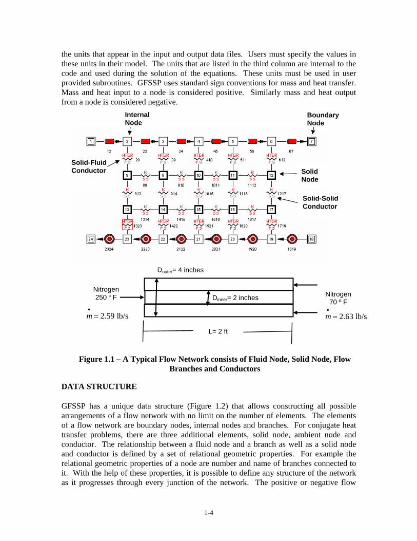

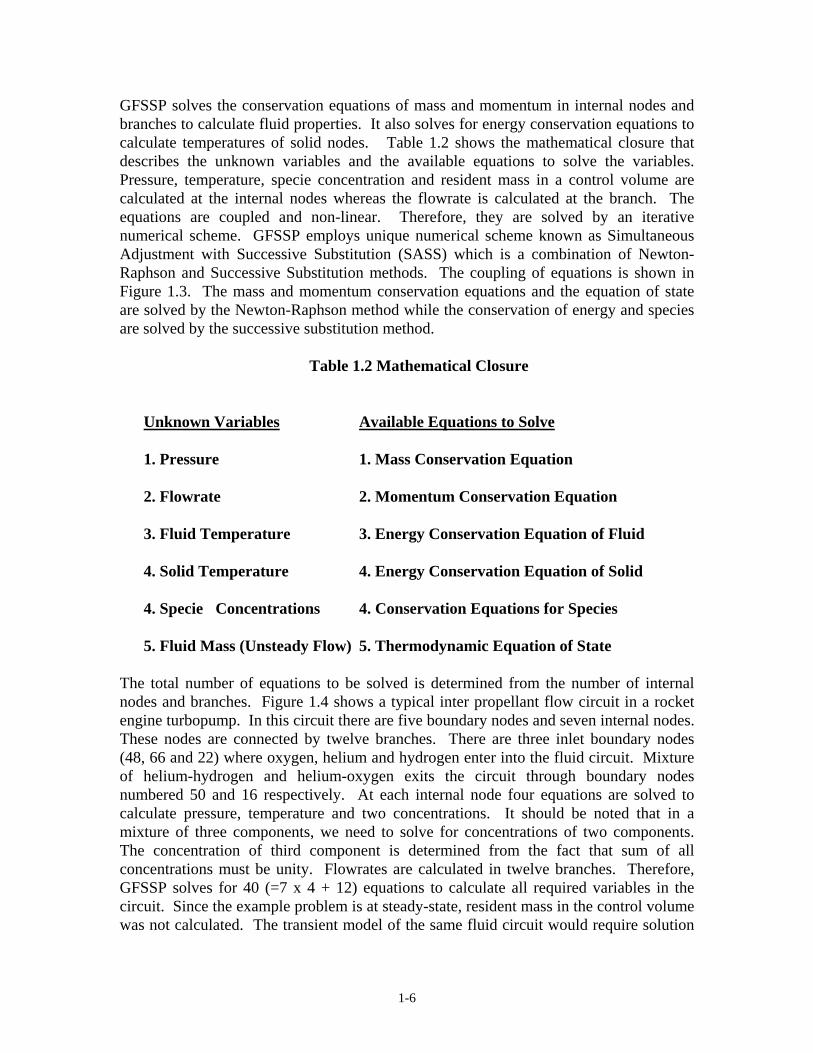

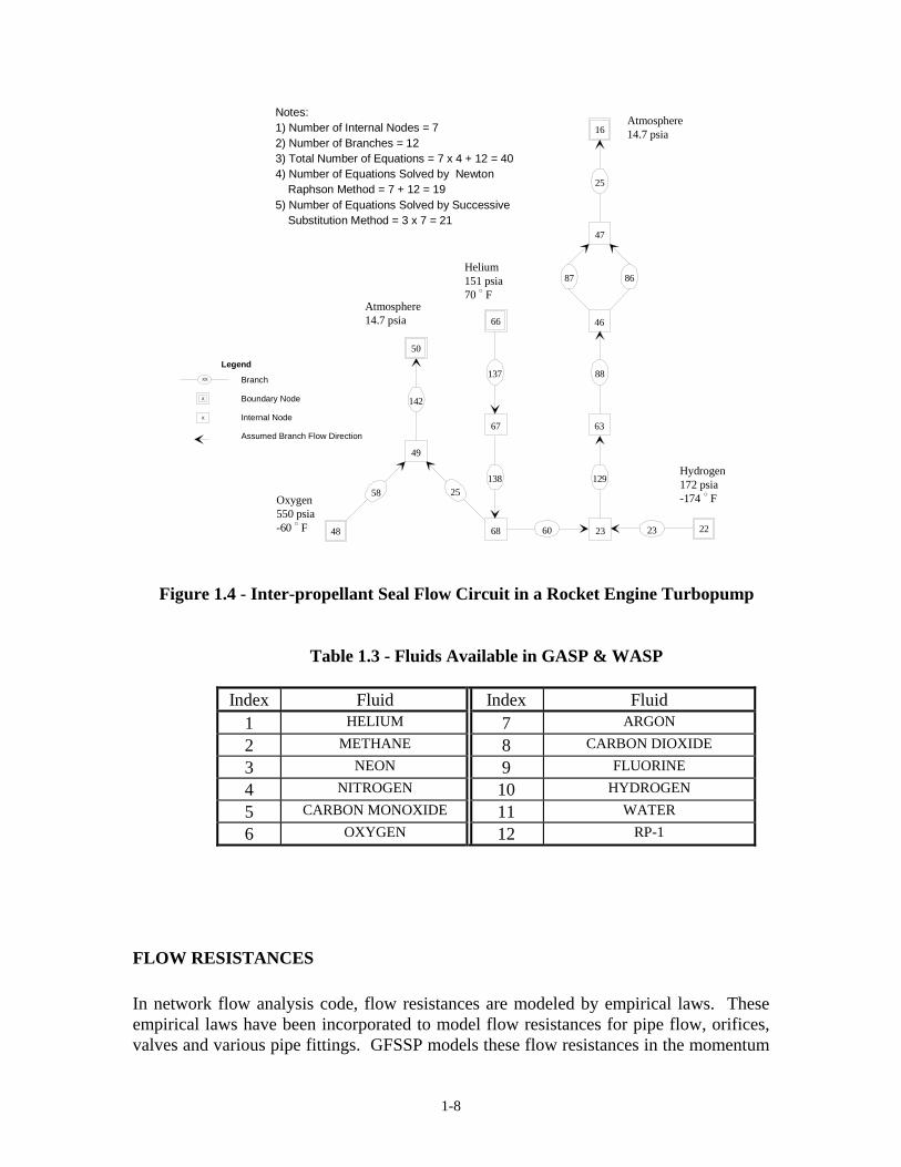
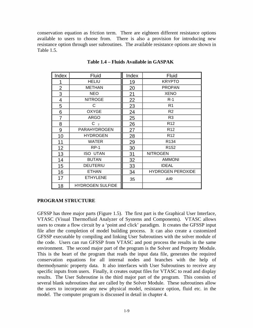
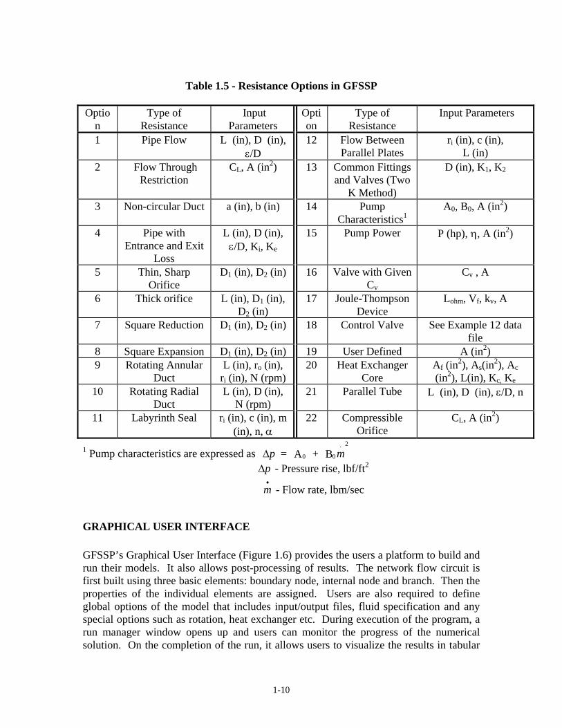

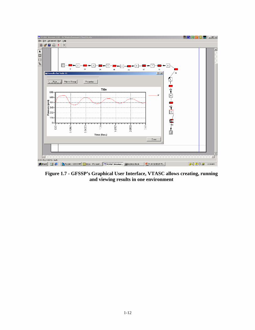
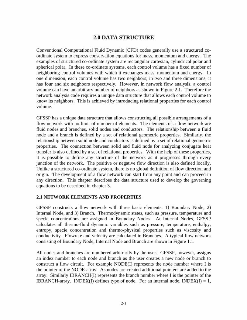


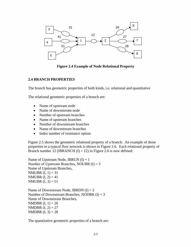


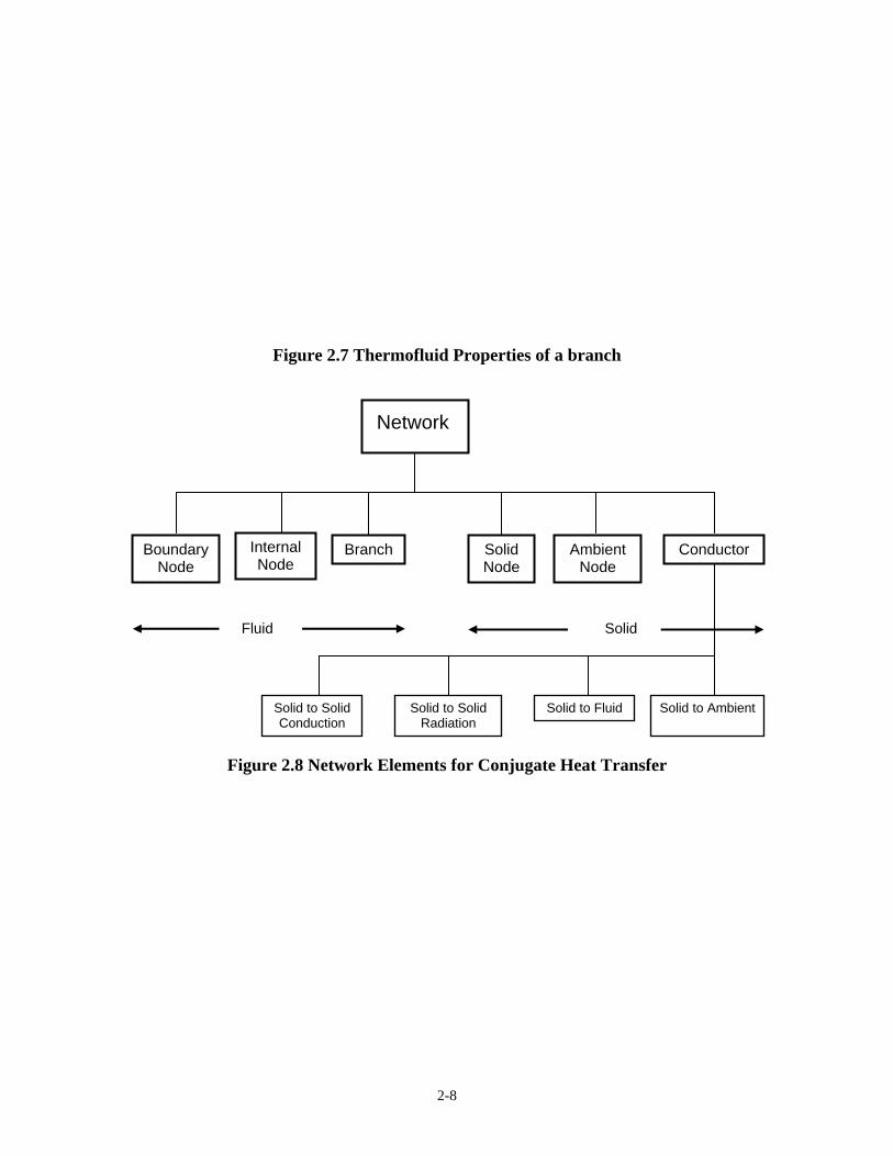
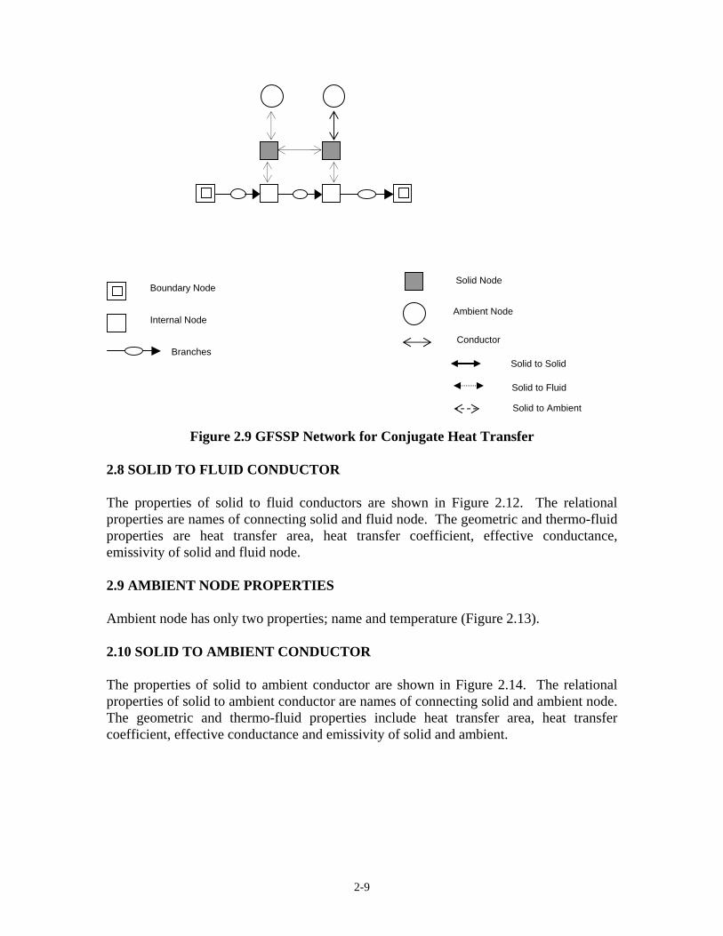
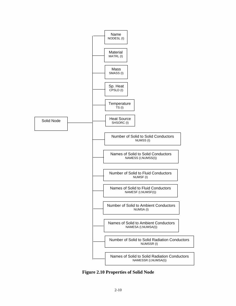
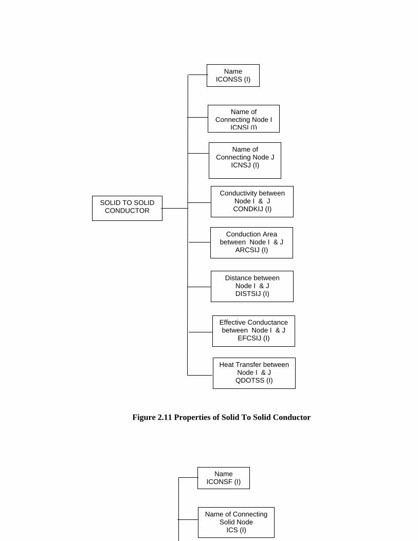
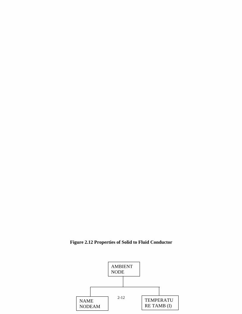
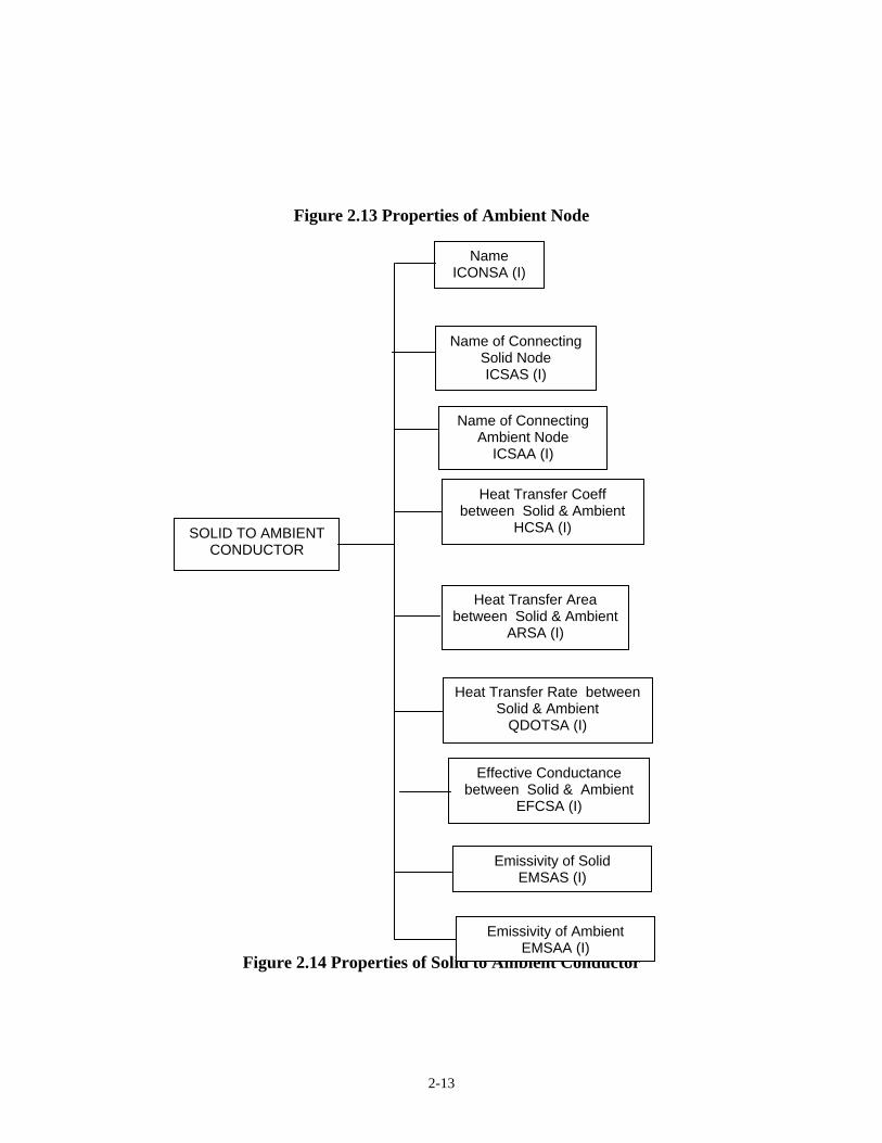
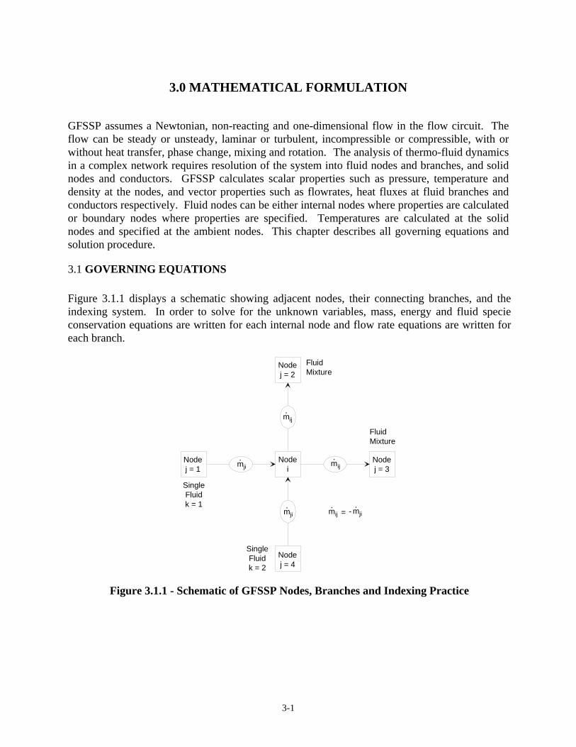
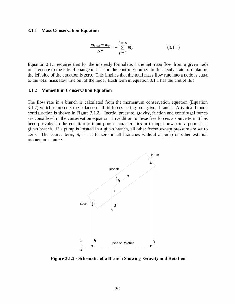
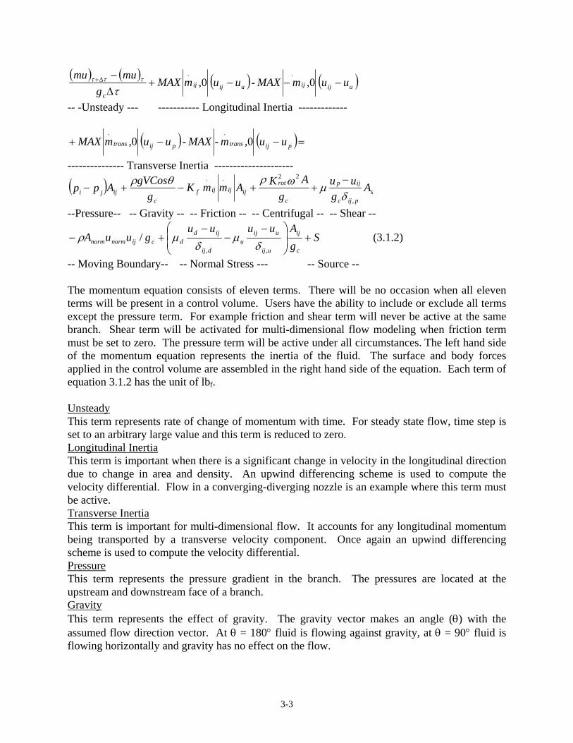
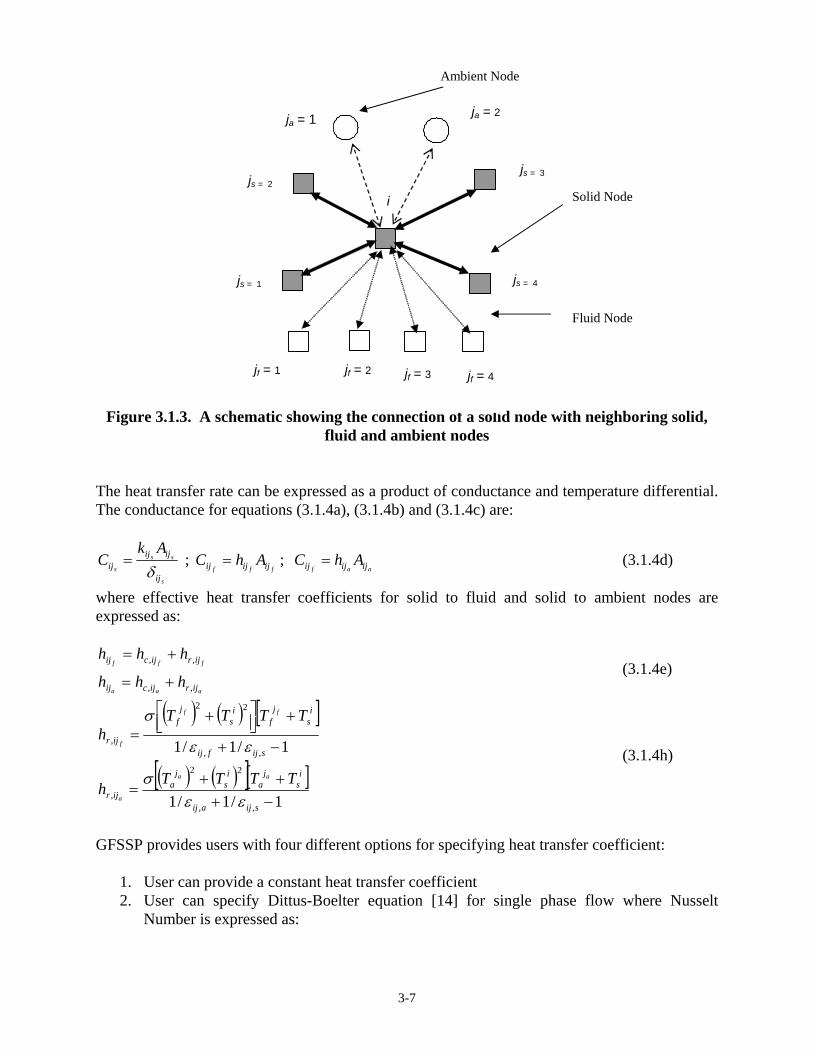
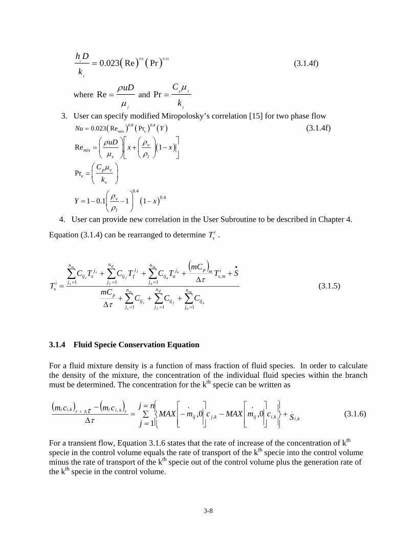


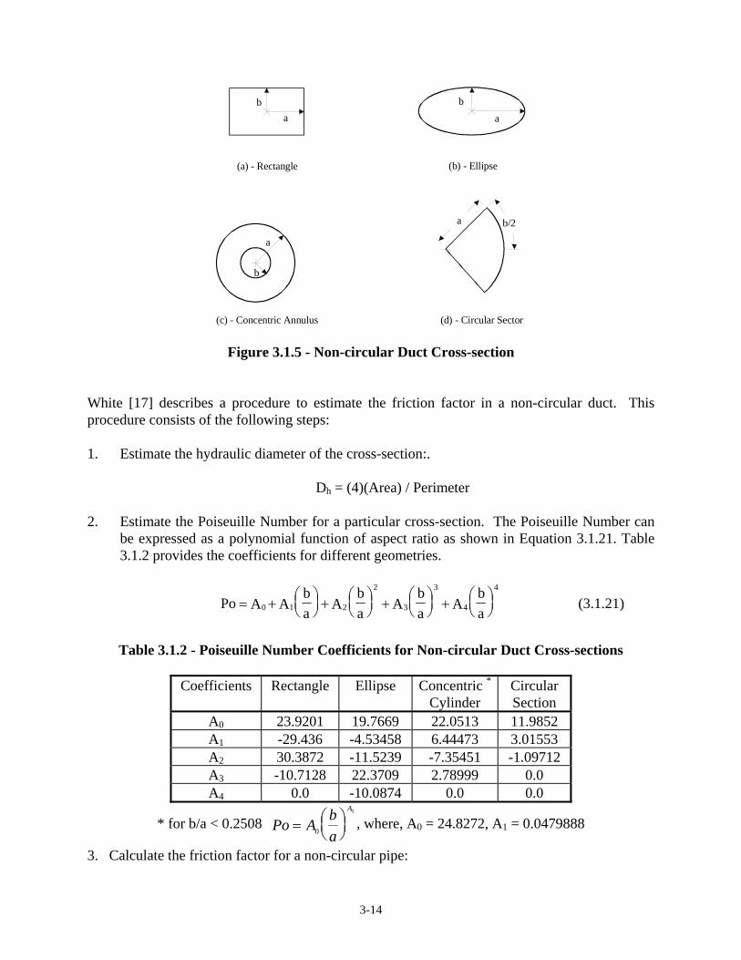
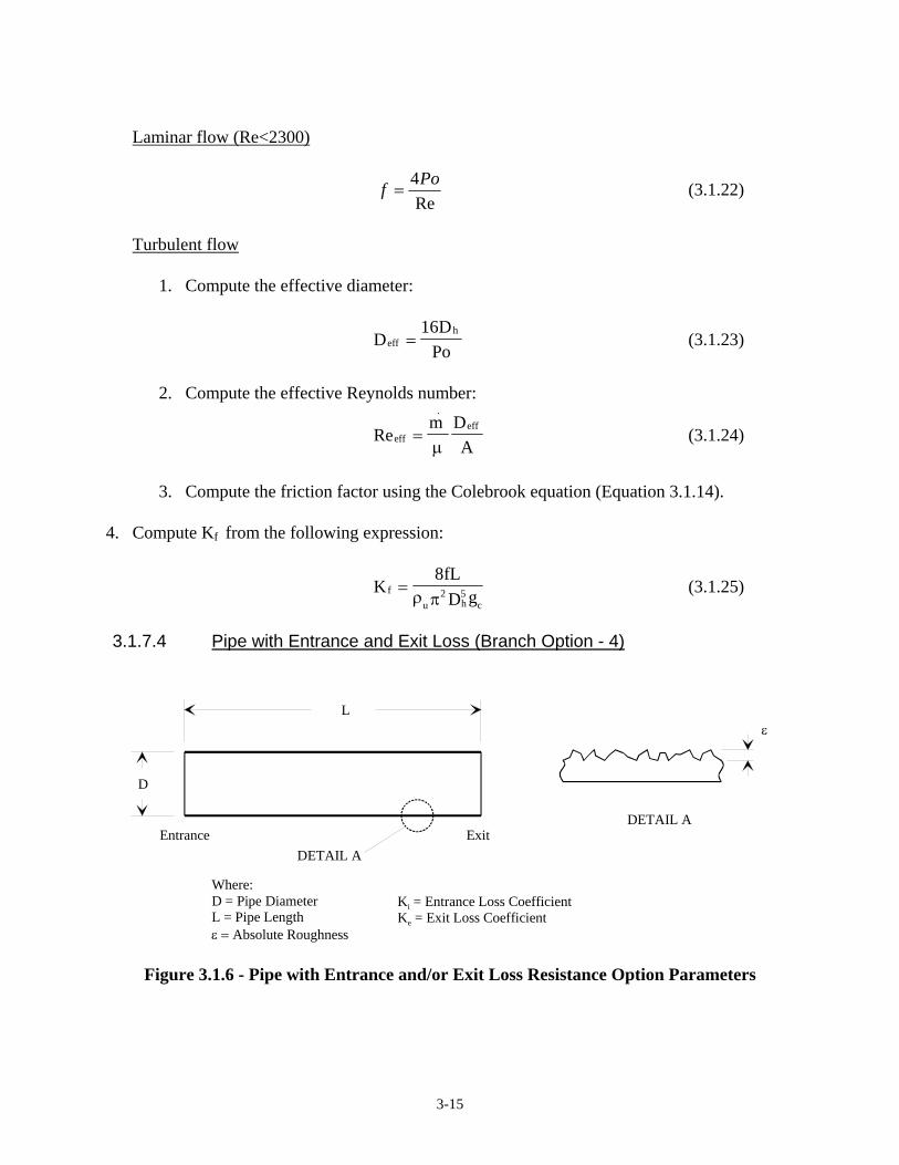

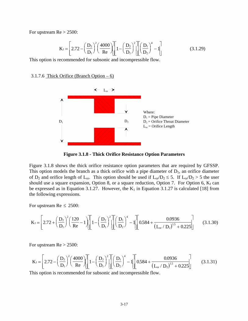

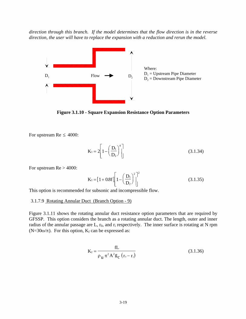
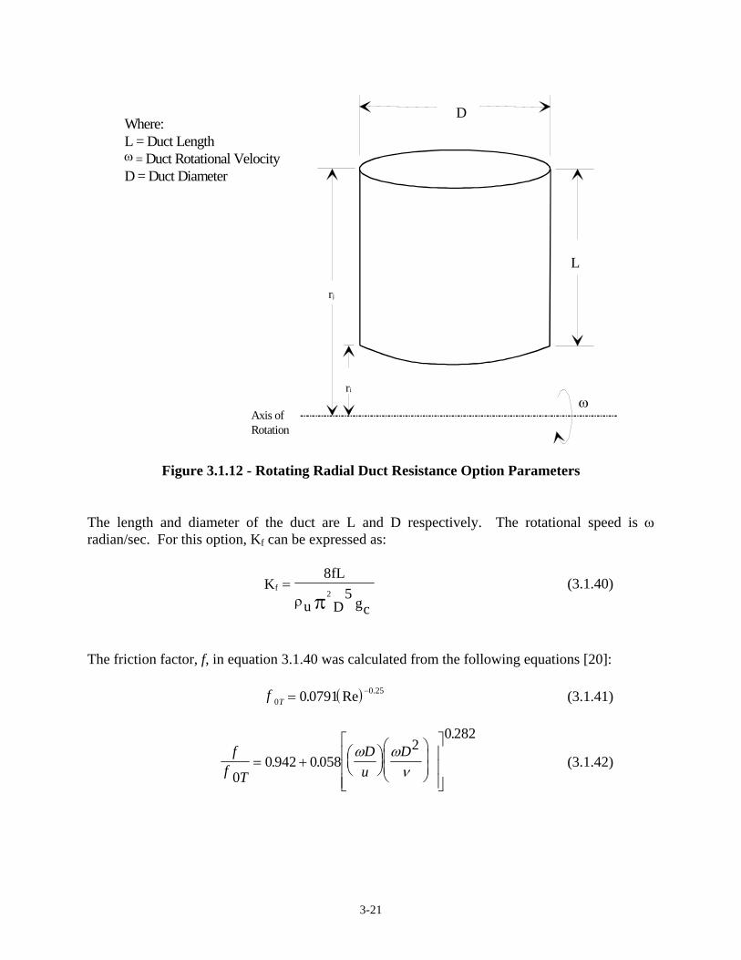
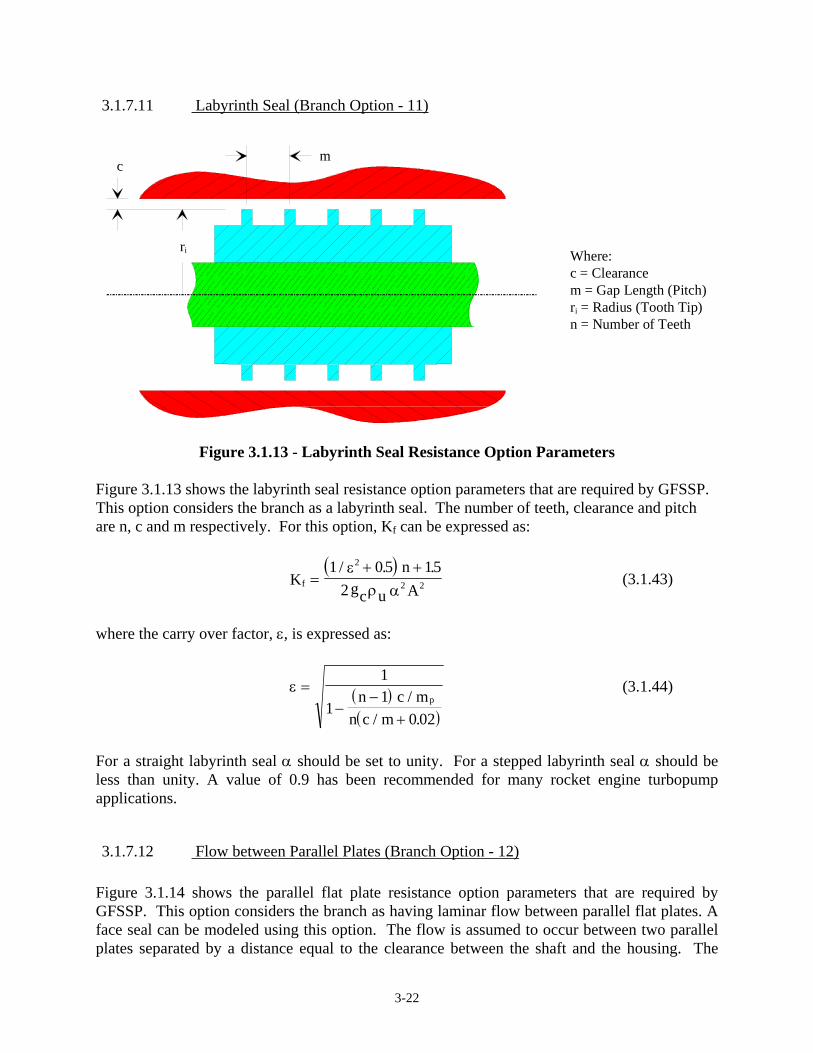
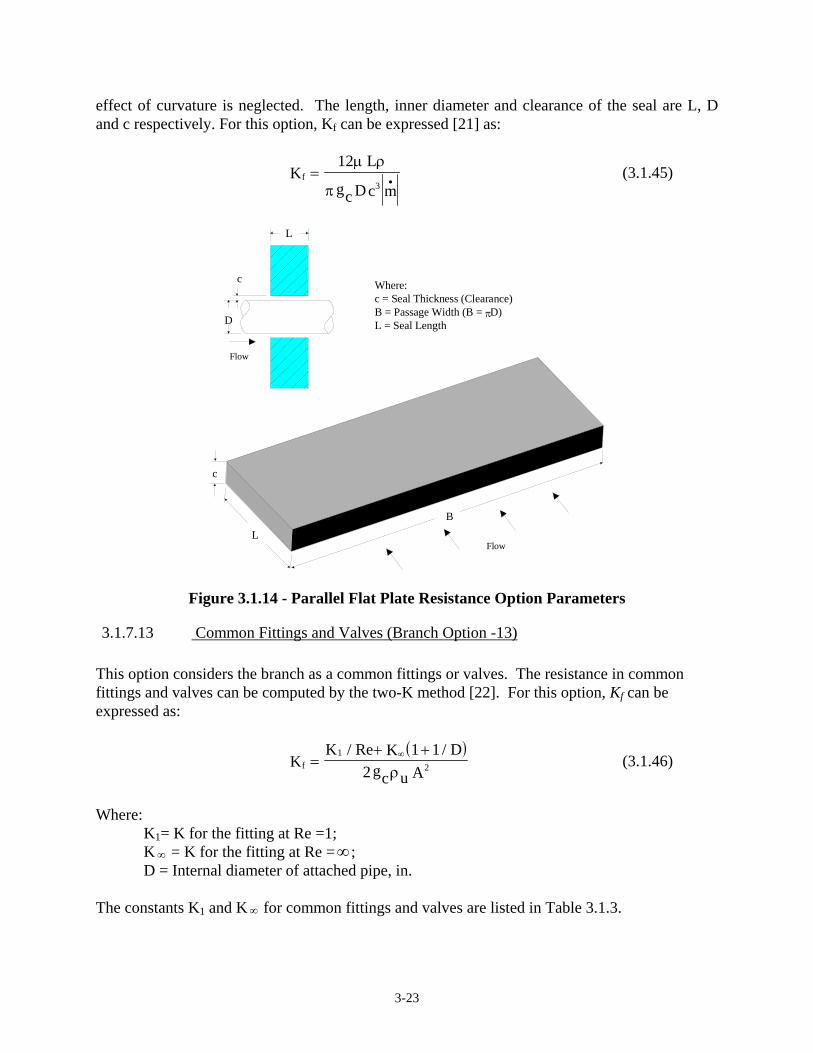

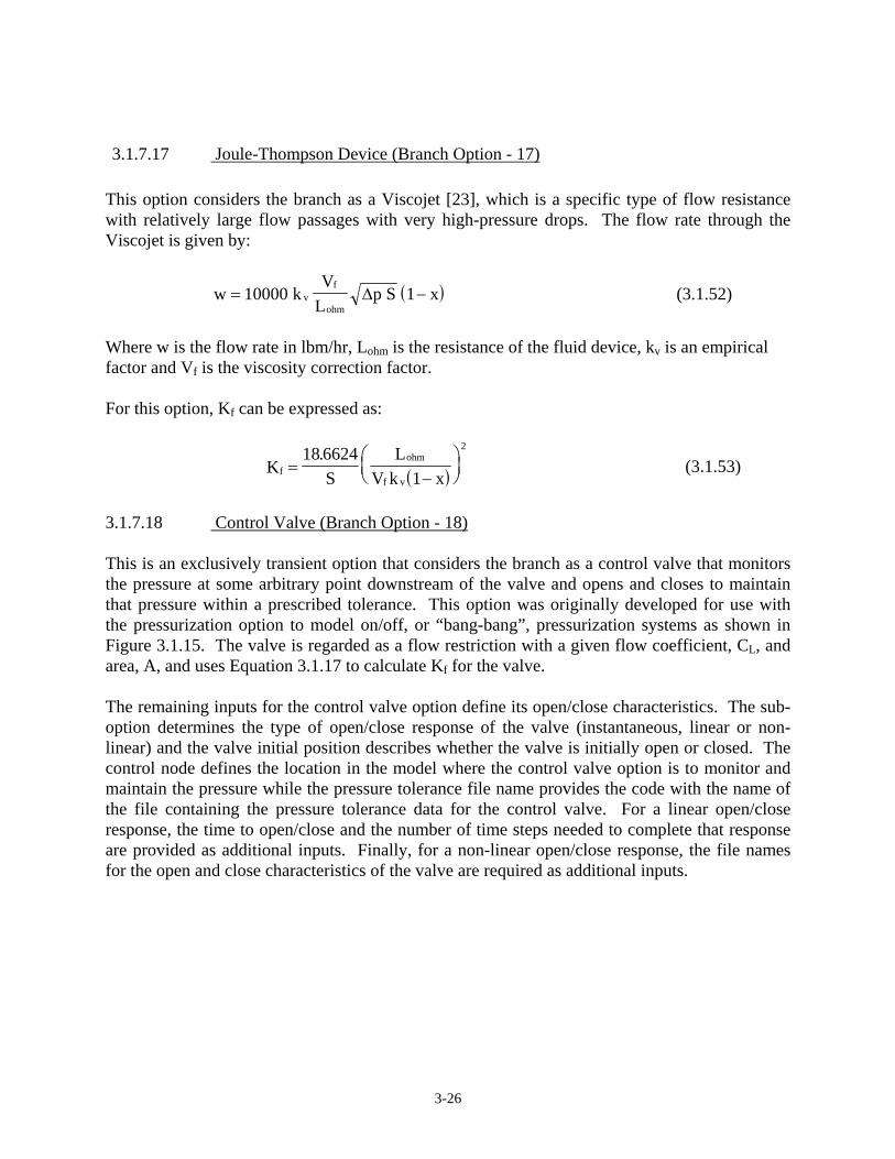
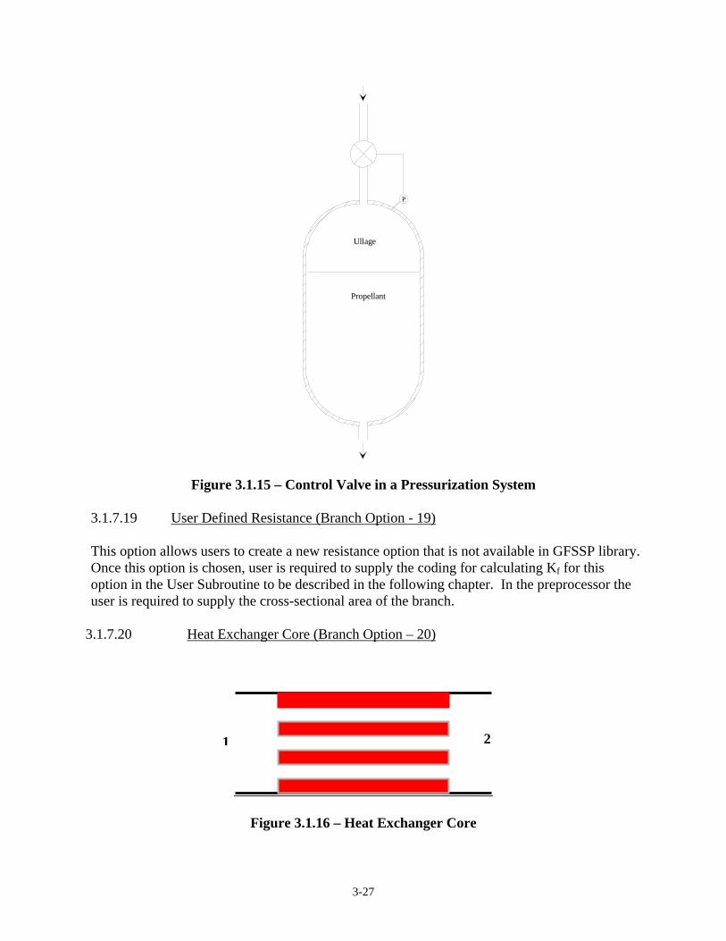

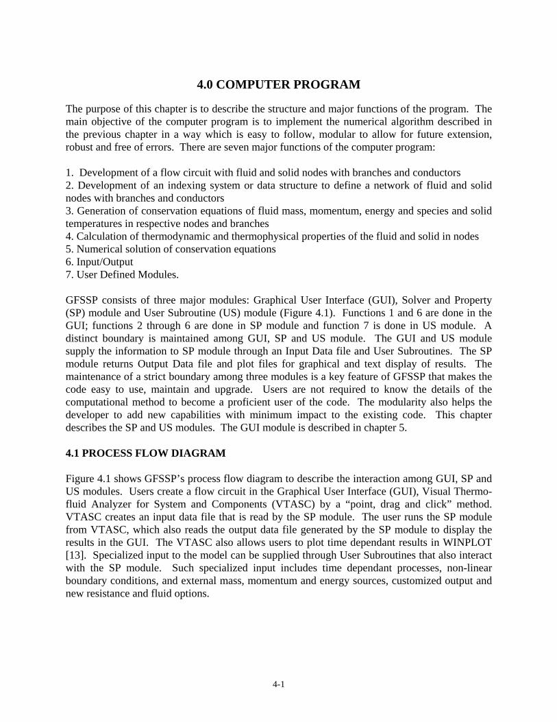
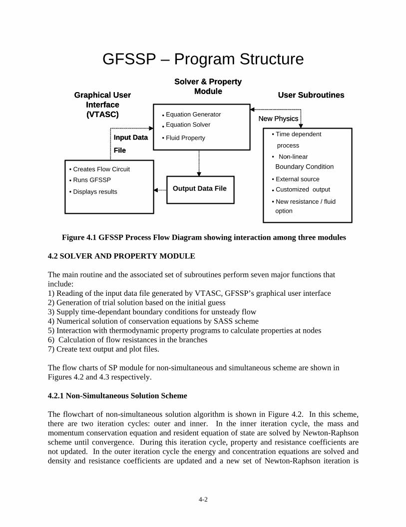

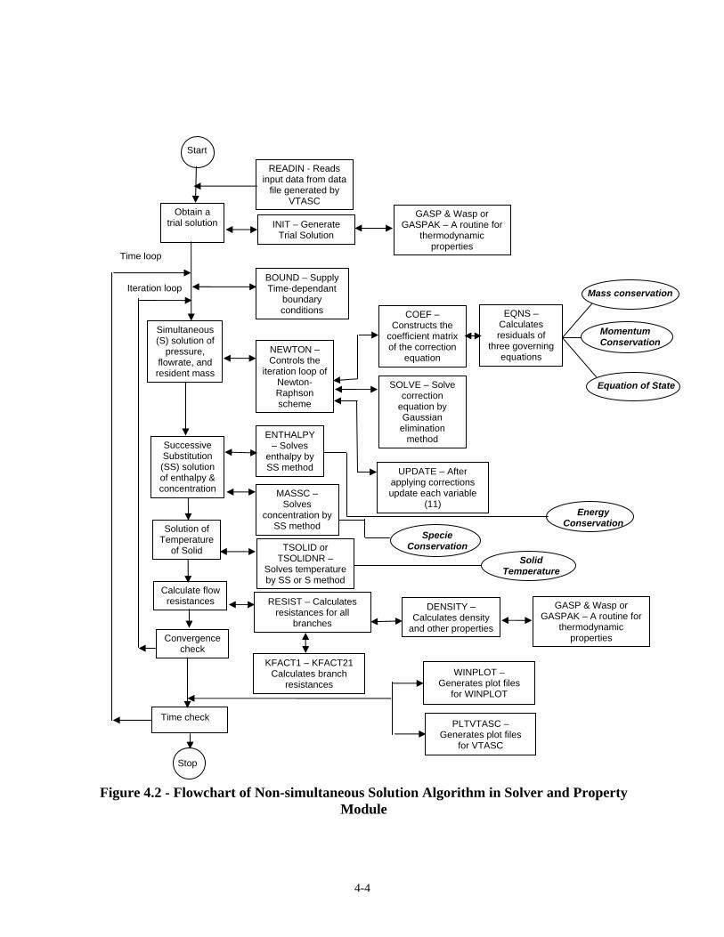
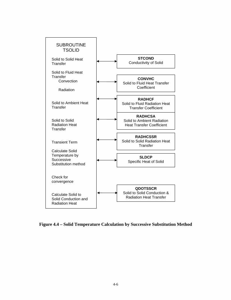
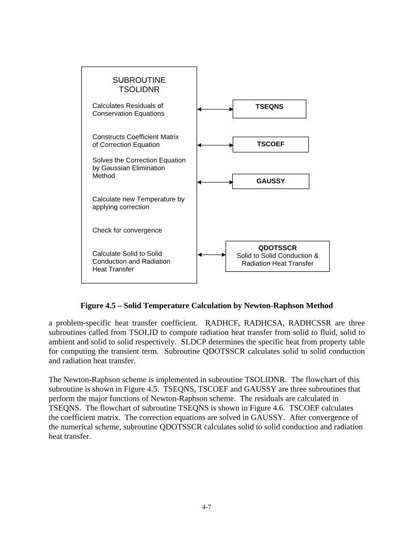
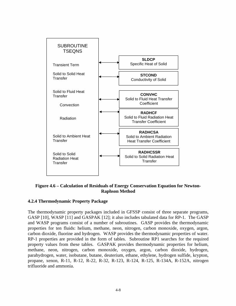
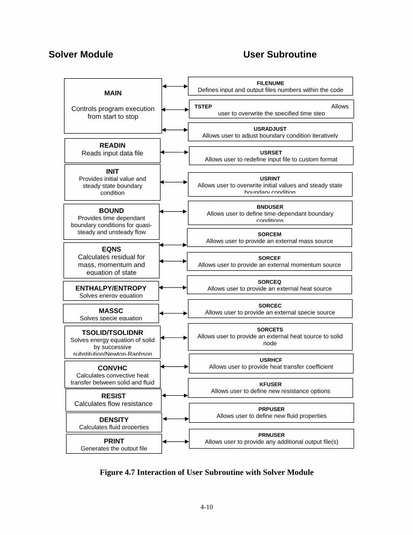


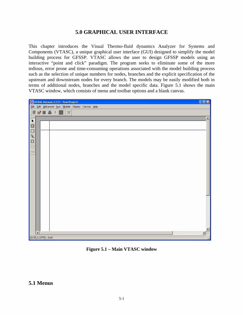
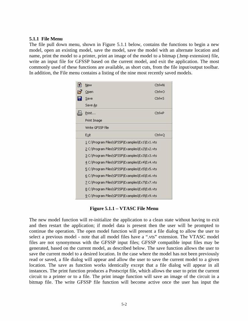

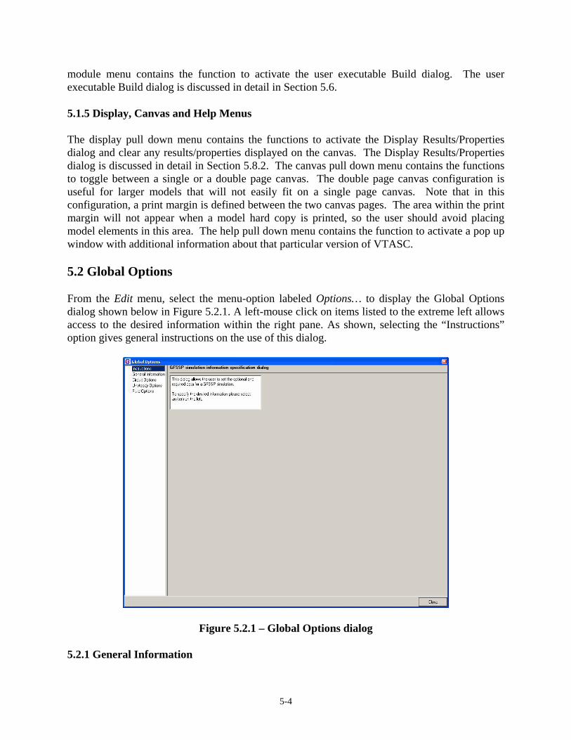

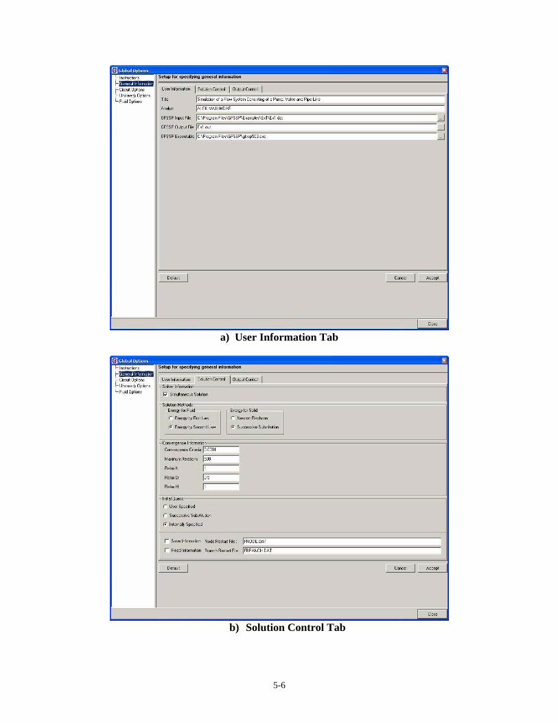
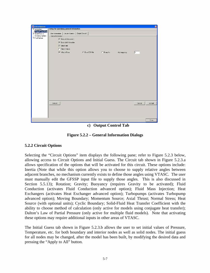


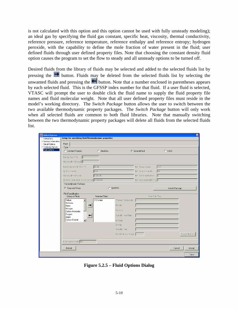

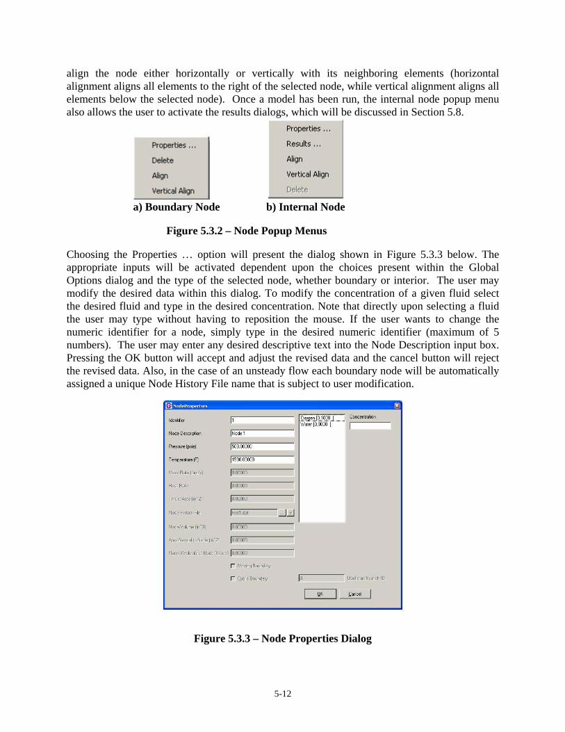

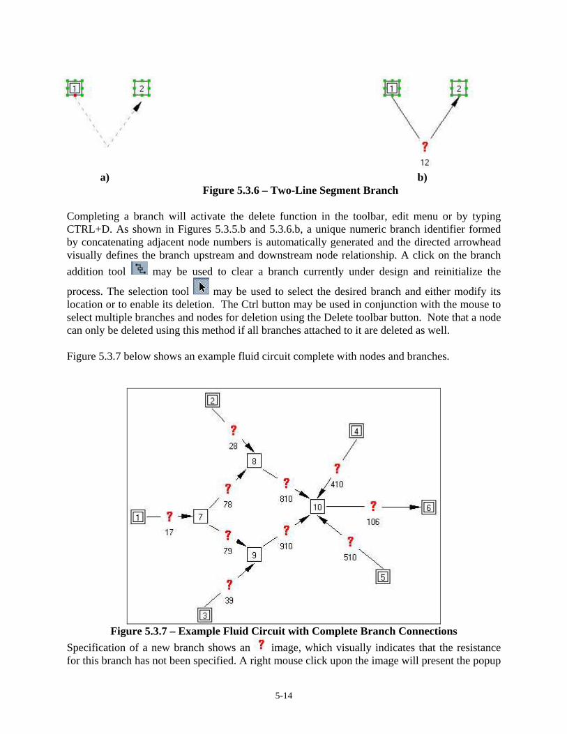

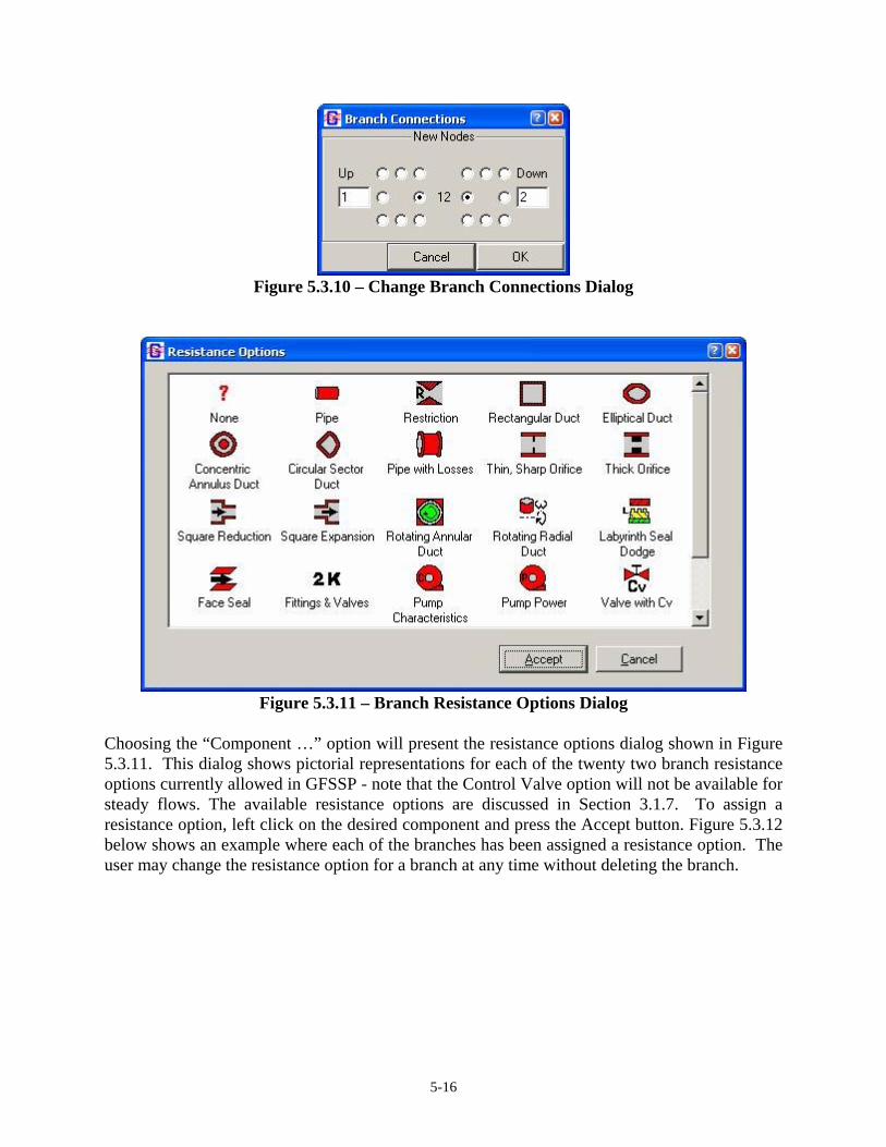
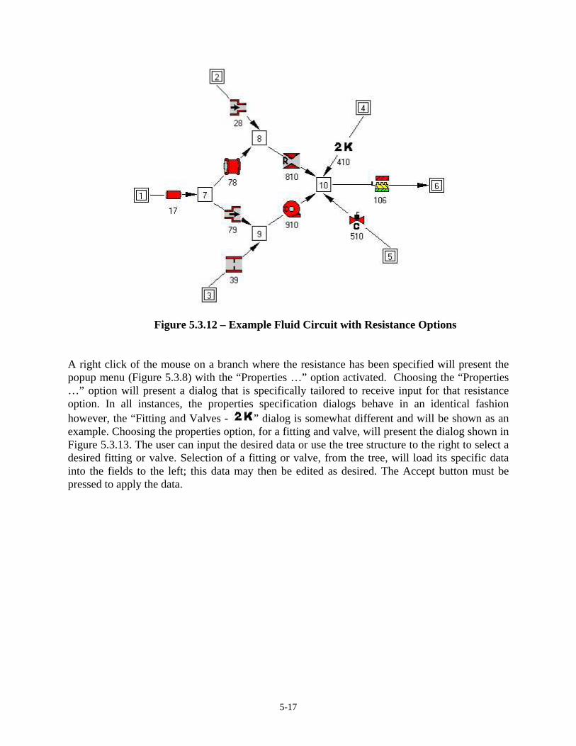
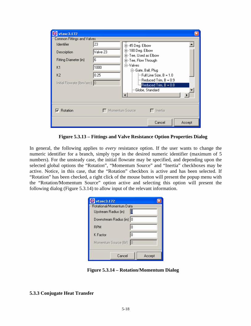
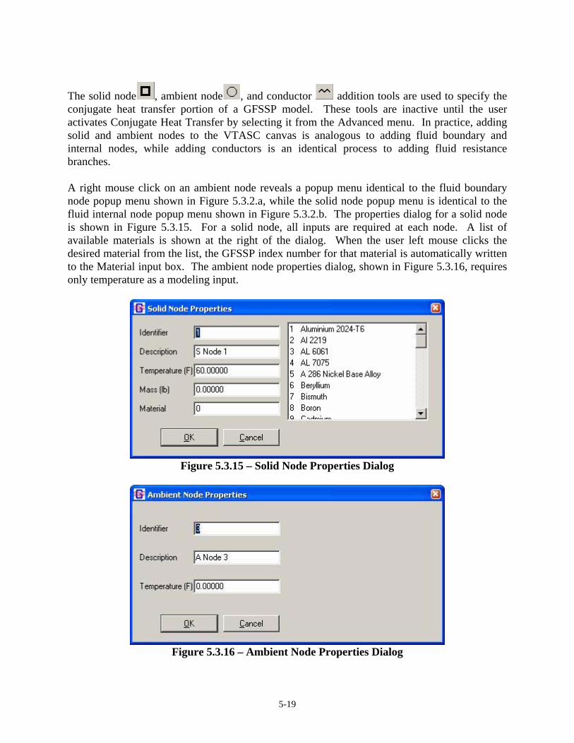
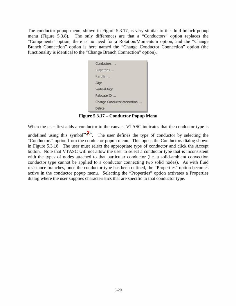
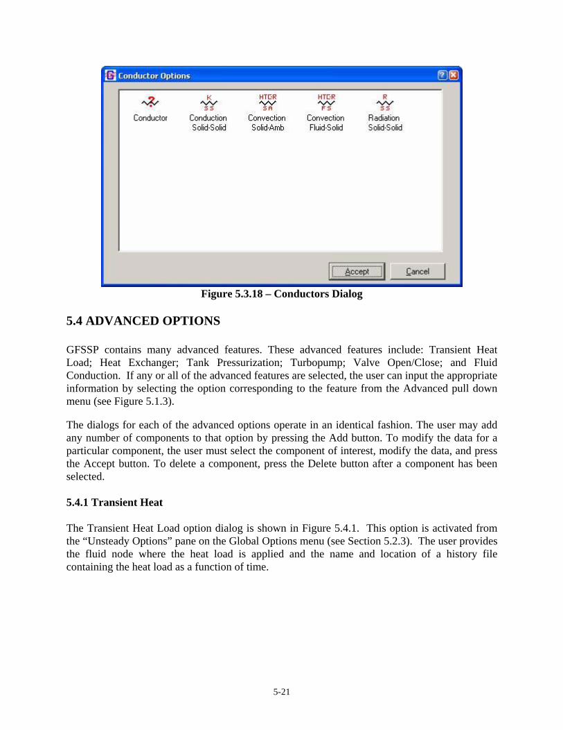

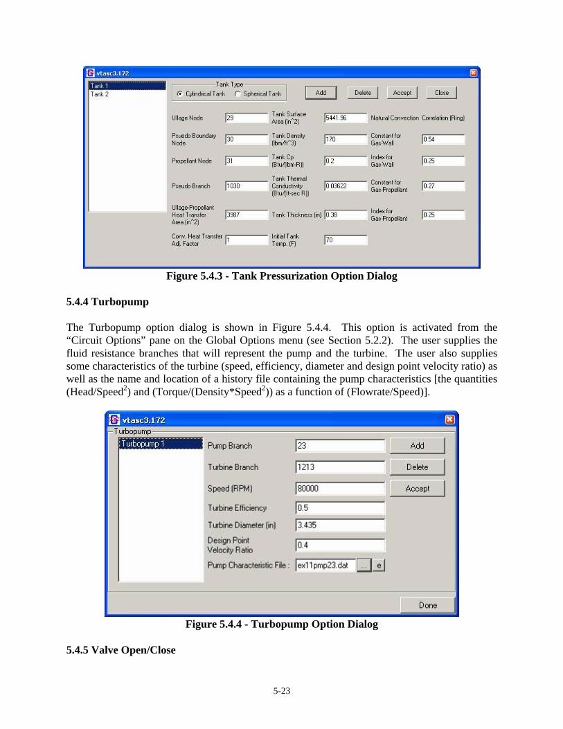
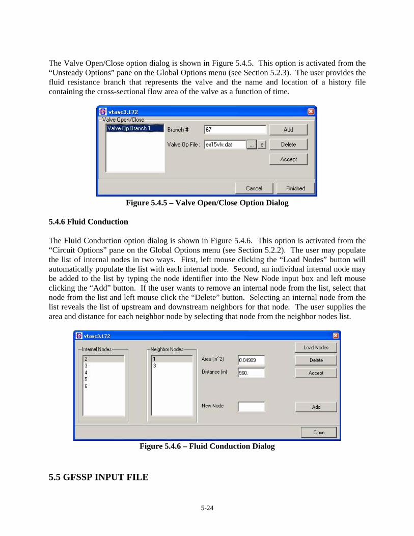
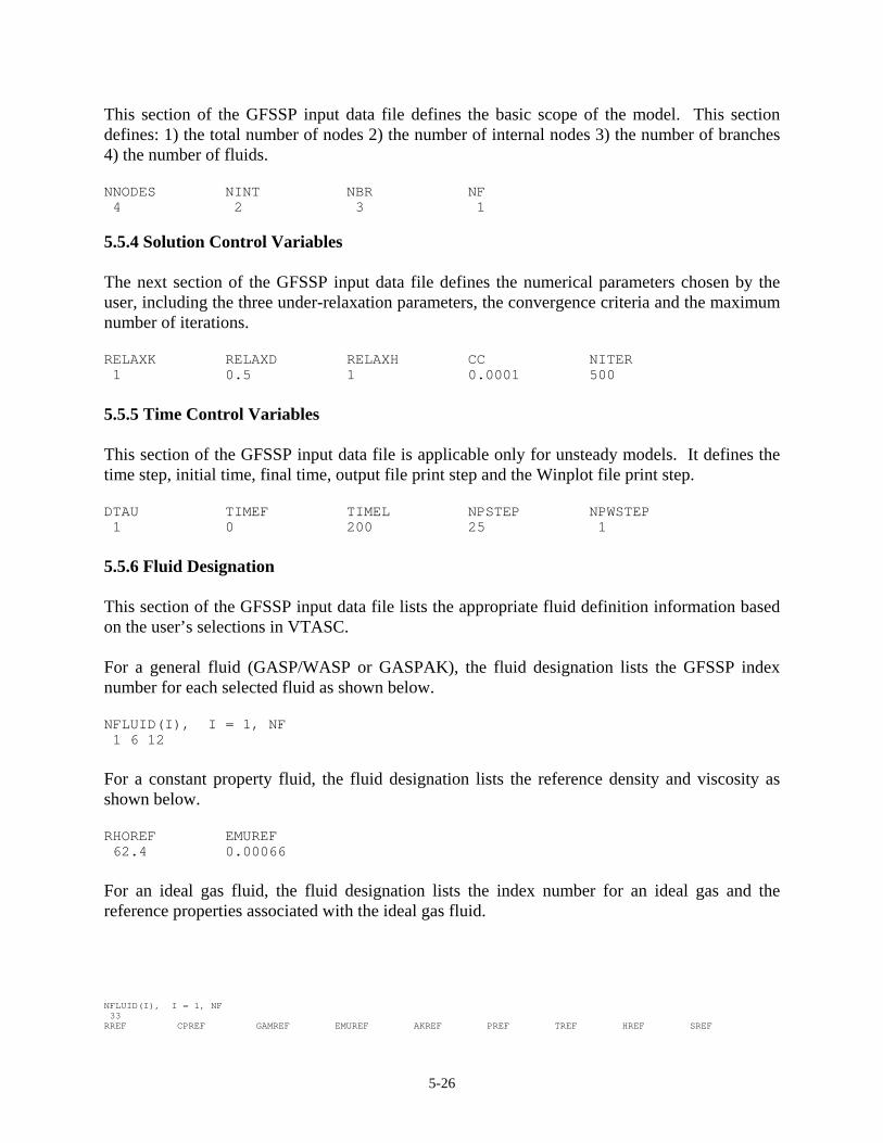


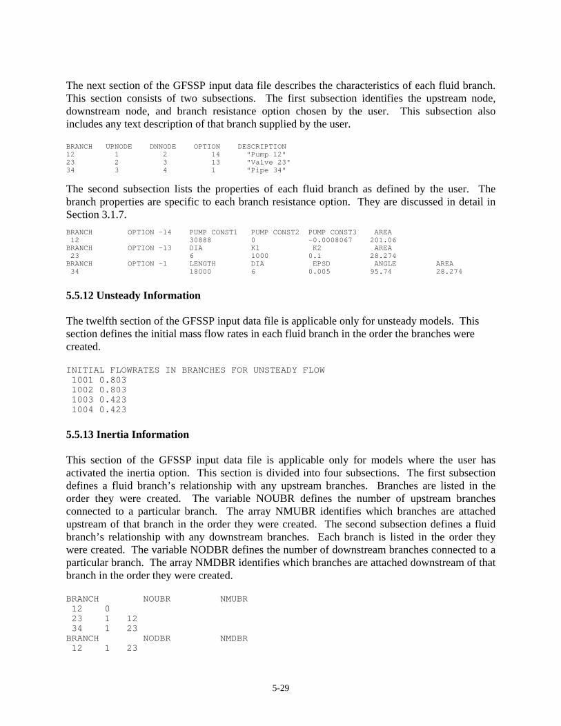
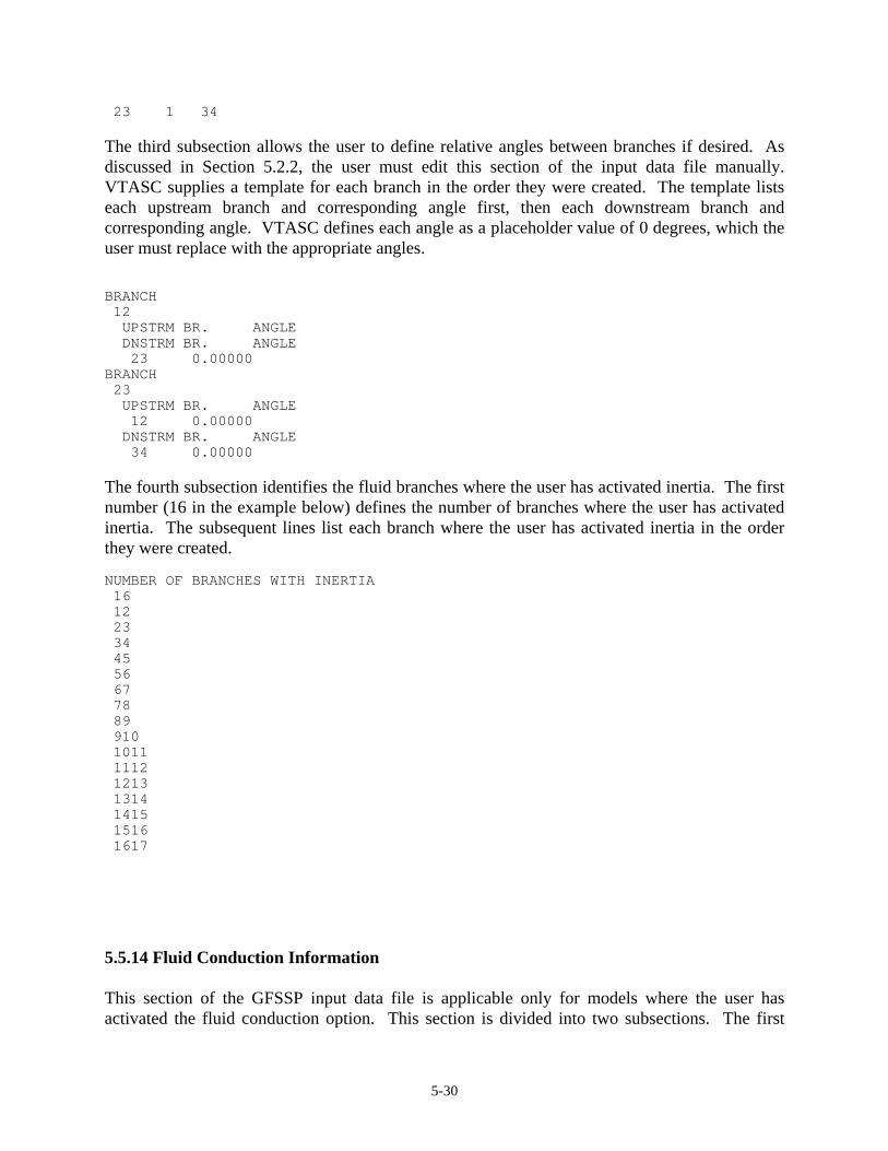


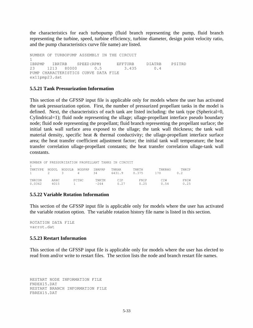
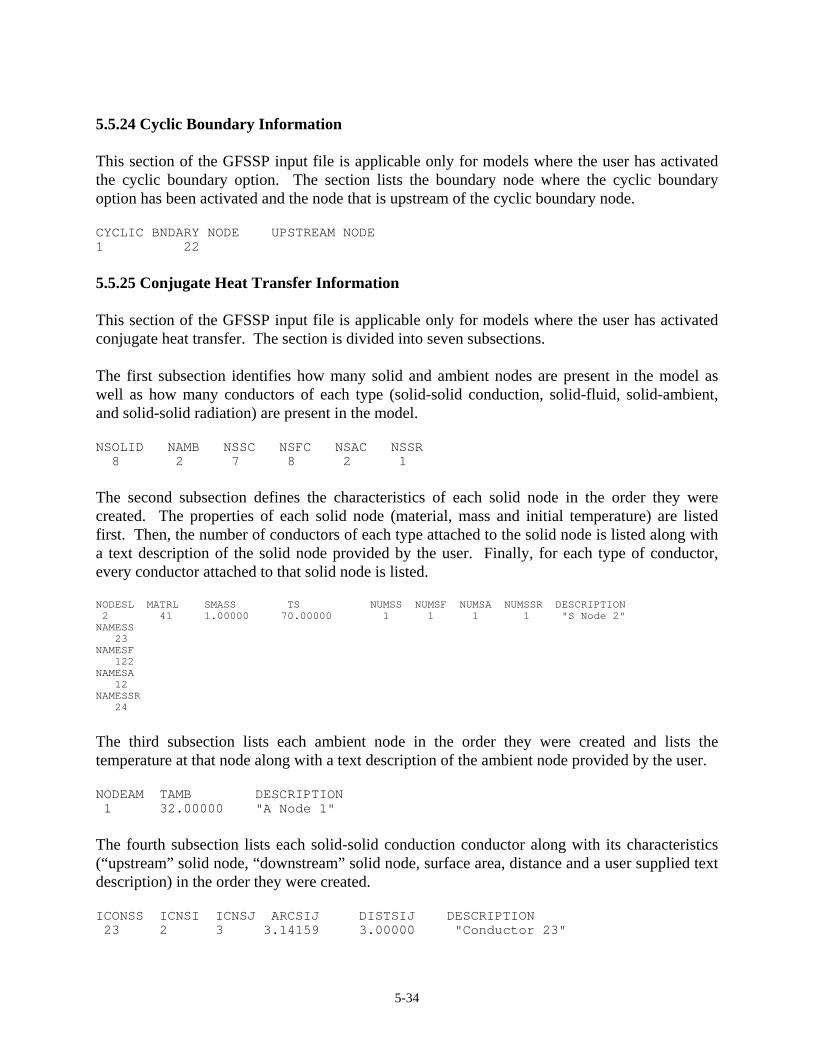


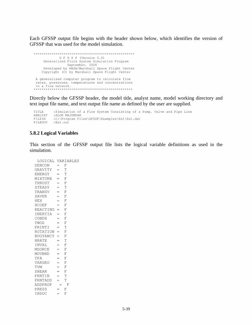
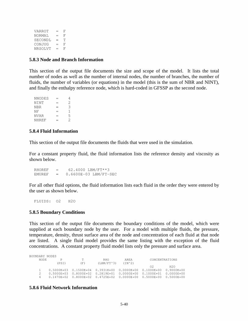
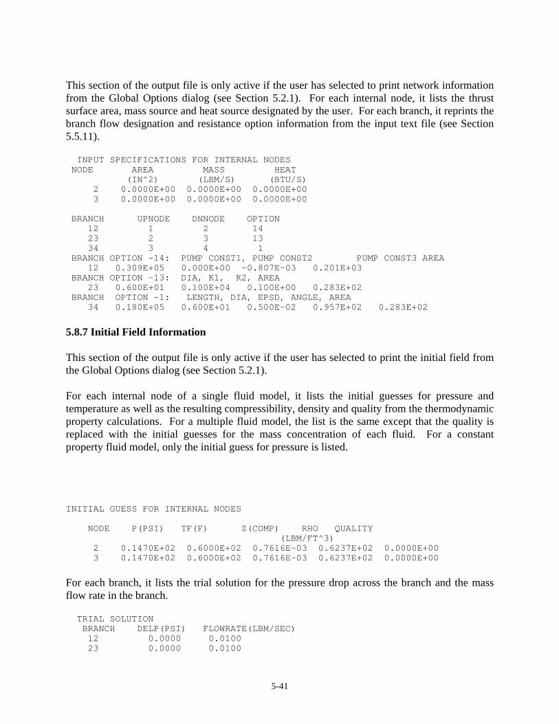
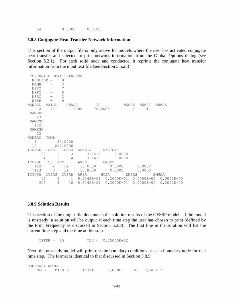
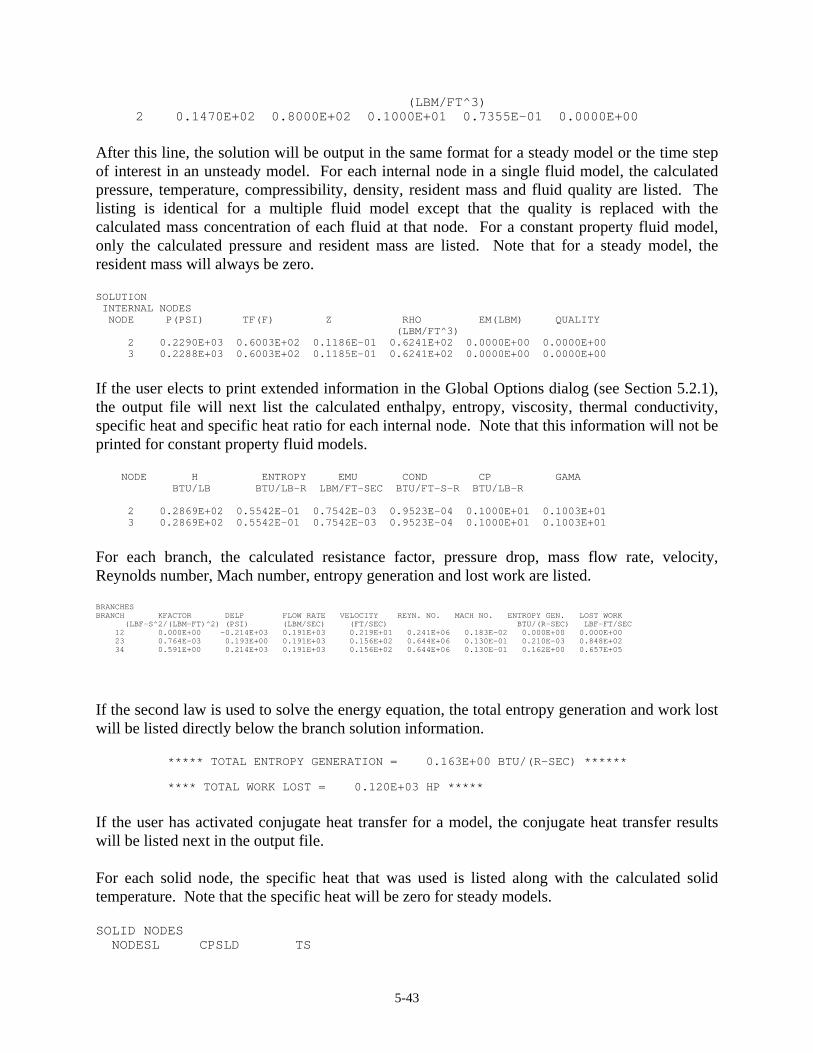
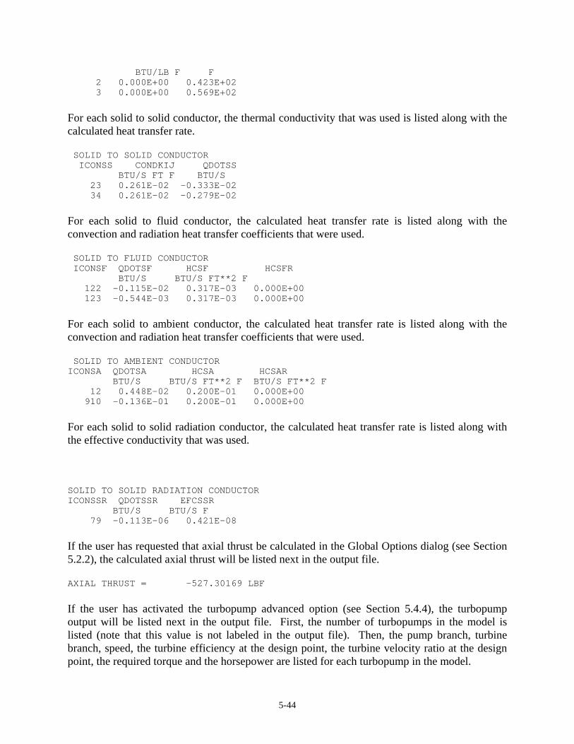

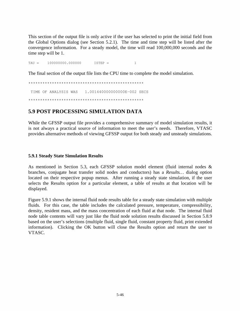

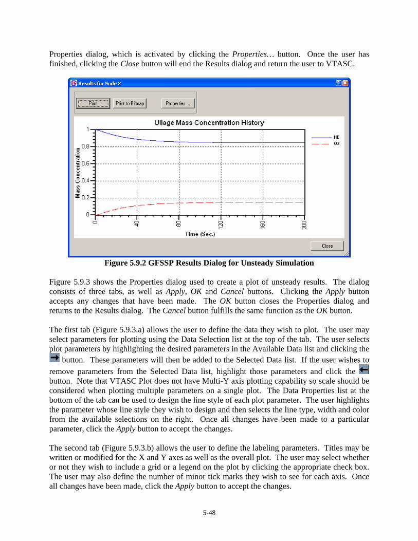
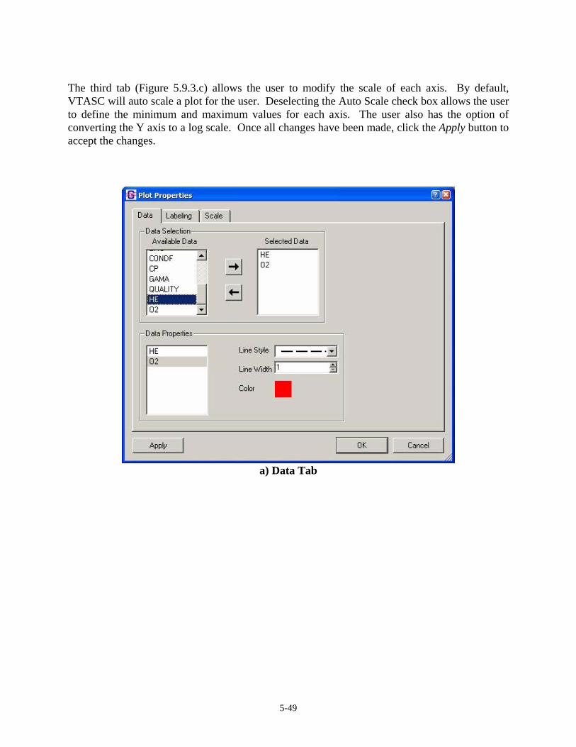
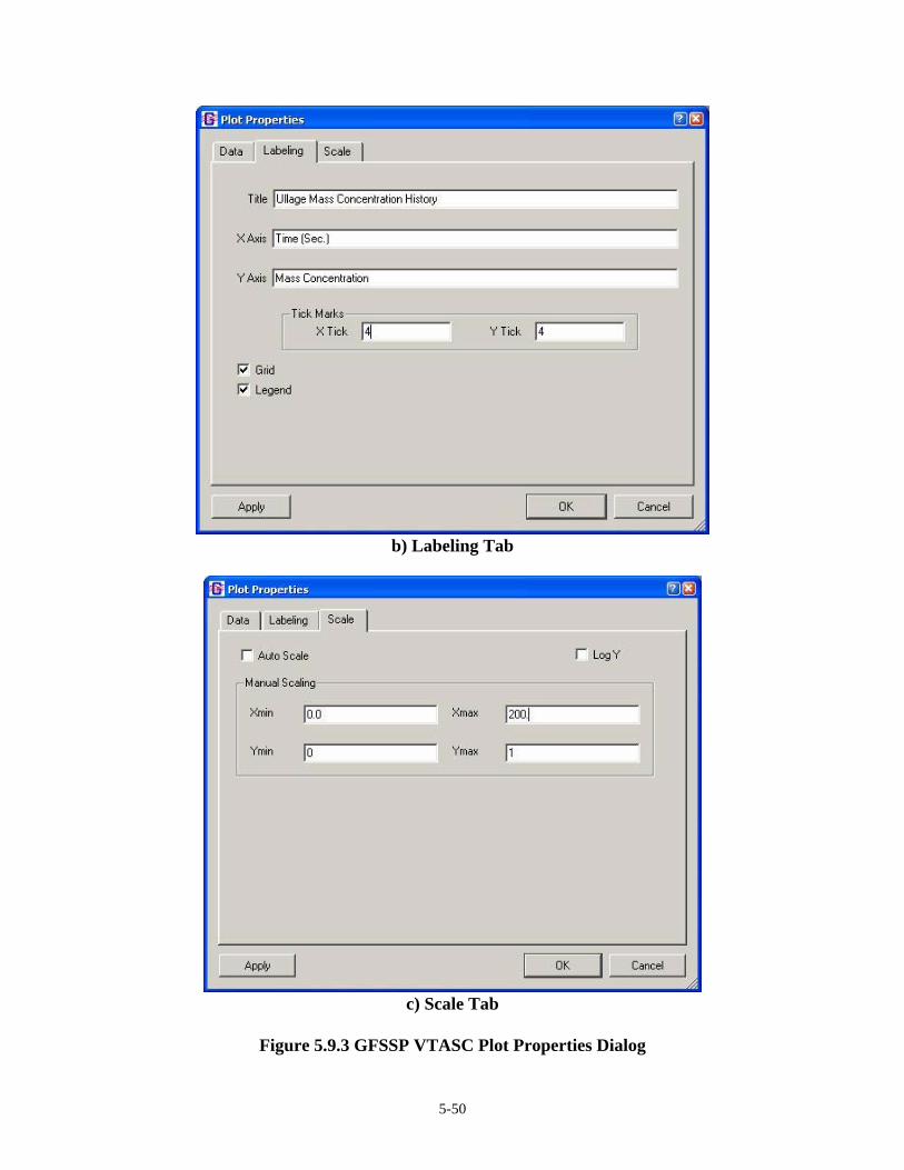
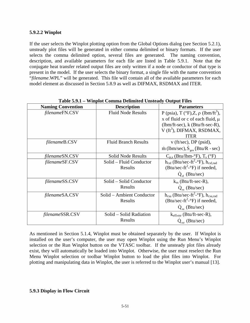


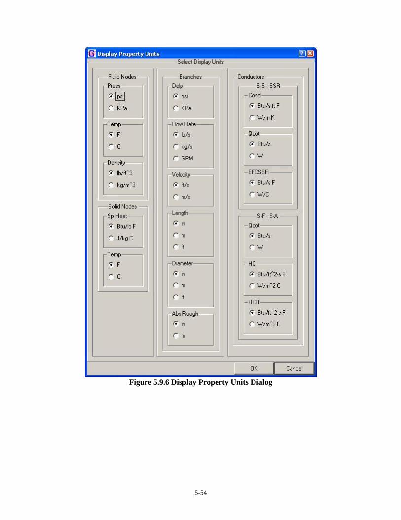

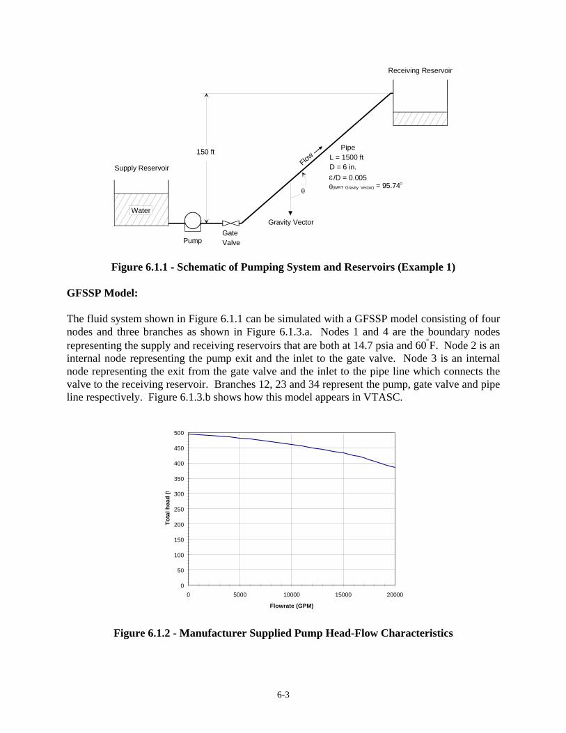


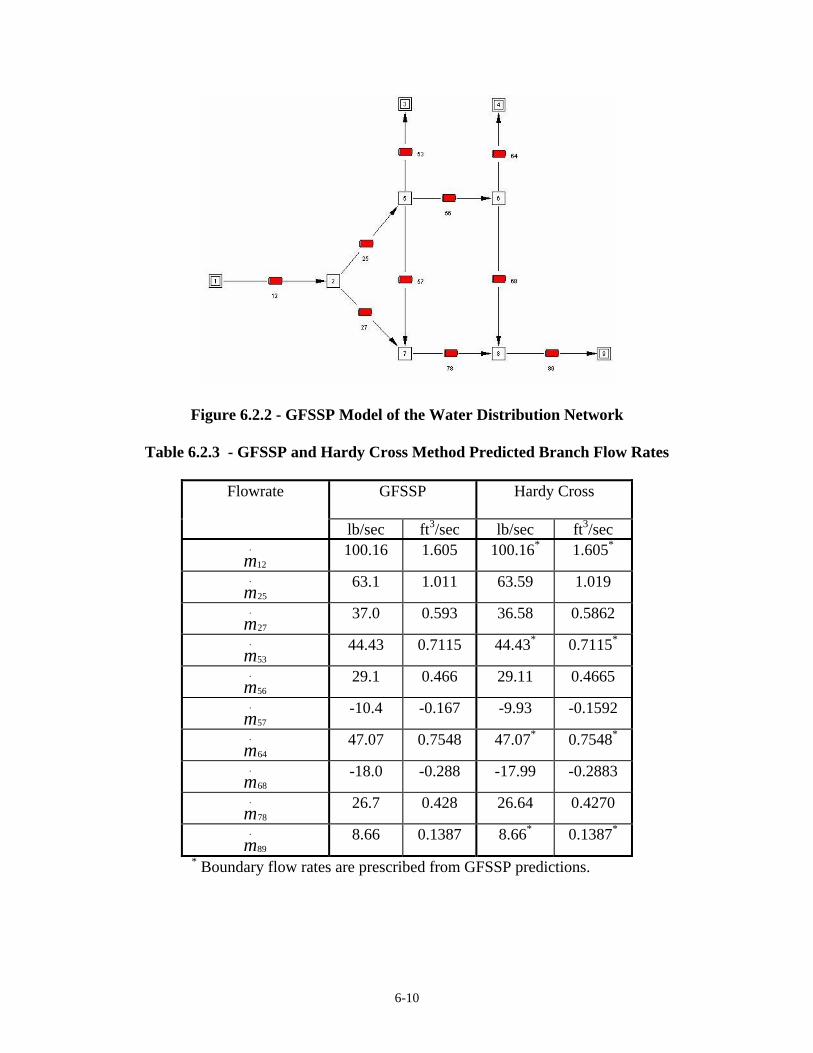
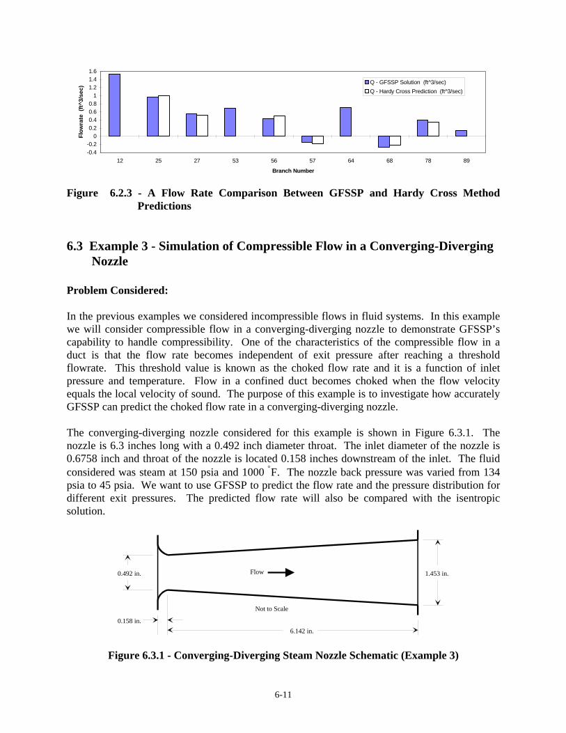
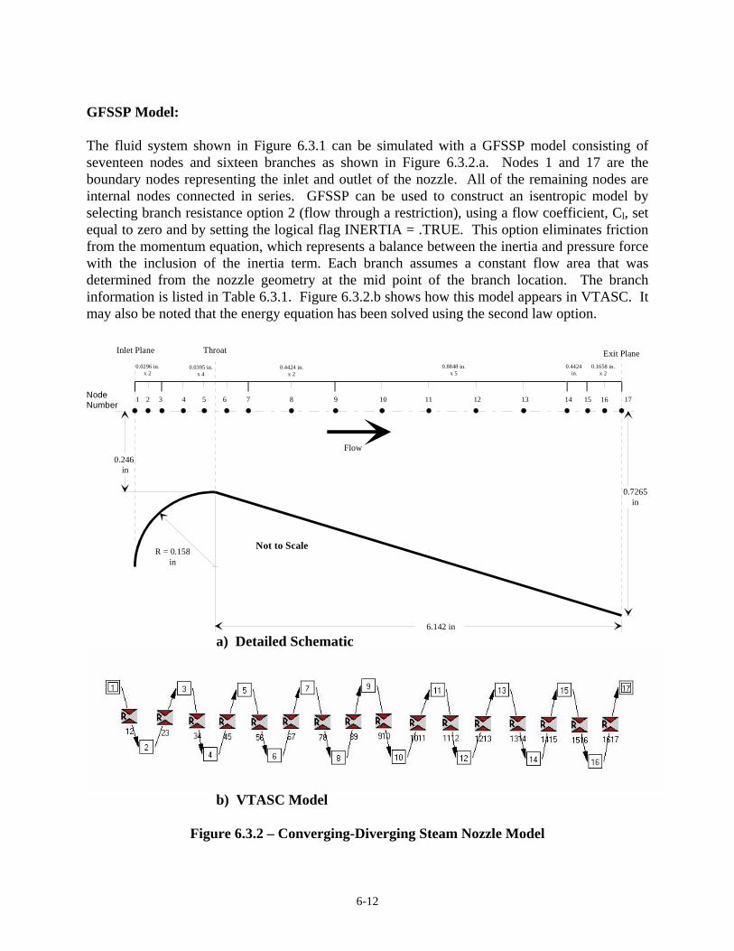


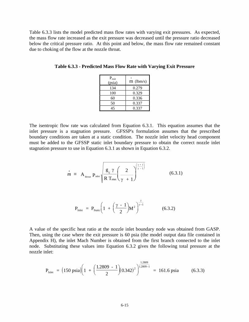


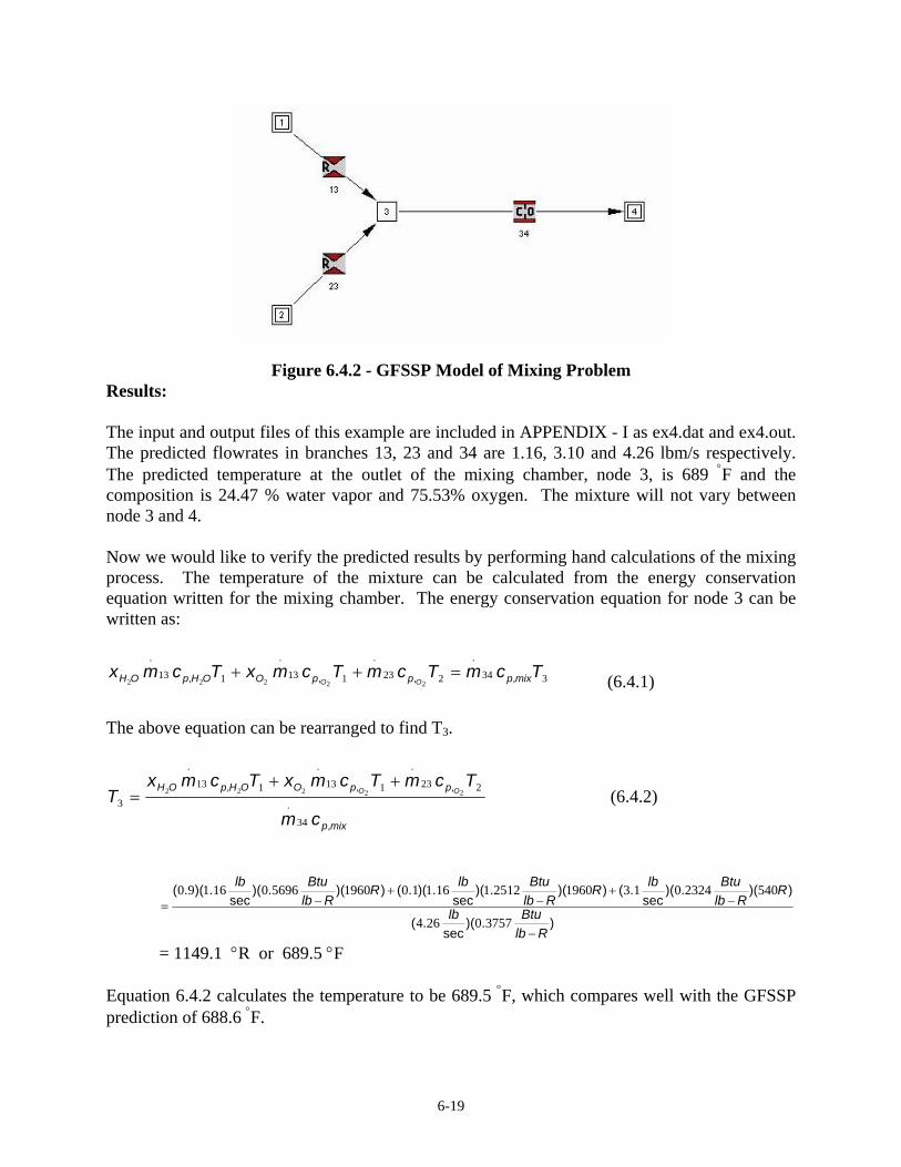


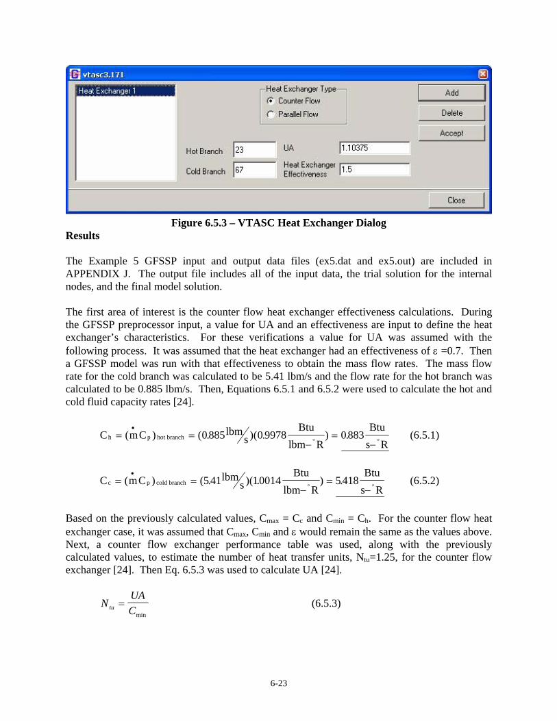


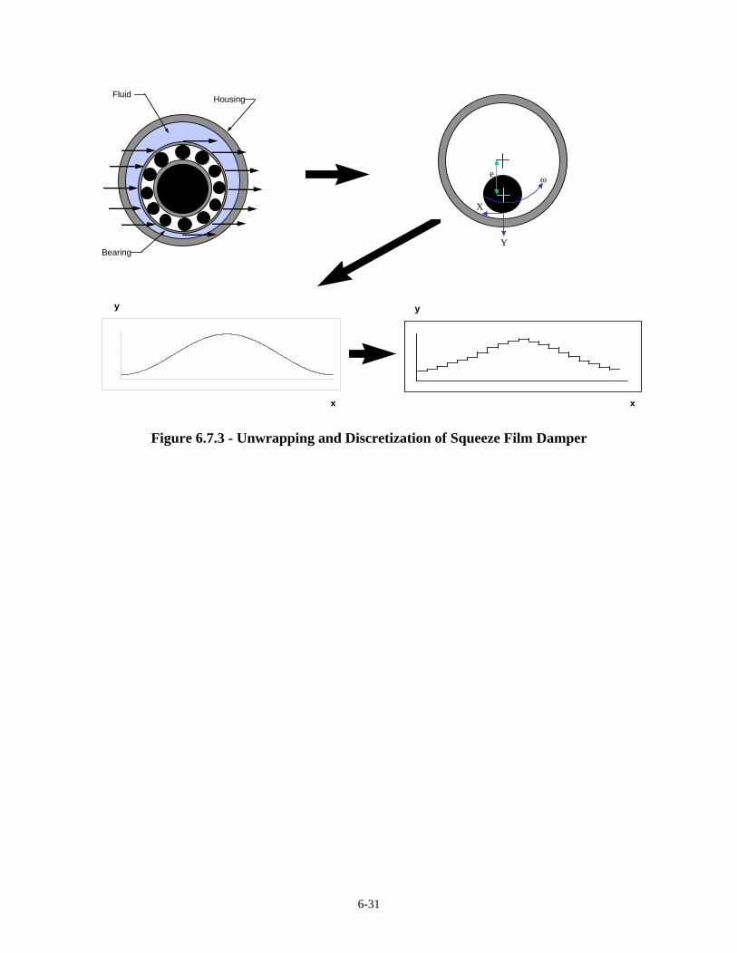


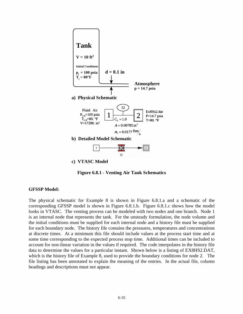
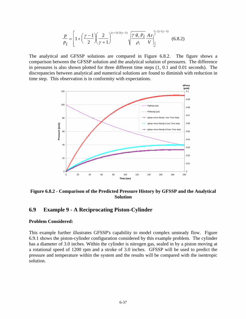
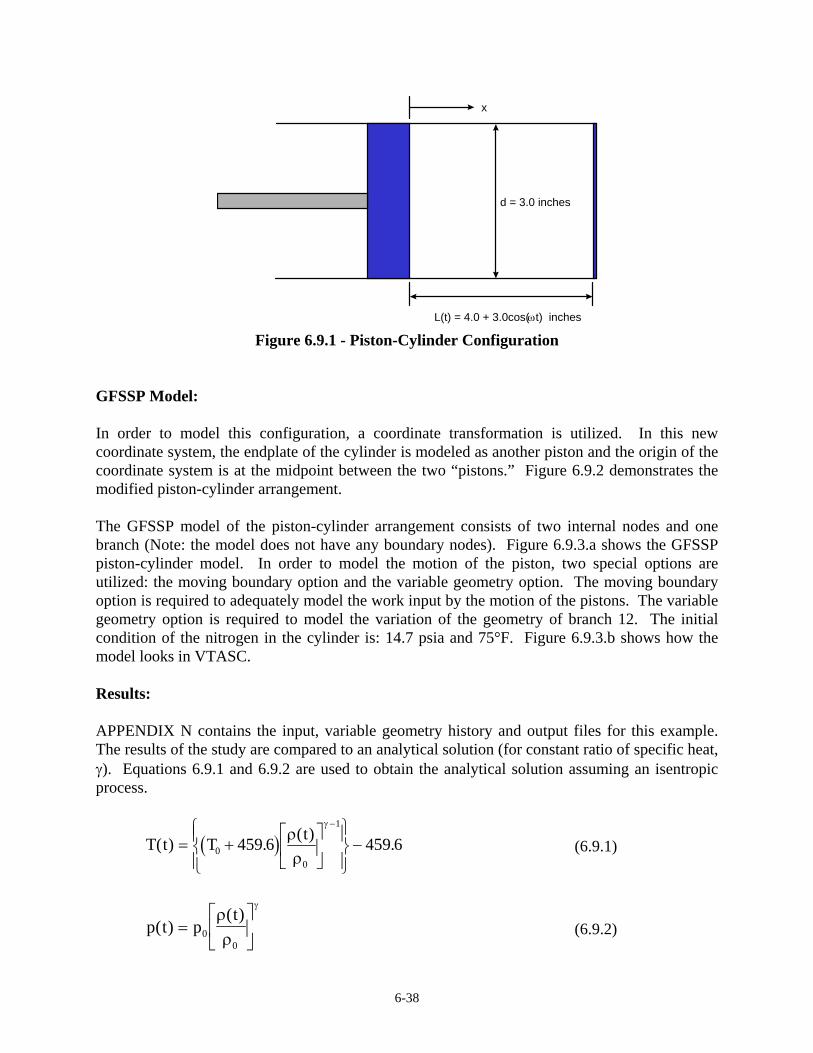
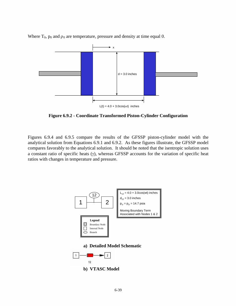
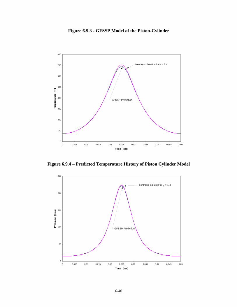
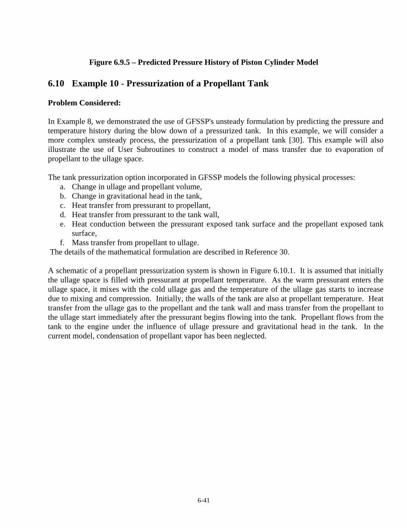
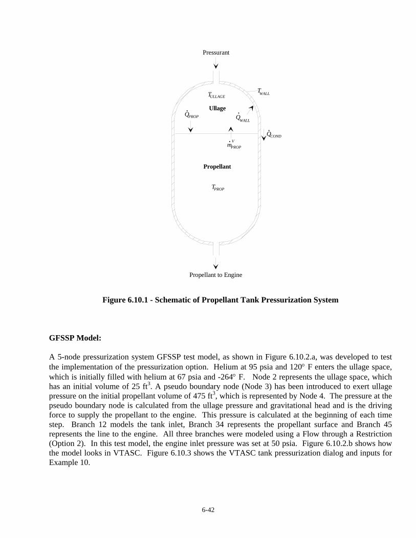
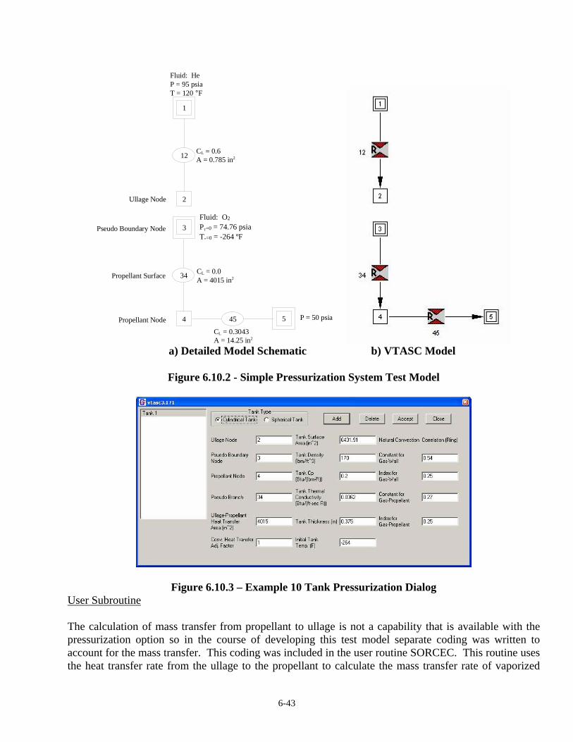


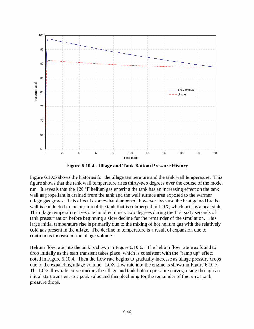
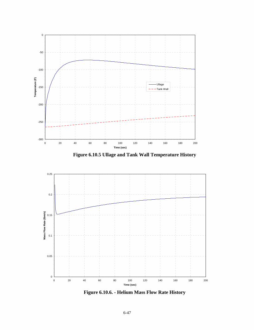
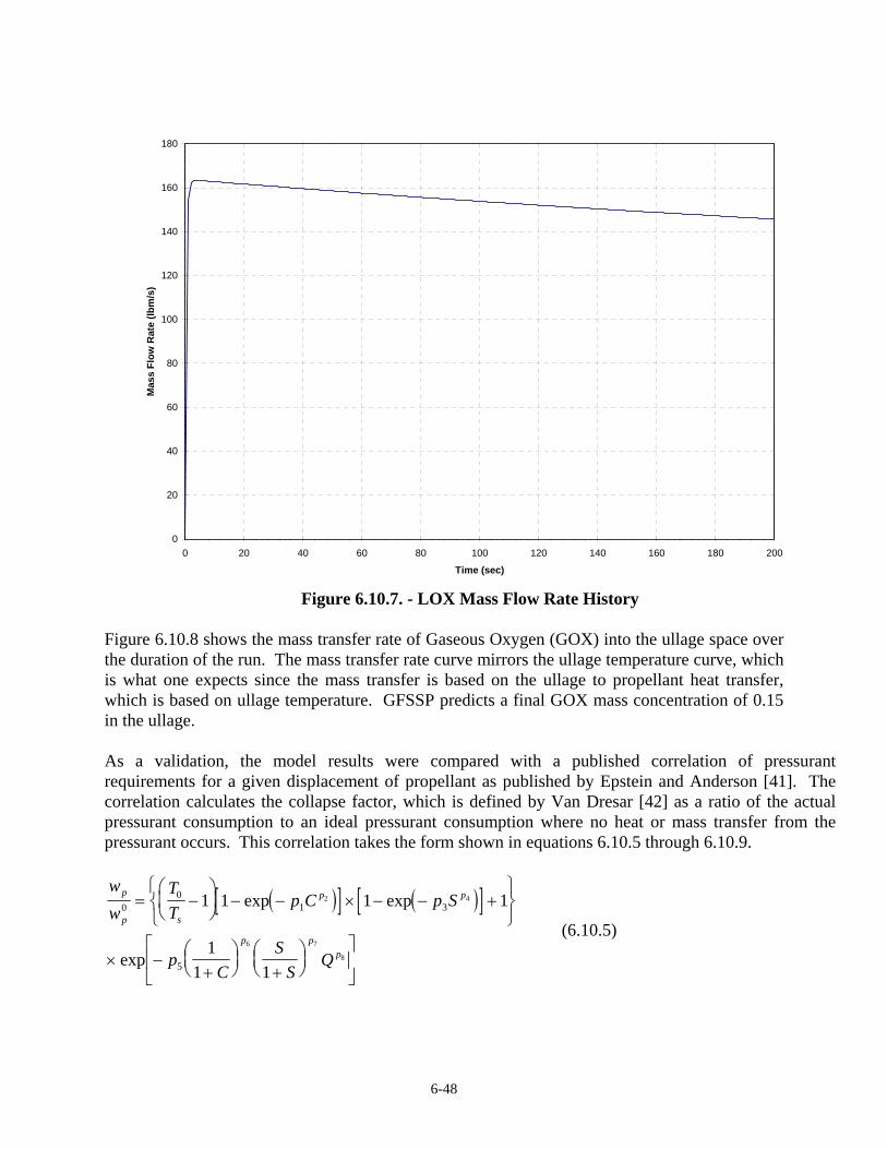
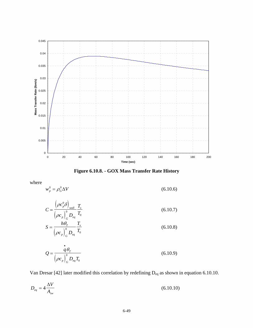
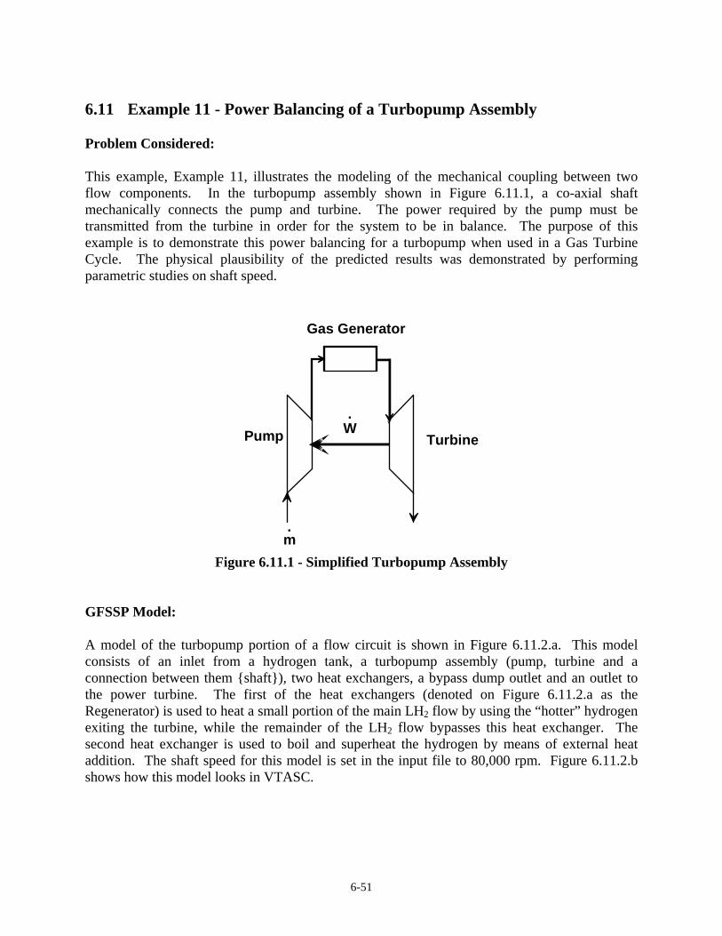
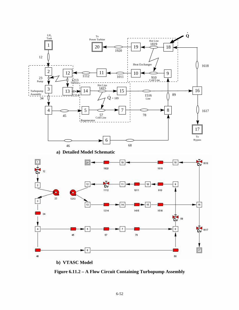

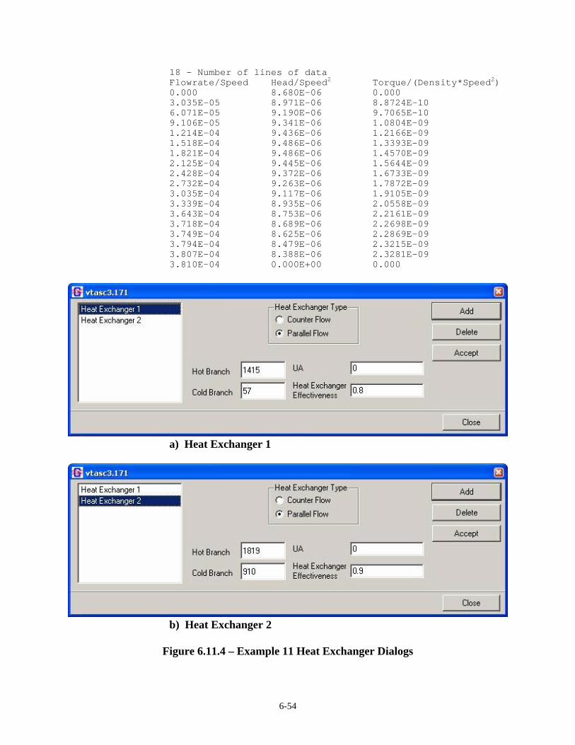


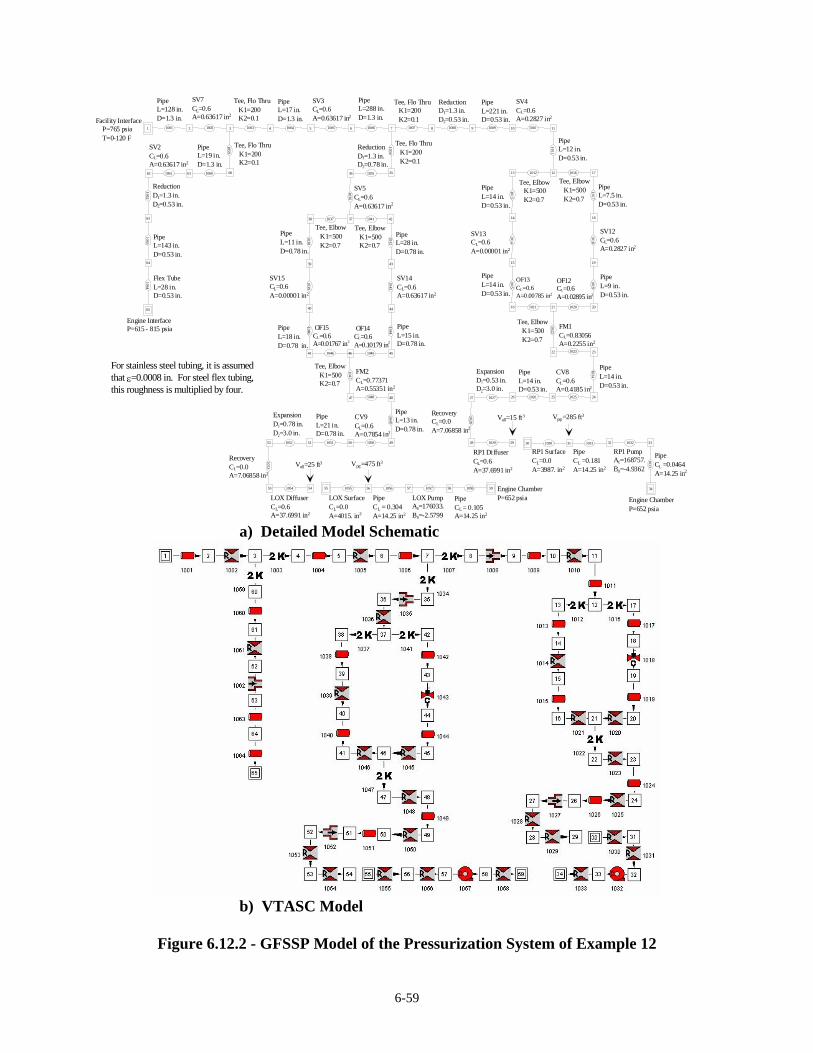

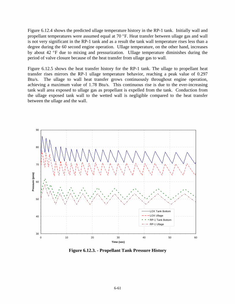

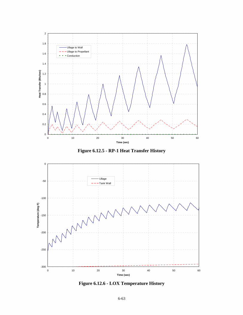
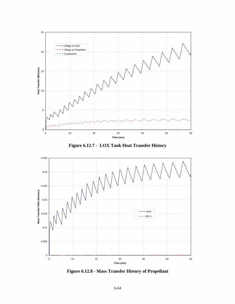

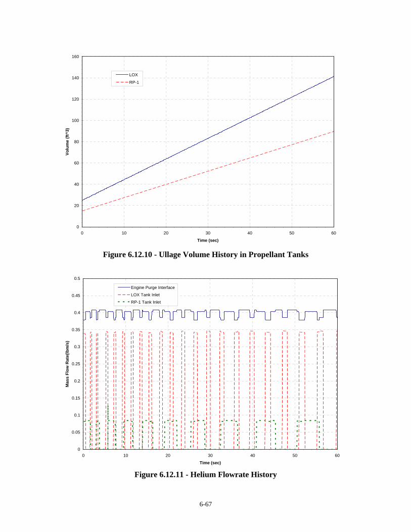

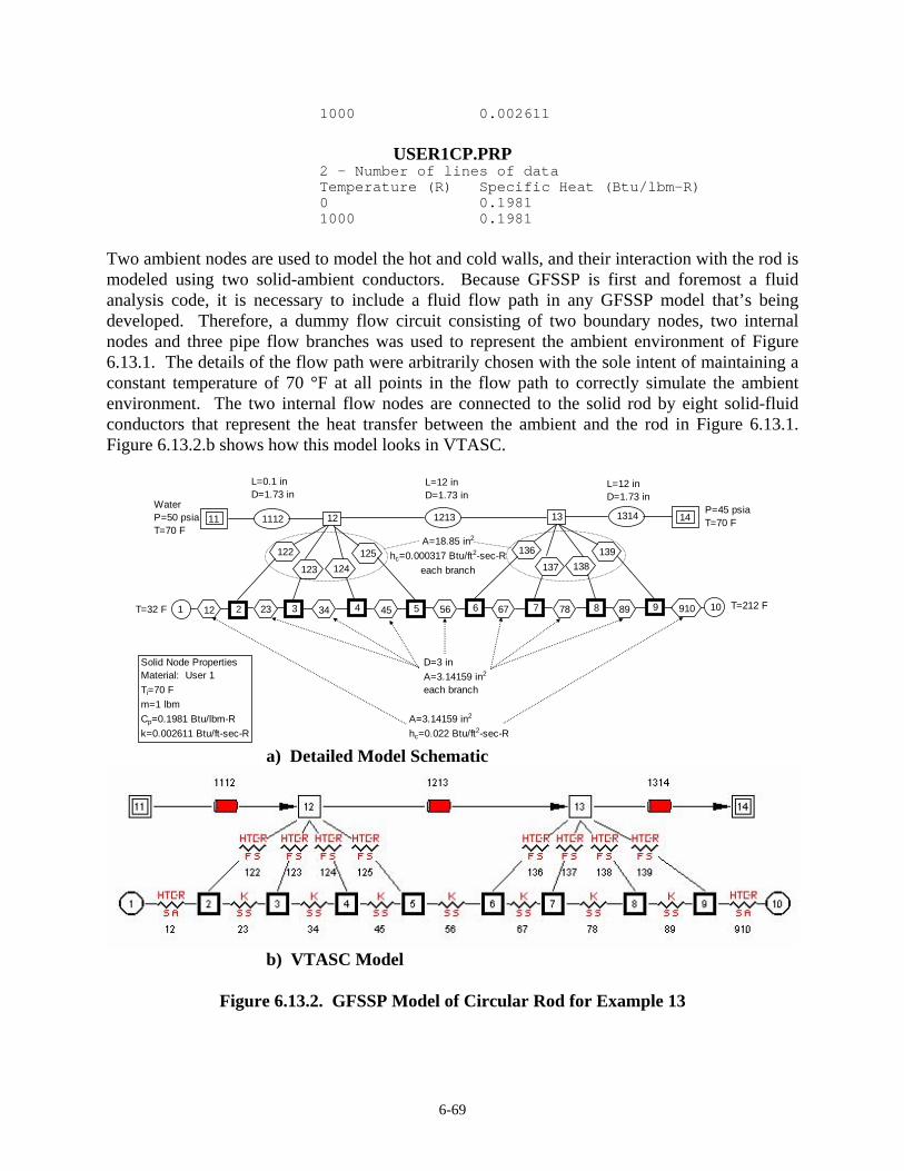
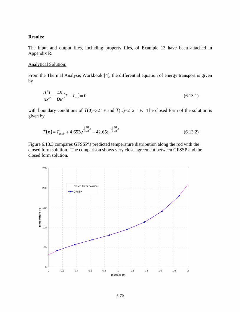
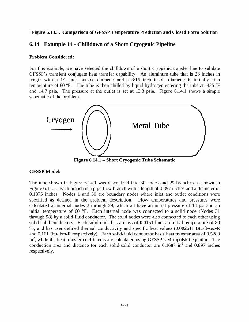
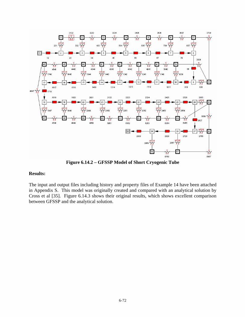
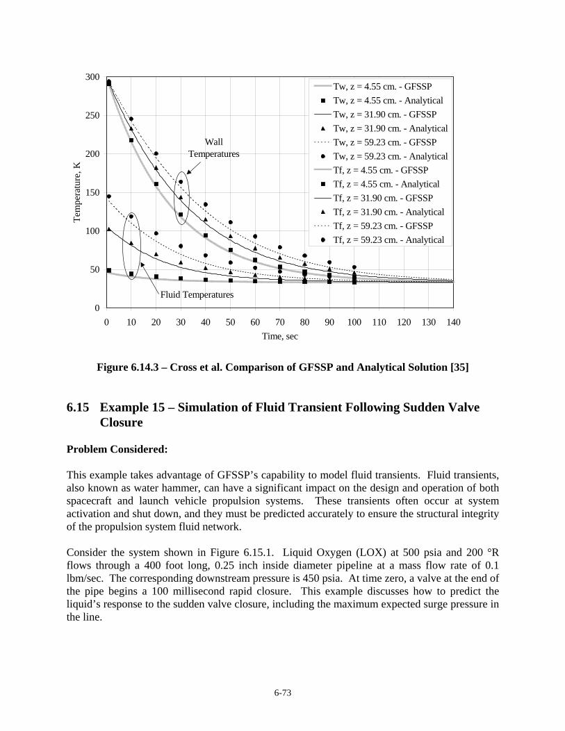
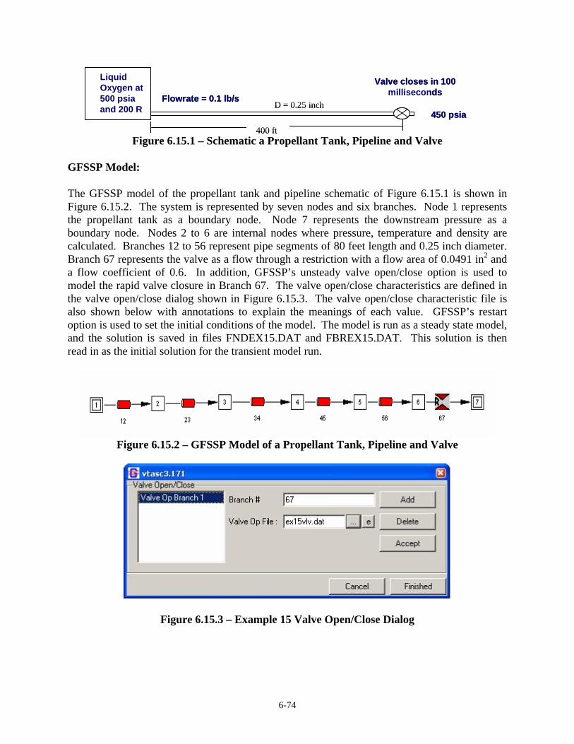
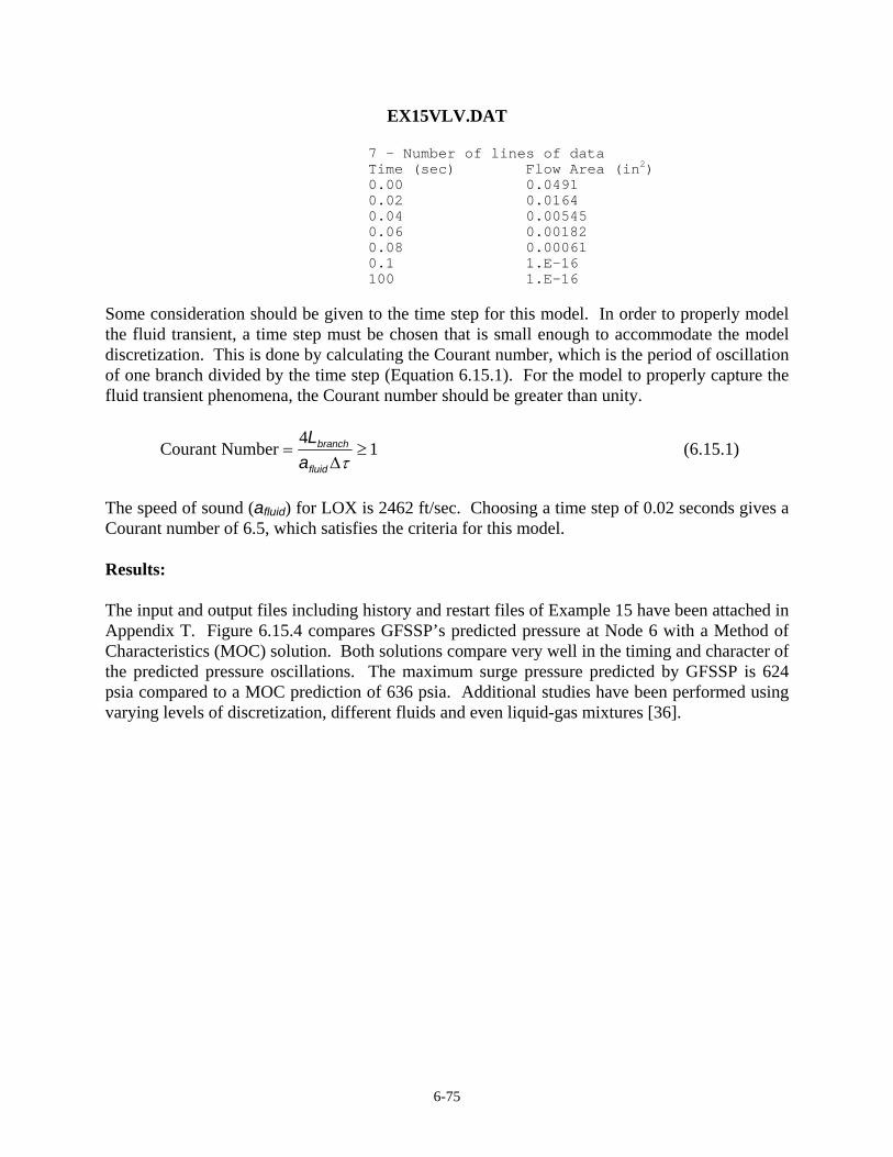
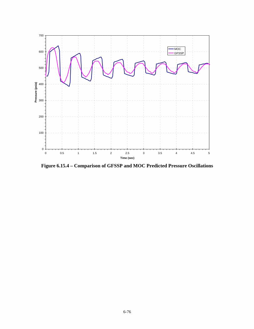


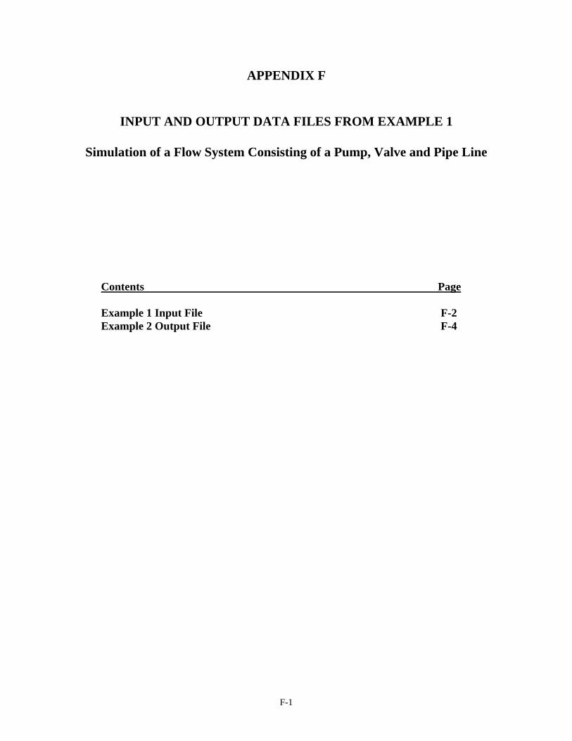


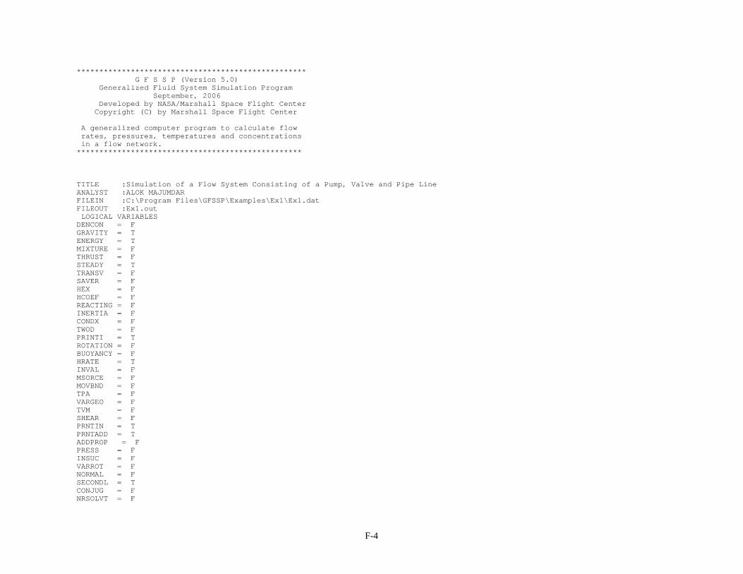


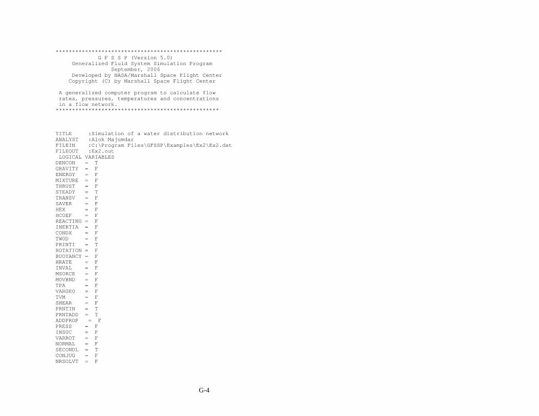


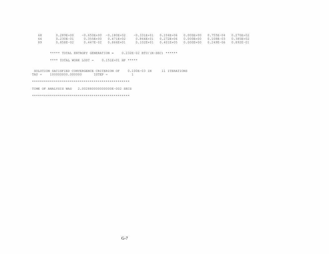

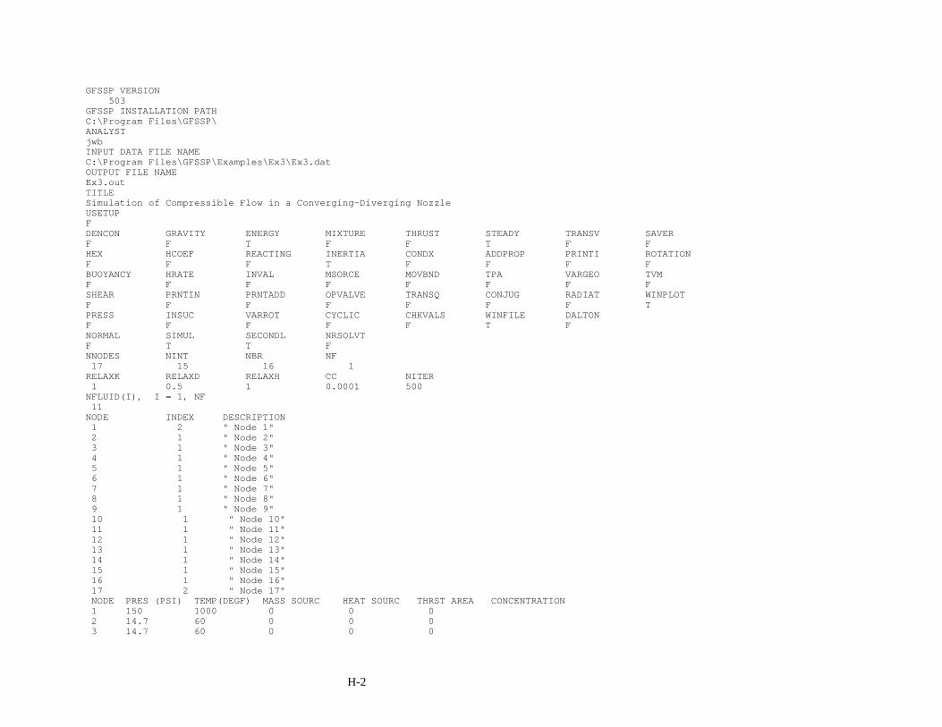


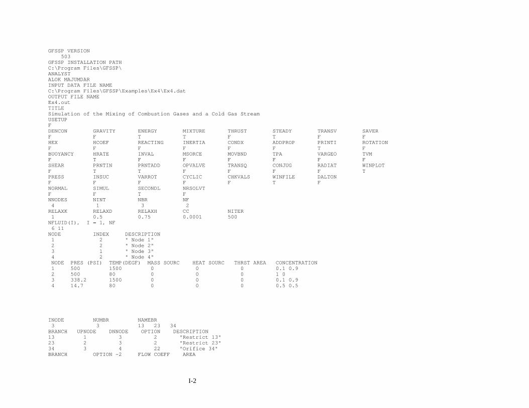
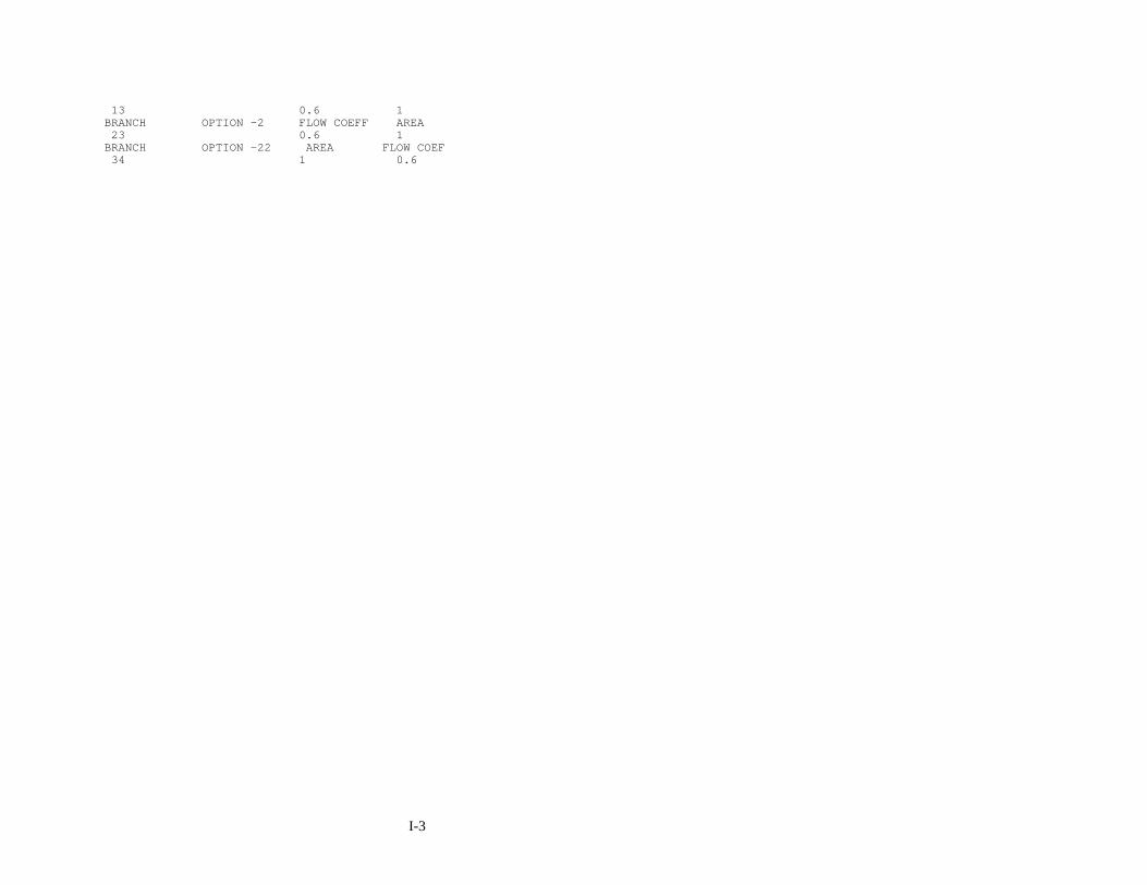
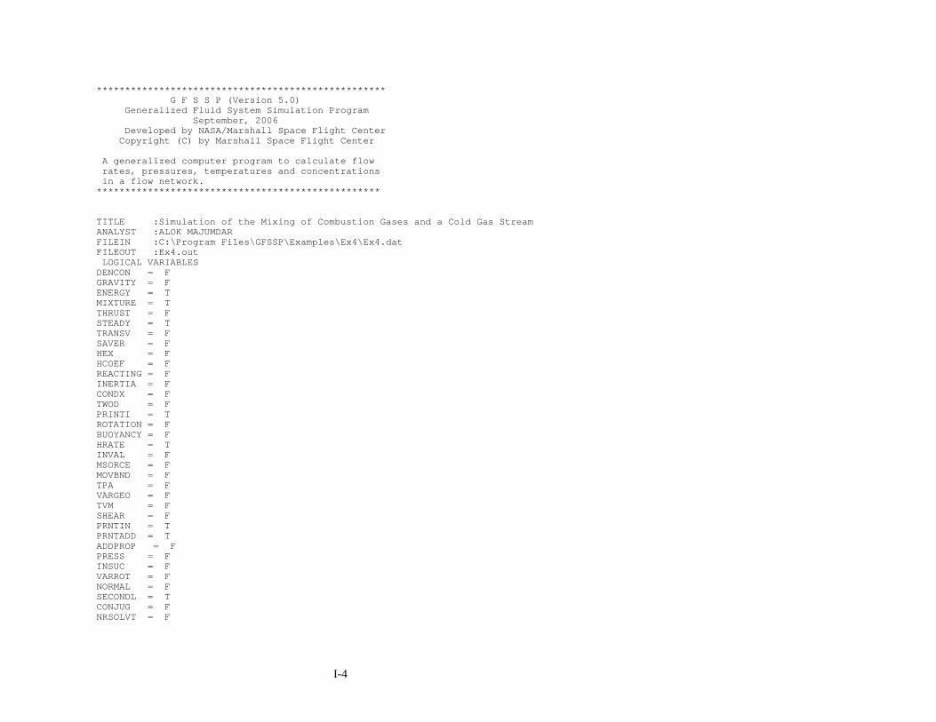
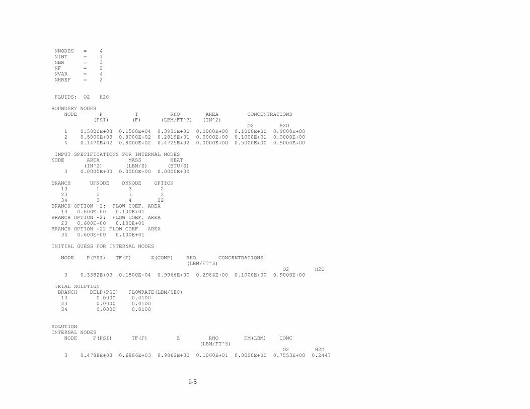
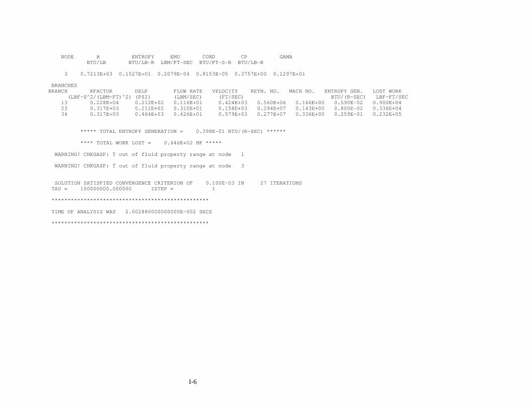


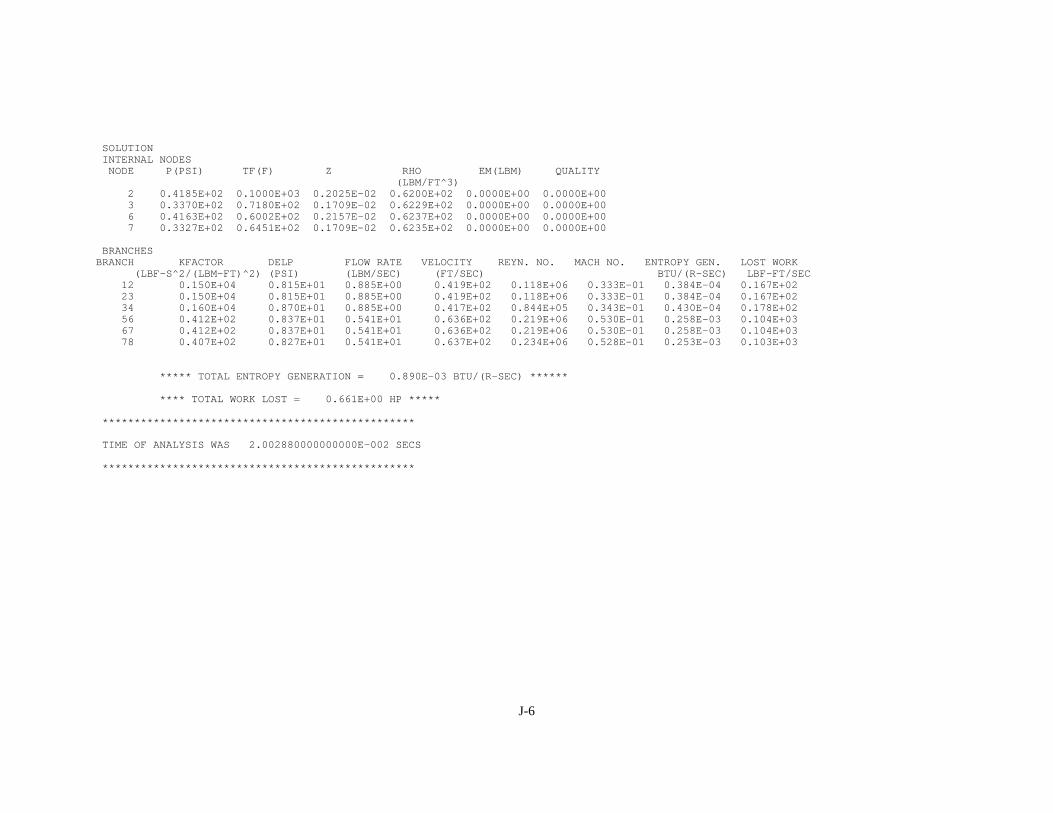

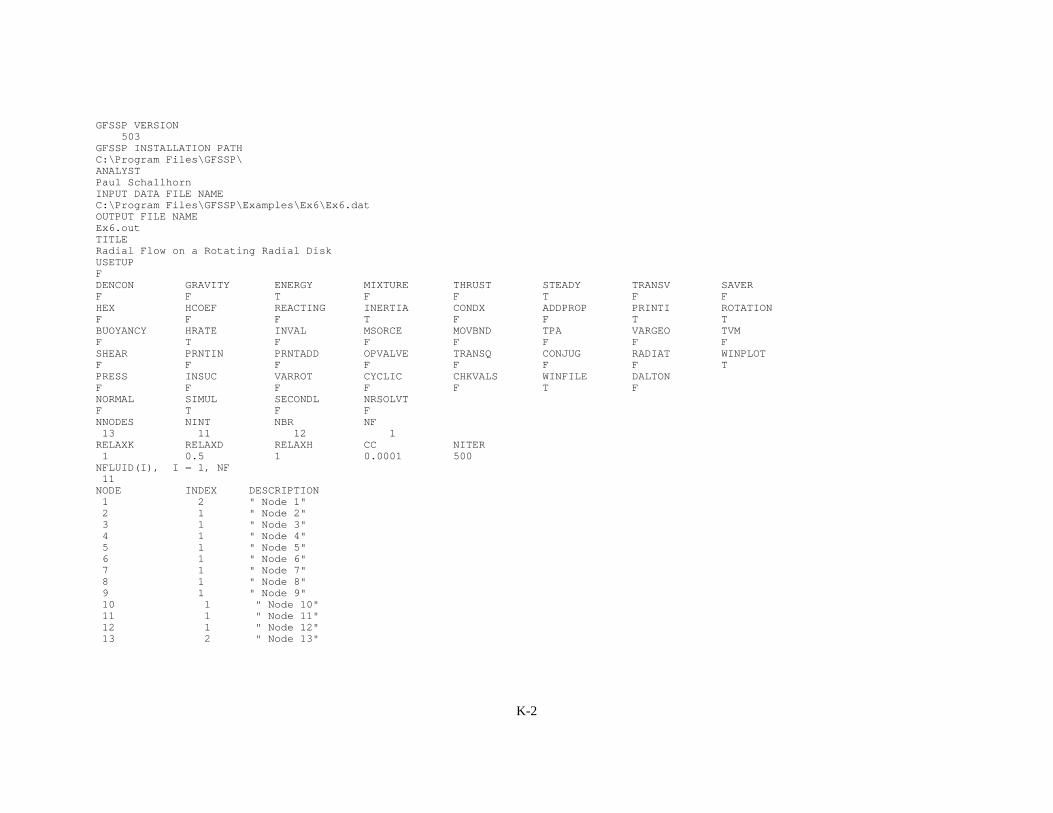
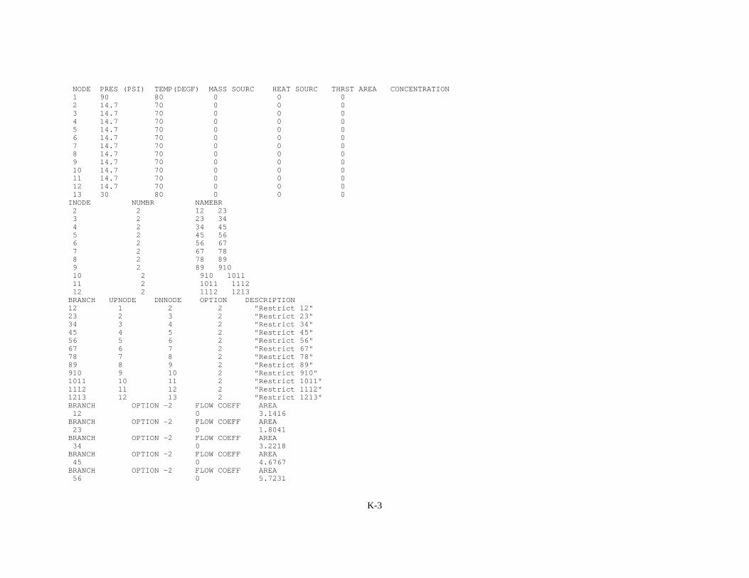
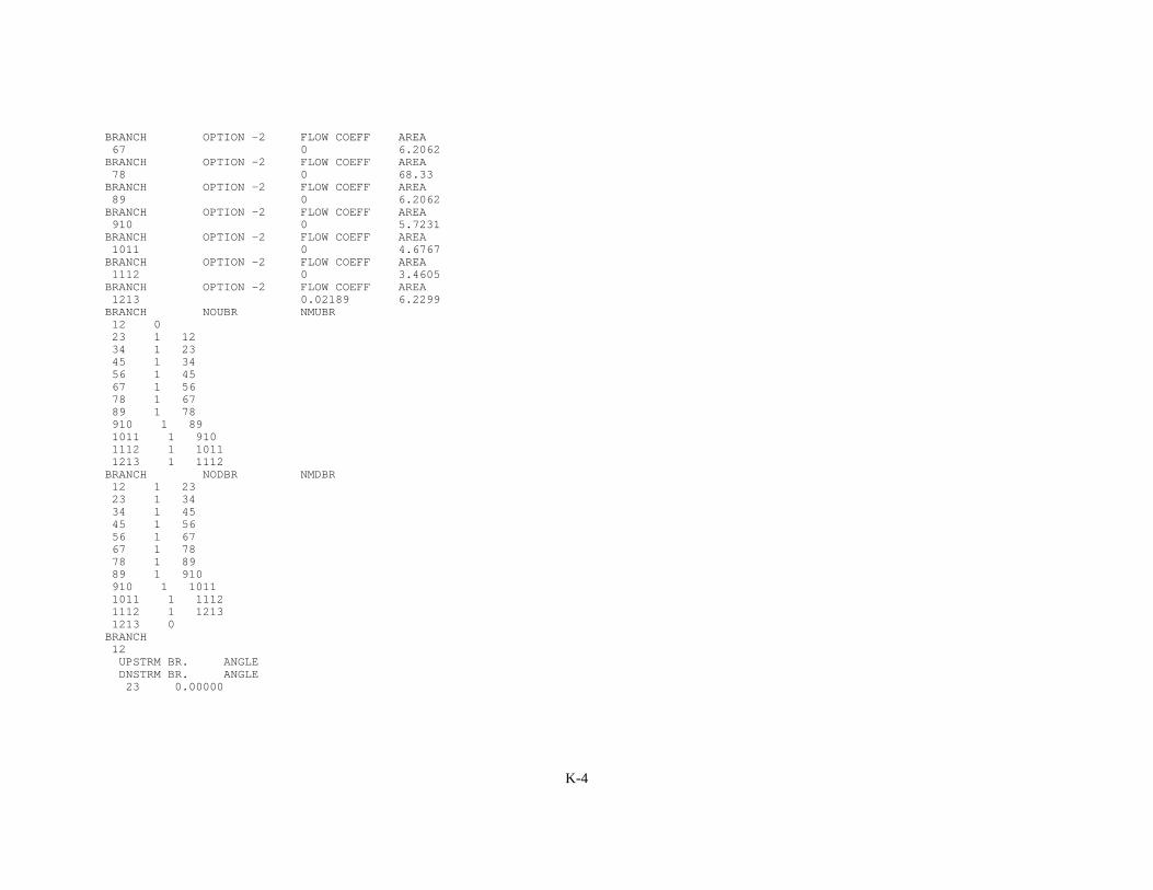


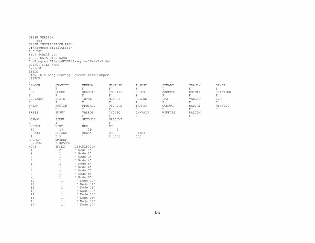

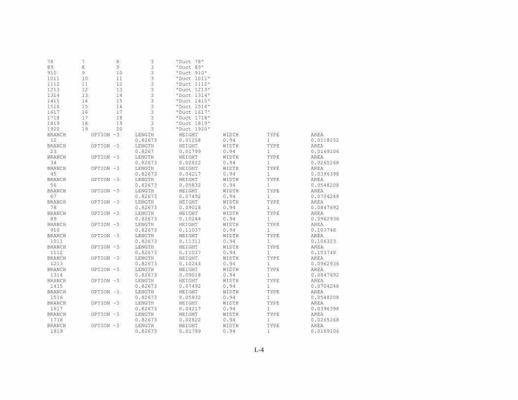
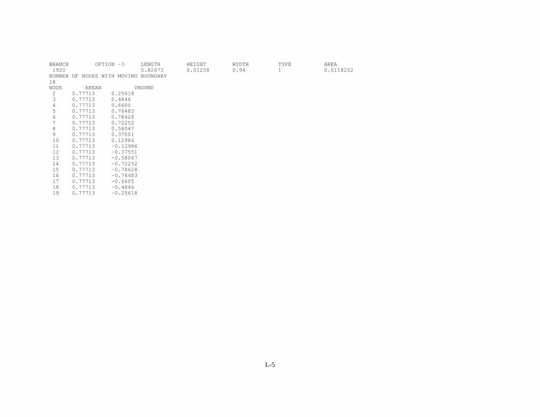

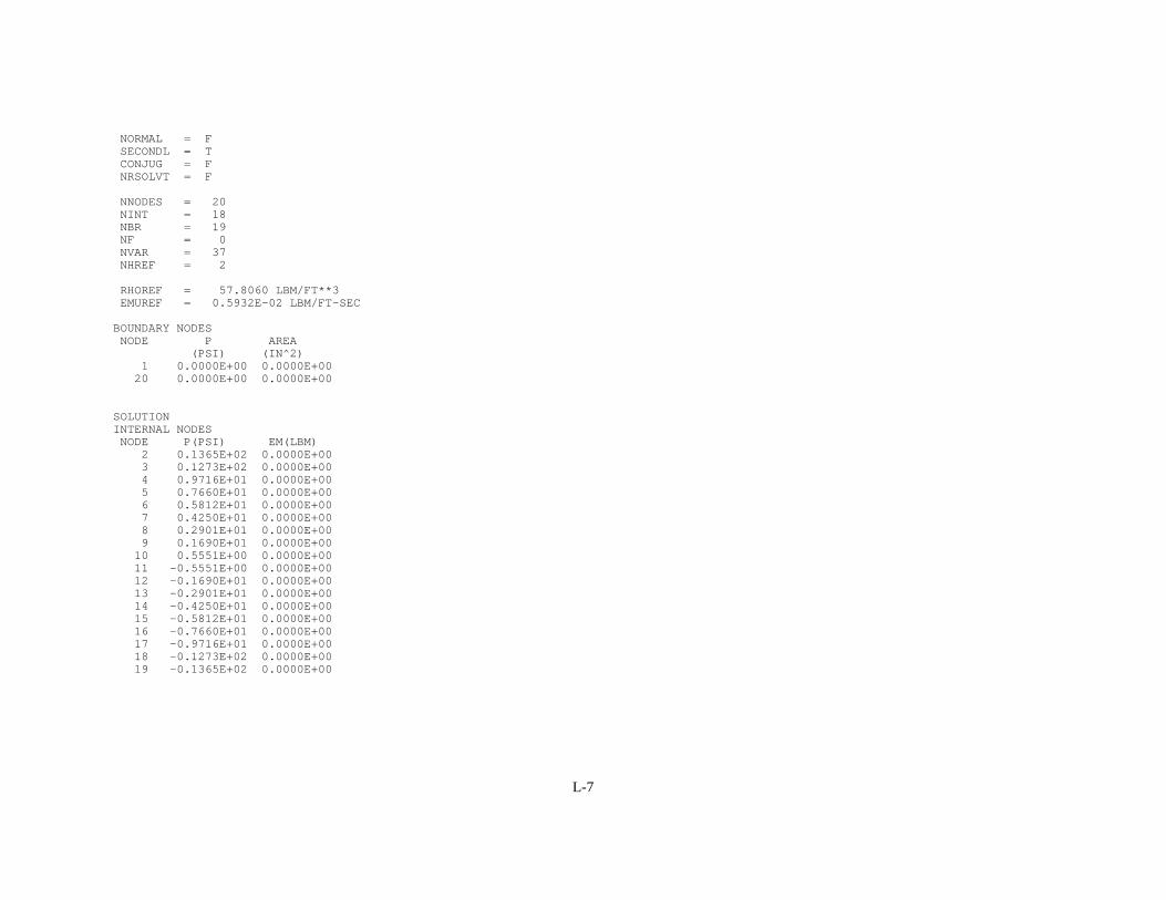
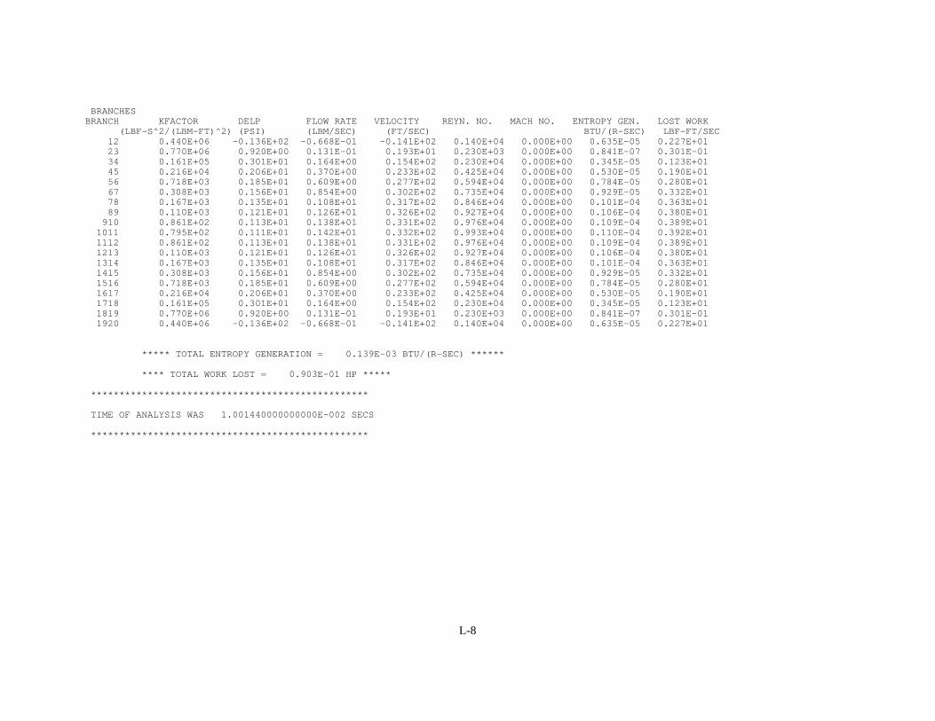


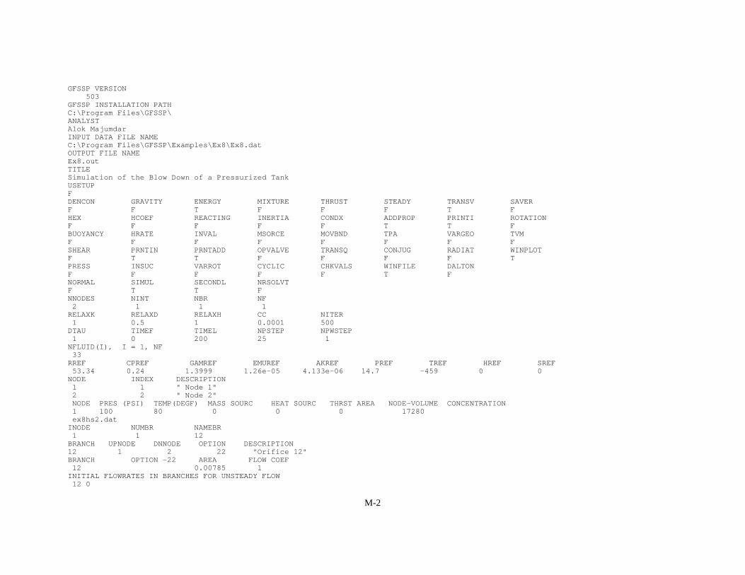
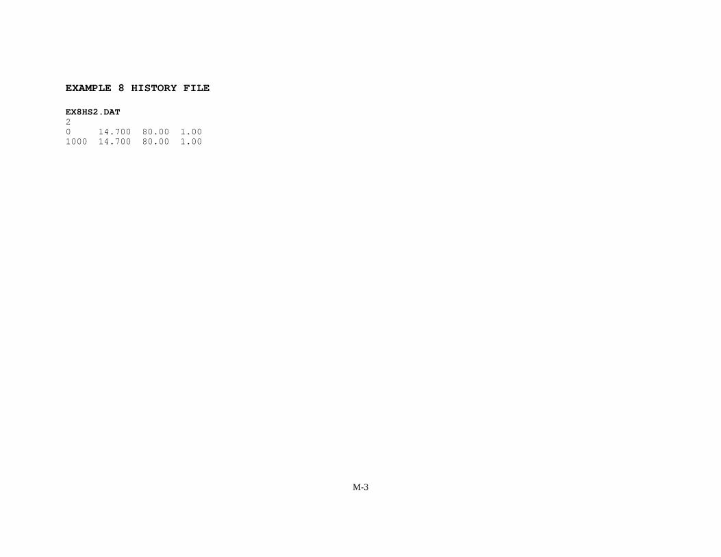


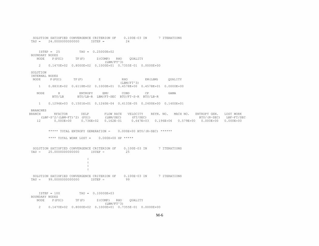


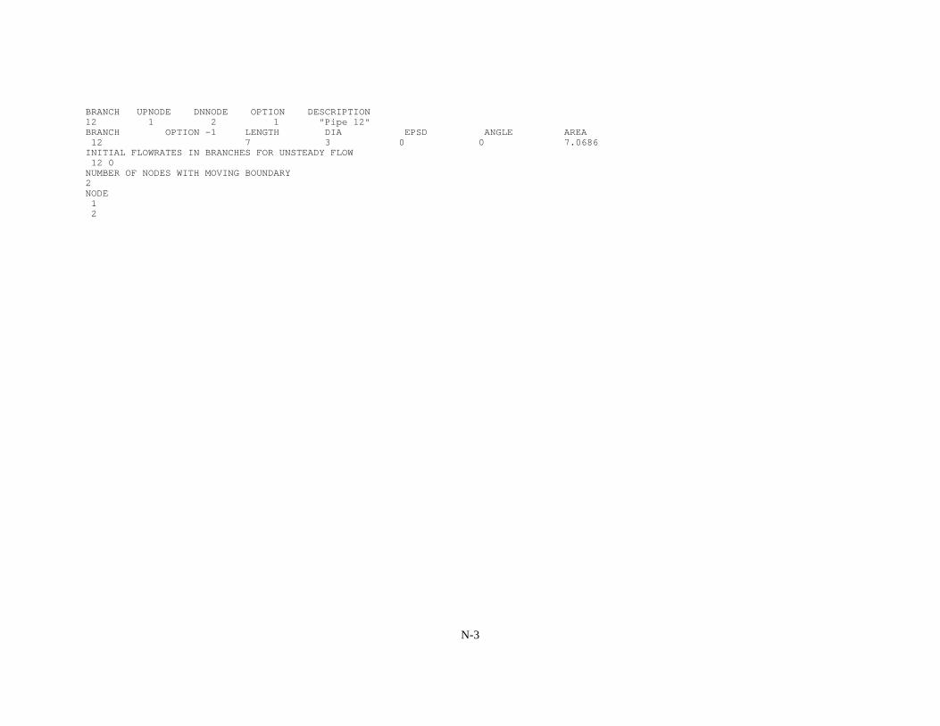


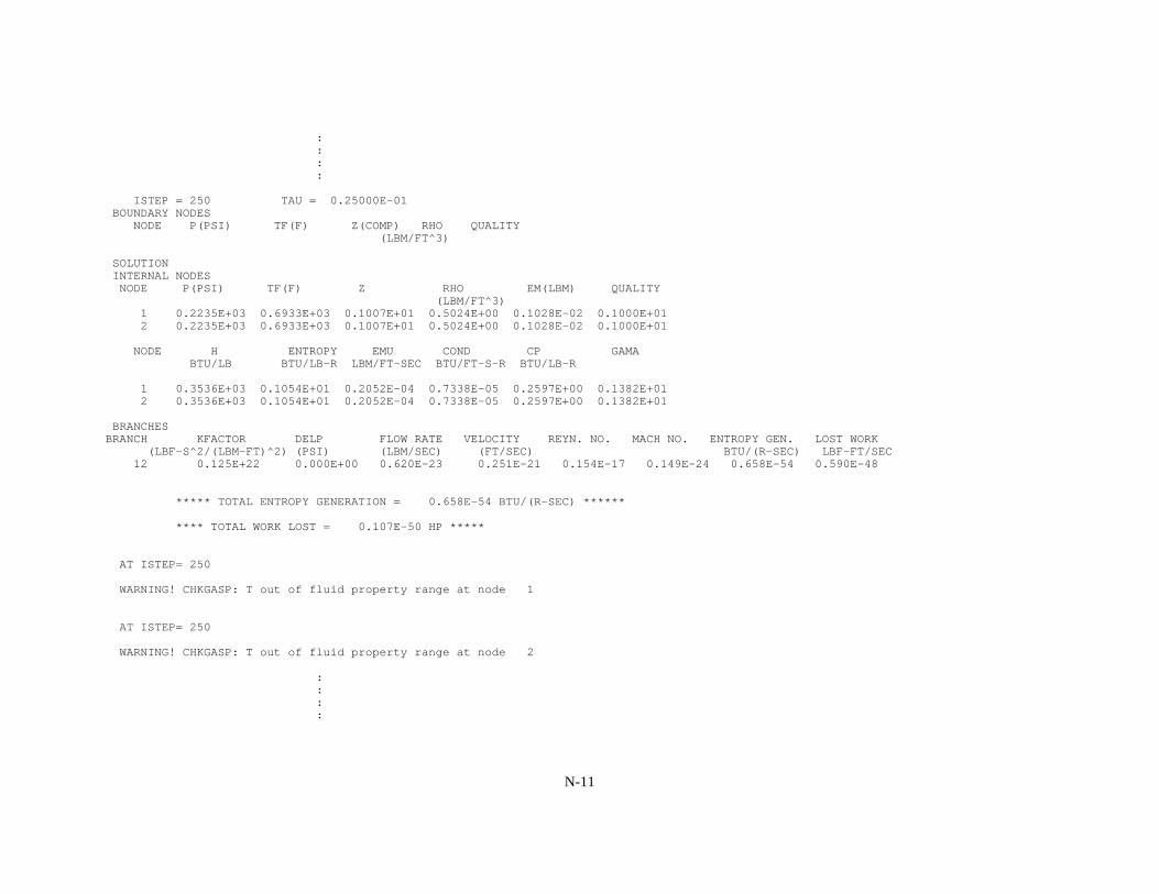


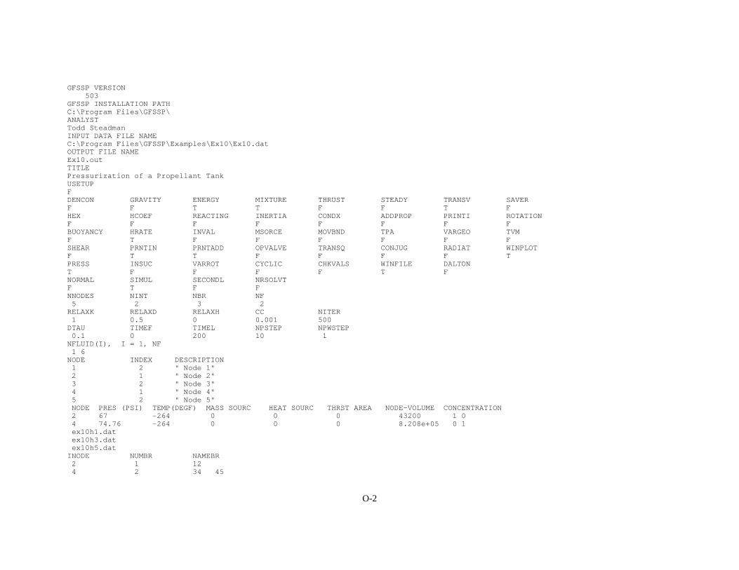
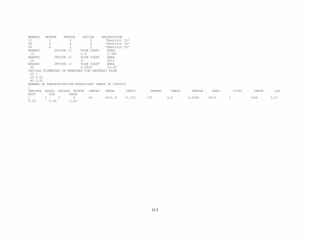
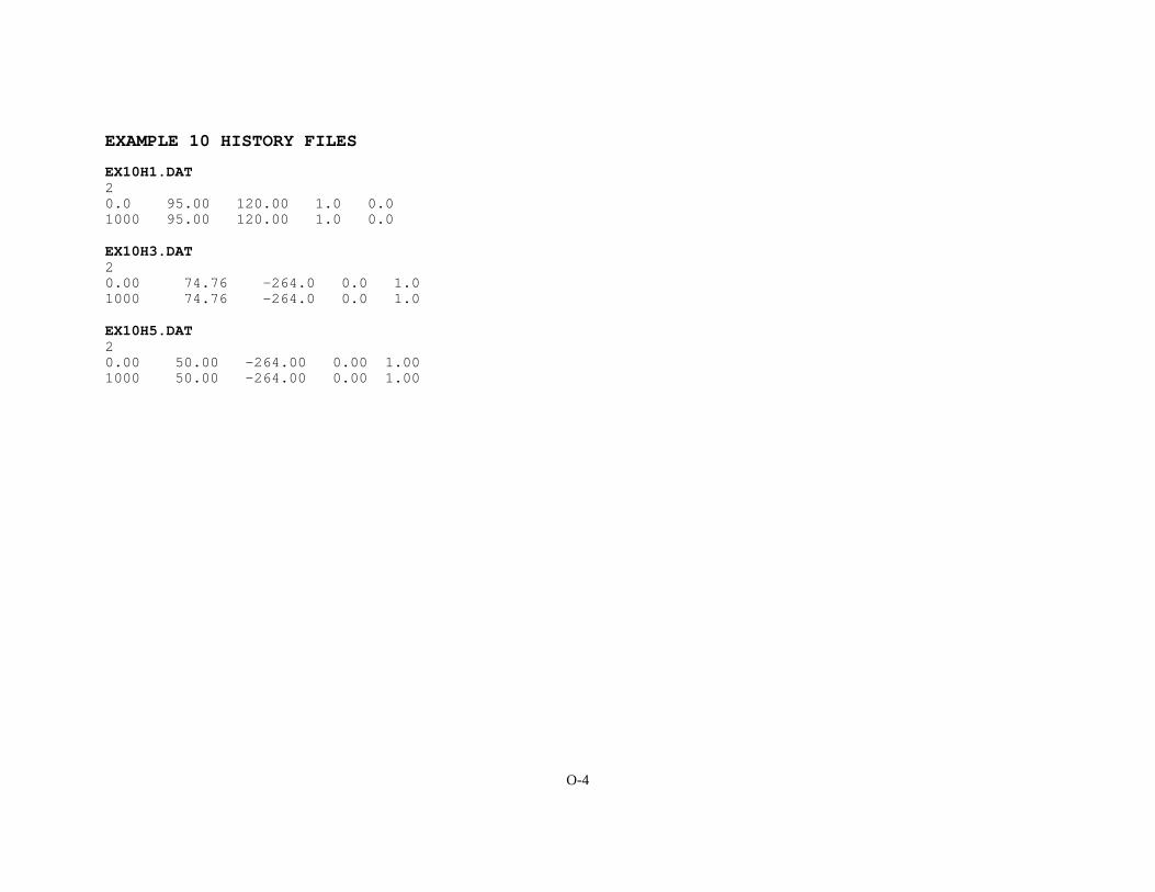


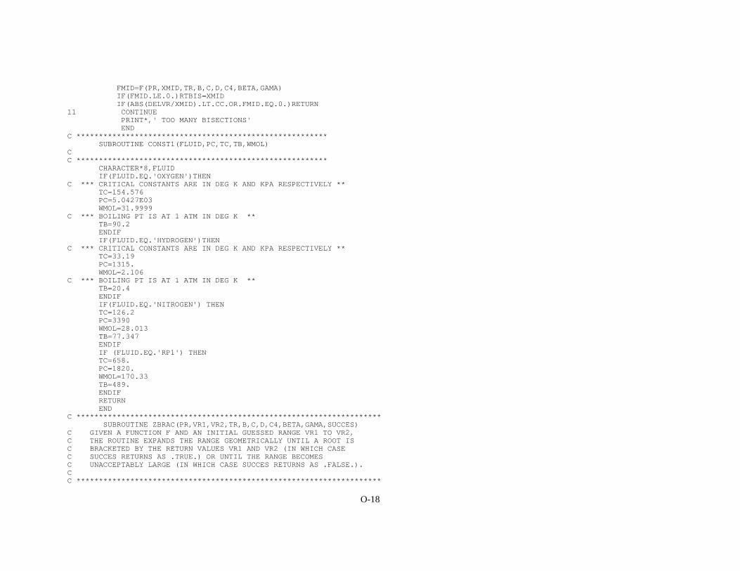
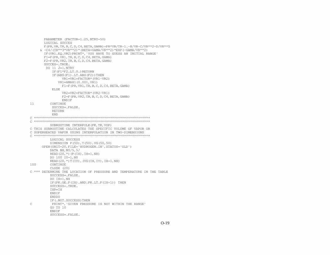

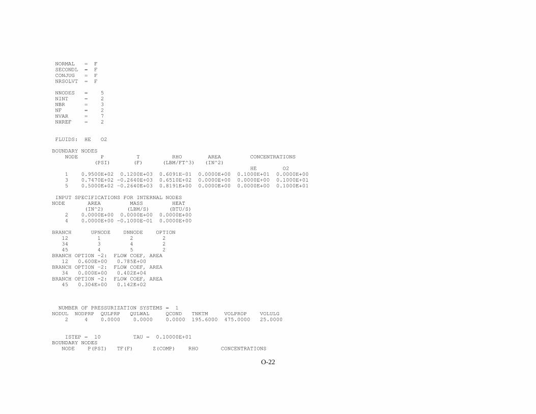
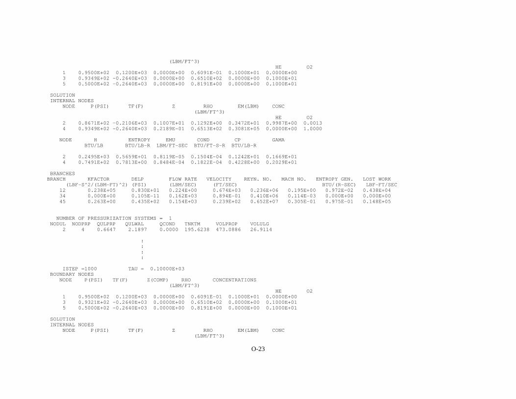

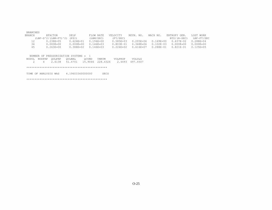


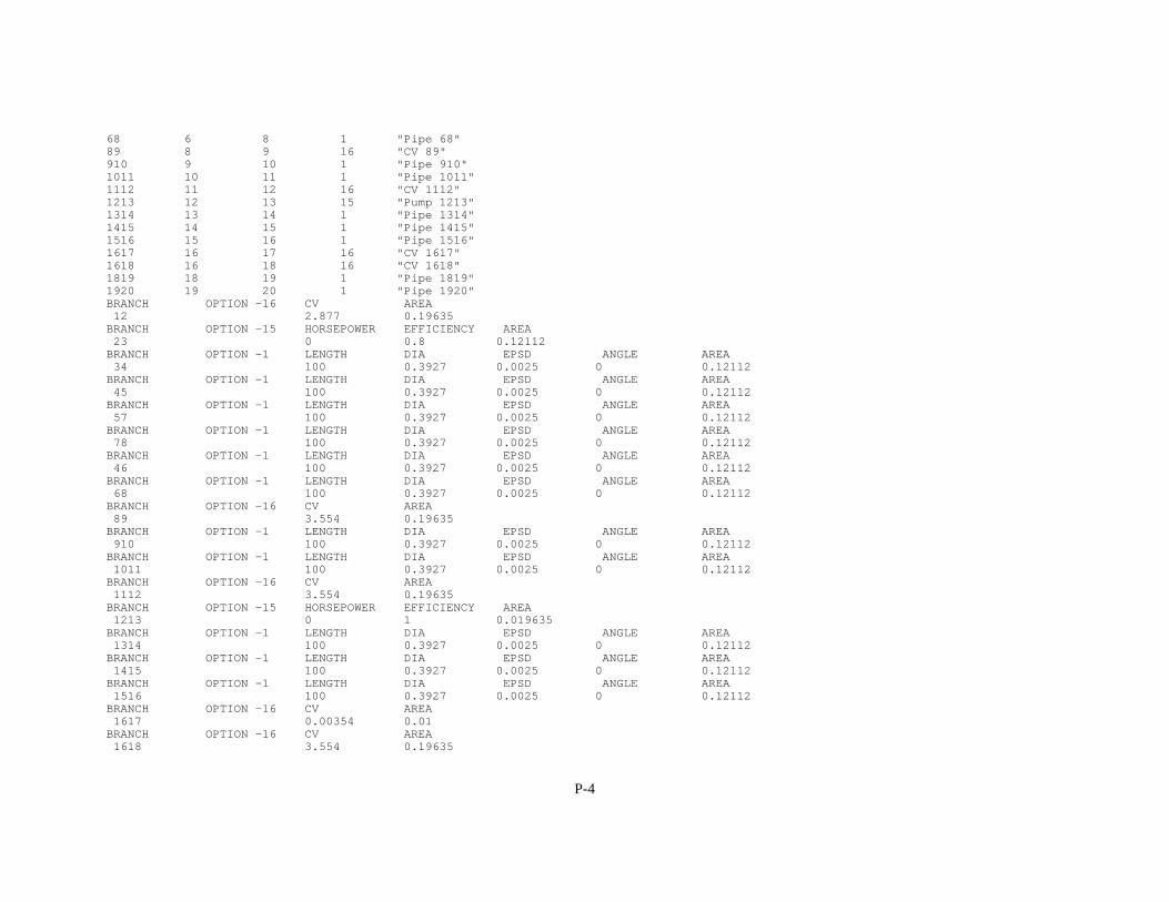
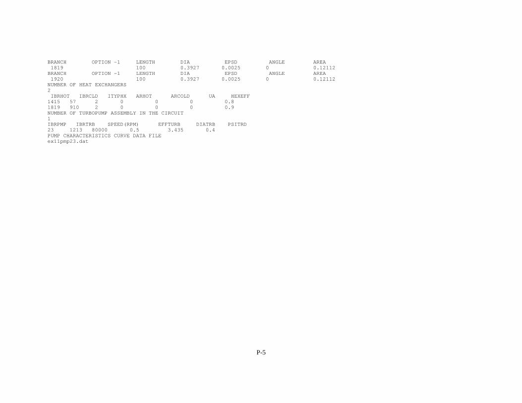
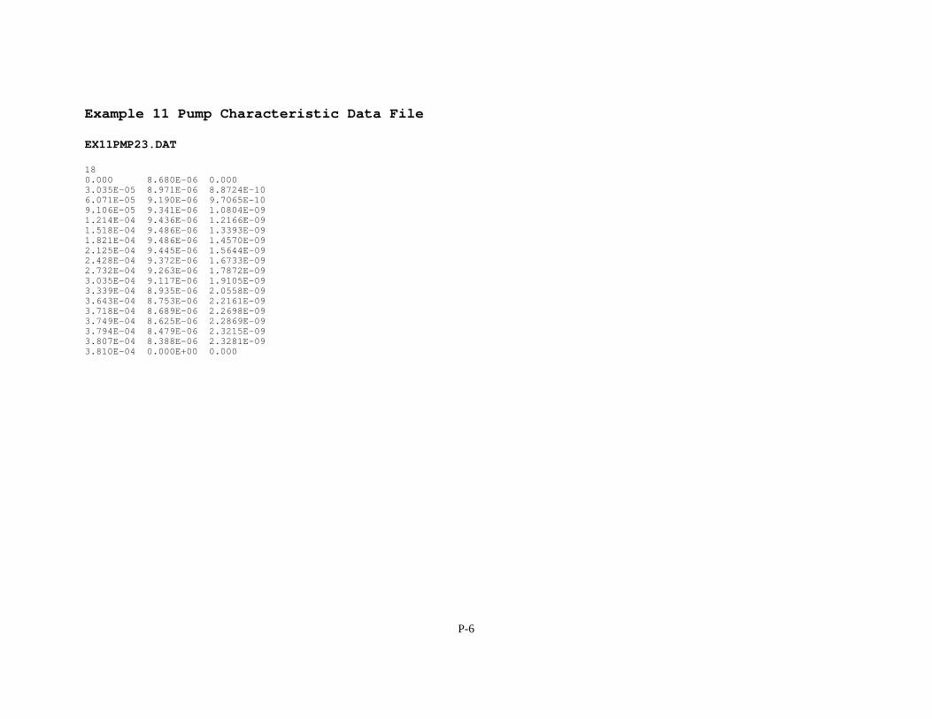


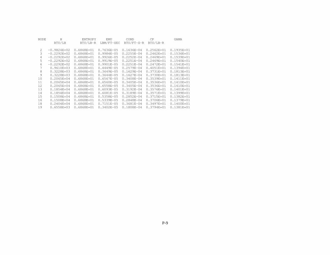
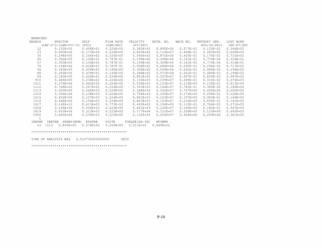


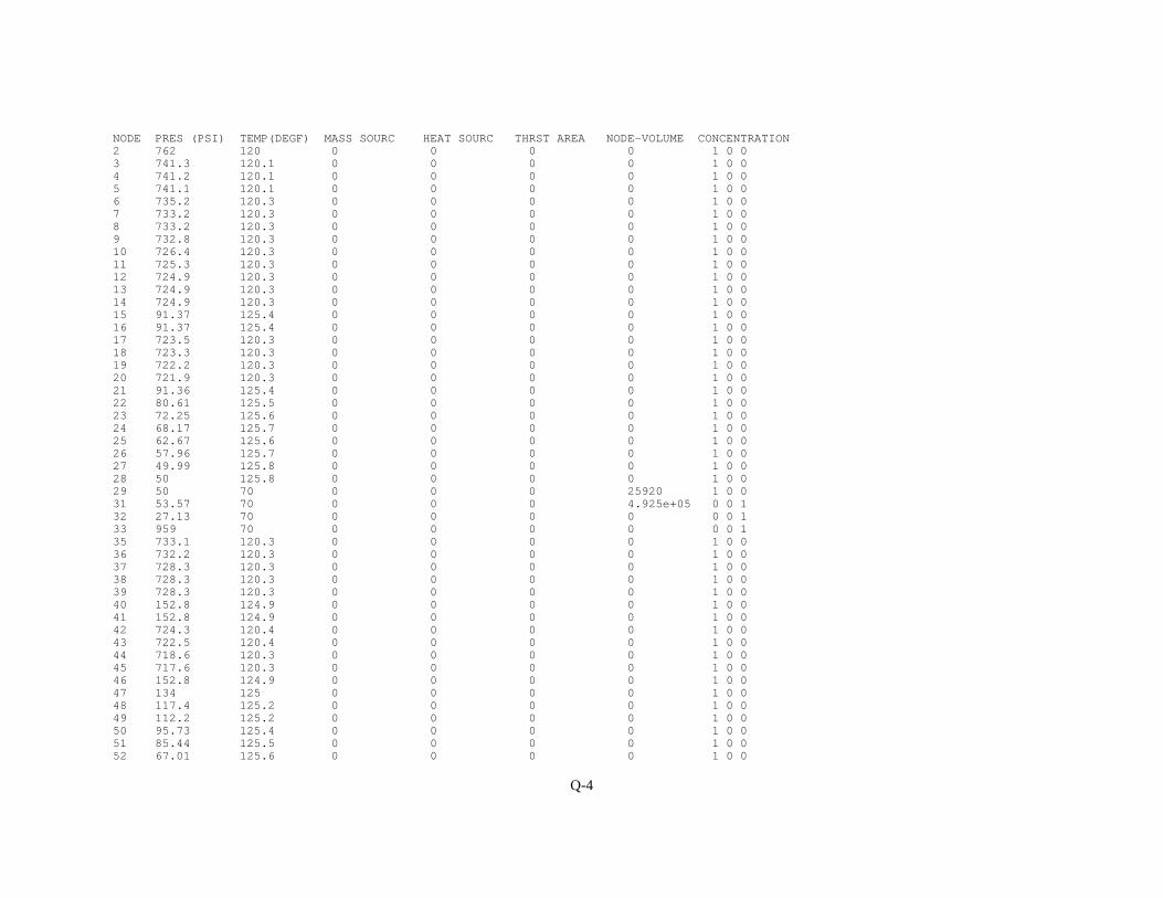
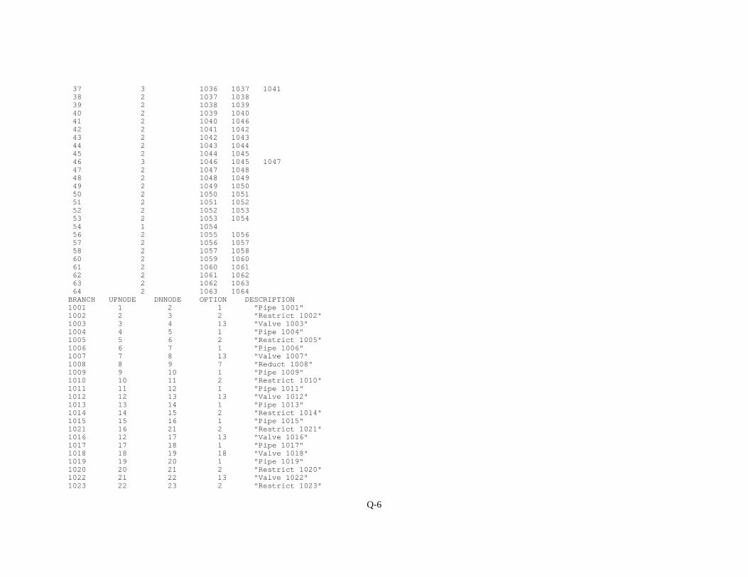
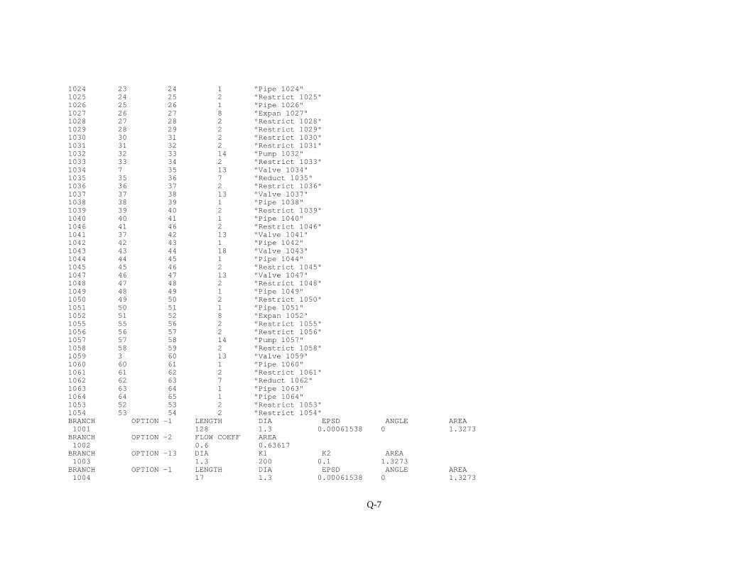

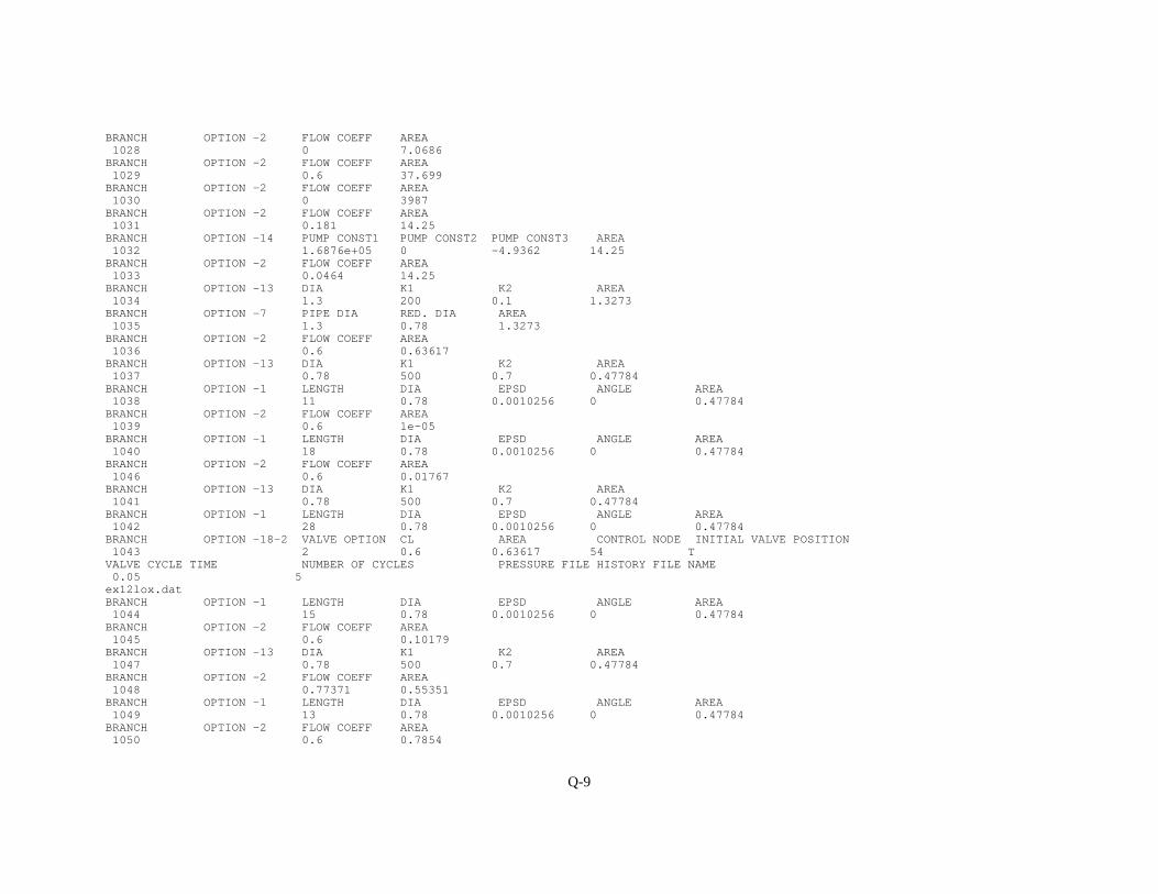

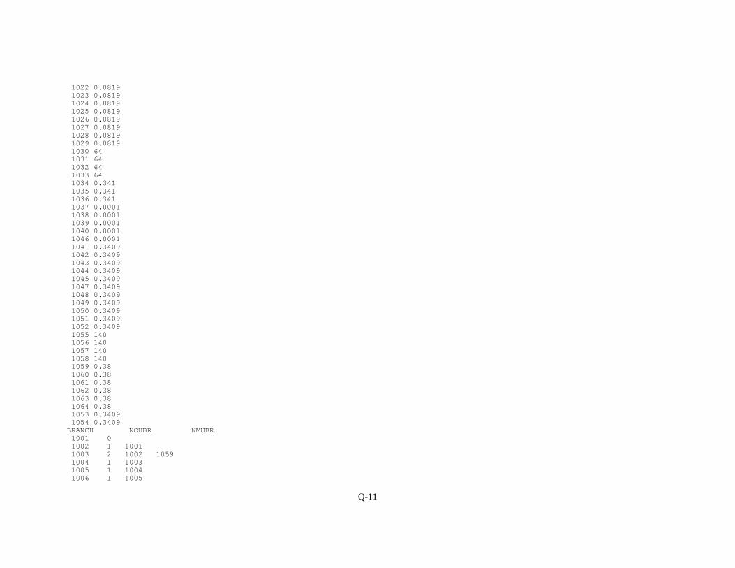
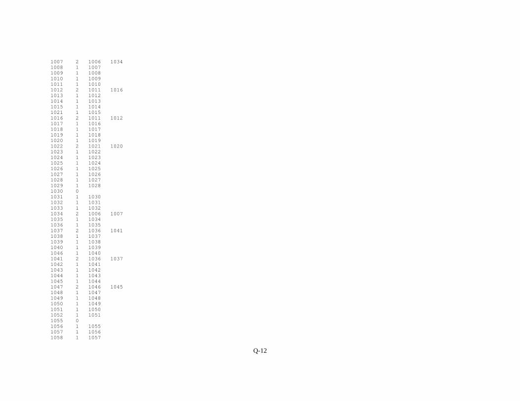
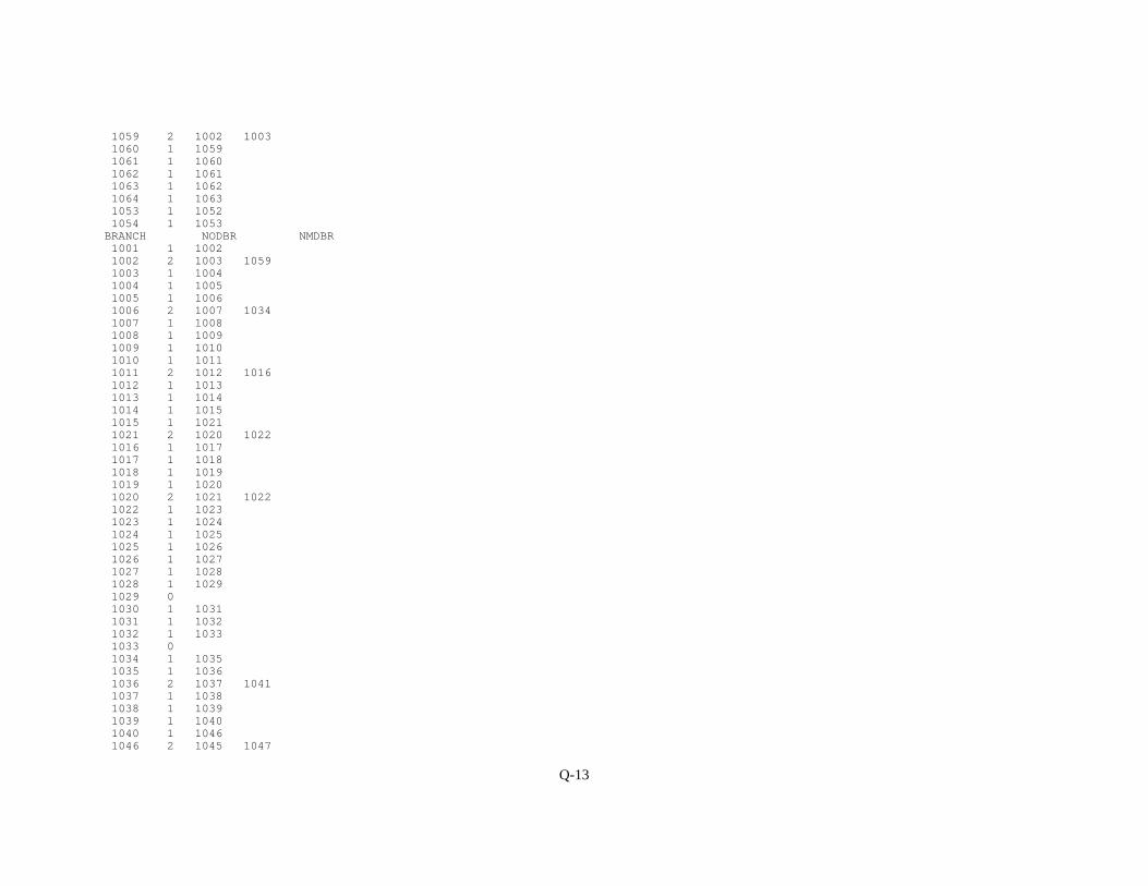


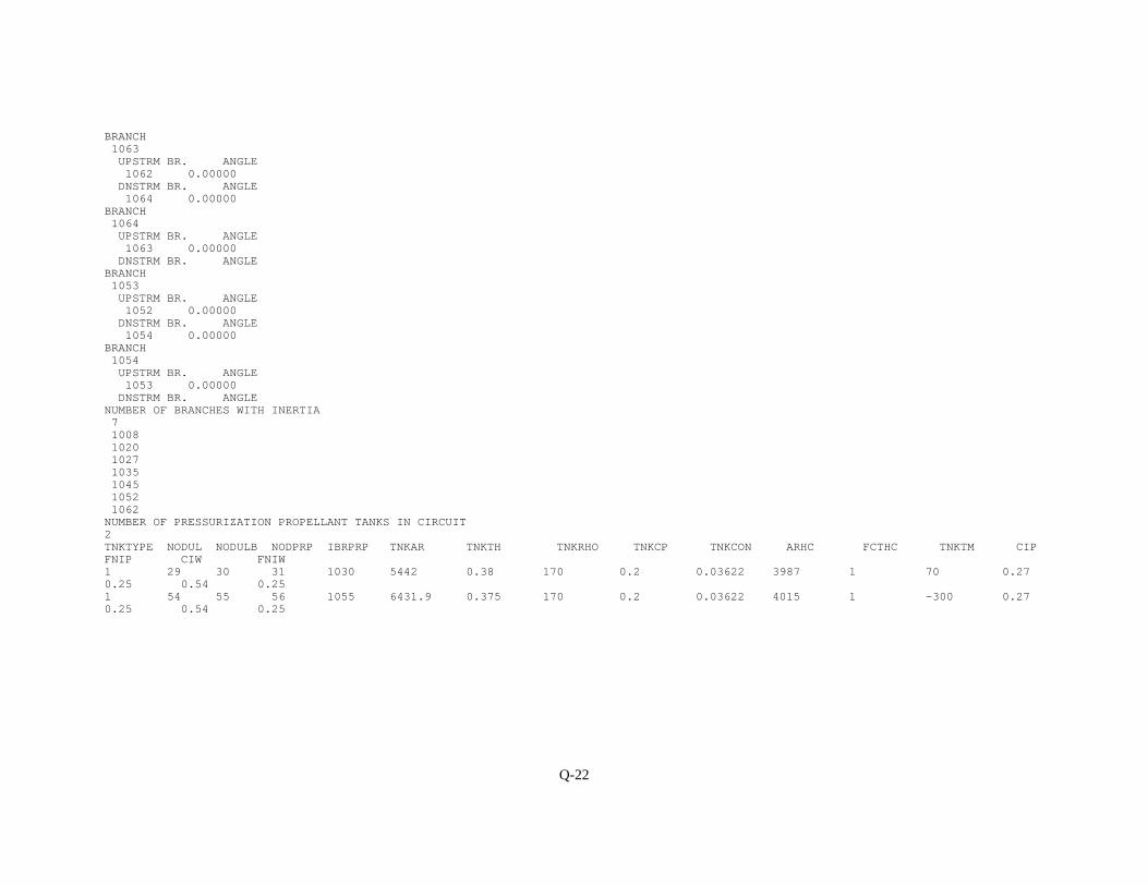
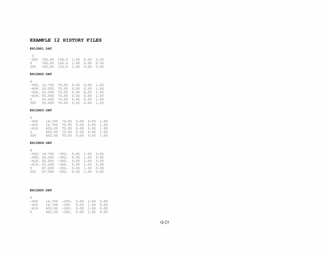
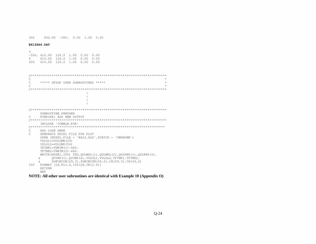
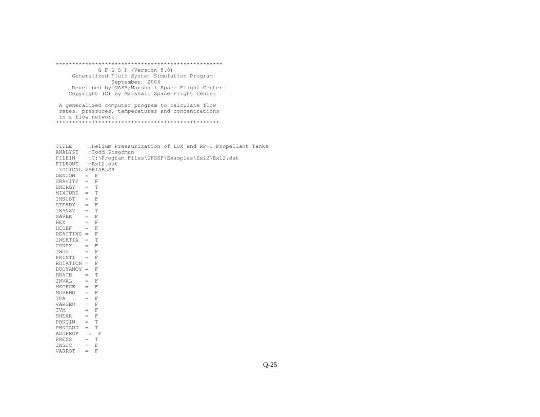
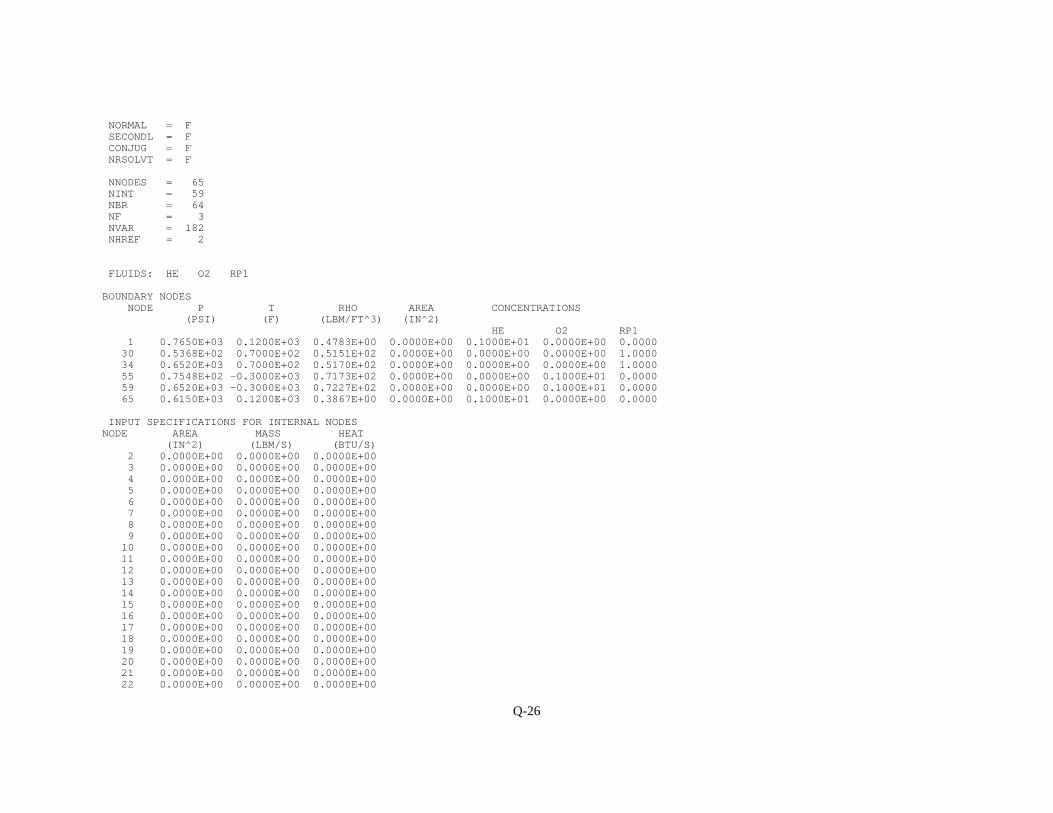

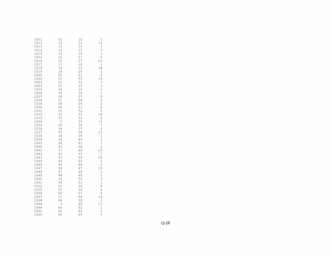
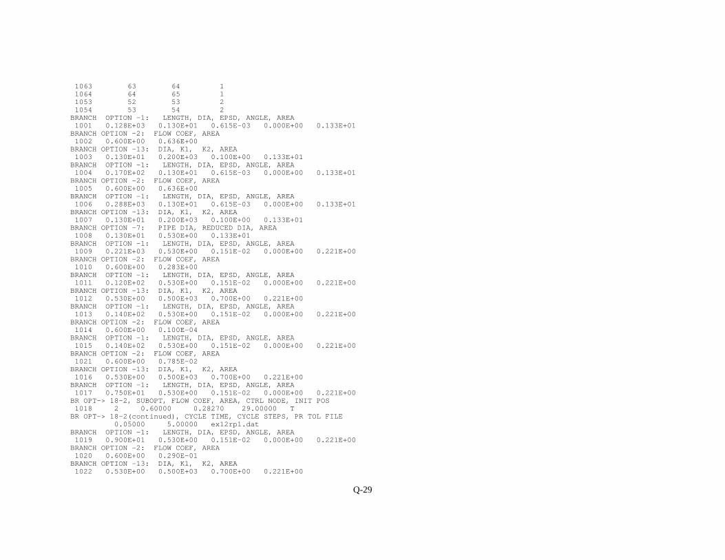
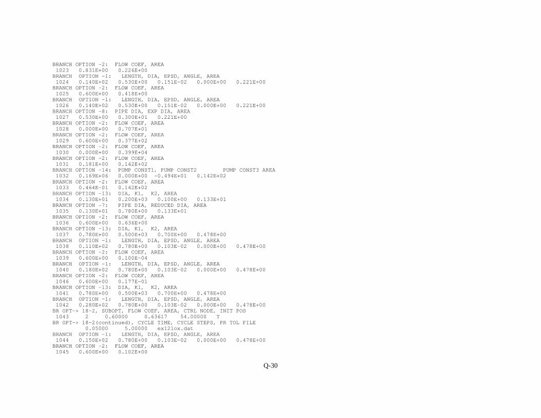
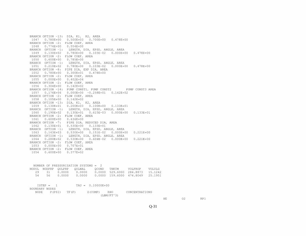

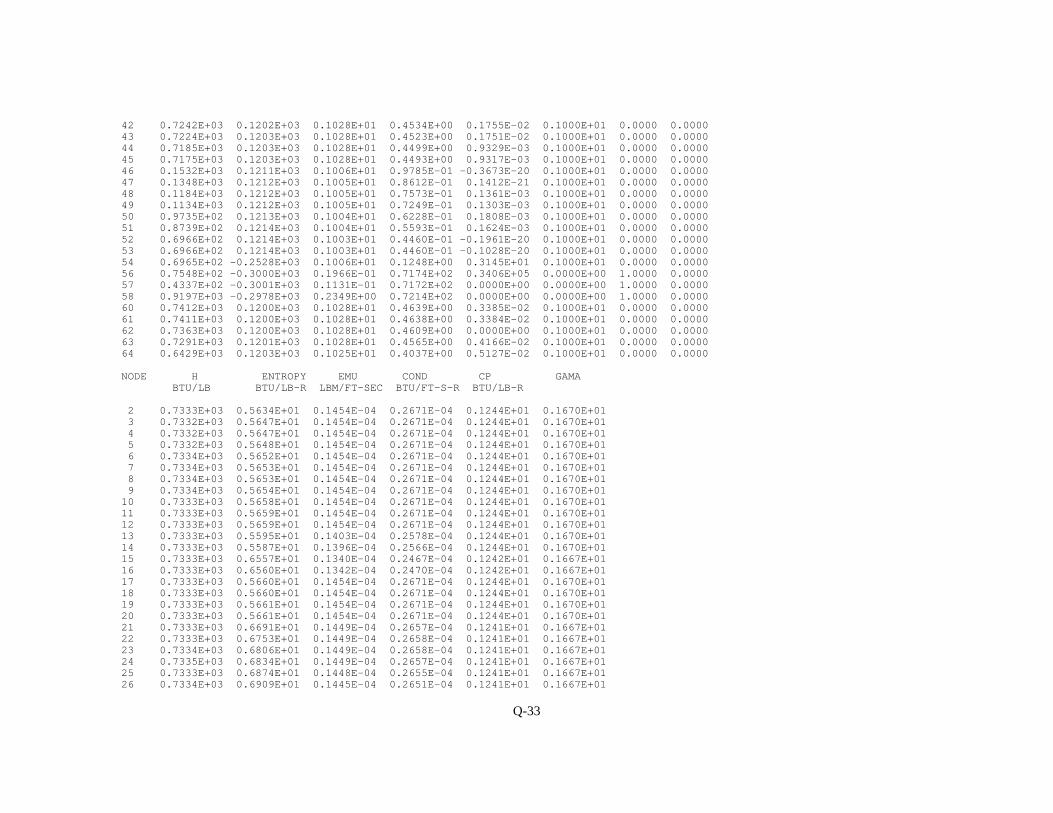


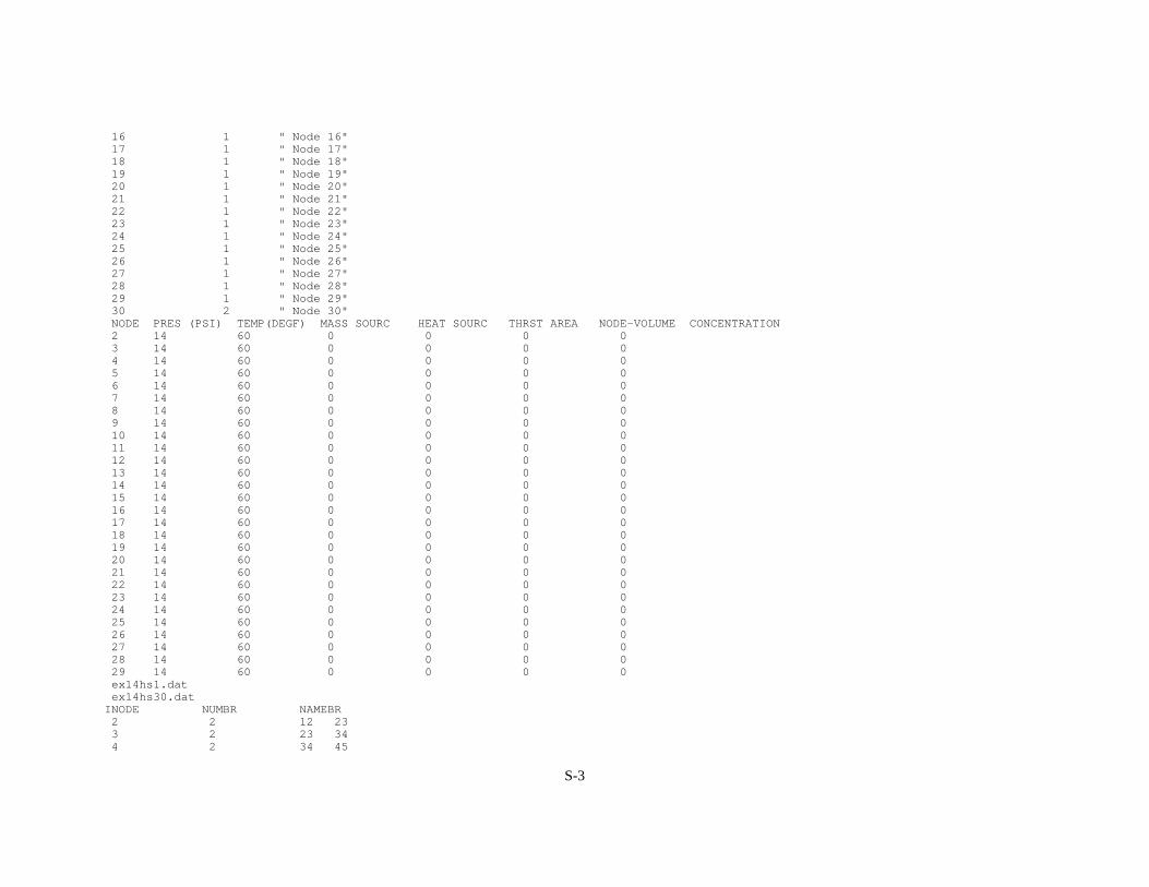


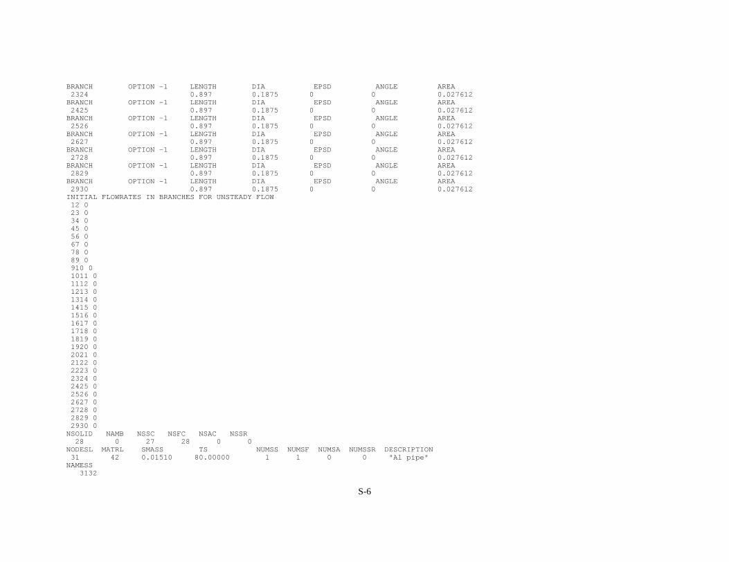
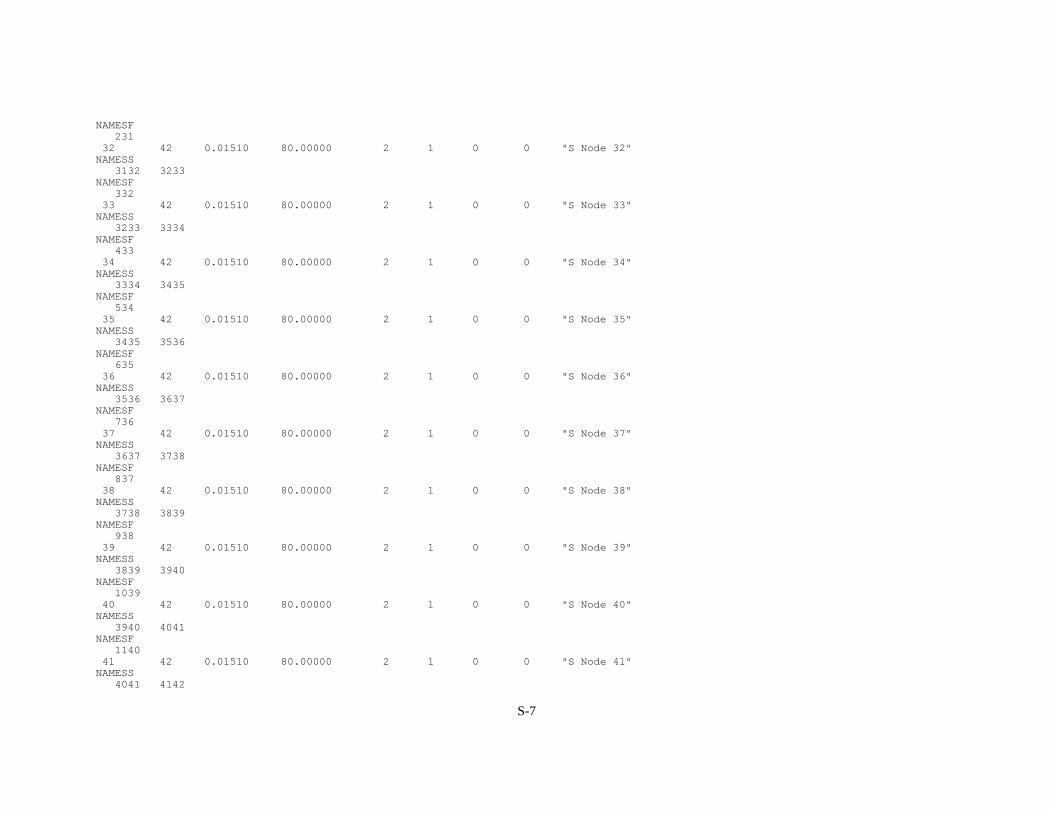
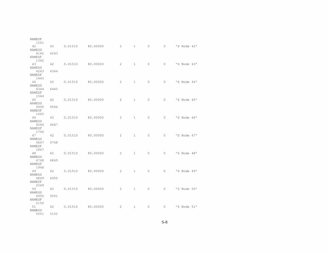

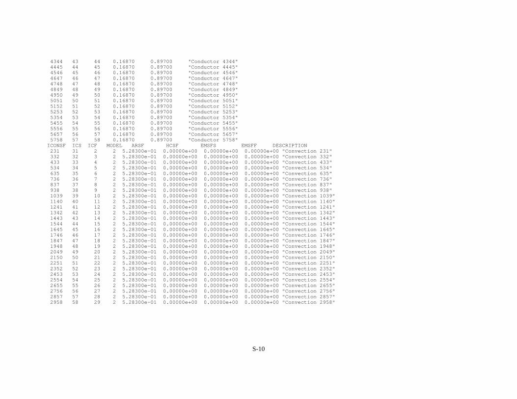

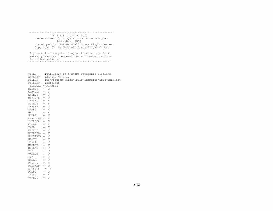

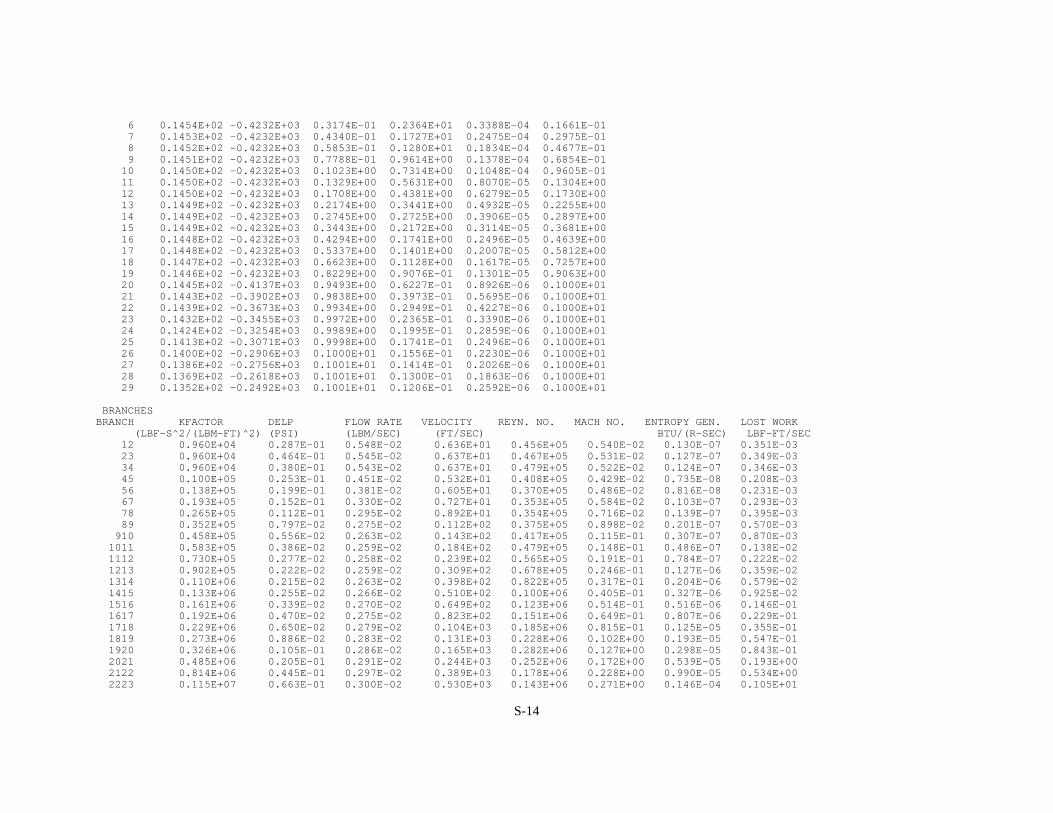
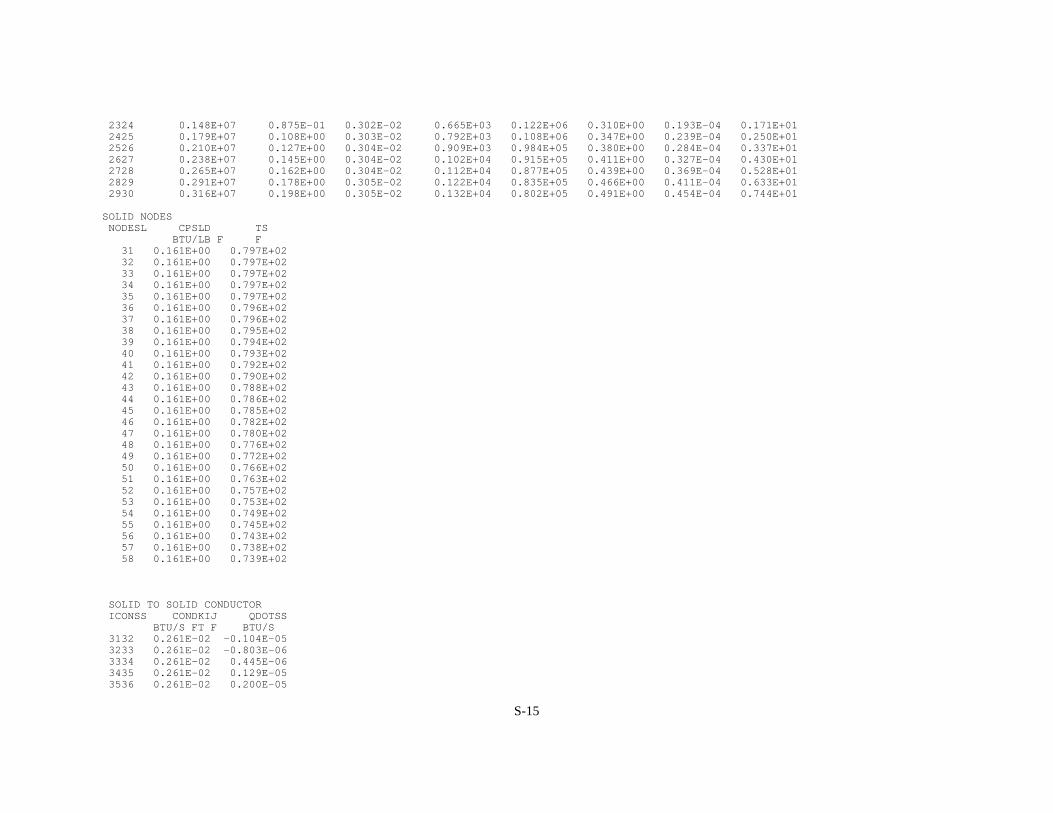


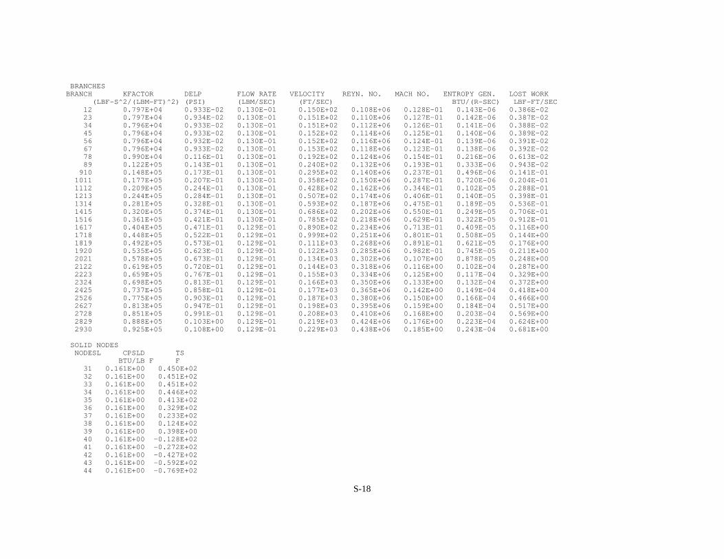

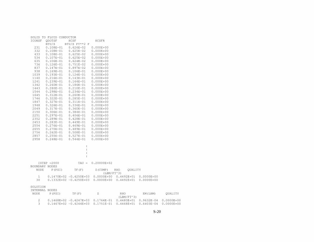
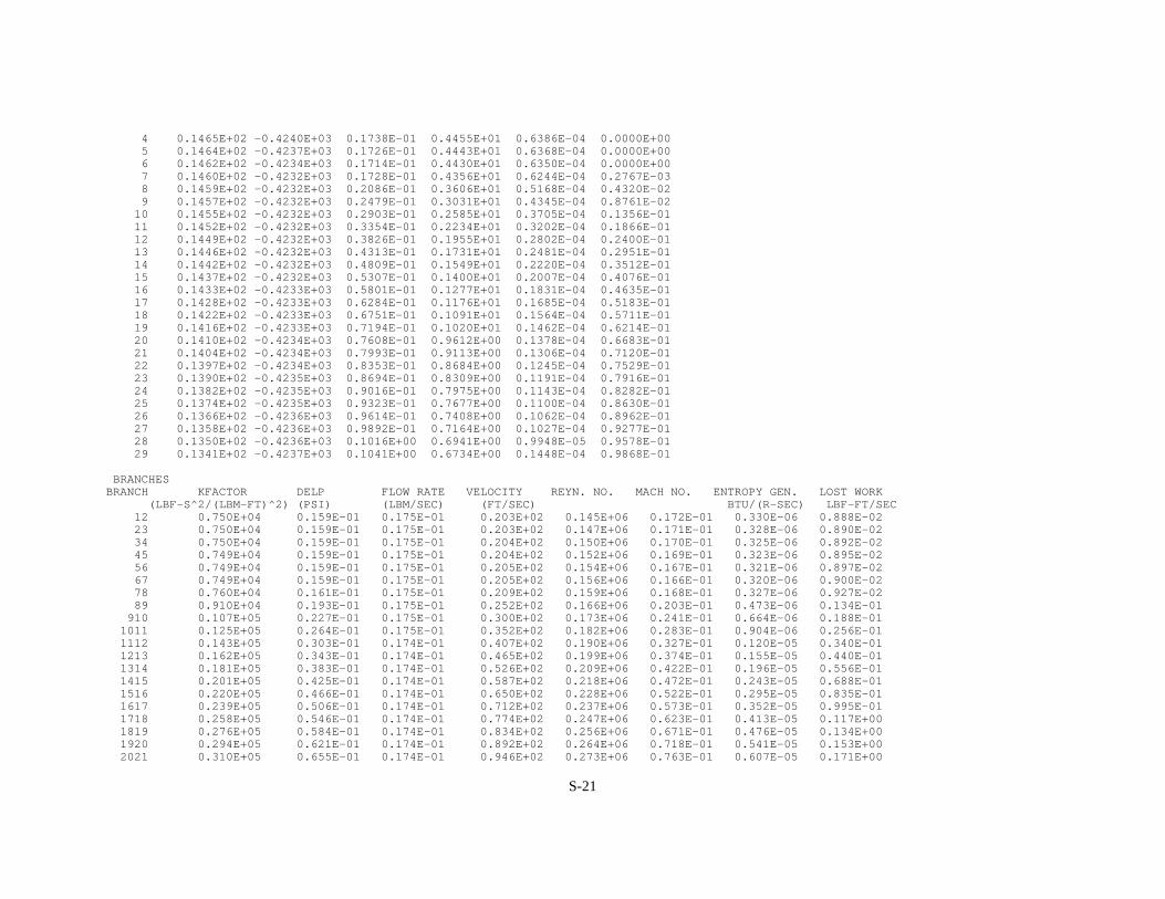
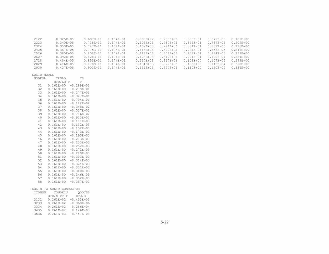
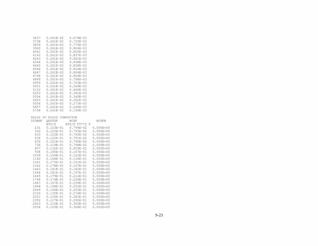


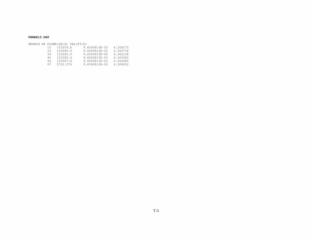


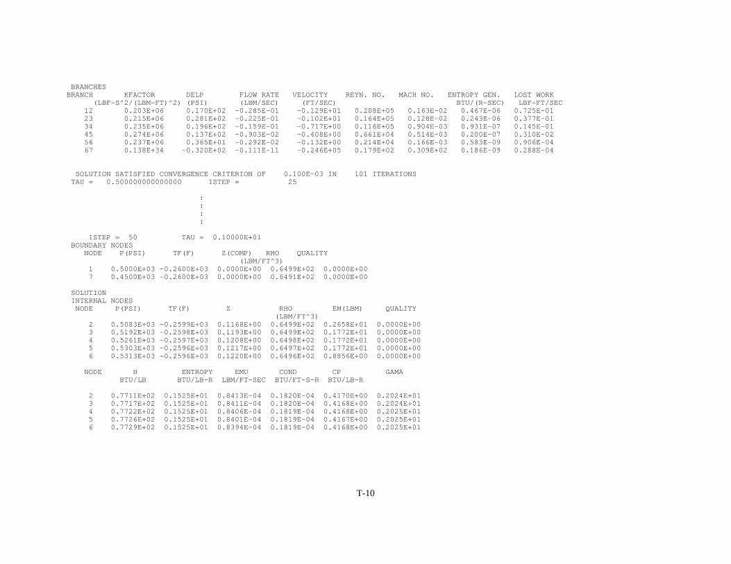


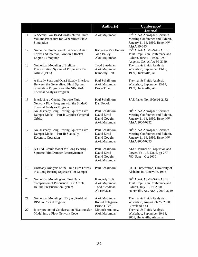
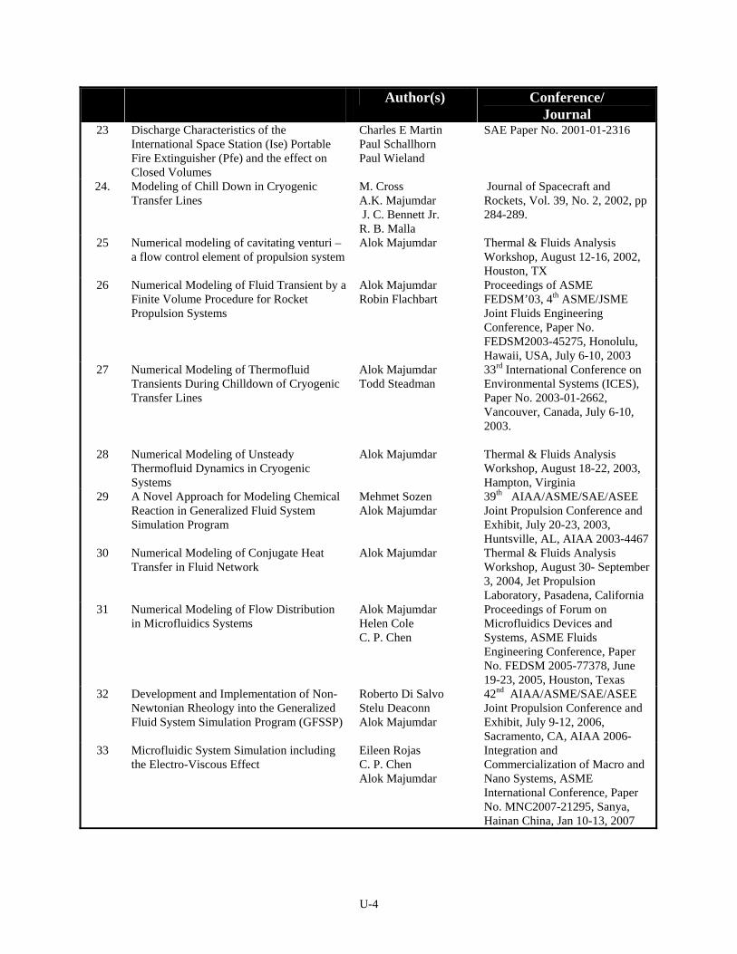


![GENERALIZED UNSOLID AND GENERALIZED FLUID VARIETIES OF ...scientificadvances.co.in/admin/img_data/180/images/[5] JPAMAA 010105... · 66 SARAWUT PHUAPONG and SORASAK LEERATANAVALEE](https://static.documents.pub/doc/80x56/5e0ab55c7c5ef967af1ade35/generalized-unsolid-and-generalized-fluid-varieties-of-5-jpamaa-010105.jpg)


