Generalized Linear Failure Rate Distribution

Ammar M. Sarhana∗ and Debasis Kundub

a Department of Mathematics, Faculty of Science,Mansoura University, Mansoura 35516, Egypt.

asarhan0@yahoo.com

bDepartment of Mathematics and StatisticsIndian Institute of Technology Kanpur,

Kanpur, 208016, Indiakundu@iitk.ac.in

Abstract

The exponential and Rayleigh are the two most commonly used distributions foranalyzing lifetime data. These distributions have several desirable properties and nicephysical interpretations. Unfortunately the exponential distribution only has constantfailure rate and the Rayleigh distribution has increasing failure rate. The linear failurerate distribution generalizes both these distributions which may have non-increasinghazard function also. This paper introduces a new distribution, which generalizesthe well known (1) exponential distribution, (2) linear failure rate distribution, (3)generalized exponential distribution, and (4) generalized Rayleigh distribution. Theproperties of this distribution are discussed in this paper. The maximum likelihoodestimates of the unknown parameters are obtained. A real data set is analyzed and itis observed that the present distribution can provide a better fit than some other verywell known distributions.

Key Words: Linear failure rate distribution, generalized exponential distribution, gener-

alized Rayleigh distribution, maximum likelihood method.

∗Current address: Department of Statistics and O.R., Faculty of Science, King Saud University, P.O. Box2455, Riyadh 11451, Saudi Arabia. E-mail: asarhan@ksu.edu.sa

1

1 Introduction

In analyzing lifetime data one often uses the exponential, Rayleigh, linear failure rate or gen-

eralized exponential distributions. It is well known that exponential can have only constant

hazard function whereas Rayleigh, linear failure rate and generalized exponential distribution

can have only monotone (increasing in case of Rayleigh or linear failure rate and increasing/

decreasing in case of generalized exponential distribution) hazard functions. Unfortunately,

in practice often one needs to consider non-monotonic function such as bathtub shaped haz-

ard function also, see, for example, Lai et al. [14]. In this paper we present a new simple

distribution which may have bathtub shaped hazard function and it generalizes many well

known distributions including the traditional linear failure rate distribution.

The linear failure rate distribution with the parameters a > 0 and b > 0, will be denoted

by LFRD(a, b), has the following cumulative distribution function (CDF)

FLF (x; a, b) = 1− exp{

−ax− b

2x2

}

, x ≥ 0. (1)

It is easily observed that the exponential distribution (ED(a)) and the Rayleigh distribution

(RD(b)) can be obtained from LFRD(a, b) by putting b = 0 and a = 0 respectively. Moreover,

the probability density function (PDF) of the LFRD(a, b) can be decreasing or unimodal but

the failure rate function is either constant or increasing only. See for example Bain [2], Sen

and Bhattacharya [19], Lin et al. [16], Ghitany and Kotz [9] and the references cited their

in this connection.

Recently, the two-parameter generalized exponential (GE) distribution has been intro-

duced and studied quite extensively by Gupta and Kundu [11]. The two-parameter GE

distribution with the parameters a > 0, θ > 0, has the following distribution function

FGE(x; a, θ) =(

1− e−ax)θ; x ≥ 0. (2)

It is observed that the GE(a, θ) can have decreasing or unimodal PDF and monotone (in-

creasing/ decreasing) hazard functions, depending on the shape parameter θ. Unfortunately,

2

it can not have bathtub shaped hazard function. Surles and Padgett [20] recently introduced

two-parameter Burr Type X distribution, also known as the generalized Rayleigh distribu-

tion, has increasing or bathtub shaped hazard function but it can not have decreasing hazard

function.

In this paper we introduce a new three-parameter distribution function called as gener-

alized linear failure rate distribution with three parameters a, b, θ and it will be denoted as

GLFRD(a, b, θ). It is observed that the new distribution has decreasing or unimodal PDF

and it can have increasing, decreasing and bathtub shaped hazard functions. We provide

different statistical properties of this new distribution and some nice physical interpretations

also. We provide the maximum likelihood estimates (MLEs) of the unknown parameters and

it is observed that they can not be obtained in explicit forms. The MLEs can be obtained

only by solving two non-linear equations. We analyze one real data set and it is observed

that the present distribution provides better fit than many existing well known distributions.

The rest of the paper is organized as follows. In section 2 we present GLFRD(a, b, θ) and

discuss its properties in Section 3. Section 4 discusses the distribution of order statistics of

the GLFRD. The MLEs are provided in Section 5. Section 6 gives an illustrative example to

explain how a real data set can be modeled by GLFRD(a, b, θ) and finally we conclude the

paper in Section 7. A list of acronyms are provided in the Appendix A for quick references.

2 The GLFRD

Let X be a random variable with the following CDF for a > 0, b > 0 and θ > 0 as follows;

F (x; a, b, θ) =[

1− e−(ax+ b2x2)]θ

, x ≥ 0. (3)

Here θ is shape parameter. The distribution of this form is said to be a generalized linear

failure rate distribution with parameters a, b, θ and will be denoted by GLFRD(a, b, θ). The

PDF and the hazard function of GLFRD(a, b, θ) will be

f(x; a, b, θ) = θ(a+ bx)[

1− e−(ax+ b2x2)]θ−1

e−(ax+ b2x2), x ≥ 0, (4)

3

and

h(x; a, b, θ) =θ(a+ bx)

[

1− e−(ax+ b2x2)]θ−1

e−(ax+ b2x2)

1−[

1− e−(ax+ b2x2)]θ

, (5)

respectively. Recently, it is observed, see Gupta and Gupta [10], that the reversed hazard

function plays an important role in the reliability analysis. The reversed hazard function of

the GLFRD(a, b, θ) is

r(x; a, b, θ) =f(x; a, b, θ)

F (x; a, b, θ)= θ(a+ bx)e−(ax+ b

2x2)

1− e−(ax+ b2x2)

= θf(x; a, b, 1)

F (x; a, b, 1)= θr(x; a, b, 1). (6)

It is well known that the hazard function or the reversed hazard function uniquely detrmines

the corresponding probabililty density function. From (6) it is clear that the GLFRD(a, b, θ)

is a proprtional reversed hazard family. It may be mentioned that the reversed hazard

function is a decreasing function.

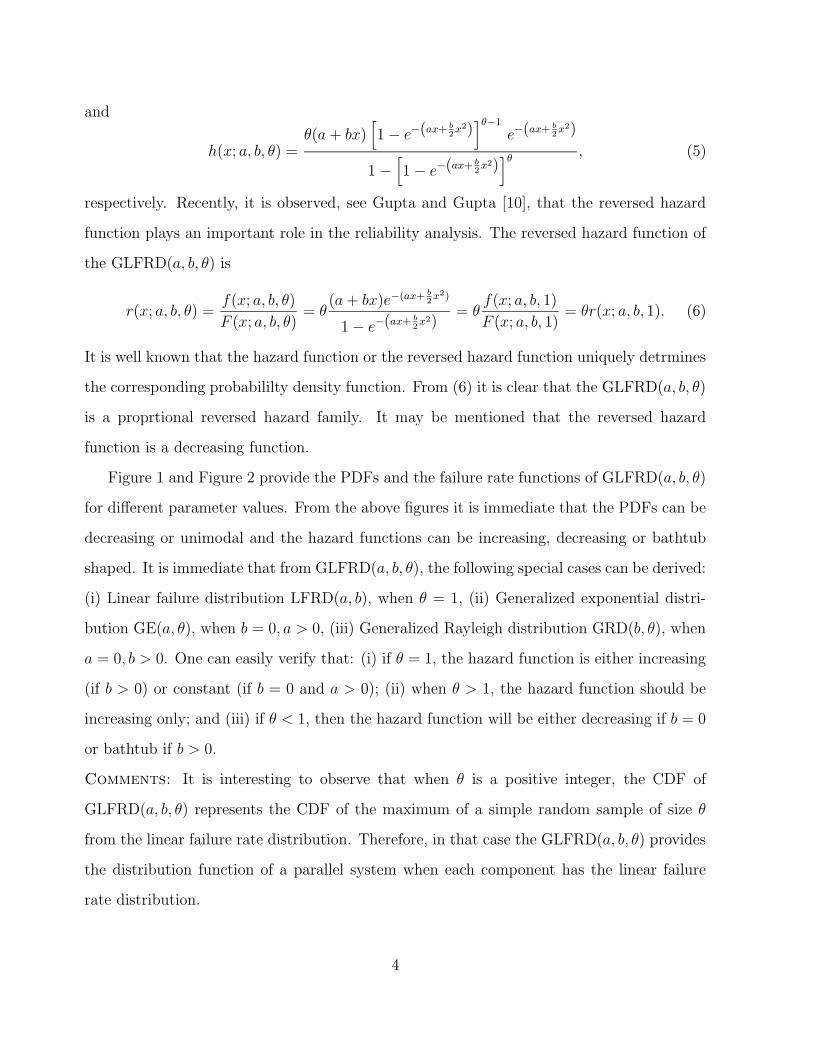
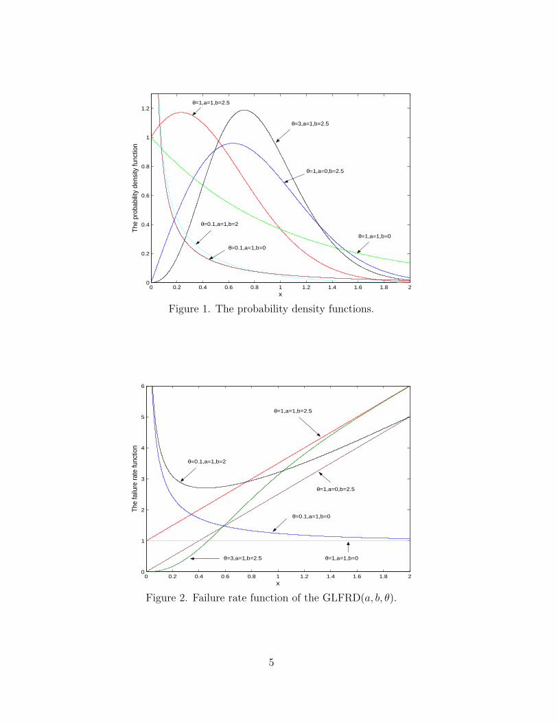
Figure 1 and Figure 2 provide the PDFs and the failure rate functions of GLFRD(a, b, θ)

for different parameter values. From the above figures it is immediate that the PDFs can be

decreasing or unimodal and the hazard functions can be increasing, decreasing or bathtub

shaped. It is immediate that from GLFRD(a, b, θ), the following special cases can be derived:

(i) Linear failure distribution LFRD(a, b), when θ = 1, (ii) Generalized exponential distri-

bution GE(a, θ), when b = 0, a > 0, (iii) Generalized Rayleigh distribution GRD(b, θ), when

a = 0, b > 0. One can easily verify that: (i) if θ = 1, the hazard function is either increasing

(if b > 0) or constant (if b = 0 and a > 0); (ii) when θ > 1, the hazard function should be

increasing only; and (iii) if θ < 1, then the hazard function will be either decreasing if b = 0

or bathtub if b > 0.

Comments: It is interesting to observe that when θ is a positive integer, the CDF of

GLFRD(a, b, θ) represents the CDF of the maximum of a simple random sample of size θ

from the linear failure rate distribution. Therefore, in that case the GLFRD(a, b, θ) provides

the distribution function of a parallel system when each component has the linear failure

rate distribution.

4

0 0.2 0.4 0.6 0.8 1 1.2 1.4 1.6 1.8 20

0.2

0.4

0.6

0.8

1

1.2

The

prob

abili

ty d

ensi

ty fu

nctio

n

x

θ=1,a=1,b=2.5

θ=1,a=0,b=2.5

θ=1,a=1,b=0

θ=3,a=1,b=2.5

θ=0.1,a=1,b=2

θ=0.1,a=1,b=0

Figure 1. The probability density functions.

0 0.2 0.4 0.6 0.8 1 1.2 1.4 1.6 1.8 20

1

2

3

4

5

6

The

failu

re ra

te fu

nctio

n

x

θ=1,a=1,b=2.5

θ=1,a=0,b=2.5

θ=1,a=1,b=0θ=3,a=1,b=2.5

θ=0.1,a=1,b=2

θ=0.1,a=1,b=0

Figure 2. Failure rate function of the GLFRD(a, b, θ).

5

3 Statistical properties

3.1 Mean, median and mode

It is observed as expected that the mean of the GLFRD(a, b, θ) can not be obtained in

explicit forms. It can be obtained as infinite series expansion. In general different moments

of the GLFRD(a, b, θ) will be presented later.

The quantile xq of the GLFRD(a, b, θ) is given by

xq =1

b

{

−a+√

a2 − 2b ln(

1− q1

θ

)

}

. (7)

Using (7), the median of GLFRD(a, b, θ) can be obtained as

med(X) =1

b

{

−a+√

a2 − 2b ln(

1− 2− 1

θ

)

}

. (8)

Moreover, the mode of GLFRD(a, b, θ) can be obtained as a solution of the following

non-linear equation

b− (a+ bx)2

a+ bx+ (θ − 1) (a+ bx)

exp{

ax+ b2x2}

− 1 = 0. (9)

It is not possible to obtain the explicit solution in the general case. It has to be obtained

numerically. For different special cases, the explicit forms may be obtained.

3.2 Moments

The following lemma gives the kth moment of GLFRD(a, b, θ), when θ ≥ 1.

Lemma 3.1 If X has GLFRD(a, b, θ), then the kth moment of X, say µ(k), is given as

follows

For a = 0, b > 0:

µ(k) =θ Γ(k

2+ 1)

(

b2

)k

∞∑

i=0

(−1)−i(θ−1i )

(i+ 1)k2+1

, (10)

For a > 0, b ≥ 0:

µ(k) = θ∞∑

i=0

∞∑

`=0

(−1)−i(θ−1i )Γ(k + `+ 1) g

(`)i (0)

`![a(i+ 1)]k+`+1

[

a+(k + `+ 1)b

(i+ 1)a

]

, (11)

6

θ

Sk

ewn

ess

0.5

0.6

0.7

0.8

0.9

1

1.1

1.2

1.3

1.4

1.5

0 1 2 3 4 5 6 7 8 9 10

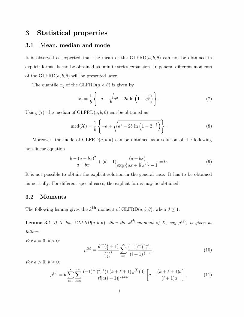
Figure 3. The skewness measure.

here g(`)i (0) =

d`

dx`exp{−1

2(i+ 1)bx2}

∣

∣

x=0and Γ(.) is the complete gamma function.

The proof of this lemma is provided in the Appendix B.

Based on the results, the measures of skewness and kurtosis of the GLFRD can be obtained

as respectively;

α =µ(3) − 3µµ(2) + 2µ3

(µ(2) − µ2)3

2

(12)

and

β =µ(4) − 4µµ(3) + 6µ2 µ(2) − 3µ4

(µ(2) − µ2)2 . (13)

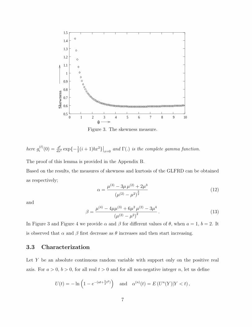
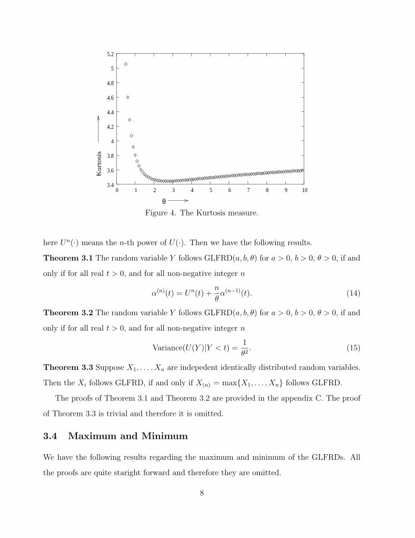
In Figure 3 and Figure 4 we provide α and β for different values of θ, when a = 1, b = 2. It

is observed that α and β first decrease as θ increases and then start increasing.

3.3 Characterization

Let Y be an absolute continuous random variable with support only on the positive real

axis. For a > 0, b > 0, for all real t > 0 and for all non-negative integer n, let us define

U(t) = − ln(

1− e−(at+ b2t2))

and α(n)(t) = E (Un(Y )|Y < t) ,

7

θ

Kurt

osi

s

3.4

3.6

3.8

4

4.2

4.4

4.6

4.8

5

5.2

0 1 2 3 4 5 6 7 8 9 10

Figure 4. The Kurtosis measure.

here Un(·) means the n-th power of U(·). Then we have the following results.

Theorem 3.1 The random variable Y follows GLFRD(a, b, θ) for a > 0, b > 0, θ > 0, if and

only if for all real t > 0, and for all non-negative integer n

α(n)(t) = Un(t) +n

θα(n−1)(t). (14)

Theorem 3.2 The random variable Y follows GLFRD(a, b, θ) for a > 0, b > 0, θ > 0, if and

only if for all real t > 0, and for all non-negative integer n

Variance(U(Y )|Y < t) =1

θ2. (15)

Theorem 3.3 Suppose X1, . . . , Xn are indepedent identically distributed random variables.

Then the Xi follows GLFRD, if and only if X(n) = max{X1, . . . , Xn} follows GLFRD.

The proofs of Theorem 3.1 and Theorem 3.2 are provided in the appendix C. The proof

of Theorem 3.3 is trivial and therefore it is omitted.

3.4 Maximum and Minimum

We have the following results regarding the maximum and minimum of the GLFRDs. All

the proofs are quite staright forward and therefore they are omitted.

8

Theorem 3.4: IfXis are independent random variables, and supposeXi follows GLFRD(a, b, θi)

for i = 1, . . . , n, then X(n) follows GLFRD(a, b,n∑

i=1

θi)

Theorem 3.5: If Xis are independent and identically distributed random variables and Xi

follows GLFRD(a, b, θ), then for all −∞ < x <∞

limn→∞

P

(

X(n) − bnan

≤ x

)

= e−e−bβx ,

here bn =−2a+

√4a2 + 8 lnn

2band an is such that it satisfies the following two conditions;

limn→∞

an = 0, and limn→∞

anbn = β.

Theorem 3.6: If Xis are independent and identically distributed random variables and Xi

follows GLFRD(a, b, θ), then for X(1) = min{X1, . . . , Xn} and for all x > 0

limn→∞

P

(

X(1)

cn≤ x

)

= 1− e−(ax)θ ,

where cn = n−1

θ .

4 Distribution of order statistics

Let X1, X2, . . . , Xn be a simple random sample from GLFRD(a, b, θ) with PDF and CDF

as in (4) and (3), respectively. Let X(1) ≤ X(2) ≤ . . . ≤ X(n) denote the order statistics

obtained from this sample. In this section we provide the expressions for the PDFs and

moments of order statistics for the GLFRD(a, b, θ). Also, the measures of skewness and

kurtosis of the distribution of the rth order statistic are presented. The PDF of X(r) is given

by,

fr:n(x) =1

B(r, n− r + 1)[F (x; a, b, θ)]r−1 [1− F (x; a, b, θ)]n−r f(x; a, b, θ) , (16)

where f(x; a, b, θ), F (x; a, b, θ) are the PDF and CDF given by (4) and (3), respectively.

fr:n(x) =1

B(r, n− r + 1)f(x; a, b, θ)

n−r∑

j=0

(n−rj )(−1)j[F (x; a, b, θ)]r+j−1 (17)

9

substituting from (3) and (3) into (17), one gets

fr:n(x) =n−r∑

j=0

dj(n, r) f(x; a, b, θr+j), (18)

where

θi = iθ, dj(n, r) =n (−1)j (n−r

j ) (n−1r−1 )

(r + j).

The coefficients dj(n, r), j = 1, 2, . . . , n − r do not depend on a, b, θ. Thus fr:n(x) is the

weighted average of the generalized linear failure rate distributions with different shape

parameters.

Theorem 4.1 The kth moment of order statistic X(r) is

(i) if a = 0, b > 0:

µ(k)r:n = θ

(

2

b

) k2+1

Γ

(

k

2+ 1

) n−r∑

j=0

∞∑

i=0

d∗j(n, r)(−1)i (θr+j−1

i )

(i+ 1)k2+1

. (19)

(ii) if a > 0, b ≥ 0:

µ(k)r:n = θ

n−r∑

j=0

∞∑

i=0

∞∑

`=0

d∗j(n, r)(−1)i (θr+j−1

i ) g(`)i Γ(k + `+ 1)

`! [(i+ 1)a]k+`+1

[

a+(k + `+ 1)b

(i+ 1)a

]

, (20)

here d∗j(n, r) = (r + j) dj(n, r).

The proof of this Theorem is given in the Appendix B.

Based on the results given in theorem (4.1), the measures of skewness and kurtosis of the

distribution of the rth order statistic can be evaluated from the following expressions

αr:n =µ

(3)r:n − 3µr:n µ

(2)r:n + 2µ3

r:n(

µ(2)r:n − µ2

r:n

) 3

2

(21)

and

βr:n =µ

(4)r:n − 4µ(3)

r:n + 6µ2r:n µ

(2)r:n − 3µ4

r:n(

µ(2)r:n − µ2

r:n

)2 . (22)

Extensive tables are available on request from the authors for different values of αr:n and

βr:n for the cases in which n = 1, 2, 3, 4, 5 and θ = 0.5, 1, 1.5, 2, 2.5, 3, 3.5 with 1 ≤ r ≤ n.

From the table values the general findings are (i) The distribution of the rth order statistic

is positively skewed. (ii) For fixed θ and n, the values of βr:n increases as r increases.

10

5 Parameter estimations

In this section, we derive the maximum likelihood estimates of the unknown parameters

a, b, θ of GLFRD(a, b, θ) based on a complete sample. Let us assume that we have a simple

random sample X1, X2, · · · , Xn from GLFRD(a, b, θ). The likelihood function of this sample

is

L =n∏

i=1

f(xi; a, b, θ). (23)

Substituting from (4) into (23), we get

L =n∏

i=1

{

θ(a+ bxi)[

1− e−(axi+b2x2i )]θ−1

e−(axi+b2x2i )}

. (24)

It can be written as;

L = θn exp {−aT1 − bT2}n∏

i=1

{

(a+ bxi)[

1− e−(axi+b2x2i )]θ−1

}

, (25)

where Tj =1

j

n∑

i=1

xji , j = 1, 2.

The log-likelihood function becomes

L = n ln θ − aT1 − bT2 +n∑

i=1

ln(a+ bxi) + (θ − 1)n∑

i=1

ln[

1− e−(axi+b2x2i )]

. (26)

Therefore, the normal equations are

∂L∂a

= −T1 +n∑

i=1

1

a+ bxi+ (θ − 1)

n∑

i=1

xie−(axi+ b

2x2i )

1− e−(axi+b2x2i )= 0, (27)

∂L∂b

= −T2 +n∑

i=1

xia+ bxi

+1

2(θ − 1)

n∑

i=1

x2i e

−(axi+ b2x2i )

1− e−(axi+b2x2i )= 0, (28)

∂L∂θ

=n

θ+

n∑

i=1

ln[

1− e−(axi+b2x2i )]

= 0. (29)

The normal equations do not have explicit solutions and they have to be obtained numeri-

cally. Note that for a given a and b, the MLE of θ, say θ(a, b) can be obtained as

θ(a, b) = − n∑n

i=1 ln[

1− e−(axi+b2x2i )] .

Therefore, the MLEs of a and b can be obtained by solving two non-linear equations.

11

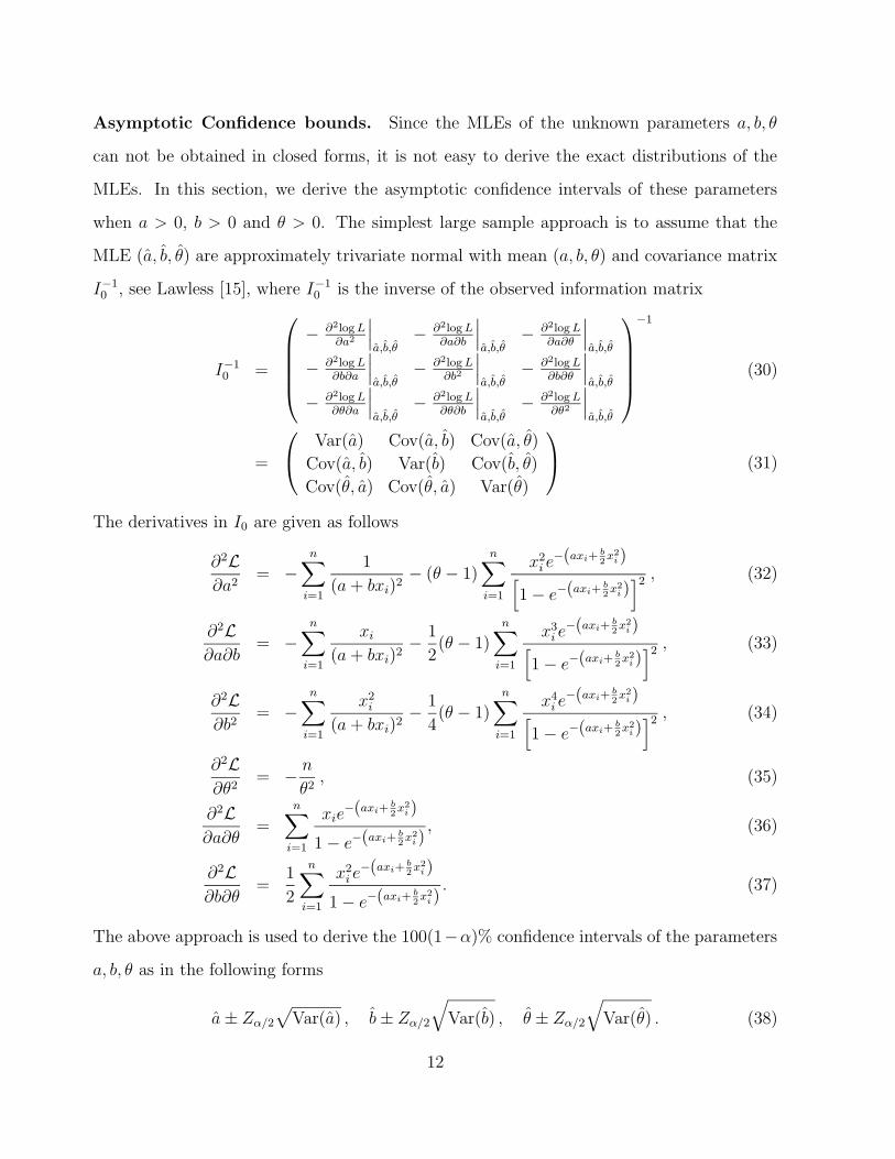
Asymptotic Confidence bounds. Since the MLEs of the unknown parameters a, b, θ

can not be obtained in closed forms, it is not easy to derive the exact distributions of the

MLEs. In this section, we derive the asymptotic confidence intervals of these parameters

when a > 0, b > 0 and θ > 0. The simplest large sample approach is to assume that the

MLE (a, b, θ) are approximately trivariate normal with mean (a, b, θ) and covariance matrix

I−10 , see Lawless [15], where I

−10 is the inverse of the observed information matrix

I−10 =

− ∂2logL∂a2

∣

∣

∣

a,b,θ− ∂2logL

∂a∂b

∣

∣

∣

a,b,θ− ∂2logL

∂a∂θ

∣

∣

∣

a,b,θ

− ∂2logL∂b∂a

∣

∣

∣

a,b,θ− ∂2logL

∂b2

∣

∣

∣

a,b,θ− ∂2logL

∂b∂θ

∣

∣

∣

a,b,θ

− ∂2logL∂θ∂a

∣

∣

∣

a,b,θ− ∂2logL

∂θ∂b

∣

∣

∣

a,b,θ− ∂2logL

∂θ2

∣

∣

∣

a,b,θ

−1

(30)

=

Var(a) Cov(a, b) Cov(a, θ)

Cov(a, b) Var(b) Cov(b, θ)

Cov(θ, a) Cov(θ, a) Var(θ)

(31)

The derivatives in I0 are given as follows

∂2L∂a2

= −n∑

i=1

1

(a+ bxi)2− (θ − 1)

n∑

i=1

x2i e

−(axi+ b2x2i )

[

1− e−(axi+b2x2i )]2 , (32)

∂2L∂a∂b

= −n∑

i=1

xi(a+ bxi)2

− 12(θ − 1)

n∑

i=1

x3i e

−(axi+ b2x2i )

[

1− e−(axi+b2x2i )]2 , (33)

∂2L∂b2

= −n∑

i=1

x2i

(a+ bxi)2− 14(θ − 1)

n∑

i=1

x4i e

−(axi+ b2x2i )

[

1− e−(axi+b2x2i )]2 , (34)

∂2L∂θ2

= − n

θ2, (35)

∂2L∂a∂θ

=n∑

i=1

xie−(axi+ b

2x2i )

1− e−(axi+b2x2i ), (36)

∂2L∂b∂θ

=1

2

n∑

i=1

x2i e

−(axi+ b2x2i )

1− e−(axi+b2x2i ). (37)

The above approach is used to derive the 100(1−α)% confidence intervals of the parameters

a, b, θ as in the following forms

a± Zα/2

√

Var(a) , b± Zα/2

√

Var(b) , θ ± Zα/2

√

Var(θ) . (38)

12

Here, Zα/2 is the upper (α/2)th percentile of the standard normal distribution.

It should be mentioned here as it was pointed by a referee that if we do not make the

assumption that the true parameter vector (a, b, θ) is an interior point of the parameter

space then the asymptotic normality results will not hold. If any of the true parameter value

is 0, then the asymptotic distribution of the maximum likelihood estimators is a mixture

distribution, see for example Self and Liang [18] in this connection. In that case obtaining

the asymptotic confidence intervals become quite difficult and it is not pursued here.

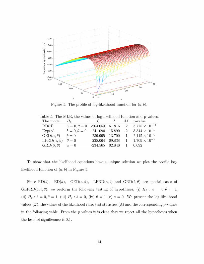
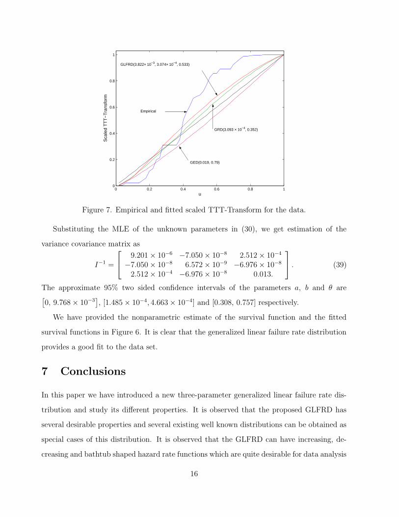
6 Data Analysis

In this section we provide a data analysis to see how the new model works in practice. The

data have been obtained from Aarset [1] and it is provided below. It represents the lifetimes

of 50 devices.

.1 .2 1 1 1 1 1 2 3 6 7 11 12 18 18 18 18 1821 32 36 40 45 46 47 50 55 60 63 63 67 67 67 67 72 7579 82 82 83 84 84 84 85 85 85 85 85 86 86

We have used different distributions namely; Rayleigh distribution (RD), exponential dis-

tribution (ED), generalized exponential distribution (GED), linear failure rate distribution

(LFRD), generalized Rayleigh distribution (GRD) and generalized linear failure rate distri-

bution (GLFRD) to analyze the data. The MLE(s) of the unknown parameter(s) and the

corresponding Kolmogorov-Smirnov (K-S) test statistic for 6 different models are given in

Table 4.

Table 4. The MLE of the parameter(s) and the associated K-S values.The model MLE of the parameter(s) K-S

RD(b) b = 6.362× 10−4 0.315ED(a) a = 0.022 0.171

GED(a, θ) a = 0.019, θ = 0.78 0.184

LFRD(a, b) a = 0.014, b = 2.4× 10−4 0.195

GRD(b, θ) b = 3.093× 10−4, θ = 0.352 0.181

GLFRD(a, b, θ) a = 3.822× 10−3, b = 3.074× 10−4, θ = 0.533 0.162

13

0

10

20

30

40

0

50

100

150

200−340

−320

−300

−280

−260

−240

−220

ab

The

prof

ile o

f log

−lik

elih

ood

func

tion

Figure 5. The profile of log-likelihood function for (a, b).

Table 5. The MLE, the values of log-likelihood function and p-values.The model H0 L Λ d.f. p-valueRD(β) a = 0, θ = 0 -264.053 61.816 2 3.775× 10−14

Exp(α) b = 0, θ = 0 -241.090 15.890 2 3.544× 10−4

GED(α, θ) b = 0 -239.995 13.700 1 2.145× 10−4

LFRD(α, β) θ = 0 -238.064 09.838 1 1.709× 10−3

GRD(β, θ) a = 0 -234.565 02.840 1 0.092

To show that the likelihood equations have a unique solution we plot the profile log-

likelihood function of (a, b) in Figure 5.

Since RD(b), ED(a), GED(a, θ), LFRD(a, b) and GRD(b, θ) are special cases of

GLFRD(a, b, θ), we perform the following testing of hypotheses; (i) H0 : a = 0, θ = 1,

(ii) H0 : b = 0, θ = 1, (iii) H0 : b = 0, (iv) θ = 1 (v) a = 0. We present the log-likelihood

values (L), the values of the likelihood ratio test statistics (Λ) and the corresponding p-values

in the following table. From the p values it is clear that we reject all the hypotheses when

the level of significance is 0.1.

14

0 10 20 30 40 50 60 70 80 900

0.1

0.2

0.3

0.4

0.5

0.6

0.7

0.8

0.9

1

Surv

ival

func

tion

x

RD

ED

GRD

GED

GLFRD

K−M

LFRD

Figure 6. The Kaplan-Meier estimate of survival function and fitted survival functions.

For the comparison purpose, the empirical and fitted total time on test transforms (TTT-

Transforms) using the GLFRD, GRD and GED are provided. For details about the TTT-

Transform technique, we refer to [3], [5] and [6]. Figure 7 shows the plots of the empirical

and fitted TTT-Transform of the data. Further, we computed: (i) the maximum of the

distance between the fitted TTT-transform using each distribution and the empirical one;

(ii) the mean squared error of the fitted TTT-Transforms using each suggested distribution.

Table 6 gives the obtained results.

Table 6: The distance of the TTT-Transform.Distribution Maximum distance MSEGED 0.3332 0.0348GRD 0.2286 0.0149GLFRD 0.1940 0.0112

15

0 0.2 0.4 0.6 0.8 10

0.2

0.4

0.6

0.8

1

u

Sca

led

TT

T−

Tra

nsfo

rm

GED(0.019, 0.79)

GRD(3.093 × 10−4, 0.352)

GLFRD(3.822× 10−3, 3.074× 10−4, 0.533)

Empirical

Figure 7. Empirical and fitted scaled TTT-Transform for the data.

Substituting the MLE of the unknown parameters in (30), we get estimation of the

variance covariance matrix as

I−1 =

9.201× 10−6 −7.050× 10−8 2.512× 10−4

−7.050× 10−8 6.572× 10−9 −6.976× 10−8

2.512× 10−4 −6.976× 10−8 0.013.

. (39)

The approximate 95% two sided confidence intervals of the parameters a, b and θ are[

0, 9.768× 10−3]

, [1.485× 10−4, 4.663× 10−4] and [0.308, 0.757] respectively.

We have provided the nonparametric estimate of the survival function and the fitted

survival functions in Figure 6. It is clear that the generalized linear failure rate distribution

provides a good fit to the data set.

7 Conclusions

In this paper we have introduced a new three-parameter generalized linear failure rate dis-

tribution and study its different properties. It is observed that the proposed GLFRD has

several desirable properties and several existing well known distributions can be obtained as

special cases of this distribution. It is observed that the GLFRD can have increasing, de-

creasing and bathtub shaped hazard rate functions which are quite desirable for data analysis

16

purposes. We obtained the asymptotic properties of the MLEs of the unknown parameters

but we have not studied the behavior of the MLEs for small sample sizes. Extensive simula-

tions are required to study the rate of convergence of the MLEs and their various properties.

More work is needed in this direction.

Acknowledgements

The authors would like to thank two referees and the associate editor for many constructive

suggestions.

Appendix A

Acronyms:

LFRD: Linear failure rate distribution

CDF: Cumulative distribution function

ED: Exponential distribution

RD: Rayleigh distribution

PDF: Probabibility density function

CDF: Cumulative distribution function

GE: Generalized exponential distribution

MLEs: Maximum likelihood estimators

GLFRD: Generalized failure rate distribution

Appendix B

The Proof of Lemma 3.1. Starting with

µ(k) =

∫ ∞

0

xkf(x; a, b, θ)dx

17

then substituting from (4) into the above relation we have

µ(k) = θ

∫ ∞

0

xk(a+ bx)[

1− e−(ax+ b2x2)]θ−1

e−(ax+ b2x2)dx.

Since 0 < e−(ax+ b2x2) < 1 for x > 0, by using the binomial series expansion we have

[

1− e−(ax+ b2x2)]θ−1

=∞∑

i=0

(−1)i(θ−1i ) e

−i(ax+ b2x2), (40)

then

µ(k) = θ

∫ ∞

0

xk(a+ bx)∞∑

i=0

(−1)i(θ−1i ) e

−(i+1)(ax+ b2x2)dx. (41)

Since the inner quantity of the summation is absolutely integrable, interchanging the inte-

gration and summation we get

µ(k) = θ

∞∑

i=0

(−1)i(θ−1i )

∫ ∞

0

xk(a+ bx) e−(i+1)(ax+ b2x2)dx. (42)

Now arises two cases. The first case arises when a = 0 and b > 0. In this case, the integral

in (42) becomes

∫ ∞

0

xk(a+ bx) e−(i+1)(ax+ b2x2)dx =

∫ ∞

0

bxk+1 e−b2

(i+1)x2

dx =b

2

Γ(k2+ 1)

[ b2(i+ 1)]

k2+1. (43)

Substituting from (43) into (42), one gets (10) which completes the first part of the lemma.

The second case arises when a > 0 and b ≥ 0. For this case, using the Taylor expansion of

the function e−b2(i+1)x2

given by

e−b2(i+1)x2

=∞∑

`=0

g(`)i (0)

`!x`, g

(`)i (0) =

d`

dx`e−

b2(i+1)x2|x=0,

one can rewrite (42) as

µ(k) = θ∞∑

i=0

∞∑

`=0

(−1)i(θ−1i )

g(`)i (0)

`!

∫ ∞

0

xk+`(a+ bx) e−(i+1)axdx

= θ

∞∑

i=0

∞∑

`=0

(−1)i(θ−1i )

g(`)i (0)

`!

[

aΓ(k + `+ 1)

[(i+ 1) a]k+`+1+

bΓ(k + `+ 2)

[(i+ 1) a]k+`+2

]

.

That completes the proof of the lemma.

18

The Proof of Theorem 4.1. The general definition of the kth moment of order statistic

X(r), is

µ(k)r:n =

∫ ∞

0

xkfr:n(x)dx. (44)

Substituting from (18) into (44), one gets

µ(k)r:n =

n−r∑

j=0

dj(n, r)

∫ ∞

0

xkf(x; a, b, θr+j) dx. (45)

Since the integral in (45) is the kth moment of GLFRD(a, b, θr+j), then from (45) with the

help of lemma (3.1) we get (19) and (20) which completes the proof.

Appendix C

Proof of Theorem 3.1

Necessary Part: If Y follows GLFRD(a, b, θ), then (14) follows using integration by parts

from the expresion of α(n)(t).

Sufficient Part: Suppose (14) is true for the random variable Y . Let us denote the PDF and

CDF of Y as fY (·) and FY (·) respectively. From (14) we obtain∫ t

0

Un(t)fY (y)dy = Un(t)FY (t) +n

θ

∫ t

0

Un−1(t)fY (y)dy. (46)

Differentiating (46) with respect to t, we obtain

Un(t)fY (t) = Un(t)fY (t)− nUn−1(t)FY (t)f(t; a, b, 1)

F (t; a, b, 1)+n

θUn−1(t)fY (t). (47)

Since Un−1(t) 6= 0, from (47) we obtain

fY (t)

FY (t)= θ

f(t; a, b, 1)

F (t; a.b, 1). (48)

From the uniqueness property of the reversed hazard function and from (6), it is immediate

that fY (x) has to be of the form (4).

Proof of Theorem 3.2

19

Necessary Part: Suppose Y follows GLFRD(a, b, θ), then from Theorem 3.1, we get

α(1)(t) = U(t) +1

θ(49)

and

α(2)(t) = U 2(t) +2

θα(1)(t) = U 2(t) +

2

θ

[

U(t) +1

θ

]

=(

α(1)(t))2+1

θ2. (50)

Therefore, the result follows.

Sufficient Part: Suppose (15) is true for all t > 0 for the random variable Y . Let us denote

the PDF and CDF of Y as fY (·) and FY (·) respectively. Therefore, (15) can be written as

FY (t)

∫ t

0

U2(y)fY (y)dy −[∫ t

0

U(y)fY (y)dy

]2

=F 2(y)

θ2. (51)

Differentiating both sides of (51) with respect to t and cancelling fY (t) from both sides, we

get∫ t

0

U2(y)fY (y)dy + FY (t)U2(t)− 2U(t)

∫ t

0

U(y)fY (y)dy = 2FY (t)

θ2. (52)

Differentiating both sides of (52) with respect to t and arranging terms, we obtain;

FY (t)U(t)−∫ t

0

U(y)fY (y)dy = −fY (t)

r(t; a, b, 1)θ2. (53)

After differentiating (53) with respect to t and rearranging we obtain the differential equation;

θ2FY (t) =1

r(t; a, b, 1)× d

dt

(

fY (t)

r(t; a, b, 1)

)

. (54)

A general solution of the differential equation (54) is of the form

FY (t) = c1eαU(t) + c2e

−αU(t),

where c1 and c2 are arbitrary constants. Since limt↓0

U(t) =∞ and limt→∞

U(t) = 0 and FY (t) is

a distribution function function, then c1 = 0 and c2 = 1. Therefore, the result follows.

References

[1] M. V. Aarset, “How to identify bathtub hazard rate,” IEEE Transactions on Reliability,

vol. R-36, 106 - 108, 1987.

20

[2] L. J. Bain, “Analysis for the Linear Failure-Rate Life-Testing Distribution,” Techno-

metrics, 16(4), 551 - 559, 1974.

[3] R. E. Barlow, R. Campo, “Total time on test processes and applications to failure data

analysis”, Reliability and Fault Tree Analysis (Barlow, Fussell, Singpurwalla, Eds), 451

- 481; SIAM, Philadelphia, 1975.

[4] R.E. Barlow and F. Proschan, Statistical Theory of Reliability and Life Testing. Prob-

ability Models. Holt, Rinehart & Winston, New York, 1975.

[5] B. Bergman, B. Klefsjo, “A graphical method applicable to agereplacement problems”,

IEEE Transactions on Reliability, vol R-31, 478 - 481, 1982.

[6] B. Bergman, B. Klefsjo, “The total time on test concept and its use in reliability theory”,

Operations Research, vol 32, 596 - 606, 1984.

[7] I.W. Burr, “Cumulative frequency function”, Annals of Mathematical Statistics, 13, 215

- 232, 1942.

[8] B.V. Genedenko, Y.K. Belyayev and A.D. Solovyev, Mathematical Methods of Relia-

bility Theory, Academic Press, New York, 1969.

[9] M.E. Ghitany, ”Reliability properties of extended linear failure-rate distributions”,

Probability in the Engineering and Information Sciences, vol. 21, 441 - 450, 2006.

[10] R.C. Gupta and R.D. Gupta, “Proportional reversed hazard model and its applications”,

Journal of Statistical Planning and Inference, vol. 137, no. 11, 3525 - 3536, 2007.

[11] R.D. Gupta and D. Kundu, “Generalized exponential distribution”, Austral. & New

Zealand Journal of Statistics, vol. 41, 173 - 188, 1999.

[12] D. Kundu and R.D. Gupta, “Characterization of the proportional (reversed) hazard

model”, Communications in Statistics - Theory and Methods, vol. 33, 3095 - 3102,

2004.

21

[13] D. Kundu and M. Raqab, “Generalized Rayleigh distribution: different methods of

estimations”, Computational Statistics & Data Analysis, vol. 49, 187 - 200, 2005.

[14] C. D. Lai, M. Xie, and D. N. P. Murthy, “Bathtub shaped failure rate distributions,”

in Handbook in Reliability, N. Balakrishnan and C. R. Rao, Eds., 20, 69 - 104, 2001.

[15] J. F. Lawless, “Statistical Models and Methods for Lifetime Data,” John Wiley and

Sons, New York, 2003.

[16] C.T. Lin, S.J.S. Wu and N. Balakrishnan, “Monte Carlo methods for Bayesian inference

on the linear hazard rate distribution”, Communications in Statistics - Theory and

Methods, vol. 35, 575 - 590, 2006.

[17] M.Z. Raqab, “Order statistics from the Burr type X model”, Computers Mathematics

and Applications, vol., 36, 111 - 120, 1998.

[18] S.G. Self and K-Y Liang, “Asymptotic properties of maximum likelihood estimators and

likelihood ratio tests under nonstandard conditions”, Journal of the Americal Statistical

Association, vol. 82, 605 - 610, 1987.

[19] A. Sen and G.K. Bhattacharya, “Inference procedure for the linear failure rate model”,

Journal of Statistical Planning and Inference,, vol. 46, 59 - 76, 1995.

[20] J.G. Surles and W.J.Padgett, “Some properties of a scaled Burr type X distribution”,

Journal of Statistical Planning and Inference, 128, 271 - 280, 2005.

22