Abstract: In this article, a generalized optimality criteria method is proposed for topology opti-mization with arbitrary objective function and multiple inequality constraints. This algorithm usessensitivity information to update both the Lagrange multipliers and design variables. Different fromthe conventional optimality criteria method, the proposed method does not satisfy constraints atevery iteration. Rather, it improves the Lagrange multipliers and design variables such that theoptimality criteria are satisfied upon convergence. The main advantages of the proposed method areits capability of handling multiple constraints and computational efficiency. In numerical examples,the proposed method was found to be more than 100 times faster than the optimality criteria methodand more than 1000 times faster than the method of moving asymptotes.
In topology optimization, three optimization algorithms have been commonly used:the optimality criteria method [1], the method of moving asymptotes [2], and the sequentiallinear programming method [3]. The main reason for the popularity of these methods isnot from their performance but from their convenience. Unique characteristics of topologyoptimization are that (a) each iteration of optimization requires expensive finite elementsimulations, and (b) most optimization problems have a handful of performances (objec-tives and constraints) and numerous design variables. In the case of the solid isotropicmaterial with penalization (SIMP) method [4], in essence, the number of design variablesis the same as the number of finite elements. Accordingly, optimization algorithms areadopted on the basis of these characteristics.
Gradient-free algorithms, such as genetic algorithm [5], particle swarm optimiza-tion [6], simulation annealing [7], and Nelder–Mead simplex [8], have several advantages,as they can handle non-differentiable functions, mixed design variables, discrete feasiblespace, and disconnected feasible space. Many of them mimic mechanisms observed innature or use heuristics. The challenge is that improving an algorithm for one class ofproblems is likely to make it perform poorly for other problems [9]. In the perspective oftopology optimization, the major limitation of gradient-free algorithms is a large number offunction evaluations. Most gradient-free algorithms require tens of thousands of functionevaluations, which is impractical for expensive finite element simulations. Due to this limi-tation, most topology optimization problems rely on gradient-based algorithms [10], evenif they have difficulty associated with local optima and noisy and discontinuous functions.
Gradient-based algorithms are efficient in finding local minima for high-dimensionswith nonlinear constraints. The algorithms use function values and their gradients at thecurrent design to improve the design. In general, the gradient-based algorithms are moreefficient than the gradient-free algorithms in terms of the number of function evaluations.
However, the key ingredient is how to calculate gradient information efficiently. Sincemost topology optimization problems have a small number of performances with manydesign variables, the adjoint sensitivity method [11] is predominantly used against thedirect differentiation method. Another important criterion for selecting an algorithm fortopology optimization is the requirement of the Hessian matrix, which is the second-orderderivative information. The Newton method and the family of quasi-Newton methods aredeveloped to use Hessian information [12] or approximate it. Even if Hessian informationcan accelerate convergence, the challenge is that the Hessian information is expensive tocalculate and requires a huge amount of memory to store it, which is why most algorithmsin topology optimization do not use the Hessian information. The abovementioned threealgorithms—the optimality criteria method [1], the method of moving asymptotes [2], andthe sequential linear programming method [3]—have been popular in topology optimiza-tion because they do not require Hessian information. All three methods only requirefunction values and gradients at the current design. They do not require information fromthe previous iteration nor the Hessian information.
Since the 99-line MATLAB code for topology optimization [13] has been published,the optimality criteria method (OCM) has been popular. This method is powerful in thesense that the optimality criteria are met at every iteration. The only limitation of the OCMis that it only works with minimizing compliance with the volume fraction constraint. Thisis because the gradients for the compliance and volume fraction are “almost” free. On theother hand, the method of moving asymptotes (MMA) is a general-purpose algorithm thatcan support various types of optimization problems. It is based on convex approximationsuitable for topology optimization, but its efficiency strongly depends on asymptote andmove limits [14]. In addition, for a large-scale problem, solving the MMA subproblemcan be expensive especially when multiple constraints are active. The sequential linearprogramming is the conventional nonlinear optimization algorithm by linearizing theobjective and constraints using their gradient information [15]. Even if the algorithm issimple, the linearized problem tends to converge to the corner of move limits because thosecorners have the largest design change. The effort to remove those corners of move limitsturns out to be the quadratic programming subproblem.
The goal of the present article was to generalize the OCM for general-purpose topologyoptimization with multiple constraints. Researchers have attempted to extend the OCMfor structural parameter optimization where the objective is to minimize the weight withconstraints on displacements, stresses, and natural frequencies [16,17]. The present articleis the extension of conventional OCM with arbitrary objectives and constraints. The keyingredient of OCM is to iteratively update both the design variables and the Lagrangemultipliers. Due to the updating procedure, the proposed generalized optimality criteriamethod (GOCM) does not satisfy the optimality criteria at every iteration; it is satisfiedwhen the optimization converges.
The article is organized as follows. In Section 2, the generalized optimality criteriamethod is presented in the context of topology optimization. Section 3 shows the computa-tional efficiency of the proposed method compared with the OCM and MMA, followed byconclusions in Section 4.
2. Generalized Optimality Criteria Method2.1. Review of Optimality Criteria Method
In this section, the conventional OCM [1] is reviewed for the purpose of developingthe GOCM in the following section. In the SIMP method, the topological density of eachelement, xe, e = 1, . . . , Ne, is considered as a design variable. Then, the optimizationproblem can be stated as
Appl. Sci. 2021, 11, 3175 3 of 14
Minimize c(x) =Ne∑
e=1(xe)
p{de}T[ke]{de}
subject to V(x)V0
= f[K]{D} = {F}xmin ≤ x ≤ xmax
(1)
In Equation (1), x ={
x1 x2 · · · xNe
}T is the vector of design variables, c(x)is the compliance, p is the penalization power (typically p = 3) in the SIMP method,V(x) = ∑Ne
e=1 xeve is the material volume with ve being the volume of the element, V0 is thedesign domain volume, and f is the volume fraction. [ke] is the stiffness matrix of elemente and nodal degrees of freedom (DOFs) {de}. The assembly of the element stiffness matrixyields the global stiffness matrix [K], and that of nodal DOFs yields the global vector ofDOFs {D} [18]. The topological densities have the upper and lower bounds, xmin and xmax,respectively. Many topology optimization problems are defined in the rectangular grid ofmesh, i.e., pixels in 2D and voxels in 3D. However, the optimization problem in Equation(1) can also be applied to irregular grids.
In Equation (1), since the structural equilibrium [K]{D} = {F} is solved first forgiven design variables, it is automatically satisfied at each design iteration. Moreover,the side constraints, xmin ≤ x ≤ xmax, can be satisfied directly when design variables aredetermined. Therefore, the optimization problem has a single compliance objective functionand a single constraint of the volume fraction. The particular optimization problem isattractive because the sensitivity comes almost free of computation. The sensitivities of thecompliance and the volume fraction can respectively be calculated as
∂c∂xe
= −p(xe)p−1{de}T[ke]{de} (2)
∂V∂xe
= ve (3)
The sensitivity of the compliance is so-called self-adjoint, which means that the adjointresponse is identical to the structural response. Therefore, no additional calculation isrequired for the adjoint response. The sensitivity of the volume fraction is nothing but theelement volume itself.
The OCM can be derived by converting the constrained optimization problem inEquation (1) into an unconstrained one by defining the following Lagrange function:
L(x, λ) = c(x) + λ(V(x)− f V0) (4)
The Karush–Kuhn–Tucker first-order optimality condition becomes{∂L∂x = ∂c
∂x + λ∂V(r)
∂x = 0∂L∂λ = V(x)− f V0 = 0
(5)
The procedure of OCM in Bendsøe [1] is composed of two-level loops. In the innerloop, the design variable xe is updated to satisfy the first condition in Equation (5) for agiven Lagrange multiplier λ. In the outer loop, the Lagrange multiplier is updated to satisfythe volume fraction constraint. More specifically, the OCM changes the design variablein such a way that the first equation in Equation (5) becomes zero. For that purpose, thefollowing scale factor is defined for each element:
De = −∂c(x)∂xe
λ∂V(x)
∂xe
(6)
Appl. Sci. 2021, 11, 3175 4 of 14
Since the optimality condition is satisfied when the objective sensitivity is equal andopposite of constraint sensitivity multiplied by the Lagrange multiplier [15], the firstequation in the optimality condition is satisfied when De = 1. The idea of OCM is tochange design variables based on the scale factor as
xnewe = xold
e√
De, xmine ≤ xnew
e ≤ xmaxe (7)
The design would not be changed when De = 1 because the optimality conditionis already satisfied. When De < 1, it means that increasing design xe is less efficientin decreasing the compliance than increasing the volume. In this case, therefore, it isbetter to reduce xe. When De > 1, the opposite is true, and the design variable shouldincrease. In addition, since it is not preferred to change a design significantly in oneiteration, the maximum change in design ∆xmax is also imposed. Figure 1 illustrates thepossible ranges of design change. Starting from the current design xe, the first case is when[xe − ∆xmax, xe + ∆xmax] ⊂ [xmin, xmax]. In this case, the design can be changed within themaximum change. The second case is when xe − ∆xmax < xmin. In this case, the design canbe changed in [xmin, xe + ∆xmax]. When xe + ∆xmax > xmax, the design can be changed in[xe − ∆xmax, xmax].
Appl. Sci. 2021, 11, x FOR PEER REVIEW 4 of 15
λ
∂∂
= −∂
∂
( )
( )e
e
e
cx
DV
x
x
x (6)
Since the optimality condition is satisfied when the objective sensitivity is equal and opposite of constraint sensitivity multiplied by the Lagrange multiplier [15], the first equa-tion in the optimality condition is satisfied when = 1eD . The idea of OCM is to change design variables based on the scale factor as
= ≤ ≤new old min new max,e e e e e ex x D x x x (7)
The design would not be changed when = 1eD because the optimality condition is already satisfied. When < 1eD , it means that increasing design ex is less efficient in de-creasing the compliance than increasing the volume. In this case, therefore, it is better to reduce ex . When > 1eD , the opposite is true, and the design variable should increase. In addition, since it is not preferred to change a design significantly in one iteration, the max-imum change in design Δ maxx is also imposed. Figure 1 illustrates the possible ranges of design change. Starting from the current design ex , the first case is when
− Δ + Δ ⊂max max min max[ , ] [ , ]e ex x x x x x . In this case, the design can be changed within the maximum change. The second case is when − Δ <max minex x x . In this case, the design can be changed in + Δmin max[ , ]ex x x . When + Δ >max maxex x x , the design can be changed in
− Δ max max[ , ]ex x x . In the outer loop, the Lagrange multiplier is determined to satisfy the volume fraction
constraint. The Matlab implementation of the 99-line topology optimization code [13] used a bisection method to find the Lagrange multiplier. Starting from the lower and up-per bounds [0, 100,000] of the Lagrange multiplier, the range is halved every iteration of the outer loop, and the Lagrange multiplier takes the value in the middle of the range. With the current Lagrange multiplier, if the constraint is positive, − >0( ) 0V fVx , then the upper half of the range is used in the next iteration; otherwise, the lower half is used. This bisection process is repeated until the range becomes less than a convergence tolerance.
Figure 1. Possible ranges of design change in the optimality criteria method.
For the purpose of generalizing the OCM, three obstacles must be overcome. The first obstacle is the compliance objective and the volume fraction constraint. First, the sensitiv-ity of volume in Equation (3) is constant and independent of design. In addition, the sen-sitivity of compliance in Equation (2) can be calculated once the structural equilibrium is solved for { }D . Therefore, this particular combination of the objective and constraint has the almost free computation of sensitivities. However, the procedure cannot be general-ized when there is more than one constraint.
The second obstacle is the assumption of sensitivities. In Equation (6), the OCM al-gorithm assumes that the objective derivative is negative and the constraint derivative is positive. This is true with the compliance objective and the volume fraction constraint.
Figure 1. Possible ranges of design change in the optimality criteria method.
In the outer loop, the Lagrange multiplier is determined to satisfy the volume fractionconstraint. The Matlab implementation of the 99-line topology optimization code [13] useda bisection method to find the Lagrange multiplier. Starting from the lower and upperbounds [0, 100,000] of the Lagrange multiplier, the range is halved every iteration of theouter loop, and the Lagrange multiplier takes the value in the middle of the range. Withthe current Lagrange multiplier, if the constraint is positive, V(x) − f V0 > 0, then theupper half of the range is used in the next iteration; otherwise, the lower half is used. Thisbisection process is repeated until the range becomes less than a convergence tolerance.
For the purpose of generalizing the OCM, three obstacles must be overcome. The firstobstacle is the compliance objective and the volume fraction constraint. First, the sensitivityof volume in Equation (3) is constant and independent of design. In addition, the sensitivityof compliance in Equation (2) can be calculated once the structural equilibrium is solved for{D}. Therefore, this particular combination of the objective and constraint has the almostfree computation of sensitivities. However, the procedure cannot be generalized whenthere is more than one constraint.
The second obstacle is the assumption of sensitivities. In Equation (6), the OCMalgorithm assumes that the objective derivative is negative and the constraint derivativeis positive. This is true with the compliance objective and the volume fraction constraint.From Equation (2), the quadratic form {de}T[ke]{de} of a positive semi-definite stiffnessmatrix is always non-negative. Therefore, the compliance sensitivity in Equation (2) isalways negative or zero. On the other hand, the volume fraction sensitivity in Equation (3)is constant and positive. In general optimization problems, it is possible that the objectivemay have a positive sensitivity for some designs, while a negative sensitivity for others. Inparticular, when there exists a design-dependent load, such as gravity, the sensitivity ofcompliance can be negative for some elements. Therefore, the design update formula inEquation (7) cannot be used as it is.
Appl. Sci. 2021, 11, 3175 5 of 14
The third obstacle is the computational cost related to finding the Lagrange multiplier.As mentioned before, the Lagrange multiplier is determined through the bisection method,which requires hundreds of outer-loop iterations. When the number of design variables islarge, this process can take a lot of computational time. The same is true for the methodof moving asymptotes (MMA), where solving the MMA subproblem can be expensiveespecially when multiple constraints are active.
2.2. Generalized Optimality Criteria Method
The generalized optimality criteria (GOCM) method for topology optimization extendsthe capability of the OCM to multiple inequality constraints, possibly with improvedcomputational efficiency. The general idea of OCM has been available for a long time inparameter optimization, albeit it was limited to minimizing weight with displacements,stresses, and natural frequencies [16,17]. The basic idea is to solve the Karush–Kuhn–Tuckercondition, which is the necessary condition for optimization. The general optimizationproblem can be defined as
Minimize f (x)subject to gi(x) ≤ 0, i = 1, . . . , NC
[K]{D} = {F}xmin ≤ x ≤ xmax
(8)
Even if a single objective function and only less-than-or-equal-to-type inequality con-straints are used, it can easily be generalized to multiple objective functions with weightedsum and other types of constraints. In the following derivations, it is assumed that boththe objective and constraints are normalized using the initial value and constraint bounds.For example, in the case of stress constraint given as σ(x) ≤ σmax can be normalized asg(x) = σ(x)/σmax − 1 ≤ 0. In the case of the objective function, it can be normalized usingthe initial value.
In general, the constrained optimization problem can be converted into an uncon-strained optimization problem using either the Lagrange multiplier method or penaltymethod. In the Lagrange multiplier method, the Lagrange function is defined by combiningthe objective function and constraints using Lagrange multipliers as
minimize L(x, λ, s) = f (x) +NC
∑i=1
λi(gi(x) + s2i ) (9)
where λi is the Lagrange multiplier corresponding to constraint gi. si is called a slackvariable, which is not zero when the constraint is inactive (i.e., less than zero).
The necessary condition for optimum is when the Lagrange function is stationary, i.e.,its derivatives are zero. Since the Lagrange function has three variables, it is differentiatedby all three variables as
∇x f (x) +NC∑
i=1λi∇xgi = 0
gi(x) + s2i = 0, i = 1, . . . , NC
λisi = 0
(10)
where ∇x = ∂/∂x is the column vector of gradients. Due to the complementary slackness(i.e., switching condition), λisi = 0, only the active constraints need to be considered in thenecessary condition.
Since the second and third equations in Equation (10) are satisfied by identifyingactive constraints, the process of GOCM is to solve the first part of Equation (10). Atan optimum design, the objective sensitivity can be represented by a linear combinationof active constraint gradients. The coefficients in the linear combination are indeed theLagrange multipliers. Since the Lagrange multipliers, λi, and design variables, x, arecoupled, they have to be solved simultaneously. The challenge is that solving the nonlinear
Appl. Sci. 2021, 11, 3175 6 of 14
equation is computationally intensive and difficult due to numerical instability. The initialimplementation of OCM by Sigmund [13] has a double-loop method, where the innerloop calculates the design variable, while the outer loop calculates the Lagrange multiplier.When multiple constraints are active, however, it would require multiple levels of loops tocalculate the coupled equations.
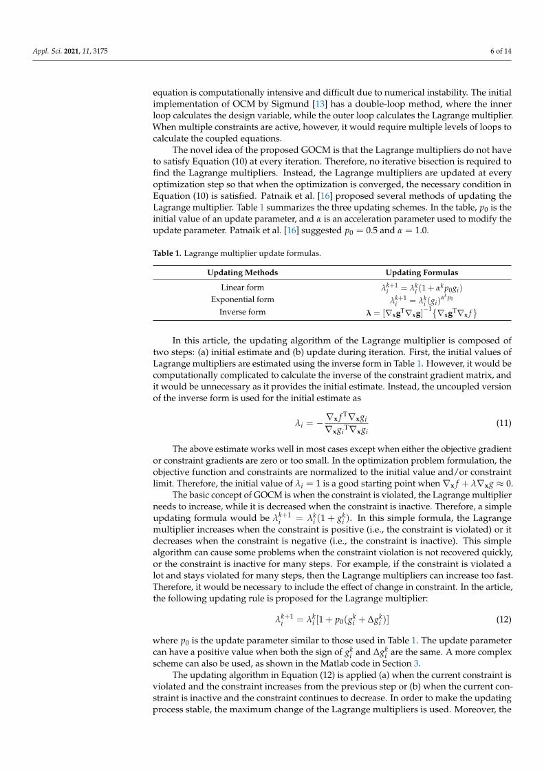
The novel idea of the proposed GOCM is that the Lagrange multipliers do not haveto satisfy Equation (10) at every iteration. Therefore, no iterative bisection is required tofind the Lagrange multipliers. Instead, the Lagrange multipliers are updated at everyoptimization step so that when the optimization is converged, the necessary condition inEquation (10) is satisfied. Patnaik et al. [16] proposed several methods of updating theLagrange multiplier. Table 1 summarizes the three updating schemes. In the table, p0 is theinitial value of an update parameter, and α is an acceleration parameter used to modify theupdate parameter. Patnaik et al. [16] suggested p0 = 0.5 and α = 1.0.
Table 1. Lagrange multiplier update formulas.
Updating Methods Updating Formulas
Linear form λk+1i = λk
i (1 + αk p0gi)
Exponential form λk+1i = λk
i (gi)αk p0
Inverse form λ = [∇xgT∇xg]−1{∇xgT∇x f}
In this article, the updating algorithm of the Lagrange multiplier is composed oftwo steps: (a) initial estimate and (b) update during iteration. First, the initial values ofLagrange multipliers are estimated using the inverse form in Table 1. However, it would becomputationally complicated to calculate the inverse of the constraint gradient matrix, andit would be unnecessary as it provides the initial estimate. Instead, the uncoupled versionof the inverse form is used for the initial estimate as
λi = −∇x f T∇xgi
∇xgiT∇xgi
(11)
The above estimate works well in most cases except when either the objective gradientor constraint gradients are zero or too small. In the optimization problem formulation, theobjective function and constraints are normalized to the initial value and/or constraintlimit. Therefore, the initial value of λi = 1 is a good starting point when ∇x f + λ∇xg ≈ 0.
The basic concept of GOCM is when the constraint is violated, the Lagrange multiplierneeds to increase, while it is decreased when the constraint is inactive. Therefore, a simpleupdating formula would be λk+1
i = λki (1 + gk
i ). In this simple formula, the Lagrangemultiplier increases when the constraint is positive (i.e., the constraint is violated) or itdecreases when the constraint is negative (i.e., the constraint is inactive). This simplealgorithm can cause some problems when the constraint violation is not recovered quickly,or the constraint is inactive for many steps. For example, if the constraint is violated alot and stays violated for many steps, then the Lagrange multipliers can increase too fast.Therefore, it would be necessary to include the effect of change in constraint. In the article,the following updating rule is proposed for the Lagrange multiplier:
λk+1i = λk
i [1 + p0(gki + ∆gk
i )] (12)
where p0 is the update parameter similar to those used in Table 1. The update parametercan have a positive value when both the sign of gk
i and ∆gki are the same. A more complex
scheme can also be used, as shown in the Matlab code in Section 3.The updating algorithm in Equation (12) is applied (a) when the current constraint is
violated and the constraint increases from the previous step or (b) when the current con-straint is inactive and the constraint continues to decrease. In order to make the updatingprocess stable, the maximum change of the Lagrange multipliers is used. Moreover, the
Appl. Sci. 2021, 11, 3175 7 of 14
Lagrange multipliers are limited to change within the lower- and upper-bounds. Since allconstraints are normalized by their bounds, the magnitudes of the Lagrange multipliersare in a similar order of magnitude.
In the theory of Lagrange multiplier, it is well known that it is zero when the constraintis not active, while it is positive when the constraint is active. That means, it is unnecessaryto consider the Lagrange multiplier for inactive constraints and only active constraints areconsidered in the optimization. However, from a practical point of view, it is difficult toturn on and turn off constraints during optimization. Therefore, in the implementation,all constraints and Lagrange multipliers are retained. Then a constraint is inactive, thecorresponding Lagrange multiplier will converge to its lower bound, which reduces itseffect on the optimality criteria.
Once the Lagrange multipliers are updated, the next step of GOCM is to update designvariables. When the optimization problem is composed of the compliance objective andvolume fraction constraint, the scale factor De in Equation (6) is used to update designvariables. This updating algorithm is based on the assumption that that the objectivesensitivity is negative, while the constraint sensitivity is positive. Similar algorithms fordesign variable update were available in Patnaik et al. [16], which are summarized in Table2. All the formulas are based on the scale factor defined as
De = −
NC∑
i=0λi
∂gi∂xe
∂ f∂xe
(13)
Table 2. Design variable update formulas.
Methods Formulas
Linear form xk+1e = xk
e [1 + (De − 1)/(βkq0)]
Exponential form xk+1e = xk
e D1/(βkq0)e
Reciprocal form xk+1e = xk
e /[1− (De − 1)/(βkq0)]
Making De = 1 is equivalent to the stationary condition of Karush–Kuhn–Tuckercondition in Equation (10). The two acceleration parameters in Table 2 are suggested to beq0 = 2.0 and β = 1.0.
In order to consider the general objective and constraints, we need to modify thescale factor in Equation (13). For a given design variable (i.e., element), the scale factor iscalculated on the basis of the sign of sensitivities. The numerator has all terms with negativesensitivities, while the denominator has all terms with positive sensitivities. Accordingly,the scale factor is calculated as
De = −
⟨∂ f∂xe
⟩−+
NC∑
i=1λi
⟨∂gi∂xe
⟩−⟨
∂ f∂xe
⟩++
NC∑
i=1λi
⟨∂gi∂xe
⟩+
(14)
where 〈a〉− = min(0, a) and 〈a〉+ = max(0, a). When De = 1, this formula will also satisfythe stationary condition of the Lagrange function. The only difference is that the originalformulation calculates the scale factor on the basis of the ratio between objective sensitivityand the weighted sum of constraint sensitivities, while the proposed method uses the ratiobetween the positive and negative sensitivities. In the case of compliance objective andvolume fraction constraint, Equations (6), (13), and (14) yield the identical scale factor.
In some special situations, the scale factor needs to be modified. If the numeratorand/or the denominator are zero, the scale factor needs to be limited so that it stays close toone. Moreover, De is scaled such that the design change in each iteration is less than ∆xmax.Once the scale factor is determined, Equation (7) is used to update the design variable.
Appl. Sci. 2021, 11, 3175 8 of 14
3. Numerical Comparisons
In this section, the performance of the proposed GOCM algorithm is compared withthe conventional algorithms, OCM and MMA. The first example is a direct comparisonwith the OCM using Sigmund’s 99-line Matlab code. The other examples are numericalcomparisons with OCM and MMA using Autodesk Nastran.
3.1. Comparison with OCM
Since GOCM is directly related to OCM, it would make sense to compare the perfor-mance between the two. In this section, GOCM is implemented in the 99-line Matlab code.Although GOCM can handle different objectives and multiple constraints, this comparisonis purely based on the compliance objective with volume fraction constraint.
In order to have an objective comparison, we modified the function OC (optimalitycriteria) to GOC for the purpose of GOCM.
In the code, lmid is the Lagrange multiplier with an initial value of 1.0, and gl is thenormalized volume fraction constraint at the previous iteration, with an initial value of 0.0.These values are calculated in the GOC function and returned to the main program. Thealgorithm calculates the scale factor p0 using the normalized constraint, g, and its change,dg. In the main code, the sensitivity is scaled by the initial value of the compliance asdc = dc/f0, where f0 in the initial value of the compliance. In the same way, the sensitivityof the normalized volume fraction constraint becomes 1/nelm, where nelm is the numberof design variables or the number of elements.
Figure 2a shows half of the MBB-beam that was used in Sigmund [13]. The designdomain size is 100 × 50, with the volume fraction constraint of 0.5. Accordingly, thefollowing Matlab command-line is used to launch the topology optimization solver:
top(100,50,0.5,3.0,1.5)
Figure 2b,c show the optimum designs from the OCM and GOCM algorithms, respec-tively, starting from the design domain and boundary conditions given in Figure 2a. Evenif the two optimum designs are slightly different, they are very similar. The optimum objec-tive functions (compliances) were found to be 79.18 (OCM) and 79.05 (GOCM). Therefore,GOCM found slightly smaller compliance than OCM. The number of optimization itera-tions is significantly different in that the OCM converged in 375 iterations, while GOCMin 166 iterations. However, this was the case in the specific example; other examples mayhave a different outcome. The major difference comes from the computational time forsolving the optimality criteria. In order to have a fair comparison, we used Matlab tic andtoc commands before and after calling the OC function. Since OCM takes more iterations,only the time up to 166 iterations were calculated. It turned out that the computational timeof OCM took 10 times longer than that of GOCM. This is expected because OCM needs thebisection method to find the Lagrange multiplier, which normally requires hundreds ofiterations, while the GOCM does not have any iteration.
Appl. Sci. 2021, 11, 3175 9 of 14
Appl. Sci. 2021, 11, x FOR PEER REVIEW 9 of 15
as dc = dc/f0, where f0 in the initial value of the compliance. In the same way, the sensi-tivity of the normalized volume fraction constraint becomes 1/nelm, where nelm is the number of design variables or the number of elements.
Figure 2a shows half of the MBB-beam that was used in Sigmund [13]. The design domain size is ×100 50 , with the volume fraction constraint of 0.5. Accordingly, the fol-lowing Matlab command-line is used to launch the topology optimization solver:
top(100,50,0.5,3.0,1.5)
Figure 2b,c show the optimum designs from the OCM and GOCM algorithms, re-spectively, starting from the design domain and boundary conditions given in Figure 2a. Even if the two optimum designs are slightly different, they are very similar. The opti-mum objective functions (compliances) were found to be 79.18 (OCM) and 79.05 (GOCM). Therefore, GOCM found slightly smaller compliance than OCM. The number of optimi-zation iterations is significantly different in that the OCM converged in 375 iterations, while GOCM in 166 iterations. However, this was the case in the specific example; other examples may have a different outcome. The major difference comes from the computa-tional time for solving the optimality criteria. In order to have a fair comparison, we used Matlab tic and toc commands before and after calling the OC function. Since OCM takes more iterations, only the time up to 166 iterations were calculated. It turned out that the computational time of OCM took 10 times longer than that of GOCM. This is expected because OCM needs the bisection method to find the Lagrange multiplier, which normally requires hundreds of iterations, while the GOCM does not have any iteration.
(a) Design domain
(b) OCM (c) GOCM
Figure 2. Design domain and optimum designs of a cantilevered beam.
Figure 3 shows the optimization histories for OCM and GOCM for the first 80 itera-tions. Both methods showed a similar convergence trend, but the OCM showed smooth variation because it enforced the equality constraint at every iteration. The OCM main-tained =( ) 0g x throughout all iterations, while the GOCM oscillated the positive and negative values until it was stabilized after the 50th iteration. The Lagrange multiplier was converged to 0.6166 (OCM) and 0.6126 (GOCM). This example shows that GOCM and OCM showed a similar optimization trend. However, the GOCM showed oscillation in early design but converged much faster. In addition, the design updating process of GOCM was 10 times faster than that of OCM.
Figure 2. Design domain and optimum designs of a cantilevered beam.
Figure 3 shows the optimization histories for OCM and GOCM for the first 80 iterations.Both methods showed a similar convergence trend, but the OCM showed smooth variationbecause it enforced the equality constraint at every iteration. The OCM maintained g(x) = 0throughout all iterations, while the GOCM oscillated the positive and negative values untilit was stabilized after the 50th iteration. The Lagrange multiplier was converged to 0.6166(OCM) and 0.6126 (GOCM). This example shows that GOCM and OCM showed a similaroptimization trend. However, the GOCM showed oscillation in early design but convergedmuch faster. In addition, the design updating process of GOCM was 10 times faster thanthat of OCM.
Appl. Sci. 2021, 11, x FOR PEER REVIEW 10 of 15
(a) Objective history (b) Constraint history
(c) Lagrange multiplier history
Figure 3. Design optimization histories for optimality criteria method (OCM) and generalized optimality criteria method (GOCM).
3.2. Performance Comparison with OCM and MMA The next example is the gripper-arm model, as shown in Figure 4a. The design do-
main of 127.6 × 43.1 × 10.3 mm3 was modeled by × × ≈135 46 11 68,000 elements. All nodes on the two holes were fixed, and a total of 222.41 N force was uniformly distributed on the upper-right edge as shown in the figure. For material, stainless steel 426 L was used with Young’s modulus of 193 GPa and Poisson’s ratio of 0.25.
In order to have a comparison using all three optimization algorithms, the optimiza-tion problem still uses the minimization of the compliance with volume fraction con-straint, i.e., single objective and single constraint. Therefore, the optimization problem is defined as
=
=
≤
=≤ ≤
T
1
0
min max
Minimize ( ) ( ) { } [ ]{ }
( )subject to 0.09
[ ]{ } { }
eNp
e e e ee
c x
VV
x d k d
x
K D Fx x x
(15)
It is noted that the volume fraction constraint allows only 9% of the material; there-fore, most materials will be removed. The OCM uses the equality constraint, but both MMA and GOCM use the less-than-or-equal-to type constraint. Since the volume fraction constraint is active at the optimum design, both formulations would be identical.
0 20 40 60 80Iteration
50
100
150
200
250
300
350
400
450GOCMOCM
0 20 40 60 80Iteration
0.5
1
1.5
2
2.5
3GOCMOCM
Figure 3. Design optimization histories for optimality criteria method (OCM) and generalized optimality criteriamethod (GOCM).
Appl. Sci. 2021, 11, 3175 10 of 14
3.2. Performance Comparison with OCM and MMA
The next example is the gripper-arm model, as shown in Figure 4a. The design domainof 127.6 × 43.1 × 10.3 mm3 was modeled by 135× 46× 11 ≈ 68, 000 elements. All nodeson the two holes were fixed, and a total of 222.41 N force was uniformly distributed on theupper-right edge as shown in the figure. For material, stainless steel 426 L was used withYoung’s modulus of 193 GPa and Poisson’s ratio of 0.25.
Appl. Sci. 2021, 11, x FOR PEER REVIEW 11 of 15
The optimization problem was solved using Autodesk Nastran 2020 (Autodesk Inc., San Rafael, CA, USA) [19]. At each optimization iteration, using the current design varia-bles, Autodesk Nastran calculated the structural responses, adjoint loads, adjoint re-sponses, and sensitivity of objective and constraints. Then, using this information, the op-timization algorithm calculated new design variables. This iteration was repeated until the convergence criteria were satisfied.
Figure 4 b–d shows the optimum designs using three algorithms. Even if the opti-mum designs were slightly different, the objective and constraint were close to each other, as shown in Table 3. The MMA algorithm tended to make smaller features than other algorithms, but this could be different if the optimization problem started from different initial densities. This was the fundamental limitation of gradient-based optimization, wherein only local optima could be found. An important distinction could be observed in computational times in the last two columns of Table 3. The total time is the time in sec-onds to solve the optimization problem, while the algorithm time is the time that is used in the optimization algorithm. While the MMA took 21% of computational time, the OCM and GOCM took 6% and 0.02%, respectively. The history of the compliance objective dis-played in Figure 5 shows that the OCM showed a smooth variation of the objective, but none of the methods provided a monotonic change of the objective. In this particular ex-ample, both OCM and MMA converged to the optimum design from the feasible domain, while GOCM converged from the infeasible domain. It is also noted that the optimization history of MMA and GOCM showed a saw-tooth type pattern, which was not related to the optimization algorithm. Rather, it was related to the progressive increase of the pen-alty parameter in the SIMP algorithm.
(a) Initial design domain (b) Optimum design using OCM
(c) Optimum design using MMA (d) Optimum design using GOCM
Figure 4. The initial design domain and optimum designs using different methods for the gripper-arm model.
Figure 4. The initial design domain and optimum designs using different methods for the gripper-arm model.
In order to have a comparison using all three optimization algorithms, the optimizationproblem still uses the minimization of the compliance with volume fraction constraint, i.e.,single objective and single constraint. Therefore, the optimization problem is defined as
Minimize c(x) =Ne∑
e=1(xe)
p{de}T[ke]{de}
subject to V(x)V0≤ 0.09
[K]{D} = {F}xmin ≤ x ≤ xmax
(15)
It is noted that the volume fraction constraint allows only 9% of the material; therefore,most materials will be removed. The OCM uses the equality constraint, but both MMA andGOCM use the less-than-or-equal-to type constraint. Since the volume fraction constraintis active at the optimum design, both formulations would be identical.
The optimization problem was solved using Autodesk Nastran 2020 (Autodesk Inc.,San Rafael, CA, USA) [19]. At each optimization iteration, using the current designvariables, Autodesk Nastran calculated the structural responses, adjoint loads, adjointresponses, and sensitivity of objective and constraints. Then, using this information, theoptimization algorithm calculated new design variables. This iteration was repeated untilthe convergence criteria were satisfied.
Appl. Sci. 2021, 11, 3175 11 of 14
Figure 4b–d shows the optimum designs using three algorithms. Even if the optimumdesigns were slightly different, the objective and constraint were close to each other,as shown in Table 3. The MMA algorithm tended to make smaller features than otheralgorithms, but this could be different if the optimization problem started from differentinitial densities. This was the fundamental limitation of gradient-based optimization,wherein only local optima could be found. An important distinction could be observedin computational times in the last two columns of Table 3. The total time is the time inseconds to solve the optimization problem, while the algorithm time is the time that isused in the optimization algorithm. While the MMA took 21% of computational time, theOCM and GOCM took 6% and 0.02%, respectively. The history of the compliance objectivedisplayed in Figure 5 shows that the OCM showed a smooth variation of the objective,but none of the methods provided a monotonic change of the objective. In this particularexample, both OCM and MMA converged to the optimum design from the feasible domain,while GOCM converged from the infeasible domain. It is also noted that the optimizationhistory of MMA and GOCM showed a saw-tooth type pattern, which was not related tothe optimization algorithm. Rather, it was related to the progressive increase of the penaltyparameter in the SIMP algorithm.
Table 3. Comparison of optimum designs using different optimization algorithms.
Algorithm Iteration Compliance Volume Fraction Total Time (s) Algorithm Time (s) Algorithm/Total Time (%)
Figure 5. Optimization history of compliance using three optimization algorithms.
3.3. Performance Comparison for Multiple Constraints In this section, an optimization problem with multiple constraints is used to compare
the performance of different algorithms. As mentioned before, when multiple constraints are present, the OCM cannot be used. Therefore, only MMA and GOCM algorithms can be used. The same gripper-arm model in the previous section was used for the comparison of MMA and GOCM when there were multiple constraints. The design optimization prob-lem is defined as
σ
=
=
≤
≤ ×≤≤≤
=≤ ≤
T
1
07
max
max
max
max
min max
Minimize ( ) ( ) { } [ ]{ }
( ) 0.09subject to
( ) 4.5 100.00010.00010.0001
[ ]{ } { }
eNp
e e e ee
vM
c x
VV
uvw
x d k d
x
K D Fx x x
(16)
The compliance objective and volume fraction constraint are identical to the previous example. In addition, the maximum von Mises stress and the maximum displacement constraints were added. For the maximum von Mises stress, the aggregated P-norm stress
0 20 40 60 80 100Iteration
0
0.02
0.04
0.06
0.08GOCMMAMOCM
Figure 5. Optimization history of compliance using three optimization algorithms.
3.3. Performance Comparison for Multiple Constraints
In this section, an optimization problem with multiple constraints is used to comparethe performance of different algorithms. As mentioned before, when multiple constraintsare present, the OCM cannot be used. Therefore, only MMA and GOCM algorithms can beused. The same gripper-arm model in the previous section was used for the comparison ofMMA and GOCM when there were multiple constraints. The design optimization problemis defined as
Appl. Sci. 2021, 11, 3175 12 of 14
Minimize c(x) =Ne∑
e=1(xe)
p{de}T[ke]{de}
subject to V(x)V0≤ 0.09
(σvM)max ≤ 4.5× 10⁷
umax ≤ 0.0001vmax ≤ 0.0001wmax ≤ 0.0001
[K]{D} = {F}xmin ≤ x ≤ xmax
(16)
The compliance objective and volume fraction constraint are identical to the previousexample. In addition, the maximum von Mises stress and the maximum displacementconstraints were added. For the maximum von Mises stress, the aggregated P-norm stresswas used [20]. For the displacement constraints, a similar P-norm was used to calculate themaximum displacement in each coordinate direction.
Figure 6a,b shows the optimum geometry using GOCM and MMA algorithms, re-spectively. Both methods took 102 iterations to converge, as shown in Table 4. In thisoptimization problem, GOCM found an optimum design whose compliance was about 8%less than that of MMA. Among five inequality constraints, the volume fraction, maximumy-displacement, and maximum von Mises stress were active at the optimum design. TheMMA algorithm took 32% of the total time. Considering that the remaining 68% of the timewas used for calculating structural response, adjoint load, adjoint response, and adjointsensitivity, the optimization algorithm took a significant portion of the time. Compared tothe MMA, the GOCM algorithm took a fraction of a second, which provides a significantadvantage over MMA. It is interesting to note that the MMA algorithm became compu-tationally expensive when constraints became active. As shown in Figure 7, initially theMMA algorithm took about 1.5 s for each iteration, but after the 40th iteration, it tookabout 15 s for each iteration, where constraints became active. This is because the MMAsubproblem can be expensive when multiple constraints are active.
Appl. Sci. 2021, 11, x FOR PEER REVIEW 13 of 15
was used [20]. For the displacement constraints, a similar P-norm was used to calculate the maximum displacement in each coordinate direction.
Figure 6a,b shows the optimum geometry using GOCM and MMA algorithms, re-spectively. Both methods took 102 iterations to converge, as shown in Table 4. In this op-timization problem, GOCM found an optimum design whose compliance was about 8% less than that of MMA. Among five inequality constraints, the volume fraction, maximum y-displacement, and maximum von Mises stress were active at the optimum design. The MMA algorithm took 32% of the total time. Considering that the remaining 68% of the time was used for calculating structural response, adjoint load, adjoint response, and ad-joint sensitivity, the optimization algorithm took a significant portion of the time. Com-pared to the MMA, the GOCM algorithm took a fraction of a second, which provides a significant advantage over MMA. It is interesting to note that the MMA algorithm became computationally expensive when constraints became active. As shown in Figure 7, ini-tially the MMA algorithm took about 1.5 s for each iteration, but after the 40th iteration, it took about 15 s for each iteration, where constraints became active. This is because the MMA subproblem can be expensive when multiple constraints are active.
(a) GOCM (b) MMA
Figure 6. Optimum design of the gripper-arm model with multiple constraints.
Table 4. Comparison of optimum designs with multiple constraints.
Total time (s) 2541 1580Algorithm time (s) 820 0.15
Algorithm/total time (%) 32.3 0.01
Appl. Sci. 2021, 11, 3175 13 of 14Appl. Sci. 2021, 11, x FOR PEER REVIEW 14 of 15
Figure 7. Accumulated optimization algorithm time for the method of moving asymptotes (MMA).
4. Conclusions In this article, a new topology optimization algorithm, the generalized optimality cri-
teria method (GOCM), was proposed. It is based on the conventional optimality criteria method (OCM), wherein both Lagrange multiplier and design variables are updated. The main difference is that the proposed method can have multiple inequality constraints, while the OCM can only support a single constraint (e.g., volume fraction). The Lagrange multipliers were updated on the basis of the constraint violation and constraint change. Then, the design variables were updated toward the direction to satisfy the optimality criteria. Therefore, constraints may not have been satisfied during the optimization itera-tion, but they were satisfied upon convergence. Numerical examples showed that the pro-posed method was faster than the OCM and the method of moving asymptotes (MMA). In the case of a MATLAB-based 2D model with 5000 design variables, GOCM was 10 times faster than OCM. In the case of the gripper-arm model (68,000 elements), GOCM was more than 1000 times faster than MMA and 330 times faster than OCM. When there were multiple constraints, the optimization time became comparable with that of finite element simulation times. In the case of MMA, the optimization algorithm time was about 35% of the total time, while the optimization time of GOCM was negligible. Therefore, the pro-posed method was versatile to handle multiple constraints, while computationally effi-cient.
For future research, it would be beneficial to handle active and inactive constraints separately. The current implementation updated the Lagrange multipliers for both active and inactive constraints, but it would be necessary to remove the effect of inactive con-straints completely from optimality criteria. In GOCM, it is possible that constraints are consistently violated during iterations and only the final converged design satisfies the constraints. In order to make un-converged designs useful, it would be beneficial that de-signs are updated in the feasible region.
Author Contributions: Conceptualization, N.H.K.; methodology, N.H.K. and T.D.; software, D.W.; validation, N.H.K.; formal analysis, T.D.; investigation, J.D.; resources, D.W.; data curation, T.D.; writing—original draft preparation, N.H.K.; writing—review and editing, N.H.K.; visualization, J.D.; supervision, N.H.K. All authors have read and agreed to the published version of the manu-script.
Funding: This research received no external funding.
0 20 40 60 80 100Iteration
0
200
400
600
800
1000
Figure 7. Accumulated optimization algorithm time for the method of moving asymptotes (MMA).
4. Conclusions
In this article, a new topology optimization algorithm, the generalized optimalitycriteria method (GOCM), was proposed. It is based on the conventional optimality criteriamethod (OCM), wherein both Lagrange multiplier and design variables are updated. Themain difference is that the proposed method can have multiple inequality constraints,while the OCM can only support a single constraint (e.g., volume fraction). The Lagrangemultipliers were updated on the basis of the constraint violation and constraint change.Then, the design variables were updated toward the direction to satisfy the optimality cri-teria. Therefore, constraints may not have been satisfied during the optimization iteration,but they were satisfied upon convergence. Numerical examples showed that the proposedmethod was faster than the OCM and the method of moving asymptotes (MMA). In thecase of a MATLAB-based 2D model with 5000 design variables, GOCM was 10 times fasterthan OCM. In the case of the gripper-arm model (68,000 elements), GOCM was more than1000 times faster than MMA and 330 times faster than OCM. When there were multipleconstraints, the optimization time became comparable with that of finite element simu-lation times. In the case of MMA, the optimization algorithm time was about 35% of thetotal time, while the optimization time of GOCM was negligible. Therefore, the proposedmethod was versatile to handle multiple constraints, while computationally efficient.
For future research, it would be beneficial to handle active and inactive constraintsseparately. The current implementation updated the Lagrange multipliers for both activeand inactive constraints, but it would be necessary to remove the effect of inactive con-straints completely from optimality criteria. In GOCM, it is possible that constraints areconsistently violated during iterations and only the final converged design satisfies theconstraints. In order to make un-converged designs useful, it would be beneficial thatdesigns are updated in the feasible region.
Author Contributions: Conceptualization, N.H.K.; methodology, N.H.K. and T.D.; software, D.W.;validation, N.H.K.; formal analysis, T.D.; investigation, J.D.; resources, D.W.; data curation, T.D.;writing—original draft preparation, N.H.K.; writing—review and editing, N.H.K.; visualization, J.D.;supervision, N.H.K. All authors have read and agreed to the published version of the manuscript.
Funding: This research received no external funding.
Institutional Review Board Statement: Not applicable.
Informed Consent Statement: Not applicable.
Data Availability Statement: Autodesk Nastran input files are available.
Conflicts of Interest: The authors declare no conflict of interest.
Appl. Sci. 2021, 11, 3175 14 of 14
References1. Bendsøe, M.P. Optimization of Structural Topology, Shape and Material; Springer: Berlin/Heidelberg, Germany, 1995.2. Svanberg, K. The method of moving asymptotes—A new method for structural optimization. Int. J. Numer. Methods Eng. 1987, 24,
359–373. [CrossRef]3. Dunning, P.D.; Kim, H.A. Introducing the sequential linear programming level-set method for topology optimization. Struct.
Multidiscip. Optim. 2015, 51, 631–643. [CrossRef]4. Siva, L.; Mahesh, N.; Sateesh, N. Topology optimization using solid isotropic material with penalization technique for additive
manufacturing. Mater. Today Proc. 2017, 4, 1414–1422. [CrossRef]5. Wang, S.; Tai, K. Structural topology design optimization using Genetic Algorithms with a bit-array representation. Comput.
Methods Appl. Mech. Eng. 2005, 194, 3749–3770. [CrossRef]6. Lynn, N.; Ali, M.; Suganthan, P. Population topologies for particle swarm optimization and differential evolution. Swarm Evol.
Comput. 2018, 39, 24–35. [CrossRef]7. Bureerat, S.; Limtragool, J. Structural topology optimisation using simulated annealing with multiresolution design variables.
Finite Elements Anal. Des. 2008, 44, 738–747. [CrossRef]8. Gao, F.; Han, L. Implementing the Nelder-Mead simplex algorithm with adaptive parameters. Comput. Optim. Appl. 2010, 51,
259–277. [CrossRef]9. Haftka, R.T. Requirements for papers focusing on new or improved global optimization algorithms (Editorial). Struct. Multidiscip.
Optim. 2016, 54, 1. [CrossRef]10. Zhou, Y.; Saitou, K. Gradient-based multi-component topology optimization for stamped sheet metal assemblies (MTO-S). Struct.
Multidiscip. Optim. 2018, 58, 83–94. [CrossRef]11. Allaire, G. A review of adjoint methods for sensitivity analysis, uncertainty quantification and optimization in numerical codes.
Ingénieurs l’Automobile SIA 2015, 836, 33–36.12. Roosta, F.; Liu, Y.; Xu, P.; Mahoney, M. Newton-MR: Newton’s Method Without Smoothness or Convexity. arXiv 2018,
arXiv:1810.00303.13. Sigmund, O. A 99 line topology optimization code written Matlab. Struct. Multidiscip. Optim. 2016, 21, 120–127. [CrossRef]14. Jiang, T.; Papalambros, P.Y. A first order method of moving asymptotes for structural optimization. Trans. Build Environ. 1995, 13,
75–83.15. Arora, J.S. Introduction to Optimal Design; McGraw-Hill: New York, NY, USA, 1988.16. Patnaik, S.N.; Guptill, J.D.; Berke, L. Merits and Limitations of Optimality Criteria Method for Structural Optimization; NASA Technical
Paper 3373; National Aeronautics and Space Administration: Cleveland, OH, USA, 1993.17. Berke, L.; Khot, N.S. Structural optimization using optimality criteria. Comput. Aided Optim. Des. Struct. Mech. Syst. 1987, 27,
271–311.18. Sands, T. Optimization Provenance of Whiplash Compensation for Flexible Space Robotics. Aerospace 2019, 6, 93. [CrossRef]19. Weinberg, D.J. Autodesk Inventor Nastran 2020 User’s Manual; Autodesk Inc.: San Rafael, CA, USA, 2019.20. Park, Y.K. Extensions of Optimal Layout Design Using the Homogenization Method. Ph.D. Thesis, University of Michigan,