Generalized Optimization: A First Step Towards Category Theoretic Learning Theory Dan Shiebler [email protected]University of Oxford September 22, 2021 Abstract The Cartesian reverse derivative is a categorical generalization of reverse- mode automatic differentiation. We use this operator to generalize several optimization algorithms, including a straightforward generalization of gra- dient descent and a novel generalization of Newton’s method. We then explore which properties of these algorithms are preserved in this general- ized setting. First, we show that the transformation invariances of these algorithms are preserved: while generalized Newton’s method is invari- ant to all invertible linear transformations, generalized gradient descent is invariant only to orthogonal linear transformations. Next, we show that we can express the change in loss of generalized gradient descent with an inner product-like expression, thereby generalizing the non-increasing and convergence properties of the gradient descent optimization flow. Fi- nally, we include several numerical experiments to illustrate the ideas in the paper and demonstrate how we can use them to optimize polynomial functions over an ordered ring. 1 Background Given a convex differentiable function l : R n → R, there are many algorithms that we can use to minimize it. For example, if we pick a step size α and a starting point x 0 ∈ R n we can apply the gradient descent algorithm in which we repeatedly iterate x t+1 = x t - α *∇l(x t ). For small enough α this strategy is guaranteed to get close to the x that minimizes l (Boyd and Vandenberghe, 2004). Algorithms like gradient descent are often useful even when l is non-convex. For example, under relatively mild conditions we can show that taking small enough gradient descent steps will never increase the value of any differentiable l : R n → R (Boyd and Vandenberghe, 2004). The modern field of deep learning consists largely of applying gradient descent and other algorithms that can be 1 arXiv:2109.10262v1 [math.OC] 20 Sep 2021
The Cartesian reverse derivative is a categorical generalization of reverse-mode automatic differentiation. We use this operator to generalize severaloptimization algorithms, including a straightforward generalization of gra-dient descent and a novel generalization of Newton’s method. We thenexplore which properties of these algorithms are preserved in this general-ized setting. First, we show that the transformation invariances of thesealgorithms are preserved: while generalized Newton’s method is invari-ant to all invertible linear transformations, generalized gradient descent isinvariant only to orthogonal linear transformations. Next, we show thatwe can express the change in loss of generalized gradient descent withan inner product-like expression, thereby generalizing the non-increasingand convergence properties of the gradient descent optimization flow. Fi-nally, we include several numerical experiments to illustrate the ideas inthe paper and demonstrate how we can use them to optimize polynomialfunctions over an ordered ring.
1 Background
Given a convex differentiable function l : Rn → R, there are many algorithmsthat we can use to minimize it. For example, if we pick a step size α and astarting point x0 ∈ Rn we can apply the gradient descent algorithm in whichwe repeatedly iterate xt+1 = xt − α ∗ ∇l(xt). For small enough α this strategyis guaranteed to get close to the x that minimizes l (Boyd and Vandenberghe,2004).
Algorithms like gradient descent are often useful even when l is non-convex.For example, under relatively mild conditions we can show that taking smallenough gradient descent steps will never increase the value of any differentiablel : Rn → R (Boyd and Vandenberghe, 2004). The modern field of deep learningconsists largely of applying gradient descent and other algorithms that can be
1
arX
iv:2
109.
1026
2v1
[m
ath.
OC
] 2
0 Se
p 20
21
efficiently computed with reverse-mode automatic differentiation to optimizenon-convex functions (LeCun et al., 2015).
While gradient descent is particularly popular, it is not the only gradient-based optimization algorithm that is widely used in practice. Both the momen-tum and Adagrad algorithms use placeholder variables that store informationfrom previous gradient updates to improve stability. Newton’s method, whichrescales the gradient with the inverse Hessian matrix, is popular for many appli-cations but less commonly used in deep learning due to the difficulty of efficientlyimplementing it with reverse-mode automatic differentiation. Each of these al-gorithms have different invariance properties that affect their stability underdataset transformations: for example, Newton’s method enjoys an invariance tolinear rescaling that gradient descent lacks.
Given the utility of these algorithms it is natural to explore when they canbe generalized beyond differentiable functions. For example, if we replace thegradient in gradient descent with a representative of the subgradient, a simplegeneralization of the gradient for non-differentiable functions l : Rn → R, theconvergence and stability properties of gradient descent are preserved (Boydand Vandenberghe, 2004). Going one step further, some authors have begunto explore generalizations of differentiation beyond Euclidean spaces. Cockettet al. (2019) introduce Cartesian reverse derivative categories in which we candefine an operator that shares certain properties with reverse-mode automaticdifferentiation (RD.1 to RD.7 in Definition 13 of Cockett et al. (2019)). Reversederivative categories are remarkably general: the category of Euclidean spacesand differentiable functions between them is of course a reverse derivative cat-egory, as are the categories of polynomials over semirings and the category ofBoolean circuits (Wilson and Zanasi, 2021).
In this paper we explore whether the convergence and invariance propertiesof optimization algorithms built on top of the gradient and Hessian generalize tooptimization algorithms built on top of Cockett et al. (2019)’s Cartesian reversederivative. Our contributions are as follows:
• We use Cockett et al. (2019)’s Cartesian reverse derivative to define gen-eralized analogs of several optimization algorithms, including a novel gen-eralization of Newton’s method.
• We derive novel results on the transformation invariances of these gener-alized algorithms.
• We define the notion of an optimization domain over which we can applythese generalized algorithms and study their convergence properties.
• We characterize the properties that an optimization domain must satisfy inorder to support generalized gradient-based optimization and we providenovel results that the optimization domain of polynomials over orderedrings satisfies these properties.
• We include several numerical experiments to illustrate the ideas in the pa-per and demonstrate how we can use them to optimize polynomial func-
2
tions over an ordered ring. The code to run these experiments is on Githubat tinyurl.com/ku3pjz56.
2 Standard Optimization
As we described in Section 1, gradient descent optimizes an objective functionl : Rn → R by starting at a point x0 ∈ Rn and progressing the discrete dynamicalsystem xt+1 = xt−α∗∇l(xt). Rewriting this as xt+α = xt−α∗∇l(xt) and takingthe limα→0 of this system yields the differential equation ∂x
∂t (t) = −∇l(x(t)),which we can think of as the continuous limit of gradient descent. More generallywe have:
Definition 2.1. An optimizer for l : Rn → R with dimension k is a contin-uous function d : Rkn → Rkn.
Intuitively, an optimizer defines both a continuous and a discrete dynamicalsystem
Note that the discrete dynamical system is the Euler’s method discretization ofthe continuous system. We can think of an optimizer with dimension k > 1 asusing information beyond the previous value xt to determine xt+1.
In practice we usually work with optimizers that define dynamical systemsin which l(x(t)) and l(xt) get closer to the minimum value of l as t increases.Given l : Rn → R we can construct the following examples:
• The gradient descent optimizer for l : Rn → R is d(x) = −∇l(x). Thisoptimizer has dimension 1.
• The Newton’s method optimizer for l : Rn → R is d(x) = −∇2(l(x))−1∇l(x).This optimizer has dimension 1 and uses the inverse Hessian matrix to in-crease the stability of each update.
• The momentum optimizer for l : Rn → R is d(x, y) = (y,−y −∇l(x)).This optimizer has dimension 2 and uses a placeholder variable to trackthe value of the previous update steps and simulate the momentum of aball rolling down a hill.
• The Adagrad optimizer for l : Rn → R is d(x, y) = (−∇l(x)/√y,∇l(x)2).
This optimizer has dimension 2 and uses a placeholder variable to reweightupdates based on the magnitude of previous updates (Duchi et al., 2011).
3
2.1 Optimization Schemes
Definition 2.2. An optimization scheme u : (Rn → R)→ (Rkn → Rkn) is afamily of functions (indexed by n) that maps objectives l : Rn → R to optimizersd : Rkn → Rkn.
For example, the gradient descent optimization scheme is u(l)(x) = −∇l(x)and the momentum optimization scheme is u(l)(x, y) = (y,−y −∇l(x)).
In some situations we may be able to improve the convergence rate of the dy-namical systems defined by optimization schemes by precomposing an invertiblefunction f : Rm → Rn. That is, rather than optimize the function l : Rn → Rwe optimize l ◦ f : Rm → R. However, for many optimization schemes thereare classes of transformations to which they are invariant: applying any suchtransformation to the data cannot change the trajectory.
Definition 2.3. Suppose f : Rm → Rn is an invertible transformation andwrite fk for the map (f × f × · · · ) : Rkm → Rkn. The optimization scheme u isinvariant to f if u(l ◦ f) = f−1k ◦ u(l) ◦ fk.
Proposition 1. Recall that an invertible linear transformation is a functionf(x) = Ax where the matrix A has an inverse A−1 and an orthogonal lineartransformation is an invertible linear transformation where A−1 = AT . New-ton’s method is invariant to all invertible linear transformations, whereas bothgradient descent and momentum are invariant to orthogonal linear transforma-tions. (Proof in Appendix A.1).
Note that Adagrad is not invariant to orthogonal linear transformations dueto the fact that it tracks a nonlinear function of past gradients (sum of squares).In order to interpret these invariance properties it is helpful to consider how theyaffect the discrete dynamical system defined by an optimization scheme.
Proposition 2. Given an objective function l : Rn → R and an optimizationscheme u : (Rn → R) → (Rkn → Rkn) that is invariant to the invertible linearfunction f : Rm → Rn, the discrete system defined by the optimizer u(l ◦ f):
yt+1 = yt + αu(l ◦ f)(yt)
cannot converge faster than the discrete system defined by the optimizer u(l):
xt+1 = xt + αu(l)(xt)
(Proof in Appendix A.2).
Propositions 1 and 2 together give some insight into why Newton’s methodcan perform so much better than gradient descent for applications where bothmethods are computationally feasible (Boyd and Vandenberghe, 2004). Whereasgradient descent can be led astray by bad data scaling, Newton’s method stepsare always scaled optimally and therefore cannot be improved by data rescaling.
It is important to note that Proposition 2 only applies to linear transfor-mation functions f . Since Euler’s method is itself a linear method, it does notnecessarily preserve non-linear invariance properties.
4
3 Generalized Optimization
In this section we assume readers have a basic familiarity with Category The-ory. We recommend that readers who would like a detailed introduction to thefield check out “Basic Category Theory” (Leinster, 2016) or “Seven Sketches inCompositionality” (Fong and Spivak, 2019).
3.1 Cartesian and Reverse Derivative Categories
We begin by recalling some basic terminology and notation. A category isa collection of objects and morphisms between them. Morphisms are closedunder an associative composition operation, and each object is equipped withan identity morphism. An example category is the collection of sets (objects)and functions (morphisms) between them. We call the set of morphisms betweenthe objects A and B in the category C the hom-set C[A,B].
A category is Cartesian when there exists a product operation × that allowsus to combine objects, a pairing operation 〈−,−〉 that allows us to combinemorphisms, projection maps π0 : A × B → A, π1 : A × B → B and a terminalobject ∗ such that every object A is equipped with a unique map !A : A→ ∗ fromA to the terminal object ∗. Given an object A or morphism f in a Cartesiancategory, in this work we write Ak and fk to respectively denote A and ftensored with themselves k times.
Now recall the following definition from Richard F Blute (2009); Cockettet al. (2019):
Definition 3.1. A Cartesian left additive category is a Cartesian categoryC in which the hom-set of each pair of objects B,C is a commutative monoid,with addition operation + and zero maps (additive identities) 0BC : B → C,such that:
• For any morphism h : A→ B and f, g : B → C we have:
(f + g) ◦ h = (f ◦ h) + (g ◦ h) : A→ C 0BC ◦ h = 0AC : A→ C
• For any projection map πi : C → D and f, g : B → C we have:
πi ◦ (f + g) = (πi ◦ f) + (πi ◦ g) : B → D πi ◦ 0BC = 0BD : B → D
We write 0A for the additive identity of the hom-set C[∗, A].
Intuitively, in a Cartesian left additive category we can add morphisms ina way that is compatible with postcomposition and the Cartesian structure.Certain Cartesian left additive categories are equipped with additional structurethat behaves similarly to derivatives:
Definition 3.2. A Cartesian reverse derivative category is a Cartesianleft-additive category C equipped with a Cartesian reverse derivative com-binator R that assigns to each morphism f : A → B in C a morphismR[f ] : A × B → A in C such that R satisfies the following equations (Defi-nition 13 of (Cockett et al., 2019)):
where ι0 : A → A × B and ι1 : B → A × B are the Cartesian injection maps(Cockett et al., 2019).
The conditions RD.1 to RD.7 mirror the properties of the derivative op-eration. For example, R must commute with addition (RD.1) and composeaccording to a chain rule (RD.5).
Definition 3.3. A Cartesian differential category C is a Cartesian left-additive category equipped with a Cartesian derivative combinator D thatassigns to each morphism f : A → B in C a morphism D[f ] : A × A → B inC such that D satisfies the following equations (Definition 4 in Cockett et al.(2019), adapted from Definition 2.1.1 in (Richard F Blute, 2009)):
By Theorem 16 in (Cockett et al., 2019), every Cartesian reverse derivativecategory C is also a Cartesian differential category where for any morphismf : A→ B in C:
Going forward, when we refer to the Cartesian derivative combinator D of aCartesian reverse derivative category this is the construction that we are refer-ring to.
6
The canonical example of a Cartesian reverse derivative category that wewill consider is the category Euc of Euclidean spaces and infinitely differen-tiable maps between them. The terminal object ∗ in Euc is R0, the Cartesianreverse derivative of the map f : Ra → Rb is R[f ](x, x′) = Jf (x)Tx′, and theCartesian derivative of f is D[f ](x, x′) = Jf (x)x′ where Jf (x) is the Jacobianof f evaluated at x ∈ Ra. Recall that the Jacobian of f : Ra → Rb is a b × amatrix whose i, jth element is ∂fi
∂xj.
As another example, given a commutative ring r we can form the categoryPolyr in which objects are natural numbers and the morphisms from n tom are tuples of m polynomials with n variables and coefficients in r. Thatis, a morphism P : n → m is a map P (x) = (p1(x), · · · , pm(x)) where x =(x1, · · · , xn) and pi is a polynomial. Polyr is a Cartesian reverse derivativecategory in which the terminal object ∗ is 0 and the reverse derivative of P (x) =(p1(x), · · · , pm(x)) is:
R[P ](x, x′) =
(m∑i=1
∂pi∂x1
(x)x′i, · · · ,m∑i=1
∂pi∂xn
(x)x′i
)
where ∂pi∂xj
(x) is the formal derivative of pi in xj , evaluated at x (Cockett et al.,
2019).The linear maps in a Cartesian reverse derivative category C are those for
which D[f ] = f ◦ π1. The linear maps of C form a subcategory of C equippedwith a stationary on objects involution ( )† : Cop → C such that for any linearmap f we have R[f ] = f† ◦ π1 (Cockett et al., 2019).
The linear maps in Euc are exactly the linear maps in the traditional sense,and given a linear map f : Ra → Rb in Euc where f(x) = Mx we havef† : Rb → Ra where f†(x) = MTx. That is, † is a generalization of thetranspose. Similarly, the linear maps in Polyr are those that can be expressedas P (x) = (p1(x), · · · , pm(x)) where pi(x) =
∑ni=1 rixi for ri ∈ r (Cockett et al.,
2019).
3.2 Optimization Domain
Definition 3.4. An optimization domain is a tuple (Base, X) such that eachmorphism f : A→ B in the Cartesian reverse derivative category Base has anadditive inverse −f and each homset C[∗, A] out of the terminal object ∗ isfurther equipped with a multiplication operation fg and a multiplicative identitymap 1A : ∗ → A to form a commutative ring with the left additive structure +.X is an object in Base such that the homset f ∈ C[∗, X] is further equippedwith a total order f ≤ g to form an ordered commutative ring.
Given an optimization domain (Base, X) the object X represents the spaceof objective values to optimize and we refer to morphisms into X as objectives.We abbreviate the map 1B◦!A : A→ B as 1AB , where !A : A→ ∗ is the uniquemap into the terminal object ∗. For example, the objectives in the standarddomain (Euc,R) are functions l : Rn → R. If r is an ordered commutative ring
7
then we can form the r-polynomial domain (Polyr, 1) in which objectives arer-polynomials lP : n→ 1.
Definition 3.5. We say that an objective l : A → X is bounded below in(Base, X) if there exists some x : ∗ → X such that for any a : ∗ → A we havex ≤ l ◦ a.
In both the standard and r-polynomial domains an objective is boundedbelow if its image has an infimum.
3.2.1 Generalized Gradient and Generalized n-Derivative
Definition 3.6. The generalized gradient of the objective l : A → X in(Base, X) is R[l]1 : A→ A where:
R[l]1 = R[l] ◦ 〈idA, 1AX〉
In the standard domain the generalized gradient of l : Rn → R is justthe gradient R[l]1(x) = ∇l(x) and in the r-polynomial domain the generalized
gradient of lP : n → 1 is R[lP ]1(x) =(∂lP∂x1
(x), · · · , ∂lP∂xn(x))
where ∂lP∂xi
is the
formal derivative of the polynomial lP in xi.
Definition 3.7. The generalized n-derivative of the morphism f : X → Ain (Base, X) is Dn[f ] : X → A where:
In the standard domain the generalized n-derivative of f : R → R is then-derivative f (n) = ∂nf
∂xn and in the r-polynomial domain the generalized n-
derivative of lP : 1→ 1 is the formal n-derivative ∂nlP∂xn .
The derivative over the reals has a natural interpretation as a rate of change.We can generalize this as follows:
Definition 3.8. We say that a morphism f : X → X in Base is n-smooth in(Base, X) if whenever Dk[f ] ◦ t ≥ 0X : ∗ → X for all t1 ≤ t ≤ t2 : ∗ → X andk ≤ n we have that f ◦ t1 ≤ f ◦ t2 : ∗ → X.
Intuitively, f is n-smooth if it cannot decrease on any interval over which itsgeneralized derivatives of order n and below are non-negative. Some examplesinclude:
• Any map f : R → R is 1-smooth in the standard domain by the meanvalue theorem.
• When r is a dense subring of a real-closed field then any polynomial lP :1→ 1 is 1-smooth in the r-polynomial domain (Nombre, 2021).
8
• For any r, the polynomial lP =∑nk=0 ckt
k : 1→ 1 of degree n is n-smoothin the r-polynomial domain since for any t1 we can use the binomial the-orem to write:
lP (t) =
n∑k=0
cktk =
n∑k=0
ck(t1 + (t− t1))k = lP (t1) +
n∑k=1
c′k(t− t1)k
where c′k is a constant such that (c′k)(k!) = Dk[lP ](t1). Note that c′kmust exist by the definition of the formal derivative of lP , and must benon-negative if Dk[lP ](t1) is non-negative.
3.3 Optimization Functors
In this section we generalize optimization schemes (Section 2.1) to arbitrary op-timization domains. This will enable us to characterize the invariance propertiesof our generalized optimization schemes in terms of the categories out of whichthey are functorial. Given an optimization domain (Base, X) we can define thefollowing categories:
Definition 3.9. The objects in the category Objective over the optimizationdomain (Base, X) are objectives l : A → X such that there exists an inversefunction R[l]−11 : A→ A where R[l]−11 ◦R[l]1 = R[l]1◦R[l]−11 = idA : A→ A, andthe morphisms between l : A → X and l′ : B → X are morphisms f : A → Bwhere l′ ◦ f = l.
Note that Objective is a subcategory of the slice category Base/X.In the standard domain the objects in Objective are objectives l : Rn → R
such that the function ∇l : Rn → Rn is invertible. In the r-polynomial domain,the objects in Objective are r-polynomials lP : n → 1 such that the function〈 ∂lP∂x1
, · · · , ∂lP∂xn〉 : n→ n is invertible.
Definition 3.10. A generalized optimizer over the optimization domain(Base, X) with state space A ∈ Base and dimension k ∈ N is an endo-morphism d : Ak → Ak in Base. The objects in the category Optimizer over(Base, X) are generalized optimizers, and the morphisms between the general-ized optimizers d : Ak → Ak and d′ : Bk → Bk are Base-morphisms f : A→ Bsuch that fk ◦ d = d′ ◦ fk : Ak → Bk. Note that morphisms only exist betweengeneralized optimizers with the same dimension. The composition of morphismsin Optimizer is the same as in Base.
Recall that Ak and fk are respectively A and f tensored with themselves ktimes. In the standard domain a generalized optimizer with dimension k is atuple (Rn, d) where d : Rkn → Rkn is an optimizer (Definition 2.1).
Definition 3.11. Given a subcategory D of Objective, an optimizationfunctor over D is a functor D → Optimizer that maps the objective l :A→ X to a generalized optimizer over (Base, X) with state space A.
9
Optimization functors are generalizations of optimization schemes (Defini-tion 2.2) that map objectives to generalized optimizers. Explicitly, an optimiza-tion scheme u that maps l : Rn → R to u(l) : Rkn → Rkn defines an optimizationfunctor in the standard domain.
The invariance properties of optimization functors are represented by thesubcategory D ⊆ Objective out of which they are functorial. Concretely,consider the following categories:
• ObjectiveI : The subcategory of Objective in which morphisms are lim-ited to invertible linear morphisms l in Base.
• Objective⊥: The subcategory of ObjectiveI in which the inverse of l isl†.
In both the standard domain and r-polynomial domain, the morphisms inObjectiveI are linear maps defined by an invertible matrix and the morphismsin Objective⊥ are linear maps defined by an orthogonal matrix (matrix inverseis equal to matrix transpose). We will now generalize Proposition 1 by defininggeneralized gradient descent and momentum functors that are functorial out ofObjective⊥ and a generalized Newton’s method functor that is functorial outof ObjectiveI .
Definition 3.12. Generalized gradient descent sends the objective l : A→X to the generalized optimizer −R[l]1 : A→ A with dimension 1.
Definition 3.13. Generalized momentum sends the objective l : A→ X tothe generalized optimizer 〈π1,−π1 − (R[l]1 ◦ π0)〉 : A2 → A2 with dimension 2.
Generalized momentum and generalized gradient descent have a very sim-ilar structure, with the major difference between the two being that general-ized momentum uses a placeholder variable and generalized gradient descentdoes not. In the standard domain we have that −R[l]1(x) = −∇l(x) and(〈π1,−π1−(R[l]1 ◦π0)〉)(x, y) = (y,−y−∇l(x)), so generalized gradient descentand generalized momentum are equivalent to the gradient descent and momen-tum optimization schemes that we defined in Section 2.1. Similarly, in ther-polynomial domain generalized gradient descent maps lP : n→ 1 to −R[lP ]1 :n→ n and generalized momentum maps lP to 〈π1,−π1−(R[lP ]1◦π0)〉 : n2 → n2
where:
〈π1,−π1 − (R[lP ]1 ◦ π0)〉(x, x′) =
(x′,−x′ −
(∂lP∂x1
(x), · · · , ∂lP∂xn
(x)
))Since Newton’s method involves the computation of an inverse Hessian it isnot immediately obvious how we can express it in terms of Cartesian reversederivatives. However, by the inverse function theorem we can rewrite the inverseHessian as the Jacobian of the inverse gradient function, which makes this easier.That is:
(∇2l)(x)−1 = J∇l(x)−1 = J(∇l)−1(∇l(x)) (1)
10
where J∇l(x) = (∇2l)(x) is the Hessian of l at x, J(∇l)−1(∇l(x)) is the Jacobianof the inverse gradient function evaluated at ∇l(x), and the second equalityholds by the inverse function theorem. We can therefore generalize the Newton’smethod term −∇2(l)−1∇l as −R[R[l]−11 ]◦ 〈R[l]1, R[l]1〉 : X → X and generalizeNewton’s method as follows:
Definition 3.14. Generalized Newton’s method sends the objective l : A→X to the generalized optimizer −R[R[l]−11 ]◦〈R[l]1, R[l]1〉 : A→ A with dimension1.
Equation 1 implies that generalized Newton’s method in the standard do-main is equivalent to the Newton’s method optimization scheme that we definedin Section 2.1. In the r-polynomial domain generalized Newton’s Method mapsthe polynomial lP : n→ 1 to −R[R[lP ]−11 ] ◦ 〈R[lP ]1, R[lP ]1〉 : n→ n where:
−R[R[lP ]−11 ] ◦ 〈R[lP ]1, R[lP ]1〉(x) =
−
∂(R[lP ]−1
1 )1∂x1
(R[lP ]1(x)) . . .∂(R[lP ]−1
1 )1∂xn
(R[lP ]1(x))...
. . .∂(R[lP ]−1
1 )n∂x1
(R[lP ]1(x))∂(R[lP ]−1
1 )n∂xn
(R[lP ]1(x))
T (
∂lP∂x1
(x), · · · , ∂lP∂xn
(x)
)
Note that (R[lP ]−11 )i is the ith projection of the inverse of the reverse derivativemap. We now generalize Proposition 1:
Proposition 3. Generalized Newton’s method is a functor from ObjectiveI toOptimizer, whereas both generalized gradient descent and generalized momen-tum are functors from Objective⊥ to Optimizer. (Proof in Appendix A.3)
Proposition 3 implies that the invariance properties of our optimization func-tors mirror the invariance properties of their optimization scheme counterparts.Not only does Proposition 3 directly imply Proposition 1, but it also impliesthat the invariance properties that gradient descent, momentum, and Newton’smethod enjoy are not dependent on the underlying category over which theyare defined.
3.4 Generalized Optimization Flows
In Section 2 we demonstrated how we can derive continuous and discrete dy-namical systems from an optimizer d : Rkn → Rkn. In this section we extendthis insight to generalized optimizers.
To do this, we define a morphism s : X → Ak whose Cartesian derivativeis defined by a generalized optimizer d : Ak → Ak. Since we can interpretmorphisms in Base[∗, X] as either times t or objective values x, the morphisms : X → Ak describes how the state of our dynamical system evolves in time.Formally we can put this together in the following structure:
Definition 3.15. A generalized optimization flow over the optimizationdomain (Base, X) with state space A ∈ Base and dimension k ∈ N is a
11
tuple (l, d, s, τ) where l : A → X is an objective, d : Ak → Ak is a generalizedoptimizer, s : X → Ak is a morphism in Base and τ is an interval in Base[∗, X]such that for t ∈ τ we have d ◦ s ◦ t = D1[s] ◦ t : ∗ → Ak.
Intuitively, l is an objective, d is a generalized optimizer, and s is the statemap that maps times in τ to the system state such that d◦s : X → Ak describesthe Cartesian derivative of the state map D1[s].
In the standard domain we can define a generalized optimization flow (l, d, s,R)from an optimizer d : Rkn → Rkn and an initial state s0 ∈ Rkn by defining astate map s : R→ Rkn where s(t) = s0 +
∫ t0d(s(t′))dt′. We can think of a state
map in the standard domain as a simulation of Euler’s method with infinitesimalα:
limα→0s(t+ α) = limα→0s(t) + αd(xt)
Definition 3.16. A generalized optimization flow (l, d, s, τ) over the optimiza-tion domain (Base, X) is an n-descending flow if for any t ∈ τ and k ≤ nwe have:
Dk[l ◦ π0 ◦ s] ◦ t ≤ 0X : ∗ → X
Note that if (l, d, s, τ) is an n-descending flow and l ◦ π0 ◦ s : X → X isn-smooth (Definition 3.8), then l ◦ π0 ◦ s must be monotonically decreasing in ton τ .
Definition 3.17. The generalized optimization flow (l, d, s, τ) over the opti-mization domain (Base, X) converges if for any δ > 0X : ∗ → X there existssome t ∈ τ such that for any t ≤ t′ ∈ τ we have −δ ≤ (l◦π0◦s◦t′)−(l◦π0◦s◦t) ≤δ
In the standard domain this reduces to a familiar definition of convergencethat is similar to what Ang (2020) uses: a flow converges if there exists a timet after which the value of the objective l does not change by more than anarbitrarily small amount.
Now suppose (l, d, s, τ) is an n-descending flow, l ◦ π0 ◦ s : X → X is n-smooth and l is bounded below (Definition 3.5). Since l ◦ π0 ◦ s must decreasemonotonically in t it must be that (l, d, s, τ) converges. In the next section wegive examples of optimization flows defined by the generalized gradient thatsatisfy these conditions.
3.4.1 Generalized Gradient Flows
Definition 3.18. A generalized gradient flow is a generalized optimizationflow of the form (l,−R[l]1, s, τ).
Given a smooth objective l : Rn → R an example generalized gradient flowin the standard domain is (l,−∇l, s,R) where s(t) = s0 +
∫ t0−∇l(s(t′))dt′ for
some s0 ∈ Rn. One of the most useful properties of a generalized gradient flow isthat we can write its Cartesian derivative with an inner product-like structure:
12
Proposition 4. Given a choice of time t ∈ τ and a generalized gradient flow(l,−R[l]1, s, τ) we can write the following:
D1[l ◦ π0 ◦ s] ◦ t = −R[l]†st ◦R[l]st ◦ 1X : ∗ → X
where R[l]st = R[l] ◦ 〈s ◦ t◦!X , idX〉 : X → A. (Proof in Appendix A.4)
Intuitively, s ◦ t : ∗ → A is the state at time t and R[l]st ◦ 1X : ∗ → A is thevalue of the generalized gradient of l at time t. To understand the importanceof this result consider the following definition:
Definition 3.19. (Base, X) supports generalized gradient-based opti-mization when any generalized gradient flow over (Base, X) is a 1-descendingflow.
Intuitively, an optimization domain supports generalized gradient-based op-timization if loss decreases in the direction of the gradient. Proposition 4 isimportant because it helps us identify the optimization domains for which thisholds. For example, Proposition 4 implies that both the standard domain andany r-polynomial domain support generalized gradient-based optimization:
which must be non-positive by the definition of a norm. As a result, anygeneralized gradient flow (l,−R[l], s, τ) in the standard domain convergesif l is bounded below.
• In the r-polynomial domain we have that:
−R[lP ]†st ◦R[lP ]st ◦ 11 = −n∑i=1
∂lP∂xi
(st)R[lP ]st(11)i = −n∑i=1
∂lP∂xi
(st)∂lP∂xi
(st)
which must be non-positive since in an ordered ring no negative element isa square. If r is a dense subring of a real-closed field then any generalizedgradient flow (l,−R[l], s, τ) in the r-polynomial domain converges if l isbounded below (since l ◦ π0 ◦ s : X → X must be 1-smooth, see Section3.2.1).
4 Example and Experiment
We start this section with a demonstration of the structure and behavior of anexample optimization flow. We then build on this example to define an algorithmfor finding integer minima of multivariate polynomials. We demonstrate thatthis algorithm consistently outperforms random search.
13
4.1 Illustrative Example - Integer Polynomial State Map
Suppose lP : 1 → 1 is an objective and u is an optimization functor in theinteger polynomial domain PolyZ. Given a choice of integer x0 ∈ Z, we canfollow the pattern laid out in Section 2 and form a discrete dynamical systemxt+1 = xt + u(lP )(x).
Now suppose that for some τ = 1, 2, · · · ,m we would like to construct anoptimization flow (lP , u(lP ), s, τ) that traces out the values of this dynamicalsystem. The state map s must be an integer polynomial that satisfies twoproperties:
1. The integer polynomial s intersects the discrete dynamical system at eacht ∈ τ :
s(t+ 1) = s(t) + u(lP )(s(t))
2. By the definition of an optimization flow it must be that u(lP ) defines thederivative of s. That is, for t ∈ τ :
u(lP )(s(t)) =∂s
∂t(t)
By Proposition 4 we expect that s will move towards the minima of lP at eachstep.
There may be no, some, or an infinite number of integer polynomials s(t) =p1t+ p2t
2 + · · ·+ pntn that satisfy these conditions. For example, consider the
simple case in which lP (x) = ax2 + b and u(lP ) = −R[lP ] = −∂lP∂x . In this case
Evaluated at each t = 1, 2, · · · ,m this forms a linear Diophantine systemwith 2m+1 unique equations. There are therefore infinitely many degree 2m+2polynomials s that satisfy these equations. We show two examples in Figure 1.As we would expect from Proposition 4, we see that each step the dynamicalsystem takes is in the right direction.
Figure 1: Example integer polynomial state maps s(t) = p1t + p2t2 + · · · +
pntn for τ = 1, 2, · · · , 6. If lP = x2 (left) and lP = 2x2 − 1 (right) then
(lP ,−R[lP ]1, s, τ) forms a gradient flow.
4.2 Experiment - Integer Gradient Descent
Although Figure 1 shows that each step the dynamical system takes is in theright direction, these steps are too large to minimize the function, which cancause s to oscillate or diverge. In the standard domain we would mitigate thisproblem by choosing a smaller step size (aka learning rate) α for the dynamicalsystem xt+1 = xt − α∂lP∂x (xt), but this is not possible in the integer polynomialdomain since there are no α between 0 and 1. Instead, we can simply modify thedynamical system to instead take steps of size 1 in the direction of the negativegradient.
We can assess how well this method performs at finding integer minima ofarbitrary multivariate polynomials by testing it on randomly generated polyno-mials. In Table 1 we show that this method consistently outperforms randomsearch at finding minima of polynomials that can be written as a sum of squaredterms (which are guaranteed to have both a global minimum and a global integerminimum).
15
Number ofSteps (N)
Frequency that Integer GradientDescent is Better than Random
Table 1: In this experiment we randomly generate polynomials lP as sums ofsquared terms and use both integer gradient descent and random search tominimize lP . In integer gradient descent we sample a point and take N steps inthe gradient direction. In random search we sample N points (log-uniformly)and choose the best one. We then compute the frequency with which gradientdescent finds a better x than random search. The number of variables, terms,and coefficient values are sampled from [1, 10]. Means and standard errors from100 experiments of 10 polynomials each are shown. The code to run theseexperiments is on Github at tinyurl.com/ku3pjz56.
5 Discussion and Future Work
In recent years researchers have begun to study categorical generalizations ofmachine learning. This research has proceeded on many fronts: Fritz (2020)and Cho and Jacobs (2019) introduce synthetic perspectives on probability the-ory, Fong et al. (2019) introduce a functorial perspective on the backpropa-gation algorithm and Elliott (2018); Richard F Blute (2009); Cruttwell et al.(2021) explore categorical formulations of automatic differentiation. Some au-thors have also begun to explore categorical generalizations of classical machinelearning techniques. Cho and Jacobs (2019) introduce a generalized perspectiveon Bayesian updating and Wilson and Zanasi (2021) introduce a generalizedperspective on gradient descent that can be used to learn Boolean circuits.
Despite this progress, there has been relatively little research on the prop-erties of these generalized algorithms. That is, although categorical machinelearning has started to gain traction, categorical learning theory is still far be-hind. In this paper we aim to reduce this gap by exploring the properties ofoptimizers generalized over other categories.
However, there is still much to do. For example, although we identify theproperties that a generalized optimization flow must possess in order to con-verge, our construction does not distinguish between flows that converge to min-ima or to arbitrary points. Furthermore, there are many variations of gradient-based optimizers that our formulation does not capture, such as stochastic op-timizers like stochastic gradient descent and mini-batch gradient descent.
Another potential future direction for this work is to explore generalizationsof constrained optimization. Optimization algorithms like gradient descent andNewton’s method can be adapted to solve constrained optimization problems,and we may be able to do the same for their generalized analogs. This may
16
enable us to adapt the technique for minimizing integer polynomials that weintroduce in Section 4 towards solving integer programs, which is an NP-hardproblem with an enormous number of practical applications.
We believe that this line of research will accelerate future machine learningresearch by helping researchers better understand the foundational componentsof the algorithms that they use. This generalized perspective may also help usbetter understand the domains over which different algorithms will be successful.
References
Andersen Ang. Convergence of gradient flow. Course notes at UMONS, 2020.
Stephen Boyd and Lieven Vandenberghe. Convex Optimization. CambridgeUniversity Press, March 2004. ISBN 0521833787. URL http://www.amazon.
Kenta Cho and Bart Jacobs. Disintegration and Bayesian inversion via string di-agrams. Mathematical Structures in Computer Science, 29(7):938–971, 2019.
Robin Cockett, Geoffrey Cruttwell, Jonathan Gallagher, Jean-Simon PacaudLemay, Benjamin MacAdam, Gordon Plotkin, and Dorette Pronk. Reversederivative categories. arXiv e-prints arXiv:1910.07065, 2019.
G. S. H. Cruttwell, Bruno Gavranovic, Neil Ghani, Paul Wilson, and FabioZanasi. Categorical foundations of gradient-based learning. arXiv e-printsarXiv:2103.01931, 2021.
John Duchi, Elad Hazan, and Yoram Singer. Adaptive subgradient methodsfor online learning and stochastic optimization. Journal of machine learningresearch, 12(7), 2011.
Conal Elliott. The simple essence of automatic differentiation. Proceedings ofthe ACM on Programming Languages, 2(ICFP):1–29, 2018.
Brendan Fong and David I. Spivak. An Invitation to Applied Category Theory:Seven Sketches in Compositionality. Cambridge University Press, 2019. doi:10.1017/9781108668804.
Brendan Fong, David Spivak, and Remy Tuyeras. Backprop as functor: Acompositional perspective on supervised learning. In 2019 34th AnnualACM/IEEE Symposium on Logic in Computer Science (LICS), pages 1–13.IEEE, 2019.
Tobias Fritz. A synthetic approach to Markov kernels, conditional independenceand theorems on sufficient statistics. Advances in Mathematics, 370:107239,2020.
Yann LeCun, Yoshua Bengio, and Geoffrey Hinton. Deep learning. nature, 521(7553):436–444, 2015.
Tom Leinster. Basic Category Theory. Cambridge University Press, 2016.
Nombre. Does the derivative of a polynomial over an ordered ring behave like arate of change? 2021. URL https://math.stackexchange.com/q/4170920.
Robert A.G. Seely Richard F Blute, J. R. B Cockett. Cartesian differentialcategories. Theory and Applications of Categories, 22(23):622–672, 2009.
Paul Wilson and Fabio Zanasi. Reverse derivative ascent: A categoricalapproach to learning boolean circuits. Electronic Proceedings in Theoret-ical Computer Science, 333:247–260, Feb 2021. ISSN 2075-2180. doi:10.4204/eptcs.333.17. URL http://dx.doi.org/10.4204/EPTCS.333.17.
A Appendix - Proofs
A.1 Proof of Proposition 1
Proof. First, we will show that the Newton’s method optimizer schemeNEW (l)(x) =−(∇2l(x))−1∇l(x) is invariant to invertible linear transformations. Considerany function of the form f(x) = Ax where A is invertible. We have:
NEW (l ◦ f)(x) =
−(∇2(l ◦ f)(x))−1∇(l ◦ f)(x) =
−A−1(∇2l(Ax))−1A−TAT∇l(Ax) =
−A−1(∇2l(Ax))−1∇l(Ax) =
−f−1((∇2l(f(x)))−1∇l(f(x))) =
f−1(NEW (l)(f(x)))
Next, we will show that the gradient descent optimizer scheme GRAD(l)(x) =∇l(x) is invariant to orthogonal linear transformations, but not to linear trans-formations in general. Consider any function of the form f(x) = Ax where A isan orthogonal matrix. Then the following holds only when AT = A−1:
GRAD(l ◦ f)(x) =
−∇(l ◦ f)(x) =
−AT (∇l(Ax)) =
−A−1(∇l(Ax)) =
−f−1(GRAD(l)(f(x)))
Next, we will show that the momentum optimizer scheme MOM(l)(x, y) =(y, y +∇l(x)) is also invariant to orthogonal linear transformations, but not tolinear transformations in general. Consider any function of the form f(x) = Ax
Proof. Consider starting at some point x0 ∈ Rkn and repeatedly taking Eulersteps xt+α = xt + αu(l)(xt). Now suppose instead that we start at the pointy0 = f−1k x0 and take Euler steps yt+α = yt + αu(l ◦ f)(yt).
We will prove by induction that yt+α = f−1k (xt+α), and therefore the twosequences converge at the same rate. The base case holds by definition and byinduction we can see that:
Proof. Since generalized gradient descent, generalized momentum and general-ized Newton’s method all act as the identity on morphisms, we simply need toshow that each functor maps a morphism in its source category to a morphismin its target category.
First we show that generalized Newton’s method NEW (l) = R[R[l]−11 ] ◦〈R[l]1, R[l]1〉 is a functor out of ObjectiveI . Given an objective l : A→ X andan invertible linear map f : B → A we have:
f ◦NEW (l ◦ f) : B → A
f ◦NEW (l ◦ f) =
−f ◦R[R[l ◦ f ]−11 ] ◦ 〈R[l ◦ f ]1, R[l ◦ f ]1〉 =∗
Next we show that generalized gradient descent GRAD(l) = (1, A,R[l]1) isa functor out of Objective⊥. Given an objective l : A → X and an invertiblelinear map f : B → A where f ◦ f† = idA and f† ◦ f = idB we have:
f ◦GRAD(l ◦ f) : B → A
f ◦GRAD(l ◦ f) =
−f ◦R[l ◦ f ]1 =
−f ◦R[l ◦ f ] ◦ 〈idB , 1BX〉 =
−f ◦R[f ] ◦ (idB ×R[l]1) ◦ 〈idB , f〉 =
−f ◦ f† ◦ π1 ◦ (idB ×R[l]1) ◦ 〈idB , f〉 =
−π1 ◦ (idB ×R[l]1) ◦ 〈idB , f〉 =
−R[l]1 ◦ f =
GRAD(l) ◦ f
Next we show that generalized momentum MOM(l) = (1, A, 〈π1, π1 + (R[l]1 ◦π0)〉) is a functor out of Objective⊥. Given an objective l : A → X and aninvertible linear map f : B → A where f ◦ f† = idA and f† ◦ f = idB we have:
f ◦MOM(l ◦ f) : B2 → A2
20
f2 ◦MOM(l ◦ f) =
(f × f) ◦MOM(l ◦ f) =
(f × f) ◦ 〈π1,−π1 − (R[l ◦ f ]1 ◦ π0)〉 =
= 〈f ◦ π1, f ◦ (−π1 − (R[l ◦ f ]1 ◦ π0))〉 =
〈f ◦ π1,−f ◦ π1 − (f ◦R[l ◦ f ]1 ◦ π0)〉 =
〈f ◦ π1,−f ◦ π1 − (R[l]1 ◦ f ◦ π0)〉 =
〈π1,−π1 − (R[l]1 ◦ π0)〉 ◦ (f × f) =
MOM(l) ◦ (f × f) =
MOM(l) ◦ f2
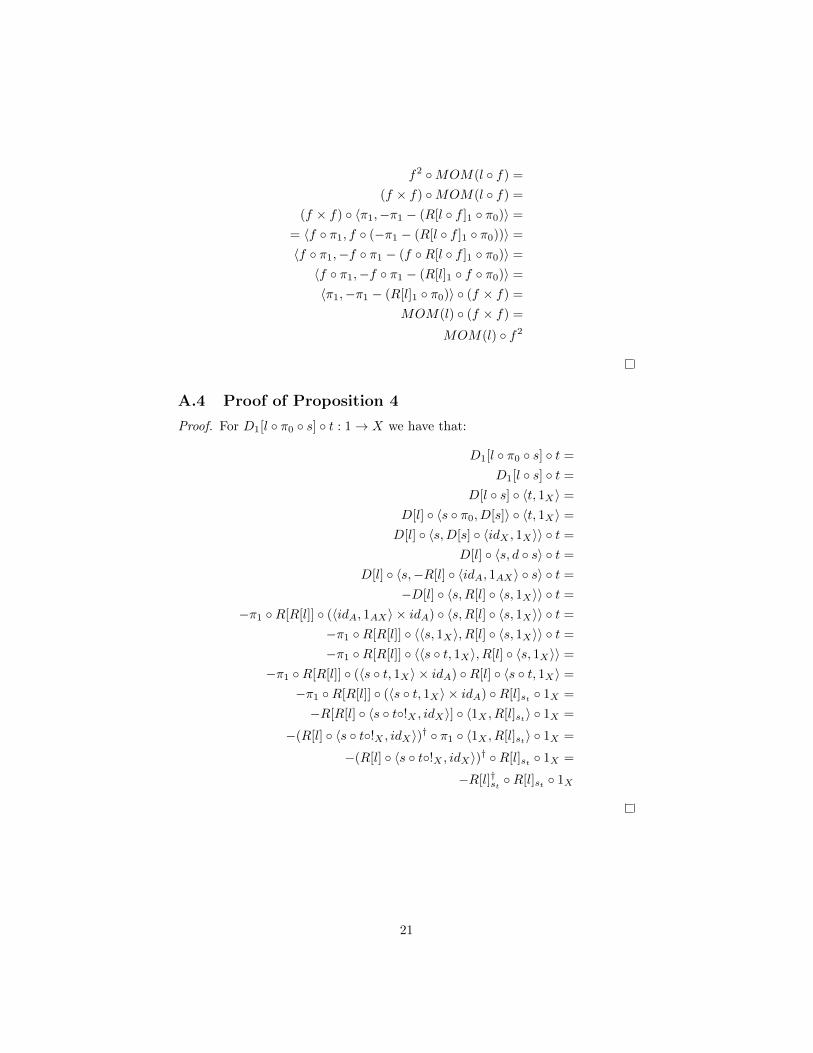
A.4 Proof of Proposition 4
Proof. For D1[l ◦ π0 ◦ s] ◦ t : 1→ X we have that: