25
Generating Simple and Complex Clinical Graphs using Efficient SAS/GRAPH ® Procedures Sakthivel S, Lead Biostatistician TAKE Solutions Global LLP, Chennai

Generating Simple and Complex Clinical Graphs using Efficient
SAS/GRAPH ® Procedures
Sakthivel S, Lead Biostatistician
TAKE Solutions Global LLP, Chennai

Agenda
• Introduction
• Statistical Graphics (SG) procedures - Power to
do more
• Graph Template Language (GTL) - Sanity for
SAS Graphics
• Delights for the day – Programming some
selective simple and complex Clinical Graphs
• Conclusion

Introduction
• The process of statistical interpretation and analysis of the clinical trial data can be made more effectively through graphical display of data along with descriptive and inferential statistics.
• In particular, variety of Clinical Graphs with different dimension of data visualization can be efficiently achieved through GTL and SG procedures.

"One graph is more effective than another if its
quantitative information can be decoded more
quickly and more easily by most observers." -
Naomi Robbins (2005)

SG Procedures – Power to do more
• ODS Graphics and the SG procedures introduces an exciting new way of producing graphs using SAS.
• With just a few lines of code, you can create a wide variety of high-quality graphs.
• Of the three major SG procedures (SGPLOT, SGPANEL, SGSCATTER), SGPLOT is the one that people will use most often.

GTL – Sanity for SAS Graphics
• Incorporates many automatic features such as label-
collision avoidance algorithms.
• Use state-of-the-art rendering technology with a wide
choice of output possibilities.
• GTL is more verbose but highly structured and flexible.
• Although many of tasks can be accomplished using the
SG procedures, those procedures do not provide many of
the advanced layout capabilities of GTL.
Delights for the day - Some selective simple and complex Clinical Graphs
ü Kaplan-Meier Plot - Time to event analysis
ü Line plot - Baseline and Post baseline by patient
ü Water-fall plot - Percent change from baseline reporting
ü Longitudinal plot - Mean (+/-) SD by treatment and
visit
ü Drug Exposure plot - by Treatment and RECIST
Overall response
ü Forest plot - Most frequent AE with Relative Risk

Basic Pre-requisites for any Graph
1. Be an architect of the Graph.
2. Identify x, y and group variable from the dataset.
3. Identify what are the plot statement are required to draw the
Graph.
4. Choose the attributes linestyle/pattern, markersymbol and color
for meaningful pictorial representation.
5. Decide the position of the legend and what exactly to be
presented in legend.
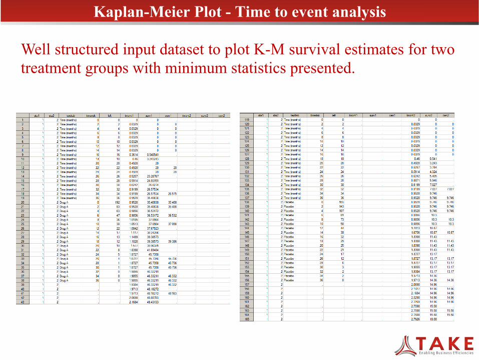
Kaplan-Meier Plot - Time to event analysis
Well structured input dataset to plot K-M survival estimates for two treatment groups with minimum statistics presented.
proc template; define statgraph kmplot; BeginGraph / border=false pad=0 designwidth=26.0cm designheight=17.5cm ; /*--- To plot titles and footnotes ---*/ entrytitle halign=left "CXYZ123 CSR"; entrytitle HALIGN = left " "; entrytitle HALIGN = center "Figure 14.3-2.2 (Page 1 of 1)"; entrytitle HALIGN = center "Time to first occurrence of new or worsening Hyperglycemic events, by treatment"; entrytitle HALIGN = center "Safety Set"; entrytitle HALIGN = center " "; entryfootnote HALIGN = left " "; entryfootnote HALIGN = left "- n represents the number of patients in the population with an uncensored event."; entryfootnote HALIGN = left "- Only patients with available baseline are included."; entryfootnote HALIGN = left " "; entryfootnote HALIGN = left "CXYZ123/report/pgm_saf/&pgmname..sas" halign=right "Version 1.0"; /*--- To plot censored symbols and text as legend ---*/ legendItem type=marker name="a_marker"/markerattrs=(color=green symbol=squarefilled) lineattrs=(color=green pattern = 1); legendItem type=marker name="p_marker"/markerattrs=(color=blue symbol=triangledownfilled)lineattrs=(color=blue pattern = 34); legendItem type=text name="indic" / text="Censoring Times" ; layout lattice/rows=2 columns=1 columndatarange=unionall rowweights=(.86 .14); layout overlay / xaxisopts=(label= "Time (months)" offsetmin=0 linearopts= (tickvaluepriority=true tickvaluelist=(0 2 4 6 8 10 12 14 16 18 20 22 24 26 28 30 32 34 36))) yaxisopts=(label="Probability (%) of event" linearopts=(viewmin=0 viewmax=100)); stepplot y=SURV1 x=tmont1/group=sta1 lineattrs = graphdata1(pattern = 1 color=green thickness=2) name="Survival1" ; scatterplot y=CEN1 x=tmont1/group=sta1 markerattrs=(symbol=squarefilled color=Green) legendlabel="q1" name="SCATTER1"; stepplot y=SURV2 x=tmont2/group=sta2 lineattrs = graphdata2(pattern = 34 color=blue thickness=1) name="Survival2" ; scatterplot y=CEN2 x=tmont2/group=sta2 markerattrs=(symbol=triangledownfilled color=Blue) legendlabel="q1"name="SCATTER2"; discretelegend "a_marker" "p_marker" "indic"/across=3 halign=right valign=0.3 autoitemsize=True location=inside border=false; discretelegend "Survival1" "SCATTER1" / merge=true halign=right valign=0.25 autoitemsize=True location=inside border= false; discretelegend "Survival2" "SCATTER2" / merge=true halign=right valign=0.2 autoitemsize=True location=inside border= false; layout gridded/columns=1 border=false autoalign=(BottomRight); entry halign=left " "; entry halign=left "Kaplan-Meier medians"; entry halign=left " Drug A: &medin1. months"; entry halign=left "Placebo: &medin2. months"; endlayout; endlayout; /*--- Table below the graph ---*/ cell; layout overlay / border=false walldisplay=none xaxisopts=(display=none linearopts=(viewmax=36
tickvaluesequence=(start=0 end=36 increment=2))) yaxisopts=(display=(tickvalues) type=discrete reverse=true); scatterplot x=timerisk y=texttab / markercharacter=left markercharacterattrs=GraphDataText; endlayout; cellheader; entry halign=left "No. of patients still at risk"; endcellheader; endcell; endlayout; EndGraph; end; quit; run; options orientation=landscape papersize='ISO A4' nodate nonumber nobyline; ods pdf file="CXYZ123/report/safety/KM2_TTOHYPE.pdf" style=graph dpi=300; ods listing close; /* Avoid .PNG creation in home drive*/ proc sgrender data=km1_ids template=kmplot; run; ods listing; ods pdf close;
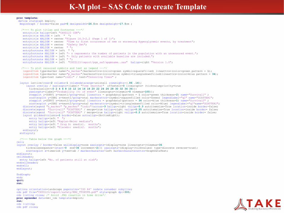
K-M plot – SAS Code to create Template
proc template; define statgraph kmplot; BeginGraph / border=false pad=0 designwidth=26.0cm designheight=17.5cm ; /*--- To plot titles and footnotes ---*/ entrytitle halign=left "CXYZ123 CSR"; entrytitle HALIGN = left " "; entrytitle HALIGN = center "Figure 14.3-2.2 (Page 1 of 1)"; entrytitle HALIGN = center "Time to first occurrence of new or worsening Hyperglycemic events, by treatment"; entrytitle HALIGN = center "Safety Set"; entrytitle HALIGN = center " "; entryfootnote HALIGN = left " "; entryfootnote HALIGN = left "- n represents the number of patients in the population with an uncensored event."; entryfootnote HALIGN = left "- Only patients with available baseline are included."; entryfootnote HALIGN = left " "; entryfootnote HALIGN = left "CXYZ123/report/pgm_saf/&pgmname..sas" halign=right "Version 1.0"; /*--- To plot censored symbols and text as legend ---*/ legendItem type=marker name="a_marker"/markerattrs=(color=green symbol=squarefilled) lineattrs=(color=green pattern = 1); legendItem type=marker name="p_marker"/markerattrs=(color=blue symbol=triangledownfilled)lineattrs=(color=blue pattern = 34); legendItem type=text name="indic" / text="Censoring Times" ;
layout lattice/rows=2 columns=1 columndatarange=unionall rowweights=(.86 .14); layout overlay / xaxisopts=(label= "Time (months)" offsetmin=0 linearopts= (tickvaluepriority=true tickvaluelist=(0 2 4 6 8 10 12 14 16 18 20 22 24 26 28 30 32 34 36))) yaxisopts=(label="Probability (%) of event" linearopts=(viewmin=0 viewmax=100)); stepplot y=SURV1 x=tmont1/group=sta1 lineattrs = graphdata1(pattern = 1 color=green thickness=2) name="Survival1" ; scatterplot y=CEN1 x=tmont1/group=sta1 markerattrs=(symbol=squarefilled color=Green) legendlabel="q1" name="SCATTER1"; stepplot y=SURV2 x=tmont2/group=sta2 lineattrs = graphdata2(pattern = 34 color=blue thickness=1) name="Survival2" ; scatterplot y=CEN2 x=tmont2/group=sta2 markerattrs=(symbol=triangledownfilled color=Blue) legendlabel="q1"name="SCATTER2"; discretelegend "a_marker" "p_marker" "indic"/across=3 halign=right valign=0.3 autoitemsize=True location=inside border=false; discretelegend "Survival1" "SCATTER1" / merge=true halign=right valign=0.25 autoitemsize=True location=inside border= false; discretelegend "Survival2" "SCATTER2" / merge=true halign=right valign=0.2 autoitemsize=True location=inside border= false; layout gridded/columns=1 border=false autoalign=(BottomRight); entry halign=left " "; entry halign=left "Kaplan-Meier medians"; entry halign=left " Drug A: &medin1. months"; entry halign=left "Placebo: &medin2. months"; endlayout; endlayout;
/*--- Table below the graph ---*/ cell; layout overlay / border=false walldisplay=none xaxisopts=(display=none linearopts=(viewmax=36
tickvaluesequence=(start=0 end=36 increment=2))) yaxisopts=(display=(tickvalues) type=discrete reverse=true); scatterplot x=timerisk y=texttab / markercharacter=left markercharacterattrs=GraphDataText; endlayout; cellheader; entry halign=left "No. of patients still at risk"; endcellheader; endcell; endlayout; EndGraph; end; quit; run; options orientation=landscape papersize='ISO A4' nodate nonumber nobyline; ods pdf file="CXYZ123/report/safety/KM2_TTOHYPE.pdf" style=graph dpi=300; ods listing close; /* Avoid .PNG creation in home drive*/ proc sgrender data=km1_ids template=kmplot; run; ods listing; ods pdf close;
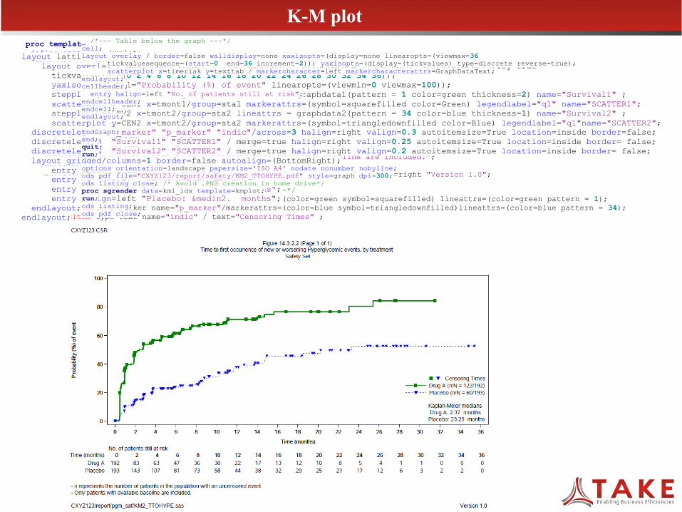
K-M plot
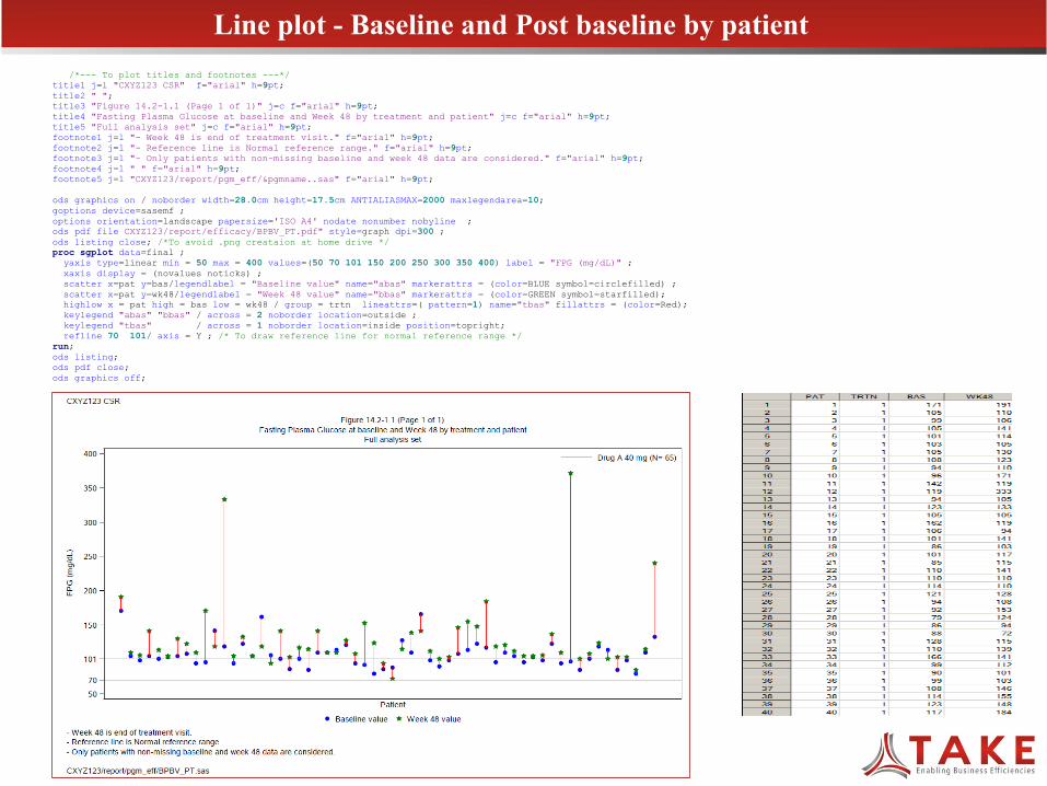
/*--- To plot titles and footnotes ---*/ title1 j=l "CXYZ123 CSR" f="arial" h=9pt; title2 " "; title3 "Figure 14.2-1.1 (Page 1 of 1)" j=c f="arial" h=9pt; title4 "Fasting Plasma Glucose at baseline and Week 48 by treatment and patient" j=c f="arial" h=9pt; title5 "Full analysis set" j=c f="arial" h=9pt; footnote1 j=l "- Week 48 is end of treatment visit." f="arial" h=9pt; footnote2 j=l "- Reference line is Normal reference range." f="arial" h=9pt; footnote3 j=l "- Only patients with non-missing baseline and week 48 data are considered." f="arial" h=9pt; footnote4 j=l " " f="arial" h=9pt; footnote5 j=l "CXYZ123/report/pgm_eff/&pgmname..sas" f="arial" h=9pt; ods graphics on / noborder width=28.0cm height=17.5cm ANTIALIASMAX=2000 maxlegendarea=10; goptions device=sasemf ; options orientation=landscape papersize='ISO A4' nodate nonumber nobyline ; ods pdf file CXYZ123/report/efficacy/BPBV_PT.pdf" style=graph dpi=300 ; ods listing close; /*To avoid .png creataion at home drive */ proc sgplot data=final ; yaxis type=linear min = 50 max = 400 values=(50 70 101 150 200 250 300 350 400) label = "FPG (mg/dL)" ; xaxis display = (novalues noticks) ; scatter x=pat y=bas/legendlabel = "Baseline value" name="abas" markerattrs = (color=BLUE symbol=circlefilled) ; scatter x=pat y=wk48/legendlabel = "Week 48 value" name="bbas" markerattrs = (color=GREEN symbol=starfilled); highlow x = pat high = bas low = wk48 / group = trtn lineattrs=( pattern=1) name="tbas" fillattrs = (color=Red); keylegend "abas" "bbas" / across = 2 noborder location=outside ; keylegend "tbas" / across = 1 noborder location=inside position=topright; refline 70 101/ axis = Y ; /* To draw reference line for normal reference range */ run; ods listing; ods pdf close; ods graphics off;
Line plot - Baseline and Post baseline by patient
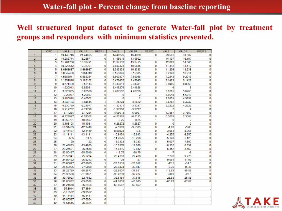
Well structured input dataset to generate Water-fall plot by treatment groups and responders with minimum statistics presented.
Water-fall plot - Percent change from baseline reporting
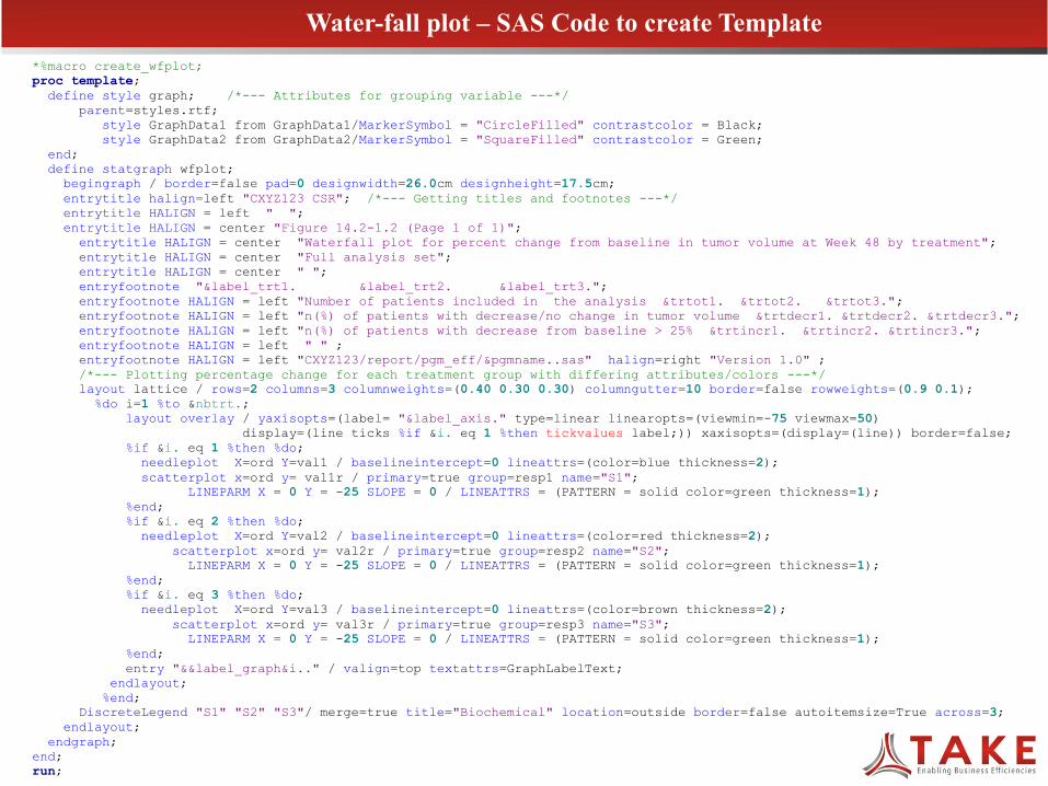
*%macro create_wfplot; proc template; define style graph; /*--- Attributes for grouping variable ---*/ parent=styles.rtf; style GraphData1 from GraphData1/MarkerSymbol = "CircleFilled" contrastcolor = Black; style GraphData2 from GraphData2/MarkerSymbol = "SquareFilled" contrastcolor = Green; end; define statgraph wfplot; begingraph / border=false pad=0 designwidth=26.0cm designheight=17.5cm; entrytitle halign=left "CXYZ123 CSR"; /*--- Getting titles and footnotes ---*/ entrytitle HALIGN = left " "; entrytitle HALIGN = center "Figure 14.2-1.2 (Page 1 of 1)"; entrytitle HALIGN = center "Waterfall plot for percent change from baseline in tumor volume at Week 48 by treatment"; entrytitle HALIGN = center "Full analysis set"; entrytitle HALIGN = center " "; entryfootnote "&label_trt1. &label_trt2. &label_trt3."; entryfootnote HALIGN = left "Number of patients included in the analysis &trtot1. &trtot2. &trtot3."; entryfootnote HALIGN = left "n(%) of patients with decrease/no change in tumor volume &trtdecr1. &trtdecr2. &trtdecr3."; entryfootnote HALIGN = left "n(%) of patients with decrease from baseline > 25% &trtincr1. &trtincr2. &trtincr3."; entryfootnote HALIGN = left " " ; entryfootnote HALIGN = left "CXYZ123/report/pgm_eff/&pgmname..sas" halign=right "Version 1.0" ; /*--- Plotting percentage change for each treatment group with differing attributes/colors ---*/ layout lattice / rows=2 columns=3 columnweights=(0.40 0.30 0.30) columngutter=10 border=false rowweights=(0.9 0.1); %do i=1 %to &nbtrt.; layout overlay / yaxisopts=(label= "&label_axis." type=linear linearopts=(viewmin=-75 viewmax=50) display=(line ticks %if &i. eq 1 %then tickvalues label;)) xaxisopts=(display=(line)) border=false; %if &i. eq 1 %then %do; needleplot X=ord Y=val1 / baselineintercept=0 lineattrs=(color=blue thickness=2); scatterplot x=ord y= val1r / primary=true group=resp1 name="S1"; LINEPARM X = 0 Y = -25 SLOPE = 0 / LINEATTRS = (PATTERN = solid color=green thickness=1); %end; %if &i. eq 2 %then %do; needleplot X=ord Y=val2 / baselineintercept=0 lineattrs=(color=red thickness=2); scatterplot x=ord y= val2r / primary=true group=resp2 name="S2"; LINEPARM X = 0 Y = -25 SLOPE = 0 / LINEATTRS = (PATTERN = solid color=green thickness=1); %end; %if &i. eq 3 %then %do; needleplot X=ord Y=val3 / baselineintercept=0 lineattrs=(color=brown thickness=2); scatterplot x=ord y= val3r / primary=true group=resp3 name="S3"; LINEPARM X = 0 Y = -25 SLOPE = 0 / LINEATTRS = (PATTERN = solid color=green thickness=1); %end; entry "&&label_graph&i.." / valign=top textattrs=GraphLabelText; endlayout; %end; DiscreteLegend "S1" "S2" "S3"/ merge=true title="Biochemical" location=outside border=false autoitemsize=True across=3; endlayout; endgraph; end; run;
Water-fall plot – SAS Code to create Template
*%macro create_wfplot; proc template; define style graph; /*--- Attributes for grouping variable ---*/ parent=styles.rtf; style GraphData1 from GraphData1/MarkerSymbol = "CircleFilled" contrastcolor = Black; style GraphData2 from GraphData2/MarkerSymbol = "SquareFilled" contrastcolor = Green; end; define statgraph wfplot; begingraph / border=false pad=0 designwidth=26.0cm designheight=17.5cm; entrytitle halign=left "CXYZ123 CSR"; /*--- Getting titles and footnotes ---*/ entrytitle HALIGN = left " "; entrytitle HALIGN = center "Figure 14.2-1.2 (Page 1 of 1)"; entrytitle HALIGN = center "Waterfall plot for percent change from baseline in tumor volume at Week 48 by treatment"; entrytitle HALIGN = center "Full analysis set"; entrytitle HALIGN = center " "; entryfootnote "&label_trt1. &label_trt2. &label_trt3."; entryfootnote HALIGN = left "Number of patients included in the analysis &trtot1. &trtot2. &trtot3."; entryfootnote HALIGN = left "n(%) of patients with decrease/no change in tumor volume &trtdecr1. &trtdecr2. &trtdecr3."; entryfootnote HALIGN = left "n(%) of patients with decrease from baseline > 25% &trtincr1. &trtincr2. &trtincr3."; entryfootnote HALIGN = left " " ; entryfootnote HALIGN = left "CXYZ123/report/pgm_eff/&pgmname..sas" halign=right "Version 1.0" ;
/*--- Plotting percentage change for each treatment group with differing attributes/colors ---*/ layout lattice / rows=2 columns=3 columnweights=(0.40 0.30 0.30) columngutter=10 border=false rowweights=(0.9 0.1); %do i=1 %to &nbtrt.; layout overlay / yaxisopts=(label= "&label_axis." type=linear linearopts=(viewmin=-75 viewmax=50) display=(line ticks %if &i. eq 1 %then tickvalues label;)) xaxisopts=(display=(line)) border=false; %if &i. eq 1 %then %do; needleplot X=ord Y=val1 / baselineintercept=0 lineattrs=(color=blue thickness=2); scatterplot x=ord y= val1r / primary=true group=resp1 name="S1"; LINEPARM X = 0 Y = -25 SLOPE = 0 / LINEATTRS = (PATTERN = solid color=green thickness=1); %end; %if &i. eq 2 %then %do; needleplot X=ord Y=val2 / baselineintercept=0 lineattrs=(color=red thickness=2); scatterplot x=ord y= val2r / primary=true group=resp2 name="S2"; LINEPARM X = 0 Y = -25 SLOPE = 0 / LINEATTRS = (PATTERN = solid color=green thickness=1); %end; %if &i. eq 3 %then %do; needleplot X=ord Y=val3 / baselineintercept=0 lineattrs=(color=brown thickness=2); scatterplot x=ord y= val3r / primary=true group=resp3 name="S3"; LINEPARM X = 0 Y = -25 SLOPE = 0 / LINEATTRS = (PATTERN = solid color=green thickness=1); %end; entry "&&label_graph&i.." / valign=top textattrs=GraphLabelText; endlayout; %end; DiscreteLegend "S1" "S2" "S3"/ merge=true title="Biochemical" location=outside border=false autoitemsize=True across=3; endlayout; endgraph; end; run;
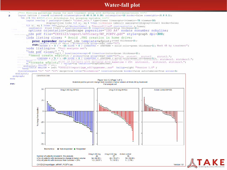
options orientation=landscape papersize='ISO A4' nodate nonumber nobyline; ods pdf file="CXYZ123/report/efficacy/WF_PCBTV.pdf" style=graph dpi=300; ods listing close; * Avoid .PNG creation in home drive; proc sgrender data=wf_ids template=wfplot; run; ods listing; ods pdf close; *%mend create_wfplot; *%create_wfplot;
Water-fall plot
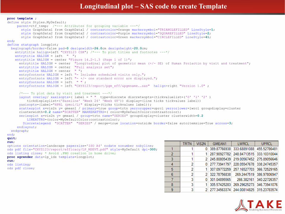
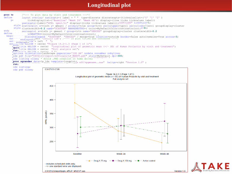
proc template ; define style Styles.MyDefault; parent=rtf_temp; /*--- Attributes for grouping variable ---*/ style GraphData1 from GraphData1 / contrastcolor=Orange markersymbol="TRIANGLEFILLED" LineStyle=1; style GraphData2 from GraphData2 / contrastcolor=Purple markersymbol="SQUAREFILLED" LineStyle=2; style GraphData3 from GraphData3 / contrastcolor=Green markersymbol="CIRCLEFILLED" LineStyle=41; end; define statgraph longplot; begingraph/border=false pad=0 designwidth=26.0cm designheight=20.0cm; entrytitle halign=left "CXYZ123 CSR"; /*--- To plot titles and footnotes ---*/ entrytitle HALIGN = left " "; entrytitle HALIGN = center "Figure 14.2-1.3 (Page 1 of 1)"; entrytitle HALIGN = center "Longitudinal plot of geometric mean (+/- SE) of Human Prolactin by visit and treatment"; entrytitle HALIGN = center "Full analysis set"; entrytitle HALIGN = center " "; entryfootnote HALIGN = left "- Includes scheduled visits only."; entryfootnote HALIGN = left "- +/- one standard error are displayed."; entryfootnote HALIGN = left " " ; entryfootnote HALIGN = left "CXYZ123/report/pgm_eff/&pgmname..sas" halign=right "Version 1.0" ;
/*--- To plot data by visit and treatment ---*/ layout overlay/ xaxisopts=( label = " " type=discrete discreteopts=(tickvaluelist=('0' '1' '2' ) tickdisplaylist=('Baseline' 'Week 24' 'Week 48')) display=(line ticks tickvalues label)) yaxisopts=(label="HPRL (pmol/L)" display=(ticks tickvalues label));
scatterplot x=vis2n y= gmean1 / primary=true group=trtn yerrorupper=uprcl yerrorlower=lwrcl groupdisplay=cluster clusterwidth=0.2 name="SCATTER" MARKERATTRS=( color=MyDefaultColor:contrastcolor);
seriesplot x=vis2n y= gmean1 / group=trtn name="SERIES" groupdisplay=cluster clusterwidth=0.2 LINEATTRS=(color=MyDefaultColor:contrastcolor); Discretelegend "SCATTER" "SERIES" / merge=true location=outside border=false autoitemsize=True across=3; endlayout; endgraph; end; quit; run; options orientation=landscape papersize='ISO A4' nodate nonumber nobyline; ods pdf file="CXYZ123/report/efficacy/LP_MSEVT.pdf" style=MyDefault dpi=300; ods listing close; * Avoid .PNG creation in home drive; proc sgrender data=lp_ids template=longplot; run; ods listing; ods pdf close;
Longitudinal plot – SAS code to create Template
proc template ; define style Styles.MyDefault; parent=rtf_temp; /*--- Attributes for grouping variable ---*/ style GraphData1 from GraphData1 / contrastcolor=Orange markersymbol="TRIANGLEFILLED" LineStyle=1; style GraphData2 from GraphData2 / contrastcolor=Purple markersymbol="SQUAREFILLED" LineStyle=2; style GraphData3 from GraphData3 / contrastcolor=Green markersymbol="CIRCLEFILLED" LineStyle=41; end; define statgraph longplot; begingraph/border=false pad=0 designwidth=26.0cm designheight=20.0cm; entrytitle halign=left "CXYZ123 CSR"; /*--- To plot titles and footnotes ---*/ entrytitle HALIGN = left " "; entrytitle HALIGN = center "Figure 14.2-1.3 (Page 1 of 1)"; entrytitle HALIGN = center "Longitudinal plot of geometric mean (+/- SE) of Human Prolactin by visit and treatment"; entrytitle HALIGN = center "Full analysis set"; entrytitle HALIGN = center " "; entryfootnote HALIGN = left "- Includes scheduled visits only."; entryfootnote HALIGN = left "- +/- one standard error are displayed."; entryfootnote HALIGN = left " " ; entryfootnote HALIGN = left "CXYZ123/report/pgm_eff/&pgmname..sas" halign=right "Version 1.0" ;
/*--- To plot data by visit and treatment ---*/ layout overlay/ xaxisopts=( label = " " type=discrete discreteopts=(tickvaluelist=('0' '1' '2' ) tickdisplaylist=('Baseline' 'Week 24' 'Week 48')) display=(line ticks tickvalues label)) yaxisopts=(label="HPRL (pmol/L)" display=(ticks tickvalues label));
scatterplot x=vis2n y= gmean1 / primary=true group=trtn yerrorupper=uprcl yerrorlower=lwrcl groupdisplay=cluster clusterwidth=0.2 name="SCATTER" MARKERATTRS=( color=MyDefaultColor:contrastcolor);
seriesplot x=vis2n y= gmean1 / group=trtn name="SERIES" groupdisplay=cluster clusterwidth=0.2 LINEATTRS=(color=MyDefaultColor:contrastcolor); Discretelegend "SCATTER" "SERIES" / merge=true location=outside border=false autoitemsize=True across=3; endlayout; endgraph; end; quit; run; options orientation=landscape papersize='ISO A4' nodate nonumber nobyline; ods pdf file="CXYZ123/report/efficacy/LP_MSEVT.pdf" style=MyDefault dpi=300; ods listing close; * Avoid .PNG creation in home drive; proc sgrender data=lp_ids template=longplot; run; ods listing; ods pdf close;
Longitudinal plot
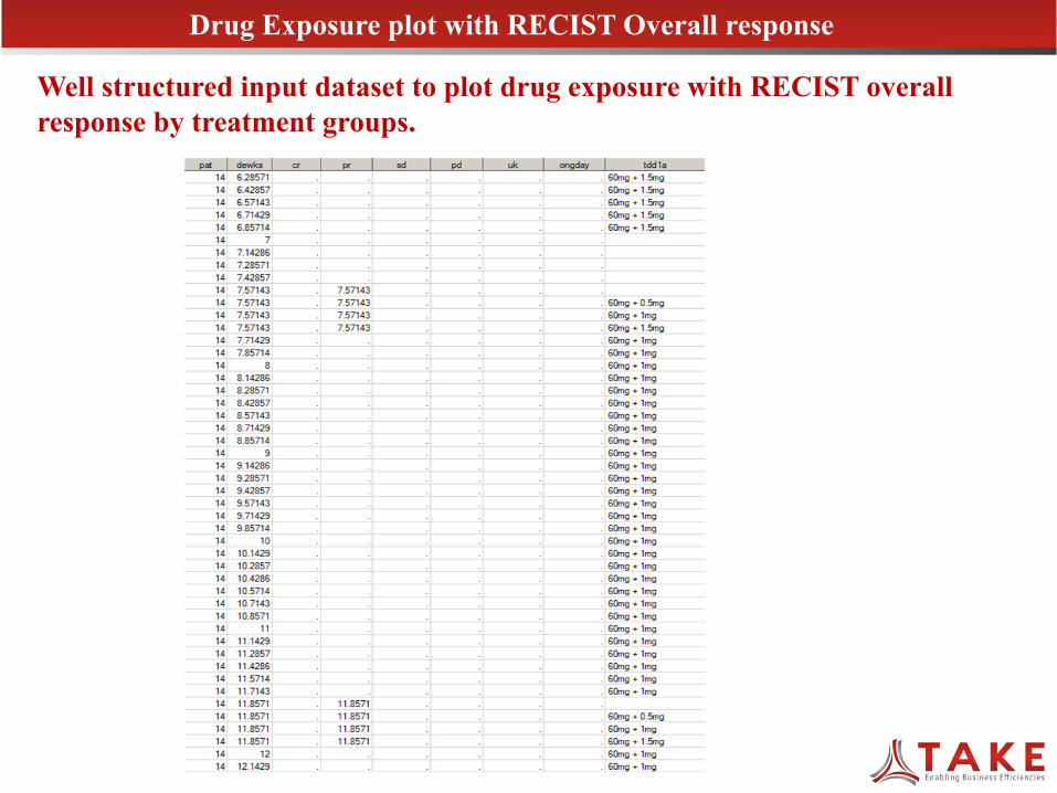
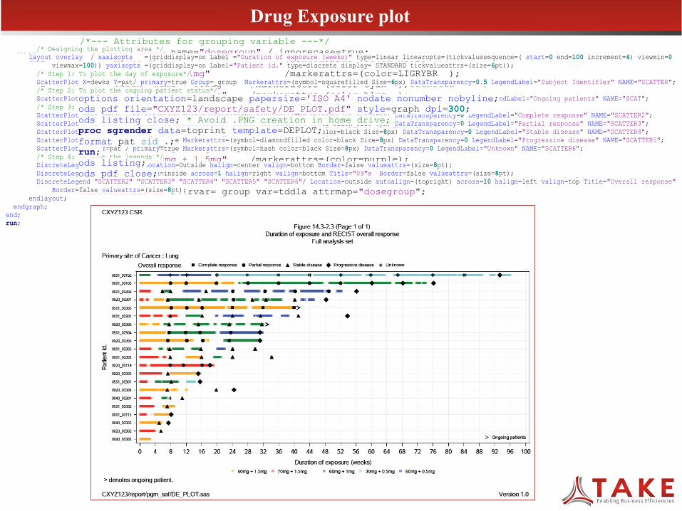
Well structured input dataset to plot drug exposure with RECIST overall response by treatment groups.
Drug Exposure plot with RECIST Overall response
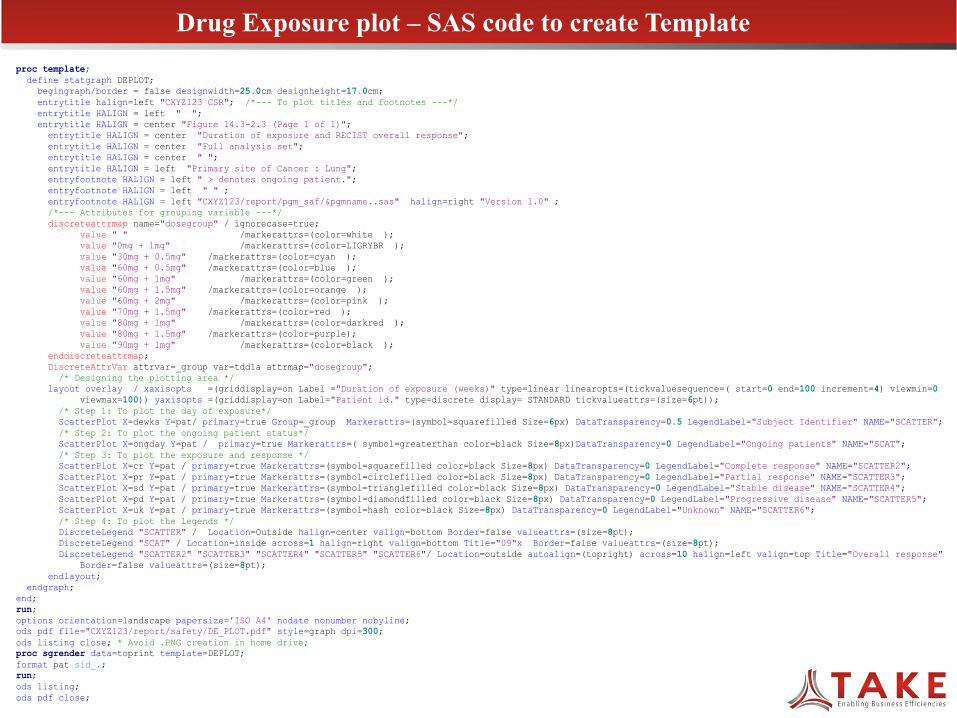
proc template; define statgraph DEPLOT; begingraph/border = false designwidth=25.0cm designheight=17.0cm; entrytitle halign=left "CXYZ123 CSR"; /*--- To plot titles and footnotes ---*/ entrytitle HALIGN = left " "; entrytitle HALIGN = center "Figure 14.3-2.3 (Page 1 of 1)"; entrytitle HALIGN = center "Duration of exposure and RECIST overall response"; entrytitle HALIGN = center "Full analysis set"; entrytitle HALIGN = center " "; entrytitle HALIGN = left "Primary site of Cancer : Lung"; entryfootnote HALIGN = left " > denotes ongoing patient."; entryfootnote HALIGN = left " " ; entryfootnote HALIGN = left "CXYZ123/report/pgm_saf/&pgmname..sas" halign=right "Version 1.0" ; /*--- Attributes for grouping variable ---*/ discreteattrmap name="dosegroup" / ignorecase=true; value " " /markerattrs=(color=white ); value "0mg + 1mg" /markerattrs=(color=LIGRYBR ); value "30mg + 0.5mg" /markerattrs=(color=cyan ); value "60mg + 0.5mg" /markerattrs=(color=blue ); value "60mg + 1mg" /markerattrs=(color=green ); value "60mg + 1.5mg" /markerattrs=(color=orange ); value "60mg + 2mg" /markerattrs=(color=pink ); value "70mg + 1.5mg" /markerattrs=(color=red ); value "80mg + 1mg" /markerattrs=(color=darkred ); value "80mg + 1.5mg" /markerattrs=(color=purple); value "90mg + 1mg" /markerattrs=(color=black ); enddiscreteattrmap; DiscreteAttrVar attrvar=_group var=tdd1a attrmap="dosegroup"; /* Designing the plotting area */ layout overlay / xaxisopts =(griddisplay=on Label ="Duration of exposure (weeks)" type=linear linearopts=(tickvaluesequence=( start=0 end=100 increment=4) viewmin=0
viewmax=100)) yaxisopts =(griddisplay=on Label="Patient id." type=discrete display= STANDARD tickvalueattrs=(size=6pt)); /* Step 1: To plot the day of exposure*/ ScatterPlot X=dewks Y=pat/ primary=true Group=_group Markerattrs=(symbol=squarefilled Size=6px) DataTransparency=0.5 LegendLabel="Subject Identifier" NAME="SCATTER"; /* Step 2: To plot the ongoing patient status*/ ScatterPlot X=ongday Y=pat / primary=true Markerattrs=( symbol=greaterthan color=black Size=8px)DataTransparency=0 LegendLabel="Ongoing patients" NAME="SCAT"; /* Step 3: To plot the exposure and response */ ScatterPlot X=cr Y=pat / primary=true Markerattrs=(symbol=squarefilled color=black Size=8px) DataTransparency=0 LegendLabel="Complete response" NAME="SCATTER2"; ScatterPlot X=pr Y=pat / primary=true Markerattrs=(symbol=circlefilled color=black Size=8px) DataTransparency=0 LegendLabel="Partial response" NAME="SCATTER3"; ScatterPlot X=sd Y=pat / primary=true Markerattrs=(symbol=trianglefilled color=black Size=8px) DataTransparency=0 LegendLabel="Stable disease" NAME="SCATTER4"; ScatterPlot X=pd Y=pat / primary=true Markerattrs=(symbol=diamondfilled color=black Size=8px) DataTransparency=0 LegendLabel="Progressive disease" NAME="SCATTER5"; ScatterPlot X=uk Y=pat / primary=true Markerattrs=(symbol=hash color=black Size=8px) DataTransparency=0 LegendLabel="Unknown" NAME="SCATTER6"; /* Step 4: To plot the legends */ DiscreteLegend "SCATTER" / Location=Outside halign=center valign=bottom Border=false valueattrs=(size=8pt); DiscreteLegend "SCAT" / Location=inside across=1 halign=right valign=bottom Title="09"x Border=false valueattrs=(size=8pt); DiscreteLegend "SCATTER2" "SCATTER3" "SCATTER4" "SCATTER5" "SCATTER6"/ Location=outside autoalign=(topright) across=10 halign=left valign=top Title="Overall response" Border=false valueattrs=(size=8pt); endlayout; endgraph; end; run; options orientation=landscape papersize='ISO A4' nodate nonumber nobyline; ods pdf file="CXYZ123/report/safety/DE_PLOT.pdf" style=graph dpi=300; ods listing close; * Avoid .PNG creation in home drive; proc sgrender data=toprint template=DEPLOT; format pat sid_.; run; ods listing; ods pdf close;
Drug Exposure plot – SAS code to create Template
proc template; define statgraph DEPLOT; begingraph/border = false designwidth=25.0cm designheight=17.0cm; entrytitle halign=left "CXYZ123 CSR"; /*--- To plot titles and footnotes ---*/ entrytitle HALIGN = left " "; entrytitle HALIGN = center "Figure 14.3-2.3 (Page 1 of 1)"; entrytitle HALIGN = center "Duration of exposure and RECIST overall response"; entrytitle HALIGN = center "Full analysis set"; entrytitle HALIGN = center " "; entrytitle HALIGN = left "Primary site of Cancer : Lung"; entryfootnote HALIGN = left " > denotes ongoing patient."; entryfootnote HALIGN = left " " ; entryfootnote HALIGN = left "CXYZ123/report/pgm_saf/&pgmname..sas" halign=right "Version 1.0" ;
/*--- Attributes for grouping variable ---*/ discreteattrmap name="dosegroup" / ignorecase=true; value " " /markerattrs=(color=white ); value "0mg + 1mg" /markerattrs=(color=LIGRYBR ); value "30mg + 0.5mg" /markerattrs=(color=cyan ); value "60mg + 0.5mg" /markerattrs=(color=blue ); value "60mg + 1mg" /markerattrs=(color=green ); value "60mg + 1.5mg" /markerattrs=(color=orange ); value "60mg + 2mg" /markerattrs=(color=pink ); value "70mg + 1.5mg" /markerattrs=(color=red ); value "80mg + 1mg" /markerattrs=(color=darkred ); value "80mg + 1.5mg" /markerattrs=(color=purple); value "90mg + 1mg" /markerattrs=(color=black ); enddiscreteattrmap; DiscreteAttrVar attrvar=_group var=tdd1a attrmap="dosegroup";
/* Designing the plotting area */ layout overlay / xaxisopts =(griddisplay=on Label ="Duration of exposure (weeks)" type=linear linearopts=(tickvaluesequence=( start=0 end=100 increment=4) viewmin=0
viewmax=100)) yaxisopts =(griddisplay=on Label="Patient id." type=discrete display= STANDARD tickvalueattrs=(size=6pt)); /* Step 1: To plot the day of exposure*/ ScatterPlot X=dewks Y=pat/ primary=true Group=_group Markerattrs=(symbol=squarefilled Size=6px) DataTransparency=0.5 LegendLabel="Subject Identifier" NAME="SCATTER"; /* Step 2: To plot the ongoing patient status*/ ScatterPlot X=ongday Y=pat / primary=true Markerattrs=( symbol=greaterthan color=black Size=8px)DataTransparency=0 LegendLabel="Ongoing patients" NAME="SCAT"; /* Step 3: To plot the exposure and response */ ScatterPlot X=cr Y=pat / primary=true Markerattrs=(symbol=squarefilled color=black Size=8px) DataTransparency=0 LegendLabel="Complete response" NAME="SCATTER2"; ScatterPlot X=pr Y=pat / primary=true Markerattrs=(symbol=circlefilled color=black Size=8px) DataTransparency=0 LegendLabel="Partial response" NAME="SCATTER3"; ScatterPlot X=sd Y=pat / primary=true Markerattrs=(symbol=trianglefilled color=black Size=8px) DataTransparency=0 LegendLabel="Stable disease" NAME="SCATTER4"; ScatterPlot X=pd Y=pat / primary=true Markerattrs=(symbol=diamondfilled color=black Size=8px) DataTransparency=0 LegendLabel="Progressive disease" NAME="SCATTER5"; ScatterPlot X=uk Y=pat / primary=true Markerattrs=(symbol=hash color=black Size=8px) DataTransparency=0 LegendLabel="Unknown" NAME="SCATTER6"; /* Step 4: To plot the legends */ DiscreteLegend "SCATTER" / Location=Outside halign=center valign=bottom Border=false valueattrs=(size=8pt); DiscreteLegend "SCAT" / Location=inside across=1 halign=right valign=bottom Title="09"x Border=false valueattrs=(size=8pt); DiscreteLegend "SCATTER2" "SCATTER3" "SCATTER4" "SCATTER5" "SCATTER6"/ Location=outside autoalign=(topright) across=10 halign=left valign=top Title="Overall response" Border=false valueattrs=(size=8pt); endlayout; endgraph; end; run;
options orientation=landscape papersize='ISO A4' nodate nonumber nobyline; ods pdf file="CXYZ123/report/safety/DE_PLOT.pdf" style=graph dpi=300; ods listing close; * Avoid .PNG creation in home drive; proc sgrender data=toprint template=DEPLOT; format pat sid_.; run; ods listing; ods pdf close;
Drug Exposure plot
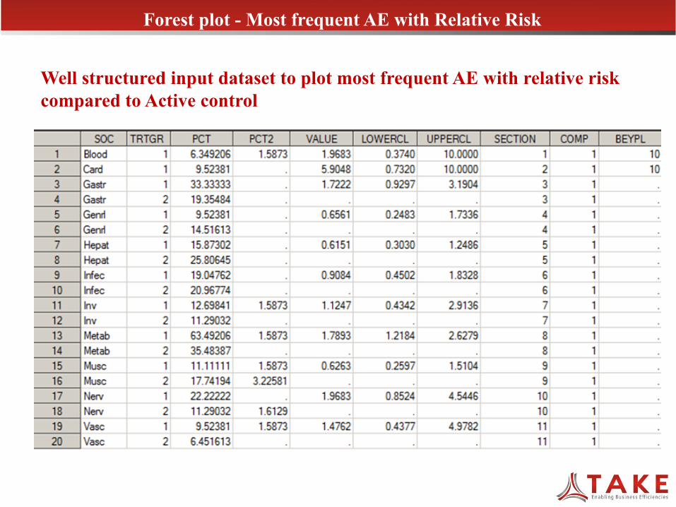
Well structured input dataset to plot most frequent AE with relative risk compared to Active control
Forest plot - Most frequent AE with Relative Risk
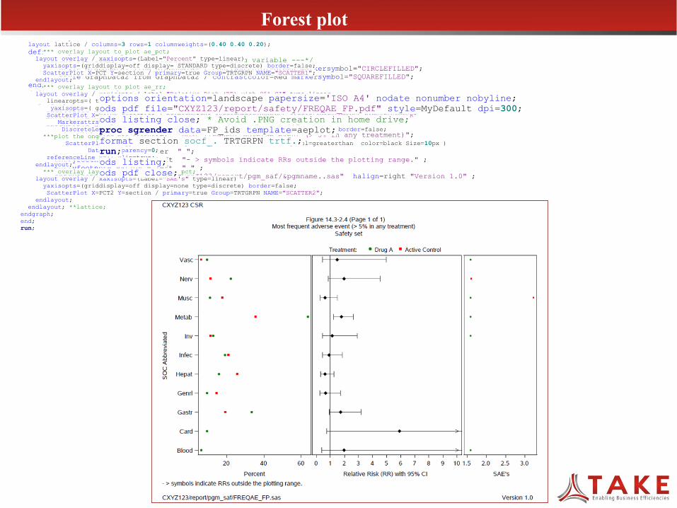
proc template; define style Styles.MyDefault; parent=rtf_temp; /*--- Attributes for grouping variable ---*/ style GraphData1 from GraphData1 / contrastcolor=Green markersymbol="CIRCLEFILLED"; style GraphData2 from GraphData2 / contrastcolor=Red markersymbol="SQUAREFILLED"; end; define statgraph aeplot; begingraph/border = false designwidth=25.0cm designheight=20.0cm; entrytitle halign=left "CXYZ123 CSR"; /*--- To plot titles and footnotes ---*/ entrytitle HALIGN = left " "; entrytitle HALIGN = center "Figure 14.3-2.4 (Page 1 of 1)"; entrytitle HALIGN = center "Most frequent adverse event (> 5% in any treatment)"; entrytitle HALIGN = center "Safety set"; entrytitle HALIGN = center " "; entryfootnote HALIGN = left "- > symbols indicate RRs outside the plotting range." ; entryfootnote HALIGN = left " " ; entryfootnote HALIGN = left "CXYZ123/report/pgm_saf/&pgmname..sas" halign=right "Version 1.0" ; layout lattice / columns=3 rows=1 columnweights=(0.40 0.40 0.20);
*** overlay layout to plot ae_pct; layout overlay / xaxisopts=(Label="Percent" type=linear) yaxisopts=(griddisplay=off display= STANDARD type=discrete) border=false; ScatterPlot X=PCT Y=section / primary=true Group=TRTGRPN NAME="SCATTER1"; endlayout;
*** overlay layout to plot ae_rr; layout overlay / xaxisopts=( Label="Relative Risk (RR) with 95% CI" type=linear linearopts=( tickvaluelist=( 0 1 2 3 4 5 6 7 8 9 10) viewmin=0 viewmax=10)) yaxisopts=( griddisplay=off display=none) border=false; ScatterPlot X=VALUE Y=section / primary=true XErrorUpper=UPPERCL XErrorLower=LOWERCL NAME="SCATTER" Markerattrs=(symbol=diamondfilled color=black Size=8px); DiscreteLegend "SCATTER1"/ Location=outside valign=top title="Treatment:" border=false;
***plot the ongoing pts status* ScatterPlot X=beypl Y=section / primary=true Markerattrs=( symbol=greaterthan color=black Size=10px ) DataTransparency=0; referenceLine x=1/ clip=true; endlayout;
*** overlay layout codes to plot Sae_pct; layout overlay / xaxisopts=(Label="SAE's" type=linear) yaxisopts=(griddisplay=off display=none type=discrete) border=false; ScatterPlot X=PCT2 Y=section / primary=true Group=TRTGRPN NAME="SCATTER2"; endlayout; endlayout; **lattice; endgraph; end; run; options orientation=landscape papersize='ISO A4' nodate nonumber nobyline; ods pdf file="CXYZ123/report/safety/FREQAE_FP.pdf" style=MyDefault dpi=300; ods listing close; * Avoid .PNG creation in home drive; proc sgrender data=FP_ids template=aeplot; format section socf_. TRTGRPN trtf.; run; ods listing; ods pdf close;
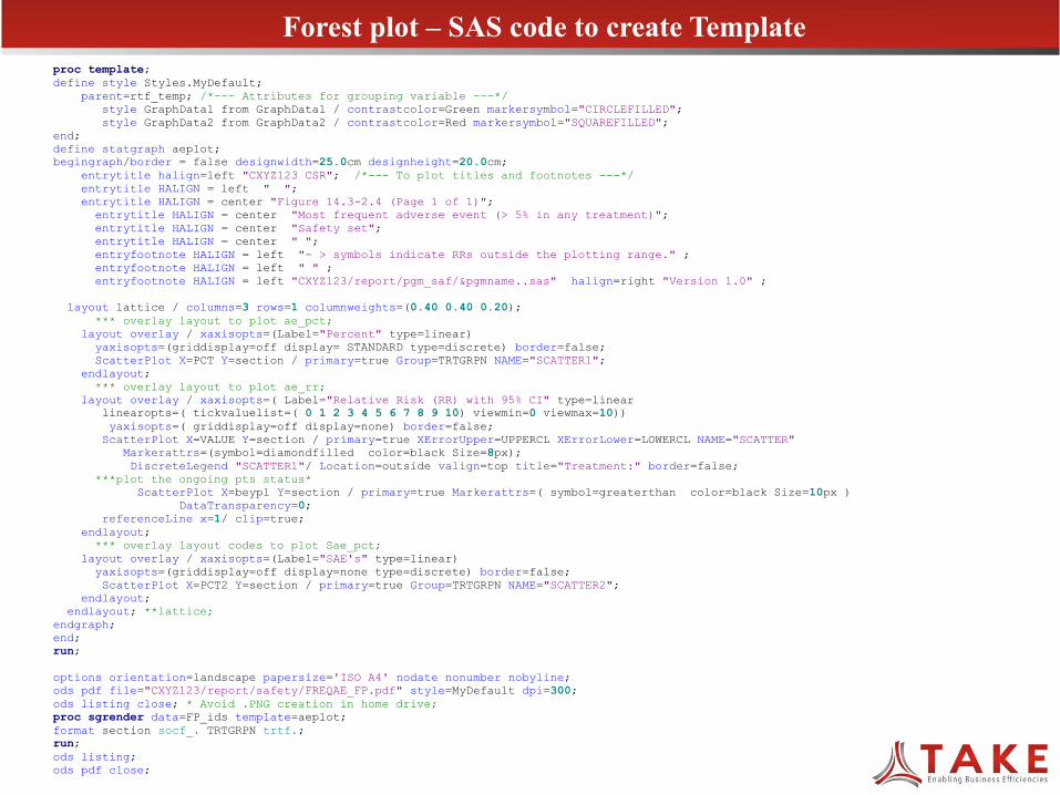
Forest plot – SAS code to create Template
proc template; define style Styles.MyDefault; parent=rtf_temp; /*--- Attributes for grouping variable ---*/ style GraphData1 from GraphData1 / contrastcolor=Green markersymbol="CIRCLEFILLED"; style GraphData2 from GraphData2 / contrastcolor=Red markersymbol="SQUAREFILLED"; end; define statgraph aeplot; begingraph/border = false designwidth=25.0cm designheight=20.0cm; entrytitle halign=left "CXYZ123 CSR"; /*--- To plot titles and footnotes ---*/ entrytitle HALIGN = left " "; entrytitle HALIGN = center "Figure 14.3-2.4 (Page 1 of 1)"; entrytitle HALIGN = center "Most frequent adverse event (> 5% in any treatment)"; entrytitle HALIGN = center "Safety set"; entrytitle HALIGN = center " "; entryfootnote HALIGN = left "- > symbols indicate RRs outside the plotting range." ; entryfootnote HALIGN = left " " ; entryfootnote HALIGN = left "CXYZ123/report/pgm_saf/&pgmname..sas" halign=right "Version 1.0" ;
layout lattice / columns=3 rows=1 columnweights=(0.40 0.40 0.20); *** overlay layout to plot ae_pct;
layout overlay / xaxisopts=(Label="Percent" type=linear) yaxisopts=(griddisplay=off display= STANDARD type=discrete) border=false; ScatterPlot X=PCT Y=section / primary=true Group=TRTGRPN NAME="SCATTER1"; endlayout;
*** overlay layout to plot ae_rr; layout overlay / xaxisopts=( Label="Relative Risk (RR) with 95% CI" type=linear linearopts=( tickvaluelist=( 0 1 2 3 4 5 6 7 8 9 10) viewmin=0 viewmax=10)) yaxisopts=( griddisplay=off display=none) border=false; ScatterPlot X=VALUE Y=section / primary=true XErrorUpper=UPPERCL XErrorLower=LOWERCL NAME="SCATTER" Markerattrs=(symbol=diamondfilled color=black Size=8px); DiscreteLegend "SCATTER1"/ Location=outside valign=top title="Treatment:" border=false;
***plot the ongoing pts status* ScatterPlot X=beypl Y=section / primary=true Markerattrs=( symbol=greaterthan color=black Size=10px ) DataTransparency=0; referenceLine x=1/ clip=true; endlayout;
*** overlay layout codes to plot Sae_pct; layout overlay / xaxisopts=(Label="SAE's" type=linear) yaxisopts=(griddisplay=off display=none type=discrete) border=false; ScatterPlot X=PCT2 Y=section / primary=true Group=TRTGRPN NAME="SCATTER2"; endlayout; endlayout; **lattice; endgraph; end; run;
options orientation=landscape papersize='ISO A4' nodate nonumber nobyline; ods pdf file="CXYZ123/report/safety/FREQAE_FP.pdf" style=MyDefault dpi=300; ods listing close; * Avoid .PNG creation in home drive; proc sgrender data=FP_ids template=aeplot; format section socf_. TRTGRPN trtf.; run; ods listing; ods pdf close;
Forest plot

Conclusion
ü The SG procedures and the GTL provide an efficient way of creating high-quality graphs quickly and with minimal programming effort.
ü Programming of any complex graphs can be made simple through the presented procedures using no more than a page of code because of well-structured built-in syntax supported by statements.
ü Surprisingly, no special coding or annotation is required.