Generating Synthetic Web Request Streams

S.R.Sarangi, P.N.Sireesh, S.P.Pal Department of Computer Science and Engineering

Indian Institute of Technology, Kharagpur, 721302, INDIA Email: spp@cse.iitkgp.ernet.in

Abstract

Synthetic web request streams find use in various fields. They can be used to evaluate web-caching algorithms, to evaluate the efficiency of network topologies and to plan future networks. This paper uses several empirically observed models of WAN traffic to create a realistic web request stream generator. The generator produces page requests matching empirical measurements of (a) relative file popularity and (b) temporal locality. An efficient algorithm is proposed to generate web request traces. The properties of the trace thus generated are identical to those of the empirically observed distributions. This method is scalable to a large number of requests and pages as its worst-case complexity is a linear function of the number of requests and a slowly growing function of the number of pages.

1. Introduction

The World Wide Web is assuming an increasingly important place in modern society. It has become a major source of information and entertainment. Financial transactions worth millions of dollars are being carried out over the web. Everyday millions of people logon to the net to check their e-mail and to get information about world affairs. The Internet has basically pervaded every aspect of human society. Improving the performance of the web has become a very important issue. Significant improvements have been realized in the performance of the web due to the incorporation of newer network protocols and web-caching strategies, leading to better quality of service to millions of users. For evaluation of such protocols and strategies a realistic network environment must be created. Simulation is a natural scientific method in this direction. Several researchers have built WAN simulators that can mimic wide area traffic. They test their algorithms and protocols on these simulators. The simulators used by them are of two types. The first type is called a “Trace based” simulator. Web traces are collected from links and stored in files. The simulator reads these files and generates the web workload. This approach is slow because it involves file operations. It is also restricted since it is dependent on datasets collected prior to the simulation. The second approach generates web requests according to analytic models. Their properties match empirically observed models of traffic.

Nowadays research focuses on simulators based on analytical models. Such simulators are fast, scalable and easy to use. They do not need collection of massive data sets. To build such simulators researchers have identified several characteristics of web requests. Analytical models have been proposed to model these characteristics. Simulators try to incorporate one or more of these observed characteristics. Here is a brief summary of the work done in this field.

1

1.1 Summary of Previous Work

Several studies have been carried out on web traces [1, 2, 3]. They suggest the following properties of web request streams.

a) File Sizes: The file sizes on a web server follow a heavy tailed distribution. Such distributions are well described by the Pareto distribution. The cumulative distribution function of this distribution is given by:

F(x) = 1 - x-β 0 < β < 2 (1.1.1) Such distributions are characterized by their infinite variance.

b) Request sizes: The request size distribution is also seen to follow a heavy tailed property. The request size distribution is the distribution of the sizes of the files actually transferred over the network. This is different from the server file size distribution. This is because the same file can be requested multiple times.

c) Popularity: The popularity of web pages is observed to follow the Zipf’s law. The Zipf’s law states that the popularity of the ith most popular page varies inversely with i. Stated mathematically the probability mass function p is given by: Error! Bookmark not

defined. p(i) = iΩ

(1.1.2)

d) Temporal locality: This property refers to the probability that if a given a page has been requested, it will be requested again in the near future. To characterize this the stack-distance model has been proposed.

The stack-distance model can be explained as follows. Given that the pages are organized in the form of a stack <p1, p2, .…. pn>. Suppose the next request is for the page pi. Then the stack-distance di for this request is i. Stack distance basically measures the depth within the stack where the next request is found. After this page i is moved to the top of the stack, the configuration of the new stack is <pi, p1, p2,..... pi-1, pi+1, .... pn>.

Thus given the configuration of the initial stack, a stream of stack-distances is sufficient to describe the request stream. The information contained by both the representations is the same. The stack-distance method is a better representation of the request stream as it is a sequence of numbers and not pages. Stack-distance distribution characterizes temporal locality. A small stack-distance implies more temporal locality.

Thus stack-distance models can give an estimate of temporal locality. The lognormal distribution of stack-distance has been observed to model the distribution of stack-distance well. The lognormal distribution is given by:

lgn(x) = 2

2

2))(ln(

21 σ

μ

πσ

−− x

ex

(1.1.3)

Stack-distance traces typically have:

μ = 1.5 , σ = 0.8 (refer to [1])

2

e) Spatial locality: This refers to the correlation of page requests.

Let us consider the case of a newspaper. In any web trace of the traffic to the newspaper server, the main site will be visited first and there is a high likelihood of the headlines page being visited next. This is an example of spatial locality.

Researchers have captured the notion of spatial locality in page requests by modeling the stack-distance stream with self-similar models. Self-similarity has been discussed in great detail in [4, 5, 6, 7]. Here the definition of self-similarity is presented as defined in [5].

Definition: Given a zero mean stationary time series X. We define the m aggregated series X(m) by summing the original series over non-overlapping blocks of size m. X is said to be H self-similar if for all positive m, X(m)

has the same distribution as X rescaled by mH.

Xt =d m-H for all m ∈ N (1.1.4) ∑+−=

tm

mtiiX

1)1(

=d means equality of all finite dimensional distributions A synthetic web reference trace generator called SURGE [1] has been built that generates

traces satisfying the above properties. SURGE starts with a stack of web pages. It generates a stack-distance d from the lognormal distribution in every iteration. The page at depth d in the stack is removed and pushed to the stack top. This page is added to the request stream. To ensure homogeneity and adherence to the Zipf distribution of page popularity, there are some extra steps in the algorithm. After generating the stack-distance a window is defined around the requested page within the stack. Pages within this window are assigned weights depending upon the number of requests left. The page with the maximum weight is moved to the top of the stack and added to the request stream. This algorithm is efficient and generates web request traces whose properties are in accordance with empirically observed distributions. 1.2 Our Contribution

In this paper we have developed an algorithm to generate a synthetic page request stream. This algorithm is computationally efficient, scalable and accurate. The algorithm runs in time proportional to the number of requests. There are two versions of our algorithm. If n is the number of requests to be made and m the total no of web pages, then the worst case complexity of our faster algorithm is O(nm0.24) and that of our slower algorithm is O(nm) (see Appendix B). The quality of the web request stream does not deteriorate even for a large number of requests and web pages. To the contrary, the quality of the request stream improves as we increase the number of requests (see Section 6). 1.3 Organization of the Paper

Before we delve into the minutiae of the algorithm and associated analytical models we would like to state the basic principles of Markov chains [8, 9]. The concept of Markov chains will be used to prove some results. Section 2 provides a brief introduction to the concept of Markov chains. In section 3, we describe our algorithm in detail. In section 4, we analyze the algorithm. In section 5, we enumerate the salient features of our algorithm. Section 6 features the results obtained using our algorithm.

3

2. Markov Chains A Markov Chain is a discrete time, discrete state stochastic process where the value at

instant (t+1) is dependent only on the value at instant t. It is not dependent on any other value before time t. This property is known as the Markov property.

Let the successive observations of the random variable X be X1, X2, ……,Xn,… at times 1,2,…n,.. respectively. If Xn= j, then the state of the system at time n is j. X1 is the initial state of the system. The Markov property can be stated as:

P(Xn = in | X1 = i1, ….., Xn-1 = in-1 ) = P(Xn = in | Xn-1 = in-1) (2.1) Let us define:

pjk(m,n) = P( X n = k | X m = j), 1 ≤ m ≤ n

pjk(m,n) denotes the probability that the process makes a transition from state j at time m to

state k at time n. Thus pjk(m,n) is known as the transition probability function of the Markov chain.

We will only be concerned with homogenous Markov chains – those in which pjk(m,n) depends

only on the difference (|m - n|). For such chains we use the notation

pjk(n) = P(X m+n = k | X m = j)

to denote the n-step transition probabilities. In words, pjk(n) is the probability that a homogenous

Markov chain will move from state j to state k in n steps. The one step transition probabilities pjk

(1) are simply written as

pjk = P(Xn = k | Xn-1 = j) n > 1

The one step transition probabilities are compactly specified in the form of a transition probability matrix.

p11 p12 p13 ……….. p21 p22 p23 ………..

P = [pij] = . . . .………. . . . ……….. . . . ……......

The entries of the matrix P satisfy the following two properties

Let P(n) be the matrix whose (i,j) entry is pij(n). Thus P(n) is the matrix of n-step

transition probabilities. Then by the Chapman-Kolmogorov equation

pij(m+n) = pik

(m) pkj(n) (2.2) ∑

i

hence we can write

P(n) = P . P(n-1) = Pn (2.3)

A Markov chain is said to be irreducible if every state can be reached from every other state in a finite number of steps. A state is said to be aperiodic if the G.C.D of all integers such

4

that pjk(n) > 0 is 1. The n-step transition probabilities pjk(n) of finite, irreducible, aperiodic Markov

chains become independent of k and n as n → ∞ .

The limiting state probability νk can be expressed as

νk = lim pjk(n) (2.4)

n→∞

Let ν be the row vector ν = [ν0, ν1, ν2, ….. νn ]

Then the following equation is satisfied.

ν = ν P (2.5)

Let fjk(n) be the probability that the Markov chain reaches state k for the first time at the nth step

after leaving state j. This is called the first-return-probability. Then ,

fjk(0)

= 0

fjk(1) = pjk

(1)

We define μii as the mean time between two consecutive transitions to the state i.

μii = (2.6) ∑=

n

i

niifi

0

)(*

The limiting probability of reaching an aperiodic state is equal to the reciprocal of the mean time between two consecutive transitions to the state.

νi = iiμ

1 (2.7)

3. Web page Request Generation Algorithm

Our algorithm generates a web page request stream that matches the empirically observed distributions of relative file popularity and temporal locality. The algorithm distributes the requests of each web page in a request vector starting with the most popular web page and continuing in the descending order of relative file popularity. The following sub-sections provide the technical details of our algorithm. 3.1 Preliminary Definitions

The inputs to the algorithm are the number of requests to be generated (n) , the number of web pages (m) and the request vector v. The algorithm assumes that page i is the ith most popular page. Thus 1 is the most popular page and m is the least popular page. The array of integers v is filled up with the page requests.

e.g.: v = 1,3,5,2,3,2,1

We start by filling up the request vector with page 1 and after we are done we fill it up with page 2, then with page 3 and so on up till page m. The reason for such a choice is described later (see section 6).

5

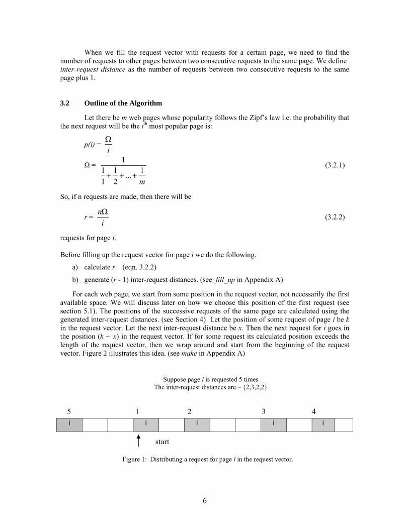
When we fill the request vector with requests for a certain page, we need to find the number of requests to other pages between two consecutive requests to the same page. We define inter-request distance as the number of requests between two consecutive requests to the same page plus 1.

3.2 Outline of the Algorithm

Let there be m web pages whose popularity follows the Zipf’s law i.e. the probability that the next request will be the ith most popular page is:

p(i) = iΩ

Ω =

m1...

21

11

1

+++ (3.2.1)

So, if n requests are made, then there will be

r = i

nΩ (3.2.2)

requests for page i.

Before filling up the request vector for page i we do the following.

a) calculate r (eqn. 3.2.2)

b) generate (r - 1) inter-request distances. (see fill_up in Appendix A)

For each web page, we start from some position in the request vector, not necessarily the first available space. We will discuss later on how we choose this position of the first request (see section 5.1). The positions of the successive requests of the same page are calculated using the generated inter-request distances. (see Section 4) Let the position of some request of page i be k in the request vector. Let the next inter-request distance be x. Then the next request for i goes in the position (k + x) in the request vector. If for some request its calculated position exceeds the length of the request vector, then we wrap around and start from the beginning of the request vector. Figure 2 illustrates this idea. (see make in Appendix A)

Suppose page i is requested 5 times The inter-request distances are – 2,3,2,2

5 1 2 3 4

i i i i i

start

Figure 1: Distributing a request for page i in the request vector.

6

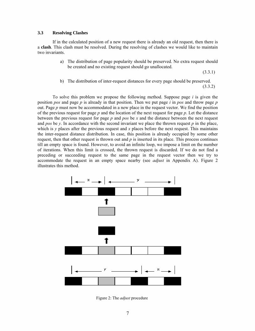
3.3 Resolving Clashes

If in the calculated position of a new request there is already an old request, then there is a clash. This clash must be resolved. During the resolving of clashes we would like to maintain two invariants.

a) The distribution of page popularity should be preserved. No extra request should be created and no existing request should go unallocated. (3.3.1)

b) The distribution of inter-request distances for every page should be preserved. (3.3.2)

To solve this problem we propose the following method. Suppose page i is given the

position pos and page p is already in that position. Then we put page i in pos and throw page p out. Page p must now be accommodated in a new place in the request vector. We find the position of the previous request for page p and the location of the next request for page p. Let the distance between the previous request for page p and pos be x and the distance between the next request and pos be y. In accordance with the second invariant we place the thrown request p in the place, which is y places after the previous request and x places before the next request. This maintains the inter-request distance distribution. In case, this position is already occupied by some other request, then that other request is thrown out and p is inserted in its place. This process continues till an empty space is found. However, to avoid an infinite loop, we impose a limit on the number of iterations. When this limit is crossed, the thrown request is discarded. If we do not find a preceding or succeeding request to the same page in the request vector then we try to accommodate the request in an empty space nearby (see adjust in Appendix A). Figure 2 illustrates this method.

Figure 2: The adjust procedure

7

3.4 Getting the Starting Position

Now we come to the question of how to select the starting position for the requests of a certain web page. We propose two methods. Any one can be chosen depending upon our requirements of speed and accuracy.

In the first method, the starting position of the first web page is generated randomly. The next empty space that comes immediately after the position of the last generated request (not the last request in the request vector) is chosen as the starting position of the next web page. If this position is not empty then we search within a window of size W (defined in section 5.1). In case an empty space cannot be found for the starting position within this window we force it in the next position and the thrown out request is again adjusted using the method adjust (see Appendix A).

In the second method, the starting position of each web page is generated randomly. If there is already another request in that position, then we search for the next empty space in the request vector. 4. Generating the Inter-request Distances

Now we come to the problem of generating inter-request distances for a certain page. We try to generate the distribution of inter-request distances. During the generation step random numbers are picked from this distribution. 4.1 The Inter-request Distance Distribution

For the stack-distance model (see section 2) we assume that the pages are arranged as a push-down stack. If there are m web pages, the size of the stack is m. Consider a given page i. Let the random variable X be the distance of the page i from the top of the stack (stack-distance). If X is equal to 1, then page i is referenced. We model the distribution of X as a Markov chain. Thus these three phrases are synonymous.

1. page i is at the top of the stack

2. page i is requested

3. page i is in state 1 of the Markov chain

From this Markov chain we try to get the probability of page i being requested at time (t+m) given that it requested at time t, with no intervening requests of page i between t and (t+m). This probability is the required inter-request distance probability that we want to generate. This is equal to the first-return-probability defined in section 3. So the problem reduces to finding the sequence of first-return-probabilities of the Markov chain. fii

(1) , fii(2) , ....... fii

(n)

To do so let us construct the transition probability matrix P. Let Xn denote the stack-distance of page i at time n. If Xn=1 page i is at the top of the stack. When the next request is generated, the page i will either remain in state 1 if i is requested again or go to state 2 if any other page is requested.

If Xn=j, 1<j<m then if page i is requested it will go to state 1. If any other page, which is above i in the stack, is requested it will remain in state j. If a page, which is below i in the stack, is requested i will move to state j+1.

If Xn=m, then if the page i is requested it will go to state 1. If any other page is requested, it will remain in state m.

8

Thus the transition probability matrix can be written as

p11 p12 0 0 0 0 . . . . . . . . . . . . . . . . . . . . . . p21 p22 p23 0 0 0 . . . . . . . . . . . . . . . . . . . . . . p31 0 p33 p34 0 0 . . . . . . . . . . . . . . . . . . . . . . p41 0 0 p44 p45 0 . . . . . . . . . . . . . . . . . . . . . .

P = . . . . . . . . . . . . . . . . . . . . . . . . . . . . . . . . . . . . . . . . . . . . . . . . . . . . . . . . . . . . . . . . . . . . . . . . . . . . . . . . . . . . . . . pm-1,1 0 0 0 0 0 . . . . . . . . . . . pm-1,m-1 pm-1,m pm,1 0 0 0 0 0 . . . . . . . . . . . 0 pm,m

We can calculate the transition probabilities as follows.

Let the random variable X denote the stack-distance. The distribution of X is given by the lognormal distribution(lgn(x)). (see section 1.1)

Let gk = Pr(X = k)

We have the following equations :

∑=

m

kkg

1= 1 (4.1.1)

pi,1 = g i = lgn(i) , 1 ≤ i ≤ m (4.1.2)

pi,i = = , 2 ≤ i ≤ m (4.1.3) ∑−

=

1

1

i

kkg ∑

−

=

1

1

)(lgi

k

kn

pi,i+1 = = , 1 ≤ i ≤ m-1 (4.1.4) ∑+=

m

ikkg

1∑

+=

m

ikkn

1)(lg

where lgn(x) represents the lognormal distribution with the parameters given in 1.1.3.

From the transition probability matrix P, we can calculate p11(n) by calculating P(n). Next

we need to calculate the first-return-probabilities from the transition probabilities.

4.2 Methods to Calculate the First-return-probabilities

We designed two methods to calculate first-return-probabilities.

Method I :

Let us define the generating functions.

Pii(s) = n

n

nii sp *

0

)(∑∞

=

Fii(s) = n

n

nii sf *

0

)(∑∞

=

and

9

The relationship between Pii(s) and Fii(s) can be expressed as

Pii(s) = 1

1- Fii(s) or Fii(s) = 1 - 1

Pii(s) (4.2.1)

We know the transition probabilities p11(1), p11

(2), p11(3), … . So we can calculate the

coefficients of Pii(s). We generate a predetermined number of coefficients and then evaluate the values of Pii(s) for different values of s between -1 and +1. This gives us the values of Fii(s) for the corresponding values of s. Then we use simple polynomial interpolation of this sequence to get the coefficients of the generating polynomial Fii(s). This method is fast but it is not very accurate. It was observed that no more than 20 coefficients could be generated. Method II:

Consider the same number of pages m arranged in any order in a push-down stack. We generate the stack-distances using a lognormal distribution (see section 1.1). Using these stack distances, we generate a web page request stream.

Now consider page i. For page i, we can find out the inter-request distances from the request stream. The distribution of these inter-request distances yields the first-return-probabilities (see section 2). So by finding the distribution of the inter-request distances for page i, the first-return-probabilities can be found out.

Thus using either of the above two methods, the first-return-probabilities can be calculated. The question arises: How many values to calculate? 4.3 Calculating the Number of First-return-probabilities

Consider the case of page1, the most popular page. The most popular page has the largest span. The algorithm for allocating requests in the request vector starts at a certain point in the vector and wraps around the end of the vector. The future requests for a certain page should not cross the position of the first request allocated for that page. Otherwise, the inter request distances will violate invariant 3.3.2. We derive a relation to ensure that this property is achieved. Let z be the mean inter-request distance calculated by just considering the fact that page popularity follows the Zipf distribution (section 1.1). Let l be the mean inter-request distance calculated by the Markov chain model (section 4.2). Let the total number of requests generated be n.

Number of requests for page 1 from the Zipf model is : zn

(4.3.1)

Number of requests for page 1 from the analysis in 4.2 : ln

(4.3.2)

If both the model for page popularity and temporal locality are to be followed then there must be an equality of (4.3.1) and (4.3.2). This equality also ensures that the most popular page is distributed uniformly in the request stream.

Thus,

z = l (4.3.3)

We can calculate z as follows:

10

The probability of occurrence of page 1 is 1Ω

= Ω. Thus the number of requests to page 1 is nΩ.

Thus

Ω=⇒

Ω=

1z

nzn

(4.3.4)

If the number of first return probabilities considered is d then l is given by :

∑=

=d

i

ifil1

)(11* (4.3.5)

So if (4.3.3) is to hold then:

∑=

=Ω

d

i

ifi1

)(11*1

(4.3.6)

By (3.2.1)

∑=

=+++d

i

ifim 1

)(11*1.....

21

11

(4.3.7)

Thus, given the number of pages m, we can calculate the number of coefficients required, d. A plot of log(d) versus log(m) is shown.

Figure 3: log-log plot of number of coefficients vs. number of pages

11

We find this graph to be approximately linear. From the above graph, we find the relation between m and d as

log(d) = 0.24*log(m) + 0.86 (4.3.8)

Thus we can use (4.3.8) to calculate the number of coefficients required given the number of web pages.

Hence using the methods of (4.2) and the result of (4.3.8) we can generate the inter-request distance distribution. To generate inter-request distances we just pick random numbers from this distribution (see get_rand() in Appendix A). 5. Salient Features of the Algorithm

In this section we analyze some features of the algorithm presented in section 3. We allude to the pseudo code in Appendix A. Some design decisions have been taken that bound the worst case complexity and significantly decrease the running time and improve the quality of output. Sections 5.1 and 5.2 discuss the schemes for filling up page requests. While filling up these pages it is sometimes necessary to search for an empty slot or to adjust the requests in the request vector. We derive bounds for the number of iterations in these procedures in sections 5.3 and 5.4. Sections 5.5 and 5.6 discuss the quality of the output and section 5.7 concludes with the complexity measures.

NOTE: The term ‘first request of a page’ means the first request of a page allocated in the request vector by our algorithm. It should not be confused with the first request of a page in the request stream. We might starting allocating page i from the 990th request in a stream of 1000 requests. Then we might wrap around and allocate pages 1, 50, 100. The ‘first request of page i’ is 990 and the ‘first request of page i in the request stream’ is 1. 5.1 Position of the First Request of a Page

We have presented two solutions. The first solution remembers the position of the last request of the last page allotted. For the first request of the present page it searches W positions after the last request for an empty space. If an empty space is found then the first request for the present page is inserted in that space and the normal algorithm continues. If an empty space is not found then at the (W + 1) th position after the last request, the present page is inserted and adjust is called. It is to be noted that whenever a position exceeds the number of requests it wraps around and starts from the beginning.

For the second solution we start at a random position while allotting the first request of a page. If this position is empty then we insert the page. If it is not then we search for the nearest empty slot.

After the algorithm terminates, some slots in the request vector might remain unfilled. This is because we have placed a limit on the number of iterations in adjust (see section 5.3). The goal is to minimize the number of unfilled positions after the algorithm ends. So we perform a linear search for the first request of a page instead of calling adjust. This was found to reduce the number of unfilled positions in the request vector. Note that by the Zipf distribution the last few pages will occur only once. By the time they are allocated the request vector is almost full. So the number of clashes will be very high. It is easier to do a linear search and find an empty slot.

12

There are tremendous performance advantages in the first approach. This is because the region of the request vector in which the requests for a certain page are being filled up is the least congested part of the request vector. Thus clashes are always at a minimum. Because of this property we can provide an upper bound on the constant W defined earlier. A good estimate of W is 3*d (4.3.8). Most of the time we find an empty space within this window size. Since we bound W by a constant the asymptotic complexity becomes O(nm0.24) (see Appendix B). This approach ensures a certain amount of spatial locality. However, in this approach we sacrifice a bit of uniformity and randomness in request streams.

The second approach is far slower. The property of least congestion observed in the first approach is not valid here as the first requests to be allocated for any page start at random positions. This necessitates searching the full request vector for an empty space while allocating the first request of a page, making the asymptotic complexity O(nm) (see Appendix B). Although, this is far slower than the previous algorithm it shows uniformity and randomness in requests. 5.2 The Order of Filling up of Pages

We always start filling up the request vector with pages in descending order of popularity. Popular pages have bigger spans. Span refers to the distance between the first and last request of the same page. Less popular pages don’t feel the effects of congestion due to allocation of other less popular pages due to their small spans. However, more popular pages with bigger spans are distributed globally and feel the effects of all other pages allocated before them. Experimental results have shown an improvement in speed of a factor of 7 for this scheme compared to the scheme where page requests are allocated in ascending order of popularity of pages. 5.3 Limit on the Number of Iterations in adjust

It was experimentally observed that the average number of iterations in the method adjust was about 8.5. This was independent of the number of pages and requests. So, we set the limit on the number of iterations to a safe constant 100. This is a constant irrespective of the input parameters. 5.4 Limit on the Number of Iterations in get_new_position

In the procedure get_new_position the preceding and succeeding requests of a web page are found out. It is to be noted that the maximum inter-request distance is d (4.3.8). So there is no need to search positions, which have a distance greater than d from the present position.

5.5 Loss Percentage

The loss percentage is the number of slots in the request vector that could not be allocated. Some loss is incurred due to a limit on the number of iterations in adjust. The number of unfilled slots is typically less than 1% of the number of requests. 5.6 Increase in Accuracy with Increase in Number of Pages

As the number of pages increase the number of coefficients of the first-return-probability distribution also increase (4.3.8). Thus the inter-request distance distribution becomes more accurate. Hence, it follows from section 4.1 that the final stack-distance distribution also becomes more accurate.

13

5.7 Complexity of the Algorithm

The complexity is analyzed in Appendix B. The fast version of the algorithm runs in O(n*m0.24) time. This is suitable for simulation purposes. It runs in linear time in the number of requests. This algorithm has a very fast running time owing to the fact that m0.24 is a slowly growing function.

The slow version runs in O(nm) time. This generates high quality request streams. High-speed machines are required to execute this algorithm or alternatively workstations can be used to generate traces that can be used later for simulation.

6. Results We executed the fast version of the algorithm for different combinations of requests and

pages. As a rule of thumb we assumed the number of requests to be ten times the number of pages. The experiments were conducted on a 866Mhz, 256MB RAM, Pentium III machine running RedHat Linux 7.1. The following table shows the execution times of the various experiments conducted.

Number of Pages ( m ) Number of requests ( n ) Execution time (sec) 3,000 30,000 0.02

10,000 100,000 0.08 20,000 200,000 0.17 50,000 500,000 0.48

100,000 1,000,000 1.03

As we can see, the complexity of the algorithm is almost linear in the number of requests.

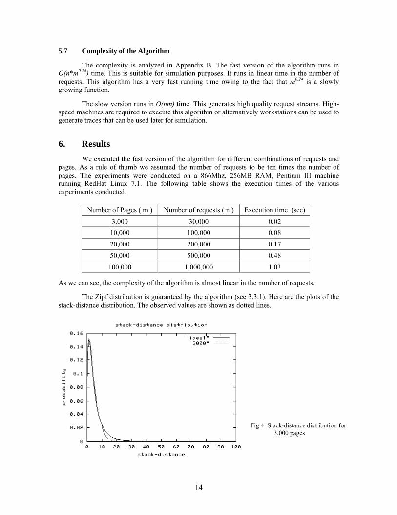
The Zipf distribution is guaranteed by the algorithm (see 3.3.1). Here are the plots of the stack-distance distribution. The observed values are shown as dotted lines.

Fig 4: Stack-distance distribution for 3,000 pages

14

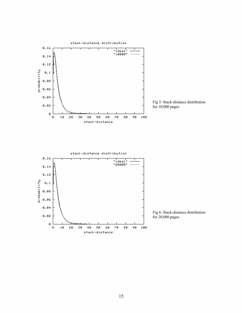
Fig 5: Stack-distance distribution for 10,000 pages

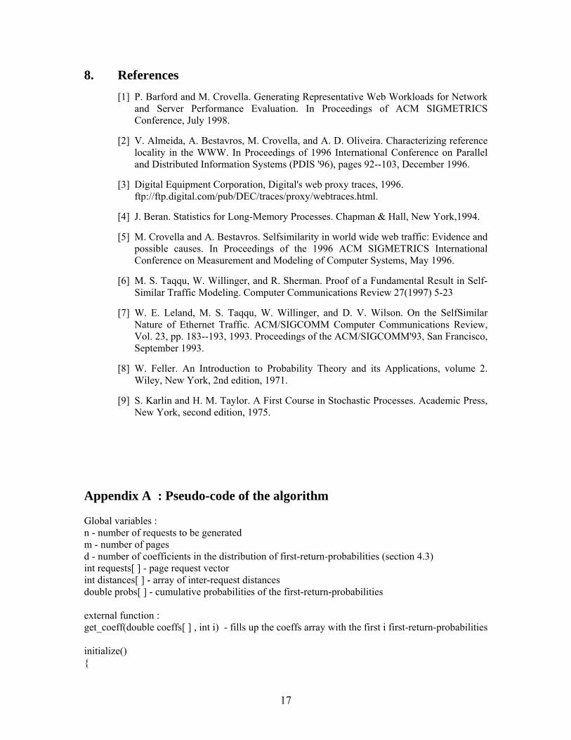
Fig 6: Stack-distance distribution for 20,000 pages

15

Fig 7: Stack-distance distribution for 50,000 pages

7. Conclusion

In this paper we have presented an algorithm to generate high quality web request streams. The work is based on analytical models derived from measurements of web traffic. The major characteristics of web request streams have been incorporated into our method. The properties of the traces generated are shown to follow the empirically observed distributions of page popularity and temporal locality. The algorithm guarantees the Zipf distribution of page popularity and the results show the stack-distance distribution to mimic very closely the ideal lognormal distribution very closely. We have two versions of the algorithm presented in this paper. One is the fast algorithm whose worst-case complexity is linear in the number of requests and is a slowly growing function of the number of pages. This algorithm explicitly incorporates spatial locality into the request stream. The other version is the slow algorithm, whose complexity is linear in the number of request and linear in the number of pages. This generates uniform and homogenous request streams.

Along with the quality of traces the algorithm is also computationally efficient and scalable. The quality is maintained even for a large number of pages and requests. In fact the quality of the traces improves with increase in the number of pages.

As indicated in section 1.1 spatial locality needs to be incorporated into the algorithm. Even though the fast version of the algorithm guarantees some spatial locality, it does not strictly conform to analytical models of spatial locality. Self-similar models of stack distance need to be explicitly incorporated.

To summarize, the algorithm presented in this paper generates request streams in accordance with analytical models of web traffic. It is scalable to a large number of requests and it requires minimal amount of memory and processor time. The accuracy, scalability and computational efficiency of our algorithm attest its suitability for large-scale WAN simulation.

16

8. References [1] P. Barford and M. Crovella. Generating Representative Web Workloads for Network

and Server Performance Evaluation. In Proceedings of ACM SIGMETRICS Conference, July 1998.

[2] V. Almeida, A. Bestavros, M. Crovella, and A. D. Oliveira. Characterizing reference locality in the WWW. In Proceedings of 1996 International Conference on Parallel and Distributed Information Systems (PDIS '96), pages 92--103, December 1996.

[3] Digital Equipment Corporation, Digital's web proxy traces, 1996. ftp://ftp.digital.com/pub/DEC/traces/proxy/webtraces.html.

[4] J. Beran. Statistics for Long-Memory Processes. Chapman & Hall, New York,1994.

[5] M. Crovella and A. Bestavros. Selfsimilarity in world wide web traffic: Evidence and possible causes. In Proceedings of the 1996 ACM SIGMETRICS International Conference on Measurement and Modeling of Computer Systems, May 1996.

[6] M. S. Taqqu, W. Willinger, and R. Sherman. Proof of a Fundamental Result in Self-Similar Traffic Modeling. Computer Communications Review 27(1997) 5-23

[7] W. E. Leland, M. S. Taqqu, W. Willinger, and D. V. Wilson. On the SelfSimilar Nature of Ethernet Traffic. ACM/SIGCOMM Computer Communications Review, Vol. 23, pp. 183--193, 1993. Proceedings of the ACM/SIGCOMM'93, San Francisco, September 1993.

[8] W. Feller. An Introduction to Probability Theory and its Applications, volume 2. Wiley, New York, 2nd edition, 1971.

[9] S. Karlin and H. M. Taylor. A First Course in Stochastic Processes. Academic Press, New York, second edition, 1975.

Appendix A : Pseudo-code of the algorithm Global variables : n - number of requests to be generated m - number of pages d - number of coefficients in the distribution of first-return-probabilities (section 4.3) int requests[ ] - page request vector int distances[ ] - array of inter-request distances double probs[ ] - cumulative probabilities of the first-return-probabilities external function : get_coeff(double coeffs[ ] , int i) - fills up the coeffs array with the first i first-return-probabilities initialize()

17

for i ← 0 to (n-1) loop distances[ i ] ← 0 requests[ i ] ← -1

end loop

double coeff[d ] get_coeff( coeff, d) probs[ 0 ] ← 0.0

for l ← 1 to size loop

probs[ l ] = coeff [l-1] end loop

for j ← 1 to size loop

probs[ j ] += probs[ j-1] end loop

// generates the request vector generate (distances[ ], requests[ ]) 1 for i ← 1 to m loop 2 fill_up ( i, distances ) 3 make ( i, requests, distances ) 4 end loop // fills up the distance array with the inter-request distances fill_up (page, distances[ ]) // calculate the number of inter-request distances 1 spaces = num_occur(i) - 1 // fill up the distances array 2 for i ← 1 to (spaces – 1) loop 3 distances[ i ] = get_rand( i ) 4 end loop // fills up the request vector // starting position is selected using the faster method make (page, requests[ ], distances[ ]) 1 static int pos = rand() % n

// finds the first free position within the window of 3*d

2 for i ← 1 to (3 x d) loop 3 if ( free(request[pos] ) 4 flag ← 1

18

5 break 6 end if 7 pos++ 8 if ( pos = n ) pos ← 0 // wrapping around 9 end loop 10 if ( !flag ) adjust ( pos, page, requests ) // if no empy space is found 11 else requests[ pos ] ← page 12 spaces ← num_occur(page) – 1 13 if (spaces = 0) return // there is just one request // filling up the rest of the requests 14 for j ← 0 to (spaces – 1) loop 15 pos ← pos + distances[ j ] // finding the position of the next request 16 if (pos ≥ n ) pos ← pos % n // wrapping around 17 if ( free (requests[ pos ] ) requests[ pos ] ← page 18 else adjust( pos, page, requests) 19 end loop // permutes the request vector in accordance with the invariants ( 3.3.1 and 3.3.2 ) const LIMIT ← 100 // (see section 5.2 ) adjust (pos, page, requests[ ] ) 1 limit ← 0 2 thrown ← requests[ pos ] 3 requests [ pos ] ← page 4 while (thrown != -1 ) 5 i ← get_new_position(pos, thrown, requests) 6 swap( requests[ i ], thrown) 7 if (limit = LIMIT ) return 8 limit++ 9 end while // gets a new position for a request in accordance with the invariants ( 3.3.1 and 3.3.2 ) int get_new_position (pos, page, requests[ ]) // find the preceding request for the same page 1 lower ← -1 2 for i ← (pos – 1) to max(0, pos – m ) loop 3 if ( free(requests[ i ] ) 4 lower ← i 5 break

19

6 end if 7 end loop // find the succeeding request for the same page 8 upper ← -1 9 for j ← (pos+1) to min(n-1, pos+m) loop 10 if (free(requests[ i ] ) 11 upper ← i 12 break 13 end if 14 end loop // if upper or lower don’t exist 15 if ( (lower = -1) or (upper = -1) ) 16 for k ← max(0, pos-3) to min (n-1, pos+3) loop 17 if (k=pos) continue 18 If (free(requests[ k ]) return k 19 end loop 20 if (pos < (n-2) ) return (pos+2) 21 else return (pos – 2) 22 end if // calculate the new position based on invariant (3.3.2) 23 x ← lower + upper – pos // handling special cases 24 If (x = pos) pos++ 25 If (pos = upper) pos = (pos+1)%n 26 return pos // finds the number of requests for page i int num_occur( int i )

val ← iΩ

return ( val x n ) // generates a random number following the distribution of first-return-probabilities (see section 4.2) int get_rand() 1 val ← frand() // returns a random number between 0 and 1 2 i ← binary_search(probs, val) 3 return i

20

Another make method used in the slow algorithm, where the starting position is selected using the second method. (see section 3.4) make (page, requests[ ], distances[ ])

// position of the first request of a page 1 pos ← rand() % n

// find the next free slot

2 for i ← 1 to n loop 3 if (free(request[i]) 4 flag ← 1 5 break 6 end if 7 if (pos = n) pos ← 0 // wrap around 8 end loop 9 if (!flag return) // no empty space found 10 requests[pos] = page 11 if (spaces = 0) return // this page just had 1 request 12 for j ← 0 to (spaces – 1) loop 13 pos ← pos + distances[ j ] 14 if (pos ≥ n ) pos ← pos % n // wrap around 15 if ( free (requests[ pos ] ) requests[ pos ] ← page 16 else adjust( pos, page, requests) 17 end loop Appendix B : Complexity of the algorithm The parameters of the algorithm are :

• n - number of requests • m - number of pages • d - number of first return probabilities (see section 4.3)

By equation 4.38 : O(log(m)) ↔ O(log(d)) Let fi be the number of requests for page i.

∑ =i

i nf

1. The complexity of the fast algorithm. This uses the first make method.

21

function complexity explanation

get_rand() O(log(m)) (2) takes O(log(d)) time. Hence, the function takes O(log(m)) time.

num_occur() O(1) There are no loops or function calls.

fill_up(i , array[ ]) O(fi * log(m)) (3) is executed fi times.

get_new_position(i, j, array[ ])

O(m0.24)) (2) - (7) takes O(d) time (9) - (14) takes O(d) time

rest takes O(1) time O(d) ↔ O(m0.24) (eqn 4.3.8)

adjust(i, ,j, array [ ]) O(m0.24) (5) is executed at most LIMIT times

make(i, array1[ ] , array2[ ])

O(fi * m0.24) (2) - (9) takes O(d) time (10) takes O(d) time

(18) is executed O(fi) times. (14) - (19) takes O(fi * d) time

O(fi * d) ↔ O(fi * m0.24) generate(array1[ ],

array2[ ]) O(n * m0.24) (2) - (3) takes O(fi * (m0.24 + log(m))) ↔ O(fi *

m0.24) time (1) - (4) takes O((∑

iif ) * m0.24 ) ≡

O(n * m 0.24) time

2. The complexity of the slow algorithm. This uses the second make method

function Complexity explanation

make(i, array1[ ] , array2[ ])

O(n + fi * m0.24) (2) - (8) takes O(n) time (16) takes O(d) ↔ O(m0.24) time

(12) - (17) takes O(fi * m0.24) time

generate(array1[ ], array2[ ])

O(nm) (2) - (3) takes O(n + fi * (m0.24 + log(m))) ↔ O(n + fi * m0.24) time

(1) - (4) takes O(nm + (∑i

if ) * m0.24) ↔

O(nm + n * m0.24) ↔ O(nm) time

22