Generating VPL Expressions

Visual Expression(e.g. Graphs)

a

+b

c := a + b;...

Abstract Data(e.g. program)

Implementing a Visual Language (often) requires transformation between visual expressions and abstract data.

- Converting visual expressions into abstract data can either be done incrementally (event-based) or with parsing-based methods

- Converting abstract data into visual expressions requires automatic layout techniques

parsing

layoutc

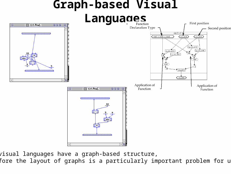
Graph-based Visual Languages

Most visual languages have a graph-based structure, therefore the layout of graphs is a particularly important problem for us.

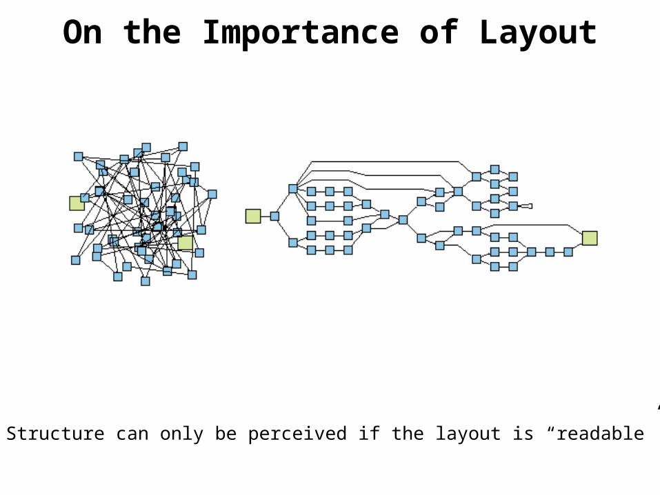
On the Importance of Layout

Structure can only be perceived if the layout is “readable”

Project

In the project assignment you will have to implement a “layout tool” that performs automatic layout of graphs, i.e. of the type of visual expressions that are used in Prograph and related VPLs, in particular DFPLs. This can, in principle,be compared to pretty-printing Prograph-programs.

Your program will not have to layout Prograph expressions directly, but will onlyimplement such a layout in “principle”.

You will have to write a small graph editor that allows to draw simple graphswhich can then be layed out (i.e. “re-drawn nicely”) by the program automatically, i.e. without further user intervention.

Simple graphs means that all nodes are idealized.(rectangles or circles of a constant size) and so are all edges (lines of constant thickness).

A precise specification of the project will be given to you in the next lecture.

Graph Drawing Applications

Graph or network-like structures are among the most commonly usedtypes of visual representations. Therefore the automatic layout of graphs plays an important role in many applications:

- Visual Programming - Software Engineering

(e.g. Flow-Charts, UML, Dependency visualization, Repository Structures)

- Engineering(e.g. Circuit Diagrams, Molecular Structures, Chemical Formulas)

- Sciences(e.g. Genome Diagrams...)

- currently a particularly hot-topic: Web-Visualization

Almost always when relational data that has been obtained as the result of anautomated operation such as a database or repository computation, a web-crawl or another kind of computation) has to be visualized, we are faced with the problem of automatic graph layout.

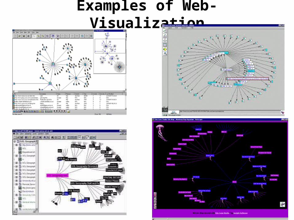
Examples of Web-Visualization

taken from the Atlas of Cyberspaces (http://www.cybergeograph.org)

Examples of Web-Visualization

Examples of Web-Visualization

Intranet Visualization

Graph Drawing as a Research Field

Automatic layout of graphs is a very complex and mathematically challengingproblem. It has therefore spawned a whole field of research with its ownconference series: The International Symposium on Graph Drawing (since 1992)

Proceedings are published in Springer-Verlag’s “Lecturer Notes in Computer Science series”

The best (and only comprehensive) book on the topic is:Graph Drawing by G. DiBattista, P. Eades, R. Tamassia and I.G. Tollis,Prentice Hall, 1999.

All references in these notes are listed in this book’s bibliography.

One of the authors also maintains a very good web page on this topic:http://www.cs.brown.edu/people/rt/gd.html

From here you can also reach the pages for the symposium.

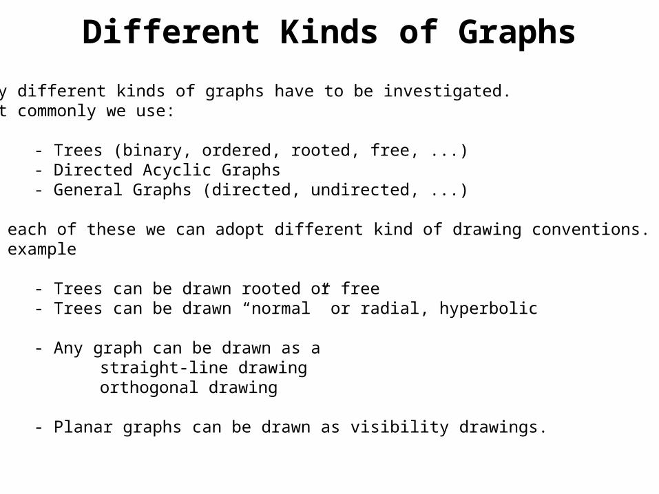
Different Kinds of Graphs

Many different kinds of graphs have to be investigated.Most commonly we use:

- Trees (binary, ordered, rooted, free, ...)- Directed Acyclic Graphs- General Graphs (directed, undirected, ...)

For each of these we can adopt different kind of drawing conventions.For example

- Trees can be drawn rooted or free- Trees can be drawn “normal” or radial, hyperbolic

- Any graph can be drawn as a straight-line drawing orthogonal drawing

- Planar graphs can be drawn as visibility drawings.

Orthogonal Drawings

visibility drawing

orthogonal drawing

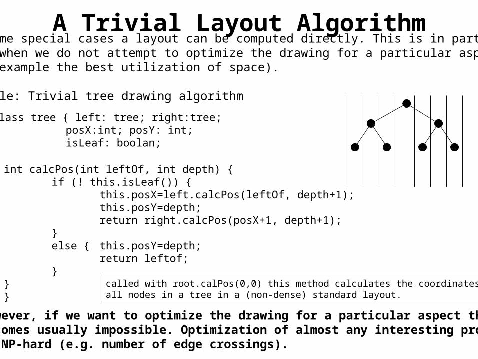
A Trivial Layout Algorithmin some special cases a layout can be computed directly. This is in particulartrue when we do not attempt to optimize the drawing for a particular aspect(for example the best utilization of space).

Example: Trivial tree drawing algorithm

int calcPos(int leftOf, int depth) {if (! this.isLeaf()) {

this.posX=left.calcPos(leftOf, depth+1);this.posY=depth;return right.calcPos(posX+1, depth+1);

}else { this.posY=depth;

return leftof;}

}}

class tree { left: tree; right:tree; posX:int; posY: int; isLeaf: boolan;

called with root.calPos(0,0) this method calculates the coordinates forall nodes in a tree in a (non-dense) standard layout.

However, if we want to optimize the drawing for a particular aspect this becomes usually impossible. Optimization of almost any interesting propertyis NP-hard (e.g. number of edge crossings).

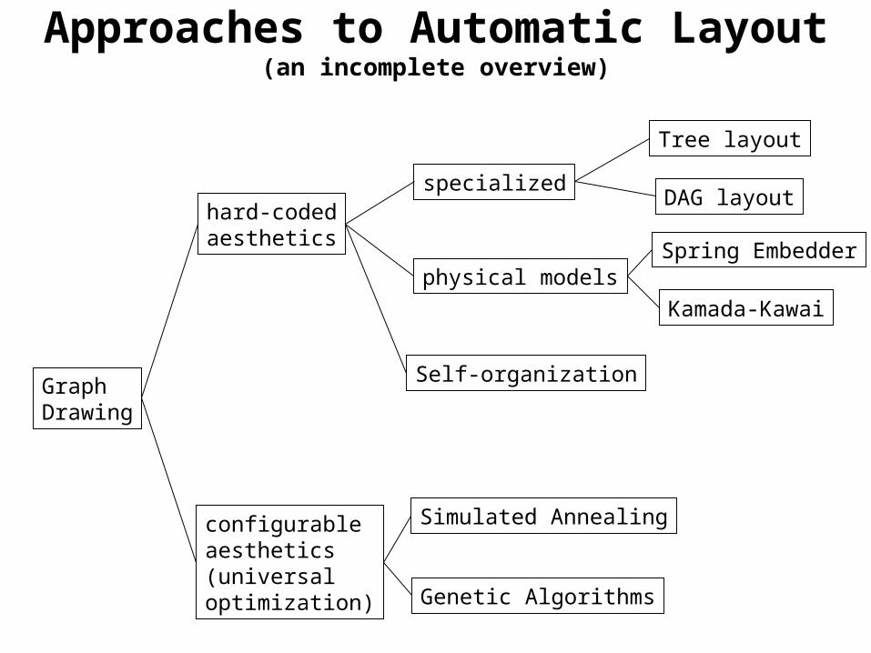
Graph Drawing Aesthetics

However, in most cases automatic graph layout is not as easy.One of the reasons is that we are mostly faced with graphs in which wecannot identify an implicit node order (general graphs).

The most important problem is that, in general, we want to optimize the drawing for comprehensibility and aesthetics. This implies an optimization problem which is hard to solve.

Of course, we need to formalize what these criteria mean (mathematically).The most commonly used aesthetic criteria are: - expose symmetries- make drawing compact / fill available space

- minimized number of edge crossings- evenly distributed edge length- evenly distributed node positions- sufficiently large node-edge distances- sufficiently large angular resolution

Graph Drawing as Optimization

The aesthetic objective function takes node positions as input and returns a numerical measurement of its “beauty”.

f(g) = c1 * #crossings(g) +c2 * 1/std-deviation-edge-length(g) +...

This turns graph layout into a general optimization problem

Most of the sub-problems, e.g. the mimimizationof edge-crossings are already known to be NP-hard.

A straight-forward full optimization is often not feasible.

Usually stochastic / heuristic methods are employed.

Approaches to Automatic Layout(an incomplete overview)

GraphDrawing

specialized

Tree layout

DAG layouthard-codedaesthetics

physical models

configurableaesthetics(universaloptimization) Genetic Algorithms

Simulated Annealing

Spring Embedder

Kamada-Kawai

Self-organization

Spring Embedder Layout (Idea)

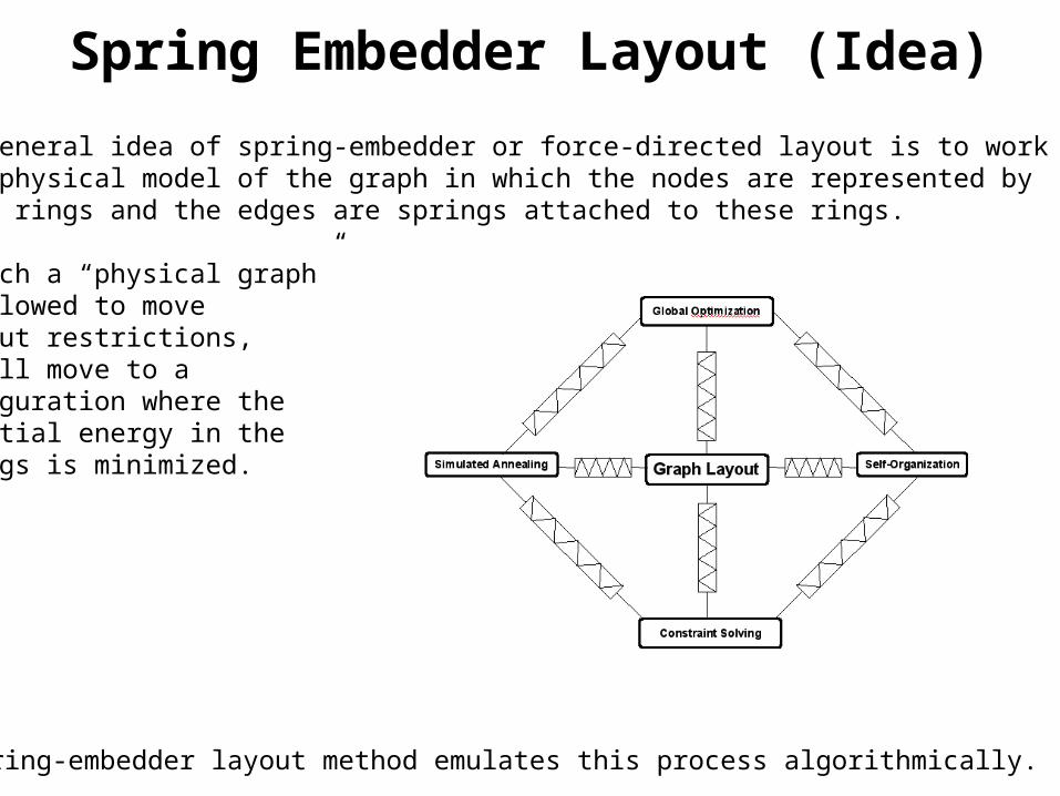
The general idea of spring-embedder or force-directed layout is to workon a physical model of the graph in which the nodes are represented by steel rings and the edges are springs attached to these rings.

If such a “physical graph” is allowed to move without restrictions, it will move to a configuration where the potential energy in the springs is minimized.

A spring-embedder layout method emulates this process algorithmically.

Energy AnalysisAccording to Hooke’s law (spring law), the spring force is approximated by

Fs

=−ks

len−len0( ) =−kΔlen

where len0 is the natural length of the (resting) spring.

We also add a second, repulsive force, which is used to achieve even node distribution. This force is modelled as an analogy to electrical forces.

Fe

=ke

d2We also add a second, repulsive force, which is used to achieve even node distribution. This force is modelled as an analogy to electrical forces.

Attractive forces are only considered between incident nodes, repulsive forcesbetween all nodes. Thus the total force acting at a node is:

F = ks(d(u,v)−l)

(u,v)∈E∑ +

ke

d(u,v)2(u,v) ∈V×V∑

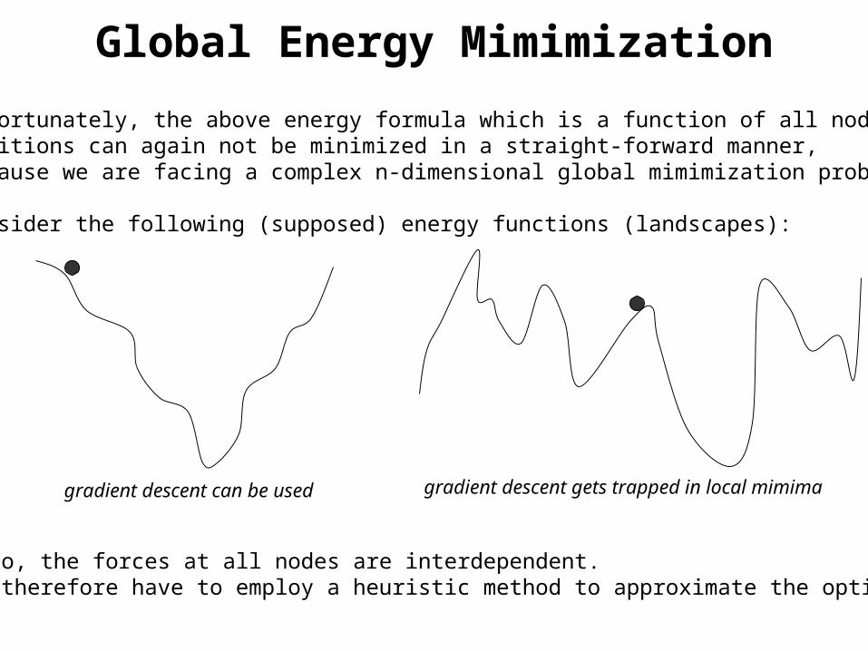
Global Energy Mimimization

Unfortunately, the above energy formula which is a function of all node positions can again not be minimized in a straight-forward manner, because we are facing a complex n-dimensional global mimimization problem:

Consider the following (supposed) energy functions (landscapes):

Also, the forces at all nodes are interdependent.We therefore have to employ a heuristic method to approximate the optimum.

gradient descent can be used gradient descent gets trapped in local mimima

Fruchterman-Rheingold (Idea)Fruchterman and Rheingold [FR91] have defined as simple heuristic approachto force-directed layout that works surprisingly well in practice.

The basic idea is to just calculate the attractive and repulsive forces at eachnode independently and to update all nodes iteratively.

The forces take a somewhat different form (justified by experimentation).The attractive force is:

Additionally, the maximum displacement of each node in an iteration is limitedby a constant that is slightly decreased with each iteration.

where k is chosen as

and the repulsive force is:

fa(x) =

x2

k

fr(x) =

k2

x

k=areaV

A very compact description is given in: “Simulating Graphs as Physical Systems”, A. Frick, G. Sander and K. Wang in Dr. Dobbs Journal, August 1999.

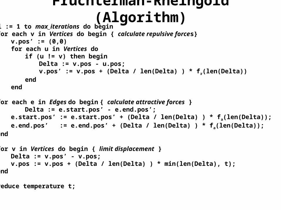
Fruchterman-Rheingold (Algorithm)

for i := 1 to max_iterations do beginfor each v in Vertices do begin { calculate repulsive forces}

v.pos’ := (0,0)for each u in Vertices do

if (u != v) then beginDelta := v.pos - u.pos;v.pos’ := v.pos + (Delta / len(Delta) ) * fr(len(Delta))

endend

for each e in Edges do begin { calculate attractive forces }Delta := e.start.pos’ - e.end.pos’;

e.start.pos’ := e.start.pos’ + (Delta / len(Delta) ) * fa(len(Delta));e.end.pos’ := e.end.pos’ + (Delta / len(Delta) ) * fa(len(Delta));

end

for v in Vertices do begin { limit displacement }Delta := v.pos’ - v.pos;v.pos := v.pos + (Delta / len(Delta) ) * min(len(Delta), t);

end

reduce temperature t;

end

Fruchterman-Rheingold (Examples)

Evaluation of Force-Directed Layout

Force-directed Layout is quite useful, because it is a good class of heuristicmethods that find nice layouts of general graphs.

These drawings even automatically expose (most of the) symmetries of thegiven graphs.

However, a number of problems remain:

- These methods are still computationally expensive- There is no guarantee for a true optimization.- It is difficult to integrate additional constraints

(such as preferred node orders, alignments etc.)- Often edge crossings remain, even in planar graphs- They treat only idealized graphs,

node extensions and shapes, label positions etc. are not taken into account

- Still, force-directed methods are among the most popular approaches anda large number of variants (with additional forces) have been explored.

GD as Global Optimization

both of the above graph layout schemata, though in practicevery useful are relatively limited, because they follow a fixed “physical” model.Their aesthetic criteria are hard-wired and can only be changed to a limited degree by introducing new forces (e.g. radial forces, orthogonal forces etc.)

As outlined above, we can also use a general optimization method to performgraph-drawing. The idea is to define an objective function which formalizes the “aesthetic value” of the graph.

Let G be the set of all graphs, R the set of real number. We define an objective function

A universal mathematical optimization method can then be used to find theplacement of nodes that minimizes the objective function f.

f: G -> R,f(g) = c1 * number-of-crossings(g) +

c2 * 1/std-deviation-edge-length(g) +...

Objective Function Composition

the most popular of these approaches has been presented in:

R. Davidson and D. Harel. Drawing Graphs Nicely Using Simulated Annealing.ACM Transactions on Graphics, 15(4):301-331, October 1996.

Here the objective functions has (based on extensive experiments) been chosen as follows:

f(g) = λ1⋅ 1

d(ni,n

j)

i ≠ j∑ Nodedistribution

+λ2

⋅ dborder

(ni)

i∑ Borderlinedistance

+λ3

⋅ d(ni,n

j)

(ni,n

j) ∈V

∑ EdgeLength

+λ4

⋅num(crossings) EdgeCrossings

+λ5

⋅ d(ni,e

i, j)

(ni,n

j)∈V

∑i∑ Edge−Edgedistance

Reminder Local versus Global MimimizationTo find the global mimimum of this function, it is not sufficient to perform a local search with a gradient descent procedure (hill climbing), since the objective function can have multiple local minima.

Consider the following functions:

gradient descent can be used gradient descent gets trapped in local mimima

Gradient Descent

Assume we want to mimimize f(x) for a simple function of a single variable:f: R -> R.

A local search by gradient-descent (hill climbing) works in the following manner:

initialize x = starting-point;initialize y = f(x);improved = true;

while improved do set x’ to a neighbouring value of x;if f(x’) < f(x) do

x = x’; else

improved = false;end

end.

In other words, the method modifies x slightly locallyas long as the objective value improves.

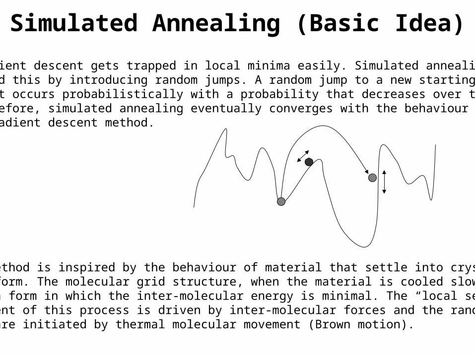
Simulated Annealing (Basic Idea)

Gradient descent gets trapped in local minima easily. Simulated annealing avoid this by introducing random jumps. A random jump to a new starting point occurs probabilistically with a probability that decreases over time.Therefore, simulated annealing eventually converges with the behaviour of a gradient descent method.

This method is inspired by the behaviour of material that settle into crystallinesolid form. The molecular grid structure, when the material is cooled slowlytakes a form in which the inter-molecular energy is minimal. The “local search” component of this process is driven by inter-molecular forces and the randomjumps are initiated by thermal molecular movement (Brown motion).

Simulated Annealing (Basic Algorithm)

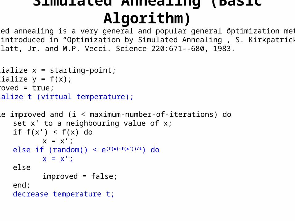
Simulated annealing is a very general and popular general optimization method.It was introduced in “Optimization by Simulated Annealing”, S. Kirkpatrick and C.D. Gelatt, Jr. and M.P. Vecci. Science 220:671--680, 1983.

initialize x = starting-point; initialize y = f(x); improved = true;intialize t (virtual temperature);

while improved and (i < maximum-number-of-iterations) do set x’ to a neighbouring value of x;if f(x’) < f(x) do

x = x’; else if (random() < e(f(x)-f(x’))/t) do

x = x’;else

improved = false;end;decrease temperature t;

end.

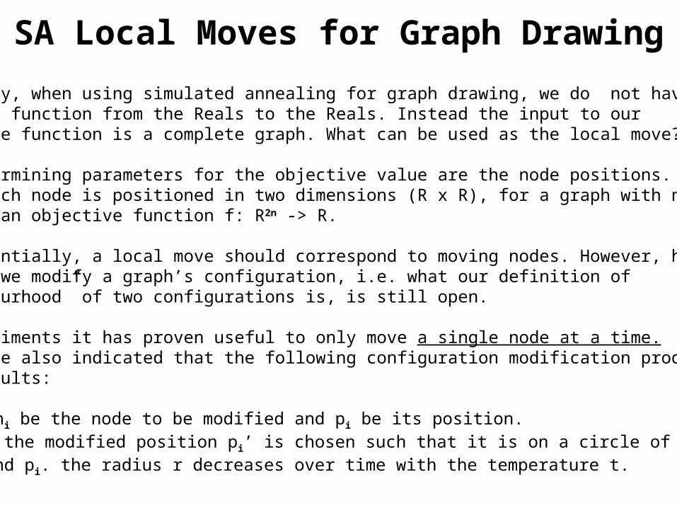
SA Local Moves for Graph Drawing

Obviously, when using simulated annealing for graph drawing, we do not havea simple function from the Reals to the Reals. Instead the input to our objective function is a complete graph. What can be used as the local move?

The determining parameters for the objective value are the node positions.Since each node is positioned in two dimensions (R x R), for a graph with n nodeswe have an objective function f: R2n -> R.

Consequentially, a local move should correspond to moving nodes. However, howexactly we modify a graph’s configuration, i.e. what our definition of “neighbourhood” of two configurations is, is still open.

In experiments it has proven useful to only move a single node at a time.They have also indicated that the following configuration modification producesgood results:

Let ni be the node to be modified and pi be its position. Then the modified position pi’ is chosen such that it is on a circle of radius r around pi. the radius r decreases over time with the temperature t.

SA Example Animation

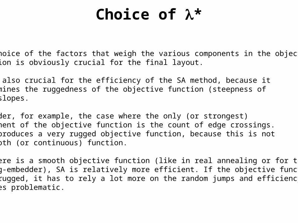
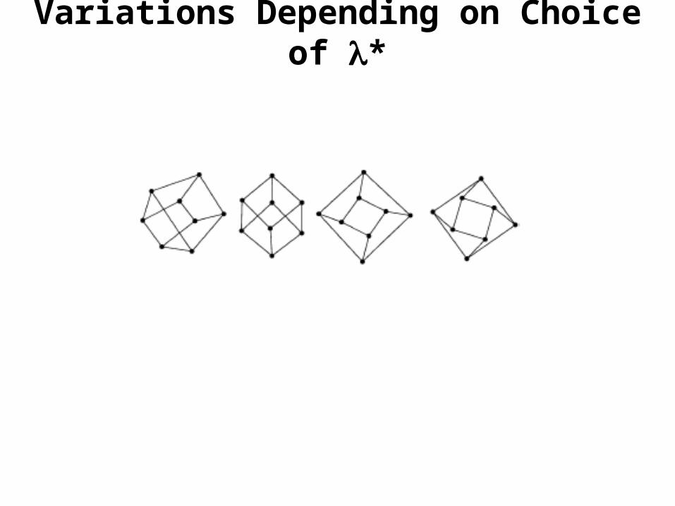
Choice of *

The choice of the factors that weigh the various components in the objective function is obviously crucial for the final layout.

It is also crucial for the efficiency of the SA method, because it determines the ruggedness of the objective function (steepness of its) slopes.

Consider, for example, the case where the only (or strongest)component of the objective function is the count of edge crossings.This produces a very rugged objective function, because this is nota smooth (or continuous) function.

If there is a smooth objective function (like in real annealing or for the spring-embedder), SA is relatively more efficient. If the objective function is very rugged, it has to rely a lot more on the random jumps and efficiencybecomes problematic.

Variations Depending on Choice of *

More SA-GD Examples

Summary Simulated Annealing for GD

is expensive, but theoretically guaranteed to find the global mimumum.

However, in practice this guarantee is not valid, since it requiresa potentially infinite runtime.

In practice, to reach sufficiently fast convergence a considerable amount of fine tuning is required regarding

•objective function•configuration neighbourhood•termination criteria

•cooling schedule (temperature as a function of time).

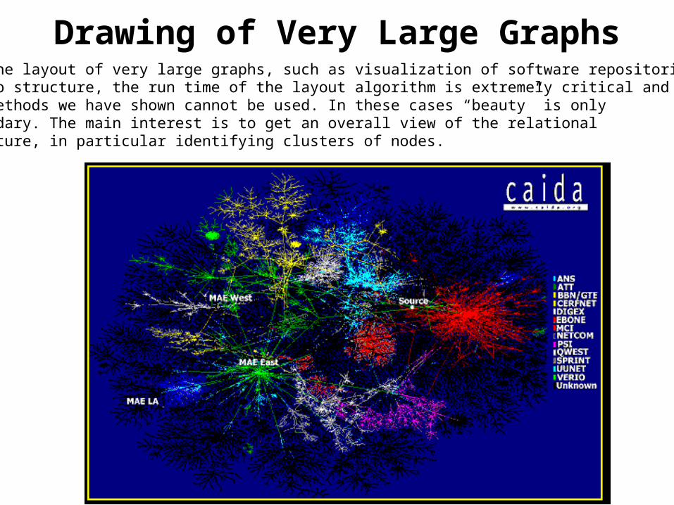
Drawing of Very Large GraphsFor the layout of very large graphs, such as visualization of software repositoriesor web structure, the run time of the layout algorithm is extremely critical andthe methods we have shown cannot be used. In these cases “beauty” is onlysecondary. The main interest is to get an overall view of the relational structure, in particular identifying clusters of nodes.

Fast Layout Methods for Large Graphs

For the drawing of very large graphs much faster clustering algorithms must be used and a finer and more detailed layout may be generated after obtaining a smaller graph by zooming in (and/or removing irrelevant nodes).

For examples of such algorithms see:

Self-organizing Graphs.B. Meyer. In International Symposium on Graph Drawing 1998. Springer LNCS 1547

Self-organizing Maps for Drawing Large Graphs.E. Bonabeau and F. Henaux.Santa Fe Institute Technical Report 98-07-066. Also in “Information Processing Letters”.