Scholars' Mine Scholars' Mine
Masters Theses Student Theses and Dissertations
Spring 2015
Generation and validation of optimal topologies for solid freeform Generation and validation of optimal topologies for solid freeform
fabrication fabrication
Purnajyoti Bhaumik
Follow this and additional works at: https://scholarsmine.mst.edu/masters_theses
Part of the Computer Sciences Commons, Mathematics Commons, and the Mechanical Engineering
Commons
Department: Department:
Recommended Citation Recommended Citation Bhaumik, Purnajyoti, "Generation and validation of optimal topologies for solid freeform fabrication" (2015). Masters Theses. 7425. https://scholarsmine.mst.edu/masters_theses/7425
This thesis is brought to you by Scholars' Mine, a service of the Missouri S&T Library and Learning Resources. This work is protected by U. S. Copyright Law. Unauthorized use including reproduction for redistribution requires the permission of the copyright holder. For more information, please contact [email protected].
i
GENERATION AND VALIDATION OF OPTIMAL TOPOLOGIES FOR SOLID
FREEFORM FABRICATION
by
PURNAJYOTI BHAUMIK
A THESIS
Presented to the Faculty of the Graduate School of the
MISSOURI UNIVERSITY OF SCIENCE AND TECHNOLOGY
In Partial Fulfillment of the Requirements for the Degree
MASTER OF SCIENCE IN MECHANICAL ENGINEERING
2015
Approved by
Ming Leu, Advisor
S.N. Balakrishnan
Robert Landers
iii
ABSTRACT
The study of fabricating topologically optimized parts is presented hereafter. The
mapping of topology optimization results for Standard Tessellation Language (STL)
writing would enable the solid freeform fabrication of lightweight mechanisms.
Aerospace leaders such as NASA, Boeing, Airbus, European Aeronautic Defense And
Space Company (EADS), and GE Aero invest in topology optimization research for the
production of lightweight materials. Certain concepts such as microstructural
homogenization, discretization , and mapping are reviewed and presented in the context
of topology optimization . Future biomedical applications of solid freeform fabrication
such as organ printing stand to save millions of lives through the robust development of
optimized technology. The ability of topologically optimized parts to perform
mechanically is presented using FEA and compression testing. A comprehensive user
input/output topology optimization software results from the investigation. Functions
such as accepting any user design volume, loading, constraining, performing
optimization, scaling, and writing an STL file are coalesced into one program named
optstl. The pre-existing publicly available software packages have been primarily for
graphical use, such as 3D plots, and thus cannot be directly interfaced with solid freeform
fabrication technology. The reduction of multiple software interfaces into a simplified
MATLAB program and the ability to write STL files of topologically optimized models
provides scientists and engineers this interfacing ability. The results of this study are
evaluated using finite element analysis (FEA), compression testing, and statistical testing.
iv
ACKNOWLEDGMENTS
I’d like to acknowledge my advisor, Dr. Ming Leu whose advice as a distance
student was valuable in completing and organizing this work. We have about 650 miles
between each other and still have generated and validated a cutting edge solid freeform
fabrication pre-processing method. Our school, Missouri University of Science and
Technology Mechanical and Aerospace Department and faculty have been very helpful
resources: Dr. S.N. Balakrishnan was helpful in encouraging my understanding of the
gradient based optimization. Dr. Xioaming He of the Missouri University of Science and
Technology Mathematics Department was helpful in the selection of the correct
discretization method. Dr. A. Tovar and Kai Liu of Purdue University’s Department of
Mechanical Engineering were helpful in review of my software package.
My family, friends, and co-workers helped me immensely in balancing work,
school, and community. I thank Erik Nieves PhD EE of Vanderlande Industries, George
Mathai PhD ME of Caterpillar, John Babish MS ME of Vanderlande Industries, and
Damon Padgett BS ME of Vanderlande Industries, and Vicki Hudgins of Missouri
University of Science and Technology’s Office of Graduate Studies for proofreading my
thesis.
v
TABLE OF CONTENTS
Page
ABSTRACT ....................................................................................................................... iii
ACKNOWLEDGMENTS ................................................................................................. iv
LIST OF ILLUSTRATIONS ............................................................................................ vii
LIST OF TABLES ............................................................................................................. ix
SECTION
1. INTRODUCTION ...................................................................................................... 1
2. BACKGROUND ........................................................................................................ 6
3. PURPOSE ................................................................................................................ 11
4. RESULTS ................................................................................................................. 13
5. DISCUSSION .......................................................................................................... 38
5.1 CAPABILITY OF A SINGLE INTERFACE ................................................... 38
5.2 TOP3DFLEX ..................................................................................................... 39
5.3 MESHING, DISCRETIZATION, AND MAPPING ......................................... 40
5.4 SCALING .......................................................................................................... 41
5.5 STL WRITING .................................................................................................. 42
5.6 TOPOLOGICALLY OPTIMIZED SOLID FREEFORM FABRICATION ..... 42
5.7 ADAPTIVE PLACEMENT OF USER DEFINED LOAD(S) AND
CONSTRAINT(S) ON USER DEFINED VOLUMES ........................................... 47
6. CONCLUSION ........................................................................................................ 49
APPENDICES
A. OPTSTL MAIN SCRIPT ........................................................................................ 52
B. TOP3DFLEX FUNCTION ...................................................................................... 61
C. 3D ARRAY SCALING FUNCTION ...................................................................... 66
D. MODEL SPACE NODE AND INDEX CODE ...................................................... 68
E. FIND THE TOP AND SIDE BOUNDARY ELEMENTS ...................................... 71
F. OPTSTL TRAINING MANUAL ............................................................................ 73
G. STL IMAGES .......................................................................................................... 78
vi
H. SUPPLEMENTAL FEA ......................................................................................... 80
I. MATERIAL PROPERTIES ..................................................................................... 87
J. COMPRESSION TESTING RESULTS .................................................................. 89
K. LOAD AND CONSTRAINT DATA ...................................................................... 95
BIBLIOGRAPHY ............................................................................................................. 97
VITA… ........................................................................................................................... 100
vii
LIST OF ILLUSTRATIONS
Figure Page
4.1. optstl Program Flowchart........................................................................................ 13
4.2. (Left) Optimal Cantilever Topology Under a -1N Distributed Force at the
Cantilever’s Tip Produced in top3D. ....................................................................... 14
4.3. (Right) Optimal Platform Topology Under a -1N Point Force Along the Central
Vertical Axis Produced in top3D. ............................................................................ 14
4.4. (Left) Mesh Made from generate_cube_m Function with an h_partition
Value of [10,10,10]. ................................................................................................. 16
4.5. (Right) Mesh Made from the generate_cube_m Function with an h_partition
Value of [5,5,5]. ....................................................................................................... 16
4.6. Varying Computation Time as a Result of Increasing the Number of Elements
in the Design Volume .............................................................................................. 18
4.7. (Top Left) The Design Volume Point Cloud for the Cantilever. ............................... 21
4.8. (Top Right) The Optimized Design Volume Point Cloud for the Cantilever. ........... 21
4.9. (Bottom Left) The Design Volume for the Platform. ................................................ 21
4.10. (Bottom Right) The Optimized Design Volume for the Platform. .......................... 21
4.11. (Left) The Loaded and Constrained Cantilever. ...................................................... 24
4.12. (Right) FEA Displacement Plot of This Cantilever System Made in This
Study Using Linux Based Software Named ImpactFEA ......................................... 24
4.13. (Left) STL File Made in This Study as Viewed Using XYZware. .......................... 25
4.14. (Right) Printed Optimal ABS Cantilever Prototyped in This Study Using a
DaVinci 1.0 FDM Machine ..................................................................................... 25
4.15. FEA Made in This Study of the Optimal Cantilever Prototype Model Using
Linux Based Software Salome Meca and Code Aster ............................................. 26
4.16. (Left) The Force Diagram for the Platform. ............................................................ 27
4.17. (Right) The FEA Plot of This Platform System Made in This Study Using
Linux Based ImpactFEA.......................................................................................... 27
viii
4.18. (Left) STL File Made in This Study as Viewed Using XYZware. .......................... 28
4.19. (Right) Printed Optimal ABS Platform Prototyped in This Study Using a DaVinci
1.0 FDM Machine………………………………………………………………….28
4.20. FEA of the Optimal Platform Prototype Model Using Linux Based Software
Salome Meca and Code Aster……………………………………………………...29
4.21. An Example of the Compression Test Setup Employed in This Study. The 40
mm x 20 mm x 40 mm optimal platform sits on a level surface under
44,497 N of compressive weight……………………………………………………30
4.22. A 3D Scaled STL Made in This Study of the Optimal Platform
Prototype…………………………………………………………………………..33
4.23 Example FDM Tool………………………………………………………………...34
4.24 STL File of the FDM Tool as Viewed in the MATLAB Figure Window………….34
4.25 Voxelized FDM Tool as Viewed in the MATLAB Figure Window……………….35
4.26. FDM Tool Load and Constraint Diagram……………………….………………...36
4.27. (Left) Optimized FDM Tool as Viewed in MATLAB a Figure Window…………37
4.28 (Right) Optimized FDM Tool as Viewed at an Angle in XYZware……………….37
5.1. ABS Prototypes’ Performance vs Young’s Modulus of ABS and the Computed
FEA Result………………………………………………………………………...45
ix
LIST OF TABLES
Table Page
4.1 Variation in the Design Volume as a Result of Varying h_partition…………..17
4.2 Results of the Original and Optimized Point Clouds………………………………..22
4.3 Compression Test Results……………………………………………………………31
5.1 Prototype Compression Test Stress and Strain Results……………………………...44
5.2 p-values for χ^2 Test Comparison of Each Prototype Sample Against the
Expected Behavior from Young’s Modulus…………………………………………….46
1
1. INTRODUCTION
Design engineering has always been mankind’s segue from the status quo. The
competition for natural resources necessitates this study of structural design [8] and
topology optimization. The result has been several evolutions of product lifecycle and
database management interfaces [6]. The industrial revolution catapulted the process of
design into a major business, and the advent of computer and internet technology brought
computational methods, AI, and data sharing to light [14]. The main goal of design
research is the resolution of shortcomings and obstacles. Preprocessors such as the one
developed in this study introduce the phenomenon of automated engineering design.
This study presents a computational method for mapping the solution of 3D
topology optimization for STL writing on a standard PC equipped with MATLAB. The
convergence of the optimization is illustrated. Studies have proven the regulated Solid
Isotropic Material Penalization (SIMP) gradient based descent used in this study is the
best method for topology optimization [1, 19, 20]. A MATLAB implementation of the
regulated SIMP is studied, developed, and supplemented using additional MATLAB
functions. The user is responsible for inputting the design volume, loads, simply
supported constraints, scaling, and mesh fineness. All computations in this study have
been computed using an Intel dual core i7 processor at 2.10 GHz and 2.70 GHz, 16 GB
RAM, 1 TB ROM, a 64 bit Windows 7 Pro OS, and 64 bit CAE Linux OS. STL photos
and triangulated volumes are from XYZware and GMesh. Validation FEA is provided
using ImpactFEA, Salome Meca, and Code Aster. All solid freeform fabrication in this
study is presented from fused deposition modeling using a DaVinci 1.0 machine.
2
Structures optimization advances from the use of topology optimization where
excess material in limited space can create negative effects. An example is the study of
poroelastic materials for the actuation of linear motors. Research in the study material
moduli filtered an iterative gradient based descent of elasticity, so the solution’s
convergence achieved the desired vertical and torsional deflections [3]. Another example
is the application of topology optimization in determining the bounds of viscoelastic
microstructures [4]. The negative stiffness of these dampers absorbs vibrations and shifts
the frequencies of an unconstrained beam [17]. Adequately mapping these results of
topology optimization for STL file writing is required for the application of solid
freeform fabrication methods [26].
The use of multiple software interfaces and manual re-renderings have hampered
the ability of businesses to physically manufacture topologically optimized parts.
Aerospace firms such as NASA, Boeing, Airbus, EADS, and GE Aero invest in topology
optimization research for the production of lightweight materials [10,11,24,25]. GE
predictions report an aircraft engine’s weight, assembled from subtractively machined
parts, can be reduced by potentially 1,000 pounds using additive manufacturing after the
year 2020 [12]. An estimate of the presidentially appointed U.S. Digital Manufacturing
and Design Innovation Institute concurs that the use of digital manufacturing technology
can save the aviation industry $30 billion by 2030 [5].
EADS, an aerostructure manufacturing company published a case study [25], and
the study explained that fabrication of optimal topologies required iterative cycles of
3
design in CATIA, meshing in HyperWorks, FEA in Obtistruct, topology optimization,
and finally STL smoothing in 3 Matic [25]. The results of EADS’ testing have been an
impetus in the mapping of optimal topologies for directly writing STL files.
This study focuses on unifying three of the five different functions demanded in
industry in one package named optstl: mesh, load, and constrain any user defined
volume, topologically optimize the volume, and then write an STL of the topologically
optimized volume. The meshing function can create a uniform mesh of user defined
density. The density is determined when the user inputs the discretization factor.
Discretization factors can range from one to any integer greater than one. Voxel cubes
are used in top3d which is the optimization engine modified in this study, so voxelization
was chosen as the method of discretization for this study. Voxelization required
discretization of the user defined system in this study via trilinear mapping to split the
model into a mesh of cubes or voxels. User defined loads and constraints are mapped to
the mesh using Booleans and nested loops. Loads and constraints can be distributed over
entire surfaces, mapped to a specific point, or a combination of each. These loads and
constraints are input via argument into the top3dFlex algorithm. The optstl code made
in this study improves upon the top3d code by allowing the use of Cartesian coordinates
instead of nodal indices. A simple example of the difference between Cartesian
coordinates and nodal indices comes from a 2 mm x 2 mm mesh example. The node at x
= 2 mm and y = 2 mm has a nodal index of 4. Most design volumes in this study are
significantly more complex, so calculation of the nodal index is pre-programmed into the
optstl package. All the user must do is correctly input Cartesian coordinates of each
4
load and constraint into the MATLAB command window after having loaded either an
STL model or a set of design volume parameters. Distributed loads can only be made
perpendicular to the xy, yz, and zx plane, and constraints are always simply supported
constraints for the optimization engine top3dFlex. Finite element analysis of the
voxelized system solves the displacement value of each node and the optimization
function optimizes the elasticity of each voxel. Displacement is controlled using weighted
filtering before each search for the set of optimal voxel densities. Users get a 3D
MATLAB plot and three choices: 1) to scale the result, 2) to make a point cloud from the
result, and 3) to write an STL file from the result.
A company requiring all these functions can save money otherwise spent on
purchasing separate software for each function. Scientists have considered the economics
of solid freeform fabrication [23], and a 2006 study has shown the benefits of this
technology exceedingly outperform subtractive, casting, and molding methods at low
volumes of production [23]. Even the nesting of multiple parts during solid freeform
fabrication means one machine can produce an entire assembly after just one iteration of
lowering the machine bed [23]. The use of optimal topology STL writing enables shifting
cost estimator variables of production time and material cost further in favor of solid
freeform fabrication.
The pre-existing publicly available software packages have been primarily for
.obj files and graphical displays and thus cannot directly interface with solid freeform
fabrication technology. The mapping of topology optimization results for STL writing
5
enables the solid freeform fabrication of lightweight mechanisms. Epistemic errors are
systemic and random in nature [18], and optstl can eliminate epistemic errors that are
encountered during manual mappings and re-renderings. One concern respecting these
computationally optimized parts pertains sufficient load bearing behavior, so validation is
required. FEA plots and compression testing from this study prove whether the optimized
parts exhibit acceptable mechanical behavior.
6
2. BACKGROUND
The objective of topology optimization is the minimization of the model’s
volume given loads and constraints. The use of explicit functional parameters leads to an
impracticable state space solution [20]. Therefore, the structure should be expressed
implicitly non-parametrically for optimal results. The objective is minimization of the
design model’s volume:
(Eq 1)
where Vs is the maximum user defined volume, and [0 ,1] is the normalized density
of each element in the final volume V. The normalized density, , relates to the
compliance of the model:
(Eq 2)
where is the stiffness of an element, u is the displacement of this element, and f is
the force acting on this element. The value of for each element can be computed using
gradient-based descent [7, 20].
The optstl optimal topology STL writing program, which is developed in this
study, is based on Liu and Tovar’s top3D algorithm [19]. The regulated SIMP based
gradient descent, stiffness matrix, and display functions of top3d were used in optstl
via a modified version named top3dFlex:
function xPhys = top3dFlex(nelx,nely,nelz,volfrac,penal,rmin, loadnid,
fixednid, passive, Young, load_mag)
7
where loadnid and fixednid are the node indices for the loads and constraints. A node
is a vertex of a voxel, and nelx, nely, and nelz are the number of voxel elements in the
x, y, and z directions, respectively. Voxels in the design volume which should be void are
voided using passive. Voids represent areas such as holes for fasteners or other features
defined in the input STL file. All voids are determined computationally beforehand using
the results of the VOXELISE_FLEX function as discussed in later sections. The product of
nelx, nely, and nelz creates the design volume, and the variable volfrac [0,1] is the
desired fraction of the design volume for the final structure. Both the initial value of the
design volume and the midsection search Boolean employ volfrac:
x = repmat(volfrac,[nely,nelx,nelz]); xPhys = x;
Where the 3D array xPhys contains the current normalized density of each voxel,
and the initial value definition sets all element volumes in xPhys equal to volfrac.
if sum(xPhys(:)) > volfrac*nele, l1 = lmid; else l2 = lmid; end
Where the volume nele is the product of number of elements in the x, y, and z
along the x, y, and z axes, and xPhys has been subjected to the regulated Solid Isotropic
Material Penalization method:
(Eq 3)
Where E0 and Emin are the Young’s and minimum moduli of the material
respectively, and the MATLAB code for Equation 3 requires one line:
sK = KE(:)*(Emin+xPhys(:)'.^penal*(E0-Emin));
KE(:)is the global stiffness matrix computed using the function lk_h8 as
explained in detail per [19]. Each element i of xPhys, is a voxel element’s normalized
density where i , and is a multiresolutional or regulated
8
density as a function of the neighboring normalized densities subject to the user defined
exponent penal > 1 for convergence. The variable xPhys equals the variable from
Equation 3. Researchers find maintaining a coarse FEA mesh while finely computing the
SIMP requires factoring in weighted contributions of neighboring elements to the
deformation of any single element [19, 20]. The neighboring normalized element
densities contribute weight as a function of the user input rmin:
sH(k) = max(0,rmin-sqrt((i1-i2)^2+(j1-j2)^2+(k1-k2)^2));
(Eq 4)
Where element2 is nearest element to element1 within the distance R = rmin, and
(i1-i2), (j1-j2), and (k1-k2) are the differences between the x, y, and z coordinates of
element1 and element2.
(Eq 5)
xPhys(:) = (H*xnew(:))./Hs);
Where the denominator Hs is the initial weighted contribution of the neighboring
elements of all the normalized element densities initially set to 0.5, and H*xnew(:) is
the updated contribution of the neighboring normalized element densities after
calculating each xnew via gradient based descent, and the convergence is checked using a
midsection search method:
l1 = 0; l2 = 1e9; move = 0.2; while (l2-l1)/(l1+l2) > 1e-3 lmid = 0.5*(l2+l1); xnew = max(0,max(x-move,min(1,min(x+move,x.*sqrt(-
dc./dv/lmid))))); xPhys(:) = (H*xnew(:))./Hs; if sum(xPhys(:)) > volfrac*nele, l1 = lmid; else l2 = lmid; end end
where the variables dc and dv are defined,:
9
dc = -penal*(E0-Emin)*xPhys.^(penal-1).*ce; dv = ones(nely,nelx,nelz);
where dc is the first derivative of the SIMP computation and where ce is the constitutive
matrix, and the product of the constitutive matrix, the normalized elements’ moduli, and
the E0 is the system’s stiffness, k, as defined in Hooke’s Law:
(Eq 6)
where k is the system’s stiffness and can be related to the modulus in terms of axial stress
and strain:
(Eq 7)
where E is Young’s modulus, is stress on the area, and is strain in the direction of the
stress.
(Eq 8)
where F is the force exerted on area A and is the change of l in the direction of the
force f. Equation 6 can be rearranged to resemble equation 2:
(Eq 9)
where EA/l equals the stiffness k, equals the displacement x, and Eq 9 now resembles
the function in Eq 2 for meshing discretization of i elements with modulus E as defined in
Eq 3. Varying the elasticity value inversely varies the displacement. Locations where the
model is not strained signify areas of little to no force transmission, so the modulus can
be revised to zero in these locations only. The SIMP model from equations 1 – 3 allows
for penalizing such locations until there are only sufficient voxels left for mechanical
compliance. If the voxel’s normalized density is less than unity, then subjecting this
density to any exponent greater than one causes the modulus to approach zero. Only
10
voxels having a density equal to one can remain unchanged after SIMP. Penalization
converges through each iteration and the updated values for are inputs into the next
iteration of the constitutive matrix, ce.
Several supplemental functions are added in optstl for top3dFlex such as the
ability to read in any model space via STL, adjust mesh density, scale the result, make a
point cloud, and write an STL. Reading in any STL file is the function of VOXELISE_FLEX
which returns a binary 3D array where the any element in the array can have either a 0 or
1 value. Voxels on the inside of the model are given a value of 1, and voxels outside the
model are given a value of 0. Such valuation is known as binary homogenization. Voxel
size is determined during this homogenization, so the user is first asked for the
discretization factor before proceeding. The minimum discretization factor is one voxel
per millimeter. Scaling is permitted after top3dFLEX produces an optimal result, so the
user can choose to optimize a small scale model of his or her system and then scale the
result. An option is given, so the user can then generate a point cloud in the dxf format
for inspection in AutoCAD. A final option is given for the user to write an STL file for
solid freeform fabrication, so the user can fabricate the optimized topology. If the user
decides not to use any of these supplements such as input an STL file, then the user can
still use top3dFlex via a secondary set of requests for the user to define only the length ,
width, and height of the volume. The iterative solver as recommended in Liu and Tovar’s
paper [17]for optimizing a large volume is fully implemented in optstl, so no restriction
is placed on the size of the user defined design volume or input STL model.
11
3. PURPOSE
The purpose of this study is to advance the fabrication of light weight or spatially
optimized mechanisms for solid freeform fabrication that can be applicable to vehicle
development, bionics, consumer electronics, and civil structures. Scientists have studied
optimal topologies for force inverters [10], interiors of sandwich panels [26], and
building infrastructure [15, 21]. Optimizing these mechanisms involves minimizing
volume while maintaining mechanical performance. Any volume eliminated during this
process reduces the amount of material for fabrication and energy required for work and
heat transfer, and the eliminated volume presents space for embedding hardware.
A major constraint of the existing top3d is the definition of the user’s design
volume as just a rectangular block specified as a length, width, and height. Liu and Tovar
do describe a method for adding features using active and passive voxels [19], yet the
user would have to explicitly parameterize each active and passive voxel. Active voxels
represent voxels within the model while passive voxels represent voxels inside the design
volume yet outside the model. Defining these active and passive voxels parametrically
requires formulation of feature geometry into functional notation. Used in this study is a
simplified means where the user can save any solid CAD model into an STL format.
Any structure having already been saved in the STL format can be voxelized via use of
the VOXELISE_FLEX function in optstl for top3dFLEX, so the voxel format of the
original top3d algorithm is retained in optstl. Passive voxel assignments of 0 are then
assigned to any voxel outside the solid, and active voxel assignments of 1 are assigned to
12
any voxel within the solid. Voxelization of the input STL file produces this binary array
for input into top3dFlex, yet these binary voxels are returned having any value in the
continuous distribution [0, E0]. Fabrication of this continuous distribution is highly
technical and requires machinery capable of depositing or binding materials of varying
moduli. A DaVinci 1.0 printer which is employed in this study is capable of extruding
only a single filament of material, so optstl is made to homogenize the continuous
moduli distribution back to a binary voxel format via the CONVERT_voxels_to_stl
function. Researchers have studied the voxels as the base units of structural
homogenization [16]. Voxels can tessellate readily, so larger structures can be made from
a voxel microstructure. Using voxels as homogenous building blocks this way is known
as microstructural homogenization much like a brick wall is made from the homogenous
assembly of bricks. Making one load bearing microstructure can scale to that of a larger
system of homogeneous microstructures. The user can now decide whether to optimize
and fabricate any system of components or any component within the system.
13
4. RESULTS
One primary result of this study was the development of one software package,
optstl for which a process diagram is shown in Figure 4.1.
Figure 4.1: optstl Program Flowchart
The resulting program requires the user to input optstl into the MATLAB
command window. There are sixteen .m MATLAB files which contain function scripts
that the user must have in the current working MATLAB directory. A series of questions
follow the command line function call to proceed to determine the design volume. Either
an STL or just the length, width, and height parameters are acquired. If the user does
14
input an STL, then the user is still responsible for inputting the model length, width, and
height of model as well as a discretization factor for meshing. Load and constraint inputs
are required following the determination of the design volume. Topology optimization
can then proceed and then binary homogenization. The resulting 3D array contains only
0’s and 1’s. All of the 0’s represent space outside the optimal model, and all of the 1’s
represent space within the optimal model. Should the user prefer to scale these results
before writing a point cloud or an STL file, the user asked for a scaling factor. Appendix
E contains a user’s training manual for practicing three examples studied here.
The topology optimization engine named top3DFlex here was developed from
Liu and Tovar’s top3D script [19]. Liu and Tovar presented several examples of how to
use top3d. Figures 4.2 and 4.3 here show adapted results from these examples:
Figure 4.2: (Left) Optimal Cantilever Topology Under a -1N Distributed Force at the
Cantilever’s Tip Produced in top3D. Figure 4.3: (Right) Optimal Platform Topology
Under a -1N Point Force Along the Central Vertical Axis Produced in top3D.
Figures 4.2 and 4.3 are MATLAB figures shaded as functions of each voxel’s
moduli [19]. Figure 4.2 contains a model which has overall dimensions of 30 mm x 10
15
mm x 2 mm, and Figure 4.3 has overall dimensions of 12 mm x 6 mm x 12 mm. Each
voxel in both figures represents a 1 mm x 1 mm x 1 mm volume. The modulus of each
voxel is stored in the variable xPhys of top3d. Locating any single voxel in xPhys is
outlined in [19], and the location of a voxel is known as its index. Mechanical loading
and constraint functions require the computer to have the index for each voxel and each
voxel’s vertices. A result of this study is automated mapping based on user defined
coordinate information. Every possible vertex coordinate in the design volume is
generated using generate_cube_M. Mapping the voxels of these vertices is dependent
of the type of discretization found. Trilinear discretization connects vertices using cubes
while cubic discretization connects vertices using triangular pyramids. Connectivity
within cube voxel elements correlates with the trilinear discretization, so each voxel is
assigned eight rows in the connectivity list generated from generate_cube_M.
function [M,T] =generate_cube_M(left, right, bottom, top, back, front,
h_partition,scale)
where the variables left, right, bottom, top, back and front together define the width,
depth, and height of the overall design volume from the user defined inputs of optstl.
The variable h_partition is a 3x1 array for defining the fineness or coarseness of nodal
map, and the variable scale applies when the user wishes to scale the model. An
h_partition value of [1,1,1] means the element voxels of the system will have
dimensions of 1 mm x 1 mm x 1 mm. If a finer mesh is required, then the user must
decrease the value for each element of h_partition. Two examples are shown below.
Reducing the h_partition value in half increases the point cloud fineness eight times
for the stl. There are 1000 elements in Figure 4.4 and 8000 elements in Figure 4.5. The
16
design volume is initially appearing made from an h_partition value of
[10,10,10]meaning each voxel has dimensions of 10 mm x 10 mm x 10 mm.
Decreasing the coarseness of the design volume means each resulting voxel should
occupy less space thereby making more voxels necessary for meshing. Decreasing the
value of h_partition causes the indirectly proportional change in the quantity of
elements without changing the overall scale of the design volume:
h = h_partition;
n_hor = scale*(right - left)/h(1); %parallel to the x-axis n_vert = scale*(top - bottom)/h(3); %parallel to the y-axis n_depth = scale*(front - back)/h(2); %parallel to the z axis
where n_hor, n_vert, and n_depth are the number of elements along the x, y, and z axes
respectively. The changed coarseness seen in Figures 4.3 and 4.4 below is the result of
decreasing the value of h_partition to [5,5,5]. An even finer point cloud for stl has
been computed in this study using a value of h_partition [4,4,4]. Further decreasing
each value of h_partition increases the amount time required in computing the point
cloud, triangulations, and normal vectors for these binary stl files. Each value of
h_partition can be different, so the mesh has a unique density in each axial direction.
Figure 4.4: (Left) Mesh Made from generate_cube_m Function with an h_partition
Value of [10,10,10]. Figure 4.5: (Right) Mesh Made from the generate_cube_m
Function with an h_partition Value of [5,5,5].
17
The dimensions of the cube in Figure 4.4 and Figure 4.5 are equal: width = 100
mm, depth = 100 mm, and height = 100 mm, yet the number of elements and ensuing
computations are different. Further decreasing the value of h_partition to [4, 4, 4]
results in 15,625 voxel elements for the same100 mm x 100 mm x 100 mm design
volume. All of the vertex information for each voxel is stored a nodal index matrix M, and
the trilinear discretization connectivity of each vertex composing each voxel is stored in
an element index matrix T. The size of matrix M for the cube shown in Figures 4.4 – 4.5 is
(s+1)3/(h+1)
3 x 3, and the size of matrix T for the same figures is (s/h)
3 x 8 where s is the
length of one side and h equals h_partition. Variation in the number of voxels of a
given design volume due to varying h_partition is shown in Table 4.1.
Table 4.1: Variation in the Design Volume as a Result of Varying h_partition
h_partition Length, width, and
height of design
volume (mm)
Number of Elements
10 100 x 100 x 100 1000
5 100 x 100 x 100 8000
4 100 x 100 x 100 15625
The amount of time required for writing an STL file without voxelization varies
proportionally with the number of elements. A regression analysis is presented below in
Figure 4.6 for estimating the time of computation. Time for writing the STL’s
corresponding with the values of h_partition in Table 1has been calculated using the
18
MATLAB cputime variable. The variable cputime is reserved for recording the running
time of the MATLAB application. Solving for the difference between the value of
cputime before starting the meshing and stl writing scripts and the value of cputime
after running these scripts is the running time required. The time study here is the result
of timing only with the generate_cube_m and xyzstlwrite functions. The R2
regression coefficient equals 1 for measuring the squared residuals of a second order
polynomial best fit to this data, so the correlation between the computer’s behavior and
expected behavior is predictable.
Figure 4.6: Varying Computation Time as a Result of Increasing the Number of
Elements in the Design Volume
If the h_partition is further reduced to [2,2,2] in the hopes of increasing the
fineness of the design volume, then the resulting number of elements becomes 125,000.
y = 6E-07x2 - 0.0007x + 1.2275R² = 10
50
100
150
200
0 5000 10000 15000 20000
Tim
e fo
r W
riti
ng
an S
TL (s
eco
nd
s)
Number of Elements
Computation Time vs Number of Elements
Time (sec)
Poly. (Time (sec))
19
The estimated computation time then becomes 9288.7 seconds or 2 hours and 35 minutes
for running only the generate_cube_m and xyzstlwrite functions.
Proving these discretization and mapping algorithms worked was necessary for
saving time and materials to be invested in the fabrication of the results. Mapping and
discretization directly influenced the storage and application of user defined constraints
and loads, so these numerical models of the system had to represent the real system
accurately. Discretization and mapping were hence tested using the results of top3d
shown in Figure 4.2 and Figure 4.3. The test consisted of creating and identifying the
vertices of each voxel element in the system and then removing those vertices that had
been removed during the topology optimization. The required alogorithm for this process
was written during this study and named optcoordinates:
function Mopt = optcoordinates (M,T, scaled_weight_mat)
zero_weights= find(scaled_weight_mat<=0.95);
where the input arguments are the nodal coordinates M, the node to element connectivity
list T, and the 3D array of voxel moduli with any scaling named scaled_weight_mat,
and the output is the array Mopt. Creating this output array requires the MATLAB
function find which returns only the indices of elements in scaled_weight_mat greater
than or equal to the set threshold value. A threshold value of 0.95 appears in the example
above, so only elements with a density greater than 0.95 would remain for the STL.
Using a single threshold to filter data is known as binary homogenization. Varying the
binary homogenization threshold varies the amount of data passed through this type filter.
If more points are required after filtering, then the filter should be re-run using a lower
20
threshold value. The indices of scaled_weight_mat and the column indices of the T
matrix represent the same elements, so identifying the index of voxel element in the
scaled_weight_mat correlates with a column of the same index in the T matrix. Vertex
information is additionally available in the T matrix, so if the voxel element must be
removed after filtering then removing the entire corresponding column from T removes
the voxel and its vertices from the system. All the elements that do not meet the threshold
value require only MATLAB empty brackets [] for removal:
T(:,zero_weights') = [];
The remaining columns of T represent elements that meet the threshold. Many of
the resulting columns can contain repeating values because a vertex can be shared
amongst eight voxel elements. Eliminating any repeating values requires the standard
MATLAB unique function:
non0_elnodes = unique(T)';
where non0_elnodes is the output of the unique function applied to T and contains the
index of every node for each element of a density meeting the threshold set in the find
function. Finally, Mopt is the return argument and contains the point cloud of all the
nodes for elements meeting the density threshold.
Mopt = M(:,non0_elnodes);
where the number of elements in Mopt can be varied using varied the is top3d’s result and
the MATLAB find functions imposed the homogenization threshold. The threshold used
was 0.5, so any voxel existing under the threshold was assigned a 0 value. Voxels above
this threshold were assigned a 1 value.
21
Examples of point clouds using optcoordinates from this study before and after
optimization are shown in Figure 4.7-4.10. Each point in these point clouds is a vertex of
a voxel in the original design volume.
Figure 4.7: (Top Left) The Design Volume Point Cloud for the Cantilever. Figure 4.8:
(Top Right) The Optimized Design Volume Point Cloud for the Cantilever. Figure 4.9:
(Bottom Left) The Design Volume for the Platform. Figure 4.10: (Bottom Right) The
Optimized Design Volume for the Platform.
The optimized point clouds appear to the right of their respective original design
spaces. The original design volume for the cantilever is 600 cm3. The optimized design
volume for the cantilever is 250 cm3 as a result of -1N loads distributed at the tip and
simply supported as shown in Figure 4.8. The platform’s original design volume is 4000
cm3. The platform’s optimized design volume is 1412 cm
3 as the result of a -1N point
force placed at the top dead center and simply supported as shown in Figure 4.10. The
22
time required for generating these point clouds through the sequential use of top3d,
generate_cube_M, and optcoordinates is shared in Table 4.2. Each computation time
is the total time between inputting the design parameters and outputting the point cloud
file. Computation time increases expectedly with the number of voxel elements involved.
Topology optimization is found to increase the computation time as well:
Table 4.2: Results of the Original and Optimized Point Clouds
Mechanism Original
Volume (cm3)
Computing
Time for the
Original Point
Cloud (sec)
Optimized
Volume (cm3)
Computing
Time for the
Optimized
Point Cloud
(sec)
Cantilever 600 0.1872 250 31.8242
Platform 4000 0.6396 1412 123.5216
Times for the original volume hence are shorter than the times for the optimized
volumes because these latter volumes required running the topology optimization
function. The difference in computing times between the original and optimized
cantilever is 31.637 seconds. The difference in computing times between the original and
optimized platform is 122.882 seconds. The cantilever’s optimization achieved a 58.33%
reduction in volume and consequently required 170 times longer than the computing time
for the original cantilever point cloud. The platform’s optimization has achieved a 64.7%
23
reduction and consequently required 193 times longer than the computing time for the
original platform’s point cloud.
The tradeoff between topology optimization and computation time is meaningful
only in the event that these topologically optimized light weight models are as stiff as the
original models. If these optimal models are not compliant in terms of sustaining the user
defined loads, then the original models are sufficient. Mechanical stiffness or the ability
of a mechanism to sustain a load given constraints is critical to the quality of the end
user’s safety and experience. Each optimized model is thus subjected to validation using
FEA to compute the strained displacements incurred under the given loading and
constraint conditions.
A 30 mm x 10 mm x 2 mm simply supported cantilever was loaded with 100N
uniformly distributed as shown in Figure 4.11. The coordinates of the loads and
constraints are shared in Appendix K. The maximum volume of Vs for the objective
function in equation 1 was set to 0.3 meaning 30% of the entire 30 mm x 10 mm x 2 mm
original volume. Therefore, the objective was to find at most a 180 mm3 design which
supported the 100N distributed load while simply supported. The value of Vs is the
determining factor in the optimization, so too low of a Vs could produce a design that
does not support its load. Too high of a Vs may not decrease the volume sufficiently. The
FEA displacement plot of this system shows displacement existing primarily near the
loading point in the green and red regions of Figure 4.12. The majority of the cantilever
24
was left un-strained as shown in the large blue region. The maximum displacement in the
red region was 0.000480 m, so the overall design envelop did not show necking.
Figure 4.11: (Left) The Loaded and Constrained Cantilever. Figure 4.12: (Right) FEA
Displacement Plot of This Cantilever System Made in This Study Using Linux Based
Software Named ImpactFEA
Regulated SIMP based topology optimization of the cantilever subject to the
loads, constraints, and objective which were discussed immediately before Figure 4.11
removed 286 mm3 from the original 600 mm
3 design. The resulting 314 mm
3 STL model
shown in Figure 4.13 was printed during this study using a DaVinci 1.0 printer to make
the prototype shown in Figure 4.14. The ruler shown in juxtaposition with the prototype
of the optimal cantilever proves the topology optimization did not adversely alter the
scale of the 30 mm length dimension. The width and height dimensions were preserved in
the optimization as well. All of the removed material was only removed from within the
original design envelop, so if this prototype were part of a larger assembly of
components, then assembly fit would not be affected.
-100N
-100N
25
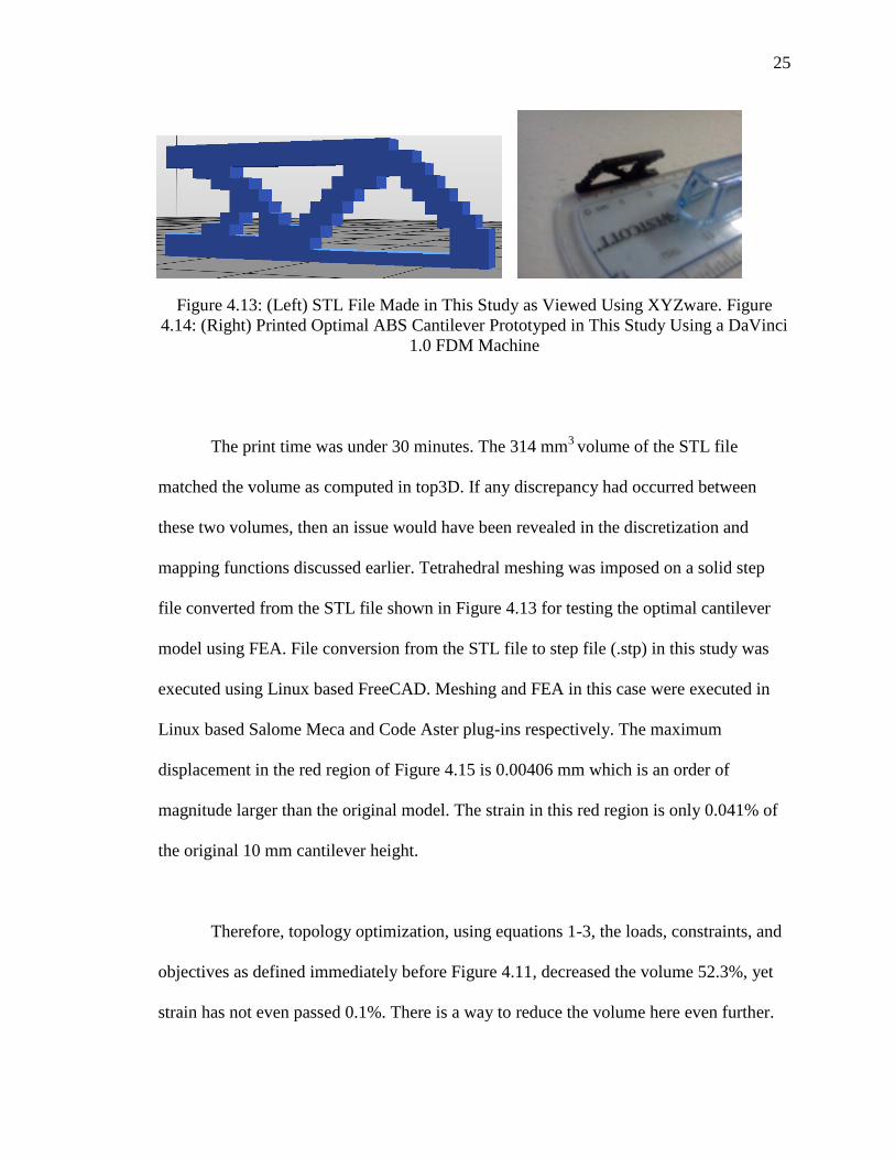
Figure 4.13: (Left) STL File Made in This Study as Viewed Using XYZware. Figure
4.14: (Right) Printed Optimal ABS Cantilever Prototyped in This Study Using a DaVinci
1.0 FDM Machine
The print time was under 30 minutes. The 314 mm3
volume of the STL file
matched the volume as computed in top3D. If any discrepancy had occurred between
these two volumes, then an issue would have been revealed in the discretization and
mapping functions discussed earlier. Tetrahedral meshing was imposed on a solid step
file converted from the STL file shown in Figure 4.13 for testing the optimal cantilever
model using FEA. File conversion from the STL file to step file (.stp) in this study was
executed using Linux based FreeCAD. Meshing and FEA in this case were executed in
Linux based Salome Meca and Code Aster plug-ins respectively. The maximum
displacement in the red region of Figure 4.15 is 0.00406 mm which is an order of
magnitude larger than the original model. The strain in this red region is only 0.041% of
the original 10 mm cantilever height.
Therefore, topology optimization, using equations 1-3, the loads, constraints, and
objectives as defined immediately before Figure 4.11, decreased the volume 52.3%, yet
strain has not even passed 0.1%. There is a way to reduce the volume here even further.
26
Figure 4.15: FEA Made in This Study of the Optimal Cantilever Prototype Model Using
Linux Based Software Salome Meca and Code Aster
Recalling the topology optimization results in a 3D array of moduli for each
voxel, and the moduli belong to a continuous range [0, E0]. The only means of writing the
STL file in Figure 4.13 was setting a binary threshold, so the moduli under the threshold
were eliminated leaving only moduli above the threshold in the model. Increasing the
threshold value slightly should eliminate slightly more material and cause a slightly
further reduction in the prototype’s volume without increasing the strain much.
A 40 mm x 20 mm x 40 mm simply supported platform was loaded with a 100N point
force in the top dead center as shown in Figure 4.16. The volume constraint Vs for
equation 1 was set to 0.5 or 50% of the 40 mm x 20 mm x 40 mm original volume.
Therefore, the objective was to find at most a 16000 mm3 design which supported the
100N distributed load while simply supported. The coordinates of the loads and
constraints are shared in Appendix K. The FEA displacement plot of this system shows
displacement existing primarily near the loading point in the red region of Figure 4.17.
Most of the platform was left un-strained as shown in the blue region. The maximum
27
displacement in the red region was 0.00000399 m in the z-direction only, and no buckling
was observable.
Figure 4.16: (Left) The Force Diagram for the Platform. Figure 4.17: (Right) The FEA
Plot of This Platform System Made in This Study Using Linux Based ImpactFEA
Regulated SIMP based topology optimization of the platform subject to the load,
constraints, and the objective volume constraint as defined immediately before Figure
4.16 removed 25616 mm3 from the original 32000 mm
3 design. The resulting 6384 mm
3
STL file shown in Figure 4.18 was printed during this study using a DaVinci 1.0 printer
to make the prototype shown in Figure 4.19. The ruler shown in juxtaposition with the
prototype of the optimal cantilever proves the topology optimization did not adversely
alter the scale of the 40 mm length dimension. The width and height dimensions are
preserved after the optimization as well, so any assembly fit requirements for this part are
still preserved.
The print time during this study was under 60 minutes for printing the prototype
in Figure 4.19 from the STL file in Figure 4.18 using a DaVinci 1.0 FDM machine. The
-100N
28
6384 mm3
volume of the STL file matched the volume as computed in top3D, so again,
the discretization and mapping functions which were made in this study and discussed
earlier were accurate.
Figure 4.18: (Left) STL File Made in This Study as Viewed Using XYZware. Figure
4.19: (Right) Printed Optimal ABS Platform Prototyped in This Study Using a DaVinci
1.0 FDM Machine.
Tetrahedral meshing was imposed on a solid step file converted from the STL file
shown in Figure 4.18 for testing the optimal cantilever model using FEA. File conversion
from STL to stp in this study was executed using Linux based FreeCAD. Meshing and
FEA in this case were executed in Linux based Salome Meca and Code Aster plug-ins
respectively. The maximum displacement in the red region is 0.0341 mm which is an
order of magnitude larger than the original model. The strain in this red region, shown in
Figure 4.20, is only 0.171% of the original 20 mm platform height.
29
Figure 4.20: FEA of the Optimal Platform Prototype Model Using Linux Based Software
Salome Meca and Code Aster
Therefore, topology optimization, using equations 1-3, the loads, constraints, and
objective function volume constraint as defined immediately before Figure 4.16,
decreased the volume 80%, yet strain had not even passed 0.1%. An in depth study of the
strain behavior required physical compression testing of this optimal 40 mm x 20 mm x
40 mm platform. Five platforms were printed using a DaVinci 1.0 FDM printer. The
DaVinci 1.0 prints quasi-hollow models using a honey comb lattice. Lattice density can
be varied using the XYZware software of the DaVinci 1.0. Density can range from 30%
to 90%. The 90% density setting was used in fabricating the platforms tested in this
study.
Each platform was placed on a level plane and compressive forces were added
using free weights to a top surface placed over the platform. An example compression
test setup was photographed and shown in Figure 4.21. The photographed platform was
optimized for a 100 N load, and the compression test range was 0 N to 178 N.
30
Compression occurred on the vertical axis of the platform. The initial height was 20 mm,
and initial load was 0 N.
Figure 4.21: An Example of the Compression Test Setup Employed in This Study.
The 40 mm x 20 mm x 40 mm optimal platform sits on a level surface under 44,497 N of
compressive weight.
A General UltraTech digital caliper with a resolution of 0.01 mm was used for
measuring the height of each platform three times for each compressive load. One inside
jaw was placed against the top level and the other inside jaw was rested against the
Caliper
measures the
difference
between the
upper and lower
levels.
Upper
Level
Lower
Level
Prototype
31
bottom level. The resulting measurement equals the height of the prototype under
compression. The average of three such height measurements for each prototype per
compressive load is shown in Table 4.3 and all the individual measurements are shared in
Appendix J.
Table 4.3: Compression Test Results
Compressive Force (N)
Average Height of
Prototype 1 after
compression
Average Height of
Prototype 2 after
compression
Average Height of
Prototype 3 after
compression
Average Height of
Prototype 4 after
compression
Average Height of
Prototype 5 after
compression
0 20.577 20.000 20.013 20.000 19.997
44.5 20.557 19.987 20.007 19.997 19.987
66.75 20.550 19.983 20.003 19.990 19.977
89 20.543 19.973 20.000 19.983 19.973
111.25 20.537 19.970 19.990 19.980 19.963
133.49 20.523 19.960 19.983 19.970 19.963
177.99 20.513 19.953 19.973 19.967 19.953
The results of compression testing in Table 4.3 are discussed in terms of stress-
strain behavior in Section 5.6.
The results of 40 mm x 20 mm x 40 mm optimization were scaled using a scale
factor of 5 to assess practicality of fabricating larger optimal objects. Scaling 5 times in
each direction made the 20 mm x 10 mm x 20 mm original design volume into a 200 mm
x 100 mm x 200 mm envelope. Meshing this new volume meant increasing the number of
32
voxels 125 times, yet the computational time required for optimization on this scale
would require 34 hours extrapolating from the results of Table 2. Scaling directly the
results of optimizing these small volumes required the development of scaletop3D
which scales the voxel moduli n x n x n array and returns a scaled sn/h x sn/h x sn/h array
where s is the scaling factor scale and h is the mesh discretization factor h_partition.
The scale is user defined in the function call for scaletop3D:
optmodel = scaletop3D(optmodel,scale, h_partition)
where the argument weight represents the modulus of each voxel element in the design
volume and the argument scale is a 1x3 vector representing the user’s desired 3D scale
factor for each direction. If the user enters a scale factor less than unity for any direction,
then scaletop3D does not work. The scale factor is used in this study for the purpose of
magnification only, so the expected value of each scale factor is greater than or equal to
unity. MATLAB does not directly provide a means for scaling 3D arrays like weight, so
the scaletop3d function replaces each voxel with its own s/h x s/h x s/h array named
del_V.
del_V = zeros(scale/h_partition(1),scale/h_partition(2),scale/h_partition(3));
for z=1:size(weight, 3)
for y=1:size(weight, 2)
for x = 1:size(weight, 1)
for z_scale = 1:scale/h_partition(3)
for y_scale = 1:scale/h_partition(2)
for x_scale = 1:scale/h_partition(1)
del_V(x_scale, y_scale, z_scale) =weight(x,y,z);
end
end
end
scaled_weight_arr{x,y,z}=del_V;
end
end
end
33
Every element of del_V equals the modulus of the previously single element from
the weight array. The single element has thus been successfully scaled. Each del_V array
is then stored in a structure, and then a new del_V array is made for the next voxel
element in weight. The resulting structure must be concatenated along all three
dimensions, so the result is transformation of the original 3D array into a structure and
finally into a scaled 3D array. Appendix C contains the full code required in this
transformation.
The number of elements in the scaled array is inversely proportional to the
discretization factor h_partition and directly proportional to the scaling factor scale.
The 704000 mm3 optimized platform occupies only 17.6% of the overall design
envelope’s volume as shown in Figure 4.22.
Figure 4.22: A 3D Scaled STL Made in This Study of the Optimal Platform Prototype
34
Finally, the capability of optstl to read in and optimize a pre-existing STL file
was tested. Figure 4.23 shows an example of a model FDM tool:
Figure 4.23: Example FDM Tool
An stl file was made after rendering a model of the tool shown in Figure 4.23. The
stl file image is shown in Figure 4.24. The length and width of the tool were modified to
4 inches by 6 inches, so the tool would fit inside the FDM platform of the DaVinci 1.0
printer used in this study.
Figure 4.24: STL File of the FDM Tool as Viewed in XYZware
35
The stl file shown in Figure 4.24 was loaded into the optimization engine using a
modified version of the publicly available VOXELISE MATLAB function. The modified
version of this function made as a result of this study is VOXELISE_FLEX:
function [gridOUTPUT,varargout] = VOXELISE_FLEX(gridX,gridY,gridZ,
discretization, filename)
where gridX, gridY, and gridZ are the overall x, y, and z dimensions of the model
rounded up to the nearest millimeter, filename is the file path of the STL model, and
discretization is the number of voxel lengths per millimeter. A discretization
factor of 1 would produce a mesh of 1 voxel per mm3. Voxelising the stl shown in Figure
4.24 using a discretization factor of 1 yielded 875000 voxels. The stl file was then scaled
down by a factor of 10 on each side, so the discretization factor could be increased and
computation time decreased. Figure 4.25 shows an image of the voxelised model before
optimization.
Figure 4.25: Voxelised FDM Tool as Viewed in the MATLAB Figure Window
36
A 100N point force and simply supported constraints were placed on the model as
shown in Figure 4.26, and the volume constraint, Vs, for the objective function in
equation 1 was set 0.5 meaning 50% of 30 mm x 48 mm x 15 mm envelope of the design.
The locations of the loads and constraints are shared in Appendix K :
Figure 4.26: FDM Tool Load and Constraint Diagram
Figure 4.13 and 4.18 show the optimized model to have significantly different
surface topology from the original model of each. Surfaces are often key components in a
products function, so preserving the surface of the top and sides of the tool was studied.
A boundaryelements function was written to find all the voxels on the top and sides of
a model:
function boundaryelements = findboundary(gridOUTPUT, nelx, nely, nelz)
where gridOUTPUT, nelx, nely, and nelz are the original voxelised model, the
number of elements in the x direction, the number of elements in the y direction ,and the
number of elements in the z direction. Three Booleans are used to determine whether a
-100N
37
voxel is on the boundary of the model. First, the voxels at the bounds of the design
volume can be found using this Boolean:
(gridOUTPUT(i,j,k)==1)&& ((i~=length(nelx) || (i==length(nelx) &&
((j==1) || (j==length(nely)) || (k==1) || (k==length(nelz))))))
Voxels not at the boundary of the design volume yet at the boundary of the model can be
found using these two Booleans in order:
gridOUTPUT(i,j,k)==1) && (i~=1) && (i~=length(nelx)) && (j~=1) &&
(j~=length(nely)) && (k~=1) && (k~=length(nelz))
gridOUTPUT(i+1,j,k)==0 || gridOUTPUT(i-1,j,k)==0 ||
gridOUTPUT(i,j+1,k)==0 || gridOUTPUT(i,j,k+1)==0 ||gridOUTPUT(i,j,k-
1)==0
Figure 4.27 shows the resulting optimized model which from the top and sides is
identical to topology of the original voxelised model in Figure 4.26. The resulting STL
file was scaled up by a factor of 10 in each direction to produce the topologically
optimized STL of the original STL shown in Figure 4.26. Figure 4.28 reveals the optimal
interior of the model.
Figure 4.27: (Left) Optimized FDM Tool as Viewed in a MATLAB Figure Window.
Figure 4.28: (right) Optimized FDM Tool as Viewed at an Angle in XYZware.
38
5. DISCUSSION
5.1 CAPABILITY OF A SINGLE INTERFACE
The optstl interface provides a vast array of STL modification functions:
meshing via VOXELISE_FLEX, mapping via generate_cube_m, topology optimization via
top3dFlex, scaling transformation via scaletop3D, binary homogenization via
optcoordinates, user input/output, point cloud generation, and stl writing. The
VOXELISE_Flex function was adapted and modified from the publicly available
VOXELISE Matlab function. Modifications to this function include the ability for the user
to change the discretization factor and mesh density in the x, y, and z direction
individually. The generate_cube_m was made originally in this study for trilinear
discretization of the design volume for mapping into the optimization engine. The
top3dFlex function was modified from the top3d function, so user no longer needs to
know parametric functions to describe the surface of the input design volume. The
original top3d function required explicit parameterized representation of the design
volume’s surface to map loads and constraints. Explicit parameterization of more
complex design volume may not be feasible, so the modified top3dFlex function was
developed in this study to allow a user to input just the Cartesian coordinates of the loads
and constraints. Optimization increased the point cloud computation time by a minimum
factor of 170 times, so a scaletop3D function was developed in this study to allows a
user to optimize a small scale system and the scale up the results. Getting the results of
the topology optimization required homogenization from the continuous distribution of
moduli to a binary distribution, so the optcoordinates function was made originally in
39
this study to find all the vertices of voxels which met and did not meet a threshold value.
Voxels which met the threshold value were assigned a 1, and voxels which did not meet
the threshold value were assigned a 0. The optstl script passes this binary homogenized
data into a copy of the publicly available dxfpoint function for generation of a point. A
copy of the publicly available CONVERT_voxels_to_stl MATLAB function similarly
interprets the binary distribution of voxels as those voxels with a 0 value were outside the
stl while voxels with a 1 value were inside the stl.
5.2 TOP3DFLEX
Two of the three examples accompanying the top3D software were tested
and worked successfully for this study. One example was the cantilever beam and the
second was a platform [18]. The loads were changed in this study for testing the
practicality of the software in fabricating ABS prototypes. The cantilever load in this
study was a -100 N/mm distributed load putting the tip in shear, and the platform load in
this study with a -100 N point force in the center of the platform. The Young’s modulus
used for ABS was 2150 MPa, and a table of the material properties appears in Appendix
I. Liu and Tovar used a Young’s modulus of 1 MPa and load magnitudes of -1N/mm and
-1N for the cantilever and platform respectively [18]. The topology optimization
produced a 58.3% reduction in cantilever’s volume and a 92% reduction in the platform’s
volume. Liu and Tovar’s software required the user to adjust values directly within the
script [19]. The top3dFlex script operates within the optstl main script, so the user is
allowed to input values for the Young’s modulus, loads, and constraints on a case by case
basis without risking corruption of the optimization engine. The loads and constraints of
40
Liu and Tovar’s script required surface parameterization [19]. The optstl main script
has user input/output which allows the user to input only the Cartesian coordinates of the
loads and constraints, and then optstl maps these coordinates to voxel vertices using the
trilinear discretization information of the generate_cube_m function. The optstl main
script then passes these arguments directly into the top3dFlex script. The potential for
the user to input large stl files for topology optimization meant a large number of voxel
elements could be involved in the computation. Liu and Tovar discussed a fast iterative
solver option for top3d [19], so top3dFlex included this iterative solver as a default
solver.
5.3 MESHING, DISCRETIZATION, AND MAPPING
A user can now directly input any design volume via stl such as FDM tool model
shown in Figure 4.23 to voxelized as shown in Figure 4.24 for input into the optimization
engine. The VOXELISE_Flex function reads and meshes the input stl file as a 3D array of
elements. The original VOXELISE function assigns 0’s to all voxels in the design volume
yet outside the stl and 1’s to all the voxels inside the stl. Each voxel from the VOXELISE
function represented 1 mm3 of the model. Modifying the 1mm
3 mesh density may be a
user priority especially when working with complex surface geometry, so the
VOXELISE_Flex function was developed in this study. Mesh density in the
VOXELISE_Flex function is determined using a user defined discretization factor where
the user is allowed to input the number of voxels required per millimeter.
41
The meshed design volume from the VOXELISE_Flex function is passed through
optstl for mapping the user defined loading and constraints. User defined Cartesian
coordinates of the loads and constraints are mapped to mesh indices using the
generate_cube_m function. The first voxel in the system is located in the top back left
and the last voxel is location in the bottom front left. Indexing first traverses top to
bottom, then left to right, and finally back to front. Trilinear discretization in the
generate_cube_m mapping algorithm was tested for two abilities. Simply mapping
indices of all the voxel vertices in the design volume and connecting the vertex indices in
order to create each associated voxel was one test. Figure 4.4 and Figure 4.5 proved the
generate_cube_m function with optcoordinates can correctly map the topology
optimization results from MATLAB figures to voxels for the stl files. The second feature
tested was the capacity for adjusting the mesh fineness. Figures 4.4 and 4.5 illustrated the
different discretization and mesh density possible through manipulation of the
h_partition argument in generate_cube_m. Varying the values of h_partition
indirectly varies the mesh density, so low values of h_partition create the most dense
voxel meshes.
5.4 SCALING
Figure 4.22 illustrated the ability of optstl to scale an optimized model.
Successfully overcoming the problem of scale here required the implementation of a
scaling algorithm. MATLAB only has a scaling algorithm for 2D arrays, yet users can
require scaling length, width, and height dimensions simultaneously. The scaling of each
dimension was accomplished using scaletop3D. Any 3D array can be scaled using this
42
function, and the output mesh density can be adjusted using the user defined
h_partition. Adjusting the value of h_partition indirectly changes the mesh density just
the like in the case of generate_cube_m.
5.5 STL WRITING
Figures 4.13, 4.18, and 4.28 illustrated optstl’s ability to write stl files. A 3D
array of 1’s and 0’s is passed via optstl to the publicly available
CONVERT_voxels_to_stl function. The 1’s indicate a voxel element is located within the
model while the 0’s indicate the voxel element is outside the model. All of the voxel
elements are processed through a set of binary homogenization instructions from the
optimization engine. Binary homogenization is the process of preparing the data for the
stl writing function. Processing the data is a matter of having a set binary homogenization
threshold value as discussed in paragraphs preceding Figure 4.7-4.10. Images for Figures
4.13, Figure 4.18, and Figure 4.28 use a binary homogenization threshold of 0.5.
Topology optimization produced a 3D array with a continuous distribution of moduli
from [0, E0] where E0 is the Young’s modulus of the material used in fabrication. Finding
all of the resulting values above the threshold and setting these values equal to 1
determined the interior of the stl models. Values below the threshold were set to 0
determining the outside of the stl models. Completing the binary homogenization was the
last step required before writing the stl files.
5.6 TOPOLOGICALLY OPTIMIZED SOLID FREEFORM FABRICATION
The STL for each optimal model example was printed successfully during this
study as illustrated in Figure 4.14 and Figure 4.19. A DaVinci 1.0 printer extruding ABS
43
filament was used in fused deposition modeling of each print in this study. None of these
prototypes required over 1 hour to print. Volumes for each printed model matched the
volumes of the computed models revealing no error in the discretization, meshing, and
mapping functions discussed earlier. Testing the integrity of the printed STL was
paramount after analyzing the FEA plots of the optimized models. Each model showed
less than 0.1% strain after optimization as illustrated in Figure 4.15 and Figure 4.20.
Only physical testing could validate the true mechanical compliance evident in these
results, so the printed optimal ABS platform was subjected to compression testing. Data
from this compression test was shared in Table 4.3, and the raw data is shared in
Appendix J. Table 5.1 and Figure 5.1 display the prototype’s behavior under
compression, the theoretical behavior based on the Young’s modulus of ABS, and a light
blue line indicates the design load of 100 N.
Strains were calculated for each data point from Table 4.3 was calculated using
Eq 10:
(Eq 10)
where the ith strain value is the difference between the prototype’s initial height h0 and
the height after the ith load divided by the prototype’s initial height h0. Forces from Table
5.1 are the numerator for the stress calculated in Pascals for Figure 5.1 using Eq 11:
(Eq 11)
where the ith stress value is the ratio of the ith compressive force to the prototype’s
constant load bearing surface area, A = 4.75 x 10⁻⁴
m3. Substituting values for each load
44
into Eq 5 produces the control strain distribution shown in the second column of Table
5.1:
(Eq 12)
where the ith control strain is the ratio of the ith strain to the constant Young’s
modulus of ABS, E = 2150 MPa. The results were tabulated in Table 5.1.
Table 5.1 Prototype Compression Test Stress and Strain Results
Compressive force (N)
Control Strain
Strain 1 Strain 2 Strain 3 Strain 4 Strain 5
0 0 0 0 0 0 0
4.450E+01 2.069E-08
0.001 6.667E-
04 3.331E-04 1.667E-04
5.001E-04
6.675E+01 3.104E-08
1.296E-03
8.333E-04
4.997E-04 5.000E-04 1.000E-
03
8.900E+01 4.139E-08
0.002 1.333E-
03 6.662E-04 8.333E-04
1.167E-03
1.112E+02 5.174E-08
1.944E-03
1.500E-03
1.166E-03 1.000E-03 1.667E-
03
1.335E+02 6.209E-08
2.592E-03
2.000E-03
1.499E-03 1.500E-03 1.667E-
03
1.780E+02 8.278E-08
3.078E-03
2.333E-03
1.999E-03 1.667E-03 2.167E-
03
The calculated values from Table 5.1 are plotted in Figure 5.1, so the typical
compression behavior can be observed. Compression testing occurred in the elastic
region of ABS, so the Young’s modulus could be chosen a control. The plot in Figure 5.1
shows the compression testing stress strain behavior of the five prototypes. One line in
Figure 5.1 shows the theoritical stress-strain behavior as modelled using Young’s
modulus, and another line shows the stress-strain behavior as predicted using the FEA in
45
Figure 4.20. No fractures were observed after the final load step. Wave like behavior in
Figure 5.1 is attributed to the experiment setup and instrument resolution in Figure 4.21.
Figure 5.1: The ABS Prototype’s Performance vs the Young’s Modulus of ABS and the
Computed FEA Result
The FEA shown in Figure 4.20 computed that the maximum strain should be
0.171%. A one sample t-test of the compression test data near the design load at
234,082.6 Pa yielded a t value of -2.615. If t < tcritical,α for the one-sided one sample t-test,
then there is a statistical directional difference from the expected mean value. A one-
tailed 95% confidence tcritical,α one tailed value computed in MS Excel was -2.132, so the
compression testing results were significantly less than the FEA’s result with 95%
confidence. However, the one tailed 99% confidence tciritical,α value computed in MS
0
50000
100000
150000
200000
250000
300000
350000
400000
0 0.0005 0.001 0.0015 0.002
Stre
ss (
Pa)
Strain
Compression Test for ABS Prototypes
E = 2.15 GPa
Prototype 1
Design Load
Prototype 2
Prototype 3
Prototype 4
Prototype 5
FEA
46
Excel was -3.747, so the differences between the prototypes and FEA are not signficantly
different at the 99% confindence level.
The test was selected for testing the difference between the observed
prototypes’ behavior under compression and the Young’s modulus as shown in Table 5.2.
If the p-value is less than 0.01, then the two behaviors are different with 99.99%
confidence.
Table 5.2: p-values for χ^2 Test Comparison of Each Prototype Sample Against
the Expected Behavior from Young’s Modulus
Prototype #
p-Value of χ^2 Comparison
Prototype and Control
1 6.24947E-97
2 3.15124E-54
3 2.24923E-27
4 3.13694E-23
5 3.33495E-48
All of the p-values are less than 0.01, so the prototypes’stress-strain behavior
under compression was signfiantly different from the Young’s modulus. The reason for
this difference is the change in cross sectional area. Cross sections of the control
modelled using Young’s modulus were uniform while the cross sections of the prototype
shown in Figure 4.18 are non-uniform. The second area moment of inertia is directly
proportional to cross sectional area and measures the amount of resistance an object may
have to a given static load. Therefore, decreasing cross sectional areas from the model in
47
the prototype reduced the second area moment of inertia in the prototype and caused the
decrease in the stress-strain relationship from the Young’s modulus behavior.
5.7 ADAPTIVE PLACEMENT OF USER DEFINED LOAD(S) AND
CONSTRAINT(S) ON USER DEFINED VOLUMES
Images shown in Figures 4.2-4.5, 4.7-4.10, 4.13-4.14, 4.18-4.19, 4.22 and 4.27-
4.28 were all made in this study using optstl. The optstl loading and constraint
instructions allow the user to input Cartesian coordinates of loads and constraints.
Loading this information using coordinates is not permitted in the original top3d. Load
and constraint information in top3d required explicit surface parameterization meaning
the user had to know how to calculate the index of a voxel at an (x,y,z) coordinate. Using
optstl the user can input just (x,y,z) coordinate of a point load or constraint, and the
optstl alogorithm uses the generate_cube_m function made in this study. Use of the
generate_cube_m function generates both a list of all the (x,y,z) voxel vertice
coordinates in the design volume and a list of the order in which to connect these
vertices. Trilinear discretization dictates the programmed order in which these vertices
are connected to produce the voxelized space. Surface constraints and uniformly
distributed loads can be applied as well. If the user wishes, then optstl holds a user
defined dimension constant in order to load or constrain an entire 2D plane of active
voxels. Active voxels were stored in the memory as voxel elements with a value of
1using the binary homogenization instructions of optcoordinates discussed earlier.
Passive voxels would have a value of 0. Setting loads and constraints based on Cartesian
coordinates simplifies the surface parameterization step. A resulting list of loaded and
constrained vertices are passed to top3dFlex along with the Young’s modulus and an
48
array of passive elements. Passing the passive elements into the topology optimization
engine forces the computation to retain any features such as holes [19]. Large quantities
of passive or active elements could cause long computation times [19], so the top3dFlex
algorithm was adapted to implement the MATLAB pcg solver. Liu and Tovar
recommended the pcg solver for the fastest computation speed [19]. Implementing the
pcg solver allows MATLAB to determine the best solution for system of linear equations
at hand. Adapting top3d into top3dFlex and supplementing this function using the
optstl main script decreases the amount of hard coding the user must do in order to
modify the program to differenct design requirements. Supplementing the script further
with an STL reading function allows the user to load and constrain any design volume.
Figure 4.17 demonstrates the ability of any STL to be voxelized for input into the
optimization engine. If the model’s function requires that certain voxels be preserved
such as the outermost layer of voxels, then the boundaryelements function can be used
as demonstrated in Figure 4.28.
49
6. CONCLUSION
The fabrication of topologically optimized parts is realizable using optstl .
Topology optimization was shown in this study to produce parts of significantly less
elastic modulus than unoptimized parts of the same load and constraint parameters. ABS
parts were fabricated in this study using optstl and a DaVinci 1.0 FDM machine.
Fabrication required the adaption of Liu and Tovar’s top3d algorithm and several
supplemental functions. Adapting the top3d algorithm resulted in a user input/output
interface for optimizing any stl input subject to user defined load and constraint
coordinates. Output from this adapted program named optstl can be a scaled model,
point cloud, and/or an stl file. Each optimized prototype was analyzed using FEA, and
one optimized prototype was subjected to compression testing. Supplemental FEA’s of
the original models are shared in Appendix H. An order of magnitude increase in the
strain was observed in the optimized prototypes when compared with the original models.
Statistical testing of the compression test results did reveal a significant statistical
difference between a theoretical solid ABS volume’s behavior and the optimized
prototype’s behavior. The actual stress-strain behavior resembles that as predicted in the
FEA result in Figure 4.20.
Solid freeform fabrication users now have a MATLAB preprocessor for loading,
optimizing, and writing the STL’s of design volumes. Unification of these engineering
design processes is provided in optstl. The publicly available top3D, VOXELISE, and
CONVERT_voxels_to_stl algorithms were found, modified, and coalesced
50
algorithmically in optstl. Added functionality such as scaling, discretization, binary
homogenization, and user defined volumes required supplemental functions and
modifications of the pre-existing function arguments. Adjusting a 3D array’s scale was a
matter of applying fundamentals from the 1D and 2D mathematical transformations for
the scaletop3D function. All of the results produced in this study can be scaled using a
scaling algorithm for 3D MATLAB arrays developed successfully during this study.
Optimizing the smaller design envelope and then scaling the result can save computation
time of a large volume. MATLAB did not previously have a 3D scaling function in the
MATLAB library or on the internet. Using MATLAB structures, arrays, and
concatenation in a combination of nested for loops yielded the sufficient scaling
transformation for this study. Mapping required knowledge of FEA techniques for
solving partial differential equations in a trilinear discretized system for the
generate_cube_M function. Trilinear discretization produces finite element mesh
comprised of cubes which can map 1 to 1 with voxels. Indexing the trilinear discretized
mesh for this study was already discussed in Liu and Tovar’s paper, so the indexing
process was simply automated for user’s of optstl. Automating and storing the index
data mapping of the voxelized system enables the user to input an (x,y,z) coordinate and
return an array element index for the optimization functions. Allowing the user to
communicate using the Cartesian coordinate system simplifies the process of translating
the real data into the computer, for example a user could use CMM or point cloud data.
All of optstl is written in MATLAB. Core components of optstl are shared in
Appendix A- Appendix D, and converting these scripts to a C based programming
language or parallel computing algorithms can increase computation speed.
51
The optstl package coalesced the functions of model loading, constraining,
topology optimization, scaling, mapping, and stl writing. Using optstl for solving
equations 1-3 for design volumes did reduce the amount of raw material required for the
fabrication of load bearing structures. Material costs and fabrication times were in turn
reduced because of the decrease in the volume and amount of material required.
Compression testing showed that the optimized parts deformed significantly more than
unoptimized parts, yet each prototype in this study did support its design load. Any user
defined stl could be optimized using equations 1-3, loads, and simply supported
constraints in optstl, and the function of the model could be preserved using the
boundaryelements function of optstl.
53
%%%%%%%%%%%%%%%%%%%%%%%%%%%%%%%%%%%%%%%%%%%%%%%%%%%%%%%%%%%%%%%%%%%%%%%
%%% %%Purnajyoti Bhaumik wrote this for topology optimization of any 3D
model
function optstl
prompt = 'Would you like to input an STL file or optimize a rectangular
prism? Enter Y or N. '; source_type = input(prompt,'s'); if isempty(source_type) return end if source_type == 'Y' prompt = 'What is the source STL filename (include file path and
extension ex: C:\test.stl)? '; STLin = input(prompt,'s'); if isempty(STLin) return end gridX = input('What is the overall height (in mm)?'); if isempty(gridX) return end
gridY = input('What is the overall width (in mm)?'); if isempty(gridY) return end
gridZ = input('What is the overall depth (in mm)?'); if isempty(gridZ) return end end
if source_type == 'N' gridX = input('What is the overall width (in mm)?'); if isempty(gridX) return end
gridY = input('What is the overall height (in mm)?'); if isempty(gridY) return end
gridZ = input('What is the overall depth (in mm)?'); if isempty(gridZ) return end
54
nelx = 1:1:gridX; nely = 1:1:gridY; nelz = 1:1:gridZ;
for k = 1:gridZ for i = 1:gridX for j = 1:gridY gridOUTPUT(i,j,k) = 1; end end end %gridOUTPUT(:,:,:)=1; gridOUTPUT= permute(gridOUTPUT, [2,1,3]); display_3D(gridOUTPUT) end
if source_type == 'Y' prompt = 'How many voxels per millimeter? '; discretization = input(prompt); if isempty(discretization) returns end [gridOUTPUT,nely,nelx,nelz] = VOXELISE_FLEX(gridX, gridY, gridZ,
discretization,STLin); gridX = length(nelx); gridY = length(nely); gridZ = length(nelz); display_3D(gridOUTPUT) end
passive = find(~gridOUTPUT); active = find(gridOUTPUT);
[M, T] = generate_cube_M(0, length(nelx), 0, length(nely), 0,
length(nelz), [1,1,1],1);
load_answer = 'Y'; i=0; while load_answer == 'Y' prompt = 'Would you like a distributed load or a point force? Enter D
or P: '; load_type = input(prompt, 's'); if isempty(load_type) return end i = i+1; if load_type == 'D' prompt = 'Would you like this load distributed in a perpindicular
to the width, depth, or height of the model? Enter w, d, or h: '; load_plane = input(prompt, 's'); if load_plane == 'h' prompt = ('At what distance from the bottom would you like
this distributed load? Enter this distance in whole millimeters.'); load_plane_width = input(prompt);
55
if isempty(load_plane_width) return end for z = 1:gridZ for x = 1:gridX for m = 1:length(active) if active(m)== load_plane_width+(x-
1)*(gridY)+(z-1)*(gridY*gridX) loadnid{i} =
unique(T([5,6,7,8],active(m))); i = i+1; end end end end i = i-1; elseif load_plane == 'd' prompt = ('At what distance from the back would you like
this surface constraint? Enter this distance in whole millimeters.'); load_plane_width = input(prompt); if isempty(load_plane_width) return end for x = 1:gridX for y = 1:gridY for m = 1:length(active) if active(m)==(x-
1)*gridY+y+load_plane_width*(gridY*gridZ) loadnid{i} =
unique(T([1,2,7,8],active(m))); i = i+1; end end end end i = i-1; elseif load_plane == 'w' prompt = ('At what distance from the left would you like
this surface constraint? Enter this distance in whole millimeters.'); load_plane_width = input(prompt); if isempty(load_plane_width) return end for z = 1:gridZ for y = 1:gridY for m = 1:length(active) if active(m)==(z-
1)*(gridX*gridY)+y+load_plane_width*gridY loadnid{i} =
unique(T([1,4,5,8],active(m))); i = i+1; end end end end i = i-1;
56
end elseif load_type == 'P' prompt = ('You will be asked for the 3D coordinates of this point
force. What is the x-coordinate in millimeters?'); pforcex = input(prompt); prompt = ('What is the y-coordinate in millimeters?'); pforcey = input(prompt); prompt = ('What is the z-coordinate in millimeters?'); pforcez = input(prompt); for k = 1:size(M,2) if M(1,k)==pforcex && M(2,k)==pforcey && M(3,k)==pforcez loadnid{i} = k; end end end prompt = ('Would you like to enter another load? Enter Y or N'); load_answer = input(prompt, 's'); if isempty(load_answer) return end end
final_load = loadnid{1}; for j = 2:i final_load = cat(1, final_load, loadnid{j}); end
prompt = 'What is the magnitude of the load?'; load_mag = input(prompt); if isempty(load_mag) return end
constraint_answer = 'Y'; i=0; while constraint_answer == 'Y' prompt = 'Would you like a surface or a point constraint? Enter S or P:
'; constraint_type = input(prompt, 's'); if isempty(constraint_type) return end i = i+1; if constraint_type == 'S' prompt = 'Would you like this load distributed perpindicular the
width, depth, or height of the model? Enter w, d, or h: '; constraint_plane = input(prompt, 's'); if constraint_plane == 'h' prompt = ('At what distance from the bottom would you like
this surface constraint? Enter this distance in whole millimeters.'); constraint_plane_width = input(prompt); if isempty(constraint_plane_width) return end for z = 1:gridZ for x = 1:gridX
57
for m = 1:length(active) if active(m)== constraint_plane_width+(x-
1)*(gridY)+(z-1)*(gridY*gridX) constraintnid{i} =
unique(T([5,6,7,8],active(m))); i = i+1; end end end end i = i-1; elseif constraint_plane == 'd' prompt = ('At what distance from the back would you like
this surface constraint? Enter this distance in whole millimeters.'); constraint_plane_width = input(prompt); if isempty(constraint_plane_width) return end for x = 1:gridX for y = 1:gridY for m = 1:length(active) if active(m)==(x-
1)*gridY+y+constraint_plane_width*(gridY*gridZ) constraintnid{i} =
unique(T([1,2,7,8],active(m))); i = i+1; end end end end i = i-1; elseif constraint_plane == 'w' prompt = ('At what distance from the left would you like
this surface constraint? Enter this distance in whole millimeters.'); constraint_plane_width = input(prompt); if isempty(constraint_plane_width) return end for z = 1:gridZ for y = 1:gridY for m = 1:length(active) if active(m)==(z-
1)*(gridX*gridY)+y+constraint_plane_width*gridY constraintnid{i} =
unique(T([1,4,5,8],active(m))); i = i+1; end end end end i = i-1; end elseif constraint_type == 'P' prompt = ('You will be asked for the 3D coordinates of this point
force. What is the x-coordinate in millimeters?'); pconstraintx = input(prompt);
58
prompt = ('What is the y-coordinate in millimeters?'); pconstrainty = input(prompt); prompt = ('What is the z-coordinate in millimeters?'); pconstraintz = input(prompt); for k = 1:size(M,2) if M(1,k)==pconstraintx && M(2,k)==pconstrainty &&
M(3,k)==pconstraintz constraintnid{i} = k; end end; end prompt = ('Would you like to enter another constraint? Enter Y or N'); constraint_answer = input(prompt, 's'); if isempty(constraint_answer) return end end
final_constraint = constraintnid{1}; for j = 2:i final_constraint = cat(1, final_constraint, constraintnid{j}); end final_constraint = unique(final_constraint);
t = cputime
prompt = ('What is the modulus of elasticity in MPa?'); Young_answer = input(prompt); if isempty(Young_answer) return end
active = findboundary(gridOUTPUT, nely, nelx, nelz); test = gridOUTPUT; test(~active) = 0; test(active) = 1; clf; display_3D(test) optmodel = top3dFlex(length(nelx),length(nely),length(nelz), 0.3, 3,
1.5, final_load, final_constraint, passive, Young_answer,
load_mag,active);
prompt = ('Would you like to scale this model? Please enter Y or N'); scale_answer = input(prompt, 's'); if isempty(scale_answer) return end
if scale_answer == 'Y'
59
prompt = 'How many voxels per millimeter? (recommended at least 1
voxel per millimeter) '; discretization = input(prompt); if isempty(discretization) return end
prompt = ('Please enter a scale factor for the x-axis: Only whole
numbers greater than or equal to 1'); x_scale = input(prompt); if isempty(x_scale) return end for i = 1:x_scale*length(nelx)/discretization nelx(i) = min(nelx)+(i-1)*(discretization); end prompt = ('Please enter a scale factor for the y-axis: Only whole
numbers greater than or equal to 1'); y_scale = input(prompt); if isempty(y_scale) return end for i = 1:y_scale*length(nely)/discretization nely(i) = min(nely)+(i-1)*(discretization); end prompt = ('Please enter a scale factor for the z-axis: Only whole
numbers greater than or equal to 1'); z_scale = input(prompt); if isempty(z_scale) return end for i = 1:z_scale*length(nelz)/discretization nelz(i) = min(nelz)+(i-1)*(discretization); end scale = [x_scale, y_scale, z_scale]; h_partition = [discretization, discretization, discretization]; optmodel = scaletop3D(optmodel,scale, h_partition) end
opt_passive = find(optmodel<=0.5); opt_active = find(optmodel>0.5); optmodel(opt_passive) = 0; optmodel(opt_active) = 1; optmodel(active) = 1; clf; display_3D(optmodel)
prompt = ('Would you like to make a point cloud? Please enter Y or N'); cloud_answer = input(prompt, 's'); if isempty(cloud_answer) return elseif cloud_answer == 'Y' point_cloud = optcoordinates(M,T, optmodel) prompt = ('What is the destination dxf filename (include file path
and extension ex: C:\test.dxf)? '); cloud_answer = input(prompt, 's');
60
if isempty(cloud_answer) return end FID = dxf_open(cloud_name); dxf_point(FID,point_cloud(3,:), point_cloud(1,:),
point_cloud(2,:)); dxf_close(FID); end
prompt = ('Would you like to make an STL file? Please enter Y or N'); stl_answer = input(prompt, 's'); if isempty(stl_answer) return elseif stl_answer == 'Y' prompt = ('What is the destination STL filename (include file path and
extension ex: C:\test.stl)? '); STLout = input(prompt,'s'); CONVERT_voxels_to_stl(STLout, optmodel, nely, nelx, nelz,'ascii'); end cputime - t end % DISPLAY 3D TOPOLOGY (ISO-VIEW)is copied from Liu and Tovar's top3d function display_3D(rho) [nely,nelx,nelz] = size(rho); hx = 1; hy = 1; hz = 1; % User-defined unit element size face = [1 2 3 4; 2 6 7 3; 4 3 7 8; 1 5 8 4; 1 2 6 5; 5 6 7 8]; set(gcf,'Name','ISO display','NumberTitle','off'); for k = 1:nelz z = (k-1)*hz; for i = 1:nelx x = (i-1)*hx; for j = 1:nely y = nely*hy - (j-1)*hy; if (rho(j,i,k) > 0.5) % User-defined display density
threshold vert = [x y z; x y-hx z; x+hx y-hx z; x+hx y z; x y
z+hx;x y-hx z+hx; x+hx y-hx z+hx;x+hx y z+hx]; vert(:,[2 3]) = vert(:,[3 2]); vert(:,2,:) = -
vert(:,2,:);
patch('Faces',face,'Vertices',vert,'FaceColor',[0.2+0.8*(1-
rho(j,i,k)),0.2+0.8*(1-rho(j,i,k)),0.2+0.8*(1-rho(j,i,k))]); hold on; end end end end axis equal; axis tight; axis off; box on; view([30,30]); pause(1e-6); end
62
%P. Bhaumik's Oct 2014 optimization code based on code by LIU AND TOVAR
(JUL 2013) function xPhys = top3dFlex(nelx,nely,nelz,volfrac,penal,rmin, loadnid,
fixednid,passive, Young, load_mag,active) % USER-DEFINED LOOP PARAMETERS maxloop = 200; % Maximum number of iterations tolx = 0.01; % Termination criterion displayflag = 1; % Display structure flag % USER-DEFINED MATERIAL PROPERTIES E0 = Young; % Young's modulus of solid material titanium
alloy Emin = 1e-9; % Young's modulus of void-like material nu = 0.3; % Poisson's ratio % USER-DEFINED LOAD DOFs loaddof = [3*loadnid(:) - 1]; % DOFs % USER-DEFINED SUPPORT FIXED DOFs fixeddof = [3*fixednid(:); 3*fixednid(:)-1; 3*fixednid(:)-2]; % DOFs % PREPARE FINITE ELEMENT ANALYSIS nele = nelx*nely*nelz; ndof = 3*(nelx+1)*(nely+1)*(nelz+1); F = sparse(loaddof,1,load_mag/size(loadnid,1),ndof,1); U = zeros(ndof,1); freedofs = setdiff(1:ndof,fixeddof); KE = lk_H8(nu); nodegrd = reshape(1:(nely+1)*(nelx+1),nely+1,nelx+1); nodeids = reshape(nodegrd(1:end-1,1:end-1),nely*nelx,1); nodeidz = 0:(nely+1)*(nelx+1):(nelz-1)*(nely+1)*(nelx+1); nodeids = repmat(nodeids,size(nodeidz))+repmat(nodeidz,size(nodeids)); edofVec = 3*nodeids(:)+1; edofMat = repmat(edofVec,1,24)+ ... repmat([0 1 2 3*nely + [3 4 5 0 1 2] -3 -2 -1 ... 3*(nely+1)*(nelx+1)+[0 1 2 3*nely + [3 4 5 0 1 2] -3 -2 -
1]],nele,1); iK = kron(edofMat,ones(24,1))'; jK = kron(edofMat,ones(1,24))'; % PREPARE FILTER iH = ones(nele*(2*(ceil(rmin)-1)+1)^2,1); jH = ones(size(iH)); sH = zeros(size(iH)); k = 0; for k1 = 1:nelz for i1 = 1:nelx for j1 = 1:nely e1 = (k1-1)*nelx*nely + (i1-1)*nely+j1; for k2 = max(k1-(ceil(rmin)-1),1):min(k1+(ceil(rmin)-
1),nelz) for i2 = max(i1-(ceil(rmin)-1),1):min(i1+(ceil(rmin)-
1),nelx) for j2 = max(j1-(ceil(rmin)-
1),1):min(j1+(ceil(rmin)-1),nely) e2 = (k2-1)*nelx*nely + (i2-1)*nely+j2; k = k+1; iH(k) = e1; jH(k) = e2;
63
sH(k) = max(0,rmin-sqrt((i1-i2)^2+(j1-
j2)^2+(k1-k2)^2)); end end end end end end H = sparse(iH,jH,sH); Hs = sum(H,2); % INITIALIZE ITERATION x = repmat(volfrac,[nely,nelx,nelz]); x(passive)=0; xPhys = x; loop = 0; change = 1; % START ITERATION while change > tolx && loop < maxloop loop = loop+1; % FE-ANALYSIS sK = KE(:)*(Emin+xPhys(:)'.^penal*(E0-Emin)); K = sparse(iK(:),jK(:),sK(:)); K = (K+K')/2; tolit = 1e-8; maxit = 8000; %M = diag(K); M = diag(diag(K(freedofs, freedofs))); U(freedofs,:)=pcg(K(freedofs, freedofs),F(freedofs,:), tolit, 1000,
M); %[num_nodes, num_loads] = size(U); % for i = 1:num_loads % U(freedofs,i)=pcg(K(freedofs, freedofs),F(freedofs,i), tolit,
1000, M); % end % OBJECTIVE FUNCTION AND SENSITIVITY ANALYSIS ce = reshape(sum((U(edofMat)*KE).*U(edofMat),2),[nely,nelx,nelz]); c = sum(sum(sum((Emin+xPhys.^penal*(E0-Emin)).*ce))); dc = -penal*(E0-Emin)*xPhys.^(penal-1).*ce; dv = ones(nely,nelx,nelz); % FILTERING AND MODIFICATION OF SENSITIVITIES dc(:) = H*(dc(:)./Hs); dv(:) = H*(dv(:)./Hs); % OPTIMALITY CRITERIA UPDATE l1 = 0; l2 = 1e9; move = 0.2; while (l2-l1)/(l1+l2) > 1e-3 lmid = 0.5*(l2+l1); xnew = max(0,max(x-move,min(1,min(x+move,x.*sqrt(-
dc./dv/lmid))))); xnew(passive) = 0; xPhys(:) = (H*xnew(:))./Hs; if sum(xPhys(:)) > volfrac*nele, l1 = lmid; else l2 = lmid; end end change = max(abs(xnew(:)-x(:))); x = xnew; % PRINT RESULTS fprintf(' It.:%5i Obj.:%11.4f Vol.:%7.3f
ch.:%7.3f\n',loop,c,mean(xPhys(:)),change);
64
% PLOT DENSITIES if displayflag, clf; %display_3D(xPhys); end end clf; display_3D(xPhys); end % ===================== AUXILIARY FUNCTIONS
=============================== % GENERATE ELEMENT STIFFNESS MATRIX function [KE] = lk_H8(nu) A = [32 6 -8 6 -6 4 3 -6 -10 3 -3 -3 -4 -8; -48 0 0 -24 24 0 0 0 12 -12 0 12 12 12]; k = 1/72*A'*[1; nu]; % GENERATE SIX SUB-MATRICES AND THEN GET KE MATRIX K1 = [k(1) k(2) k(2) k(3) k(5) k(5); k(2) k(1) k(2) k(4) k(6) k(7); k(2) k(2) k(1) k(4) k(7) k(6); k(3) k(4) k(4) k(1) k(8) k(8); k(5) k(6) k(7) k(8) k(1) k(2); k(5) k(7) k(6) k(8) k(2) k(1)]; K2 = [k(9) k(8) k(12) k(6) k(4) k(7); k(8) k(9) k(12) k(5) k(3) k(5); k(10) k(10) k(13) k(7) k(4) k(6); k(6) k(5) k(11) k(9) k(2) k(10); k(4) k(3) k(5) k(2) k(9) k(12) k(11) k(4) k(6) k(12) k(10) k(13)]; K3 = [k(6) k(7) k(4) k(9) k(12) k(8); k(7) k(6) k(4) k(10) k(13) k(10); k(5) k(5) k(3) k(8) k(12) k(9); k(9) k(10) k(2) k(6) k(11) k(5); k(12) k(13) k(10) k(11) k(6) k(4); k(2) k(12) k(9) k(4) k(5) k(3)]; K4 = [k(14) k(11) k(11) k(13) k(10) k(10); k(11) k(14) k(11) k(12) k(9) k(8); k(11) k(11) k(14) k(12) k(8) k(9); k(13) k(12) k(12) k(14) k(7) k(7); k(10) k(9) k(8) k(7) k(14) k(11); k(10) k(8) k(9) k(7) k(11) k(14)]; K5 = [k(1) k(2) k(8) k(3) k(5) k(4); k(2) k(1) k(8) k(4) k(6) k(11); k(8) k(8) k(1) k(5) k(11) k(6); k(3) k(4) k(5) k(1) k(8) k(2); k(5) k(6) k(11) k(8) k(1) k(8); k(4) k(11) k(6) k(2) k(8) k(1)]; K6 = [k(14) k(11) k(7) k(13) k(10) k(12); k(11) k(14) k(7) k(12) k(9) k(2); k(7) k(7) k(14) k(10) k(2) k(9); k(13) k(12) k(10) k(14) k(7) k(11); k(10) k(9) k(2) k(7) k(14) k(7); k(12) k(2) k(9) k(11) k(7) k(14)]; KE = 1/((nu+1)*(1-2*nu))*... [ K1 K2 K3 K4; K2' K5 K6 K3'; K3' K6 K5' K2'; K4 K3 K2 K1'];
65
end % DISPLAY 3D TOPOLOGY (ISO-VIEW) function display_3D(rho) [nely,nelx,nelz] = size(rho); hx = 1; hy = 1; hz = 1; % User-defined unit element size face = [1 2 3 4; 2 6 7 3; 4 3 7 8; 1 5 8 4; 1 2 6 5; 5 6 7 8]; set(gcf,'Name','ISO display','NumberTitle','off'); for k = 1:nelz z = (k-1)*hz; for i = 1:nelx x = (i-1)*hx; for j = 1:nely y = nely*hy - (j-1)*hy; if (rho(j,i,k) > 0.5) % User-defined display density
threshold vert = [x y z; x y-hx z; x+hx y-hx z; x+hx y z; x y
z+hx;x y-hx z+hx; x+hx y-hx z+hx;x+hx y z+hx]; vert(:,[2 3]) = vert(:,[3 2]); vert(:,2,:) = -
vert(:,2,:);
patch('Faces',face,'Vertices',vert,'FaceColor',[0.2+0.8*(1-
rho(j,i,k)),0.2+0.8*(1-rho(j,i,k)),0.2+0.8*(1-rho(j,i,k))]); hold on; end end end end axis equal; axis tight; axis off; box on; view([30,30]); pause(1e-6); end
67
%%Author: Purnajyoti Bhaumik %%This code outputs a scaled version of the top3D results %%******************************** Thesis
Requirement*****************************
function scaled_weight_mat = scaletop3D(weight,scale)
scaled_weight_arr = {zeros(size(weight,1)), zeros(size(weight, 2)),
zeros(size(weight, 3))}; del_V = zeros(scale,scale,scale);
for z=1:size(weight, 3) for y=1:size(weight, 2) for x = 1:size(weight, 1) for z_scale = 1:scale for y_scale = 1:scale for x_scale = 1:scale del_V(x_scale, y_scale, z_scale) =weight(x,y,z); end end end scaled_weight_arr{x,y,z}=del_V; end end end
for z = 1:size(weight, 3) for y = 1:size(weight, 2) scaled_weight_mat = scaled_weight_arr{1,y,1}; for x=1:size(weight, 1)-1 scaled_weight_mat =
cat(1,scaled_weight_mat,scaled_weight_arr{x+1,y,z}); end smat{z,y}=scaled_weight_mat; end end
for z_cat = 1:z scaled_weight_mat2 = smat{z_cat,1}; for y_cat = 1:y-1 scaled_weight_mat2 =
cat(2,scaled_weight_mat2,smat{z_cat,y_cat+1}); end smat2{z_cat}=scaled_weight_mat2; end
scaled_weight_mat3 = smat2{1};
for z_cat = 1:z-1 scaled_weight_mat3 = cat(3, scaled_weight_mat3, smat2{z_cat+1}); end scaled_weight_mat = scaled_weight_mat3;
69
%%Author: Purnajyoti Bhaumik %%This code outputs the node and index matrices for 3D linear FEA %%******************************** Thesis
Requirement*****************************
function [M,T] =generate_cube_M(left, right, bottom, top, back, front,
h_partition,scale)
h = h_partition;
n_hor = scale*(right - left)/h(1); %parallel to the x-axis n_vert = scale*(top - bottom)/h(3); %parallel to the y-axis n_depth = scale*(front - back)/h(2); %parallel to the z axis
total_nodes = (n_hor+1)*(n_vert+1)*(n_depth+1); total_elements = (n_hor)*(n_vert)*(n_depth);
M = zeros(3, total_nodes); T = zeros(8, total_elements);
count = 1; count2 = 1;
%while count <= total_nodes for k = 1: n_depth+1 %transverses z-axis (depth) for j = 1:n_hor+1 %transverses x-axis (horizontal) for i = 1:n_vert+1 %transverses y-axis (vertical) M(1,count)= (j-1)*h(1); M(2,count)= n_vert-(i-1)*h(2); M(3,count) = (k-1)*h(3); count = count+1; end end end %end
%while count2 <= total_elements
for k = 1: n_depth %transverses z-axis (depth) for j = 1:n_hor %transverses x-axis (horizontal) for i = 1:n_vert %transverses y-axis (vertical) T(1,count2)= i+(j-1)*(n_vert+1)+(k-
1)*(n_vert+1)*(n_hor+1); T(2,count2) = i+(j-1)*(n_vert+1)+(k-
1)*(n_vert+1)*(n_hor+1)+(n_vert+1)*(j); T(3, count2) =
i+(k)*(n_vert+1)*(n_hor+1)+(n_vert+1)*(j); T(4, count2) = i+(k)*(n_vert+1)*(n_hor+1); T(5, count2) = i+(k)*(n_vert+1)*(n_hor+1)+1; T(6, count2) =
i+(k)*(n_vert+1)*(n_hor+1)+(n_vert+1)*(j)+1;
70
T(7, count2) = i+(j-1)*(n_vert+1)+(k-
1)*(n_vert+1)*(n_hor+1)+(n_vert+1)*(j)+1; T(8, count2) = i+(j-1)*(n_vert+1)+(k-
1)*(n_vert+1)*(n_hor+1)+1; count2 = count2+1; end end end
72
function boundaryelements = findboundary(gridOUTPUT, nelx, nely, nelz)
a=1;
for i = 1:length(nelx) for j = 1:length(nely) for k = 1:length(nelz) if (gridOUTPUT(i,j,k)==1) && (i~=1) && (i~=length(nelx)) &&
(j~=1) && (j~=length(nely)) && (k~=1) && (k~=length(nelz)) if gridOUTPUT(i+1,j,k)==0 || gridOUTPUT(i-1,j,k)==0 ||
gridOUTPUT(i,j+1,k)==0 || gridOUTPUT(i,j,k+1)==0 ||gridOUTPUT(i,j,k-
1)==0 boundaryelement{a} = i+(j-1)*length(nelx)+(k-
1)*length(nelx)*length(nely); a = a+1; end elseif (gridOUTPUT(i,j,k)==1)&& ((i~=length(nelx) ||
(i==length(nelx) && ((j==1) || (j==length(nely)) || (k==1) ||
(k==length(nelz)))))) boundaryelement{a} = i+(j-1)*length(nelx)+(k-
1)*length(nelx)*length(nely); a = a+1; end end end end
boundaryelements = boundaryelement{1}; for j = 2:a-1 boundaryelements = cat(1, boundaryelements, boundaryelement{j}); end
74
Please note: all dimensions are millimeters, all forces are Newtons, so all moduli are
MPa.
EVERYTHING HERE IS CASE SENSITIVE. MAKE SURE ALL OF THE FILES ARE
IN THE CORRECT FOLDER.
Example 1: Cantilever
1. Enter optstl into the command window 2. When asked for an STL, input N for no 3. When asked for the overall width, input 30 4. When asked for the overall height, input 10 5. When asked for the overall depth, input 2 6. When asked for a distributed or point force, enter P 7. When asked for a x coordinate, input 30 8. When asked for a y coordinate, input 0 9. When asked for a z coordinate, input 0 10. When asked for another load, input Y 11. When asked for a distributed or point force, input P 12. When asked for a x coordinate, input 30 13. When asked for a y coordinate, input 0 14. When asked for a z coordinate, input 1 15. When asked for another load, input Y 16. When asked for a distributed or point force, input P 17. When asked for a x coordinate, input 30 18. When asked for a y coordinate, input 0 19. When asked for a z coordinate, input 2 20. When asked for another load, input N 21. When asked for the magnitude of these loads, input -1 22. When asked for a surface or point constraint, input S 23. When asked to perpendicular to which axis, input w 24. When asked for distance from the left, input 0 25. When asked for another constraint, input N 26. When asked for a modulus, input 2150 (Young’s modulus of ABS) 27. When asked to scale the model, input N 28. When asked respecting boundary elements, enter N 29. When asked to create a point cloud, input N 30. When asked to write an STL, input Y 31. When asked for a filename, enter a full file path ex: C:\example.stl
75
Example output: (Left) matlab figure and (Right) STL file
Example 2: Platform
1. Enter optstl into the command window 2. When asked for an STL, input N 3. When asked for the overall width, input 40 4. When asked for the overall height, input 20 5. When asked for the overall depth, input 40 6. When asked for a distributed or point force, enter P 7. When asked for a x coordinate, input 20 8. When asked for a y coordinate, input 20 9. When asked for a z coordinate, input 20 10. When asked for another load, input Y 11. When asked for the magnitude of these loads, input -1 12. When asked for a surface or point constraint, input P 13. When asked for a x coordinate, input 0 14. When asked for a y coordinate, input 0 15. When asked for a z coordinate, input 0 16. When asked for another constraint, input Y 17. When asked for a surface or point constraint, input P 18. When asked for a x coordinate, input 40 19. When asked for a y coordinate, input 0 20. When asked for a z coordinate, input 0 21. When asked for another constraint, input Y 22. When asked for a surface or point constraint, input P 23. When asked for a x coordinate, input 40 24. When asked for a y coordinate, input 0 25. When asked for a z coordinate, input 40 26. When asked for another constraint, input Y 27. When asked for a surface or point constraint, input P 28. When asked for a x coordinate, input 0 29. When asked for a y coordinate, input 0
76
30. When asked for a z coordinate, input 40 31. When asked for another constraint, input N 32. When asked for a modulus, input 2150 (Young’s modulus of ABS) 33. When asked to scale the model, input N 34. When asked respecting the boundary, enter N 35. When asked to create a point cloud, input N 36. When asked to write an STL, input Y 37. When asked for a filename, enter a full file path ex: C:\example1.stl Example output: (Left) matlab figure and (right) STL file
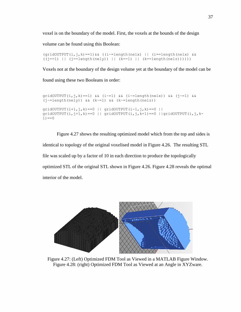
Example 3: Input Any STL File in this case an FDM tool
1. Enter optstl into the command window 2. When asked to input an STL, enter Y 3. When asked the STL filepath use FDMtool2.stl, for example C:\FDMtool2.stl.
FDMtool2.stl is scaled down for decreasing the number of elements and computation time.
4. When asked the height, enter 5 5. When asked the width, enter 11 6. When asked the depth, enter 16 7. When asked for a discretization factor, enter 3. You should get a MATLAB figure of
the voxelised model. 8. When asked for a load, enter P 9. When asked for the x-coordinate, enter 16 10. When asked for the y-coordinate, enter 14 11. When asked for the z-coordinate, enter 24 12. When asked for another load, enter N. 13. When asked for the load’s magnitude, enter -100 14. When asked for constraint, enter P 15. When asked for the x-coordinate, enter 0 16. When asked for the y-coordinate, enter 0 17. When asked for the z-coordinate, enter 0 18. When asked for another constraint, enter Y 19. When asked for constraint, enter P 20. When asked for the x-coordinate, enter 33 21. When asked for the y-coordinate, enter 0 22. When asked for the z-coordinate, enter 0 23. When asked for another constraint, enter Y 24. When asked for constraint, enter P 25. When asked for the x-coordinate, enter 33
77
26. When asked for the y-coordinate, enter 0 27. When asked for the z-coordinate, enter 48 28. When asked for another constraint, enter Y 29. When asked for constraint, enter P 30. When asked for the x-coordinate, enter 0 31. When asked for the y-coordinate, enter 0 32. When asked for the z-coordinate, enter 48 33. When asked for another constraint, enter N 34. When asked for the modulus, enter 2150 for ABS (e.g. 2150 MPa) . You should then
get an optimized model. 35. When asked to scale the model, enter N. 36. When asked respecting the boundary, enter Y. You should then get the optimized
model plus the boundary elements. 37. When asked to write an STL file, enter Y. 38. When asked for the file path, enter a full path for example C:\optFDMtool.st Original STL Topologically Optimized STL
79
Increasing Cantilever Discretization
Increasing platform discretization
Testing discretization and scaling of a 1 mm
3 unit cube
81
Figure H.1: The original cantilever’s plot for displacement in the X direction
Figure H.2: The original cantilever’s plot for displacement in the Y direction
Figure H.3: The original cantilever’s plot for displacement in the Z direction
82
Figure H.4: The original cantilever’s plot for resultant 3D strain
Figure H.5: The original cantilever’s plot for strain in the X direction
Figure H.6: The original cantilever’s plot for strain in the Y direction
83
Figure H.7: The original cantilever’s plot for strain in the Z direction
Figure K.8: The original platform’s plot for displacement in the X direction
84
Figure K.9: The original platform’s plot for displacement in the Y direction
Figure K.10: The original platform’s plot for displacement in the Z direction
Figure K.11: The original platform’s plot for resultant 3D strain
85
Figure K.12: The original cantilever’s plot for displacement in the X direction
Figure K.13: The original platofrm’s plot for displacement in the Y direction
88
Material Young's Modulus
(GPa) Density (g/cc)
Poisson’s Ratio
ABS 2.15 Gpa 1.07 0.3
Titanium Alloy
115 GPa 4.03 0.3
90
Mass for
Compress
ing
Prototype
Compress
ive force
(N)
height
(mm)
1st
Measure
ment
height
(mm)
2nd
Measure
ment
height
(mm)
3rd
Measure
ment
height
(mm)
Average
Std. Dev
(mm)
Prototype
's Strain
(ε)
Stress, PaControl
Strain (ε)
Design
Load
0 0 20.53 20.76 20.44 20.57667 0.165025 0 0 0 210420
10 44.49816 20.53 20.54 20.6 20.55667 0.037859 0.000972 93633.03 4.36E-05 210420
15 66.74724 20.58 20.51 20.56 20.55 0.036056 0.001296 140449.5 6.53E-05 210420
20 88.99632 20.54 20.52 20.57 20.54333 0.025166 0.00162 187266.1 8.71E-05 210420
25 111.2454 20.56 20.52 20.53 20.53667 0.020817 0.001944 234082.6 0.000109 210420
30 133.4945 20.52 20.52 20.53 20.52333 0.005774 0.002592 280899.1 0.000131 210420
40 177.9926 20.51 20.5 20.53 20.51333 0.015275 0.003078 374532.1 0.000174 210420
0
50000
100000
150000
200000
250000
300000
350000
400000
0 0.001 0.002 0.003 0.004
Stre
ss (
Pa)
Strain
Compression Test for ABS Prototype 1
E = 2.15 GPa
Prototype
Design Load
91
Mass for
Compress
ing
Prototype
Compress
ive force
(N)
height
(mm)
1st
Measure
ment
height
(mm)
2nd
Measure
ment
height
(mm)
3rd
Measure
ment
height
(mm)
Average
Std. Dev
(mm)
Prototype
's Strain
(ε)
Stress, PaControl
Strain (ε)
0 0 20 19.99 20.01 20 0.01 0 0 0
10 44.49816 19.99 19.98 19.99 19.98667 0.005774 0.000667 93633.03 4.36E-05
15 66.74724 19.98 19.99 19.98 19.98333 0.005774 0.000833 140449.5 6.53E-05
20 88.99632 19.96 19.98 19.98 19.97333 0.011547 0.001333 187266.1 8.71E-05
25 111.2454 19.97 19.97 19.97 19.97 0 0.0015 234082.6 0.000109
30 133.4945 19.95 19.96 19.97 19.96 0.01 0.002 280899.1 0.000131
40 177.9926 19.94 19.96 19.96 19.95333 0.011547 0.002333 374532.1 0.000174
0
50000
100000
150000
200000
250000
300000
350000
400000
0 0.0005 0.001 0.0015 0.002 0.0025
Stre
ss (
Pa)
Strain
Compression Test for ABS Prototype 2
E = 2.15 GPa
Prototype
Design Load
92
Mass for
Compress
ing
Prototype
Compress
ive force
(N)
height
(mm)
1st
Measure
ment
height
(mm)
2nd
Measure
ment
height
(mm)
3rd
Measure
ment
height
(mm)
Average
Std. Dev
(mm)
Prototype
's Strain
(ε)
Stress, PaControl
Strain (ε)
Design
Load
0 0 20 20.02 20.02 20.01333 0.011547 0 0 0 210420
10 44.49816 20.01 20.01 20 20.00667 0.005774 0.000333 93633.03 4.36E-05 210420
15 66.74724 20.01 20 20 20.00333 0.005774 0.0005 140449.5 6.53E-05 210420
20 88.99632 20.01 19.99 20 20 0.01 0.000666 187266.1 8.71E-05 210420
25 111.2454 19.99 19.99 19.99 19.99 0 0.001166 234082.6 0.000109 210420
30 133.4945 19.99 19.98 19.98 19.98333 0.005774 0.001499 280899.1 0.000131 210420
40 177.9926 19.97 19.98 19.97 19.97333 0.005774 0.001999 374532.1 0.000174 210420
0
50000
100000
150000
200000
250000
300000
350000
400000
0 0.0005 0.001 0.0015 0.002 0.0025
Stre
ss (
Pa)
Strain
Compression Test for ABS Prototype 3
E = 2.15 GPa
Prototype
Design Load
93
Mass for
Compressing
Prototype
Compress
ive force
(N)
height
(mm)
1st
Measure
ment
height
(mm)
2nd
Measure
ment
height
(mm)
3rd
Measure
ment
height
(mm)
Average
Std. Dev
(mm)
Prototype
's Strain
(ε)
Stress, PaControl
Strain (ε)
Design
Load
0 0 20 20 20 20 0 0 0 0 210420
10 44.49816 19.99 20 20 19.99667 0.005774 0.000167 93633.03 4.36E-05 210420
15 66.74724 20 19.98 19.99 19.99 0.01 0.0005 140449.5 6.53E-05 210420
20 88.99632 20 19.98 19.97 19.98333 0.015275 0.000833 187266.1 8.71E-05 210420
25 111.2454 19.99 19.98 19.97 19.98 0.01 0.001 234082.6 0.000109 210420
30 133.4945 19.98 19.97 19.96 19.97 0.01 0.0015 280899.1 0.000131 210420
40 177.9926 19.97 19.97 19.96 19.96667 0.005774 0.001667 374532.1 0.000174 210420
0
50000
100000
150000
200000
250000
300000
350000
400000
0 0.0005 0.001 0.0015 0.002 0.0025
Stre
ss (
Pa)
Strain
Compression Test for ABS Prototype 4
E = 2.15 GPa
Prototype
Design Load
94
Mass for
Compress
ing
Prototype
Compress
ive force
(N)
height
(mm)
1st
Measure
ment
height
(mm)
2nd
Measure
ment
height
(mm)
3rd
Measure
ment
height
(mm)
Average
Std. Dev
(mm)
Prototype
's Strain
(ε)
Stress, PaControl
Strain (ε)
Design
Load
0 0 19.99 20 20 19.99667 0.005774 0 0 0 210420
10 44.49816 19.99 19.98 19.99 19.98667 0.005774 0.0005 93633.03 4.36E-05 210420
15 66.74724 19.97 19.98 19.98 19.97667 0.005774 0.001 140449.5 6.53E-05 210420
20 88.99632 19.97 19.97 19.98 19.97333 0.005774 0.001167 187266.1 8.71E-05 210420
25 111.2454 19.97 19.96 19.96 19.96333 0.005774 0.001667 234082.6 0.000109 210420
30 133.4945 19.96 19.96 19.97 19.96333 0.005774 0.001667 280899.1 0.000131 210420
40 177.9926 19.95 19.95 19.96 19.95333 0.005774 0.002167 374532.1 0.000174 210420
0
50000
100000
150000
200000
250000
300000
350000
400000
0 0.0005 0.001 0.0015 0.002 0.0025
Stre
ss (
Pa)
Strain
Compression Test for ABS Prototype 5
E = 2.15 GPa
Prototype
Design Load
96
Cantilever loads and constraints
Load Location: point force at (x = 30 mm , y = 0 mm, and z = 0 mm)
Load Location: point force at (x = 30 mm , y = 0 mm, and z = 1 mm)
Load Location: point force at (x = 30 mm , y = 0 mm, and z = 2 mm)
Load magnitude = -100 N (program will distribute this load across the thre nodes above
which represent the tip of the cantilever, so each load is -33.333 N)
Simply Supported Constraints at x = 0 mm, 0 mm ≤ y ≤ 10 mm, and 0 mm ≤ z ≤ 2 mm
Platform loads and constraints
Load Location: point force at (x = 20 mm , y =20 mm, and z = 20 mm)
Simply Supported Constraints at (x=0mm, y = 0mm, z = 0mm), (x=40mm, y = 0mm, z =
0mm), (x=40 mm, y = 0 mm, z = 40 mm), and (x=0mm, y = 0mm, z =40 mm)
FDM Tool loads and constraints
Load Location: point force at (x = 15mm , y = 14 mm, and z = 24 mm)
Load Magnitude: -100N
Simply Supported Constraints at (x=0mm, y = 0mm, z = 0mm), (x=33mm, y = 0mm, z =
0mm), (x=33mm, y = 0mm, z = 48mm), and (x=0mm, y = 0mm, z =48 mm)
97
BIBLIOGRAPHY
[1] Amir, O., Aage, N., and Lazarov, B. S., 2014, “On multigrid-CG for
efficient topology optimization,” Structural and Multidisciplinary
Optimization, Vol 49, No.5, pp 815-829.
[2] Andreassen, E. and Andreasen, C. S., 2014, “How to determine composite
material properties using numerical homogenization,” Computational
Materials Science, Vol. 83, pp 488-495.
[3] Andreasen, C. S. and Sigmund, O., 2012, “Multiscale modeling and
topology optimization of poroelastic actuators,” Smart Materials and
Structures, Vol. 21, No. (6).
[4] Andreasen, C. S., Andreassen, E., Jensen, J. S., and Sigmund, O., 2014,
“On the realization of the bulk modulus bounds for two-phase viscoelastic
composites,” Journal of the Mechanics and Physics of Solids, Vol 63, pp
228-241.
[5] Digital Manufacturing & Design Innovation (DMDI) Institute, 2013,
“Awardee Announced”. US National Network for Manufacturing
Innovation. http://manufacturing.gov/dmdi.html. Last visited on 6/20/2014
[6] Banerjee, J., Chou, H. T., Garza, J. F., Kim, W., Woelk, D., Ballou, N.,
and Kim, H. J., 1987, “Data model issues for object-oriented
applications,” ACM Transactions on Information Systems (TOIS), Vol 5,
No. 1, pp 3-26.
[7] Bendsoe, M. P. and Sigmund, O. 2003. Topology optimization: theory,
methods and applications. Springer.
[8] Bereiter, C., 2002, “Design Research for Sustained Innovation”. Cognitive
Studies, Bulletin of the Japanese Cognitive Science Society. Vol 9. p 321
– 327.
[9] Brackett, D., Ashcroft, I., and Hague, R., 2011, “Topology optimization
for additive manufacturing,” In Proceedings of the 24th Solid Freeform
Fabrication Symposium (SFF11 ׳). pp. 6-8.
[10] Chu, J., Engelbrecht, S., Graf, G., and Rosen, D. W., 2010, “A comparison
of synthesis methods for cellular structures with application to additive
manufacturing,” Rapid Prototyping Journal, Vol. 16, No. 4, pp 275-283.
98
[11] Emmelmann, C., Sander, P., Kranz, J., & Wycisk, E. 2011. Laser additive
manufacturing and bionics: redefining lightweight design. Physics
Procedia, 12, pp 364-368.
[12] General Electric, 2014,“Transforming Manufacturing One Layer at a
Time”. Additive Manufacturing is Reinventing the Way We Work.
http://www.ge.com/stories/additive-manufacturing. Last visited
10/27/2014.
[13] Gere, J.M., Goodno, B.J., 2009, Mechanics of Materials, 7th
ed, pp 23-24.
[14] Gero, J. S. 1990. “Design prototypes: a knowledge representation schema
for design,” AI magazine, Vol. 11, No. 4, pp 26.
[15] National Science Foundation, 2014, “GOALI: Building Engineering
Through Topology Optimization”. National Science Foundation Where
Discoveries Begin.
http://www.nsf.gov/awardsearch/showAward?AWD_ID=1335160 . Last
visited on 6/20/2014.
[16] Hiller, J., and Lipson, H. 2009, “Design and analysis of digital materials
for physical 3D voxel printing,” Rapid Prototyping Journal, 15(2), pp
137-149.
[17] Kashdan, L., Seepersad, C. C., Haberman, M., and Wilson, P. S. 2012,
“Design, fabrication, and evaluation of negative stiffness elements using
SLS,” Rapid Prototyping Journal, 18(3), pp 194-200.
[18] Kiureghian, A. D. and Ditlevsen, O. 2009, “Aleatory or epistemic? Does it
matter?,” Structural Safety, 31(2), pp 105-112.
[19] Liu, K., and Tovar, A, 2014, “An efficient 3D topology optimization code
written in Matlab.” Structural and Multidisciplinary Optimization.
[20] Nguyen, T. H., Paulino, G. H., Song, J., and Le, C. H. 2010. A
computational paradigm for multiresolution topology optimization
(MTOP). Structural and Multidisciplinary Optimization, 41(4), pp 525-
539.
[21] Oded A., 2014, “Oded Amir”, http://tx.technion.ac.il/~odedamir/ , Last
visited on 6/20/2014.
99
[22] AM News, 2014 “Pitt Reserachers Receive America Makes Grant to
Develop Computational “Latticework” for Additive Manufacturing”.
Additive Manufacturing.
http://additivemanufacturing.com/2014/02/12/pitt-researchers-receive-
america-makes-grant-to-develop-computational-latticework-for-additive-
manufacturing/ , Last visited on 6/20/2014.
[23] Ruffo, M., Tuck, C., and Hague, R. 2006. Cost estimation for rapid
manufacturing-laser sintering production for low to medium volumes.
Proceedings of the Institution of Mechanical Engineers, Part B: Journal
of Engineering Manufacture, 220(9), pp 1417-1427.
[24] Taminger, K. M., and Hafley, R. A. 2003. Electron beam freeform
fabrication: a rapid metal deposition process. In Proceedings of the 3rd
Annual Automotive Composites Conference, pp. 9-10.
[25] Tomlin, M. and Meyer, J. 2011. Topology optimization of an additive
layer manufactured (ALM) aerospace part. In The 7th Altair CAE
Technology Conference, Gaydon, UK, 10th May.
[26] Wang, H. V., & Rosen, D. W. 2001. Computer-aided design methods for
the additive fabrication of truss structure (Master's thesis, School of
Mechanical Engineering, Georgia Institute of Technology).
100
VITA
Purnajyoti Bhaumik is 28 year old full time Mechanical Project Engineer for
Vanderlande Industries. He has 2.5 years of experience as an engineer and served in the
United States Marine Corps Reserve for 6 years. He has a Bachelor of Science degree in
Mechanical Engineering from the Georgia Institute of Technology, an Engineer
Intern/Engineer in Training Certificate in Mechanical Engineering, a Lean Six Sigma Black
Belt, and a Graduate Certificate in CAD/CAM and Rapid Prototyping.
He started school at the Missouri University of Science and Technology in the Fall of
2012. He completed my graduate certificate work in the Spring of 2013 with a 3.25 GPA. He
decided to try the Master of Science in Mechanical Engineering degree program and
maintained a 3.28 GPA. He studied state space controls, optimization, DFMA, solid freeform
modeling, solid freeform fabrication, and FEA.
He shall begin studying for his PE exam in 2015. At work, he shall be responsible for
optimizing engineering design specifications based on functional requirements, quality, cost,
and time. He shall look forward to traveling and visiting my extended family across the
globe. He shall consider undertaking a PhD in Mechanical Engineering.