Globalization Institute Working Paper 372 Research Department https://doi.org/10.24149/gwp372 Working papers from the Federal Reserve Bank of Dallas are preliminary drafts circulated for professional comment. The views in this paper are those of the authors and do not necessarily reflect the views of the Federal Reserve Bank of Dallas or the Federal Reserve System. Any errors or omissions are the responsibility of the authors. Generational War on Inflation: Optimal Inflation Rates for the Young and the Old Ippei Fujiwara, Shunsuke Hori and Yuichiro Waki
Transcript
Globalization Institute Working Paper 372 Research Department https://doi.org/10.24149/gwp372
Working papers from the Federal Reserve Bank of Dallas are preliminary drafts circulated for professional comment. The views in this paper are those of the authors and do not necessarily reflect the views of the Federal Reserve Bank of Dallas or the Federal Reserve System. Any errors or omissions are the responsibility of the authors.
Generational War on Inflation: Optimal Inflation Rates for the
Generational War on Inflation: Optimal Inflation Rates for the Young and the Old*
Ippei Fujiwara†, Shunsuke Hori‡ and Yuichiro Waki§
October 27, 2019
Abstract How does a grayer society affect the political decision-making regarding inflation rates? Is deflation preferred as a society ages? In order to answer these questions, we compute the optimal inflation rates for the young and the old respectively, and explore how they change with demographic factors, by using a New Keynesian model with overlapping generations. According to our simulation results, there indeed exists a tension between the young and the old on the optimal inflation rates, with the optimal inflation rates differing between generations. The rates can be significantly different from zero, particularly, when heterogeneous impacts from inflation via nominal asset holdings are considered. The optimal inflation rates for the old can be largely negative, reflecting their positive nominal asset holdings as well as lower effective discount factor. Societal aging may exert downward pressure on inflation rates through a politico-economic mechanism. Keywords: Optimal inflation rates; Societal aging; Heterogeneous agents JEL codes: E31; E52; J11
*We have benefited from discussions with Simon Alder, Dongchul Cho, Dave Cook, Chris Edmond, Greg Kaplan, Jinill Kim, Bob King, Antoine Lepetit, Thomas Lubik, Toan Phan, Bruce Preston, Stan Rabinovich, Andrew Rose, Alex Wolman, Jenny Xu, Makoto Yano, and the conference and seminar participants at FRB Richmond, Hong Kong University of Science and Technology, NBER–EASE, the Research Institute of Economy, Trade and Industry (RIETI), University of Melbourne and University of North Carolina at Chapel Hill. This study is conducted as a part of the project “Monetary and fiscal policy in the low growth era” undertaken at RIETI. Fujiwara is also grateful for financial support from JSPS KAKENHI Grant-in-Aid for Scientific Research (A) Grant Number 15H01939 and 18H036038. The views in this paper are those of the authors and do not necessarily reflect the views of the Federal Reserve Bank of Dallas or the Federal Reserve System. Any errors or omissions are the responsibility of the authors. †Ippei Fujiwara, Keio University, The Australian National University and ABFER, [email protected]. ‡Shunsuke Hori, University of California, San Diego, [email protected]. §Yuichiro Waki, Aoyama Gakuin University, [email protected].
Japan has experienced long-lasting deflation or low inflation rates for more than two
decades. Some claim that this is due to the failure of monetary policy, with insufficient
reaction by the Bank of Japan to declining aggregate demand, based on the idea that
“[i]nflation is always and everywhere a monetary phenomenon,” by Friedman (1963).
On the other hand, because of its long-lasting nature, others point out that chronic
deflation or disinflation should have its root in structural issues. An interesting ob-
servation about the relationship between structural factors and nominal developments
in Japan is that deflation or disinflation started around the mid-1990s, which is also
when the working age population also started decreasing. Is it a causal relationship
or merely coincidence? This paper offers a new insight on the possible structural rela-
tionship between deflation and aging by examining whether the optimal inflation rates
differ between the young and the old.
An aging population and low inflation rates are not phenomena intrinsic only to
Japan and are now observed in many developed economies, leading several researchers
to investigate the possible causal relationship between inflation dynamics and demo-
graphic changes. Carvalho and Ferrero (2014) and Fujita and Fujiwara (2016) discuss
how societal aging can lead to the declining natural rate of interest, which naturally ex-
erts downward pressure on inflation rates with insufficient monetary policy responses.
Carvalho and Ferrero (2014) focus on the demand channel, or consumption-saving het-
erogeneity. Longer longevity induces higher saving rates for self-insurance. Such a
saving-for-retirement motive can account for roughly 30% to 50% of the decline in real
interest rates in Japan. The decline in fertility rate, however, does not have large im-
pacts. On the other hand, Fujita and Fujiwara (2016) quantify the impact of the supply
channel, or skill (productivity) heterogeneity. The changes in the demographic structure
induce significant low-frequency movements in per-capita consumption growth and
the real interest rate through changes in the composition of skilled (old) and unskilled
(young) workers. This mechanism can account for roughly 40% of the decline in the
real interest rate observed between the 1980s and 2000s in Japan. The key is the declin-
ing fertility (labor participation) rate.
Doepke and Schneider (2006) explore the redistribution effect of inflation. Since
the old own more nominal financial assets, they are more vulnerable to unanticipated
inflation. On the other hand, surprise inflation can be beneficial to the young as they
are borrowers with nominal debt contracts. This conclusion obtained by Doepke and
Schneider (2006) also hints that social preference for inflation or deflation may depend
2
on the demographic structure.1
We also inquire into whether there is a structural relationship between demographic
changes and inflation dynamics, but with a different angle. In particular, we com-
pute the optimal inflation rates in the spirit of Schmitt-Grohe and Uribe (2010) with a
politico-economic consideration following Bassetto (2008), who studies the inter-generational
conflicts in tax policy in overlapping generations. Previous studies focus on how infla-
tion or a nominal shock affects heterogeneous agents differently. Instead, we explore
how the optimal inflation rates differ between the young and the old, given the hetero-
geneous impacts of monetary policy.2 There are many studies pointing out the hetero-
geneous impacts of monetary policy - Fujiwara and Teranishi (2008), Gornemann et al.
(2016), Kaplan et al. (2018), Debortoli and Galí (2017), Wong (2016) and Eichenbaum
et al. (2018). To the best of our knowledge, however, ours is the first study to compute
the optimal inflation rates for heterogeneous agents.
As comprehensively analyzed in Schmitt-Grohe and Uribe (2010), specifically for
Calvo (1983) contract in Ascari (2004) and for Rotemberg (1982) adjustment costs in
Bilbiie et al. (2014), inflation rates are not neutral even in (stochastic) steady states. In-
flation rates affect mark-ups in the long-run through such nominal rigidities and have
impacts on real variables. As a result, optimal inflation rates can be positive or nega-
tive depending on the deep parameters. Since the structural parameters differentiate
the behavior of the young and the old, the optimal inflation rates are likely to be dif-
ferent between these two agents.3 In addition, as implied by Doepke and Schneider
(2006) and Auclert (2017), the existence of nominal contracts in the financial transac-
tions will lead to asymmetric preference for inflation rates by young and old agents,
given the heterogeneity in their nominal asset positions.
We compute the optimal inflation rates for the young and the old, and also how
they change with different demographic demographic settings. For this purpose, we
employ the overlapping generations model with nominal rigidities by Fujiwara and
Teranishi (2008), where there are two consumers: the young and the old. They are
1Auclert (2017) classifies three channels where monetary policy, namely, a surprise nominal shock,causes redistribution: an earning heterogeneity channel; a Fisher channel; and an interest rate exposure chan-nel. Auclert (2017) finds that all three channels amplify the effects of monetary policy. From a normativeperspective, Sheedy (2014) shows that nominal GDP targeting is desirable in an economy with nominalfinancial contracts, since it can improve risk sharing.
2In this regard, our paper’s aim is similar to that in Bullard et al. (2012). They construct an over-lapping generations model with two assets - capital and money. If old agents have more influenceon political decision making, relatively low inflation is chosen because lower inflation reduces the op-portunity cost of holding money and money becomes relatively more attractive, thus reducing capitalaccumulation. This raises interest rates, which is preferred by the old since they rely more on capitalincome than labor income.
3This is indeed due to the earnings heterogeneity channel coined by Auclert (2017) in terms of infla-tion rates.
3
different in life expectancy and the labor productivity. Unlike the standard overlap-
ping generations model, the transition from the young to the old follows a Markov
process with the latter being the absorbing state.4 Consequently, without resorting to
highly numerical analysis dealing with a large number of, say generations (50 years x
4 quarters = 200 generations), the analysis over the quarterly frequency, where mon-
etary policy is considered to be effective, becomes possible in a tractable framework.
In addition, aggregate dynamics as well as each group’s utilitalian welfare depend
on the wealth distribution only through two numbers: the within-group aggregate
wealth for the young and the old. Thanks to the assumption of RINCE preferences a
la Farmer (1990), within each age group, both the decision rule and the value function
have closed form solutions and they are linear in wealth. We can thus define the op-
timal inflation rates as those maximizing these values. These altogether enable us to
understand the mechanisms behind non-zero optimal inflation rates for heterogeneous
agents more intuitively, which is the main aim of this paper.
These are almost equivalent to the optimal steady state inflation rates. Any changes in
inflation rates, however, alter real variables in the steady state including endogenous
state variables in an economy with heterogeneous agents. In such a model, to allow
for the proper comparison of welfare at different inflation rates so that we can compute
the optimal inflation rates, welfare given the same initial values for the state variables
becomes the metric to be used. Thus, we call these optimal inflation rates in the long-
run instead of the optimal steady state inflation rates in this paper.5
The optimal inflation rates in the long-run are different both from zero and between
the young and the old, implying the importance of demographic factors in determining
the target level of inflation. The demographic structure not only determines the level
of the optimal inflation rates, but also changes the signs of the optimal inflation rates
for the young and the old.
We show that the slope of the steady state Phillips curve, namely whether inflation in-
creases or reduces mark-ups in the steady state, depends on the size of the steady state
interest rates, particularly whether they are higher or lower than the potential growth
rate. Changes in the demographic structure naturally lead to the different steady state
interest rates. For example, longer life expectancy causes a stronger motive for saving-
for-retirement, which lowers steady state interest rates. As a result, the slope of the
eficial to the old since this reduces marginal costs and therefore increases mark-ups.
4The overlapping generations model by Gertler (1999) can be considered as the generalizedBlanchard-Rarity model a la Blanchard (1985) and Yaari (1965).
5The differences in the initial values of endogenous state variables, however, only leads to marginaldifferences in the optimal inflation rates.
4
The opposite effects occur when the interest rates are higher than the potential growth
rate in the steady state. To the best of our knowledge, this is the first study to investi-
gate this non-trivial relationship between the optimal inflation rates and demographic
factors in the long-run.
The optimal inflation rates in the long-run are, however, only marginally differ-
ent from zero. When analyzing the optimal inflation rates for the young and the old
in the long-run, we deliberately abstract heterogeneous impacts from surprise infla-
tion via nominal asset holdings. If these are considered, the optimal inflation rates for
the young and the old can be considerably non-zero from the re-distributional motive
through the Fisher channel.
We compute the optimal inflation rates for the young and the old given nominal
financial contracts. In an economy with nominal contracts, changes in the target level
inflation affect debtors and creditors differently. The central bank needs to set the target
level of inflation to take the right balance between short-run gains (or losses) for some
particular agents and long-run gains from price stability for all agents. If the former is
substantial to some agent, the optimal inflation rate for this agent must be significantly
different from zero.
The heterogeneous impacts from surprise inflation via nominal asset holdings turn
out to be large. As a result, the optimal inflation rates for old agents, who are net nom-
inal creditors, become largely negative ranging from -0.7% to -5.5% under reasonable
parameter calibration. With an increasing number of elderly people, societal aging may
exert downward pressure on inflation rates through a politico-economic mechanism.6
Naturally, the optimal inflation rates for the young are positive under reasonable
parameter calibration, yet they are not significantly different from zero, showing a
stark contrast to those for old agents, whose optimal inflation rates are significantly
negative. Why is there such a large asymmetry in the optimal inflation rates between
the young and the old? To understand the reason behind this asymmetry, we examine
which heterogeneity matters for this stark contrast. We first eliminate the heterogeneity
in labor productivity and then in the effective discount factor.
We find that the effective discount factor, namely, life expectancy, is key to this
asymmetry. Even without heterogeneity in labor productivity, this stark contrast some-
what remains. On the other hand, when all agents become almost immortal, the opti-
mal inflation rates for the old become very close to zero, similarly to those for young
agents. With the presence of the survival rate, old agents become myopic. Benefits
6Katagiri et al. (2019) explains the negative correlation between inflation and aging from a politico-economic perspective. The key mechanism in their paper is the FTPL (Fiscal Theory of the Price Level)and the changes in the tax base via aging. On the other hand, ours is to seek the optimal inflation ratesunder monetary dominance.
5
from setting non-zero inflation targets stem from the redistribution via nominal con-
tracts. Therefore, they are considered short-run gains. On the other hand, costs are
price adjustment costs or price dispersion, which persist as long as inflation rates are
not zero. Therefore, they are long-run losses. As life expectancy increases (the survival
rate becomes higher), old agents become more like young agents and the long-run
costs from non-zero inflation rates get larger. Consequently, the optimal inflation rates
for old agents become closer to zero even though they lend to the young with nominal
fixed contracts.
The remainder of the paper is structured as follows. Section 2 describes the model
used in this paper. In Section 3, we show how the optimal inflation rates are different
between the young and the old and how they change by different demographic struc-
ture. Section 4 incorporates nominal financial contracts and explore their implications
on the optimal inflation rates for the young and the old. Section 5 concludes.
2 The Model
In order to investigate the effects of societal aging on the optimal inflation rate, we em-
ploy the overlapping generations (OLG) model used in Fujiwara and Teranishi (2008)
that extends the analytical framework in Gertler (1999) to incorporate nominal rigidi-
ties and monetary policy. Unlike the standard overlapping generations model, the
transition from the young to the old follows a Markov process with the latter being the
absorbing state. This enables us to understand the mechanisms behind non-zero opti-
mal inflation rates for heterogeneous agents more intuitively in a tractable framework.
We also assume perfect foresight throughout all analyses in this paper.
There are six agents in this model economy: two types of consumers - the young
and the old; final good producers; intermediate goods producers; a capital producer
(financial intermediary); and the central bank. The problems which each of the agents
except for the central bank faces are as follows.7 The central bank sets inflation rate in
order to maximize welfare.
2.1 Consumers
Each young agent faces a constant probability ω to become old, while each old agent
remains in the population with the survival probability γ. Each type of agent is also
different in labor productivity. In the benchmark model, only young agents supply one
unit of labor. To be precise, we set old agents’ relative labor productivity ξ to be zero.
7For details of the derivation, see Gertler (1999) and Fujiwara and Teranishi (2008).
6
As a result, old agents receive no labor compensation and never work. Appendix A
shows the model with endogenous adjustments in intensive margin with non-zero ξ.
Young and old agents are heterogeneous in the effective discount factor and labor
productivity. As a result, the marginal propensities to consume become different be-
tween them, leading to heterogeneous impacts of monetary policy. Also, agents are
heterogeneous in asset positions since each agent was born and retired at a different
point in time. The heterogeneity in asset positions does not, however, matter for aggre-
gation over young and old agents, respectively. Our model assumes RINCE (RIsk Neu-
trality and Constant Elasticity of Substitution) preferences proposed by Farmer (1990),
which is a special case of the Epstein and Zin (1989) preference with risk neutrality.
With RINCE preferences, consumption function becomes linear in wealth. Thus, only
the aggregate wealth matters for aggregate consumption of both young and old agents.
RINCE preferences also allow us to derive the closed form solutions for value func-
tions of agents who are either young or old at any arbitrary time t. We can thus define
the optimal inflation rates as those maximize these values. These altogether enable us
to understand the mechanisms behind non-zero optimal inflation rates for heteroge-
neous agents more intuitively.
There is a perfect annuity market. Therefore, old agents do not face any income un-
certainty and enjoy the same ex post rate of return as young agents. On the other hand,
there is no insurance market for aging risk. In this regard, markets are incomplete in
this model.
Let us first discuss the optimization problem of the old, which is assumed to be the
absorbing state.
2.1.1 Old
At time t, an old agent, denoted by superscript o, who was born at period j and became
old at period k, maximizes the lifetime utility:
Voj,k,t :=
{(Co
j,k,t
)ρ+ βγ
(Vo
j,k,t+1
)ρ} 1ρ
,
subject to the budget constraint:
Aoj,k,t
Pt=
Rt−1
γ
Aoj,k,t−1
Pt− Co
j,k,t + Doj,k,t.
Ct, At, Pt, and Rt denote consumption, financial assets, aggregate price, and nominal
interest, respectively. The old do not supply labor. Dt is the sum of the transfer (or
tax) from the government and profits rebated from producers by the ownership of
7
these firms. β and ρ define the common subjective discount factor for both the young
and the old, and the inverse of the intertemporal elasticity of substitution, respectively.
The next period welfare is discounted by βγ since the old must take the survival rate
into account in maximizing welfare. The rate of return from holding financial assets
is divided by γ because of the perfect annuity market among old agents. As a result,
bequests are distributed equally among surviving old agents.8
2.1.2 Young
A young agent, denoted by the superscript y, who was born at period j maximizes the
life time utility:
Vyj,t :=
{(Cy
j,t
)ρ+ β
[ωVy
j,t+1 + (1−ω)Voj,t+1
]ρ} 1ρ
,
subject to the budget constraint
Ayj,t
Pt= Rt
Ayj,t−1
Pt+
Wt
Pt− Cy
j,t + Dyj,t.
Since each young agent becomes old with probability ω, the next period value is
weighted value of the young and the old. In contrast to the old, the young supply
one unit of labor and obtain nominal wage Wt.
2.2 Firms
Final goods, Yt, are produced by the final goods producers in a competitive market.
Differentiated intermediary goods are aggregated by the production technology:
Yt :=[∫ 1
0(Yi,t)
κ−1κ di
] κκ−1
.
The parameter κ denotes the elasticity of substitution among differentiated intermedi-
ate goods. Given the aggregate price level Pt and the price of each intermediary goods
Pi,t, profit maximization by the final good firm yields the demand for each intermediate
good:
Yi,t =
(Pi,t
Pt
)−κ
Yt. (1)
Firm i in a monopolistically competitive market uses non-differentiated labor Li,t
and capital Ki,t−1 in order to produce differentiated intermediate goods Yi,t. The pro-
8More explicit modeling for the annuity market and the ownership of firms through equity holdingsis possible. This will not, however, change our results since perfect foresight is assumed in this paper.
8
duction function of the intermediate goods is given by
Yi,t := L1−αi,t Kα
i,t−1, (2)
where α is capital share. Labor is supplied by consumers with nominal wage rate Wt.
Capital is rented to intermediary firms at real rate RKt from the capital producer. The
real cost minimization problem is thus given by
min(
Wt
PtLi,t + rK
t Ki,t−1
)subject to the production function (2). This gives the optimal factor price conditions:
Wt
Pt= (1− α)ψt (Li,t)
−α Kαi,t−1,
rKt = αψtL1−α
i,t Kα−1i,t−1,
where ψt denotes real marginal costs.
Since each intermediary firm is in a monopolistically competitive market, it chooses
price to maximize the profit subject to the Rotemberg (1982) price adjustment costs
with the cost parameter φ. Instantaneous real profit ΠIi,t is given by
ΠIi,t := (1 + τ)
Pi,t
PtYi,t − ψtYi,t −
φ
2
(Pi,t
Pi,t−1− 1)2
Yt.
We assume that the intermediaries are owned by consumers and therefore, the profit
is rebated equally to all consumers. Let m0,t denote the pricing kernel. Then, the profit
maximization problem by price setting becomes
max∞
∑t=0
m0,tΠIi,t,
subject to the demand for intermediary goods in equation (1).
Since there are heterogeneous agents, defining the pricing kernel is not trivial.9 In
this paper, following Ghironi (2008) and Fujiwara and Teranishi (2008), we only con-
duct perfect foresight simulations, and therefore all assets yield same rates of return
among different agents both ex ante and ex post. In other words, the profit is discounted
by the risk free rate. This assumption, however, only matters in the initial period when
the target level of inflation is altered.
In order to eliminate the steady state distortion stemming from monopolistic com-
9For the detailed discussion on this issue, see Carceles-Poveda and Coen-Pirani (2009).
9
petition, production subsidy τ = 1κ−1 is assumed. This subsidy is financed by the lump
sum tax to both types of consumers.10
2.2.1 Calvo Pricing
We also examine the case with Calvo (1983) pricing. In this case, intermediate goods
producer i maximizes
max∞
∑t=0
λtm0,t
[(1 + τ)
Pi,t
PtYi,t − ψtYi,t
],
subject again to the downward sloping demand curve in equation (1). λ denotes the
Calvo (1983) parameter. Intermediate goods firms can reset the price with uncondi-
tional probability of 1− λ. The model with Calvo (1983) pricing is shown in Appendix
B.
2.3 Capital Producer
A capital producer maximizes the profit:
∞
∑t=0
m0,tΠKt ,
where the instantaneous profit is given by
ΠKt :=
At
Pt− Rt
At−1
Pt+ rK
t Kt−1 − It,
subject to the capital producing technology:
Kt = (1− δ)Kt−1 +
[1− S
(It
It−1
)]It.
A capital producer issues financial asset At with nominal rate of return Rt. Such fund-
ing from households and the receipts from renting the capital to the intermediate goods
producer are allocated to the repayment of borrowing from households and invest-
ment It. S (·) denotes the investment growth adjustment costs used in Christiano et al.
(2005):
S (xt) := s(
x2t
2− xt +
12
).
This capital producer can be also interpreted as a financial intermediary.
10Note that even the lump sum tax is not neutral under heterogeneous consumers.
10
2.4 Aggregate Conditions
The financial market clears with
qtKt =At
Pt,
and
At = Ayt + Ao
t ,
where Ayt = ∑∞
j=0 Ayj,t and Ao
t = ∑∞j=0 ∑∞
k=0 Aoj,k,t. qt denotes Tobin’s Q, which is given
by the Lagrange multiplier on the constraint in the capital producer’s profit maximiza-
tion problem.
The good market clears as
Yt = Ct + It +φ
2(πt − 1)2 Yt,
where Ct = Cyt + Co
t , Cyt = ∑∞
j=0 Cyj,t and Co
t = ∑∞j=0 ∑∞
k=0 Coj,k,t.
We deliberately assume that the profits are distributed by the relative asset hold-
ings:
Dot =
∞
∑j=0
∞
∑k=0
Doj,k,t =
Aot−1
Ayt−1 + Ao
t−1Dt, (3)
and
Dyt =
∞
∑j=0
Dyj,t =
Ayt−1
Ayt−1 + Ao
t−1Dt, (4)
where
Dt := ΠIt + ΠK
t − τYt =
[1− ψt −
φ
2(π − 1)2
]Yt +
At
Pt− Rt
At−1
Pt+ rK
t Kt−1 − It − τYt,
under a symmetric equilibrium. This assumption eliminates re-distributional impacts
from inflation stemming from nominal financial contracts. We will first explore the op-
timal inflation rates in the long-run which are not subject to nominal financial contracts
in Section 3 and then incorporate re-distributional channel in Section 4.
The labor market clearing condition is given by
Lt := ∑i
Li,t = Nyt ,
where Nyt is the population of young workers at time t.
11
2.5 Equilibrium Conditions
2.5.1 Population
Let Not denote the population of old agents at period t. Then, the population dynamics
for the young and the old are, respectively, given by
Nyt+1 = bNy
t + ωNyt ,
and
Not+1 = γNo
t + (1−ω) Nyt ,
where b denotes the birth rate. The growth rate of (young) population n is given by
n := b + ω− 1.
Given these laws of motion, the ratio of the number of old over that of young agents,
denoted by Γt, evolves as
Γt+1 :=No
t+1
Nyt+1
=γNo
t + (1−ω) Nyt
bNyt + ωNy
t=
γ
b + ωΓt +
1−ω
b + ω.
At the stationary population, the ratio of the number of old over that of young agents
remain constant:
Γ =1−ω
b + ω− γ.
2.5.2 Equilibrium Conditions in a Monopolistically Competitive Market
From the first order necessary conditions of the above optimization problems, we have
the equilibrium conditions under a monopolistically competitive market. All grow-
ing variables are de-trended by Nyt . De-trended variables are denoted by lower case
characters. The system of equations except for the monetary policy rule is given by
where for simplicity of analysis, we define an auxiliary variable:
Φt := ω + (1−ω) ερ−1
ρ
t .
πt denotes gross inflation rates:
πt :=Pt
Pt−1.
θt and εtθt denote the marginal propensity to consume for the young and the old,
respectively. Θyt and Θo
t denote the aggregated human and financial wealth for the
young and the old. These equations together with monetary policy, which aims to
maximize welfare, determines the equilibrium.
Discussion: Surprise Inflation When the optimal long-run inflation rates are an-
alyzed, our model abstracts the effects of surprise inflation on different consumers
through nominal asset holdings analyzed in Doepke and Schneider (2006). The solved-
out consumption functions in equations (7) and (8) are expressed as the product of the
marginal propensity to consume and the wealth, which includes initial nominal assets
divided by the price level at time t. A jump in the price level or inflation seems to affect
the wealth of the young and the old differently.
If equations (5) and (9), which determine the profit and the financial wealth for the
old respectively, are substituted in equation (7), the solved-out consumption function
for the old collapses to
cot = εtθt{
aot−1
ayt−1 + ao
t−1
{[1− ψt −
φ
2(πt − 1)2
]yt +
ayt + ao
tPt
+rK
t1 + n
kt−1 − it − τyt
}+
γπt+1
(1 + n) RtΘo
t+1}. (11)
The initial real asset position, which is the nominal asset position divided by the price
level aot−1/Pt, disappears from the wealth. Thus, surprise inflation does not alter the
initial real asset position. This irrelevance result stems from our assumption that the
profits are shared by the same asset ratio for good producers as well as the capital
producer (financial intermediary) in equations (3) and (4), and that all financial assets
are identical. We relax this assumption later in Section 4.
14
2.5.3 Aggregate Value
We can obtain aggregated (de-trended) values for the young and the old at time t as
indirect utility:
vyt = (θt)
− 1ρ cy
t , (12)
and
vot = (εtθt)
− 1ρ co
t . (13)
These are the targets for the central bank to maximize. To be precise, we suppose a
situation where there are two political parties - the young party and the old party.
The young (old) party represents young (old) consumers at time t and insists that the
central banks commit to monetary policy that maximizes vyt (vo
t ).
The assumption of RINCE preferences a la Farmer (1990) enables us to derive the
closed form solutions for value of agents who are either young or old at any arbitrary
time t. This greatly simplifies the analysis in this paper and contributes to offering a
more intuitive explanation of the non-zero optimal inflation rates.
2.5.4 Monetary Policy
The central bank is equipped with a commitment technology that aims to maximize
welfare defined in equations (12) or (13). Welfare is evaluated at the beginning of tran-
sition from the initial state to the one with the new steady state inflation rate:
v0 = f (X−1, π̄) ,
where Xt denotes the vector of endogenous state variables and π̄ is the target level of
inflation rate. In a new state, the central bank follows the monetary policy rule:
πt = π̄,
and we investigate which π̄ attains the highest welfare.
Throughout the analyses in this paper, initial states are given by those under zero
inflation steady state. As shown in Bilbiie et al. (2014), differences in the initial state
variables can lead to incorrect welfare evaluation. The same initial state variables are
assumed when comparing welfare.11
11The optimal inflation rate found in this way depends on the initial state variables. However, even ifwe set initial state as steady state of ±5% inflation rate, the change is small and our main message stillholds.
15
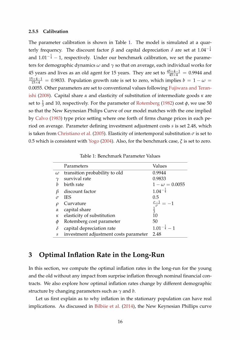
2.5.5 Calibration
The parameter calibration is shown in Table 1. The model is simulated at a quar-
terly frequency. The discount factor β and capital depreciation δ are set at 1.04−14
and 1.01−14 − 1, respectively. Under our benchmark calibration, we set the parame-
ters for demographic dynamics ω and γ so that on average, each individual works for
45 years and lives as an old agent for 15 years. They are set to 45×4−145×4 = 0.9944 and
15×4−115×4 = 0.9833. Population growth rate is set to zero, which implies b = 1− ω =
0.0055. Other parameters are set to conventional values following Fujiwara and Teran-
ishi (2008). Capital share α and elasticity of substitution of intermediate goods κ are
set to 13 and 10, respectively. For the parameter of Rotemberg (1982) cost φ, we use 50
so that the New Keynesian Philips Curve of our model matches with the one implied
by Calvo (1983) type price setting where one forth of firms change prices in each pe-
riod on average. Parameter defining investment adjustment costs s is set 2.48, which
is taken from Christiano et al. (2005). Elasticity of intertemporal substitution σ is set to
0.5 which is consistent with Yogo (2004). Also, for the benchmark case, ξ is set to zero.
Table 1: Benchmark Parameter Values
Parameters Valuesω transition probability to old 0.9944γ survival rate 0.9833b birth rate 1−ω = 0.0055β discount factor 1.04−
14
σ IES 0.5ρ Curvature σ−1
σ = −1α capital share 1
3κ elasticity of substitution 10φ Rotemberg cost parameter 50δ capital depreciation rate 1.01−
14 − 1
s investment adjustment costs parameter 2.48
3 Optimal Inflation Rate in the Long-Run
In this section, we compute the optimal inflation rates in the long-run for the young
and the old without any impact from surprise inflation through nominal financial con-
tracts. We also explore how optimal inflation rates change by different demographic
structure by changing parameters such as γ and b.
Let us first explain as to why inflation in the stationary population can have real
implications. As discussed in Bilbiie et al. (2014), the New Keynesian Phillips curve
16
-4 -3 -2 -1 0 1 2 3 4
Annual inflation rate (%)
0.997
0.9975
0.998
0.9985
0.999
0.9995
1
1.0005
1.001
1.0015
1.002
Ma
rgin
al co
st
Nominal interest rate = 4%
Nominal interest rate = 2%
Nominal interest rate = 0%
Nominal interest rate = -2%
Nominal interest rate = -4%
Figure 1: Steady state relationship with Rotemberg
in equation (6) implies that a fall in inflation rates raises marginal costs when interest
rates are low, while a rise in inflation rates raises marginal costs when interest rates are
high. To highlight this relationship, consider the New Keynesian Phillips curve in the
steady state:
ψ =κ + φπ
[−π2
R (1 + n) + πR (1 + n) + π − 1
]κ
.
Taking the derivative of the right hand side with respect to π gives
φ
[−3 π2
R (1 + n) + 2πR (1 + n) + 1
]κ
∣∣∣∣∣∣π=1
= φ
[− 1
R (1 + n) + 1]
κ,
which is positive when R > 1 + n. Namely, in the steady state, marginal costs rise as
inflation increases if and only if nominal interest is larger than the population growth
rate. Figure 1 shows the relationship between inflation rates and marginal costs can be
upward or downward sloping depending on the level of the steady state real interest
rate.
One may cast doubts on the existence of the long-run Phillips curve. Indeed, Benati
(2015) shows that there is no clear evidence of a non-vertical trade-off. Benati (2015),
however, also points out that uncertainty surrounding the estimates is substantial and
therefore, having priors about a reasonable slope in the long-run Phillips curve cannot
be falsified.
Intuition behind this long-run Phillips curve with Rotemberg adjustment costs is
17
-4 -3 -2 -1 0 1 2 3 4
Annual inflation rate (%)
0.99
0.992
0.994
0.996
0.998
1
1.002
Ma
rgin
al co
st
Nominal interest rate = 4%
Nominal interest rate = 2%
Nominal interest rate = 0%
Nominal interest rate = -2%
Nominal interest rate = -4%
Figure 2: Steady state relationship with Calvo
offered by Lepetit (2017): “Since adjusting prices is costly, firms do not pass on the
entirety of movements in marginal costs to prices and current inflation is associated
with a reduction in markups. ... [E]xpected future inflation leads firms to set higher
markups in order to minimize future price adjustments costs. However, these effects
are asymmetric. Since firms discount the future, higher inflation in t has a larger
positive impact on marginal cost at time t than a negative impact at time t − 1. In
other words, the model features a positive long-run relationship between inflation and
marginal cost.” Figure 2 illustrates that similar but slightly different long-run relation-
ship can be observed even with Calvo pricing.
Changes in marginal costs affect the young and the old differently. Figure 3 illus-
trates how inflation rates and other macroeconomic variables are related in the steady
states. Higher marginal costs raise real wages and interest rates. Increase in wages will
be welfare-enhancing for young agents as labor compensation is their main source of
income. On the other hand, low marginal costs increase welfare for the old because
low marginal costs increase firm profits. Since the old have two sources of income -
return from financial assets and profits from the ownership of firms - the strength of
this channel depends on the amount of asset holdings. Thus, inflation rates in the sta-
tionary population matters for relative welfare between the young and the old through
earning heterogeneity.
In order to understand how demographic changes affect optimal inflation rates for
both the young and the old, respectively, we examine how changes in life expectancy,
the population growth rate, the relative population, and the relative asset holdings
18
-0.01 0 0.01
Quartely inflation (%)
0.999996
0.999998
1
1.000002
1.000004Real marginal cost
-0.01 0 0.01
Quartely inflation (%)
2.63214
2.632145
2.63215
2.632155
2.63216
3.193354
3.193356
3.193358
3.19336
3.193362Real Wage
-0.01 0 0.01
Quartely inflation (%)
-0.281837
-0.2818369
-0.2818368
-0.2818367
-0.2818366
-0.96557
-0.965569
-0.965568
-0.965567
-0.965566(Net) Real interest rate (%)
-0.01 0 0.01
Quartely inflation (%)
2.131826
2.131827
2.131828
2.131829
2.13183
2.644286
2.644287
2.644288
2.644289
2.64429Young's consumption
-0.01 0 0.01
Quartely inflation (%)
0
0.5
1
1.5
2
0
0.5
1
1.5
2Young's labor
-0.01 0 0.01
Quartely inflation (%)
0.02258812
0.02258814
0.02258816
0.02258818
0.0220458
0.02204582
0.02204584
0.02204586
0.02204588Young's welfare
-0.01 0 0.01
Quartely inflation (%)
0.3264
0.326401
0.326402
0.326403
0.326404
0.60395
0.603951
0.603952
0.603953
0.603954Old's consumption
-0.01 0 0.01
Quartely inflation (%)
-1
-0.5
0
0.5
1
-1
-0.5
0
0.5
1Old's (effective) labor
-0.01 0 0.01
Quartely inflation (%)
6.55866
6.55868
6.5587
6.5587210-3
0.0100963
0.01009632
0.01009634
0.01009636Old's welfare
Figure 3: Steady states
between the young and the old.
3.1 Life Expectancy
Figure 4 shows how the optimal inflation rates vary depending on the parameter val-
ues of γ. The vertical axis shows the optimal annualized inflation rate and the hori-
zontal axis shows life expectancy for the old defined by γ.
5 10 15 20 25-0.3
-0.2
-0.1
0
0.1
0.2
0.3
0.4
0.5
0.6Optimal for Young
Optimal for Old
Population Weighted
Figure 4: Optimal inflation rate by life expectancy
The young prefer lower inflation rates with longer longevity. This is because in-
19
terest rates are lowered due to higher motive toward the saving-for-retirement in our
economy with overlapping generations. The lower the interest rate (and the higher
marginal cost) gets, the higher the wage becomes. Such changes in macroeconomic
variables are preferred by the young because they can receive higher earnings, which
at the same time increases the marginal propensity to consume under our calibration
of intertemporal elasticity of substitution being smaller than unity.
On the other hand, the old want inflation rates to be higher because profits become
larger. Note that if life expectancy conditional on being old is very long, specifically
more than 35, the optimal inflation rates for the old decline gradually because their
asset holdings become large and returns from financial assets, that are positively cor-
related with marginal costs, become more important sources of income.
When life expectancy becomes shorter, the young prefer higher inflation rates than
the old. In this case, a rise in inflation leads to an increase in marginal costs. This is
because interest rates are high due to the relatively small saving-for-retirement motive.
The rise in marginal costs increases real wages and real rates of return. Thus, higher
inflation rates are preferred by the young while the old can enjoy more consumption
from lower inflation rates from higher mark-ups following the exactly opposite logic.
On the other hand, when life expectancy becomes longer than 10 years, young
agents’ optimal inflation rate starts increasing. This is because their income composi-
tion becomes closer to that of the old. The young need to save more and have stronger
incentives to increase welfare for when they become old.
3.2 Population Growth
Figure 5 compares the optimal inflation rates by different population growth rate. The
horizontal axis is now the annual population growth rate controlled by b. Since there
are no technological developments in this economy, the population growth rate corre-
sponds to the potential growth rate.
High (low) population growth rate increases (reduces) interest rates and wages
since it increases the capital-labor ratio. We have seen how the long-run inflation rate
affects marginal costs in Figure 1. Namely, a positive population growth likely leads
to R < 1 + n. The young prefer lower inflation to achieve higher wages. The old pre-
fer high inflation to achieve low marginal costs for high profits. On the other hand,
when the population growth rate is relatively low, R > 1 + n, the signs of the optimal
inflation rates flip for each agent.
20
-4 -3 -2 -1 0 1 2 3-0.4
-0.3
-0.2
-0.1
0
0.1
0.2
0.3
0.4
Optimal for Young
Optimal for Old
Population Weighted
Figure 5: Optimal inflation rate by population growth
3.3 Population Ratio
Figure 6 demonstrates how initial population ratio, No0 /Ny
0 , affects the optimal infla-
tion rates. Changes in the composition of the population itself do not alter the optimal
inflation rates for each young and old agent. The changes in the composition of the
population affect only the weighted average of the optimal inflation rates.
3.4 Asset Ratio
Figure 7 illustrates how initial asset distribution affects the optimal inflation rates. In
the following figure, we exogenously change the real asset holding ratio at time 0,
Ay0/(Ao
0 + Ay0), from 0.3 to 0.9. As the young hold larger fraction of real assets, interest
rates fall because they have a smaller marginal propensity to consume. As illustrated
in Figure 1, low rates of return imply that the young prefer lower inflation rates.
Note that our model abstracts the effects of surprise inflation on different con-
sumers through nominal asset positions, which will be investigated in the next section.
3.5 Summary
The optimal inflation rates in the long-run are different both from zero and between
the young and the old, implying the importance of the demographic structure in de-
termining the target level of inflation. The demographic structure not only determines
the level of the optimal inflation rates, but also changes the signs of the optimal infla-
tion rates for the young and the old. We show that the slope of the long-run Phillips
21
0.2 0.3 0.4 0.5 0.6 0.7 0.8-0.4
-0.3
-0.2
-0.1
0
0.1
0.2
0.3
0.4
Optimal for Young
Optimal for Old
Population Weighted
Figure 6: Optimal inflation rate by population ratio
0.3 0.4 0.5 0.6 0.7 0.8 0.9-0.4
-0.3
-0.2
-0.1
0
0.1
0.2
0.3
0.4
Optimal for Young
Optimal for Old
Population Weighted
Figure 7: Optimal inflation rate by asset ratio
22
1990 1995 2000 2005 20100.1
0.2
0.3
0.4
0.5
0.6Worker’s asset/Total asset ratio
1990 1995 2000 2005 201018
19
20
21
22Life expectancy at 65
1990 1995 2000 2005 2010
0.35
0.4
0.45
0.5
0.55
0.6
0.65
Retiree/Worker ratio
1990 1995 2000 2005 2010−0.2
0
0.2
0.4
0.6Population growth rate
(%)
Figure 8: Japanese Data
curve - whether inflation increases or reduces mark-ups in the steady state - depends
on the size of the steady state interest rates, in particular, whether the steady state real
interest rates are higher or lower than the potential growth rate.
Changes in the demographic structure naturally lead to the different steady state in-
terest rates. For example, longer life expectancy leads to a stronger saving-for-retirement
motive, which lowers steady state interest rates. As a result, the slope of the long-run
Phillips curve becomes negative. Higher inflation becomes more beneficial to the old
since this reduces marginal cost and therefore increases mark-ups. The opposite hap-
pens when the interest rates are higher than the potential growth rate in the steady
state. To the best of our knowledge, this is the first study to investigate this non-trivial
relationship between the optimal inflation rates and demographic factors in the long-
run.
The optimal long-run inflation rates are, however, only marginally different from
zero. Although our model is a stylized model and not calibrated to any specific coun-
try, let us consider how the demographic variables in the previous subsections have
been evolving in Japan. As shown in Figure 8,12 in Japan, life expectancy becomes
longer; the population growth rates becomes slower, resulting in an increase in the
young/old population ratio; and a young agent’s asset holdings have been decreas-
ing. We cannot, however, find significant fluctuations in such demographic variables
as those in the horizontal axes in Figures 4 to 7, even in Japan where the societal ag-
ing deepens in an unprecedented manner. This implies that the optimal inflation rates
12The top left panel is the asset holding of the young divided by total asset holding. The top rightpanel is life expectancy at the age 65. The bottom left panel is the number of old agents divided bynumber of young agents. The young and the old are respectively defined as the population aged 20 to65 and those aged over 65. Population growth rate is plotted in the bottom right panel expressed as thepercentile change.
23
cannot be significantly different from zero in the mechanisms considered in this section
under reasonable calibration.
Since our focus so far is the long-run optimal inflation rate by the Ramsey planner,
we deliberately abstract heterogeneous impacts from surprise inflation via nominal as-
set holdings. In the model so far, all assets are treated equally and all profits are shared
by the young and the old by their nominal asset positions. As a result, initial real asset
positions, which are nominal asset positions divided by the price level, disappear from
the wealth in the solved-out consumption functions. In reality, the young and the old
are different in compositions of nominal assets or liabilities. We explore the implica-
tions from nominal financial contracts on the optimal inflation rates for young and old
agents in the next section.
4 Nominal Contracts and Optimal Inflation Rate
Doepke and Schneider (2006) find sizable wealth redistribution among different house-
holds from surprise inflation. They show that young and middle-class households
with fixed-rate mortgage debt gain the most from surprise inflation. Auclert (2017)
coins such a channel the Fisher channel and reports that this channel is important
in amplifying the effects of monetary policy. The recent studies by Wong (2016) and
Eichenbaum et al. (2018) emphasize the importance of mortgage refinancing opportu-
nities. Redistribution through nominal financial contracts have been considered one
of the major factors for the heterogeneous impacts of monetary policy. From a nor-
mative perspective, Sheedy (2014) shows that nominal GDP targeting is desirable as a
stabilization policy in the presence of nominal financial contracts.
So far, we have abstracted the channel through nominal financial contracts. In this
section, we exogenously set the initial nominal asset positions for young and old agents
and then investigate the implication for nominal financial contracts on the optimal in-
flation rate. In particular, we assume nominal lending and borrowing in the initial
period between young and old agents. Let By0 and Bo
0 denote the initial nominal asset
positions for young and old agents. Then, the initial real asset position for the young
is given by(
Ay0 + By
0)
/P1 while that for the old is given by (Ao0 + Bo
0) /P1. Since all
profits are shared by the young and the old by their nominal asset positions, distribu-
tional effects through the holding of Ay0 and Ao
0 are innocuous as explained in Section
2. With nominal lending and borrowing between young and old agents, distributional
impacts to nominal shocks emerge. This can be well understood by looking into to the
solved-out consumption function. The solved-out consumption function for the old in
24
-0.15 -0.1 -0.05 0 0.05 0.1-14
-12
-10
-8
-6
-4
-2
0
2
Optimal for Young
Optimal for Old
Population Weighted
-0.15 -0.1 -0.05 0 0.05 0.1-3
-2
-1
0
1
2
3
4
Optimal for Young
Optimal for Old
Population Weighted
(i) Rotemberg / exo. labor (ii) Calvo / exo. labor
13We made an assumption of zero net supply of nominal assets among private agents, but this is nottrue in open economies. Also, with the presence of the government debt, net nominal position of privateagents tends to be positive. In this exercise, government debt is considered debt by the young agents.
In particular, with the Rotemberg adjustment costs and endogenous labor, the op-
timal information rates for old given positive net nominal position is -7.6%.
Welfare gains from optimal inflation rates are sizable. Let us compute changes in
the consumption in the case with the exogenous labor. Under the optimal inflation
rate for the young, young consumption is higher by 0.02% with both Rotemberg ad-
justment costs and Calvo pricing than under the optimal inflation rate for the old.
Under the optimal inflation rate for the old, old consumption is higher by 0.04% with
the Rotemberg adjustment costs and 0.06% with Calvo pricing than under the optimal
inflation rate for the young. The tension between the young and the old can be very
tight on the optimal choice of the target level of inflation rates. Aging has significant
politico-economic implications on the optimal conduct of monetary policy.
5 Conclusion
The optimal inflation rates in the long-run are different both from zero and between
the young and the old. The demographic structure can potentially have significant im-
plications for optimal inflation rates for the young and the old. It not only determines
the level of the optimal inflation rates, but also changes the sign of the optimal infla-
tion rates for the young and the old, leading to the non-trivial relationship between
the optimal inflation rates and demographic factors in the long-run. Also, we find that
the optimal inflation rates are significantly different from zero, in particular, when het-
erogeneous impacts from surprise inflation via nominal asset holdings are considered.
The optimal inflation rates for the old given their positive nominal asset holdings can
be largely negative. This largely negative optimal inflation rates for the old is caused
by higher discount factor reflecting shorter life expectancy of old agents.
We deliberately use a tractable framework to investigate the optimal inflation rates
for the young and the old. This is because the main aim of this paper is to understand
the mechanisms behind non-zero optimal inflation rates for heterogeneous agents more
intuitively in a tractable framework. The simplification of course comes with costs.
Rather strong assumptions, such as RINCE preference, needed to be imposed. More
28
quantitatively demanding exercises using the overlapping generations model with less
restrictions will offer much sharper policy prescriptions on the optimal inflation rates
for heterogeneous agents: Many agents and more financial assets are considered; the
parameter calibration is based on more detailed data analysis on the household’s bal-
ance sheets, particularly, how components of assets and liabilities are constrained by
nominal contracts, or which assets are owned by each agent directly. This agenda is
left for future studies.
29
30
References
ASCARI, G., “Staggered Prices and Trend Inflation: Some Nuisances,” Review of Eco- nomic Dynamics 7 (July 2004), 642–667. https://doi.org/10.1016/j.red.2004.01.002
AUCLERT, A., “Monetary Policy and the Redistribution Channel,” NBER Working Pa- pers 23451, National Bureau of Economic Research, Inc, May 2017. https://doi.org/10.3386/w23451
BASSETTO, M., “Political Economy of Taxation in an Overlapping-Generations Econ- omy,” Review of Economic Dynamics 11 (January 2008), 18–43. https://doi.org/10.1016/j.red.2007.06.002
BENATI, L., “The long-run Phillips curve: A structural VAR investigation,” Journal of Monetary Economics 76 (2015), 15–28. https://doi.org/10.1016/j.jmoneco.2015.06.007
BILBIIE, F. O., I. FUJIWARA AND F. GHIRONI, “Optimal monetary policy with endoge- nous entry and product variety,” Journal of Monetary Economics 64 (2014), 1–20. https://doi.org/10.1016/j.jmoneco.2014.02.006
BLANCHARD, O. J., “Debt, Deficits, and Finite Horizons,” Journal of Political Economy 93 (April 1985), 223–47. https://doi.org/10.1086/261297
BULLARD, J., C. GARRIGA AND C. J. WALLER, “Demographics, redistribution, and optimal inflation,” Federal Reserve Bank of St. Louis Review 94 (November 2012), 419– 440. https://doi.org/10.20955/r.94.419-440
CALVO, G. A., “Staggered prices in a utility-maximizing framework,” Journal of Mone- tary Economics 12 (1983), 383–398. https://doi.org/10.1016/0304-3932(83)90060-0
CARCELES-POVEDA, E. AND D. COEN-PIRANI, “Shareholders’ Unanimity With In- complete Markets,” International Economic Review 50 (May 2009), 577–606. https://doi.org/10.1111/j.1468-2354.2009.00541.x
CARVALHO, C. AND A. FERRERO, “What Explains Japan’s Persistent Deflation?,” Manuscript, University of Oxford, August (2014).
CHRISTIANO, L. J., M. EICHENBAUM AND C. L. EVANS, “Nominal rigidities and the dynamic effects of a shock to monetary policy,” Journal of political Economy 113 (2005), 1–45. https://doi.org/10.1086/426038
DEBORTOLI, D. AND J. GALÍ, “Monetary policy with heterogeneous agents: Insights from TANK models,” Manuscript, September (2017).
DOEPKE, M. AND M. SCHNEIDER, “Inflation and the redistribution of nominal wealth,” Journal of Political Economy 114 (2006), 1069–1097. https://doi.org/10.1086/508379
EICHENBAUM, M., S. REBELO AND A. WONG, “State Dependent Effects of Monetary Policy: the Refinancing Channel,” NBER Working Papers 25152, National Bureau of Economic Research, Inc, October 2018. https://doi.org/10.3386/w25152
EPSTEIN, L. G. AND S. E. ZIN, “Substitution, Risk Aversion, and the Temporal Behav- ior of Consumption and Asset Returns: A Theoretical Framework,” Econometrica 57 (July 1989), 937–969. https://doi.org/10.2307/1913778
FARMER, R. E. A., “RINCE Preferences,” The Quarterly Journal of Economics 105 (1990), 43–60. https://doi.org/10.2307/2937818
FRIEDMAN, M., Inflation: Causes and consequences (Asia Publishing House, 1963).
FUJITA, S. AND I. FUJIWARA, “DECLINING TRENDS IN THE REAL INTEREST RATE AND INFLATION: THE ROLE OF AGING,” Technical Report, Federal Reserve Bank of Philadelphia, 2016. https://doi.org/10.21799/frbp.wp.2016.29
FUJIWARA, I. AND Y. TERANISHI, “A dynamic new Keynesian life-cycle model: Soci- etal aging, demographics, and monetary policy,” Journal of Economic Dynamics and Control 32 (August 2008), 2398–2427. https://doi.org/10.1016/j.jedc.2007.09.002
GERTLER, M., “Government debt and social security in a life-cycle economy,” Carnegie- Rochester Conference Series on Public Policy 50 (June 1999), 61–110. https://doi.org/10.1016/s0167-2231(99)00022-6
GHIRONI, F., “The role of net foreign assets in a New Keynesian small open economy model,” Journal of Economic Dynamics and Control 32 (June 2008), 1780–1811. https://doi.org/10.1016/j.jedc.2007.05.011
GORNEMANN, N., K. KUESTER AND M. NAKAJIMA, “Doves for the Rich, Hawks for the Poor? Distributional Consequences of Monetary Policy,” International Finance Discussion Papers 1167, Board of Governors of the Federal Reserve System (U.S.), May 2016. https://doi.org/10.17016/ifdp.2016.1167
KAPLAN, G., B. MOLL AND G. L. VIOLANTE, “Monetary Policy According to HANK,” American Economic Review 108 (March 2018), 697–743. https://doi.org/10.1257/aer.20160042
KATAGIRI, M., H. KONISHI AND K. UEDA, “Aging and Deflation from a Fiscal Per- spective,” Journal of Monetary Economics (2019). https://doi.org/10.1016/j.jmoneco.2019.01.018
LEPETIT, A., “The Optimal Inflation Rate with Discount Factor Heterogeneity,” Work- ing Papers hal-01527816, HAL, May 2017.
ROTEMBERG, J. J., “Sticky Prices in the United States,” Journal of Political Economy 90 (December 1982), 1187–1211. https://doi.org/10.1086/261117
SCHMITT-GROHE, S. AND M. URIBE, “The Optimal Rate of Inflation,” in B. M. Fried- man and M. Woodford, eds., Handbook of Monetary Economics volume 3 of Handbook of Monetary Economics, chapter 13 (Elsevier, 2010), 653–722. https://doi.org/10.1016/b978-0-444-53454-5.00001-3
SHEEDY, K. D., “Debt and Incomplete Financial Markets: A Case for Nominal GDP Targeting,” Brookings Papers on Economic Activity 45 (2014), 301–373.
WONG, A., “Population aging and the transmission of monetary policy to consump- tion,” 2016 Meeting Papers 716, Society for Economic Dynamics, 2016.
YAARI, M. E., “Uncertain lifetime, life insurance, and the theory of the consumer,” The Review of Economic Studies 32 (1965), 137–150. https://doi.org/10.2307/2296058
YOGO, M., “Estimating the Elasticity of Intertemporal Substitution When Instruments Are Weak,” The Review of Economics and Statistics 86 (August 2004), 797–810. https://doi.org/10.1162/0034653041811770