This article was downloaded by: [University of Missouri Columbia] On: 08 October 2013, At: 19:50 Publisher: Taylor & Francis Informa Ltd Registered in England and Wales Registered Number: 1072954 Registered office: Mortimer House, 37-41 Mortimer Street, London W1T 3JH, UK International Journal of Production Research Publication details, including instructions for authors and subscription information: http://www.tandfonline.com/loi/tprs20 Genetic algorithm optimisation of an integrated aggregate production–distribution plan in supply chains Behnam Fahimnia a , Lee Luong a & Romeo Marian a a School of Advanced Manufacturing and Mechanical Engineering, University of South Australia , Adelaide , Australia Published online: 14 Jun 2011. To cite this article: Behnam Fahimnia , Lee Luong & Romeo Marian (2012) Genetic algorithm optimisation of an integrated aggregate production–distribution plan in supply chains, International Journal of Production Research, 50:1, 81-96, DOI: 10.1080/00207543.2011.571447 To link to this article: http://dx.doi.org/10.1080/00207543.2011.571447 PLEASE SCROLL DOWN FOR ARTICLE Taylor & Francis makes every effort to ensure the accuracy of all the information (the “Content”) contained in the publications on our platform. However, Taylor & Francis, our agents, and our licensors make no representations or warranties whatsoever as to the accuracy, completeness, or suitability for any purpose of the Content. Any opinions and views expressed in this publication are the opinions and views of the authors, and are not the views of or endorsed by Taylor & Francis. The accuracy of the Content should not be relied upon and should be independently verified with primary sources of information. Taylor and Francis shall not be liable for any losses, actions, claims, proceedings, demands, costs, expenses, damages, and other liabilities whatsoever or howsoever caused arising directly or indirectly in connection with, in relation to or arising out of the use of the Content. This article may be used for research, teaching, and private study purposes. Any substantial or systematic reproduction, redistribution, reselling, loan, sub-licensing, systematic supply, or distribution in any form to anyone is expressly forbidden. Terms & Conditions of access and use can be found at http:// www.tandfonline.com/page/terms-and-conditions
Transcript
This article was downloaded by: [University of Missouri Columbia]On: 08 October 2013, At: 19:50Publisher: Taylor & FrancisInforma Ltd Registered in England and Wales Registered Number: 1072954 Registered office: Mortimer House,37-41 Mortimer Street, London W1T 3JH, UK
International Journal of Production ResearchPublication details, including instructions for authors and subscription information:http://www.tandfonline.com/loi/tprs20
Genetic algorithm optimisation of an integratedaggregate production–distribution plan in supply chainsBehnam Fahimnia a , Lee Luong a & Romeo Marian aa School of Advanced Manufacturing and Mechanical Engineering, University of SouthAustralia , Adelaide , AustraliaPublished online: 14 Jun 2011.
To cite this article: Behnam Fahimnia , Lee Luong & Romeo Marian (2012) Genetic algorithm optimisation of an integratedaggregate production–distribution plan in supply chains, International Journal of Production Research, 50:1, 81-96, DOI:10.1080/00207543.2011.571447
To link to this article: http://dx.doi.org/10.1080/00207543.2011.571447
PLEASE SCROLL DOWN FOR ARTICLE
Taylor & Francis makes every effort to ensure the accuracy of all the information (the “Content”) containedin the publications on our platform. However, Taylor & Francis, our agents, and our licensors make norepresentations or warranties whatsoever as to the accuracy, completeness, or suitability for any purpose of theContent. Any opinions and views expressed in this publication are the opinions and views of the authors, andare not the views of or endorsed by Taylor & Francis. The accuracy of the Content should not be relied upon andshould be independently verified with primary sources of information. Taylor and Francis shall not be liable forany losses, actions, claims, proceedings, demands, costs, expenses, damages, and other liabilities whatsoeveror howsoever caused arising directly or indirectly in connection with, in relation to or arising out of the use ofthe Content.
This article may be used for research, teaching, and private study purposes. Any substantial or systematicreproduction, redistribution, reselling, loan, sub-licensing, systematic supply, or distribution in anyform to anyone is expressly forbidden. Terms & Conditions of access and use can be found at http://www.tandfonline.com/page/terms-and-conditions
International Journal of Production ResearchVol. 50, No. 1, 1 January 2012, 81–96
Genetic algorithm optimisation of an integrated aggregate production–distribution
plan in supply chains
Behnam Fahimnia*, Lee Luong and Romeo Marian
School of Advanced Manufacturing and Mechanical Engineering, University of South Australia, Adelaide, Australia
(Final version received February 2011)
A production plan concerns the allocation of resources of the company to meet the demand forecast over acertain planning horizon and a distribution plan involves the management of warehouse storage assignments,transport routings and inventory management issues. A production–distribution plan integrates the decisionsin production, transport and warehousing as well as inventory management. The overall performance of asupply-chain is influenced significantly by the decisions taken in its production–distribution plan and henceone key issue in the performance evaluation of a supply chain is the modelling and optimisation of theproduction–distribution plan considering its actual complexity. Based on the integration of AggregateProduction Plan and Distribution Plan, this article develops a mixed integer non-linear formulation for a two-echelon supply network (i.e. a production-distribution network) considering the real-world variables andconstraints. Genetic Algorithm (GA), known as a robust technique for solving complex problems, is employedfor the optimisation of the developed mathematical model due to its ability to effectively deal with a largenumber of parameters. To demonstrate the applicability of the methodology, a real-life case study will befinally studied incorporating the production of different types of products in several manufacturing plants andthe distribution of finished products from plants to a number of end-users via multiple direct/indirecttransport routes.
Supply chain (SC) is the network of organisations, people, activities, information and resources involved in thephysical flow of products from suppliers to the customers. Supply Chain Management (SCM) is, therefore, theprocess of integrating and utilising suppliers, manufacturers, warehouses and retailers; so that products areproduced and delivered to the end users at the right quantities and at the right time (Fahimnia et al. 2008a).Implementation of a SC has crucial impacts on organisations’ financial performance. Manufacturing anddistribution companies require generic and customised software packages for the effective management of theirlogistics and SC activities through the selection of strategies, asset configurations, participants and operatingpolicies.
A production-distribution (P-D) network in supply chains is referred to as an integrated system consisting ofvarious entities that work together in an effort to acquire raw materials, convert these raw materials into specifiedfinal products and deliver these final products to markets (Beamon 1998). The increasing interest in evaluating theperformance of supply networks over the past years indicates the need for the development of complex optimisationmodels able to answer unsolved questions in the context of P-D planning (Fahimnia et al. 2009a). This article aimsto develop a Mixed Integer Non-Linear Formulation (MINLF) for a complex P-D plan that extends the previousmodels through the integration of Aggregate Production Plan and detailed Distribution Plan. This article thenpresents a Genetic Algorithm (GA) procedure for the optimisation of the developed mathematical model. Theproposed model is then implemented in the form of a software package and the methodology is implemented anddiscussed in a real life manufacturing/distribution scenario to explore the viability of the model and solutionapproach.
The literature in the area of SC modelling and analysis indicates that the optimisation and simulation modelling of
the production–distribution plan has been an active research area over the last decade and many solutions have been
proposed to solve the associated problems. Several reviews of literature on the proposed strategic P-D models have
been previously presented (Thomas and Griffin 1996, Vidal and Goetschalckx 1997, Beamon 1998, Erenguc et al.
1999, Dasci and Verter 2001, Min and Zhou 2002, Meixell and Gargeya 2005). A comprehensive review of the
current literature is outside the scope of this article but interested readers may refer to our previous published work
for a comprehensive literature survey (Fahimnia et al. 2008b).We classify our review of recent work on integrated analysis of P-D systems based on the complexity/variation of
the models proposed (i.e. the multiplicity of products, plants, warehouses, end-users, time-periods, etc.). This
classification targets the models that integrate the decisions in production and distribution sub-systems for the sake
of achieving the global optimisation. Here, the previous research is divided into the following seven categories:
transport path, no-time period P-D models. Category 7: Multiple-product, multiple-plant, multiple-warehouse, multiple-customer zone, multiple trans-
port path, multiple-time period P-D models
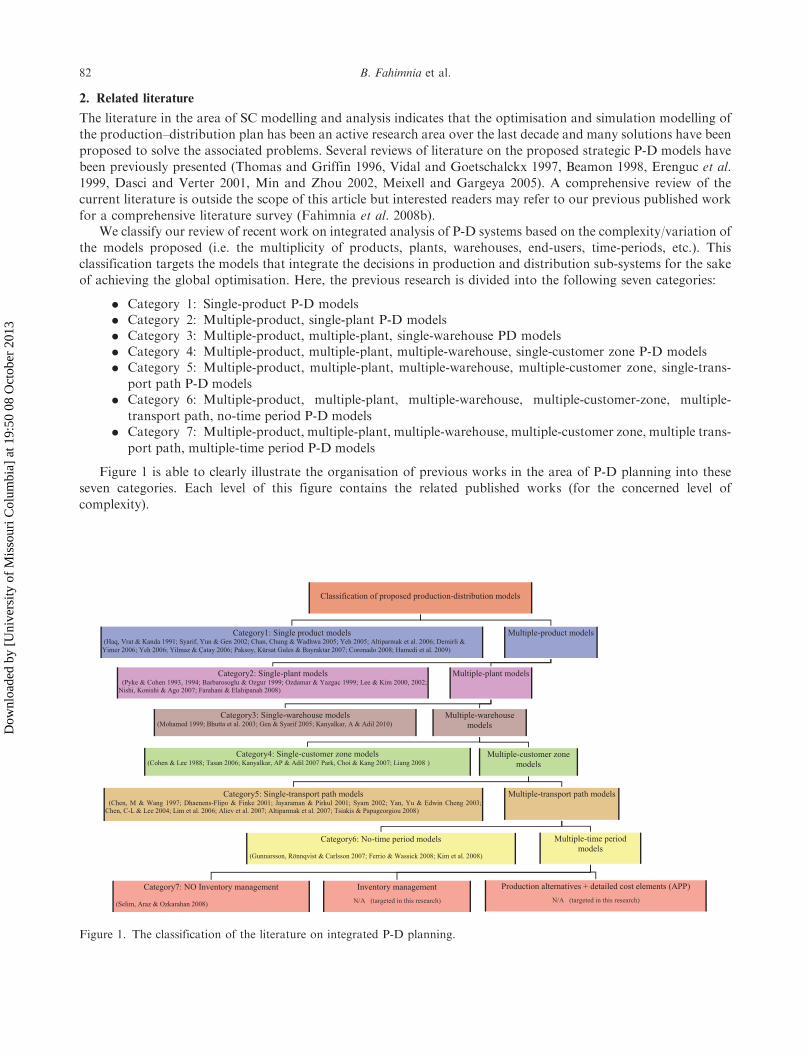
Figure 1 is able to clearly illustrate the organisation of previous works in the area of P-D planning into these
seven categories. Each level of this figure contains the related published works (for the concerned level of
complexity).
Classification of proposed production-distribution models
Category1: Single product models (Haq, Vrat & Kanda 1991; Syarif, Yun & Gen 2002; Chan, Chung & Wadhwa 2005; Yeh 2005; Altiparmak et al. 2006; Demirli & Yimer 2006; Yeh 2006; Yilmaz & Çatay 2006; Paksoy, Kürsat Gules & Bayraktar 2007; Coronado 2008; Hamedi et al. 2009)
Multiple-product models
Category2: Single-plant models (Pyke & Cohen 1993, 1994; Barbarosoglu & Ozgur 1999; Ozdamar & Yazgac 1999; Lee & Kim 2000, 2002; Nishi, Konishi & Ago 2007; Farahani & Elahipanah 2008)
Multiple-plant models
Category3: Single-warehouse models (Mohamed 1999; Bhutta et al. 2003; Gen & Syarif 2005; Kanyalkar, A & Adil 2010)
Multiple-warehouse models
Category4: Single-customer zone models (Cohen & Lee 1988; Tasan 2006; Kanyalkar, AP & Adil 2007 Park, Choi & Kang 2007; Liang 2008 )
Multiple-customer zone models
Category5: Single-transport path models (Chen, M & Wang 1997; Dhaenens-Flipo & Finke 2001; Jayaraman & Pirkul 2001; Syam 2002; Yan, Yu & Edwin Cheng 2003; Chen, C-L & Lee 2004; Lim et al. 2006; Aliev et al. 2007; Altiparmak et al. 2007; Tsiakis & Papageorgiou 2008)
Multiple-transport path models
Category6: No-time period models (Gunnarsson, Rönnqvist & Carlsson 2007; Ferrio & Wassick 2008; Kim et al. 2008)
Multiple-time period models
Production alternatives + detailed cost elements (APP) N/A (targeted in this research)
Inventory management N/A (targeted in this research)
Category7: NO Inventory management
(Selim, Araz & Ozkarahan 2008)
Figure 1. The classification of the literature on integrated P-D planning.
82 B. Fahimnia et al.
Dow
nloa
ded
by [
Uni
vers
ity o
f M
isso
uri C
olum
bia]
at 1
9:50
08
Oct
ober
201
3
This classification allows us to identify the important areas where further research is required. We classify thegaps in the current literature into the following two main categories:
(1) The first and probably the most crucial issue is oversimplification in the proposed models, mainly due to thecomplexities associated with the optimisation of real-life P-D plans.
(2) There is a large potential to further improve the quality and precision of the proposed solution approachesfor the optimisation of integrated P-D planning problems.
This article aims to address the two identified gaps. In tackling the oversimplifications in the past models, thisresearch proposes a new methodology for the optimisation of P-D plan integrating Aggregate Production Plan andDistribution Plan. The model incorporates the following characteristics:
. Multiple product types
. Multiple manufacturing plants
. Multiple machine centres at each manufacturing plant
. A stack buffer at each plant temporarily storing finished products
. All possible in-house/outsource alternatives
. Detailed production cost components (as in APP)
. Multiple warehouses (distribution centres)
. Multiple end-users
. Multiple transport routs (direct or indirect shipment from plants to end users)
. Effective inventory management (both Work-in-Progress inventory and inventory of finished products)
. The possibility of backlogging at end-users
. Multiple time periods
Different tools and techniques have been used in past studies for the optimisation of the P-D plan.Mathematical techniques which have been widely used in the past include Linear Programming models (Chen andWang 1997, Kanyalkar and Adil 2005, 2007, 2008, Liang 2008), Mixed Integer Programming models (Haq et al.1991, Mohamed 1999, Dhaenens-Flipo and Finke 2001, Bhutta et al. 2003, Yan et al. 2003, Chen and Lee 2004,Demirli and Yimer 2006, Gunnarsson et al. 2007, Paksoy et al. 2007, Ferrio and Wassick 2008, Kim et al. 2008,Selim et al. 2008, Tsiakis and Papageorgiou 2008, Hamedi et al. 2009), and Lagrangian Relaxation models(Barbarosoglu and Ozgur 1999, Jayaraman and Pirkul 2001, Syam 2002, Nishi et al. 2007). Some heuristictechniques have also been employed for this purpose (Cohen and Lee 1988, Pyke and Cohen 1993, 1994, Ozdamarand Yazgac 1999, Jayaraman and Ross 2003, Yeh 2005, Yilmaz and Catay 2006, Coronado 2008). Also, someprevious studies have analysed the capability of simulation modelling in SC planning (Ritchie-Dunham et al. 2000,Jain, et al. 2001, Persson and Olhager 2002, Williams and Gunal 2003, Moyaux et al. 2004, Lim et al. 2006).
However, using traditional methods based on linear and non-linear programming to find the optimal solutionfor such a complex P-D model is almost impossible or subject to heavy computing overheads (Fahimnia et al.2009b). Also, the heuristic and simulation techniques which are able to tackle more complex scenarios cannot provethe optimality of the solutions found and do not have the potential to find the optimal solution on their own(Noor 2008).
GAs have shown to be a highly effective and efficient tool in solving complex optimisation problems and some oftheir successful applications in the optimisation of supply chain models have been proposed in literature (Syarifet al. 2002, Altiparmak et al. 2005, 2006, 2007, Chan et al. 2005, Gen and Syarif 2005, Tasan 2006; Yeh 2006, Alievet al. 2007, Park et al. 2007, Farahani and Elahipanah 2008, Liang 2008). GA is chosen as the appropriate tool forthe optimisation of P-D plan in this article due to its following capabilities:
. it is capable of handling large search spaces easily;
. in terms of speed, GA conducts a search through the space of solutions by exploiting a population of pointsin parallel rather than a single point; therefore, is faster than other techniques in handling hugeoptimisation problems;
. it creates a number of optimal solutions allowing the user to make the final decision;
. GA has great flexibility in defining the constraints and the quality measures;
. GA is effectively applicable for continuous and discrete problems.
To address the second gap identified in the current literature of P-D planning, a novel GA procedure isdeveloped in this article for the optimisation of the proposed complex P-D plan. To demonstrate the applicability of
International Journal of Production Research 83
Dow
nloa
ded
by [
Uni
vers
ity o
f M
isso
uri C
olum
bia]
at 1
9:50
08
Oct
ober
201
3
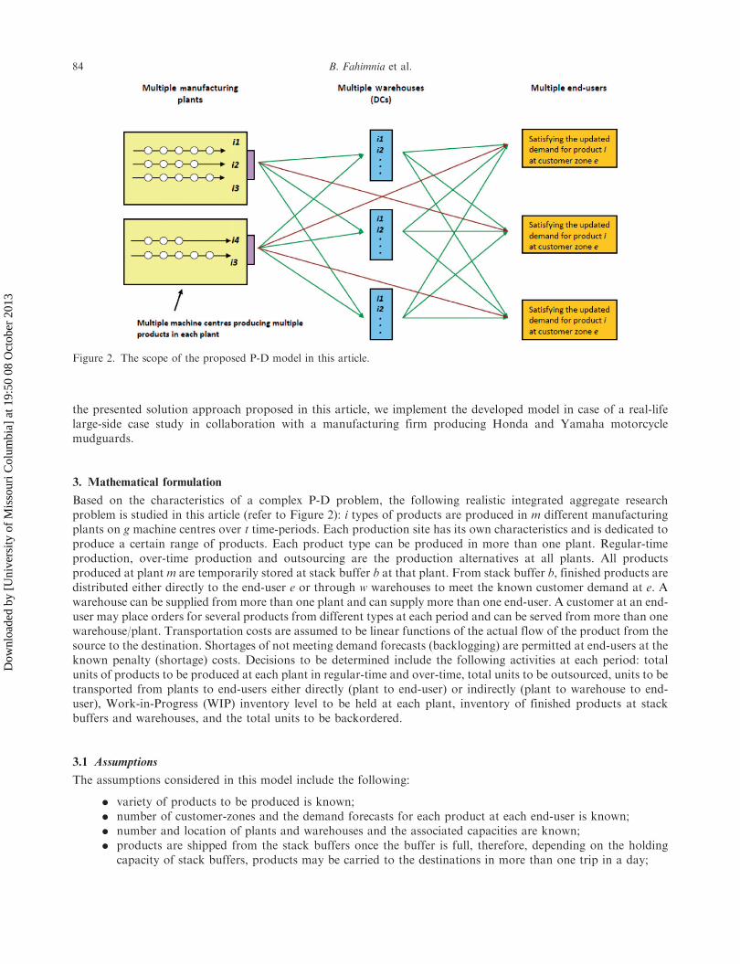
the presented solution approach proposed in this article, we implement the developed model in case of a real-lifelarge-side case study in collaboration with a manufacturing firm producing Honda and Yamaha motorcyclemudguards.
3. Mathematical formulation
Based on the characteristics of a complex P-D problem, the following realistic integrated aggregate researchproblem is studied in this article (refer to Figure 2): i types of products are produced in m different manufacturingplants on g machine centres over t time-periods. Each production site has its own characteristics and is dedicated toproduce a certain range of products. Each product type can be produced in more than one plant. Regular-timeproduction, over-time production and outsourcing are the production alternatives at all plants. All productsproduced at plant m are temporarily stored at stack buffer b at that plant. From stack buffer b, finished products aredistributed either directly to the end-user e or through w warehouses to meet the known customer demand at e. Awarehouse can be supplied from more than one plant and can supply more than one end-user. A customer at an end-user may place orders for several products from different types at each period and can be served from more than onewarehouse/plant. Transportation costs are assumed to be linear functions of the actual flow of the product from thesource to the destination. Shortages of not meeting demand forecasts (backlogging) are permitted at end-users at theknown penalty (shortage) costs. Decisions to be determined include the following activities at each period: totalunits of products to be produced at each plant in regular-time and over-time, total units to be outsourced, units to betransported from plants to end-users either directly (plant to end-user) or indirectly (plant to warehouse to end-user), Work-in-Progress (WIP) inventory level to be held at each plant, inventory of finished products at stackbuffers and warehouses, and the total units to be backordered.
3.1 Assumptions
The assumptions considered in this model include the following:
. variety of products to be produced is known;
. number of customer-zones and the demand forecasts for each product at each end-user is known;
. number and location of plants and warehouses and the associated capacities are known;
. products are shipped from the stack buffers once the buffer is full, therefore, depending on the holdingcapacity of stack buffers, products may be carried to the destinations in more than one trip in a day;
Figure 2. The scope of the proposed P-D model in this article.
84 B. Fahimnia et al.
Dow
nloa
ded
by [
Uni
vers
ity o
f M
isso
uri C
olum
bia]
at 1
9:50
08
Oct
ober
201
3
. capacity limitations for regular-time and over-time production (capacity of machine centres), restrictions on
capacity of raw material supply, limitations in storage capacity in stack buffers and warehouses and
distribution capacities are known;. WIP inventory levels and the inventory levels of finished products at stack buffers and warehouses at the
start and end of the planning horizon (t¼ 0 and t¼T ) are known;. orders for subcontracting items are made by each plant at the start of each period and the subcontractors
send the products directly to the stack buffer of the source plant (ordering plant) by the end of the ordering
period.
3.2 Parameters and decision variables
Indices for this model include: i for product type, m for plant, b for stack buffer, w for warehouse, e for end-user, t
for time period and g for machine centre. The parameters and decision variables for the proposed model are given in
Appendix A.
3.3 Objective function
The objective function (i.e. cost function) minimises the sum of the following costs:
(1) production costs in regular-time and over-time as well as outsourcing costs;(2) inventory holding costs;(3) transportation costs;(4) shortage costs.
Using the parameters and decision variables defined in the former section, the mixed-integer nonlinear formu-
lation in Equation (1) presents the objective function (cost function). This is followed by the detailed description of
the model constraints:
Min Z ¼Xt
Xm
OmtGmt þXi
Xm
Xt
IimtRPimtGmt þXi
Xm
Xt
I 0imtOPimtGmt þXi
Xm
Xt
I 00imtOSimtGmt
þXt
Xw
O 0wtG0wt þ
Xi
Xm
Xt
HimtXimtGmt þXi
Xb
Xm
Xt
H 0ibtYibt�bmGmt
þXi
Xw
Xt
H 00iwtZiwtG0wt þ
Xi
Xb
Xm
Xw
Xt
JibwtTibwt�bmGmtG0wtFibwt
þXi
Xw
Xe
Xt
J 0iwetT0iwetG
0wt F
0iwet þ
Xi
Xb
Xm
Xe
Xt
J 00ibetT00ibet�bmGmt F
00ibet
þXi
Xe
Xt
SietSCietdiet ð1Þ
In which :Xi
Xm
Xt
IimtRPimtGmt ¼Xi
Xm
Xt
IimtGmt
Xg
PigmtLigmt þ RMimt þ �imt
!" #ð2Þ
And :Xi
Xm
Xt
I 0imtOPimtGmt ¼Xi
Xm
Xt
I 0imtGmt
Xg
PigmtL0igmt þ RMimt þ �imt
!" #ð3Þ
Subject to the following constraints:
Iimt þ I 0imt � �imtGmt 8i,m, t ð4Þ
IfXi
Xg
Qigmt ¼
Pi
Pg Pigmt
28i,m, t
International Journal of Production Research 85
Dow
nloa
ded
by [
Uni
vers
ity o
f M
isso
uri C
olum
bia]
at 1
9:50
08
Oct
ober
201
3
Then:Xi
Xg
PigmtIimt þXi
Xg
PigmtI0imt þ
Xi
Xg
Qigmt Ximt � Ximðt�1Þ
� ��Xi
Xg
Gmt �igmt þ �0igmt
� �8i,m, t ð5Þ
Ximt � XMaximt 8i,m, t ð6Þ
Yibt � HCibt 8i, b,m, t ð7Þ
Ziwt � HC 0iwt 8i,w, t ð8Þ
Xw
Jibwt þXe
J 00ibet � Eibt�bmGmt 8i, b,m, t ð9Þ
Xe
J 0iwet � G 0wtE0iwt 8i,w, t ð10Þ
Xm
Xt
Iimt þ I 0imt þ I 00imt
� �¼Xe
Xt
Diet 8i ð11Þ
Siet � SMaxiet 8i, e, t ð12Þ
Yibt � Yibðt�1Þ ¼ Gmt ðIimt þ I 0imt þ I 00imtÞ � �bmXw
JibwtG0wt þ
Xe
J 00ibet
!" #8i, b,m, t ð13Þ
Ziwt � Ziwðt�1Þ ¼Xb
Jibwt�bmGmtG0wtFibwt �
Xe
J 0iwetG0wt F
0iwet 8i,w, t ð14Þ
Xw
J 0iwetG0wt þ
Xb
J 00ibet�bmGmt ¼ Diet � Siet � diet þ Sieðt�1Þ � dieðt�1Þ 8i, e, t ð15Þ
Xt¼0
Ximt ¼ �im andXt¼T
Ximt ¼ �0im 8i,m ð16Þ
Xt¼0
Yibt ¼ �ib andXt¼T
Yibt ¼ �0ib 8i, b ð17Þ
Xt¼0
Ziwt ¼ iw andXt¼T
Ziwt ¼ 0iw 8i,w ð18Þ
Iimt, I0imt, I
00imt,Ximt � 0 8i,m, t ð19Þ
Jibwt � 0 8i, b,w, t ð20Þ
J 0iwet � 0 8i,w, e, t ð21Þ
J 00ibet � 0 8i, b, e, t ð22Þ
Yibt � 0 8i, b, t ð23Þ
Ziwt � 0 8i,w, t ð24Þ
86 B. Fahimnia et al.
Dow
nloa
ded
by [
Uni
vers
ity o
f M
isso
uri C
olum
bia]
at 1
9:50
08
Oct
ober
201
3
Siet � 0 8i, e, t ð25Þ
The objective function in Equation (1) minimises the total production, inventory holding, transportation andshortage costs. To ease the reading and understanding of the objective function, Equations (2) and (3) give details ofthe production costs in regular-time and over-time respectively (i.e. referring to the second and third portions ofEquation (1) correspondingly). Equations (4)–(10) represent the capacity constraints. Equation (4) shows the rawmaterial supply capacity restrictions. Equation (5) is the production capacity constraint at manufacturing plants (i.e.limitation for regular-time and over-time production against machine centre capacity constraints). It should benoted that a WIP inventory is referred to as an incomplete item and the time it takes to produce a WIP inventory(Qigmt) is smaller than the time taken to produce a finished product (Pigmt). Equation (5) assumes that the averagetime to produce a WIP item is half of the time it takes to complete the item. The limitation in WIP inventory amountto be carried at each plant is represented in Equation (6). Stack buffer capacity restriction shown in Equation (7)implies the restriction on the stored products in the stack buffer at the end of a period. Equation (8) stands for thelimitations in warehouse holding capacity. The distribution capacity constraint from stack buffers and warehousesare represented in Equations (9) and (10), respectively. Equation (11) and (12) are demand and shortage constrain.Equation (11) implies that the total amount of production and outsourcing for every product at all plants must meetthe forecasted demand for that product at the end of the planning horizon (i.e. total satisfaction of all demands forevery product at the end of the planning phase). Equation (12) enforces the maximum allowed shortage at end-users.Balance constrains at stack buffers, warehouses and end-users are represented at Equations (13)–(18). Equation (13)represents the inventory balance constraint at stack buffers. Equations (14) and (15) are the balance equations atwarehouses and end-users. Constraint (15) ensures that the shipments of a product to an end-user either satisfy thedemand for that product at period t or some shortage would appear. Equations (16)–(18) determine the WIPinventory levels and the inventory levels of finished products at stack buffers and warehouses at the start and end ofthe planning horizon (t¼ 0 and t¼T ). Equations (19)–(25) demonstrate the ‘variables’ constrains enforcing non-negativity restriction for all the decision variables.
3.4 Constraint handling mechanism
A weighted technique is presented in this research as a mechanism ensuring the proper implementation of the majorconstraints in the proposed GA model. The proposed Constraints Handling Mechanism (CHM) aims to minimisethe violations of the constraint condition (the degree of infeasibility) by introducing a penalty cost indicating thefitness of solutions against the satisfaction of major constraints.
In the set of constraints for the developed P-D mode, Equations (5), (13)–(15) are the ‘major constraints’imposing the key restrictions on the production and inventory holding activities throughout the SC network. CHMscores each solution (each chromosome in the GA cycle) based on its fitness within the major constraints.
MinY ¼ AGmt
Xi
Xg
PigmtIimt þXi
Xg
PigmtI0imt þ
Xi
Xg
Qigmt Ximt � Ximðt�1Þ
� ��Xi
Xg
�igmt þ �0igmt
� �" #
þ BGmt �bm Yibt � Yibðt�1Þ þXw
JibwtG0mt þ
Xe
J 00ibet
!� Iimt þ I0imt þ I 00imt
� �" #
þ C G0wtðZiwt � Ziwðt�1ÞÞ �Xb
Jibwt�bmGmtG0wtFibwt þ
Xe
J0iwetG0wtF0iwet
" #
þDXw
J0iwetG0wt þ
Xb
J 00ibet�bmGmt
!�Diet þ Sietdiet � Sieðt�1Þdieðt�1Þ
" #ð26Þ
A, B, C and D in Equation (26) are the contribution coefficients for the major capacity constraints. Contributioncoefficients demonstrate the degree of contribution by each major constraint in scoring the solutions. Depending onthe organisation’s current policies and strategies (i.e. how flexible the company is in regards to each constraint), theoperation management team is able to determine the contribution coefficients in the way that: A þ B þ C þ D ¼ 1.Depending on the method chosen for the assignment of values to the contribution coefficients, CHM is able to makemedium to large influence on the optimisation results.
International Journal of Production Research 87
Dow
nloa
ded
by [
Uni
vers
ity o
f M
isso
uri C
olum
bia]
at 1
9:50
08
Oct
ober
201
3
4. Proposed GA
Figure 3 represents the GA procedure for the optimisation of the proposed P-D model. In this section, we discussthe stages/phases of this procedure in detail.
4.1 Chromosome representation
In the first stage (population), chromosomes are generated for an (experimentally) optimal population size. Figure 4shows the structure of a chromosome. The tree-based chromosome structure represents three levels: leaves (Level 3),trunk (Level 2) and the root (Level 1) of the tree.
From bottom up, level three (leaves/crown of the tree) contain the protean arrays standing for the 10 decisionvariables defined in Section 3.2. Level two in the middle (trunk of the tree) contains the objective functions forevaluating the fitness of a chromosome. Level one (root of the three) comprises the fitness function reflecting howgood a chromosome is based on its capability of achieving the minimum cost objective and satisfying the keyconstraints. Equation (27) uses a weight technique for defining the fitness function, in which " and � are the weight
Reproduction
New generation
Offsprings
Elitism
Manipulation
Evaluation (Fitness)• Objective function • Constraint handling mechanism
Figure 4. The proposed tree-based chromosome representation.
88 B. Fahimnia et al.
Dow
nloa
ded
by [
Uni
vers
ity o
f M
isso
uri C
olum
bia]
at 1
9:50
08
Oct
ober
201
3
factors (each between 0 and 1 and "þ �¼ 1) indicating the level of contribution for the objective function and CHM.The equal contribution of objective function and CHM is generally preferred for the first runs to avoid theconfusion in initial data analysis.
Fitness function ¼Min "ðObjective function valueÞ þ �ðThe value from the CHMÞ½ � ð27Þ
There are two main reasons why a tree-based configuration is considered as the chromosome structure. The firstreason is the high number of variables involved. Having a linear chromosome means having 10 groups of variableseach containing hundreds of genes. This obviously requires a lot of extra memory space and ultra high-speedprocessors for doing a certain process on a certain gene. The second reason is the encoding/decoding difficulties andthe complexity of applying constraints to every gene of variables. In the proposed tree-based structure, the length of‘Chromosome State’ is fixed at 10 arrays, while the actual length (i.e. the number of genes) is formed once theprogram is run (i.e. differs from run to run). Hence, this structure not only will ease the process of encoding/decoding, but it also allows a more adaptable design by offering the capability of easily changing the number ofvariables in various manufacturing/distribution scenarios.
4.2 Chromosome evaluation
In this step, chromosomes are filled in levels 1 and 2. The fitness of chromosomes in every generation (appeared atlevel 1) is calculated from Equation (27).
4.3 Selection process
A Tournament selection process is adopted for the proposed GA in which the two selected chromosomes from thepopulation (step 1) are compared based on their fitness value at level 1 and the fitter chromosome is copied into themating pool. The population of the mating pool is then checked and if it has not reached a certain amount the nextcouple of chromosomes will go through the tournament; otherwise, go to the next step.
4.4 Genetic operators
The new generation is produced through the application of genetic operators. However, when producing the newpopulation using genetic operators, there is a chance of losing the best found chromosomes. To prevent this fromhappening, elitism copies the fittest chromosome from the mating pool directly to the next generation. Elitism canbe more effective when the mutation rate is high and may cause the loss of good solutions in the next generation.
4.4.1 Multi-level multi-point crossover operator
Crossover is performed by exchanging the information of two parent chromosomes. We propose a multi-level multi-point crossover operator: (1) two chromosomes are randomly selected from the pool; (2) a random number (n)between 1 and 10 (i.e. number of variables’ sets at level 3) is generated. This implies the chromosome BreakingPoints (BP) where the crossover operator will occur along the length of each chromosome; (3) ‘n’ number ofvariables from the 10 available sets of variables are selected (at level 3); (4) for each selected chromosome a randomnumber (m) is created between 1 and the multiplication of all the indices of that variable (e.g. for variable I: n¼ 1and 14m4 i�m� t). This implies the Variable Breaking Point (VBP) where the crossover operator will operatealong BPs; (5) crossover operator occurs at VBPs; (6) the new generated chromosomes are then copied into thestep 1 (new generation). Crossover rate (the proportion of chromosomes in the mating pool on which the crossoveroperator will apply) is determined based on the trial-and-error practice.
4.4.2 Non-uniform mutation operator
We use mutation to modify one or more genes of an existing individual for increasing the variability of thepopulation. In the process of non-uniform mutation, a single chromosome is randomly selected from the pool.The mutation is then applied to a random number of genes on the selected chromosome. To do so,a (constrained) random number is added to or subtracted from the numeric amount of the selected genes.
International Journal of Production Research 89
Dow
nloa
ded
by [
Uni
vers
ity o
f M
isso
uri C
olum
bia]
at 1
9:50
08
Oct
ober
201
3
Once the mutation process is completed, the new generated chromosome is copied from the mating pool into thenew generation (step 1).
4.4.3 Modified swap operator
A simple swap mutation exchanges the values of two genes in one chromosome. As opposed to simple mutationoperator which applies on one single gene, the swap mutation interchanges the values between two genes. Therefore,instead of producing new values, the existing values are interchanged within one chromosome. In addition, unlikecrossover operator, a swap mutation operates within a single chromosome instead of swapping the gene valuesbetween the parents. In this way, new traits are produced in one chromosome to be evaluated in the next generation.The modified swap operator adapted in this study ensures that the randomly selected variables for swapping haveidentical min/max domains (ranges) and hence the swap operator does not assign out-of-range values by exchangingunmatchable values. For instance, swap operator can replace the value of I213 by its equivalent I341 (not by J1243).
First, we determine on which of the 10 sets of variables (at CS level) the swap operator will be implemented. Forthis reason, a random number, !, is generated, in the way that 15!5 10. In coding, this must be done in the wayto restrict ! for selecting only the interchangeable variable sets (e.g. I and I 0). For each !, a second random number() is generated which determines how many random swaps will occur along the selected variable strings. Swap rate(to be determined experimentally) will determine on what proportion of chromosomes in the mating pool the swapoperator will be applied.
4.5 Termination
Unfortunately, in all optimisation methods, it is always difficult to prove the convergence of the optimal solutionand therefore we set a termination point to stop the process. Depending on the level of precision required, therecan be two approaches for terminating the GA process: (1) by limiting the number of iterations/generations and(2) when minimal change in fitness value is observed in consecutive generations.
5. A real-world case study
5.1 Problem statement
To investigate the effectiveness of the proposed GA, a real-world case study was studied. PSP Co. is amanufacturing/distribution company producing Honda and Yamaha motorcycle mudguards. As in November2008, four types of products are produced in four manufacturing plants in different geographical locations. Honda125 front and rear mudguards as well as Yamaha 200 front and rear mudguards (i1 � i4, respectively). Plant 1 and 2(m1 and m2) are in major cities and have the facilities to produce all products. Plant 3 (m3 ) produces i1 and i2 andm4 is able to produce i1 and i3: All items are manufactured by passing through four machine centres (g1 � g4).Regular-time production, over-time production and outsourcing are available at all plants. Each plant has a stackbuffer temporarily storing the finished products (b1 � b4). Products can be distributed from manufacturing plantseither directly to five end-users (e1 � e5) or through six established warehouses (w1 � w6) in different locations.Planning horizon is two weeks (T¼ 12 days) and all the demand is to be satisfied at the end of the planning horizon(T¼ 12). Shortage of not meeting demand forecasts at the end of each period is allowed at known penalty costsdefined by each end-user.
The objective of this case study is to determine the PSP production allocation as well as the distributionstrategies during the planning horizon of 2 weeks in order to minimise the overall production and distribution costs.The proposed P-D plan for the next planning horizon needs to address how the demand for each product will besatisfied at each end-user. This will determine which item is produced at each manufacturing plant and how thefinished products are distributed to the end-users for satisfying the known market demands. Due to the high numberof variables and constraints involved in this case problem, finding the optimal solution has been an intricatechallenge for PSP. The proposed GA model in this article was implemented to search for the PSP optimal integratedP-D plan for the next planning horizon. It is demonstrated in the next section how the proposed optimisationmodel can yield significant cost reduction benefits for PSP (more than $510,000 per fortnight) through the globalintegration of production and distribution decisions within acceptable model runtime (about 12min).
90 B. Fahimnia et al.
Dow
nloa
ded
by [
Uni
vers
ity o
f M
isso
uri C
olum
bia]
at 1
9:50
08
Oct
ober
201
3
5.2 Computational results
The GA procedure was coded in Microsoft Visual Basic 6.0 using MS Excel as the program interface. The machine
used to run the program is a PC with an Intel Core2 Quad Processor Q9400, and with 4GB DDR RAM at
1066MHz. In order to track the evolution of fitness function and the rate of convergence, all the results were
recorded following every single generation for 1500 generations. The program was run several times for a
population size of 100 chromosomes, crossover rate of 0.6, mutation rate of 0.13 and swap rate of 0.1. Contribution
coefficients of fitness function (" and �) are set in the way to allocate equal contributions for CHM and objective
function.In all the test runs, the GA converges to optimality consistently with a typical reduction in overall costs of just
less than 10% (optimum overall cost of $4,826,643 comparing to the original P-D cost of $5,337,675). The best
known results are generally achieved between 1200 and 1300 generations in the sense that the difference between the
overall SC costs in 10 consecutive generations becomes less than $1. The results are shown numerically in Table 1
and graphically in Figure 5. The dashed blue line in Figure 5 shows the actual data obtained and the continuous
black line indicates the trends in cost reduction (chromosome evolution). Also, for a population size of 100
chromosomes, Table 2 below shows the detailed cost components for the four best chromosomes selected in four
constant intervals at generations 1, 501, 1001 and 1501.The trend in the achieved numerical results implies the reasonable convergence speed (i.e. about 12min in
average for 1500 iterations) and consistent evolution of fitness function. The promising outcomes of this case study
(about 10% cost-saving benefit for the case of PSP in about 12min of model runtime) make this model and its
implementation easily transferable and customisable for solving other complex problems in the context of SC
planning and optimisation. Overall, the algorithm can be used as an effective and efficient tool for the optimisation
of complex supply networks.
Table 1. Numerical results for the population size of 100.
Chromosome Overall P-D cost ($) Production cost ($) Distribution cost ($)
Aliev, R.A., et al., 2007. Fuzzy-genetic approach to aggregate production-distribution planning in supply chain management.
Information Sciences, 177 (20), 4241–4255.Altiparmak, F., Gen, M., and Lin, L. 2005. A genetic algorithm for supply chain network design. In: 35th international conference
on computers and industrial engineering, Istanbul Technical University, Istanbul, Turkey, 111–116.Altiparmak, F., et al., 2006. A genetic algorithm approach for multi-objective optimization of supply chain networks. Computers
and Industrial Engineering, 51 (1), 196–215.Altiparmak, F., et al., 2007. A steady-state genetic algorithm for multi-product supply chain network design. Computers and
Industrial Engineering, 56 (2), 521–537.Barbarosoglu, G. and Ozgur, D., 1999. Hierarchical design of an integrated production and 2-echelon distribution system.
European Journal of Operational Research, 118 (3), 464–484.Beamon, B.M., 1998. Supply chain design and analysis: models and methods. International Journal of Production Economics,
55 (3), 281–294.Bhutta, K.S., et al., 2003. An integrated location, production, distribution and investment model for a multinational corporation.
International Journal of Production Economics, 86 (3), 201–216.Chan, F.T.S., Chung, S.H., and Wadhwa, S., 2005. A hybrid genetic algorithm for production and distribution. Omega, 33 (4),
345–355.Chen, C.-.L. and Lee, W.-C., 2004. Multi-objective optimization of multi-echelon supply chain networks with uncertain product
demands and prices. Computers and Chemical Engineering, 28 (6–7), 1131–1144.Chen, M. and Wang, W., 1997. A linear programming model for integrated steel production and distribution planning.
International Journal of Operations and Production Management, 17 (6), 592–610.Cohen, M.A. and Lee, H.L., 1988. Strategic analysis of integrated production-distribution systems: models and methods.
Operations Research Society of America, 36 (2), 216–228.Coronado, J.L., 2008. An optimization model for strategic supply chain design under stochastic capacity disruptions. Texas: College
of Engineering, Texas A&M University.Dasci, A. and Verter, V., 2001. A continuous model for production-distribution system design. European Journal of Operational
Research, 129 (2), 287–298.Demirli, K. and Yimer, A.D., 2006. Production–distribution planning with fuzzy costs. Paper presented at the fuzzy information
processing society. NAFIPS 2006. Annual meeting of the North American, Concordia University, Montreal, Canada.Dhaenens-Flipo, C. and Finke, G., 2001. An integrated model for an industrial production-distribution problem. IIE
Transactions – Operations Engineering, 33 (9), 705–715.Erenguc, S.S., Simpson, N.C., and Vakharia, A.J., 1999. Integrated production/distribution planning in supply chains: an invited
review. European Journal of Operational Research, 115 (2), 219–236.
Fahimnia, B., Luong, L.H.S., and Marian, R. 2008a. An integrated model for the optimisation of a two-echelon supply network.
Journal of Achievements in Materials and Manufacturing Engineering, 31 (2), 477–484.
Fahimnia, B., Luong, L.H.S., and Marian, R., 2008b. Optimization/simulation modelling of the integrated production-
distribution plan: an innovative survey. WSEAS Transactions on Business and Economics, 5 (3), 44–57.
Fahimnia, B., Luong, L.H.S., and Marian, R. 2009a. Genetic algorithm optimization of a two-echelon supply chain
network. In: International Conference on Industrial Engineering and Systems Management (IESM’ 2009), Montreal,
Canada.Fahimnia, B., Luong, L.H.S., and Marian, R. 2009b. Optimization and performance evaluation of an integrated production–
distribution plan in supply chains. ASME International Mechanical Engineering Congress and Exposition (IMECE2009).
Florida, USA: American Society of Mechanical Engineering.Farahani, R.Z. and Elahipanah, M., 2008. A genetic algorithm to optimize the total cost and service level for just-in-time
distribution in a supply chain. International Journal of Production Economics, 111 (2), 229–243.Ferrio, J. and Wassick, J., 2008. Chemical supply chain network optimization. Computers and Chemical Engineering, 32 (11),
2481–2504.Gen, M. and Syarif, A., 2005. Hybrid genetic algorithm for multi-time period production/distribution planning. Computers and
Industrial Engineering, 48 (4), 799–809.Gunnarsson, H., Ronnqvist, M., and Carlsson, D., 2007. Integrated production and distribution planning for Sodra cell AB.
Journal of Mathematical Modelling and Algorithms, 6 (1), 25–45.Hamedi, M., et al., 2009. A distribution planning model for natural gas supply chain: a case study. Energy Policy, 37 (3),
799–812.Haq, A.N., Vrat, P., and Kanda, A., 1991. An integrated production-inventory-distribution model for manufacture of urea: a
case. International Journal of Production Economics, 25 (1–3), 39–49.Jain, S., et al., 2001. Development of a high-level supply chain simulation model. In: Proceedings of the winter simulation
conference, Artington, VA, USA.
International Journal of Production Research 93
Dow
nloa
ded
by [
Uni
vers
ity o
f M
isso
uri C
olum
bia]
at 1
9:50
08
Oct
ober
201
3
Jayaraman, V. and Pirkul, H., 2001. Planning and coordination of production and distribution facilities for multiple
commodities. European Journal of Operational Research, 133 (2), 394–408.Jayaraman, V. and Ross, A., 2003. A simulated annealing methodology to distribution network design and management.
European Journal of Operational Research, 144 (3), 629–645.Kanyalkar, A. and Adil, G., 2005. An integrated aggregate and detailed planning in a multi-site production environment using
linear programming. International Journal of Production Research, 43 (20), 4431–4454.Kanyalkar, A. and Adil, G., 2007. Aggregate and detailed production planning integrating procurement and distribution plans in
a multi-site environment. International Journal of Production Research, 45 (22), 5329–5353.Kanyalkar, A. and Adil, G. 2010. A robust optimisation model for aggregate and detailed planning of a multi-site procurement-
production-distribution system. International Journal of Production Research, 48 (3), 635–656.Kim, Y., et al., 2008. An integrated model of supply network and production planning for multiple fuel products of multi-site
refineries. Computers and Chemical Engineering, 32 (11), 2529–2535.Lee, Y.H. and Kim, S.H. 2000. Optimal production-distribution planning in supply chain management using a hybrid
simulation-analytic approach. In: Proceedings of the winter simulation conference, San Diego, CA, USA.Lee, Y.H. and Kim, S.H., 2002. Production-distribution planning in supply chain considering capacity constraints. Computers
and Industrial Engineering, 43 (1–2), 169–190.Liang, T.-F., 2008. Fuzzy multi-objective production/distribution planning decisions with multi-product and multi-time period in
a supply chain. Computers and Industrial Engineering, 55 (3), 676–694.Lim, S.J., et al., 2006. A simulation approach for production-distribution planning with consideration given to replenishment
policies. The International Journal of Advanced Manufacturing Technology, 27 (5), 593–603.Meixell, M.J. and Gargeya, V.B., 2005. Global supply chain design: a literature review and critique. Transportation Research Part
E: Logistics and Transportation Review, 41 (6), 531–550.Min, H. and Zhou, G., 2002. Supply chain modeling: past, present and future. Computers and Industrial Engineering, 43 (1–2),
231–249.Mohamed, Z.M., 1999. An integrated production-distribution model for a multi-national company operating under varying
exchange rates. International Journal of Production Economics, 58 (1), 81–92.Moyaux, T., Chaib-draa, B., and D’Amours, S. 2004. Multi-agent simulation of collaborative strategies in a supply chain.
In: Proceedings of the third international joint conference on autonomous agents and multiagent systems, Washington DC,
USA.
Nishi, T., Konishi, M., and Ago, M., 2007. A distributed decision making system for integrated optimization of
production scheduling and distribution for aluminum production line. Computers and Chemical Engineering, 31 (10),
1205–1221.Noor, A.M.L. 2008. An integrated model for optimising manufacturing and distribution network scheduling. PhD thesis. School of
Advanced manufacturing and Mechanical Engineering, University of South Australia.Ozdamar, L. and Yazgac, T., 1999. A hierarchical planning approach for a production-distribution system. International Journal
of Production Research, 37 (16), 3759.Paksoy, T., Kursat Gules, H., and Bayraktar, D., 2007. Design and optimization of a strategic production–distribution model for
supply chain management: case study of a plastic profile manufacturer in Turkey. Selcuk Journal of Applied Mathematics,
8 (2), 83–99.Park, B., Choi, H., and Kang, M. 2007. Integration of production and distribution planning using a genetic algorithm in supply
chain management. In: P. Melin, O. Castillo, E.G. Ramırez, J. Kacprzyk and W. Pedrycz, eds. Analysis and design of
intelligent systems using soft computing techniques. Berlin: Springer, 416–426.Persson, F. and Olhager, J., 2002. Performance simulation of supply chain designs. International Journal of Production
Economics, 77 (3), 231–245.Pyke, D.F. and Cohen, M.A., 1993. Performance characteristics of stochastic integrated production-distribution systems.
European Journal of Operational Research, 68 (1), 23–48.Pyke, D.F. and Cohen, M.A., 1994. Multiproduct integrated production-distribution systems. European Journal of Operational
Research, 74 (1), 18–49.Ritchie-Dunham, J., et al., 2000. A strategic supply chain simulation model. In:Proceedings of the winter simulation conference,
Orlando, FL, USA.Selim, H., Araz, C., and Ozkarahan, I., 2008. Collaborative production-distribution planning in supply chain: a fuzzy
goal programming approach. Transportation Research Part E: Logistics and Transportation Review, 44 (3), 396–419.Syam, S.S., 2002. A model and methodologies for the location problem with logistical components. Computers and Operations
Research, 29 (9), 1173–1193.Syarif, A., Yun, Y., and Gen, M., 2002. Study on multi-stage logistic chain network: a spanning tree-based genetic algorithm
approach. Computers and Industrial Engineering, 43 (1–2), 299–314.Tasan, A. 2006. A two step approach for the integrated production and distribution planning of a supply chain. In: D.-S. Huang,
K. Li and G.W. Irwin, eds. Intelligent computing. Berlin: Springer, 883–888.
94 B. Fahimnia et al.
Dow
nloa
ded
by [
Uni
vers
ity o
f M
isso
uri C
olum
bia]
at 1
9:50
08
Oct
ober
201
3
Thomas, D.J. and Griffin, P.M., 1996. Coordinated supply chain management. European Journal of Operational Research, 94 (1),
1–15.
Tsiakis, P. and Papageorgiou, L.G., 2008. Optimal production allocation and distribution supply chain networks. International
Journal of Production Economics, 111 (2), 468–483.Vidal, C.J. and Goetschalckx, M., 1997. Strategic production-distribution models: a critical review with emphasis on global
supply chain models. European Journal of Operational Research, 98 (1), 1–18.Williams, E.J. and Gunal, A., 2003. Supply chain simulation and analysis with SIMFLEX. In: Proceedings of the winter
simulation conference, Dearborn, MI, USA.
Yan, H., Yu, Z., and Edwin Cheng, T.C., 2003. A strategic model for supply chain design with logical constraints: formulation
and solution. Computers and Operations Research, 30 (14), 2135–2155.Yeh, W.-C., 2005. A hybrid heuristic algorithm for the multistage supply chain network problem. The International Journal of
Advanced Manufacturing Technology, 26 (5–6), 675–685.Yeh, W.-C., 2006. An efficient memetic algorithm for the multi-stage supply chain network problem. The International Journal of
Advanced Manufacturing Technology, 29 (7), 803–813.Yilmaz, P. and Catay, B., 2006. Strategic level three-stage production distribution planning with capacity expansion. Computers
and Industrial Engineering, 51 (4), 609–620.
Appendix A
A.1 Model parameters
Diet Forecasted demand for product i at end-user e in period tOmt Fixed costs of opening and operating plant m in period tO 0wt Fixed costs of opening and operating warehouse w in period tHimt Unit WIP inventory holding cost for product i at plant m in period tH 0ibt Unit holding cost for finished product i at stack buffer b in period t
H 00iwt Unit holding cost for finished product i at warehouse w in period t
HCibt Holding capacity (maximum units) at stack buffer b for product i in period tHC 0iwt Holding capacity (units) at warehouse w for product i in period t
XMaximt Maximum allowed WIP inventory for the finished product i carried in plant m at the end of period t
Tibwt Unit transportation cost for product i from stack buffer b to warehouse w in period tT 0iwet Unit transportation cost for product i from warehouse w to end-user e in period tT 00ibet Unit transportation cost for product i directly from stack buffer b to end-user e in period t
RPimt Unit regular-time production cost of product i at plant m in period tOPimt Unit over-time production cost of product i at plant m in period tOSimt Unit outsourcing cost of product i ordered by plant m in period tPigmt Processing time to produce a unit of product i on g at plant m in period tQigmt Average time spent to produce a WIP unit of product i on g at plant m in period tLigmt Labour/hour cost for regular-time production of product i on g at plant m in period tL 0igmt Labour/hour cost for over-time production of product i on g at plant m in period t
RMimt Cost of raw material for producing a unit of product i at plant m in period t
�imt Variable overhead costs of regular-time production of product i at plant m in period t�imt Variable overhead costs of over-time production of product i at plant m in period t
SCiet Unit shortage cost (backordering - not meeting demand forecast) for product i at end-user e in period tSMaxiet Maximum amount of shortage permitted (maximum backorder) for product i at end-user e in period t�igmt Capacity hours for regular-time production of product i on g at plant m in period t� 0igmt Capacity hours for over-time production of product i on g at plant m in period t�imt Capacity units of raw material supply for product i at plant m in period tEibt The distribution capacity at stack buffer b for product i in period tE 0iwt The distribution capacity at warehouse w for product i in period t�im WIP inventory level of product i in plant m at the start of planning horizon (t¼ 0)� 0im WIP inventory level of product i in plant m at the end of planning horizon (t¼T )�ib Inventory level of product i in stack buffer b at the start of planning horizon (t¼ 0)� 0ib Inventory level of product i in stack buffer b at the end of planning horizon (t¼T )iw Inventory level of product i in warehouse w at the start of planning horizon (t¼ 0) 0iw Inventory level of product i in warehouse w at the end of planning horizon (t¼T )
�bm ¼1 If stack buffer b is located in plant m
0 Otherwise
�
International Journal of Production Research 95
Dow
nloa
ded
by [
Uni
vers
ity o
f M
isso
uri C
olum
bia]
at 1
9:50
08
Oct
ober
201
3
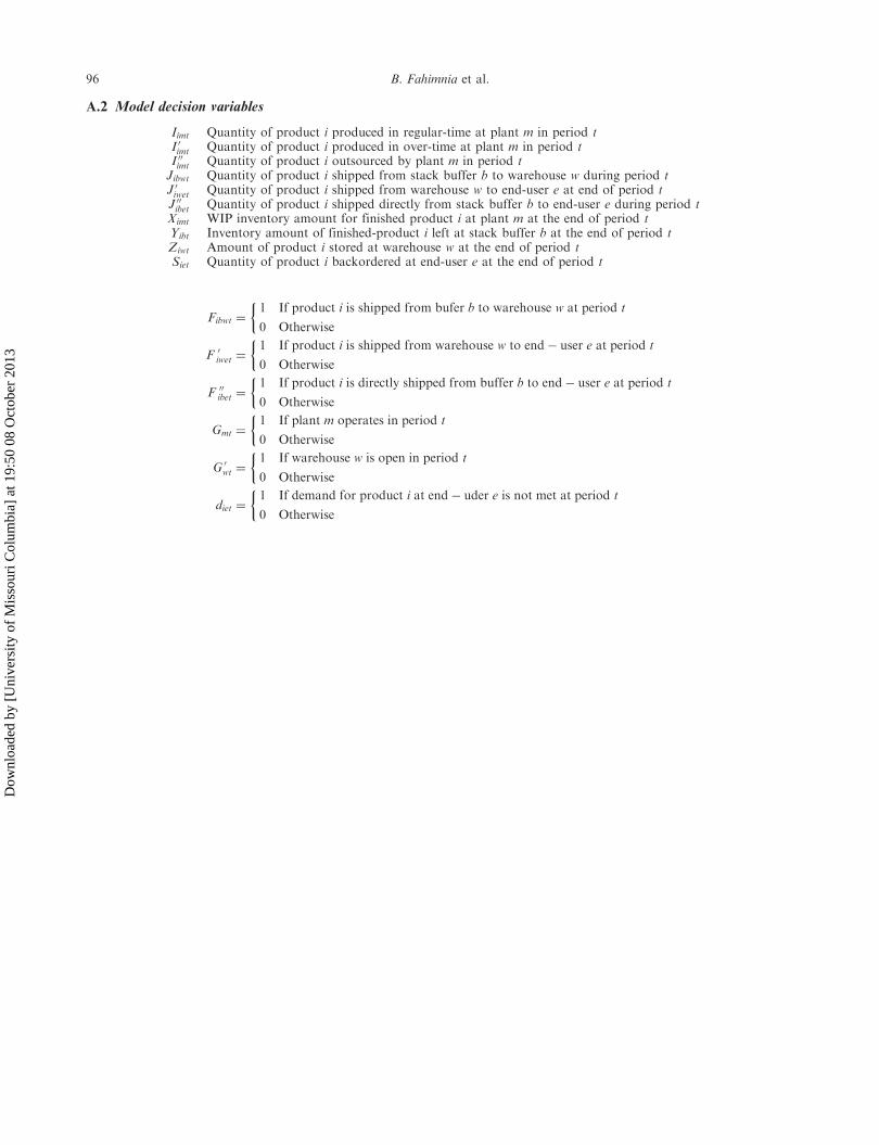
A.2 Model decision variables
Iimt Quantity of product i produced in regular-time at plant m in period tI 0imt Quantity of product i produced in over-time at plant m in period tI 00imt Quantity of product i outsourced by plant m in period tJibwt Quantity of product i shipped from stack buffer b to warehouse w during period tJ 0iwet Quantity of product i shipped from warehouse w to end-user e at end of period tJ 00ibet Quantity of product i shipped directly from stack buffer b to end-user e during period tXimt WIP inventory amount for finished product i at plant m at the end of period tYibt Inventory amount of finished-product i left at stack buffer b at the end of period tZiwt Amount of product i stored at warehouse w at the end of period tSiet Quantity of product i backordered at end-user e at the end of period t
Fibwt ¼1 If product i is shipped from bufer b to warehouse w at period t
0 Otherwise
�
F 0iwet ¼1 If product i is shipped from warehouse w to end� user e at period t
0 Otherwise
�
F 00ibet ¼1 If product i is directly shipped from buffer b to end� user e at period t
0 Otherwise
�
Gmt ¼1 If plant m operates in period t
0 Otherwise
�
G 0wt ¼1 If warehouse w is open in period t
0 Otherwise
�
diet ¼1 If demand for product i at end� uder e is not met at period t