1 Genetic Algorithm Synthesis of Four-bar Mechanisms Gerald P. Roston [email protected]Cybernet Systems Corporation Ann Arbor, MI 48105 Robert H. Sturges [email protected]Department of Mechanical Engineering Carnegie Mellon University Pittsburgh, PA 15217 Abstract The synthesis of four-bar mechanisms is well understood, classical design problem. The original systematic work in this field began in the late 1800’s and continues to be an active area of research. Limitations to the classical theory of four-bar synthe- sis potentially limit its application to certain real-world problems by virtue of the small number of precision points and unspecified order. This paper presents a numerical technique for four-bar mechanism synthesis based on genetic algorithms that removes this limitation by relaxing the accuracy of the precision points. 1 Introduction The analysis and synthesis of planar mechanisms has been actively studied since the last century. The pioneering work in this field was explored by Reuleaux in the 1870’s, and continues to be a field of active research. One of the great successes of this work was the development of the Burm- ester theory. This theory can be used to predict the number of different possible mechanisms that can be constructed to pass through a set of specified points (referred to in the kinematic literature as precision points). In brief, what this theory shows is that a four-bar mechanism can be built that will pass through five specified precision points, or through fewer specified precision points, but in a specified order. This solution, while graphical in its origin, is closed form and can be imple- mented on a computer, Sandor and Erdman (1984) and Shigley and Uicker (1980). The mechanisms produced using Burmester theory are “perfect” in the sense that they pass thought the precision points exactly, thus the justification for the term “precision point”. However, what if a four-bar mechanism is required to pass through more than five points? Burmester theory tells us that — except in some limited, special cases, such as symmetry. See the discussion on point position reduction in Hain (1967) — such a mechanism can not be built. What if the designer is able to relax the inherent exactness of the Burmester theory results and accept a mechanism that comes “close” to the specified points? This paper presents a method for synthesizing planar mech- anisms in answer to these questions. This paper is motivated by the desire to develop genetic design methods for complex sys- tems, of which mechanisms are expected to play a part. For further discussions of more general methods, and application of these methods to other problems, the reader is referred to Roston (1994) and Roston and Sturges (1995).
Transcript
1
Genetic Algorithm Synthesis of Four-bar MechanismsGerald P. Roston
Department of Mechanical EngineeringCarnegie Mellon University
Pittsburgh, PA 15217
Abstract
The synthesis of four-bar mechanisms is well understood, classical design problem.The original systematic work in this field began in the late 1800’s and continues tobe an active area of research. Limitations to the classical theory of four-bar synthe-sis potentially limit its application to certain real-world problems by virtue of thesmall number of precision points and unspecified order. This paper presents anumerical technique for four-bar mechanism synthesis based on genetic algorithmsthat removes this limitation by relaxing the accuracy of the precision points.
1 IntroductionThe analysis and synthesis of planar mechanisms has been actively studied since the last century.The pioneering work in this field was explored by Reuleaux in the 1870’s, and continues to be afield of active research. One of the great successes of this work was the development of the Burm-ester theory. This theory can be used to predict the number of different possible mechanisms thatcan be constructed to pass through a set of specified points (referred to in the kinematic literatureas precision points). In brief, what this theory shows is that a four-bar mechanism can be built thatwill pass through five specified precision points, or through fewer specified precision points, butin a specified order. This solution, while graphical in its origin, is closed form and can be imple-mented on a computer, Sandor and Erdman (1984) and Shigley and Uicker (1980).
The mechanisms produced using Burmester theory are “perfect” in the sense that they passthought the precision points exactly, thus the justification for the term “precision point”. However,what if a four-bar mechanism is required to pass through more than five points? Burmester theorytells us that — except in some limited, special cases, such as symmetry. See the discussion on pointposition reduction in Hain (1967) — such a mechanism can not be built. What if the designer isable to relax the inherent exactness of the Burmester theory results and accept a mechanism thatcomes “close” to the specified points? This paper presents a method for synthesizing planar mech-anisms in answer to these questions.
This paper is motivated by the desire to develop genetic design methods for complex sys-tems, of which mechanisms are expected to play a part. For further discussions of more generalmethods, and application of these methods to other problems, the reader is referred to Roston(1994) and Roston and Sturges (1995).
2
This paper is divided into five sections. First, a brief description of genetic algorithms is pro-vided in Section 2. Section 3 then describes the genetic representation for four-bar mechanismsused in this work. Section 4 describes the method used to solve for the positions of the mechanism.The key component of this work is the evaluation function, which is described in Section 5.Section 6 describes test results for a number of illustrative problems using this method.
2 Introduction to genetic algorithmsGenetic algorithms (GA) are search algorithms that use the notions of natural selection and genet-ics. The basic process used is survival of the fittest, with information exchange among the survi-vors. Like biological systems, there is some randomness to this process, but instead of causingdetrimental affects, this randomness gives GA robustness and the ability to generate better solu-tions.
One important fact to note is that although GA use random numbers, (unlike other techniquesthat use random numbers, such as simulated annealing) this search technique is not directionless.This technique makes use of past events to guide future events and yields continually improvingperformance of the functions being sought. This section is not intended to present the theory of GA,but rather to give the reader a familiarity with these techniques. Numerous references detail thecompleteness and correctness of GA and the interested reader is referred to Goldberg (1989), forexample.
Genetic algorithms differ from traditional optimization techniques in four fundamental ways :•GA work with a coding of the parameters, not the parameters themselves•GA use a population of samples, not a single sample•GA use payoff information, not auxiliary information or derivatives•GA use probabilistic, not deterministic, transition rules
The key to the successful implementation of a GA is the parameter coding. (The underlyingmathematical theory that explains GA is called schemata theory, see Holland (1976) for details.The primary selection operation, fitness proportionate reproduction (see page 4), has been shownmathematically to be near optimal in some senses.)
Once the parameter coding is completed, the solution of an optimization problem using GAproceeds according to the algorithm in Figure 1:Parameter coding is now described, followed by a discussion of each of the steps of the algorithm.
The most common type of GA used to date are bit-string genetic algorithms. These GA rep-resent the parameters by a binary string. Non-binary representations are possible but tend to bemore complex without yielding significant benefit. Binary numbers can be used to represent arbi-trarily large integral values. Non integral values can be represented by operating on an integralvalues. For example, real numbers, r, from 0.0 to 10.0 can be represented with a 10 bit binary stringand
(1)
where string is the decimal equivalent of the 10 bit binary string. It is important to note that thismethod of representation is noncontinuous, and it is possible that the optimal answer cannot beexactly expressed. For example, irrational numbers cannot be represented using this scheme. How-
r string 1024⁄=
3
ever, in practice, the required precision of the answer is known and a properly conceived parameterrepresentation will yield answers of sufficient accuracy.
Bit strings can be used to encode more than one number. They can incorporate any numberof parameters that are necessary for the problem. In this sense, bit strings are analogous to chromo-somes. A group of bits that defines a feature is called a gene and the values taken on by the bits arealleles.
The first step in the genetic algorithm is to determine an appropriate population size and thento create an initial population. Population size can be determined by applying an estimate based ontheoretical results or empirically. The composition of the initial population is determined ran-domly. The next step of the procedure is to evaluate the members of the population.
The value returned by the evaluation function for an individual is referred to as the individ-ual’s fitness. The evaluation function must meet three general rules:
1. Fitness values should be non-negative.2. Better individuals should have larger fitness scores.3. Evaluation functions should execute quickly, if possible.
Rule 1 is needed because of the selection process. Fitness values can be scaled to make negativevalues nonnegative or all negative values can simply be set to zero. Rule 2 is needed to promoteselection of fitter individuals for reproduction. The selection process will be shown to be a functionof the individuals’ fitnesses. The larger the fitness, i.e., the better the individual, the greater is itsprobability of reproducing. Finally, Rule 3 is needed for pragmatic reasons, since the solution timeis a linear function of the execution time of the evaluation function.
To mitigate the probability of premature convergence, fitness scaling is frequently used. Fit-ness scaling expands or contracts the range of fitness values to fit some predetermined range. Thereare numerous schemes for fitness scaling, one of the most common is linear scaling. Using thistechnique, the maximum fitness is defined to be n times the average fitness, and all other fitnessesare scaled accordingly. A typical value for n is 2.0. Fitness scaling has the dual advantages of pre-serving genetic diversity in an early population by preventing a small number of chromosomesfrom dominating the pool of surviving individuals preferentially selecting marginally better indi-viduals in well established populations.
The requirements for the evaluation function are similar to the requirements for evaluationfunctions for other types of optimization algorithms. Where GA radically depart from other algo-rithms is how they generate the next points to be evaluated. For example, calculus basedoptimization techniques use knowledge of the functions’ derivatives to “hill climb” towards anoptimal result. GA, however, use the “random” contributions of successful individuals in one gen-eration to produce individuals for the next generation. This method is neither continuous orcombinatorial. The first step of this process is selecting those members to be used to produce thenext generation.
There are a number of selection algorithms commonly used. The most basic selection algo-rithm is stochastic sampling with replacement. To visualize this scheme, imagine a weightedroulette wheel that is partitioned according to fitness of the individuals, Figure 2.“Spinning” this wheel many times will yield a higher percentage of those individuals with higherfitnesses and a lower percentage of those with lower fitnesses. The problem with this method isthat it is too random, and nonrepresentative populations are frequently observed. An scheme that
4
yields a more representative distribution is called remainder stochastic sampling without replace-ment . Using this method, the individuals comprising the next generation are found using a threestep procedure: First, the expected number of copies that the individuals in the current generationare expected to contribute to the next generation is calculated. Second, all members with anexpected number of copies greater than one contribute a number of copies of themselves equal tothe integral part of the expected number of copies. Finally, the remainder of the succeeding gener-ation is found probabilistically using the fractional part of the expected number of copies andremoving from consideration a member once it has been selected.
Once the members of the next generation have been selected, a three step process is used tomodify those individuals. The first step determines if a pair of individuals selected for reproductionwill be crossed or not based on a fixed probability. Experiments indicate that a crossover probabil-ity of 60% yields good results. The second step, for those members that are to be crossed, is toselect a crossover point and to perform the crossover operation, see Figure 5. There are three typesof crossover operations typically used, one-point, two-point and uniform . (Throughout this work,only single point crossover is used. For further discussions of the applicability of different cross-over algorithms, see De Jong and Spears (1992).) For all three crossover algorithms, the crossoverpoint(s) are chosen randomly. For the third step, the user defines a mutation probability, usually onthe order of one mutation per one thousand bits. Mutation is not the dominant force in a GA, but itis useful in restoring bits that may have been removed from a population at an earlier time.
3 GA representation of a four-bar mechanismFigure 3 shows a sketch of a four-bar mechanism. This mechanism can be described by nine inde-pendent variables which are illustrated in the sketch. The small triangles represent revolute jointsaffixed to the ground, the open circles represent revolute joints that join two links, and the filledcircle is the coupler point. Link 1 is the input link, the crank; the large shaded triangle is link 2, thecoupler; link 3 is the output link, the follower and link 4 is the ground. Also shown are the offsetsfrom the world origin and an angle that represents the angular offset of the coupler point.
When representing an object as a bit string, the easiest representation (for implementationpurposes) is one that uses the same number of bits as predefined computer types. In the C program-ming language, the basic types are char, short int, int and double, which are represented by 8,16, 32 and 64 bits respectively. For this problem, representing the variables with eight bits does notoffer sufficient precision to assure good results. For example, if the largest length representable is10, the granularity is approximately 0.04. By representing these lengths with 16 bits, the granular-ity is reduced to approximately 0.0002. For the work performed here, a mechanism’s chromosomeis represented by a 144 bit string as shown in Figure 4. Lengths are scaled from 0.0 to 10.0 andangles are scaled from 0.0 to 2π radians.
When representing a real quantity, such as length, as a bit string there are two important lim-itations: the range of values that the variable can assume and its granularity. If a solution requiresvalues larger than the largest representable value, the solution can not be found. If the solution issensitive to small variations in parameter values, it is possible that good solutions may only befound if the number of bits is increased. For this problem, using 16 bits instead of 8 increases thenumber of possible mechanisms from 4.7x10²¹ to 2.2x1043. In either case, the number of possiblemechanisms is so large that an exhaustive enumeration of the space is impractical.
5
A simple example of mechanism representation and crossover is shown in Figure 5. The leftside of this figure shows two mechanisms and their binary representations (the representations areactually shown in hexadecimal format for convenience). The right side of the figure shows theresult of crossing these two representations at the approximate location of the vertical line. Alsoshown are the fitness values for each of the four mechanisms.
4 Kinematic analysisThe evaluation function for a four-bar mechanism must contain a kinematic model of its motionsand constraints. There exist several techniques for the kinematic analysis of a four-bar mechanism.One such technique, in closed form, is given in Hartenberg and Denavit (1964). Although thisclosed form solution is the most computationally efficient solution, it can not be generalized tomore complex mechanisms. In Shigley and Uicker (1980), on pages 181-187, the authors presentan algorithm for solving general, planar mechanisms.
The algorithm is based on the Newton-Raphson numerical method for iteratively finding thezeros of equations. To implement the method outlined, the user need only supply the vector-loopequation(s) that describe the mechanism being analyzed. A solution is found by reducing the errorin the loop closure equation by using the Jacobian matrix of the mechanism. Although an iterativeapproach may seem to be inefficient, in practice, the equation is found to converge within five iter-ations — if a solution exists.
5 Evaluation functionThe strength of using the GA method for solving the four-bar synthesis problem lies in the abilityto fashion an evaluation function to the needs of the designer. For instance, although Burmestertheory shows that there exist four-bar mechanisms that pass through five specified points, the orderin which the mechanism passes through those points can not be guaranteed. By using an appropri-ate evaluation function, a mechanism can be found that will almost pass through the five points,but in the order specified. The word “almost” is used because, according to Burmester theory, andexcept in certain special cases, exact solutions to certain classes of synthesis problems do not exist,thus the solutions found are close approximations to the desired mechanisms.
Although a variety of evaluation functions are possible, this paper focuses on a general func-tion. This function compares certain points along the path swept by the coupler point of thecandidate mechanisms and compares those points with the desired points. The closer the sweptpath comes to the specified points, the higher the fitness of the mechanism. There are two potentialproblems with this method: first, the points along the swept path must necessarily be discretepoints. This leads to the possibility of having the desired points fall between the path points, caus-ing a good path to be evaluated poorly. This problem may be alleviated by selecting a finergranularity for the swept points, however, increasing the granularity linearly increases the evalua-tion time. The second problem is that in GA, individuals that perform better are scored higher thanindividuals that don’t perform as well. However, this scheme demands a “less is better” score.Three schemes for changing these numerical values into higher fitnesses are presented below:
6
•Subtract the position error of each point from a constant and sum the resultants:
(2)
where f is the fitness, K is the constant, pts is the number of points specified points and eiis the smallest distance between specified point i and a point on the mechanism’s sweptpath. (Actually, ei is the square of the smallest distance for reasons of computational effi-ciency — this avoids the necessity of calculating the square root.) If , the right handside of the equation (for point i) is set equal to zero. The problem with this scheme is thatif K is large enough so most points evaluate to a nonzero value, then K is also probablylarge enough that the function can not clearly distinguish between swept points that areclose to the specified point.
•Take the reciprocal of the sum of the position errors:
(3)
This scheme eliminates the arbitrary constant and correctly rewards a mechanism for min-imizing the error at each of the specified points. However, in practice, this scheme failed toproduce good results. Once several points were satisfied, the system would fail to satisfythe remaining points because to move to the alternate solution would require a substantialdecrease in the evaluation function. In other words, this scheme is prone to finding localmaxima.
•Take the sum of the reciprocals of the errors:
(4)
At first glance, this scheme seems to offer little advantage over the previous scheme — andsimply used as shown in Equation (4), there is no advantage. However, reformulatingEquation (4) as
(5)
and changing the value of C dynamically does offer significant improvement over the pre-vious two schemes. To avoid the trap of the previous scheme, the value of C must initiallybe “large”. An initial value of was found to produce good results. This relativelylarge value of C allows the system to explore other solutions since moving away from anexisting solution does not greatly reduce the fitness function. To update C, once a user spec-ified number of mechanisms satisfy , the value of C is updated using
f K ei–i 0=
pts
∑=
ei K>
f ei
i 0=
pts
∑
1–
=
f1ei----
i 0=
pts
∑=
f
1C---- ei C≤
1ei---- ei C>
i 0=
pts
∑=
C 0.10=
fi pts C⁄=
7
, where k is an user specified constant. Experimental results indicate that a rela-tively small value of k, around 1.2, yields rapid convergence.
These three evaluation functions all have one thing in common — they simply measure thedistance between a user specified set of points and points generated by trial mechanisms. Otherevaluation functions are also possible, depending on the specific requirements of the task to besolved. For example, although application of the Burmester theory can determine if a mechanismcan be synthesized to pass through a set of five points, one cannot know, or specify, the order inwhich the points are visited. Using a modification of the scheme presented here, the relative order-ing of the points can be specified. Another common requirement is to specify the relative crankangle as the mechanism passes through certain of the specified points. Neither of these constraintscan be explicitly satisfied using Burmester theory, unless fewer precision points are specified. Thenumerical approach outlined here is capable of approximately satisfying numerous simultaneousspecified points and constraints.
6 Implementation and test resultsThe GA technique for four-bar synthesis is implemented as a standard GA, Section 2, with two dif-ferences. First, this implementation incorporates elitism — the preservation of a user specifiednumber of the best individuals from the current generation into the succeeding generation Gold-berg (1989a). Second, this implementation uses a modified decimation procedure for generatingthe initial population. Decimation, as usually implemented, requires the generation of a larger thanrequired initial population, followed by the selection of the best members of the larger populationto form the actual initial population. In this implementation, an individual is not accepted into thepopulation unless its fitness is nonzero. This eliminates from consideration those mechanisms thatcan not be assembled.
Another benefit of this GA technique over Burmester theory is that with the GA technique,the user can specify the “type” of four-bar mechanism created. For example, a mechanism createdusing Burmester theory might be double-rocker mechanism — one in which the crank can notrotate through 360o. Although such a mechanism is a valid solution to the specified problem, incertain instances, implementing such a mechanism may be difficult because the input may berequired to be continuously rotating. In this case, a four-bar mechanism would be required to con-vert the continuously rotating input into the rocker motion input, thus converting the four-barmechanism into a a six-bar mechanism. With the GA technique, mechanisms with continuouslyrotating inputs can be specified by assigning a fitness of zero to all mechanisms that do not havecontinuously rotating inputs. This assurance of a continuously rotating input is subject to the reso-lution at which the mechanism is being evaluated.
One of the difficulties inherent with the GA technique for the synthesis of four-bar mecha-nisms is that there is no guarantee that a four-bar mechanism can be built within the confines of therepresentation that will pass through a set of specified points. If the technique fails to find a solutionfor a set of points, it could be due to a failure of the technique or that no such solution exists. Toshow that the technique works, therefore, a set of points must be known to have a solution that isexpressible within the confines of the GA representation used. To that end, the experimentsreported in this section can be divided into three groups.
C C k⁄←
8
The first set of four experiments use sets of points that are known to have solutions in therepresentational space. This is known because the points were generated by randomly generatinga mechanism, using the same representation, and selecting, at random, some of the coupler points.
The second set of experiments attempts to synthesize four-bar mechanisms that follow spe-cial paths. The first set of examples is based on an involute curve; the second set on straight linemotion.
The third set shows two examples - one showing a successful solution and one showing afailure. The first experiment synthesizes a mechanism by specifying a set of 24 points. These pointsare known to lie in the solution space because they are selected in a similar manner to the points inthe first set of experiments. The second experiment highlights the need to add scaling to this meth-odology, because without scaling, the results produced can be erroneous. In this context, scalingrefers to the ability to automatically modify the bit string to length translation to be most appropri-ate for a particular experiment. Table 1 lists the experiments performed:
For each experiment (except for the straight-line motion experiments), the desired curve andthe set of points to be visited are shown. This plot is labeled “input data”. Then, the coupler curvesfor the three best generated solutions are shown. For each of the solutions, the mechanisms gener-ated are shown, along with the maximum possible error, see Equation (6). For each experiment, thescales of the plot are identical. Figure 6 is a legend for the plots in the following sections:
In the manner of Hrones and Larsen (1951), the width of the dashes of the coupler curveshows the approximate velocity of the mechanism at that point. Since each dash represents 10degrees of rotation of the input link, wider dashes represent faster movement. Each mechanism isshown with the input link at zero degrees. The input link angle with respect to the world X-axis isa degree of freedom. The location of the coupler point on the dash indicates the direction of move-ment for the coupler point of the mechanism. The coupler point shown in Figure 6 is rotatingcounterclockwise.
The maximum possible error can be calculated for any solution whose fitness exceeds. If the fitness satisfies , it is assumed that one point has
all of the error. For example, consider the case where , and the fitness is equal to42.0. This fitness is assumed to be achieved by having four points with , and the last pointhas . For this example, e5 can be found: . Since theerror is the square of the distance, see Equation (5), the maximum distance error is
. In the case that , the maximum distance error is given by .The formula for calculating the maximum possible distance error, d, given f, M, and pts is
(6)
If , the maximum error cannot be calculated since the number of points whoseerror is less than C cannot be determined and the maximum error is unbounded. It is important tonote that the maximum possible error will likely increase in the generations immediately followingan adjustment of C. For example, if in generation j, , and , the maximumerror would be 0.32, and in generation , with , if the mechanism does notchange, the new maximum error would be 0.71.
pts 1–( ) C⁄ pts C⁄( ) f pts 1–( ) C⁄< <pts 5= C 0.1=
e C<e5 C> 1 e⁄ 42 40–= → e 1 2⁄=
1 2⁄ 0.707= f M pts≡ C⁄= C
d fN 1–( )M
N-----------------------–
=
1 2/–
f pts 1–( ) C⁄<
pts 5= C 0.1= f 50=j 1+ C 0.1 1.2⁄=
9
An important question remains: How does the reported value of the maximum possible errorindicate the quality of the mechanism? This is a difficult question to answer for a number of rea-sons. First, the number presented is the maximum possible error, meaning that the actual largestposition error may be significantly smaller. The reason for this is that the distance metric is betweentwo sets of discrete points — it is not between a curve and a set of points. Second, as currentlyimplemented, the error is absolute, not relative. For a mechanism with links 10 units long, an errorof 0.1 units may be acceptable. For a mechanism with links 1 unit long, this may be unacceptable.Finally, when attempting to find a mechanism to pass through more than five points, an exact solu-tion cannot exist (except in special cases). Thus, the maximum possible error may in fact be thesmallest achievable error. In summary, the designer needs to decide whether the error is acceptableor not.
The GA parameters shown in Table 2 were used in the following four-bar mechanism exper-iments. The parameters used are those commonly used for this type of work. (See the discussion inSection 7 for an alternative means of determining these parameters.) The one exception is the rela-tively high mutation rate, chosen because of the large size of the genetic space:
The power of the GA over random searching is evident when one considers how few mech-anisms are actually examined. The maximum number of distinct mechanisms that are evaluated is900,000 (30 experiments with a population of 200 for 150 generations). However, many fewer areunique because of the inclusion of elitists and the low crossover probability. These 900,000 mech-anisms represent but of a percent of the mechanism space. And even this small numberof mechanisms greatly exceeds the number of mechanism coupler curves available in the classicaltexts, such as the atlas compiled by Hrones and Larsen (1951). This atlas, compiled manually,shows curves for 7300 different mechanisms. As will be seen in the following experiments, exam-ining 900,000 mechanisms may yield only marginally acceptable results.
6.1 Three specified points - generated by four-barBurmester theory states that there are an infinite number of four bar mechanism configurations thatcan be used to pass through three specified points. The results of this experiment, Figure 7, showthree rather different solutions to the same problem. (It is interesting to note that all of the mecha-nisms are drag-link mechanisms.) This range of solutions suggests that specifying only three pointsmay insufficiently constrain the mechanism configuration. Some might object to these solutionbecause exact solutions to three specified points should be found. However, finding those exactsolutions requires fitting a curve to the three specified points. The methodology developed heresimply matches finite sets of discrete points, therefore it is not expected that exact solutions willbe found.
6.2 Five specified points - generated by four-barThis set of experiments illustrates two points, Figure 8. First, the shapes of the coupler-point pathsof the solutions are more similar to the shape of the input data coupler path than the previous exper-iment. The reason for this is that there are more constraints, thus there are fewer mechanisms in thedesign space that can pass “through” these points with sixth order curves. Second, the maximumerror for this set of experiments is greater than that of the previous experiment. This is expectedsince this experiment is a more difficult problem, and more generations would be required toachieve similar results. Doubling the number of generations did result in a 10% improvement in
4.2 10 35–×
10
accuracy for Test 1. In this experiment, all of the mechanisms are crank-rocker type mechanisms.Note that the plot for the input data is correct — the coupler point is on the coupler itself.
6.3 Eight specified points - generated by four barThe input data points selected for this problem do not include points in the smaller loop, Figure 9.Thus, two of the three test results shown do not have loops in their coupler curves. Although theseresults are numerically good, it is expected that there is only limited potential for improvementsince the basic shapes of the curves differ. In contrast, there are an infinite number of solutions forthe first experiment and a finite number of solutions to the second experiment, in which cases solu-tions that appear to be quite different can indeed converge to the same solution. Also note that sincethe order in which the points are satisfied was not specified, the ordering in the three solutions pre-sented are different. In this experiment, there are two drag-link and two crank-rocker mechanisms.
6.4 Eight specified points - generated by four bar - limited crankangle
This experiment is distinguished from the previous ones in that the specified points were generatedby a mechanism that only has 180o of input crank angle rotation, Figure 10, a double-rocker mech-anism, but the generated mechanism is required to have 360o of crank rotation. The success of thealgorithm in solving this particular experiment suggests that this algorithm might be appropriatefor synthesizing mechanisms that mimic the motions of other mechanisms. This case might repre-sent the desire to replace a six-bar mechanism (an input four-bar to generate the crank angle andan output four-bar to generate the path shown as the input data), with a single four-bar for purposesof reducing manufacturing costs. Each of the generated mechanisms is a drag-link mechanism.
6.5 Three specified points - involute curveSince there exists an infinite number of four-bar mechanisms that pass through three specifiedpoints, the expected results of this experiment were three good solutions, Figure 11, even thoughthere was no guarantee that any solutions, as constrained by the mechanism representation, actuallyexist. However, since three points form a circle, and the center of the circle formed by the threepoints lies well within the represented area, it was expected that solutions would be found. Notethat the magnitude of the errors is similar to the previous experiment with three specified points.This suggests that the error for this methodology might be quantifiable. Also note that the couplercurves generated do not resemble the curve of the input function, since it was greatly under-spec-ified. Each of the solutions shown uses a drag-link mechanism.
6.6 Five specified points - involute curveIn contrast to the previous experiment, a solution was found for a highly constrained involute curverequirement, Figure 12. However, the coupler curves from Tests 1 and 3 bear little resemblance tothe involute curve. Since classical synthesis theory does not permit the specification of more thanfive points, the coupler curve generated by mechanisms that result from classical theory applicationmay also bear little resemblance to the involute curve. More points need to be specified to mimicthe curve more closely. The solutions shown are both drag-link and crank-rocker mechanisms.
11
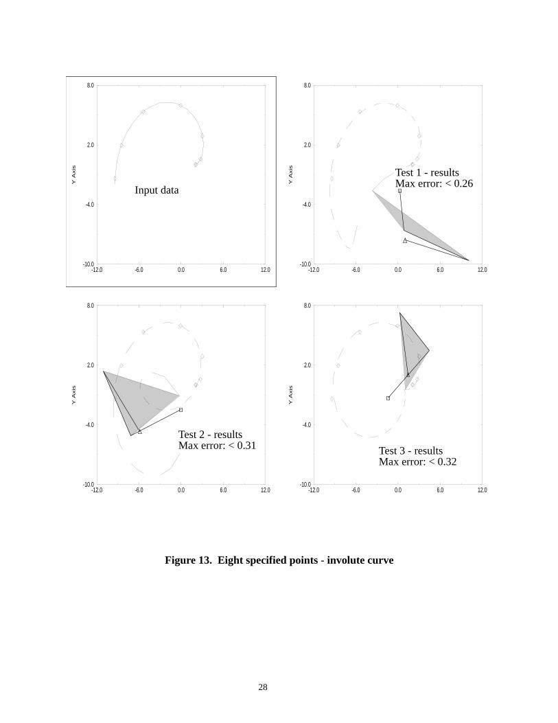
6.7 Eight specified points - involute curveBy specifying eight points, the coupler curves of these three mechanisms (in the region of interest)more closely approximate an involute curve than the coupler curves from the previous solutions,Figure 13. This suggests that by specifying a fairly large number of points, it may be possible tofind a four-bar mechanism that follows a particular path, (also see Section 6.10). Both drag-linkand crank-rocker mechanisms appear in these solutions.
6.8 Four specified points - straight line motionThe purpose of this test was to see if the GA method could produce one of the “classical” solutionsto straight-line motion generation using a four-bar mechanism, Figure 14. Test 1 failed to generatestraight-line motion, but properly generated a small error. The coupler curves generated for Tests2 and 3 are similar to the curves generated by the classical Chebyshev straight-line mechanism,although neither of these mechanisms bear much resemblance to it. These examples indicate theneed to use more points to achieve the straight line motion. This is done in the next experiment.This test also raises the as-yet unsolved question of translating functional objectives into the designdomain. The higher-level goal of this experiment is the generation of straight-line motion, bymeans of a mechanism that passes through a set of points. Since the former problem is notexpressed explicitly, the latter problem is solved instead, which can lead to undesirable results,such as those in Test 1.
6.9 Eleven specified points - straight line motionIncreasing the number of specified points from four to eleven greatly improves the quality of thecoupler curves, Figure 15. Since the length of the straight-line segment is 5, the path deviation per-cent error is about 2 percent. The shape of coupler curve from Tests 1, 2 and 3 are similar to thecoupler curve of the classical Chebyshev straight-line motion mechanism, but, as in the previousexperiment, these mechanisms do not resemble the classical ones. Test 2 results in an asymmetricvariant of Watt’s “grasshopper”. What makes the classical solutions so brilliant is that they weredeveloped from first principles without the aid of computers. What makes them special is they typ-ically have some special properties, such as symmetry. The GA method offers the opportunity fordiscovering many new classes of straight-line mechanisms, classes that may not share any of thesespecial properties with the classic solutions.
6.10 Twenty-four specified points - generated by four-bar
This experiment highlights one of the strengths of the GA synthesis method, the ability to specifythe entire coupler path, Figure 16. Classical techniques, or even the GA technique, may not suffi-ciently constrain the path of the coupler if too few points are specified. By specifying a largenumber of points, the path will necessarily be constrained. The results obtained by using the GAtechnique may yield “better” results than the classical (graphical) methods because, although theclassical methods will guarantee that the precision points are achieved exactly, the coupler pointpath from such a mechanism may not be viable for the particular application. With the GA method,although the specified points are not precisely achieved, the overall shape of the coupler point pathcan be guaranteed. Not only are all of the mechanisms shown crank-rockers, but they are muchmore similar to each other than the solutions presented in the previous experiments.
12
6.11 The need for scaling
The key point to note in this experiment is the small size of the input data coupler curve withrespect to the size of the space representable by the GA method, Figure 17. This curve occupies anarea of approximately 0.25 by 0.25, or about 0.01 percent of the area covered by the representablespace. Although the results from Test 1 are quite good, the results from Tests 2 and 3 show twosolutions with high fitness values, but whose solutions are probably not acceptable. This indicatesthe need to specify more points if a path is to be followed and also the need to scale the specifiedpoints (or the mechanism) so that the points occupy a larger percentage of the representable space.Scaling may be straightforward if only positional constraints are imposed. If velocity and/or accel-eration constraints are imposed, scaling may not be easy to implement.
6.12 Convergence and computational requirementsThis section examines two issues of concern when dealing with computational design methodolo-gies. The first is the rate at which the solution converges and the second is the computing resourcesrequired to achieve these solutions.
Figure 18 presents two plots that show the rate at which the problem converges. The first plotshows the maximum and average fitness as a function of generation. The large jumps in fitness aredue to the rescaling of the evaluation function, see Section 5. The second plot shows the minimumsum of the position errors and the average sum of the position errors. (Note that the minimum sumof the position errors values were multiplied by 100.)
There are two control parameters that strongly effect the run-time of this algorithm, and twothat weakly affect it. The two that strongly effect the run-time are the population and the numberof generations. For each of these parameters, the change in run-time should be a linear function ofthe change in the parameter. For example, doubling any one of these should result in a doubling ofthe run-time. The parameters that weakly effect run-time are the required input rotation and thenumber of specified points. The effect of the required input rotation parameter is unclear: Specify-ing a larger value means that more points will be compared, although some mechanisms will notbe checked because they will fail to meet the requirement. However, a smaller value for this param-eter means that more mechanisms will be checked. Overall, a larger parameter value will probablyincrease run-time, but the relationship is not clear. The number of specified points do not have asignificant impact on the execution time, since the most computationally expensive part of theexperiment is the mechanism synthesis. Doubling the number of specified points has little impacton the overall time.
Table 3 presents some run-time results from running this program. These results wereobtained on a Sparc 20/61TGX with 32 MB of memory. All parameters are the same as shown inTable 2, except as superceded here. Each entry shows the average time and standard deviation, inseconds, for three runs. These times were obtained by using the Unix /usr/bin/time routine.Each time was obtained by running each experiment three times and averaging the results:
Table 3 shows that the times do not scale exactly linearly with population or generations, butthis is expected since creating the first generation requires some fixed amount of time. The averagetime (and standard deviation) required to generate a population of 100, 200 and 300 mechanismsis 16.4 (2.1), 32.8 (1.4) and 50.6 (2.68) seconds respectively. Not only do these times agree withthe claim that the size of the population has a linear affect on the execution time, but subtracting
13
these times from the times shown in Table 3, makes those values more closely agree with the claim.For example, with a population of 200 and four specified points, the ratio of the times for 100 and150 generations to 50 generations is 1.75:1 and 2.58:1. However, subtracting the time to generatethe population changes the ratios to 1.95:1 and 3.01:1. Thus, the claim is well supported and canbe used by the designer to estimate the computing resources necessary to solve a specified problem.
7 Future workThere are four main directions for future work: GA parameter determination, parallel processorimplementations of the algorithm, a method for automatically scaling the representation and pack-ing the algorithm into a user-friendly tool.
As indicated in Section 6, the control parameters for these experiments were not selectedaccording to a methodology, rather, values reported by others to have worked were used, Goldberg(1989a). One of the strengths of the GA approach is that once formulated as a GA problem, thesolution methodology is the same for all problems. Thus, control parameters that have been dem-onstrated to work in other problems can be applied here, although the problem domains aredifferent, with the expectation that these control parameters will yield reasonable results. Research-ers have also done some preliminary work in defining optimium control parameters, such aspopulation size, see Goldberg (1989b). Experimentation within the specific problem domain canlead to modifications of the base set of control parameters to yield better results within that domain.
A better way to select the control parameters might be to create a meta-GA, that is, a GAwhose genome is comprised of the control parameters to the four-bar synthesis procedure andwhose evaluation function is an instantiation of the four-bar synthesis procedure. There are fourdifficulties with this approach: first, the computation resources required would be prodigious.Assuming that the control parameters can be coded into a 32 bit string, a population of at least 50individuals for a minimum of 20 generations would be required. Based on results presented inTable 3, we estimate 75 hours of CPU time on a Sparc 20. Second, to minimize the effect of theinitial random seed, each meta-GA genome would have to be executed several times so an averagefitness, independent of the initial random seed, could be calculated. If each genome is tested fourtimes, this could potentially increase the computing time to 300 hours. Third, it is possible that theparameter set developed to solve one particular problem may not be the ideal set for solvinganother problem. There is no way to determine this without running a meta-GA for the new prob-lem. Furthermore, even if a set of parameters is found to work well for two problems, that is not aguarantee that it will work well for all problems. Fourth, what parameters should be used to controlthe meta-GA? The parameter estimation problem is not closed, but recurses to a higher level.
An area of active research in GA theory development is parallel processor implementation.For problems with calculation-intensive evaluation functions, such as mechanism analysis, suchimplementations are necessary for general acceptance. The evaluation function for a typical GAproblem may consume 70-80% of the total CPU time. For the four-bar synthesis problem, the eval-uation function consumes in excess of 96% of the total CPU time. Since the evaluation of theindividuals mechanisms can be carried out in parallel, the total run time might be reduced by a fac-tor as large as the size of the population. With such reductions in run-time, this methodologybecomes practical for commercial applications. Such a reduction in run time also enables theimplementation of a meta-GA, as previously discussed.
14
As suggested in Section 5 and as demonstrated in Section 6.11, the method as currentlyimplemented may fail to find appropriate solutions for reasons related to scaling. The proceduremay also fail to find solutions because the solutions falls outside the representational space of theimplementation being used. To overcome these difficulties, a technique is needed that can changethe meaning of the representation in process. For the example shown in Section 6.11, a better rep-resentation may be to represent smaller mechanisms whose base points are closer to the desiredcoupler path.
Finally, to be of practical value, this methodology should be incorporated into a user-friendlytool. Such a tool should have a graphical interface that allows the user to pick the specified points,animate the generated mechanisms and allows the user to manually modify the mechanisms param-eters to observe the results of those changes.
8 ConclusionsThe results of the experiments indicate that the evaluation function proposed, Equation (5), can beused to generate four-bar mechanisms using a GA approach. The concern raised about scaling,Section 6.11, is a concern for any optimization based synthesis technique and must be addressedfurther. The applicability of other optimization techniques for solving this problem is not addressedin this paper. Other optimization techniques that require auxiliary information, such as local gradi-ents, may not work well on this problem because certain small parameters changes can dramaticallyalter the mechanism’s performance. However, combining a hill-climbing technique with the GAmay provide better results than those shown here. With a technique based on a combination of GAand hill-climbing, the GA would be used to rapidly get a “coarse” answer, then the hill-climbingtechnique would refine that answer.
The GA methodology utilized is domain independent and does not have any specific knowl-edge of the problem domain, i.e., the methodology is independent of the problem being solved.Thus, by demonstrating the correctness of the GA methodology, we can then apply it to solve avariety of engineering problems. A more advanced formulation of this methodology has the capa-bility of carrying out the simultaneous type, number and dimension synthesis for general planarmechanisms, Roston (1994).
9 BibliographyGoldberg, David E. (1989a), Genetic Algorithms in Search, Optimization and Machine Learning.
Addison-Wesley Publishing Company, Reading, MA.
Goldberg, David E. (1989b), Sizing populations for serial and parallel genetic algorithms. In Pro-ceedings of the 3rd International Conference on Genetic Algorithms, George Mason Univer-sity.
Hain, Kurt. (1967), Applied Kinematics. McGraw Hill, New York.
Hartenberg, Richard S.and Denavit, Jacques. (1964), Kinematic Synthesis of Linkages. McGraw-Hill Book Company, New York.
Holland, John H. (1975), Adaptation in Natural and Artificial Systems. MIT Press, Cambridge,MA.
15
Hrones, John A. and Larsen, George L. (1951), Analysis of the four-bar linkage; its application tothe synthesis of mechanisms. John Wiley & Sons, New York.
De Jong, K.A. and Spears, (1992), W.M. A formal analysis of the role of multi-point crossover ingenetic algorithms. Annals of Mathematics and Artificial Intelligence, 5(1), 1-26.
Roston, Gerald P. (1994), On the Genetic Design of Real-World Systems. Ph.D. thesis, CarnegieMellon University. (Available as CMU-TR-RI-94-42.)
Roston, G. and Sturges, R. (1995), A Genetic Design Methodology for Stucture Configuration. InProc. ASME Advances in Design Automation, Boston, MA, 1995.
Sandor, George N. and Erdman, Arthur G. (1977), Advanced Mechanism Design: Analysis andSynthesis, Volume 2. Prentice-Hall, Inc., Englewood Cliffs, NJ.
Shigley, Joseph E. (1977), Mechanical Engineering Design. McGraw Hill Book Company, NewYork.
Shigley, Joseph E. and Uicker, John J. (1980) Theory of Machines and Mechanisms. McGraw HillBook Company, New York.
16
procedure geneticAlgorithmbegin
initialize Population (t=0)evaluate Individuals in Population (t)while termination_conditions not satisfied, dobegin
t = t + 1select Population (t) from Population (t-1)recombine Individuals in Population (t)evaluate Individuals in Population (t)
endend
Figure 1. Psuedo-code representation of the genetic algorithm procedure