30
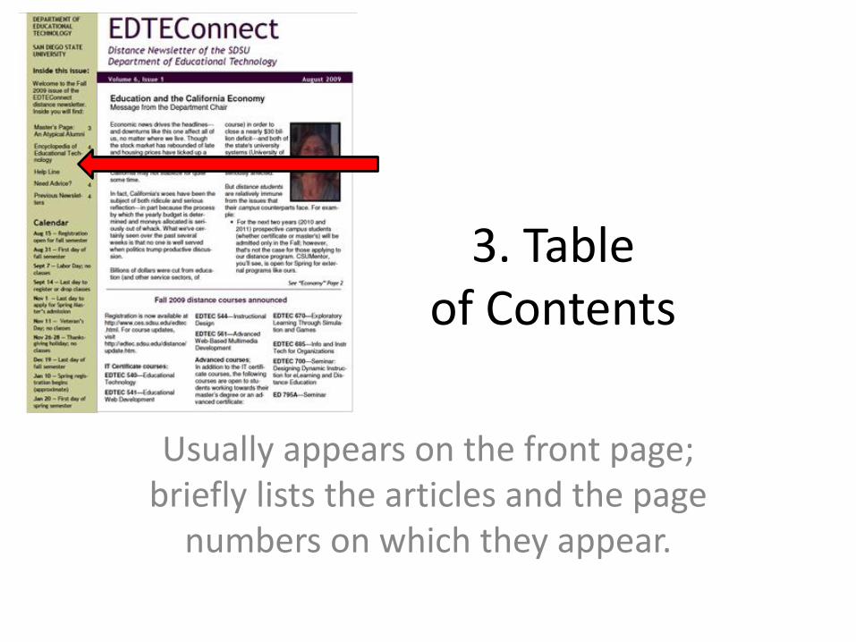
1.03 DTP Design Features: 12 Parts of a Newsletter Source: http://desktoppub.about.com/od/newsletters/a/newsletter_part.htm

0.5
setg
ray0
0.5
setg
ray1
Genetic Algorithms and GeneticProgramming
Pavia University and INFNSecond Lecture
Eric W. [email protected]
Vanderbilt University
Eric Vaandering – Genetic Programming, # 2 – p. 1/47

Course Outline• Machine learning techniques• Genetic Algorithms
• Review• Genetic Programming
• Basic concepts and differences from GeneticAlgorithms
• Genetic operators for Genetic Programming• Example• Generating constants• Applications
Eric Vaandering – Genetic Programming, # 2 – p. 2/47

Review of Genetic AlgorithmsLet’s recall the key points of what we learned last time:
• Genotype to phenotype matching• (Binary) string codes to model in determined way
• Subsequent generation created from previous generationaccording to biological models• Cloning• Crossover (sexual recombination)• Mutation
• Each individual has a fitness• Which individuals reproduce determined by fitness relative
to others• All choices are made randomly
Eric Vaandering – Genetic Programming, # 2 – p. 3/47

Genetic ProgrammingAlmost all of what we learned with Genetic Algorithms can beapplied to genetic programs. But, instead of evolving a genotype(a binary string) which maps to a phenotype (a predeterminedmodel) we will directly evolve the phenotype (a computerprogram). This program will (we hope) solve the problem wepose. Remember our supposition from last time:
Since we will use computer programs to implement oursolutions, maybe the form of our solution should be a
computer program.
This has the advantage of not specifying, in advance, the formour solution will take.
Eric Vaandering – Genetic Programming, # 2 – p. 4/47

Genetic Programming“How can computers learn to solve problems without beingexplicitly programmed? In other words, how can computers bemade to do what is needed to be done, without being told exactlyhow to do it?”
— Attributed to Arthur Samuel, 1959(Pioneer of Artificial Intelligence,coined term “machine learning”)
“Genetic programming is automatic programming. For the firsttime since the idea of automatic programming was first discussedin the late 40’s and early 50’s, we have a set of non-trivial,non-tailored, computer-generated programs that satisfy Samuel’sexhortation: ‘Tell the computer what to do, not how to do it.’ ”
— John Holland, University of Michigan, 1997(Pioneer of Genetic Algorithms)
Eric Vaandering – Genetic Programming, # 2 – p. 5/47

Programming AssumptionsWhen we normally program, we assume a number of guidelines:
• Correctness: The solution works perfectly• Consistency: The problem has one preferred solution• Justifiability: It is apparent why the solution works• Certainty: A solution exists• Orderliness: The solution proceeds in a orderly way• Brevity: Every part of the solution is necessary, a shorter
solution is better (Occam’s Razor)• Decisiveness: We know when the solution is complete
Genetic Programming requires that all ofthese assumptions be discarded
Eric Vaandering – Genetic Programming, # 2 – p. 6/47
GP principlesIn fact, in Genetic Programming:
• Correctness: A solution may be “good enough”• Consistency: Many very different solutions may be found• Justifiability: It may be very unclear how or why a solution
works• Certainty: A perfect solution may never be found• Orderliness: A solution may be very disorganized• Brevity: Large parts of the solution may do nothing• Decisiveness: We may never know if the best solution has
been found
Eric Vaandering – Genetic Programming, # 2 – p. 7/47

GP RepresentationsIn Genetic programming, instead of a binary string, we build,mutate, and cross-over programs. Internally, this is often (at leastoriginally) done in LISP because these types of operations areeasy in LISP’s representation (everything is a function).
Let’s look at a simple function:
C code: LISP Code:
float myfunc(float x, float y) {float val;if (x > y) {
val = x*x + y;} else {
val = y*y + x;}return val;
}
(IF (> x y)(+ (* x x) y)(+ (* y y) x)
)
Eric Vaandering – Genetic Programming, # 2 – p. 8/47

Tree RepresentationGP operations are even easier to illustrate if we adopt a “Tree”representation of a program. In this representation our examplebecomes:
C code: Program tree
float myfunc(float x, float y) {float val;if (x > y) {
val = x*x + y;} else {
val = y*y + x;}return val;
}
IF
>
x y
+
*
x x
y
+
*
y y
x
Eric Vaandering – Genetic Programming, # 2 – p. 9/47

Tree Representation, cont.From a fraction of our tree, we can see a few things:
+
*
x x
y
Two kinds of “nodes”• There are functions (IF, >, +, ∗)• There are “terminals” (x, y)• A function can have any number of
arguments (IF has three, sin x hasone)
If we allow any function or terminal at any position, then alloperations must be allowed:
• IF (float)• x + (y > x)
• Divide by zero (if we use division)
Eric Vaandering – Genetic Programming, # 2 – p. 10/47

Prepatory StepsIn the Genetic Algorithm, we began by defining a representation.(A binary string that mapped to the “physical” model).
In Genetic programming, we do something a little different. Wechoose a set of terminals (variables, for instance) and a set offunctions (which take these variables as parameters). These“atoms” or “nodes” will form the basis of our programs(solutions).
As in the Genetic Algorithm, we have to define the fitness of aprogram for solving the problem.
Eric Vaandering – Genetic Programming, # 2 – p. 11/47

Building a treeTrees are randomly built up one node at a time.
IF Root node ’IF’ has 3 args.
Eric Vaandering – Genetic Programming, # 2 – p. 12/47

Building a treeTrees are randomly built up one node at a time.
IF
>
Root node ’IF’ has 3 args.’>’ chosen for 1st arg.
Eric Vaandering – Genetic Programming, # 2 – p. 13/47

Building a treeTrees are randomly built up one node at a time.
IF
>
x y
Root node ’IF’ has 3 args.’>’ chosen for 1st arg.x and y terminate ’>’
Eric Vaandering – Genetic Programming, # 2 – p. 14/47

Building a treeTrees are randomly built up one node at a time.
IF
>
x y
+
*
Root node ’IF’ has 3 args.’>’ chosen for 1st arg.x and y terminate ’>’Next branch started
Eric Vaandering – Genetic Programming, # 2 – p. 15/47

Building a treeTrees are randomly built up one node at a time.
IF
>
x y
+
*
x x
y
+
* x
Root node ’IF’ has 3 args.’>’ chosen for 1st arg.x and y terminate ’>’Next branch startedFinal branch started
Eric Vaandering – Genetic Programming, # 2 – p. 16/47

Building a treeTrees are randomly built up one node at a time.
IF
>
x y
+
*
x x
y
+
*
y y
x
Root node ’IF’ has 3 args.’>’ chosen for 1st arg.x and y terminate ’>’Next branch startedFinal branch startedTree is complete(all branches terminated)
Eric Vaandering – Genetic Programming, # 2 – p. 17/47

CrossoverRecall in GA, crossover was a swap of DNA at a chosen point.Here’s how we do crossover in GP:
+
×
x x
y
+
y −
y x
Pick two parents
Eric Vaandering – Genetic Programming, # 2 – p. 18/47

CrossoverRecall in GA, crossover was a swap of DNA at a chosen point.Here’s how we do crossover in GP:
+
×
x x
y
+
y −
y x
Pick two parentsPick break point on each
Eric Vaandering – Genetic Programming, # 2 – p. 19/47

CrossoverRecall in GA, crossover was a swap of DNA at a chosen point.Here’s how we do crossover in GP:
+
×
x −
y x
y
+
y x
Pick two parentsPick break point on eachSwap sub-trees
Eric Vaandering – Genetic Programming, # 2 – p. 20/47

CrossoverRecall in GA, crossover was a swap of DNA at a chosen point.Here’s how we do crossover in GP:
+
×
x −
y x
y
+
y x
Pick two parentsPick break point on eachSwap sub-trees
We have two new indi-viduals for our next gen-eration
Eric Vaandering – Genetic Programming, # 2 – p. 21/47

MutationIn GA, mutation was a bit flip at a single location.Here’s how mutation works in GP:
+
×
x x
−
y y
Pick a parent
Eric Vaandering – Genetic Programming, # 2 – p. 22/47

MutationIn GA, mutation was a bit flip at a single location.Here’s how mutation works in GP:
+
×
x x
−
y y
Pick a parentPick a mutation point
Eric Vaandering – Genetic Programming, # 2 – p. 23/47

MutationIn GA, mutation was a bit flip at a single location.Here’s how mutation works in GP:
+
×
x x
Pick a parentPick a mutation pointRemove the subtree
Eric Vaandering – Genetic Programming, # 2 – p. 24/47

MutationIn GA, mutation was a bit flip at a single location.Here’s how mutation works in GP:
+
×
x x
−
x
Pick a parentPick a mutation pointRemove the subtreeStart a new subtree
Eric Vaandering – Genetic Programming, # 2 – p. 25/47

MutationIn GA, mutation was a bit flip at a single location.Here’s how mutation works in GP:
+
×
x x
−
x +
y x
Pick a parentPick a mutation pointRemove the subtreeStart a new subtree
Finish the new subtree just asif it were a “root” tree
Mutation can often be very destructive in Genetic Programming(as opposed to bit-flips in GA).As in GA, both crossover and mutation are random processes.
Eric Vaandering – Genetic Programming, # 2 – p. 26/47

Practical considerationsObviously, a tree can grow nearly infinite in size. This is usuallyundesirable. There are ways to control this:
• Set limits on number of nodes• Set limits on depth of nodes• Create initial topologies of specified depth
A common approach is to allow half of the initial population togrow completely randomly and to create the other half at a rangeof (shallow) depths. In the latter case, pick functions for all nodes< desired depth, pick terminals for all nodes at desired depth.
Eric Vaandering – Genetic Programming, # 2 – p. 27/47

RepresentationsIn the simplest form of tree representation, input values andoutput values must be of the same type.
• Have to assume a representation when mixing type offunctions• Logical and real? Maybe > 0 is TRUE (1)
• Must protect against divide-by-zero,√
< 0, log(< 0), etc.• Type needn’t be simple (integer, float, etc.). Can be any
“object.”
There are also representations of GP which are not “tree”representations. There are also strongly-type representations.
Eric Vaandering – Genetic Programming, # 2 – p. 28/47

Genetic Programming ExampleLet’s take a look at an example of a simple GeneticProgramming excercise. This example is taken from
http://www.genetic-programming.com/gpquadraticexample.htmlwhich goes into more detail.The goal: create a computer program which outputs the samevalues as x2 + x + 1 over the interval (−1,+1)
Notice the goal is not to create a program that is explicitlyx2 + x + 1. (Remember the 7 assumptions of programming wehad to discard.)
Eric Vaandering – Genetic Programming, # 2 – p. 29/47

GP Example SetupDefine functions:
We’ll keep this simple and pick +, −, ×, and /.Remember / has to work for all values, so x/0 ≡ 1.
Define terminals:We want the variable x, of course.Also put in integers from (−5,+5).
Define fitness:In theory, we’d like to use the integral of the area (absolute
value) between the program and x2 + x + 1 from (−1,+1)In practice, we’ll do this numerically for maybe 100 points
Termination criterion:Require the fitness of best individual < 0.01
With these few definitions, we are ready to run.
Eric Vaandering – Genetic Programming, # 2 – p. 30/47

GP Example, Generation 0In our simple example, we will generate just 4 programs:
−
+
x 1
0
+
1 ×
x x
+
2 0
×
x −
−1 −2
x + 1 x2 + 1 2 x
These are our four starting trees and their algebraic equivalents.
Eric Vaandering – Genetic Programming, # 2 – p. 31/47

Generation 0 FitnessNow let’s look at the four examples in our population
x + 1 x2 + 1 2 x
Here are the four programs from the previous slide and theirdifferences from x2 + x + 1 shown graphically. (The difference,or fitness, is the area of the gray curve.)
x2 + 1 and x + 1 have the lowest (best) fitness.
As expected, randomly generated programs will not usually bevery efficient at solving even the simplest problems. But, somewill be better than others.
Eric Vaandering – Genetic Programming, # 2 – p. 32/47

GP Example, Generation 1Now it’s time to “breed” a new generation of programs.
• Usually ∼ 90% crossover, ∼ 10% cloning, ∼ 1% mutation• Our next generation: 2 crossover children, 1 clone, 1
mutation
First the clone, which happens to be the program with the bestfitness (likely to participate, but not necessarily as a clone).
−
+
x 1
0
Eric Vaandering – Genetic Programming, # 2 – p. 33/47

Generation 1, MutationLet’s assume the 3rd tree is chosen for mutation:
+
2 0
Location of “2” is randomlychosen for mutation and isremoved.
+
/
x x
0A new tree (x/x with protec-tion) is inserted in its place.
Eric Vaandering – Genetic Programming, # 2 – p. 34/47

Generation 1, CrossoverLastly, two programs are chosen for crossover giving two newprograms:
−
+
x 1
0
+
1 ×
x x
→
−
x 0
+
1 ×
+
x 1
x
Eric Vaandering – Genetic Programming, # 2 – p. 35/47

GP Example, Generation 1Here are our four trees for Generation 1
−
+
x 1
0
+
/
x x
0
−
x 0
+
1 ×
+
x 1
x
x + 1 1 x x2 + x + 1
The final program is the perfect solution; the run is ended.
Eric Vaandering – Genetic Programming, # 2 – p. 36/47

Generation 1, CrossoverFirst, let’s look at the best solution and why finding it is notcompletely random. It is the combination of two good traits fromits two parents (who were “better” programs than theirneighbors).
−
+
x 1
0
+
1 ×
x x
→
+
1 ×
+
x 1
x
Of course, the computer had no way of knowing which traitswere good, just which individuals had them.
Eric Vaandering – Genetic Programming, # 2 – p. 37/47

GP Example, ContinuedAlso, our simple example illustrates a few other points:
• Brevity: Many of the programs in our example could besimplified:
+
/
x x
0
• 1st individual from generation 0 picked twice, 4th not picked(lowest fitness)
• But, a perfect solution has been found, which is notguaranteed in Genetic Programming
Eric Vaandering – Genetic Programming, # 2 – p. 38/47

Further pointsOk, so finding a program to “fit” x2 + x + 1 was easy. What ifour target function was 2.718x2 + 3.1416x or something similar?
There are two ways Genetic Programs accomplish this, oneimplicit, one explicit:
• The GP can manufacture constants from functions andoperators
• Introduce the concept of an ephemeral random constant(ERC). This is function that when first called, returns arandom number. Thereafter, it returns the same number. Weadd this to our set of terminals. We denote this in ourterminal set by R.
We’ll look at both of these cases.
Eric Vaandering – Genetic Programming, # 2 – p. 39/47

Implicit Constant GenerationLet’s look for a function that is equal to cos 2x where x rangesfrom 0 to 2π. (Example from Koza, Vol. I).
For terminals, we choose [x, 1.0, 2.0]. For functions, +, −, ×, /,and sin. (We leave out cos to avoid trivial solutions).
In generation 30 of such a run, whatwas found was this:Where “Const” is a generated constantdefined on the next page.This simplifies to sin(2−Const− 2x).
sin
−
−
2 ×
2 x
Const
Eric Vaandering – Genetic Programming, # 2 – p. 40/47

Implicit Constant Generation
The constant that is evolved is this:
This expression evaluates to 0.433, sosin(2−Const−2x) becomes sin(1.567−2x).π/2 = 1.571.
The identity “discovered” is
sin(π
2− 2x) = cos 2x.
sin
sin
sin
sin
sin
sin
×
sin
sin
1
sin
sin
1
Eric Vaandering – Genetic Programming, # 2 – p. 41/47

Implicit Constant GenerationHow did this happen?
• Constant evolved over time• First, sin 1.0 = 0.841
• Then, sin(sin 1.0) = 0.746
• Then, sin2(sin 1.0) = 0.556
• Then, successive applications of sin(x) to give 0.528,0.504, 0.483, 0.464, 0.448, 0.433
Eric Vaandering – Genetic Programming, # 2 – p. 42/47

Explicit Constant GenerationWe can also introduce the concept of an ephemeral randomconstant (ERC). This is function that when first called, returns arandom number. Thereafter, it returns the same number. We addthis to our set of terminals. We denote this in our terminal set byR.
This gives the GP a group of constants which can be combined tocreate new constants.
For instance, let’s return to the problem of evolving2.718x2 + 3.1416x with terminals of x and R.
Eric Vaandering – Genetic Programming, # 2 – p. 43/47

Explicit Constant GenerationAfter 41 generations, we can evolve the tree:
+
−
+
×
-0.50677 x
+
×
-0.50677 x
×
-0.76526 x
×
+
0.11737 x
+
−
x ×
-0.76526 x
x
Eric Vaandering – Genetic Programming, # 2 – p. 44/47

Explicit Constant GenerationThis tree simplifies to the form 2.76x2 + 3.15x.
Recall we were looking for 2.72x2 + 3.14x.
Final point: The examples we’ve shown involve functions thatreturn a single number. This need not be the case. If yourframework is in C, your return value can be a structure. In C++ itcan be an object. If you want, you can even generate programs inassembly code or even high level languages. The simplestmodels follow this function-tree representation, but fullyspecified grammars are possible with existing software.
Eric Vaandering – Genetic Programming, # 2 – p. 45/47

GP ApplicationsWe can see that this might be applicable to a wide variety ofapplications. Here are some proven examples:
• Symbolic regression (finding a functional form for a set ofdata)
• Determining which combinations of 10,000 genes causecancer
• A filter to classify high energy physics events
This last example is the use I’ve been studying, so we’ll look at itin more detail next time.
Eric Vaandering – Genetic Programming, # 2 – p. 46/47

GA & GP ResourcesThere is a lot of information on the web about GeneticAlgorithms and Programming:
• http://www.aic.nrl.navy.mil/galist/ —Genetic Algorithms
• http://www.genetic-programming.org/ —John Koza
Software frameworks for both GA and GP exist in almost everylanguage (most have several)
• http://www.genetic-programming.com/coursemainpage.html#_Sources_of_Software
• http://zhar.net/gnu-linux/howto/ – GNU AIHowTo (GA/GP/Neural nets, etc.)
• http://www.grammatical-evolution.org —GA–GP Translator
Eric Vaandering – Genetic Programming, # 2 – p. 47/47


