PNNL-14584, Rev. 4

GENII Version 2 Software Design Document B. A. Napier D.L. Strenge J.V. Ramsdell, Jr. P.W. Eslinger C. Fosmire September 2012 Prepared under Contract DE-AC05-76RLO 1830

DISCLAIMER

This report was prepared as an account of work sponsored by an agency of the United States Government. Neither the United States Government nor any agency thereof, nor Battelle Memorial Institute, nor any of their employees, makes any warranty, expressed or implied, or assumes any legal liability or responsibility for the accuracy, completeness, or usefulness of any information, apparatus, product, or process disclosed, or represents that its use would not infringe privately owned rights. Reference herein to any specific commercial product, process, or service by trade name, trademark, manufacturer, or otherwise does not necessarily constitute or imply its endorsement, recommendation, or favoring by the United States Government or any agency thereof, or Battelle Memorial Institute. The views and opinions of authors expressed herein do not necessarily state or reflect those of the United States Government or any agency thereof.

PACIFIC NORTHWEST NATIONAL LABORATORY

operated by BATTELLE MEMORIAL INSTITUTE

for the UNITED STATES DEPARTMENT OF ENERGY

under Contract DE-AC05-76RLO 1830

Printed in the United States of America

Available to DOE and DOE contractors from the Office of Scientific and Technical Information, P.O. Box 62, Oak Ridge, TN 37831;

prices available from (615) 576-8401.

Available to the public from the National Technical Information Service, U.S. Department of Commerce, 5285 Port Royal Rd., Springfield, VA 22161

SOFTWARE DESIGN DESCRIPTION Contents 1 Introduction ......................................................................................................................1 1.1 Purpose ...............................................................................................................1 1.2 Scope ..................................................................................................................1 1.3 Framework Operating Structure .........................................................................2 1.4 Definitions and Acronyms ..................................................................................2 1.5 References for Section 1 .....................................................................................5 2 Software Structure ...........................................................................................................7 2.1 Framework User Interface (FUI) ........................................................................8 2.2 Primary Data Communication Files (PDCF) .....................................................8 2.3 Sensitivity User Interface (SUI) .......................................................................10 2.4 GENII-V2 Calculational Modules ...................................................................10 2.4.1 GENII-V2 Source Term Definition Module .....................................10 2.4.2 GENII-V2 Surface Water Transport Module ....................................11 2.4.3 GENII-V2 Atmospheric Transport Modules .....................................11 2.4.4 GENII-V2 Exposure Pathways Modules ..........................................11 2.4.4.1 GENII-V2 Near-field Exposure Module ..............................12 2.4.4.2 GENII-V2 Acute Exposure Module .....................................12 2.4.4.3 GENII-V2 Chronic Exposure Module ..................................12 2.4.5 GENII-V2 Receptor Intake Module ..................................................13 2.4.6 GENII-V2 Health Impact Module .....................................................13 2.4.7 GENII-V2 Report Generators ...........................................................13 2.4.8 GENII-V2 Biota Dose Module ...........................................................13 2.5 Global Input Data File ......................................................................................14 2.6 Auxiliary Data Input/Output Files ....................................................................14 2.7 References for Section 2 ...................................................................................14 3 Auxiliary Data Communication Files ............................................................................15 3.1 Auxiliary Data Communication File Summaries .............................................15 3.2 Radionuclide Master Data File .........................................................................15 3.3 Meteorological Data .........................................................................................15 3.4 Dosimetry/Risk Files ........................................................................................16

3.4.1 Radiation Dose Factor Index File ....................................................17 3.4.2 External Dose Rate Conversion Factor Files ...................................17 3.4.3 Internal Dose Conversion Factor Files ...........................................17 3.4.4 Risk Conversion Factor Files ...........................................................18

3.5 Radon output file ..............................................................................................18 3.6 References for Section 3 ...................................................................................18 4 Sensitivity User Interface ...............................................................................................20 4.1 Structure and Interface .....................................................................................20 4.2 Mathematical Strategies for Generating Random Variables ............................20

4.2.1 Probability Concepts for Univariate Random Number Generation .........................................................................................20

4.2.1.1 Random Number Generation by the Probability Integral Transform Method .................................................21

4.2.1.2 Dependence on the Uniform Random Number Generator .............................................................................22

4.2.2 Latin Hypercube Sampling ................................................................22 4.2.2.1 Stratified Sampling ..............................................................22 4.2.2.2 Imposing Rank Correlations ................................................23 4.2.2.3 Insuring a Positive-Definite of Correlation Matrix ...............25 4.2.2.3.1 Obtaining Eigenvalues and Eigenvectors ...............25 4.2.2.3.2 Adjusting the Correlation Matrix ...........................26 4.2.3 Statistical Distributions .....................................................................26 4.2.3.1 Algorithms for the Uniform Distribution .............................26 4.2.3.1.1 Generation Algorithm .............................................28 4.2.3.1.1.1 Uniform (0,1) Generator ...........................28 4.2.3.1.1.2 Uniform (a,b) Generator ...........................28 4.2.3.2 Algorithm for the Loguniform Distribution .........................29 4.2.3.2.1 Definition of the PDF .............................................29 4.2.3.2.2 CDF and Inverse CDF Algorithms .........................29 4.2.3.3 Algorithms for the Normal Distribution ..............................29 4.2.3.3.1 Definition of the PDF .............................................29 4.2.3.3.2 CDF Algorithm .......................................................30 4.2.3.3.3 Inverse CDF Algorithm ..........................................30 4.2.3.3.4 Precision .................................................................31 4.2.3.4 Algorithm for the Lognormal Distribution ..........................31 4.2.3.4.1 Definition of the PDF .............................................32 4.2.3.4.2 Generation Algorithms ...........................................32 4.2.3.4.3 Precision .................................................................32 4.2.3.5 User-Specified Distribution .................................................33 4.3 Uncertainty Analysis Methods .........................................................................33 4.3.1 CDF's and CCDF's ............................................................................33

4.3.2 Sample Mean, Quantiles and their Corresponding Confidence Limits ................................................................................................34

4.3.2.1 Sample Mean and Confidence Limits ..................................34 4.3.2.2 Sample Quantile and Confidence Limits .............................35 4.4 References For Section 4 ..................................................................................36 5 Atmospheric Transport and Deposition Modules ..........................................................38 5.1 Straight-Line Gaussian Plume Model ...............................................................38

5.1.1 Basic Model .....................................................................................38 5.1.2 Sector-Average Model .....................................................................40 5.1.3 Area Source Model ..........................................................................41

5.1.3.1 Centerline Area Model ......................................................41 5.1.3.2 Sector-Averaged Area Model ...........................................42

5.1.4 Finite Source Correction ...................................................................43

5.1.5 Multiple Sources ................................................................................44 5.1.6 Calm Winds .......................................................................................46 5.1.7 Calculation Of Average And Time Integrated Concentrations .........46 5.2 Lagrangian Puff Model .....................................................................................46 5.2.1 Transport ............................................................................................47 5.2.2 Puff Diffusion ....................................................................................48 5.2.3 Calculation Of Concentrations And Exposure ..................................50 5.2.4 Sector-Average Model ......................................................................50 5.2.5 Multiple Sources ................................................................................50 5.2.6 Area Sources ......................................................................................51 5.2.7 Calm Winds .......................................................................................51 5.2.8 Finite Sources....................................................................................51 5.3 Model Component Parameterizations ..............................................................51 5.3.1 Effective Release Height ...................................................................51 5.3.1.1 Downwash Correction .........................................................52 5.3.1.2 Plume Rise ...........................................................................52 5.3.2 Wind Profile ......................................................................................57 5.3.3 Dispersion coefficients ......................................................................59 5.3.4 Dispersion coefficient Corrections ....................................................67 5.3.4.1 Building Wakes And Low Wind Speed Meander ................67 5.3.4.2 Buoyancy Induced Diffusion ...............................................72 5.3.5 Deposition .........................................................................................73 5.3.5.1 Dry Deposition .....................................................................73 5.3.5.2 Wet Deposition ....................................................................75 5.3.5.3 Total Deposition ...................................................................77 5.3.6 Radioactive Decay ............................................................................78 5.3.7 Depletion ...........................................................................................79 5.4 Finite Plume Submersion Dose ........................................................................83 5.4.1 Puff Model Cloud-Shine Dose Calculation .......................................83 5.4.2 Plume Model Cloud-Shine Dose Calculation ...................................86 5.4 Atmospheric Data ............................................................................................88 5.5 References for Section 5 ...................................................................................89 6 Surface Water Transport Module ...................................................................................93 6.1 River Transport Models ..................................................................................93

6.2 Near-Shore Lake Transport Models ...............................................................95 6.3 Impoundment Models .....................................................................................96 6.4 Radioactive Decay in Transit ..........................................................................98 6.5 References for Section 6 .................................................................................99

7 Near-Field Exposure Module .......................................................................................100 7.1 Communication Interfaces .............................................................................100 7.2 Source Configurations and Soil Model ..........................................................101 7.2.1 Method for Reconciliation of Activity Units ..................................104 7.2.2 Release Rate From Subsurface Waste Package ..............................105 7.2.3 Biotic Transfer to the Surface by Plants ..........................................105

7.2.4 Biotic Transfer to the Surface by Animals ......................................106 7.2.5 Leaching from the Surface Soil Zone ..............................................107 7.2.6 Loss by Harvest ...............................................................................107 7.2.7 Transfer by Redistribution ...............................................................108 7.2.8 Soil Model Application to Near-Field Exposure Module ...............108 7.3 External Exposure Pathways ..........................................................................109 7.2.1 External Air Immersion ...................................................................109 7.2.2 External Ground Exposure ..............................................................110 7.4 Ingestion Exposure Pathways .........................................................................110 7.3.1 Food Crop Ingestion ........................................................................112 7.3.2 Animal Product Ingestion ................................................................114 7.3.3 Inadvertent Soil Ingestion ...............................................................115 7.5 Inhalation Exposure Pathways .......................................................................116

7.4.1 Soil Suspension Air Inhalation .......................................................116 7.6 Special Models for Tritium and Carbon-14 ...................................................116 7.7 References for Section 7 .................................................................................117 8 Acute Exposure Module ..............................................................................................118

8.1 Communication Interfaces ............................................................................119 8.2 Soil Model .....................................................................................................120

8.2.1 Activity from Air and Water Deposition ........................................121 8.2.2 Leaching from the Surface Soil Zone .............................................122 8.2.3 Loss by Harvest...............................................................................122

8.3 External Exposure Pathways ..........................................................................123 8.3.1 External Plume Immersion ..............................................................123 8.3.2 External Groundshine Model ..........................................................124 8.3.3 External Exposure from Aquatic Recreational Activities ...............125 8.4 Acute Ingestion Exposure Pathways ..............................................................126 8.4.1 Terrestrial Food Ingestion ...............................................................126 8.4.2 Aquatic Food Ingestion ...................................................................133 8.4.3 Drinking Water Ingestion ................................................................134 8.4.4 Inadvertent Soil Ingestion ...............................................................135 8.5 Acute Inhalation Exposure Pathways .............................................................136 8.5.1 Inhalation of Airborne Contamination ............................................136 8.5.2 Inhalation of Resuspended Activity ................................................136 8.5.3 Inhalation of Indoor Contaminants from Water ..............................137 8.6 Special Radionuclide Models: Tritium and Carbon-14 ..................................138 8.7 References for Section 8 .................................................................................142 9 Chronic Exposure Module ...........................................................................................143 9.1 Communication Interfaces .............................................................................145

9.2 Soil Model ......................................................................................................146 9.2.1 Activity from Air and Water Deposition ..........................................147

9.2.2 Leaching from the Surface Soil Zone .............................................148 9.2.3 Loss by Harvest...............................................................................148

9.3 External Exposure Pathways ..........................................................................149

9.3.1 External Plume Immersion ..............................................................149 9.3.2 External Ground Exposure ..............................................................149 9.3.3 Recreational Swimming Immersion ................................................151 9.3.4 Recreational Boating Exposure .......................................................151 9.3.5 Recreational Shoreline Exposure ....................................................151 9.4 Ingestion Exposure Pathways .........................................................................152 9.4.1 Terrestrial Farm Product Ingestion ..................................................152 9.4.1.1 Terrestrial Media Concentrations ......................................153 9.4.1.2 Terrestrial Farm Crop Concentrations ...............................154 9.4.1.3 Terrestrial Farm Animal Product Concentrations ..............156 9.4.1.4 Interception Fraction ..........................................................158 9.4.1.5 Resuspension Factor ..........................................................160 9.4.1.6 Translocation Factor and Weathering Loss .......................160 9.4.2 Aquatic Food Ingestion ...................................................................160 9.4.3 Drinking Water Ingestion ................................................................161 9.4.4 Inadvertent soil Ingestion ................................................................161 9.5 Inhalation Exposure Pathways .......................................................................162 9.5.1 Inhalation of Air ..............................................................................162 9.5.2 Inhalation of Resuspended Soil .......................................................163 9.5.3 Indoor Inhalation of Waterborne Contaminants ..............................164 9.6 Special Radionuclide Models: Tritium and Carbon-14 ..................................165 9.6.1 Special Tritium Models ...................................................................166 9.6.2 Special Carbon-14 Models ..............................................................168 9.7 References for Section 9 ................................................................................171 10 Receptor Intake Module .............................................................................................173 10.1 Communication Interfaces ...........................................................................175 10.2 External Exposure Estimates ........................................................................175 10.2.1 External Plume Immersion ............................................................175 10.2.2 External Ground Exposure ............................................................176 10.2.3 Recreational Swimming Immersion ..............................................176 10.2.4 Recreational Boating Exposure .....................................................177 10.2.5 Recreational Shoreline Exposure ..................................................178 10.3 Ingestion Intake Estimates ............................................................................179 10.3.1 Terrestrial Farm Product Ingestion ................................................179 10.3.2 Aquatic Food Ingestion .................................................................180 10.3.3 Drinking Water Ingestion ..............................................................180 10.3.4 Inadvertent Soil Ingestion .............................................................181 10.3.5 Inadvertant Swimming Water Ingestion ........................................182 10.3.6 Inadvertant Shower Water Ingestion .............................................182 10.4 Inhalation Intake Estimates ..........................................................................183 10.4.1 Inhalation of Air ............................................................................183 10.4.2 Inhalation of Resuspended Soil .....................................................183 10.4.3 Indoor Inhalation of Contaminants Including Radon ....................184

11 Health Impact Module ...............................................................................................186 11.1 Communication Interfaces ...........................................................................186 11.2 Radiation Dose Assessment .........................................................................189 11.2.1 Federal Guidance Report Dosimetry .............................................189 11.2.2 Department of Energy Dosimetry .................................................189 11.2.3 Current ICRP Dose Coefficients ...................................................189 11.2.4 External Exposure Pathway Dose Assessment .............................190 11.2.5 Ingestion Exposure Pathway Dose Assessment ............................196 11.2.6 Inhalation Exposure Pathway Dose Assessment ...........................201 11.3 Health Risk Assessment ...............................................................................203 11.3.1 Use of Effective Dose ....................................................................203 11.3.2 Use of EPA Slope Factors .............................................................205 11.3.3 Use of Age- and Organ-dependent Risk Factors ...........................207 11.3.3.1 External Exposure Pathway Risk Assessment .................207 11.3.3.2 Ingestion Exposure Pathway Risk Assessment ...............210 11.3.3.3 Inhalation Exposure Pathway Risk Assessment ..............213 11.4 References for Section 11 .............................................................................214 12 Biota Dose Module ....................................................................................................217 12.1 Communication Interfaces ............................................................................218 12.2 Soil Model .....................................................................................................219 12.2.1 Activity from Air and Water Deposition ........................................220 12.2.2 Leaching from the Surface Soil Zone .............................................221 12.3 External Exposure Pathways .........................................................................221 12.3.1 Exernal Plume Immersion ..............................................................221 12.3.2 External Ground Exposure .............................................................222 12.3.3 Swimming Immersion ....................................................................223 12.3.4 Shoreline Exposure .........................................................................223 12.4 Terrestrial Biota Internal Contamination ......................................................224 12.4.1 Terrestrial Media Concentrations ...................................................225 12.4.2 Plant Concentrations .......................................................................226 12.4.3 Terrestrial Animal Concentrations .................................................227 12.4.3.1 Initial Interception Fraction ..............................................228 12.4.3.2 Resuspension Factor .........................................................229 12.4.3.3 Weathering Loss ...............................................................229 12.4.3.4 Soil Ingestion ....................................................................230 12.4.4 Aquatic Biota ..................................................................................230 12.5 Biota Dose Calculations ................................................................................231 12.5 References for Section 12 ..............................................................................232 Appendix A Primary Data Communication File Specifications ....................................234 Appendix B Auxiliary Data Communication File Specifications ................................260 Appendix C Radioactive Decay Processor ....................................................................268

Appendix D Transfer Factors .........................................................................................278 Appendix E Parameters Available for Stochastic Analysis ...........................................301 Appendix F Supplied Default Parameters .....................................................................310

1

1.0 INTRODUCTION This report describes the mathematical formulations and implementation structure for version 2 of the GENII software product (GENII-V2). The following sections define the purpose and scope of this report, the framework operating structure for GENII-V2, and definitions and acronyms used in this report. 1.1 PURPOSE The purpose of this document is to describe the architectural design for the GENII-V2 software package. This document defines details of the overall structure of the software, the major software components, their data file interfaces, and specific mathematical models to be used. The design represents a translation of the requirements (Napier et al. 1995) into a description of the software structure, software components, interfaces, and necessary data. The design focuses on the major components and data communication links that are key to the implementation of the software within the operating framework. The intended audience for this design report is the Pacific Northwest National Laboratory (PNNL) software development team, independent reviewers, testing team, users, and project and line management who need a thorough understanding of the software capabilities. 1.2 SCOPE The GENII-V2 software package has been developed for the Environmental Protection Agency, Office of Radiation and Indoor Air, with subsequent revisions for the US Department of Energy and US Nuclear Regulatory Commission. The software has two distinct user groups:

1) staff who will use the software frequently to perform analyses,

2) a large group of occasional users who may be required to perform analyses with the software.

All users are assumed to be competent in the areas of health physics and environmental analysis, with some basic familiarity with use of computers. The purpose of the GENII-V2 software package is to provide the capability to perform dose and risk assessments of environmental releases of radionuclides. The software also has the capability of calculating environmental accumulation and radiation doses from surface water, groundwater, and soil (buried waste) media when an input concentration of radionuclide in these media is provided. This report represents a detailed description of the capabilities of the software product with exact specifications of mathematical models that form the basis for the software implementation and testing efforts.

2

This report also presents a detailed description of the overall structure of the software package, details of main components (implemented in the current phase of work), details of data communication files, and content of basic output reports. 1.3 FRAMEWORK OPERATING STRUCTURE The components of GENII-V2 have been developed to operate within the Framework for Risk Analysis in Multimedia Environmental Systems (FRAMES). An overview of this software concept is provided by Whelan et al. (1997). FRAMES is an open-architecture, object-oriented system that allows the user to choose the most appropriate models to solve a particular simulation problem. The components of GENII-V2 are implemented through FRAMES by meeting requirements for data input and output file specifications defined for FRAMES. Details of FRAMES and implementation of the GENII-V2 components is described in Section 2. 1.4 DEFINITIONS AND ACRONYMS Definition of terms, acronyms, and abbreviations used in this report are defined below. Many of the technical term definitions are based on definitions provided in the glossary of Kennedy and Strenge (1992). Absorbed dose - The energy imparted by ionizing radiation per unit mass of irradiated material. The units of absorbed dose are the rad and the gray (Gy). Activity - The rate of disintegration (transformation) or decay of radioactive material. The units of activity are the curie (Ci) and the becquerel (Bq). Acute release - the release of material to the air or surface water over a brief period, assumed in the models to be on the order of a few hours. ASCII - American Standard Code for Information Interchange, a set of codes used in data communications. Bq - Abbreviation for becquerel, a unit of activity. Chronic release - a release of material to the air or surface water that continues essentially uniformly over a long period, taken in the models to be a year. Ci - Abbreviation for curie, a unit of activity. Class (or "lung class" or "inhalation class") - A classification scheme for inhaled material according to its rate of clearance form the pulmonary region of the lung. Materials are classified as F, M, or S (previously D, W, or Y), and apply to a range of clearance half-times for F (Fast) of less that 10 days, for M (Medium) from 10 to 100 days, and for S (Slow) of greater than 100 days.

3

Collective dose - The sum of the individual doses received in a given period of time by a specified population from exposure to a specified source of radiation. Committed dose equivalent (HT,50) - The equivalent dose to organs or tissues of reference (T) that will be received from an intake of radioactive material by an individual during the 50-year period following the intake. Committed effective dose equivalent (HE,50) - The sum of the products of the weighting factors applicable to each of the body organs or tissues that are irradiated by internally deposited radionuclides and the committed equivalent dose to these organs or tissues (HE,50 = wT HT,50) Database - A collection of logically organized information provided in support of a software program. Dose or "radiation dose" - A generic term that means absorbed dose, equivalent dose, effective dose, committed dose equivalent, or committed effective dose equivalent. Dose conversion factor - a precalculated multiplier that translates activity ingested or inhaled into absorbed dose, equivalent dose, or effective dose. Dose equivalent - see Equivalent dose. Effective dose (HE) - The sum of the products of the dose equivalent to the organ or tissue (HT) and the weighting factors (wT) applicable to each of the body organ or tissues that are irradiated (HE = wT HT) Effective dose equivalent (HE) - see Effective dose. Equivalent dose (HT) - The product of the absorbed dose in tissue, quality factor, and all other necessary modifying factors at the location of interest. The units of equivalent dose are the rem and sievert (Sv). Exposure - Being exposed to ionizing radiation or to radioactive material. External dose - That portion of the equivalent dose received from radiation sources outside of the body. FRAMES - Framework for Risk Analysis in Multimedia Environmental Systems, a software platform for construction conceptual site models and linking software to perform environmental transport and health risk assessments. Gray (Gy) - The SI unit of absorbed dose. One gray is equal to an absorbed dose of 1 joule/kg (100 rads).

4

GENII - Acronym for the "GENeration II" computer programs developed at Hanford (Napier et al. 1988). Includes by implication the GENII-S stochastic version prepared at Sandia National Laboratories (Leigh et al. 1992). GENII-V2 - Acronym for the version 2 of GENII developed for the EPA and documented in this report. ICRP - International Commission on Radiological Protection Internal dose - That portion of the equivalent dose received from radioactive material taken into the body. JFD - Acronym for Joint Frequency Data; information on the joint probability of occurrence of windspeed, direction, and atmospheric stability class. Member of the public - An individual in an uncontrolled or unrestricted area. However, an individual is not a member of the public during any period in which the individual receives an occupational dose. Pathway - The potential routes through which people may be exposed to radiation or radioactive materials. Typical radiation exposure pathways include external exposure to penetrating radiation, inhalation of airborne materials, and ingestion of materials contained in surface contamination, food products, or drinking water. Public dose - The dose received by a member of the public from exposure to radiation and to radioactive materials in unrestricted areas. It does not include occupational dose, or dose received from natural background, as a patient from medical practices, or from voluntary participation in medical research programs. Rad - The special unit of absorbed dose. One rad is equal to an absorbed dose of 100 ergs/g or 0.01 joule/kg (0.01 gray). Radiation (ionizing radiation) - Alpha particles, beta particles, gamma rays, x-rays, neutrons, high-speed electrons, high-speed photons, and other particles capable of producing ions. Radiation, as used here, does not include non-ionizing radiation, such as sound, radio, or microwaves, or visible, infrared, or ultraviolet light. Reference man - A hypothetical aggregation of human physical and physiological characteristics arrived at by international consensus. These characteristics may be used by researchers and public health workers to standardize results of experiments and to relate biological insult to a common base. Rem - The special unit of equivalent dose. The equivalent dose in rem is equal to the absorbed dose in rad multiplied by the quality factor (1 rem = 0.01 Sv).

5

Risk conversion factor - a precalculated multiplier that translates activity ingested or inhaled into expected likelihood of effect. Scenario - A combination of radiation exposure pathways used to model conceptually the potential conditions, events, and processes that result in radiation exposure to individuals or groups of people. Sievert - The SI unit of equivalent dose. The equivalent dose in sieverts is equal to the absorbed dose in grays multiplied by the quality factor (1 Sv = 100 rem). Software - A sequence of computer-readable instructions suitable for processing by a computer. Same as program and code. Software Requirement Specification (SRS) - Documentation of the essential requirements (functions, performances, design constraints, and attributes) of the software and its external interfaces (ANSI/IEEE Standard 730-1983). STAR - Acronym for Stability Array; a standard available format for meteorological summary data. Sv - Abbreviation for sievert. Weighting factor, wT, for an organ or tissue (T) - The proportion of the risk of stochastic effects resulting from irradiation of that organ or tissue to the total risk of stochastic effects when the whole body is irradiated uniformly. 1.5 REFERENCES FOR SECTION 1 Kennedy, W. E., Jr., and D. L. Strenge. 1992. Residual Radioactive Contamination from Decommissioning: Technical Basis for Translating Contamination Levels to Annual Total Effective Dose Equivalent. NUREG/CR-5512, Vol. 1. U.S. Nuclear Regulatory Commission, Washington, DC. Leigh, C. D., B. M. Thompson, J. E. Campbell, D. E. Longsine, R. A. Kennedy, and B. A. Napier. 1992. User's Guide for GENII-S: A Code for Statistical and Deterministic Simulations of Radiation Doses to Humans from Radionuclides in the Environment. SAND91-0561A. Sandia National Laboratories, Albuquerque, NM. Napier, B. A, R. A. Peloquin, D. L. Strenge, and J. V. Ramsdell. 1988. HANFORD ENVIRONMENTAL DOSIMETRY UPGRADE PROJECT. GENII - The Hanford Environmental Radiation Dosimetry Software System. Volume 1: Conceptual Representation, Volume 2: Users' Manual, Volume 3: Code Maintenance Manual. PNL-6584, Vols. 1-3, Pacific Northwest Laboratory, Richland, Washington.

6

Napier, B.A., J.V. Ramsdell, and D.L. Strenge. Software Requirements Specifications for Hanford Environmental Dosimetry Coordination Project. May 1995 Draft Report. Prepared for review by the EPA Office of Radiation and Indoor Air. Whelan, G. K. J. Castleton, J. W. Buck, G. M. Gelston, B. L. Hoopes, M. A. Pelton, D. L. Strenge, and R. N. Kickert. 1997. Concepts of a Framework for Risk Analysis In Multimedia Environmental Systems (FRAMES). PNNL-11748. Pacific Northwest National Laboratory, Richland WA.

7

2.0 SOFTWARE STRUCTURE

This section describes the overall structure of the FRAMES and GENII-V2 software packages and provides general information on the purpose and content of the various components. The controlling component is the FRAMES software package. This package has a framework user interface (FUI) that serves as the primary interface with the user. The FUI allows the user to select specific calculational components to be included in the analysis, select radionuclides, view intermediate and result files, prepare result charts, and perform uncertainty and sensitivity analyses. The framework allows the user to select specific components to be included in an analysis. The general component analyses available under FRAMES are as follows: Contaminant Database

Source Term Definition/Estimation Vadose Zone Transport Aquifer Transport Surface Water Transport Overland Transport Atmospheric Transport Exposure Pathways Receptor Intake Health Impact Estimation Sensitivity/Uncertainty Analysis Report Generation

These components represent the building blocks of an analysis from which the user selects in developing a case for analysis. The calculational software for each of these components is not part of the FRAMES software package. In order to be able to perform an analysis, the user must have available calculational software for the components to be included. The original GENII program (Napier et al. 1988) has been revised to be represented by calculational components that can be exercised under the control of FRAMES. The GENII-V2 software package provides calculational software for the following components: Source Term Definition Atmospheric Transport Surface Water Transport Exposure Pathways Receptor Intake Health Impact Estimation Selected report generation The GENII-V2 software package does not include calculational software for vadose zone, overland transport, or aquifers. However, if the user has software for these calculations available (designed to meet the requirements of the FRAMES operating system), then these components can be coupled to the GENII-V2 calculational components and included in the analysis.

8

To perform an analysis, the user selects the components to be included in an analysis, provides necessary input data (via the user interfaces), and runs each component. Some of these components may be applied one or more times in an analysis. For example, the environmental transport via groundwater may actually be represented by a source unit, one or more unsaturated (vadose) zones, and a saturated zone (aquifer) with calculational components selected for each. The FUI allows the user to setup an analysis and specify the calculational components to be used. The FRAMES software package also has a chemical and radionuclide database, a sensitivity/uncertainty manager (SUM3, sensitivity/uncertainty module for multimedia models), help information, global input data (GID) file, and file specifications for primary data communication files (PDCFs). Summary descriptions of each of these components/files follow. The components and communication links are indicated schematically in Figure 2.1. This figure shows the primary screen for the framework user interface with example modules to illustrate the possible connections. Primary communication data files are indicated showing their use to transfer information between specific modules. 2.1 FRAMEWORK USER INTERFACE The framework user interface (FUI) controls the overall interface with the user and execution of specific components. A series of well-ordered screens is used to step the user through the process of problem definition and selection of options for setting up the analysis. As may be required for each of the selected options, the FUI activates other user interfaces to control input of parameters for user selected GENII-V2 calculational components. The control of input for each component is performed by module user interface (MUI) programs. The MUI's are specific to the software package (e.g., GENII-V2) and have capabilities defined by the developers of the specific package. The GENII-V2 components all have help files defining the parameters pertinent to the specific component. 2.2 PRIMARY DATA COMMUNICATION FILES (PDCF) The Primary Data Communication Files are basic files for transferring information between specific calculational components. Files of this type included under FRAMES are: File Content Extension Extension Acronym Soil concentration SCF Soil Concentration File Flux to air AFF Air Flux File Flux to surface water WFF Water Flux File Air transport output ATO Air Transport Output Water concentration WCF Water Concentration File Exposure pathway media concentrations EPF Exposure Pathway File Receptor Intake RIF Receptor Intake File Health Impacts HIF Health Impacts File Sensitivity analysis inputs SUF Sensitivity/Uncertainty File

9

Figure 2.1 illustrates use of each of these files as communication links between specific modules. The content and format of these files is defined by the requirements of the FRAMES software package. The calculational components must read and write information consistent with these defined requirements. The user cannot modify PDCF content or format. Definition of the PDCF file content and format has been based on careful consideration of purpose and capabilities of each component. The specifications for the PDCF files are given in Appendix A. The purpose of the PDCFs can be thought of as following the activity of the radionuclides from the source, through the environment to the exposed individual or population, and then through evaluation of the risk from exposure. The PDCFs, therefore, contain information related to the radionuclides and their amounts in various media along the path of the analysis. The PDCFs will typically not contain parameter values that are specific to a few mathematical models, but not to all models. The PDCFs are generated by the calculational components to provide information to subsequent components. The PDCFs can be generated by calculational components or supplied by users external to components available under the framework user interface. Figure 2.1. The primary FRAMES interface screen showing GENII icons and file types

10

2.3 SENSITIVITY USER INTERFACE The performance of uncertainty and sensitivity studies requires a sensitivity user interface to control selection/specification of the scope of the analysis, and to cause repetitive implementation of the selected components. FRAMES provides a sensitivity/uncertainty user interface (SUI) and calculational program (SUM3) that can be used within the operating concept of FRAMES. The GENII-V2 software components are compatible with SUI/ SUM3 operation. The SUI also controls analysis of the output results and handling of the potentially large amount of output data. Calculations are conditional, in that model uncertainty is not addressed. A sensitivity/uncertainty analysis is performed by selecting the software components to be included in the case and providing input parameters for all components. The SUI is then activated. The user is then allowed to select parameters (from the software components included in the analysis) and to define probability distributions for these parameters. The user also indicates which output parameters (e.g. water concentration, cancer incidence) are to be saved for subsequent statistical analyses. The SUI then starts SUM3 to perform the repetitive calculations for the number of sample runs defined by the user. Results are saved for review. Connections are provided for simple analysis and graphical presentation using EXCEL (© Microsoft Inc.). 2.4 GENII-V2 CALCULATIONAL MODULES The calculational modules provide the user with ability to evaluate specific components of the analysis. The GENII-V2 software package contains calculational modules for the following components. Source Term Definition Surface Water Transport Atmospheric Transport Exposure Pathways Receptor Intake Health Impact Estimation Biota Dose Estimation Summaries of each of these calculational components follow. 2.4.1 GENII-V2 Source Term Definition Module The radionuclide source term is defined using the source term module provided with the GENII-V2 software package. This module allows the user to define the initial soil concentration (for the near-field exposure module), release rates to the atmosphere (for the atmospheric transport modules), and release rates to surface water (for the surface water module). The output from the source term module is written to primary data communication file (PDCFs) as follows: to the soil concentration file (SCF) for coupling to the near-field exposure module; to the air flux file (AFF) for coupling to the

11

atmospheric transport modules; and to the water flux file (WFF) for coupling to the surface water transport module. Parameters defined by the user through the source term module user interface are also saved in the global input data file in a section for the source term module. No auxiliary input or output files are used or generated by the source term module. 2.4.2 GENII-V2 Surface Water Transport Module Radionuclide transport in surface water is evaluated using the GENII-V2 surface water transport module. This module allows the user to define characteristics of the surface water body, and the location of the usage location at which individual may be exposed. The time-variant release rates are read from the water flux file (WFF) and results of the calculation are written to the water concentration file (WCF). The WCF contains the average water concentration over the defined release period at the exposure location. Parameters defined by the user through the surface water transport user interface are also saved in the global input data file in a section for the surface water transport module. No auxiliary input or output files are used or generated by the surface water transport module. 2.4.3 GENII-V2 Atmospheric Transport Modules The GENII-V2 software package contains five calculational programs for the atmospheric transport component. There are puff- and plume-based programs for both acute and chronic releases. The suite of codes accounts for the transport, diffusion, deposition, depletion, and decay of radionuclides while in the atmosphere. Input to the models is the air release rate supplied in the air flux file (AFF), and output is to the air transport output (ATO) file. Additional input of meteorological data is through an auxiliary data file. The acute plume modules employ the straight-line Gaussian plume model with concentration variation in the lateral and vertical directions (sometimes referred to as the bi-variate plume model). The chronic plume module uses the sector-averaged straight-line Gaussian plume model. The Lagrangian puff model is used for the acute and chronic puff modules. The Lagrangian puff model consists of two parts: a wind field model (to move the puffs) and a diffusion model (to describe the spread of the puffs). The mathematical formulations for these five modules are provided in Section 5.0. 2.4.4 GENII-V2 Exposure Pathways Modules Three exposure pathway modules are provided in the GENII-V2 software package. The near-field module allows estimation of exposures to individual in proximity to a contaminated soil source area. The acute exposure component allows evaluation of exposures over a short time period (hours to days) from acute airborne or waterborne releases. The chronic exposure component allows evaluation of exposure from routine releases to air or water. Each of these exposure components is summarized in the following sections.

12

2.4.4.1 GENII-V2 Near-field Exposure Module The near-field exposure module may be used to simulate exposure scenarios where the exposed individual comes in direct contact with (e.g., lives on) the contaminated source. This source may be represented as a contaminated surface layer, a buried layer of waste (deep soil), or a package of buried waste. These compartments are represented by a three-compartment soil model to simulate transfer and loss of radioactive contaminants over time. The user may define initial contamination in one or more of the three compartments. Exposure pathways linked to the near-field model are those associated with contact with soil, suspension of surface soil, and agricultural pathways resulting from crop production in the contaminated layers (surface or deep soil). Input to the near-field module is initial soil concentration (surface soil or deep soil), and/or the initial total activity in the waste package. These values are read from the soil concentration file (SCF). Output from the module is the average exposure media concentrations for each exposure pathway, averaged over the user-defined exposure duration, and written to the exposure pathway file (EPF). The mathematical formulations for the near-field exposure module are provided in Section 7.0. 2.4.4.2 GENII-V2 Acute Exposure Module The acute exposure model is used to evaluate exposures following accidental or short-term releases with transport to an exposure location. Transport may be via the atmosphere or surface water: groundwater transport is not considered for acute releases because of the long time periods generally required for transport of contaminants through aquifers. Exposure pathways linked to the acute exposure model are those associated with air exposure (inhalation and external exposure), contact with soil following atmospheric deposition or surface water deposition (irrigation), resuspension of surface soil, agricultural pathways contaminated by airborne or irrigation water deposition, domestic water use (drinking and showering), and recreational water pathways (swimming, boating, and shoreline activities). Exposure to agricultural products is evaluated assuming the deposition to occurs at the time of crop harvest. The input to the acute transport module is read from air concentration files (ATO), or water concentration files (WCF). Output from the module is the average exposure media concentration for each exposure pathway, averaged over the user-defined exposure duration, and written to the exposure pathway file (EPF). The mathematical formulations for the acute exposure module are provided in Section 8.0. 2.4.4.3 GENII-V2 Chronic Exposure Module The chronic exposure model is used to evaluate exposures over extended periods of media contamination. Transport may be via the atmosphere, surface water, or groundwater media. Exposure pathways linked to the chronic exposure model are those

13

associated with air exposure (inhalation and external exposure), contact with soil following atmospheric deposition or water deposition (irrigation), resuspension of surface soil, agricultural pathways contaminated by airborne or irrigation water deposition, domestic water use (drinking and showering), and recreational water pathways (swimming, boating, and shoreline activities). Exposure to agricultural products is evaluated assuming the deposition occurs uniformly over annual periods, with deposition rates defined as a function of time from atmospheric concentration files (ATO) or waterborne concentration files (WCF). The input to the chronic transport module is read from air concentration files (ATO), or water concentration files (WCF). Output from the module is the annual average exposure media concentration for each exposure pathway for the user-defined exposure duration, and written to the exposure pathway file (EPF). The mathematical formulations for the chronic exposure module are provided in Section 9.0. 2.4.5 GENII-V2 Receptor Intake Module The receptor intake module uses the exposure media concentration values from the exposure pathway module to estimate the intake by the exposed individual(s). The intake is represented as the total activity taken in (via inhalation or ingestion). For external exposure pathways, the result is expressed as the average concentration in the exposure media over the exposure duration, corrected for any appropriate modification factors (e.g., occupancy fraction by the exposed individual). Several user-defined age groups may be used. Results of the analysis are written to the receptor intake file (RIF). The mathematical formulations for the receptor intake module are provided in Section 10.0. 2.4.6 GENII-V2 Health Impact Module The health impacts from the receptor intake module are converted to estimates of radiation or health impacts by the health impacts module. The user may choose the method for evaluation of health impacts and the endpoint of interest (e.g. radiation dose, cancer incidence, cancer fatality, etc). Results may be calculated and reported by organ or cancer site. Output from this module is written to the health impacts file (HIF). The mathematical formulations for the health impacts module are provided in Section 11.0. 2.4.7 GENII-V2 Report Generators Modules have been added to provide convenient summaries of the various calculations. Report generators are available for chronic and acute atmospheric and surface water releases, and for chronic atmospheric and/or surface water biota doses. These modules perform ancillary calculations of population dose if population files (and also optional food production distribution files) are available. Output from these modules is written to EPA files. More detail on the report generators is provided in the GENII Users Guide.

14

2.4.8 GENII-V2 Biota Dose Module The Biota Dose module provides estimates of dose to various reference biota, using estimates of exposure media concentrations resulting from surface water and airborne contamination pathways. Exposures are treated as continuous and constant over an extended time period (a year or longer) with consideration of the time variation in air and water concentrations from year to year. The Biota Dose module uses as input radionuclide concentrations in air and water, as generated by the transport models or from user defined input. The output from the module is the dose rate to various reference biota types (terrestrial plants and animals, riparian animals, aquatic plants and animals, etc.). 2.5 GLOBAL INPUT DATA FILE The global input data file (GID) contains values for all parameters required by FRAMES, and for each component selected by the user to be included in the analysis. The parameters for FRAMES are automatically added to the GID as the user defines the scope of the analysis and selects contaminants to be considered. The parameters for each selected component are added by the user interface for the component. The values added are either the unchanged default values or, if changed, the user-defined values. Under normal operating conditions, the user will not need to access or view the GID. The specifications for the GID file are given in Appendix A. 2.6 AUXILIARY DATA INPUT/OUTPUT FILES (ACDFs)

Each calculational component may require special input files and may generate output files that are in additional to the primary data communication files. The definition and use of the auxiliary files is up to the software developer.

The ACDFs are typically component specific and will vary between calculational components for a specific analysis. For example, if three calculational components are available for estimation of chronic atmospheric transport, it is likely that each of the components will require ADFs with different content and structure. However, all three of the components must be capable of generating output in the same form defined for the PDCFs for the next component (chronic terrestrial and aquatic transfer and accumulation module).

Examples of ACDFs used in the GENII-V2 components are atmospheric data files used by the various atmospheric transport models, and dose rate and risk conversion factors used in the calculation of impact. More information on GENII-V2 specific ACDFs is provided in Section 3.

2.7 REFERENCE FOR SECTION 2

Napier, B. A, R. A. Peloquin, D. L. Strenge, and J. V. Ramsdell. 1988. HANFORD ENVIRONMENTAL DOSIMETRY UPGRADE PROJECT. GENII - The Hanford Environmental Radiation Dosimetry Software System. Volume 1: Conceptual Representation, Volume 2: Users' Manual, Volume 3: Code Maintenance Manual. PNL-6584, Vols. 1-3, Pacific Northwest Laboratory, Richland, Washington.

15

3.0 AUXILIARY DATA COMMUNICATION FILES (ADCFs) The auxiliary data communication files (ADCFs) contain input parameter values for specific components. The format and content of the ADCFs are defined by the developer of the specific component and include information necessary to exercise the models of the component. ADCFs defined for GENII-V2 are described in this section. The use of ADCFs has been minimized by placing as much data as possible into the global input data file (GID). This is desirable because the GID is intended to contain all data necessary to perform an analysis. 3.1 AUXILIARY DATA COMMUNICATION FILE SUMMARIES The ADCFs necessary for the components implemented in GENII-V2 are summarized in Table 3.1. Summaries of each ACDF are given in the following sections, with detailed file descriptions given in Appendix B. (Report Generator files are described in the GENII Users Guide.) 3.2 RADIONUCLIDE MASTER DATA FILE The radionuclide master data library (RMDLIB.DAT) contains all radiological decay data in addition to the specification of all radionuclides for which data is included in the GENII-V2 software system. The radionuclides are organized into decay chains ordered by atomic number under the radionuclides highest in the chain. The data in this file are used by the chain decay processor to account for radioactive decay and progeny ingrowth with time. RMDLIB.DAT currently contains information on 839 explicit radionuclides. Decay of a number of very short-lived radionuclides within the decay chains of longer-lived radionuclides is also considered. The criteria for inclusion in RMDLIB.DAT as an explicitly considered chain member include a half-life greater than 10 minutes. The file is provided with the software package and is not intended to be modified. However, a knowledgeable user should be able to modify the file (to add, delete, or change decay chain representation) using an ASCII file editor, as long as comparable changes are made to the GENII database with the database editor. The content and structure of the file is described in Appendix B. 3.3 METEOROLOGICAL DATA Because of the specialized nature of this input data, the file formats are discussed separately in Appendix B of the GENII-V2 Users’ Guide. Automated utility codes are provided to take meteorological data from several common sources and put it into the necessary format for GENII-V2 input. Appendix B to the GENII Users’ Guide describes the use of hourly and joint frequency data in multiple formats, and the structure of the library of air submersion dose coefficients (cloud shine doses) CSHNLIB.DAT.

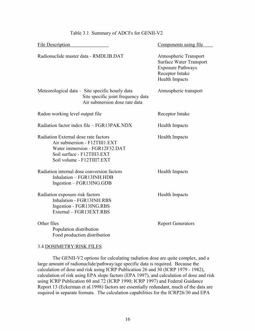
16

Table 3.1 Summary of ADCFs for GENII-V2 File Description Components using file Radionuclide master data - RMDLIB.DAT Atmospheric Transport Surface Water Transport Exposure Pathways Receptor Intake Health Impacts Meteorological data – Site specific hourly data Atmospheric transport Site specific joint frequency data Air submersion dose rate data Radon working level output file Receptor Intake Radiation factor index file – FGR13PAK.NDX Health Impacts Radiation External dose rate factors Health Impacts Air submersion - F12TIII1.EXT

Water immersion - FGR12F32.DAT Soil surface - F12TIII3.EXT Soil volume - F12TIII7.EXT

Radiation internal dose conversion factors Health Impacts Inhalation – FGR13INH.HDB Ingestion – FGR13ING.GDB Radiation exposure risk factors Health Impacts Inhalation - FGR13INH.RBS Ingestion - FGR13ING.RBS External – FGR13EXT.RBS Other files Report Generators Population distribution Food production distribution 3.4 DOSIMETRY/RISK FILES The GENII-V2 options for calculating radiation dose are quite complex, and a large amount of radionuclide/pathway/age specific data is required. Because the calculation of dose and risk using ICRP Publication 26 and 30 (ICRP 1979 - 1982), calculation of risk using EPA slope factors (EPA 1997), and calculation of dose and risk using ICRP Publication 60 and 72 (ICRP 1990; ICRP 1997) and Federal Guidance Report 13 (Eckerman et al.1998) factors are essentially redundant, much of the data are required in separate formats. The calculation capabilities for the ICRP26/30 and EPA

17

slope factor methods are derived from parallel capabilities in the MEPAS code system (Whelan et al. 1992), and so the data are available within the FRAMES system. As described in the next section, the ICRP-60 and Federal Guidance Report 13 methods are derived from methods developed for EPA at Oak Ridge National Laboratory. 3.4.1 Radiation Dose Factor Index File The dose and risk factors provided with the GENII-V2 system were developed at Oak Ridge National Laboratory for Federal Guidance Report 13 (Eckerman et al. 1998). The internal (inhalation and ingestion) age-dependent dose conversion factors are the basis of those found in ICRP Publications 60 through 72. Because the development of the files containing these factors was independent of the RMDLIB.DAT file, the file structure differs from that of the rest of the GENII-V2 files. The file FGR13PAK.NDX allows the GENII-V2 system to have direct access to the dose and risk files. This file has radionuclide identifiers, half-life information, and cross-reference line numbers for the remaining data files. 3.4.2 External Dose Rate Conversion Factor Files The data files F12TIII1.EXT, F12TIII3.EXT, and F12TIII7.EXT contain factors that relate radionuclide concentrations in air, soil surface, and soil volume, respectively, to dose rate. Each of these files is parallel in structure and size; each radionuclide line number is identified in the index file FGR13PAK.NDX described above. Each of these files provides dose conversion factors for 24 human body organs and tissues. The data file FGR12F32.DAT is a file parallel in structure to the three taken from Federal Guidance Report 12 but containing external dose rate factors for submersion in contaminated water. This data set was added to give GENII-V2 the capability of handling these types of exposure, requiring the modification of the file reading software appropriately. These files are provided with the GENII-V2 software package, and each is used by the health impacts calculational component. Data are provided for more radionuclides than are explicitly listed in RMDLIB.DAT – however, many are considered to be implicit progeny radionuclides within the RMDLIB.DAT structure. The GENII-V2 health risk component accounts for the decay energies of the implicit progeny (those with short half-lives) in the dose rate factor assigned for the explicit parent radionuclides. The content and structure of the files are described in Appendix B. 3.4.3 Internal Dose Conversion Factor Files The files FGR13ING.GDB and FGR13INH.HDB contain age dependent radiation dose factors for the pathways of ingestion and inhalation. Each of these files is parallel in structure and size; each radionuclide line number is identified in the index file FGR13PAK.NDX described above. Each of these files provides dose conversion factors for 24 human body organs and tissues. The ingestion file further provides information

18

subdivided by the potential GI-tract uptake fraction (f1) for each radionuclide. The inhalation file provides information subdivided by the ICRP lung model retention classes F, M, and S (fast, medium, and slow clearance rates). These files are provided with the GENII-V2 software package, and each is used by the health impacts calculational component. Data are provided for more radionuclides than are explicitly listed in RMDLIB.DAT – however, many are considered to be implicit progeny radionuclides within the RMDLIB.DAT structure. The GENII-V2 health risk component accounts for the decay energies of the implicit progeny in the dose rate factor assigned for the explicit parent radionuclides. The content and structure of the files are described in Appendix B. 3.4.4 Risk Conversion Factor Files The files FGR13ING.RBS and FGR13INH.RBS contain radiation risk conversion factors for the pathways of ingestion and inhalation. Each of these files is parallel in structure and size. The file FGR13EXT.RBS provides similar factors for the external pathways of air submersion, surface soil, and soil volume. Each of these files provides risk conversion factors for15 potential human cancer sites; each radionuclide line number is identified in the index file FGR13PAK.NDX described above. The ingestion file further provides information subdivided by the intake pathways of drinking water and food, as described in Federal Guidance Report 13, for each radionuclide. The inhalation file provides information subdivided by the ICRP lung model retention classes F, M, and S (fast, medium, and slow clearance rates). These files are provided with the GENII-V2 software package, and each is used by the health impacts calculational component. Data are provided for more radionuclides than are explicitly listed in RMDLIB.DAT – however, many are considered to be implicit progeny radionuclides within the RMDLIB.DAT structure. The GENII-V2 health risk component accounts for the decay energies of the implicit progeny in the dose rate factor assigned for the explicit parent radionuclides. The content and structure of the files are described in Appendix B. 3.5 RADON OUTPUT FILES If requested, the GENII V2 NESHAPS receptor intake module prepares a file of radon Working Levels and Working Level Months for each exposure location. This file has the extension *.WLM, and it may be accessed with any standard ASCII text editor. In current GENII versions (2.0x) this option is non-functional. 3.6 REFERENCES FOR SECTION 3 Eckerman, K.F. R.W. Leggett, C.B. Nelson, J.S. Puskin, and A.C.B. Richardson. Health Risks from Low-Level Environmental Exposure to Radionuclides, Federal Guidance Report No. 13, Part 1 – Interim Version. Office of Radiation and Indoor Air, United States Environmental Protection Agency, Washington, D.C.

19

EPA. 1997. Health Effects Assessment Summary Tables, EPA/540/R-97-036. U.S. Environmental Protection Agency, Washington, DC. International Commission on Radiological Protection (ICRP). 1979a. ICRP Publication 30, Part 1, Limits for Intakes of Radionuclides by Workers." Annals of the ICRP, Vol. 2, No. 3/4. Pergamon Press, New York, New York. International Commission on Radiological Protection (ICRP). 1979b. "ICRP Publication 30, Supplement to Part 1, Limits for Intakes of Radionuclides by Workers." Annals of the ICRP, Vol. 3, No. 1-4. Pergamon Press, New York, New York. International Commission on Radiological Protection (ICRP). 1980. "ICRP Publication 30, Part 2, Limits for Intakes of Radionuclides by Workers." Annals of the ICRP, Vol. 4, No. 3/4. Pergamon Press, New York, New York. International Commission on Radiological Protection (ICRP). 1981a. "ICRP Publication 30, Supplement to Part 2, Limits for Intakes of Radionuclides by Workers." Annals of the ICRP, Vol. 5, No. 1-6. Pergamon Press, New York, New York. International Commission on Radiological Protection (ICRP). 1981b. "ICRP Publication 30, Part 3 Including Addendum to Parts 1 and 2, Limits for Intakes of Radionuclides by Workers." Annals of the ICRP, Vol. 6, No. 2/3. Pergamon Press, New York, New York. International Commission on Radiological Protection (ICRP). 1982a. "ICRP Publication 30, Supplement A to Part 3, Limits for Intakes of Radionuclides by Workers." Annals of the ICRP, Vol. 7, No. 1-3. Pergamon Press, New York, New York. International Commission on Radiological Protection (ICRP). 1982b. "ICRP Publication 30, Supplement B to Part 3 Including Addendum to Supplements to Parts 1 and 2, Limits for Intakes of Radionuclides by Workers." Annals of the ICRP, Vol. 8, No. 1-3. Pergamon Press, New York, New York. International Commission on Radiological Protection (ICRP). 1990. "1990 Recommendations of the International Commission on Radiological Protection." Annals of the ICRP, Vol. 21, No. 1-3. Pergamon Press, New York, New York. International Commission on Radiological Protection (ICRP). 1996. "Age-dependent Doses to Members of the Public from Intake of Radionuclides: Part 5 – Compilation of Ingestion and Inhalation Dose Coefficients." Annals of the ICRP, Vol. 26, No. 1. Pergamon Press, New York, New York. Whelan, G. , J.W. Buck, D.L. Strenge, J.G. Droppo, Jr., and B.L. Hoopes. 1992. “Overview of the Multimedia Environmental Pollutant Assessment System (MEPAS),” Hazardous Waste and Hazardous Materials, Vol. 9, No. 2, pp. 191-208

20

4.0 SENSITIVITY USER INTERFACE The uncertainty and sensitivity analysis is controlled by the sensitivity user interface (SUI) which provides the capability to perform uncertainty and sensitivity analyses for user specific portions of the environmental analysis process. FRAMES provides SUI software interface and the calculational component Sensitivity/Uncertainty Module for Multimedia Models (SUM3). This section describes the purpose and scope of the uncertainty and sensitivity use interface, and describes the mathematical approaches and algorithms used in the stochastic analyses of SUM3. Section 4.1 describes the interface and structure. Section 4.2 provides: i) the conceptual background for interpreting the statistical algorithms and their use in generating random variables, ii) a description of the efficient Latin hypercube sampling approach to obtaining correlated or uncorrelated random vectors from univariate random variables, and iii) an identification of the univariate statistical distributions available and the algorithms used for random generation. Section 4.3 discusses the methods and algorithms used for uncertainty analysis results. References for this section are given in Section 4.4. A separate description of the application of SUM3 to the GENII-V2 modules is provided in the GENII-V2 users’ guide. 4.1 INTERFACE The sensitivity user interface allows the user to define the scope of the uncertainty and sensitivity analyses to be performed, activates the calculational component SUM3 to perform the repetitive calculations, and finally performs the sensitivity analysis of results. For each module included by the user in the specific analysis, the user is allowed to select parameters to be varied in the uncertainty/sensitivity analysis. The parameters available for this analysis are determined by the developers of the specific modules – primarily to prevent stochastic variation of control parameters. A summary of parameters available to the user for each of the GENII-V2 modules is given in Appendix E. The user is allowed to select and define probability distributions for each of the parameters for the sensitivity/uncertainty analysis. The distributions available to the user are described in the following sections. 4.2 MATHEMATICAL STRATEGIES FOR GENERATING RANDOM VARIABLES This section presents random-number-generation theory and algorithms for statistical distributions implemented in the SUM3 module of FRAMES. This module is available for all GENII-V2 modules. The topics addressed are probability concepts, including generation of uniform random numbers, the concepts of stratified and Latin Hypercube sampling (LHS) and algorithms for random-number generation. 4.2.1 Probability Concepts for Univariate Random Number Generation The distribution of a continuous random variable X (the term "continuous" indicates that the random variable is defined over a continuum of values) is completely described by its probability density function f(x) (referred to as a PDF). The interpretation of the PDF is

21

that the area under f(x) over an interval a<x<b equals the probability that the random variable, X, will fall in the interval (a,b) and is denoted by P[a<X<b]. The integral of the f(x) over the entire support (the interval [L,U]) of X equals 1 (Strait 1989, p.24). The integral of the PDF from the lower bound L to some value x (that is less than the upper bound U) represents the probability that X will be observed in the interval (L,x). This integral operation defines the cumulative distribution function (CDF) for the random variable X. The CDF is denoted by F(x) and is represented mathematically by the equation

The complementary cumulative distribution function (CCDF) is found from the simple relationship 1-F(X). It represents the probability that X will occur in the interval (x,U). The limits L and U do not necessarily have to be finite. The inverse CDF, F-1(x), is single-valued if x is in the interval (L,U). Hence if p'= F(x') is known, in theory x'= F-1(p') exists. This inverse relation is important in the generation of random numbers on a computer. In practice there are situations for which no analytic expressions for F(x) or F-1(p) are available, so approximate numerical expressions are used instead. 4.2.1.1 Random Number Generation by the Probability Integral Transform Method The probability integral transform (PIT) method for generating random variables is utilized. In the PIT method, the random variable of interest is expressed as a function of a U(0,1) random variable, where U(0,1) denotes the continuous random variable ranging uniformly over the interval (0,1). The PDF of the uniform random variable is g(u)=1 if u(0,1) and is zero elsewhere. The CDF for this random variable is G(u)=u. It can be shown that any CDF evaluated at a random value X (instead of being evaluated at a known value x) is distributed uniformly over the interval (0,1) (Mood et al. 1974, p. 202). Therefore, given a realization u of the U(0,1) random variable and a known statistical distribution, one can set u= F(x) and solve this equation to obtain x = F-1(u). The value x thus obtained is a realization from the desired statistical distribution. In principle, one can obtain an exact solution for x given any statistical distribution and value u. In reality, there are some distributions, including the normal distribution and lognormal distributions, for which no closed-form analytical expression for F or F-1 exists. In these cases, approximations to the analytical expressions are applied. The PIT method allows efficient sampling for the variable X from a subregion of the interval (L,U), such as (c,d) where L<c<d<U. The following steps are required: Find the corresponding interval in the uniform domain, say (c',d') from c'=F(c) and

d'=F(d). Sample uniformly over the interval (0,1) to get a value u.

ds f(s) = F(x) xL (4.1)

22

Form the value u' corresponding to the subregion using the transformation u'=(d'-c')u+c'.

Obtain x as usual using x = F-1(u'). If any distribution is truncated to the interval (c,d), the modified PDF on that interval is expressed by

and is set to 0 outside the interval. The divisor in the density function ensures that fT(x) integrates to unity. 4.2.1.2 Dependence on the Uniform Random Number Generator Desirable attributes of a random-number generator are ease and portability of implementation, independence between generated deviates, and long cycles between recurrence of values. Using the PIT method, the degree to which each of these features is satisfied is completely related to the quality of the uniform random-number generator selected. This relationship is guaranteed by the monotonicity of F-1. The use of a suitable uniform random-number generator is central to the successful use of the PIT method. 4.2.2 Latin Hypercube Sampling The Latin Hypercube Sampling (LHS) method is a high-dimensional extension of the Latin square experimental design, in which n random vectors of dimension p are drawn at random from p populations. The n realizations in the kth vector position represent a stratified sample from the kth marginal distribution, wherein the probability content of each of the stratified intervals is 1/n. The LHS technique was introduced as a sampling technique to reduce the variability of a monotonic function of an output statistic (Iman et al., 1982) from that achievable using simple random sampling. The LHS method is now employed in many computer codes as an efficient method for generating vectors in which the vector elements are correlated. The LHS method has a number of desirable properties such as: The desired rank correlation between variables is approximately achieved The method does not require specification of the joint distribution of the correlated

variables, which would be impractical for more than 2 or 3 correlated variables The marginal distributions of the random variables are preserved. 4.2.2.1 Stratified Sampling To obtain a stratified sample of size n for variable X having distribution F, a sequence of uniformly distributed random numbers, vi, 0vi1; i = 1,...,n are first generated. The vi are randomly selected and are not ordered according to their magnitude. Let ri be the

F(c)-F(d)

f(x) = (x)f T (4.2)

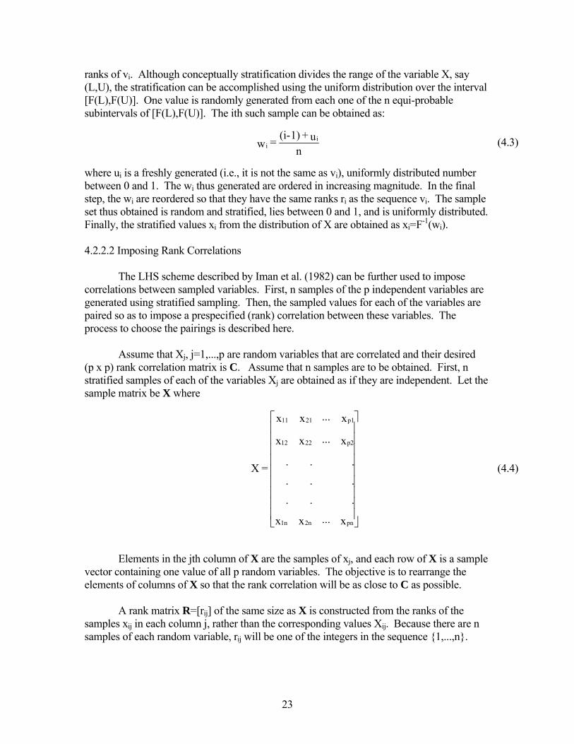
23

ranks of vi. Although conceptually stratification divides the range of the variable X, say (L,U), the stratification can be accomplished using the uniform distribution over the interval [F(L),F(U)]. One value is randomly generated from each one of the n equi-probable subintervals of [F(L),F(U)]. The ith such sample can be obtained as:

where ui is a freshly generated (i.e., it is not the same as vi), uniformly distributed number between 0 and 1. The wi thus generated are ordered in increasing magnitude. In the final step, the wi are reordered so that they have the same ranks ri as the sequence vi. The sample set thus obtained is random and stratified, lies between 0 and 1, and is uniformly distributed. Finally, the stratified values xi from the distribution of X are obtained as xi=F-1(wi). 4.2.2.2 Imposing Rank Correlations The LHS scheme described by Iman et al. (1982) can be further used to impose correlations between sampled variables. First, n samples of the p independent variables are generated using stratified sampling. Then, the sampled values for each of the variables are paired so as to impose a prespecified (rank) correlation between these variables. The process to choose the pairings is described here. Assume that Xj, j=1,...,p are random variables that are correlated and their desired (p x p) rank correlation matrix is C. Assume that n samples are to be obtained. First, n stratified samples of each of the variables Xj are obtained as if they are independent. Let the sample matrix be X where

Elements in the jth column of X are the samples of xj, and each row of X is a sample vector containing one value of all p random variables. The objective is to rearrange the elements of columns of X so that the rank correlation will be as close to C as possible. A rank matrix R=[rij] of the same size as X is constructed from the ranks of the samples xij in each column j, rather than the corresponding values Xij. Because there are n samples of each random variable, rij will be one of the integers in the sequence {1,...,n}.

nu+1)(i-

= wi

i (4.3)

x...xx

. ..

. ..

. ..

x...xx

x...xx

= X

pn2n1n

p22212

p12111

(4.4)

24

The next step is to obtain the Cholesky decomposition (Stewart, 1973, p. 142) of C as follows (because C is symmetric and nonnegative definite, such a decomposition always exists):

where P is the lower triangular matrix and PT is its transpose. Next a score matrix S is generated by using van der Waarden scores. The functional form for the scores is

where -1 is the inverse of the standard normal CDF. By construction, S has the same rank correlation matrix as X. Let U be the correlation matrix of S, whose Choleski decomposition can be written as

We want to determine a matrix T such that

Substituting for C and for U this expression leads to the expression

which yields

Although the rows of X were generated independently the sample rank correlation matrix, U, will not equal the identity matrix. The above algorithm calculates Q-1 that can be used to effectively remove the unwanted correlations. A new score matrix, S* is now determined from

which has correlation matrix C by construction.

TPP = C (4.5)

)1n+

r( = sij1-

ij (4.6)

.QQ = U T (4.7)

.TTU = C T (4.8)

TQTQ = PP TTT (4.9)

PQ = T -1 (4.10)

TS = S T* (4.11)

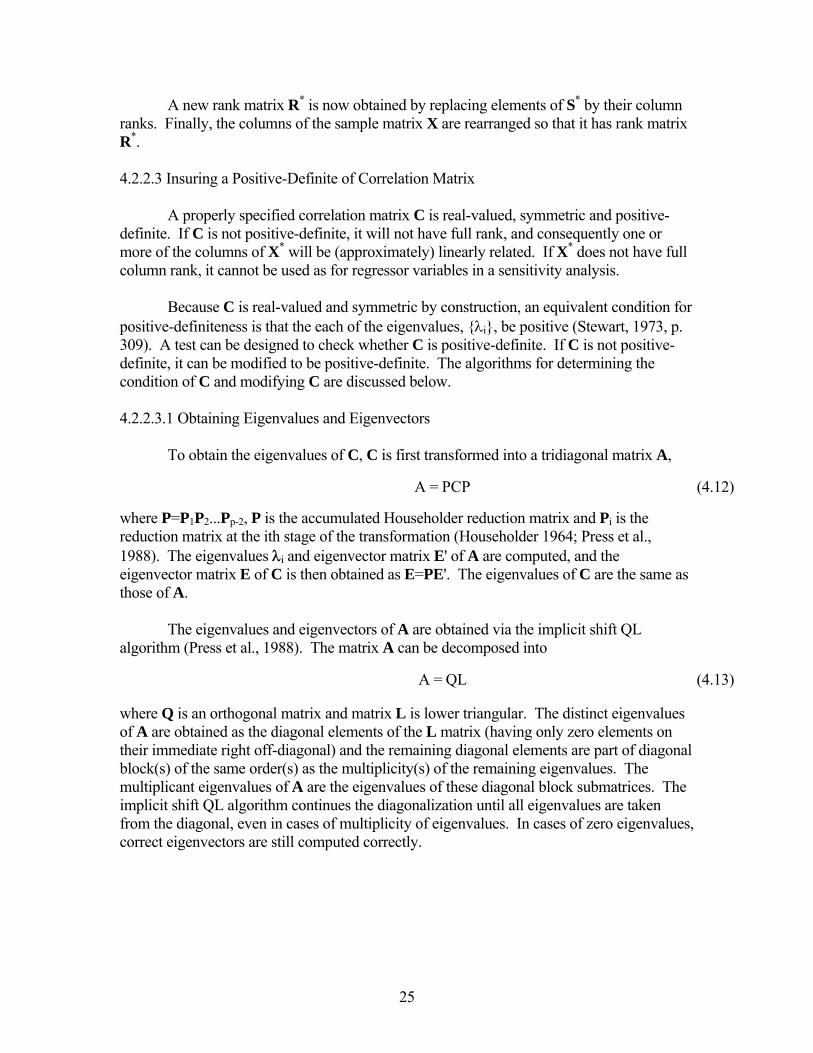
25

A new rank matrix R* is now obtained by replacing elements of S* by their column ranks. Finally, the columns of the sample matrix X are rearranged so that it has rank matrix R*. 4.2.2.3 Insuring a Positive-Definite of Correlation Matrix A properly specified correlation matrix C is real-valued, symmetric and positive-definite. If C is not positive-definite, it will not have full rank, and consequently one or more of the columns of X* will be (approximately) linearly related. If X* does not have full column rank, it cannot be used as for regressor variables in a sensitivity analysis. Because C is real-valued and symmetric by construction, an equivalent condition for positive-definiteness is that the each of the eigenvalues, {i}, be positive (Stewart, 1973, p. 309). A test can be designed to check whether C is positive-definite. If C is not positive-definite, it can be modified to be positive-definite. The algorithms for determining the condition of C and modifying C are discussed below. 4.2.2.3.1 Obtaining Eigenvalues and Eigenvectors To obtain the eigenvalues of C, C is first transformed into a tridiagonal matrix A,

where P=P1P2...Pp-2, P is the accumulated Householder reduction matrix and Pi is the reduction matrix at the ith stage of the transformation (Householder 1964; Press et al., 1988). The eigenvalues i and eigenvector matrix E' of A are computed, and the eigenvector matrix E of C is then obtained as E=PE'. The eigenvalues of C are the same as those of A. The eigenvalues and eigenvectors of A are obtained via the implicit shift QL algorithm (Press et al., 1988). The matrix A can be decomposed into

where Q is an orthogonal matrix and matrix L is lower triangular. The distinct eigenvalues of A are obtained as the diagonal elements of the L matrix (having only zero elements on their immediate right off-diagonal) and the remaining diagonal elements are part of diagonal block(s) of the same order(s) as the multiplicity(s) of the remaining eigenvalues. The multiplicant eigenvalues of A are the eigenvalues of these diagonal block submatrices. The implicit shift QL algorithm continues the diagonalization until all eigenvalues are taken from the diagonal, even in cases of multiplicity of eigenvalues. In cases of zero eigenvalues, correct eigenvectors are still computed correctly.

PCP =A (4.12)

QL =A (4.13)

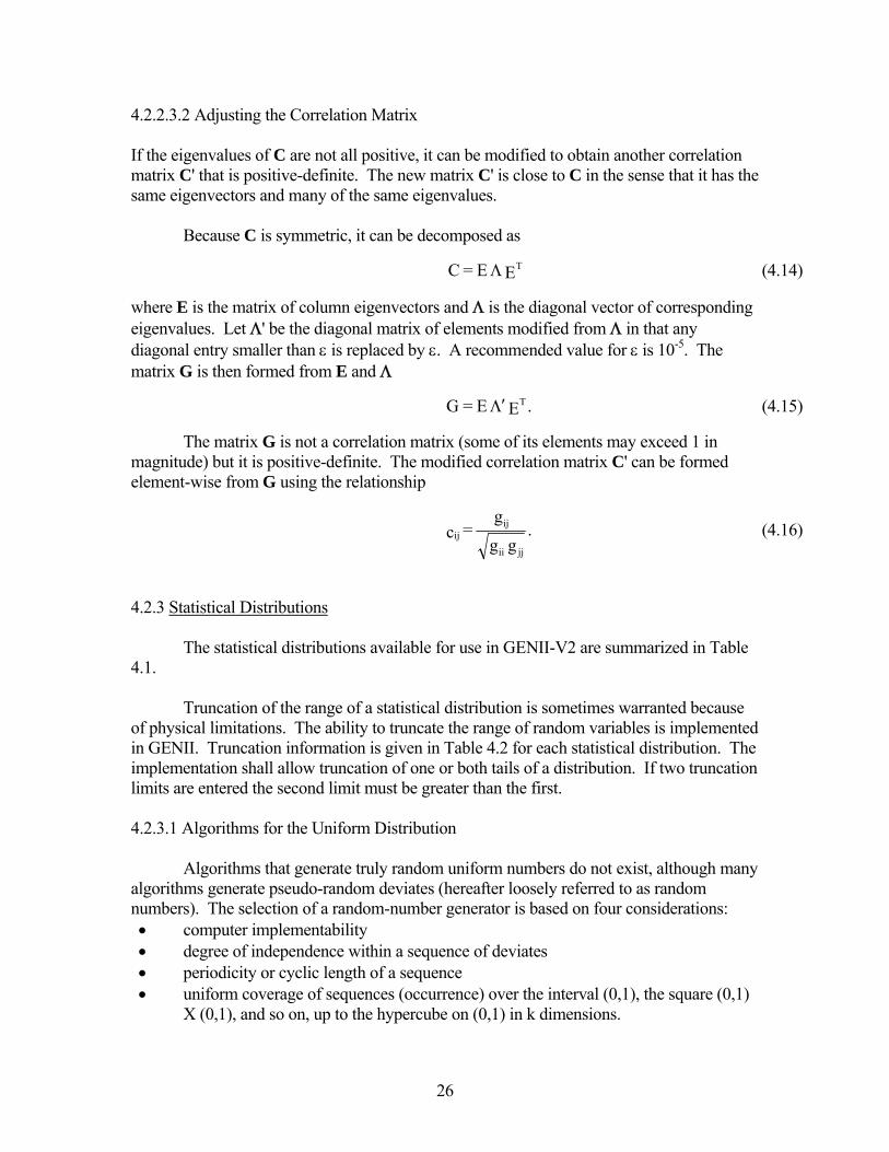
26

4.2.2.3.2 Adjusting the Correlation Matrix If the eigenvalues of C are not all positive, it can be modified to obtain another correlation matrix C' that is positive-definite. The new matrix C' is close to C in the sense that it has the same eigenvectors and many of the same eigenvalues. Because C is symmetric, it can be decomposed as

where E is the matrix of column eigenvectors and is the diagonal vector of corresponding eigenvalues. Let ' be the diagonal matrix of elements modified from in that any diagonal entry smaller than is replaced by . A recommended value for is 10-5. The matrix G is then formed from E and

The matrix G is not a correlation matrix (some of its elements may exceed 1 in magnitude) but it is positive-definite. The modified correlation matrix C' can be formed element-wise from G using the relationship

4.2.3 Statistical Distributions The statistical distributions available for use in GENII-V2 are summarized in Table 4.1. Truncation of the range of a statistical distribution is sometimes warranted because of physical limitations. The ability to truncate the range of random variables is implemented in GENII. Truncation information is given in Table 4.2 for each statistical distribution. The implementation shall allow truncation of one or both tails of a distribution. If two truncation limits are entered the second limit must be greater than the first. 4.2.3.1 Algorithms for the Uniform Distribution Algorithms that generate truly random uniform numbers do not exist, although many algorithms generate pseudo-random deviates (hereafter loosely referred to as random numbers). The selection of a random-number generator is based on four considerations: computer implementability degree of independence within a sequence of deviates periodicity or cyclic length of a sequence uniform coverage of sequences (occurrence) over the interval (0,1), the square (0,1)

X (0,1), and so on, up to the hypercube on (0,1) in k dimensions.

EE = C T (4.14)

.EE =G T (4.15)

.g g

g = c

jjii

ijij (4.16)

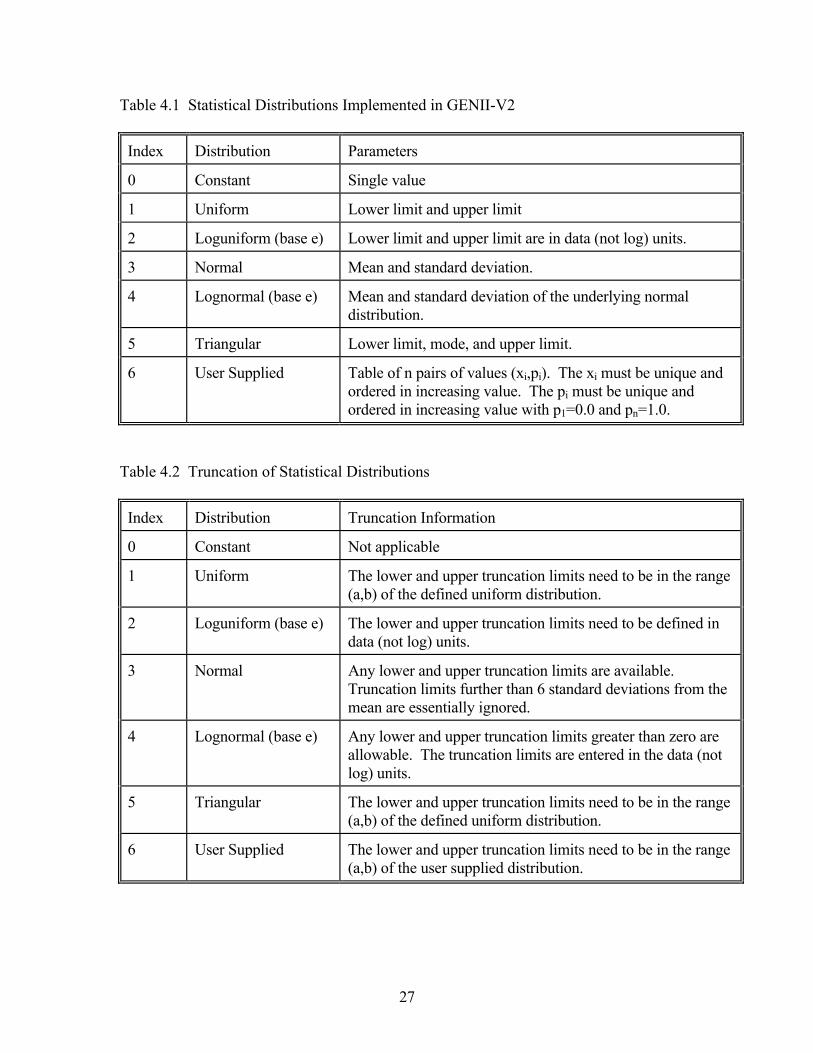
27

Table 4.1 Statistical Distributions Implemented in GENII-V2

Index Distribution Parameters

0 Constant Single value

1 Uniform Lower limit and upper limit

2 Loguniform (base e) Lower limit and upper limit are in data (not log) units.

3 Normal Mean and standard deviation.

4 Lognormal (base e) Mean and standard deviation of the underlying normal distribution.

5 Triangular Lower limit, mode, and upper limit.

6 User Supplied Table of n pairs of values (xi,pi). The xi must be unique and ordered in increasing value. The pi must be unique and ordered in increasing value with p1=0.0 and pn=1.0.

Table 4.2 Truncation of Statistical Distributions

Index Distribution Truncation Information

0 Constant Not applicable

1 Uniform The lower and upper truncation limits need to be in the range (a,b) of the defined uniform distribution.

2 Loguniform (base e) The lower and upper truncation limits need to be defined in data (not log) units.

3 Normal Any lower and upper truncation limits are available. Truncation limits further than 6 standard deviations from the mean are essentially ignored.

4 Lognormal (base e) Any lower and upper truncation limits greater than zero are allowable. The truncation limits are entered in the data (not log) units.

5 Triangular The lower and upper truncation limits need to be in the range (a,b) of the defined uniform distribution.

6 User Supplied The lower and upper truncation limits need to be in the range (a,b) of the user supplied distribution.

28

Linear congruential methods (Kennedy and Gentle 1980, pp. 136, 150) are commonly used on digital computers. The SUM3 processor called by GENII-V2 uses a linear congruential random-number generator. 4.2.3.1.1 Generation Algorithm

The uniform distribution algorithm consists of a uniform (0,1) generator and a uniform (a,b) generator. 4.2.3.1.1.1 Uniform (0,1) Generator A linear congruential generator generates random integers using an algorithm of the form

where Ri is the ith random integer to be generated between 1 and M-1, A and C are constants, M is the modules of the generated integers, and mod denotes the remainder function. These integers are converted to approximate U(0,1) numbers by the division

The period of a sequence {Ui} of generated deviates is the minimal value k such that Ui = Ui+k (this occurs independent of i for linear congruential generators). It can be shown that the period of any congruential generator does not exceed M. Therefore, if one is generating many uniform deviates, it is desirable that M be large. The performance of each congruential generator (each choice of A, C, and M) can thus be examined with respect to criteria proceeding from the four considerations given above. The SUM3/GENII-V2 implementation uses A=16807 and M=2147483647. These choices of A and M yield a sequence {Ui} that: is implementable on a 32-bit computer without machine language coding is sufficiently independent on an element-by-element basis possesses a long cycle (period) has a reasonable degree of coverage over all hypercubes of dimension less than k. These attributes proceed from results from tests described by Fishman and Moore (1986). 4.2.3.1.1.2 Uniform (a,b) Generator The uniform distribution on the interval (a,b) will be denoted by U(a,b). Any value x generated from the uniform (a,b) distribution in the GENII system makes use of a value y from the U(0,1) distribution. The value y is generated first, then x is evaluated as x = a+(b-a)y.

M mod C + R A = R 1i-i (4.17)

M / R = U ii . (4.18)

29

4.2.3.2 Algorithm for the Loguniform Distribution Loguniform distributions have a uniform distribution of the exponent. 4.2.3.2.1 Definition of the PDF The PDF for a loguniform random variable of base b is

for -<c<d<, where I is an indicator function (0 if false, 1 if true), b is the logarithm base, and ln(b) denotes the natural logarithm of b. 4.2.3.2.2 CDF and Inverse CDF Algorithms The CDF algorithm for the loguniform distribution is

The logarithm base b is chosen to be the natural constant e. The inverse CDF algorithm used to generate a value x from the loguniform distribution first generates a value y from the U(c,d) distribution and then evaluates the expression x = bu. 4.2.3.3 Algorithms for the Normal Distribution

The bell-shaped normal distribution is commonly used for many parameters. 4.2.3.3.1 Definition of the PDF A normally distributed random variable with mean and variance 2, denoted as N(,), has the PDF

for - < x < , - < < and 2 > 0. The CDF has no closed-form analytical expression.

ln(b) c)x(d-

)b<x<bI( = f(x)

dc

(4.19)

b xif

bxb if

b xif

1

ln(b)] c)[(d- / ln(b)] c - [ln(x)

0

= F(x)d

dc

d

(4.20)

e )(2

1 = f(x) 2

2

2

)(x--

(4.21)

30

4.2.3.3.2 CDF Algorithm A N(,2) random deviate, y, is obtained by generating a N(0,1) deviate, x, then transforming as y = +x. This description of the generation of normal random variables will therefore focus on the N(0,1) parameterization. The first step in the algorithm for the CDF of the standard normal distribution is to compute the area in the smallest "tail," evaluated from x to the lower or upper limit of the range of x, depending on the sign of x. Let T(x) be that area defined as T(x)=Prob[X<s] for s<0, or Prob[X>s] for s0. Thus F(x)=T(x) for x<0 and F(x)=1-T(x) for x0. The approx-imation used for T(x) is that of Adams (1969) and is given by

for |x| 1.28,

for 1.28 < x UTZERO or 1.28 < -x LTONE, and T(x)=0 for x>UTZERO or x<-LTONE. The algorithm uses z=|x| and y = z2/2. Values for the coefficients ai and bi are given in Table 4.3. A FORTRAN implementation of this algorithm is available in Hill (1985). The values UTZERO and LTONE are machine-dependent. The variable UTZERO represents the upper tail limit of the statistical density such that P[X>UTZERO] = 0 at machine accuracy, and LTONE represents the lower tail limit such that P[X>LTONE] = 1 at machine accuracy. If n denotes the decimal length of real numbers for the machine being used, and w denotes the smallest allowable positive real number, LTONE = (n+9)/3 and UTZERO = -0.3+[-2ln(w)-2]0.5. 4.2.3.3.3 Inverse CDF Algorithm The inverse CDF for the N(0,1) random variable is approximated by

where q = p-0.5, and r = (ln(0.5-|q|))0.5. The quantity (0.5-|q|) is formed as p or, to avoid cancellation if p is small, as (1-p). The letters A, B, C, and D represent polynomials of order 3, 4, 3, and 2, respectively, whose coefficients are given by Beasley and Springer (1985), and sgn(q) = 1 if q > 0 and -1 if q < 0.

)]a(y+ / )a+a[y+ / )a+a(y+ / y)a+a(z - 0.5 = T(x) 7654321 (4.22)

) ] )]b(z+ / )b+b[(z+ / )b+b(z+ / )b+b(z+

/)b+b[(z+ / )b+b((z+ / y)exp(- b = T(x)

1211109876

54321 (4.23)

0.42 |q| if

0.42 < |q| if

/D(r)C(r) sgn(q)

)q/B()qA( q = (p)F

221-

(4.24)

31

Table 4.3 Coefficients in the Normal CDF Algorithm

i ai bi

1 0.398942280444 0.398942280385

2 -0.399903438504 -3.8052E-8

3 5.75885480458 1.00000615302

4 -29.8213557808 3.98064794E-4

5 2.62433121679 1.98615381364

6 48.6959930692 -0.151679116635

7 5.92885724438 5.29330324926

8 NA 4.8385912808

9 NA -15.1508972451

10 NA 0.742380924027

11 NA 30.789933034

12 NA 3.99019417011

4.2.3.3.4 Precision The approximation for the normal CDF is accurate to 9 decimal digits on a machine with that accuracy (Hill 1985). The algorithm is implemented in double precision, so it achieves the desired accuracy on a machine with a 32-bit word length. The polynomial approximation for the inverse normal CDF is accurate up to 2-31 in the domain of p [e.g., |p'-p|< 2-31, where p' is the actual value of F(xp')]. Consideration of roundoff error brings the accuracy to the order of 20 times the least significant bit in the machine's mantissa (in the domain of p). The actual accuracy of xp is of concern, however, and is linearly approximated by

This error approximation is identical (up to a constant) for the truncated distribution.

e p)-p( )(2 = x-x )p2x(0.5

pp (4.25)

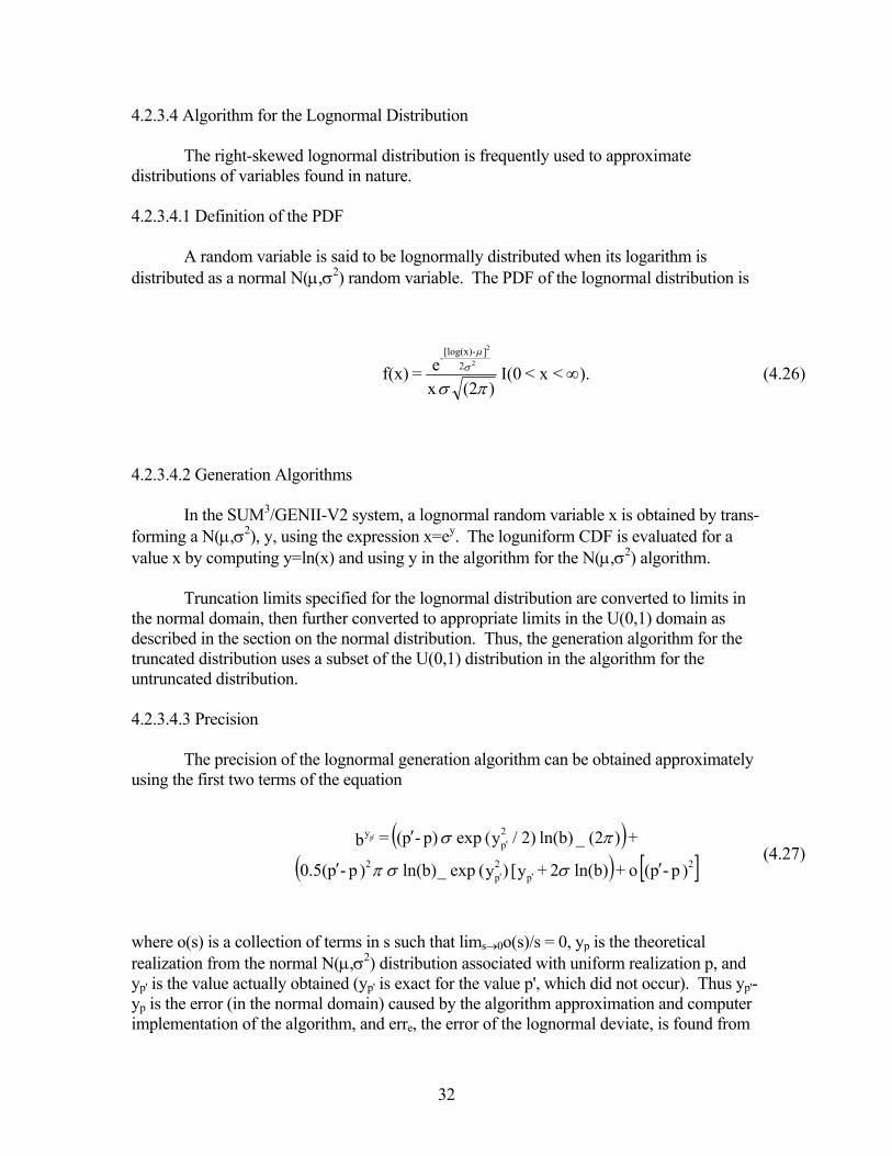
32

4.2.3.4 Algorithm for the Lognormal Distribution The right-skewed lognormal distribution is frequently used to approximate distributions of variables found in nature. 4.2.3.4.1 Definition of the PDF A random variable is said to be lognormally distributed when its logarithm is distributed as a normal N(,2) random variable. The PDF of the lognormal distribution is

4.2.3.4.2 Generation Algorithms In the SUM3/GENII-V2 system, a lognormal random variable x is obtained by trans-forming a N(,2), y, using the expression x=ey. The loguniform CDF is evaluated for a value x by computing y=ln(x) and using y in the algorithm for the N(,2) algorithm. Truncation limits specified for the lognormal distribution are converted to limits in the normal domain, then further converted to appropriate limits in the U(0,1) domain as described in the section on the normal distribution. Thus, the generation algorithm for the truncated distribution uses a subset of the U(0,1) distribution in the algorithm for the untruncated distribution. 4.2.3.4.3 Precision The precision of the lognormal generation algorithm can be obtained approximately using the first two terms of the equation

where o(s) is a collection of terms in s such that lims0o(s)/s = 0, yp is the theoretical realization from the normal N(,2) distribution associated with uniform realization p, and yp' is the value actually obtained (yp' is exact for the value p', which did not occur). Thus yp'-yp is the error (in the normal domain) caused by the algorithm approximation and computer implementation of the algorithm, and erre, the error of the lognormal deviate, is found from

).<x<I(0 )(2x

e = f(x)2

2

2]-[log(x)

-

(4.26)

)p-p( o + ln(b) 2+y[ )y( exp _ln(b) )p-p0.5(

+ )(2 _ln(b) 2) / y( exp p)-p( = b2

p2p

2

2p

yp

(4.27)

33

The bound on |p'-p| is given in the description of the normal deviate generation.

binbinbin pn,i

n

k=i

pn,i

n

k=i

pn,i

1-k

k=i 21

2

1

- = (4.29)

4.2.3.5 User-Specified Distribution In addition to selecting from the foregoing families of distributions, the user may implement any other distribution by supplying a table of data pairs corresponding to [x,F(x)]. Thus, the user can provide SUM3/GENII-V2 with discrete evaluations of the CDF. The algorithm linearly interpolates between these points to solve for F-1(u) when generating a deviate or determining truncation limits in the domain of the uniform U(0,1) distribution. 4.3 UNCERTAINTY ANALYSIS METHODS The analysis of uncertainty entails using one or more tools to present the uncertainties in output results and their statistics. This section describes the tools for uncertainty analysis that are available in the SUM3/GENII-V2 system. 4.3.1 CDF's and CCDF's The cumulative distribution function, F(x), for a random variable (Mood et al., 1974), X, is cumulative probability or probability that a realization of X will not exceed a given value, F(x) = Prob[Xx]. This function is nondecreasing and takes on values from 0 to 1. A slowly increasing CDF indicates a large variability of X, while a rapid increase in the CDF reflects a smaller degree of variability of X. If X is continuously distributed, the inflection point of the CDF occurs at the mode of the distribution. The 100pth percentile of the distribution is obtained as

If X is from a continuous distribution and 0<p<1, then

For example, the median (50th percentile) and the 90th percentile are obtained as above using p=.5 and p=.9, respectively.

.b-b = err pyye

pp (4.28)

} pF(x) : x{ minimum = p (4.30)

. (p)F = -1p (4.31)

34

Because the true cumulative distribution function is generally not known, the empirical cumulative distribution function is used as an estimate of the CDF. Given the observed data x1,...,xn, the empirical distribution function is computed as:

.x)x(n

1 = (x)F i

n

1=in (4.32)

where (A) is 1 or 0 according as A is true or false. Although the empirical CDF, being a sum of step functions, is discontinuous for small sample sizes, as n gets large, this function becomes increasingly continuous and smooth if X is from a continuous probability distribution. If one is interested in exceedence probabilities rather than cumulative probabilities, the CCDF, G n, can be more useful than the CDF. Gn(x) is obtained as Gn(x) = 1-Fn(x). 4.3.2 Sample Mean, Quantiles and their Corresponding Confidence Limits 4.3.2.1 Sample Mean and Confidence Limits The sample mean, defined as

is commonly used as an estimate for the population mean, µ (=E[X]). Because the sample mean is also random, the degree of its uncertainty is frequently expressed as a 100(1-2) percent (random) confidence interval [l,u] such that the statement Prob[lµu] = 1-2. (The term is called a “percentage point.”) The confidence interval computed in the GENII system is the interval is based upon the normal-theory approximation,

where

and t 1n- is the upper 100(1-)th quantile of the Student t distribution having n-1 degrees of

freedom. Letting m=n-1, if n-1100 the upper 100(1-)th quantile of the normal distribution, z, is used in lieu of the t distribution. This normal quantile is computed as in Section 2.3.3.2. If n-1<100 the quantile from the t distribution is used, being obtained as (Kennedy et al., 1980)

xn

1 = x i

n

1=in (4.33)

st n

1_+ x n1n-n

(4.34)

)x-x(1n-

1=s

2ni

n

1=in (4.35)

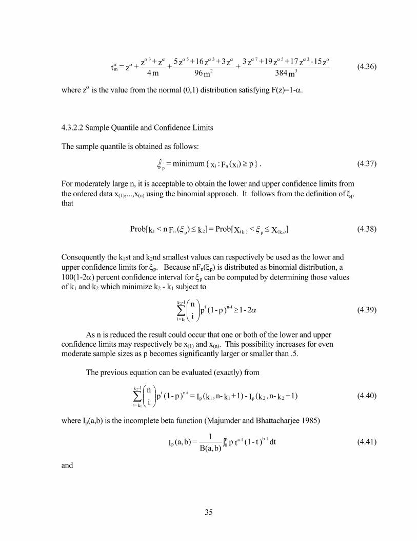
35

where z is the value from the normal (0,1) distribution satisfying F(z)=1-. 4.3.2.2 Sample Quantile and Confidence Limits The sample quantile is obtained as follows:

For moderately large n, it is acceptable to obtain the lower and upper confidence limits from the ordered data x(1),...,x(n) using the binomial approach. It follows from the definition of p that

Consequently the k1st and k2nd smallest values can respectively be used as the lower and upper confidence limits for p. Because nFn(p) is distributed as binomial distribution, a 100(1-2) percent confidence interval for p can be computed by determining those values of k1 and k2 which minimize k2 - k1 subject to

As n is reduced the result could occur that one or both of the lower and upper confidence limits may respectively be x(1) and x(n). This possibility increases for even moderate sample sizes as p becomes significantly larger or smaller than .5. The previous equation can be evaluated (exactly) from

where Ip(a,b) is the incomplete beta function (Majumder and Bhattacharjee 1985)

and

m384

z15-z17+z19+z3 +

m96z3+z16+z5

+m4

z+z+z = t 3

3 5 7

2

3 5 3

m

(4.36)

. } p)x(F :x { minimum = ˆinip (4.37)

]X<XProb[ = ]k)(Fn<kProb[ )k(p)k(2pn1 21 (4.38)

2-1 )p-(1 p i

n in-i1-k

k=i

2

1

(4.39)

1)+kn-,k(I - 1)+kn-,k(I = )p-(1 p i

n22p11p

in-i1-k

k=i

2

1

(4.40)

dt )t-(1 t p b)B(a,

1 = b)(a,I

1b-1a-p0p (4.41)

36

For integer a (which applies here), (a)=(a-1)!. An approximation for Ip(a,b) is available (Press et al., 1988). Let w = (np(1-p))0.5 and let z/2 be the 100(1-/2) upper percentile of the Normal(0,1) distribution. Initial values for k1 and k2 are found from:

These initial values of k1 and k2 are accurate to within 1 or 2 for all n greater than 20. 4.4 REFERENCES FOR SECTION 4 Adams, A.G. 1969. “Area Under the Normal Curve,” Algorithm 39, Computer Journal, Vol. 12, pp. 197-198. Beasley, J.D., and S.G. Springer. 1985. “The Percentage Points of the Normal Distribution,” Algorithm AS 111 in Applied Statistics Algorithms, P. Griffiths and I.D. Hill, Eds., Ellis Horwood Limited, Chichester, United Kingdom. Fishman, G. S., and L. R. Moore. 1986. "An Exhaustive Analysis of Multiplicative Congruential Random Number Generators with Modulus 231-1." SIAM Journal of Scientific and Statistical Computing 7(1):24-44. Hill, I. D. 1985. "The Normal Integral." Algorithm AS 66 in Applied Statistics Algorithms, eds. P. Griffiths and I. D. Hill. Ellis Horwood Limited, Chichester, United Kingdom. Householder, A.S. 1964. The Theory of Matrices in Numerical Analysis. Boston, Ginn (Blaisdell). Iman, R.L. and Conover, W.J. 1982. "A Distribution-Free Approach to Inducing Rank Correlation Among Input Variables," Communications in Statistics: Simulation and Computation, B11(3):311-334. Kennedy, W.J., Jr., and Gentle, J.E. 1980. Statistical Computing. New York, Marcel Dekker. Majumder, K. L., and G. P. Bhattacharjee. 1985. "The Incomplete Beta Integral." Algorithm AS 63 in Applied Statistics Algorithms, eds. P. Griffiths and I. D. Hill. Ellis Horwood Limited, Chichester, United Kingdom.

(b)(a)

b)(a+=b)B(a,

(4.42)

0.5 + z w+ np = k

0.5 + z w- np = k

2/2

2/1

(4.43)

37

Mood, A. M, F. A. Graybill, and D. C. Boes. 1974. Introduction to the Theory of Statistics, 3rd ed. McGraw-Hill, New York. Press, W.H., Flannery, B.P., Teukolsky, S.A., and Fetterling, W.T. 1988. Numerical Recipes in C: The Art of Scientific Computing. New York, Cambridge Univ. Press. Stewart, G.W. 1973. Introduction to Matrix Computations. New York, Academic Press. Strait, P. T. 1989. A First Course in Probability and Statistics With Applications, 2nd ed. Harcourt Brace Jovanovich, New York.

38

5.0 ATMOSPHERIC TRANSPORT AND DEPOSITION MODULES

The atmospheric models, ACUTESRC, PERCENTILE, CHRONSRC, PUFCHRON, and PUFACUTE, for the GENII-V2 system, are a suite of codes to account for the transport, diffusion, deposition, depletion, and decay of radionuclides while in the atmosphere. The basic diffusion model used in this suite of codes is the Gaussian solution to the diffusion equation. Both straight-line Gaussian-plume (ACUTESRC, PERCENTILE, and CHRONSRC) and Lagrangian-puff (PUFCHRON and PUFACUTE) models are incorporated in the suite of codes. The models include estimations for both chronic (CHRONSRC and PUFCHRON) and accidental or acute (ACUTESRC, PERCENTILE, and PUFACUTE) releases. Elements of the models representing the physical processes of diffusion, deposition, depletion, cloud shine, and decay of radionuclides have been selected to be as realistic as possible yet be consistent with readily available meteorological and climatological data. In the case of dispersion coefficients and the effects of building wakes, alternative models for these physical processes have been included in the suite to provide users with flexibility.

In the rest of this section includes the descriptions of both the straight-line plume

and puff models and its components. Section 5.1 describes the straight-line plume, while Section 5.2 describes the puff models. The components of the models are described in Section 5.3. The optional air submersion dose calculations performed by these models are described in Section 5.4.

5.1 STRAIGHT-LINE GAUSSIAN PLUME MODEL

This section describes the straight-line Gaussian model. It covers the basic plume and its variations. It also describes modification of the model to account for area sources, multiple sources, and the finite flow from short stacks and vents. 5.1.1 Basic Model

The complete straight-line Gaussian plume model is

where χ = the concentration at distance x, crosswind position y, and height z, in a

plume with axis at height heff (Ci/m3) Q'(x) = the release rate, corrected for deposition and decay as appropriate (Ci/s) U(hs) = the wind speed at release height, hs (m/s) σy = the horizontal dispersion coefficient (m) σz = the vertical dispersion coefficient (m) G(z) = the vertical dispersion factor.

G(z))2

yexp(-

)hU(2

1=

(x)Q

)hH,z,y,(x,2y

2

zys

eff

(5.1)

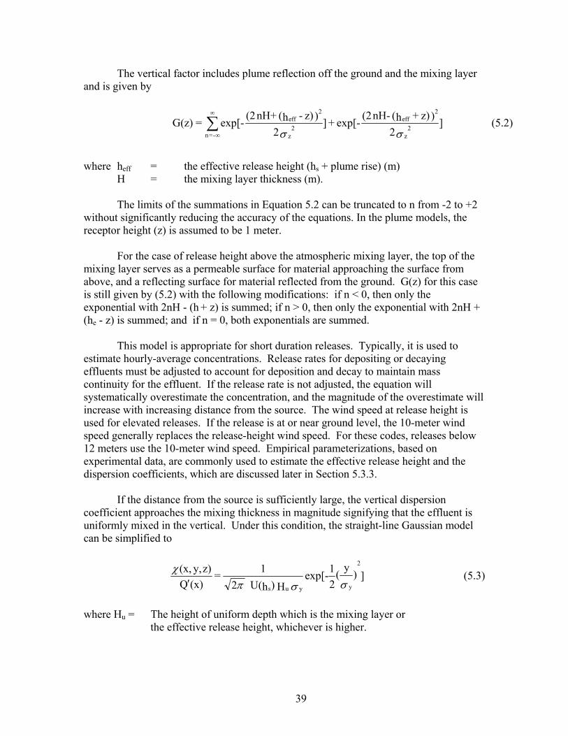
39

The vertical factor includes plume reflection off the ground and the mixing layer and is given by

where heff = the effective release height (hs + plume rise) (m) H = the mixing layer thickness (m).

The limits of the summations in Equation 5.2 can be truncated to n from -2 to +2 without significantly reducing the accuracy of the equations. In the plume models, the receptor height (z) is assumed to be 1 meter.

For the case of release height above the atmospheric mixing layer, the top of the mixing layer serves as a permeable surface for material approaching the surface from above, and a reflecting surface for material reflected from the ground. G(z) for this case is still given by (5.2) with the following modifications: if n < 0, then only the exponential with 2nH - (h + z) is summed; if n > 0, then only the exponential with 2nH + (he - z) is summed; and if n = 0, both exponentials are summed.

This model is appropriate for short duration releases. Typically, it is used to estimate hourly-average concentrations. Release rates for depositing or decaying effluents must be adjusted to account for deposition and decay to maintain mass continuity for the effluent. If the release rate is not adjusted, the equation will systematically overestimate the concentration, and the magnitude of the overestimate will increase with increasing distance from the source. The wind speed at release height is used for elevated releases. If the release is at or near ground level, the 10-meter wind speed generally replaces the release-height wind speed. For these codes, releases below 12 meters use the 10-meter wind speed. Empirical parameterizations, based on experimental data, are commonly used to estimate the effective release height and the dispersion coefficients, which are discussed later in Section 5.3.3.

If the distance from the source is sufficiently large, the vertical dispersion coefficient approaches the mixing thickness in magnitude signifying that the effluent is uniformly mixed in the vertical. Under this condition, the straight-line Gaussian model can be simplified to

])y

(2

1exp[-

H )h U(2

1 =

(x)Q

z)y,(x,

y

2

yus

(5.3)

where Hu = The height of uniform depth which is the mixing layer or

the effective release height, whichever is higher.

]2

)z)+h(nH-(2exp[-+]

2

)z)-h(nH+(2exp[-=G(z)

z2

2eff

z2

2eff

-=n

(5.2)

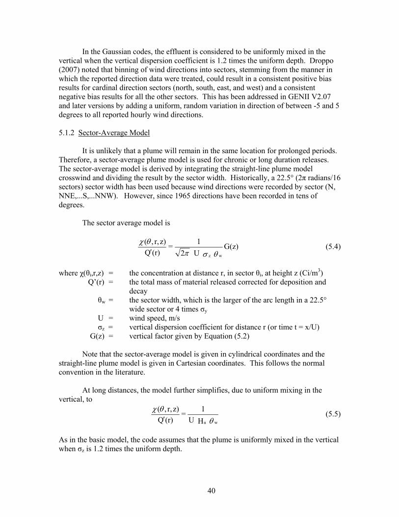
40

In the Gaussian codes, the effluent is considered to be uniformly mixed in the vertical when the vertical dispersion coefficient is 1.2 times the uniform depth. Droppo (2007) noted that binning of wind directions into sectors, stemming from the manner in which the reported direction data were treated, could result in a consistent positive bias results for cardinal direction sectors (north, south, east, and west) and a consistent negative bias results for all the other sectors. This has been addressed in GENII V2.07 and later versions by adding a uniform, random variation in direction of between -5 and 5 degrees to all reported hourly wind directions.

5.1.2 Sector-Average Model

It is unlikely that a plume will remain in the same location for prolonged periods. Therefore, a sector-average plume model is used for chronic or long duration releases. The sector-average model is derived by integrating the straight-line plume model crosswind and dividing the result by the sector width. Historically, a 22.5° (2π radians/16 sectors) sector width has been used because wind directions were recorded by sector (N, NNE,...S,...NNW). However, since 1965 directions have been recorded in tens of degrees.

The sector average model is

G(z) U2

1=

(r)Q

z)r,,(

wz

(5.4)

where χ(θi,r,z) = the concentration at distance r, in sector θi, at height z (Ci/m3) Q’(r) = the total mass of material released corrected for deposition and

decay θw = the sector width, which is the larger of the arc length in a 22.5°

wide sector or 4 times σy U = wind speed, m/s

σz = vertical dispersion coefficient for distance r (or time t = x/U) G(z) = vertical factor given by Equation (5.2)

Note that the sector-average model is given in cylindrical coordinates and the straight-line plume model is given in Cartesian coordinates. This follows the normal convention in the literature.

At long distances, the model further simplifies, due to uniform mixing in the vertical, to

wu H U

1=

(r)Q

z)r,,(

(5.5)

As in the basic model, the code assumes that the plume is uniformly mixed in the vertical when σz is 1.2 times the uniform depth.

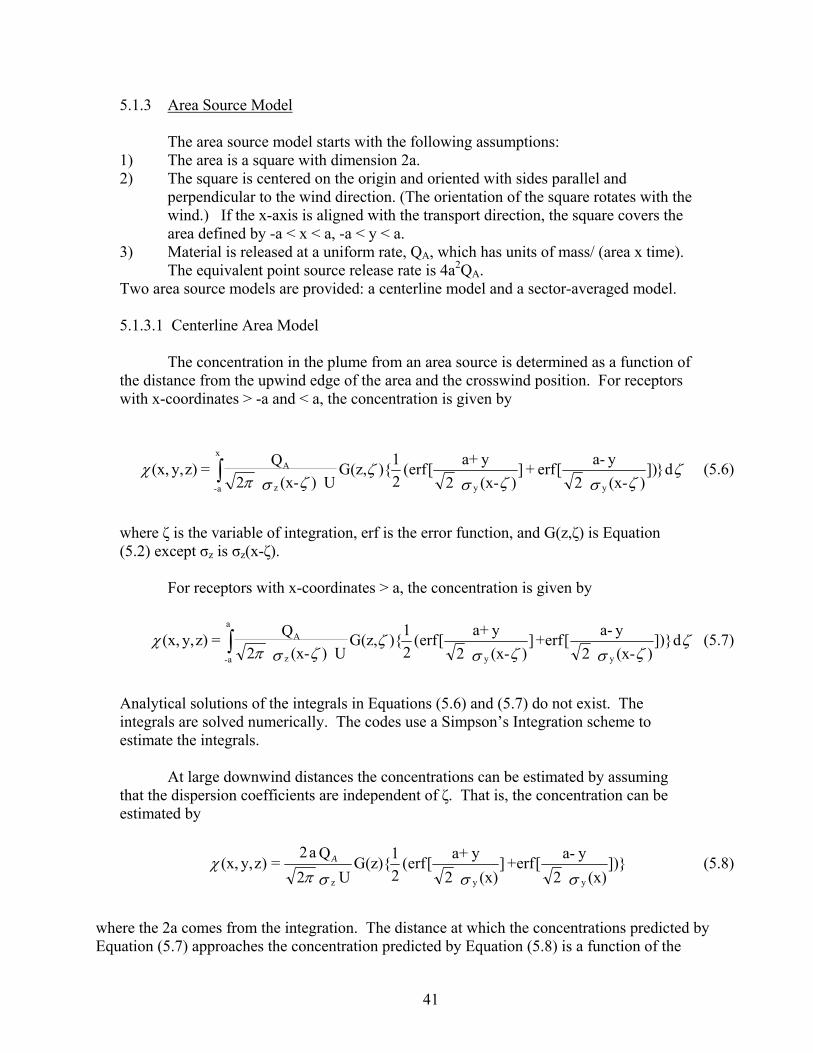
41

5.1.3 Area Source Model

The area source model starts with the following assumptions: 1) The area is a square with dimension 2a. 2) The square is centered on the origin and oriented with sides parallel and

perpendicular to the wind direction. (The orientation of the square rotates with the wind.) If the x-axis is aligned with the transport direction, the square covers the area defined by -a < x < a, -a < y < a.

3) Material is released at a uniform rate, QA, which has units of mass/ (area x time). The equivalent point source release rate is 4a2QA.

Two area source models are provided: a centerline model and a sector-averaged model. 5.1.3.1 Centerline Area Model

The concentration in the plume from an area source is determined as a function of the distance from the upwind edge of the area and the crosswind position. For receptors with x-coordinates > -a and < a, the concentration is given by

where ζ is the variable of integration, erf is the error function, and G(z,ζ) is Equation (5.2) except σz is σz(x-ζ).

For receptors with x-coordinates > a, the concentration is given by

Analytical solutions of the integrals in Equations (5.6) and (5.7) do not exist. The integrals are solved numerically. The codes use a Simpson’s Integration scheme to estimate the integrals.

At large downwind distances the concentrations can be estimated by assuming that the dispersion coefficients are independent of ζ. That is, the concentration can be estimated by

where the 2a comes from the integration. The distance at which the concentrations predicted by Equation (5.7) approaches the concentration predicted by Equation (5.8) is a function of the

d}]))(x- 2

ya-[erf + ]

)(x- 2

ya+[erf(

2

1){G(z,

U)(x- 2

Q=z)y,(x,

yyz

Ax

a- (5.6)

d])})(x- 2

ya-[erf+]

)(x- 2

ya+[erf(

2

1){G(z,

U)(x- 2

Q=z)y,(x,

yyz

Aa

a- (5.7)

])}(x) 2

ya-[erf+]

(x) 2

ya+[erf(

2

1G(z){

U 2

Qa2=)zy,(x,

yyz A (5.8)

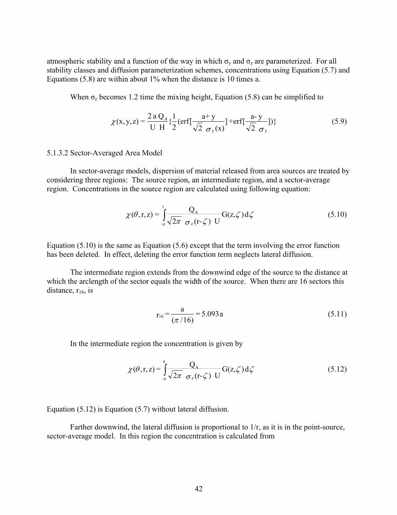
42

atmospheric stability and a function of the way in which σy and σz are parameterized. For all stability classes and diffusion parameterization schemes, concentrations using Equation (5.7) and Equations (5.8) are within about 1% when the distance is 10 times a.

When σz becomes 1.2 time the mixing height, Equation (5.8) can be simplified to

5.1.3.2 Sector-Averaged Area Model

In sector-average models, dispersion of material released from area sources are treated by considering three regions: The source region, an intermediate region, and a sector-average region. Concentrations in the source region are calculated using following equation:

Equation (5.10) is the same as Equation (5.6) except that the term involving the error function has been deleted. In effect, deleting the error function term neglects lateral diffusion.

The intermediate region extends from the downwind edge of the source to the distance at which the arclength of the sector equals the width of the source. When there are 16 sectors this distance, r16, is

In the intermediate region the concentration is given by

Equation (5.12) is Equation (5.7) without lateral diffusion.

Farther downwind, the lateral diffusion is proportional to 1/r, as it is in the point-source, sector-average model. In this region the concentration is calculated from

])} 2

ya-[erf+]

(x) 2

ya+[erf(

2

1{

H U

Q a 2=z)y,(x,

yy A (5.9)

d)G(z, U)(r- 2

Q=z)r,,(

z

Ar

a- (5.10)

a5.093 = 16)/(

a = r16

(5.11)

d)G(z, U)(r- 2

Q = z)r,,(

z

Aa

a- (5.12)

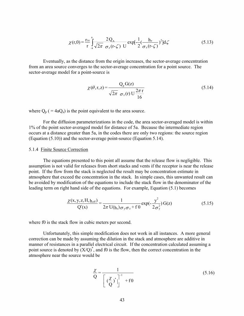
43

Eventually, as the distance from the origin increases, the sector-average concentration

from an area source converges to the sector-average concentration for a point source. The sector-average model for a point-source is

where Qp ( = 4aQa) is the point equivalent to the area source.

For the diffusion parameterizations in the code, the area sector-averaged model is within 1% of the point sector-averaged model for distance of 5a. Because the intermediate region occurs at a distance greater than 5a, in the codes there are only two regions: the source region (Equation (5.10)) and the sector-average point-source (Equation 5.14). 5.1.4 Finite Source Correction

The equations presented to this point all assume that the release flow is negligible. This assumption is not valid for releases from short stacks and vents if the receptor is near the release point. If the flow from the stack is neglected the result may be concentration estimate in atmosphere that exceed the concentration in the stack. In simple cases, this unwanted result can be avoided by modification of the equations to include the stack flow in the denominator of the leading term on right hand side of the equations. For example, Equation (5.1) becomes

where f0 is the stack flow in cubic meters per second.

Unfortunately, this simple modification does not work in all instances. A more general correction can be made by assuming the dilution in the stack and atmosphere are additive in manner of resistances in a parallel electrical circuit. If the concentration calculated assuming a point source is denoted by (X/Q)*, and f0 is the flow, then the correct concentration in the atmosphere near the source would be

d]))(r-

h(2

1[-exp

U)(r- 2

Q2

rr = (r,0) 2

z

e

z

Aa

a-

16 (5.13)

16r2

U(r) 2

G(z)Q = z)r,,(

z

p

(5.14)

G(z) )2

yexp(-

0f + )hU(2

1 =

(x)Q

)hH,z,y,(x,2y

2

zys

eff

(5.15)

0f + )Q

(

1 =

Q 1

*

(5.16)

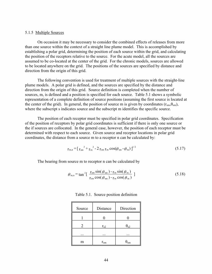
44

5.1.5 Multiple Sources

On occasion it may be necessary to consider the combined effects of releases from more than one source within the context of a straight line plume model. This is accomplished by establishing a polar grid, determining the position of each source within the grid, and calculating the position of the receptors relative to the source. For the acute model, all the sources are assumed to be co-located at the center of the grid. For the chronic models, sources are allowed to be located anywhere on the grid. The positions of the sources are specified by distance and direction from the origin of this grid.

The following convention is used for treatment of multiple sources with the straight-line plume models. A polar grid is defined, and the sources are specified by the distance and direction from the origin of this grid. Source definition is completed when the number of sources, m, is defined and a position is specified for each source. Table 5.1 shows a symbolic representation of a complete definition of source positions (assuming the first source is located at the center of the grid). In general, the position of source m is given by coordinates (rsm,θsm), where the subscript s indicates source and the subscript m identifies the specific source.

The position of each receptor must be specified in polar grid coordinates. Specification of the position of receptors by polar grid coordinates is sufficient if there is only one source or the if sources are collocated. In the general case, however, the position of each receptor must be determined with respect to each source. Given source and receptor locations in polar grid coordinates, the distance from a source m to a receptor n can be calculated by:

The bearing from source m to receptor n can be calculated by

Table 5.1. Source position definition

Source Distance Direction

1 0 0

2 rs2 θs2

... ... ...

m rsm θsm

] ) - cos( r r 2 - r + r [ = r2/1

rnsmrnsmrn2

sm2

nm, (5.17)

] ) cos( r - ) cos( r

) sin( r - ) sin( r [tan = rnrnsmsm

rnrnsmsm1-nm,

(5.18)

45

Upon completion of calculation of the positions of all receptors with respect to all sources, a matrix similar to that shown in Table 5.2 will have been filled. This matrix provides the information necessary to compute the total concentrations at each receptor. However, the information is not organized in a manner that promotes computational efficiency. To promote computational efficiency, the information in Table 5.2 will be sorted and reorganized. When the reorganization is complete the revised source/receptor position matrix will have the appearance of Table 5.3.

Given the wind direction, the relationships shown in Table 5.3 can be used to quickly

identify all receptors downwind of each source. Each receptor will appear just once for each source. However, the revised source/receptor matrix may be larger than the initial matrix because for a given wind direction there may not be an equal number of receptors downwind of all sources. For example, for the first downwind direction Table 5.3 shows two receptors downwind of source 1 and three receptors downwind of source m.

Table 5.2. Initial Source/Receptor Position Matrix

Source 1 ... Source m

Receptor

Distance Direction ... Distance

Direction

1

r1,1 θ1,1 ... rm,1

θm,1

2

r1,2 θ1,2 ... rm,2

θm,2

3

r1,3 θ1,3 ... rm,3

θm,3

...

... ... ... ...

...

n

r1,n θ1,n ... rm,n

θm,n

Table 5.3. Revised Source/Receptor Position Matrix

Downwind Direction

Source 1 ... Source m

Distance Receptor ... Distance

Receptor

θ1

r1,1 1 ... rm,n

n

θ1

r1,2 2 ... rm,3

3

θ1

r1,3 3 rm,4

4

...

... ... ... ...

...

θi

r1,n n ... rm,9

9

...

... ... ... ...

...

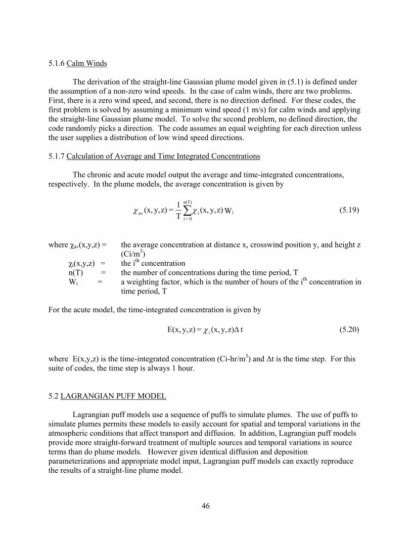
46

5.1.6 Calm Winds

The derivation of the straight-line Gaussian plume model given in (5.1) is defined under the assumption of a non-zero wind speeds. In the case of calm winds, there are two problems. First, there is a zero wind speed, and second, there is no direction defined. For these codes, the first problem is solved by assuming a minimum wind speed (1 m/s) for calm winds and applying the straight-line Gaussian plume model. To solve the second problem, no defined direction, the code randomly picks a direction. The code assumes an equal weighting for each direction unless the user supplies a distribution of low wind speed directions. 5.1.7 Calculation of Average and Time Integrated Concentrations

The chronic and acute model output the average and time-integrated concentrations, respectively. In the plume models, the average concentration is given by

where χav(x,y,z) = the average concentration at distance x, crosswind position y, and height z

(Ci/m3) χi(x,y,z) = the ith concentration n(T) = the number of concentrations during the time period, T Wi = a weighting factor, which is the number of hours of the ith concentration in

time period, T For the acute model, the time-integrated concentration is given by

where E(x,y,z) is the time-integrated concentration (Ci-hr/m3) and Δt is the time step. For this suite of codes, the time step is always 1 hour. 5.2 LAGRANGIAN PUFF MODEL

Lagrangian puff models use a sequence of puffs to simulate plumes. The use of puffs to simulate plumes permits these models to easily account for spatial and temporal variations in the atmospheric conditions that affect transport and diffusion. In addition, Lagrangian puff models provide more straight-forward treatment of multiple sources and temporal variations in source terms than do plume models. However given identical diffusion and deposition parameterizations and appropriate model input, Lagrangian puff models can exactly reproduce the results of a straight-line plume model.

Wz)y,(x, T

1=z)y,(x, ii

n(T)

0 = iav (5.19)

tz)y,(x, = z)y,E(x, i (5.20)

47

Lagrangian puff models consist of two parts, a wind field model and a diffusion model. The wind field model is used to move puffs. The diffusion model describes the spread of the puffs. This section describes the major components of Lagrangian puff models, the wind field model and the diffusion model. 5.2.1 Transport

Puff movement is determined by the wind at the center of the puff, independent of the size of the puff. The wind field model implicit in the straight-line plume model assumes that the wind direction and speed do not change in time or space. Once released to the atmosphere, material moves in a straight line with a direction defined by the wind direction at the time of release. Straight-line plume models also implicitly assume that the transport speed is immaterial. Wind fields in puff models permit curved plume trajectories and explicitly consider the transport time.

The wind model used in these codes is based upon a single meteorological station. For hourly meteorological data, this provides temporal changes in the wind speed. The model assumes spatially uniform winds, except the user can supply an array of surface roughness for each grid point on the receptor grid. This would allow the wind speed to vary spatially, but the wind direction would still be spatially uniform. See Section 5.3.2 for information on how the surface roughness effects the wind speed.

The position of a puff is determined by a series of movements starting at the time the puff is released. Hourly wind fields, based on the observed wind, are used to compute the puff movement. The number of time steps used in computing the puff movement is equal to the number of puffs released per hour (NPH) and is set as an input parameter in the codes. The time step used in puff movement is then 1/NPH and is referred to as the puff advection period. An even shorter interval, called the sampling period, is used in computing the time-integrated concentrations and surface depositions.

The puff movement is computed in a five-step process. In sequence, the steps in the process are: 1. Estimate the wind at puff transport height at the current position 2. Make an initial estimate of puff position at the end of the advection period using the

transport-height wind for the current puff position 3. Estimate the transport-height wind at this initial estimate of the puff’s position at the end

of the advection period 4. Using the winds estimated in Step 3 and the puff’s current position, make a second

estimate of the puff’s position a the end of the advection period 5. Average the position estimated in steps 2 and 4

48

The average position will be the position of the puff at the end of the advection period. These steps are described mathematically below.

The puff movement calculation begins by calculating the wind at the puff’s current

position. The wind components are based on the station’s observed friction velocity, wind direction, and surface roughness at the puff’s current position. The surface roughness of the current position is the surface roughness of the closest point on the receptor grid.

The diabatic wind profile is used to adjust the wind speed at the puff-transport height from the friction velocity and surface roughness (see Section 5.3.2). In general, the transport height of the puffs will be their effective release height. The distance moved will be calculated using the wind speed for the effective release height of the puff when the effective release height is > 10 meters and < 100 meters. The 10-meter wind speed will be used in computing movements for puff with release heights < 12 meters, and the wind speed at 100 meters will be used to compute movements of puffs with effective release heights > 100 meters. Extrapolation of wind speeds from a height of 10 meters to heights in excess of 100 meters is not considered appropriate.

Next, an initial estimate of movement is made using the components of the transport vector at the puff’s starting position. For a puff initially at x, y, z, the change in position is given by

tz)y, v(x,=y

tz)y,u(x, =x

(5.21)

where u and v are the east-west and north-south components of the wind vector, respectively, and Δt is the advection period (3600 sec/NPH). The initial estimate of the puff’s position at the end of the advection period is

y +y = y

x + x = x

(5.22)

The transport winds at this location at the current time are then determined following the

same procedure used to obtain the initial transport wind estimates.

The second set of estimates of the transport wind components is used to obtain a second estimate of the puff movement

tz),y,x v(= y

tz),y,xu( = x

(5.23)

49

Finally, the puff’s position at the end of the advection period x'', y'' is determined from the current position and the average of the two movement estimates

)y +y 0.5( +y = y

)x +x 0.5( + x = x

(5.24)

Material in a puff continues to contribute to the time-integrated air concentration and surface deposition at grid nodes near the edge of the receptor grid even after the center of the puff leaves the interior of the receptor grid as long as the puff center stays within the tracking region. The tracking region is an area surrounding the receptor grid that, along with allowing the puffs to continue to contribute air concentration and deposition to the grid, also allows the puffs to return from the tracking region to the receptor grid. Once the center of the puff moves beyond the tracking region, the puff is consider to no longer be contributing to the grid and is turned off. The size of the tracking region is a fraction of the distance from the center of the receptor grid to the various boundaries (north, south, east, and west). The fraction is normally set to 0.4, but can be altered by the user. For puffs in the tracking region, the puff movement is determined by the winds at the closest grid points on the receptor grid. 5.2.2 Puff Diffusion

In Lagrangian puff models, calculation of concentrations take place in two steps. The first step is calculation of the concentration in the puff as a function of distance from the center of the puff. The second step is calculation of concentration at a fixed point in the model domain.

The concentration in puffs is given by

where χp(r,z,t) = the concentration at a distance r from the center of the puff and height z

above ground at time t (Ci/m3) Qp(to,t) = the mass in the puff (Qp = Q'(to)Δt) released at time to corrected for

depletion and decay between to and t (Ci) σr = the radial dispersion coefficient (generally assumed to be equal to σy) (m) G(z) = The vertical factor (see Equation (5.2))

The mass in each puff is set at the time the puff is released. It is the product of the

release rate and the time separation between puffs. As each puff moves through the model domain, the mass in the puff may be adjusted to account for deposition and radioactive decay.

G(z))2rexp(-

)(2

t),t(Q = t)z,(r,

2r

2

z2r

2/3

opp

(5.25)

50

5.2.3 Calculation of Concentrations and Exposure

Calculation of the concentration at a point involves the summation of the contributions from all puffs. This summation is represented as

where χij(z,t) = the concentration at position i,j at height z at time t (Ci/m3)

N = the number of puffs released prior to t xi, yj = the coordinates of position i,j.

In practice the summation is limited to puffs in the immediate vicinity of the point.

Immediate vicinity is defined as a function of a characteristic puff dimension, for example 4σr. In the codes, the immediate vicinity can be defined by the user, but by default is defined as 5.3σr.

For the acute model, the time-integrated concentration or exposure is required. In Lagrangian puff models the exposure is calculated as

Exposures may also be calculated directly from puffs by including Δt in Equation (5.25).

The average concentration at a point is calculated in much the same manner as the exposure. It is

where t1 and t2 define the time period for the average. 5.2.4 Sector-Average Model

There is no Lagrangian puff model equivalent to the sector-average straight-line model. 5.2.5 Multiple Sources

Multiple sources are easily defined within the framework of Lagrangian puff models because these models use a Cartesian grid. There is no fundamental requirement that sources be placed at any specific location within the grid. After a puff is released the location of the source

z),])y-y(+)x-x([( = t)(z, 2/12pj

2pip

N

1=pij (5.26)

tt)(z, = T)(z,E ij

T

0ij (5.27)

tt)(z,)t-t(

1 = )t,t(z, ij

t

t1221ij

2

1

(5.28)

51

is no longer relevant, although it may be useful to retain the identity of the source of each puff. As in the plume models, the acute model assumes that all sources are co-located, while the chronic model allows the sources to be placed anywhere on the grid. 5.2.6 Area Sources

Area sources may be modeled in Lagrangian puff model by using one or more sources. Simple area sources may be treated using a single source and giving puffs finite initial dimensions if the receptors of interest are outside of and not close to the area. More complex sources may be treated by dividing the area source into regions and treating each region as a simple source. This same procedure may be required for simple area sources if there are receptors of interest in or near the source area. The distance from the area source to the closest receptors can be used to develop guidelines for determining the number and configuration of sources needed for a specific application. 5.2.7 Calm Winds

Lagrangian puff models do not become undefined if the wind speed is zero - puff transport just stops. If the dispersion coefficients are defined on the basis of distance, diffusion will also stop when the wind speed becomes zero. Diffusion is permitted to continue during calms by defining dispersion coefficients on the basis of time rather than wind speed. 5.2.8 Finite Sources

In Lagrangian puff models, finite sources are treated by assigning puffs initial dimensions. An appropriate set of dimensions can be determined from the stack flow and the time between puffs. The relative magnitudes of the horizontal and vertical dispersion coefficients must be assumed. Because this procedure gives puffs dimensions relative to real plumes, Lagrangian models probably should not be used to determine concentrations in the immediate vicinity of the stack. 5.3 MODEL COMPONENT PARAMETERIZATIONS

The preceding sections describe the basic dispersion models included in the model suite. This section describes the parameterizations for the components included in the models. 5.3.1 Effective Release Height

Both the plume and puff models in the suite have the ability to calculate concentrations

resulting from elevated releases. In each case the height of release is the effective release height. Effective release height is defined as the actual release height with corrections for plume downwash and plume rise. Formally,

52

where hs is the stack height, Δhpr is the correction to the effective height due to plume rise, and Δhdw is the correction to the effective height due to downwash. The downwash correction is a function of time (effluent vertical velocity and wind speed); the plume rise correction is a function of both time and distance from the source. 5.3.1.1 Downwash Correction

A plume downwash correction is applied in all plume rise calculations when the effluent vertical velocity at the stack exit is less than 1.5 times the wind speed at release height. This correction, which accounts for aerodynamic effects, is

where wo = stack effluent vertical velocity (m/s)

ro = stack inside radius (m). If the stack-exit vertical velocity is equal to or greater than 1.5 times the release height wind speed, the downwash correction is zero.

The correction described above is applied in all wind speeds in the EPA’s Industrial Source Complex (ISC3) codes (EPA 1995). However, there is some question about the appropriateness of the correction as the stack height wind speed approaches zero. For example, Petersen and Lavadas (1986) assume a minimum release-height wind speed of 1.37 m/s when the winds are near calm. In the codes, the default minimum wind speed for calculating plume rise is 1.5 m/s, but this variable can be defined by the user. 5.3.1.2 Plume Rise

Plume rise is calculated using the methods of Briggs (1969, 1972, 1973, 1975 and 1984). The RATCHET (Ramsdell et al. 1994), ISC3 (EPA 1995), and INPUFF (Petersen and Lavdas 1986) codes use essentially the same set of equations for estimating final plume rise. These equations are implemented in the suite of codes with minor modifications. In addition for the plume models, transition plume rise equations are implemented for receptors near the source. Plume rise calculated with the transition equations is compared with plume rise calculated with final rise equations and the lesser value is used to determine the effective release height. Transition rise is not calculated in the puff model.

The primary factors entering into plume rise calculations are the inside radius of the stack, momentum and buoyancy fluxes from the stack, wind speed at release height, and atmospheric stability. The specific plume rise equation used depends on relative importance of the momentum and buoyancy fluxes, atmospheric stability (unstable/neutral and stable), wind speed, and for buoyant plumes the magnitude of the buoyant flux.

h + h + h = h dwprse (5.29)

1.5]-)hU(

w[r4 = hs

oodw (5.30)

53

The momentum flux, Fm, is defined as

where ρo = stack effluent density (kg/m3) ρa = ambient air density (kg/m3)

wo = stack effluent vertical velocity (m/s) ro = stack inside radius (m) Ta = ambient air temperature at stack height (K) To = stack effluent temperature (K).

If the release is through an uncapped vent that is not circular, the stack radius may be approximated by the cross-sectional area divided by pi. The buoyancy flux is

Plumes are referred to as either momentum dominated (jets) or buoyancy dominated.

Very near the stack, plumes are generally momentum dominated. As rise continues, plumes tend to become buoyancy dominated unless the density of the stack effluent and the air are the same.

Momentum Rise - Unstable and Neutral Conditions. During unstable and neutral atmospheric conditions, the final plume rise, Δhprf, for momentum-dominated plumes is

])hU(

w[r 6 = hs

ooprf (5.33)

This rise is generally small and will reach its maximum value near the stack.

Buoyancy Rise - Unstable and Neutral Conditions. For buoyancy-dominated plumes in unstable and neutral conditions, the final plume rise is

r w T

T

r w = F

2o

2o

o

a

2o

2o

a

om

(5.31)

r w T

T -Tg

r w -

g = F

2oo

o

ao

2oo

a

oab

(5.32)

)hU(x F 1.6 = h

s

3/2f3/1

bprf (5.34)

54

where xf is the distance to final plume rise. This distance is directly related to the buoyancy-flux parameter. For small sources (Fb < 55) the distance to final rise, in meters, is

and for large sources (Fb ≥ 55) it is

Critical Temperature Difference. A critical temperature difference can be calculated for

use in determining whether a plume is dominated by momentum or buoyancy. This critical temperature difference is found by combining Equations (5.33) and (5.34), setting ΔTc = (To - Ta), and solving ΔTc. The results of these manipulations are

for small sources, and

for large sources. Note that the leading constants in these equations have dimensions. If the actual difference between the initial effluent temperature and the ambient air at stack height is less than the critical temperature difference, plume rise is dominated by momentum. Otherwise, the plume rise is buoyancy dominated.

Calm Winds. Equations (5.33) and (5.34) cannot be used to calculate plume rise in calm winds because wind speed is in the denominator in the equations. To prevent this problem, a minimum stack height wind speed is specified. This minimum wind speed is the same as that used in the downwash calculations.

Stable Conditions. During stable atmospheric conditions, plume rise calculations include an atmospheric stability parameter. The atmospheric stability parameter is defined as

where g is the gravitational acceleration (~9.8 m/s2 ) and ∂θ/∂z is the potential temperature lapse rate. Potential temperature lapse rates of 0.02 K/m, 0.035 K/m, and 0.05 K/m are assumed for stability classes 5, 6, and 7, respectively.

F49 = x 8/5bf (5.35)

F119 = x 5/2bf (5.36)

T )r

w( 0.0187 = T a3/1

2o

oc (5.37)

T )r

w( 0.00456 = T a3/1

o

o2

c (5.38)

z

T

g = S

a

(5.39)

55

Momentum Rise - Stable Conditions. The final rise momentum-dominated plumes in

stable conditions is given either by

or equation (5.33), whichever is smaller. Again, momentum-dominated plume rise is generally small and reaches its maximum value near the stack.

Buoyancy Rise - Stable Conditions. The final rise of buoyancy-dominated plumes in stable conditions is

This rise is assumed for all distances greater than

When the wind is near calm, the final rise of buoyancy-dominated plumes in stable atmospheric conditions can be estimated using

S F 4 = h 8/-34/1bprf (5.43)

Equations (5.41) and (5.43) can be used to define a critical wind speed for use in selecting the appropriate equation. This wind speed is

Equation (5.41) is used to calculate final plume rise when the wind speed at stack height is greater than the critical speed. Otherwise, the final plume rise is calculated by Equation (5.43). Typically, the critical wind speed is less than 1 m/s.

Critical Temperature Difference. The critical temperature difference for determining whether a plume is dominated by momentum or buoyancy is determined using Equations (5.40) and (5.41). Assuming that the wind speed is greater that Uc, the critical temperature difference is

)S)hU(

F( 1.5 = h3/1

s

mprf (5.40)

]S )hU(

F[ 2.6 = h3/1

s

bprf (5.41)

S

)hU( 2.0715 = x

sf (5.42)

)SF( 0.2746 = U4/1

bc (5.44)

56

Equations (5.40) and (5.43) can be used to estimate a critical temperature difference during calm, stable conditions. This difference is

T S w 0.0138 = T a2/1

oc (5.46) Except for the value of the leading coefficient, Equations (5.45) and (5.46) are identical. Equation (5.45) gives the larger critical temperature of the two equations. Therefore, the suite of codes only uses Equation (5.45).

Elevated Inversions. Briggs (1975, 1984) discuss the effect of elevated inversion on plume rise. The equations provided in these discussions include parameters related to the strength of the inversion that would be difficult to estimate from routine meteorological data. In the suite of codes, the plumes are assumed to be bent-over and are confined to the mixing layer initially unless released above the mixing layer because, according to Briggs (1984), they have limited ability to penetrate inversions.

Transition Plume Rise. Only in the plume models are the transition plume rise equations used to determine plume rise for dispersion calculations for receptors that are near the source. During the transition phase, plume rise is independent of atmospheric stability. The transition rise equation for jets is

where βm is an entrainment constant for jets. The entrainment constant for jets given by Briggs (1975, 1984) is

The transition rise for buoyant plumes is given by

where βb is the entrainment factor for buoyant plumes. Briggs (1984) suggest a value of 0.6 be used for βb.

Within a few meters of the source the momentum term may dominate the transition

plume rise. However, generally the buoyancy term will be dominant at distances of 100 m or

T S w 0.01958 = T a2/1

oc (5.45)

)U

xF 3( = h

3/1

22m

mprt

(5.47)

w

U1.2 + 0.4 =

o

(5.48)

)xU

F 2

3 +x

U

F 3( = h

3/123

b2b

22m

mprt

(5.49)

57

more. At these distances the momentum term may be dropped and Equation (5.49) may be simplified to

Whenever transition plume rise is calculated in the codes, the transition rise is compared

with the final plume rise. The lesser plume rise is used in dispersion calculations.

In the case where the Schulman and Scire building downwash model is being used, the transitional rise associated with this model is used instead of the above transitional rise equations. The transition rise equation for Schulman and Scire downwash model is given in Section 5.3.4.1. 5.3.2 Wind Profile

Frequently, wind speeds at heights other than the height at which they were measured are required by the atmospheric models. Many wind measurements are made at 10 meters above the ground or lower. For elevated releases, measured winds at these heights are not available. Thus, the models must estimate them from the surface-wind data. For both the puff and plume model, if the release height is below 12 meters, the wind speed at 10 meter is used.

A diabatic wind-profile model is used to adjust the wind speed as needed. No attempt is made to model the variation of wind direction with height above the ground. Diabatic profiles account for the effect of surface roughness and atmospheric stability on the variation of wind speed with height.

The diabatic profile model is derived from the atmospheric boundary layer similarity theory proposed by Monin and Obukhov (1954). The basic hypothesis of similarity theory is that a number of parameters in the atmospheric layer near the ground, including the wind profiles, should be universal functions of the friction velocity, a length scale, and the height above ground. The length scale, L, is referred to as the Monin-Obukhov length and the ratio z/L is related to atmospheric stability. When z/L is negative and large (e.g., < -2), the atmosphere is extremely unstable (convective). When z/L is near zero, the atmosphere is neutral, and when it is positive and large (e.g., > 1), the atmosphere is extremely stable. A large body of experimental data supports Monin-Obukhov similarity theory.

The diabatic wind profile is

where U(z) = wind speed at height z (m/s)

Ux F 1.6

= h3/23/1

bprt (5.50)

)]L

z( - )

z

z[ln(

ku = U(z)

0

* (5.51)

58

u* = friction velocity (boundary-layer turbulence scaling velocity) (m/s) k = von Karman constant, which has a value of about 0.4 (no units) z = height (m) z0 = measure of local surface roughness (roughness length) (m) ψ = stability correction factor L = Monin-Obukhov Length (m)

The term ψ(z/L) accounts for the effects of stability of the wind profile. In stable

atmospheric conditions, ψ(z/L) has the form -αz/L, where α is a value between 4.7 and 5.2. For the models, a value of 5 is used for α. In neutral conditions ψ(z/L) is zero, and the diabatic profile simplifies to a logarithmic profile.

In unstable air, ψ(z/L) is more complicated. According to Panfosky and Dutton (1984), the most common form of ψ(z/L) for unstable conditions is based on the work by Businger et al. (1971) and Paulson (1970). It is

where x = (1- 16z/L)1/4. Equation (5.51) is used to estimate the friction velocity (u*) from wind speed, surface roughness, and the Monin Obukhov Length. In unstable and neutral conditions, the use of Equation (5.51) is limited to the lowest 100 meters of the atmosphere. In stable conditions, the upper limit of application of Equation (5.51) is the smaller of 100 meters or three times the Monin-Obukhov length. Skibin and Businger (1985) provide the rationale for limiting application of Equation (5.52) to three times the Monin-Obukhov length in stable conditions.

The Monin-Obukhov length is a measure atmospheric stability. It varies from small negative values (a few meters) in extremely unstable atmospheric conditions to negative infinity as the atmospheric stability approaches neutral from unstable. In extremely stable conditions, the Monin-Obukhov length is small and positive. As neutral conditions are approached from stable conditions, the Monin-Obukhov length approaches infinity. Thus, there is a discontinuity in the Monin-Obukhov length at neutral. However, this discontinuity is not a problem because the Monin-Obukhov length is found in the denominator of expressions.

Golder (1972) provides a means for converting from stability class estimates to Monin-Obukhov lengths. Figure 5.1, derived from Golder (1972, Figure 5), shows the range for 1/L as a function of stability classes and surface roughness. Mid-range values for 1/L from this figure are used by the model to estimate 1/L.

2 +x tan 2 - )]

2

x+ 1[ ]

2x + 1

ln([ = )L

z( 1-2

2 (5.52)

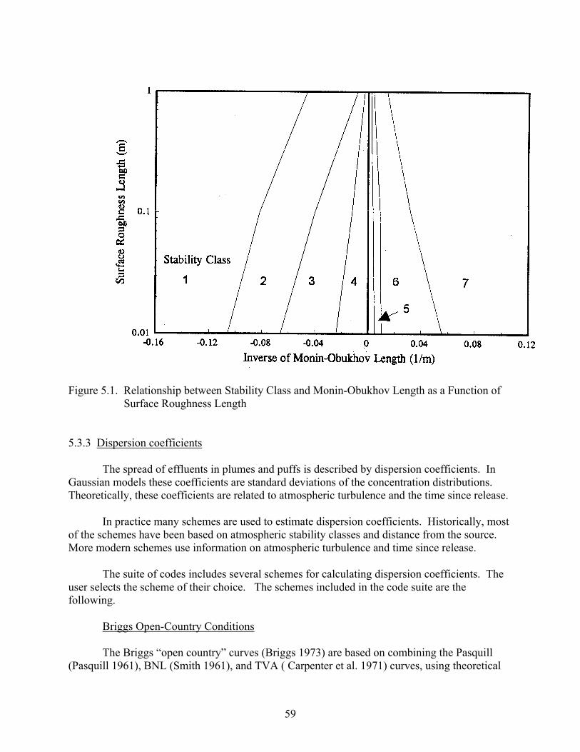
59

Figure 5.1. Relationship between Stability Class and Monin-Obukhov Length as a Function of

Surface Roughness Length

5.3.3 Dispersion coefficients

The spread of effluents in plumes and puffs is described by dispersion coefficients. In Gaussian models these coefficients are standard deviations of the concentration distributions. Theoretically, these coefficients are related to atmospheric turbulence and the time since release.

In practice many schemes are used to estimate dispersion coefficients. Historically, most

of the schemes have been based on atmospheric stability classes and distance from the source. More modern schemes use information on atmospheric turbulence and time since release.

The suite of codes includes several schemes for calculating dispersion coefficients. The user selects the scheme of their choice. The schemes included in the code suite are the following.

Briggs Open-Country Conditions

The Briggs “open country” curves (Briggs 1973) are based on combining the Pasquill (Pasquill 1961), BNL (Smith 1961), and TVA ( Carpenter et al. 1971) curves, using theoretical

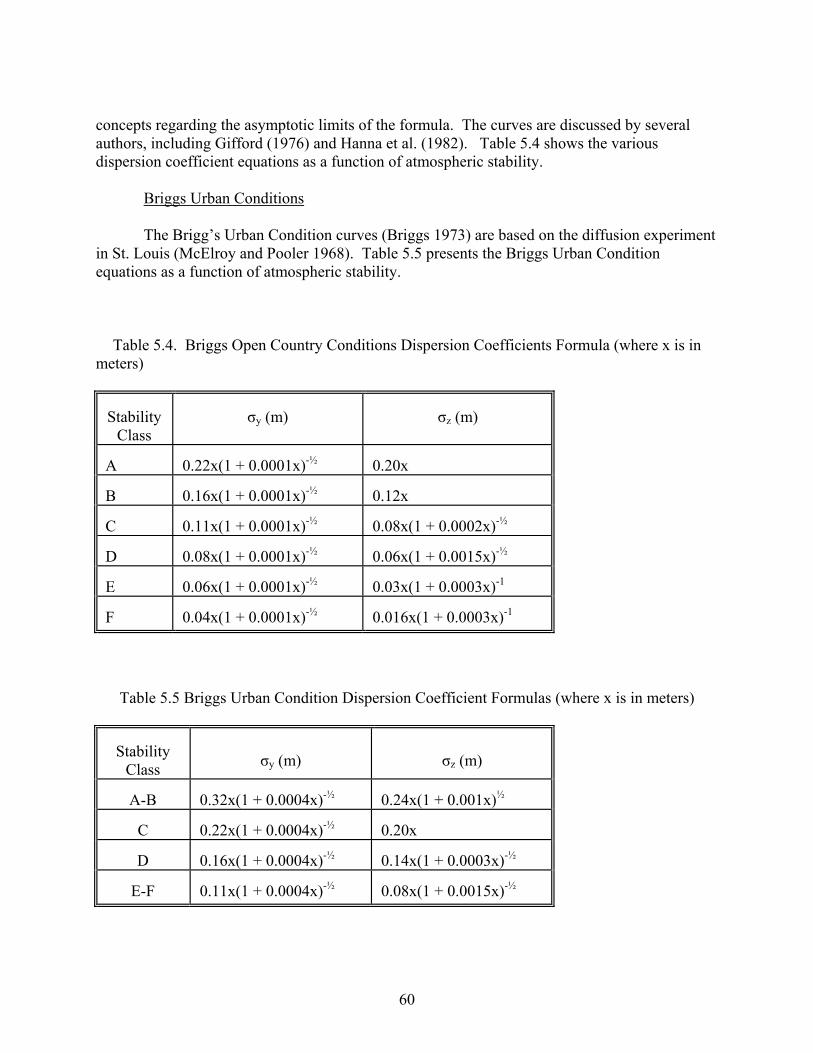
60

concepts regarding the asymptotic limits of the formula. The curves are discussed by several authors, including Gifford (1976) and Hanna et al. (1982). Table 5.4 shows the various dispersion coefficient equations as a function of atmospheric stability.

Briggs Urban Conditions

The Brigg’s Urban Condition curves (Briggs 1973) are based on the diffusion experiment in St. Louis (McElroy and Pooler 1968). Table 5.5 presents the Briggs Urban Condition equations as a function of atmospheric stability.

Table 5.4. Briggs Open Country Conditions Dispersion Coefficients Formula (where x is in meters)

Stability

Class

σy (m) σz (m)

A

0.22x(1 + 0.0001x)-½ 0.20x

B

0.16x(1 + 0.0001x)-½ 0.12x

C

0.11x(1 + 0.0001x)-½ 0.08x(1 + 0.0002x)-½

D

0.08x(1 + 0.0001x)-½ 0.06x(1 + 0.0015x)-½

E

0.06x(1 + 0.0001x)-½ 0.03x(1 + 0.0003x)-1

F

0.04x(1 + 0.0001x)-½ 0.016x(1 + 0.0003x)-1

Table 5.5 Briggs Urban Condition Dispersion Coefficient Formulas (where x is in meters)

Stability

Class

σy (m)

σz (m)

A-B

0.32x(1 + 0.0004x)-½ 0.24x(1 + 0.001x)½

C

0.22x(1 + 0.0004x)-½ 0.20x

D

0.16x(1 + 0.0004x)-½ 0.14x(1 + 0.0003x)-½

E-F

0.11x(1 + 0.0004x)-½ 0.08x(1 + 0.0015x)-½

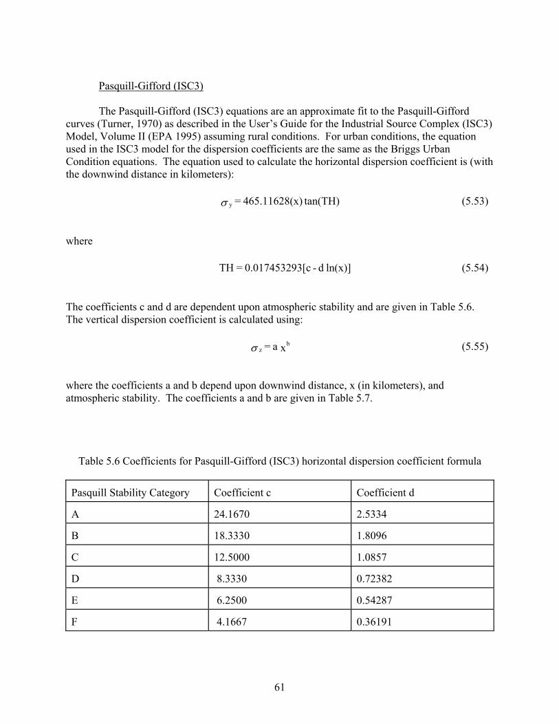
61

Pasquill-Gifford (ISC3)

The Pasquill-Gifford (ISC3) equations are an approximate fit to the Pasquill-Gifford curves (Turner, 1970) as described in the User’s Guide for the Industrial Source Complex (ISC3) Model, Volume II (EPA 1995) assuming rural conditions. For urban conditions, the equation used in the ISC3 model for the dispersion coefficients are the same as the Briggs Urban Condition equations. The equation used to calculate the horizontal dispersion coefficient is (with the downwind distance in kilometers):

where

The coefficients c and d are dependent upon atmospheric stability and are given in Table 5.6. The vertical dispersion coefficient is calculated using:

where the coefficients a and b depend upon downwind distance, x (in kilometers), and atmospheric stability. The coefficients a and b are given in Table 5.7. Table 5.6 Coefficients for Pasquill-Gifford (ISC3) horizontal dispersion coefficient formula Pasquill Stability Category

Coefficient c Coefficient d

A

24.1670 2.5334

B

18.3330 1.8096

C

12.5000 1.0857

D

8.3330 0.72382

E

6.2500 0.54287

F

4.1667 0.36191

tan(TH)x)465.11628( = y (5.53)

ln(x)] d - 3[c0.01745329 = TH (5.54)

x a = bz (5.55)

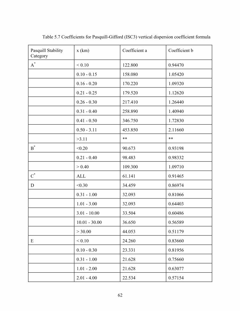
62

Table 5.7 Coefficients for Pasquill-Gifford (ISC3) vertical dispersion coefficient formula Pasquill Stability Category

x (km) Coefficient a

Coefficient b

A*

< 0.10 122.800

0.94470

0.10 - 0.15 158.080

1.05420

0.16 - 0.20 170.220

1.09320

0.21 - 0.25 179.520

1.12620

0.26 - 0.30 217.410

1.26440

0.31 - 0.40 258.890

1.40940

0.41 - 0.50 346.750

1.72830

0.50 - 3.11 453.850

2.11660

>3.11 **

**

B*

<0.20 90.673

0.93198

0.21 - 0.40 98.483

0.98332

> 0.40 109.300

1.09710

C*

ALL 61.141

0.91465

D

<0.30 34.459

0.86974

0.31 - 1.00 32.093

0.81066

1.01 - 3.00 32.093

0.64403

3.01 - 10.00 33.504

0.60486

10.01 - 30.00 36.650

0.56589

> 30.00 44.053

0.51179

E

< 0.10 24.260

0.83660

0.10 - 0.30 23.331

0.81956

0.31 - 1.00 21.628

0.75660

1.01 - 2.00 21.628

0.63077

2.01 - 4.00 22.534

0.57154

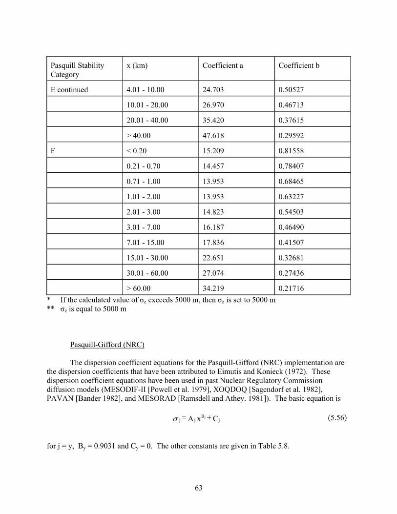
63

Pasquill Stability Category

x (km) Coefficient a

Coefficient b

E continued

4.01 - 10.00 24.703

0.50527

10.01 - 20.00 26.970

0.46713

20.01 - 40.00 35.420

0.37615

> 40.00 47.618

0.29592

F

< 0.20 15.209

0.81558

0.21 - 0.70 14.457

0.78407

0.71 - 1.00 13.953

0.68465

1.01 - 2.00 13.953

0.63227

2.01 - 3.00 14.823

0.54503

3.01 - 7.00 16.187

0.46490

7.01 - 15.00 17.836

0.41507

15.01 - 30.00 22.651

0.32681

30.01 - 60.00 27.074

0.27436

> 60.00 34.219

0.21716

* If the calculated value of σz exceeds 5000 m, then σz is set to 5000 m ** σz is equal to 5000 m

Pasquill-Gifford (NRC)

The dispersion coefficient equations for the Pasquill-Gifford (NRC) implementation are the dispersion coefficients that have been attributed to Eimutis and Konieck (1972). These dispersion coefficient equations have been used in past Nuclear Regulatory Commission diffusion models (MESODIF-II [Powell et al. 1979], XOQDOQ [Sagendorf et al. 1982], PAVAN [Bander 1982], and MESORAD [Ramsdell and Athey. 1981]). The basic equation is

for j = y, By = 0.9031 and Cy = 0. The other constants are given in Table 5.8.

C + x A = jB

jjj (5.56)

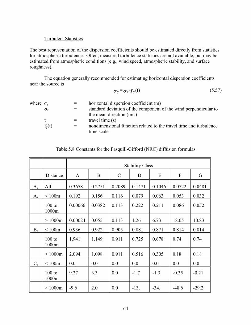
64

Turbulent Statistics The best representation of the dispersion coefficients should be estimated directly from statistics for atmospheric turbulence. Often, measured turbulence statistics are not available, but may be estimated from atmospheric conditions (e.g., wind speed, atmospheric stability, and surface roughness).

The equation generally recommended for estimating horizontal dispersion coefficients near the source is

(t)tf = yvy (5.57)

where σy = horizontal dispersion coefficient (m)

σv = standard deviation of the component of the wind perpendicular to the mean direction (m/s) t = travel time (s) fy(t) = nondimensional function related to the travel time and turbulence time scale.

Table 5.8 Constants for the Pasquill-Gifford (NRC) diffusion formulas

Stability Class

Distance

A

B C D E F

G

Ay

All

0.3658

0.2751 0.2089 0.1471 0.1046 0.0722

0.0481

Az

< 100m

0.192

0.156 0.116 0.079 0.063 0.053

0.032

100 to 1000m

0.00066

0.0382 0.113 0.222 0.211 0.086

0.052

> 1000m

0.00024

0.055 0.113 1.26 6.73 18.05

10.83

Bz

< 100m

0.936

0.922 0.905 0.881 0.871 0.814

0.814

100 to 1000m

1.941

1.149 0.911 0.725 0.678 0.74

0.74

> 1000m

2.094

1.098 0.911 0.516 0.305 0.18

0.18

Cz

< 100m

0.0

0.0 0.0 0.0 0.0 0.0

0.0

100 to 1000m

9.27

3.3 0.0 -1.7 -1.3 -0.35

-0.21

> 1000m

-9.6

2.0 0.0 -13. -34. -48.6

-29.2

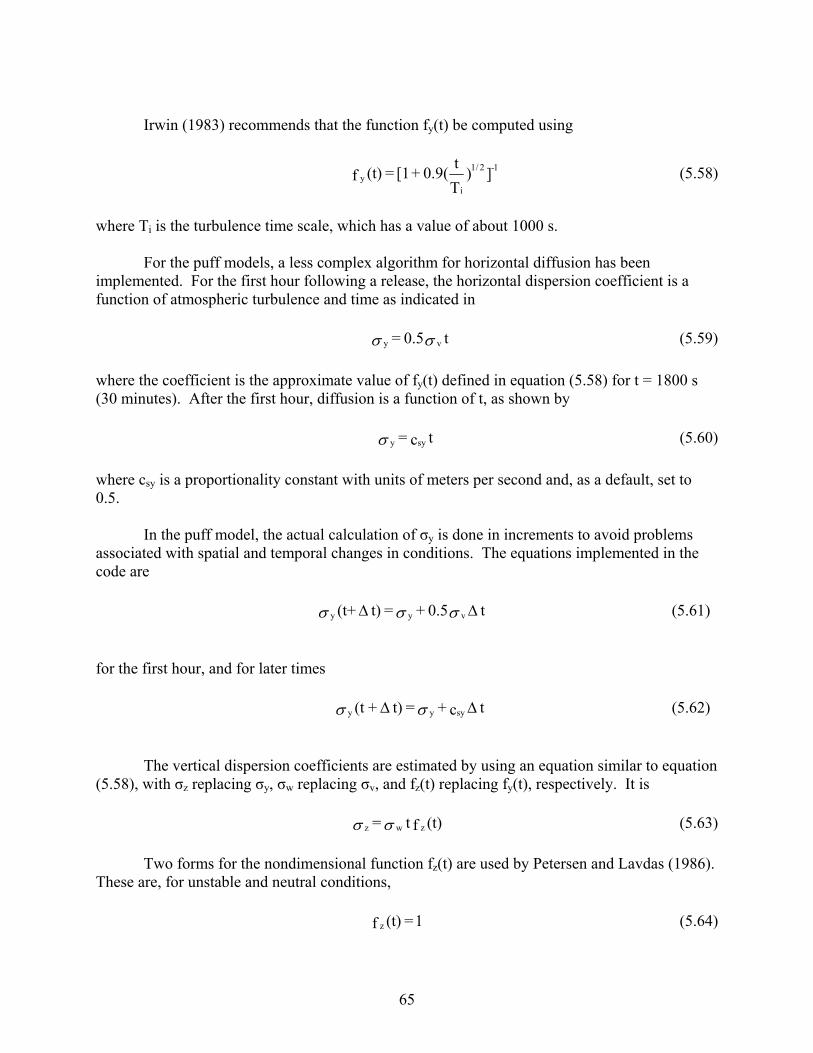
65

Irwin (1983) recommends that the function fy(t) be computed using

])T

t0.9( + [1 = (t)f

1-2/1

iy (5.58)

where Ti is the turbulence time scale, which has a value of about 1000 s.

For the puff models, a less complex algorithm for horizontal diffusion has been implemented. For the first hour following a release, the horizontal dispersion coefficient is a function of atmospheric turbulence and time as indicated in

t0.5 = vy (5.59)

where the coefficient is the approximate value of fy(t) defined in equation (5.58) for t = 1800 s (30 minutes). After the first hour, diffusion is a function of t, as shown by

tc = syy (5.60)

where csy is a proportionality constant with units of meters per second and, as a default, set to 0.5.

In the puff model, the actual calculation of σy is done in increments to avoid problems associated with spatial and temporal changes in conditions. The equations implemented in the code are

for the first hour, and for later times

The vertical dispersion coefficients are estimated by using an equation similar to equation

(5.58), with σz replacing σy, σw replacing σv, and fz(t) replacing fy(t), respectively. It is

(t)ft = zwz (5.63)

Two forms for the nondimensional function fz(t) are used by Petersen and Lavdas (1986). These are, for unstable and neutral conditions,

1 = (t)f z (5.64)

t0.5 + = t)(t+ vyy (5.61)

tc + = t) +(t syyy (5.62)

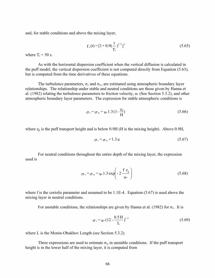
66

and, for stable conditions and above the mixing layer,

])T

t0.9( + [1 = (t)f

1-2/1

iz (5.65)

where Ti = 50 s.

As with the horizontal dispersion coefficient when the vertical diffusion is calculated in the puff model, the vertical dispersion coefficient is not computed directly from Equation (5.63), but is computed from the time derivatives of these equations.

The turbulence parameters, σv and σw, are estimated using atmospheric boundary layer relationships. The relationship under stable and neutral conditions are those given by Hanna et al. (1982) relating the turbulence parameters to friction velocity, u* (See Section 5.3.2), and other atmospheric boundary layer parameters. The expression for stable atmospheric conditions is

where zp is the puff transport height and is below 0.9H (H is the mixing height). Above 0.9H,

For neutral conditions throughout the entire depth of the mixing layer, the expression

used is

where f is the coriolis parameter and assumed to be 1.1E-4. Equation (5.67) is used above the mixing layer in neutral conditions.

For unstable conditions, the relationships are given by Hanna et al. (1982) for σv. It is

)L

H0.5 - (12 u = 3/1

*v (5.69)

where L is the Monin-Obukhov Length (see Section 5.3.2).

Three expressions are used to estimate σw in unstable conditions. If the puff transport height is in the lower half of the mixing layer, it is computed from

)Hz - (1 1.3 u = = p

*wv (5.66)

u 1.3 = = wv (5.67)

u

zf2-exp 1.3 u = =

*

p*wv (5.68)

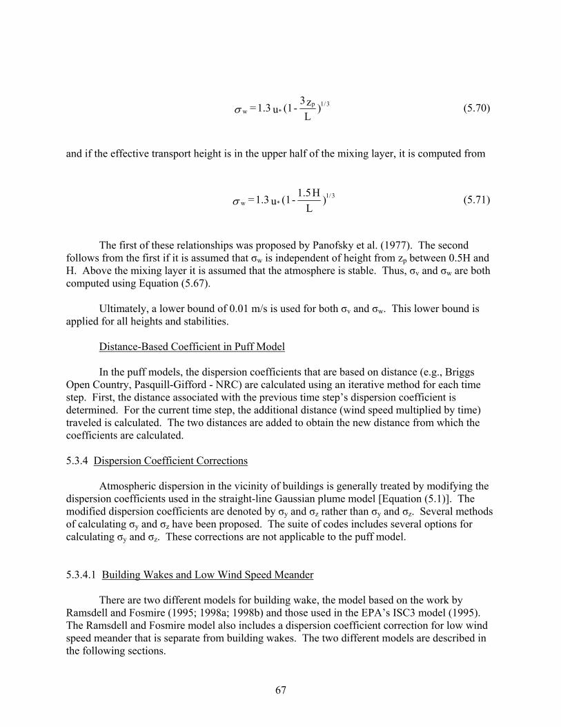
67

and if the effective transport height is in the upper half of the mixing layer, it is computed from

The first of these relationships was proposed by Panofsky et al. (1977). The second

follows from the first if it is assumed that σw is independent of height from zp between 0.5H and H. Above the mixing layer it is assumed that the atmosphere is stable. Thus, σv and σw are both computed using Equation (5.67).

Ultimately, a lower bound of 0.01 m/s is used for both σv and σw. This lower bound is applied for all heights and stabilities.

Distance-Based Coefficient in Puff Model

In the puff models, the dispersion coefficients that are based on distance (e.g., Briggs Open Country, Pasquill-Gifford - NRC) are calculated using an iterative method for each time step. First, the distance associated with the previous time step’s dispersion coefficient is determined. For the current time step, the additional distance (wind speed multiplied by time) traveled is calculated. The two distances are added to obtain the new distance from which the coefficients are calculated. 5.3.4 Dispersion Coefficient Corrections

Atmospheric dispersion in the vicinity of buildings is generally treated by modifying the dispersion coefficients used in the straight-line Gaussian plume model [Equation (5.1)]. The modified dispersion coefficients are denoted by σy and σz rather than σy and σz. Several methods of calculating σy and σz have been proposed. The suite of codes includes several options for calculating σy and σz. These corrections are not applicable to the puff model. 5.3.4.1 Building Wakes and Low Wind Speed Meander

There are two different models for building wake, the model based on the work by Ramsdell and Fosmire (1995; 1998a; 1998b) and those used in the EPA’s ISC3 model (1995). The Ramsdell and Fosmire model also includes a dispersion coefficient correction for low wind speed meander that is separate from building wakes. The two different models are described in the following sections.

)Lz3

- (1 u 1.3 = 3/1p*w (5.70)

)L

H1.5 - (1 u 1.3 = 3/1

*w (5.71)

68

Ramsdell and Fosmire Model

Ramsdell and Fosmire (1995; 1998a; 1998b) suggest that the maximum concentration in

the vicinity of a building can be calculated using

where σy is the usual dispersion coefficient, Δσy1 is a low wind speed correction, and Δσy2 is a high wind speed, wake correction. An identical relationship defines σz. The low-speed corrections are given by

where Ay and Az are constants that depend, in part, on the parameterization used for the normal dispersion coefficients. Table 5.9 contains the constants Ay and Az for the various dispersion coefficient parameterization schemes.

The high speed wake corrections are given by

where By and Bz are constants that depend, in part, on the parameterization chosen for the normal dispersion coefficients and A is the cross-sectional area of the building. In Ramsdell and Fosmire (1998b), it was determined that current open-terrain dispersion parameters already overestimated diffusion in high wind speed conditions. Thus, the constants By and Bz are zero for the various dispersion parameterizations used in these codes.

) + + ( = 2/122

21

2y

2y yy (5.72)

)] U100

xexp(- )

U100

x + 1 ( - 1 [ A =

. )] U1000

xexp(- )

U1000

x + 1 ( - 1 [ A =

z21

y21

z

y

(5.73)

)] A10

x - exp(

A 10

x + 1 ( - 1 [A U B =

)] A10

x - exp(

A 10

x + 1 ( - 1 [A U B =

2z

22

2y

22

z

y

(5.74)

69

Table 5.9. Coefficient for Low Wind Speed Meander Modela

Diffusion Parameterization

Ay Az

Briggs Open Country

5.98 x 105 2.75 x 103

Briggs Urban Condition

2.23 x 105 3.38 x 102

Pasquill-Gifford (ISC3)

6.53 x 105 2.51 x 103

Pasquill-Gifford (NRC)

6.89 x 105 2.35 x 103

Turbulent Statistics

2.07 x 105 1.19 x 103

a. Developed for GENII using the approach of Ramsdell and Fosmire (1995)

EPA’s ISC3 Wake Models

As an alternative to the Ramsdell and Fosmire models, the two plume models allow the user to use the building wake models found in the EPA ISC3 model. The full details of the building wake model can be found in User’s Guide for the Industrial Source Complex (ISC3) Model, Volume II (EPA 1995) and are summarized here.

The ISC3 model uses two different procedures to account for building wake. The first procedure is based on the work of Huber (1977) and Huber and Snyder (1976), and will be referred to as the Huber-Synder building wake. The other procedure follows the suggestions of Schulman and Hanna (1986) based on the work by Scire and Schulman (1980) and will be referred to as the Schulman-Scire building wake. The Schulman-Scire building wake is applied when the stack height is less than the building height plus half the lesser of the building height or width. Otherwise, the Huber-Synder building wake procedure is used. For both procedures, direction-specific building dimension are specified by the user.

Huber - Synder Building Wake

The Huber-Synder building wake procedure is calculated by using a series of steps. The first step is to calculate the transitional plume rise due to momentum (Equation 5.47) at a distance of two building heights. If the effective plume height (with no stack-tip downwash adjustment) is greater than either 2.5 building heights or the sum of the building height and 1.5 times the building width, the plume is assumed to be unaffected by the building wake. Otherwise, the plume is assumed to be affected by the building wake.

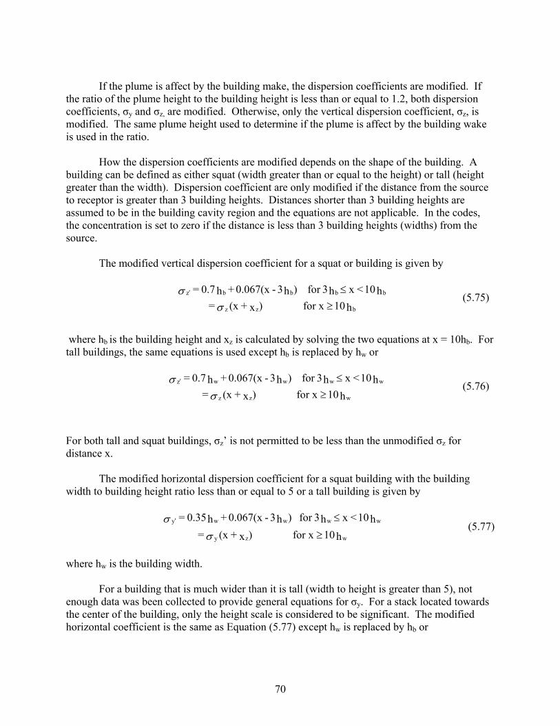
70

If the plume is affect by the building make, the dispersion coefficients are modified. If the ratio of the plume height to the building height is less than or equal to 1.2, both dispersion coefficients, σy and σz, are modified. Otherwise, only the vertical dispersion coefficient, σz, is modified. The same plume height used to determine if the plume is affect by the building wake is used in the ratio.

How the dispersion coefficients are modified depends on the shape of the building. A building can be defined as either squat (width greater than or equal to the height) or tall (height greater than the width). Dispersion coefficient are only modified if the distance from the source to receptor is greater than 3 building heights. Distances shorter than 3 building heights are assumed to be in the building cavity region and the equations are not applicable. In the codes, the concentration is set to zero if the distance is less than 3 building heights (widths) from the source.

The modified vertical dispersion coefficient for a squat or building is given by

where hb is the building height and xz is calculated by solving the two equations at x = 10hb. For tall buildings, the same equations is used except hb is replaced by hw or

For both tall and squat buildings, σz’ is not permitted to be less than the unmodified σz for distance x.

The modified horizontal dispersion coefficient for a squat building with the building width to building height ratio less than or equal to 5 or a tall building is given by

h10for x )x +(x =

h10 < x h3for )h3 -0.067(x +h0.35 =

wzy

wwwwy

(5.77)

where hw is the building width.

For a building that is much wider than it is tall (width to height is greater than 5), not enough data was been collected to provide general equations for σy. For a stack located towards the center of the building, only the height scale is considered to be significant. The modified horizontal coefficient is the same as Equation (5.77) except hw is replaced by hb or

h10for x )x +(x =h10 < x h3for )h3 -0.067(x +h0.7 =

bzz

bbbbz

(5.75)

h10for x )x +(x =h10 < x h3for )h3 -0.067(x +h0.7 =

wzz

wwwwz

(5.76)

71

If the stack is located within about 2.5 building heights from the end of the building, the horizontal dispersion coefficient is calculated using

h10for x )x +(x =

h10 < x h3for )h3 -0.067(x +h1.75 =

bzy

bbbby

(5.79)

The upper bound of the concentration for a squat building with a width to height ratio greater than 5 is given by Equation (5.78), while the lower bound is given by Equation (5.79). The user is given the option to use either the equation that gives the upper or lower bound concentration. By default, the upper bound is used.

Schulman-Scire Building Wake

The Schulman-Scire building wake procedure involves two steps. First, the plume is reduced due to initial plume dilution, and second, the vertical dispersion coefficient is modified. The vertical dispersion coefficient is calculated using either Equation (5.75) or Equation (5.76) depending upon the building dimensions. In addition, a linear decay factor is applied where

where σz’ is from either Equation (5.75) or (5.76) and A is the linear decay factor determined by

L2 + h > h if 0 =A

L2 + h h < h if 1 + L 2h - h =A

h h if 1 =A

bbe

bbebb

eb

be

(5.81)

where he is the height of the plume with transitional momentum rise at 2 building heights downwind.

The plume rise is estimated as follows. The initial dimensions of the downwash plume are approximated by a line source of length Ly and a depth 2Ro where

zyby

zybzyy

bz0

< ,L3 = x 0 = L

,L3 = x ) - ( 2 = L

L3 = x A 2 = R

(5.82)

where Lb is the minimum of the building height and building width and A is a linear decay factor given by Equation (5.81). Both σy and σz are evaluated at x = 3Lb, and are taken as the larger of

h10for x )x +(x =

h10 < x h3for )h3 -0.067(x +h0.35 =

bzy

bbbby

(5.78)

zz A = (5.80)

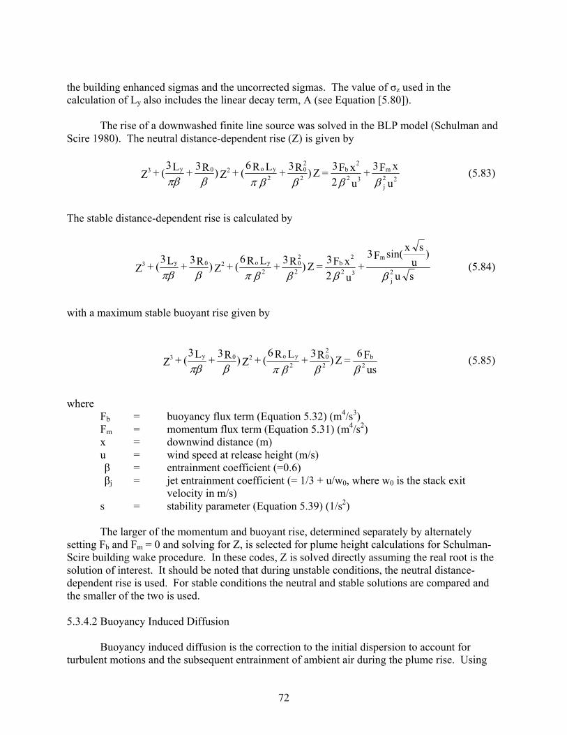
72

the building enhanced sigmas and the uncorrected sigmas. The value of σz used in the calculation of Ly also includes the linear decay term, A (see Equation [5.80]).

The rise of a downwashed finite line source was solved in the BLP model (Schulman and Scire 1980). The neutral distance-dependent rise (Z) is given by

The stable distance-dependent rise is calculated by

with a maximum stable buoyant rise given by

where

Fb = buoyancy flux term (Equation 5.32) (m4/s3) Fm = momentum flux term (Equation 5.31) (m4/s2) x = downwind distance (m) u = wind speed at release height (m/s) β = entrainment coefficient (=0.6) βj = jet entrainment coefficient (= 1/3 + u/w0, where w0 is the stack exit velocity in m/s)

s = stability parameter (Equation 5.39) (1/s2)

The larger of the momentum and buoyant rise, determined separately by alternately setting Fb and Fm = 0 and solving for Z, is selected for plume height calculations for Schulman-Scire building wake procedure. In these codes, Z is solved directly assuming the real root is the solution of interest. It should be noted that during unstable conditions, the neutral distance-dependent rise is used. For stable conditions the neutral and stable solutions are compared and the smaller of the two is used. 5.3.4.2 Buoyancy Induced Diffusion

Buoyancy induced diffusion is the correction to the initial dispersion to account for turbulent motions and the subsequent entrainment of ambient air during the plume rise. Using

u

xF3 +

u2xF3

= Z)R3 + LR6

( + Z)R3 + L3

( + Z 22j

m

32

2b

2

20

2

yo20y3

(5.83)

su

)u

sxsin(F3

+ u2xF3

= Z)R3 + LR6

( + Z)R3 + L3

( + Z 2j

m

32

2b

2

20

2

yo20y3

(5.84)

usF6

= Z)R3 + LR6

( + Z)R3 + L3

( + Z 2b

2

20

2

yo20y3

(5.85)

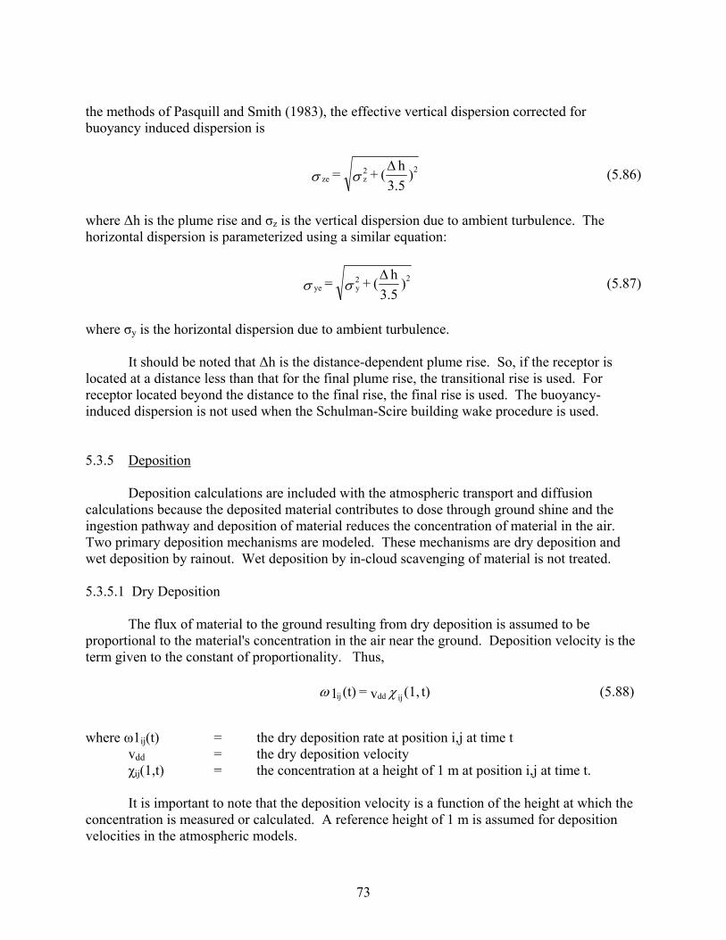
73

the methods of Pasquill and Smith (1983), the effective vertical dispersion corrected for buoyancy induced dispersion is

)3.5

h( + = 22

zze

(5.86)

where Δh is the plume rise and σz is the vertical dispersion due to ambient turbulence. The horizontal dispersion is parameterized using a similar equation:

)3.5

h( + = 22

yye

(5.87)

where σy is the horizontal dispersion due to ambient turbulence.

It should be noted that Δh is the distance-dependent plume rise. So, if the receptor is located at a distance less than that for the final plume rise, the transitional rise is used. For receptor located beyond the distance to the final rise, the final rise is used. The buoyancy-induced dispersion is not used when the Schulman-Scire building wake procedure is used. 5.3.5 Deposition

Deposition calculations are included with the atmospheric transport and diffusion

calculations because the deposited material contributes to dose through ground shine and the ingestion pathway and deposition of material reduces the concentration of material in the air. Two primary deposition mechanisms are modeled. These mechanisms are dry deposition and wet deposition by rainout. Wet deposition by in-cloud scavenging of material is not treated. 5.3.5.1 Dry Deposition

The flux of material to the ground resulting from dry deposition is assumed to be proportional to the material's concentration in the air near the ground. Deposition velocity is the term given to the constant of proportionality. Thus,

where ω1ij(t) = the dry deposition rate at position i,j at time t vdd = the dry deposition velocity χij(1,t) = the concentration at a height of 1 m at position i,j at time t.

It is important to note that the deposition velocity is a function of the height at which the concentration is measured or calculated. A reference height of 1 m is assumed for deposition velocities in the atmospheric models.

t)(1,v = (t)1 ijddij (5.88)

74

Noble gases are inert. The literature contains some discussion of solubility of noble

gases that might lead to deposition on wet surfaces. This deposition is not considered to be significant for dose calculations. As a result, it is assumed that they do not deposit. Therefore, the deposition velocity for noble gases is defined to be zero.

Dry deposition velocities have been calculated from experimental data for particles and gases. In general, the deposition velocities observed for any particular material have a wide range of values. Nevertheless, the deposition velocity is frequently assumed to be constant. More realistically, the dry deposition velocity may be modeled using an analogy to electrical resistance. Resistances are associated with atmospheric conditions, physical and chemical characteristics of the material, and the physical, chemical and biological properties of the surface. Seinfeld (1986) describes the resistance analogy.

For small particles (~ 1 μ ) and gases the resistance model for dry deposition velocities is

)r + r + r( = v-1

tsadd (5.89)

where ra = aerodynamic resistance (s/m)

rs = surface resistance (s/m) rt = transfer resistance (s/m).

The aerodynamic and surface resistances are generally calculated from near surface wind

data. In contrast, the transfer resistance is generally a function of the depositing surface. For example, transfer resistances have been associated with the stomatal openings of plant leaves (Wesley and Hicks 1977).

The aerodynamic resistance is calculated directly from the wind speed and a parameter that is characteristic of the turbulence in the lowest layer of the atmosphere. The usual parameterization for the aerodynamic resistance is

u / U(z)= r *2

a (5.90)

where z = the height at which the concentration is estimated

u* = the characteristic turbulence velocity, called the friction velocity. U(z) = wind speed at height z The concentration is approximately constant for z < 0.2σz as long as x is sufficiently large that σz is greater than or equal to the height of release. Thus, for most elevated release cases, the 10 m wind speed may be used directly in calculating ra.

The surface resistance is only a function of the friction velocity. It is

75

where 2.6 is a dimensionless empirical constant and 0.4 is von Karman’s constant.

The transfer resistance is used as a mathematical device to establish an upper limit on the deposition velocity. The user can enter transfer resistance, but as a default, 10 and 100 s/m are assumed for gas (iodine) and particles, respectively (Ramsdell et al. 1994).

Equation (5.88) is appropriate for small particles where the settling velocity of the particles may be neglected. A gravitational settling term should be added for larger particles when the settling velocity is not negligible. In this case, the deposition velocity is

v + )vrr + r + r + r( = v s-1

ssatsadd (5.92)

where vs is the gravitational settling velocity, which is a function of particle size and density. The settling velocity used in the codes is the same as that for the EPA ISC3 model (EPA 1995) and is given by

18S c d g ) - (

= vCF2

2pAIR

s (5.93)

where ρ = the particle density (g/cm3)

ρAIR = the air density (= 1.2 x 10-3 g/cm3) dp = the particle diameter (μm) μ = the absolute viscosity of air (=1.81 x 10-4 g/cm/s) c2 = air units conversion constant (=1 x 10-8 cm2/μm2) SCF = the slip correction factor, which is computed as

where x2, a1, a2, and a3 are constants with values of 6.5x10-6, 1.257, 0.4, and 0.55x10-4, respectively. 5.3.5.2 Wet Deposition

Wet deposition of gases is treated the same as dry deposition in Equation (5.88) with ω2ij

replacing ω1ij and vdw, a wet deposition velocity, replacing vdd. The model used assumes that the exchange of gas between the air and precipitation is sufficiently rapid that an equilibrium is maintained between the concentrations in the air and in the precipitation. With this assumption, the flux of gas to the surface is proportional to the concentration of the gas in the air at ground level, the precipitation rate, and a solubility coefficient related to the Henry's law constant for

u/6.5 = )u(0.4 / 2.6 = r **s (5.91)

d 10

))x

daexp(- a + a( x2+1 = S

p4-

2

p3212

CF (5.94)

76

the gas. A wet deposition velocity, similar to the dry deposition velocity, combines the precipitation rate and solubility coefficient. It is

where S = the solubility coefficient

Pr = the precipitation rate in mm/hr c = a conversion factor to convert Pr to m/s.

The wet deposition model for gases assumes that the gases are dissolved rapidly by the

precipitation. Implicit in this assumption is the assumption that the precipitation is liquid or at least has a liquid exterior because the rate of exchange of gases between air and ice is sufficiently low to be negligible. As a result, the wet deposition velocity for snow is zero if temperature data are available and the temperature is less than -3°C. If temperature data are not available, the wet deposition velocity is zero for all forms of frozen precipitation.

The wet deposition of particles is modeled using a washout coefficient. This model assumes that the particles are collected by impaction as the precipitation falls through the plume. The model also assumes that the scavenging process is irreversible, i.e. once collected the particles remain with the precipitation. The general model for wet deposition of particles is

where Λ is the washout coefficient. Washout coefficients are assumed to be functions of the type of precipitation (liquid or frozen), the precipitation rate, and the collection efficiency of the precipitation.

For liquid precipitation (rain, drizzle, etc), henceforth referred to as rain, the washout coefficient is calculated by the expression discussed in Slinn (1984), which is

where Λr = the washout coefficient for rain

C = empirical constant with value of 0.5 E = average collection efficiency, assumed to be 1.0 Pr = precipitation rate in mm/hr Pn = normalized precipitation rate (Pr / 1 mm/hr).

During period of frozen precipitation (snow, hail), henceforth referred to as snow, the

washout coefficient will be calculated by

P S c = v rdw (5.95)

dzt)(z, = (t)3 ij0

ij

(5.96)

P 0.35P E C

= n

4/1r

r (5.97)

77

where Λs = the washout coefficient for snow

0.2 = empirical constant with units of mm-1 Pr = the precipitation rate in mm/hr, liquid water equivalent.

The integral in Equation (5.96) can be solved based on equations used to calculate the

concentration, as only the reflection term, G(z), is dependent upon z. If only the first terms of the reflection terms are used, the wet deposition of particles can be estimated as follows.

The sector averaged point and area source for the plume is given by

The non-sector averaged point source for a plume is given by

The non-sector averaged area source for a plume is given by

In the puff model, the washout is calculated by

r

2

r3

2

])r

Qexp[-0.5( =

(5.102)

where Q’ is the release rate corrected for depletetion and decay and Q is the mass of the puff. 5.3.5.3 Total Deposition

Given the dry and wet deposition velocities, the surface contamination that accumulated at any point during the short period is computed as

P 0.2 = rs (5.98)

w3

U

Q =

(5.99)

y

2

y3

U2

])y

exp[-0.5(Q

=

(5.100)

U

)]2

y - aerf( + )

2

y + a[erf( 0.5 Q

= yy3

(5.101)

78

where D(x,y,T) is the total surface contamination (Ci/m2) at position (x,y) and for time period T. The deposition rate, which is calculated in the chronic models, is given by

5.3.6. Radioactive Decay

Both the plume and puff models have been developed to handle in-transit decay. The

decay is based on the general algorithm for radioactive decay with branching found in Strenge (1997). The general solution is given by

where Qi(t) = activity of chain member i at time t λri = radioactive transition rate constant (half-life) for chain member i (s-1) λen = effective lost rate constant for precursor radionuclide n and is given by λen

= Li + λrn where Li is the total rate constant for all physical transfers of chain member i from the medium (s-1)

and Kin is defined by

where dji is the fraction [branching factor] of precursor radionuclide transitions (chain member j) that result in production of the chain member i.

t(t)]3+(t)2+(t)1[ = T)y,D(x, ijijij

T

0

(5.103)

T)y,D(x, T

1 = T)y,(x,D (5.104)

e K = (t)Q t-in

i

1 =n rii

en (5.105)

1r

111

(0)Q = K (5.106)

enei

jnrjji

1 - i

n = jin

-

Kd = 1) - i1 =(n K

(5.107)

K - (0)Q

= K in

1 - i

1 =n ri

iii

(5.108)

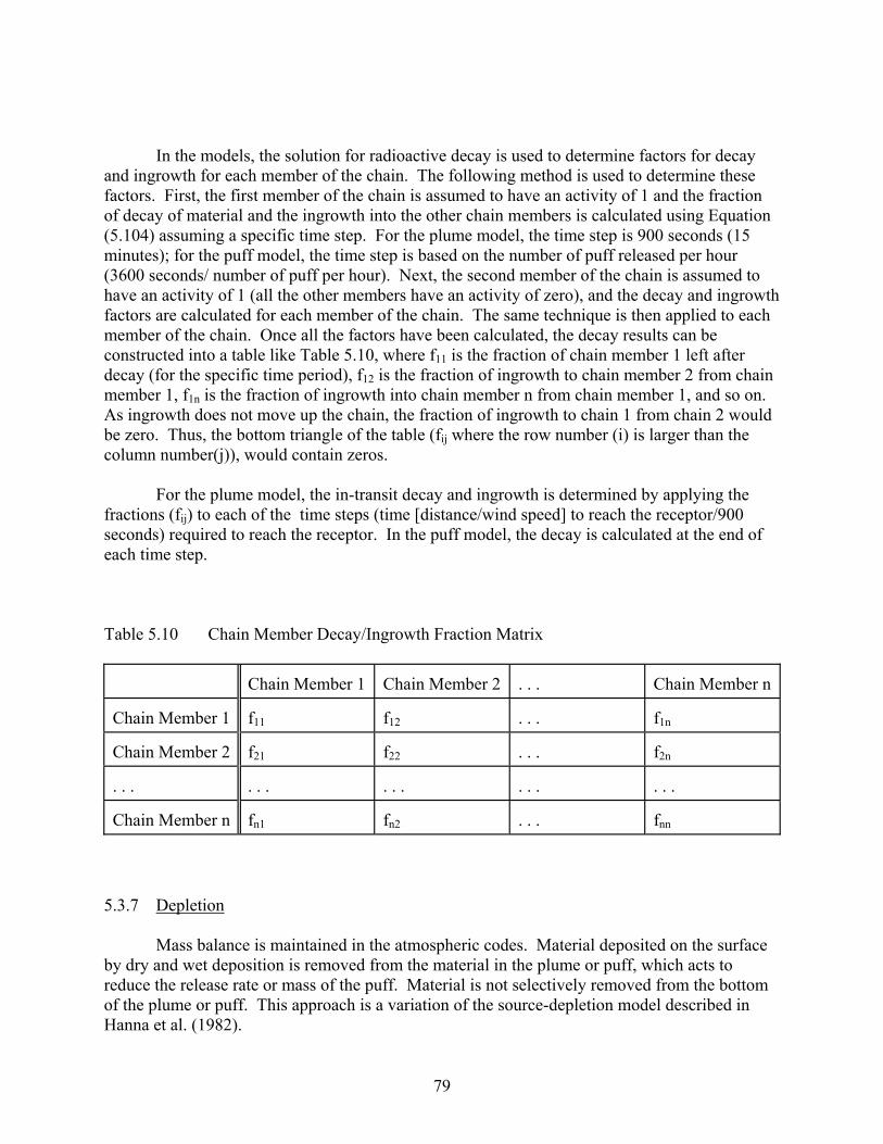
79

In the models, the solution for radioactive decay is used to determine factors for decay

and ingrowth for each member of the chain. The following method is used to determine these factors. First, the first member of the chain is assumed to have an activity of 1 and the fraction of decay of material and the ingrowth into the other chain members is calculated using Equation (5.104) assuming a specific time step. For the plume model, the time step is 900 seconds (15 minutes); for the puff model, the time step is based on the number of puff released per hour (3600 seconds/ number of puff per hour). Next, the second member of the chain is assumed to have an activity of 1 (all the other members have an activity of zero), and the decay and ingrowth factors are calculated for each member of the chain. The same technique is then applied to each member of the chain. Once all the factors have been calculated, the decay results can be constructed into a table like Table 5.10, where f11 is the fraction of chain member 1 left after decay (for the specific time period), f12 is the fraction of ingrowth to chain member 2 from chain member 1, f1n is the fraction of ingrowth into chain member n from chain member 1, and so on. As ingrowth does not move up the chain, the fraction of ingrowth to chain 1 from chain 2 would be zero. Thus, the bottom triangle of the table (fij where the row number (i) is larger than the column number(j)), would contain zeros.

For the plume model, the in-transit decay and ingrowth is determined by applying the fractions (fij) to each of the time steps (time [distance/wind speed] to reach the receptor/900 seconds) required to reach the receptor. In the puff model, the decay is calculated at the end of each time step. Table 5.10 Chain Member Decay/Ingrowth Fraction Matrix

Chain Member 1 Chain Member 2 . . .

Chain Member n

Chain Member 1

f11 f12 . . .

f1n

Chain Member 2

f21 f22 . . .

f2n

. . .

. . . . . . . . .

. . .

Chain Member n

fn1 fn2 . . .

fnn

5.3.7 Depletion

Mass balance is maintained in the atmospheric codes. Material deposited on the surface by dry and wet deposition is removed from the material in the plume or puff, which acts to reduce the release rate or mass of the puff. Material is not selectively removed from the bottom of the plume or puff. This approach is a variation of the source-depletion model described in Hanna et al. (1982).

80

In the atmosphere, deposition results in a mass deficit in the layer of air next to the

surface. Source-depletion models instantaneously propagate this deficit through the full vertical extent of the plume or puff. This propagation is unrealistic, particularly in stable atmospheric conditions. Using the resistance analogy to estimate the deposition velocities does not deal with this problem explicitly. However, using the resistance analogy results in lower deposition velocities during stable conditions, which reduces the magnitude of the error.

For a puff model, the mass from each puff is determined from analytical integration of the deposition flux over the area covered by the puff and computation interval. The mass removed from each puff to account for dry deposition of particles and wet and dry deposition of gases is computed using

where ΔQd is the amount of mass removed and dv is ddd for particles or ddd + ddw for gases.

Substituting the definition of χ from Equation (5.25) and performing the integration, the decrease in material becomes

z

vd

2

tQG(z)d2 = Q

(5.110)

During periods of precipitation, the additional rate of mass loss from a puff by washout of

particles is determined by integrating the washout rate over the area covered by the puff and is calculated as follows

When this integration is carried out, the rate of loss is equal to the product of the mass in the puff and the washout coefficient. Thus,

This loss of mass is distributed throughout the puff.

ddr r d t = Q v

0 =r

2

0 =

d

(5.109)

ddr r 2

)2rexp(- Q

t = Q2r

2r

2

0 =r

2

0 =

w

(5.111)

t)]exp(- - [1 Q = Qw (5.112)

81

In the puff models, depletion is computed at the end of each time step. If there is no precipitation, the mass remaining in the puff is computed assuming only dry deposition as

where i is the puff index and j is the time index. When there is precipitation, the depletion calculation is

For the plume models, a different approach is taken. The depletion of the source term per

unit distance is given by Van der Hoven (1968) as

For a point source, the integral can be solved to give

which can be rearranged as

Solving the integral on the left hand side gives

or

dx)G(z)

U

d

2

2

1exp(- )x(Q = )x(Q

z

x

x

v12

2

1

(5.119)

Q - Q = Q dij1ij+ (5.113)

Q - t)exp(-Q = Q dij1ij+ (5.114)

dyd - = dy y)(x, - = dx

Qdv

--

(5.115)

G(z)U

Qd2

2

1 - =

dx

Qd

z

v

(5.116)

dxG(z)

U

d

2

2

1- =

Q

Qd

z

x

x

vx

x

2

1

2

1

(5.117)

dxG(z)

U

d

2

2

1- =

)x(Q

)x(Qln

z

x

x

v

1

22

1

(5.118)

82

The integral of the reflection term,G(z), and the vertical dispersion coefficient normally can not be solved explicitly. In the codes, the integral is approximated numerically using a simple trapezoidal rule. The integral is calculated at each receptor in the order of closest receptor to the source to farthest receptor from the source. Thus, the depletion for a receptor would be the sum of the depletion at the previous receptor and the Equation (5.119), where x1 is the distance to the previous receptor and x2 is the distance to the current receptor. If the distance between receptors is greater than twice the distance from the previous receptor to the source, depletion is calculated at an intermediate point that is twice the distance from the previous receptor to the source. For example, if the two receptors are at 100 and 500 meters, the depletion at two intermediate points, 200 and 400 meters, would be calculated. The depletion at 500 meters would be the sum of the depletion at 400 meters and Equation (5.119) with x1 = 400 meters and x2 = 500 meters. These intermediate points are calculated to prevent unreasonable errors in the estimation of the integral. To prevent errors in estimating the integral, depletion does not occur for distances less than 100 meters from the source.

At a downwind distance where σz ≥ 1.2 H (e.g., the concentration is uniformly mixed

through the boundary layer), Equation (5.115) can be solved to give

)UH

]x - x[vexp(- )x(Q = )x(Q 12d12 (5.120)

As Equation (5.120) does not involve an integral, at the distances where σz ≥ 1.2H, Equation (5.120) is used to estimate the depletion of the plume. If this distance where σz = 1.2H occurs between two receptors, the depletion is a sum of the depletion calculated by Equation (5.119) up to the distance where σz = 1.2H and Equation (5.120) for the rest of the distance to the second receptor.

For the area source, depletion is assume to not occur until the plume is far enough distance downwind that the area source is similar to a point source (5a for the sector average model and 10a for the non-sector average model). Under this assumption, the equations used for depletion is the same as for a point source (i.e., Equations 5.119 and 5.120). In cases of very large area source, the model tends to underpredict the amount that is depleted. Thus, the concentration and deposition rates would be overpredicted.

For the washout of particles, the integration of deposition term can be solved to give the following

where Δt is (x2 - x1)/U.

)texp(- )x(Q = )x(Q 12 (5.121)

83

5.4 FINITE PLUME SUBMERSION DOSE

Earlier versions of GENII calculated cloud-shine doses using either a semi-infinite cloud model or a finite-plume model based on the model developed for MESORAD (Scherpelz et al. 1986, page 31). The first of these models assumes that activity is uniformly distributed through a large volume, and the second assumes that activity is concentrated in a finite number of points distributed through a volume to represent the actual activity distribution. The use of the semi-infinite cloud model is usually inappropriate in the immediate vicinity of the release point, and application of the MESORAD finite-plume model to cloud-shine dose estimates near the release point did not prove satisfactory. Consequently, the cloud-shine dose models in GENII V.2 have been significantly revised from those used in earlier versions. The basic framework is that also implemented in the RASCAL 3.0 emergency response code (Sjoreen et al. 2001).

Cloud-shine models based on line sources and plane sources have been developed that are analogous to the point-source model used in MESORAD. These models are used, along with the point-source model, until plumes and puffs grow to sufficient size that the assumptions associated with the semi-infinite cloud model are met. In the MESORAD point-source model, point-source dose rates were calculated as a function of distance for each radionuclide from gamma energies. This calculation, which was repetitive and time consuming, has been deleted. The finite-plume cloud-shine models in GENII make use of precalculated dose rate vs distance curves. These curves are provided in the radionuclide data base for each radionuclide for a 1 Ci (0.01 Sv) point source, and a 1 Ci/m (0.01 Sv/m) infinite line source. The remainder of this section describes the GENII V.2 cloud-shine models. 5.4.1 Puff Model Cloud-Shine Dose Calculations

There are three stages in GENII puff-model cloud-shine dose calculations. Near the source where puff dimensions are small compared to the mean path length of photons, GENII uses a revised version of the point-kernel dose model. When the puff radius becomes sufficient (σy=400 m), cloud-shine dose rates beneath the centerline of the plume are calculated using an infinite slab model. The dose rate at ground-level is calculated assuming that the activity in the plume is equally divided among 10 horizontal slabs with slab heights determined by the release height and vertical dispersion coefficients. The change in dose rate with distance from slabs is due only to buildup and absorption of photons; the change in dose rate across the plume is proportional to the crosswind variation of activity concentration in the slab. This model will be discussed further, shortly. Finally, when the vertical dimensions of the plume become sufficient (σz=400 m), cloud-shine is calculated using a semi-infinite cloud model.

The point-kernel integration is based on the formulation of the MESORAD finite-puff cloud shine model (Scherpelz et al., 1986; Ramsdell et al., 1988). This model first calculates composite characteristics (photon energies, photons per disintegration, etc.) of the gamma radiation from the radionuclide mix in a puff. Next, the model calculates the dose rate vs distance from a point source having the composite characteristics using

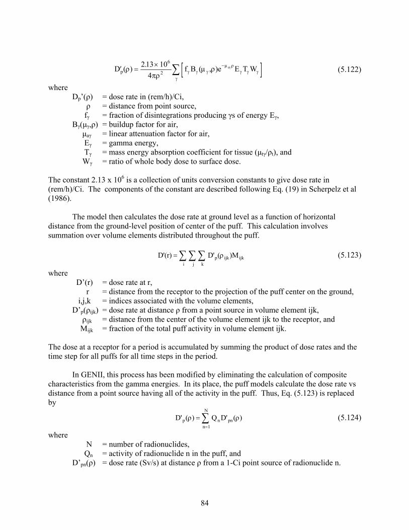
84

D ( ) f B ( , )e E T Wpa

213 10

4

6

2

. (5.122)

where Dp’(ρ) = dose rate in (rem/h)/Ci, ρ = distance from point source, fγ = fraction of disintegrations producing γs of energy Eγ, Bγ(μγ,ρ) = buildup factor for air, μaγ = linear attenuation factor for air, Eγ = gamma energy, Tγ = mass energy absorption coefficient for tissue (μtγ/ρt), and Wγ = ratio of whole body dose to surface dose.

The constant 2.13 x 106 is a collection of units conversion constants to give dose rate in (rem/h)/Ci. The components of the constant are described following Eq. (19) in Scherpelz et al (1986).

The model then calculates the dose rate at ground level as a function of horizontal distance from the ground-level position of center of the puff. This calculation involves summation over volume elements distributed throughout the puff.

D'(r) D' ( )Mp ijkkji

ijk (5.123)

where D’(r) = dose rate at r, r = distance from the receptor to the projection of the puff center on the ground, i,j,k = indices associated with the volume elements, D’p(ρijk) = dose rate at distance ρ from a point source in volume element ijk, ρijk = distance from the center of the volume element ijk to the receptor, and Mijk = fraction of the total puff activity in volume element ijk.

The dose at a receptor for a period is accumulated by summing the product of dose rates and the time step for all puffs for all time steps in the period.

In GENII, this process has been modified by eliminating the calculation of composite characteristics from the gamma energies. In its place, the puff models calculate the dose rate vs distance from a point source having all of the activity in the puff. Thus, Eq. (5.123) is replaced by

D' ( ) Q D' ( )p n pnn

N

1

(5.124)

where N = number of radionuclides, Qn = activity of radionuclide n in the puff, and D’pn(ρ) = dose rate (Sv/s) at distance ρ from a 1-Ci point source of radionuclide n.

85

In the GENII puff models, the puff is divided into ten layers with each layer containing one tenth of the activity. The number of annular rings has been fixed at six, with each ring containing the one sixth of the puff activity, and the number of sectors has been fixed at 12. The fraction of activity in each volume element becomes 1/720 of the total activity. In GENII, then, Eq. (5.124) becomes

D'(r) D' ( ).p ijkkji

1

720 (5.124)

The dose factors are interpolated from tabulated data. Symmetry is used to reduce the computational load.

When the horizontal dispersion parameter reaches 400 m, the puff radius is large enough that the horizontal variations in the cloud shine dose rate are directly proportional to the horizontal variation in concentration in the puff. At this point, MESORAD changed to a semi-infinite cloud model. The GENII puff models change from the point-source based cloud-shine model to a new plane-source based model. The plane-source model assumes that the puff is a vertical cylinder as is done in the point source model. However, rather than assuming that activity is distributed among volume elements, the activity is assumed to be concentrated on 10 horizontal slabs (planes).

To calculate the activity in each slab, first integrate the concentration at the center of the puff (y=0) vertically from the bottom of the puff to the top. This is similar to the integration done in calculating the depletion from wet deposition

nn

/y z y

e

z

n

y y

Q.

r.

hdz

Q.

r

2

05 052

053 2 2

2 2

2

2

exp exp exp (5.125)

where χn is the vertically integrated concentration of radionuclide n at the center of the puff. This concentration is then divided by the number of slabs (10) to get the concentration in each slab.

Within the cylinder, the vertical position of the slabs is determined by the effective release height, the mixing layer thickness, and the vertical dispersion coefficient. When a Gaussian distribution is partitioned so the area under the curve is divided into ten equal parts and the center of mass of each part is determined, these centers of mass fall at ±0.127σ, ±0.385σ, ±0.674σ, ±1.037σ, and ±1.645σ. Using this as a basis, the slab heights are initially estimated as he±0.127σz, he±0.385σz, he±0.674σz, he±1.037σz, and he±1.645σz. The initial heights may lie below ground level or above the top of the mixing layer. Any heights that fall outside these bounds are adjusted to account for reflection by the boundaries. Signs of heights that are negative are changed to positive, and heights (hp) that are above the mixing layer are replaced by 2H-hp.

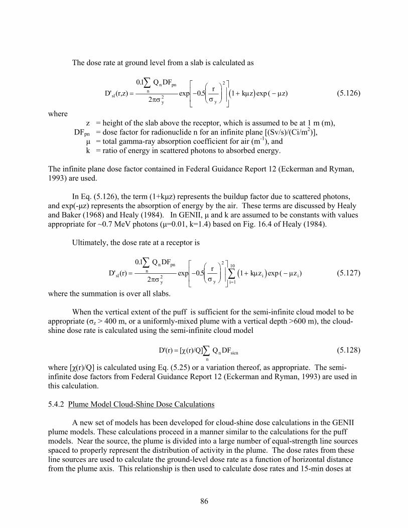
86

The dose rate at ground level from a slab is calculated as

D' (r,z)

. Q DF

.r

k z ( z)sl

n pnn

y y

01

205 1

2

2

exp exp (5.126)

where z = height of the slab above the receptor, which is assumed to be at 1 m (m), DFpn = dose factor for radionuclide n for an infinite plane [(Sv/s)/(Ci/m2)], μ = total gamma-ray absorption coefficient for air (m-1), and k = ratio of energy in scattered photons to absorbed energy.

The infinite plane dose factor contained in Federal Guidance Report 12 (Eckerman and Ryman, 1993) are used.

In Eq. (5.126), the term (1+kμz) represents the buildup factor due to scattered photons, and exp(-μz) represents the absorption of energy by the air. These terms are discussed by Healy and Baker (1968) and Healy (1984). In GENII, μ and k are assumed to be constants with values appropriate for ~0.7 MeV photons (μ=0.01, k=1.4) based on Fig. 16.4 of Healy (1984).

Ultimately, the dose rate at a receptor is

D' (r)

. Q DF

.r

k z ( z )sl

n pnn

y yi i

i

01

205 1

2

2

1

10

exp exp (5.127)

where the summation is over all slabs.

When the vertical extent of the puff is sufficient for the semi-infinite cloud model to be appropriate (σz > 400 m, or a uniformly-mixed plume with a vertical depth >600 m), the cloud-shine dose rate is calculated using the semi-infinite cloud model

D'(r) [ (r)/Q] Q DFn sicnn

(5.128)

where [χ(r)/Q] is calculated using Eq. (5.25) or a variation thereof, as appropriate. The semi-infinite dose factors from Federal Guidance Report 12 (Eckerman and Ryman, 1993) are used in this calculation. 5.4.2 Plume Model Cloud-Shine Dose Calculations

A new set of models has been developed for cloud-shine dose calculations in the GENII plume models. These calculations proceed in a manner similar to the calculations for the puff models. Near the source, the plume is divided into a large number of equal-strength line sources spaced to properly represent the distribution of activity in the plume. The dose rates from these line sources are used to calculate the ground-level dose rate as a function of horizontal distance from the plume axis. This relationship is then used to calculate dose rates and 15-min doses at

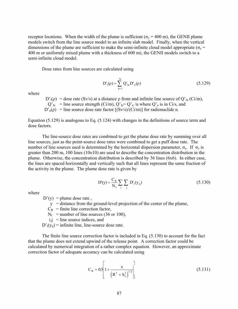
87

receptor locations. When the width of the plume is sufficient (σy = 400 m), the GENII plume models switch from the line source model to an infinite slab model. Finally, when the vertical dimensions of the plume are sufficient to make the semi-infinite cloud model appropriate (σz = 400 m or uniformly mixed plume with a thickness of 600 m), the GENII models switch to a semi-infinite cloud model.

Dose rates from line sources are calculated using

D' ( ) Q' D' ( )ln

N

n ln

1

(5.129)

where D’l(ρ) = dose rate (Sv/s) at a distance ρ from and infinite line source of Q’ln (Ci/m), Q’ln = line source strength (Ci/m), Q’ln= Q’n /u where Q’n is in Ci/s, and D’n(ρ) = line source dose rate factor [(Sv/s)/(Ci/m)] for radionuclide n.

Equation (5.129) is analogous to Eq. (5.124) with changes in the definitions of source term and dose factors.

The line-source dose rates are combined to get the plume dose rate by summing over all line sources, just as the point-source dose rates were combined to get a puff dose rate. The number of line sources used is determined by the horizontal dispersion parameter, σy. If σy is greater than 200 m, 100 lines (10x10) are used to describe the concentration distribution in the plume. Otherwise, the concentration distribution is described by 36 lines (6x6). In either case, the lines are spaced horizontally and vertically such that all lines represent the same fraction of the activity in the plume. The plume dose rate is given by

D'(y)C

ND' (y )R

ll ij

ji

(5.130)

where D’(y) = plume dose rate , y = distance from the ground-level projection of the center of the plume, CR = finite line correction factor, Nl = number of line sources (36 or 100), i,j = line source indices, and D’l(yij) = infinite line, line-source dose rate.

The finite line source correction factor is included in Eq. (5.130) to account for the fact

that the plume does not extend upwind of the release point. A correction factor could be calculated by numerical integration of a rather complex equation. However, an approximate correction factor of adequate accuracy can be calculated using

C .

x

R hR

e

05 12 2 1/2

(5.131)

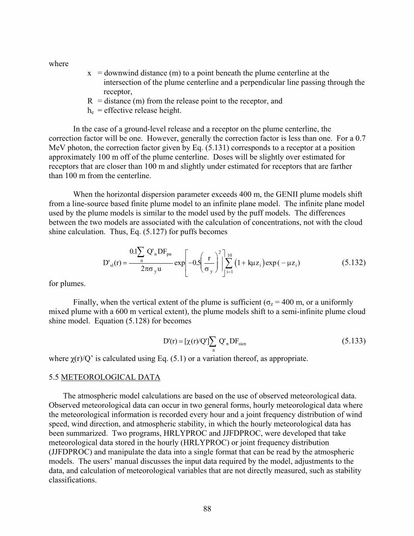
88

where x = downwind distance (m) to a point beneath the plume centerline at the

intersection of the plume centerline and a perpendicular line passing through the receptor,

R = distance (m) from the release point to the receptor, and he = effective release height.

In the case of a ground-level release and a receptor on the plume centerline, the

correction factor will be one. However, generally the correction factor is less than one. For a 0.7 MeV photon, the correction factor given by Eq. (5.131) corresponds to a receptor at a position approximately 100 m off of the plume centerline. Doses will be slightly over estimated for receptors that are closer than 100 m and slightly under estimated for receptors that are farther than 100 m from the centerline.

When the horizontal dispersion parameter exceeds 400 m, the GENII plume models shift from a line-source based finite plume model to an infinite plane model. The infinite plane model used by the plume models is similar to the model used by the puff models. The differences between the two models are associated with the calculation of concentrations, not with the cloud shine calculation. Thus, Eq. (5.127) for puffs becomes

D' (r)

. Q' DF

u.

rk z ( z )sl

n pnn

y yi i

i

01

205 1

2

1

10

exp exp (5.132)

for plumes.

Finally, when the vertical extent of the plume is sufficient (σz = 400 m, or a uniformly mixed plume with a 600 m vertical extent), the plume models shift to a semi-infinite plume cloud shine model. Equation (5.128) for becomes

D'(r) [ (r)/Q'] Q' DFn sicnn

(5.133)

where χ(r)/Q’ is calculated using Eq. (5.1) or a variation thereof, as appropriate. 5.5 METEOROLOGICAL DATA

The atmospheric model calculations are based on the use of observed meteorological data. Observed meteorological data can occur in two general forms, hourly meteorological data where the meteorological information is recorded every hour and a joint frequency distribution of wind speed, wind direction, and atmospheric stability, in which the hourly meteorological data has been summarized. Two programs, HRLYPROC and JJFDPROC, were developed that take meteorological data stored in the hourly (HRLYPROC) or joint frequency distribution (JJFDPROC) and manipulate the data into a single format that can be read by the atmospheric models. The users’ manual discusses the input data required by the model, adjustments to the data, and calculation of meteorological variables that are not directly measured, such as stability classifications.

89

5.6 REFERENCES FOR SECTION 5 Bander, T.J. 1982. PAVAN: An Atmospheric Dispersion Program for Evaluating Design Basis Accidental Releases of Radioacitve Materials from Nuclear Power Stations. NUREG/CR-2858, U.S. Nuclear Regulatory Commission, Washington D.C. Briggs, G.A. 1969. Plume Rise. TID-25075, U.S. Atomic Energy Commission, Washington, D.C. Briggs, G.A. 1972. “Discussion of chimney plumes in neutral and stable surroundings.” Atmospheric Environment 6:507-510. Briggs, G.A. 1973. Diffusion Estimation for Small Emissions. ATDL Contribution File No. 79. Atmospheric Turbulence and Diffusion Laboratory, NOAA, P.O. Box E, Oak Ridge, TN. Briggs, G.A. 1975. “Plume Rise Predictions.” Lectures on Air Pollution and Environmental Impact Analyses, American Meteorological Society, Boston, Massachusetts, pp. 59-111. Briggs, G.A. 1984. “Plume Rise and Buoyancy Effects.” Atmospheric Science and Power Production, DOE/TIC-27601, U.S. Department of Energy, Washington, D.C., pp. 327-366. Businger, J.A., J.C. Wyngaard, Y. Izumi, and E.F. Bradley. 1971. “Flux-Profile Relationships in the Atmospheric Surface Layer.” Journal of the Atmospheric Sciences 28(2):181-189. Carpenter, S.B., T.L. Montgomery, J.M. Leavitt, W.C. Colbaugh, and F.W. Thomas. 1971. “Principal plume dispersion model: TVA power plants.” Journal of the Air Pollution Control Association 23:491-495. Droppo, J.G., Jr. 2007. "Directional Frequency Correction for the Star Meteorological Joint Frequency Computer Program ." Health Physics 93(2):151-156. Eckerman, K.F., and J.C. Ryman. 1993. Federal Guidance Report No. 12. External Exposure to Radionuclides in Air, Water, and Soil. U.S. Environmental Protection Agency, Washington, DC. Eimutis, E.C. and M.G. Konicek. 1972. “Derivations of Continuous Functions for the Lateral and Vertical Atmospheric Dispersion Coefficients.” Atmospheric Environment 6:859-863. EPA (U.S. Environmental Protection Agency). 1995. User’s Guide for the Industrial Source Complex (ISC3) Dispersion Models Volume II - Description of Model Algorithms. EPA-454/B-95-003b. Research Triangle Park, North Carolina. Gifford, F.A. 1976. “Turbulent Diffusion Typing Schemes - a Review.” Nuclear Safety 17:68-86. Golder, D. 1982. “Relations Among Stability Parameters in the Surface Layer.” Boundary-Layer Meteorology 3(1):47-58.

90

Hanna, S.R., G.A. Briggs, and R.P. Hosker. 1982. Handbook on Atmospheric Diffusion. DOE/TIC-11223, U.S. Department of Energy, Washington, D.C. Healy, J.W., and R.E. Baker. 1968. “Radioactive Cloud Dose Calculations.” Meteorology and Atomic Energy 1968. D. Slade, Ed. TID-24190, U.S. Atomic Energy Agency, Washington, DC. Healy, J.W. 1984. “Radioactive Cloud-Dose Calculations.” Atmospheric Science and Power Production, D. Randerson, Ed., DOE/TIC-27601, U.S. Department of Energy, Washington, DC. Huber, A.H. 1977. “Incorporating Building/Terrain Wake Effects on Stack Effluents.” Preprint Volume for the Joint Conference on Applications of Air Pollution Meteorology, American Meteorological Society, Boston, Massachusetts. Huber, A.H. and W.H. Synder. 1976. “Building Wake Effects on Short Stack Effluents.” Preprint Volume for the Third Symposium on Atmospheric Diffusion and Air Quality, American Meteorological Society, Boston, Massachusetts. Irwin, J.S. 1983. “Estimating Plume Dispersion - A Comparison of Several Sigma Schemes.” Journal of Climate and Applied Meteorology 22(1):92-114. McElroy, J.L. and F. Pooler. 1968. The St. Louis Dispersion Study. U.S. Public Heath Service, National Air Pollution Control Administration, Report AP-53. Monin, A.S. and A.M. Obukhov. 1954. “Basic Laws of Turbulent Mixing in the Ground Layer of the Atmosphere.” Trans. Geophys, Inst. Akad. Nauk, USSR 151:163-187. Panofsky, H.A., H. Tennekes, D.H. Lenschow, and J.C. Wyngaard. 1977. “The Characteristics of Turbulent Velocity Components in the Surface Layer Under Convective Conditions.” Boundary-Layer Meteorology 11(3):55-261. Panofsky, H.A. and J.A. Dutton. 1984. Atmospheric Turbulence. J. Wiley & Sons, New York. Pasquill, F. 1961. “The Estimation of the Dispersion of Windborn Material.” The Meteorological Magazine 90:33-49. Pasquill, F. and F. B. Smith. 1983. Atmospheric Diffusion, 3rd Edition. Halsted Press, New York. Paulson, C.A. 1970. “The Mathematical Representation of Wind Speed and Temperature Profiles in the Unstable Atmospheric Surface Layer.” Journal of Applied Meteorology 9(6):857-861.

91

Peterson, W.B. and L.G. Lavdas. 1986. INPUFF 2.0 - A Multiple Source Gaussian Puff Dispersion Algorithm: User’s Guide. EPA-600/8-86/024, Atmospheric Sciences Research Laboratory, U.S. Environmental Protection Agency, Research Triangle Park, North Carolina. Powell, D.C., H.L. Wegley, and T.D. Fox. 1979. MESODIF-II: A Variable Trajectory Plume Segment Model to Assess Ground-Level Air Concentrations and Deposition of Effluent Releases from Nuclear Power Facilities. NUREG/CR-0523, U.S. Nuclear Regulatory Commission, Washington D.C. Ramsdell, J.V., Jr. and G.F. Athey. 1981. MESOI: An Interactive Lagrangian Trajectory Puff Diffusion Model. PNL-3998, Pacific Northwest National Laboratory, Richland, Washington. Ramsdell, J.V., Jr., et al. 1988. The MESORAD Dose Assessment Model, Volume 2: Computer Code. NUREG/CR-4000, Vol. 2, U.S. Nuclear Regulatory Commission, Washington, DC. Ramsdell, J.V., Jr., C.A. Simonen, and K.W. Burk. 1994. Regional Atmospheric Transport Code for Hanford Emission Tracking (RATCHET). PNWD-2224 HEDR, Pacific Northwest National Laboratories, Richland, Washington. Ramsdell, J.V., Jr. and C.J. Fosmire. 1995. Atmospheric Dispersion Estimates in the Vicinity of Buildings. PNL-10286. Pacific Northwest National Laboratories, Richland, Washington. Ramsdell, J.V., Jr. and C.J. Fosmire. 1998a. “Estimating Concentrations in Plumes Released in the Vicinity of Buildings: Model Development.” Atmospheric Environments 32(10):1663-1677. Ramsdell, J.V., Jr. and C.J. Fosmire. 1998b. “Estimating Concentrations in Plumes Released in the Vicinity of Buildings: Model Evaluation.” Atmospheric Environment 32(10):1679-1689. Sagendorf, J.F., J.T. Goll, and W.F. Sandusky. 1982. XOQDOQ: Computer Program for the Meteorological Evaluation of Routine Effluent Releases from Nuclear Power Stations. NUREG/CR-2919, U.S. Nuclear Regulatory Commission, Washington D.C. Scherpelz, R.I. et al. 1986. The MESORAD Dose Assessment Model, Volume 1. NUREG/CR-4000, Vol. 1, U.S. Nuclear Regulatory Commission, Washington, DC. Schulman, L.L. and S.R. Hanna. 1986. “Evaluation of Downwash Modifications to the Industrial Source Complex Model.” Journal of the Air Pollution Control Association 36(3):258-264. Schulman, L.L. and J.S. Scire. 1980. Buoyant Line and Point Source (BLP) Dispersion Model User’s Guide. Document P-7304B, Environmental Research and Technology, Inc., Concord, MA Scire, J.S. and L.L. Schulman. 1980. “Modeling Plume Rise from Low-Level Buoyant Line and Point Sources.” Proceedings Second Joint Conference on Applications of Air Pollution Meteorology, 24-28 March, New Orleans, Louisiana. pp. 133-139.

92

Seinfeld, J.H. 1986. Atmospheric Chemistry and Physics of Air Pollution. John Wiley & Sons, New York. Sjoreen, A.L., J.V. Ramsdell, Jr., T.J. McKenna, S.A. McGuire, C. Fosmire, and G.F. Athey. 2001. RASCAL 3.0: Description of Models and Methods, NUREG-1741, U.S. Nuclear Regulatory Commission, Washington, DC. Skibin, D. and J.A. Businger. 1985. “The Vertical Extent of the Log-Linear Wind Profile Under Stable Stratification.” Atmospheric Environment 19(1):27-30. Slinn, W.G. N. 1984. “Precipitation Scavenging.” In Atmospheric Science and Power Production. D. Randerson, ed., DOE/TIC-27601, U.S. Department of Energy, Washington D.C., pp. 466-532. Smith, F.B. 1961. “An Analysis of Vertical Wind-fluctuation at Heights between 500 and 5,000 Feet.” Quarterly Journal of the Royal Meteorological Society 87(372):180-193. Strenge, D.L. 1997. “A General Algorithm for Radioactive Decay with Branching and Loss from a Medium.” Health Physics 73(6):953-957. Turner, D.B. 1970. Workbook of Atmospheric Dispersion Estimates. PHS Publication No. 999-AP-26. U.S. Department of Health, Education and Welfare, National Air Pollution Control administration, Cincinnati, Ohio. Van der Hoven, I. 1968. “Deposition of Particles and Gases.” In Meteorology and Atomic Energy. D.H. Slade, Ed., TID-24190, U.S. Atomic Energy Commission, Washington D.C., pp. 202-222. Wesley, M.L. and B.B. Hicks. 1977. “Some Factors that Affect the Deposition Rates of Sulfur Dioxide and Similar Gases on Vegetation.” Journal of the Air Pollution Control Association 27:1110-1116.

93

6.0 SURFACE WATER TRANSPORT MODULE The surface water module is included to represent transport through surface waters to the terrestrial environment. The surface water models included in GENII-V2 are described in this section. They are the same as those implemented in GENII Version 1.485 (Napier et al. 1988) and are the same as those employed in the LADTAP II computer program (Strenge, Peloquin, and Whelan 1986). All surface water transport models are based on work of Whelan as described in a report by Codell, Key, and Whelan (1982). Surface water transport models are included for estimating the water concentration resulting from acute and chronic release to non-tidal rivers, and chronic releases to near-shore lake environments. Non-tidal rivers are freshwater bodies with unidirectional flow in definable channels. Near-shore lake environments are surface water areas that are near the shores of large open bodies of water and that have a straight shoreline, constant depth, and steady-state, unidirectional flow parallel to the shore. 6.1 RIVER TRANSPORT MODELS River transport models include representation of acute releases and chronic releases. Acute releases are those resulting from short-term events that release radionuclides over a period of a few hours or days. Chronic releases are continuous and constant releases over periods of weeks to years. The surface water program solves for radionuclide concentrations in a river or large lake under the following limiting assumptions (Codell, Key, and Whelan 1982): · constant flow depth · constant downstream or alongshore velocity · straight river channel · constant lateral dispersion coefficient · continuous point discharge release of effluent · constant river width. Codell, Key, and Whelan (1982) note that applications of models similar to those described here should be restricted to those portions of the near-shore zone of a river or lake that are removed from the influence of the discharge. Initial dilution near the point of discharge is usually controlled by the momentum effects of jets. For non-tidal rivers, the assumed release point is on the near shore of the river with the water usage point (e.g. water treatment plant intake) located at a downstream distance x and a laterally offshore distance y. The water concentration (steady-state) at the downstream location is given by the following equation (NRC 1977; Codell, Key and Whelan 1982):

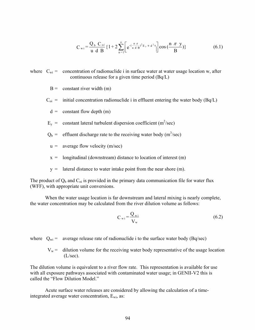
94

where Cwi = concentration of radionuclide i in surface water at water usage location w, after

continuous release for a given time period (Bq/L) B = constant river width (m) Coi = initial concentration radionuclide i in effluent entering the water body (Bq/L) d = constant flow depth (m) Ey = constant lateral turbulent dispersion coefficient (m2/sec) Qb = effluent discharge rate to the receiving water body (m3/sec) u = average flow velocity (m/sec) x = longitudinal (downstream) distance to location of interest (m) y = lateral distance to water intake point from the near shore (m). The product of Qb and Coi is provided in the primary data communication file for water flux (WFF), with appropriate unit conversions. When the water usage location is far downstream and lateral mixing is nearly complete, the water concentration may be calculated from the river dilution volume as follows:

where Qwi = average release rate of radionuclide i to the surface water body (Bq/sec) Vw = dilution volume for the receiving water body representative of the usage location

(L/sec). The dilution volume is equivalent to a river flow rate. This representation is available for use with all exposure pathways associated with contaminated water usage; in GENII-V2 this is called the “Flow Dilution Model.” Acute surface water releases are considered by allowing the calculation of a time-integrated average water concentration, Ewi, as:

)}B

y n ( cos e 2 + 1 {

B du C Q

= C xdu E )B du

n ( -

1 =n

o b i w

2 y

2

i (6.1)

V

Q = C

w

i wi w (6.2)

95

where Ewi = time-integrated average water concentration at water usage location i for radionuclide i (Bq/L)

qwi(t)= instantaneous release rate of radionuclide i to water as a function of time, t,

(Bq/sec) Tw = period over which the release to water occurs for water usage location w (yr), 3.1688E-8 = unit conversion factor (yr/sec), and other terms are as previously defined. The instantaneous release rate is given in the primary data communication file for release to the surface water (WFF) as a function of time. The data for the time points is integrated and averaged over the release period to estimate a value for the average release rate, Qwi. 6.2 NEAR-SHORE LAKE TRANSPORT MODELS Near-shore lake environments are described by a model similar to the river model. The NRC (1977) has suggested use of a quasi-steady-state model valid for simulating contaminant transport in near-shore lake environments for distances up to 16 miles (27 km). The model is represented by the following equation:

where Ez = vertical turbulent dispersion coefficient (m2/sec) z = depth of user’s water intake (m), Coi = initial concentration radionuclide i in effluent entering the water body (Bq/L),

(effluents are assumed to be released at the water surface) d = constant long-shore flow depth (m) Ey = constant lateral turbulent dispersion coefficient (m2/sec) u = average flow velocity (m/sec) x = longitudinal (long-shore) distance to location of interest (m)

V T

Q 8E-3.1688 = t d

V

(t)q

T

8E-3.1688 = E

w

i wi wT

0wi w

w

(6.3)

e e E E x

Q C = C E x 4

u )z - d i (2 -

+

- = i

E x 4

u y -

z y

b i o i w z

2

y

2

(6.4)

96

y = lateral (off-shore) distance to water intake point from the near shore (m). and other terms are as previously defined. Equations (6.1) and (6.4) require values for the lateral and vertical dispersion coefficients. Dispersion coefficients should be obtained by site-specific tracer studies whenever possible. Accurately defining dispersion coefficients for all river or lake environments under all conditions is difficult, if not impossible at this time. However, rough estimates can be defined. The coefficients are defined such that representative properties of the water body are considered when making estimates. In the absence of site-specific estimates of dispersion coefficients Strenge, Peloquin, and Whelan (1986) have suggested use of the following expressions:

and

Even though Equations (6.5) and (6.6) were developed for rivers, they are also suggested for use with near-shore lake environments. 6.4 IMPOUNDMENT MODELS

The GENII Surface Water module includes the hydrodynamic models for reconcentration of radionuclides in reactor cooling ponds – the plug flow, completely mixed, and partially mixed approaches. The equations for plug-flow pond, fully-mixed pond, and partially-mixed pond are given in Section 4.2.3 of Napier (1995). These models are used to modify the discharge from the source into the subsequent river or lake.

The plug flow pond receives the plant effluent and in turn discharges it to a larger body of receiving water. The water does not recirculate back to the plant once it is discharged. Plug flow ponds are usually narrow and well-diked, forcing the plant effluent to travel a well-defined path from the plant discharge point to the point of outfall from the pond. Note, that for a pond of this nature, the travel time t from plant outfall to pond outlet is t = V / qb, where V is the volume of the pond and qb is the reactor discharge rate = the pond outflow rate. The model predicts the radionuclide concentration at the outlet of the pond to be

where V = the effective volume of the pond (m3);

qb = the pond outflow rate (m/yr);

u d 0.06 = Ey (6.5)

u d 0.0059 = Ez (6.6)

. ) q / V - exp( q

W = C b

b

(6.7)

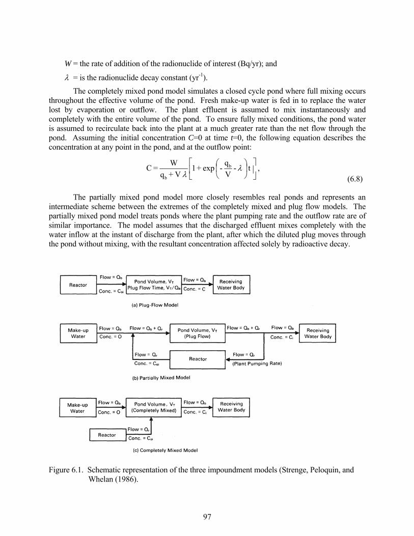
97

W = the rate of addition of the radionuclide of interest (Bq/yr); and

= is the radionuclide decay constant (yr-1).

The completely mixed pond model simulates a closed cycle pond where full mixing occurs throughout the effective volume of the pond. Fresh make-up water is fed in to replace the water lost by evaporation or outflow. The plant effluent is assumed to mix instantaneously and completely with the entire volume of the pond. To ensure fully mixed conditions, the pond water is assumed to recirculate back into the plant at a much greater rate than the net flow through the pond. Assuming the initial concentration C=0 at time t=0, the following equation describes the concentration at any point in the pond, and at the outflow point:

The partially mixed pond model more closely resembles real ponds and represents an intermediate scheme between the extremes of the completely mixed and plug flow models. The partially mixed pond model treats ponds where the plant pumping rate and the outflow rate are of similar importance. The model assumes that the discharged effluent mixes completely with the water inflow at the instant of discharge from the plant, after which the diluted plug moves through the pond without mixing, with the resultant concentration affected solely by radioactive decay.

Figure 6.1. Schematic representation of the three impoundment models (Strenge, Peloquin, and Whelan (1986).

, t - V

q - exp + 1

V + q

W = C b

b

(6.8)

98

Then the concentration at the plant inlet is added to the radioactivity discharged from the plant as the coolant water cycles through. The concentration at the outlet of the pond is given as

,

q - )q+ q(

V exp )q + q(

W = C

pPb

pb

(6.9)

where qp = the discharge flow rate of the plant and qb = the outflow rate of the pond. This equation must be modified for solution of decay chains. The equation may be expanded in an infinite series so that the amount exiting the pond, into the river or lake, is described as:

pb qq

Vn

n

n bb

p

bp

bb e

qq

q

qq

qWqCQSWR

1

1 )( (6.10)

This equation may be solved using the GENII chain decay processor as described in Section 6.3.

6.3 DECAY IN TRANSIT All radionuclides are allowed to undergo chain decay and ingrowth of progeny during the time of transit from the release point to the exposure point as follows.

where Cri(Tyr)= average annual water concentration for radionuclide i at recreational water usage location r (Bq/L)

Crwi(Tyr) = average annual water concentration for radionuclide i evaluated at the

recreational usage location r, but uncorrected for decay in transit from the release point (Bq/L)

Ttr = travel time from water release point to recreational water usage location r (y) Tyr = one year averaging period (y) i = radiological decay constant for radionuclide i (y-1) Decay is handled using the decay processor described in Appendix C.

exp )T( C = )T( C Tt -yrrwi yrri

r i (6.11)

99

6.4 REFERENCES FOR SECTION 6 Codell, R.B., K.T. Key, and G. Whelan. 1982. A Collection of Mathematical Models for dispersion in Surface Water and Ground Water. NUREG-0868, U.S. Nuclear Regulatory Commission, Washington, D.C. Napier, B.A. 1995. "Aquatic and Terrestrial Transport of Radionuclides," C.J. Maletskos, Ed., Radiation Protection at Nuclear Reactors, Medical Physics Publishing, Madison, Wisconsin. Napier, B. A, R. A. Peloquin, D. L. Strenge, and J. V. Ramsdell. 1988. HANFORD ENVIRONMENTAL DOSIMETRY UPGRADE PROJECT. GENII - The Hanford Environmental Radiation Dosimetry Software System. Volume 1: Conceptual Representation, Volume 2: Users' Manual, Volume 3: Code Maintenance Manual. PNL-6584, Vols. 1-3, Pacific Northwest Laboratory, Richland, Washington. NRC. 1977. Estimating Aquatic Dispersion of Effluent from Accidental and Routine Reactor Releases for the Purpose of Implementing Appendix I Regulatory Guide 1.113 Revision 1, U.S. Nuclear Regulatory Commission, Washington, D.C. Strenge, D.L., R.A. Peloquin, and G. Whelan. 1986. LADTAP II - Technical Reference and User Guide. NUREG/CR-4013, U.S. Nuclear Regulatory Commission, Washington, D.C.

100

7.0 NEAR-FIELD EXPOSURE MODULE

The near-field exposure module evaluates exposure scenarios in which the exposed individual is near the initial contamination. The module evaluates transfer of activity from the contaminated media (soil) to the individual. The processes dominated by local phenomena, rather than long-range transport, are included in this component. Not included are exposure pathways that involve either waterborne or airborne transport (discussed in Sections 8 and 9). Most of the applications for the near-field component deal with spills, initial contamination, buried wastes, or intruders. These exposure scenarios may all be considered to represent chronic exposure situations (although the original process of contamination may itself be acute).

The soil model and the exposure models in the near-field component are described in this section. The soil model is described first, followed by the exposure models arranged by exposure route (external, ingestion, and inhalation). Exposure pathways included in the near-field component are listed in Table 7.1 with an indication of the mechanism by which the exposure medium becomes contaminated. Many of the models in this component are the same as those described for the chronic exposure module (Section 9).

The output from the near-field component is the medium concentration represented as an average value over the exposure duration, generally annual averages. Table 7.1 Exposure Pathways for the Near-field Analysis Exposure Medium Exposure Mechanism Exposure Route Soil soil ingestion ingestion ground exposure external Air resuspension inhalation resuspension external Food crops crop soil contamination ingestion Animal products animal feed contamination ingestion 7.1 COMMUNICATION INTERFACES The input files for the Near-field Exposure Module are the global input data file (GID), one soil concentration file (a PDCF), and one auxiliary data communication files (radionuclide master date library). The soil concentration file (SCF) is generated by a source term module. Output from the Near-Field Exposure Module is written to the Exposure Pathway File (EPF).

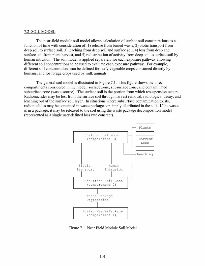
101

7.2 SOIL MODEL The near-field module soil model allows calculation of surface soil concentrations as a function of time with consideration of: 1) release from buried waste, 2) biotic transport from deep soil to surface soil, 3) leaching from deep soil and surface soil, 4) loss from deep and surface soil from plant harvest, and 5) redistribution of activity from deep soil to surface soil by human intrusion. The soil model is applied separately for each exposure pathway allowing different soil concentrations to be used to evaluate each exposure pathway. For example, different soil concentrations can be defined for leafy vegetable crops consumed directly by humans, and for forage crops used by milk animals. The general soil model is illustrated in Figure 7.1. This figure shows the three compartments considered in the model: surface zone, subsurface zone, and contaminated subsurface zone (waste source). The surface soil is the portion from which resuspension occurs. Radionuclides may be lost from the surface soil through harvest removal, radiological decay, and leaching out of the surface soil layer. In situations where subsurface contamination exists, radionuclides may be contained in waste packages or simply distributed in the soil. If the waste is in a package, it may be released to the soil using the waste package decomposition model (represented as a single user-defined loss rate constant). ┌────────┐ ┌─┤ Plants │ ┌──────────────────────────┐ │ └───┬────┘ │ Surface Soil Zone ├─┤ ┌───┴────┐ │ (compartment 3) │ │ │ Harvest│ └───┬──────────────┬─────┬─┘ │ │ Loss │ │ │ │ │ └────────┘ │ │ │ │ ┌────────┐ │ │ └─────┤Leaching│ │ │ │ └────────┘ │ │ │ Biotic Human │ Transport Intrusion │ │ │ │ ┌───┴──────────────┴───────┐ │ │ Subsurface Soil Zone ├─┘ │ (compartment 2) │ └───────────┬──────────────┘ │ Waste Package Degradation │ ┌───────────┴──────────────┐ │ Buried Waste/Package │ │ (compartment 1) │ └──────────────────────────┘

Figure 7.1 Near Field Module Soil Model

102

Radionuclides in the available subsurface soil (those not in packages) may be transported to the surface soils by root uptake by plants, by physical transport by native animals, or by human interactions through intrusion into the waste that results in redistribution of waste from deep to surface soil. Note that the model does not include transfer from the surface zone to either of the other two zones. All losses from the surface zone (harvest removal or leaching) are assumed to leave the system. The soil model allows evaluation of the soil concentration (surface soil and subsurface soil) at the start of the intake period, accounting for prior transfer from the waste package. When the source includes a waste package, the time of placement represents the start of the calculation, with the time to the start of the intake period being greater than or equal to zero. Also, the time of loss of institutional control (prior to the start of intake) is given. The soil model then evaluates the soil and waste package concentration at the start of the intake period. After the start of intake, the soil model is used to follow the change in soil compartment concentrations as intake is evaluated. The models and sub-models defined in the following section are applied on an annual basis as indicated by the time period parameter, Tyr, representing a one-year time period. Application of the soil model for agricultural pathways involves defining the fraction of roots that are in each of the soil zones. Although the model explicitly considers three compartments, the fourth is conceptually an uncontaminated layer in between the surface and deep soils. Although neglected in the model, the existence of such a layer may be simulated by appropriate application of the rooting depth fractions (see Section 7.4.1). A fraction of plant roots may be described as located in the surface soil layer, and another fraction as located in the deep soil. These two fractions may add to less than one if a clean soil layer intervenes. The model is defined by differential equations that describe the change of concentration in each compartment as a function of time. The three compartments are ordered according to transfers from one to the next. The first compartment in the model is the subsurface waste package compartment because it has no input from other compartments. The second is the subsurface soil zone because it has input from only the subsurface waste package compartment. The third is the surface soil zone because it has input from the other two compartments. This numbering is used in the nomenclature of the equations to follow. The total amount of a radionuclide in the subsurface waste package zone is decreased by radioactive decay and by loss to the subsurface soil zone. Material may also be redistributed to the surface soil zone; however, this redistribution is represented as a step function applied at the start of the analysis (representing a human action). The redistribution results in an increased initial amount of the radionuclide in the surface soil zone. The differential equations for the three soil model compartments are defined in terms of the amount of each radionuclide chain member present in units of atoms. This representation is used for ease of understanding and ease of solving the equations. The final solutions are evaluated using the radioactive decay-chain processor described in Appendix C. The general solutions presented in that appendix are given in terms of atom units and activity units. The differential equation for the subsurface contaminated zone (waste package) is as follows:

103

where A1i(t) = amount of radionuclide i in the subsurface waste package zone at time, t (atoms)

Rpi = release rate constant for release of radionuclide i from the waste package (y-1) i = radioactive decay rate constant for radionuclide i (y-1). The amount of a radionuclide in the subsurface soil zone is increased by the transfer of activity from the subsurface waste package zone, and by loss from radioactive decay and from transfer by biotic processes (plant and animal) to the surface soil zone. The differential equation for the subsurface soil zone is as follows:

where A2i(t) = amount of radionuclide i in the subsurface soil zone at time, t (atoms) Rbi = rate constant for transfer of radionuclide i from the subsurface soil zone to the

surface soil zone by biotic plant transport (y-1) Rai = rate constant for transfer of radionuclide i from the subsurface soil zone to the

surface soil zone by biotic animal transport (y-1) and other terms are as previously defined. The amount of radionuclide in the surface soil zone is increased by biotic transfer from the subsurface soil zone, and is decreased by losses from radioactive decay, leaching, and harvest. The decrease from harvest is modeled as a step function following the time of harvest and does not appear in the differential equation for the surface zone. The differential equation for the surface soil zone is as follows:

where A3i(t) = amount of radionuclide i in the surface soil zone at time, t (atoms) Li = rate constant for leaching of radionuclide from the surface soil zone (y-1) and other terms are as previously defined. Application of the soil model requires that the initial amount of each radionuclide in each compartment be known. The agricultural exposure pathway models are generally expressed per

(t)A ) + R( - = td

(t)A di1ii p

i1 (7.1)

(t)A ) + R + R( - (t)A R = td

(t)A di2ii ai bi1i p

i2 (7.2)

A ) + ( - (t)A )R + R( = td

(t)A di3iLii2i ai b

i3 (7.3)

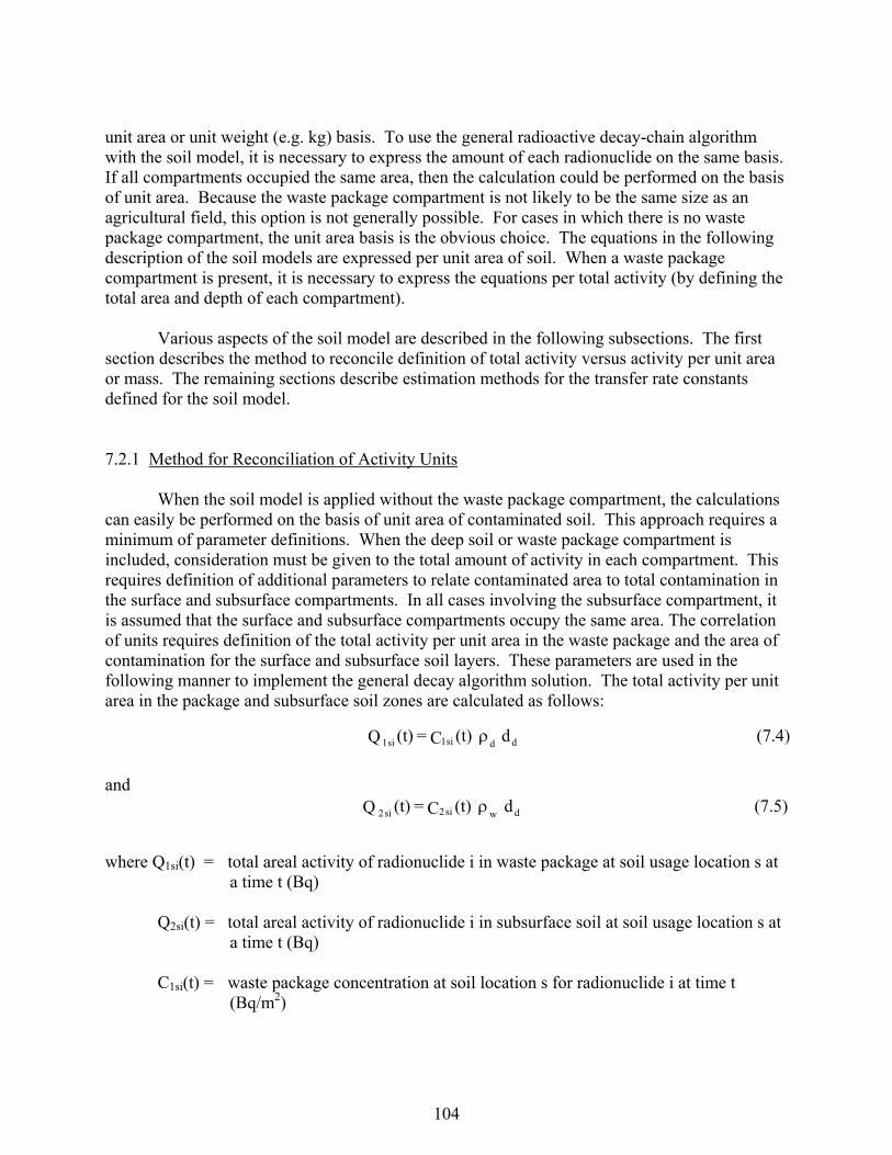
104

unit area or unit weight (e.g. kg) basis. To use the general radioactive decay-chain algorithm with the soil model, it is necessary to express the amount of each radionuclide on the same basis. If all compartments occupied the same area, then the calculation could be performed on the basis of unit area. Because the waste package compartment is not likely to be the same size as an agricultural field, this option is not generally possible. For cases in which there is no waste package compartment, the unit area basis is the obvious choice. The equations in the following description of the soil models are expressed per unit area of soil. When a waste package compartment is present, it is necessary to express the equations per total activity (by defining the total area and depth of each compartment). Various aspects of the soil model are described in the following subsections. The first section describes the method to reconcile definition of total activity versus activity per unit area or mass. The remaining sections describe estimation methods for the transfer rate constants defined for the soil model. 7.2.1 Method for Reconciliation of Activity Units When the soil model is applied without the waste package compartment, the calculations can easily be performed on the basis of unit area of contaminated soil. This approach requires a minimum of parameter definitions. When the deep soil or waste package compartment is included, consideration must be given to the total amount of activity in each compartment. This requires definition of additional parameters to relate contaminated area to total contamination in the surface and subsurface compartments. In all cases involving the subsurface compartment, it is assumed that the surface and subsurface compartments occupy the same area. The correlation of units requires definition of the total activity per unit area in the waste package and the area of contamination for the surface and subsurface soil layers. These parameters are used in the following manner to implement the general decay algorithm solution. The total activity per unit area in the package and subsurface soil zones are calculated as follows:

and

dwsi2si2 d (t)C = (t)Q (7.5)

where Q1si(t) = total areal activity of radionuclide i in waste package at soil usage location s at

a time t (Bq) Q2si(t) = total areal activity of radionuclide i in subsurface soil at soil usage location s at

a time t (Bq) C1si(t) = waste package concentration at soil location s for radionuclide i at time t

(Bq/m2)

ddsi1si1 d (t)C = (t)Q (7.4)

105

C2si(t) = subsurface soil concentration at soil location s for radionuclide i at time t (Bq/m2)

d = density of subsurface soil (kg/m3) w = density of waste package (kg/m3) dd = thickness of deep soil/waste package layer (m). The total activity in the waste package compartment for radionuclide i and soil usage location s is expressed by the parameter, Q1si(t). When the waste package compartment is included, the soil model is evaluated using the general solution algorithm with activity expressed as the total amount per unit area in each compartment (Q1si, Q2si, and Q3si). The result of the evaluation for the surface compartment is then converted back to units of activity per unit area or mass for use in the terrestrial pathway equations. 7.2.2 Release Rate from Subsurface Waste Package The rate of release of activity from the subsurface waste package is provided by the user. A rate constant is required for release directly to the subsurface soil layer (Rwpi). 7.2.3 Biotic Transfer to the Surface by Plants Plants whose roots penetrate contaminated soil layers may transport activity to the surface (McKenzie et al. 1985). This activity becomes part of the surface soil over a period of time. The rate of transfer to the surface is estimated as follows:

where Rpi = rate constant for transfer of radionuclide i from the subsurface soil zone to the surface soil zone by plant transport (y-1)

Np = number of plant species considered to contribute to plant transport. In GENII-V2,

a single composite plant type is used for computational convenience. Bvli= soil-to-plant concentration ratio for plant species l and radionuclide i (Bq/g dry

plant per Bq/g dry soil) RPdl= fraction of plant l roots in the subsurface (deep) soil zone (dimensionless). Bl = total biomass production of plant l for a year (kg/m2/y)

dd

ldlvliN

1=li p

d

B RP B = Rp

(7.6)

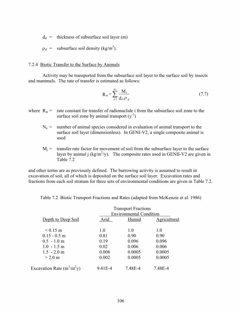
106

dd = thickness of subsurface soil layer (m) d = subsurface soil density (kg/m3). 7.2.4 Biotic Transfer to the Surface by Animals Activity may be transported from the subsurface soil layer to the surface soil by insects and mammals. The rate of transfer is estimated as follows:

where Rai = rate constant for transfer of radionuclide i from the subsurface soil zone to the surface soil zone by animal transport (y-1)

Na = number of animal species considered in evaluation of animal transport to the

surface soil layer (dimensionless). In GENI-V2, a single composite animal is used

Mj = transfer rate factor for movement of soil from the subsurface layer to the surface

layer by animal j (kg/m2/y). The composite rates used in GENII-V2 are given in Table 7.2

and other terms are as previously defined. The burrowing activity is assumed to result in excavation of soil, all of which is deposited on the surface soil layer. Excavation rates and fractions from each soil stratum for three sets of environmental conditions are given in Table 7.2. Table 7.2 Biotic Transport Fractions and Rates (adapted from McKenzie et al. 1986) Transport Fractions Environmental Condition Depth to Deep Soil Arid Humid Agricultural < 0.15 m 1.0 1.0 1.0 0.15 - 0.5 m 0.81 0.90 0.90 0.5 - 1.0 m 0.19 0.096 0.096 1.0 - 1.5 m 0.02 0.006 0.006 1.5 - 2.0 m 0.008 0.0005 0.0005 > 2.0 m 0.002 0.0005 0.0005 Excavation Rate (m3/m2y) 9.41E-4 7.48E-4 7.48E-4

d d

jN

1j=ai

d

M = Ra

(7.7)

107

7.2.5 Leaching from the Surface Soil Zone Removal from the surface soils through leaching into deeper soils is treated by means of a soil removal rate constant. For surface soils the rate constant, si, is a correction for long-term leaching of deposited radionuclides out of the surface soil (rooting and resuspension zones). The values for si are calculated using the formula of Baes and Sharp (1981):

where si = removal rate constant for activity of radionuclide i in the surface soil layer (y-1) P = total annual precipitation (cm/y) I = total irrigation rate (cm/y) E = total evapotranspiration rate (cm/y) s = surface soil bulk density (kg/m3) s = surface soil volumetric water content (mL/cm3) Kdsi = surface soil distribution coefficient for radionuclide i (mL/g) 10-2 = units conversion factor (m/cm) 103 = units conversion factor (g/kg) 10-6 = units conversion factor (m3/ml) ds = depth of surface layer (cm) 7.2.6 Loss by Harvest Loss of activity from the surface soil zone is modeled as a step function applied at the end of each calculational year. The amount of loss is calculated from the plant concentration at harvest, the annual plant yield, and the root penetration factors and the soil concentrations at harvest. The calculation is represented by the following equation.

where C3si(t+)=surface soil concentration at soil location s for radionuclide i after correction for harvest removal at time t (Bq/m2)

Kd

10 10 + 1 d

E) - I + (P 10 =

sis

s6-3

ss

-2

si

(7.8)

si3

dc-si2sc-si3

sc-si3c ci c si3-si3+si3 C/

RP )t(C + RP )t(C

RP )t(C Y )Th(CC )t(C = )t(C (7.9)

108

C 3si(t-) = surface soil concentration at soil location s for radionuclide i before correction for harvest removal at time t (Bq/m2)

Cci(Thc) = crop c concentration for radionuclide i at time of harvest (Bq/kg) C2si(t-) = subsurface soil concentration at soil location s for radionuclide i before correction

for harvest removal at time t (Bq/m2) Yc = annual yield of crop c (kg/m2) RPsc = fraction of crop c roots in the surface soil zone (dimensionless) RPdc = fraction of crop c roots in the subsurface (deep) soil zone (dimensionless). The multiplicative term represents the average fraction of the contaminant in soil to that in crops over the year; this term is used rather than a simple subtraction of amount harvested because, for short-lived radionuclides, the amount harvested over the year may actually be larger than the amount remaining in the soil at the end of the year. 7.2.7 Transfer by Redistribution Activity in the subsurface waste package may be manually redistributed to the surface soil zone by application of a redistribution factor at the start of the analysis. The redistribution is intended to represent human disruption of a site. The manual redistribution factor relates the resultant surface soil concentration, in Bq/kg, to the initial subsurface concentration, in Bq/kg. Because the surface soil is modeled as a slab 15 cm thick, a scenario in which deep soils are brought up and overlay the previous surface would use a manual redistribution factor of 1.0. If the resulting surface contamination was a mix of 75% clean soil and 25% contaminated soil, the manual redistribution factor would be 0.25. Scenarios that result in proportionately more or less redistribution would be simple multiples. 7.2.8 Soil Model Application to Near-Field Exposure Module The near-field component is designed to evaluate scenarios beginning with initial contamination of the soil. In this model the initial contamination may be in the surface soil layer, deep soil (subsurface) layer, or subsurface waste source package. The initial conditions for the near-field soil model involve definition of the activity of each radionuclide in the three zones. The initial activity is defined using a source definition module that allows the user to define the soil or waste package concentration and the volume (length, width, and depth) of each of the soil model compartments. The soil model provides estimates of soil concentration as a function of time for evaluation of media concentrations for each exposure pathway. The estimation of exposure pathway media concentrations is described in the following sections.

109

7.3 EXTERNAL EXPOSURE PATHWAYS External exposure pathways associated with the near-field component include immersion in air contaminated by resuspension, and standing on the contaminated ground. The ground external dose pathway includes modification of dose rate to account for a small area of contamination. 7.3.1 External Air Immersion This pathway is similar to the chronic pathway for immersion in a contaminated plume (Sections 5.4 or 9.3.1). The air concentration is related directly to the soil concentration by resuspension of soil particles. The air concentration used to evaluate the immersion dose is assumed to be proportional to the time-integral of soil concentration. The time-integral of the surface soil concentration for a one-year period is evaluated using Equation (7.3). The equation specific to the near-field analysis can be written as follows.

where Cesi(Tyr) = time-average of surface soil concentration for radionuclide i (Bq/m2)

C3si(Tyr) = average surface soil concentration during the current year from material present in the surface soil zone at the start of the year (Bq/m2)

Rbit = biotic transport rate from deep soil to surface soil (Bq/m2·y-1) Tyr = one year period of exposure (y).

The average surface soil concentration is evaluated using the initial concentration with decay and loss processes followed during the year. The biotic transport rate is evaluated from the biotic transport rate constants and the average activity in the subsurface soil zone over the current year, as follows.

where C2si(Tyr) = subsurface soil concentration for radionuclide i as a function of time (Bq/m2) Rbi = rate constant for transfer of activity from subsurface soil to surface soil for

plant species (y-1) Rai = rate constant for transfer of activity from subsurface soil to surface soil for

animal species (y-1)

I

T ( -

yryrLii

bityrsi3yresi

e - 1 - T T )(

R + )T(C = )T(C

yr))Lii

(7.10)

dt (t)C T

R + R = R si2

T

0yr

aibibit

yr

(7.11)

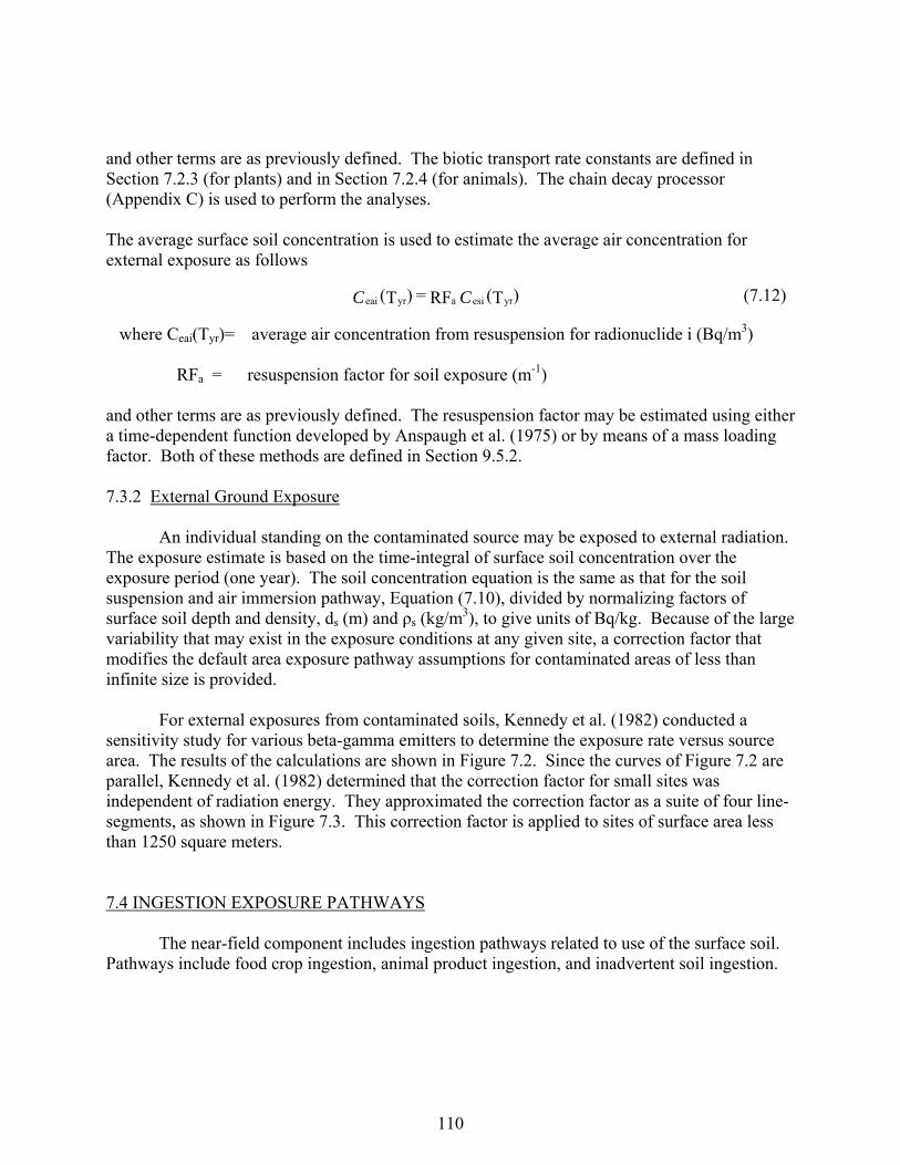
110

and other terms are as previously defined. The biotic transport rate constants are defined in Section 7.2.3 (for plants) and in Section 7.2.4 (for animals). The chain decay processor (Appendix C) is used to perform the analyses. The average surface soil concentration is used to estimate the average air concentration for external exposure as follows

where Ceai(Tyr)= average air concentration from resuspension for radionuclide i (Bq/m3) RFa = resuspension factor for soil exposure (m-1) and other terms are as previously defined. The resuspension factor may be estimated using either a time-dependent function developed by Anspaugh et al. (1975) or by means of a mass loading factor. Both of these methods are defined in Section 9.5.2. 7.3.2 External Ground Exposure An individual standing on the contaminated source may be exposed to external radiation. The exposure estimate is based on the time-integral of surface soil concentration over the exposure period (one year). The soil concentration equation is the same as that for the soil suspension and air immersion pathway, Equation (7.10), divided by normalizing factors of surface soil depth and density, ds (m) and ρs (kg/m3), to give units of Bq/kg. Because of the large variability that may exist in the exposure conditions at any given site, a correction factor that modifies the default area exposure pathway assumptions for contaminated areas of less than infinite size is provided. For external exposures from contaminated soils, Kennedy et al. (1982) conducted a sensitivity study for various beta-gamma emitters to determine the exposure rate versus source area. The results of the calculations are shown in Figure 7.2. Since the curves of Figure 7.2 are parallel, Kennedy et al. (1982) determined that the correction factor for small sites was independent of radiation energy. They approximated the correction factor as a suite of four line-segments, as shown in Figure 7.3. This correction factor is applied to sites of surface area less than 1250 square meters. 7.4 INGESTION EXPOSURE PATHWAYS The near-field component includes ingestion pathways related to use of the surface soil. Pathways include food crop ingestion, animal product ingestion, and inadvertent soil ingestion.

)T( RF = )T( yresiayreai CC (7.12)

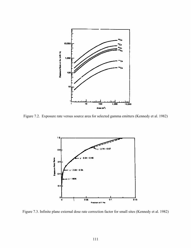
111

Figure 7.2. Exposure rate versus source area for selected gamma emitters (Kennedy et al. 1982)

Figure 7.3. Infinite plane external dose rate correction factor for small sites (Kennedy et al. 1982)

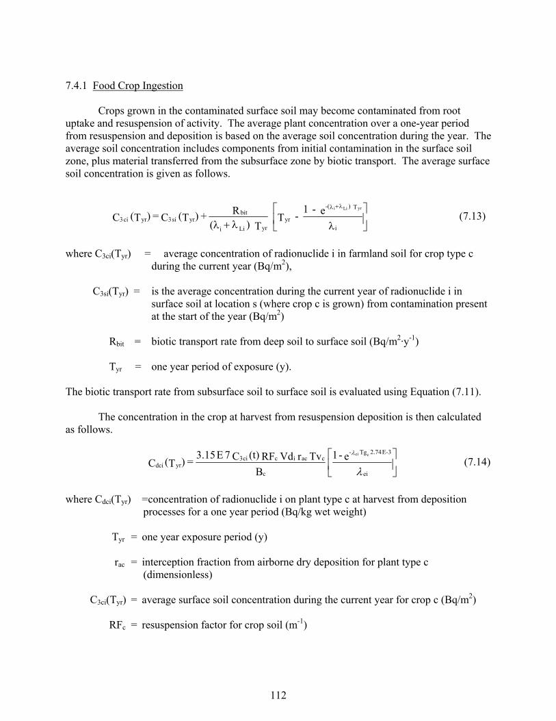
112

7.4.1 Food Crop Ingestion Crops grown in the contaminated surface soil may become contaminated from root uptake and resuspension of activity. The average plant concentration over a one-year period from resuspension and deposition is based on the average soil concentration during the year. The average soil concentration includes components from initial contamination in the surface soil zone, plus material transferred from the subsurface zone by biotic transport. The average surface soil concentration is given as follows.

where C3ci(Tyr) = average concentration of radionuclide i in farmland soil for crop type c during the current year (Bq/m2),

C3si(Tyr) = is the average concentration during the current year of radionuclide i in

surface soil at location s (where crop c is grown) from contamination present at the start of the year (Bq/m2)

Rbit = biotic transport rate from deep soil to surface soil (Bq/m2·y-1) Tyr = one year period of exposure (y). The biotic transport rate from subsurface soil to surface soil is evaluated using Equation (7.11). The concentration in the crop at harvest from resuspension deposition is then calculated as follows.

where Cdci(Tyr) =concentration of radionuclide i on plant type c at harvest from deposition processes for a one year period (Bq/kg wet weight)

Tyr = one year exposure period (y) rac = interception fraction from airborne dry deposition for plant type c

(dimensionless) C3ci(Tyr) = average surface soil concentration during the current year for crop c (Bq/m2) RFc = resuspension factor for crop soil (m-1)

i

T )-(

yryrLii

bityrsi3yrci3

e - 1 - T

T )(R + )T( C = )T( C

yrLii

(7.13)

ei

3E-2.74 Tg -

c

cacicci3yrdci

e - 1 B

Tv r Vd RF (t)C 7E3.15 = )T(C

cei

(7.14)

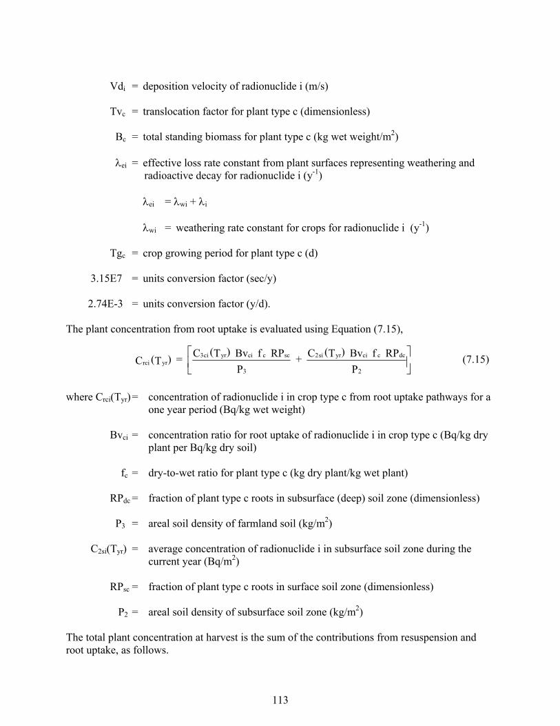
113

Vdi = deposition velocity of radionuclide i (m/s) Tvc = translocation factor for plant type c (dimensionless) Bc = total standing biomass for plant type c (kg wet weight/m2) ei = effective loss rate constant from plant surfaces representing weathering and

radioactive decay for radionuclide i (y-1) ei = wi + i wi = weathering rate constant for crops for radionuclide i (y-1) Tgc = crop growing period for plant type c (d) 3.15E7 = units conversion factor (sec/y) 2.74E-3 = units conversion factor (y/d). The plant concentration from root uptake is evaluated using Equation (7.15),

where Crci(Tyr) = concentration of radionuclide i in crop type c from root uptake pathways for a one year period (Bq/kg wet weight)

Bvci = concentration ratio for root uptake of radionuclide i in crop type c (Bq/kg dry

plant per Bq/kg dry soil) fc = dry-to-wet ratio for plant type c (kg dry plant/kg wet plant) RPdc = fraction of plant type c roots in subsurface (deep) soil zone (dimensionless) P3 = areal soil density of farmland soil (kg/m2) C2si(Tyr) = average concentration of radionuclide i in subsurface soil zone during the

current year (Bq/m2) RPsc = fraction of plant type c roots in surface soil zone (dimensionless) P2 = areal soil density of subsurface soil zone (kg/m2) The total plant concentration at harvest is the sum of the contributions from resuspension and root uptake, as follows.

P

RP f Bv )T(C +

P

RP f Bv )T(C = )T(C

2

dccciyrsi2

3

sccciyrci3yrrci (7.15)

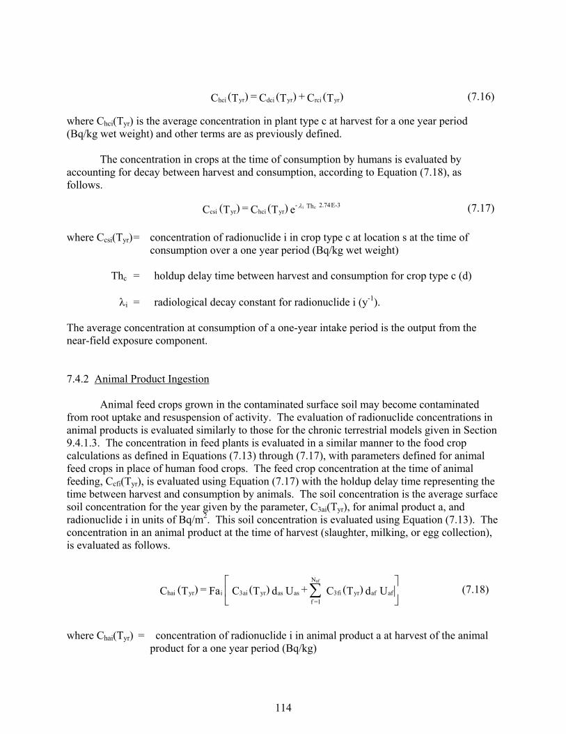
114

where Chci(Tyr) is the average concentration in plant type c at harvest for a one year period (Bq/kg wet weight) and other terms are as previously defined. The concentration in crops at the time of consumption by humans is evaluated by accounting for decay between harvest and consumption, according to Equation (7.18), as follows.

where Ccsi(Tyr) = concentration of radionuclide i in crop type c at location s at the time of consumption over a one year period (Bq/kg wet weight)

Thc = holdup delay time between harvest and consumption for crop type c (d) i = radiological decay constant for radionuclide i (y-1). The average concentration at consumption of a one-year intake period is the output from the near-field exposure component. 7.4.2 Animal Product Ingestion Animal feed crops grown in the contaminated surface soil may become contaminated from root uptake and resuspension of activity. The evaluation of radionuclide concentrations in animal products is evaluated similarly to those for the chronic terrestrial models given in Section 9.4.1.3. The concentration in feed plants is evaluated in a similar manner to the food crop calculations as defined in Equations (7.13) through (7.17), with parameters defined for animal feed crops in place of human food crops. The feed crop concentration at the time of animal feeding, Ccfi(Tyr), is evaluated using Equation (7.17) with the holdup delay time representing the time between harvest and consumption by animals. The soil concentration is the average surface soil concentration for the year given by the parameter, C3ai(Tyr), for animal product a, and radionuclide i in units of Bq/m2. This soil concentration is evaluated using Equation (7.13). The concentration in an animal product at the time of harvest (slaughter, milking, or egg collection), is evaluated as follows.

where Chai(Tyr) = concentration of radionuclide i in animal product a at harvest of the animal product for a one year period (Bq/kg)

)T(C + )T(C = )T(C yrrciyrdciyrhci (7.16)

e )T(C = )T( C 3E-2.74 Th -yrhciyrcsi

ci (7.17)

U d )T(C +U d )T(C Fa = )T( C afafyrfi3

N

1=fasasyrai3iyrhai

af

(7.18)

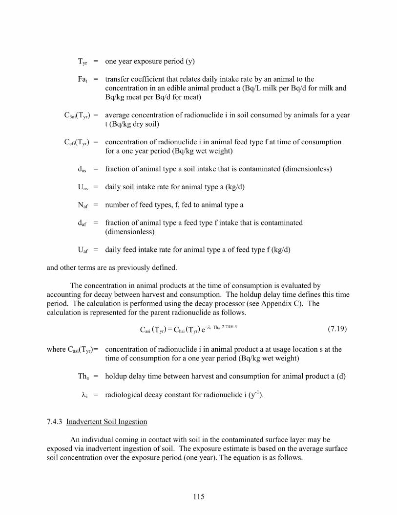
115

Tyr = one year exposure period (y) Fai = transfer coefficient that relates daily intake rate by an animal to the

concentration in an edible animal product a (Bq/L milk per Bq/d for milk and Bq/kg meat per Bq/d for meat)

C3ai(Tyr) = average concentration of radionuclide i in soil consumed by animals for a year

t (Bq/kg dry soil) Ccfi(Tyr) = concentration of radionuclide i in animal feed type f at time of consumption

for a one year period (Bq/kg wet weight) das = fraction of animal type a soil intake that is contaminated (dimensionless) Uas = daily soil intake rate for animal type a (kg/d) Naf = number of feed types, f, fed to animal type a daf = fraction of animal type a feed type f intake that is contaminated

(dimensionless) Uaf = daily feed intake rate for animal type a of feed type f (kg/d) and other terms are as previously defined. The concentration in animal products at the time of consumption is evaluated by accounting for decay between harvest and consumption. The holdup delay time defines this time period. The calculation is performed using the decay processor (see Appendix C). The calculation is represented for the parent radionuclide as follows.

where Casi(Tyr) = concentration of radionuclide i in animal product a at usage location s at the time of consumption for a one year period (Bq/kg wet weight)

Tha = holdup delay time between harvest and consumption for animal product a (d) i = radiological decay constant for radionuclide i (y-1). 7.4.3 Inadvertent Soil Ingestion An individual coming in contact with soil in the contaminated surface layer may be exposed via inadvertent ingestion of soil. The exposure estimate is based on the average surface soil concentration over the exposure period (one year). The equation is as follows.

e )T(C = )T( C 3E-2.74 Th -yrhaiyrasi

ai (7.19)

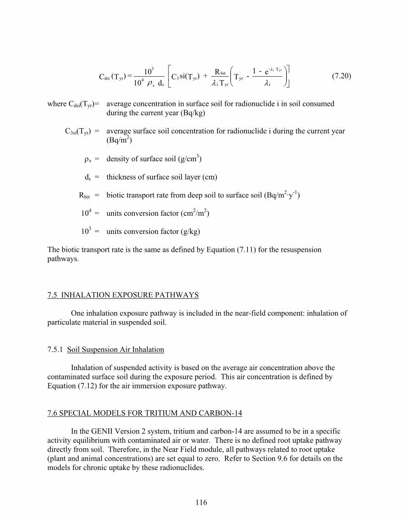
116

where Cdsi(Tyr) = average concentration in surface soil for radionuclide i in soil consumed during the current year (Bq/kg)

C3si(Tyr) = average surface soil concentration for radionuclide i during the current year

(Bq/m2) s = density of surface soil (g/cm3) ds = thickness of surface soil layer (cm) Rbit = biotic transport rate from deep soil to surface soil (Bq/m2·y-1) 104 = units conversion factor (cm2/m2) 103 = units conversion factor (g/kg) The biotic transport rate is the same as defined by Equation (7.11) for the resuspension pathways. 7.5 INHALATION EXPOSURE PATHWAYS One inhalation exposure pathway is included in the near-field component: inhalation of particulate material in suspended soil. 7.5.1 Soil Suspension Air Inhalation Inhalation of suspended activity is based on the average air concentration above the contaminated surface soil during the exposure period. This air concentration is defined by Equation (7.12) for the air immersion exposure pathway. 7.6 SPECIAL MODELS FOR TRITIUM AND CARBON-14 In the GENII Version 2 system, tritium and carbon-14 are assumed to be in a specific activity equilibrium with contaminated air or water. There is no defined root uptake pathway directly from soil. Therefore, in the Near Field module, all pathways related to root uptake (plant and animal concentrations) are set equal to zero. Refer to Section 9.6 for details on the models for chronic uptake by these radionuclides.

i

T -

yryri

bityr3

ss4

3

yrdsie - 1

- TT

R + )Tsi(C d 10

10 = )T( Cyri

(7.20)

117

7.7 REFERENCES FOR SECTION 7 Anspaugh, L. R., J. H. Shinn, P. L. Phelps, and N. C. Kennedy. 1975. "Resuspension and Redistribution of Plutonium in Soils." Health Phys. 29:571-582. Baes, C. F., and R. D. Sharp. 1981. Predicting Radionuclide Leaching From Root Zone Soil From Assessment Applications. CONF-81606, Oak Ridge National Laboratory, Oak Ridge, Tennessee. Kennedy, W.E., R.A. Peloquin, B.A. Napier, and S.M. Neuder. 1982. Intruder Dose Pathway Analysis for the Onsite Disposal of Radioactive Wastes: The ONSITE/MAXI1 Computer Program, NUREG/CR-3620, Pacific Northwest Laboratory, Richland, Washington. McKenzie, D. H., L. L. Cadwell, K. A. Gano, W. E. Kennedy, Jr., B. A. Napier, R. A. Peloquin, L. A. Prohammer, and M. A. Simmons. 1986. Relevance of Biotic Pathways to the Long-term Regulation of Nuclear waste Disposal: Estimation of Radiation Dose to Man Resulting form Biotic Transport: The BIOPORT/MAXI1 Software Package. NUREG/ CR-2675, Vol. 5, prepared for U.S. Nuclear Regulatory Commission by Pacific Northwest Laboratory, Richland, Washington.

118

8.0 ACUTE EXPOSURE MODULE

The acute exposure module provides estimates of exposure media concentration for short-term contamination of air or surface water. The models are defined to represent situations in which the release or exposure occurs over a relatively short period of time. Acute releases are typically on the order of a few hours or less, with exposures occurring over a period from a few hours (e.g., for air transport) to a few months (e.g., deposition onto soil with subsequent external or crop ingestion exposure). Exposure from residual contamination in soil could also occur over a many-year period and is included in the analysis. The module includes models to represent the amount of activity in soil as a function of time and exposure pathway models for specific exposure routes (external, ingestion, and inhalation).

The acute exposure module estimates exposure media concentrations for the exposure pathways listed in Table 8.1. As indicated in the table, some exposure pathways are not evaluated for the acute exposure period, but only for exposure to residual contamination during the long-term period immediately following the acute period. Model details are given in the following sections. Table 8.1 Exposure Pathways for the Acute Exposure Module Transport Mode Exposure Pathways Exposure Period atmospheric air inhalation acute/chronic soil resuspension chronic soil ingestion chronic air external acute/chronic ground exposure chronic food crops chronic animal products chronic surface water drinking water ingestion acute/chronic shower volatilization acute/chronic shower water ingestion acute/chronic irrigated food crops chronic irrigation/animal products chronic ground exposure chronic swimming ingestion acute/chronic swimming external acute/chronic swimming water ingestion acute/chronic boating external acute/chronic shoreline sediment ingestion chronic shoreline external chronic aquatic foods chronic soil contamination soil resuspension chronic soil ingestion chronic ground exposure chronic

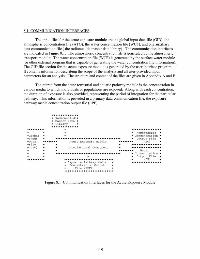
119

8.1 COMMUNICATION INTERFACES The input files for the acute exposure module are the global input data file (GID), the atmospheric concentration file (ATO), the water concentration file (WCF), and one auxiliary data communication file ( the radionuclide master data library). The communication interfaces are indicated in Figure 8.1. The atmospheric concentration file is generated by the atmospheric transport module. The water concentration file (WCF) is generated by the surface water module (or other external program that is capable of generating the water concentration file information). The GID file section for the acute exposure module is generated by the user interface program. It contains information describing the scope of the analysis and all user-provided input parameters for an analysis. The structure and content of the files are given in Appendix A and B. The output from the acute terrestrial and aquatic pathway module is the concentration in various media to which individuals or populations are exposed. Along with each concentration, the duration of exposure is also provided, representing the period of integration for the particular pathway. This information is provided in a primary data communication file, the exposure pathway media concentration output file (EPF). ••••••••••••••• • Radionuclide• • Master Data • • Library • ••••••••••••••• •••••••••• • ••••••••••••••••• • • • • Atmospheric • •Global • • • Concentration • •Input • ••••••••••••••••••••••••••••••••••••• • Output File • •Data •••••••• Acute Exposure Module •••••••• (ATO) • •File • • • ••••••••••••••••• •(GID) • • Calculational Component • ••••••••••••••••• • • • •••••••• Water • • • ••••••••••••••••••••••••••••••••••••• • Concentration • • • • • Output File • •••••••••• •••••••••••••••••••••••••••• • (WCF) • • Exposure Pathway Media • ••••••••••••••••• • Concentration Output • • File (EPF) • ••••••••••••••••••••••••••••

Figure 8.1 Communication Interfaces for the Acute Exposure Module

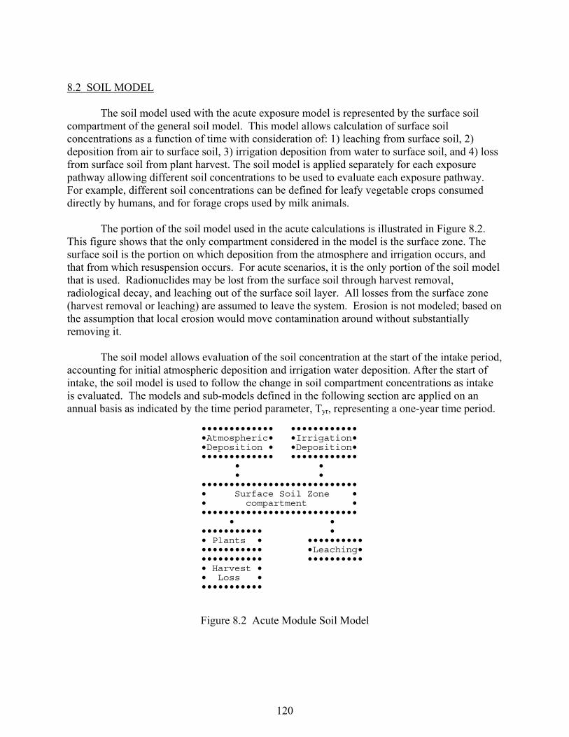
120

8.2 SOIL MODEL The soil model used with the acute exposure model is represented by the surface soil compartment of the general soil model. This model allows calculation of surface soil concentrations as a function of time with consideration of: 1) leaching from surface soil, 2) deposition from air to surface soil, 3) irrigation deposition from water to surface soil, and 4) loss from surface soil from plant harvest. The soil model is applied separately for each exposure pathway allowing different soil concentrations to be used to evaluate each exposure pathway. For example, different soil concentrations can be defined for leafy vegetable crops consumed directly by humans, and for forage crops used by milk animals. The portion of the soil model used in the acute calculations is illustrated in Figure 8.2. This figure shows that the only compartment considered in the model is the surface zone. The surface soil is the portion on which deposition from the atmosphere and irrigation occurs, and that from which resuspension occurs. For acute scenarios, it is the only portion of the soil model that is used. Radionuclides may be lost from the surface soil through harvest removal, radiological decay, and leaching out of the surface soil layer. All losses from the surface zone (harvest removal or leaching) are assumed to leave the system. Erosion is not modeled; based on the assumption that local erosion would move contamination around without substantially removing it. The soil model allows evaluation of the soil concentration at the start of the intake period, accounting for initial atmospheric deposition and irrigation water deposition. After the start of intake, the soil model is used to follow the change in soil compartment concentrations as intake is evaluated. The models and sub-models defined in the following section are applied on an annual basis as indicated by the time period parameter, Tyr, representing a one-year time period. ••••••••••••• •••••••••••• •Atmospheric• •Irrigation• •Deposition • •Deposition• ••••••••••••• •••••••••••• • • • • •••••••••••••••••••••••••••• • Surface Soil Zone • • compartment • •••••••••••••••••••••••••••• • • ••••••••••• • • Plants • •••••••••• ••••••••••• •Leaching• ••••••••••• •••••••••• • Harvest • • Loss • ••••••••••• Figure 8.2 Acute Module Soil Model

121

The model is defined by a differential equation that describes the change of concentration as a function of time. The decrease from harvest is modeled as a step function following the time of harvest and does not appear in the differential equation for the surface zone. The differential equation for acute releases for the surface soil zone is as follows:

where A0i = initial deposition on soil surface at time 0, (atoms) Ai(t) = amount of radionuclide i in the surface soil zone at time t (atoms) Li = rate constant for leaching of radionuclide from the surface soil zone (y-1). Various aspects of the soil model are described in the following subsections. The first section describes definition of the initial amount in the surface compartment for air and water deposition for acute releases. The remaining sections describe estimation methods for the transfer rate constants defined for the soil model. 8.2.1 Activity from Air and Water Deposition The soil model for acute releases requires an estimate of the initial activity in each compartment. The initial activity in the surface soil is related to the transport analysis for air or water. The initial soil activity can be evaluated using estimates from the atmospheric transport component deposition estimates. The deposition estimate parameter for acute releases is the amount of a radionuclide deposited at a location from wet or dry deposition (two parameter values). The deposition amounts may be summed to give the total deposition, taken to be the initial amount present at time zero (assuming a short acute release and deposition period). For deposition from surface water, the initial soil activity is given as follows.

where Csi(0) = initial aerial concentration of radionuclide i in soil at soil usage location s (Bq/m2)

Ewi = time integrated average water concentration at surface water usage location w

for radionuclide i over the time of contamination passage (Equation 6.3) (Bq/L) IRw = application rate of irrigation water at water usage location w (L/m2/sec) Tw = period over which the release of contamination to surface water passes the usage

location w (sec).

A + - = td

(t)A di0iLi

i (8.1)

T IR E = (0)C wwwisi (8.2)

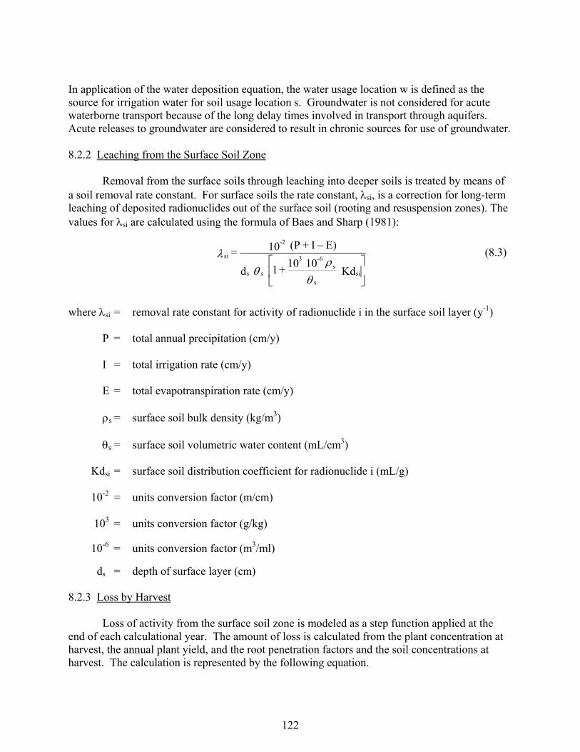
122

In application of the water deposition equation, the water usage location w is defined as the source for irrigation water for soil usage location s. Groundwater is not considered for acute waterborne transport because of the long delay times involved in transport through aquifers. Acute releases to groundwater are considered to result in chronic sources for use of groundwater. 8.2.2 Leaching from the Surface Soil Zone Removal from the surface soils through leaching into deeper soils is treated by means of a soil removal rate constant. For surface soils the rate constant, si, is a correction for long-term leaching of deposited radionuclides out of the surface soil (rooting and resuspension zones). The values for si are calculated using the formula of Baes and Sharp (1981):

where si = removal rate constant for activity of radionuclide i in the surface soil layer (y-1) P = total annual precipitation (cm/y) I = total irrigation rate (cm/y) E = total evapotranspiration rate (cm/y) s = surface soil bulk density (kg/m3) s = surface soil volumetric water content (mL/cm3) Kdsi = surface soil distribution coefficient for radionuclide i (mL/g) 10-2 = units conversion factor (m/cm) 103 = units conversion factor (g/kg) 10-6 = units conversion factor (m3/ml) ds = depth of surface layer (cm) 8.2.3 Loss by Harvest Loss of activity from the surface soil zone is modeled as a step function applied at the end of each calculational year. The amount of loss is calculated from the plant concentration at harvest, the annual plant yield, and the root penetration factors and the soil concentrations at harvest. The calculation is represented by the following equation.

Kd 10 10

+ 1 d

E) I + (P 10 =

sis

s6-3

ss

-2

si

(8.3)

123

where Csi(t+) = surface soil concentration at soil location s for radionuclide i after correction for harvest removal at time t (Bq/m2)

Csi(t-) = surface soil concentration at soil location s for radionuclide i before correction

for harvest removal at time t (Bq/m2) Chci(Thc) = crop c concentration for radionuclide i at time of harvest (Bq/kg) Yc = annual yield of crop c (kg/m2) The multiplicative term represents the average fraction of the contaminant in soil to that in crops over the year; this term is used rather than a simple subtraction of amount harvested because, for short-lived radionuclides, the amount harvested over the year may actually be larger than the amount remaining in the soil at the end of the year. 8.3 EXTERNAL EXPOSURE PATHWAYS Four exposure pathways are included for acute releases that involve external exposure from radionuclides in a contaminated medium: immersion in air, standing on ground, swimming or boating in water, and standing on shoreline. 8.3.1 External Plume Immersion Two models are available for estimation of the dose from exposure to external radiation from an airborne plume of radioactivity. The simpler model is based on the assumption that the plume is essentially infinite in size, bounded by the ground plane. This model is referred to as the semi-infinite plume model. The second model is referred to as the finite plume model because it considers the finite dimensions of the plume in evaluation of the dose at the ground-level receptor location. The output from the semi-infinite plume model is the time-integrated air concentration at the exposure location(s) (Equations 5.20 or 5.27). The output from the finite plume model is the time-integrated radiation dose at the exposure location(s). For both models, the output file (EPF) also contains the exposure period over which the average air concentration or radiation dose apply. Also, for both models, the time-integrated radiation dose or average air concentration are provided in the atmospheric transport output file (ATO) and the only modifications to the values made in the exposure component (other than to select the values for the appropriate exposure location) are to average the time integral, as

Ceai(Tex) = Eeai / Tex. (8.5)

C/Y )Th(C - C)t(C = )t(C sic ci hc si-si+si (8.4)

124

Evaluation of dose or risk for the finite plume model is difficult because of the necessity to consider the finite dimensions of the plume. The structure of the software was designed to include the finite plume dose calculation in the atmospheric transport calculation. This structure was selected because information on the plume dimensions is not available in the exposure module. The acute atmospheric transport module performs a finite-plume dose calculation, and then generates the time-integrated radiation dose at a location in the environment. This approach requires more analysis for the atmospheric transport module (Section 5.4) but less analysis for the acute exposure analysis component. 8.3.2 External Groundshine Model Radioactivity deposited onto ground can cause exposure to individuals near the contamination. The exposure starts at the time of acute deposition and continues as long as the individual is present and the radioactivity remains in the surface soil zone. The deposition may be from either atmospheric or irrigation deposition. The output of the external exposure analysis from acute deposition is the time-integral of soil concentration over the period of exposure. This concentration is evaluated considering decay and progeny ingrowth according to the soil model (see Section 8.2). Airborne deposition is assumed to cover the entire region of the defined population group (e.g., sector segment boundary), and all individuals are potentially exposed. The deposition amount is used to evaluate population and individual exposures. For waterborne deposition, the soil contamination is assumed to expose only a few individuals (population dose is not available) because water transport pathways (e.g., irrigation) will not result in widespread contamination. The general term used for estimation of radiation dose from soil contamination is as follows:

where Cesi(Teg)= time integrated average soil concentration from deposition of activity to soil for radionuclide i (Bq/kg)

ds = thickness of soil (m) s = density of soil (kg/m3) Teg = exposure time to contaminated ground (y) Csi(t) = concentration of radionuclide i in soil at soil usage location s as a function of

time (Bq/m2). This equation is applied to airborne and waterborne deposition defined according to the initial deposition. The soil concentration time integral is evaluated using the radioactive chain-decay processor (see Appendix C).

)ρd(T/dt (t) C = )T(C ssegsi

T

0

egesi

eg

(8.6)

125

8.3.3 External Exposure from Aquatic Recreational Activities Aquatic recreational activities involving external exposure include swimming, external exposure while boating, and external exposure while on shoreline. The output parameter for these exposure pathways is the average water or shoreline sediment concentration over the period of contamination. For swimming and boating, the period of contamination is the acute release water contamination period. For the sediment pathways, the period of contamination is the first year after the initial deposition to sediment. For swimming and boating pathways, the average water concentration is evaluated from the time-integral average of water concentration Ewi given by Equation (6.3), described in Section 6.1. The water concentration is used for swimming and boating activities. For boating, the parameter is represented as Cbri(Teb), where Teb is the same as Tew (i.e., the exposure time for boating and swimming are the same). The exposure time periods are directly related to the time period of water contamination that is inherent in the evaluation of Ewi. The exposure from recreational activities on shoreline involves estimation of the radionuclide concentration in shoreline sediments. The initial deposition to sediment is estimated from a model developed by Soldat, Robinson, and Baker (1974) relating water concentration to sediment concentration following a long period of deposition. For acute release situations the sediment concentration is estimated directly from the time-integrated water concentration. The initial sediment concentration is estimated as follows.

where Csri(0) = initial concentration of radionuclide i in sediment after the acute water contamination period at location r (Bq-yr/m2)

Ewi = time integral average of water concentration during passage of contaminated

water at location r (Bq/L) TC = transfer constant from water to sediment (L/m2/y). The value of the transfer constant was derived for several radionuclides by using data obtained from analyzing water and sediment samples taken from the Columbia River between Richland, Washington, and the river mouth, and from Tillamook Bay, Oregon, 75 km south of the river mouth (Nelson 1965; Toombs and Cutler 1968). This data was analyzed by Soldat, Robinson, and Baker (1974) to derive a value of 2.54x104 in units of L/m2/y. Equation (8.7) estimates an effective surface contamination for calculating gamma exposure rates to persons standing on sediment. The average shoreline sediment concentration over the first year following deposition is the output parameter for the shoreline external dose pathway, and is evaluated as follows:

wisri ETC(0)C (8.7)

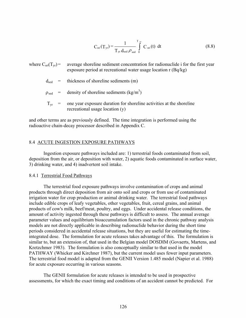
126

where Csri(Tyr) = average shoreline sediment concentration for radionuclide i for the first year exposure period at recreational water usage location r (Bq/kg)

dsed = thickness of shoreline sediments (m) sed = density of shoreline sediments (kg/m3) Tyr = one year exposure duration for shoreline activities at the shoreline

recreational usage location (y) and other terms are as previously defined. The time integration is performed using the radioactive chain-decay processor described in Appendix C. 8.4 ACUTE INGESTION EXPOSURE PATHWAYS Ingestion exposure pathways included are: 1) terrestrial foods contaminated from soil, deposition from the air, or deposition with water, 2) aquatic foods contaminated in surface water, 3) drinking water, and 4) inadvertent soil intake. 8.4.1 Terrestrial Food Pathways The terrestrial food exposure pathways involve contamination of crops and animal products through direct deposition from air onto soil and crops or from use of contaminated irrigation water for crop production or animal drinking water. The terrestrial food pathways include edible crops of leafy vegetables, other vegetables, fruit, cereal grains, and animal products of cow's milk, beef/meat, poultry, and eggs. Under accidental release conditions, the amount of activity ingested through these pathways is difficult to assess. The annual average parameter values and equilibrium bioaccumulation factors used in the chronic pathway analysis models are not directly applicable in describing radionuclide behavior during the short time periods considered in accidental release situations, but they are useful for estimating the time-integrated dose. The formulation for acute releases takes advantage of this. The formulation is similar to, but an extension of, that used in the Belgian model DOSDIM (Govaerts, Martens, and Kretzchmer 1983). The formulation is also conceptually similar to that used in the model PATHWAY (Whicker and Kirchner 1987), but the current model uses fewer input parameters. The terrestrial food model is adapted from the GENII Version 1.485 model (Napier et al. 1988) for acute exposure occurring in various seasons.

The GENII formulation for acute releases is intended to be used in prospective assessments, for which the exact timing and conditions of an accident cannot be predicted. For

dt (t)C d T

1 = )T(C sri

T

0sedsedyryrsri

yr

(8.8)

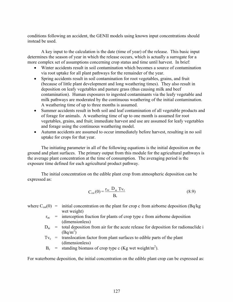
127

conditions following an accident, the GENII models using known input concentrations should instead be used. A key input to the calculation is the date (time of year) of the release. This basic input determines the season of year in which the release occurs, which is actually a surrogate for a more complex set of assumptions concerning crop status and time until harvest. In brief:

Winter accidents result in soil contamination which becomes a source of contamination via root uptake for all plant pathways for the remainder of the year.

Spring accidents result in soil contamination for root vegetables, grains, and fruit (because of little plant development and long weathering times). They also result in deposition on leafy vegetables and pasture grass (thus causing milk and beef contamination). Human exposures to ingested contaminants via the leafy vegetable and milk pathways are moderated by the continuous weathering of the initial contamination. A weathering time of up to three months is assumed.

Summer accidents result in both soil and leaf contamination of all vegetable products and of forage for animals. A weathering time of up to one month is assumed for root vegetables, grains, and fruit; immediate harvest and use are assumed for leafy vegetables and forage using the continuous weathering model.

Autumn accidents are assumed to occur immediately before harvest, resulting in no soil uptake for crops for that year.

The initiating parameter in all of the following equations is the initial deposition on the ground and plant surfaces. The primary output from this module for the agricultural pathways is the average plant concentration at the time of consumption. The averaging period is the exposure time defined for each agricultural product pathway. The initial concentration on the edible plant crop from atmospheric deposition can be expressed as:

where Ccai(0) = initial concentration on the plant for crop c from airborne deposition (Bq/kg wet weight)

rac = interception fraction for plants of crop type c from airborne deposition (dimensionless)

Dai = total deposition from air for the acute release for deposition for radionuclide i (Bq/m2)

Tvc = translocation factor from plant surfaces to edible parts of the plant (dimensionless)

Bc = standing biomass of crop type c (Kg wet weight/m2). For waterborne deposition, the initial concentration on the edible plant crop can be expressed as:

B

Tv D r = (0)Cc

caiaccai (8.9)

128

where Ccwi(0) = concentration on the plant at the time of harvest for crop c from waterborne deposition (Bq/kg wet weight)

Dwi = total deposition from water for the acute release for deposition for radionuclide i (Bq/m2)

rwc = interception fraction for plants of crop type c from waterborne deposition (dimensionless)

The initial plant concentration due to the initial deposition decreases over time by means

of radiological decay and weathering. These processes are assumed to occur continuously from deposition to harvest. The plant concentration at the time of harvest Tharv (measured from the time of deposition) is calculated as

harvwii T)(

ciharvci e)0(C)T(C (8.11)

where λwi = weathering removal rate, days-1. After harvest, a delay period usually occurs before consumption of the food product begins. During this delay, additional radiological decay may occur. No other losses (such as in food preparation) are assumed. For some crops, the consumption period may last for weeks or months. To estimate the average crop concentration, the consumption is assumed to occur at a uniform rate. The average crop concentration is evaluated as follows:

where Ccsi(Tfc) = average crop concentration at usage location s for radionuclide i and crop c over the crop intake period, Tfc (Bq/kg wet weight)

Tfc = the length of the uptake period for food crop c (d) t = delay period between harvest and the start of consumption (d) Consumption of contaminated animal products is treated in a manner similar to the food crop analysis. The animal is assumed to eat contaminated crops or drink contaminated water and produce contaminated products continuously over the consumption period defined for humans. The meat and milk animal are assumed to be fed fresh forage and stored feed, to ingest contatminated soil, and to drink contaminated water (for waterborne transport analyses). The concentration in fresh forage and stored feed at the time of harvest is evaluated using Equation 8.11, with parameters defined for the forage plant or stored feed plant. The crops are assumed to be harvested following the acute deposition and to be fed to the animals over the following

B

Tv D r = (0)Cc

ciwwccwi (8.10)

dte) T( C + )T( C T

1 = )T(C

tharvcwiharvcai

T

0fcfccsi

i

fc

(8.12)

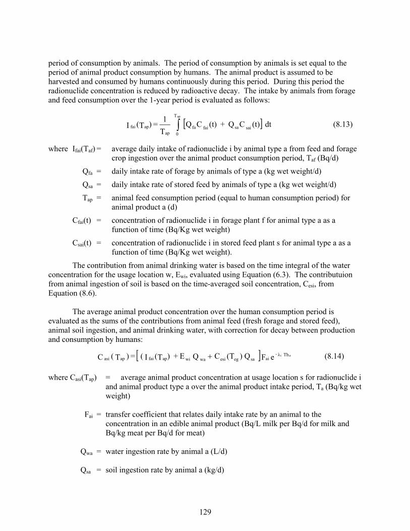
129

period of consumption by animals. The period of consumption by animals is set equal to the period of animal product consumption by humans. The animal product is assumed to be harvested and consumed by humans continuously during this period. During this period the radionuclide concentration is reduced by radioactive decay. The intake by animals from forage and feed consumption over the 1-year period is evaluated as follows:

where Ifai(Taf) = average daily intake of radionuclide i by animal type a from feed and forage crop ingestion over the animal product consumption period, Taf (Bq/d)

Qfa = daily intake rate of forage by animals of type a (kg wet weight/d)

Qsa = daily intake rate of stored feed by animals of type a (kg wet weight/d)

Tap = animal feed consumption period (equal to human consumption period) for animal product a (d)

Cfai(t) = concentration of radionuclide i in forage plant f for animal type a as a function of time (Bq/Kg wet weight)

Csai(t) = concentration of radionuclide i in stored feed plant s for animal type a as a function of time (Bq/Kg wet weight).

The contribution from animal drinking water is based on the time integral of the water concentration for the usage location w, Ewi, evaluated using Equation (6.3). The contributuion from animal ingestion of soil is based on the time-averaged soil concentration, Cesi, from Equation (8.6). The average animal product concentration over the human consumption period is evaluated as the sums of the contributions from animal feed (fresh forage and stored feed), animal soil ingestion, and animal drinking water, with correction for decay between production and consumption by humans:

where Casi(Tap) = average animal product concentration at usage location s for radionuclide i and animal product type a over the animal product intake period, Ta (Bq/kg wet weight)

Fai = transfer coefficient that relates daily intake rate by an animal to the

concentration in an edible animal product (Bq/L milk per Bq/d for milk and Bq/kg meat per Bq/d for meat)

Qwa = water ingestion rate by animal a (L/d) Qsa = soil ingestion rate by animal a (kg/d)

dt (t)CQ + (t)CQ T

1 = )T(I sa sai fa fai

T

0apapfai

ap

(8.13)

e F Q)(TCQ E + )T(I ( = ) T ( C Th λ - aisaegesi wawiapfai apasi

ai (8.14)

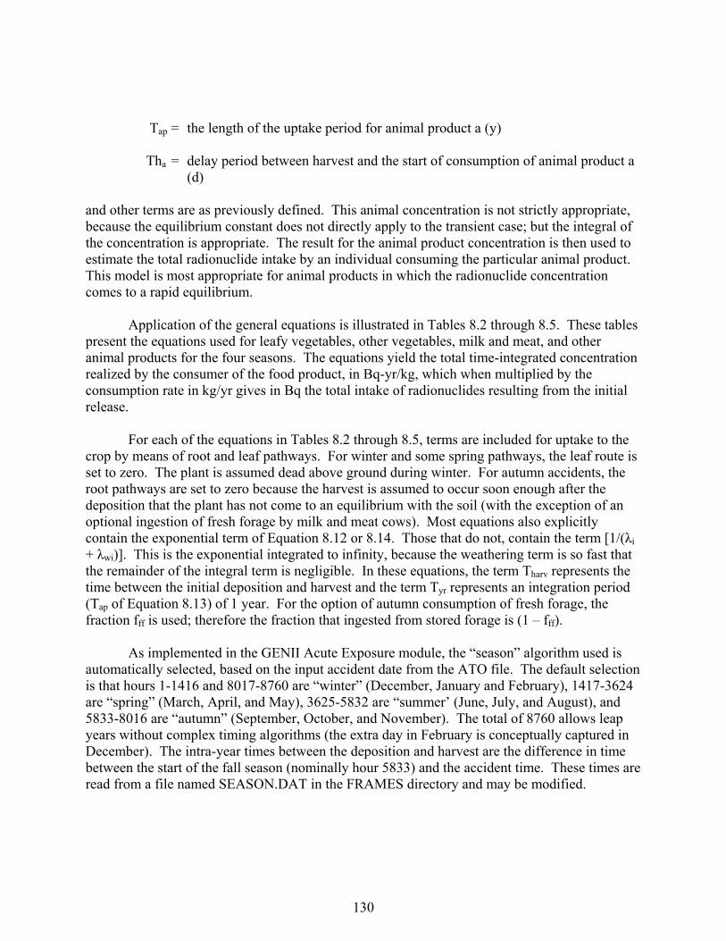
130

Tap = the length of the uptake period for animal product a (y) Tha = delay period between harvest and the start of consumption of animal product a

(d) and other terms are as previously defined. This animal concentration is not strictly appropriate, because the equilibrium constant does not directly apply to the transient case; but the integral of the concentration is appropriate. The result for the animal product concentration is then used to estimate the total radionuclide intake by an individual consuming the particular animal product. This model is most appropriate for animal products in which the radionuclide concentration comes to a rapid equilibrium. Application of the general equations is illustrated in Tables 8.2 through 8.5. These tables present the equations used for leafy vegetables, other vegetables, milk and meat, and other animal products for the four seasons. The equations yield the total time-integrated concentration realized by the consumer of the food product, in Bq-yr/kg, which when multiplied by the consumption rate in kg/yr gives in Bq the total intake of radionuclides resulting from the initial release. For each of the equations in Tables 8.2 through 8.5, terms are included for uptake to the crop by means of root and leaf pathways. For winter and some spring pathways, the leaf route is set to zero. The plant is assumed dead above ground during winter. For autumn accidents, the root pathways are set to zero because the harvest is assumed to occur soon enough after the deposition that the plant has not come to an equilibrium with the soil (with the exception of an optional ingestion of fresh forage by milk and meat cows). Most equations also explicitly contain the exponential term of Equation 8.12 or 8.14. Those that do not, contain the term [1/(λi + λwi)]. This is the exponential integrated to infinity, because the weathering term is so fast that the remainder of the integral term is negligible. In these equations, the term Tharv represents the time between the initial deposition and harvest and the term Tyr represents an integration period (Tap of Equation 8.13) of 1 year. For the option of autumn consumption of fresh forage, the fraction fff is used; therefore the fraction that ingested from stored forage is (1 – fff).

As implemented in the GENII Acute Exposure module, the “season” algorithm used is automatically selected, based on the input accident date from the ATO file. The default selection is that hours 1-1416 and 8017-8760 are “winter” (December, January and February), 1417-3624 are “spring” (March, April, and May), 3625-5832 are “summer’ (June, July, and August), and 5833-8016 are “autumn” (September, October, and November). The total of 8760 allows leap years without complex timing algorithms (the extra day in February is conceptually captured in December). The intra-year times between the deposition and harvest are the difference in time between the start of the fall season (nominally hour 5833) and the accident time. These times are read from a file named SEASON.DAT in the FRAMES directory and may be modified.

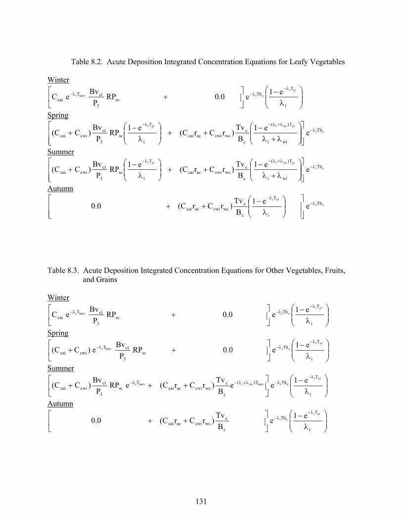
131

Table 8.2. Acute Deposition Integrated Concentration Equations for Leafy Vegetables Winter

i

TTh

sc3

ciTcai

yri

ciharvie1

e0.0RPP

BveC

Spring

ci

yrwiiyriTh

wii

T)(

c

cwccwiaccai

i

T

sc3

cicwicai e

e1

B

Tv)rCrC(

e1RP

P

Bv)CC(

Summer

ci

yrwiiyriTh

wii

T)(

c

cwccwiaccai

i

T

sc3

cicwicai e

e1

B

Tv)rCrC(

e1RP

P

Bv)CC(

Autumn

ci

yriTh

i

T

c

cwccwiaccai e

e1

B

Tv)rCrC(0.0

Table 8.3. Acute Deposition Integrated Concentration Equations for Other Vegetables, Fruits,

and Grains Winter

i

TTh

sc3

ciTcai

yri

ciharvie1

e0.0RPP

BveC

Spring

i

TTh

sc3

ciTcwicai

yri

ciharvie1

e0.0RPP

Bve)CC(

Summer

i

TThT)(

c

cwccwiaccai

Tsc

3

cicwicai

yri

ciharvwiiharvie1

eeB

Tv)rCrC(eRP

P

Bv)CC(

Autumn

i

TTh

c

cwccwiaccai

yri

cie1

eB

Tv)rCrC(0.0

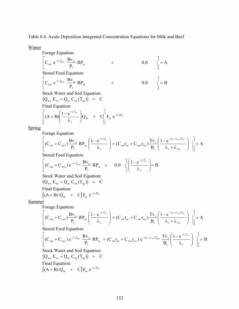
132

Table 8.4. Acute Deposition Integrated Concentration Equations for Milk and Beef Winter Forage Equation:

A0.0RPP

BveC sc

3

ciTcai

harvi

Stored Feed Equation:

B0.0RPP

BveC sc

3

ciTcai

harvi

Stock Water and Soil Equation: C)](TCQE[Q egesisawiwa

Final Equation:

ai

yriTh

aifai

T

eFCQe1

)BA(

Spring Forage Equation:

Ae1

B

Tv)rCrC(

e1RP

P

Bv)CC(

wii

T)(

c

cwccwiaccai

i

T

sc3

cicwicai

yrwiiyri

Stored Feed Equation:

Be1

0.0RPP

Bve)CC(

i

T

sc3

ciTcwicai

yri

harvr

Stock Water and Soil Equation: C)](TCQE[Q egesisawiwa

Final Equation: aiTh

aifa eFCQ)BA(

Summer Forage Equation:

Ae1

B

Tv)rCrC(

e1RP

P

Bv)CC(

wii

T)(

c

cwccwiaccai

i

T

sc3

cicwicai

yrwiiyri

Stored Feed Equation:

Be1

B

Tve)rCrC(RP

P

Bve)CC(

i

T

c

cT)(wccwiaccaisc

3

ciTcwicai

yri

harvwiiharvi

Stock Water and Soil Equation: C)](TCQE[Q egesisawiwa

Final Equation: aiTh

aifa eFCQ)BA(

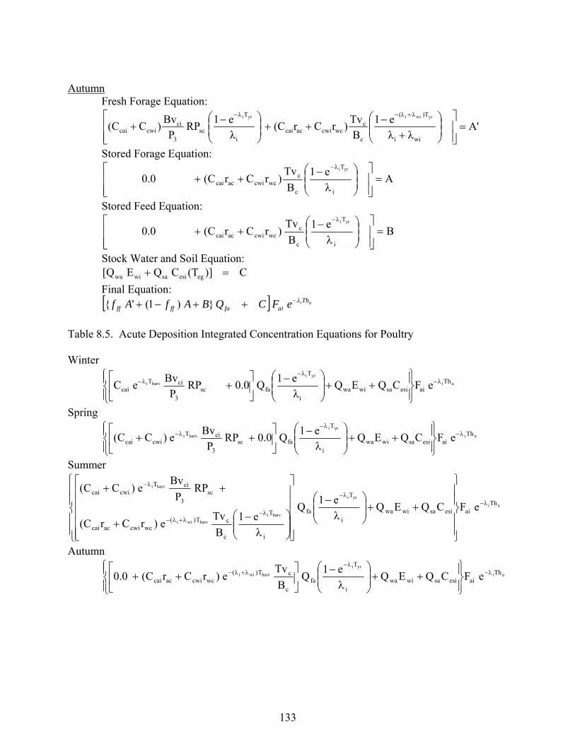
133

Autumn Fresh Forage Equation:

A'λλ

e1

B

Tv)rCr(C

λ

e1RP

P

Bv)C(C

wii

)Tλ(λ

c

cwccwiaccai

i

Tλ

sc3

cicwicai

yrwiiyri

Stored Forage Equation:

Ae1

B

Tv)rCrC(0.0

i

T

c

cwccwiaccai

yri

Stored Feed Equation:

Be1

B

Tv)rCrC(0.0

i

T

c

cwccwiaccai

yri

Stock Water and Soil Equation: C)](TCQE[Q egesisawiwa

Final Equation: aiTh

aifaffff eFCQBAfAf })1('{

Table 8.5. Acute Deposition Integrated Concentration Equations for Poultry Winter

ai

yri

harvi Thλaiesisawiwa

i

Tλ

fasc3

ciTλcai eFCQEQ

λ

e1Q0.0RP

P

BveC

Spring

ai

yri

harvi Thaiesisawiwa

i

T

fasc3

ciTcwicai eFCQEQ

e1Q0.0RP

P

Bve)CC(

Summer

ai

yri

harvi

harvwii

harvi

Thaiesisawiwa

i

T

fa

i

T

c

cT)(wccwiaccai

sc3

ciTcwicai

eFCQEQe1

Qe1

B

Tve)rCrC(

RPP

Bve)CC(

Autumn

ai

yri

harvwii Thaiesisawiwa

i

T

fac

cT)(wccwiaccai eFCQEQ

e1Q

B

Tve)rCrC(0.0

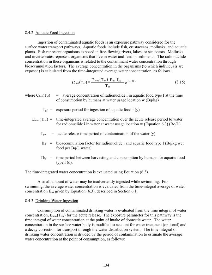
134

8.4.2 Aquatic Food Ingestion Ingestion of contaminated aquatic foods is an exposure pathway considered for the surface water transport pathways. Aquatic foods include fish, crustaceans, mollusks, and aquatic plants. Fish represent organisms exposed in free-flowing rivers, lakes, or sea coasts. Mollusks and invertebrates represent organisms that live in water and feed in sediments. The radionuclide concentration in these organisms is related to the contaminant water concentration through bioaccumulation factors. The average concentration in the organisms (to which individuals are exposed) is calculated from the time-integrated average water concentration, as follows:

where Cfwi(Taf) = average concentration of radionuclide i in aquatic food type f at the time of consumption by humans at water usage location w (Bq/kg)

Taf = exposure period for ingestion of aquatic food f (y) Ewwi(Tew) = time-integrated average concentration over the acute release period to water

for radionuclide i in water at water usage location w (Equation 6.3) (Bq/L) Tew = acute release time period of contamination of the water (y) Bif = bioaccumulation factor for radionuclide i and aquatic food type f (Bq/kg wet

food per Bq/L water) Thf = time period between harvesting and consumption by humans for aquatic food

type f (d). The time-integrated water concentration is evaluated using Equation (6.3). A small amount of water may be inadvertently ingested while swimming. For swimming, the average water concentration is evaluated from the time-integral average of water concentration Ewi given by Equation (6.3), described in Section 6.1. 8.4.3 Drinking Water Ingestion Consumption of contaminated drinking water is evaluated from the time integral of water concentration, Ewwi(Tew) for the acute release. The exposure parameter for this pathway is the time integral of water concentration at the point of intake of domestic water. The water concentration in the surface water body is modified to account for water treatment (optional) and a decay correction for transport through the water distribution system. The time integral of drinking water concentration is divided by the period of contamination to estimate the average water concentration at the point of consumption, as follows:

eT

TB )T(E = )T(C Th -

af

ewif ew wwiaffwi

f i (8.15)

135

where Cdwi(Tdw)= average drinking water concentration of radionuclide i over the acute water release period for water usage location w (Bq/L)

Tdw = period of exposure to the contaminated drinking water (y) TFi = water treatment purification factor giving the fraction of radionuclide i

remaining in the water after treatment (dimensionless) Thd = holdup time between removal of water from the surface water body and

consumption by humans (d). The water concentration time integral at the usage location is evaluated using Equation (6.3). This concentration is also used in the estimation of ingestion intake from inadvertent ingestion during showering. 8.4.4 Inadvertent Soil Ingestion Contamination of soil may occur from atmospheric deposition to soil and waterborne deposition to soil from surface water used for irrigation. The initial concentration in the soil is evaluated using the soil model described for deposition from air or water. The output from the exposure analysis for the soil ingestion pathway is the time integrated soil concentration (per unit mass) evaluated as follows:

where Cdsi(Tsi) = average soil concentration of radionuclide i in soil at soil usage location s over the soil exposure period (Bq/kg)

Csi(t) = concentration of radionuclide i in soil as a function of time following initial

deposition at soil usage location s (Bq/m2) Tsi = exposure period for direct soil ingestion at soil usage location s (y) s = surface soil bulk density (kg/m3) dds = thickness of surface soil layer for the soil ingestion pathway (m).

e T

TF T)T(E = )T(C Th -

dw

i ewew wwidwdwi

d i (8.16)

dt (t)C d T

1 = )T(C si

T

0ds ssisidsi

si

(8.17)

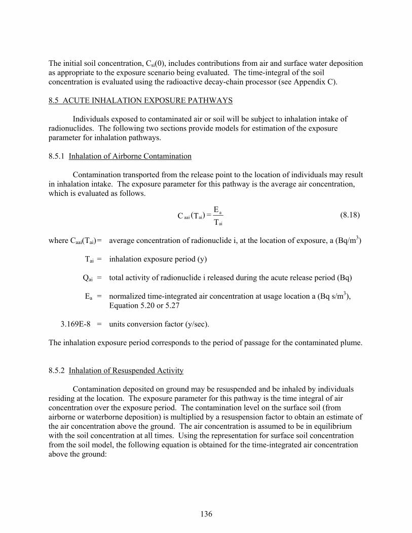
136

The initial soil concentration, Csi(0), includes contributions from air and surface water deposition as appropriate to the exposure scenario being evaluated. The time-integral of the soil concentration is evaluated using the radioactive decay-chain processor (see Appendix C). 8.5 ACUTE INHALATION EXPOSURE PATHWAYS Individuals exposed to contaminated air or soil will be subject to inhalation intake of radionuclides. The following two sections provide models for estimation of the exposure parameter for inhalation pathways. 8.5.1 Inhalation of Airborne Contamination Contamination transported from the release point to the location of individuals may result in inhalation intake. The exposure parameter for this pathway is the average air concentration, which is evaluated as follows.

where Caai(Tai) = average concentration of radionuclide i, at the location of exposure, a (Bq/m3) Tai = inhalation exposure period (y) Qai = total activity of radionuclide i released during the acute release period (Bq) Ea = normalized time-integrated air concentration at usage location a (Bq s/m3),

Equation 5.20 or 5.27 3.169E-8 = units conversion factor (y/sec). The inhalation exposure period corresponds to the period of passage for the contaminated plume. 8.5.2 Inhalation of Resuspended Activity Contamination deposited on ground may be resuspended and be inhaled by individuals residing at the location. The exposure parameter for this pathway is the time integral of air concentration over the exposure period. The contamination level on the surface soil (from airborne or waterborne deposition) is multiplied by a resuspension factor to obtain an estimate of the air concentration above the ground. The air concentration is assumed to be in equilibrium with the soil concentration at all times. Using the representation for surface soil concentration from the soil model, the following equation is obtained for the time-integrated air concentration above the ground:

T

E = )T(C

ai

aaiaai (8.18)

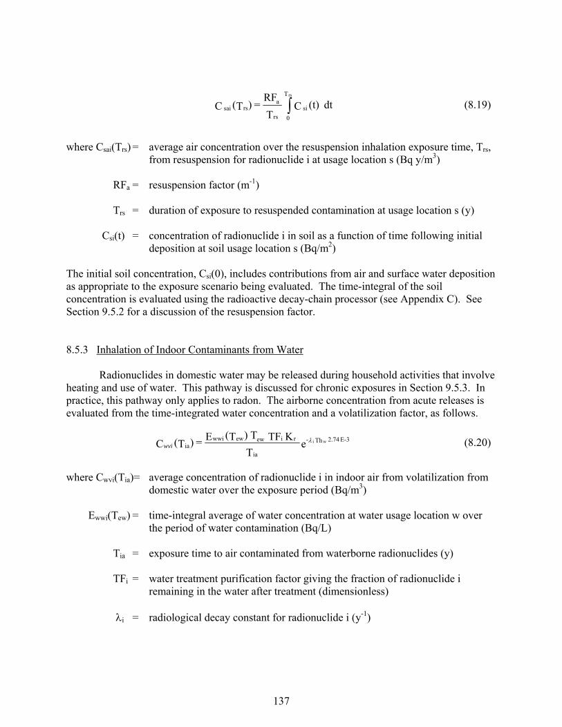
137

where Csai(Trs) = average air concentration over the resuspension inhalation exposure time, Trs, from resuspension for radionuclide i at usage location s (Bq y/m3)

RFa = resuspension factor (m-1) Trs = duration of exposure to resuspended contamination at usage location s (y) Csi(t) = concentration of radionuclide i in soil as a function of time following initial

deposition at soil usage location s (Bq/m2) The initial soil concentration, Csi(0), includes contributions from air and surface water deposition as appropriate to the exposure scenario being evaluated. The time-integral of the soil concentration is evaluated using the radioactive decay-chain processor (see Appendix C). See Section 9.5.2 for a discussion of the resuspension factor. 8.5.3 Inhalation of Indoor Contaminants from Water Radionuclides in domestic water may be released during household activities that involve heating and use of water. This pathway is discussed for chronic exposures in Section 9.5.3. In practice, this pathway only applies to radon. The airborne concentration from acute releases is evaluated from the time-integrated water concentration and a volatilization factor, as follows.

where Cwvi(Tia)= average concentration of radionuclide i in indoor air from volatilization from domestic water over the exposure period (Bq/m3)

Ewwi(Tew) = time-integral average of water concentration at water usage location w over

the period of water contamination (Bq/L) Tia = exposure time to air contaminated from waterborne radionuclides (y) TFi = water treatment purification factor giving the fraction of radionuclide i

remaining in the water after treatment (dimensionless) i = radiological decay constant for radionuclide i (y-1)

dt (t)C T

RF = )T(C si

T

0rs

arssai

rs

(8.19)

eT

K TF T)T(E = )T(C 3E-2.74 Th -

ia

riewewwwiia

wiwvi (8.20)

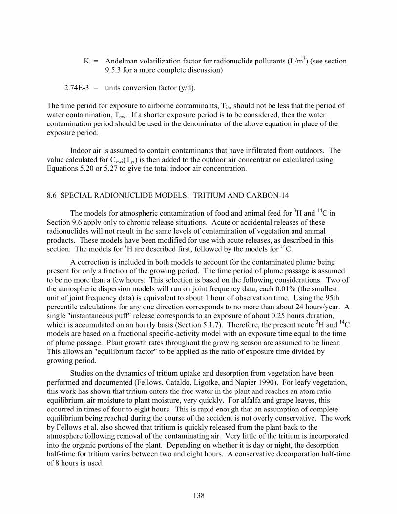
138

Kr = Andelman volatilization factor for radionuclide pollutants (L/m3) (see section 9.5.3 for a more complete discussion)

2.74E-3 = units conversion factor (y/d). The time period for exposure to airborne contaminants, Tia, should not be less that the period of water contamination, Tew. If a shorter exposure period is to be considered, then the water contamination period should be used in the denominator of the above equation in place of the exposure period. Indoor air is assumed to contain contaminants that have infiltrated from outdoors. The value calculated for Cvwi(Tyr) is then added to the outdoor air concentration calculated using Equations 5.20 or 5.27 to give the total indoor air concentration. 8.6 SPECIAL RADIONUCLIDE MODELS: TRITIUM AND CARBON-14 The models for atmospheric contamination of food and animal feed for 3H and 14C in Section 9.6 apply only to chronic release situations. Acute or accidental releases of these radionuclides will not result in the same levels of contamination of vegetation and animal products. These models have been modified for use with acute releases, as described in this section. The models for 3H are described first, followed by the models for 14C.

A correction is included in both models to account for the contaminated plume being present for only a fraction of the growing period. The time period of plume passage is assumed to be no more than a few hours. This selection is based on the following considerations. Two of the atmospheric dispersion models will run on joint frequency data; each 0.01% (the smallest unit of joint frequency data) is equivalent to about 1 hour of observation time. Using the 95th percentile calculations for any one direction corresponds to no more than about 24 hours/year. A single "instantaneous puff" release corresponds to an exposure of about 0.25 hours duration, which is accumulated on an hourly basis (Section 5.1.7). Therefore, the present acute 3H and 14C models are based on a fractional specific-activity model with an exposure time equal to the time of plume passage. Plant growth rates throughout the growing season are assumed to be linear. This allows an "equilibrium factor" to be applied as the ratio of exposure time divided by growing period.

Studies on the dynamics of tritium uptake and desorption from vegetation have been performed and documented (Fellows, Cataldo, Ligotke, and Napier 1990). For leafy vegetation, this work has shown that tritium enters the free water in the plant and reaches an atom ratio equilibrium, air moisture to plant moisture, very quickly. For alfalfa and grape leaves, this occurred in times of four to eight hours. This is rapid enough that an assumption of complete equilibrium being reached during the course of the accident is not overly conservative. The work by Fellows et al. also showed that tritium is quickly released from the plant back to the atmosphere following removal of the contaminating air. Very little of the tritium is incorporated into the organic portions of the plant. Depending on whether it is day or night, the desorption half-time for tritium varies between two and eight hours. A conservative decorporation half-time of 8 hours is used.

139

The concentration in air during the period of plume passage is evaluated from the time-integrated average air concentration as follows.

where CcaH = average tritium concentration in air during the period of plume passage at the location of crop type c (Bq/m3)

Ec = time-integrated average air concentration at crop growing location c

(Equations 5.20 or 5.27), which incorporates the complete time of the release and plume passage Te, (Bq/m3)

During the period of plume passage the plant is assumed to attain equilibrium with tritium in environmental water. The basic models describing uptake and incorporation as organically-bound tritium (OBT) are described in Section 9.6. For both plants and the animals that eat them, the tritium is assumed to decorporate according to the 8 hour retention half-time. The infinite integral of concentration is equal to 1/ = 8 h / ln 2 times the peak tritium concentration. Releases of elemental tritium gas (HT) are a special case. Hydrogen in the elemental form is not readily taken up into vegetation. However, HT is slowly oxidized into tritiated water (HTO) by microbes in soil. For experiments at Chalk River that ran to equilibrium, Peterson and Davis (2002) found an empirical relationship of 8Bq L-1 /(Bq m-3) for the ratio of HTO in air moisture to HT in air. This is used here as a simple approximation for the time integrated result (personal communication, S.-R. Peterson). This allows a simple addition to the model described above, in which all terms remain the same if CcaH is approximated as 8 CcaHT H (where H is the absolute humidity). Uptake of 14C into plants is assumed via photosynthesis. Thus, the model assumes carbon behaves as CO2. It is assumed that any new growth fixes 14C and 12C at ratios the same as in the air during the passage of the plume. However, only a small portion of the total biomass of the plant would be fixed during the acute plume passage period. Therefore, an approximation to the attained concentration is obtained by using the specific-activity approach times the fraction of the growing period represented by plume passage. This technique is the same as others described in this report, because the other approaches all use the time-integrated air concentration, independent of time. Likewise, the 14C model does not require a discrete time and peak concentration. The concentration in plants from atmospheric transport is evaluated by first calculating the average concentration in the air above the plant during the period of plume passage, as for tritium.

ccaH E = C (8.21)

140

where CacC = concentration of carbon-14 in air at the growing location of crop type c (Bq/m3)

Ea = time-integrated air concentration at usage location a (Equations 5.20 or 5.27),

which incorporates the complete time of the release and plume passage Te, (Bq sec/m3)

The concentration fixed in the plant leaves during this period is in equilibrium with this air concentration and is evaluated as follows.

where Ccai(0) = concentration in the plant at the time of harvest for crop c from airborne deposition (Bq/kg wet weight)

FCc = fraction of carbon in crop type c (dimensionless) PC = concentration of carbon in air (kg/m3) EC = equilibrium factor for carbon (dimensionless). The equilibrium factor is evaluated as described above and by the following equation.

where Tpp = period of plume passage, assumed equal to Te (hr) Tgc = growing period for crop type c (d) 24 = units conversion factor (hr/d). The plant concentration from irrigation with 14C contaminated water is based on the assumption that no more than 10% of the carbon in a plant comes from root uptake from soil and that no carbon is taken up from water on the plant leaves. Also, no more than 1% of soil is assumed to be carbon. All carbon entering the plant is assumed to be fixed with no subsequent loss. The irrigation deposition rate to soil is used to estimate the 14C concentration in soil at the time of deposition. The deposition is assumed to occur just prior to the harvest so there is no loss of 14C from soil before harvest. This soil concentration is then used to estimate the plant concentration from root uptake. The deposition onto soil via irrigation is modeled as follows.

aacC E = C (8.22)

P

E F C = (0)CC

CCcacCca i (8.23)

24 T

T = Egc

ppC (8.24)

141

where CscC(0) = concentration of 14C in soil used for crop type c at the time of contamination deposition from irrigation water (Bq/kg soil)

CwC = average water concentration of 14C in irrigation water, over the time of use of

the contaminated water (Bq/L) IRww = irrigation rate (L./m2 sec) Tw = time of plume passage (s) P3 = areal soil density of surface soil (kg/m2). The average water concentration is evaluated using Equation (6.3). The plant is assumed to be in equilibrium with this soil concentration using the assumptions mentioned above, as follows.

where CcwC(0) = concentration on the plant at the time of harvest for crop c from irrigation water deposition (Bq/kg wet weight)

0.1 = fraction of carbon in a plant that is assumed to come via roots (dimensionless) 0.01 = fraction of soil that is carbon (kg C in soil/kg soil) FCc = fraction of carbon in crop type c (dimensionless). There is assumed to be no loss of 14C from the plant after harvest. Therefore, the harvest concentration persists throughout the consumption period. The concentration of 14C in animal products is based on animal ingestion of contaminated feed (carbon uptake via drinking water is negligible). The feed concentrations are estimated using Equation (8.26) or (8.29) with parameters defined for the feed crop. The animal product concentration is evaluated as follows.

P

TIR C = (0)C3

wwwCscC (8.25)

0.01F 0.1 (0)C = (0)C

cCscCcwC (8.26)

142

where CawC(0) = concentration of 14C in animal product a at time of harvest (Bq/kg) FCa = fraction of carbon in animal product a (dimensionless) CfwC = concentration of 14C in animal feed type f at time of animal feed

consumption, immediately after contamination (Bq/kg wet weight) Uaf = daily intake rate for animal type a of feed type f (kg/d) daf = fraction of animal type a feed type f intake that is contaminated

(dimensionless) FCf = fraction of carbon in animal feed type f (dimensionless) Nfa = number of feed crops eaten by animal type a. There is assumed to be no loss of carbon-14 after animal products production, so the production concentration persists throughout the consumption period. 8.7 REFERENCES FOR SECTION 8 Baes, C. F., and R. D. Sharp. 1981. Predicting Radionuclide Leaching From Root Zone Soil From Assessment Applications. CONF-81606, Oak Ridge National Laboratory, Oak Ridge, Tennessee. Fellows, R.J., D.A. Cataldo, M.W. Ligotke, and B.A. Napier. 1990. Transfer of Atmospheric Tritiated Water to Foliage and Fruit of Crops, PNL-7521, Pacific Northwest Laboratory, Richland, Washington. Govaerts, P., I. Mertens, and J. G. Kretzschmer. 1983. Application of the DOSDIM-Model to Assess Doses Due to Deposited Materials Subsequent to an Accidental Atmospheric Release. Studiecentrum voor Kernenergie, Mol, Belgium. Napier, B. A, R. A. Peloquin, D. L. Strenge, and J. V. Ramsdell. 1988. HANFORD ENVIRONMENTAL DOSIMETRY UPGRADE PROJECT. GENII - The Hanford Environmental Radiation Dosimetry Software System. Volume 1: Conceptual Representation, Volume 2: Users' Manual, Volume 3: Code Maintenance Manual. PNL-6584, Vols. 1-3, Pacific Northwest Laboratory, Richland, Washington.

U F

d U C F = (0)C

afCa

N

1=f

afaffwC

N

1=fCaawC

fa

fa

(8.27)

143

Nelson, J. L. 1965. "Distribution of Sediments and Associated Radionuclides in the Columbia River Below Hanford." In Hanford Radiological Sciences Research and Development Report for 1964, ed. D. W. Reece and J. K. Green, p. 3.80. USAEC Report BNWL-36, Pacific Northwest Laboratory, Richland, Washington. Peterson, S.-R., and P.A. Davis. 2001. “Tritium Doses from Chronic Atmospheric Releases: A New Method Proposed for Regulatory Compliance,” Health Physics, 82(2):213-225. Soldat, J. K., N. M. Robinson and D. A. Baker. 1974. Models and Computer Codes for Evaluating Environmental Radiation Doses. BNWL-1754. Battelle, Pacific Northwest Laboratory, Richland, Washington. Toombs, G. L., and P. B. Cutler, eds. 1968. Comprehensive Final Report for the Lower Columbia River Environmental Survey in Oregon, June 5, 1961 - July 31, 1967. Oregon State Board of Health, Division of Sanitation and Engineering, Salem, Oregon. Whicker, F. W., and T. B. Kirchner. 1987. "PATHWAY: A Dynamic Foodchain Model to Predict Radionuclide Ingestion After Fallout Deposition." Health Physics 52:717-738.

144

9.0 CHRONIC EXPOSURE MODULE

The chronic exposure module provides estimates of exposure media concentrations resulting from groundwater, surface water, and airborne contamination pathways. Exposures are treated as continuous and constant over an extended time period (a year or longer) with consideration of the time variation in air and water concentrations from year to year. In this section, the communication interfaces are described first, followed by the exposure pathway models for external exposure, ingestion exposure, and inhalation exposure. The chronic exposure module uses as input radionuclide concentrations in air and water, as generated by the transport models or from user defined input. The output from the module is the radionuclide concentration in various exposure media (air, crops, animal products, soil, aquatic foods, etc.). The exposure pathways considered by the chronic module are indicated in Table 9.1. Model details are given in following sections. Table 9.1 Exposure Pathways for the Chronic Terrestrial and Aquatic Module Transport Mode Exposure Pathways Exposure Route atmosphere air inhalation soil resuspension inhalation soil ingestion ingestion immersion in air external ground exposure external food crops ingestion animal products ingestion groundwater drinking water ingestion shower volatilization inhalation irrigated food crops ingestion irrigation/animal products ingestion ground exposure external surface water drinking water ingestion shower volatilization inhalation shower water ingestion ingestion irrigated food crops ingestion irrigation/animal products ingestion ground exposure external swimming external swimming water ingestion ingestion boating external shoreline sediment external aquatic foods ingestion soil contamination soil resuspension inhalation soil ingestion ingestion ground exposure external

145

9.1 COMMUNICATION INTERFACES The input files for the chronic exposure module are the global input data file (GID), the atmospheric concentration file (ATO), the water concentration file (WCF), and one auxiliary data communication file (radionuclide master date library). The communication interfaces are indicated in Figure 9.1. The atmospheric concentration file (ATO) is generated by the atmospheric transport module. The water concentration file (WCF) is generated by the surface water module (or other external program that is capable of generating the water concentration file information). The GID file section for the chronic exposure module is generated by the user interface program. It contains information describing the scope of the analysis and all user-provided input parameters for an analysis. The structure and content of the files are given in Appendix A and B. The output from the chronic terrestrial and aquatic pathway module is the concentration in various media to which individuals or populations are exposed. Along with each concentration, the duration of exposure is also provided, representing the period of integration for the particular pathway. This information is provided in a primary data communication file, the exposure pathway media concentration output file (EPF). ••••••••••••••• • Radionuclide• • Master Data • • Library • ••••••••••••••• •••••••••• • ••••••••••••••••• • • • • Atmospheric • •Global • • • Transport • •Input • ••••••••••••••••••••••••••••••••••••• • Output File • •Data •••••••• Chronic Terrestrial and Aquatic •••••••• (ATO) • •File • • Transfer and Accumulation • ••••••••••••••••• •(GID) • • Calculational Component • ••••••••••••••••• • • • •••••••• Water • • • ••••••••••••••••••••••••••••••••••••• • Concentration • • • • • Output File • •••••••••• •••••••••••••••••••••••••••• • (WCF) • • Exposure Pathway Media • ••••••••••••••••• • Concentration Output • • File (EPF) • ••••••••••••••••••••••••••••

Figure 9.1 Communication Interfaces for the Chronic Pathway Component

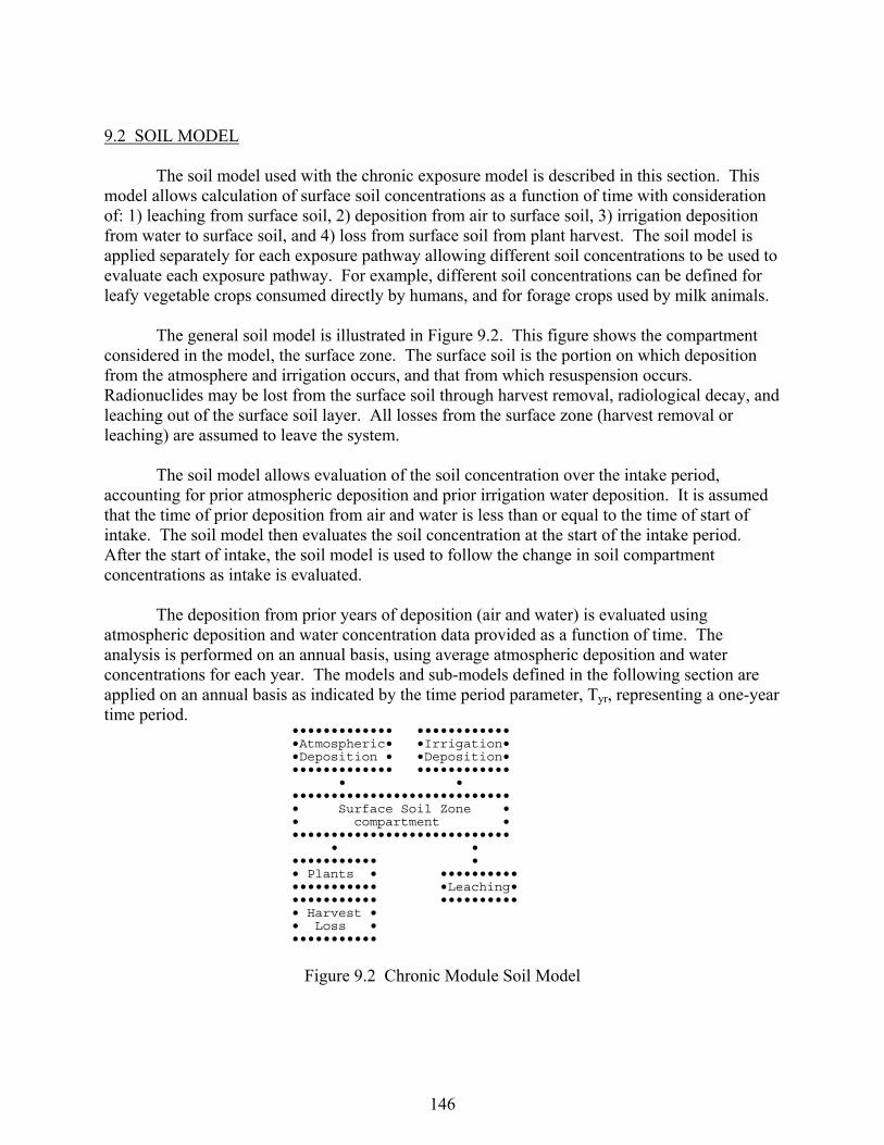
146

9.2 SOIL MODEL The soil model used with the chronic exposure model is described in this section. This model allows calculation of surface soil concentrations as a function of time with consideration of: 1) leaching from surface soil, 2) deposition from air to surface soil, 3) irrigation deposition from water to surface soil, and 4) loss from surface soil from plant harvest. The soil model is applied separately for each exposure pathway allowing different soil concentrations to be used to evaluate each exposure pathway. For example, different soil concentrations can be defined for leafy vegetable crops consumed directly by humans, and for forage crops used by milk animals. The general soil model is illustrated in Figure 9.2. This figure shows the compartment considered in the model, the surface zone. The surface soil is the portion on which deposition from the atmosphere and irrigation occurs, and that from which resuspension occurs. Radionuclides may be lost from the surface soil through harvest removal, radiological decay, and leaching out of the surface soil layer. All losses from the surface zone (harvest removal or leaching) are assumed to leave the system. The soil model allows evaluation of the soil concentration over the intake period, accounting for prior atmospheric deposition and prior irrigation water deposition. It is assumed that the time of prior deposition from air and water is less than or equal to the time of start of intake. The soil model then evaluates the soil concentration at the start of the intake period. After the start of intake, the soil model is used to follow the change in soil compartment concentrations as intake is evaluated. The deposition from prior years of deposition (air and water) is evaluated using atmospheric deposition and water concentration data provided as a function of time. The analysis is performed on an annual basis, using average atmospheric deposition and water concentrations for each year. The models and sub-models defined in the following section are applied on an annual basis as indicated by the time period parameter, Tyr, representing a one-year time period. ••••••••••••• •••••••••••• •Atmospheric• •Irrigation• •Deposition • •Deposition• ••••••••••••• •••••••••••• • • •••••••••••••••••••••••••••• • Surface Soil Zone • • compartment • •••••••••••••••••••••••••••• • • ••••••••••• • • Plants • •••••••••• ••••••••••• •Leaching• ••••••••••• •••••••••• • Harvest • • Loss • •••••••••••

Figure 9.2 Chronic Module Soil Model

147

The model is defined by a differential equation that describes the change of concentration in surface soil as a function of time. The differential equation for the soil model compartment is defined in terms of the amount of each radionuclide chain member present in units of atoms. This representation is used for ease of understanding and ease of solving the equations. The final solutions are evaluated using the radioactive decay-chain processor described in Appendix C. The general solutions presented in that appendix are given in terms of atom units and activity units. For chronic releases, initial amount in the surface soil is set to zero. The decrease from harvest is modeled as a step function following the time of harvest and does not appear in the differential equation for the surface zone. The differential equation for chronic releases for the surface soil zone is as follows:

where Ai(t) = amount of radionuclide i in the surface soil zone at time, t (atoms) Rwi = rate of input from irrigation water (atoms /y) Rai = rate of input from atmospheric depostion (atoms/y) i = rate constant for radioactive decay of radionuclide i (y-1) Li = rate constant for leaching of radionuclide from the surface soil zone (y-1). Various aspects of the soil model are described in the following subsections. The first section describes definition of air and water deposition during a year for chronic releases. The remaining sections describe estimation methods for the transfer rate constants defined for the soil model. 9.2.1 Activity from Air and Water Deposition For chronic release analyses the differential equation for surface soil includes terms for deposition from air and irrigation water. The initial concentrations are set to be zero. The amount at the end of a year is evaluated based on the amount present at the beginning of a year plus the amount deposited during the year. In the exposure pathway models that follow, the amount present during a year is composed of two terms: 1) the average amount present during the year from prior years’ depositions, and 2) the average amount present from deposited during the year. The average amount present from prior years’ contributions is represented by the term Csi(Tyr) with units of Bq/m2. This amount is evaluated from the amount present at the end of the prior year (corrected as necessary according to soil model transfers), and accounting for radioactive decay and losses during the year. These evaluations are made using the decay processor described in Appendix C. The deposition during the current year is evaluated as defined for each exposure pathway.

A ) + ( - )R + R( = td

(t)A diiLii ai

i w (9.1)

148

9.2.2 Leaching from the Surface Soil Zone Removal from the surface soils through leaching into deeper soils is treated by means of a soil removal rate constant. For surface soils the rate constant, si, is a correction for long-term leaching of deposited radionuclides out of the surface soil (rooting and resuspension zones). The values for si are calculated using the formula of Baes and Sharp (1981):

where si = removal rate constant for activity of radionuclide i in the surface soil layer (y-1) P = total annual precipitation (cm/y) I = total irrigation rate (cm/y) E = total evapotranspiration rate (cm/y) s = surface soil bulk density (kg/m3) s = surface soil volumetric water content (mL/cm3) Kdsi = surface soil distribution coefficient for radionuclide i (mL/g) 10-2 = units conversion factor (m/cm) 103 = units conversion factor (g/kg) 10-6 = units conversion factor (m3/ml) ds = depth of surface layer (cm) 9.2.3 Loss by Harvest Loss of activity from the surface soil zone is modeled as a step function applied at the end of each calculational year. The amount of loss is calculated from the plant concentration at harvest, the annual plant yield, and the soil concentrations at harvest. The calculation is represented by the following equation.

where Csi(t+) = surface soil concentration at soil location s for radionuclide i after correction for harvest removal at time t (Bq/m2)

Csi(t-) = surface soil concentration at soil location s for radionuclide i before correction

for harvest removal at time t (Bq/m2)

Kd

10 10 + 1 d

E) - I + (P 10 =

sis

s6-3

ss

-2

si

(9.2)

C/Y )Th(C - C)t(C = )t(C sic ci ch si-si+si (9.3)

149

Chci(Thc) = crop c concentration for radionuclide i at time of harvest (Bq/kg) Yc = annual yield of crop c (kg/m2) The multiplicative term represents the average fraction of the contaminant in soil to that in crops over the year; this term is used rather than a simple subtraction of amount harvested because, for short-lived radionuclides, the amount harvested over the year may actually be larger than the amount remaining in the soil at the end of the year. 9.3 EXTERNAL EXPOSURE PATHWAYS External exposures from atmospheric transport include immersion in air and exposure to contaminated ground following deposition from air. External exposure from groundwater transport involves ground contamination from irrigation deposition. External exposure from surface water transport includes ground contamination from irrigation deposition, swimming in contaminated water, boating on contaminated water, and exposure to shoreline sediment contaminated by transfer from surface water. Models for evaluating these exposure pathways are provided here. 9.3.1 External Plume Immersion External exposure from immersion in a plume is evaluated in the atmospheric transport component and provided to subsequent components as the radiation dose (Sv) received during plume passage at specific locations. As such, no models need to be described in this section. The evaluation of radiation dose is performed using the finite dimensions of the plume. However, an alternate method for evaluating external exposure is described here using the semi-infinite plume model, which does not require knowledge of plume dimension. The model uses the average air concentration over the exposure period to estimate dose. The input parameter for estimation of external exposure to the plume using the semi-infinite plume model is the average air concentration of a radionuclide in the plume, as estimated by the atmospheric transport component, nv = Cai = air concentration for radionuclide i at usage location a (Bq/m3) from Equations 5.19 or 5.28. 9.3.2 External Ground Exposure External exposure to contaminated ground is considered for atmospheric transport and deposition, for groundwater and surface water irrigation, and deposition from these sources from prior years’ activity. The annual average value is used (requiring a time integral equation). The exposure parameter for this pathway is the average soil concentration over the year of exposure in units of Bq/m2. If the exposure parameter is divided by the soil areal density, then the units are in Bq/kg. The soil concentration used in evaluation of the external exposure is

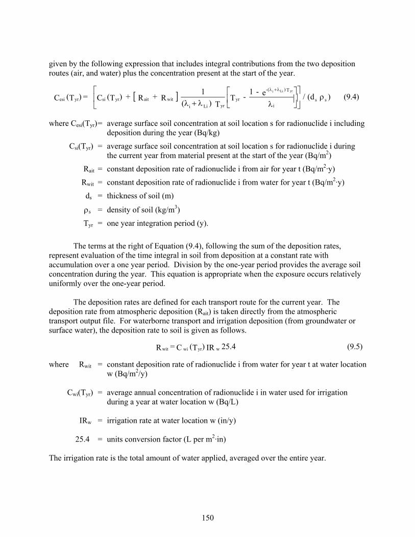
150

given by the following expression that includes integral contributions from the two deposition routes (air, and water) plus the concentration present at the start of the year.

where Cesi(Tyr) = average surface soil concentration at soil location s for radionuclide i including deposition during the year (Bq/kg)

Csi(Tyr) = average surface soil concentration at soil location s for radionuclide i during the current year from material present at the start of the year (Bq/m2)

Rait = constant deposition rate of radionuclide i from air for year t (Bq/m2·y)

Rwit = constant deposition rate of radionuclide i from water for year t (Bq/m2·y)

ds = thickness of soil (m)

s = density of soil (kg/m3)

Tyr = one year integration period (y).

The terms at the right of Equation (9.4), following the sum of the deposition rates, represent evaluation of the time integral in soil from deposition at a constant rate with accumulation over a one year period. Division by the one-year period provides the average soil concentration during the year. This equation is appropriate when the exposure occurs relatively uniformly over the one-year period. The deposition rates are defined for each transport route for the current year. The deposition rate from atmospheric deposition (Rait) is taken directly from the atmospheric transport output file. For waterborne transport and irrigation deposition (from groundwater or surface water), the deposition rate to soil is given as follows.

where Rwit = constant deposition rate of radionuclide i from water for year t at water location w (Bq/m2/y)

Cwi(Tyr) = average annual concentration of radionuclide i in water used for irrigation

during a year at water location w (Bq/L) IRw = irrigation rate at water location w (in/y) 25.4 = units conversion factor (L per m2·in) The irrigation rate is the total amount of water applied, averaged over the entire year.

)d(/e - 1 - T

T )(

1 R + R + )T( C = )T( C ss

i

T ) (-

yryrLii

witaityrsiyresi

yrLii

(9.4)

25.4 IR )T( C = R wyr wiwit (9.5)

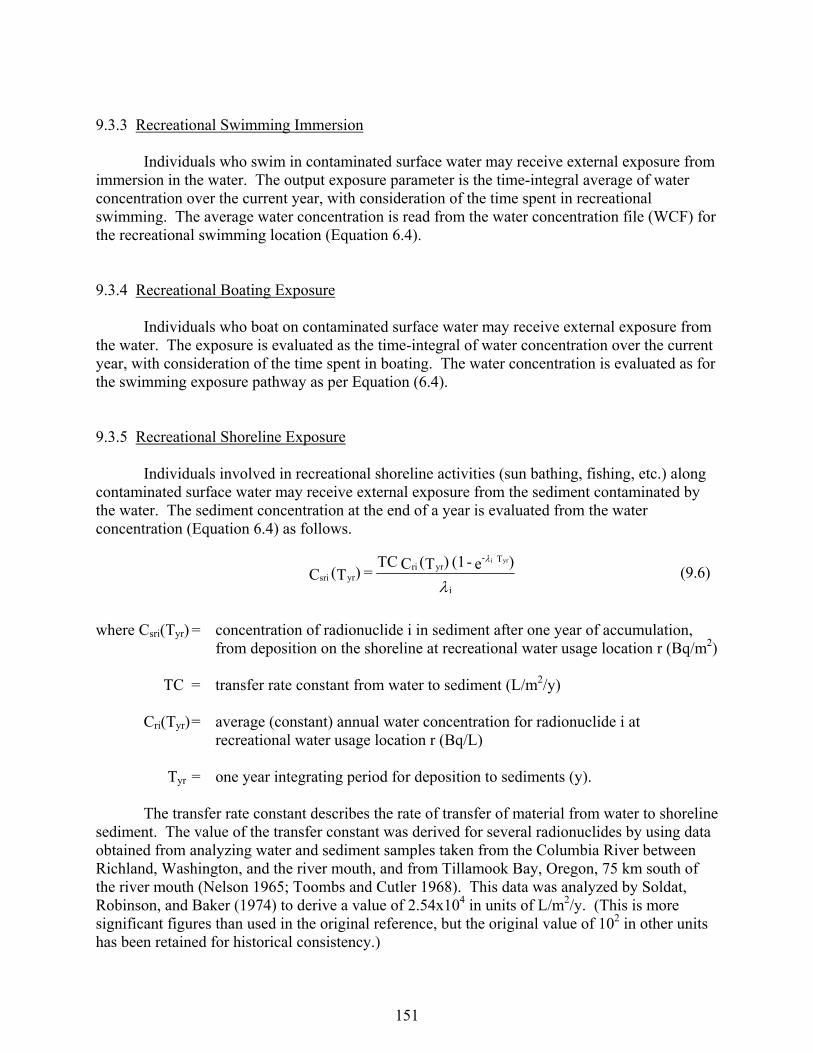
151

9.3.3 Recreational Swimming Immersion Individuals who swim in contaminated surface water may receive external exposure from immersion in the water. The output exposure parameter is the time-integral average of water concentration over the current year, with consideration of the time spent in recreational swimming. The average water concentration is read from the water concentration file (WCF) for the recreational swimming location (Equation 6.4). 9.3.4 Recreational Boating Exposure Individuals who boat on contaminated surface water may receive external exposure from the water. The exposure is evaluated as the time-integral of water concentration over the current year, with consideration of the time spent in boating. The water concentration is evaluated as for the swimming exposure pathway as per Equation (6.4). 9.3.5 Recreational Shoreline Exposure Individuals involved in recreational shoreline activities (sun bathing, fishing, etc.) along contaminated surface water may receive external exposure from the sediment contaminated by the water. The sediment concentration at the end of a year is evaluated from the water concentration (Equation 6.4) as follows.

where Csri(Tyr) = concentration of radionuclide i in sediment after one year of accumulation, from deposition on the shoreline at recreational water usage location r (Bq/m2)

TC = transfer rate constant from water to sediment (L/m2/y) Cri(Tyr) = average (constant) annual water concentration for radionuclide i at

recreational water usage location r (Bq/L) Tyr = one year integrating period for deposition to sediments (y). The transfer rate constant describes the rate of transfer of material from water to shoreline sediment. The value of the transfer constant was derived for several radionuclides by using data obtained from analyzing water and sediment samples taken from the Columbia River between Richland, Washington, and the river mouth, and from Tillamook Bay, Oregon, 75 km south of the river mouth (Nelson 1965; Toombs and Cutler 1968). This data was analyzed by Soldat, Robinson, and Baker (1974) to derive a value of 2.54x104 in units of L/m2/y. (This is more significant figures than used in the original reference, but the original value of 102 in other units has been retained for historical consistency.)

i

T -yrri

yrsri

)e - (1 )T(C TC = )T(C

yri

(9.6)

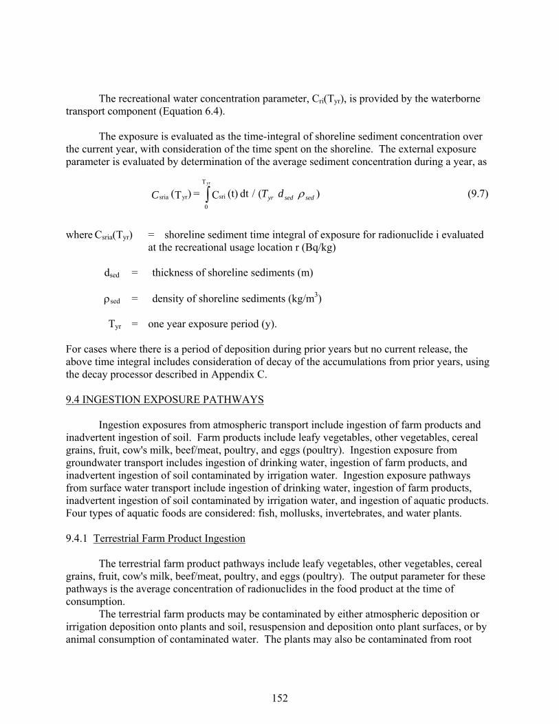
152

The recreational water concentration parameter, Cri(Tyr), is provided by the waterborne transport component (Equation 6.4). The exposure is evaluated as the time-integral of shoreline sediment concentration over the current year, with consideration of the time spent on the shoreline. The external exposure parameter is evaluated by determination of the average sediment concentration during a year, as

where Csria(Tyr) = shoreline sediment time integral of exposure for radionuclide i evaluated at the recreational usage location r (Bq/kg)

dsed = thickness of shoreline sediments (m) sed = density of shoreline sediments (kg/m3) Tyr = one year exposure period (y). For cases where there is a period of deposition during prior years but no current release, the above time integral includes consideration of decay of the accumulations from prior years, using the decay processor described in Appendix C. 9.4 INGESTION EXPOSURE PATHWAYS Ingestion exposures from atmospheric transport include ingestion of farm products and inadvertent ingestion of soil. Farm products include leafy vegetables, other vegetables, cereal grains, fruit, cow's milk, beef/meat, poultry, and eggs (poultry). Ingestion exposure from groundwater transport includes ingestion of drinking water, ingestion of farm products, and inadvertent ingestion of soil contaminated by irrigation water. Ingestion exposure pathways from surface water transport include ingestion of drinking water, ingestion of farm products, inadvertent ingestion of soil contaminated by irrigation water, and ingestion of aquatic products. Four types of aquatic foods are considered: fish, mollusks, invertebrates, and water plants. 9.4.1 Terrestrial Farm Product Ingestion The terrestrial farm product pathways include leafy vegetables, other vegetables, cereal grains, fruit, cow's milk, beef/meat, poultry, and eggs (poultry). The output parameter for these pathways is the average concentration of radionuclides in the food product at the time of consumption. The terrestrial farm products may be contaminated by either atmospheric deposition or irrigation deposition onto plants and soil, resuspension and deposition onto plant surfaces, or by animal consumption of contaminated water. The plants may also be contaminated from root

)(/dt (t) C = )T( sri

T

0

yrsria

yr

sedsedyr dTC (9.7)

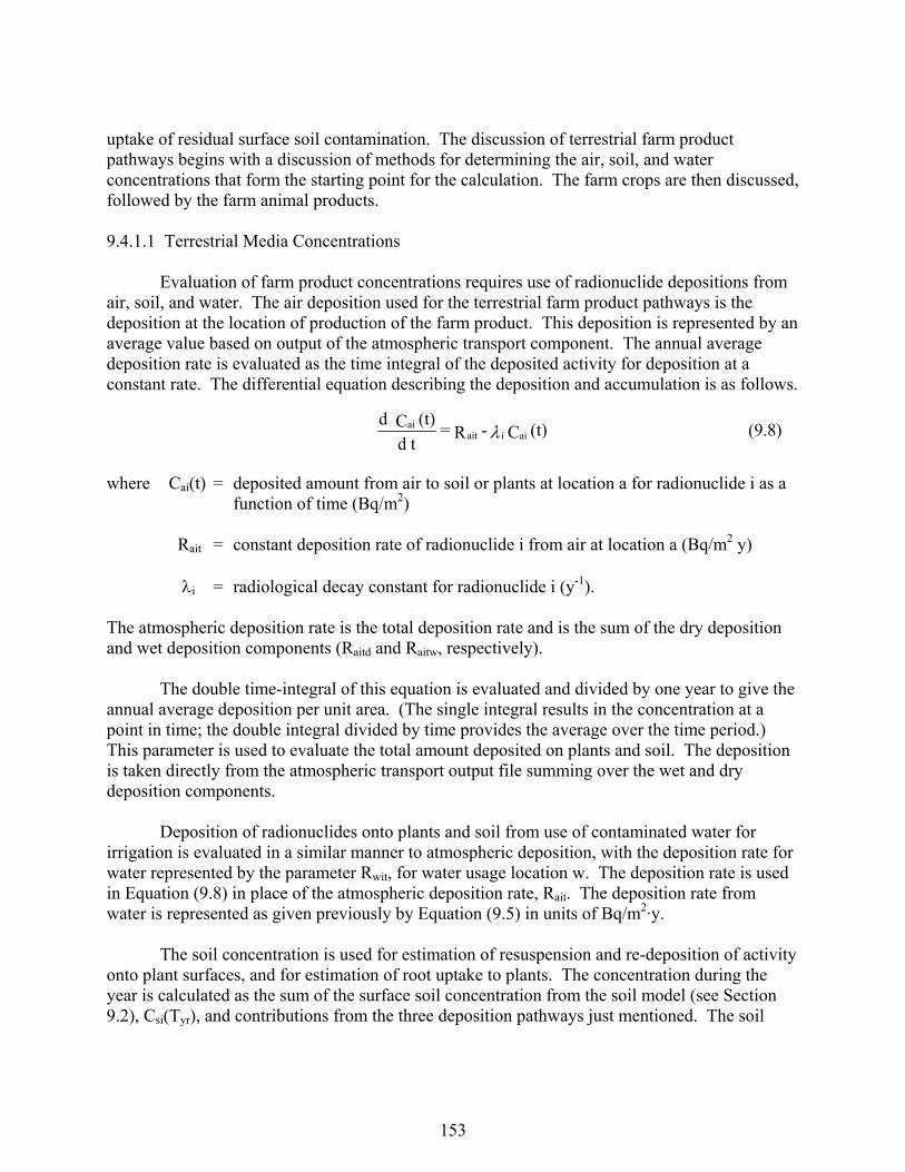
153

uptake of residual surface soil contamination. The discussion of terrestrial farm product pathways begins with a discussion of methods for determining the air, soil, and water concentrations that form the starting point for the calculation. The farm crops are then discussed, followed by the farm animal products. 9.4.1.1 Terrestrial Media Concentrations Evaluation of farm product concentrations requires use of radionuclide depositions from air, soil, and water. The air deposition used for the terrestrial farm product pathways is the deposition at the location of production of the farm product. This deposition is represented by an average value based on output of the atmospheric transport component. The annual average deposition rate is evaluated as the time integral of the deposited activity for deposition at a constant rate. The differential equation describing the deposition and accumulation is as follows.

where Cai(t) = deposited amount from air to soil or plants at location a for radionuclide i as a function of time (Bq/m2)

Rait = constant deposition rate of radionuclide i from air at location a (Bq/m2 y) i = radiological decay constant for radionuclide i (y-1). The atmospheric deposition rate is the total deposition rate and is the sum of the dry deposition and wet deposition components (Raitd and Raitw, respectively). The double time-integral of this equation is evaluated and divided by one year to give the annual average deposition per unit area. (The single integral results in the concentration at a point in time; the double integral divided by time provides the average over the time period.) This parameter is used to evaluate the total amount deposited on plants and soil. The deposition is taken directly from the atmospheric transport output file summing over the wet and dry deposition components. Deposition of radionuclides onto plants and soil from use of contaminated water for irrigation is evaluated in a similar manner to atmospheric deposition, with the deposition rate for water represented by the parameter Rwit, for water usage location w. The deposition rate is used in Equation (9.8) in place of the atmospheric deposition rate, Rait. The deposition rate from water is represented as given previously by Equation (9.5) in units of Bq/m2·y. The soil concentration is used for estimation of resuspension and re-deposition of activity onto plant surfaces, and for estimation of root uptake to plants. The concentration during the year is calculated as the sum of the surface soil concentration from the soil model (see Section 9.2), Csi(Tyr), and contributions from the three deposition pathways just mentioned. The soil

(t) C - R = td

(t) C daiiait

ai (9.8)

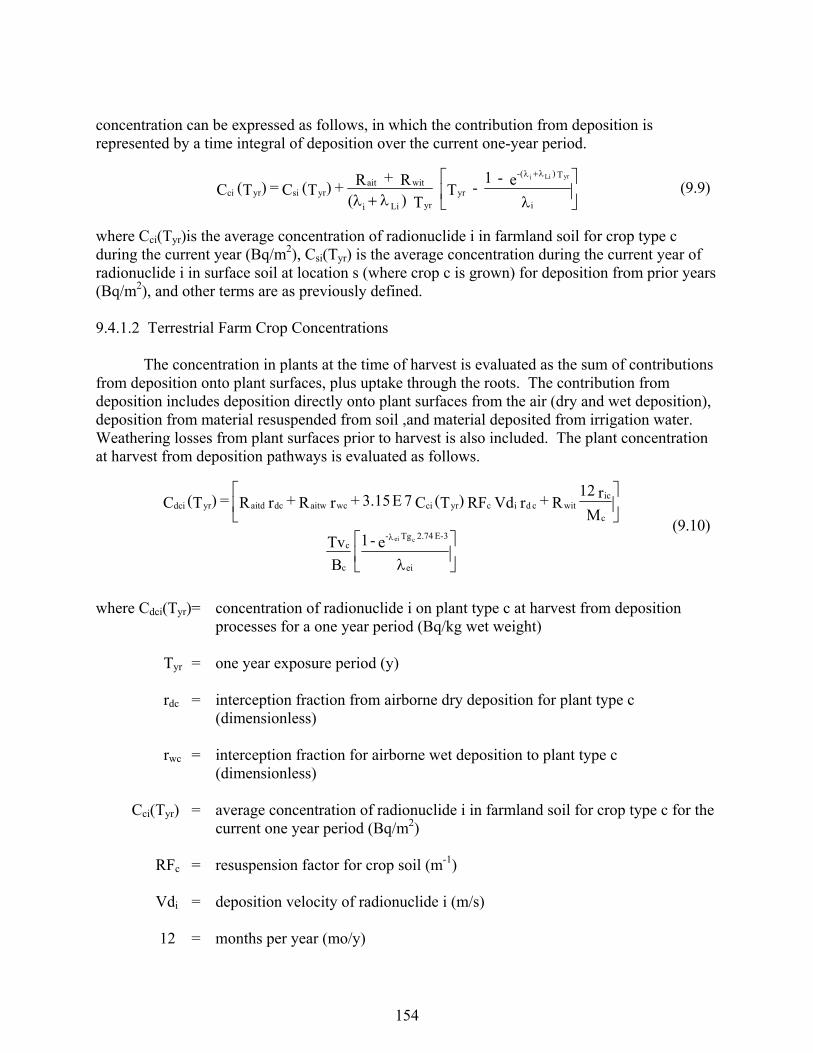
154

concentration can be expressed as follows, in which the contribution from deposition is represented by a time integral of deposition over the current one-year period.

where Cci(Tyr)is the average concentration of radionuclide i in farmland soil for crop type c during the current year (Bq/m2), Csi(Tyr) is the average concentration during the current year of radionuclide i in surface soil at location s (where crop c is grown) for deposition from prior years (Bq/m2), and other terms are as previously defined. 9.4.1.2 Terrestrial Farm Crop Concentrations The concentration in plants at the time of harvest is evaluated as the sum of contributions from deposition onto plant surfaces, plus uptake through the roots. The contribution from deposition includes deposition directly onto plant surfaces from the air (dry and wet deposition), deposition from material resuspended from soil ,and material deposited from irrigation water. Weathering losses from plant surfaces prior to harvest is also included. The plant concentration at harvest from deposition pathways is evaluated as follows.

where Cdci(Tyr)= concentration of radionuclide i on plant type c at harvest from deposition processes for a one year period (Bq/kg wet weight)

Tyr = one year exposure period (y) rdc = interception fraction from airborne dry deposition for plant type c

(dimensionless) rwc = interception fraction for airborne wet deposition to plant type c

(dimensionless) Cci(Tyr) = average concentration of radionuclide i in farmland soil for crop type c for the

current one year period (Bq/m2) RFc = resuspension factor for crop soil (m-1) Vdi = deposition velocity of radionuclide i (m/s) 12 = months per year (mo/y)

i

T ) (-

yryrLii

witaityrsiyrci

e - 1 - T

T )(

R + R + )T( C = )T( CyrLii

(9.9)

ei

3E-2.74 Tg -

c

c

c

icwitcdicyrciwcaitwdcaitdyrdci

e - 1

B

Tv

M

r 12 R + r Vd RF )T(C 7E3.15 + r R + r R = )T(C

cei

(9.10)

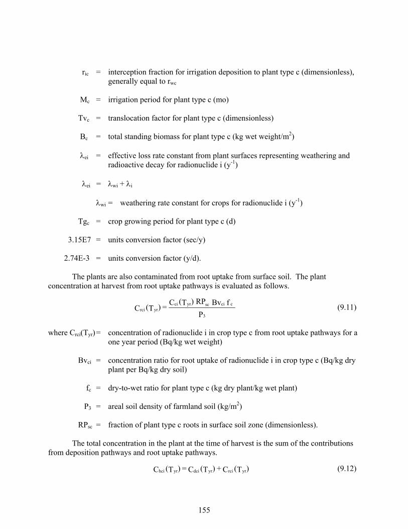
155

ric = interception fraction for irrigation deposition to plant type c (dimensionless),

generally equal to rwc Mc = irrigation period for plant type c (mo) Tvc = translocation factor for plant type c (dimensionless) Bc = total standing biomass for plant type c (kg wet weight/m2) ei = effective loss rate constant from plant surfaces representing weathering and

radioactive decay for radionuclide i (y-1) ei = wi + i wi = weathering rate constant for crops for radionuclide i (y-1) Tgc = crop growing period for plant type c (d) 3.15E7 = units conversion factor (sec/y) 2.74E-3 = units conversion factor (y/d). The plants are also contaminated from root uptake from surface soil. The plant concentration at harvest from root uptake pathways is evaluated as follows.

where Crci(Tyr) = concentration of radionuclide i in crop type c from root uptake pathways for a one year period (Bq/kg wet weight)

Bvci = concentration ratio for root uptake of radionuclide i in crop type c (Bq/kg dry

plant per Bq/kg dry soil) fc = dry-to-wet ratio for plant type c (kg dry plant/kg wet plant) P3 = areal soil density of farmland soil (kg/m2) RPsc = fraction of plant type c roots in surface soil zone (dimensionless). The total concentration in the plant at the time of harvest is the sum of the contributions from deposition pathways and root uptake pathways.

P

fBv RP)T(C = )T(C

3

cciscyrciyrrci (9.11)

)T(C + )T(C = )T(C yrrciyrdciyrhci (9.12)

156

where Chci(Tyr) is the concentration in plant type c at harvest for a one year period (Bq/kg wet weight) and other terms are as previously defined. The concentration in crops at the time of consumption is evaluated by accounting for decay between harvest and consumption. The holdup delay time defines this time period. The calculation is performed using the decay processor (see Appendix C). The calculation is represented for the parent radionuclide as follows.

where Ccsi(Tyr) = concentration of radionuclide i in crop type c at location s at the time of consumption over a one year period (Bq/kg wet weight)

Thc = holdup delay time between harvest and consumption for crop type c (d) i = radiological decay constant for radionuclide i (y-1) 2.74E-3 = conversion factor years day-1. 9.4.1.3 Terrestrial Farm Animal Product Concentrations Pathways by which animal products may become contaminated include animal ingestion of plants, water, and soil (the animals’ inhalation is neglected as contributing little to the total). The concentration in feed plants is evaluated in a similar manner to the food crop calculations as defined in Equations (9.10) through (9.13), with parameters defined for animal feed crops in place of human food crops. The feed crop concentration at the time of animal feeding, Ccfi(Tyr), is evaluated using Equation (9.13) with the holdup delay time representing the time between harvest and consumption by animals. The water concentration is the value supplied on the input file, Cwi(Tyr), as the average concentration over the current year. The soil concentration is the average surface soil concentration for the year given by the parameter, Cai(Tyr), for animal product, a, and radionuclide i in units of Bq/m2, evaluated using Equation (9.9). The concentration in an animal product at the time of harvest (slaughter, milking, or egg collection), is evaluated as follows.

where Chai(Tyr) = concentration of radionuclide i in animal product a at harvest of the animal product for a one year period (Bq/kg)

Tyr = one year exposure period (y)

e )T(C = )T( C 3E-2.74 Th -yrhciyrcsi

ci (9.13)

U d )T(C +U d )T(C + U d )T( C Fa = )T( C afafyrcfi

N

1=fasasyraiawawyrwiiyrhai

af

(9.14)

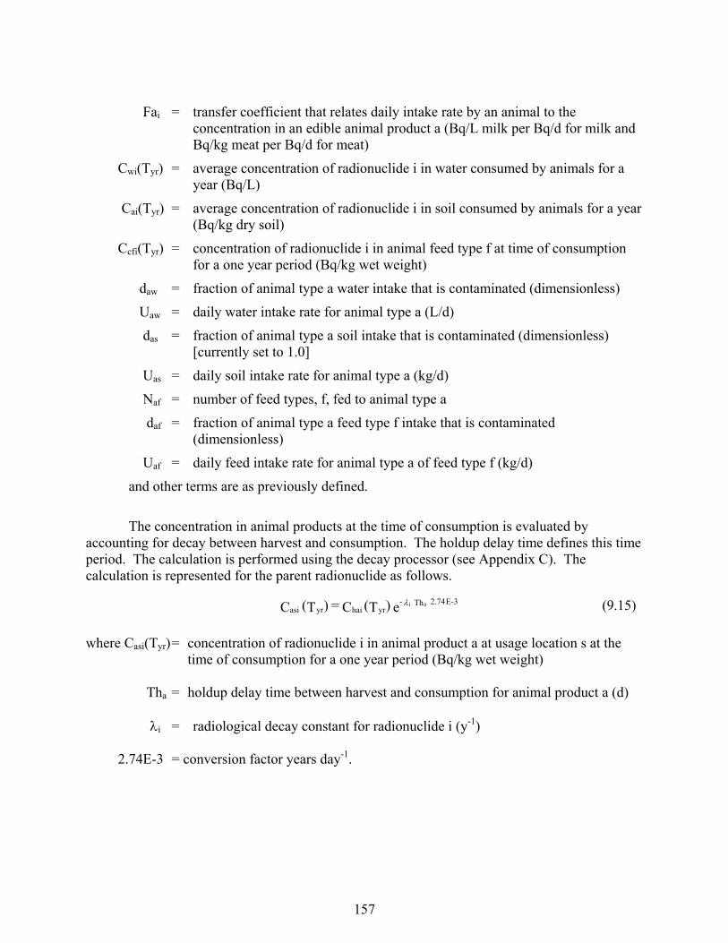
157

Fai = transfer coefficient that relates daily intake rate by an animal to the concentration in an edible animal product a (Bq/L milk per Bq/d for milk and Bq/kg meat per Bq/d for meat)

Cwi(Tyr) = average concentration of radionuclide i in water consumed by animals for a year (Bq/L)

Cai(Tyr) = average concentration of radionuclide i in soil consumed by animals for a year (Bq/kg dry soil)

Ccfi(Tyr) = concentration of radionuclide i in animal feed type f at time of consumption for a one year period (Bq/kg wet weight)

daw = fraction of animal type a water intake that is contaminated (dimensionless)

Uaw = daily water intake rate for animal type a (L/d)

das = fraction of animal type a soil intake that is contaminated (dimensionless) [currently set to 1.0]

Uas = daily soil intake rate for animal type a (kg/d)

Naf = number of feed types, f, fed to animal type a

daf = fraction of animal type a feed type f intake that is contaminated (dimensionless)

Uaf = daily feed intake rate for animal type a of feed type f (kg/d)

and other terms are as previously defined.

The concentration in animal products at the time of consumption is evaluated by accounting for decay between harvest and consumption. The holdup delay time defines this time period. The calculation is performed using the decay processor (see Appendix C). The calculation is represented for the parent radionuclide as follows.

where Casi(Tyr) = concentration of radionuclide i in animal product a at usage location s at the time of consumption for a one year period (Bq/kg wet weight)

Tha = holdup delay time between harvest and consumption for animal product a (d) i = radiological decay constant for radionuclide i (y-1) 2.74E-3 = conversion factor years day-1.

e )T(C = )T( C 3E-2.74 Th -yrhaiyrasi

ai (9.15)

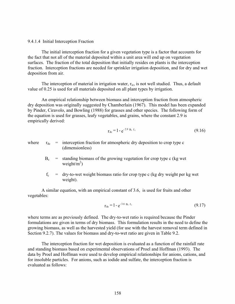
158

9.4.1.4 Initial Interception Fraction The initial interception fraction for a given vegetation type is a factor that accounts for the fact that not all of the material deposited within a unit area will end up on vegetation surfaces. The fraction of the total deposition that initially resides on plants is the interception fraction. Interception fractions are needed for sprinkler irrigation deposition, and for dry and wet deposition from air. The interception of material in irrigation water, ric, is not well studied. Thus, a default value of 0.25 is used for all materials deposited on all plant types by irrigation. An empirical relationship between biomass and interception fraction from atmospheric dry deposition was originally suggested by Chamberlain (1967). This model has been expanded by Pinder, Ciravolo, and Bowling (1988) for grasses and other species. The following form of the equation is used for grasses, leafy vegetables, and grains, where the constant 2.9 is empirically derived:

where rdc = interception fraction for atmospheric dry deposition to crop type c (dimensionless)

Bc = standing biomass of the growing vegetation for crop type c (kg wet

weight/m2) fc = dry-to-wet weight biomass ratio for crop type c (kg dry weight per kg wet

weight). A similar equation, with an empirical constant of 3.6, is used for fruits and other vegetables:

where terms are as previously defined. The dry-to-wet ratio is required because the Pinder formulations are given in terms of dry biomass. This formulation results in the need to define the growing biomass, as well as the harvested yield (for use with the harvest removal term defined in Section 9.2.7). The values for biomass and dry-to-wet ratio are given in Table 9.2. The interception fraction for wet deposition is evaluated as a function of the rainfall rate and standing biomass based on experimental observations of Proel and Hoffman (1993). The data by Proel and Hoffman were used to develop empirical relationships for anions, cations, and for insoluble particles. For anions, such as iodide and sulfate, the interception fraction is evaluated as follows:

e - 1 = r f B 2.9 -dc

cc (9.16)

e - 1 = r f B 3.6 -dc

cc (9.17)

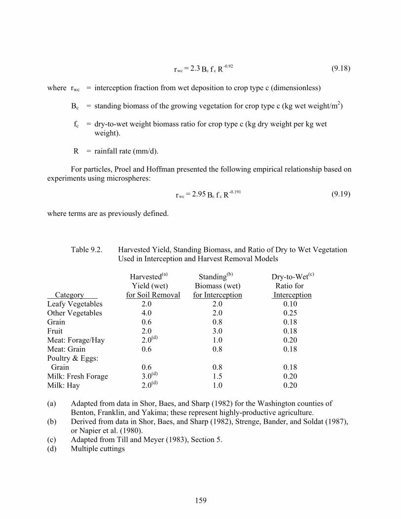
159

where rwc = interception fraction from wet deposition to crop type c (dimensionless) Bc = standing biomass of the growing vegetation for crop type c (kg wet weight/m2) fc = dry-to-wet weight biomass ratio for crop type c (kg dry weight per kg wet

weight). R = rainfall rate (mm/d). For particles, Proel and Hoffman presented the following empirical relationship based on experiments using microspheres:

where terms are as previously defined. Table 9.2. Harvested Yield, Standing Biomass, and Ratio of Dry to Wet Vegetation

Used in Interception and Harvest Removal Models Harvested(a) Standing(b) Dry-to-Wet(c) Yield (wet) Biomass (wet) Ratio for Category for Soil Removal for Interception Interception Leafy Vegetables 2.0 2.0 0.10 Other Vegetables 4.0 2.0 0.25 Grain 0.6 0.8 0.18 Fruit 2.0 3.0 0.18 Meat: Forage/Hay 2.0(d) 1.0 0.20 Meat: Grain 0.6 0.8 0.18 Poultry & Eggs: Grain 0.6 0.8 0.18 Milk: Fresh Forage 3.0(d) 1.5 0.20 Milk: Hay 2.0(d) 1.0 0.20 (a) Adapted from data in Shor, Baes, and Sharp (1982) for the Washington counties of

Benton, Franklin, and Yakima; these represent highly-productive agriculture. (b) Derived from data in Shor, Baes, and Sharp (1982), Strenge, Bander, and Soldat (1987),

or Napier et al. (1980). (c) Adapted from Till and Meyer (1983), Section 5. (d) Multiple cuttings

R f B 2.3 = r -0.92ccwc (9.18)

R f B 2.95 = r -0.191ccwc (9.19)

160

9.4.1.5 Resuspension Factor The resuspension factor relates the radionuclide concentration in soil (per unit area, i.e., m-1) to the concentration in air. The resuspension factor for food crop and animal product pathways is representative of conditions on farmland, which may be different from the resuspension factor for the inhalation exposure pathway. Farmland would be expected to be tilled and have soil generally looser than soil for the general residential exposure situations. 9.4.1.6 Translocation Factor and Weathering Loss Material deposited on plant surfaces is subject to absorption and removal processes. The translocation factor indicates the fraction of total deposition to plant surfaces that is incorporated into edible parts of the plant. A value of 1 is assumed for leafy vegetables and forage crops, and 0.1 for all other vegetation. Losses from plant surfaces are represented by a weathering rate constant, wi. The rate constant is based on a weathering half time of 14 days (as used by many sources; originally derived by Soldat et al. 1974). 9.4.2 Aquatic Food Ingestion Aquatic food products may become contaminated when grown in contaminated surface waters. The aquatic food pathways include ingestion of fish, crustaceans, mollusks, and aquatic plants. The concentration in an aquatic food is based on the average surface water concentration for the current year, as follows.

where Chqi(Tyr)= concentration of radionuclide i in aquatic food type q at time of harvest (Bq/kg)

Bqi = bioaccumulation factor for radionuclide i in the edible portions of aquatic food

type q (Bq/kg wet fish per Bq/L water). The concentration at the start of the consumption period is evaluated accounting for decay during holdup as follows:

where Cfwi(Tyr)= concentration of radionuclide i in aquatic food type q at water location w the time of consumption (Bq/kg wet weight)

Thq = holdup delay time between harvest and consumption for aquatic food type q

(d)

B )T(C = )T(C qiyrwiyrhqi (9.20)

e )T(C = )T( C 3E-2.74 Th -yrihqyrwif

qi (9.21)

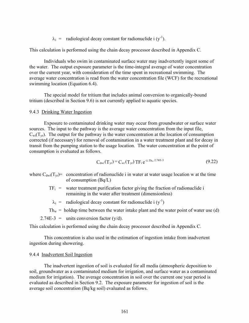
161

i = radiological decay constant for radionuclide i (y-1). This calculation is performed using the chain decay processor described in Appendix C. Individuals who swim in contaminated surface water may inadvertently ingest some of the water. The output exposure parameter is the time-integral average of water concentration over the current year, with consideration of the time spent in recreational swimming. The average water concentration is read from the water concentration file (WCF) for the recreational swimming location (Equation 6.4). The special model for tritium that includes animal conversion to organically-bound tritium (described in Section 9.6) is not currently applied to aquatic species. 9.4.3 Drinking Water Ingestion Exposure to contaminated drinking water may occur from groundwater or surface water sources. The input to the pathway is the average water concentration from the input file, Cwi(Tyr). The output for the pathway is the water concentration at the location of consumption corrected (if necessary) for removal of contamination in a water treatment plant and for decay in transit from the pumping station to the usage location. The water concentration at the point of consumption is evaluated as follows.

where Cdwi(Tyr)= concentration of radionuclide i in water at water usage location w at the time of consumption (Bq/L)

TFi = water treatment purification factor giving the fraction of radionuclide i remaining in the water after treatment (dimensionless)

i = radiological decay constant for radionuclide i (y-1)

Thw = holdup time between the water intake plant and the water point of water use (d)

2.74E-3 = units conversion factor (y/d).

This calculation is performed using the chain decay processor described in Appendix C. This concentration is also used in the estimation of ingestion intake from inadvertent ingestion during showering. 9.4.4 Inadvertent Soil Ingestion The inadvertent ingestion of soil is evaluated for all media (atmospheric deposition to soil, groundwater as a contaminated medium for irrigation, and surface water as a contaminated medium for irrigation). The average concentration in soil over the current one year period is evaluated as described in Section 9.2. The exposure parameter for ingestion of soil is the average soil concentration (Bq/kg soil) evaluated as follows.

e TF )T(C = )T(C 3E-2.74 Th -iyrwiyrdwi

wi (9.22)

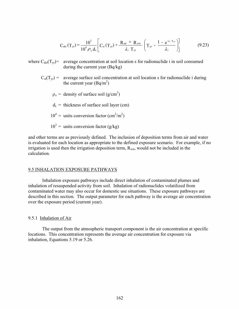
162

where Cdsi(Tyr) = average concentration at soil location s for radionuclide i in soil consumed during the current year (Bq/kg)

Csi(Tyr) = average surface soil concentration at soil location s for radionuclide i during

the current year (Bq/m2) s = density of surface soil (g/cm3) ds = thickness of surface soil layer (cm) 104 = units conversion factor (cm2/m2) 103 = units conversion factor (g/kg) and other terms are as previously defined. The inclusion of deposition terms from air and water is evaluated for each location as appropriate to the defined exposure scenario. For example, if no irrigation is used then the irrigation deposition term, Rwit, would not be included in the calculation. 9.5 INHALATION EXPOSURE PATHWAYS Inhalation exposure pathways include direct inhalation of contaminated plumes and inhalation of resuspended activity from soil. Inhalation of radionuclides volatilized from contaminated water may also occur for domestic use situations. These exposure pathways are described in this section. The output parameter for each pathway is the average air concentration over the exposure period (current year). 9.5.1 Inhalation of Air The output from the atmospheric transport component is the air concentration at specific locations. This concentration represents the average air concentration for exposure via inhalation, Equations 5.19 or 5.26.

i

T -

yryri

witaityrsi

ss4

3

yrdsie - 1

- T T

R + R + )T( C d 10

10 = )T( Cyri

(9.23)

163

9.5.2 Inhalation of Resuspended Soil The model for inhalation exposure from resuspended activity uses the resuspension factor approach (as described in Section 9.4.1.2). The resuspension factor relates the soil concentration (per unit area) to the air concentration (per unit volume) and has units of m-1. The use of resuspension factors is based on the assumption that the particulate matter in the air has the same activity as the soil at the location. This is represented mathematically as follows.

where Csai(Tyr) = air concentration of radionuclide i at soil resuspension exposure location a for a year (Bq/m3)

RFa = resuspension factor for soil exposure locations (m-1) Csi(Tyr) = average surface soil concentration over the current year at the soil exposure

location s from material deposited in prior years (Bq/m2) and other terms are as previously defined. The inclusion of deposition terms from air and water is evaluated for each location as appropriate to the defined exposure scenario. For example, if no waterborne deposition is present, then the waterborne deposition term, Rwit, would not be included in the calculation. The resuspension factor may be estimated in one of two ways - either by using a time-dependent function developed by Anspaugh et al. (1975) or by means of a mass loading factor. The Anspaugh resuspension factor is given as follows.

where 10-4 = resuspension factor at the time of initial deposition to soil (m-1) t = time after initial deposition of material to soil (d) 0.15 = effective decay constant controlling the availability of material for resuspension

(d1/2) 10-9 = resuspension factor after 17 years (m-1). The second term in this equation is added based on the assumption that no further measurable decrease in the resuspension factor process occurs after about 17 years, the longest period for which there are data available. In the implementation, an assumption is made that only the top thin layer of soil is available for resuspension using the Anspaugh method.

i

T )(-

yryrLii

witaityrsiayrsai

e - 1 - T

T )(

R + R + )T( C RF = )T( CyrLii

(9.24)

10 + e 10 = RF 9 -t 0.15 -4 -a (9.25)

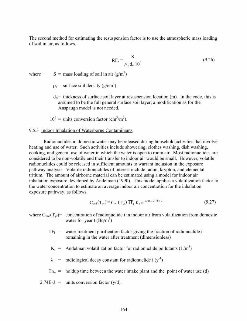
164

The second method for estimating the resuspension factor is to use the atmospheric mass loading of soil in air, as follows.

where S = mass loading of soil in air (g/m3) s = surface soil density (g/cm3). drs = thickness of surface soil layer at resuspension location (m). In the code, this is

assumed to be the full general surface soil layer; a modification as for the Anspaugh model is not needed.

106 = units conversion factor (cm3/m3). 9.5.3 Indoor Inhalation of Waterborne Contaminants Radionuclides in domestic water may be released during household activities that involve heating and use of water. Such activities include showering, clothes washing, dish washing, cooking, and general use of water in which the water is open to room air. Most radionuclides are considered to be non-volatile and their transfer to indoor air would be small. However, volatile radionuclides could be released in sufficient amounts to warrant inclusion in the exposure pathway analysis. Volatile radionuclides of interest include radon, krypton, and elemental tritium. The amount of airborne material can be estimated using a model for indoor air inhalation exposure developed by Andelman (1990). This model applies a volatilization factor to the water concentration to estimate an average indoor air concentration for the inhalation exposure pathway, as follows.

where Cvwi(Tyr)= concentration of radionuclide i in indoor air from volatilization from domestic water for year t (Bq/m3)

TFi = water treatment purification factor giving the fraction of radionuclide i

remaining in the water after treatment (dimensionless) Kr = Andelman volatilization factor for radionuclide pollutants (L/m3) i = radiological decay constant for radionuclide i (y-1) Thw = holdup time between the water intake plant and the point of water use (d) 2.74E-3 = units conversion factor (y/d).

10 d

S = RF 6

rss

a (9.26)

e K TF )T(C = )T(C 3E-2.74 Th -riyrwiyr

wivwi (9.27)

165

The numerical value suggested for the volatilization factor is 0.1 L/m3 for 222Rn. This value could reasonably be used for other noble gases and elemental tritium. For other radionuclides, significant volatilization is not expected. An exception would be if the radionuclide were associated with a volatile chemical (as for a tagged tracer chemical). In this case the volatilization factor of 0.5 may be appropriate, as suggested by Andelman for volatile chemicals. A minimum value for the volatilization factor can be estimated from a recent study on the behavior of hexavalent chromium in tapwater (Finley et al. 1996). Measurements of the airborne concentration of chromium were made within a shower stall in which contaminated water was sprayed against a mannequin. The results indicated that the air concentration of chromium could be approximated by multiplying by a factor of 3.0x10-5, with concentration units as expressed for Equation (9.33). This suggests that a minimum value to use in place of the Andelman volatilization factor would be 3.0x10-5 (L/m3) for non-volatile radionuclides. Indoor air is assumed to contain contaminants that have infiltrated from outdoors. The value calculated for Cvwi(Tyr) is then added to the outdoor air concentration calculated using Equations 5.19 or 5.28 to give the total indoor air concentration. 9.6 SPECIAL RADIONUCLIDE MODELS: TRITIUM AND CARBON-14 The behavior of the radionuclides tritium and carbon-14 in exposure pathways is handled in a special manner. The concentrations of tritium or carbon-14 in environmental media (soil, plants, and animal products) are assumed to be related to the specific activity (Becquerels of radionuclide per kilogram of soluble element) in the contaminating medium (air or water). The fractional content of hydrogen or carbon in a plant or animal product is then used to compute the concentration of tritium or carbon-14 in the food product under consideration. The hydrogen contents in both the water and the nonwater (dry) portion of the food product are used when calculating the tritium concentration. The creation of organically-bound tritium in plant and animal products from intake of HTO is also addressed. For airborne releases, it is assumed that plants obtain all their carbon from airborne carbon dioxide and that animals obtain all their carbon through ingestion of plants. The transfer of 14C from water to plants is difficult to model because plants acquire most of their carbon from the air. Currently available models for 14C uptake by plants from water use specific-activity models relating the activity in the plants directly to the activity in irrigation water. This is extremely conservative in that it assumes that plants receive all of their carbon from water. The model described here is based on the ratio of grams of carbon-14 to grams of total carbon in soil and a correction for the amount of carbon plants obtain from soil. The special models for 3H as water vapor (HTO) and elemental tritium gas (HT) are described first. The models implemented in GENII are a variant of the model proposed by Peterson and Davis (2002), the primary difference relates to uptake of tritiated drinking water by farm animals (in GENII, this is controlled by input water concentrations, not atmospheric conditions). The 14C models are then described.

166

9.6.1 Special Tritium Models Tritiated Water (HTO)

For HTO releases, concentrations in air moisture Cam (Bq L-1) are found by dividing the concentration in air (Bq m-3) by the absolute humidity (kg or L m-3).

To estimate HTO concentrations in plant products, it is assumed conservatively that the concentration of HTO in plant water equals 0.9 Cam for leafy vegetables and pasture and 0.8 Cam for fruit, root crops and other vegetables, and grain. These reduction factors account for dilution from soil water, which has a lower tritium concentration than does air moisture for atmospheric releases and which affects fruit and root crops more than leaves (Table 9.3). OBT concentrations in plants are estimated from a plant water concentration of 0.9 Cam for all plant types, since OBT is assumed to form exclusively in the leaves and to be translocated to other plant parts. Then, isotopic discrimination occurring in the formation of OBT (Table 9.4) is assumed conservatively to result in an OBT concentration 0.9 times the concentration of HTO in plant water.

The equation for calculating concentrations of HTO in plant products (Bq kg-1 fw) is:

Cpp_HTO = RFpp Cam Ffw_pp (9.28)

where RFpp = reduction factor that accounts for low soil water concentrations relative to

concentrations in air moisture and varies by vegetable type The equation for calculating concentrations of OBT in plant products (Bq kg-1 fw) is:

Cpp_OBT = RFl IDpp Cam Fdm_pp Weq_pp (9.29) where RFl = reduction factor for plant leaves IDpp = isotopic discrimination factor for plant products Values and definitions for the parameters appearing in Eqns (9.28) and (9.29) for leafy vegetables, fruit, root and other vegetables, grain and pasture are shown in Table 9.3. Values for fresh and dry matter fractions and water equivalent factors were obtained from Geigy (1981).

HTO concentrations in animals are assumed to equal the weighted average tritium concentration of ingested water based on the fraction of water supplied by each source. These sources comprise food (from plant water and digested organically bound molecules) and drinking water. The concentration of tritium in animal products is calculated from the concentrations in feed and water, as follows.

167

)UWFU F( + U

d U )T(C + d U )T(C F = )T(C

afpp_eqpp_dmafpp_fw

N

1=fwa

afafyrcfH

N

1=fawwayrwH

ap_fwyrHTOapfa

fa

(9.30a)

where CHTOap(Tyr) = concentration of tritiated water in animal product a at time of consumption by humans over a one year period (Bq/kg)

Ffw_ap = fraction of water in animal product a (dimensionless) CwH(Tyr) = average concentration of tritium i in water consumed by animal type a

over a one year period (Bq/L) Uwa = daily water intake rate for animal type a (L/d) daw = fraction of animal type a water intake that is contaminated (dimensionless) CcfH(Tyr) = concentration of tritium (the sum of the water and organic portions,

estimated as described above) in animal feed type f at time of consumption for a one year period (Bq/kg wet weight)

Uaf = daily intake rate for animal type a of feed type f (kg/d) daf = fraction of animal type a feed type f intake that is contaminated

(dimensionless) Nfa = number of feed crops eaten by animal type a and the other constants are as previously defined. The concentration of tritium in animal feed is evaluated using Equations (9.28) and (9.29) with values defined for the animal feed crops.

The equation to calculate OBT in animal products assumes the specific activity in organic material equals the specific activity in the aqueous phase apart from a discrimination factor. This equation is adapted from the derivation of Peterson and Davis (2002).

Cap_OBT = Cap_HTO Fdm_apWeq_ap / Ffw_ap (9.30b) Default values for parameters in eqns (9.30a) and (9.30b), as recommended by Peterson and Davis (2002), are presented in Table 9.4. Values for fresh and dry matter fractions and for water equivalent factors are from Geigy (1981).

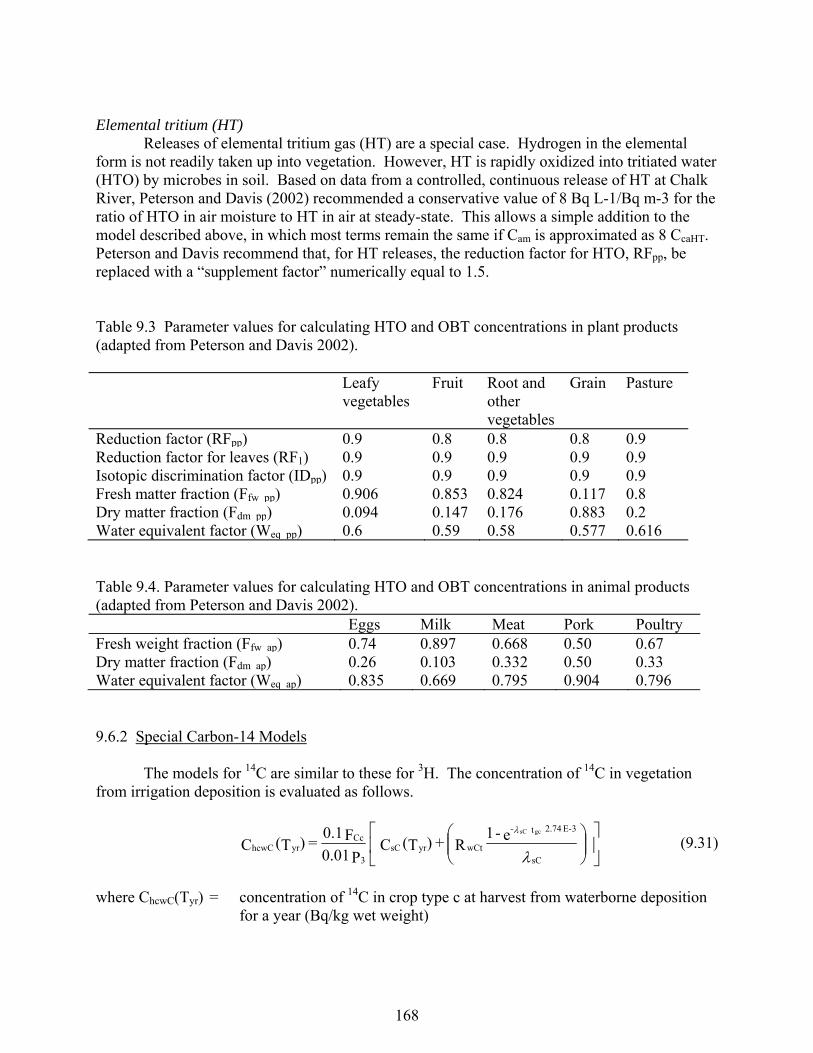
168

Elemental tritium (HT) Releases of elemental tritium gas (HT) are a special case. Hydrogen in the elemental form is not readily taken up into vegetation. However, HT is rapidly oxidized into tritiated water (HTO) by microbes in soil. Based on data from a controlled, continuous release of HT at Chalk River, Peterson and Davis (2002) recommended a conservative value of 8 Bq L-1/Bq m-3 for the ratio of HTO in air moisture to HT in air at steady-state. This allows a simple addition to the model described above, in which most terms remain the same if Cam is approximated as 8 CcaHT. Peterson and Davis recommend that, for HT releases, the reduction factor for HTO, RFpp, be replaced with a “supplement factor” numerically equal to 1.5. Table 9.3 Parameter values for calculating HTO and OBT concentrations in plant products (adapted from Peterson and Davis 2002). Leafy

vegetables Fruit Root and

other vegetables

Grain Pasture

Reduction factor (RFpp) 0.9 0.8 0.8 0.8 0.9 Reduction factor for leaves (RF1) 0.9 0.9 0.9 0.9 0.9 Isotopic discrimination factor (IDpp) 0.9 0.9 0.9 0.9 0.9 Fresh matter fraction (Ffw pp) 0.906 0.853 0.824 0.117 0.8 Dry matter fraction (Fdm pp) 0.094 0.147 0.176 0.883 0.2 Water equivalent factor (Weq pp) 0.6 0.59 0.58 0.577 0.616 Table 9.4. Parameter values for calculating HTO and OBT concentrations in animal products (adapted from Peterson and Davis 2002). Eggs Milk Meat Pork Poultry Fresh weight fraction (Ffw ap) 0.74 0.897 0.668 0.50 0.67 Dry matter fraction (Fdm ap) 0.26 0.103 0.332 0.50 0.33 Water equivalent factor (Weq ap) 0.835 0.669 0.795 0.904 0.796 9.6.2 Special Carbon-14 Models The models for 14C are similar to these for 3H. The concentration of 14C in vegetation from irrigation deposition is evaluated as follows.

e - 1

R + )T(C P 0.01

F 0.1 = )T(C

sC

3E-2.74 t -

wCtyrsC3

CcyrhcwC

gcsC

(9.31)

where ChcwC(Tyr) = concentration of 14C in crop type c at harvest from waterborne deposition

for a year (Bq/kg wet weight)

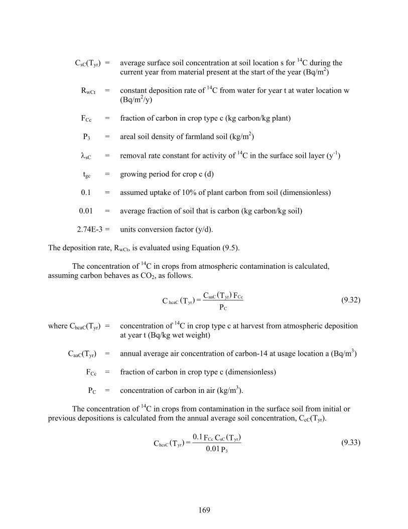
169

CsC(Tyr) = average surface soil concentration at soil location s for 14C during the current year from material present at the start of the year (Bq/m2)

RwCt = constant deposition rate of 14C from water for year t at water location w

(Bq/m2/y) FCc = fraction of carbon in crop type c (kg carbon/kg plant) P3 = areal soil density of farmland soil (kg/m2) sC = removal rate constant for activity of 14C in the surface soil layer (y-1) tgc = growing period for crop c (d) 0.1 = assumed uptake of 10% of plant carbon from soil (dimensionless) 0.01 = average fraction of soil that is carbon (kg carbon/kg soil) 2.74E-3 = units conversion factor (y/d). The deposition rate, RwCt, is evaluated using Equation (9.5). The concentration of 14C in crops from atmospheric contamination is calculated, assuming carbon behaves as CO2, as follows.

P

F )T(C = )T( C

C

CcyraaCyrhcaC (9.32)

where ChcaC(Tyr) = concentration of 14C in crop type c at harvest from atmospheric deposition

at year t (Bq/kg wet weight) CaaC(Tyr) = annual average air concentration of carbon-14 at usage location a (Bq/m3) FCc = fraction of carbon in crop type c (dimensionless) PC = concentration of carbon in air (kg/m3). The concentration of 14C in crops from contamination in the surface soil from initial or previous depositions is calculated from the annual average soil concentration, CcC(Tyr).

P 0.01

)T(C F 0.1 = )T(C

3

yrsCCcyrhcsC (9.33)

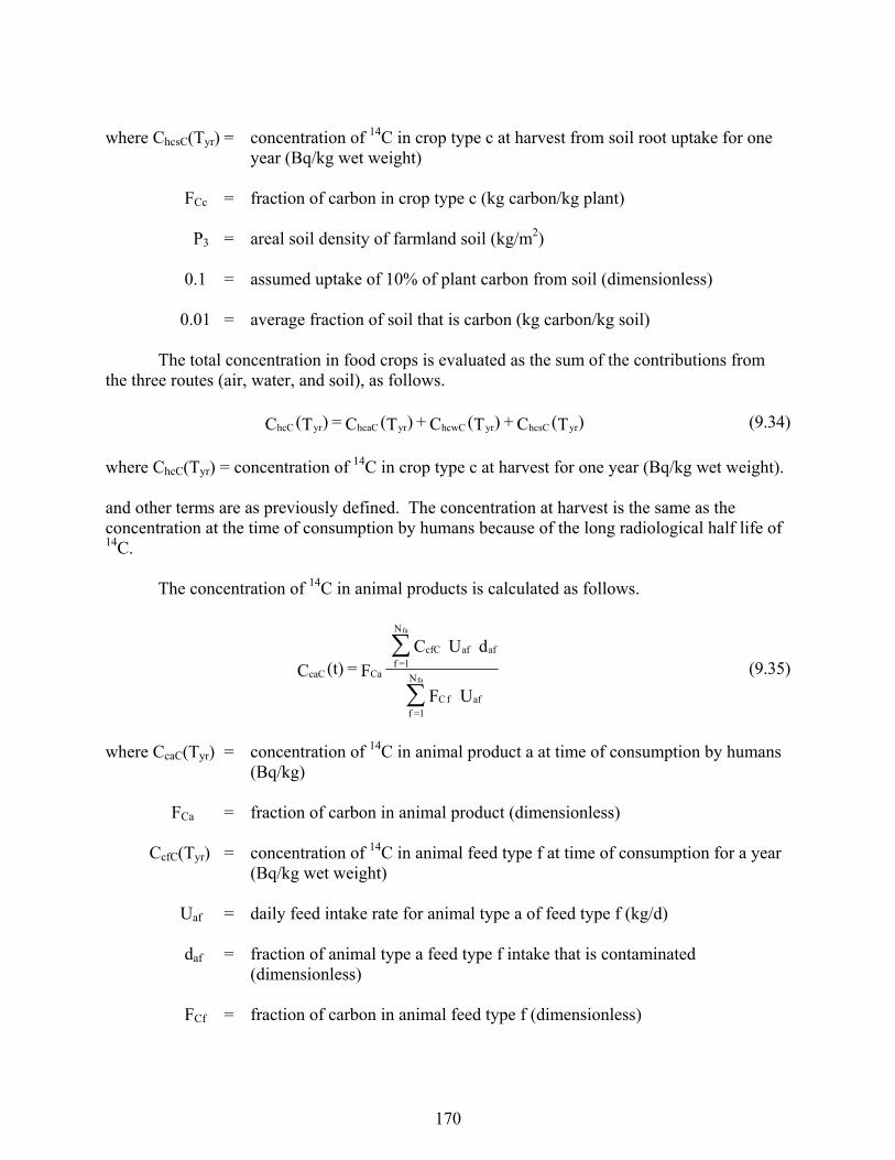
170

where ChcsC(Tyr) = concentration of 14C in crop type c at harvest from soil root uptake for one year (Bq/kg wet weight)

FCc = fraction of carbon in crop type c (kg carbon/kg plant) P3 = areal soil density of farmland soil (kg/m2) 0.1 = assumed uptake of 10% of plant carbon from soil (dimensionless) 0.01 = average fraction of soil that is carbon (kg carbon/kg soil) The total concentration in food crops is evaluated as the sum of the contributions from the three routes (air, water, and soil), as follows.

)T(C + )T(C + )T(C = )T(C yrhcsCyrhcwCyrhcaCyrhcC (9.34)

where ChcC(Tyr) = concentration of 14C in crop type c at harvest for one year (Bq/kg wet weight). and other terms are as previously defined. The concentration at harvest is the same as the concentration at the time of consumption by humans because of the long radiological half life of 14C. The concentration of 14C in animal products is calculated as follows.

U F

d U C

F = (t)C

affC

N

1=f

afafcfC

N

1=fCacaC

fa

fa

(9.35)

where CcaC(Tyr) = concentration of 14C in animal product a at time of consumption by humans

(Bq/kg) FCa = fraction of carbon in animal product (dimensionless) CcfC(Tyr) = concentration of 14C in animal feed type f at time of consumption for a year

(Bq/kg wet weight) Uaf = daily feed intake rate for animal type a of feed type f (kg/d) daf = fraction of animal type a feed type f intake that is contaminated

(dimensionless) FCf = fraction of carbon in animal feed type f (dimensionless)

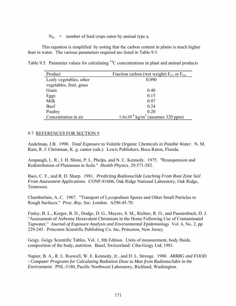
171

Nfa = number of feed crops eaten by animal type a. This equation is simplified by noting that the carbon content in plants is much higher than in water. The various parameters required are listed in Table 9.5. Table 9.5. Parameter values for calculating 14C concentrations in plant and animal products

Product Fraction carbon (wet weight) FCc or FCa Leafy vegetables, other vegetables, fruit, grass

0.090

Grain 0.40 Eggs 0.15 Milk 0.07 Beef 0.24 Poultry 0.20 Concentration in air 1.6x10-4 kg/m3 (assumes 320 ppm)

9.7 REFERENCES FOR SECTION 9 Andelman, J.B. 1990. Total Exposure to Volatile Organic Chemicals in Potable Water. N. M. Ram, R. f. Christman, K. g. cantor (eds.). Lewis Publishers, Boca Raton, Florida. Anspaugh, L. R., J. H. Shinn, P. L. Phelps, and N. C. Kennedy. 1975. "Resuspension and Redistribution of Plutonium in Soils." Health Physics. 29:571-582. Baes, C. F., and R. D. Sharp. 1981. Predicting Radionuclide Leaching From Root Zone Soil From Assessment Applications. CONF-81606, Oak Ridge National Laboratory, Oak Ridge, Tennessee. Chamberlain, A. C. 1967. "Transport of Lycopodium Spores and Other Small Particles to Rough Surfaces." Proc. Roy. Soc. London. A296:45-70. Finley, B. L., Kerger, B. D., Dodge, D. G., Meyers, S. M., Richter, R. O., and Paustenbach, D. J. “Assessment of Airborne Hexavalent Chromium in the Home Following Use of Contaminated Tapwater,” Journal of Exposure Analysis and Environmental Epidemiology Vol. 6, No. 2, pp 229-245. Princeton Scientific Publishing Co. Inc, Princeton, New Jersey. Geigy. Geigy Scientific Tables, Vol. 1, 8th Edition. Units of measurement, body fluids, composition of the body, nutrition. Basel, Switzerland: Ciba-Geigy Ltd; 1981. Napier, B. A., R. L. Roswell, W. E. Kennedy, Jr., and D. L. Strenge. 1980. ARRRG and FOOD - Computer Programs for Calculating Radiation Dose to Man from Radionuclides in the Environment. PNL-3180, Pacific Northwest Laboratory, Richland, Washington.

172

Nelson, J. L. 1965. "Distribution of Sediments and Associated Radionuclides in the Columbia River Below Hanford." In Hanford Radiological Sciences Research and Development Report for 1964, ed. D. W. Reece and J. K. Green, p. 3.80. USAEC Report BNWL-36, Pacific Northwest Laboratory, Richland, Washington. Peterson, S.-R., and P.A. Davis. 2002. “Tritium Doses from Chronic Atmospheric Releases: A New Method Proposed for Regulatory Compliance,” Health Physics, 82(2):213-225. Pinder III, J. E., T. G. Ciravolo, and J. W. Bowling. 1988. "The Interrelationships Among Plant Biomass, Plant Surface Area, and the Interception of Particulate Deposition by Grasses." Health Phys. 55:51-58. Proel, G., and F.O. Hoffman. 1993. The Interception, Initial and Post Deposition-Retention by Vegetation of Dry and Wet Deposited Radionuclides. VAMP Terrestrial Working Group, International Atomic Energy Agency, Vienna, Austria. Shor, R. W., C. F. Baes III, and R. D. Sharp. 1982. Agricultural Production in the United States by County: A Compilation of Information from the 1974 Census of Agriculture for Use in Terrestrial Food Chain Transport and Assessment Models. ORNL-5768. Oak Ridge National Laboratory, Oak Ridge, Tennessee. Soldat, J. K., N. M. Robinson and D. A. Baker. 1974. Models and Computer Codes for Evaluating Environmental Radiation Doses. BNWL-1754. Battelle, Pacific Northwest Laboratory, Richland, Washington. Strenge, D. L., T. J. Bander, and J. K. Soldat. 1987. GASPAR II - Technical Reference and User Guide. NUREG/CR-4653, U.S. Nuclear Regulatory Commis-sion, Washington, D.C. Till, J. E., and H. R. Meyer. 1983. Radiological Assessment - A Textbook on Environmental Dose Analysis. NUREG/CR-3332, U.S Nuclear Regulatory Commission, Washington, D.C. Toombs, G. L., and P. B. Cutler, eds. 1968. Comprehensive Final Report for the Lower Columbia River Environmental Survey in Oregon, June 5, 1961 - July 31, 1967. Oregon State Board of Health, Division of Sanitation and Engineering, Salem, Oregon.

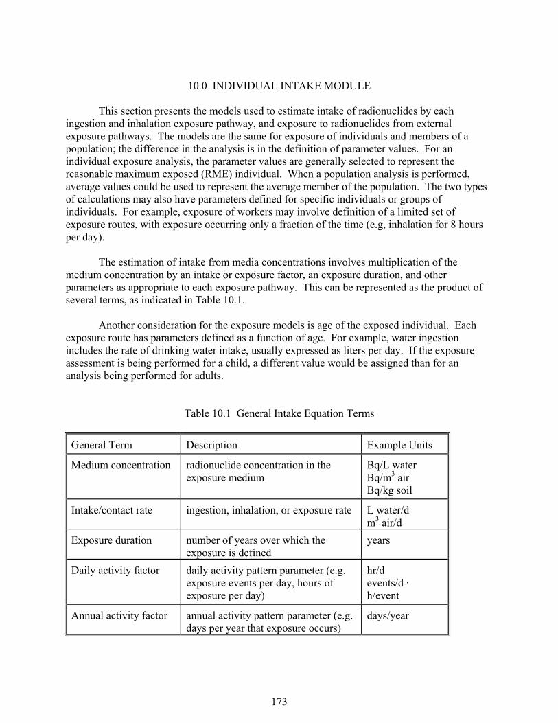
173

10.0 INDIVIDUAL INTAKE MODULE This section presents the models used to estimate intake of radionuclides by each ingestion and inhalation exposure pathway, and exposure to radionuclides from external exposure pathways. The models are the same for exposure of individuals and members of a population; the difference in the analysis is in the definition of parameter values. For an individual exposure analysis, the parameter values are generally selected to represent the reasonable maximum exposed (RME) individual. When a population analysis is performed, average values could be used to represent the average member of the population. The two types of calculations may also have parameters defined for specific individuals or groups of individuals. For example, exposure of workers may involve definition of a limited set of exposure routes, with exposure occurring only a fraction of the time (e.g, inhalation for 8 hours per day). The estimation of intake from media concentrations involves multiplication of the medium concentration by an intake or exposure factor, an exposure duration, and other parameters as appropriate to each exposure pathway. This can be represented as the product of several terms, as indicated in Table 10.1. Another consideration for the exposure models is age of the exposed individual. Each exposure route has parameters defined as a function of age. For example, water ingestion includes the rate of drinking water intake, usually expressed as liters per day. If the exposure assessment is being performed for a child, a different value would be assigned than for an analysis being performed for adults. Table 10.1 General Intake Equation Terms

General Term Description Example Units

Medium concentration radionuclide concentration in the exposure medium

Bq/L water Bq/m3 air Bq/kg soil

Intake/contact rate ingestion, inhalation, or exposure rate L water/d m3 air/d

Exposure duration number of years over which the exposure is defined

years

Daily activity factor daily activity pattern parameter (e.g. exposure events per day, hours of exposure per day)

hr/d events/d · h/event

Annual activity factor annual activity pattern parameter (e.g. days per year that exposure occurs)

days/year

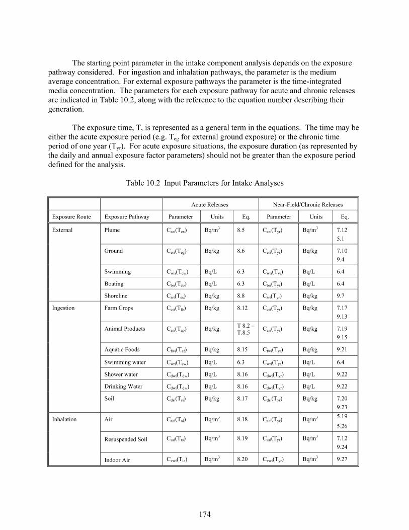
174

The starting point parameter in the intake component analysis depends on the exposure pathway considered. For ingestion and inhalation pathways, the parameter is the medium average concentration. For external exposure pathways the parameter is the time-integrated media concentration. The parameters for each exposure pathway for acute and chronic releases are indicated in Table 10.2, along with the reference to the equation number describing their generation. The exposure time, T, is represented as a general term in the equations. The time may be either the acute exposure period (e.g. Teg for external ground exposure) or the chronic time period of one year (Tyr). For acute exposure situations, the exposure duration (as represented by the daily and annual exposure factor parameters) should not be greater than the exposure period defined for the analysis. Table 10.2 Input Parameters for Intake Analyses

Acute Releases Near-Field/Chronic Releases

Exposure Route Exposure Pathway Parameter Units Eq. Parameter Units Eq.

External Plume Ceai(Tex) Bq/m3 8.5 Ceai(Tyr) Bq/m3 7.12

5.1

Ground Cesi(Teg) Bq/kg 8.6 Cesi(Tyr) Bq/kg 7.10

9.4

Swimming Cwri(Tew) Bq/L 6.3 Cwri(Tyr) Bq/L 6.4

Boating Cbri(Teb) Bq/L 6.3 Cbri(Tyr) Bq/L 6.4

Shoreline Csri(Tes) Bq/kg 8.8 Csri(Tyr) Bq/kg 9.7

Ingestion Farm Crops Ccsi(Tfc) Bq/kg 8.12 Ccsi(Tyr) Bq/kg 7.17

9.13

Animal Products Casi(Tap) Bq/kg T 8.2 – T.8.5

Casi(Tyr) Bq/kg 7.19

9.15

Aquatic Foods Cfwi(Taf) Bq/kg 8.15 Cfwi(Tyr) Bq/kg 9.21

Swimming water Cwri(Tew) Bq/L 6.3 Cwri(Tyr) Bq/L 6.4

Shower water Cdwi(Tdw) Bq/L 8.16 Cdwi(Tyr) Bq/L 9.22

Drinking Water Cdwi(Tdw) Bq/L 8.16 Cdwi(Tyr) Bq/L 9.22

Soil Cdsi(Tsi) Bq/kg 8.17 Cdsi(Tyr) Bq/kg 7.20

9.23

Inhalation Air Caai(Tai) Bq/m3 8.18 Caai(Tyr) Bq/m3 5.19

5.26

Resuspended Soil Csai(Trs) Bq/m3 8.19 Csai(Tyr) Bq/m3 7.12

9.24

Indoor Air Cvwi(Tia) Bq/m3 8.20 Cvwi(Tyr) Bq/m3 9.27

175

10.1 COMMUNICATION INTERFACES The input files for the individual intake module are the global input data file (GID) and the exposure pathway media concentration output file (EPF). No auxiliary data communication files are needed. The exposure pathway media concentration output file (EPF) is generated by the near-field, acute, or chronic exposure modules (or other external program that is capable of generating the proper file information). The GID file section for the individual intake module is generated by the user interface program. It contains information describing the scope of the analysis and all user-provided input parameters for an analysis. The structure and content of the files are given in Appendix A. The output from the individual intake module is the annualized intake of contaminants from various media to which individuals or populations are exposed. For some pathways (those with dose rates associated rather than intakes), the dose rate information is passed instead, modified by the fraction of the time the individual was in the dose field. This information is provided in a primary data communication file, the receptor intake output file (RIF). 10.2 EXTERNAL EXPOSURE ESTIMATES The time-average exposure parameter from the exposure component is used to determine the corresponding time-averaged exposure parameter for the intake component. The latter parameter includes consideration of daily and annual individual activity patterns, and includes dependence on age of the exposed individual. This parameter and the total exposure time (1 year for chronic exposures and the time of plume passage for acute exposures) are carried forward to the Health Risk calculation in Section 11. 10.2.1 External Plume Immersion The evaluation of the plume-immersion intake external-exposure parameter is performed as follows:

where Ieaig = average exposure factor for external plume immersion exposure for radionuclide i for an individual in age group g (Bq/m3)

Ceai = average air concentration at the location of the exposed individual for

radionuclide i (Bq/m3) Ueag = daily exposure factor giving hours of plume immersion exposure per day for

individuals in age group g (h/d) TCp = time correction set equal to Teag/(8760 h/y) for chronic releases and, for acute

releases, (1 d / Ueag ) if Tex is less than Ueag; (1 d / (Tex * (8760 h/y)) if Tex is

pg a e i a e g i a e TC U (T)C = (T)I (10.1)

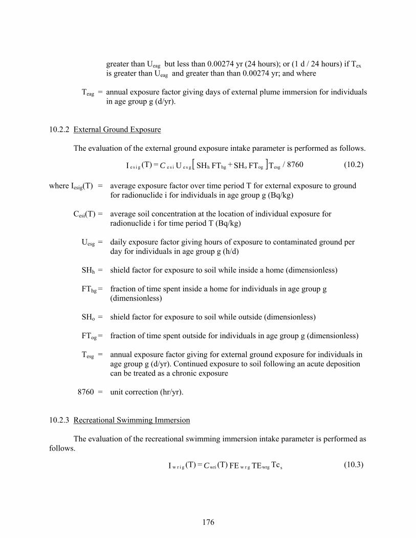
176

greater than Ueag but less than 0.00274 yr (24 hours); or (1 d / 24 hours) if Tex is greater than Ueag and greater than than 0.00274 yr; and where

Teag = annual exposure factor giving days of external plume immersion for individuals

in age group g (d/yr). 10.2.2 External Ground Exposure The evaluation of the external ground exposure intake parameter is performed as follows.

where Iesig(T) = average exposure factor over time period T for external exposure to ground for radionuclide i for individuals in age group g (Bq/kg)

Cesi(T) = average soil concentration at the location of individual exposure for

radionuclide i for time period T (Bq/kg) Uesg = daily exposure factor giving hours of exposure to contaminated ground per

day for individuals in age group g (h/d) SHh = shield factor for exposure to soil while inside a home (dimensionless) FThg = fraction of time spent inside a home for individuals in age group g

(dimensionless) SHo = shield factor for exposure to soil while outside (dimensionless) FTog = fraction of time spent outside for individuals in age group g (dimensionless) Tesg = annual exposure factor giving for external ground exposure for individuals in

age group g (d/yr). Continued exposure to soil following an acute deposition can be treated as a chronic exposure

8760 = unit correction (hr/yr). 10.2.3 Recreational Swimming Immersion The evaluation of the recreational swimming immersion intake parameter is performed as follows.

8760/T FT SH + FT SH U = (T)I esgogohghg s e i s e g i s e C (10.2)

swrggr wwrig ir w Tc TE FE (T) = (T)I C (10.3)

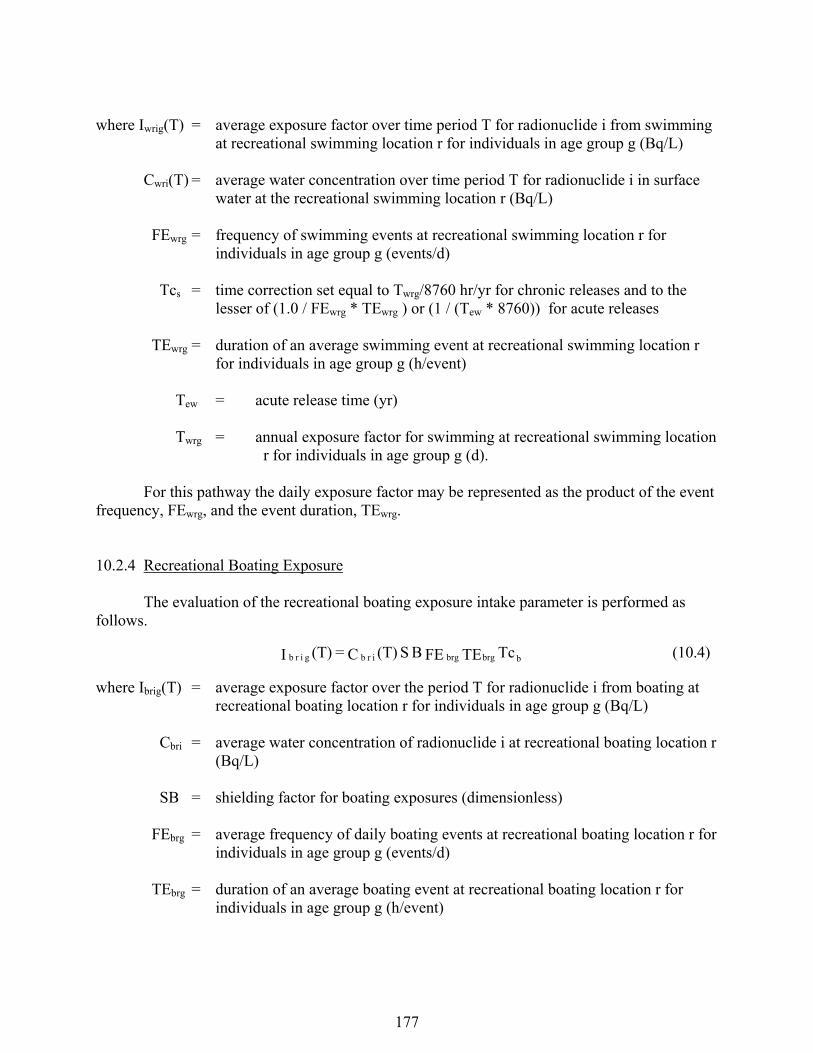
177

where Iwrig(T) = average exposure factor over time period T for radionuclide i from swimming at recreational swimming location r for individuals in age group g (Bq/L)

Cwri(T) = average water concentration over time period T for radionuclide i in surface

water at the recreational swimming location r (Bq/L) FEwrg = frequency of swimming events at recreational swimming location r for

individuals in age group g (events/d) Tcs = time correction set equal to Twrg/8760 hr/yr for chronic releases and to the

lesser of (1.0 / FEwrg * TEwrg ) or (1 / (Tew * 8760)) for acute releases TEwrg = duration of an average swimming event at recreational swimming location r

for individuals in age group g (h/event)

Tew = acute release time (yr) Twrg = annual exposure factor for swimming at recreational swimming location

r for individuals in age group g (d). For this pathway the daily exposure factor may be represented as the product of the event frequency, FEwrg, and the event duration, TEwrg. 10.2.4 Recreational Boating Exposure The evaluation of the recreational boating exposure intake parameter is performed as follows.

where Ibrig(T) = average exposure factor over the period T for radionuclide i from boating at recreational boating location r for individuals in age group g (Bq/L)

Cbri = average water concentration of radionuclide i at recreational boating location r

(Bq/L) SB = shielding factor for boating exposures (dimensionless) FEbrg = average frequency of daily boating events at recreational boating location r for

individuals in age group g (events/d) TEbrg = duration of an average boating event at recreational boating location r for

individuals in age group g (h/event)

bbrgbrg ir b g ir b Tc TE FE B S (T)C = (T)I (10.4)

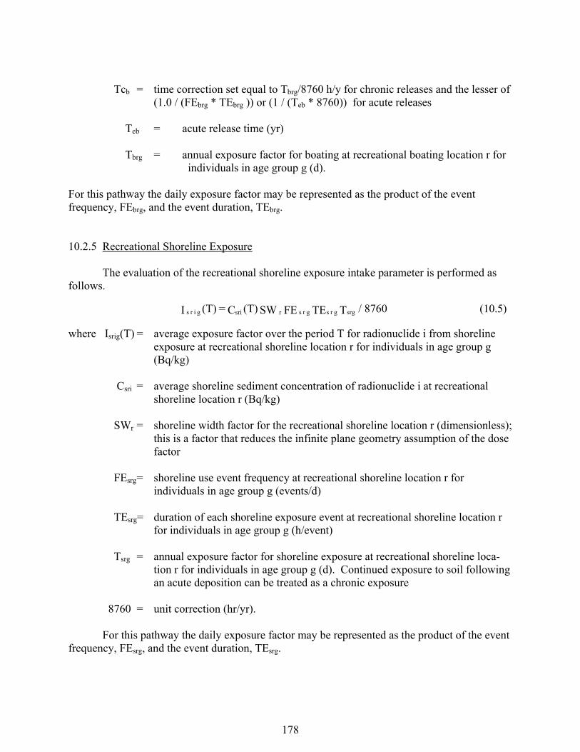
178

Tcb = time correction set equal to Tbrg/8760 h/y for chronic releases and the lesser of (1.0 / (FEbrg * TEbrg )) or (1 / (Teb * 8760)) for acute releases

Teb = acute release time (yr) Tbrg = annual exposure factor for boating at recreational boating location r for

individuals in age group g (d). For this pathway the daily exposure factor may be represented as the product of the event frequency, FEbrg, and the event duration, TEbrg. 10.2.5 Recreational Shoreline Exposure The evaluation of the recreational shoreline exposure intake parameter is performed as follows.

where Isrig(T) = average exposure factor over the period T for radionuclide i from shoreline exposure at recreational shoreline location r for individuals in age group g (Bq/kg)

Csri = average shoreline sediment concentration of radionuclide i at recreational

shoreline location r (Bq/kg) SWr = shoreline width factor for the recreational shoreline location r (dimensionless);

this is a factor that reduces the infinite plane geometry assumption of the dose factor

FEsrg = shoreline use event frequency at recreational shoreline location r for

individuals in age group g (events/d) TEsrg= duration of each shoreline exposure event at recreational shoreline location r

for individuals in age group g (h/event) Tsrg = annual exposure factor for shoreline exposure at recreational shoreline loca-

tion r for individuals in age group g (d). Continued exposure to soil following an acute deposition can be treated as a chronic exposure

8760 = unit correction (hr/yr). For this pathway the daily exposure factor may be represented as the product of the event frequency, FEsrg, and the event duration, TEsrg.

8760/T TE FE SW (T)C = (T)I srggr sgr s r srig ir s (10.5)

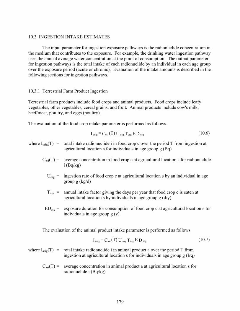
179

10.3 INGESTION INTAKE ESTIMATES The input parameter for ingestion exposure pathways is the radionuclide concentration in the medium that contributes to the exposure. For example, the drinking water ingestion pathway uses the annual average water concentration at the point of consumption. The output parameter for ingestion pathways is the total intake of each radionuclide by an individual in each age group over the exposure period (acute or chronic). Evaluation of the intake amounts is described in the following sections for ingestion pathways. 10.3.1 Terrestrial Farm Product Ingestion Terrestrial farm products include food crops and animal products. Food crops include leafy vegetables, other vegetables, cereal grains, and fruit. Animal products include cow's milk, beef/meat, poultry, and eggs (poultry). The evaluation of the food crop intake parameter is performed as follows.

where Icsig(T) = total intake radionuclide i in food crop c over the period T from ingestion at agricultural location s for individuals in age group g (Bq)

Ccsi(T) = average concentration in food crop c at agricultural location s for radionuclide

i (Bq/kg) Ucsg = ingestion rate of food crop c at agricultural location s by an individual in age

group g (kg/d) Tcsg = annual intake factor giving the days per year that food crop c is eaten at

agricultural location s by individuals in age group g (d/y) EDcsg = exposure duration for consumption of food crop c at agricultural location s for

individuals in age group g (y). The evaluation of the animal product intake parameter is performed as follows.

where Iasig(T) = total intake radionuclide i in animal product a over the period T from ingestion at agricultural location s for individuals in age group g (Bq)

Casi(T) = average concentration in animal product a at agricultural location s for

radionuclide i (Bq/kg)

DE T U (T)C = I csg csgcsg csicsig (10.6)

D E T U (T)C = I asg asgasg asiasig (10.7)

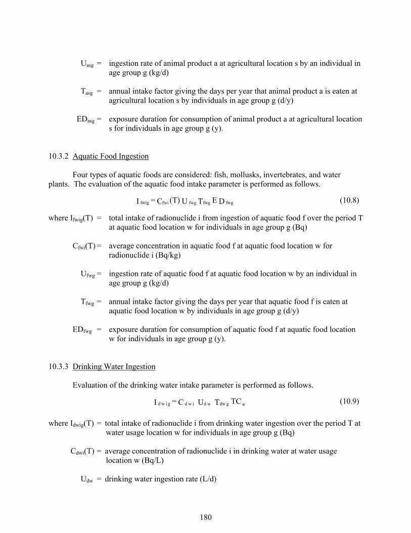
180

Uasg = ingestion rate of animal product a at agricultural location s by an individual in age group g (kg/d)

Tasg = annual intake factor giving the days per year that animal product a is eaten at

agricultural location s by individuals in age group g (d/y) EDasg = exposure duration for consumption of animal product a at agricultural location

s for individuals in age group g (y). 10.3.2 Aquatic Food Ingestion Four types of aquatic foods are considered: fish, mollusks, invertebrates, and water plants. The evaluation of the aquatic food intake parameter is performed as follows.

where Ifwig(T) = total intake of radionuclide i from ingestion of aquatic food f over the period T at aquatic food location w for individuals in age group g (Bq)

Cfwi(T) = average concentration in aquatic food f at aquatic food location w for

radionuclide i (Bq/kg) Ufwg = ingestion rate of aquatic food f at aquatic food location w by an individual in

age group g (kg/d) Tfwg = annual intake factor giving the days per year that aquatic food f is eaten at

aquatic food location w by individuals in age group g (d/y) EDfwg = exposure duration for consumption of aquatic food f at aquatic food location

w for individuals in age group g (y). 10.3.3 Drinking Water Ingestion Evaluation of the drinking water intake parameter is performed as follows.

where Idwig(T) = total intake of radionuclide i from drinking water ingestion over the period T at water usage location w for individuals in age group g (Bq)

Cdwi(T) = average concentration of radionuclide i in drinking water at water usage

location w (Bq/L) Udw = drinking water ingestion rate (L/d)

D E T U (T)C = I fwg fwgfwg fwifwig (10.8)

wgdw wdi wd gi wd TCT U C = I (10.9)

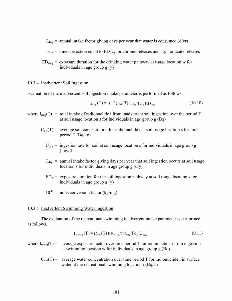
181

Tdwg = annual intake factor giving days per year that water is consumed (d/yr) TCw = time correction equal to EDdwg for chronic releases and Tdw for acute releases EDdwg = exposure duration for the drinking water pathway at usage location w for

individuals in age group g (y) 10.3.4 Inadvertent Soil Ingestion Evaluation of the inadvertent soil ingestion intake parameter is performed as follows.

where Idsig(T) = total intake of radionuclide i from inadvertent soil ingestion over the period T at soil usage location s for individuals in age group g (Bq)

Cdsi(T) = average soil concentration for radionuclide i at soil usage location s for time

period T (Bq/kg) Udsg = ingestion rate for soil at soil usage location s for individuals in age group g

(mg/d) Tdsg = annual intake factor giving days per year that soil ingestion occurs at soil usage

location s for individuals in age group g (d/y) EDds = exposure duration for the soil ingestion pathway at soil usage location s for

individuals in age group g (y) 10-6 = units conversion factor (kg/mg) 10.3.5 Inadvertent Swimming Water Ingestion The evaluation of the recreational swimming inadvertent intake parameter is performed as follows.

where Iwwig(T) = average exposure factor over time period T for radionuclide i from ingestion at swimming location w for individuals in age group g (Bq)

Cwri(T) = average water concentration over time period T for radionuclide i in surface

water at the recreational swimming location r (Bq/L)

ED T U (T)C 10 = (T)I dsgdsgdsgdsi6 -

g i s d (10.10)

swgswrggr wwrig i ww UTc TE FE (T)C = (T)I (10.11)

182

FEwrg = frequency of swimming events at water use location r for individuals in age group g (events/d)

TEwrg = duration of an average swimming event at water use location r for individuals

in age group g (h/event) Tcs = time correction set equal to Twrg for chronic releases and to the lesser of (Tew

* 8760 hr/yr / (FEwrg * TEwrg )) or (1 d) for acute releases

Twrg = annual exposure factor for swimming at water use location r for individuals in age group g (d)

Uswg = uptake rate of water while swimming for age group g (L/hr). For this pathway the daily exposure factor may be represented as the product of the event frequency, FEwrg, and the event duration, TEwrg. 10.3.6 Inadvertent Showering Water Ingestion The evaluation of the showering inadvertent intake parameter is performed as follows.

where Ihwig(T) = average exposure factor over time period T for radionuclide i from showering ingestion at location r for individuals in age group g (Bq)

Cdwi(T) = average concentration of radionuclide i in drinking water at water usage

location w (Bq/L) FEhrg = frequency of showering events at water use location r for individuals in age

group g (events/d) TEhrg = duration of an average shower event at water use location r for individuals in

age group g (h/event) Tcs = time correction set equal to Twrg for chronic releases and to the lesser of (Tew *

8760 hr/yr / (FEwrg * TEwrg )) or (1 d) for acute releases

Thrg = annual exposure factor for showering at water use location r for individuals in age group g (d)

Uhwg = uptake rate of water while showering for age group g (L/hr). For this pathway the daily exposure factor may be represented as the product of the event frequency, FEhrg, and the event duration, TEhrg.

hwgsrghgr h idwg i w h UTc TE FE (T)C = (T)I (10.12)

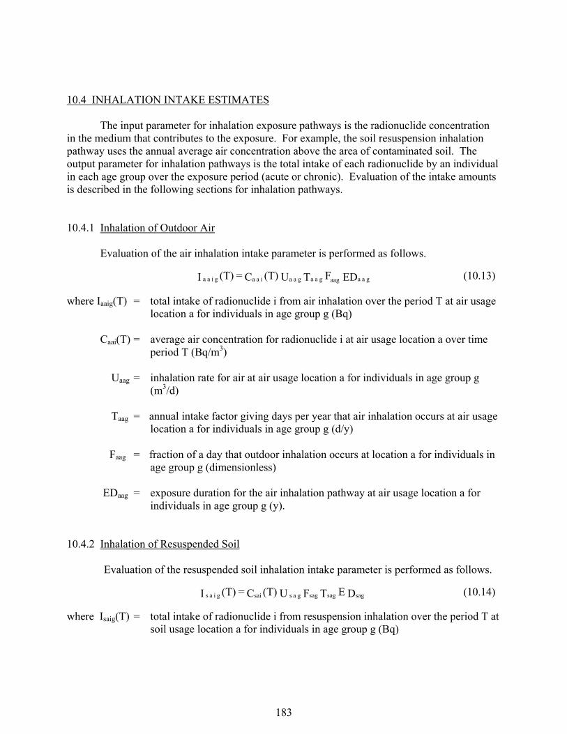
183

10.4 INHALATION INTAKE ESTIMATES The input parameter for inhalation exposure pathways is the radionuclide concentration in the medium that contributes to the exposure. For example, the soil resuspension inhalation pathway uses the annual average air concentration above the area of contaminated soil. The output parameter for inhalation pathways is the total intake of each radionuclide by an individual in each age group over the exposure period (acute or chronic). Evaluation of the intake amounts is described in the following sections for inhalation pathways. 10.4.1 Inhalation of Outdoor Air Evaluation of the air inhalation intake parameter is performed as follows.

where Iaaig(T) = total intake of radionuclide i from air inhalation over the period T at air usage location a for individuals in age group g (Bq)

Caai(T) = average air concentration for radionuclide i at air usage location a over time

period T (Bq/m3) Uaag = inhalation rate for air at air usage location a for individuals in age group g

(m3/d) Taag = annual intake factor giving days per year that air inhalation occurs at air usage

location a for individuals in age group g (d/y) Faag = fraction of a day that outdoor inhalation occurs at location a for individuals in

age group g (dimensionless) EDaag = exposure duration for the air inhalation pathway at air usage location a for

individuals in age group g (y). 10.4.2 Inhalation of Resuspended Soil Evaluation of the resuspended soil inhalation intake parameter is performed as follows.

where Isaig(T) = total intake of radionuclide i from resuspension inhalation over the period T at soil usage location a for individuals in age group g (Bq)

EDF T U (T)C = (T)I g a aaagg a ag a ai a ag i a a (10.13)

D E T F U (T)C = (T)I sagsagsagg a s saig i a s (10.14)

184

Csai(T)= average concentration of radionuclide i in air from resuspension over time period T at soil usage location s (Bq/m3)

Usag = inhalation rate of air for the resuspension pathway at soil usage location s for

individuals in age group g (m3/d) Fsag = fraction of a day that resuspension inhalation exposure occurs at soil usage

location s for individuals in age group g (dimensionless) Tsag = annual intake factor giving days per year that resuspension inhalation occurs

at soil usage location s for individuals in age group g (d/y) EDsag = exposure duration for the resuspension inhalation at soil usage location s for

individuals in age group g (y) 10.4.3 Indoor Inhalation of Contaminants Including Radon Evaluation of the indoor air inhalation intake parameter for contaminants is performed as follows.

where Ivwig(T) = total intake of radionuclide i from indoor air inhalation over the period T at water usage location w for individuals in age group g (Bq)

Caai(T) = average outdoor air concentration for radionuclide i at air usage location a

over time period T (Bq/m3) Cvwi(T) = average indoor air concentration for volatile radionuclide i at water usage

location w over time period T (Bq/m3) Uvwg = inhalation rate for indoor air at water usage location w for individuals in age

group g (m3/d) Fvwg = fraction of a day that indoor inhalation occurs at water usage location w for

individuals in age group g (dimensionless) Tvwg = annual intake factor giving days per year that indoor air inhalation occurs at

water usage location w for individuals in age group g (d/y) EDvwg = exposure duration for the indoor air inhalation pathway at water usage location

w for individuals in age group g (y).

ED T F U (T)]C)t(C[ = (T)I vwgvwgvwgvwgaai vwivwig (10.15)

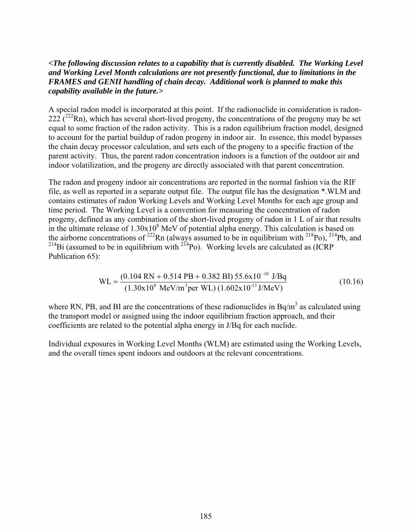
185

<The following discussion relates to a capability that is currently disabled. The Working Level and Working Level Month calculations are not presently functional, due to limitations in the FRAMES and GENII handling of chain decay. Additional work is planned to make this capability available in the future.> A special radon model is incorporated at this point. If the radionuclide in consideration is radon-222 (222Rn), which has several short-lived progeny, the concentrations of the progeny may be set equal to some fraction of the radon activity. This is a radon equilibrium fraction model, designed to account for the partial buildup of radon progeny in indoor air. In essence, this model bypasses the chain decay processor calculation, and sets each of the progeny to a specific fraction of the parent activity. Thus, the parent radon concentration indoors is a function of the outdoor air and indoor volatilization, and the progeny are directly associated with that parent concentration. The radon and progeny indoor air concentrations are reported in the normal fashion via the RIF file, as well as reported in a separate output file. The output file has the designation *.WLM and contains estimates of radon Working Levels and Working Level Months for each age group and time period. The Working Level is a convention for measuring the concentration of radon progeny, defined as any combination of the short-lived progeny of radon in 1 L of air that results in the ultimate release of 1.30x108 MeV of potential alpha energy. This calculation is based on the airborne concentrations of 222Rn (always assumed to be in equilibrium with 218Po), 214Pb, and 214Bi (assumed to be in equilibrium with 214Po). Working levels are calculated as (ICRP Publication 65):

J/MeV)(1.602x10WL)perMeV/m(1.30x10

J/Bq55.6x10BI)0.382PB0.514RN(0.104WL

13-38

10 (10.16)

where RN, PB, and BI are the concentrations of these radionuclides in Bq/m3 as calculated using the transport model or assigned using the indoor equilibrium fraction approach, and their coefficients are related to the potential alpha energy in J/Bq for each nuclide. Individual exposures in Working Level Months (WLM) are estimated using the Working Levels, and the overall times spent indoors and outdoors at the relevant concentrations.

186

11.0 DOSIMETRY AND HEALTH RISK MODULE Estimates of radiation dose and health risk are performed based on the intake and external exposure parameters generated by the intake component. Radiation dose is expressed as either committed equivalent dose to a specific organ, or as the committed effective dose to an individual. The health risk is expressed as the incremental risk of cancer incidence or mortality. The methods for estimation of radiation dose and health risk are discussed in the following sections. The input parameters for the dose and health risk evaluation are the intake parameters (for ingestion and inhalation) or the medium concentration average parameters and exposure times (for external exposure pathways) as generated by the intake component (defined in Section 10). Table 11.1 summarizes these parameters. 11.1 COMMUNICATION INTERFACES The input files for the individual intake module are the global input data file (GID) and the receptor intake output file (RIF). Several auxiliary data communication files are needed if Federal Guidance Report 13 doses or risks are requested (index file, two ingestion dose and risk factor files, two inhalation dose and risk factor files, and external dose factor files for air, soil, and water). Other dosimetry data are taken from the FRAMES database via the GID file. The receptor intake output file (RIF) is generated by the individual intake module (or other external program that is capable of generating the proper file information). The GID file section for the impacts module is generated by the user interface program. It contains information describing the scope of the analysis and all user-provided input parameters for an analysis. The structure and content of the files are given in Appendices A and B. The output from the impacts module is the annualized dose and risk from contaminants in various media to which individuals or populations are exposed. This information is provided in a primary data communication file, the health impacts output file (HIF). 11.2 RADIATION DOSE ASSESSMENT The endpoints for radiation dose depend on the dose factors used as the basis of the analysis. Three sources of dose factors are in general use: 1) EPA supported values published in Federal Guidance Reports 11 and 12, 2) DOE supported values published in DOE reports, and 3) age dependent dose factors in reports of the International Commission on Radiological Protection (ICRP). All of these sources are based on recommendations of the ICRP. Each set of dose factors is described in the following sections. Differences in parameter assumptions exist for some radionuclides between the EPA, DOE, and ICRP dosimetry, which have resulted in numerical differences between dose factors. The EPA and DOE sources are essentially equivalent (rounding error); the differences between these and the more-recent ICRP sources relate primarily to changes in the weighting factors used for effective dose equivalent versus effective dose coefficients (a change in definition).

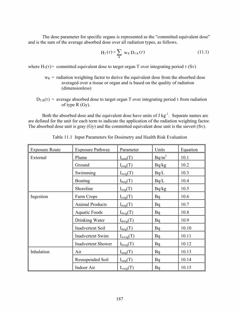
187

The dose parameter for specific organs is represented as the "committed equivalent dose" and is the sum of the average absorbed dose over all radiation types, as follows.

where HT() = committed equivalent dose to target organ T over integrating period (Sv) wR = radiation weighting factor to derive the equivalent dose from the absorbed dose

averaged over a tissue or organ and is based on the quality of radiation (dimensionless)

DT,R() = average absorbed dose to target organ T over integrating period from radiation

of type R (Gy). Both the absorbed dose and the equivalent dose have units of J kg-1. Separate names are are defined for the unit for each term to indicate the application of the radiation weighting factor. The absorbed dose unit is gray (Gy) and the committed equivalent dose unit is the sievert (Sv). Table 11.1 Input Parameters for Dosimetry and Health Risk Evaluation

Exposure Route Exposure Pathway Parameter Units Equation

External Plume Ieaig(T) Bq/m3 10.1

Ground Iesig(T) Bq/kg 10.2

Swimming Iwrig(T) Bq/L 10.3

Boating Ibrig(T) Bq/L 10.4

Shoreline Isrig(T) Bq/kg 10.5

Ingestion Farm Crops Icsig(T) Bq 10.6

Animal Products Iasig(T) Bq 10.7

Aquatic Foods Ifwig(T) Bq 10.8

Drinking Water Idwig(T) Bq 10.9

Inadvertent Soil Idsig(T) Bq 10.10

Inadvertent Swim Iwwig(T) Bq 10.11

Inadvertent Shower Ihwig(T) Bq 10.12

Inhalation Air Iaaig(T) Bq 10.13

Resuspended Soil Isaig(T) Bq 10.14

Indoor Air Ivwig(T) Bq 10.15

)(D w = )(H RT,RR

T (11.1)

188

The dose parameter representing the total effect to the body is the committed effective dose, E(). This parameter is estimated as the sum of the products of the committed organ or tissue equivalent doses and the appropriate organ or tissue weighting factors (wT), over the integrating time, . The committed effective dose is calculated from the committed equivalent dose as follows.

where E() = committed effective dose over integrating period (Sv) wT = tissue weighting factor, by which the equivalent dose in a tissue or organ is

weighted to represent the relative contribution of that tissue or organ to the total detriment resulting from uniform irradiation of the body (dimensionless)

and HT() is calculated as per Equation (11.1). The units of the committed effective dose are the same as the units of the committed equivalent dose (Sv). The time period of integration for worker dose coefficients is 50 years. The integration period for age-dependent dose coefficients is from the time of intake to 70 years. The age-dependent dose coefficients are provided for the age groups listed in Table 11.2. A change in dose terminology occurred with release of ICRP Publication 60. Prior to this publication the effective dose, E(), was called the committed effective dose equivalent (CEDE). Also, the equivalent dose was previously called the dose equivalent. In the following discussions, the current terms are used: the CEDE is referred to as effective dose and the dose equivalent is referred to as the equivalent dose. Table 11.2 Age-dependent Dose Coefficient Age Groups

Age at Intake Age Range Integrating Time,

3 mo 0 - 12 mo 69.75 y

1 y 1 - 2 y 69 y

5 y >2 - 7 y 65 y

10 y >7 - 12 y 60 y

15 y >12 - 17 y 55 y

Adult > 17 y 50 y

)(H w = )E( TTT

(11.2)

189

The dose coefficients are defined for several exposure routes and media and, in some cases, as a function of age. The nomenclature for representation of the dose coefficients is indicated in Table 11.3. 11.2.1 Federal Guidance Report Dose Coefficients The EPA dose coefficients are provided in Federal Guidance Reports (FGR) 11 and 12 (EPA 1988 and EPA 1993). Coefficient values of organ-specific dose equivalent and effective dose equivalent are provided for inhalation and ingestion in FGR 11, and for external exposure to air, water, and soil in FGR 12. The internal dose coefficient values are based primarily on recommendations in ICRP Publications 26 and 30, and are to be used for evaluation of dose to adults (workers). The integration period for internal dose conversion factors is 50 years. The external dose conversion factors are also based on ICRP Publication 30 tissue weighting factors. These are included in the GENII-V2 libraries under the general heading of “ICRP-30/48.” 11.2.2 Department of Energy Dose Coefficients The DOE (1988a and 1988b) values are for workers and are based on ICRP Publications 26 and 30. They provide estimates of dose equivalent for specific organs in addition to the effective dose equivalent. There are some differences in the numerical evaluation of dose coefficients between the DOE publication and the EPA FGR publications and differences in numerical values can be found. Dose coefficients are provide for inhalation and ingestion intakes in DOE (1988b) and for external exposure to air, ground, and water in DOE (1988a). These are similar enough to the EPA guidance that the ICRP-30/48 values are used for both. 11.2.3 Current ICRP Dose Coefficients The ICRP has published dose coefficients for estimation of dose to workers and to members of the public. Worker committed effective dose factors are based on a 50 year work period with the target individual being an adult. Worker dose coefficients are given in ICRP Publications 68. The ICRP age-dependent committed equivalent dose coefficients are for estimation of dose to the public. Age-dependent committed equivalent dose and committed effective dose coefficient values for ingestion are given in ICRP Publications 56, 67, and 69, and values for inhalation are given in ICRP Publication 71. ICRP Publication 72 presents committed effective dose coefficients as a function of age for ingestion and inhalation (organ specific committed equivalent dose coefficients are not presented in this publication). Table 11.4 summarizes the content of each of these reports. These values form the underlying basis for Federal Guidance Report 13; they are included in the GENII-V2 libraries under the general heading of “ICRP-60.”

190

Table 11.3 Dose and Risk Coefficient Nomenclature

Subscript Description

Dose Coefficient General Symbol

Position

Uses

Effective Dose (and Effective Dose Equivalent)

EC123 1 2 3

radionuclide - i age group g - general a - adult exposure route/medium a - external, air g - external, ground o - ingestion, oral r - inhalation, respiration w - external, water

Equivalent Dose (and Dose Equivalent)

HC1234 1,2,3 4 5

same as above inhalation or ingestion class – c inhalation (F,M,S) ingestion (f1) organ - T

11.2.4 External Exposure Pathway Dose Assessment Radiation dose from external exposure pathways is evaluated using the average medium concentrations, the exposure times, and the external dose coefficient appropriate to the medium. The external dose coefficients are provided for exposure of adults in FGR 12 (EPA 1993) in terms of equivalent dose to specific organs and the effective dose for an individual. The dose coefficients are presented as dose rate factors that are multiplied by the medium average concentration and exposure time to give the total radiation dose for the defined exposure period. The following equations describe estimation of the equivalent dose and effective dose from external exposure pathways. External Exposure from Air Immersion The evaluation of radiation dose from a plume of radioactivity may be evaluated using the finite plume model or the semi-infinite plume model. When the finite plume model is used the dose is evaluated by the atmospheric transport component (Section 5.4) because the dose is a function of plume dimensions. When the semi-infinite plume model is used, the atmospheric transport analysis provides the time-integral of

191

Table 11.4 Summary of ICRP Publication Dose Coefficients

Publication No. Target Group

Dose Type

Intake Route

Lung Model

Elements Basis for wT

56 (1989) Public, Part 1

E() HT()

Ingestion NA H, C, Sr, Zr, Nb, Ru, I, Cs, Ce, Pu, Am, Np

ICRP 26

67 (1993) Public, Part 2

E() HT()

Ingestion NA S, Co, Ni, Zn, Sr, Mo, Tc, Ag, Te, Ba, Pb, Po, Ra

ICRP 60

68 (1994) Workers

E(50) Inhalation Ingestion

ICRP 66 Most ICRP 60

69 (1995) Public, Part 3

E() HT()

Ingestion NA Fe, Se, Sb, Th, U ICRP 60

71 (1995) Public, Part 4

E() HT()

Inhalation ICRP 66 H, C, S, Ca, Fe, Co, Ni, Zn, Se, Sr, Zr, Nb, Mo, Tc, Ru, Ag, Sb, Te, I, Cs, Ba, Ce, Pb, Po, Ra, Th, Np, Pu, Am, Cm

ICRP 60

72 (1996a) Public, Part 5

E() Inhalation Ingestion

ICRP 66 Most ICRP 60

plume concentration at the exposure locations, which is used in the analysis described here. For the semi-infinite plume model, the equivalent dose from external exposure is evaluated as follows.

where IHeaigT(T) = equivalent dose to organ or tissue T from external exposure to radionuclide i from plume immersion at air usage location a for an individual in age group g (Sv)

Ieaig(T) = external exposure average air concentration for radionuclide i for plume

immersion at air usage location a for individuals in age group g (Bq/m3) HCiaaT = equivalent dose coefficient for air immersion to an organ T, radionuclide i,

for an adult (Sv m3 per Bq s) TEa = time of exposure, either Tex for acute releases or Tyr for chronic releases (y) 3.15x107 = units correction (s/y). The effective dose from external exposure from immersion in an airborne plume is evaluated as follows.

7aiaaT eaigeaigT 10x15.3TEHC (T)I = (T)IH (11.3)

192

where IEeaig(T) = effective dose from external exposure to radionuclide i from plume immersion at air usage location a for an individual in age group g (Sv)

Ieaig(T) = external exposure average air concentration for radionuclide i for plume

immersion at air usage location a for individuals in age group g (Bq/m3) ECiaa = effective dose coefficient for external exposure from plume immersion for

radionuclide i for an adult (Sv m3 per Bq s). TEa = time of exposure, either Tex for acute releases or Tyr for chronic releases (y) 3.15x107 = units correction (s/y). As indicated in these equations, the adult equivalent dose (HCiaaT) and effective dose coefficients (ECiaa) are used for all age groups, as represented by the subscript "a" (adult) in place of the general age group subscript "g". This is a necessary approximation because age-dependent effective dose coefficients are not available for external exposures, although ICRP indicates that external doses to adults and children do not differ greatly at most photon energies of concern (ICRP 1996b). External Exposure from Ground Contamination The equivalent dose from external exposure to contaminated ground is evaluated as follows.

where IHesigT(T) = equivalent dose to organ T from external exposure to radionuclide i from contaminated soil at soil usage location s for an individual in age group g for exposure over time period T (Sv)

Iesig(T) = external exposure average soil concentration for radionuclide i at soil usage

location s for individuals in age group g for exposure over time period T (Bq/kg)

HCiagT = equivalent dose coefficient to organ T for external exposure to ground for

radionuclide i for an adult (Sv m2 per Bq s) TEg = time of exposure, either Teg for acute releases or Tyr for chronic releases (y) s = surface soil bulk density (kg/m3) ds = thickness of surface soil layer (m) 3.15x107 = units correction (s/y).

7aiaa eaigeaig 10x15.3TEEC (T)I = (T)IE (11.4)

ss7

giagTesigesigT dρ3.15x10TEHC (T)I = (T)IH (11.5)

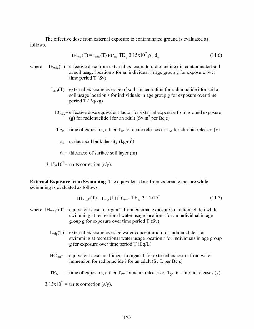
193

The effective dose from external exposure to contaminated ground is evaluated as follows.

where IEesig(T) = effective dose from external exposure to radionuclide i in contaminated soil at soil usage location s for an individual in age group g for exposure over time period T (Sv)

Iesig(T) = external exposure average of soil concentration for radionuclide i for soil at

soil usage location s for individuals in age group g for exposure over time period T (Bq/kg)

ECiag = effective dose equivalent factor for external exposure from ground exposure

(g) for radionuclide i for an adult (Sv m2 per Bq s) TEg = time of exposure, either Teg for acute releases or Tyr for chronic releases (y) s = surface soil bulk density (kg/m3) ds = thickness of surface soil layer (m) 3.15x107 = units correction (s/y). External Exposure from Swimming The equivalent dose from external exposure while swimming is evaluated as follows.

where IHwrigT(T) = equivalent dose to organ T from external exposure to radionuclide i while swimming at recreational water usage location r for an individual in age group g for exposure over time period T (Sv)

Iwrig(T) = external exposure average water concentration for radionuclide i for

swimming at recreational water usage location r for individuals in age group g for exposure over time period T (Bq/L)

HCiagT = equivalent dose coefficient to organ T for external exposure from water

immersion for radionuclide i for an adult (Sv L per Bq s) TEw = time of exposure, either Tew for acute releases or Tyr for chronic releases (y) 3.15x107 = units correction (s/y).

ss7

giagesigesig d10x15.3TEEC (T)I = (T)IE (11.6)

7wiawTwrigwrigT 1015.3TEHC (T)I= (T)IH x (11.7)

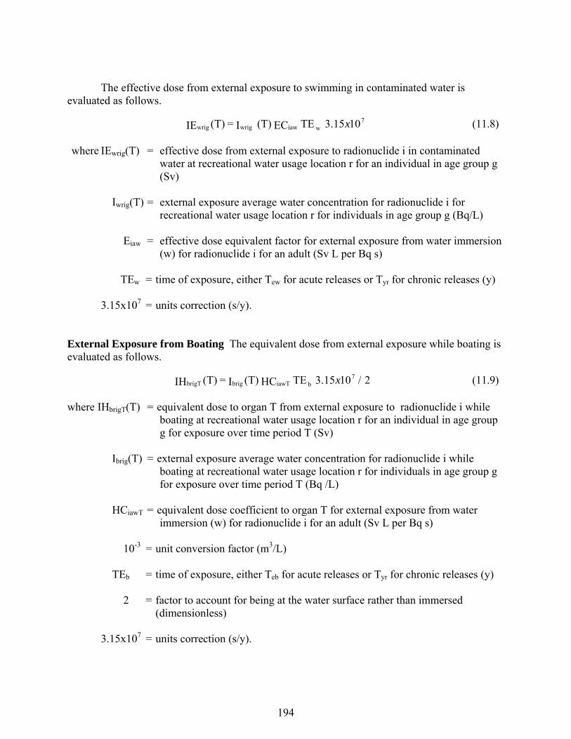
194

The effective dose from external exposure to swimming in contaminated water is evaluated as follows.

where IEwrig(T) = effective dose from external exposure to radionuclide i in contaminated water at recreational water usage location r for an individual in age group g (Sv)

Iwrig(T) = external exposure average water concentration for radionuclide i for

recreational water usage location r for individuals in age group g (Bq/L) Eiaw = effective dose equivalent factor for external exposure from water immersion

(w) for radionuclide i for an adult (Sv L per Bq s) TEw = time of exposure, either Tew for acute releases or Tyr for chronic releases (y) 3.15x107 = units correction (s/y). External Exposure from Boating The equivalent dose from external exposure while boating is evaluated as follows.

where IHbrigT(T) = equivalent dose to organ T from external exposure to radionuclide i while boating at recreational water usage location r for an individual in age group g for exposure over time period T (Sv)

Ibrig(T) = external exposure average water concentration for radionuclide i while

boating at recreational water usage location r for individuals in age group g for exposure over time period T (Bq /L)

HCiawT = equivalent dose coefficient to organ T for external exposure from water

immersion (w) for radionuclide i for an adult (Sv L per Bq s) 10-3 = unit conversion factor (m3/L) TEb = time of exposure, either Teb for acute releases or Tyr for chronic releases (y) 2 = factor to account for being at the water surface rather than immersed

(dimensionless) 3.15x107 = units correction (s/y).

7wiawwrigwrig 1015.3TEEC (T) I = (T)IE x (11.8)

2/1015.3TEHC (T)I = (T)IH7

biawTbrigbrigT x (11.9)

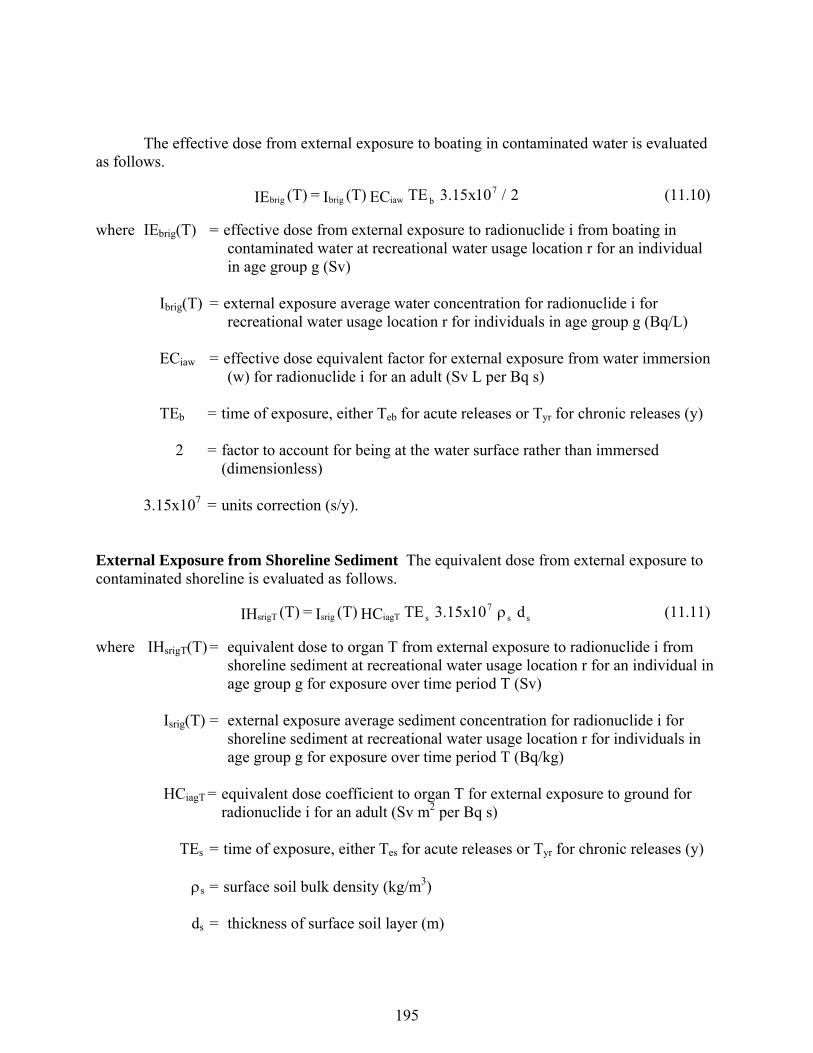
195

The effective dose from external exposure to boating in contaminated water is evaluated as follows.

where IEbrig(T) = effective dose from external exposure to radionuclide i from boating in contaminated water at recreational water usage location r for an individual in age group g (Sv)

Ibrig(T) = external exposure average water concentration for radionuclide i for

recreational water usage location r for individuals in age group g (Bq/L) ECiaw = effective dose equivalent factor for external exposure from water immersion

(w) for radionuclide i for an adult (Sv L per Bq s) TEb = time of exposure, either Teb for acute releases or Tyr for chronic releases (y) 2 = factor to account for being at the water surface rather than immersed

(dimensionless) 3.15x107 = units correction (s/y). External Exposure from Shoreline Sediment The equivalent dose from external exposure to contaminated shoreline is evaluated as follows.

where IHsrigT(T) = equivalent dose to organ T from external exposure to radionuclide i from shoreline sediment at recreational water usage location r for an individual in age group g for exposure over time period T (Sv)

Isrig(T) = external exposure average sediment concentration for radionuclide i for

shoreline sediment at recreational water usage location r for individuals in age group g for exposure over time period T (Bq/kg)

HCiagT = equivalent dose coefficient to organ T for external exposure to ground for

radionuclide i for an adult (Sv m2 per Bq s) TEs = time of exposure, either Tes for acute releases or Tyr for chronic releases (y) s = surface soil bulk density (kg/m3) ds = thickness of surface soil layer (m)

2/10x15.3TEEC (T)I = (T)IE7

biawbrigbrig (11.10)

ss7

siagTsrigsrigT d10x15.3TEHC (T)I = (T)IH (11.11)

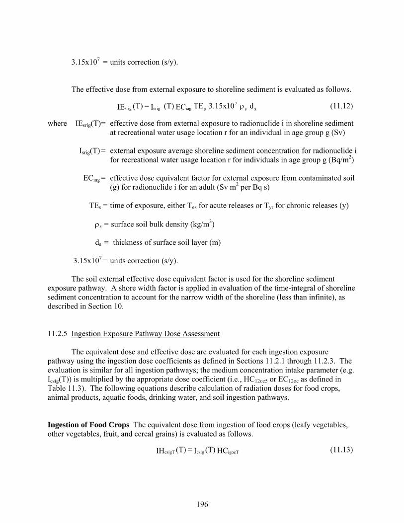
196

3.15x107 = units correction (s/y). The effective dose from external exposure to shoreline sediment is evaluated as follows.

where IEsrig(T) = effective dose from external exposure to radionuclide i in shoreline sediment at recreational water usage location r for an individual in age group g (Sv)

Isrig(T) = external exposure average shoreline sediment concentration for radionuclide i

for recreational water usage location r for individuals in age group g (Bq/m2) ECiag = effective dose equivalent factor for external exposure from contaminated soil

(g) for radionuclide i for an adult (Sv m2 per Bq s) TEs = time of exposure, either Tes for acute releases or Tyr for chronic releases (y) s = surface soil bulk density (kg/m3) ds = thickness of surface soil layer (m) 3.15x107 = units correction (s/y). The soil external effective dose equivalent factor is used for the shoreline sediment exposure pathway. A shore width factor is applied in evaluation of the time-integral of shoreline sediment concentration to account for the narrow width of the shoreline (less than infinite), as described in Section 10. 11.2.5 Ingestion Exposure Pathway Dose Assessment The equivalent dose and effective dose are evaluated for each ingestion exposure pathway using the ingestion dose coefficients as defined in Sections 11.2.1 through 11.2.3. The evaluation is similar for all ingestion pathways; the medium concentration intake parameter (e.g. Icsig(T)) is multiplied by the appropriate dose coefficient (i.e., HC12oc5 or EC12oc as defined in Table 11.3). The following equations describe calculation of radiation doses for food crops, animal products, aquatic foods, drinking water, and soil ingestion pathways. Ingestion of Food Crops The equivalent dose from ingestion of food crops (leafy vegetables, other vegetables, fruit, and cereal grains) is evaluated as follows.

ss7

siagsrigsrig d10x15.3TEEC (T) I = (T)IE (11.12)

HC (T)I = (T)IH igocTcsigcsigT (11.13)

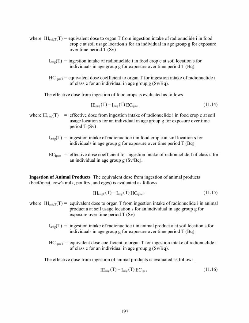
197

where IHcsigT(T) = equivalent dose to organ T from ingestion intake of radionuclide i in food crop c at soil usage location s for an individual in age group g for exposure over time period T (Sv)

Icsig(T) = ingestion intake of radionuclide i in food crop c at soil location s for

individuals in age group g for exposure over time period T (Bq) HCigocT = equivalent dose coefficient to organ T for ingestion intake of radionuclide i

of class c for an individual in age group g (Sv/Bq). The effective dose from ingestion of food crops is evaluated as follows.

where IEcsig(T) = effective dose from ingestion intake of radionuclide i in food crop c at soil usage location s for an individual in age group g for exposure over time period T (Sv)

Icsig(T) = ingestion intake of radionuclide i in food crop c at soil location s for

individuals in age group g for exposure over time period T (Bq) ECigoc = effective dose coefficient for ingestion intake of radionuclide I of class c for

an individual in age group g (Sv/Bq). Ingestion of Animal Products The equivalent dose from ingestion of animal products (beef/meat, cow's milk, poultry, and eggs) is evaluated as follows.

where IHasigT(T) = equivalent dose to organ T from ingestion intake of radionuclide i in animal product a at soil usage location s for an individual in age group g for exposure over time period T (Sv)

Iasig(T) = ingestion intake of radionuclide i in animal product a at soil location s for

individuals in age group g for exposure over time period T (Bq) HCigocT = equivalent dose coefficient to organ T for ingestion intake of radionuclide i

of class c for an individual in age group g (Sv/Bq). The effective dose from ingestion of animal products is evaluated as follows.

EC (T)I = (T)IE cigocsigcsig (11.14)

HC (T)I = (T)IH TcigoasigasigT (11.15)

EC (T)I = (T)IE cigoasigasig (11.16)

198

where IEasig(T) = effective dose from ingestion intake of radionuclide i in animal product a at soil usage location s for an individual in age group g for exposure over time period T (Sv)

Iasig(T) = ingestion intake of radionuclide i in animal product a at soil location s for

individuals in age group g for exposure over time period T (Bq) ECigoc = effective dose coefficient for ingestion intake of radionuclide i for an

individual in age group g (Sv/Bq). Ingestion of Aquatic Foods The equivalent dose from ingestion of aquatic foods (fish, crustaceans, mollusks, and aquatic plants) is evaluated as follows.

where IHfwigT(T) = equivalent dose to organ T from ingestion intake of radionuclide i in aquatic food f at water usage location w for an individual in age group g for exposure over time period T (Sv)

Ifwig(T) = ingestion intake of radionuclide i in aquatic food f at water usage location w

for individuals in age group g for exposure over time period T (Bq) HCigocT = equivalent dose coefficient to organ T for ingestion intake of radionuclide i

of class c for an individual in age group g (Sv/Bq). The effective dose from ingestion of aquatic foods is evaluated as follows.

where IEfwig(T) = effective dose from ingestion intake of radionuclide i in aquatic food f at water usage location w for an individual in age group g for exposure over time period T (Sv)

Ifwig(T) = ingestion intake of radionuclide i in aquatic food f at water usage location w

for individuals in age group g for exposure over time period T (Bq) ECigoc = effective dose coefficient for ingestion intake of radionuclide i of class c for

an individual in age group g (Sv/Bq). Ingestion of Drinking Water The equivalent dose from ingestion of drinking water is evaluated as follows.

HC (T)I = (T)IH TcigofwigfwigT (11.17)

EC (T)I = (T)IE cigofwigfwig (11.18)

HC (T)I = (T)IH TcigodwigdwigT (11.19)

199

where IHdwigT(T) = equivalent dose to organ T from ingestion intake of radionuclide i in drinking

water at water usage location w for an individual in age group g for exposure over time period T (Sv)

Idwig(T) = ingestion intake of radionuclide i in drinking water at water usage location w

for individuals in age group g for exposure over time period T (Bq) HCigocT = equivalent dose coefficient to organ T for ingestion intake of radionuclide i

of class c for an individual in age group g (Sv/Bq). The effective dose from ingestion of drinking water is evaluated as follows.

where IEdwig(T) = effective dose from ingestion intake of radionuclide i in drinking water at water usage location w for an individual in age group g for exposure over time period T (Sv)

Idwig(T) = ingestion intake of radionuclide i in drinking water at water usage location w

for individuals in age group g for exposure over time period T (Bq) ECigoc = effective dose coefficient for ingestion intake of radionuclide i of class c for

an individual in age group g (Sv/Bq). Ingestion of Soil The equivalent dose from inadvertent ingestion of soil is evaluated as follows.

where IHdsigT(T) = equivalent dose to organ T from ingestion intake of radionuclide i in soil at soil usage location s for an individual in age group g for exposure over time period T (Sv)

Idsig(T) = ingestion intake of radionuclide i in soil at soil location s for individuals in

age group g for exposure over time period T (Bq) HCigocT = equivalent dose coefficient to organ T for ingestion intake of radionuclide i

of class c for an individual in age group g (Sv/Bq). The effective dose from inadvertent ingestion of soil is evaluated as follows.

EC (T)I = (T)IE cigodwigdwig (11.20)

HC (T)I = (T)IH TcigodsigdsigT (11.21)

EC (T)I = (T)IE cigodsigdsig (11.22)

200

where IEdsig(T) = effective dose from ingestion intake of radionuclide i in soil at soil usage location s for an individual in age group g for exposure over time period T (Sv)

Idsig(T) = ingestion intake of radionuclide i in soil at soil location s for individuals in

age group g for exposure over time period T (Bq) ECigoc = effective dose coefficient for ingestion intake of radionuclide i of class c for

an individual in age group g (Sv/Bq). Ingestion of Water While Swimming The equivalent dose from inadvertent ingestion of water while swimming is evaluated as follows.

where IHwwigT(T) = equivalent dose to organ T from ingestion intake of radionuclide i in water at water usage location w for an individual in age group g for exposure over time period T (Sv)

Iwwig(T) = ingestion intake of radionuclide i while swimming at water usage location w

for individuals in age group g for exposure over time period T (Bq) HCigocT = equivalent dose coefficient to organ T for ingestion intake of radionuclide i

of class c for an individual in age group g (Sv/Bq). The effective dose from inadvertent ingestion of water while swimming is evaluated as follows.

where IEwwig(T) = effective dose from ingestion intake of radionuclide i in swimming water at water usage location w for an individual in age group g for exposure over time period T (Sv)

Iwwig(T) = ingestion intake of radionuclide i in swimming water at water usage location

w for individuals in age group g for exposure over time period T (Bq) ECigoc = effective dose coefficient for ingestion intake of radionuclide i of class c for

an individual in age group g (Sv/Bq). Ingestion of Water While Showering The equivalent dose from inadvertent ingestion of water while showering is evaluated as follows.

HC (T)I = (T)IH TcigowigwwigTw (11.23)

EC (T)I = (T)IE cigowigwwigw (11.24)

HC (T)I = (T)IH TcigowighwigTh (11.25)

201

where IHhwigT(T) = equivalent dose to organ T from ingestion intake of radionuclide i in shower water at water usage location w for an individual in age group g for exposure over time period T (Sv)

Ihwig(T) = ingestion intake of radionuclide i in shower water at water usage location w

for individuals in age group g for exposure over time period T (Bq) HCigocT = equivalent dose coefficient to organ T for ingestion intake of radionuclide i

of class c for an individual in age group g (Sv/Bq). The effective dose from inadvertent ingestion of shower water is evaluated as follows.

where IEhwig(T) = effective dose from ingestion intake of radionuclide i in shower water at water usage location w for an individual in age group g for exposure over time period T (Sv)

Ihwig(T) = ingestion intake of radionuclide i in shower water at water usage location w

for individuals in age group g for exposure over time period T (Bq) ECigoc = effective dose coefficient for ingestion intake of radionuclide i of class c for

an individual in age group g (Sv/Bq). 11.2.6 Inhalation Exposure Pathway Dose Assessment The equivalent dose and effective dose are evaluated for each inhalation exposure pathway using the inhalation dose coefficients as defined in Sections 11.1.1 through 11.1.3. The evaluation is similar for all inhalation pathways; the medium concentration intake parameter (e.g. Icsig(T)) is multiplied by the appropriate dose coefficient (i.e., HC12rc5 or EC12rc as defined in Table 11.3). The following equations describe calculation of radiation doses for inhalation of air, resuspended soil, and indoor air contaminants. NOTE: inhalation of tritium gas (HT) is a special case – the code assumes fractional conversion to HTO, which is inhaled (see Section 9.6.1). Inhalation of Air The equivalent dose from inhalation of air is evaluated as follows.

where IHaaigT(T) = equivalent dose to organ T from inhalation intake of radionuclide i in air at air usage location a for an individual in age group g for exposure over time period T (Sv)

Iaaig(T) = inhalation intake of radionuclide i in air at air usage location a for

individuals in age group g for exposure over time period T (Bq)

EC (T)I = (T)IE cigowighwigh (11.26)

HC (T)I = (T)IH TcigraaigaaigT (11.27)

202

HCigrcT = equivalent dose coefficient to organ T for inhalation intake of radionuclide i of class c for an individual in age group g (Sv/Bq).

The effective dose from inhalation of air is evaluated as follows.

where IEaaig(T) = effective dose from inhalation intake of radionuclide i in air at air usage location a for an individual in age group g for exposure over time period T (Sv)

Iaaig(T) = inhalation intake of radionuclide i in air at air usage location a for individuals

in age group g for exposure over time period T (Bq) ECigrc = effective dose coefficient for inhalation intake of radionuclide i oc class c for

an individual in age group g (Sv/Bq). Inhalation of Resuspended Soil The equivalent dose from inhalation of resuspended soil is evaluated as follows.

where IHsaigT(T) = equivalent dose to organ T from inhalation intake of radionuclide i in resuspended soil at air usage location a for an individual in age group g for exposure over time period T (Sv)

Isaig(T) = inhalation intake of radionuclide i in resuspended soil at air usage location a

for individuals in age group g for exposure over time period T (Bq) HCigrcT = equivalent dose coefficient to organ T for inhalation intake of radionuclide i

of class c for an individual in age group g (Sv/Bq). The effective dose from inhalation of resuspended soil is evaluated as follows.

where IEsaig(T) = effective dose from inhalation intake of radionuclide i in resuspended soil at air usage location a for an individual in age group g for exposure over time period T (Sv)

Isaig(T) = inhalation intake of radionuclide i in resuspended soil at air usage location a

for individuals in age group g for exposure over time period T (Bq) ECigrc = effective dose coefficient for inhalation intake of radionuclide i of class c for

an individual in age group g (Sv/Bq).

EC (T)I = (T)IE cigraaigaaig (11.28)

HC (T)I = (T)IH TcigrsaigsaigT (11.29)

EC (T)I = (T)IE cigrsaigsaig (11.30)

203

Inhalation of Indoor Air The equivalent dose from inhalation of contaminants in indoor air is evaluated as follows.

where IHvwigT(T) = equivalent dose to organ T from inhalation intake of radionuclide i in indoor

air at location w for an individual in age group g for exposure over time period T (Sv)

Ivwig(T) = inhalation intake of radionuclide i in indoor air at location w for individuals

in age group g for exposure over time period T (Bq) HCigrcT = equivalent dose coefficient to organ T for inhalation intake of radionuclide i

of class c for an individual in age group g (Sv/Bq). The effective dose from inhalation in indoor air is evaluated as follows.

where IEvwig(T) = effective dose from inhalation intake of radionuclide i in indoor air at location w for an individual in age group g for exposure over time period T (Sv)

Ivwig(T) = inhalation intake of radionuclide i in indoor air at location w for individuals

in age group g for exposure over time period T (Bq) ECigrc = effective dose coefficient for inhalation intake of radionuclide i of class c for

an individual in age group g (Sv/Bq). 11.3 HEALTH RISK ASSESSMENT Three primary methods are available to perform the assessment of health impacts: 1) use of effective dose estimates multiplied by health effects conversion factors, 2) use of intake estimates multiplied by cancer incidence slope factor published in EPA Health Effects Assessment Summary Tables, 3) calculation using organ-dependent health effect conversion factors. Each of these methods is discussed in the following sections. 11.3.1 Use of Effective Dose An estimate of the health impacts, expressed as risk of a defined health effect, can be

HC (T)I = (T)IH TcigrvwigvwigT (11.31)

EC (T)I = (T)IE cigrvwigvwig (11.32)

204

made from the effective dose and appropriate health effect conversion factors. The health effect conversion factors (“Risk coefficients”) must be defined for each age group or for adults and must be representative of the exposed population (i.e., workers or the public). General health effect conversion factors are presented in ICRP Publication 60 (1990) for exposure of workers and the adult population for health effects expressed as fatal cancer, non-fatal cancer, and severe hereditary effects. Estimation of the health impacts is performed as follows for exposure pathway 1, medium 2, radionuclide i, age group g, and health effect h.

where IR12igh(T) = health effects h risk, for age group g, radionuclide i, exposure pathway 1, medium 2, (lifetime risk from exposure during period T)

IE12ig(T) = effective dose from exposure to pathway 1, usage location 2, for radionuclide

i and an individual in age group g over exposure time period T (Sv) HCgh = health effects conversion factor for effect h and an individual in age group g

(risk/Sv) The subscripts 1 and 2 are as defined in Table 11.1 for the intake parameter, I12ig(T). Use of the ICRP Publication 60 health effects conversion factors could be represented in Equation (11.33) by replacing the age group subscript "g" with an "a" to represent adults, as suggested in Table 11.3. The health impact parameter, IR12igh(T), can be summed in various ways to estimate the total impact as a function of pathway, location, or age group. For example, the total health risk to an individual from food crop ingestion is given as follows, with summations over food crop types and radionuclides, at location s.

where IRCsIgh(T) = health effects h risk, for an individual in age group g, over exposure time period T, at soil usage location s, summed over all farm crop types and radionuclides (risk)

Nc = number of farm crop types consumed by the individual at the usage location

(dimensionless) Ni = number of radionuclides considered at usage location s (dimensionless)

HC (T)IE = (T)IR ghig12igh12 (11.33)

TIR = (T)IR csigh

N

1=i

N

1=cCsIgh

ic

(11.34)

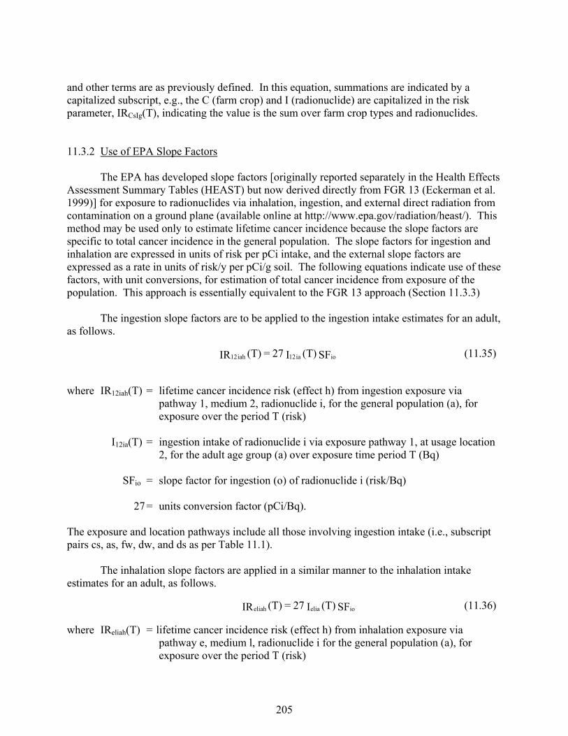
205

and other terms are as previously defined. In this equation, summations are indicated by a capitalized subscript, e.g., the C (farm crop) and I (radionuclide) are capitalized in the risk parameter, IRCsIg(T), indicating the value is the sum over farm crop types and radionuclides. 11.3.2 Use of EPA Slope Factors The EPA has developed slope factors [originally reported separately in the Health Effects Assessment Summary Tables (HEAST) but now derived directly from FGR 13 (Eckerman et al. 1999)] for exposure to radionuclides via inhalation, ingestion, and external direct radiation from contamination on a ground plane (available online at http://www.epa.gov/radiation/heast/). This method may be used only to estimate lifetime cancer incidence because the slope factors are specific to total cancer incidence in the general population. The slope factors for ingestion and inhalation are expressed in units of risk per pCi intake, and the external slope factors are expressed as a rate in units of risk/y per pCi/g soil. The following equations indicate use of these factors, with unit conversions, for estimation of total cancer incidence from exposure of the population. This approach is essentially equivalent to the FGR 13 approach (Section 11.3.3) The ingestion slope factors are to be applied to the ingestion intake estimates for an adult, as follows.

where IR12iah(T) = lifetime cancer incidence risk (effect h) from ingestion exposure via

pathway 1, medium 2, radionuclide i, for the general population (a), for exposure over the period T (risk)

I12ia(T) = ingestion intake of radionuclide i via exposure pathway 1, at usage location

2, for the adult age group (a) over exposure time period T (Bq) SFio = slope factor for ingestion (o) of radionuclide i (risk/Bq) 27 = units conversion factor (pCi/Bq). The exposure and location pathways include all those involving ingestion intake (i.e., subscript pairs cs, as, fw, dw, and ds as per Table 11.1). The inhalation slope factors are applied in a similar manner to the inhalation intake estimates for an adult, as follows.

where IReliah(T) = lifetime cancer incidence risk (effect h) from inhalation exposure via pathway e, medium l, radionuclide i for the general population (a), for exposure over the period T (risk)

SF (T)I 27 = (T)IR ioia12iah12 (11.35)

SF (T)I 27 = (T)IR ioeliaeliah (11.36)

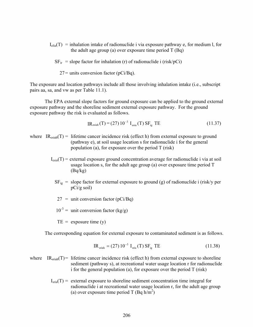
206

Ielia(T) = inhalation intake of radionuclide i via exposure pathway e, for medium l, for

the adult age group (a) over exposure time period T (Bq) SFir = slope factor for inhalation (r) of radionuclide i (risk/pCi) 27 = units conversion factor (pCi/Bq). The exposure and location pathways include all those involving inhalation intake (i.e., subscript pairs aa, sa, and vw as per Table 11.1). The EPA external slope factors for ground exposure can be applied to the ground external exposure pathway and the shoreline sediment external exposure pathway. For the ground exposure pathway the risk is evaluated as follows.

where IResiah(T) = lifetime cancer incidence risk (effect h) from external exposure to ground (pathway e), at soil usage location s for radionuclide i for the general population (a), for exposure over the period T (risk)

Iesia(T) = external exposure ground concentration average for radionuclide i via at soil

usage location s, for the adult age group (a) over exposure time period T (Bq/kg)

SFig = slope factor for external exposure to ground (g) of radionuclide i (risk/y per

pCi/g soil) 27 = unit conversion factor (pCi/Bq) 10-3 = unit conversion factor (kg/g) TE = exposure time (y) The corresponding equation for external exposure to contaminated sediment is as follows.

where IRsriah(T) = lifetime cancer incidence risk (effect h) from external exposure to shoreline sediment (pathway s), at recreational water usage location r for radionuclide i for the general population (a), for exposure over the period T (risk)

Isria(T) = external exposure to shoreline sediment concentration time integral for

radionuclide i at recreational water usage location r, for the adult age group (a) over exposure time period T (Bq h/m2)

TESF)T(I10)27( = (T)IR igesia3

esiah (11.37)

TESF)T(I10)27(IR igsria3

sriah (11.38)

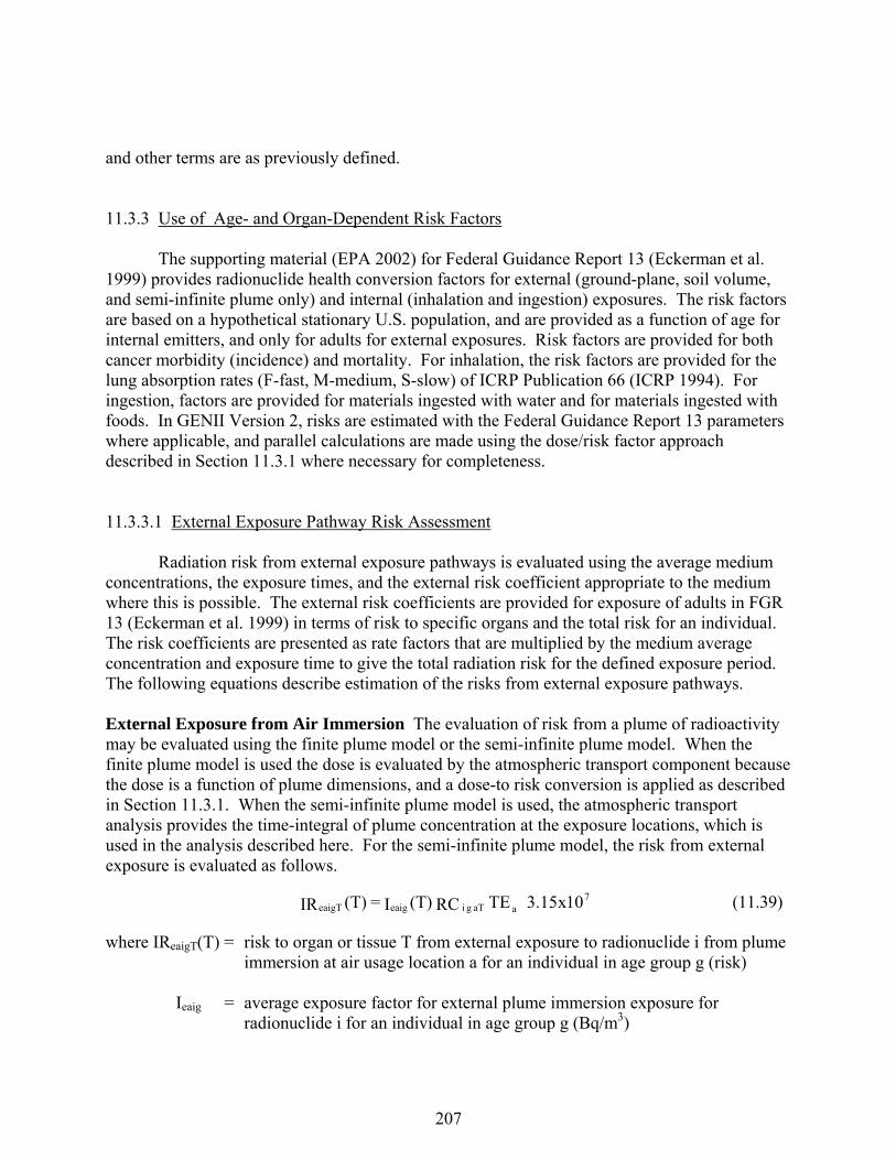
207

and other terms are as previously defined. 11.3.3 Use of Age- and Organ-Dependent Risk Factors The supporting material (EPA 2002) for Federal Guidance Report 13 (Eckerman et al. 1999) provides radionuclide health conversion factors for external (ground-plane, soil volume, and semi-infinite plume only) and internal (inhalation and ingestion) exposures. The risk factors are based on a hypothetical stationary U.S. population, and are provided as a function of age for internal emitters, and only for adults for external exposures. Risk factors are provided for both cancer morbidity (incidence) and mortality. For inhalation, the risk factors are provided for the lung absorption rates (F-fast, M-medium, S-slow) of ICRP Publication 66 (ICRP 1994). For ingestion, factors are provided for materials ingested with water and for materials ingested with foods. In GENII Version 2, risks are estimated with the Federal Guidance Report 13 parameters where applicable, and parallel calculations are made using the dose/risk factor approach described in Section 11.3.1 where necessary for completeness. 11.3.3.1 External Exposure Pathway Risk Assessment Radiation risk from external exposure pathways is evaluated using the average medium concentrations, the exposure times, and the external risk coefficient appropriate to the medium where this is possible. The external risk coefficients are provided for exposure of adults in FGR 13 (Eckerman et al. 1999) in terms of risk to specific organs and the total risk for an individual. The risk coefficients are presented as rate factors that are multiplied by the medium average concentration and exposure time to give the total radiation risk for the defined exposure period. The following equations describe estimation of the risks from external exposure pathways. External Exposure from Air Immersion The evaluation of risk from a plume of radioactivity may be evaluated using the finite plume model or the semi-infinite plume model. When the finite plume model is used the dose is evaluated by the atmospheric transport component because the dose is a function of plume dimensions, and a dose-to risk conversion is applied as described in Section 11.3.1. When the semi-infinite plume model is used, the atmospheric transport analysis provides the time-integral of plume concentration at the exposure locations, which is used in the analysis described here. For the semi-infinite plume model, the risk from external exposure is evaluated as follows.

where IReaigT(T) = risk to organ or tissue T from external exposure to radionuclide i from plume immersion at air usage location a for an individual in age group g (risk)

Ieaig = average exposure factor for external plume immersion exposure for

radionuclide i for an individual in age group g (Bq/m3)

7aaTgi eaigeaigT 10x15.3TERC (T)I = (T)IR (11.39)

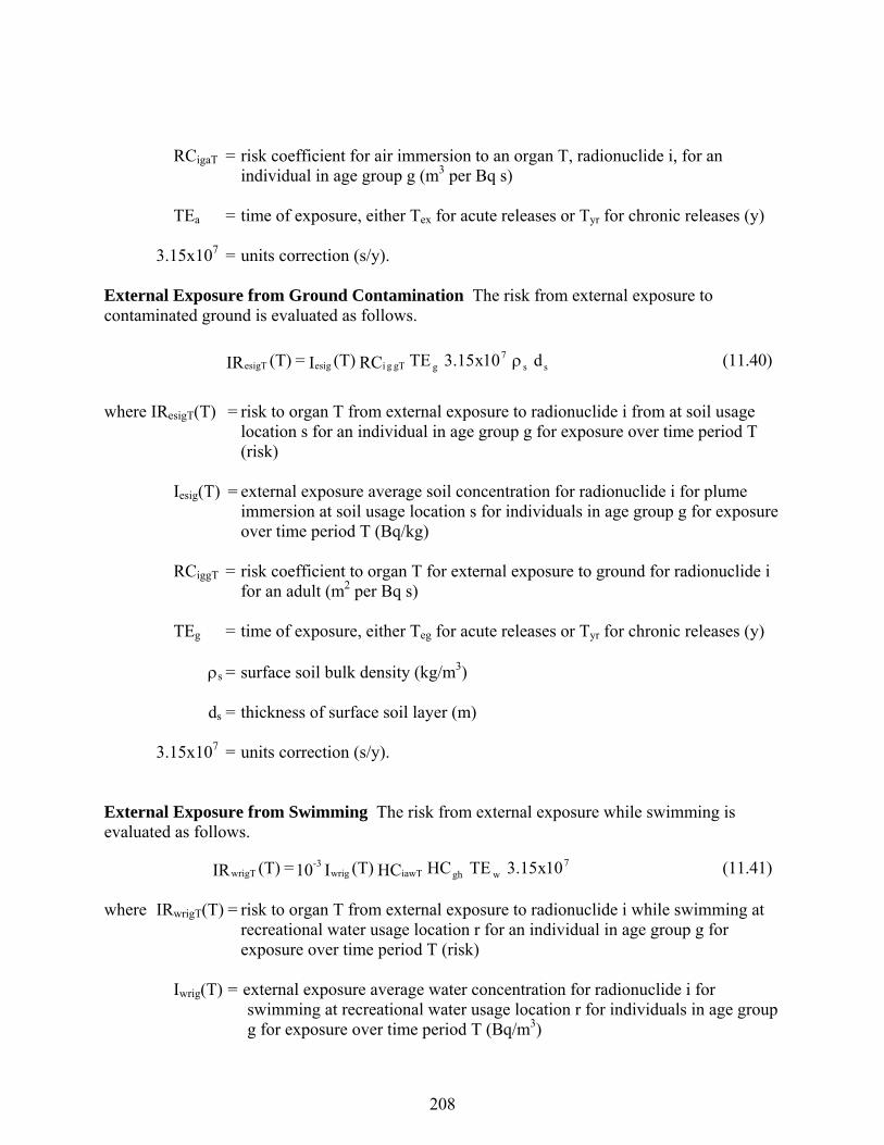
208

RCigaT = risk coefficient for air immersion to an organ T, radionuclide i, for an

individual in age group g (m3 per Bq s) TEa = time of exposure, either Tex for acute releases or Tyr for chronic releases (y) 3.15x107 = units correction (s/y). External Exposure from Ground Contamination The risk from external exposure to contaminated ground is evaluated as follows.

where IResigT(T) = risk to organ T from external exposure to radionuclide i from at soil usage location s for an individual in age group g for exposure over time period T (risk)

Iesig(T) = external exposure average soil concentration for radionuclide i for plume

immersion at soil usage location s for individuals in age group g for exposure over time period T (Bq/kg)

RCiggT = risk coefficient to organ T for external exposure to ground for radionuclide i

for an adult (m2 per Bq s) TEg = time of exposure, either Teg for acute releases or Tyr for chronic releases (y) s = surface soil bulk density (kg/m3) ds = thickness of surface soil layer (m) 3.15x107 = units correction (s/y). External Exposure from Swimming The risk from external exposure while swimming is evaluated as follows.

where IRwrigT(T) = risk to organ T from external exposure to radionuclide i while swimming at recreational water usage location r for an individual in age group g for exposure over time period T (risk)

Iwrig(T) = external exposure average water concentration for radionuclide i for

swimming at recreational water usage location r for individuals in age group g for exposure over time period T (Bq/m3)

ss7

ggTgiesigesigT d10x15.3TERC (T)I = (T)IR (11.40)

7wghiawTwrig

-3wrigT 10x15.3TEHCHC (T)I 10 = (T)IR (11.41)

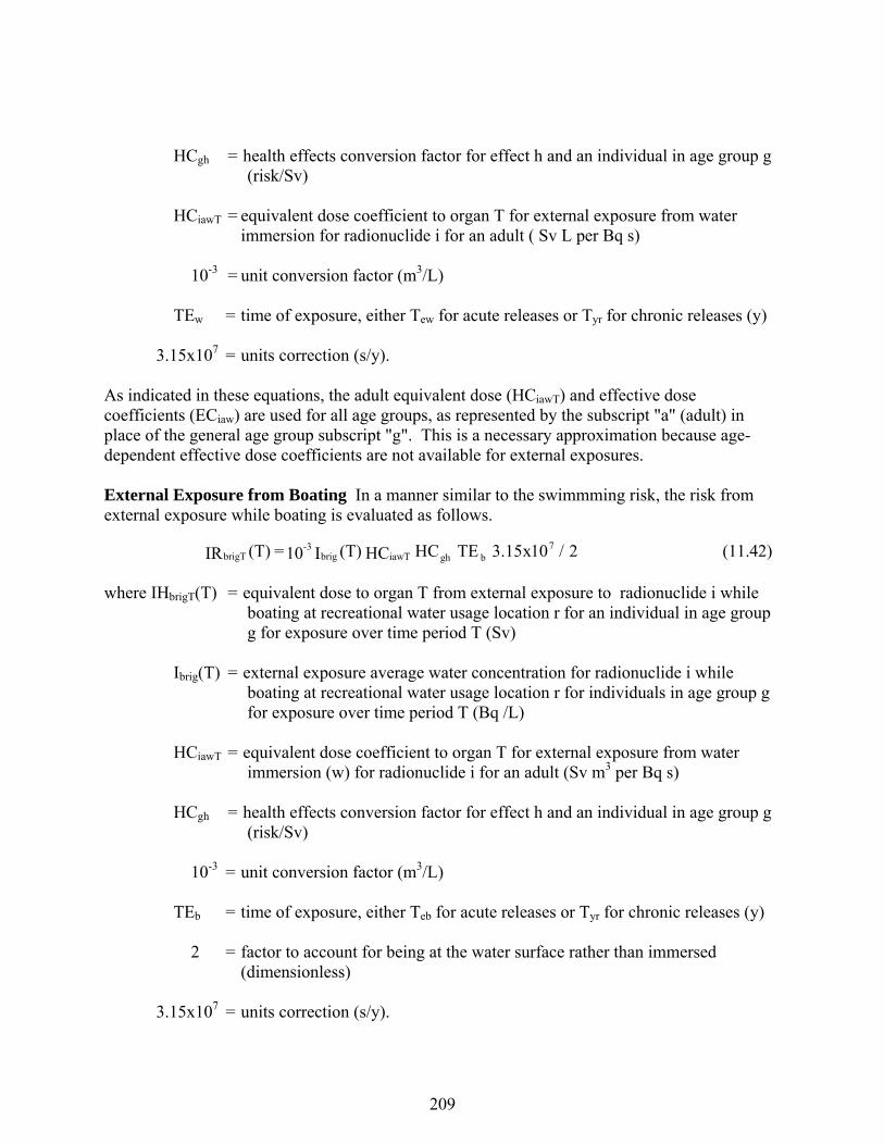
209

HCgh = health effects conversion factor for effect h and an individual in age group g

(risk/Sv) HCiawT = equivalent dose coefficient to organ T for external exposure from water

immersion for radionuclide i for an adult ( Sv L per Bq s) 10-3 = unit conversion factor (m3/L) TEw = time of exposure, either Tew for acute releases or Tyr for chronic releases (y) 3.15x107 = units correction (s/y). As indicated in these equations, the adult equivalent dose (HCiawT) and effective dose coefficients (ECiaw) are used for all age groups, as represented by the subscript "a" (adult) in place of the general age group subscript "g". This is a necessary approximation because age-dependent effective dose coefficients are not available for external exposures. External Exposure from Boating In a manner similar to the swimmming risk, the risk from external exposure while boating is evaluated as follows.

where IHbrigT(T) = equivalent dose to organ T from external exposure to radionuclide i while boating at recreational water usage location r for an individual in age group g for exposure over time period T (Sv)

Ibrig(T) = external exposure average water concentration for radionuclide i while

boating at recreational water usage location r for individuals in age group g for exposure over time period T (Bq /L)

HCiawT = equivalent dose coefficient to organ T for external exposure from water

immersion (w) for radionuclide i for an adult (Sv m3 per Bq s) HCgh = health effects conversion factor for effect h and an individual in age group g

(risk/Sv) 10-3 = unit conversion factor (m3/L) TEb = time of exposure, either Teb for acute releases or Tyr for chronic releases (y) 2 = factor to account for being at the water surface rather than immersed

(dimensionless) 3.15x107 = units correction (s/y).

2/10x15.3TEHCHC (T)I 10 = (T)IR7

bghiawTbrig-3

brigT (11.42)

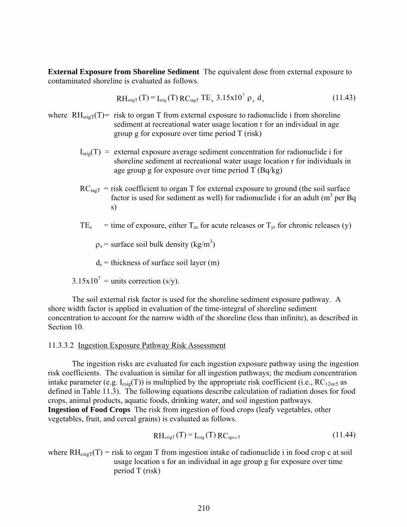
210

External Exposure from Shoreline Sediment The equivalent dose from external exposure to contaminated shoreline is evaluated as follows.

where RHsrigT(T) = risk to organ T from external exposure to radionuclide i from shoreline sediment at recreational water usage location r for an individual in age group g for exposure over time period T (risk)

Isrig(T) = external exposure average sediment concentration for radionuclide i for

shoreline sediment at recreational water usage location r for individuals in age group g for exposure over time period T (Bq/kg)

RCiagT = risk coefficient to organ T for external exposure to ground (the soil surface

factor is used for sediment as well) for radionuclide i for an adult (m3 per Bq s)

TEs = time of exposure, either Tes for acute releases or Tyr for chronic releases (y) s = surface soil bulk density (kg/m3) ds = thickness of surface soil layer (m) 3.15x107 = units correction (s/y). The soil external risk factor is used for the shoreline sediment exposure pathway. A shore width factor is applied in evaluation of the time-integral of shoreline sediment concentration to account for the narrow width of the shoreline (less than infinite), as described in Section 10. 11.3.3.2 Ingestion Exposure Pathway Risk Assessment The ingestion risks are evaluated for each ingestion exposure pathway using the ingestion risk coefficients. The evaluation is similar for all ingestion pathways; the medium concentration intake parameter (e.g. Icsig(T)) is multiplied by the appropriate risk coefficient (i.e., RC12oc5 as defined in Table 11.3). The following equations describe calculation of radiation doses for food crops, animal products, aquatic foods, drinking water, and soil ingestion pathways. Ingestion of Food Crops The risk from ingestion of food crops (leafy vegetables, other vegetables, fruit, and cereal grains) is evaluated as follows.

where RHcsigT(T) = risk to organ T from ingestion intake of radionuclide i in food crop c at soil usage location s for an individual in age group g for exposure over time period T (risk)

ss7

siagTsrigsrigT d10x15.3TERC (T)I = (T)RH (11.43)

RC (T)I = (T)RH TcigocsigcsigT (11.44)

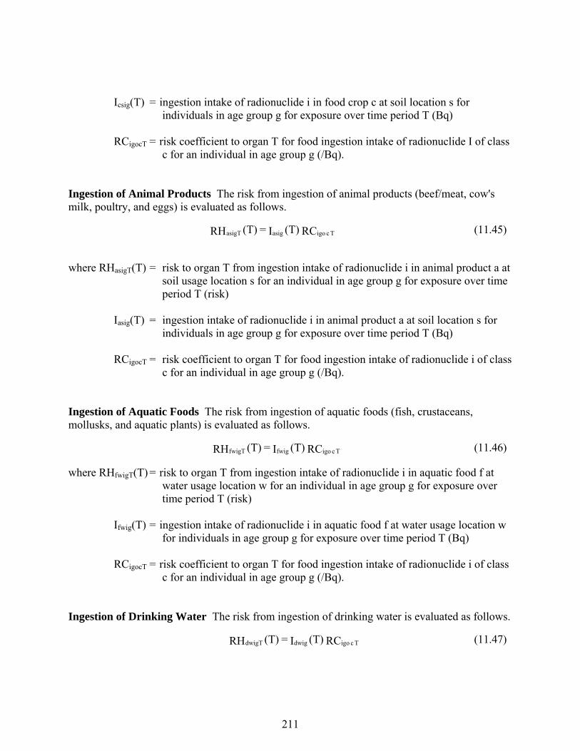
211

Icsig(T) = ingestion intake of radionuclide i in food crop c at soil location s for

individuals in age group g for exposure over time period T (Bq) RCigocT = risk coefficient to organ T for food ingestion intake of radionuclide I of class

c for an individual in age group g (/Bq). Ingestion of Animal Products The risk from ingestion of animal products (beef/meat, cow's milk, poultry, and eggs) is evaluated as follows.

where RHasigT(T) = risk to organ T from ingestion intake of radionuclide i in animal product a at

soil usage location s for an individual in age group g for exposure over time period T (risk)

Iasig(T) = ingestion intake of radionuclide i in animal product a at soil location s for

individuals in age group g for exposure over time period T (Bq) RCigocT = risk coefficient to organ T for food ingestion intake of radionuclide i of class

c for an individual in age group g (/Bq). Ingestion of Aquatic Foods The risk from ingestion of aquatic foods (fish, crustaceans, mollusks, and aquatic plants) is evaluated as follows.

where RHfwigT(T) = risk to organ T from ingestion intake of radionuclide i in aquatic food f at water usage location w for an individual in age group g for exposure over time period T (risk)

Ifwig(T) = ingestion intake of radionuclide i in aquatic food f at water usage location w

for individuals in age group g for exposure over time period T (Bq) RCigocT = risk coefficient to organ T for food ingestion intake of radionuclide i of class

c for an individual in age group g (/Bq). Ingestion of Drinking Water The risk from ingestion of drinking water is evaluated as follows.

RC (T)I = (T)RH TcigoasigasigT (11.45)

RC (T)I = (T)RH TcigofwigfwigT (11.46)

RC (T)I = (T)RH TcigodwigdwigT (11.47)

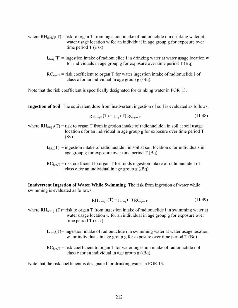
212

where RHdwigT(T) = risk to organ T from ingestion intake of radionuclide i in drinking water at water usage location w for an individual in age group g for exposure over time period T (risk)

Idwig(T) = ingestion intake of radionuclide i in drinking water at water usage location w

for individuals in age group g for exposure over time period T (Bq) RCigocT = risk coefficient to organ T for water ingestion intake of radionuclide i of

class c for an individual in age group g (/Bq). Note that the risk coefficient is specifically designated for drinking water in FGR 13. Ingestion of Soil The equivalent dose from inadvertent ingestion of soil is evaluated as follows.

where RHdsigT(T) = risk to organ T from ingestion intake of radionuclide i in soil at soil usage location s for an individual in age group g for exposure over time period T (Sv)

Idsig(T) = ingestion intake of radionuclide i in soil at soil location s for individuals in

age group g for exposure over time period T (Bq) RCigocT = risk coefficient to organ T for foods ingestion intake of radionuclide I of

class c for an individual in age group g (/Bq). Inadvertent Ingestion of Water While Swimming The risk from ingestion of water while swimming is evaluated as follows.

where RHwwigT(T)= risk to organ T from ingestion intake of radionuclide i in swimming water at water usage location w for an individual in age group g for exposure over time period T (risk)

Iwwig(T) = ingestion intake of radionuclide i in swimming water at water usage location

w for individuals in age group g for exposure over time period T (Bq) RCigocT = risk coefficient to organ T for water ingestion intake of radionuclide i of

class c for an individual in age group g (/Bq). Note that the risk coefficient is designated for drinking water in FGR 13.

RC (T)I = (T)RH TcigodsigdsigT (11.48)

RC (T)I = (T)RH TcigowigwwigTw (11.49)

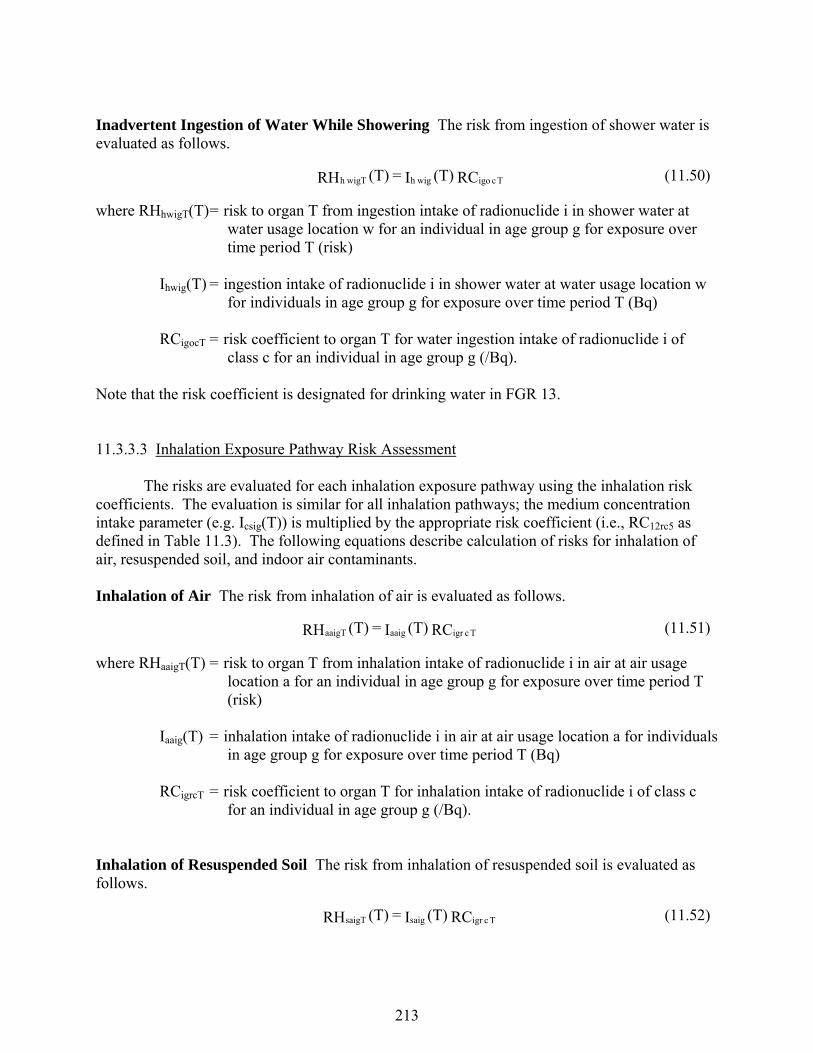
213

Inadvertent Ingestion of Water While Showering The risk from ingestion of shower water is evaluated as follows.

where RHhwigT(T) = risk to organ T from ingestion intake of radionuclide i in shower water at water usage location w for an individual in age group g for exposure over time period T (risk)

Ihwig(T) = ingestion intake of radionuclide i in shower water at water usage location w

for individuals in age group g for exposure over time period T (Bq) RCigocT = risk coefficient to organ T for water ingestion intake of radionuclide i of

class c for an individual in age group g (/Bq). Note that the risk coefficient is designated for drinking water in FGR 13. 11.3.3.3 Inhalation Exposure Pathway Risk Assessment The risks are evaluated for each inhalation exposure pathway using the inhalation risk coefficients. The evaluation is similar for all inhalation pathways; the medium concentration intake parameter (e.g. Icsig(T)) is multiplied by the appropriate risk coefficient (i.e., RC12rc5 as defined in Table 11.3). The following equations describe calculation of risks for inhalation of air, resuspended soil, and indoor air contaminants. Inhalation of Air The risk from inhalation of air is evaluated as follows.

where RHaaigT(T) = risk to organ T from inhalation intake of radionuclide i in air at air usage location a for an individual in age group g for exposure over time period T (risk)

Iaaig(T) = inhalation intake of radionuclide i in air at air usage location a for individuals

in age group g for exposure over time period T (Bq) RCigrcT = risk coefficient to organ T for inhalation intake of radionuclide i of class c

for an individual in age group g (/Bq). Inhalation of Resuspended Soil The risk from inhalation of resuspended soil is evaluated as follows.

RC (T)I = (T)RH TcigowighwigTh (11.50)

RC (T)I = (T)RH TcigraaigaaigT (11.51)

RC (T)I = (T)RH TcigrsaigsaigT (11.52)

214

where RHsaigT(T) = risk to organ T from inhalation intake of radionuclide i in resuspended soil at air usage location a for an individual in age group g for exposure over time period T (risk)

Isaig(T) = inhalation intake of radionuclide i in resuspended soil at air usage location a

for individuals in age group g for exposure over time period T (Bq) RCigrcT = risk coefficient to organ T for inhalation intake of radionuclide i of class c

for an individual in age group g (/Bq). Inhalation of Indoor Air The risk from inhalation of contaminants in indoor air is evaluated as follows.

where RHvwigT(T) = risk to organ T from inhalation intake of radionuclide i in indoor air at location w for an individual in age group g for exposure over time period T (risk)

Ivwig(T) = inhalation intake of radionuclide i in indoor air at location w for individuals

in age group g for exposure over time period T (Bq) RCigrcT = risk coefficient to organ T for inhalation intake of radionuclide i of class c

for an individual in age group g (/Bq). 11.4 REFERENCES FOR SECTION 11 Eckerman, K.F., A. B. Wolbarst, and A. C. B. Richardson. 1988. Limiting Values of Radionuclide Intake and Air Concentration and Dose Conversion Factors for Inhalation, Submersion, and Ingestion. Federal Guidance Report No. 11, EPA-520/1-88-020. U.S. Environmental Protection Agency, Washington, DC. Eckerman, K.F. and J. C. Ryman. 1993. External Exposure to Radionuclides in Air, Water, and Soil. Federal Guidance Report No. 12, EPA 402-R-93-081. U.S. Environmental Protection Agency, Washington, DC. Eckerman, K.F. R.W. Leggett, C.B. Nelson, J.S. Puskin, A.C.B. Richardson, and R.N. Stewart. 1999. Cancer Risk Coefficients for Environmental Exposure to Radionuclides, Federal Guidance Report No. 13. EPA-402-R-99-001, Office of Radiation and Indoor Air, United States Environmental Protection Agency, Washington, D.C. EPA. 1996. Radiation Exposure and Risks Assessment Manual (RERAM) Risk Assessment Using Radionuclide Slope Factors. EPA 402-R-96-016. June 1996. U.S. Environmental Protection Agency, Washington, DC.

RC (T)I = (T)RH TcigrvwigvwigT (11.53)

215

EPA. 2002. Federal Guidance Report 13, Cancer Risk Coefficients for Environmental Exposure to Radionuclides: CD Supplement, EPA-402-C-99-001, Rev. 1. United States Environmental Protection Agency, Washington, D.C. Department of Energy. 1988a. External Dose-Rate Conversion Factors for Calculation of Dose to the Public. DOE/EH-0070. U.S. Department of Energy, Washington, DC. Department of Energy. 1988b. Internal Dose Conversion Factors for Calculation of Dose to the Public. DOE/EH-0071. U.S. Department of Energy, Washington, DC. ICRP. 1989. Age-dependent Doses to Members of the Public from Intake of Radionuclides: Part 1. Annals of the ICRP. Vol. 20. No. 2 (ICRP Publication 56), Pergamon Press, New York. ICRP. 1990. "1990 Recommendations of the International Commission on Radiological Protection." Annals of the ICRP, Vol. 21, No. 1-3. Pergamon Press, New York, New York. ICRP. 1993. Age-dependent Doses to Members of the Public from Intake of Radionuclides: Part 2 Ingestion Dose Coefficients. Annals of the ICRP. Vol. 23. No. 3/4 (ICRP Publication 67), Pergamon Press, New York. ICRP. 1994. Dose Coefficients for Intakes of Radionuclides by Workers (Replacement of ICRP Publication 61). Annals of the ICRP. Vol. 24. No. 4. (ICRP Publication 68), Pergamon Press, New York. ICRP. 1995. Age-dependent Doses to Members of the Public from Intake of Radionuclides: Part 3 Ingestion Dose Coefficients. Annals of the ICRP. Vol. 25. No. 1 (ICRP Publication 69), Pergamon Press, New York. ICRP. 1995. Age-dependent Doses to Members of the Public from Intake of Radionuclides: Part 4 Inhalation Dose Coefficients. Annals of the ICRP. Vol. 25. No. 3/4 (ICRP Publication 71), Pergamon Press, New York. ICRP. 1996a. Age-dependent Doses to Members of the Public from Intake of Radionuclides: Part 5 Compilation of Ingestion and Inhalation Dose Coefficients. Annals of the ICRP. Vol. 26. No. 1 (ICRP Publication 72), Pergamon Press, New York. ICRP. 1996b. Conversion Coefficients for use in Radiological Protection against External Radiation. Annals of the ICRP. Vol 26, No.3/4 (ICRP Publication 74), Pergammon Press, New York.

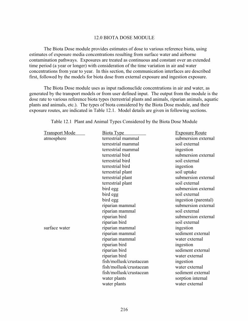
216

12.0 BIOTA DOSE MODULE

The Biota Dose module provides estimates of dose to various reference biota, using estimates of exposure media concentrations resulting from surface water and airborne contamination pathways. Exposures are treated as continuous and constant over an extended time period (a year or longer) with consideration of the time variation in air and water concentrations from year to year. In this section, the communication interfaces are described first, followed by the models for biota dose from external exposure and ingestion exposure. The Biota Dose module uses as input radionuclide concentrations in air and water, as generated by the transport models or from user defined input. The output from the module is the dose rate to various reference biota types (terrestrial plants and animals, riparian animals, aquatic plants and animals, etc.). The types of biota considered by the Biota Dose module, and their exposure routes, are indicated in Table 12.1. Model details are given in following sections. Table 12.1 Plant and Animal Types Considered by the Biota Dose Module Transport Mode Biota Type Exposure Route atmosphere terrestrial mammal submersion external terrestrial mammal soil external terrestrial mammal ingestion terrestrial bird submersion external terrestrial bird soil external terrestrial bird ingestion terrestrial plant soil uptake terrestrial plant submersion external terrestrial plant soil external bird egg submersion external bird egg soil external bird egg ingestion (parental) riparian mammal submersion external riparian mammal soil external riparian bird submersion external riparian bird soil external surface water riparian mammal ingestion riparian mammal sediment external riparian mammal water external riparian bird ingestion riparian bird sediment external riparian bird water external fish/mollusk/crustacean ingestion fish/mollusk/crustacean water external fish/mollusk/crustacean sediment external water plants sorption internal water plants water external

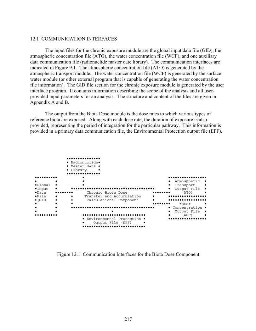
217

12.1 COMMUNICATION INTERFACES The input files for the chronic exposure module are the global input data file (GID), the atmospheric concentration file (ATO), the water concentration file (WCF), and one auxiliary data communication file (radionuclide master date library). The communication interfaces are indicated in Figure 9.1. The atmospheric concentration file (ATO) is generated by the atmospheric transport module. The water concentration file (WCF) is generated by the surface water module (or other external program that is capable of generating the water concentration file information). The GID file section for the chronic exposure module is generated by the user interface program. It contains information describing the scope of the analysis and all user-provided input parameters for an analysis. The structure and content of the files are given in Appendix A and B. The output from the Biota Dose module is the dose rates to which various types of reference biota are exposed. Along with each dose rate, the duration of exposure is also provided, representing the period of integration for the particular pathway. This information is provided in a primary data communication file, the Environmental Protection output file (EPF). ••••••••••••••• • Radionuclide• • Master Data • • Library • ••••••••••••••• •••••••••• • ••••••••••••••••• • • • • Atmospheric • •Global • • • Transport • •Input • ••••••••••••••••••••••••••••••••••••• • Output File • •Data •••••••• Chronic Biota Dose •••••••• (ATO) • •File • • Transfer and Accumulation • ••••••••••••••••• •(GID) • • Calculational Component • ••••••••••••••••• • • • •••••••• Water • • • ••••••••••••••••••••••••••••••••••••• • Concentration • • • • • Output File • •••••••••• •••••••••••••••••••••••••••• • (WCF) • • Environmental Protection • ••••••••••••••••• • Output File (EPF) • ••••••••••••••••••••••••••••

Figure 12.1 Communication Interfaces for the Biota Dose Component

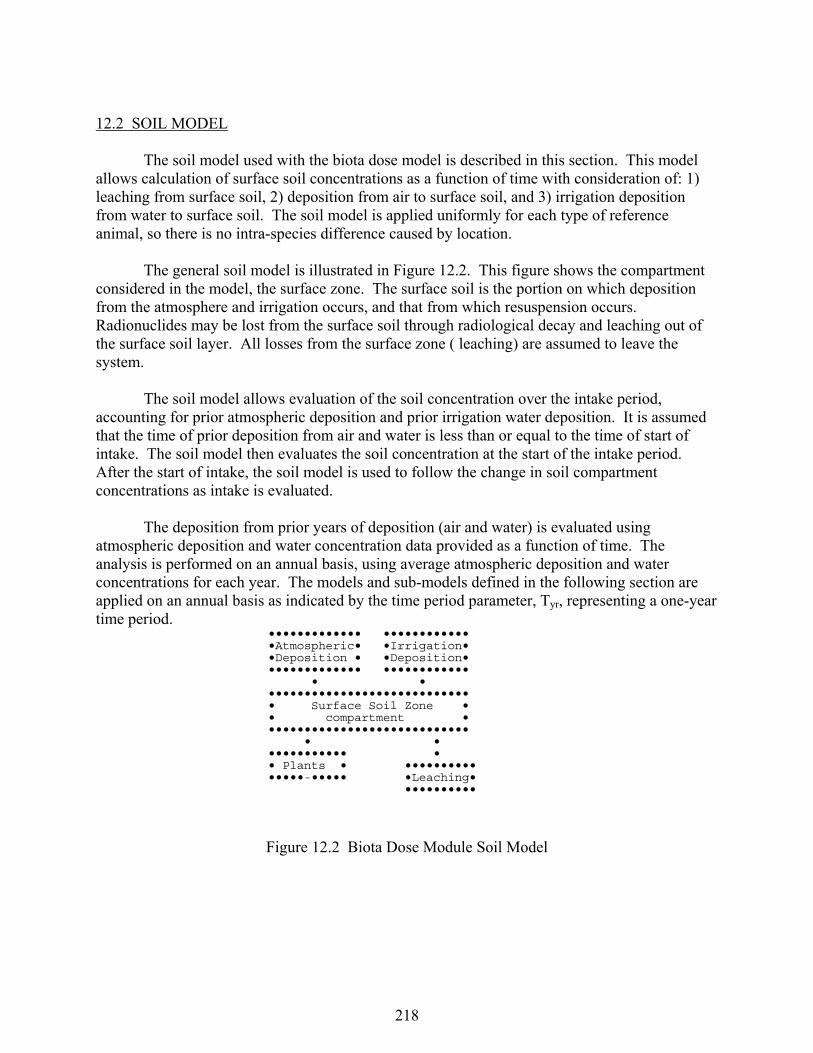
218

12.2 SOIL MODEL The soil model used with the biota dose model is described in this section. This model allows calculation of surface soil concentrations as a function of time with consideration of: 1) leaching from surface soil, 2) deposition from air to surface soil, and 3) irrigation deposition from water to surface soil. The soil model is applied uniformly for each type of reference animal, so there is no intra-species difference caused by location. The general soil model is illustrated in Figure 12.2. This figure shows the compartment considered in the model, the surface zone. The surface soil is the portion on which deposition from the atmosphere and irrigation occurs, and that from which resuspension occurs. Radionuclides may be lost from the surface soil through radiological decay and leaching out of the surface soil layer. All losses from the surface zone ( leaching) are assumed to leave the system. The soil model allows evaluation of the soil concentration over the intake period, accounting for prior atmospheric deposition and prior irrigation water deposition. It is assumed that the time of prior deposition from air and water is less than or equal to the time of start of intake. The soil model then evaluates the soil concentration at the start of the intake period. After the start of intake, the soil model is used to follow the change in soil compartment concentrations as intake is evaluated. The deposition from prior years of deposition (air and water) is evaluated using atmospheric deposition and water concentration data provided as a function of time. The analysis is performed on an annual basis, using average atmospheric deposition and water concentrations for each year. The models and sub-models defined in the following section are applied on an annual basis as indicated by the time period parameter, Tyr, representing a one-year time period. ••••••••••••• •••••••••••• •Atmospheric• •Irrigation• •Deposition • •Deposition• ••••••••••••• •••••••••••• • • •••••••••••••••••••••••••••• • Surface Soil Zone • • compartment • •••••••••••••••••••••••••••• • • ••••••••••• • • Plants • •••••••••• •••••-••••• •Leaching• ••••••••••

Figure 12.2 Biota Dose Module Soil Model

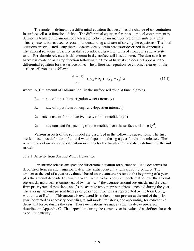
219

The model is defined by a differential equation that describes the change of concentration in surface soil as a function of time. The differential equation for the soil model compartment is defined in terms of the amount of each radionuclide chain member present in units of atoms. This representation is used for ease of understanding and ease of solving the equations. The final solutions are evaluated using the radioactive decay-chain processor described in Appendix C. The general solutions presented in that appendix are given in terms of atom units and activity units. For chronic releases, initial amount in the surface soil is set to zero. The decrease from harvest is modeled as a step function following the time of harvest and does not appear in the differential equation for the surface zone. The differential equation for chronic releases for the surface soil zone is as follows:

where Ai(t) = amount of radionuclide i in the surface soil zone at time, t (atoms) Rwi = rate of input from irrigation water (atoms /y) Rai = rate of input from atmospheric depostion (atoms/y) i = rate constant for radioactive decay of radionuclide i (y-1) Li = rate constant for leaching of radionuclide from the surface soil zone (y-1). Various aspects of the soil model are described in the following subsections. The first section describes definition of air and water deposition during a year for chronic releases. The remaining sections describe estimation methods for the transfer rate constants defined for the soil model. 12.2.1 Activity from Air and Water Deposition For chronic release analyses the differential equation for surface soil includes terms for deposition from air and irrigation water. The initial concentrations are set to be zero. The amount at the end of a year is evaluated based on the amount present at the beginning of a year plus the amount deposited during the year. In the biota exposure models that follow, the amount present during a year is composed of two terms: 1) the average amount present during the year from prior years’ depositions, and 2) the average amount present from deposited during the year. The average amount present from prior years’ contributions is represented by the term Csi(Tyr) with units of Bq/m2. This amount is evaluated from the amount present at the end of the prior year (corrected as necessary according to soil model transfers), and accounting for radioactive decay and losses during the year. These evaluations are made using the decay processor described in Appendix C. The deposition during the current year is evaluated as defined for each exposure pathway.

A ) + ( - )R + R( = td

(t)A diiLii ai

i w (12.1)

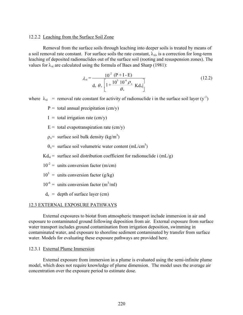
220

12.2.2 Leaching from the Surface Soil Zone Removal from the surface soils through leaching into deeper soils is treated by means of a soil removal rate constant. For surface soils the rate constant, si, is a correction for long-term leaching of deposited radionuclides out of the surface soil (rooting and resuspension zones). The values for si are calculated using the formula of Baes and Sharp (1981):

where si = removal rate constant for activity of radionuclide i in the surface soil layer (y-1) P = total annual precipitation (cm/y) I = total irrigation rate (cm/y) E = total evapotranspiration rate (cm/y) s = surface soil bulk density (kg/m3) s = surface soil volumetric water content (mL/cm3) Kdsi = surface soil distribution coefficient for radionuclide i (mL/g) 10-2 = units conversion factor (m/cm) 103 = units conversion factor (g/kg) 10-6 = units conversion factor (m3/ml) ds = depth of surface layer (cm) 12.3 EXTERNAL EXPOSURE PATHWAYS External exposures to biotat from atmospheric transport include immersion in air and exposure to contaminated ground following deposition from air. External exposure from surface water transport includes ground contamination from irrigation deposition, swimming in contaminated water, and exposure to shoreline sediment contaminated by transfer from surface water. Models for evaluating these exposure pathways are provided here. 12.3.1 External Plume Immersion External exposure from immersion in a plume is evaluated using the semi-infinite plume model, which does not require knowledge of plume dimension. The model uses the average air concentration over the exposure period to estimate dose.

Kd

10 10 + 1 d

E) - I + (P 10 =

sis

s6-3

ss

-2

si

(12.2)

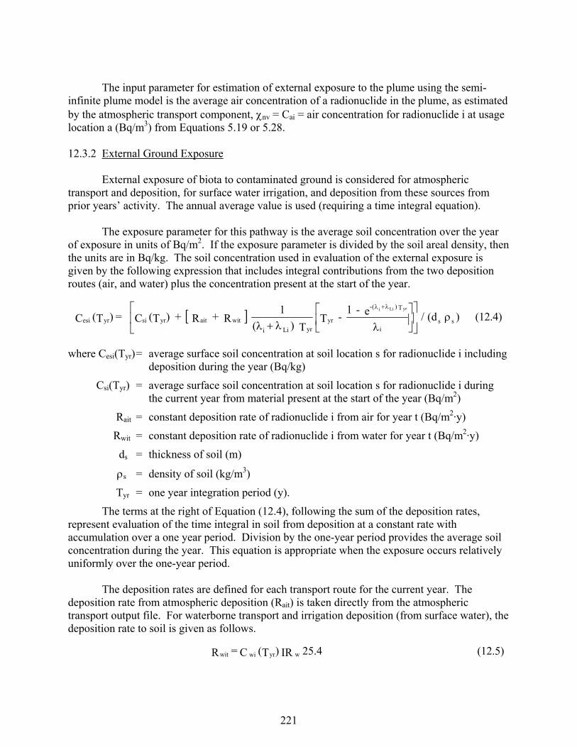
221

The input parameter for estimation of external exposure to the plume using the semi-infinite plume model is the average air concentration of a radionuclide in the plume, as estimated by the atmospheric transport component, nv = Cai = air concentration for radionuclide i at usage location a (Bq/m3) from Equations 5.19 or 5.28. 12.3.2 External Ground Exposure External exposure of biota to contaminated ground is considered for atmospheric transport and deposition, for surface water irrigation, and deposition from these sources from prior years’ activity. The annual average value is used (requiring a time integral equation). The exposure parameter for this pathway is the average soil concentration over the year of exposure in units of Bq/m2. If the exposure parameter is divided by the soil areal density, then the units are in Bq/kg. The soil concentration used in evaluation of the external exposure is given by the following expression that includes integral contributions from the two deposition routes (air, and water) plus the concentration present at the start of the year.

where Cesi(Tyr) = average surface soil concentration at soil location s for radionuclide i including deposition during the year (Bq/kg)

Csi(Tyr) = average surface soil concentration at soil location s for radionuclide i during the current year from material present at the start of the year (Bq/m2)

Rait = constant deposition rate of radionuclide i from air for year t (Bq/m2·y)

Rwit = constant deposition rate of radionuclide i from water for year t (Bq/m2·y)

ds = thickness of soil (m)

s = density of soil (kg/m3)

Tyr = one year integration period (y).

The terms at the right of Equation (12.4), following the sum of the deposition rates, represent evaluation of the time integral in soil from deposition at a constant rate with accumulation over a one year period. Division by the one-year period provides the average soil concentration during the year. This equation is appropriate when the exposure occurs relatively uniformly over the one-year period. The deposition rates are defined for each transport route for the current year. The deposition rate from atmospheric deposition (Rait) is taken directly from the atmospheric transport output file. For waterborne transport and irrigation deposition (from surface water), the deposition rate to soil is given as follows.

)d(/e - 1 - T

T )(

1 R + R + )T( C = )T( C ss

i

T ) (-

yryrLii

witaityrsiyresi

yrLii

(12.4)

25.4 IR )T( C = R wyr wiwit (12.5)

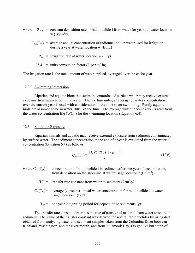
222

where Rwit = constant deposition rate of radionuclide i from water for year t at water location w (Bq/m2/y)

Cwi(Tyr) = average annual concentration of radionuclide i in water used for irrigation

during a year at water location w (Bq/L) IRw = irrigation rate at water location w (in/y) 25.4 = units conversion factor (L per m2·in) The irrigation rate is the total amount of water applied, averaged over the entire year. 12.3.3 Swimming Immersion Riparian and aquatic biota that swim in contaminated surface water may receive external exposure from immersion in the water. The the time-integral average of water concentration over the current year is used with consideration of the time spent swimming. Purely aquatic biota are assumed to be in water 100% of the time. The average water concentration is read from the water concentration file (WCF) for the swimming location (Equation 6.4). 12.3.4 Shoreline Exposure Riparian animals and aquatic may receive external exposure from sediment contaminated by surface water. The sediment concentration at the end of a year is evaluated from the water concentration (Equation 6.4) as follows.

where Csri(Tyr) = concentration of radionuclide i in sediment after one year of accumulation, from deposition on the shoreline at water usage location r (Bq/m2)

TC = transfer rate constant from water to sediment (L/m2/y) Cri(Tyr) = average (constant) annual water concentration for radionuclide i at water

usage location r (Bq/L) Tyr = one year integrating period for deposition to sediments (y). The transfer rate constant describes the rate of transfer of material from water to shoreline sediment. The value of the transfer constant was derived for several radionuclides by using data obtained from analyzing water and sediment samples taken from the Columbia River between Richland, Washington, and the river mouth, and from Tillamook Bay, Oregon, 75 km south of

i

T -yrri

yrsri

)e - (1 )T(C TC = )T(C

yri

(12.6)

223

the river mouth (Nelson 1965; Toombs and Cutler 1968). This data was analyzed by Soldat, Robinson, and Baker (1974) to derive a value of 2.54x104 in units of L/m2/y. (This is more significant figures than used in the original reference, but the original value of 102 in other units has been retained for historical consistency.) The water concentration parameter, Cri(Tyr), is provided by the waterborne transport component (Equation 6.4). The exposure is evaluated as the time-integral of shoreline sediment concentration over the current year, with consideration of the time spent on the shoreline. The external dose is evaluated by determination of the average sediment concentration during a year, as

where Csri(Tyr) = shoreline sediment time integral of exposure for radionuclide i evaluated at the usage location r (Bq/kg)

dsed = thickness of shoreline sediments (m) sed = density of shoreline sediments (kg/m3) Tyr = one year exposure period (y). For cases where there is a period of deposition during prior years but no current release, the above time integral includes consideration of decay of the accumulations from prior years, using the decay processor described in Appendix C. The time that riparian animals are not on the shoreline, they are assumed to be on nearby terrestrial soils. 12.4 TERRESTRIAL BIOTA INTERNAL CONTAMINATION Terrestrial plants may become contaminated from atmospheric fallout, irrigation, and root uptake. Terrestrial animals may become contaminated from eating terrestrial plants. The terrestrial plant is simulated as a grass. The intermediate parameter for terrestrial plants is the average concentration of radionuclides in the grass. The terrestrial plant may be contaminated by either atmospheric deposition or irrigation deposition onto plants and soil, resuspension and deposition onto plant surfaces. The plants may also be contaminated from root uptake of residual surface soil contamination. The discussion of terrestrial biota dose begins with a discussion of methods for determining the air, soil, and water concentrations that form the starting point for the calculation. The plants are then discussed, followed by the animals.

)dT(/dt (t) C = )T( C sedsedyrsri

T

0

yrsri

yr

(12.7)

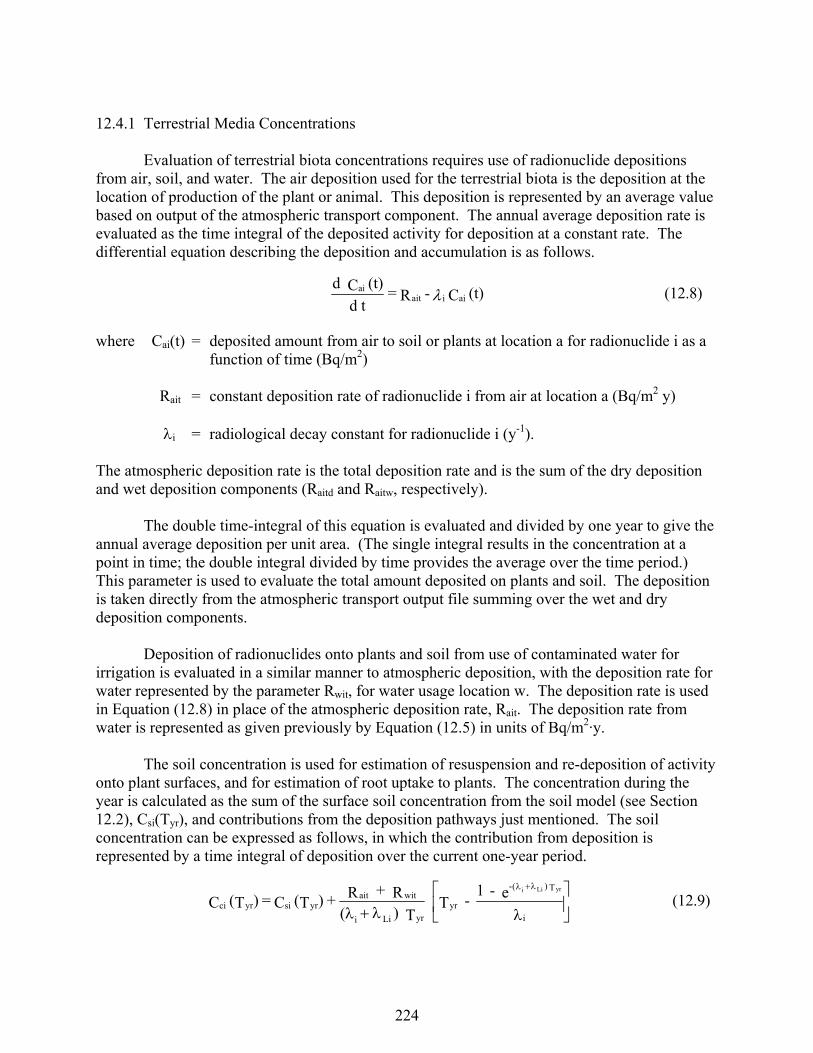
224

12.4.1 Terrestrial Media Concentrations Evaluation of terrestrial biota concentrations requires use of radionuclide depositions from air, soil, and water. The air deposition used for the terrestrial biota is the deposition at the location of production of the plant or animal. This deposition is represented by an average value based on output of the atmospheric transport component. The annual average deposition rate is evaluated as the time integral of the deposited activity for deposition at a constant rate. The differential equation describing the deposition and accumulation is as follows.

where Cai(t) = deposited amount from air to soil or plants at location a for radionuclide i as a function of time (Bq/m2)

Rait = constant deposition rate of radionuclide i from air at location a (Bq/m2 y) i = radiological decay constant for radionuclide i (y-1). The atmospheric deposition rate is the total deposition rate and is the sum of the dry deposition and wet deposition components (Raitd and Raitw, respectively). The double time-integral of this equation is evaluated and divided by one year to give the annual average deposition per unit area. (The single integral results in the concentration at a point in time; the double integral divided by time provides the average over the time period.) This parameter is used to evaluate the total amount deposited on plants and soil. The deposition is taken directly from the atmospheric transport output file summing over the wet and dry deposition components. Deposition of radionuclides onto plants and soil from use of contaminated water for irrigation is evaluated in a similar manner to atmospheric deposition, with the deposition rate for water represented by the parameter Rwit, for water usage location w. The deposition rate is used in Equation (12.8) in place of the atmospheric deposition rate, Rait. The deposition rate from water is represented as given previously by Equation (12.5) in units of Bq/m2·y. The soil concentration is used for estimation of resuspension and re-deposition of activity onto plant surfaces, and for estimation of root uptake to plants. The concentration during the year is calculated as the sum of the surface soil concentration from the soil model (see Section 12.2), Csi(Tyr), and contributions from the deposition pathways just mentioned. The soil concentration can be expressed as follows, in which the contribution from deposition is represented by a time integral of deposition over the current one-year period.

(t) C - R = td

(t) C daiiait

ai (12.8)

i

T ) (-

yryrLii

witaityrsiyrci

e - 1 - T

T )(

R + R + )T( C = )T( CyrLii

(12.9)

225

where Cci(Tyr)is the average concentration of radionuclide i in soil for plant c during the current year (Bq/m2), Csi(Tyr) is the average concentration during the current year of radionuclide i in surface soil at location s (where crop c is grown) for deposition from prior years (Bq/m2), and other terms are as previously defined. 12.4.2 Plant Concentrations The concentration in plants is evaluated as the sum of contributions from deposition onto plant surfaces, plus uptake through the roots. The contribution from deposition includes deposition directly onto plant surfaces from the air (dry and wet deposition), deposition from material resuspended from soil ,and material deposited from irrigation water. Weathering losses from plant surfaces prior to harvest is also included. The plant concentration at harvest from deposition pathways is evaluated as follows.

where Cdci(Tyr)= concentration of radionuclide i on plant c at harvest from deposition processes for a one year period (Bq/kg wet weight)

Tyr = one year exposure period (y) rdc = interception fraction from airborne dry deposition for plant type c

(dimensionless) rwc = interception fraction for airborne wet deposition to plant type c

(dimensionless) Cci(Tyr) = average concentration of radionuclide i in soil for plant type c for the current

one year period (Bq/m2) RFc = resuspension factor for crop soil (m-1) Vdi = deposition velocity of radionuclide i (m/s) 12 = months per year (mo/y) ric = interception fraction for irrigation deposition to plant type c (dimensionless),

generally equal to rwc Mc = irrigation period for plant type c (mo)

ei

3E-2.74 Tg -

c

c

c

icwitcdicyrciwcaitwdcaitdyrdci

e - 1

B

Tv

M

r 12 R + r Vd RF )T(C 7E3.15 + r R + r R = )T(C

cei

(12.10)

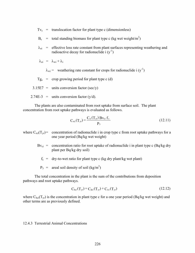
226

Tvc = translocation factor for plant type c (dimensionless) Bc = total standing biomass for plant type c (kg wet weight/m2) ei = effective loss rate constant from plant surfaces representing weathering and

radioactive decay for radionuclide i (y-1) ei = wi + i wi = weathering rate constant for crops for radionuclide i (y-1) Tgc = crop growing period for plant type c (d) 3.15E7 = units conversion factor (sec/y) 2.74E-3 = units conversion factor (y/d). The plants are also contaminated from root uptake from surface soil. The plant concentration from root uptake pathways is evaluated as follows.

where Crci(Tyr) = concentration of radionuclide i in crop type c from root uptake pathways for a one year period (Bq/kg wet weight)

Bvci = concentration ratio for root uptake of radionuclide i in plant type c (Bq/kg dry

plant per Bq/kg dry soil) fc = dry-to-wet ratio for plant type c (kg dry plant/kg wet plant) P3 = areal soil density of soil (kg/m2) The total concentration in the plant is the sum of the contributions from deposition pathways and root uptake pathways.

where Chci(Tyr) is the concentration in plant type c for a one year period (Bq/kg wet weight) and other terms are as previously defined. 12.4.3 Terrestrial Animal Concentrations

P

fBv )T(C = )T(C

3

cciyrciyrrci (12.11)

)T(C + )T(C = )T(C yrrciyrdciyrhci (12.12)

227

Pathways by which animals may become contaminated include animal ingestion of plants, water, and soil (the animals’ inhalataion is neglected as contributing little to the total). The concentration in feed plants is as defined in Equations (12.10) through (12.12). The water concentration is the value supplied on the input file, Cwi(Tyr), as the average concentration over the current year. The soil concentration is the average surface soil concentration for the year given by the parameter Cai(Tyr) for animal a, and radionuclide i in units of Bq/m2, evaluated using Equation (12.9). The concentration in an animal is evaluated as follows.

where Chai(Tyr) = concentration of radionuclide i in animal a for a one year period (Bq/kg)

Tyr = one year exposure period (y)

Fai = transfer coefficient that relates daily intake rate by an animal to the concentration in animal a (Bq/kg per Bq/d)

Cwi(Tyr) = average concentration of radionuclide i in water consumed by animals for a year (Bq/L)

Cai(Tyr) = average concentration of radionuclide i in soil consumed by animals for a year (Bq/kg dry soil)

Ccfi(Tyr) = concentration of radionuclide i in animal feed type f at time of consumption for a one year period (Bq/kg wet weight)

Uaw = daily water intake rate for animal type a (L/d)

Uas = daily soil intake rate for animal type a (kg/d)

Uaf = daily feed intake rate for animal type a of feed type f (kg/d).

12.4.3.1 Initial Interception Fraction The initial interception fraction for vegetation is a factor that accounts for the fact that not all of the material deposited within a unit area will end up on vegetation surfaces. The fraction of the total deposition that initially resides on plants is the interception fraction. Interception fractions are needed for sprinkler irrigation deposition, and for dry and wet deposition from air. The interception of material in irrigation water, ric, is not well studied. Thus, a default value of 0.25 is used for all materials deposited on all plant types by irrigation. An empirical relationship between biomass and interception fraction from atmospheric dry deposition was originally suggested by Chamberlain (1967). This model has been expanded by Pinder, Ciravolo, and Bowling (1988) for grasses. The following form of the equation is used, where the constant 2.9 is empirically derived:

U )T(C +U )T(C + U )T( C Fa = )T( C afyrcfiasyraiawyrwiiyrhai (12.13)

228

where rdc = interception fraction for atmospheric dry deposition to plant type c (dimensionless)

Bc = standing biomass of the growing vegetation for plant type c (kg wet

weight/m2) fc = dry-to-wet weight biomass ratio for plant type c (kg dry weight per kg wet

weight). The dry-to-wet ratio is required because the Pinder formulations are given in terms of dry biomass. This formulation results in the need to define the growing biomass. The interception fraction for wet deposition is evaluated as a function of the rainfall rate and standing biomass based on experimental observations of Proel and Hoffman (1993). The data by Proel and Hoffman were used to develop empirical relationships for anions, cations, and for insoluble particles. For anions, such as iodide and sulfate, the interception fraction is evaluated as follows:

where rwc = interception fraction from wet deposition to plant type c (dimensionless) Bc = standing biomass of the growing vegetation for plant type c (kg wet weight/m2) fc = dry-to-wet weight biomass ratio for plant type c (kg dry weight per kg wet

weight). R = rainfall rate (mm/d). For particles, Proel and Hoffman presented the following empirical relationship based on experiments using microspheres:

where terms are as previously defined. 12.4.3.2 Resuspension Factor The resuspension factor relates the radionuclide concentration in soil (per unit area) to the concentration in air. The resuspension factor for biota pathways is representative of conditions on agricultural land. Farmland would be expected to be tilled and have soil generally looser than soil for the general residential exposure situations.

e - 1 = r f B 2.9 -dc

cc (12.14)

R f B 2.3 = r -0.92ccwc (12.15)

R f B 2.95 = r -0.191ccwc (12.16)

229

12.4.3.3 Weathering Loss Losses from plant surfaces are represented by a weathering rate constant, wi. The rate constant is based on a weathering half time of 14 days (as used by many sources; originally derived by Soldat et al. 1974). 12.4.3.4 Soil Ingestion Terrestrial and riparian animals may ingest soil. The inadvertent ingestion of soil is evaluated for all media (atmospheric deposition to soil and surface water as a contaminated medium for irrigation). The average concentration in soil over the current one year period is evaluated as described in Section 12.2. The exposure parameter for ingestion of soil is the average soil concentration (Bq/kg soil) evaluated as follows.

where Cdsi(Tyr) = average concentration at soil location s for radionuclide i in soil consumed during the current year (Bq/kg)

Csi(Tyr) = average surface soil concentration at soil location s for radionuclide i during

the current year (Bq/m2) s = density of surface soil (g/cm3) ds = thickness of surface soil layer (cm) 104 = units conversion factor (cm2/m2) 103 = units conversion factor (g/kg) and other terms are as previously defined. The inclusion of deposition terms from air and water is evaluated for each location as appropriate to the defined exposure scenario. For example, if no irrigation is used then the irrigation deposition term, Rwit, would not be included in the calculation. 12.4.4 Aquatic Biota Aquatic biota may become contaminated when living in contaminated surface waters. The aquatic biota include fish, crustaceans, mollusks, and aquatic plants. The concentration in an aquatic denizen is based on the average surface water concentration for the current year, as follows.

i

T -

yryri

witaityrsi

ss4

3

yrdsie - 1

- T T

R + R + )T( C d 10

10 = )T( Cyri

(12.17)

230

where Chqi(Tyr)= concentration of radionuclide i in aquatic biota q (Bq/kg) Bqi = bioaccumulation factor for radionuclide i in the aquatic biota type q (Bq/kg

wet per Bq/L water). 12.5 BIOTA DOSE CALCULATIONS

The external doses are estimated based upon the following components:

Air submersion via infinite plume model based on air concentration at that location

(equivalent to the human Equation 11.4, using the infinite plume dose rate factors);

Water concentrations via whichever model is selected by the user at that location

(equivalent to the human Equation 11.7 for swimming);

Soil concentrations from aerial deposition or irrigation (equivalent to human Equation

11.5 using the infinite plane dose rate factors);

Sediment concentrations from contaminated water (equivalent to human Equation 11.11)

The internal doses are based on biota tissue concentrations calculated as described above:

Marine or freshwater aquatic plants, crustacea, mollusca, and fish are based on the

estimates of body burden estimated using water-to-fish transfer factors;

Terrestrial plants use the leafy vegetable transfer coefficient and the soil/root uptake

model parallel to “grass”;

Terrestrial mammals use the meat transfer factor and consume a diet of terrestrial plants

(essentially equivalent to an herbivore like a deer);

Riparian mammals use the meat transfer factor and consume a diet of fish (something

like a raccoon);

Terrestrial Birds use the poultry transfer factor and consume terrestrial plants (equivalent

to a type of bird like a quail or pheasant – not a raptor);

Riparian Birds use the poultry transfer factor and consume fish (a raptor);

Bird eggs use the egg transfer factor (equivalent to a medium game bird like a quail or

pheasant).

All internal dose factors come from the ERICA database calculations (Brown et al.

2008). DFs are stored in the GENII database accessed via the Constituent Database

Editor (sum of alpha, beta, and gamma components – no radiation weighting factors are

B )T(C = )T(C qiyrwiyrhqi (12.17)

231

applied; the result is straight absorbed dose). The following mapping between the

reference biota used in Brown et al. (2008) and GENII is used:

o Aquatic plant – vascular plant (marine, freshwater) o Mollusc – Benthic mollusk (marine), Bivalve mollusk (freshwater) o Crustacean – Crab (marine), Crustacean (freshwater) o Fish – Pelagic fish (marine, freshwater) o Terrestrial mammal – Large Mammal (deer) o Riparian Bird – Wading bird (duck) o Bird Egg – Bird egg (duck egg) o Terrestrial plant – Grasses and herbs (wild grass)

Doses are calculated for the exposure combinations listed in Table 12.1. Terrestrial animals are assumed to spend 100% of a year exposed to air and to upland soils. Terrestrial mammals eat grass. Riparian animals are assumed to spend 100% of a year exposed to air (if the atmospheric transport option is selected) and for input periods to riparian sediment, in addition to input periods spend immersed in water; the remaining time is spend on upland soils. Riparian animals eat fish. Aquatic biota spend 100% of a year exposed to water immersion and to underwater sediments (except for pelagic fish, for which a reduction factor of 0.5 is assumed for sediments, and for aquatic plants, which are assumed to be free-floating and not attached to the sediments). 12.6 REFERENCES FOR SECTION 12

Baes, C. F., and R. D. Sharp. 1981. Predicting Radionuclide Leaching From Root Zone Soil From Assessment Applications. CONF-81606, Oak Ridge National Laboratory, Oak Ridge, Tennessee. Brown JE, Alfonso B, Avila R, Beresford NA, Copplestone D, Prohl G, Ulanovsky A. 2008.

“The ERICA Tool”, Journal of Environmental Radioactivity 99, pp. 1371 – 1383. Chamberlain, A. C. 1967. "Transport of Lycopodium Spores and Other Small Particles to Rough Surfaces." Proc. Roy. Soc. London. A296:45-70. Nelson, J. L. 1965. "Distribution of Sediments and Associated Radionuclides in the Columbia River Below Hanford." In Hanford Radiological Sciences Research and Development Report for 1964, ed. D. W. Reece and J. K. Green, p. 3.80. USAEC Report BNWL-36, Pacific Northwest Laboratory, Richland, Washington. Pinder III, J. E., T. G. Ciravolo, and J. W. Bowling. 1988. "The Interrelationships Among Plant Biomass, Plant Surface Area, and the Interception of Particulate Deposition by Grasses." Health Phys. 55:51-58. Proel, G., and F.O. Hoffman. 1993. The Interception, Initial and Post Deposition-Retention by Vegetation of Dry and Wet Deposited Radionuclides. VAMP Terrestrial Working Group, International Atomic Energy Agency, Vienna, Austria.

232

Soldat, J. K., N. M. Robinson and D. A. Baker. 1974. Models and Computer Codes for Evaluating Environmental Radiation Doses. BNWL-1754. Battelle, Pacific Northwest Laboratory, Richland, Washington. Toombs, G. L., and P. B. Cutler, eds. 1968. Comprehensive Final Report for the Lower Columbia River Environmental Survey in Oregon, June 5, 1961 - July 31, 1967. Oregon State Board of Health, Division of Sanitation and Engineering, Salem, Oregon.

233

APPENDIX A

234

APPENDIX A: PRIMARY DATA COMMUNICATION FILE SPECIFICATIONS This appendix provides details of content and structure of each of the primary communication interface files used by the GENII-V2 software package. These files are be generated by specific components of GENII-V2, or by external programs run to interface with GENII-V2. The general structure of the primary data communication files is described first, followed by detailed information for each file. The file specifications provided here are requirements of the FRAMES software package. Primary data communication files (PDCFs) are communication interfaces between calculational components operating under the FRAMES system. The content of these files is related to radionuclide transfer rates, amounts, concentrations, intakes, or doses for particular points in the risk assessment. The content of each PDCF is dependent on the components the write and read the file. There are currently eight PDCFs defined for the GENII-V2 software package. A summary description of each is given in Table A.1, with details of each given in the following subsections. Standard file extensions are defined for each PDCF type. Table A.1 Summary Description of PDCFs

Components Involved Writing File Extension

Writing File Description

Writing File Reading File

Source Atmospheric Transport

AFF Atmospheric flux file: release rates of radionuclides to the atmosphere at the source

Source Surface Water Transport

WFF Water flux file: release rates of radionucldies to surface water at the source

Source Near-field Exposure

SCF Soil concentration file: initial concentration of radionuclides in soil (surface soil, deep soil, or waste package)

Atmospheric Transport

Acute and Chronic Exposure

ATO Air concentration file: air concentration, deposition rates, and external exposure rates to airborne radionuclides, at specific points in the environment

Surface Water Transport

Acute and Chronic Exposure

WCF Water concentration file: concentration of radionuclides in surface water at exposure location

Exposure (acute, chronic, and near-field)

Biota exposure

Receptor Intake

Environmental factors

EPF Exposure pathway file: concentration of radonuclides in exposure media

Biota doses

Receptor Intake Health Impacts RIF Receptor intake file: estimated intakes for the exposed individual

Health Impacts Report Generator HIF Health impacts file: health impact results

Report Generator HIF, others EPA Environmental Protection File: Formatted text report of results

235

A.1 GENERAL STRUCTURE OF PDCFS Each PDCF has a unique structure, defined for transmission of information between two specific components of the system. Because the PDCFs are to be used by any calculational component (not just the GENII-V2 components) to be included under the control of the Framework UI, it is necessary that the PDCF structure be compatible with many programming languages (e.g., C++ and FORTRAN). The structure of each PDCF is outlined in the following sections. These structures are subject to change as experience is gained in attempts to implement the methodology. The current descriptions are taken from the FRAMES website at http://mepas.pnl.gov/FRAMESV1/pdcf.stm A general feature of each PDCF is a heading area that is defined by each module/code developer. Information included here is variable (or nothing), however, the GENII-V2 components provide an indication of the module and transport pathways included in the analysis, as well as the date and time of the generation of the file. As with the global input data file (GID), the information in the PDCF is contained in data sets, with one set for each calculation defined for the analysis. The first line for each set contains the name of the data set and the number of lines of information that follow in the set. This line is referred to as the "marker" line. The first line of the data set (following the marker line) for a component gives the number of lines of heading information that follow. The data for the file starts in the line after the last line of heading information. The heading information may be read (or skipped) and then the data section is read. Within each PDCF structure, substructures are defined for definition of particular types of information. A minimum of one substructure is defined for each PDCF type. As an example of substructures, consider the "atmospheric transport medium" PDCF (defined below). This file provides information on the concentration in air and deposition rate to soil. Cases involving acute releases may be expected to require some information different than cases involving chronic exposures. Substructures to the PDCF are defined for acute and chronic exposures. A standard parameter identifier (e.g. "acute" or "chronic") at the start of a substructure defines the type of substructure present. A.1.2 PDCF Character and Numeric Syntax To ensure file data readability by several programming languages, the following primary standards are used for PDCFs. · The files are visually readable (ASCII/Text). · The files are readable by major programming languages (FORTRAN, C, Basic).

236

· The line syntax is compatible with FORTRAN free-field read conventions. · Each data value (string, integer, or float) is separated by a comma (,). Character fields

are fully contained within quote (') or double quote (") marks. · Floating point numbers are entered as integers, floating point values, or in scientific

notation. When PDCF files are generated by FORTRAN programs, the character fields are printed using format statements (rather that the * free-field format specification). Use of a free-field write will not properly handle character strings that have embedded commas or blanks. Quote marks and commas can easily be inserted in output lines following each parameter value (string, integer, or float), as appropriate. A.1.3 PDCF Primary Interface Parameters Each PDCF file contains information specific to the interface components involved. Some general information will always be included, such as radionuclide names and media locations. Each PDCF will also have information specific to the interface considered. The specific information is defined in Table A.2. A.1.4 Error file (ERR) An error message file (extension ERR) is to be opened by each component. If the file has not been used by the end of the run (i.e., no error messages were generated), then the file is deleted. The Framework UI will look for the file, and if present, warn the user of possible problems with the execution of that component. All executables will create the ERR file before processing is started and delete it only after all processing is complete. The file contains text information describing errors encountered during the run. The contents of the file are displayed to the user by the Framework UI. A.2 SOIL CONTAMINATION PDCF (SCF) The soil concentration file (SCF) provides information on initial radioactive contamination and gives amounts in the environmental media for subsequent exposure of individuals. The contents of the file include the following general information. · Description of source configuration (contaminated soil, landfill, etc.) · Radionuclide inventory · Release (amount or rate) of each radionuclide and decay product in soil with timing of

release as appropriate for the scenario

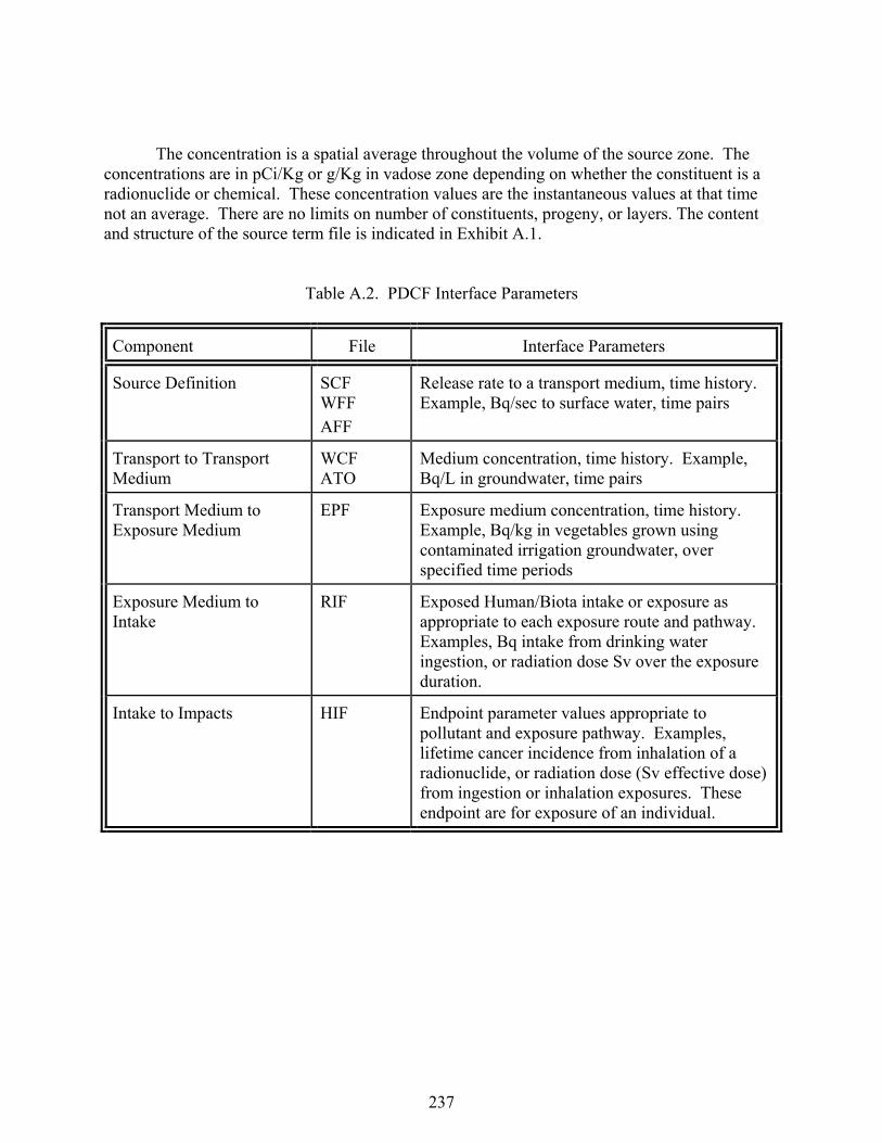
237

The concentration is a spatial average throughout the volume of the source zone. The concentrations are in pCi/Kg or g/Kg in vadose zone depending on whether the constituent is a radionuclide or chemical. These concentration values are the instantaneous values at that time not an average. There are no limits on number of constituents, progeny, or layers. The content and structure of the source term file is indicated in Exhibit A.1. Table A.2. PDCF Interface Parameters

Component File Interface Parameters

Source Definition SCF WFF AFF

Release rate to a transport medium, time history. Example, Bq/sec to surface water, time pairs

Transport to Transport Medium

WCF ATO

Medium concentration, time history. Example, Bq/L in groundwater, time pairs

Transport Medium to Exposure Medium

EPF Exposure medium concentration, time history. Example, Bq/kg in vegetables grown using contaminated irrigation groundwater, over specified time periods

Exposure Medium to Intake

RIF Exposed Human/Biota intake or exposure as appropriate to each exposure route and pathway. Examples, Bq intake from drinking water ingestion, or radiation dose Sv over the exposure duration.

Intake to Impacts HIF Endpoint parameter values appropriate to pollutant and exposure pathway. Examples, lifetime cancer incidence from inhalation of a radionuclide, or radiation dose (Sv effective dose) from ingestion or inhalation exposures. These endpoint are for exposure of an individual.

238

Exhibit A.1 Content and Structure of the SCF File For each 'Module' producing an SCF section A line with: Module Name - [STRING] Number of Lines in section - [INTEGER] End Line A line with: Number of Header Lines - [INTEGER] End Line For each 'Header Line' A line with: Header information - [STRING] End Line Next 'Header Line' A line with: Number of Data Sets - [INTEGER] End Line For each 'Data Set' A line with: Data Set name - [STRING] ;This is the location name or ID. ;If the set is intended for a particular consumming module's use then ; 'Data Set Name' = Consuming Module ID ;ElseIf the set is intended for any and all consuming modules then ; 'Data Set Name' = "All" or user may be module defined ; 'Number of Data Sets' = 1 ;EndIf Valid SCF Qualifier for this data set - [STRING] ;"Soil" / "Soil-Dissolved" / "Sediment / "Sediment-Dissolved" x Dimension of volume - [FLOAT] x Dimension unit - [Const STRING] - "m" y Dimension of volume - [FLOAT] y Dimension unit - [Const STRING] - "m" z Dimension of volume - [FLOAT] z Dimension unit - [Const STRING] - "m" Number of Constituents - [INTEGER] Centroid Easting - [FLOAT] Easting unit - [Const STRING] - "m" Centroid Northing - [FLOAT] Northing unit - [Const STRING] - "m" Centroid Depth below ground level - [FLOAT] Depth unit - [Const STRING] - "m" End Line For each 'Constituent'

239

A line with: Constituent Name - [STRING] Constituent ID - [STRING] Time unit - [Const STRING] - "yr" Concentration unit - [Const STRING] ;File qualifier determines concentration units and aids in connection scheme: ;Soil - "pCi/kg" / "mg/kg" - Total constituent mass per dry weight of soil ;Soil-Dissolved - "pCi/L" / "mg/L" - Dissolved constituent mass per volume of soil water ;Sediment - "pCi/kg" / "mg/kg" - Total constituent mass per dry weight of sediment ;Sediment-Dissolved - "pCi/L" / mg/L - Dissolved mass in water per volume of water Number of Time Concentration Pairs - [INTEGER] Number of progeny - [const INTEGER] - 0 ; must be set to zero for 1.6+ specifications End Line For each 'Time Concentration Pair' A line with: Time - [FLOAT] Constituent Concentration - [FLOAT] End Line Next 'Time Concentration Pair' Next 'Constituent' Next 'Data Set' Next 'Module' A.3 SURFACE WATER RELEASE PCDF (WFF)

The water flux file (WFF) provides the rate of transfer into a water transport medium. In the GENII V.2 software, this file is used for input to the surface water hydrology analysis (see Section 6). The flux is the rate of transfer into the surface water body defined as a function of time. The flux is a spatial average through a rectangular plane segment that is the release point to the surface water. (The physical dimensions are not used in GENII-V2, but the format is required by FRAMES.) The fluxes are in pCi/yr or g/yr depending on whether the constituent is a radionuclide or chemical. These flux values are the instantaneous values at that time, not an average. There are no limits on number of constituents, progeny, fluxes, or layers.

The content and structure of the source term file is indicated in Exhibit A.2.

Exhibit A.2 Structure and Content of the WFF File

For each 'Module' producing a WFF section A line with: Module Name - [STRING] Number of Lines in section - [INTEGER] End Line A line with:

240

Number of Header Lines - [INTEGER] End Line For each 'Header Line' A line with: Header information - [STRING] End Line Next 'Header Line' A line with: Number of Data Sets - [INTEGER] End Line For each 'Data Set' A line with: Data Set Name - [STRING] ;Intended consuming module name, use any connected consuming module name. ;If the set is intended for all consuming modules then ; 'Data Set Name' = "All" ; 'Number of Data Sets' = 1 ;EndIf Valid WFF Qualifier for this data set - [STRING] ;"Vadose" / "Aquifer" / "Surface Water" Width of flux plane - [FLOAT] Width units - [Const STRING] - "m" Length/Height of flux plane - [FLOAT] Length/Height unit - [Const STRING] - "m", Distance from Water Table - [FLOAT] ;Or the upper surface of the water body in the case of ;rivers, estuaries, etc. to Top of Flux plane. ;"0" If medium is NOT providing fluxes to the aquifer. Distance from Water Table unit - [Const STRING] - "m", Deprecated - Natural Recharge Rate - [FLOAT] Deprecated - Natural Recharge Rate unit - [Const STRING] - "m/yr" Number of Constituents - [INTEGER] End Line A line with: Water Flux Time unit - [Const STRING] - "yr" Water Flux unit - [Const STRING] - "m^3/yr" Number of Water Flux Time Pairs - [INTEGER] End Line For each 'Water Flux Time Pair' A line with: Time - [FLOAT] Water Flux - [FLOAT] End Line Next 'Water Flux Time Pair' For each 'Constituent'

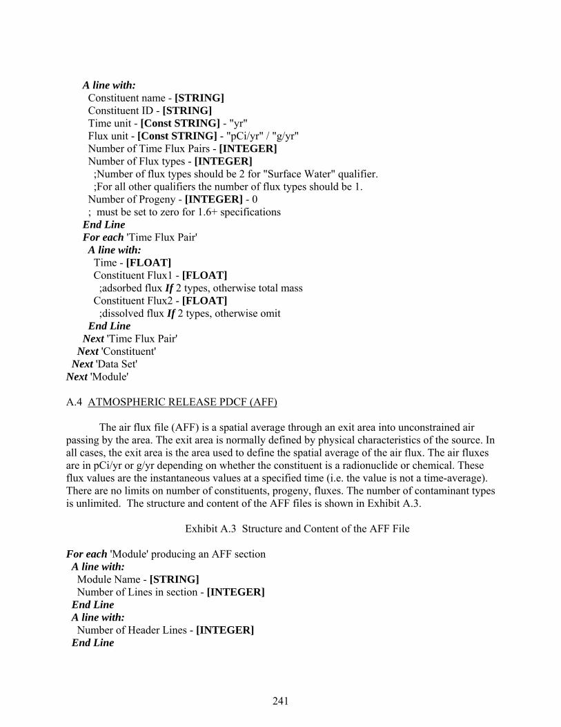
241

A line with: Constituent name - [STRING] Constituent ID - [STRING] Time unit - [Const STRING] - "yr" Flux unit - [Const STRING] - "pCi/yr" / "g/yr" Number of Time Flux Pairs - [INTEGER] Number of Flux types - [INTEGER] ;Number of flux types should be 2 for "Surface Water" qualifier. ;For all other qualifiers the number of flux types should be 1. Number of Progeny - [INTEGER] - 0 ; must be set to zero for 1.6+ specifications End Line For each 'Time Flux Pair' A line with: Time - [FLOAT] Constituent Flux1 - [FLOAT] ;adsorbed flux If 2 types, otherwise total mass Constituent Flux2 - [FLOAT] ;dissolved flux If 2 types, otherwise omit End Line Next 'Time Flux Pair' Next 'Constituent' Next 'Data Set' Next 'Module' A.4 ATMOSPHERIC RELEASE PDCF (AFF)

The air flux file (AFF) is a spatial average through an exit area into unconstrained air passing by the area. The exit area is normally defined by physical characteristics of the source. In all cases, the exit area is the area used to define the spatial average of the air flux. The air fluxes are in pCi/yr or g/yr depending on whether the constituent is a radionuclide or chemical. These flux values are the instantaneous values at a specified time (i.e. the value is not a time-average). There are no limits on number of constituents, progeny, fluxes. The number of contaminant types is unlimited. The structure and content of the AFF files is shown in Exhibit A.3.

Exhibit A.3 Structure and Content of the AFF File

For each 'Module' producing an AFF section A line with: Module Name - [STRING] Number of Lines in section - [INTEGER] End Line A line with: Number of Header Lines - [INTEGER] End Line

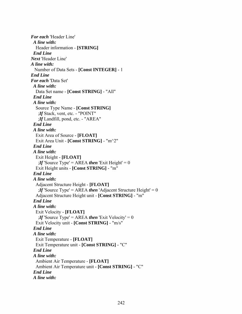
242

For each 'Header Line' A line with: Header information - [STRING] End Line Next 'Header Line' A line with: Number of Data Sets - [Const INTEGER] - 1 End Line For each 'Data Set' A line with: Data Set name - [Const STRING] - "All" End Line A line with: Source Type Name - [Const STRING] ;If Stack, vent, etc. - "POINT" ;If Landfill, pond, etc. - "AREA" End Line A line with: Exit Area of Source - [FLOAT] Exit Area Unit - [Const STRING] - "m^2" End Line A line with: Exit Height - [FLOAT] ;If 'Source Type' = AREA then 'Exit Height' = 0 Exit Height units - [Const STRING] - "m" End Line A line with: Adjacent Structure Height - [FLOAT] ;If 'Source Type' = AREA then 'Adjacent Structure Height' = 0 Adjacent Structure Height unit - [Const STRING] - "m" End Line A line with: Exit Velocity - [FLOAT] ;If 'Source Type' = AREA then 'Exit Velocity' = 0 Exit Velocity unit - [Const STRING] - "m/s" End Line A line with: Exit Temperature - [FLOAT] Exit Temperature unit - [Const STRING] - "C" End Line A line with: Ambient Air Temperature - [FLOAT] Ambient Air Temperature unit - [Const STRING] - "C" End Line A line with:

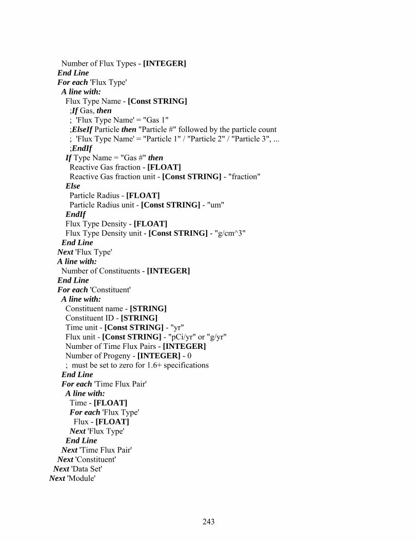
243

Number of Flux Types - [INTEGER] End Line For each 'Flux Type' A line with: Flux Type Name - [Const STRING] ;If Gas, then ; 'Flux Type Name' = "Gas 1" ;ElseIf Particle then "Particle #" followed by the particle count ; 'Flux Type Name' = "Particle 1" / "Particle 2" / "Particle 3", ... ;EndIf If Type Name = "Gas #" then Reactive Gas fraction - [FLOAT] Reactive Gas fraction unit - [Const STRING] - "fraction" Else Particle Radius - [FLOAT] Particle Radius unit - [Const STRING] - "um" EndIf Flux Type Density - [FLOAT] Flux Type Density unit - [Const STRING] - "g/cm^3" End Line Next 'Flux Type' A line with: Number of Constituents - [INTEGER] End Line For each 'Constituent' A line with: Constituent name - [STRING] Constituent ID - [STRING] Time unit - [Const STRING] - "yr" Flux unit - [Const STRING] - "pCi/yr" or "g/yr" Number of Time Flux Pairs - [INTEGER] Number of Progeny - [INTEGER] - 0 ; must be set to zero for 1.6+ specifications End Line For each 'Time Flux Pair' A line with: Time - [FLOAT] For each 'Flux Type' Flux - [FLOAT] Next 'Flux Type' End Line Next 'Time Flux Pair' Next 'Constituent' Next 'Data Set' Next 'Module'

244

A.5 TRANSPORT TO EXPOSURE The PDCFs for transport analyses contain time histories of concentrations at defined points in the environment where exposure of humans may occur. The locations are referred to as receptor locations. Two PDCFs have been identified related to transport analyses; atmospheric transport and waterborne transport (groundwater, surface water, overland transport). Descriptions of these files are provided in the following sections. A.5.1 Atmospheric Transport Output File (.ATO) The atmospheric transport output (ATO) file provides data for use by exposure pathway modules for airborne releases and atmospheric transport and deposition of pollutants. The file contents depend on options selected for the atmospheric transport analysis. The analysis may be for an acute or chronic release, or for specific exposure locations or for a grid of locations (e.g., by distance and direction). The basic data sets are provided as point values at specific locations relative to the release point. Keywords are used to define options selected. The content and structure of the ATO file is indicated in Exhibit A.4. The data in each set within the ATO file is defined according to the data set type, co-ordinate type, and receptor type defined on the second line for the data set. The program reading the information will process the information as necessary. The format of the ATO file is particularly complex. Multiple data sets can be included in one file (all related to the heading information). This allows input of acute and chronic information in one file, and use of polar co-ordinates and Cartesian co-ordinates in the same file. A.5.2 Waterborne Transport Output File (.WCF) This file provides data for use by exposure pathway modules for waterborne releases and transport. The file contains water concentrations for defined locations in the environment as a function of time. The basic data sets are provided as point values at specific locations relative to the release point. These concentration values are the instantaneous values at that time not an average at the location specified. There are no limits on number of constituents, progeny, concentrations, or receptors. The x is the easterly distance of the receptor from the source, y is the northerly, and z is the relative altitude from the source. The water concentration values concentrations are in units of pCi/ml for radionuclides. These concentration values are instantaneous values at that given time (not time averaged values). The content and structure of the WCF file is indicated in Exhibit A.5. The x is the easterly distance of the receptor from the source, y is the northerly, and z is the relative altitude from the source.

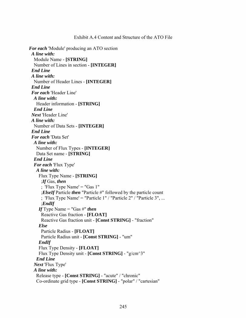
245

Exhibit A.4 Content and Structure of the ATO File For each 'Module' producing an ATO section A line with: Module Name - [STRING] Number of Lines in section - [INTEGER] End Line A line with: Number of Header Lines - [INTEGER] End Line For each 'Header Line' A line with: Header information - [STRING] End Line Next 'Header Line' A line with: Number of Data Sets - [INTEGER] End Line For each 'Data Set' A line with: Number of Flux Types - [INTEGER] Data Set name - [STRING] End Line For each 'Flux Type' A line with: Flux Type Name - [STRING] ;If Gas, then ; 'Flux Type Name' = "Gas 1" ;ElseIf Particle then "Particle #" followed by the particle count ; 'Flux Type Name' = "Particle 1" / "Particle 2" / "Particle 3", ... ;EndIf If Type Name = "Gas #" then Reactive Gas fraction - [FLOAT] Reactive Gas fraction unit - [Const STRING] - "fraction" Else Particle Radius - [FLOAT] Particle Radius unit - [Const STRING] - "um" EndIf Flux Type Density - [FLOAT] Flux Type Density unit - [Const STRING] - "g/cm^3" End Line Next 'Flux Type' A line with: Release type - [Const STRING] - "acute" / "chronic" Co-ordinate grid type - [Const STRING] - "polar" / "cartesian"

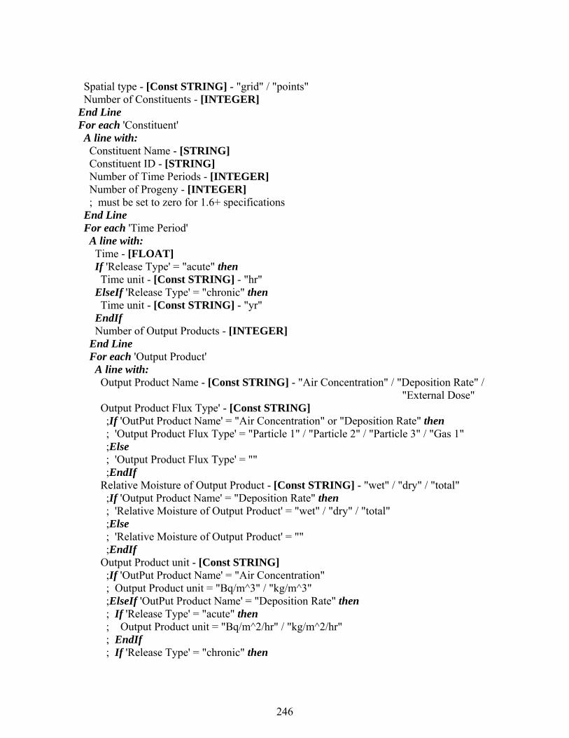
246

Spatial type - [Const STRING] - "grid" / "points" Number of Constituents - [INTEGER] End Line For each 'Constituent' A line with: Constituent Name - [STRING] Constituent ID - [STRING] Number of Time Periods - [INTEGER] Number of Progeny - [INTEGER] ; must be set to zero for 1.6+ specifications End Line For each 'Time Period' A line with: Time - [FLOAT] If 'Release Type' = "acute" then Time unit - [Const STRING] - "hr" ElseIf 'Release Type' = "chronic" then Time unit - [Const STRING] - "yr" EndIf Number of Output Products - [INTEGER] End Line For each 'Output Product' A line with: Output Product Name - [Const STRING] - "Air Concentration" / "Deposition Rate" / "External Dose" Output Product Flux Type' - [Const STRING] ;If 'OutPut Product Name' = "Air Concentration" or "Deposition Rate" then ; 'Output Product Flux Type' = "Particle 1" / "Particle 2" / "Particle 3" / "Gas 1" ;Else ; 'Output Product Flux Type' = "" ;EndIf Relative Moisture of Output Product - [Const STRING] - "wet" / "dry" / "total" ;If 'Output Product Name' = "Deposition Rate" then ; 'Relative Moisture of Output Product' = "wet" / "dry" / "total" ;Else ; 'Relative Moisture of Output Product' = "" ;EndIf Output Product unit - [Const STRING] ;If 'OutPut Product Name' = "Air Concentration" ; Output Product unit = "Bq/m^3" / "kg/m^3" ;ElseIf 'OutPut Product Name' = "Deposition Rate" then ; If 'Release Type' = "acute" then ; Output Product unit = "Bq/m^2/hr" / "kg/m^2/hr" ; EndIf ; If 'Release Type' = "chronic" then

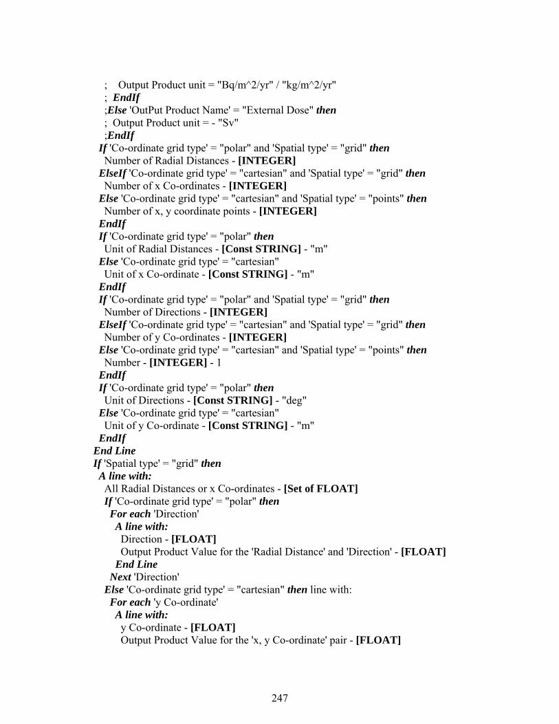
247

; Output Product unit = "Bq/m^2/yr" / "kg/m^2/yr" ; EndIf ;Else 'OutPut Product Name' = "External Dose" then ; Output Product unit = - "Sv" ;EndIf If 'Co-ordinate grid type' = "polar" and 'Spatial type' = "grid" then Number of Radial Distances - [INTEGER] ElseIf 'Co-ordinate grid type' = "cartesian" and 'Spatial type' = "grid" then Number of x Co-ordinates - [INTEGER] Else 'Co-ordinate grid type' = "cartesian" and 'Spatial type' = "points" then Number of x, y coordinate points - [INTEGER] EndIf If 'Co-ordinate grid type' = "polar" then Unit of Radial Distances - [Const STRING] - "m" Else 'Co-ordinate grid type' = "cartesian" Unit of x Co-ordinate - [Const STRING] - "m" EndIf If 'Co-ordinate grid type' = "polar" and 'Spatial type' = "grid" then Number of Directions - [INTEGER] ElseIf 'Co-ordinate grid type' = "cartesian" and 'Spatial type' = "grid" then Number of y Co-ordinates - [INTEGER] Else 'Co-ordinate grid type' = "cartesian" and 'Spatial type' = "points" then Number - [INTEGER] - 1 EndIf If 'Co-ordinate grid type' = "polar" then Unit of Directions - [Const STRING] - "deg" Else 'Co-ordinate grid type' = "cartesian" Unit of y Co-ordinate - [Const STRING] - "m" EndIf End Line If 'Spatial type' = "grid" then A line with: All Radial Distances or x Co-ordinates - [Set of FLOAT] If 'Co-ordinate grid type' = "polar" then For each 'Direction' A line with: Direction - [FLOAT] Output Product Value for the 'Radial Distance' and 'Direction' - [FLOAT] End Line Next 'Direction' Else 'Co-ordinate grid type' = "cartesian" then line with: For each 'y Co-ordinate' A line with: y Co-ordinate - [FLOAT] Output Product Value for the 'x, y Co-ordinate' pair - [FLOAT]

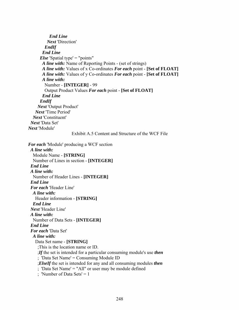
248

End Line Next 'Direction' EndIf End Line Else 'Spatial type' = "points" A line with: Name of Reporting Points - (set of strings) A line with: Values of x Co-ordinates For each point - [Set of FLOAT] A line with: Values of y Co-ordinates For each point - [Set of FLOAT] A line with: Number - [INTEGER] - 99 Output Product Values For each point - [Set of FLOAT] End Line EndIf Next 'Output Product' Next 'Time Period' Next 'Constituent' Next 'Data Set' Next 'Module'

Exhibit A.5 Content and Structure of the WCF File For each 'Module' producing a WCF section A line with: Module Name - [STRING] Number of Lines in section - [INTEGER] End Line A line with: Number of Header Lines - [INTEGER] End Line For each 'Header Line' A line with: Header information - [STRING] End Line Next 'Header Line' A line with: Number of Data Sets - [INTEGER] End Line For each 'Data Set' A line with: Data Set name - [STRING] ;This is the location name or ID. ;If the set is intended for a particular consuming module's use then ; 'Data Set Name' = Consuming Module ID ;ElseIf the set is intended for any and all consuming modules then ; 'Data Set Name' = "All" or user may be module defined ; 'Number of Data Sets' = 1

249

;EndIf Valid WCF Qualifier for this data set - [STRING] ;"Aquifer-Total" / "Aquifer" / "Surface Water-Total" / "Surface Water" Number of Constituents - [INTEGER] Measurements' Easting - [FLOAT] Easting unit - [Const STRING] - "m" Measurements' Northing - [FLOAT] Northing unit - [Const STRING] - "m" Measurements' Depth below water level - [FLOAT] Depth unit - [Const STRING] - "m" End Line For each 'Constituent' A line with: Constituent name - [STRING] Constituent ID - [STRING] Time unit - [Const STRING] - "yr" Concentration unit - [Const STRING] ;File qualifier determines concentration units and aids in connection scheme: ;Aquifer - "pCi/mL" / "g/mL" - Dissolved mass in water per volume of water ;Surface Water - "pCi/mL" / "g/mL" - Dissolved mass in water per volume of water ;Aquifer-Total - "pCi/mL" / "g/mL" - Total mass in water per volume of water ;Surface Water-Total - "pCi/mL" / "g/mL" - Total mass in water per volume of water Number of Time Concentration Pairs - [INTEGER] Number of Progeny - [const INTEGER] - 0 ; must be set to zero for 1.6+ specifications End Line For each 'Time Concentration Pair' A line with: Time - [FLOAT] Constituent Concentration - [FLOAT] End Line Next 'Time Concentration Pair' Next 'Constituent' Next 'Data Set' Next 'Module' A.6 EXPOSURE PATHWAY TO RECEPTOR INTAKE FILE (.EPF) The exposure medium component reads files providing transport medium concentrations and determines concentrations in media to which the individuals or population are exposed. The output from the exposure medium component is the concentration of each constituent in the media of interest. For external exposure pathways the output is either radiation dose (finite plume model) or time integral of medium concentration. This is the input to the intake assessment component (which produces estimates of intake and external exposure). The file extension is .EPF (exposure pathway file). Following the header information, intake information

250

is provided for all receptor locations, exposure pathways, and constituents. The content and structure of the EPF file is indicated in Exhibit A.6. Concentration units are Bq/unit medium for radionuclides. For finite plume external exposure, dose units are used, Sv. The medium concentration units are: air - m3, soil - kg or m2, water - L, foods - kg. Exhibit A.6 Content and Structure of the EPF File For each 'Module' producing an EPF section A line with: Module Name - [STRING] Number of Lines in section - [INTEGER] End Line A line with: Number of Header Lines - [INTEGER] End Line For each 'Header Line' A line with: A line with: Header information - [STRING] End Line Next 'Header Line' A line with: Number of Data Sets - [INTEGER] End Line For each 'Data Set' A line with: Data set type - [Const STRING] - "acute" / "chronic" File Extension - [STRING] ;If 'Data Set' is user defined then ; 'File Extension' is "" ;Else 'File Extension' is a valid PDCF Extension (i.e. "SCF"/ "WCF" / ...) ; The consumed PDCF's extension used to generate this data set ;EndIf ;If more than one input file was used to generate this data set then ; Separate each with a semicolon (e.g. "SCF:WCF") ;EndIf File Qualifier - [STRING] ;If 'Data Set' is user defined then ; 'File Qualifier' is the media that exposed this data set ;Else 'File Qualifier' is a valid PDCF Qualifier for 'File Extension' (i.e. "Sediment" / "Aquifer" / ...) ; The consumed PDCF's qualifier used to generate this data set ;EndIf ;If more than one input file was used to generate this data set then

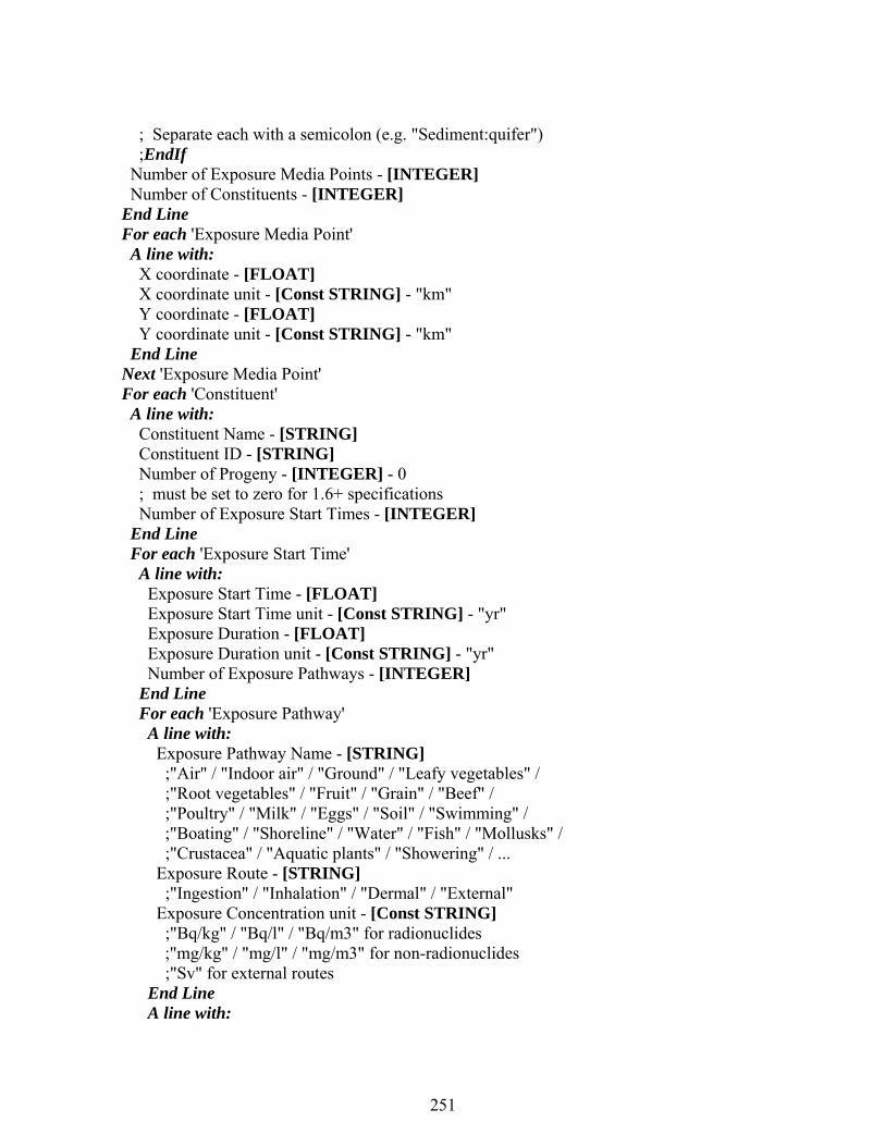
251

; Separate each with a semicolon (e.g. "Sediment:quifer") ;EndIf Number of Exposure Media Points - [INTEGER] Number of Constituents - [INTEGER] End Line For each 'Exposure Media Point' A line with: X coordinate - [FLOAT] X coordinate unit - [Const STRING] - "km" Y coordinate - [FLOAT] Y coordinate unit - [Const STRING] - "km" End Line Next 'Exposure Media Point' For each 'Constituent' A line with: Constituent Name - [STRING] Constituent ID - [STRING] Number of Progeny - [INTEGER] - 0 ; must be set to zero for 1.6+ specifications Number of Exposure Start Times - [INTEGER] End Line For each 'Exposure Start Time' A line with: Exposure Start Time - [FLOAT] Exposure Start Time unit - [Const STRING] - "yr" Exposure Duration - [FLOAT] Exposure Duration unit - [Const STRING] - "yr" Number of Exposure Pathways - [INTEGER] End Line For each 'Exposure Pathway' A line with: Exposure Pathway Name - [STRING] ;"Air" / "Indoor air" / "Ground" / "Leafy vegetables" / ;"Root vegetables" / "Fruit" / "Grain" / "Beef" / ;"Poultry" / "Milk" / "Eggs" / "Soil" / "Swimming" / ;"Boating" / "Shoreline" / "Water" / "Fish" / "Mollusks" / ;"Crustacea" / "Aquatic plants" / "Showering" / ... Exposure Route - [STRING] ;"Ingestion" / "Inhalation" / "Dermal" / "External" Exposure Concentration unit - [Const STRING] ;"Bq/kg" / "Bq/l" / "Bq/m3" for radionuclides ;"mg/kg" / "mg/l" / "mg/m3" for non-radionuclides ;"Sv" for external routes End Line A line with:

252

Exposure Concentration - [Set of FLOAT] ;a concentration For each 'Exposure Media Point' End Line Next 'Exposure Pathway' Next 'Exposure Start Time' Next 'Constituent' Next 'Data Set' Next 'Module' A.7 RECEPTOR INTAKE FILE (.RIF) The output from the receptor intake component is the intake amount for each constituent for each receptor exposure pathway. This is the input to the health impacts component (which produces estimates of health impacts, e.g., risk of developing cancer, hazard quotient, radiation dose, etc.). The input to the health impacts component is provided in this Primary Data Communication File, extension RIF (Receptor Intake File). This file provides intake amounts for each age group (as specified by the user). Following the header information, intake information is provided for all receptor locations, exposure pathways, and constituents. The content and structure of the RIF file is indicated in Exhibit A.7. Intake units are Bq for radionuclides. For external finite plume exposure, dose units are used, Sv. The number of values is equal to the number of age groups defined for the current data set. Exhibit A.7 Content and Structure of the RIF File For each 'Module' producing a RIF section A line with: Module Name - [STRING] Number of Lines in section - [INTEGER] End Line A line with: Number of Header Lines - [INTEGER] End Line For each 'Header Line' A line with: Header information - [STRING] End Line Next 'Header Line' A line with: Number of Data Sets - [INTEGER] End Line For each 'Data Set' A line with: Data set type - [Const STRING] - "acute" / "chronic"

253

File Extension - [STRING] ;If 'Data Set' is user defined then ; 'File Extension' = "" ;ElseIf 'Data Set' generated from EPF then ; 'File Extension' is passed through from EPF ;Else 'File Extension' is a valid PDCF Extension (i.e. "SCF"/ "WCF" / ...) ; The consumed PDCF's extension used to generate this data set ;EndIf ;If more than one input file was used to generate this data set then ; Separate each with a semicolon (e.g. "SCF:WCF") ;EndIf File Qualifier - [STRING] ;If 'Data Set' is user defined then ; 'File Qualifier' is the media that exposed this data set ;ElseIf 'Data Set' generated from EPF then ; 'File Qualifier' is passed through from EPF ;Else 'File Qualifier' is a valid PDCF Qualifier for 'File Extension' (i.e. "Sediment" / "Aquifer" / ...) ; The consumed PDCF's qualifier used to generate this data set ;EndIf ;If more than one input file was used to generate this data set then ; Separate each with a semicolon (e.g. "Sediment:quifer") ;EndIf Number of Exposure Media Points - [INTEGER] Number of Age Groups - [INTEGER] Number of Constituents - [INTEGER] End Line For each 'Exposure Media Point' A line with: X coordinate - [FLOAT] X coordinate unit - [Const STRING] - "km" Y coordinate - [FLOAT] Y coordinate unit - [Const STRING] - "km" End Line Next 'Exposure Media Point' For each 'Age Group' A line with: Starting Age - [FLOAT] Ending Age - [FLOAT] Age group unit - [Const STRING] - "yr" End Line For each 'Constituent' A line with: Constituent Name - [STRING] Constituent ID - [STRING]

254

Number of Progeny - [INTEGER] - 0 ; must be set to zero for 1.6+ specifications Number of Exposure Start Times - [INTEGER] End Line For each 'Exposure Start Time' A line with: Exposure Start Time - [FLOAT] Exposure Start Time unit - [Const STRING] - "yr" Exposure Duration - [FLOAT] Exposure Duration unit - [Const STRING] - "yr" Number of Exposure Pathways - [INTEGER] End Line For each 'Exposure Pathway' A line with: Exposure Pathway Population - [FLOAT] Exposure Pathway Name - [STRING] ;"Air" / "Indoor air" / "Ground" / "Leafy vegetables" / ;"Root vegetables" / "Fruit" / "Grain" / "Beef" / ;"Poultry" / "Milk" / "Eggs" / "Soil" / "Swimming" / ;"Boating" / "Shoreline" / "Water" / "Fish" / "Mollusks" / ;"Crustacea" / "Aquatic plants" / "Showering" / ... Exposure Route - [Const STRING] ;"Ingestion" / "Inhalation" / "Dermal" / "External" Exposure Intake unit - [Const STRING] ;"mg/kg/d" for non-radionuclide ingestion, dermal, inhalation routes ;"mg/m3" for non-radionuclide inhalation routes ;"Bq/kg" for radionuclide external soil routes ;"Bq/m3" for radionuclide external air routes ;"Bq/l" for radionuclide external water routes ;"Bq" for radionuclide ingestion, dermal, inhalation routes ;"Sv" for external route Exposure type - [Const STRING] ;If 'Exposure Intake unit' = "mg/kg/d" or "mg/m3" then ;"carcinogenic" / "noncarcinogenic" ;ElseIf 'Exposure Intake unit' = "Bq/kg" or "Bq/m3" or "Bq/l" then ;"concentration" ;ElseIf 'Exposure Intake unit' = "Bq" then ;"intake" ;ElseIf 'Exposure Intake unit' = "Sv" then ;"radiation dose" End Line A line with: Exposure Intake/concentration/dose - [Set of FLOAT] ;one value for each 'Exposure Media Point' End Line

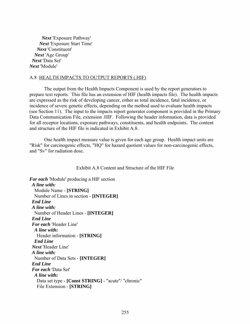
255

Next 'Exposure Pathway' Next 'Exposure Start Time' Next 'Constituent' Next 'Age Group' Next 'Data Set' Next 'Module' A.8 HEALTH IMPACTS TO OUTPUT REPORTS (.HIF) The output from the Health Impacts Component is used by the report generators to prepare text reports. This file has an extension of HIF (health impacts file). The health impacts are expressed as the risk of developing cancer, either as total incidence, fatal incidence, or incidence of severe genetic effects, depending on the method used to evaluate health impacts (see Section 11). The input to the impacts report generator component is provided in the Primary Data Communication File, extension .HIF. Following the header information, data is provided for all receptor locations, exposure pathways, constituents, and health endpoints. The content and structure of the HIF file is indicated in Exhibit A.8. One health impact measure value is given for each age group. Health impact units are "Risk" for carcinogenic effects, "HQ" for hazard quotient values for non-carcinogenic effects, and "Sv" for radiation dose. Exhibit A.8 Content and Structure of the HIF File For each 'Module' producing a HIF section A line with: Module Name - [STRING] Number of Lines in section - [INTEGER] End Line A line with: Number of Header Lines - [INTEGER] End Line For each 'Header Line' A line with: Header information - [STRING] End Line Next 'Header Line' A line with: Number of Data Sets - [INTEGER] End Line For each 'Data Set' A line with: Data set type - [Const STRING] - "acute"/ "chronic" File Extension - [STRING]

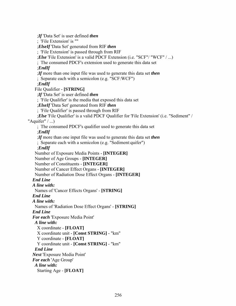
256

;If 'Data Set' is user defined then ; 'File Extension' is "" ;ElseIf 'Data Set' generated from RIF then ; 'File Extension' is passed through from RIF ;Else 'File Extension' is a valid PDCF Extension (i.e. "SCF"/ "WCF" / ...) ; The consumed PDCF's extension used to generate this data set ;EndIf ;If more than one input file was used to generate this data set then ; Separate each with a semicolon (e.g. "SCF:WCF") ;EndIf File Qualifier - [STRING] ;If 'Data Set' is user defined then ; 'File Qualifier' is the media that exposed this data set ;ElseIf 'Data Set' generated from RIF then ; 'File Qualifier' is passed through from RIF ;Else 'File Qualifier' is a valid PDCF Qualifier for 'File Extension' (i.e. "Sediment" / "Aquifer" / ...) ; The consumed PDCF's qualifier used to generate this data set ;EndIf ;If more than one input file was used to generate this data set then ; Separate each with a semicolon (e.g. "Sediment:quifer") ;EndIf Number of Exposure Media Points - [INTEGER] Number of Age Groups - [INTEGER] Number of Constituents - [INTEGER] Number of Cancer Effect Organs - [INTEGER] Number of Radiation Dose Effect Organs - [INTEGER] End Line A line with: Names of 'Cancer Effects Organs' - [STRING] End Line A line with: Names of 'Radiation Dose Effect Organs' - [STRING] End Line For each 'Exposure Media Point' A line with: X coordinate - [FLOAT] X coordinate unit - [Const STRING] - "km" Y coordinate - [FLOAT] Y coordinate unit - [Const STRING] - "km" End Line Next 'Exposure Media Point' For each 'Age Group' A line with: Starting Age - [FLOAT]

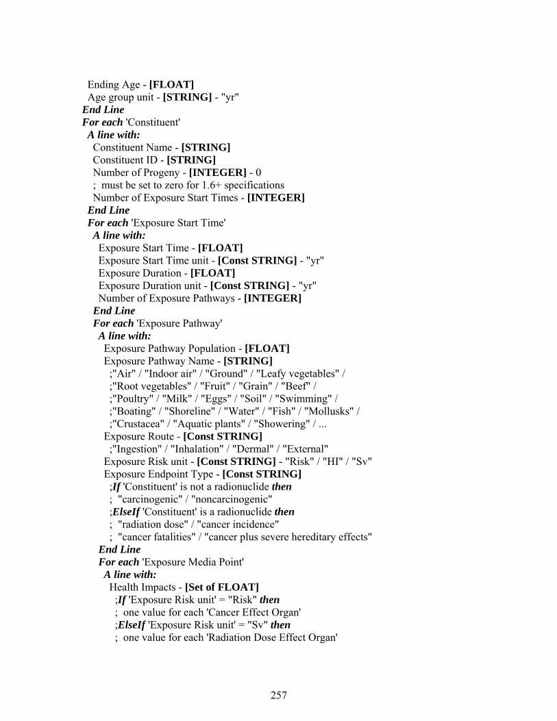
257

Ending Age - [FLOAT] Age group unit - [STRING] - "yr" End Line For each 'Constituent' A line with: Constituent Name - [STRING] Constituent ID - [STRING] Number of Progeny - [INTEGER] - 0 ; must be set to zero for 1.6+ specifications Number of Exposure Start Times - [INTEGER] End Line For each 'Exposure Start Time' A line with: Exposure Start Time - [FLOAT] Exposure Start Time unit - [Const STRING] - "yr" Exposure Duration - [FLOAT] Exposure Duration unit - [Const STRING] - "yr" Number of Exposure Pathways - [INTEGER] End Line For each 'Exposure Pathway' A line with: Exposure Pathway Population - [FLOAT] Exposure Pathway Name - [STRING] ;"Air" / "Indoor air" / "Ground" / "Leafy vegetables" / ;"Root vegetables" / "Fruit" / "Grain" / "Beef" / ;"Poultry" / "Milk" / "Eggs" / "Soil" / "Swimming" / ;"Boating" / "Shoreline" / "Water" / "Fish" / "Mollusks" / ;"Crustacea" / "Aquatic plants" / "Showering" / ... Exposure Route - [Const STRING] ;"Ingestion" / "Inhalation" / "Dermal" / "External" Exposure Risk unit - [Const STRING] - "Risk" / "HI" / "Sv" Exposure Endpoint Type - [Const STRING] ;If 'Constituent' is not a radionuclide then ; "carcinogenic" / "noncarcinogenic" ;ElseIf 'Constituent' is a radionuclide then ; "radiation dose" / "cancer incidence" ; "cancer fatalities" / "cancer plus severe hereditary effects" End Line For each 'Exposure Media Point' A line with: Health Impacts - [Set of FLOAT] ;If 'Exposure Risk unit' = "Risk" then ; one value for each 'Cancer Effect Organ' ;ElseIf 'Exposure Risk unit' = "Sv" then ; one value for each 'Radiation Dose Effect Organ'

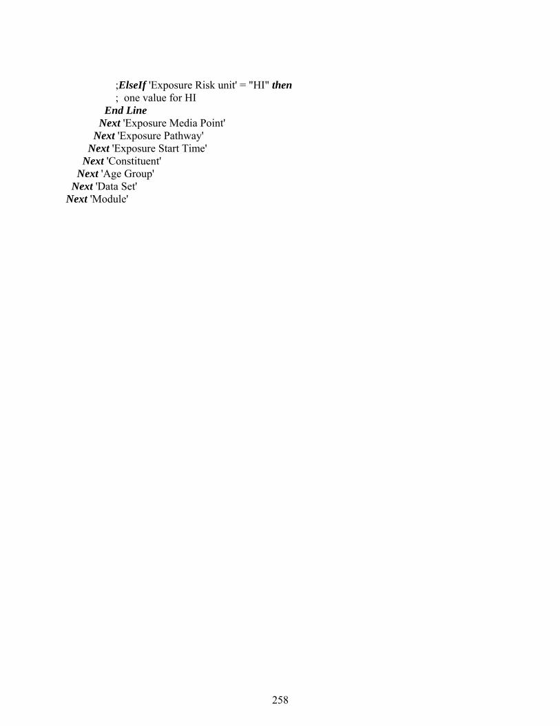
258

;ElseIf 'Exposure Risk unit' = "HI" then ; one value for HI End Line Next 'Exposure Media Point' Next 'Exposure Pathway' Next 'Exposure Start Time' Next 'Constituent' Next 'Age Group' Next 'Data Set' Next 'Module'

259

APPENDIX B

260

APPENDIX B: AUXILIARY DATA COMMUNICATION FILE SPECIFICATIONS This appendix provides detailed descriptions of content and structure of the auxiliary data communication files used by GENII-V2 modules. B.1 Radionuclide Master Data File Content The radionuclide master data library (RMDLIB.DAT) contains all radiological decay data in addition to the specification of all radionuclides for which data is included in the GENII-V2 software system. The radionuclides are organized into decay chains ordered by atomic number under the radionuclides highest in the chain. The data in this file are used by the chain decay processor to account for radioactive decay and progeny ingrowth with time. RMDLIB.DAT currently contains information on 825 radionuclides. Each parent radionuclide entry has at least 2 lines of data. If the radionuclide is the head of a decay chain, then there will be as many additional entries as there are additional members of the decay chain, one line per progeny. In some instances (primarily where the decay progeny has a very short half-life with respect to the parent), progeny are included “implicitly” – their decay energy is included with that of the parent in all applications. In these cases, the implicit progeny are included in the chain, but without indication of half-life. The first line of the file is descriptive information. The second line indicates detail about the structure of the following data: the maximum number of explicit decay progeny in a chain and the maximum number of implicit progeny in any one chain. The remaining records are set up in blocks for each parent radionuclide. This structure allows consideration of chain decay progeny and released progeny separately in the GENII-V2 calculations. The structure of the data blocks is given in Table B.1. B.2 External Radiation Dosimetry Conversion Factor Files The files F12TIII1.EXT, FGR12F32.DAT, F12TIII3.EXT, and F12TIII7.EXT contain dose rate conversion factors derived from Federal Guidance Report 12 for exposure to immersion in air, immersion in water, soil surface, and soil volume contamination, respectively. Each contains information for 825 radionuclides, and for each factors for 25 organs or tissues in the body. The files contain three lines of header information, and 828 lines of data, as illustrated in Table B.2. The file format is A7, 25E9.2. The units vary between the four files. For the air submersion , water immersion, and soil volume files, the units are Sv/s per Bq/m3. For the soil surface contamination file, the units are Sv/s per Bq/m2.

261

TABLE B.1. Radionuclide Master Library Record Structure Field Data Field Number Type Size Description Record 1: 1 CHARACTER 8 Radionuclide identifier 2 INTEGER 5 Number of explicit members in the chain 3 INTEGER 5 Number of implicit members in the chain Record 2: 1 CHARACTER 8 Radionuclide identifier (all caps) 2 REAL 13 Half-life (days) 3 INTEGER 2 Chain position number 4 INTEGER 2 Position of first parent 5 REAL 7 Branching ratio from first parent 6 INTEGER 2 Position of second parent 7 REAL 7 Branching ratio from second parent 8 INTEGER 4 Atomic mass number 9 CHARACTER 2 Bone seeker classification (not used by GENII-V2) 10 CHARACTER 1 ICRP-30 Primary lung class (not used by GENII-V2) TABLE B.2. External Dose Conversion Factor File Record Format Field Data Field Number Type Size Description 1 CHARACTER 7 Alphabetical symbol as specified in the master

radionuclide library 2-26 REAL 9 Organ-specific dose rate conversion factor. B.3 Ingestion Radiation Dosimetry Conversion Factor Files The dose conversion factors for ingestion calculated using the latest ICRP methods are provided in the file FGR13ING.GDB. This file includes significantly more data than are currently being used in GENII-V2. The file provides age-dependent radiation doses for radionuclides for various values of the gut-to-blood transfer factor (f1). The ages for which data are specified are 100 days, 1 year, 5 years, 10 years, 15 years, and 20 years. Data are provided for 33 organs, tissues, or lung compartments in the ICRP models. This information was provided by Dr. K.F. Eckerman of Oak Ridge National Laboratory. The file contains two lines of header information, followed by blocks of data for each radionuclide. For some radionuclides, information is provided for both low-LET and high-LET radiations; these radionuclides have 2 lines of data as indicated in the fourth field. The format of the information is provided in Table B.3.

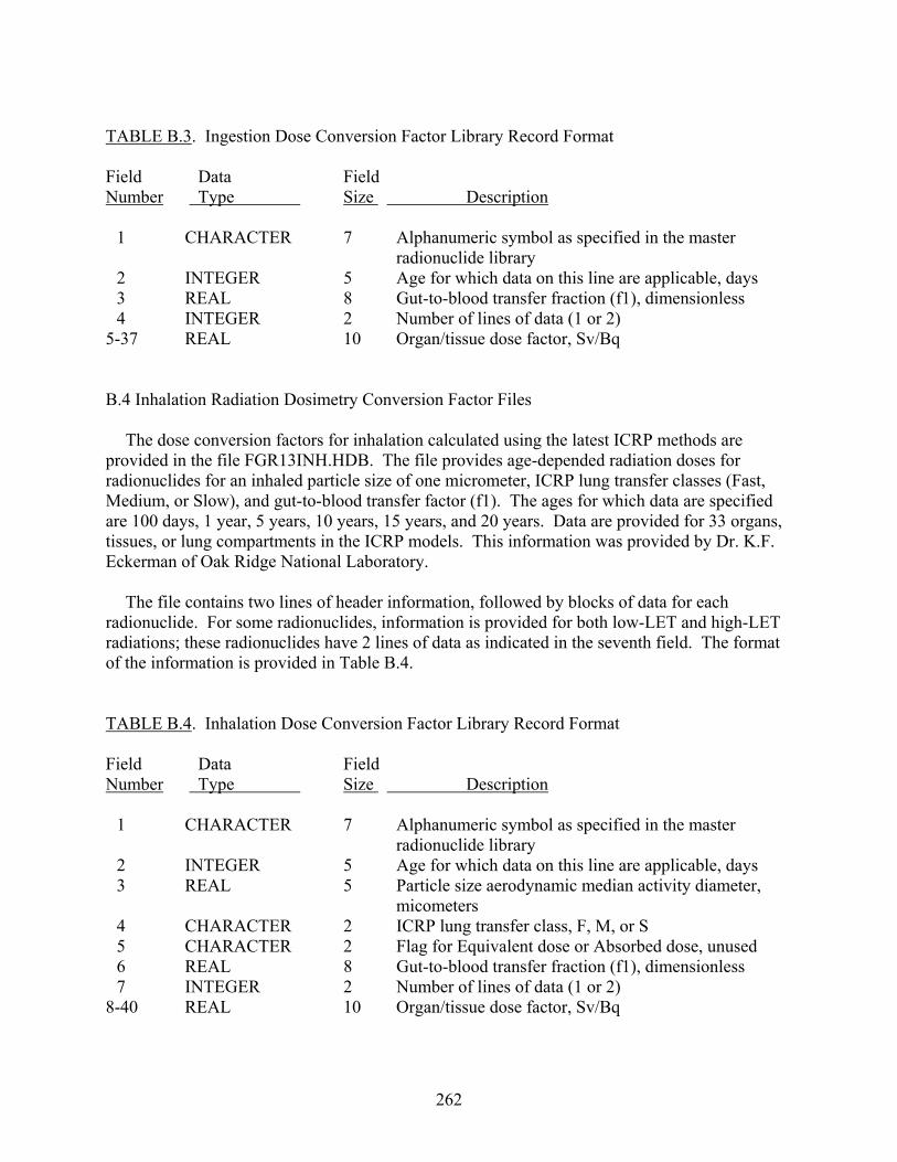
262

TABLE B.3. Ingestion Dose Conversion Factor Library Record Format Field Data Field Number Type Size Description 1 CHARACTER 7 Alphanumeric symbol as specified in the master

radionuclide library 2 INTEGER 5 Age for which data on this line are applicable, days 3 REAL 8 Gut-to-blood transfer fraction (f1), dimensionless 4 INTEGER 2 Number of lines of data (1 or 2) 5-37 REAL 10 Organ/tissue dose factor, Sv/Bq B.4 Inhalation Radiation Dosimetry Conversion Factor Files The dose conversion factors for inhalation calculated using the latest ICRP methods are provided in the file FGR13INH.HDB. The file provides age-depended radiation doses for radionuclides for an inhaled particle size of one micrometer, ICRP lung transfer classes (Fast, Medium, or Slow), and gut-to-blood transfer factor (f1). The ages for which data are specified are 100 days, 1 year, 5 years, 10 years, 15 years, and 20 years. Data are provided for 33 organs, tissues, or lung compartments in the ICRP models. This information was provided by Dr. K.F. Eckerman of Oak Ridge National Laboratory. The file contains two lines of header information, followed by blocks of data for each radionuclide. For some radionuclides, information is provided for both low-LET and high-LET radiations; these radionuclides have 2 lines of data as indicated in the seventh field. The format of the information is provided in Table B.4. TABLE B.4. Inhalation Dose Conversion Factor Library Record Format Field Data Field Number Type Size Description 1 CHARACTER 7 Alphanumeric symbol as specified in the master

radionuclide library 2 INTEGER 5 Age for which data on this line are applicable, days 3 REAL 5 Particle size aerodynamic median activity diameter,

micometers 4 CHARACTER 2 ICRP lung transfer class, F, M, or S 5 CHARACTER 2 Flag for Equivalent dose or Absorbed dose, unused 6 REAL 8 Gut-to-blood transfer fraction (f1), dimensionless 7 INTEGER 2 Number of lines of data (1 or 2) 8-40 REAL 10 Organ/tissue dose factor, Sv/Bq

263

B.5 External Radiation Risk Conversion Files The file FGR13EXT.RBS provides the risk factors for external exposure for the pathways of air submersion, soil ground plane, and soil volume sources. Data are provided for 15 cancer sites for 5 age groups. These age groups differ from those for the dose conversion factors; they are 0-5 years, 5-15, 15-25, 25-70, and lifetime. This information was provided by Dr. K.F. Eckerman of Oak Ridge National Laboratory. The file contains 3 header lines to identify and organize the material, followed by three blocks of data for each radionuclide. The format of the information is provided in Table B.5. TABLE B.5. External Risk Conversion Factor Library Record Format Field Data Field Number Type Size Description 1 CHARACTER 7 Alphanumeric symbol as specified in the master

radionuclide library 2 CHARACTER 11 Mode descriptor (air, soil surface, or soil volume) 3 CHARACTER 10 Cancer site descriptor for this line 4-8 REAL 9 Risk of mortality conversion factor for the five age

groups, risk per Bq-s 9-13 REAL 9 Risk of morbidity conversion factor for the five age

groups, risk per Bq-s 14 CHARACTER 22 Descriptor of source file for ORNL data 15 CHARACTER 10 Date of generation of data B.6 Ingestion Radiation Risk Conversion Files The file FGR13ING.RBS provides the risk factors for ingestion exposure. Data are provided for two intake pathways – drinking water and food. Information is provided on the f1 values used, but only one selection is currently available in this file for each radionuclide. Data are provided for 15 cancer sites for 5 age groups. These age groups differ from those for the dose conversion factors; they are 0-5 years, 5-15, 15-25, 25-70, and lifetime. This information was provided by Dr. K.F. Eckerman of Oak Ridge National Laboratory. The file contains 3 header lines to identify and organize the material, followed by two blocks of data for each radionuclide. The format of the information is provided in Table B.6.

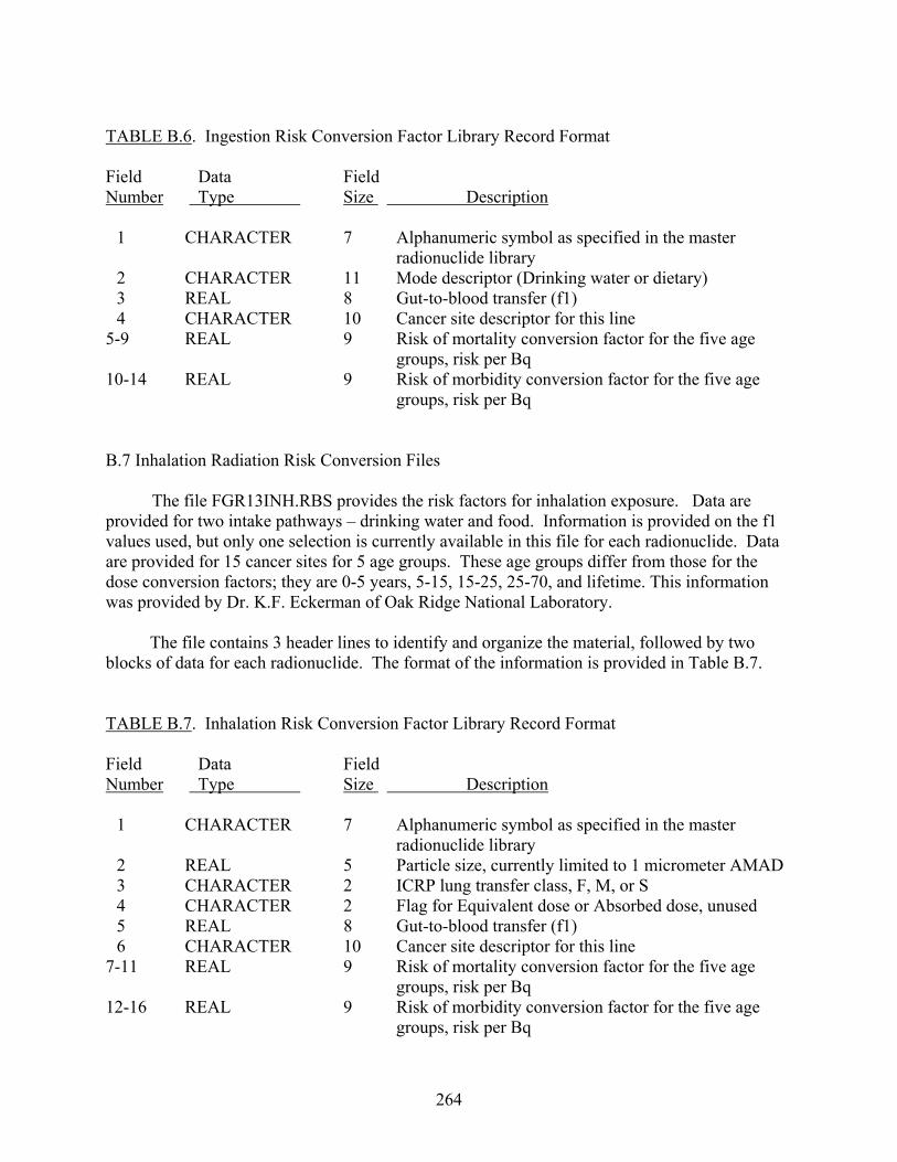
264

TABLE B.6. Ingestion Risk Conversion Factor Library Record Format Field Data Field Number Type Size Description 1 CHARACTER 7 Alphanumeric symbol as specified in the master

radionuclide library 2 CHARACTER 11 Mode descriptor (Drinking water or dietary) 3 REAL 8 Gut-to-blood transfer (f1) 4 CHARACTER 10 Cancer site descriptor for this line 5-9 REAL 9 Risk of mortality conversion factor for the five age

groups, risk per Bq 10-14 REAL 9 Risk of morbidity conversion factor for the five age

groups, risk per Bq B.7 Inhalation Radiation Risk Conversion Files The file FGR13INH.RBS provides the risk factors for inhalation exposure. Data are provided for two intake pathways – drinking water and food. Information is provided on the f1 values used, but only one selection is currently available in this file for each radionuclide. Data are provided for 15 cancer sites for 5 age groups. These age groups differ from those for the dose conversion factors; they are 0-5 years, 5-15, 15-25, 25-70, and lifetime. This information was provided by Dr. K.F. Eckerman of Oak Ridge National Laboratory. The file contains 3 header lines to identify and organize the material, followed by two blocks of data for each radionuclide. The format of the information is provided in Table B.7. TABLE B.7. Inhalation Risk Conversion Factor Library Record Format Field Data Field Number Type Size Description 1 CHARACTER 7 Alphanumeric symbol as specified in the master

radionuclide library 2 REAL 5 Particle size, currently limited to 1 micrometer AMAD 3 CHARACTER 2 ICRP lung transfer class, F, M, or S 4 CHARACTER 2 Flag for Equivalent dose or Absorbed dose, unused 5 REAL 8 Gut-to-blood transfer (f1) 6 CHARACTER 10 Cancer site descriptor for this line 7-11 REAL 9 Risk of mortality conversion factor for the five age

groups, risk per Bq 12-16 REAL 9 Risk of morbidity conversion factor for the five age

groups, risk per Bq

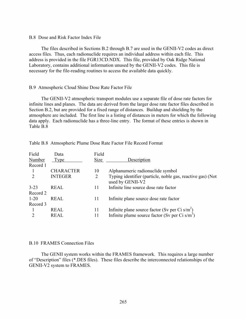
265

B.8 Dose and Risk Factor Index File The files described in Sections B.2 through B.7 are used in the GENII-V2 codes as direct access files. Thus, each radionuclide requires an individual address within each file. This address is provided in the file FGR13CD.NDX. This file, provided by Oak Ridge National Laboratory, contains additional information unused by the GENII-V2 codes. This file is necessary for the file-reading routines to access the available data quickly. B.9 Atmospheric Cloud Shine Dose Rate Factor File The GENII-V2 atmospheric transport modules use a separate file of dose rate factors for infinite lines and planes. The data are derived from the larger dose rate factor files described in Section B.2, but are provided for a fixed range of distances. Buildup and shielding by the atmosphere are included. The first line is a listing of distances in meters for which the following data apply. Each radionuclide has a three-line entry. The format of these entries is shown in Table B.8 Table B.8 Atmospheric Plume Dose Rate Factor File Record Format Field Data Field Number Type Size Description Record 1 1 CHARACTER 10 Alphanumeric radionuclide symbol 2 INTEGER 2 Typing identifier (particle, noble gas, reactive gas) (Not

used by GENII-V2 3-23 REAL 11 Infinite line source dose rate factor Record 2 1-20 REAL 11 Infinite plane source dose rate factor Record 3 1 REAL 11 Infinite plane source factor (Sv per Ci s/m2) 2 REAL 11 Infinite plume source factor (Sv per Ci s/m3) B.10 FRAMES Connection Files The GENII system works within the FRAMES framework. This requires a large number of “Description” files (*.DES files). These files describe the interconnected relationships of the GENII-V2 system to FRAMES.

266

TABLE B.9. Pseudo-code Description of DES File Contents Line with: Modeling framework check-"mf" Line with: Model Type-(string) ; "Source" ; "Air" ; "Vadose Zone" ; "Aquifer" ; "Surface Water" ; "Exposure Pathway" ; "Receptor Intake" ; "Health Impacts" ; "Viewer" ; "Import" ; "Export" ; "Closed" Module Name-(string) Module UI executable or batch path-(string) Module Model executable or batch path-(string) ; Not used in the Viewer, Import, Export, or Closed Multi-Line text string description of model ; A description of what the model is typically used for and any limiting assumptions (such as only does radionuclides, can only do 20 contaminants at a time) Typical time scale of runs - Reference to formulation documents - Reference to verification documents if they exist - Reference to validation documents if they exist - Hardware requirements - Contact point for question regarding the model

267

APPENDIX C

268

APPENDIX C: RADIOLOGICAL CHAIN-DECAY PROCESSOR A general solution to first-order compartmental models is presented in this appendix for application to systems consisting of one physical medium that contains any number of radionuclide decay chain members. The solution can be applied to any such system involving physical transfers from the medium and radioactive chain decay with branching. The general analytical solution to the problem is described mathematically and extended to evaluation of the time integral of the radionuclide quantities and to cases involving deposition from outside sources. For deposition at a constant rate during a time period, the general solution can be applied to determine the quantity present during the time period and the time integral of the quantity during the time period. Various methods have been described for evaluating systems involving radioactive decay (Bateman 1910; Friedlander and Kennedy 1955; Hamawi 1971; Scherpelz and Desrosiers 1980) and physical transfers between media (Gear 1971; Skrable et al. 1974; Hindmarsh 1983; Birchall and James 1989; Kirchner 1990). Some of these methods involve simple analytical solutions, such as the Bateman (1910) representation of the radioactive decay process without branching; others involve advanced numerical methods to solve multi-compartment systems such as the numerical differential equation solvers of Gear (1971) and Hindmarsh (1983) and the numerical matrix method described by Birchall and James (1989). The analytical solutions presented by Bateman (1910), Scherpelz and Desrosiers (1980), and Skrable et al. (1974) do not consider branching, but can account for branching by performing multiple applications of the equations to each possible decay path and summing the results appropriately, a method suggested by Friedlander and Kennedy (1955). The general solution presented in this paper includes chain decay with branching explicitly in the equations (Kennedy and Strenge 1992). The general radioactive-decay-chain problem is illustrated in Figure 1. In this figure each box represents a radionuclide decay chain member in a medium. Two types of transfers may be represented: radioactive decay between chain members and physical transfer from the medium. Radioactive transitions in this system are represented as flowing from upper boxes to lower boxes; any upper box may contribute material to any lower box. Because radioactive transitions within decay chains are irreversible, upward transfers, representing recycling of material, are not considered. Physical transfers out of the medium are indicated by the downward arrows from each box.

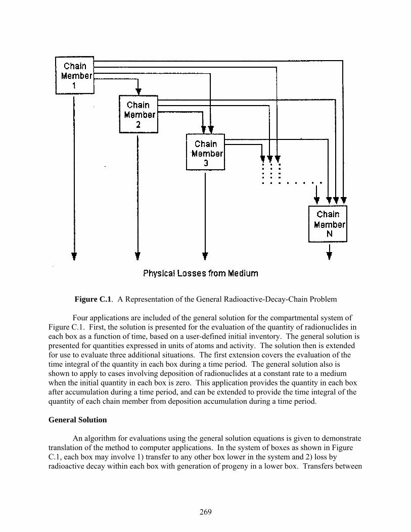
269

Four applications are included of the general solution for the compartmental system of Figure C.1. First, the solution is presented for the evaluation of the quantity of radionuclides in each box as a function of time, based on a user-defined initial inventory. The general solution is presented for quantities expressed in units of atoms and activity. The solution then is extended for use to evaluate three additional situations. The first extension covers the evaluation of the time integral of the quantity in each box during a time period. The general solution also is shown to apply to cases involving deposition of radionuclides at a constant rate to a medium when the initial quantity in each box is zero. This application provides the quantity in each box after accumulation during a time period, and can be extended to provide the time integral of the quantity of each chain member from deposition accumulation during a time period. General Solution An algorithm for evaluations using the general solution equations is given to demonstrate translation of the method to computer applications. In the system of boxes as shown in Figure C.1, each box may involve 1) transfer to any other box lower in the system and 2) loss by radioactive decay within each box with generation of progeny in a lower box. Transfers between

Figure C.1. A Representation of the General Radioactive-Decay-Chain Problem

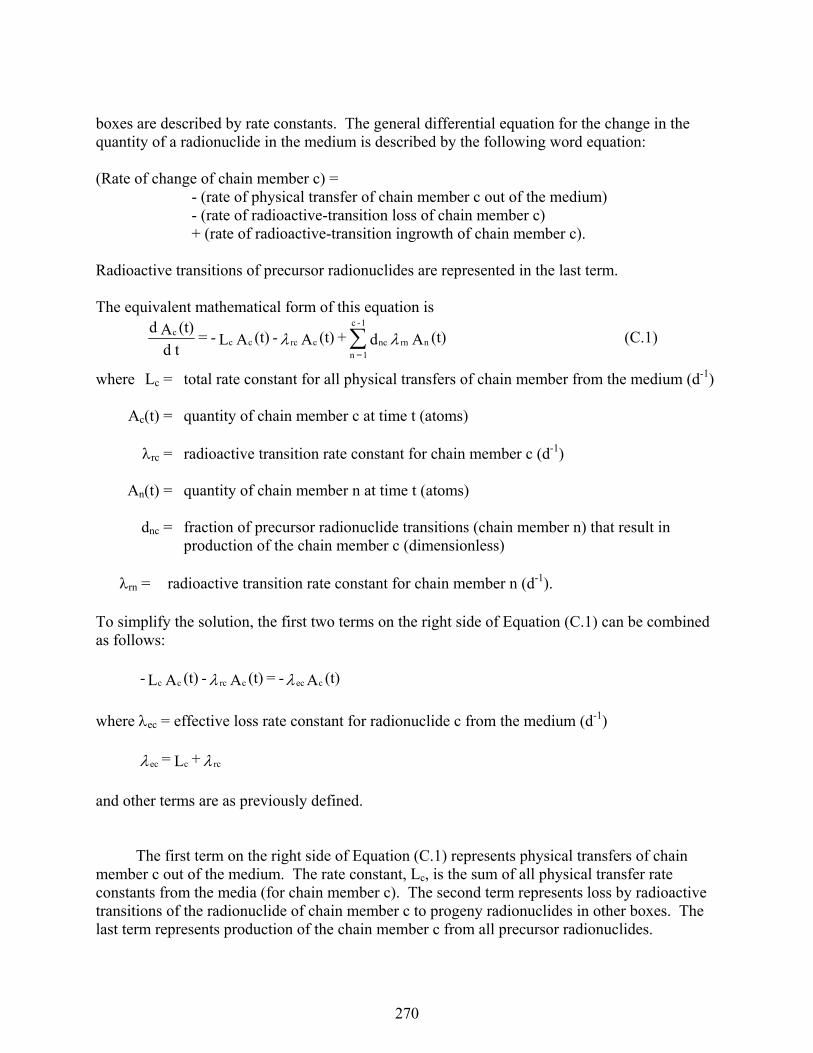
270

boxes are described by rate constants. The general differential equation for the change in the quantity of a radionuclide in the medium is described by the following word equation: (Rate of change of chain member c) = - (rate of physical transfer of chain member c out of the medium) - (rate of radioactive-transition loss of chain member c) + (rate of radioactive-transition ingrowth of chain member c). Radioactive transitions of precursor radionuclides are represented in the last term. The equivalent mathematical form of this equation is

where Lc = total rate constant for all physical transfers of chain member from the medium (d-1) Ac(t) = quantity of chain member c at time t (atoms) rc = radioactive transition rate constant for chain member c (d-1) An(t) = quantity of chain member n at time t (atoms) dnc = fraction of precursor radionuclide transitions (chain member n) that result in

production of the chain member c (dimensionless) rn = radioactive transition rate constant for chain member n (d-1). To simplify the solution, the first two terms on the right side of Equation (C.1) can be combined as follows:

where ec = effective loss rate constant for radionuclide c from the medium (d-1)

and other terms are as previously defined. The first term on the right side of Equation (C.1) represents physical transfers of chain member c out of the medium. The rate constant, Lc, is the sum of all physical transfer rate constants from the media (for chain member c). The second term represents loss by radioactive transitions of the radionuclide of chain member c to progeny radionuclides in other boxes. The last term represents production of the chain member c from all precursor radionuclides.

(t)A d + (t)A - (t)A L - = td

(t)A dnrnnc

1 - c

1 =n crccc

c (C.1)

(t)A- = (t)A - (t)A L- ceccrccc

rccec + L =

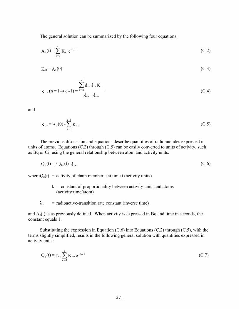
271

The general solution can be summarized by the following four equations:

and

The previous discussion and equations describe quantities of radionuclides expressed in units of atoms. Equations (C.2) through (C.5) can be easily converted to units of activity, such as Bq or Ci, using the general relationship between atom and activity units:

where Qc(t) = activity of chain member c at time t (activity units) k = constant of proportionality between activity units and atoms

(activity·time/atom) rc = radioactive-transition rate constant (inverse time) and Ac(t) is as previously defined. When activity is expressed in Bq and time in seconds, the constant equals 1. Substituting the expression in Equation (C.6) into Equations (C.2) through (C.5), with the terms slightly simplified, results in the following general solution with quantities expressed in activity units:

e K = (t)A t -i c

c

1 = ic

ei (C.2)

(0)A = K 11 1 (C.3)

n ec e

n iir c i

1 - c

n = in c

-

K d = 1) - c 1 =(n K

(C.4)

K - (0)A = K n c

1 - c

1 =n cc c (C.5)

cr cc (t)Ak = (t)Q (C.6)

e K = (t)Q t -n c

c

1 =n cr c

n e (C.7)

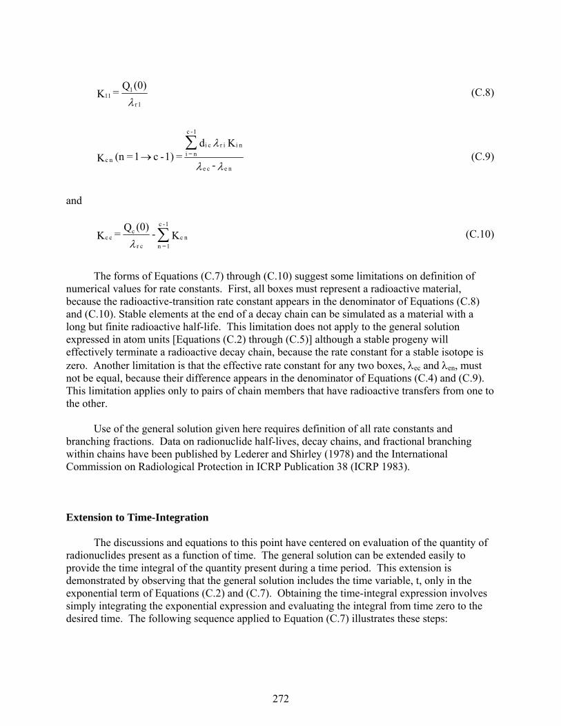
272

and

The forms of Equations (C.7) through (C.10) suggest some limitations on definition of numerical values for rate constants. First, all boxes must represent a radioactive material, because the radioactive-transition rate constant appears in the denominator of Equations (C.8) and (C.10). Stable elements at the end of a decay chain can be simulated as a material with a long but finite radioactive half-life. This limitation does not apply to the general solution expressed in atom units [Equations (C.2) through (C.5)] although a stable progeny will effectively terminate a radioactive decay chain, because the rate constant for a stable isotope is zero. Another limitation is that the effective rate constant for any two boxes, ec and en, must not be equal, because their difference appears in the denominator of Equations (C.4) and (C.9). This limitation applies only to pairs of chain members that have radioactive transfers from one to the other. Use of the general solution given here requires definition of all rate constants and branching fractions. Data on radionuclide half-lives, decay chains, and fractional branching within chains have been published by Lederer and Shirley (1978) and the International Commission on Radiological Protection in ICRP Publication 38 (ICRP 1983). Extension to Time-Integration The discussions and equations to this point have centered on evaluation of the quantity of radionuclides present as a function of time. The general solution can be extended easily to provide the time integral of the quantity present during a time period. This extension is demonstrated by observing that the general solution includes the time variable, t, only in the exponential term of Equations (C.2) and (C.7). Obtaining the time-integral expression involves simply integrating the exponential expression and evaluating the integral from time zero to the desired time. The following sequence applied to Equation (C.7) illustrates these steps:

1r

11 1

(0)Q = K (C.8)

n ec e

n iir c i

1 - c

n = in c

-

K d = 1) - c 1 =(n K

(C.9)

K - (0)Q

= K n c

1 - c

1 =n cr

cc c

(C.10)

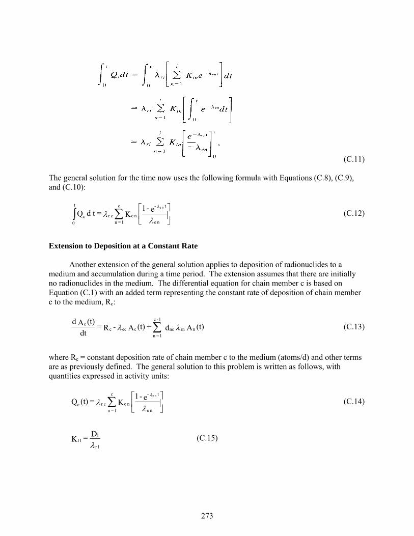
273

The general solution for the time now uses the following formula with Equations (C.8), (C.9), and (C.10):

Extension to Deposition at a Constant Rate Another extension of the general solution applies to deposition of radionuclides to a medium and accumulation during a time period. The extension assumes that there are initially no radionuclides in the medium. The differential equation for chain member c is based on Equation (C.1) with an added term representing the constant rate of deposition of chain member c to the medium, Rc:

where Rc = constant deposition rate of chain member c to the medium (atoms/d) and other terms are as previously defined. The general solution to this problem is written as follows, with quantities expressed in activity units:

(C.11)

n e

t -

n c

c

1 =n cr c

t

0

e - 1 K = t d Q

n e

(C.12)

(t)A d + (t)A - R = dt

(t)A dnrnnc

1 - c

1 =n cecc

c (C.13)

n e

t -

n c

c

1 =n cr c

e - 1 K = (t)Qn e

(C.14)

1r

11 1

D = K (C.15)

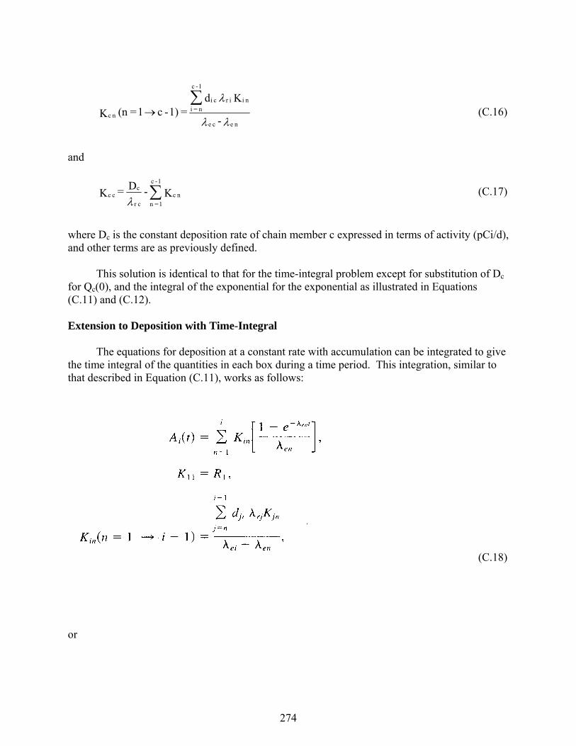
274

and

where Dc is the constant deposition rate of chain member c expressed in terms of activity (pCi/d), and other terms are as previously defined. This solution is identical to that for the time-integral problem except for substitution of Dc for Qc(0), and the integral of the exponential for the exponential as illustrated in Equations (C.11) and (C.12). Extension to Deposition with Time-Integral The equations for deposition at a constant rate with accumulation can be integrated to give the time integral of the quantities in each box during a time period. This integration, similar to that described in Equation (C.11), works as follows:

or

n ec e

n iir c i

1 - c

n = in c

-

K d = 1) - c 1 =(n K

(C.16)

K - D = K n c

1 - c

1 =n cr

cc c

(C.17)

(C.18)

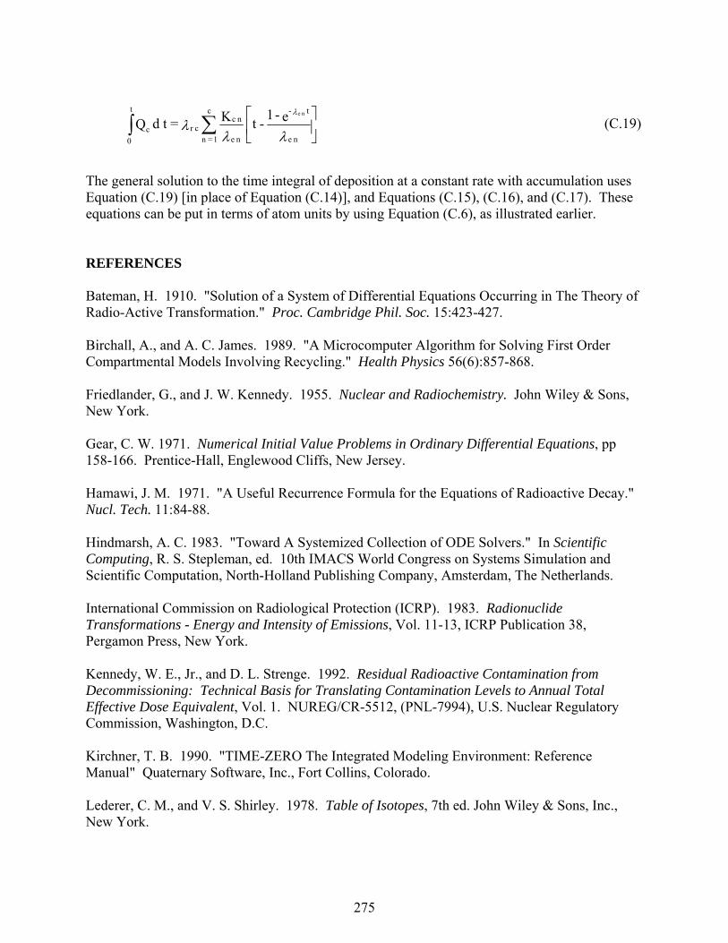
275

The general solution to the time integral of deposition at a constant rate with accumulation uses Equation (C.19) [in place of Equation (C.14)], and Equations (C.15), (C.16), and (C.17). These equations can be put in terms of atom units by using Equation (C.6), as illustrated earlier. REFERENCES Bateman, H. 1910. "Solution of a System of Differential Equations Occurring in The Theory of Radio-Active Transformation." Proc. Cambridge Phil. Soc. 15:423-427. Birchall, A., and A. C. James. 1989. "A Microcomputer Algorithm for Solving First Order Compartmental Models Involving Recycling." Health Physics 56(6):857-868. Friedlander, G., and J. W. Kennedy. 1955. Nuclear and Radiochemistry. John Wiley & Sons, New York. Gear, C. W. 1971. Numerical Initial Value Problems in Ordinary Differential Equations, pp 158-166. Prentice-Hall, Englewood Cliffs, New Jersey. Hamawi, J. M. 1971. "A Useful Recurrence Formula for the Equations of Radioactive Decay." Nucl. Tech. 11:84-88. Hindmarsh, A. C. 1983. "Toward A Systemized Collection of ODE Solvers." In Scientific Computing, R. S. Stepleman, ed. 10th IMACS World Congress on Systems Simulation and Scientific Computation, North-Holland Publishing Company, Amsterdam, The Netherlands. International Commission on Radiological Protection (ICRP). 1983. Radionuclide Transformations - Energy and Intensity of Emissions, Vol. 11-13, ICRP Publication 38, Pergamon Press, New York. Kennedy, W. E., Jr., and D. L. Strenge. 1992. Residual Radioactive Contamination from Decommissioning: Technical Basis for Translating Contamination Levels to Annual Total Effective Dose Equivalent, Vol. 1. NUREG/CR-5512, (PNL-7994), U.S. Nuclear Regulatory Commission, Washington, D.C. Kirchner, T. B. 1990. "TIME-ZERO The Integrated Modeling Environment: Reference Manual" Quaternary Software, Inc., Fort Collins, Colorado. Lederer, C. M., and V. S. Shirley. 1978. Table of Isotopes, 7th ed. John Wiley & Sons, Inc., New York.

n e

t -

n e

n cc

1 =n cr c

t

0

e - 1 -t K = t d Q

n e

(C.19)

276

Scherpelz, R. Il, and A. E. Desrosiers. 1980. "A Modification to a Recurrence Formula for Linear First-Order Equations." Health Physics 40:905-907. Skrable, K., C. French., G. Chabot, and A. Hajor. 1974. "A General Equation for the Kinetics of Linear First Order Phenomena and Suggested Applications." Health Physics 27:155-57.

277

APPENDIX D

278

APPENDIX D: TRANSFER FACTORS The transfer factor, also known as the concentration ratio or bioaccumulation factor, is the ratio of the concentration of an element in an organism of interest to the concentration in the source medium. The transfer factor applies to long-term, chronic exposure of plants and animals and is ideally measured at equilibrium. Transfer factors relate the concentration of an element in soil to the element’s concentration in plant products and the concentration in animal feed to animal products; the fish transfer factor relates the concentration in water to the concentration in fish muscle tissue. Transfer factors are used in risk assessments to estimate the amount of radioactivity that could be present in a food crop or organism based on the calculated concentration in the source medium (i.e., soil or animal feed). By calculating the concentration in the food, the total intake can be estimated and a dose calculated as a result of the annual intake. In terms of radionuclides, the transfer factor is used to calculate how many curies per kilogram of soil are transferred to the edible dry plant product (Bq per kg). For vegetation, the units are kg soil/kg edible dry plants. For animal products, the transfer factor relates the daily intake to that of the animal product. Units for milk are Bq/L per Bq intake/d. For animal and fish meat products, transfer factors are measured in wet weight animal product: Bq/kg muscle per Bq/d intake for meat and Bq/kg muscle per Bq/L for fish. Numerous studies have been undertaken to quantify transfer factors for specific chemical elements as a function of food type. These studies have been compiled in several publications. This document was written to compile a list of those transfer factors which best describe the commonly accepted factors, and to document the data sources by providing the original as well as the compilation references. In some cases, this listing contains values for elements that are not included in other compilations. Transfer factors for such elements were extrapolated from experimental data based on chemical similarities. D.1 Selection of Transfer Factors Transfer factors for this listing were generally selected from recommended values compiled by national or international organizations for use in radiological food chain transport calculations. (In some cases, where newer data were available, very recent references for specific values were preferred to compiled recommendations.) In general, the recommended values from more recent compilations were selected rather than those in older publications. The primary data sources are also cited where identified in the compilation document. In many cases, where neither a primary source of data nor a recommended value in a compilation was available, other methods were used to estimate transfer factors, as described in the following sections. D.2 Compilations of Data Sources A hierarchy of data sources was established to select recommended values for transfer factors. The most recent and comprehensive references were given priority. The first reference chosen was the International Atomic Energy Agency’s Technical Report Series #364, Handbook of Parameter Values for the Prediction of Radionuclide Transfer in Temperate Environments (IAEA 1994). This document encompasses a wide variety of plant types and is the result of

279

extensive background investigations. It is based on data compiled by the International Union of Radioecologists. The second reference given consideration was the NUREG/CR-5512, Residual Radioactive Contamination From Decommissioning: Technical Basis for Translating Contamination Levels to Annual Total Effective Dose Equivalent (Kennedy and Strenge 1992) because of its large set of data and traceable references. Other references used to fill in data were the NCRP Report #123 (1996), Screening Models for Releases of Radionuclides to Atmosphere, Surface Water, and Ground, the library from the GENII Version 1.485 system of computer codes (Napier et al. 1988), and the series of documents by Coughtrey et al., Radionuclide Distribution and Transport in Terrestrial and Aquatic Ecosystems, Vols. 1-6 (1983). The NCRP Report #123 was chosen because it is a generally accepted reference for a generic model. The GENII V.1.485 values have been in use for a decade to model the semi-arid environment at Hanford and are reasonably well documented. Although the methodology for the Coughtrey and Thorne values was somewhat different, resulting in high values for transfer factors, it was necessary to use their values to fill in data where no other information was available. When no referenceable documents were available, data were derived based on chemical groupings in the periodic table of the elements, as described below. D.3 Food Types Evaluated For this compendium of data, foods were grouped into the following types: meat, milk, poultry, eggs, fish, leafy vegetables, other (root) vegetables, fruit, and grain. When more than one food was listed for a given food type (e.g., spinach, cabbage and lettuce listed as leafy vegetable), the transfer factor for each food was weighted by the U.S. Department of Agriculture annual per capita consumption rate (USDA 1983), and a weighted average of transfer factors was reported for that food type. Plant transfer factors from the IAEA Handbook #364, NUREG/CR-5512, GENII, and Coughtrey et al. are based on dry weight data (Bq per kg dry crop edible product)/(Bq/kg dry soil in the upper 20 cm). When data were presented on a wet weight basis, they were converted to dry weight using conversion factors found in Table D.1. All plant transfer factors presented in this report are based on dry weight. Animal products are presented on a wet weight or volume (milk) basis. D.4 Methods Used to Estimate Transfer Factors Experimental data are not available for all elements for all food types. Therefore, several methods were employed to estimate transfer factors for elements and food types where experimental data were lacking. In some cases, parameters from one vegetable type were applied to remaining vegetable types for the same element. In these cases, no adjustments were made for the wet/dry ratios for specific food types, due to the relatively large uncertainty inherent in applying the transfer factor from one food type to another. In other cases, chemical similarities among elements were the basis for estimating the transfer factor. If two or more transfer factors were available for elements in a chemical group, the geometric mean was calculated from the chemical group for the given food type (Figure 1). Where data were avail-able for only one element in a chemical group, the transfer factor for that element was applied to other elements in the same chemical group. Specific cases are listed in the Estimated Transfer

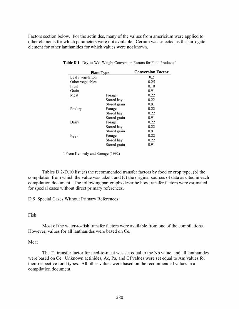
280

Factors section below. For the actinides, many of the values from americium were applied to other elements for which parameters were not available. Cerium was selected as the surrogate element for other lanthanides for which values were not known.

Table D.1. Dry-to-Wet-Weight Conversion Factors for Food Products a

Plant Type Conversion Factor Leafy vegetation 0.2 Other vegetables 0.25 Fruit 0.18 Grain 0.91 Meat Forage 0.22 Stored hay 0.22 Stored grain 0.91 Poultry Forage 0.22 Stored hay 0.22 Stored grain 0.91 Dairy Forage 0.22 Stored hay 0.22 Stored grain 0.91 Eggs Forage 0.22 Stored hay 0.22 Stored grain 0.91

a From Kennedy and Strenge (1992) Tables D.2-D.10 list (a) the recommended transfer factors by food or crop type, (b) the compilation from which the value was taken, and (c) the original sources of data as cited in each compilation document. The following paragraphs describe how transfer factors were estimated for special cases without direct primary references. D.5 Special Cases Without Primary References Fish Most of the water-to-fish transfer factors were available from one of the compilations. However, values for all lanthanides were based on Ce. Meat The Ta transfer factor for feed-to-meat was set equal to the Nb value, and all lanthanides were based on Ce. Unknown actinides, Ac, Pa, and Cf values were set equal to Am values for their respective food types. All other values were based on the recommended values in a compilation document.

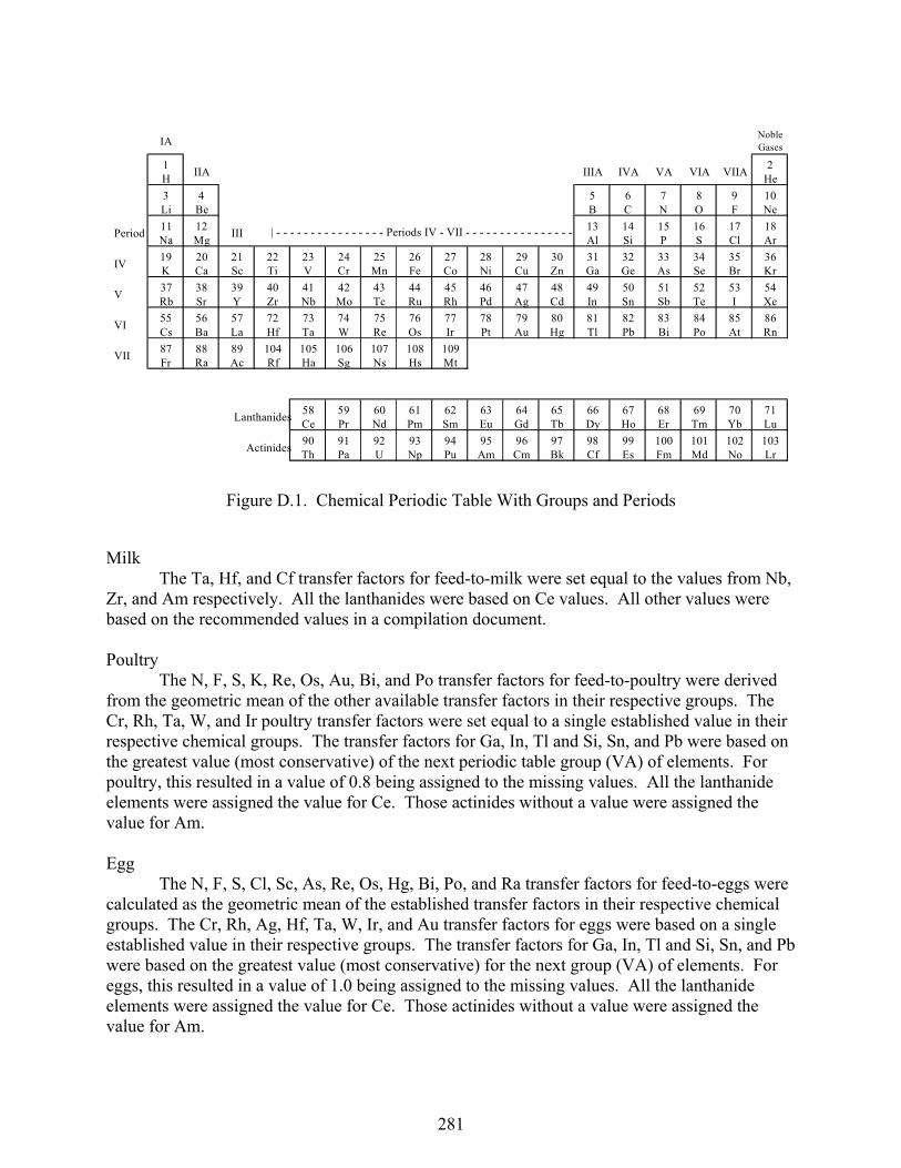
281

IANobleGases

1H

IIA IIIA IVA VA VIA VIIA2

He

3Li

4Be

5B

6C

7N

8O

9F

10Ne

Period11Na

12Mg

III13Al

14Si

15P

16S

17Cl

18Ar

IV19K

20Ca

21Sc

22Ti

23V

24Cr

25Mn

26Fe

27Co

28Ni

29Cu

30Zn

31Ga

32Ge

33As

34Se

35Br

36Kr

V37Rb

38Sr

39Y

40Zr

41Nb

42Mo

43Tc

44Ru

45Rh

46Pd

47Ag

48Cd

49In

50Sn

51Sb

52Te

53I

54Xe

VI55Cs

56Ba

57La

72Hf

73Ta

74W

75Re

76Os

77Ir

78Pt

79Au

80Hg

81Tl

82Pb

83Bi

84Po

85At

86Rn

VII87Fr

88Ra

89Ac

104Rf

105Ha

106Sg

107Ns

108Hs

109Mt

Lanthanides58Ce

59Pr

60Nd

61Pm

62Sm

63Eu

64Gd

65Tb

66Dy

67Ho

68Er

69Tm

70Yb

71Lu

Actinides90Th

91Pa

92U

93Np

94Pu

95Am

96Cm

97Bk

98Cf

99Es

100Fm

101Md

102No

103Lr

| - - - - - - - - - - - - - - - - Periods IV - VII - - - - - - - - - - - - - - - -

Figure D.1. Chemical Periodic Table With Groups and Periods

Milk The Ta, Hf, and Cf transfer factors for feed-to-milk were set equal to the values from Nb, Zr, and Am respectively. All the lanthanides were based on Ce values. All other values were based on the recommended values in a compilation document. Poultry The N, F, S, K, Re, Os, Au, Bi, and Po transfer factors for feed-to-poultry were derived from the geometric mean of the other available transfer factors in their respective groups. The Cr, Rh, Ta, W, and Ir poultry transfer factors were set equal to a single established value in their respective chemical groups. The transfer factors for Ga, In, Tl and Si, Sn, and Pb were based on the greatest value (most conservative) of the next periodic table group (VA) of elements. For poultry, this resulted in a value of 0.8 being assigned to the missing values. All the lanthanide elements were assigned the value for Ce. Those actinides without a value were assigned the value for Am. Egg The N, F, S, Cl, Sc, As, Re, Os, Hg, Bi, Po, and Ra transfer factors for feed-to-eggs were calculated as the geometric mean of the established transfer factors in their respective chemical groups. The Cr, Rh, Ag, Hf, Ta, W, Ir, and Au transfer factors for eggs were based on a single established value in their respective groups. The transfer factors for Ga, In, Tl and Si, Sn, and Pb were based on the greatest value (most conservative) for the next group (VA) of elements. For eggs, this resulted in a value of 1.0 being assigned to the missing values. All the lanthanide elements were assigned the value for Ce. Those actinides without a value were assigned the value for Am.

282

Fruit The soil-to-fruit transfer factors for N, Os, Au, and Hg were calculated based on the geometric mean of the transfer factors in their respective groups on the periodic table. Hafnium (Hf) and Ta were assigned values equal to those for Zr and Nb, respectively. All the lanthanide elements were assigned the value for Ce. Grain The soil-to-grain transfer factors for Be, N, and Hg were calculated as the geometric mean of the transfer factors in their respective periodic table groups. Silver (Ag), Hf, Ta, and Au transfer factors for grain were based on the single known value in their respective chemical groups. All the lanthanide elements were assigned the value for Ce. The grain transfer factors for Ac, Pa, and Cf were based on Am. Leafy Vegetation The soil-to-leafy vegetation transfer factors for N, Hf, Ta, and Au were calculated as the geometric means of the transfer factors in their respective periodic table groups. All the lanthanide elements were assigned the value for Ce. Actinium (Ac), Pa, and Cf were assigned the leafy vegetable transfer factor from Am. Root Vegetables The soil-to-root transfer factors for N and Au were calculated as the geometric mean of the transfer factors in their respective periodic table groups. Hafnium (Hf) and Ta were based on a single established value in their respective chemical groups. The root transfer factors for Ac, Pa, and Cf were based on Am. All lanthanide elements were assigned the value for Ce. D.6 Additional Transfer Factors used in GENII-V2 Three additional types of transfer factors are used in GENII-V2; these are all derived from the earlier GENII 1.485 (Napier et al. 1988) without current updating. These are the transfer factors for saltwater fish, fresh and salt water crustaceans, fresh and salt water molluscs, and fresh and salt water plants. These are listed in Tables D.11, D.12, D.13, and D.14. All transfer factors in these tables come from the GENII 1.485 data files. For marine species, the GENII 1.485 values in Napier et al. (1988) are largely traceable back to A Model for the Approximate Calculation of Safe Rates of Discharge of Radioactive Wastes into Marine Environments (Freke 1967). Specifically for freshwater environments, the parameters are ultimately traceable to Concentration Factors of Chemical Elements in Edible Aquatic Organisms (Thompson et al. 1972), which in turn is primarily derived from Ng’s (1968) Handbook for Estimating the Maximum Internal Dose from Radionuclides Released to the Biosphere.

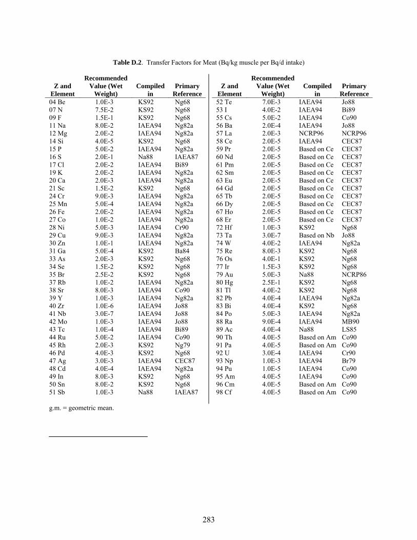
283

Table D.2. Transfer Factors for Meat (Bq/kg muscle per Bq/d intake)

Z and Element

Recommended Value (Wet

Weight) Compiled

in Primary

Reference 04 Be 1.0E-3 KS92 Ng68 07 N 7.5E-2 KS92 Ng68 09 F 1.5E-1 KS92 Ng68 11 Na 8.0E-2 IAEA94 Ng82a 12 Mg 2.0E-2 IAEA94 Ng82a 14 Si 4.0E-5 KS92 Ng68 15 P 5.0E-2 IAEA94 Ng82a 16 S 2.0E-1 Na88 IAEA87 17 Cl 2.0E-2 IAEA94 Bi89 19 K 2.0E-2 IAEA94 Ng82a 20 Ca 2.0E-3 IAEA94 Ng82a 21 Sc 1.5E-2 KS92 Ng68 24 Cr 9.0E-3 IAEA94 Ng82a 25 Mn 5.0E-4 IAEA94 Ng82a 26 Fe 2.0E-2 IAEA94 Ng82a 27 Co 1.0E-2 IAEA94 Ng82a 28 Ni 5.0E-3 IAEA94 Cr90 29 Cu 9.0E-3 IAEA94 Ng82a 30 Zn 1.0E-1 IAEA94 Ng82a 31 Ga 5.0E-4 KS92 Ba84 33 As 2.0E-3 KS92 Ng68 34 Se 1.5E-2 KS92 Ng68 35 Br 2.5E-2 KS92 Ng68 37 Rb 1.0E-2 IAEA94 Ng82a 38 Sr 8.0E-3 IAEA94 Co90 39 Y 1.0E-3 IAEA94 Ng82a 40 Zr 1.0E-6 IAEA94 Jo88 41 Nb 3.0E-7 IAEA94 Jo88 42 Mo 1.0E-3 IAEA94 Jo88 43 Tc 1.0E-4 IAEA94 Bi89 44 Ru 5.0E-2 IAEA94 Co90 45 Rh 2.0E-3 KS92 Ng79 46 Pd 4.0E-3 KS92 Ng68 47 Ag 3.0E-3 IAEA94 CEC87 48 Cd 4.0E-4 IAEA94 Ng82a 49 In 8.0E-3 KS92 Ng68 50 Sn 8.0E-2 KS92 Ng68 51 Sb 1.0E-3 Na88 IAEA87

Z and Element

Recommended Value (Wet

Weight) Compiled

in Primary

Reference 52 Te 7.0E-3 IAEA94 Jo88 53 I 4.0E-2 IAEA94 Bi89 55 Cs 5.0E-2 IAEA94 Co90 56 Ba 2.0E-4 IAEA94 Jo88 57 La 2.0E-3 NCRP96 NCRP96 58 Ce 2.0E-5 IAEA94 CEC87 59 Pr 2.0E-5 Based on Ce CEC87 60 Nd 2.0E-5 Based on Ce CEC87 61 Pm 2.0E-5 Based on Ce CEC87 62 Sm 2.0E-5 Based on Ce CEC87 63 Eu 2.0E-5 Based on Ce CEC87 64 Gd 2.0E-5 Based on Ce CEC87 65 Tb 2.0E-5 Based on Ce CEC87 66 Dy 2.0E-5 Based on Ce CEC87 67 Ho 2.0E-5 Based on Ce CEC87 68 Er 2.0E-5 Based on Ce CEC87 72 Hf 1.0E-3 KS92 Ng68 73 Ta 3.0E-7 Based on Nb Jo88 74 W 4.0E-2 IAEA94 Ng82a 75 Re 8.0E-3 KS92 Ng68 76 Os 4.0E-1 KS92 Ng68 77 Ir 1.5E-3 KS92 Ng68 79 Au 5.0E-3 Na88 NCRP86 80 Hg 2.5E-1 KS92 Ng68 81 Tl 4.0E-2 KS92 Ng68 82 Pb 4.0E-4 IAEA94 Ng82a 83 Bi 4.0E-4 KS92 Ng68 84 Po 5.0E-3 IAEA94 Ng82a 88 Ra 9.0E-4 IAEA94 MB90 89 Ac 4.0E-4 Na88 LS85 90 Th 4.0E-5 Based on Am Co90 91 Pa 4.0E-5 Based on Am Co90 92 U 3.0E-4 IAEA94 Cr90 93 Np 1.0E-3 IAEA94 Br79 94 Pu 1.0E-5 IAEA94 Co90 95 Am 4.0E-5 IAEA94 Co90 96 Cm 4.0E-5 Based on Am Co90 98 Cf 4.0E-5 Based on Am Co90

g.m. = geometric mean.

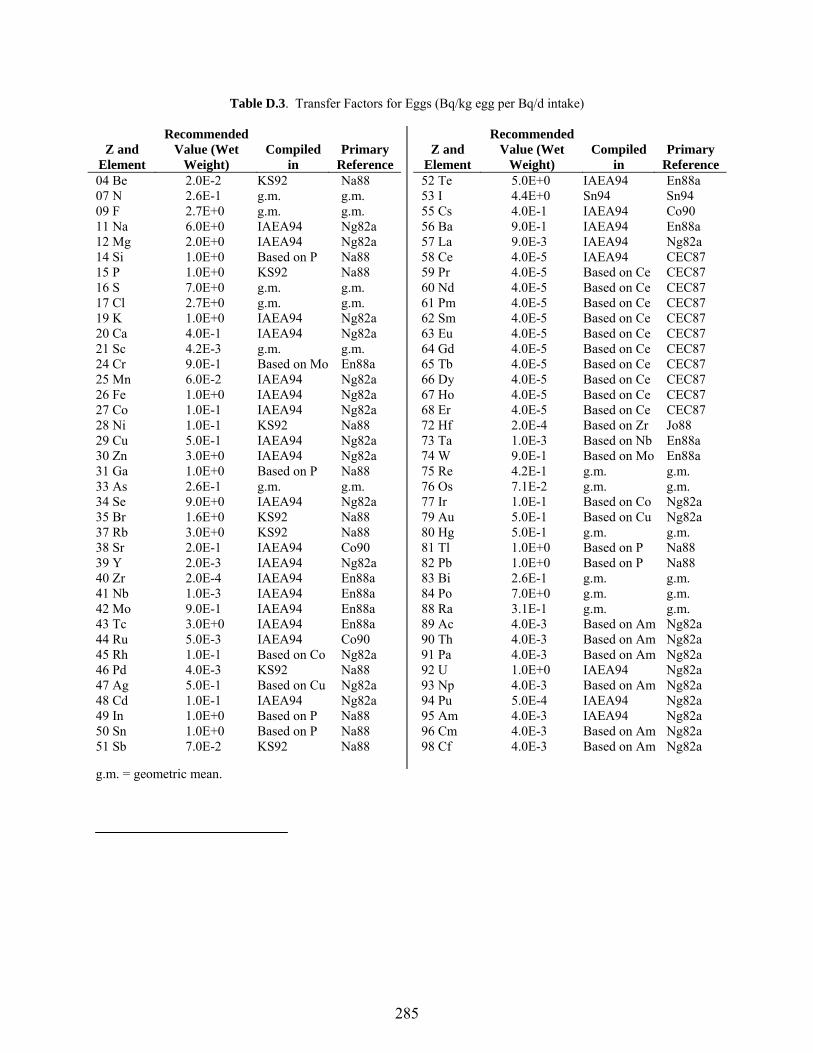
285

Table D.3. Transfer Factors for Eggs (Bq/kg egg per Bq/d intake)

Z and Element

Recommended Value (Wet

Weight) Compiled

in Primary

Reference 04 Be 2.0E-2 KS92 Na88 07 N 2.6E-1 g.m. g.m. 09 F 2.7E+0 g.m. g.m. 11 Na 6.0E+0 IAEA94 Ng82a 12 Mg 2.0E+0 IAEA94 Ng82a 14 Si 1.0E+0 Based on P Na88 15 P 1.0E+0 KS92 Na88 16 S 7.0E+0 g.m. g.m. 17 Cl 2.7E+0 g.m. g.m. 19 K 1.0E+0 IAEA94 Ng82a 20 Ca 4.0E-1 IAEA94 Ng82a 21 Sc 4.2E-3 g.m. g.m. 24 Cr 9.0E-1 Based on Mo En88a 25 Mn 6.0E-2 IAEA94 Ng82a 26 Fe 1.0E+0 IAEA94 Ng82a 27 Co 1.0E-1 IAEA94 Ng82a 28 Ni 1.0E-1 KS92 Na88 29 Cu 5.0E-1 IAEA94 Ng82a 30 Zn 3.0E+0 IAEA94 Ng82a 31 Ga 1.0E+0 Based on P Na88 33 As 2.6E-1 g.m. g.m. 34 Se 9.0E+0 IAEA94 Ng82a 35 Br 1.6E+0 KS92 Na88 37 Rb 3.0E+0 KS92 Na88 38 Sr 2.0E-1 IAEA94 Co90 39 Y 2.0E-3 IAEA94 Ng82a 40 Zr 2.0E-4 IAEA94 En88a 41 Nb 1.0E-3 IAEA94 En88a 42 Mo 9.0E-1 IAEA94 En88a 43 Tc 3.0E+0 IAEA94 En88a 44 Ru 5.0E-3 IAEA94 Co90 45 Rh 1.0E-1 Based on Co Ng82a 46 Pd 4.0E-3 KS92 Na88 47 Ag 5.0E-1 Based on Cu Ng82a 48 Cd 1.0E-1 IAEA94 Ng82a 49 In 1.0E+0 Based on P Na88 50 Sn 1.0E+0 Based on P Na88 51 Sb 7.0E-2 KS92 Na88

Z and Element

Recommended Value (Wet

Weight) Compiled

in Primary

Reference 52 Te 5.0E+0 IAEA94 En88a 53 I 4.4E+0 Sn94 Sn94 55 Cs 4.0E-1 IAEA94 Co90 56 Ba 9.0E-1 IAEA94 En88a 57 La 9.0E-3 IAEA94 Ng82a 58 Ce 4.0E-5 IAEA94 CEC87 59 Pr 4.0E-5 Based on Ce CEC87 60 Nd 4.0E-5 Based on Ce CEC87 61 Pm 4.0E-5 Based on Ce CEC87 62 Sm 4.0E-5 Based on Ce CEC87 63 Eu 4.0E-5 Based on Ce CEC87 64 Gd 4.0E-5 Based on Ce CEC87 65 Tb 4.0E-5 Based on Ce CEC87 66 Dy 4.0E-5 Based on Ce CEC87 67 Ho 4.0E-5 Based on Ce CEC87 68 Er 4.0E-5 Based on Ce CEC87 72 Hf 2.0E-4 Based on Zr Jo88 73 Ta 1.0E-3 Based on Nb En88a 74 W 9.0E-1 Based on Mo En88a 75 Re 4.2E-1 g.m. g.m. 76 Os 7.1E-2 g.m. g.m. 77 Ir 1.0E-1 Based on Co Ng82a 79 Au 5.0E-1 Based on Cu Ng82a 80 Hg 5.0E-1 g.m. g.m. 81 Tl 1.0E+0 Based on P Na88 82 Pb 1.0E+0 Based on P Na88 83 Bi 2.6E-1 g.m. g.m. 84 Po 7.0E+0 g.m. g.m. 88 Ra 3.1E-1 g.m. g.m. 89 Ac 4.0E-3 Based on Am Ng82a 90 Th 4.0E-3 Based on Am Ng82a 91 Pa 4.0E-3 Based on Am Ng82a 92 U 1.0E+0 IAEA94 Ng82a 93 Np 4.0E-3 Based on Am Ng82a 94 Pu 5.0E-4 IAEA94 Ng82a 95 Am 4.0E-3 IAEA94 Ng82a 96 Cm 4.0E-3 Based on Am Ng82a 98 Cf 4.0E-3 Based on Am Ng82a

g.m. = geometric mean.

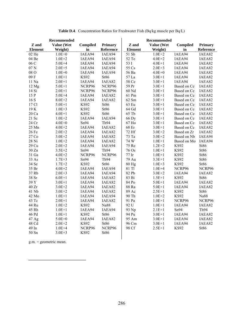
286

Table D.4. Concentration Ratios for Freshwater Fish (Bq/kg muscle per Bq/L)

Z and Element

Recommended Value (Wet

Weight) Compiled

in Primary

Reference 02 He 1.0E+0 IAEA94 IAEA94 04 Be 1.0E+2 IAEA94 IAEA94 06 C 5.0E+4 IAEA94 IAEA94 07 N 2.0E+5 IAEA94 IAEA94 08 O 1.0E+0 IAEA94 IAEA94 09 F 1.0E+1 KS92 St86 11 Na 2.0E+1 IAEA94 IAEA82 12 Mg 5.0E+1 NCRP96 NCRP96 14 Si 2.0E+1 NCRP96 NCRP96 15 P 5.0E+4 IAEA94 IAEA82 16 S 8.0E+2 IAEA94 IAEA82 17 Cl 5.0E+1 KS92 St86 19 K 1.0E+3 KS92 St86 20 Ca 4.0E+1 KS92 St86 21 Sc 1.0E+2 IAEA94 IAEA94 24 Cr 4.0E+0 Sn94 Th94 25 Mn 4.0E+2 IAEA94 IAEA82 26 Fe 2.0E+2 IAEA94 IAEA82 27 Co 3.0E+2 IAEA94 IAEA82 28 Ni 1.0E+2 IAEA94 IAEA82 29 Cu 2.0E+2 IAEA94 IAEA94 30 Zn 3.5E+2 Sn94 Th94 31 Ga 4.0E+2 NCRP96 NCRP96 33 As 1.7E+3 Sn94 Th94 34 Se 1.7E+2 KS92 St86 35 Br 4.0E+2 IAEA94 IAEA94 37 Rb 2.0E+3 IAEA94 IAEA94 38 Sr 6.0E+1 IAEA94 IAEA82 39 Y 3.0E+1 IAEA94 IAEA82 40 Zr 3.0E+2 IAEA94 IAEA82 41 Nb 3.0E+2 IAEA94 IAEA82 42 Mo 1.0E+1 IAEA94 IAEA94 43 Tc 2.0E+1 IAEA94 IAEA82 44 Ru 1.0E+2 KS92 Na88 45 Rh 1.0E+1 IAEA94 IAEA94 46 Pd 1.0E+1 KS92 St86 47 Ag 5.0E+0 IAEA94 IAEA82 48 Cd 2.0E+2 KS92 St86 49 In 1.0E+4 NCRP96 NCRP96 50 Sn 3.0E+3 KS92 St86

Z and Element

Recommended Value (Wet

Weight) Compiled

in Primary

Reference 51 Sb 1.0E+2 IAEA94 IAEA82 52 Te 4.0E+2 IAEA94 IAEA82 53 I 4.0E+1 IAEA94 IAEA82 55 Cs 2.0E+3 IAEA94 IAEA82 56 Ba 4.0E+0 IAEA94 IAEA82 57 La 3.0E+1 IAEA94 IAEA82 58 Ce 3.0E+1 IAEA94 IAEA82 59 Pr 3.0E+1 Based on Ce IAEA82 60 Nd 3.0E+1 Based on Ce IAEA82 61 Pm 3.0E+1 Based on Ce IAEA82 62 Sm 3.0E+1 Based on Ce IAEA82 63 Eu 3.0E+1 Based on Ce IAEA82 64 Gd 3.0E+1 Based on Ce IAEA82 65 Tb 3.0E+1 Based on Ce IAEA82 66 Dy 3.0E+1 Based on Ce IAEA82 67 Ho 3.0E+1 Based on Ce IAEA82 68 Er 3.0E+1 Based on Ce IAEA82 72 Hf 3.0E+2 Based on Zr IAEA82 73 Ta 3.0E+2 Based on Nb IAEA94 74 W 1.0E+1 Based on Mo IAEA94 75 Re 1.2E+2 KS92 St86 76 Os 1.0E+1 KS92 St86 77 Ir 1.0E+1 KS92 St86 79 Au 3.3E+1 KS92 St86 80 Hg 1.0E+3 KS92 St86 81 Tl 1.0E+4 NCRP96 NCRP96 82 Pb 3.0E+2 IAEA94 IAEA82 83 Bi 1.5E+1 KS92 St86 84 Po 5.0E+1 IAEA94 IAEA82 88 Ra 5.0E+1 IAEA94 IAEA82 89 Ac 2.5E+1 KS92 St86 90 Th 1.0E+2 KS92 Na88 91 Pa 1.0E+1 NCRP96 NCRP96 92 U 1.0E+1 IAEA94 IAEA82 93 Np 2.1E+1 Sn94 Th94 94 Pu 3.0E+1 IAEA94 IAEA82 95 Am 3.0E+1 IAEA94 IAEA82 96 Cm 3.0E+1 IAEA94 IAEA82 98 Cf 2.5E+1 KS92 St86

g.m. = geometric mean.

287

Table D.5. Transfer Factors for Fruit (Bq/kg fruit per Bq/kg soil)

Z and Element

Recommended Value (Dry

Weight) Compiled

in Primary

Reference 04 Be 1.5E-3 KS92 Ba84 06 C 7.0E-1 Na88 Na88 07 N 3.0E-2 g.m. g.m. 09 F 6.0E-3 KS92 Ba84 11 Na 3.0E-1 IAEA94 Ng82b 12 Mg 5.5E-1 KS92 Ba84 14 Si 7.0E-2 KS92 Ba84 15 P 3.5E+0 KS92 Ba84 16 S 1.5E+0 KS92 Ba84 17 Cl 7.0E+1 KS92 Ba84 19 K 5.5E-1 KS92 Ba84 20 Ca 3.5E-1 KS92 Ba84 21 Sc 1.0E-3 KS92 Ba84 24 Cr 4.5E-3 KS92 Ba84 25 Mn 5.0E-2 KS92 Ba84 26 Fe 5.0E-2 CT83 CT83 27 Co 7.0E-3 KS92 Ba84 28 Ni 6.0E-2 KS92 Ba84 29 Cu 2.5E-1 KS92 Ba84 30 Zn 9.0E-1 KS92 Ba84 31 Ga 4.0E-4 Based on In Ba84 33 As 6.0E-3 KS92 Ba84 34 Se 5.0E-2 CT83 CT83 35 Br 1.5E+0 KS92 Fu78 37 Rb 9.0E-1 IAEA94 Ng82b 38 Sr 2.0E-1 IAEA94 Fr82 39 Y 1.0E-2 IAEA94 Ng82b 40 Zr 1.0E-3 IAEA94 Ng82b 41 Nb 2.5E-2 CT83 CT83 42 Mo 5.0E-2 CT83 CT83 43 Tc 1.5E+0 KS92 Ba84 44 Ru 4.0E-2 IAEA94 Ng82b 45 Rh 4.0E-2 KS92 Ba84 46 Pd 4.0E-2 KS92 Ba84 47 Ag 8.0E-4 IAEA94 Fr89 48 Cd 1.5E-1 KS92 Ba84 49 In 4.0E-4 KS92 Fu78 50 Sn 6.0E-3 KS92 Fu78 51 Sb 8.0E-5 KS92 IUR89

Z and Element

Recommended Value (Dry

Weight) Compiled

in Primary

Reference 52 Te 4.0E-3 KS92 Ba84 53 I 4.0E-2 Sn94 Sn94 55 Cs 2.2E-1 IAEA94 Fr89 56 Ba 1.5E-2 KS92 Ba84 57 La 4.0E-3 KS92 Ba84 58 Ce 2.0E-2 Ng82b Ng82b 59 Pr 2.0E-2 Based on Ce Ng82b 60 Nd 2.0E-2 Based on Ce Ng82b 61 Pm 2.0E-2 Based on Ce Ng82b 62 Sm 2.0E-2 Based on Ce Ng82b 63 Eu 2.0E-2 Based on Ce Ng82b 64 Gd 2.0E-2 Based on Ce Ng82b 65 Tb 2.0E-2 Based on Ce Ng82b 66 Dy 2.0E-2 Based on Ce Ng82b 67 Ho 2.0E-2 Based on Ce Ng82b 68 Er 2.0E-2 Based on Ce Ng82b 72 Hf 1.0E-3 Based on Zr Ng82b 73 Ta 2.5E-2 Based on Nb CT83 74 W 3.0E+0 NCRP96 NCRP96 75 Re 3.5E-1 KS92 Ba84 76 Os 4.5E-2 g.m. g.m. 77 Ir 1.5E-2 KS92 Ba84 79 Au 1.4E-2 g.m. g.m. 80 Hg 3.7E-1 g.m. g.m. 81 Tl 4.0E-4 KS92 Ba84 82 Pb 1.0E-2 IAEA94 Fr89 83 Bi 5.0E-1 IAEA94 IAEA82 84 Po 1.2E-3 IAEA94 Ho91 88 Ra 6.1E-3 IAEA94 Fr89 89 Ac 2.5E-4 Based on Am Ba84 90 Th 2.5E-4 Based on Am Ba84 91 Pa 2.5E-4 Based on Am Ba84 92 U 4.0E-3 KS92 Ba84 93 Np 1.0E-2 KS92 Ba84 94 Pu 4.5E-5 KS92 Ba84 95 Am 2.5E-4 KS92 Ba84 96 Cm 1.5E-5 KS92 Ba84 98 Cf 2.5E-4 Based on Am Ba84

g.m. = geometric mean.

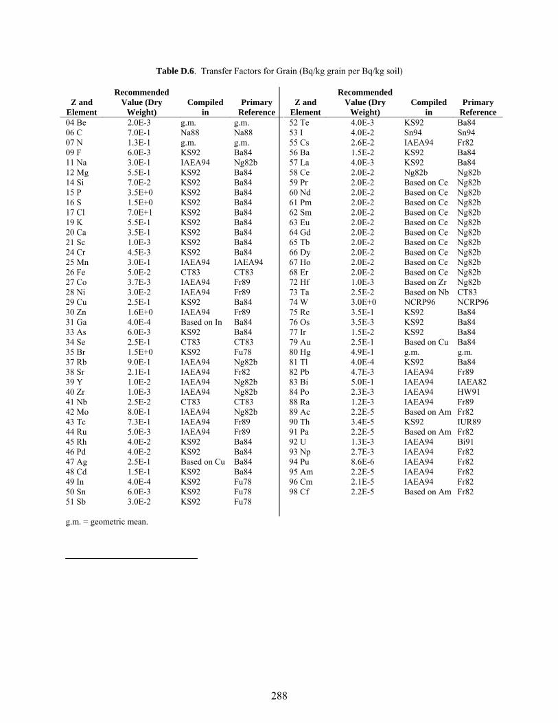
288

Table D.6. Transfer Factors for Grain (Bq/kg grain per Bq/kg soil)

Z and Element

Recommended Value (Dry

Weight) Compiled

in Primary

Reference 04 Be 2.0E-3 g.m. g.m. 06 C 7.0E-1 Na88 Na88 07 N 1.3E-1 g.m. g.m. 09 F 6.0E-3 KS92 Ba84 11 Na 3.0E-1 IAEA94 Ng82b 12 Mg 5.5E-1 KS92 Ba84 14 Si 7.0E-2 KS92 Ba84 15 P 3.5E+0 KS92 Ba84 16 S 1.5E+0 KS92 Ba84 17 Cl 7.0E+1 KS92 Ba84 19 K 5.5E-1 KS92 Ba84 20 Ca 3.5E-1 KS92 Ba84 21 Sc 1.0E-3 KS92 Ba84 24 Cr 4.5E-3 KS92 Ba84 25 Mn 3.0E-1 IAEA94 IAEA94 26 Fe 5.0E-2 CT83 CT83 27 Co 3.7E-3 IAEA94 Fr89 28 Ni 3.0E-2 IAEA94 Fr89 29 Cu 2.5E-1 KS92 Ba84 30 Zn 1.6E+0 IAEA94 Fr89 31 Ga 4.0E-4 Based on In Ba84 33 As 6.0E-3 KS92 Ba84 34 Se 2.5E-1 CT83 CT83 35 Br 1.5E+0 KS92 Fu78 37 Rb 9.0E-1 IAEA94 Ng82b 38 Sr 2.1E-1 IAEA94 Fr82 39 Y 1.0E-2 IAEA94 Ng82b 40 Zr 1.0E-3 IAEA94 Ng82b 41 Nb 2.5E-2 CT83 CT83 42 Mo 8.0E-1 IAEA94 Ng82b 43 Tc 7.3E-1 IAEA94 Fr89 44 Ru 5.0E-3 IAEA94 Fr89 45 Rh 4.0E-2 KS92 Ba84 46 Pd 4.0E-2 KS92 Ba84 47 Ag 2.5E-1 Based on Cu Ba84 48 Cd 1.5E-1 KS92 Ba84 49 In 4.0E-4 KS92 Fu78 50 Sn 6.0E-3 KS92 Fu78 51 Sb 3.0E-2 KS92 Fu78

Z and Element

Recommended Value (Dry

Weight) Compiled

in Primary

Reference 52 Te 4.0E-3 KS92 Ba84 53 I 4.0E-2 Sn94 Sn94 55 Cs 2.6E-2 IAEA94 Fr82 56 Ba 1.5E-2 KS92 Ba84 57 La 4.0E-3 KS92 Ba84 58 Ce 2.0E-2 Ng82b Ng82b 59 Pr 2.0E-2 Based on Ce Ng82b 60 Nd 2.0E-2 Based on Ce Ng82b 61 Pm 2.0E-2 Based on Ce Ng82b 62 Sm 2.0E-2 Based on Ce Ng82b 63 Eu 2.0E-2 Based on Ce Ng82b 64 Gd 2.0E-2 Based on Ce Ng82b 65 Tb 2.0E-2 Based on Ce Ng82b 66 Dy 2.0E-2 Based on Ce Ng82b 67 Ho 2.0E-2 Based on Ce Ng82b 68 Er 2.0E-2 Based on Ce Ng82b 72 Hf 1.0E-3 Based on Zr Ng82b 73 Ta 2.5E-2 Based on Nb CT83 74 W 3.0E+0 NCRP96 NCRP96 75 Re 3.5E-1 KS92 Ba84 76 Os 3.5E-3 KS92 Ba84 77 Ir 1.5E-2 KS92 Ba84 79 Au 2.5E-1 Based on Cu Ba84 80 Hg 4.9E-1 g.m. g.m. 81 Tl 4.0E-4 KS92 Ba84 82 Pb 4.7E-3 IAEA94 Fr89 83 Bi 5.0E-1 IAEA94 IAEA82 84 Po 2.3E-3 IAEA94 HW91 88 Ra 1.2E-3 IAEA94 Fr89 89 Ac 2.2E-5 Based on Am Fr82 90 Th 3.4E-5 KS92 IUR89 91 Pa 2.2E-5 Based on Am Fr82 92 U 1.3E-3 IAEA94 Bi91 93 Np 2.7E-3 IAEA94 Fr82 94 Pu 8.6E-6 IAEA94 Fr82 95 Am 2.2E-5 IAEA94 Fr82 96 Cm 2.1E-5 IAEA94 Fr82 98 Cf 2.2E-5 Based on Am Fr82

g.m. = geometric mean.

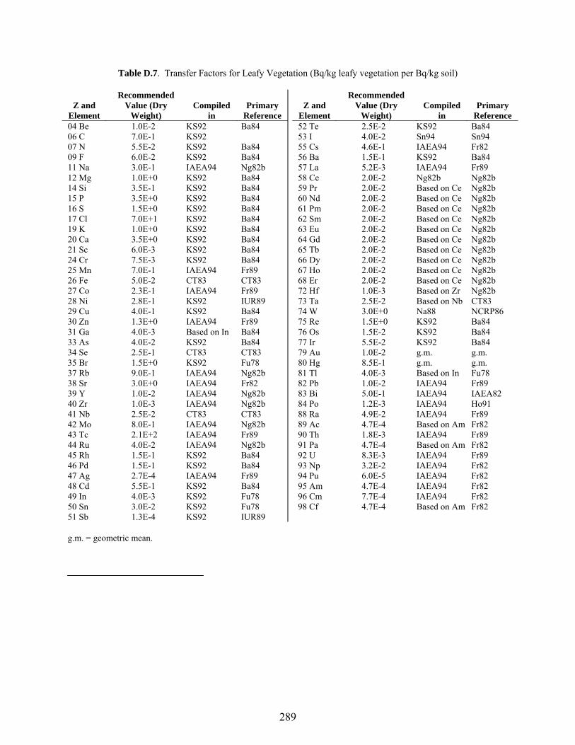
289

Table D.7. Transfer Factors for Leafy Vegetation (Bq/kg leafy vegetation per Bq/kg soil)

Z and Element

Recommended Value (Dry

Weight) Compiled

in Primary

Reference 04 Be 1.0E-2 KS92 Ba84 06 C 7.0E-1 KS92 07 N 5.5E-2 KS92 Ba84 09 F 6.0E-2 KS92 Ba84 11 Na 3.0E-1 IAEA94 Ng82b 12 Mg 1.0E+0 KS92 Ba84 14 Si 3.5E-1 KS92 Ba84 15 P 3.5E+0 KS92 Ba84 16 S 1.5E+0 KS92 Ba84 17 Cl 7.0E+1 KS92 Ba84 19 K 1.0E+0 KS92 Ba84 20 Ca 3.5E+0 KS92 Ba84 21 Sc 6.0E-3 KS92 Ba84 24 Cr 7.5E-3 KS92 Ba84 25 Mn 7.0E-1 IAEA94 Fr89 26 Fe 5.0E-2 CT83 CT83 27 Co 2.3E-1 IAEA94 Fr89 28 Ni 2.8E-1 KS92 IUR89 29 Cu 4.0E-1 KS92 Ba84 30 Zn 1.3E+0 IAEA94 Fr89 31 Ga 4.0E-3 Based on In Ba84 33 As 4.0E-2 KS92 Ba84 34 Se 2.5E-1 CT83 CT83 35 Br 1.5E+0 KS92 Fu78 37 Rb 9.0E-1 IAEA94 Ng82b 38 Sr 3.0E+0 IAEA94 Fr82 39 Y 1.0E-2 IAEA94 Ng82b 40 Zr 1.0E-3 IAEA94 Ng82b 41 Nb 2.5E-2 CT83 CT83 42 Mo 8.0E-1 IAEA94 Ng82b 43 Tc 2.1E+2 IAEA94 Fr89 44 Ru 4.0E-2 IAEA94 Ng82b 45 Rh 1.5E-1 KS92 Ba84 46 Pd 1.5E-1 KS92 Ba84 47 Ag 2.7E-4 IAEA94 Fr89 48 Cd 5.5E-1 KS92 Ba84 49 In 4.0E-3 KS92 Fu78 50 Sn 3.0E-2 KS92 Fu78 51 Sb 1.3E-4 KS92 IUR89

Z and Element

Recommended Value (Dry

Weight) Compiled

in Primary

Reference 52 Te 2.5E-2 KS92 Ba84 53 I 4.0E-2 Sn94 Sn94 55 Cs 4.6E-1 IAEA94 Fr82 56 Ba 1.5E-1 KS92 Ba84 57 La 5.2E-3 IAEA94 Fr89 58 Ce 2.0E-2 Ng82b Ng82b 59 Pr 2.0E-2 Based on Ce Ng82b 60 Nd 2.0E-2 Based on Ce Ng82b 61 Pm 2.0E-2 Based on Ce Ng82b 62 Sm 2.0E-2 Based on Ce Ng82b 63 Eu 2.0E-2 Based on Ce Ng82b 64 Gd 2.0E-2 Based on Ce Ng82b 65 Tb 2.0E-2 Based on Ce Ng82b 66 Dy 2.0E-2 Based on Ce Ng82b 67 Ho 2.0E-2 Based on Ce Ng82b 68 Er 2.0E-2 Based on Ce Ng82b 72 Hf 1.0E-3 Based on Zr Ng82b 73 Ta 2.5E-2 Based on Nb CT83 74 W 3.0E+0 Na88 NCRP86 75 Re 1.5E+0 KS92 Ba84 76 Os 1.5E-2 KS92 Ba84 77 Ir 5.5E-2 KS92 Ba84 79 Au 1.0E-2 g.m. g.m. 80 Hg 8.5E-1 g.m. g.m. 81 Tl 4.0E-3 Based on In Fu78 82 Pb 1.0E-2 IAEA94 Fr89 83 Bi 5.0E-1 IAEA94 IAEA82 84 Po 1.2E-3 IAEA94 Ho91 88 Ra 4.9E-2 IAEA94 Fr89 89 Ac 4.7E-4 Based on Am Fr82 90 Th 1.8E-3 IAEA94 Fr89 91 Pa 4.7E-4 Based on Am Fr82 92 U 8.3E-3 IAEA94 Fr89 93 Np 3.2E-2 IAEA94 Fr82 94 Pu 6.0E-5 IAEA94 Fr82 95 Am 4.7E-4 IAEA94 Fr82 96 Cm 7.7E-4 IAEA94 Fr82 98 Cf 4.7E-4 Based on Am Fr82

g.m. = geometric mean.

290

Table D.8. Transfer Factors for Milk (Bq/L milk per Bq/d intake)

Z and Element

Recommended Value (Wet

Weight) Compiled

in Primary

Reference 01 H 1.5E-2 IAEA94 Va83 04 Be 9.0E-7 KS92 Ng77 07 N 2.5E-2 KS92 Ng77 09 F 1.0E-3 KS92 Ng77 11 Na 1.6E-2 IAEA94 IAEA94 12 Mg 3.9E-3 IAEA94 Ng82a 14 Si 2.0E-5 KS92 Ng77 15 P 1.6E-2 IAEA94 Ng82a 16 S 1.6E-2 IAEA94 Ng82a 17 Cl 1.7E-2 IAEA94 Bi89 19 K 7.2E-3 IAEA94 Ng82a 20 Ca 3.0E-3 IAEA94 CT83 21 Sc 5.0E-6 KS92 Ng77 24 Cr 1.0E-5 IAEA94 Va84 25 Mn 3.0E-5 IAEA94 Va84 26 Fe 3.0E-5 IAEA94 Va84 27 Co 3.0E-4 IAEA94 Ba84 28 Ni 1.6E-2 IAEA94 Cr90 29 Cu 2.0E-3 Na88 IAEA87 30 Zn 1.0E-2 KS92 Ng77 31 Ga 5.0E-5 KS92 Ng77 33 As 6.0E-5 KS92 Ng77 34 Se 4.0E-3 KS92 Ng77 35 Br 2.0E-2 KS92 Ng77 37 Rb 1.2E-2 IAEA94 Ng82a 38 Sr 2.8E-3 IAEA94 Co90 39 Y 2.0E-5 KS92 Ng77 40 Zr 5.5E-7 IAEA94 Jo88 41 Nb 4.1E-7 IAEA94 Jo88 42 Mo 1.7E-3 IAEA94 Jo88 43 Tc 1.4E-4 IAEA94 Jo88 44 Ru 3.3E-6 IAEA94 Co90 45 Rh 1.0E-2 KS92 Ng77 46 Pd 1.0E-2 KS92 Ng77 47 Ag 5.0E-5 IAEA94 CEC87 48 Cd 1.0E-3 KS92 Ng77 49 In 2.0E-4 Na88 NCRP86 50 Sn 1.0E-3 Na88 NCRP86 51 Sb 2.5E-5 IAEA94 Va82

Z and Element

Recommended Value (Wet

Weight) Compiled

in Primary

Reference 52 Te 4.5E-4 IAEA94 Jo88 53 I 9.0E-3 Sn94 Sn94 55 Cs 7.9E-3 IAEA94 Co90 56 Ba 4.8E-4 IAEA94 Jo88 57 La 2.0E-5 KS92 Ng77 58 Ce 3.0E-5 IAEA94 CEC87 59 Pr 3.0E-5 Based on Ce CEC87 60 Nd 3.0E-5 Based on Ce CEC87 61 Pm 3.0E-5 Based on Ce CEC87 62 Sm 3.0E-5 Based on Ce CEC87 63 Eu 3.0E-5 Based on Ce CEC87 64 Gd 3.0E-5 Based on Ce CEC87 65 Tb 3.0E-5 Based on Ce CEC87 66 Dy 3.0E-5 Based on Ce CEC87 67 Ho 3.0E-5 Based on Ce CEC87 68 Er 3.0E-5 Based on Ce CEC87 72 Hf 5.5E-7 Based on Zr Jo88 73 Ta 4.1E-7 Based on Nb Jo88 74 W 3.0E-4 KS92 Ng77 75 Re 1.5E-3 KS92 Ng77 76 Os 5.0E-3 KS92 Ng77 77 Ir 2.0E-6 KS92 Ng77 79 Au 5.5E-6 KS92 Ng77 80 Hg 4.7E-4 IAEA94 Ng82a 81 Tl 2.0E-3 Na88 Na88 82 Pb 2.6E-4 KS92 Ng77 83 Bi 5.0E-4 KS92 Ng77 84 Po 3.4E-4 IAEA94 Ng82a 88 Ra 1.3E-3 IAEA94 MB90 89 Ac 2.0E-5 KS92 Ng77 90 Th 5.0E-6 KS92 Ng77 91 Pa 5.0E-6 KS92 Ng77 92 U 4.0E-4 IAEA94 MB90 93 Np 5.0E-6 IAEA94 Ng82a 94 Pu 1.1E-6 IAEA94 Co90 95 Am 1.5E-6 IAEA94 Co90 96 Cm 2.0E-5 KS92 Ng77 98 Cf 1.5E-6 Based on Am Co90

g.m. = geometric mean.

291

Table D.9. Transfer Factors for Poultry (Bq/kg poultry muscle per Bq/d intake)

Z and Element

Recommended Value (Wet

Weight) Compiled

in Primary

Reference 04 Be 4.0E-1 KS92 Na88 07 N 9.8E-2 g.m. g.m. 09 F 1.4E-2 g.m. g.m. 11 Na 1.0E-2 KS92 Na88 12 Mg 3.0E-2 KS92 KS92 14 Si 8.0E-1 Based on As Na88 15 P 1.9E-1 KS92 Na88 16 S 2.3E+0 g.m. g.m. 17 Cl 3.0E-2 KS92 Na88 19 K 4.0E-1 KS92 KS92 20 Ca 4.0E-2 IAEA94 Ng82a 21 Sc 4.0E-3 KS92 Na88 24 Cr 2.0E-1 KS92 KS92 25 Mn 5.0E-2 IAEA94 Ng82a 26 Fe 1.0E+0 IAEA94 Ng82a 27 Co 2.0E+0 IAEA94 Ng82a 28 Ni 1.0E-3 KS92 Na88 29 Cu 5.0E-1 IAEA94 Ng82a 30 Zn 7.0E+0 IAEA94 Ng82a 31 Ga 8.0E-1 Based on As Na88 33 As 8.3E-1 KS92 Na88 34 Se 9.0E+0 IAEA94 Ng82a 35 Br 4.0E-3 KS92 Na88 37 Rb 2.0E+0 KS92 Na88 38 Sr 8.0E-2 IAEA94 Co90 39 Y 1.0E-2 IAEA94 Ng82a 40 Zr 6.0E-5 IAEA94 En88a 41 Nb 3.0E-4 IAEA94 En88a 42 Mo 1.8E-1 En88a En88a 43 Tc 3.0E-2 IAEA94 En88b 44 Ru 7.0E-3 Na88 Ng82a 45 Rh 2.0E+0 Based on Co Ng82a 46 Pd 3.0E-4 KS92 Na88 47 Ag 2.0E+0 IAEA94 CEC87 48 Cd 8.0E-1 IAEA94 Ng82a 49 In 8.0E-1 Based on As Na88 50 Sn 8.0E-1 Based on As Na88 51 Sb 6.0E-3 Na88 Na88

Z and Element

Recommended Value (Wet

Weight) Compiled

in Primary

Reference 52 Te 6.0E-1 IAEA94 En88a 53 I 5.0E-2 Sn94 Sn94 55 Cs 3.0E+0 Vo93 Vo93 56 Ba 9.0E-3 IAEA94 En88a 57 La 1.0E-1 IAEA94 Ng82a 58 Ce 2.0E-3 IAEA94 Ng82a 59 Pr 2.0E-3 Based on Ce Ng82a 60 Nd 2.0E-3 Based on Ce Ng82a 61 Pm 2.0E-3 Based on Ce Ng82a 62 Sm 2.0E-3 Based on Ce Ng82a 63 Eu 2.0E-3 Based on Ce Ng82a 64 Gd 2.0E-3 Based on Ce Ng82a 65 Tb 2.0E-3 Based on Ce Ng82a 66 Dy 2.0E-3 Based on Ce Ng82a 67 Ho 2.0E-3 Based on Ce Ng82a 68 Er 2.0E-3 Based on Ce Ng82a 72 Hf 6.0E-5 based on Zr En88a 73 Ta 3.0E-4 Based on Nb En88a 74 W 2.0E-1 Based on Mo IAEA94 75 Re 4.0E-2 KS92 Ba84 76 Os 8.4E-2 g.m. g.m. 77 Ir 2.0E+0 Based on Co Ng82a 79 Au 1.0E+0 g.m. g.m. 80 Hg 3.0E-2 IAEA94 Ng82a 81 Tl 8.0E-1 Based on In Na88 82 Pb 8.0E-1 Based on As Na88 83 Bi 9.8E-2 g.m. g.m. 84 Po 2.3E+0 g.m. g.m. 88 Ra 3.0E-2 KS92 KS92 89 Ac 6.0E-3 Based on Am Co90 90 Th 6.0E-3 Based on Am Co90 91 Pa 6.0E-3 Based on Am Co90 92 U 1.0E+0 IAEA94 Ng82a 93 Np 6.0E-3 Based on Am Co90 94 Pu 3.0E-3 IAEA94 Co90 95 Am 6.0E-3 IAEA94 Co90 96 Cm 6.0E-3 Based on Am Co90 98 Cf 6.0E-3 Based on Am Co90

g.m. = geometric mean.

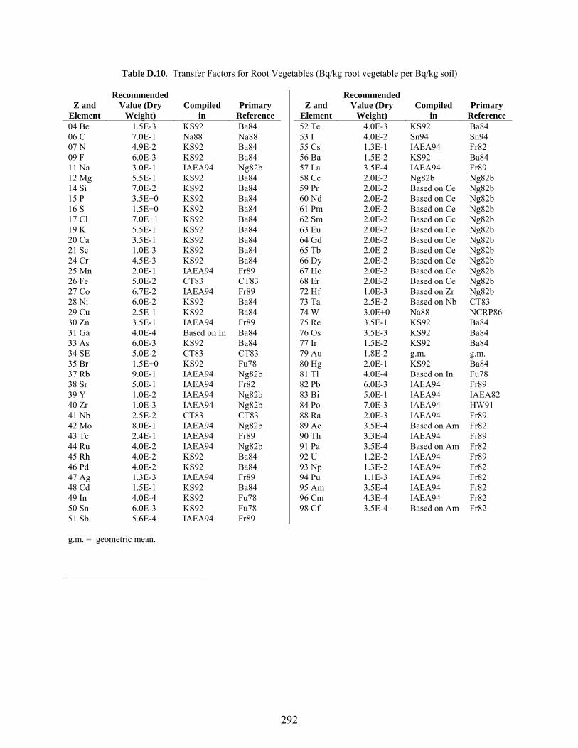
292

Table D.10. Transfer Factors for Root Vegetables (Bq/kg root vegetable per Bq/kg soil)

Z and Element

Recommended Value (Dry

Weight) Compiled

in Primary

Reference 04 Be 1.5E-3 KS92 Ba84 06 C 7.0E-1 Na88 Na88 07 N 4.9E-2 KS92 Ba84 09 F 6.0E-3 KS92 Ba84 11 Na 3.0E-1 IAEA94 Ng82b 12 Mg 5.5E-1 KS92 Ba84 14 Si 7.0E-2 KS92 Ba84 15 P 3.5E+0 KS92 Ba84 16 S 1.5E+0 KS92 Ba84 17 Cl 7.0E+1 KS92 Ba84 19 K 5.5E-1 KS92 Ba84 20 Ca 3.5E-1 KS92 Ba84 21 Sc 1.0E-3 KS92 Ba84 24 Cr 4.5E-3 KS92 Ba84 25 Mn 2.0E-1 IAEA94 Fr89 26 Fe 5.0E-2 CT83 CT83 27 Co 6.7E-2 IAEA94 Fr89 28 Ni 6.0E-2 KS92 Ba84 29 Cu 2.5E-1 KS92 Ba84 30 Zn 3.5E-1 IAEA94 Fr89 31 Ga 4.0E-4 Based on In Ba84 33 As 6.0E-3 KS92 Ba84 34 SE 5.0E-2 CT83 CT83 35 Br 1.5E+0 KS92 Fu78 37 Rb 9.0E-1 IAEA94 Ng82b 38 Sr 5.0E-1 IAEA94 Fr82 39 Y 1.0E-2 IAEA94 Ng82b 40 Zr 1.0E-3 IAEA94 Ng82b 41 Nb 2.5E-2 CT83 CT83 42 Mo 8.0E-1 IAEA94 Ng82b 43 Tc 2.4E-1 IAEA94 Fr89 44 Ru 4.0E-2 IAEA94 Ng82b 45 Rh 4.0E-2 KS92 Ba84 46 Pd 4.0E-2 KS92 Ba84 47 Ag 1.3E-3 IAEA94 Fr89 48 Cd 1.5E-1 KS92 Ba84 49 In 4.0E-4 KS92 Fu78 50 Sn 6.0E-3 KS92 Fu78 51 Sb 5.6E-4 IAEA94 Fr89

Z and Element

Recommended Value (Dry

Weight) Compiled

in Primary

Reference 52 Te 4.0E-3 KS92 Ba84 53 I 4.0E-2 Sn94 Sn94 55 Cs 1.3E-1 IAEA94 Fr82 56 Ba 1.5E-2 KS92 Ba84 57 La 3.5E-4 IAEA94 Fr89 58 Ce 2.0E-2 Ng82b Ng82b 59 Pr 2.0E-2 Based on Ce Ng82b 60 Nd 2.0E-2 Based on Ce Ng82b 61 Pm 2.0E-2 Based on Ce Ng82b 62 Sm 2.0E-2 Based on Ce Ng82b 63 Eu 2.0E-2 Based on Ce Ng82b 64 Gd 2.0E-2 Based on Ce Ng82b 65 Tb 2.0E-2 Based on Ce Ng82b 66 Dy 2.0E-2 Based on Ce Ng82b 67 Ho 2.0E-2 Based on Ce Ng82b 68 Er 2.0E-2 Based on Ce Ng82b 72 Hf 1.0E-3 Based on Zr Ng82b 73 Ta 2.5E-2 Based on Nb CT83 74 W 3.0E+0 Na88 NCRP86 75 Re 3.5E-1 KS92 Ba84 76 Os 3.5E-3 KS92 Ba84 77 Ir 1.5E-2 KS92 Ba84 79 Au 1.8E-2 g.m. g.m. 80 Hg 2.0E-1 KS92 Ba84 81 Tl 4.0E-4 Based on In Fu78 82 Pb 6.0E-3 IAEA94 Fr89 83 Bi 5.0E-1 IAEA94 IAEA82 84 Po 7.0E-3 IAEA94 HW91 88 Ra 2.0E-3 IAEA94 Fr89 89 Ac 3.5E-4 Based on Am Fr82 90 Th 3.3E-4 IAEA94 Fr89 91 Pa 3.5E-4 Based on Am Fr82 92 U 1.2E-2 IAEA94 Fr89 93 Np 1.3E-2 IAEA94 Fr82 94 Pu 1.1E-3 IAEA94 Fr82 95 Am 3.5E-4 IAEA94 Fr82 96 Cm 4.3E-4 IAEA94 Fr82 98 Cf 3.5E-4 Based on Am Fr82

g.m. = geometric mean.

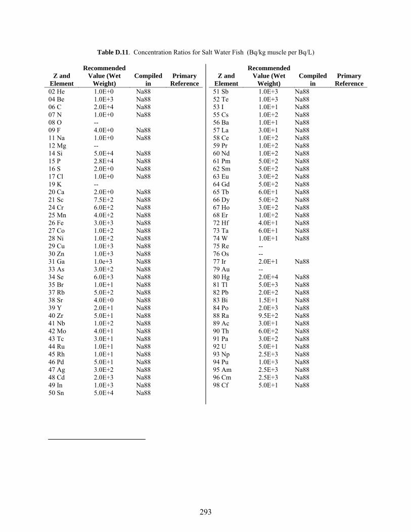
293

Table D.11. Concentration Ratios for Salt Water Fish (Bq/kg muscle per Bq/L)

Z and Element

Recommended Value (Wet

Weight) Compiled

in Primary

Reference 02 He 1.0E+0 Na88 04 Be 1.0E+3 Na88 06 C 2.0E+4 Na88 07 N 1.0E+0 Na88 08 O -- 09 F 4.0E+0 Na88 11 Na 1.0E+0 Na88 12 Mg -- 14 Si 5.0E+4 Na88 15 P 2.8E+4 Na88 16 S 2.0E+0 Na88 17 Cl 1.0E+0 Na88 19 K -- 20 Ca 2.0E+0 Na88 21 Sc 7.5E+2 Na88 24 Cr 6.0E+2 Na88 25 Mn 4.0E+2 Na88 26 Fe 3.0E+3 Na88 27 Co 1.0E+2 Na88 28 Ni 1.0E+2 Na88 29 Cu 1.0E+3 Na88 30 Zn 1.0E+3 Na88 31 Ga 1.0e+3 Na88 33 As 3.0E+2 Na88 34 Se 6.0E+3 Na88 35 Br 1.0E+1 Na88 37 Rb 5.0E+2 Na88 38 Sr 4.0E+0 Na88 39 Y 2.0E+1 Na88 40 Zr 5.0E+1 Na88 41 Nb 1.0E+2 Na88 42 Mo 4.0E+1 Na88 43 Tc 3.0E+1 Na88 44 Ru 1.0E+1 Na88 45 Rh 1.0E+1 Na88 46 Pd 5.0E+1 Na88 47 Ag 3.0E+2 Na88 48 Cd 2.0E+3 Na88 49 In 1.0E+3 Na88 50 Sn 5.0E+4 Na88

Z and Element

Recommended Value (Wet

Weight) Compiled

in Primary

Reference 51 Sb 1.0E+3 Na88 52 Te 1.0E+3 Na88 53 I 1.0E+1 Na88 55 Cs 1.0E+2 Na88 56 Ba 1.0E+1 Na88 57 La 3.0E+1 Na88 58 Ce 1.0E+2 Na88 59 Pr 1.0E+2 Na88 60 Nd 1.0E+2 Na88 61 Pm 5.0E+2 Na88 62 Sm 5.0E+2 Na88 63 Eu 3.0E+2 Na88 64 Gd 5.0E+2 Na88 65 Tb 6.0E+1 Na88 66 Dy 5.0E+2 Na88 67 Ho 3.0E+2 Na88 68 Er 1.0E+2 Na88 72 Hf 4.0E+1 Na88 73 Ta 6.0E+1 Na88 74 W 1.0E+1 Na88 75 Re -- 76 Os -- 77 Ir 2.0E+1 Na88 79 Au -- 80 Hg 2.0E+4 Na88 81 Tl 5.0E+3 Na88 82 Pb 2.0E+2 Na88 83 Bi 1.5E+1 Na88 84 Po 2.0E+3 Na88 88 Ra 9.5E+2 Na88 89 Ac 3.0E+1 Na88 90 Th 6.0E+2 Na88 91 Pa 3.0E+2 Na88 92 U 5.0E+1 Na88 93 Np 2.5E+3 Na88 94 Pu 1.0E+3 Na88 95 Am 2.5E+3 Na88 96 Cm 2.5E+3 Na88 98 Cf 5.0E+1 Na88

294

Table D.12. Concentration Ratios for Crustaceans (Bq/kg muscle per Bq/L [wet])

Z and Element Salt Water

Fresh Water

Compiled in

02 He 1.0E+0 1.0E+0 Na88 04 Be 1.0E+4 5.0E+1 Na88 06 C 2.0E+4 9.0E+3 Na88 07 N 1.0E+0 1.0E+0 Na88 08 O -- -- Na88 09 F 4.0E+0 1.0E+2 Na88 11 Na 1.0E-0 1.0E+2 Na88 12 Mg -- -- 14 Si 5.0E+4 1.0E+4 Na88 15 P 3.8E+4 1.0E+5 Na88 16 S 1.0E+0 1.0E+2 Na88 17 Cl 1.0E+0 5.0E+1 Na88 19 K -- -- Na88 20 Ca 5.0E+0 2.0E+3 Na88 21 Sc 3.0E+2 1.0E+3 Na88 24 Cr 5.0E+2 2.0E+3 Na88 25 Mn 8.0E+2 1.0E+5 Na88 26 Fe 5.0E+3 1.0E+2 Na88 27 Co 2.0E+3 2.0E+3 Na88 28 Ni 5.0E+2 5.0E+2 Na88 29 Cu 5.0E+3 4.0E+2 Na88 30 Zn 5.0E+4 1.0E+4 Na88 31 Ga 1.0E+4 1.0E+4 Na88 33 As 3.0E+2 3.0E+2 Na88 34 Se 5.0E+3 2.0E+3 Na88 35 Br 1.0E+1 3.3E+2 Na88 37 Rb 2.0E+2 1.0E+3 Na88 38 Sr 1.0E+0 1.0E+2 Na88 39 Y 1.0E+3 1.0E+3 Na88 40 Zr 5.0E+1 5.0E+1 Na88 41 Nb 5.0E+1 5.0E+1 Na88 42 Mo 2.0E+1 1.0E+2 Na88 43 Tc 1.0E+1 1.0E+2 Na88 44 Ru 1.0E+2 3.0E+2 Na88 45 Rh 1.0E+2 3.0E+2 Na88 46 Pd 3.0E+2 2.0E+3 Na88 47 Ag 3.5E+2 2.0E+2 Na88 48 Cd 5.0E+3 1.0E+4 Na88 49 In 1.0E+4 1.0E+4 Na88 50 Sn 5.0E+4 1.0E+4 Na88

Z and Element Salt Water

Fresh Water

Compiled in

51 Sb 1.0E+2 1.0E+2 Na88 52 Te 1.0E+3 6.1E+3 Na88 53 I 5.0E+1 1.0E+2 Na88 55 Cs 3.0E+1 5.0E+2 Na88 56 Ba 1.0E+0 2.0E+2 Na88 57 La 1.0E+2 1.0E+3 Na88 58 Ce 5.0E+2 1.0E+3 Na88 59 Pr 1.0E+3 1.0E+3 Na88 60 Nd -- Na88 61 Pm 1.0E+3 3.0E+3 Na88 62 Sm 1.0E+3 3.0E+3 Na88 63 Eu 1.0E+3 3.0E+3 Na88 64 Gd 2.0E+3 2.0E+3 Na88 65 Tb 1.0E+3 1.0E+3 Na88 66 Dy 1.0E+3 1.0E+3 Na88 67 Ho 1.0E+3 3.0E+3 Na88 68 Er 5.0E+2 1.0E+3 Na88 72 Hf 1.0E+3 1.0E+3 Na88 73 Ta 3.0E+3 3.0E+3 Na88 74 W 1.0E+1 1.0E+1 Na88 75 Re -- -- 76 Os -- -- 77 Ir 1.0E+2 2.0E+2 Na88 79 Au -- -- 80 Hg 2.0E+4 2.0E+4 Na88 81 Tl 1.0E+3 1.0E+3 Na88 82 Pb 1.0E+3 5.0E+2 Na88 83 Bi 1.0E+3 1.0E+5 Na88 84 Po 5.0E+4 2.0E+4 Na88 88 Ra 1.0E+2 1.0E+3 Na88 89 Ac 1.0E+3 1.0E+3 Na88 90 Th 1.0E+3 1.0E+2 Na88 91 Pa 1.0E+1 3.0E+1 Na88 92 U 1.0E+1 1.0E+2 Na88 93 Np 1.0E+1 3.0E+1 Na88 94 Pu 3.0E+2 1.0E+2 Na88 95 Am 3.6E+2 1.0E+2 Na88 96 Cm 4.6E+2 1.0E+3 Na88 98 Cf 5.0E+2 1.0E+3 Na88

295

Table D.13. Concentration Ratios for Molluscs (Bq/kg muscle per Bq/L [wet])

Z and Element Salt Water

Fresh Water

Compiled in

02 He 1.0E+0 1.0E+0 Na88 04 Be 1.0E+4 5.0E+1 Na88 06 C 2.0E+4 9.0E+3 Na88 07 N 1.0E+0 1.0E+0 Na88 08 O -- -- Na88 09 F 4.0E+0 1.0E+2 Na88 11 Na 3.0E-0 1.0E+2 Na88 12 Mg -- -- 14 Si 5.0E+4 1.0E+4 Na88 15 P 4.5E+4 1.0E+5 Na88 16 S 4.0E+0 1.0E+2 Na88 17 Cl 1.0E+0 5.0E+1 Na88 19 K -- -- Na88 20 Ca 1.0E+0 2.0E+3 Na88 21 Sc 1.0E+2 1.0E+3 Na88 24 Cr 1.1E+3 2.0E+3 Na88 25 Mn 6.0E+3 1.0E+5 Na88 26 Fe 3.0E+4 1.0E+2 Na88 27 Co 3.0E+3 2.0E+3 Na88 28 Ni 5.0E+2 5.0E+2 Na88 29 Cu 5.0E+3 4.0E+2 Na88 30 Zn 3.0E+4 1.0E+4 Na88 31 Ga 1.0E+4 1.0E+4 Na88 33 As 3.0E+2 3.0E+2 Na88 34 Se 6.0E+3 2.0E+3 Na88 35 Br 1.0E+1 3.3E+2 Na88 37 Rb 2.0E+2 1.0E+3 Na88 38 Sr 4.0E+1 1.0E+2 Na88 39 Y 1.0E+3 1.0E+3 Na88 40 Zr 5.0E+1 5.0E+1 Na88 41 Nb 5.0E+1 5.0E+1 Na88 42 Mo 2.0E+1 1.0E+2 Na88 43 Tc 2.0E+1 1.0E+2 Na88 44 Ru 2.0E+3 3.0E+2 Na88 45 Rh 1.0E+2 3.0E+2 Na88 46 Pd 3.0E+2 2.0E+3 Na88 47 Ag 5.8E+2 2.0E+2 Na88 48 Cd 1.0E+4 1.0E+4 Na88 49 In 1.0E+4 1.0E+4 Na88 50 Sn 5.0E+4 1.0E+4 Na88

Z and Element Salt Water

Fresh Water

Compiled in

51 Sb 1.2E+3 1.0E+2 Na88 52 Te 1.0E+3 6.1E+3 Na88 53 I 5.0E+1 1.0E+2 Na88 55 Cs 3.0E+1 5.0E+2 Na88 56 Ba 2.0E+1 2.0E+2 Na88 57 La 1.0E+2 1.0E+3 Na88 58 Ce 5.0E+2 1.0E+3 Na88 59 Pr 1.0E+3 1.0E+3 Na88 60 Nd -- -- Na88 61 Pm 5.0E+3 3.0E+3 Na88 62 Sm 5.0E+3 3.0E+3 Na88 63 Eu 7.0E+3 3.0E+3 Na88 64 Gd 5.0E+3 5.0E+3 Na88 65 Tb 3.0E+3 1.0E+3 Na88 66 Dy 5.0E+3 5.0E+3 Na88 67 Ho 1.0E+3 3.0E+3 Na88 68 Er 5.0E+2 1.0E+3 Na88 72 Hf 3.0E+3 3.0E+3 Na88 73 Ta 3.0E+3 3.0E+3 Na88 74 W 1.0E+2 1.0E+1 Na88 75 Re -- -- 76 Os -- -- 77 Ir 1.0E+2 2.0E+2 Na88 79 Au -- -- 80 Hg 1.0E+4 2.0E+4 Na88 81 Tl 5.0E+3 5.0E+3 Na88 82 Pb 1.0E+3 5.0E+2 Na88 83 Bi 1.0E+3 1.0E+5 Na88 84 Po 1.0E+4 2.0E+4 Na88 88 Ra 1.0E+2 1.0E+3 Na88 89 Ac 1.0E+3 1.0E+3 Na88 90 Th 1.0E+3 1.0E+2 Na88 91 Pa 1.0E+1 3.0E+1 Na88 92 U 3.0E+1 1.0E+2 Na88 93 Np 1.5E+2 3.0E+1 Na88 94 Pu 3.0E+3 1.0E+2 Na88 95 Am 2.9E+2 1.0E+2 Na88 96 Cm 4.6E+2 1.0E+3 Na88 98 Cf 2.0E+3 1.0E+3 Na88

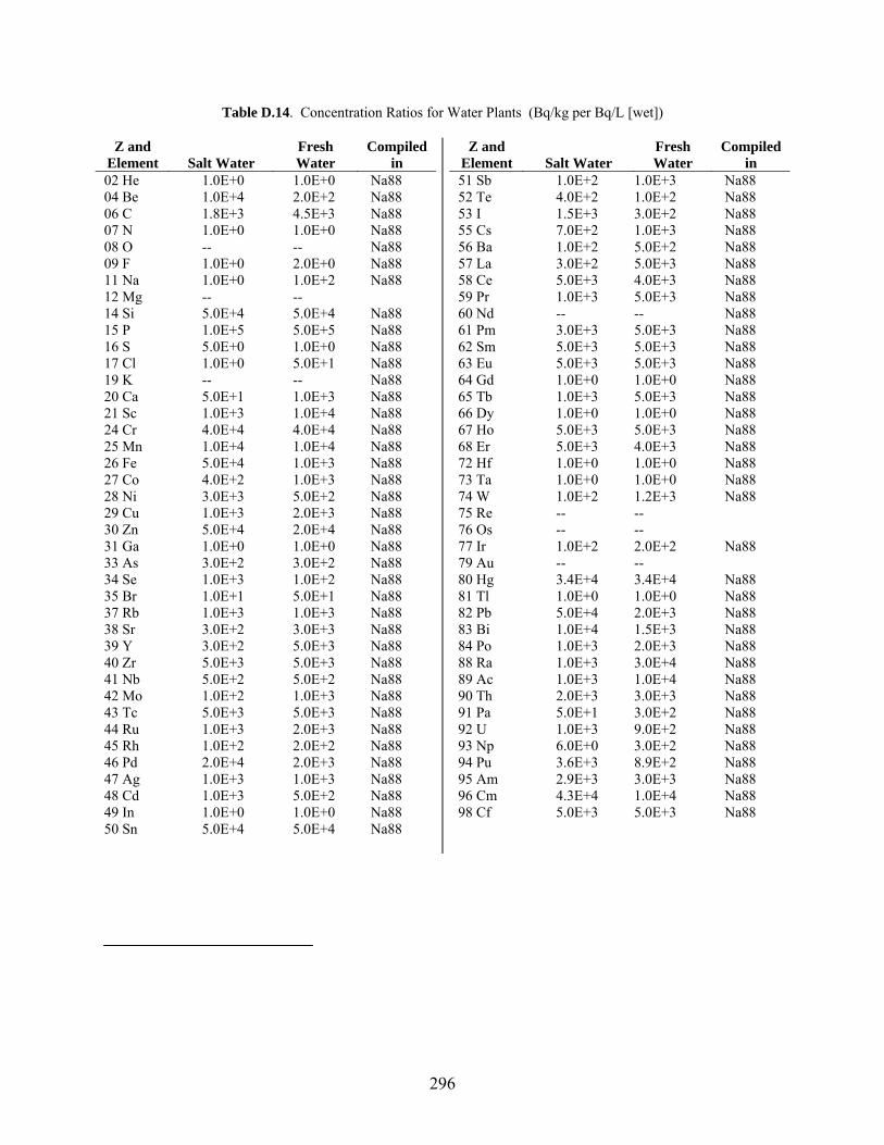
296

Table D.14. Concentration Ratios for Water Plants (Bq/kg per Bq/L [wet])

Z and Element Salt Water

Fresh Water

Compiled in

02 He 1.0E+0 1.0E+0 Na88 04 Be 1.0E+4 2.0E+2 Na88 06 C 1.8E+3 4.5E+3 Na88 07 N 1.0E+0 1.0E+0 Na88 08 O -- -- Na88 09 F 1.0E+0 2.0E+0 Na88 11 Na 1.0E+0 1.0E+2 Na88 12 Mg -- -- 14 Si 5.0E+4 5.0E+4 Na88 15 P 1.0E+5 5.0E+5 Na88 16 S 5.0E+0 1.0E+0 Na88 17 Cl 1.0E+0 5.0E+1 Na88 19 K -- -- Na88 20 Ca 5.0E+1 1.0E+3 Na88 21 Sc 1.0E+3 1.0E+4 Na88 24 Cr 4.0E+4 4.0E+4 Na88 25 Mn 1.0E+4 1.0E+4 Na88 26 Fe 5.0E+4 1.0E+3 Na88 27 Co 4.0E+2 1.0E+3 Na88 28 Ni 3.0E+3 5.0E+2 Na88 29 Cu 1.0E+3 2.0E+3 Na88 30 Zn 5.0E+4 2.0E+4 Na88 31 Ga 1.0E+0 1.0E+0 Na88 33 As 3.0E+2 3.0E+2 Na88 34 Se 1.0E+3 1.0E+2 Na88 35 Br 1.0E+1 5.0E+1 Na88 37 Rb 1.0E+3 1.0E+3 Na88 38 Sr 3.0E+2 3.0E+3 Na88 39 Y 3.0E+2 5.0E+3 Na88 40 Zr 5.0E+3 5.0E+3 Na88 41 Nb 5.0E+2 5.0E+2 Na88 42 Mo 1.0E+2 1.0E+3 Na88 43 Tc 5.0E+3 5.0E+3 Na88 44 Ru 1.0E+3 2.0E+3 Na88 45 Rh 1.0E+2 2.0E+2 Na88 46 Pd 2.0E+4 2.0E+3 Na88 47 Ag 1.0E+3 1.0E+3 Na88 48 Cd 1.0E+3 5.0E+2 Na88 49 In 1.0E+0 1.0E+0 Na88 50 Sn 5.0E+4 5.0E+4 Na88

Z and Element Salt Water

Fresh Water

Compiled in

51 Sb 1.0E+2 1.0E+3 Na88 52 Te 4.0E+2 1.0E+2 Na88 53 I 1.5E+3 3.0E+2 Na88 55 Cs 7.0E+2 1.0E+3 Na88 56 Ba 1.0E+2 5.0E+2 Na88 57 La 3.0E+2 5.0E+3 Na88 58 Ce 5.0E+3 4.0E+3 Na88 59 Pr 1.0E+3 5.0E+3 Na88 60 Nd -- -- Na88 61 Pm 3.0E+3 5.0E+3 Na88 62 Sm 5.0E+3 5.0E+3 Na88 63 Eu 5.0E+3 5.0E+3 Na88 64 Gd 1.0E+0 1.0E+0 Na88 65 Tb 1.0E+3 5.0E+3 Na88 66 Dy 1.0E+0 1.0E+0 Na88 67 Ho 5.0E+3 5.0E+3 Na88 68 Er 5.0E+3 4.0E+3 Na88 72 Hf 1.0E+0 1.0E+0 Na88 73 Ta 1.0E+0 1.0E+0 Na88 74 W 1.0E+2 1.2E+3 Na88 75 Re -- -- 76 Os -- -- 77 Ir 1.0E+2 2.0E+2 Na88 79 Au -- -- 80 Hg 3.4E+4 3.4E+4 Na88 81 Tl 1.0E+0 1.0E+0 Na88 82 Pb 5.0E+4 2.0E+3 Na88 83 Bi 1.0E+4 1.5E+3 Na88 84 Po 1.0E+3 2.0E+3 Na88 88 Ra 1.0E+3 3.0E+4 Na88 89 Ac 1.0E+3 1.0E+4 Na88 90 Th 2.0E+3 3.0E+3 Na88 91 Pa 5.0E+1 3.0E+2 Na88 92 U 1.0E+3 9.0E+2 Na88 93 Np 6.0E+0 3.0E+2 Na88 94 Pu 3.6E+3 8.9E+2 Na88 95 Am 2.9E+3 3.0E+3 Na88 96 Cm 4.3E+4 1.0E+4 Na88 98 Cf 5.0E+3 5.0E+3 Na88

297

D.6 References (Ba84) Baes, C.F., R.D. Sharp, A.L. Sjoreen, and R.W. Shor. 1984. A Review and Analysis of Parameters for Assessing Transport of Environmentally Released Radionuclides through Agriculture. ORNL-5786, Oak Ridge National Laboratory, Oak Ridge, Tennessee. (Bi91) Bilo, M. 1991. Untersuchugen zum Transfer des durch den Reaktorunfall von Tschernobyl abgelagerten Radiocasiums vom Boden in die Pflanze. Thesis, Personal Communication w/ Zezina, N. Tubingen. (Bi89) Bishop, G.P., C.J. Beetham, and Y.S. Cuff. 1989. Review of Literature for Chlorine Technetium, Iodine and Neptunium. Nirex Radioactive Waste Disposal Safety Studies, NSS/R193, UK Nirex Ltd., Harwell, England. (Br79) Bruland, W., et al. 1979. “Transfer of organically bound radionuclides through food chains to man. Model--example with radiocobalt and vitamin B12.” In Biological Implications of Radionuclides Released from Nuclear Industries. Vol. 2, Proceedings of a Symposium. IAEA, Vienna. (CEC87) Commission of the European Communities. 1987. Radionuclide Transfer Factors of Animal Feedingstuffs and Animal Products. CEC Doc. 7682/87, Luxembourg. (CT83) Coughtrey, P.C., and M.C. Thorne. 1983. Radionuclide Distribution and Transport in Terrestrial and Aquatic Ecosystems, A Critical Review of Data. Vols. 1-6. A.A. Balkema, Rotterdam. (Co90) Coughtrey, P.J. 1990. Radioactivity Transfer to Animal Products. EUR 12608 EN, Commission on European Communities, Luxembourg. (Cr90) Cramp, T.J., Y.S. Cuff, A. Davis, and J.E. Morgan. 1990. Review of Data for Uranium, Nickel, and Cobalt. 2150-RI, Associated Nuclear Services, Ltd., Epsom, England. (En88a) Ennis, M.E., Jr., G.M. Ward, J.E. Johnson, and K.N. Boamah. 1988. “Transfer coefficients of selected radionuclides to animal products II. Hen eggs and meat.” Health Physics 54:167-170. (En88b) Ennis, M.E. Jr., J.E. Johnson, G.M. Ward, and G.M. Voigt. 1988. “A specific activity effect in the metabolism of Tc.” Health Physics 54:157-160. (Fr65) Freke, A.M. 1965. “A Model for the Approximate Calculation of Safe Rates of Discharge of Radioactive Wastes into Marine Environments,” Health Physics 13: 743-758.

298

(Fr82) Frissel, M.J. 1992. An Update of the Recommended Soil-to-Plant Transfer Factors. Eighth Report of the IUR Working Group on Soil-to-Plant Transfer Factors, IUR, Balen, Belgium. (Fr89) Frissel, M.J., and K.E. van Bergeijk. 1989. Mean Transfer Values Derived by Simple Statistical Regression Analysis. Sixth Report of IUR Working Group on Soil-to-Plant Transfer Factors, RIVM, Bilthoven, Netherlands. (Fu78) Furr, A.K., T.F. Parkinson, C.L. Heffron, J.T. Reid, W.M. Haschek, W.H. Gutenmann, C.A. Backe, L.E. St. John, Jr., and D.J. Lisk. 1979. “Elemental Content of Tissues and excreta of lambs, goats and kids fed white sweet clover growing on fly ash.” Journal of Agric. Food Chem., 26(4):847-851. (Ho91) Holzer, F., and K. Wichterey. 1991. Ermittlung von Transferfaktoren fur den Ubergang naturlicher Radionuklide vom Boden in die Pflanzen im Uranerzbergbaugebiet. Jahresbericht des Bundesamtes fur Strahlenschutz, 146. (IAEA87) International Atomic Energy Agency. 1987. Draft Working Document: Handbook of Parameter Values for the Prediction of Radionuclide Transfer in the Terrestrial and Freshwater Environments. IAEA, Vienna, Austria. (IAEA82) International Atomic Energy Agency. 1982. Generic Models and Parameters for Assessing the Environmental Transfer of Radionuclides from Routine Releases, Exposures of Critical Groups. IAEA, Safety Series No. 57, Vienna, Austria. (IAEA94) International Atomic Energy Agency, International Union of Radioecologists. 1994. Handbook of Parameter Values for the Prediction of Radionuclide Transfer in Temperate Environments. IAEA, Tech. Rep. Series No 364, Vienna, Austria. (IUR89) International Union of Radioecologists. 1989. Sixth Report of the Working Group on Soil-to-Plant Transfer Factors. RIVM, Bilthoven, The Netherlands. (Jo88) Johnson, J.E., G.M. Ward, M.E. Ennis, Jr., and K.N. Boamah. 1988. “Transfer Coefficients of Selected Radionuclides to Animal Products, 1. Comparison of Milk and Meat from Dairy Cows and Goats.” Health Physics 54:161-166. (KS92) Kennedy, W.E., Jr., and D.L. Strenge. 1992. Residual Radioactive Contamination from Decommissioning: Technical Basis for Translating Contamination Levels to Annual Total Effective Dose Equivalent. Pacific Northwest Laboratory, NUREG/CR-5512, Richland, Washington. (LS85) Lawson, G., and G.M. Smith. 1985. BIOS: A Model to Predict Radionuclide Transfer and Doses to Man Following Releases for Geological Repositories for Radioactive Wastes. National Radiation Protection Board, NRPB-R169, Chilton, England.

299

(MB90) Morgan, J.E., and C.J. Beetham. 1990. Review of Literature for Radium, Protactinium, Tin and Carbon. Nirex Radioactive Waste Disposal Safety Studies, UK Nirex LT Harwell, England. (Na88) Napier, B.A., R.A. Peloquin, D.L. Strenge, and J.V. Ramsdell. 1988. GENII - The Hanford Environmental Radiation Dosimetry Software System. Pacific Northwest Laboratory, PNL-6584, Richland, Washington. (NCRP86) National Council on Radiation Protection and Measurements. 1986. Screening Techniques for Determining Compliance with Environmental Standards, Releases of Radionuclides to the Atmosphere. NCRP, NCRP Commentary No. 3, Bethesda, Maryland. (NCRP96) National Council on Ionizing Radiation and Protection. 1996. Screening Models for Releases of Radionuclides to Atmosphere, Surface Water and Ground. NCRP Report No. 123, Vol. I., Bethesda, Maryland. (Ng68) Ng, Y.C., C.A. Burton, S.E. Thompson, R.K. Tandy, H.K. Kretner, and M.W. Pratt. 1968. “Prediction of the Maximum Dosage to Man from the Fallout of Nuclear Devices.” In Handbook for Estimating the Maximum Internal Dose from Radionuclides Released to the Biosphere. Lawrence Radiation Laboratory, UCRL-50163, Pt. IV, Livermore, California. (Ng77) Ng, Y.C., C.S. Colsher, D.J. Quinn, and S.E. Thompson. 1977. Transfer Coefficients for the Prediction of the Dose to Man via the Forage-Cow-Milk Pathway from Radionuclides Released to the Biosphere. UCRL-51939, Lawrence Livermore National Lab, California. (Ng79) Ng, Y.C., C.S. Colsher, and S.E. Thompson. 1979. “Transfer Coefficients for Assessing the Terrestrial Food Chains—Their Derivation and Limitations.” In Radioactivitat und Umwelt, H.J. Kellermann, ed., Vol. I, pp. 455-481. Proceedings of the 12th Annual Conference of the Fachverband fur Strahlenschutz, Nederney, West Germany, 2-6 October, 1978. (Ng82a) Ng, Y.C., C.S. Colsher, and S.E. Thompson. 1982a. Transfer Coefficients for Assessing the Dose from Radionuclides in Meat and Eggs. USNRC, NUREG/CR-2976, UCID-19464, Lawrence Livermore National Laboratory, California. (Ng82b) Ng, Y.C., C.S. Colsher, and S.E. Thompson. 1982b. Soil-to-Plant Concentration Factors for Radiological Assessments. NUREG/CR-2975 UCID19463, Lawrence Livermore National Laboratory, California. (Ng82c) Ng, Y.C. 1982c. “A Review of Transfer Factors for Assessing the Dose from Radionuclides in Agricultural Products. Nuclear Safety, 23:57-71. (Sn94) Snyder, S.F., W.T. Farris, B.A. Napier, T.A. Ikenberry, and R.O. Gilbert. 1994. Parameters Used in the Environmental Pathways and Radiological Dose Modules

300

(DESCARTES, CIDER and CRD Codes) of the Hanford Environmental Dose Reconstruction Integrated Codes (HEDRIC). Pacific Northwest Laboratories, PNWD-2033 HEDR Rev. 1, Richland, Washington. (St86) Strenge, D.L., R.A. Peloquin, and G. Whelan. 1986. LADTAP II - Technical Reference and User Guide. U.S. Nuclear Regulatory Commission, NUREG/CR-4013 (PNL-5270), Washington, D.C. (Th94) Thiede, M.E., D.J. Bates, E.I. Mart, and R.W. Hanf. 1994. A Guide to Environmental Monitoring Data, 1945-1972. Battelle, Pacific Northwest Laboratories, PNWD-2226 HEDR, Richland, Washington. (USDA83) U.S. Department of Agriculture (USDA). 1983. Food Consumption: Households in the United States, Seasons and Years 1977-1978. National Food Consumption Survey 1977-1978, Report No. H-6, Human Nutrition Information Service, Consumer Nutrition Division. U.S. Government Printing Office, Washington, D.C. (Th72) Thompson, S.E., C.A. Burton, D.J. Quinn, and Y.C. Ng. 1972. Concentration Factors of Chemical Elements in Edible Aquatic Organisms, UCRL-50564 Rev. 1., University of California, Lawrence Livermore Laboratory, Livermore, California. (Va82) Van Bruwaene, R., G.B. Gerber, R. Kirchmann, and J. Colard. 1982. “Metabolism of Antimony-124 in Lactating Dairy Cows.” Health Physics 43:733-738. (Va84) Van Bruwaene, R., G.B. Gerber, R. Kirchmann, J. Colard, and J. Van Kerkom. 1984. “Metabolism of 51Cr, 54Mn, 59Fe, and 60Co in Lactating Dairy Cows.” Health Physics 46:1069-1082. (Va83), Van Den Hoek, J., M.H.J. Ten Have, and G.B. Gerber. 1983. “The Metabolism of Tritium and Water in the Lactating Dairy Cow.” Health Physics 44:127-133. (Vo93) Voight, G., H. Muller, H.G. Paretzke, T. Bauer, and G. Rohrmoser. 1993. “Cs-137 Transfer after Chernobyl from Fodder into Chicken Meat and Eggs.” Health Physics 65:141-146.

301

APPENDIX E

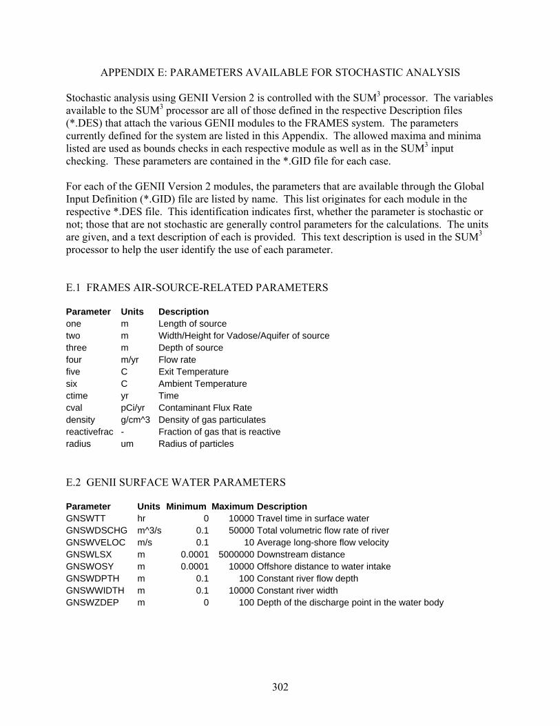
302

APPENDIX E: PARAMETERS AVAILABLE FOR STOCHASTIC ANALYSIS Stochastic analysis using GENII Version 2 is controlled with the SUM3 processor. The variables available to the SUM3 processor are all of those defined in the respective Description files (*.DES) that attach the various GENII modules to the FRAMES system. The parameters currently defined for the system are listed in this Appendix. The allowed maxima and minima listed are used as bounds checks in each respective module as well as in the SUM3 input checking. These parameters are contained in the *.GID file for each case. For each of the GENII Version 2 modules, the parameters that are available through the Global Input Definition (*.GID) file are listed by name. This list originates for each module in the respective *.DES file. This identification indicates first, whether the parameter is stochastic or not; those that are not stochastic are generally control parameters for the calculations. The units are given, and a text description of each is provided. This text description is used in the SUM3 processor to help the user identify the use of each parameter. E.1 FRAMES AIR-SOURCE-RELATED PARAMETERS Parameter Units Description one m Length of source two m Width/Height for Vadose/Aquifer of source three m Depth of source four m/yr Flow rate five C Exit Temperature six C Ambient Temperature ctime yr Time cval pCi/yr Contaminant Flux Rate density g/cm^3 Density of gas particulates reactivefrac - Fraction of gas that is reactive radius um Radius of particles

E.2 GENII SURFACE WATER PARAMETERS Parameter Units Minimum Maximum Description GNSWTT hr 0 10000 Travel time in surface water GNSWDSCHG m^3/s 0.1 50000 Total volumetric flow rate of river GNSWVELOC m/s 0.1 10 Average long-shore flow velocity GNSWLSX m 0.0001 5000000 Downstream distance GNSWOSY m 0.0001 10000 Offshore distance to water intake GNSWDPTH m 0.1 100 Constant river flow depth GNSWWIDTH m 0.1 10000 Constant river width GNSWZDEP m 0 100 Depth of the discharge point in the water body

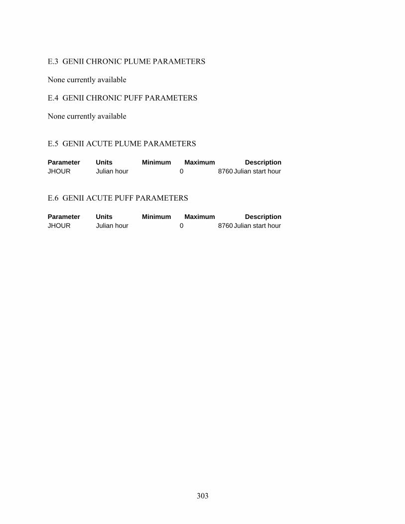
303

E.3 GENII CHRONIC PLUME PARAMETERS None currently available E.4 GENII CHRONIC PUFF PARAMETERS None currently available E.5 GENII ACUTE PLUME PARAMETERS Parameter Units Minimum Maximum Description JHOUR Julian hour 0 8760 Julian start hour E.6 GENII ACUTE PUFF PARAMETERS Parameter Units Minimum Maximum Description JHOUR Julian hour 0 8760 Julian start hour

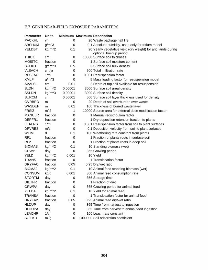
304

E.7 GENII NEAR-FIELD EXPOSURE PARAMETERS Parameter Units Minimum Maximum Description PACKHL yr 0 20 Waste package half life ABSHUM g/m^3 0 0.1 Absolute humidity, used only for tritium model YELDBT kg/m^2 0.1 20 Yearly vegetative yield (dry weight) for arid lands during

optional buildup period THICK cm 0 10000 Surface soil thickness MOISTC fraction 0 1 Surface soil moisture content BULKD g/cm^3 0.5 3 Surface soil bulk density VLEACH cm/yr 0 500 Total infiltration rate RESFAC 1/m 0 0.001 Resuspension factor XMLF g/m^3 0 5 Mass loading factor for resuspension model AVALSL cm 0.01 2 Depth of top soil available for resuspension SLDN kg/m^2 0.00001 3000 Surface soil areal density SSLDN kg/m^3 0.00001 3000 Surface soil density SURCM cm 0.00001 500 Surface soil layer thickness used for density OVRBRD m 0 20 Depth of soil overburden over waste WASDEP m 0.01 100 Thickness of buried waste layer FRSIZ m^2 1 10000 Source area for external dose modification factor MANULR fraction 0 1 Manual redistribution factor DEPFR1 fraction 0 1 Dry deposition retention fraction to plants LEAFRS 1/m 0 0.001 Resuspension factor from soil to plant surfaces DPVRES m/s 0 0.1 Deposition velocity from soil to plant surfaces WTIM d 0.1 100 Weathering rate constant from plants RF1 fraction 0 1 Fraction of plants roots in surface soil RF2 fraction 0 1 Fraction of plants roots in deep soil BIOMAS kg/m^2 0.1 10 Standing biomass (wet) GRWP day 0 365 Growing period YELD kg/m^2 0.001 10 Yield TRANS fraction 0 1 Translocation factor DRYFAC fraction 0.05 0.95 Dry/wet ratio BIOMA2 kg/m^2 0.1 10 Animal feed standing biomass (wet) CONSUM kg/d 0.001 300 Animal feed consumption rate STORTM day 0 356 Storage time DIETFR fraction 0 1 Fraction of diet GRWPA day 0 365 Growing period for animal feed YELDA kg/m^2 0.1 10 Yield for animal feed TRANSA fraction 0 1 Translocation factor for animal feed DRYFA2 fraction 0.05 0.95 Animal feed dry/wet ratio HLDUP day 0 365 Time from harvest to ingestion HLDUPA day 0 365 Time from harvest to animal feed ingestion LEACHR 1/yr 0 100 Leach rate constant SOILKD ml/g 0 1000000 Soil adsorbtion coefficient

305

E.8 GENII CHRONIC EXPOSURE PARAMETERS Parameter Units Minimum Maximum Description ABSHUM kg/m^3 0 0.1 Absolute humidity, used only for tritium model RF1 fraction 0 1 Fraction of plants roots in surface soil XMLF g/m^3 0 5 Mass loading factor for resuspension model AVALSL cm 0.01 200 Depth of top soil available for resuspension YELDA kg/m^2 0.1 10 Yield for animal feed HLDUPA day 0 365 Time from harvest to animal ingestion GRWPA day 0 365 Animal feed growing period STORTM day 0 356 Storage time DIETFR fraction 0 1 Fraction of diet YELD kg/m^2 0.001 10 Yield HLDUP day 0 365 Time from harvest to ingestion GRWP day 0 365 Growing period RIRRA in/yr 0 200 Animal feed irrigation rate IRTIMA mon/yr 0 12 Animal feed irrigation time RIRR in/yr 0 200 Irrigation rate IRTIMT mon/yr 0 12 Irrigation time HLDUP2 day 0 365 Time from harvest to ingestion DWFACA fraction 0 1 Animal water contaminated fraction SSLDN kg/m^3 0.00001 3000 Surface soil density RIRRR in/yr 0 200 Irrigation rate for residential land IRTIMR mon/yr 0 12 Irrigation time for residential land HOLDDW day 0 365 Delay time in water distribution system RESFAC 1/m 0 0.001 Resuspension factor WTIM d 0.1 100 Weathering rate constant from plants DEPFR1 fraction 0 1 Dry deposition retention fraction to plants RAIN mm/d 0.01 10 Average daily rain rate ANDKR l/m^3 0 10 Indoor volatilization factor for radionuclides SEDDN kg/m^2 0 5000 Shoreline sediment density THICK cm 0 10000 Surface soil thickness MOISTC fraction 0 1 Surface soil moisture content BULKD g/cm^3 0.5 3 Surface soil bulk density VLEACH cm/yr 0 500 Total infiltration rate DEPFR2 fraction 0 1 Wet deposition retention fraction to plant surfaces LEAFRS 1/m 0 0.001 Resuspension factor from soil to plant surfaces DPVRES m/s 0 0.1 Deposition velocity from soil to plant surfaces SLDN kg/m^2 0.00001 3000 Surface soil areal density SURCM cm 0.00001 500 Surface soil layer thickness used for density DWATER L/d 0.001 200 Intake rate of water BIOMA2 kg/m^2 0.1 10 Standing animal feed biomass (wet) CONSUM kg/d 0.001 300 Consumption rate BIOMAS kg/m^2 0.1 10 Standing biomass (wet) TRANSA fraction 0 1 Translocation factor for animal feed TRANS fraction 0 1 Translocation factor SLCONA kg/d 0 5 Animal daily soil consumption rate DRYFA2 fraction 0.05 0.95 Animal feed dry/wet ratio

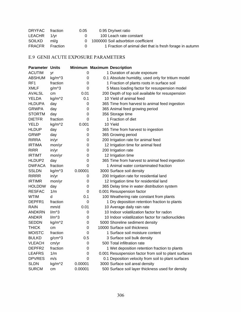
306

DRYFAC fraction 0.05 0.95 Dry/wet ratio LEACHR 1/yr 0 100 Leach rate constant SOILKD ml/g 0 1000000 Soil adsorbtion coefficient FRACFR Fraction 0 1 Fraction of animal diet that is fresh forage in autumn

E.9 GENII ACUTE EXPOSURE PARAMETERS Parameter Units Minimum Maximum Description ACUTIM yr 0 1 Duration of acute exposure ABSHUM kg/m^3 0 0.1 Absolute humidity, used only for tritium model RF1 fraction 0 1 Fraction of plants roots in surface soil XMLF g/m^3 0 5 Mass loading factor for resuspension model AVALSL cm 0.01 200 Depth of top soil available for resuspension YELDA kg/m^2 0.1 10 Yield of animal feed HLDUPA day 0 365 Time from harvest to animal feed ingestion GRWPA day 0 365 Animal feed growing period STORTM day 0 356 Storage time DIETFR fraction 0 1 Fraction of diet YELD kg/m^2 0.001 10 Yield HLDUP day 0 365 Time from harvest to ingestion GRWP day 0 365 Growing period RIRRA in/yr 0 200 Irrigation rate for animal feed IRTIMA mon/yr 0 12 Irrigation time for animal feed RIRR in/yr 0 200 Irrigation rate IRTIMT mon/yr 0 12 Irrigation time HLDUP2 day 0 365 Time from harvest to animal feed ingestion DWFACA fraction 0 1 Animal water contaminated fraction SSLDN kg/m^3 0.00001 3000 Surface soil density RIRRR in/yr 0 200 Irrigation rate for residential land IRTIMR mon/yr 0 12 Irrigation time for residential land HOLDDW day 0 365 Delay time in water distribution system RESFAC 1/m 0 0.001 Resuspension factor WTIM d 0.1 100 Weathering rate constant from plants DEPFR1 fraction 0 1 Dry deposition retention fraction to plants RAIN mm/d 0.01 10 Average daily rain rate ANDKRN l/m^3 0 10 Indoor volatilization factor for radon ANDKR l/m^3 0 10 Indoor volatilization factor for radionuclides SEDDN kg/m^2 0 5000 Shoreline sediment density THICK cm 0 10000 Surface soil thickness MOISTC fraction 0 1 Surface soil moisture content BULKD g/cm^3 0.5 3 Surface soil bulk density VLEACH cm/yr 0 500 Total infiltration rate DEPFR2 fraction 0 1 Wet deposition retention fraction to plants LEAFRS 1/m 0 0.001 Resuspension factor from soil to plant surfaces DPVRES m/s 0 0.1 Deposition velocity from soil to plant surfaces SLDN kg/m^2 0.00001 3000 Surface soil areal density SURCM cm 0.00001 500 Surface soil layer thickness used for density

307

DWATER L/d 0.001 200 Intake rate of water BIOMA2 kg/m^2 0.1 10 Standing biomass for animal feed (wet) CONSUM kg/d 0.001 300 Consumption rate BIOMAS kg/m^2 0.1 10 Standing biomass (wet) TRANSA fraction 0 1 Translocation factor for animal feed TRANS fraction 0 1 Translocation factor SLCONA kg/d 0 5 Animal daily soil consumption rate DRYFA2 fraction 0.05 0.95 Animal feed dry/wet ratio DRYFAC fraction 0.05 0.95 Dry/wet ratio FRACUT fraction 0 1 Fraction of diet that is fresh forage PROBAIR percent 0 100 Probability level for air concentration PROBDEP percent 0 100 Probability level for deposition rate PROBEXT percent 0 100 Probability level for external dose LEACHR 1/yr 0 100 Leach rate constant SOILKD ml/g 0 1000000 Soil adsorbtion coefficient FRACFR Fraction 0 1 Fraction of animal diet that is fresh forage in autumn

308

E.10 GENII RECEPTOR PARAMETERS Parameter Units Minimum Maximum Description UEXAIR hr 0 24 Daily plume immersion exposure time TEXAIR day 0 365 Yearly plume immersion exposure time SHIN none 0 1 Indoor shielding factor SHOUT none 0 1 Outdoor shielding factor UEXGRD hr 0 24 Daily external ground exposure time TEXGRD day 0 365 Yearly external ground exposure time FTIN fraction 0 1 Fraction of time spent indoors FTOUT fraction 0 1 Fraction of time spent outdoors EVSWIM evt/day 0 10 Frequency of swimming event TESWIM hr 0 24 Duration of swimming event TSWIM day 0 365 Swimming days USWIM L/hr 0 10 Ingestion rate of water while swimming SFBOAT none 0 1 Shielding factor EVBOAT evt/day 0 10 Frequency of boating event TEBOAT hr 0 24 Duration of boating event TBOAT day 0 365 Boating days EVSHOR evt/day 0 10 Frequency of shoreline use TESHOR hr 0 24 Duration of shoreline use events TSHOR day 0 365 Shoreline days SWFAC none 0 1 Shoreline width factor UCRP kg/day 0 10 Crop consumption rate TCRP day/yr 0 365 Crop consumption period UANM kg/day 0 10 Animal product consumption rate TANM day/yr 0 365 Animal product consumption period UAQU kg/day 0 10 Aquatic food consumption rate TAQU day/yr 0 365 Fish consumption period UDW L/day 0 10 Drinking water ingestion rate TDW day/yr 0 365 Drinking water ingestion period EVSHWR evt/day 0 10 Freqency of showering event TESHWR hr 0 24 Duration of showering event TSHWR day 0 365 Showering days USHIN L/hr 0 10 Ingestion rate of water while showering TSOIL day 0 365 Soil contact days USOIL mg/day 0 15000 Inadvertent soil ingestion rate UINH m^3/day 0 50 Air inhalation rate TINH day/yr 0 365 Air inhalation period UINHR m^3/day 0 50 Resuspended soil inhalation rate TINHR day/yr 0 365 Resuspended soil inhalation period FRINHR fraction 0 1 Fraction of a day inhalation occurs UINDRH m^3/day 0 50 Indoor air inhalation rate TINDRH day/yr 0 365 Indoor air inhalation period FRINDR fraction 0 1 Fraction of a day indoor inhalation occurs EQFRAC fraction 0 1 Radon progeny indoor equilibrium fraction

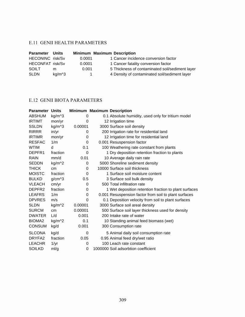
309

E.11 GENII HEALTH PARAMETERS Parameter Units Minimum Maximum Description HECONINC risk/Sv 0.0001 1 Cancer incidence conversion factor HECONFAT risk/Sv 0.0001 1 Cancer fatality conversion factor SOILT m 0.001 5 Thickness of contaminated soil/sediment layer SLDN kg/m^3 1 4 Density of contaminated soil/sediment layer

E.12 GENII BIOTA PARAMETERS Parameter Units Minimum Maximum Description ABSHUM kg/m^3 0 0.1 Absolute humidity, used only for tritium model IRTIMT mon/yr 0 12 Irrigation time SSLDN kg/m^3 0.00001 3000 Surface soil density RIRRR in/yr 0 200 Irrigation rate for residential land IRTIMR mon/yr 0 12 Irrigation time for residential land RESFAC 1/m 0 0.001 Resuspension factor WTIM d 0.1 100 Weathering rate constant from plants DEPFR1 fraction 0 1 Dry deposition retention fraction to plants RAIN mm/d 0.01 10 Average daily rain rate SEDDN kg/m^2 0 5000 Shoreline sediment density THICK cm 0 10000 Surface soil thickness MOISTC fraction 0 1 Surface soil moisture content BULKD g/cm^3 0.5 3 Surface soil bulk density VLEACH cm/yr 0 500 Total infiltration rate DEPFR2 fraction 0 1 Wet deposition retention fraction to plant surfaces LEAFRS 1/m 0 0.001 Resuspension factor from soil to plant surfaces DPVRES m/s 0 0.1 Deposition velocity from soil to plant surfaces SLDN kg/m^2 0.00001 3000 Surface soil areal density SURCM cm 0.00001 500 Surface soil layer thickness used for density DWATER L/d 0.001 200 Intake rate of water BIOMA2 kg/m^2 0.1 10 Standing animal feed biomass (wet) CONSUM kg/d 0.001 300 Consumption rate

SLCONA kg/d 0 5 Animal daily soil consumption rate DRYFA2 fraction 0.05 0.95 Animal feed dry/wet ratio LEACHR 1/yr 0 100 Leach rate constant SOILKD ml/g 0 1000000 Soil adsorbtion coefficient

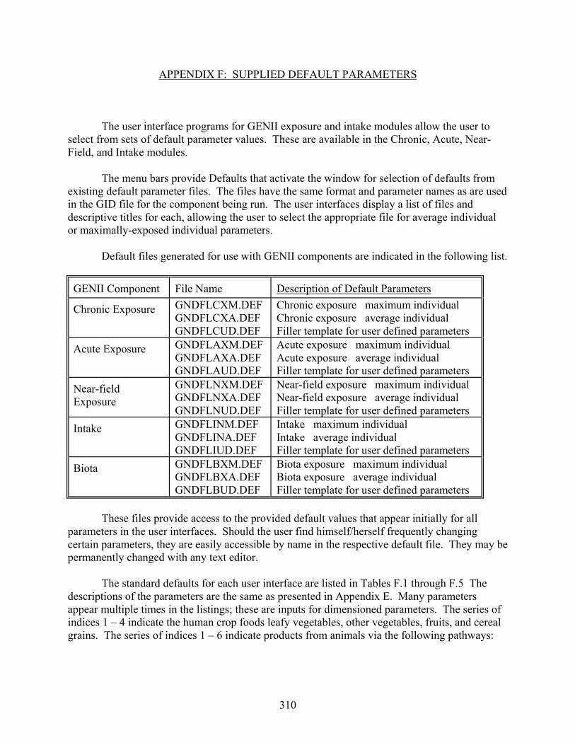
310

APPENDIX F: SUPPLIED DEFAULT PARAMETERS The user interface programs for GENII exposure and intake modules allow the user to select from sets of default parameter values. These are available in the Chronic, Acute, Near-Field, and Intake modules. The menu bars provide Defaults that activate the window for selection of defaults from existing default parameter files. The files have the same format and parameter names as are used in the GID file for the component being run. The user interfaces display a list of files and descriptive titles for each, allowing the user to select the appropriate file for average individual or maximally-exposed individual parameters. Default files generated for use with GENII components are indicated in the following list.

GENII Component File Name Description of Default Parameters

Chronic Exposure GNDFLCXM.DEF GNDFLCXA.DEF GNDFLCUD.DEF

Chronic exposure maximum individual Chronic exposure average individual Filler template for user defined parameters

Acute Exposure GNDFLAXM.DEF GNDFLAXA.DEF GNDFLAUD.DEF

Acute exposure maximum individual Acute exposure average individual Filler template for user defined parameters

Near-field Exposure

GNDFLNXM.DEF GNDFLNXA.DEF GNDFLNUD.DEF

Near-field exposure maximum individual Near-field exposure average individual Filler template for user defined parameters

Intake GNDFLINM.DEF GNDFLINA.DEF GNDFLIUD.DEF

Intake maximum individual Intake average individual Filler template for user defined parameters

Biota GNDFLBXM.DEF GNDFLBXA.DEF GNDFLBUD.DEF

Biota exposure maximum individual Biota exposure average individual Filler template for user defined parameters

These files provide access to the provided default values that appear initially for all

parameters in the user interfaces. Should the user find himself/herself frequently changing certain parameters, they are easily accessible by name in the respective default file. They may be permanently changed with any text editor.

The standard defaults for each user interface are listed in Tables F.1 through F.5 The descriptions of the parameters are the same as presented in Appendix E. Many parameters appear multiple times in the listings; these are inputs for dimensioned parameters. The series of indices 1 – 4 indicate the human crop foods leafy vegetables, other vegetables, fruits, and cereal grains. The series of indices 1 – 6 indicate products from animals via the following pathways:

311

meat cow feed, poultry feed, milk cow feed, egg hen feed, meat cow forage, and milk cow forage. Note that for the GENII Intake Module, up to six age groups may be defined. Currently, the adult defaults are used for all age groups because it is not known a priori how the age structure will be established by the user. As a result, if the defaults are selected, all age groups are initially assigned the adult parameters.

312

Table F.1 Defaults for GENII Acute Exposure Average and Maximum Individuals Parameter Index Units Average Maximum

IRES 0 N/A 0 0 IRRSA 1 N/A 0 0 IRRSA 2 N/A 0 0 IRRSA 3 N/A 0 0 IRRSA 4 N/A 0 0 IRRSA 5 N/A 0 0 IRRSA 6 N/A 0 0 IRRST 1 N/A 0 0 IRRST 2 N/A 0 0 IRRST 3 N/A 0 0 IRRST 4 N/A 0 0 IRRSR 0 N/A 0 0

LEACHOPTION

0 N/A 1 1

DWSRC 0 N/A 0 0 INHAL 0 N/A FALSE FALSE

ANFOOD 0 N/A TRUE TRUE TFOOD 0 N/A TRUE TRUE

AQFOOD 0 N/A TRUE TRUE RECRE 0 N/A TRUE TRUE DEBUG 0 N/A FALSE FALSE

DWTRET 0 N/A TRUE TRUE RESIRR 0 N/A TRUE TRUE FINITE 0 N/A FALSE FALSE AIREXT 0 N/A FALSE FALSE

ANF 1 N/A FALSE FALSE ANF 2 N/A FALSE FALSE ANF 3 N/A FALSE FALSE ANF 4 N/A FALSE FALSE TFD 1 N/A FALSE FALSE TFD 2 N/A FALSE FALSE TFD 3 N/A FALSE FALSE TFD 4 N/A FALSE FALSE AQF 1 N/A FALSE FALSE AQF 2 N/A FALSE FALSE AQF 3 N/A FALSE FALSE AQF 4 N/A FALSE FALSE

DRINK 0 N/A FALSE FALSE SHING 0 N/A FALSE FALSE SWING 0 N/A FALSE FALSE SLING 0 N/A FALSE FALSE

SHINDR 0 N/A FALSE FALSE SLINH 0 N/A FALSE FALSE REC 1 N/A FALSE FALSE

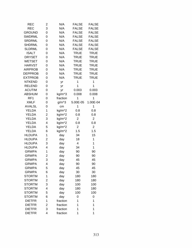
313

REC 2 N/A FALSE FALSE REC 3 N/A FALSE FALSE

GROUND 0 N/A FALSE FALSE SWDRML 0 N/A FALSE FALSE SRDRML 0 N/A FALSE FALSE SHDRML 0 N/A FALSE FALSE SLDRML 0 N/A FALSE FALSE

ISALT 0 N/A TRUE TRUE DRYSET 0 N/A TRUE TRUE WETSET 0 N/A TRUE TRUE HARVST 0 N/A TRUE TRUE AIRPROB 0 N/A TRUE TRUE DEPPROB 0 N/A TRUE TRUE EXTPROB 0 N/A TRUE TRUE NTKEND 0 yr 1 1 RELEND 0 yr 1 1 ACUTIM 0 yr 0.003 0.003 ABSHUM 0 kg/m^3 0.008 0.008

RF1 0 fraction 1 1 XMLF 0 g/m^3 5.00E-05 1.00E-04

AVALSL 0 cm 1 1 YELDA 1 kg/m^2 0.8 0.8 YELDA 2 kg/m^2 0.8 0.8 YELDA 3 kg/m^2 2 2 YELDA 4 kg/m^2 0.8 0.8 YELDA 5 kg/m^2 2 2 YELDA 6 kg/m^2 1.5 1.5

HLDUPA 1 day 34 15 HLDUPA 2 day 18 1 HLDUPA 3 day 4 1 HLDUPA 4 day 34 1 GRWPA 1 day 90 90 GRWPA 2 day 90 90 GRWPA 3 day 45 45 GRWPA 4 day 90 90 GRWPA 5 day 45 45 GRWPA 6 day 30 30 STORTM 1 day 180 180 STORTM 2 day 180 180 STORTM 3 day 100 100 STORTM 4 day 180 180 STORTM 5 day 100 100 STORTM 6 day 0 0 DIETFR 1 fraction 1 1 DIETFR 2 fraction 1 1 DIETFR 3 fraction 1 1 DIETFR 4 fraction 1 1

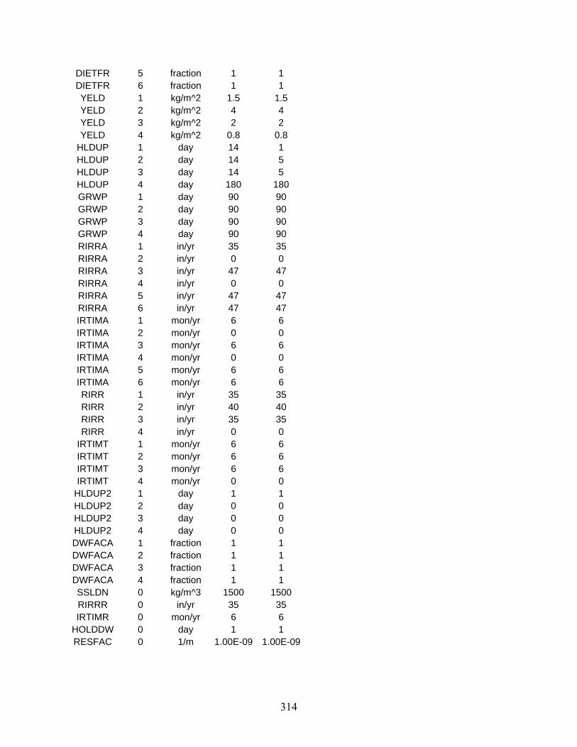
314

DIETFR 5 fraction 1 1 DIETFR 6 fraction 1 1 YELD 1 kg/m^2 1.5 1.5 YELD 2 kg/m^2 4 4 YELD 3 kg/m^2 2 2 YELD 4 kg/m^2 0.8 0.8

HLDUP 1 day 14 1 HLDUP 2 day 14 5 HLDUP 3 day 14 5 HLDUP 4 day 180 180 GRWP 1 day 90 90 GRWP 2 day 90 90 GRWP 3 day 90 90 GRWP 4 day 90 90 RIRRA 1 in/yr 35 35 RIRRA 2 in/yr 0 0 RIRRA 3 in/yr 47 47 RIRRA 4 in/yr 0 0 RIRRA 5 in/yr 47 47 RIRRA 6 in/yr 47 47 IRTIMA 1 mon/yr 6 6 IRTIMA 2 mon/yr 0 0 IRTIMA 3 mon/yr 6 6 IRTIMA 4 mon/yr 0 0 IRTIMA 5 mon/yr 6 6 IRTIMA 6 mon/yr 6 6 RIRR 1 in/yr 35 35 RIRR 2 in/yr 40 40 RIRR 3 in/yr 35 35 RIRR 4 in/yr 0 0

IRTIMT 1 mon/yr 6 6 IRTIMT 2 mon/yr 6 6 IRTIMT 3 mon/yr 6 6 IRTIMT 4 mon/yr 0 0

HLDUP2 1 day 1 1 HLDUP2 2 day 0 0 HLDUP2 3 day 0 0 HLDUP2 4 day 0 0 DWFACA 1 fraction 1 1 DWFACA 2 fraction 1 1 DWFACA 3 fraction 1 1 DWFACA 4 fraction 1 1 SSLDN 0 kg/m^3 1500 1500 RIRRR 0 in/yr 35 35 IRTIMR 0 mon/yr 6 6

HOLDDW 0 day 1 1 RESFAC 0 1/m 1.00E-09 1.00E-09

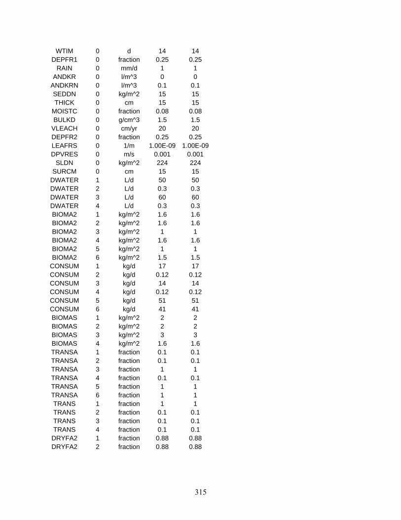
315

WTIM 0 d 14 14 DEPFR1 0 fraction 0.25 0.25

RAIN 0 mm/d 1 1 ANDKR 0 l/m^3 0 0

ANDKRN 0 l/m^3 0.1 0.1 SEDDN 0 kg/m^2 15 15 THICK 0 cm 15 15

MOISTC 0 fraction 0.08 0.08 BULKD 0 g/cm^3 1.5 1.5

VLEACH 0 cm/yr 20 20 DEPFR2 0 fraction 0.25 0.25 LEAFRS 0 1/m 1.00E-09 1.00E-09DPVRES 0 m/s 0.001 0.001

SLDN 0 kg/m^2 224 224 SURCM 0 cm 15 15

DWATER 1 L/d 50 50 DWATER 2 L/d 0.3 0.3 DWATER 3 L/d 60 60 DWATER 4 L/d 0.3 0.3 BIOMA2 1 kg/m^2 1.6 1.6 BIOMA2 2 kg/m^2 1.6 1.6 BIOMA2 3 kg/m^2 1 1 BIOMA2 4 kg/m^2 1.6 1.6 BIOMA2 5 kg/m^2 1 1 BIOMA2 6 kg/m^2 1.5 1.5

CONSUM 1 kg/d 17 17 CONSUM 2 kg/d 0.12 0.12 CONSUM 3 kg/d 14 14 CONSUM 4 kg/d 0.12 0.12 CONSUM 5 kg/d 51 51 CONSUM 6 kg/d 41 41 BIOMAS 1 kg/m^2 2 2 BIOMAS 2 kg/m^2 2 2 BIOMAS 3 kg/m^2 3 3 BIOMAS 4 kg/m^2 1.6 1.6 TRANSA 1 fraction 0.1 0.1 TRANSA 2 fraction 0.1 0.1 TRANSA 3 fraction 1 1 TRANSA 4 fraction 0.1 0.1 TRANSA 5 fraction 1 1 TRANSA 6 fraction 1 1 TRANS 1 fraction 1 1 TRANS 2 fraction 0.1 0.1 TRANS 3 fraction 0.1 0.1 TRANS 4 fraction 0.1 0.1

DRYFA2 1 fraction 0.88 0.88 DRYFA2 2 fraction 0.88 0.88

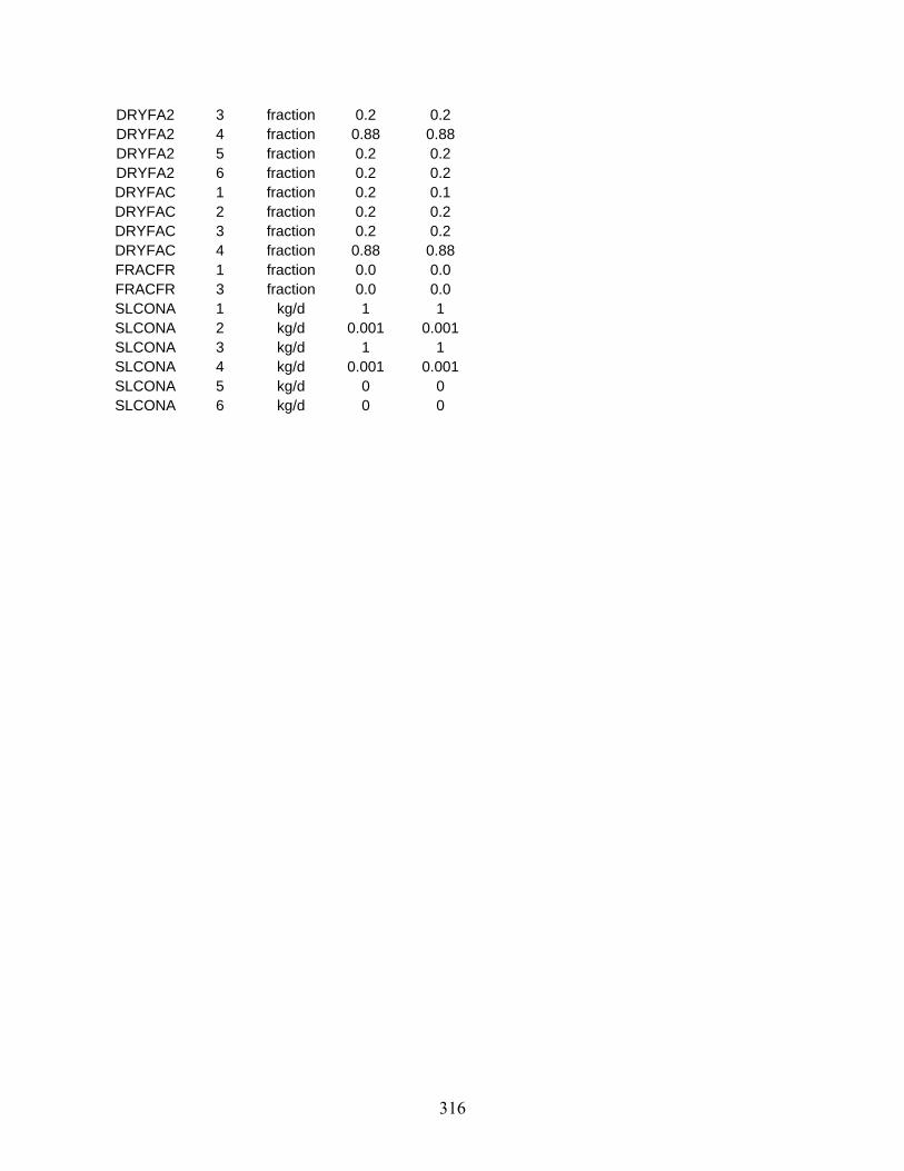
316

DRYFA2 3 fraction 0.2 0.2 DRYFA2 4 fraction 0.88 0.88 DRYFA2 5 fraction 0.2 0.2 DRYFA2 6 fraction 0.2 0.2 DRYFAC 1 fraction 0.2 0.1 DRYFAC 2 fraction 0.2 0.2 DRYFAC 3 fraction 0.2 0.2 DRYFAC 4 fraction 0.88 0.88 FRACFR 1 fraction 0.0 0.0 FRACFR 3 fraction 0.0 0.0 SLCONA 1 kg/d 1 1 SLCONA 2 kg/d 0.001 0.001 SLCONA 3 kg/d 1 1 SLCONA 4 kg/d 0.001 0.001 SLCONA 5 kg/d 0 0 SLCONA 6 kg/d 0 0

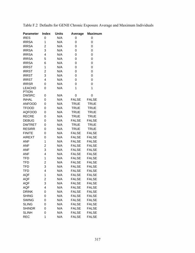
317

Table F.2 Defaults for GENII Chronic Exposure Average and Maximum Individuals Parameter Index Units Average MaximumIRES 0 N/A 0 0 IRRSA 1 N/A 0 0 IRRSA 2 N/A 0 0 IRRSA 3 N/A 0 0 IRRSA 4 N/A 0 0 IRRSA 5 N/A 0 0 IRRSA 6 N/A 0 0 IRRST 1 N/A 0 0 IRRST 2 N/A 0 0 IRRST 3 N/A 0 0 IRRST 4 N/A 0 0 IRRSR 0 N/A 0 0 LEACHOPTION

0 N/A 1 1

DWSRC 0 N/A 0 0 INHAL 0 N/A FALSE FALSE ANFOOD 0 N/A TRUE TRUE TFOOD 0 N/A TRUE TRUE AQFOOD 0 N/A TRUE TRUE RECRE 0 N/A TRUE TRUE DEBUG 0 N/A FALSE FALSE DWTRET 0 N/A TRUE TRUE RESIRR 0 N/A TRUE TRUE FINITE 0 N/A FALSE FALSE AIREXT 0 N/A FALSE FALSE ANF 1 N/A FALSE FALSE ANF 2 N/A FALSE FALSE ANF 3 N/A FALSE FALSE ANF 4 N/A FALSE FALSE TFD 1 N/A FALSE FALSE TFD 2 N/A FALSE FALSE TFD 3 N/A FALSE FALSE TFD 4 N/A FALSE FALSE AQF 1 N/A FALSE FALSE AQF 2 N/A FALSE FALSE AQF 3 N/A FALSE FALSE AQF 4 N/A FALSE FALSE DRINK 0 N/A FALSE FALSE SHING 0 N/A FALSE FALSE SWING 0 N/A FALSE FALSE SLING 0 N/A FALSE FALSE SHINDR 0 N/A FALSE FALSE SLINH 0 N/A FALSE FALSE REC 1 N/A FALSE FALSE

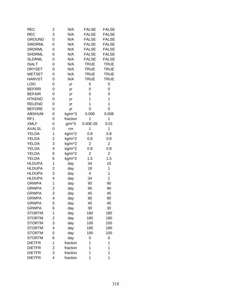
318

REC 2 N/A FALSE FALSE REC 3 N/A FALSE FALSE GROUND 0 N/A FALSE FALSE SWDRML 0 N/A FALSE FALSE SRDRML 0 N/A FALSE FALSE SHDRML 0 N/A FALSE FALSE SLDRML 0 N/A FALSE FALSE ISALT 0 N/A TRUE TRUE DRYSET 0 N/A TRUE TRUE WETSET 0 N/A TRUE TRUE HARVST 0 N/A TRUE TRUE LOIC 0 yr 0 0 BEFIRR 0 yr 0 0 BEFAIR 0 yr 0 0 NTKEND 0 yr 1 1 RELEND 0 yr 1 1 BEFORE 0 yr 0 0 ABSHUM 0 kg/m^3 0.008 0.008 RF1 0 fraction 1 1 XMLF 0 g/m^3 5.00E-05 0.01 AVALSL 0 cm 1 1 YELDA 1 kg/m^2 0.8 0.8 YELDA 2 kg/m^2 0.8 0.8 YELDA 3 kg/m^2 2 2 YELDA 4 kg/m^2 0.8 0.8 YELDA 5 kg/m^2 2 2 YELDA 6 kg/m^2 1.5 1.5 HLDUPA 1 day 34 15 HLDUPA 2 day 18 1 HLDUPA 3 day 4 1 HLDUPA 4 day 34 1 GRWPA 1 day 90 90 GRWPA 2 day 90 90 GRWPA 3 day 45 45 GRWPA 4 day 90 90 GRWPA 5 day 45 45 GRWPA 6 day 30 30 STORTM 1 day 180 180 STORTM 2 day 180 180 STORTM 3 day 100 100 STORTM 4 day 180 180 STORTM 5 day 100 100 STORTM 6 day 0 0 DIETFR 1 fraction 1 1 DIETFR 2 fraction 1 1 DIETFR 3 fraction 1 1 DIETFR 4 fraction 1 1

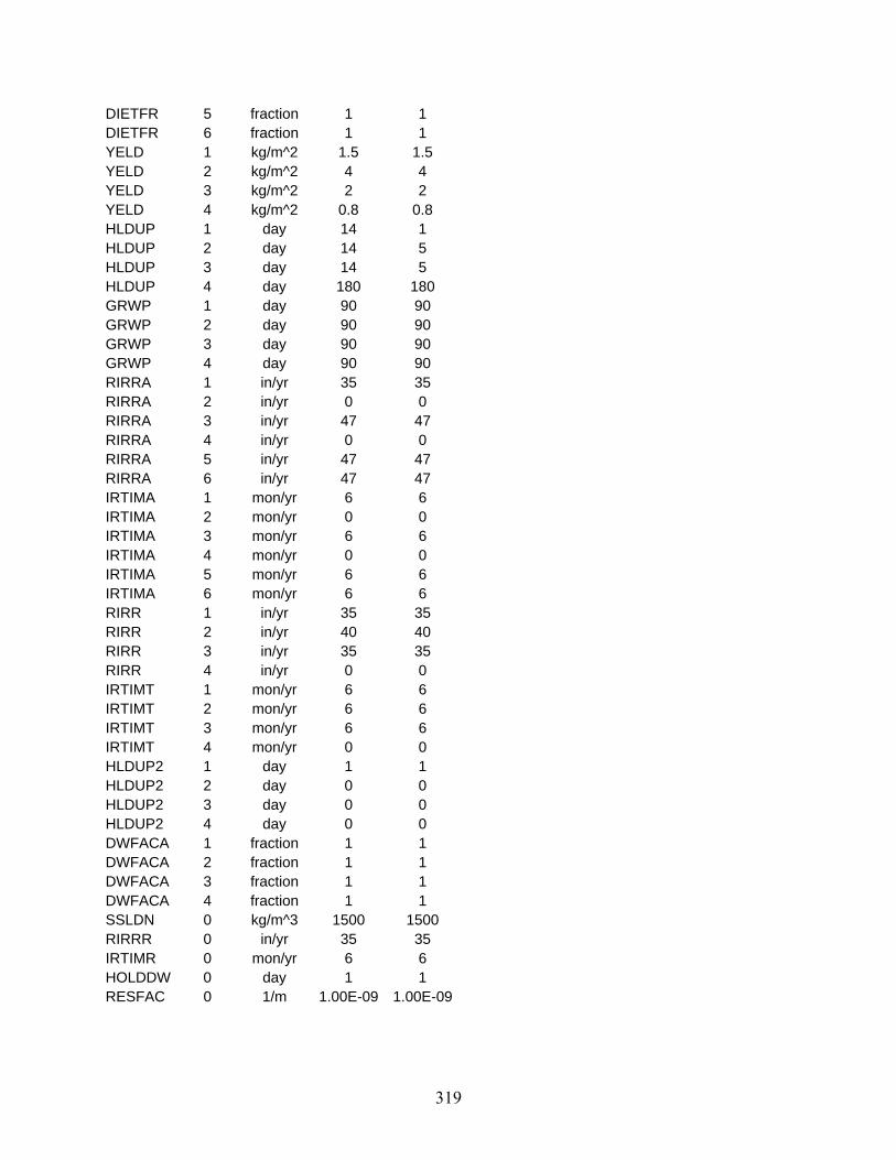
319

DIETFR 5 fraction 1 1 DIETFR 6 fraction 1 1 YELD 1 kg/m^2 1.5 1.5 YELD 2 kg/m^2 4 4 YELD 3 kg/m^2 2 2 YELD 4 kg/m^2 0.8 0.8 HLDUP 1 day 14 1 HLDUP 2 day 14 5 HLDUP 3 day 14 5 HLDUP 4 day 180 180 GRWP 1 day 90 90 GRWP 2 day 90 90 GRWP 3 day 90 90 GRWP 4 day 90 90 RIRRA 1 in/yr 35 35 RIRRA 2 in/yr 0 0 RIRRA 3 in/yr 47 47 RIRRA 4 in/yr 0 0 RIRRA 5 in/yr 47 47 RIRRA 6 in/yr 47 47 IRTIMA 1 mon/yr 6 6 IRTIMA 2 mon/yr 0 0 IRTIMA 3 mon/yr 6 6 IRTIMA 4 mon/yr 0 0 IRTIMA 5 mon/yr 6 6 IRTIMA 6 mon/yr 6 6 RIRR 1 in/yr 35 35 RIRR 2 in/yr 40 40 RIRR 3 in/yr 35 35 RIRR 4 in/yr 0 0 IRTIMT 1 mon/yr 6 6 IRTIMT 2 mon/yr 6 6 IRTIMT 3 mon/yr 6 6 IRTIMT 4 mon/yr 0 0 HLDUP2 1 day 1 1 HLDUP2 2 day 0 0 HLDUP2 3 day 0 0 HLDUP2 4 day 0 0 DWFACA 1 fraction 1 1 DWFACA 2 fraction 1 1 DWFACA 3 fraction 1 1 DWFACA 4 fraction 1 1 SSLDN 0 kg/m^3 1500 1500 RIRRR 0 in/yr 35 35 IRTIMR 0 mon/yr 6 6 HOLDDW 0 day 1 1 RESFAC 0 1/m 1.00E-09 1.00E-09

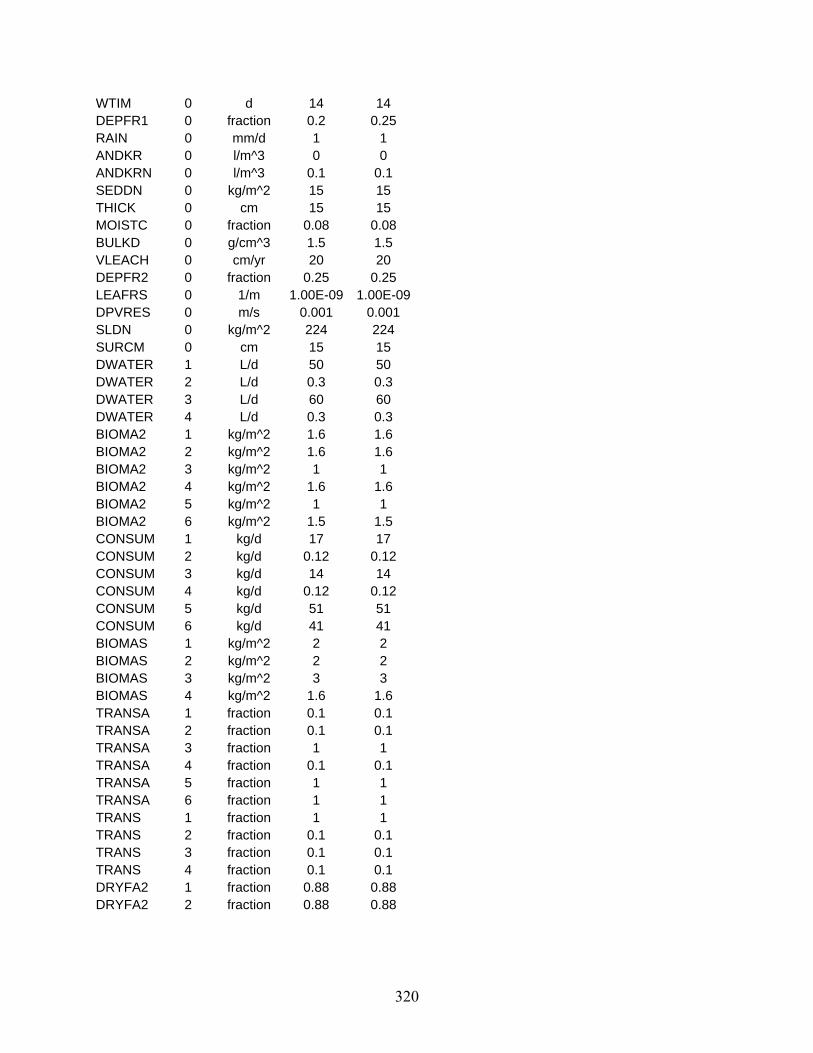
320

WTIM 0 d 14 14 DEPFR1 0 fraction 0.2 0.25 RAIN 0 mm/d 1 1 ANDKR 0 l/m^3 0 0 ANDKRN 0 l/m^3 0.1 0.1 SEDDN 0 kg/m^2 15 15 THICK 0 cm 15 15 MOISTC 0 fraction 0.08 0.08 BULKD 0 g/cm^3 1.5 1.5 VLEACH 0 cm/yr 20 20 DEPFR2 0 fraction 0.25 0.25 LEAFRS 0 1/m 1.00E-09 1.00E-09DPVRES 0 m/s 0.001 0.001 SLDN 0 kg/m^2 224 224 SURCM 0 cm 15 15 DWATER 1 L/d 50 50 DWATER 2 L/d 0.3 0.3 DWATER 3 L/d 60 60 DWATER 4 L/d 0.3 0.3 BIOMA2 1 kg/m^2 1.6 1.6 BIOMA2 2 kg/m^2 1.6 1.6 BIOMA2 3 kg/m^2 1 1 BIOMA2 4 kg/m^2 1.6 1.6 BIOMA2 5 kg/m^2 1 1 BIOMA2 6 kg/m^2 1.5 1.5 CONSUM 1 kg/d 17 17 CONSUM 2 kg/d 0.12 0.12 CONSUM 3 kg/d 14 14 CONSUM 4 kg/d 0.12 0.12 CONSUM 5 kg/d 51 51 CONSUM 6 kg/d 41 41 BIOMAS 1 kg/m^2 2 2 BIOMAS 2 kg/m^2 2 2 BIOMAS 3 kg/m^2 3 3 BIOMAS 4 kg/m^2 1.6 1.6 TRANSA 1 fraction 0.1 0.1 TRANSA 2 fraction 0.1 0.1 TRANSA 3 fraction 1 1 TRANSA 4 fraction 0.1 0.1 TRANSA 5 fraction 1 1 TRANSA 6 fraction 1 1 TRANS 1 fraction 1 1 TRANS 2 fraction 0.1 0.1 TRANS 3 fraction 0.1 0.1 TRANS 4 fraction 0.1 0.1 DRYFA2 1 fraction 0.88 0.88 DRYFA2 2 fraction 0.88 0.88

321

DRYFA2 3 fraction 0.2 0.2 DRYFA2 4 fraction 0.88 0.88 DRYFA2 5 fraction 0.2 0.2 DRYFA2 6 fraction 0.2 0.2 DRYFAC 1 fraction 0.1 0.1 DRYFAC 2 fraction 0.2 0.2 DRYFAC 3 fraction 0.2 0.2 DRYFAC 4 fraction 0.88 0.88 SLCONA 1 kg/d 1 1 SLCONA 2 kg/d 0.001 0.001 SLCONA 3 kg/d 1 1 SLCONA 4 kg/d 0.001 0.001 SLCONA 5 kg/d 0 0 SLCONA 6 kg/d 0 0

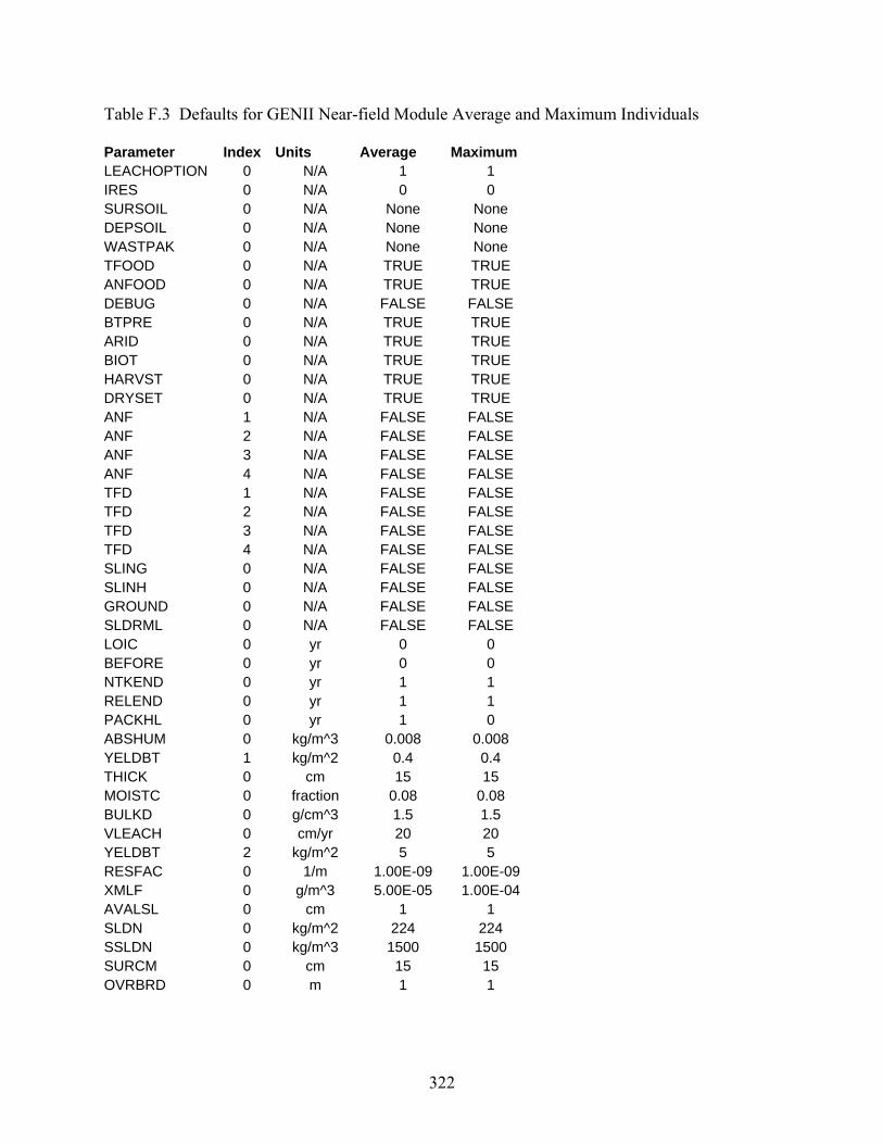
322

Table F.3 Defaults for GENII Near-field Module Average and Maximum Individuals Parameter Index Units Average Maximum LEACHOPTION 0 N/A 1 1 IRES 0 N/A 0 0 SURSOIL 0 N/A None None DEPSOIL 0 N/A None None WASTPAK 0 N/A None None TFOOD 0 N/A TRUE TRUE ANFOOD 0 N/A TRUE TRUE DEBUG 0 N/A FALSE FALSE BTPRE 0 N/A TRUE TRUE ARID 0 N/A TRUE TRUE BIOT 0 N/A TRUE TRUE HARVST 0 N/A TRUE TRUE DRYSET 0 N/A TRUE TRUE ANF 1 N/A FALSE FALSE ANF 2 N/A FALSE FALSE ANF 3 N/A FALSE FALSE ANF 4 N/A FALSE FALSE TFD 1 N/A FALSE FALSE TFD 2 N/A FALSE FALSE TFD 3 N/A FALSE FALSE TFD 4 N/A FALSE FALSE SLING 0 N/A FALSE FALSE SLINH 0 N/A FALSE FALSE GROUND 0 N/A FALSE FALSE SLDRML 0 N/A FALSE FALSE LOIC 0 yr 0 0 BEFORE 0 yr 0 0 NTKEND 0 yr 1 1 RELEND 0 yr 1 1 PACKHL 0 yr 1 0 ABSHUM 0 kg/m^3 0.008 0.008 YELDBT 1 kg/m^2 0.4 0.4 THICK 0 cm 15 15 MOISTC 0 fraction 0.08 0.08 BULKD 0 g/cm^3 1.5 1.5 VLEACH 0 cm/yr 20 20 YELDBT 2 kg/m^2 5 5 RESFAC 0 1/m 1.00E-09 1.00E-09 XMLF 0 g/m^3 5.00E-05 1.00E-04 AVALSL 0 cm 1 1 SLDN 0 kg/m^2 224 224 SSLDN 0 kg/m^3 1500 1500 SURCM 0 cm 15 15 OVRBRD 0 m 1 1

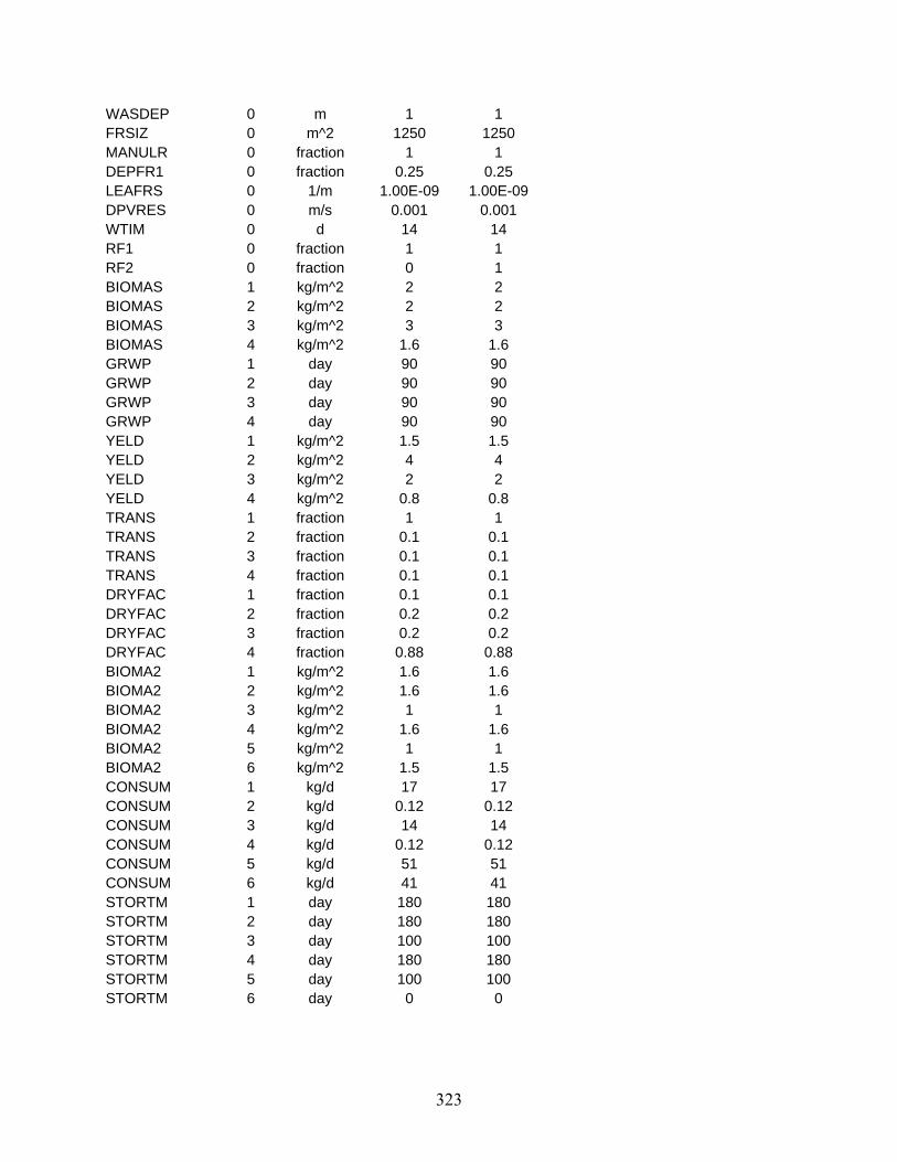
323

WASDEP 0 m 1 1 FRSIZ 0 m^2 1250 1250 MANULR 0 fraction 1 1 DEPFR1 0 fraction 0.25 0.25 LEAFRS 0 1/m 1.00E-09 1.00E-09 DPVRES 0 m/s 0.001 0.001 WTIM 0 d 14 14 RF1 0 fraction 1 1 RF2 0 fraction 0 1 BIOMAS 1 kg/m^2 2 2 BIOMAS 2 kg/m^2 2 2 BIOMAS 3 kg/m^2 3 3 BIOMAS 4 kg/m^2 1.6 1.6 GRWP 1 day 90 90 GRWP 2 day 90 90 GRWP 3 day 90 90 GRWP 4 day 90 90 YELD 1 kg/m^2 1.5 1.5 YELD 2 kg/m^2 4 4 YELD 3 kg/m^2 2 2 YELD 4 kg/m^2 0.8 0.8 TRANS 1 fraction 1 1 TRANS 2 fraction 0.1 0.1 TRANS 3 fraction 0.1 0.1 TRANS 4 fraction 0.1 0.1 DRYFAC 1 fraction 0.1 0.1 DRYFAC 2 fraction 0.2 0.2 DRYFAC 3 fraction 0.2 0.2 DRYFAC 4 fraction 0.88 0.88 BIOMA2 1 kg/m^2 1.6 1.6 BIOMA2 2 kg/m^2 1.6 1.6 BIOMA2 3 kg/m^2 1 1 BIOMA2 4 kg/m^2 1.6 1.6 BIOMA2 5 kg/m^2 1 1 BIOMA2 6 kg/m^2 1.5 1.5 CONSUM 1 kg/d 17 17 CONSUM 2 kg/d 0.12 0.12 CONSUM 3 kg/d 14 14 CONSUM 4 kg/d 0.12 0.12 CONSUM 5 kg/d 51 51 CONSUM 6 kg/d 41 41 STORTM 1 day 180 180 STORTM 2 day 180 180 STORTM 3 day 100 100 STORTM 4 day 180 180 STORTM 5 day 100 100 STORTM 6 day 0 0

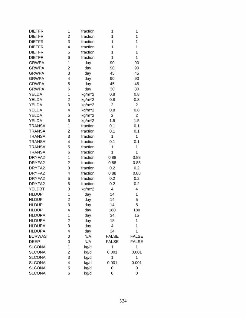
324

DIETFR 1 fraction 1 1 DIETFR 2 fraction 1 1 DIETFR 3 fraction 1 1 DIETFR 4 fraction 1 1 DIETFR 5 fraction 1 1 DIETFR 6 fraction 1 1 GRWPA 1 day 90 90 GRWPA 2 day 90 90 GRWPA 3 day 45 45 GRWPA 4 day 90 90 GRWPA 5 day 45 45 GRWPA 6 day 30 30 YELDA 1 kg/m^2 0.8 0.8 YELDA 2 kg/m^2 0.8 0.8 YELDA 3 kg/m^2 2 2 YELDA 4 kg/m^2 0.8 0.8 YELDA 5 kg/m^2 2 2 YELDA 6 kg/m^2 1.5 1.5 TRANSA 1 fraction 0.1 0.1 TRANSA 2 fraction 0.1 0.1 TRANSA 3 fraction 1 1 TRANSA 4 fraction 0.1 0.1 TRANSA 5 fraction 1 1 TRANSA 6 fraction 1 1 DRYFA2 1 fraction 0.88 0.88 DRYFA2 2 fraction 0.88 0.88 DRYFA2 3 fraction 0.2 0.2 DRYFA2 4 fraction 0.88 0.88 DRYFA2 5 fraction 0.2 0.2 DRYFA2 6 fraction 0.2 0.2 YELDBT 3 kg/m^2 4 4 HLDUP 1 day 14 1 HLDUP 2 day 14 5 HLDUP 3 day 14 5 HLDUP 4 day 180 180 HLDUPA 1 day 34 15 HLDUPA 2 day 18 1 HLDUPA 3 day 4 1 HLDUPA 4 day 34 1 BURWAS 0 N/A FALSE FALSE DEEP 0 N/A FALSE FALSE SLCONA 1 kg/d 1 1 SLCONA 2 kg/d 0.001 0.001 SLCONA 3 kg/d 1 1 SLCONA 4 kg/d 0.001 0.001 SLCONA 5 kg/d 0 0 SLCONA 6 kg/d 0 0

325

Table F.4 Defaults for GENII Intake Module Average and Maximum Individuals Parameter Index Units Average MaximumNAGES 0 N/A 1 1 EDAGE 0 yr 70 70 POPAGE 0 none 1 1 UEXAIR 0 hr 24 24 TEXAIR 0 day 365 365 SHIN 0 none 1 1 SHOUT 0 none 1 1 UEXGRD 0 hr 24 24 TEXGRD 0 day 121.7 182.5 FTIN 0 fraction 0.7 0.7 FTOUT 0 fraction 0.3 0.3 EVSWIM 0 evt/day 1 1 TESWIM 0 hr 2 2 TSWIM 0 day 5 50 SFBOAT 0 none 1 1 EVBOAT 0 evt/day 1 1 TEBOAT 0 hr 1 2 TBOAT 0 day 5 50 EVSHOR 0 evt/day 1 1 TESHOR 0 hr 3.3 5 TSHOR 0 day 5 100 SWFAC 0 none 0.2 0.2 UCRP 1 kg/day 0.041 0.082 TCRP 1 day/yr 365 365 UCRP 2 kg/day 0.383 0.602 TCRP 2 day/yr 365 365 UCRP 3 kg/day 0.175 0.903 TCRP 3 day/yr 365 365 UCRP 4 kg/day 0.197 0.219 TCRP 4 day/yr 365 365 UANM 1 kg/day 0.192 0.219 TANM 1 day/yr 365 365 UANM 2 kg/day 0.023 0.049 TANM 2 day/yr 365 365 UANM 3 kg/day 0.63 0.739 TANM 3 day/yr 365 365 UANM 4 kg/day 0.055 0.082 TANM 4 day/yr 365 365 UAQU 1 kg/day 0.019 0.11 TAQU 1 day/yr 365 365 UAQU 2 kg/day 0 0.019 TAQU 2 day/yr 365 365 UAQU 3 kg/day 0 0.019 TAQU 3 day/yr 365 365

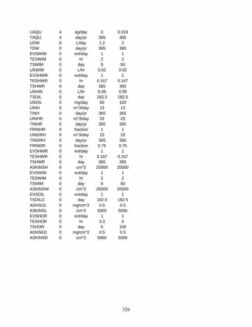
326

UAQU 4 kg/day 0 0.019 TAQU 4 day/yr 365 365 UDW 0 L/day 1.2 2 TDW 0 day/yr 365 365 EVSWIM 0 evt/day 1 1 TESWIM 0 hr 2 2 TSWIM 0 day 5 50 USWIM 0 L/hr 0.02 0.02 EVSHWR 0 evt/day 1 1 TESHWR 0 hr 0.167 0.167 TSHWR 0 day 365 365 USHIN 0 L/hr 0.06 0.06 TSOIL 0 day 182.5 182.5 USOIL 0 mg/day 50 100 UINH 0 m^3/day 13 13 TINH 0 day/yr 365 365 UINHR 0 m^3/day 23 23 TINHR 0 day/yr 365 365 FRINHR 0 fraction 1 1 UINDRH 0 m^3/day 10 10 TINDRH 0 day/yr 365 365 FRINDR 0 fraction 0.75 0.75 EVSHWR 0 evt/day 1 1 TESHWR 0 hr 0.167 0.167 TSHWR 0 day 365 365 ASKINSH 0 cm^2 20000 20000 EVSWIM 0 evt/day 1 1 TESWIM 0 hr 2 2 TSWIM 0 day 5 50 ASKINSW 0 cm^2 20000 20000 EVSOIL 0 evt/day 1 1 TSOILD 0 day 182.5 182.5 ADHSOL 0 mg/cm^2 0.5 0.5 ASKINSL 0 cm^2 5000 5000 EVSHOR 0 evt/day 1 1 TESHOR 0 hr 3.3 5 TSHOR 0 day 5 100 ADHSED 0 mg/cm^2 0.5 0.5 ASKINSD 0 cm^2 5000 5000

327

Table F.5 Defaults for GENII Biota Module Average and Maximum Exposures

Parameter Index Units Average Maximum

BEFIRR 0 yr 0 0

BEFAIR 0 yr 0 0

NTKEND 0 yr 1 1

RELEND 0 yr 1 1

BEFORE 0 yr 0 0

ABSHUM 0 kg/m^3 0.008 0.008

SSLDN 0 kg/m^3 1500 1500

RIRRR 0 in/yr 35 35

IRTIMR 0 mon/yr 6 6

RESFAC 0 1/m 1.00E-09 1.00E-09

WTIM 0 d 14 14

DEPFR1 0 fraction 0.25 0.25

RAIN 0 mm/d 1 1

SEDDN 0 kg/m^2 15 15

THICK 0 cm 15 15

MOISTC 0 fraction 0.08 0.08

BULKD 0 g/cm^3 1.5 1.5

VLEACH 0 cm/yr 20 20

DEPFR2 0 fraction 0.25 0.25

LEAFRS 0 1/m 1.00E-09 1.00E-09

DPVRES 0 m/s 0.001 0.001

SLDN 0 kg/m^2 224 224

SURCM 0 cm 15 15

DWATER 1 L/d 30 30

DWATER 2 L/d 0.3 0.3

DWATER 3 L/d 30 30

DWATER 4 L/d 0.3 0.3

DWATER 5 L/d 0.3 0.3

BIOMA2 1 kg/m^2 1.5 1.5

BIOMA2 2 kg/m^2 1.5 1.5

BIOMA2 3 kg/m^2 1.5 1.5

BIOMA2 4 kg/m^2 1.5 1.5

BIOMA2 5 kg/m^2 1.5 1.5

BIOMA2 6 kg/m^2 1.5 1.5

CONSUM 1 kg/d 5 5

CONSUM 2 kg/d 0.12 0.12

CONSUM 3 kg/d 2 2

328

CONSUM 4 kg/d 0.12 0.12

CONSUM 5 kg/d 0.12 0.12

DRYFA2 1 fraction 0.2 0.2

DRYFA2 2 fraction 0.2 0.2

DRYFA2 3 fraction 0.2 0.2

DRYFA2 4 fraction 0.2 0.2

DRYFA2 5 fraction 0.2 0.2

DRYFA2 6 fraction 0.2 0.2

SLCONA 1 kg/d 1 1

SLCONA 2 kg/d 0.001 0.001

SLCONA 3 kg/d 1 1

SLCONA 4 kg/d 0.001 0.001

SLCONA 5 kg/d 0.001 0.001

RATIME 1 hr/yr 2922 2922

RATIME 2 hr/yr 2922 2922

RATIME 3 hr/yr 8760 8760

RATIME 4 hr/yr 8760 8760